modern map methods in particle beam...
TRANSCRIPT

Modern Map Methods in Particle Beam Physics
MARTIN BERZ
Department of Physics Michigan State University East Lansing, Michigan

This book provides a general introduction to the single particle dynamics of beams. It is based on lectures given at Michigan State University, including the Virtual University Program in Beam Physics, as well as the US Particle Accelerator School and the CERN Academic Training Programme. It is rounded out by providing as much as possible of the necessary physics and mathematics background, and as such is rather self-contained. In an educational curriculum for beam physics, it represents an intermediate level following an introduction of general concepts of beam physics, although much of it can also be mastered independently of such previous knowledge. Its level of treatment should be suitable for graduate students, and much of it can also be mastered by upper division undergraduate students.
The expose is based on map theory for the description of the motion, and extensive use is made of the framework of the differential algebraic approach developed by the author, which is the only method that allows computations of nonlinearities of the maps to arbitrary order. Furthermore, it lends itself to a particularly transparent presentation and analysis of all relevant nonlinear effects. The tools and algorithms presented here are available directly in the code COSY INFINITY. Many tools from the theory of dynamical systems and electrodynamics are included; in particular, we provide a modern and rigorous account of Hamiltonian theory.
Copyright © 1999 by Martin Berz
ACADEMIC PRESS A Harcourt Science and Technology Company 24-28 Oval Road, London NW1 7DX, UK http://www.academicpress.com
International Standard Book Number 0-12-014750-5
CONTENTS
CHAPTER 1 Dynamics of Particles and Fields
1.1 Beams and Beam Physics ......................................................................................... 1 1.2 Differential Equations, Determinism, and Maps ....................................................... 2 1.2.1 Existence and Uniqueness of Solutions ....................................................... 3 1.2.2 Maps of Deterministic Differential Equations ............................................. 6 1.3 Lagrangian Systems ................................................................................................... 7 1.3.1 Existence and Uniqueness of Lagrangians .................................................. 7 1.3.2 Canonical Transformation of Lagrangians .................................................. 8 1.3.3 Connection to a Variational Principle ....................................................... 12 1.3.4 Lagrangians for Particular Systems ........................................................... 14 1.4 Hamiltonian Systems .............................................................................................. 20 1.4.1 Manipulations of the Independent Variable .............................................. 23 1.4.2 Existence and Uniqueness of Hamiltonians .............................................. 26 1.4.3 The Duality of Hamiltonians and Lagrangians .......................................... 27 1.4.4 Hamiltonians for Particular Systems ......................................................... 32 1.4.5 Canonical Transformation of Hamiltonians .............................................. 34 1.4.6 Universal Existence of Generating Functions ........................................... 44 1.4.7 Flows of Hamiltonian Systems ................................................................. 53 1.4.8 Generating Functions ................................................................................ 54 1.4.9 Time-Dependent Canonical Transformations ........................................... 59 1.4.10 The Hamilton-Jacobi Equation .................................................................. 60 1.5 Fields and Potentials ............................................................................................... 62 1.5.1 Maxwell's Equations ................................................................................. 62 1.5.2 Scalar and Vector Potentials ...................................................................... 65 1.5.3 Boundary Value Problems ......................................................................... 76

CHAPTER 2 Differential Algebraic Techniques
2.1 Function Spaces and Their Algebras ....................................................................... 82 2.1.1 Floating Point Numbers and Intervals ....................................................... 82 2.1.2 Representations of Functions .................................................................... 82 2.1.3 Algebras and Differential Algebras ........................................................... 84 2.2 Taylor Differential Algebras .................................................................................... 86 2.2.1 The Minimal Differential Algebra ............................................................. 86 2.2.2 The Differential Algebra nDv ..................................................................... 91 2.2.3 Generators, Bases, and Order .................................................................... 92 2.2.4 The Tower of Ideals, Nilpotency, and Fixed Points .................................. 96 2.3 Advanced Methods ................................................................................................. 100 2.3.1 Composition and Inversion ..................................................................... 100 2.3.2 Important Elementary Functions ............................................................. 102 2.3.3 Power Series on nDv ................................................................................ 104 2.3.4 ODE and PDE Solvers ............................................................................ 108 2.3.5 The Levi-Civita Field .............................................................................. 111
CHAPTER 3 Fields
3.1 Analytic Field Representation ............................................................................... 120 3.1.1 Fields with Straight Reference Orbit ....................................................... 120 3.1.2 Fields with Planar Reference Orbit ......................................................... 125 3.2 Practical Utilization of Field Information ............................................................. 126 3.2.1 Multipole Measurements ......................................................................... 127 3.2.2 Midplane Field Measurements ................................................................ 128 3.2.3 Electric Image Charge Methods .............................................................. 129 3.2.4 Magnetic Image Charge Methods ........................................................... 132 3.2.5 The Method of Wire Currents ................................................................. 139

CHAPTER 4 Maps: Properties
4.1 Manipulations ....................................................................................................... 146 4.1.1 Composition and Inversion ..................................................................... 146 4.1.2 Reversion ................................................................................................. 147 4.2 Symmetries ........................................................................................................... 148 4.2.1 Midplane Symmetry ................................................................................ 148 4.2.2 Rotational Symmetry ............................................................................... 150 4.2.3 Symplectic Symmetry ............................................................................. 155 4.3 Representations ..................................................................................................... 159 4.3.1 Flow Factorizations ................................................................................. 159 4.3.2 Generating Functions .............................................................................. 164
CHAPTER 5 Maps: Calculation
5.1 The Particle Optical Equations of Motion ............................................................ 168 5.1.1 Curvilinear Coordinates .......................................................................... 169 5.1.2 The Lagrangian and Lagrange's Equations in Curvilinear Coordinates ... 175 5.1.3 The Hamiltonian and Hamilton's Equations in Curvilinear Coordinates . 179 5.1.4 Arc Length as an Independent Variable for the Hamiltonian .................. 185 5.1.5 Curvilinear Coordinates for Planar Motion ............................................. 188 5.2 Equations of Motion for Spin ................................................................................ 190 5.3 Maps Determined by Algebraic Relations ............................................................ 195 5.3.1 Lens Optics ............................................................................................... 195 5.3.2 The Dipole ................................................................................................ 197 5.3.3 Drifts and Kicks ....................................................................................... 201 5.4 Maps Determined by Differential Equations ........................................................ 201 5.4.1 Differentiating ODE Solvers ................................................................... 201 5.4.2 DA Solvers for Differential Equations ..................................................... 202 5.4.3 Fast Perturbative Approximations ............................................................ 203

CHAPTER 6 Imaging Systems
6.1 Introduction ........................................................................................................... 211 6.2 Aberrations and their Correction ........................................................................... 214 6.3 Reconstructive Correction of Aberrations ............................................................ 217 6.3.1 Trajectory Reconstruction ....................................................................... 218 6.3.2 Reconstruction in Energy Loss Mode ..................................................... 221 6.3.3 Examples and Applications ..................................................................... 223 6.4 Aberration Correction via Repetitive Symmetry .................................................. 228 6.4.1 Second-Order Achromats . ...................................................................... 230 6.4.2 Map Representations ............................................................................... 233 6.4.3 Major Correction Theorems .................................................................... 238 6.4.4 A Snake-Shaped Third-Order Achromat ................................................. 240 6.4.5 Repetitive Third-and Fifth Order Achromats .......................................... 243
CHAPTER 7 Repetitive Systems
7.1 Linear Theory ........................................................................................................ 250 7.1.1 The Stability of the Linear Motion. ......................................................... 250 7.1.2 The Invariant Ellipse of Stable Symplectic Motion ................................ 260 7.1.3 Transformations of Elliptical Phase Space. ............................................. 262 7.2 Parameter Dependent Linear Theory .................................................................... 265 7.2.1 The Closed Orbit ..................................................................................... 266 7.2.2 Parameter Tune Shifts ............................................................................. 267 7.2.3 Chromaticity Correction .......................................................................... 268 7.3 Normal Forms ....................................................................................................... 270 7.3.1 The DA Normal Form Algorithm ............................................................ 270 7.3.2 Symplectic Systems ................................................................................. 274 7.3.3 Non-Symplectic Systems ........................................................................ 277 7.3.4 Amplitude Tune Shifts and Resonances .................................................. 279 7.3.5 Invariants and Stability Estimates ........................................................... 282 7.3.6 Spin Normal Forms ................................................................................. 288 7.4 Symplectic Tracking ............................................................................................. 292 7.4.1 Generating Functions .............................................................................. 293 7.4.2 Pre-Factorization and Symplectic Extension ........................................... 295 7.4.3 Superposition of Local Generators .......................................................... 297 7.4.4 Factorizations in Integrable Symplectic Maps ......................................... 298 7.4.5 Spin Tracking .......................................................................................... 299

ACKNOWLEDGMENTS
I am grateful to a number of individuals who have contributed in various ways to this text. Foremost I would like to thank the many students who participated in the various versions of these lectures and provided many useful suggestions. My thanks go to Kyoko Makino and Weishi Wan, who even actively contributed certain parts of this book. Specifically, I thank Kyoko for the derivation and documentation of the Hamiltonian in curvilinear coordinates (Section 5.1) and Weishi for being the main impetus in the development and documentation of the theory of nonlinear correction (Section 6.4). In the earlier stages of the preparation of the manuscript, we enjoyed various discussions with Georg Hoffstätter. To Khodr Shamseddine I am grateful for skillfully preparing many of the figures. For a careful reading of parts the manuscript, I would like to thank Kyoko Makino, Khodr Shamseddine, Bela Erdelyi, and Jens von Bergmann. I am also thankful to Peter Hawkes, the editor of the series in which this book is appearing, for his ongoing encouragement and support, as well as the staff at Academic Press for the skilled and professional preparation of the final layout. Last but not least, I am grateful for financial support through grants from the U.S. Department of Energy and a fellowship from the Alfred P. Sloan foundation. Martin Berz Summer 1999
Errata corrected until January 2013

Chapter 1
Dynamics of Particles and Fields
1.1 BEAMS AND BEAM PHYSICS
In a very general sense, the field of beam physics is concerned with the analysisof the dynamics of certain state vectors ��� These comprise the coordinates ofinterest, and their motion is described by a differential equation ���� �� � ������ ���Usually it is necessary to analyze the manifold of solutions of the differentialequation not only for one state vector �� but also for an entire ensemble of statevectors. Different from other disciplines, in the field of beam physics the ensembleof state vectors is usually somewhat close together and also stays that way overthe range of the dynamics. Such an ensemble of nearby state vectors is calleda beam.
The study of the dynamics of beams has two important subcategories: the de-scription of the motion to very high precision over short times and the analysis ofthe topology of the evolution of state space over long times. These subcategoriescorrespond to the historical foundations of beam physics, which lie in the twoseemingly disconnected fields of optics and celestial mechanics. In the case ofoptics, in order to make an image of an object or to spectroscopically analyze thedistributions of colors, it is important to guide the individual rays in a light beamto very clearly specified final conditions. In the case of celestial mechanics, theprecise calculation of orbits over short terms is also of importance, for example,for the prediction of eclipses or the assessment of orbits of newly discovered as-teroids under consideration of the uncertainties of initial conditions. Furthermore,celestial mechanics is also concerned with the question of stability of a set ofpossible initial states over long periods of time, one of the first and fundamentalconcerns of the field of nonlinear dynamics; it may not be relevant where ex-actly the earth is located in a billion years as long as it is still approximately thesame distance away from the sun. Currently, we recognize these fields as just twospecific cases of the study of weakly nonlinear motion which are linked by thecommon concept of the so-called transfer map of the dynamics.
On the practical side, currently the study of beams is important because beamscan provide and carry two fundamentally important scientific concepts, namely,energy and information. Energy has to be provided through acceleration, and thesignificance of this aspect is reflected in the name accelerator physics, which is of-ten used almost synonymously with beam physics. Information is either generated
1 Copyright c� 1999 by Martin BerzAll rights of reproduction in any form reserved.

2 DYNAMICS OF PARTICLES AND FIELDS
by utilizing the beam’s energy, in which case it is analyzed through spectroscopy,or it is transported at high rates and is thus relevant for the practical aspects ofinformation science.
Applications of these two concepts are wide. The field of high-energy physicsor particle physics utilizes both aspects of beams, and these aspects are so im-portant that they are directly reflected in their names. First, common particles arebrought to energies far higher than those found anywhere else on earth. Then thisenergy is utilized in collisions to produce particles that do not exist in our currentnatural environment, and information about such new particles is extracted.
In a similar way, nuclear physics uses the energy of beams to produce isotopesthat do not exist in our natural environment and extracts information about theirproperties. It also uses beams to study the dynamics of the interaction of nuclei.Both particle physics and nuclear physics also re-create the state of our universewhen it was much hotter, and beams are used to artificially generate the ambienttemperature at these earlier times. Currently, two important questions relate to theunderstanding of the time periods close to the big bang as well as the understand-ing of nucleosynthesis, the generation of the currently existing different chemicalelements.
In chemistry and material science, beams provide tools to study the detailsof the dynamics of chemical reactions and a variety of other questions. In manycases, these studies are performed using intense light beams, which are producedin conventional lasers, free-electron lasers, or synchrotron light sources.
Also, great progress continues to be made in the traditional roots of the field ofbeam physics, optics, and celestial mechanics. Modern glass lenses for camerasare better, more versatile, and used now more than ever before, and modern elec-tron microscopes now achieve unprecedented resolutions in the Angstrom range.Celestial mechanics has made considerable progress in the understanding of thenonlinear dynamics of planets and the prospects for the long-term stability of oursolar system; for example, while the orbit of earth does not seem to be in jeop-ardy at least for the medium term, there are other dynamical quantities of the solarsystem that behave chaotically.
Currently, the ability to transport information is being applied in the case offiber optics, in which short light pulses provide very high transfer rates. Also,electron beams transport the information in the television tube, belonging to oneof the most widespread consumer products that, for better or worse, has a signifi-cant impact on the values of our modern society.
1.2 DIFFERENTIAL EQUATIONS, DETERMINISM, AND MAPS
As discussed in the previous section, the study of beams is connected to the un-derstanding of solutions of differential equations for an ensemble of related ini-tial conditions. In the following sections, we provide the necessary framework tostudy this question.

DIFFERENTIAL EQUATIONS, DETERMINISM, AND MAPS 3
1.2.1 Existence and Uniqueness of Solutions
Let us consider the differential equation
�
���� � �� ���� ��� (1.1)
where �� is a state vector that satisfies the initial condition ������ � ���� In practicethe vector �� can comprise positions, momenta or velocities, or any other quantityinfluencing the motion, such as a particle’s spin, mass, or charge. We note that theordinary differential equation (ODE) being of first order is immaterial becauseany higher order differential equation
��
����� � ��
����
�
����� � � � �
����
�������
�(1.2)
can be rewritten as a first-order differential equation; by introducing the � � ��new variables ��� � ������� ��� � ��������� � � � � ����� � ������������, we havethe equivalent first-order system
�
��
�����
�����...
�����
����� �
�����
������...
������ ���� � � � � ������
����� � (1.3)
Furthermore, it is possible to rewrite the differential equation in terms of anyother independent variable that satisfies
�
���� � (1.4)
and hence depends strictly monotonically on �� Indeed, in this case we have
�
��� �
�
���� � ��
�� ������ ���� � ��
�� (1.5)
Similarly, the question of dependence on the independent variable is immaterialbecause an explicitly �-dependent differential equation can be rewritten as a �-independent differential equation by the introduction of an additional variable with ���� � � and substitution of � by in the equation:
�
��
���
��
������� ��
�� (1.6)
Frequently, one studies the evolution of a particular quantity that depends onthe phase space variables along a solution of the ODE. For a given differentiable
4 DYNAMICS OF PARTICLES AND FIELDS
function � ���� �� from phase space into the real numbers (such a function is alsooften called an observable), it is possible to determine its derivative and hence anassociated ODE describing its motion via
�
��� ���� �� � �� � ��� �
�
��� � �� ���� (1.7)
the differential operator �� is usually called the vector field of the ODE. Othercommon names are directional derivative or Lie derivative. It plays an impor-tant role in the theory of dynamical systems and will be used repeatedly in theremainder of the text. Apparently, the differential operator can also be used todetermine higher derivatives of � by repeated application of �� , and we have
��
���� � �
���� (1.8)
An important question in the study of differential equations is whether anysolutions exist and, if so, whether they are unique. The first part of the question isanswered by the theorem of Peano; as long as the function �� is continuous in aneighborhood of ����� ���, the existence of a solution is guaranteed at least in aneighborhood.
The second question is more subtle than one might think at first glance. Forexample, it is ingrained in our thinking that classical mechanics is deterministic,which means that the value of a state at a given time �� uniquely specifies the valueof the state at any later time �� However, this is not always the case; consider theHamiltonian and its equations of motion:
� ���
�� � ���� where � ��� � ������� (1.9)
� � � and � � sign���
�������� (1.10)
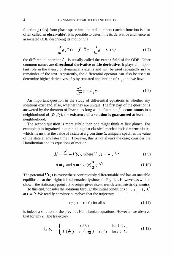
The potential � ��� is everywhere continuously differentiable and has an unstableequilibrium at the origin; it is schematically shown in Fig. 1.1. However, as will beshown, the stationary point at the origin gives rise to nondeterministic dynamics.
To this end, consider the solutions through the initial condition �� �� ��� � ��� ��at � � �� We readily convince ourselves that the trajectory
��� �� � ��� �� for all � (1.11)
is indeed a solution of the previous Hamiltonian equations. However, we observethat for any ��, the trajectory
��� �� �
��� �� for � � ��
� ��� ��� ���
�� ��� ��� ���
��
for � � ��(1.12)

DIFFERENTIAL EQUATIONS, DETERMINISM, AND MAPS 5
FIGURE 1.1. A nondeterministic potential.
is a solution of the differential equations! This means that the particle has a choiceof staying on top of the equilibrium point or, at any time � � it pleases, it can startto leave the equilibrium point, either toward the left or toward the right. Certainly,there is no determinism anymore.
In a deeper sense, the problem is actually more far-reaching than one may think.While the previous example may appear somewhat pathological, one can showthat any potential � ��� can be modified by adding a second term �� ��� with� ��� continuous and �� ���� � � such that for any �, the potential � ������ ���is nondeterministic. Choosing � smaller than the accuracy to which potentials canbe measured, we conclude that determinism in classical mechanics is principallyundecidable.
In a mathematical sense, the second question is answered by the Picard-Lindelof Theorem, which asserts that if the right-hand side �� of the differentialequation (1.1) satisfies a Lipschitz condition with respect to ��, i.e., there is a �such that
�������� ��� ������� ��� � � � ���� � ���� (1.13)
for all ���, ��� and for all �, then there is a unique solution in a neighborhood ofany ����� ����
Therefore, determinism of classical mechanics can be assured if one axiomat-ically assumes the Lipschitzness of the forces that can appear in classical me-chanics. This axiom of determinism of mechanics, however, is more delicate thanother axioms in physics because it cannot be checked experimentally in a directway, as the previous example of the potential � shows.

6 DYNAMICS OF PARTICLES AND FIELDS
1.2.2 Maps of Deterministic Differential Equations
Let us assume we are given a deterministic system
�
���� � ������ ��� (1.14)
which means that for every initial condition ��� at ��� there is a unique solution����� with ������ � ���� For a given time ��, this allows to introduce a func-tion ������ that for any initial condition ��� determines the value of the solutionthrough ����� ��� at the later time ��� therefore we have
������ ������������� (1.15)
The function� describes how individual state space points “flow” as time pro-gresses, and in the theory of dynamical systems it is usually referred to as the flowof the differential equation. We also refer to it as the propagator (describing howstate space points are propagated), the transfer map (describing how state spacepoints are transferred), or simply the map. It is obvious that the transfer mapssatisfy the property
������ ������� ������ (1.16)
where “Æ” stands for the composition of functions. In particular, we have
� ������� ������ � (1.17)
and so the transfer maps are invertible.An important case is the situation in which the ODE is autonomous, i.e.,
� independent. In this case, the transfer map depends only on the difference�� � �� � ��, and we have
�������� ����� ���� � (1.18)
An important case of dynamical systems is the situation in which the motion isrepetitive, which means that there is a �� such that
������� ������������� (1.19)
In this case, the long-term behavior of the motion can be analyzed by merelystudying the repeated action of �������. If the motion suits our needs for thediscrete time steps �� and occupies a suitable set � of state spaces there, then itis merely necessary to study once how this set � is transformed for intermediatetimes between � and ���� and whether this satisfies our needs. This stroboscopicstudy of repetitive motion is an important example of the method of Poincare

LAGRANGIAN SYSTEMS 7
sections, of which there are several varieties including suitable changes of theindependent variables but these always amount to the study of repetitive motionby discretization.
In the following sections, we embark on the study of one of the most impor-tant classes of dynamical systems, namely, those that can be expressed within theframeworks of the theories of Lagrange, Hamilton, and Jacobi.
1.3 LAGRANGIAN SYSTEMS
Let us assume we are given a dynamical system of quantities ��� � � � � �� whosedynamics is described by a second-order differential equation of the form
��
�� � �� ��� ����
���� (1.20)
If there exists a function depending on �� and�
��, i.e.,
� �����
��� ��� (1.21)
such that the equations
�
��
��
� �
�� �
��� �� � � �� � � � � (1.22)
are equivalent to the equations of motion (1.20) of the system, then is calleda Lagrangian for this system. In this case, equations (1.22) are known as La-grange’s equations of motion. There are usually many advantages if equations ofmotion can be rewritten in terms of a Lagrangian; the one that is perhaps moststraightforwardly appreciated is that the motion is now described by a singlescalar function instead of the components of �� � However, there are otheradvantages because Lagrangian systems have special properties, many of whichare discussed in the following sections.
1.3.1 Existence and Uniqueness of Lagrangians
Before we proceed, we may ask ourselves whether a function �����
��� �� always ex-ists and, if so, whether it is unique. The latter part of the question apparently has
to be negated because Lagrangians are not unique. Apparently with �����
��� ��
also �����
��� ��� �, where � is a constant, is also a Lagrangian for �� � Furthermore,a constant � can be added not only to , but also more generally to any func-
tion ������
��� �� that satisfies ����(�����
���� ������ � � for all choices of �� and�
�� � Such functions do indeed exist; for example, the function ������
��� �� � �� ��
��

8 DYNAMICS OF PARTICLES AND FIELDS
apparently satisfies the requirement. Trying to generalize this example, one real-
izes that while the linearity with respect to�
�� is important, the dependence on ��can be more general; also, a dependence on time is possible, if it is connectedin the proper way to the position dependence. Altogether, if � is a three timesdifferentiable function depending on position �� and �, then
������
��� �� ��
��� ���� �� �
���
��
��� � � ��
��(1.23)
satisfies ����������
���� ������ � �; indeed, studying the �th component of thecondition yields
�
��
�
� �
�� ��
�
��
��� � � ��
��
��� �
��
�� ��
�
��
��� � � ��
��
��
��
��
���
��
��
���
���
����� � � ���
����
�
���
���
����� � � ���
�����
���
���
����� � � ���
����� �� (1.24)
The question of existence cannot be answered in a general way, but fortu-nately for many systems of practical relevance to us, Lagrangians can be found.This usually requires some “guessing” for every special case of interest; manyexamples for this can be found in Section 1.3.4.
One of the important advantages of the Lagrangian formulation is that it isparticularly easy to perform transformations to different sets of variables, as illus-trated in the next section.
1.3.2 Canonical Transformation of Lagrangians
Given a system described by coordinates ���� � � � � ���, its analysis can often besimplified by studying it in a set of different coordinates. One important case ismotion that is subject to certain constraints; in this case, one can often performa change of coordinates in such a way that a given constraint condition merelymeans that one of the new coordinates is to be kept constant. For example, if aparticle is constrained to move along a circular loop, then expressing its motion inpolar coordinates ��� �� concentric with the loop instead of in Cartesian variablesallows the simplification of the constraint condition to the simple statement that� is kept constant. This reduces the dimensionality of the problem and leads toa new system free of constraints, and thus this approach is frequently appliedfor the study of constrained systems. Currently, there is also an important field

LAGRANGIAN SYSTEMS 9
that studies such constrained systems or differential algebraic equations directlywithout removal of the constraints (Ascher and Petzold 1998; Griepentrog andMarz 1986; Brenan, Campbell, and Petzold 1989; Matsuda 1980).
Another important case is the situation in which certain invariants of the mo-tion are known to exist; if these invariants can be introduced as new variables,it again follows that these variables are constant, and the dimensionality of thesystem can be reduced. More sophisticated changes of coordinates relevant to ourgoals will be discussed later.
It is worth noting that the choice of new variables does not have to be thesame everywhere in variable space but may change from one region to another;this situation can be dealt with in a natural and organized way with the theory ofmanifolds in which the entire region of interest is covered by an atlas, which isa collection of local coordinate systems called charts that are patched together tocover the entire region of interest and to overlap smoothly. However, we do notneed to discuss these issues in detail.
Let a Lagrangian system with coordinates ���� � � � � ��� be given. Let���� � � � � ��� be another set of coordinates, and let be the transformationfrom the old to the new coordinates, which is allowed to be time dependent, suchthat
�� � ���� ��� (1.25)
The transformation is demanded to be invertible, and hence we have
�� � ��� ��� ��� (1.26)
furthermore, let both of the transformations be continuously differentiable. Alto-gether, the change of variables constitutes an isomorphism that is continuouslydifferentiable in both directions, a so-called diffeomorphism.
In the following, we will often not distinguish between the symbol describingthe transformation function and the symbol describing the new coordinates ��if it is clear from the context which one is meant. The previous transformationequations then appear as
�� � ������ �� and �� � ��� ��� ��� (1.27)
where �� and �� on the left side of the equations and inside the parentheses denote-tuples, while in front of the parentheses they denote functions. While this latterconvention admittedly has the danger of appearing logically paradoxical if notunderstood properly, it often simplifies the nomenclature to be discussed later.
If the coordinates transform according to Eq. (1.25), then the corresponding
time derivatives�
�� transform according to
�
�� � Jac(����� �� ��
�� ����
� (1.28)

10 DYNAMICS OF PARTICLES AND FIELDS
and we obtain the entire transformation� from (����
��� to � ����
��� as ���
��
��
� ���� ��Jac(����� �� �
�
�� � ����
�������
�
��� ��� (1.29)
It is a remarkable and most useful fact that in order to find a Lagrangian that
describes the motion in the new variables �� and�
�� from the Lagrangian describing
the motion in the variables �� and�
��, it is necessary only to insert the transformation
rule (Eq. 1.26) as well as the resulting time derivative�
�� ��
��� ����
��� �� into the
Lagrangian, and thus it depends on �� and�
�� � We say that the Lagrangian isinvariant under a coordinate transformation. Therefore, the new Lagrangianwill be given by
�� ����
��� �� � ��� ��� ���
�
�� � ����
��� ��� ��� (1.30)
or in terms of the transformation maps,
� � ����� and � ����� (1.31)
In order to prove this property, let us assume that � �����
��� �� is a Lagrangiandescribing the motion in the coordinates ��, i.e.,
�
��
��
� �
�� �
��� �� � � �� � � � � (1.32)
yield the proper equations of motion of the system.Differentiating Eqs. (1.25) and (1.26) with respect to time, as is necessary for
the substitution into the Lagrangian, we obtain
�
�� ��
�������
��� ��
�
�� ��
��� ����
��� ��� (1.33)
We now perform the substitution of Eqs. (1.26) and (1.33) into (1.30) and let
�� ����
��� �� be the resulting function; that is,
�� ����
��� �� � ��� ��� ���
�
�� � ����
��� ��� ��� (1.34)
The goal is now to show that indeed
�
��
���
� �
�� ��
��� �� � � �� � � � � � (1.35)

LAGRANGIAN SYSTEMS 11
We fix a � � . Then
��
� �
���
�
�
� �
� �
� �
(1.36)
and
��
���
���
�
��
����
���
�
�
� �
� ���
� (1.37)
Thus,
�
��
��
� �
��
��
��
�
�
� �
� �
� �
�
���
�
��
��
�
� �
�� �
� �
���
�
�
� �
�
��
� �
� �
��
Note that from
� ���
��
�����
�� �����
� (1.38)
we obtain � ��� � � ����� . Hence,
�
��
��
� �
�
���
��
��
�
� �
�����
�
���
�
� �
�
��
�����
�� (1.39)
However, using Eq. (1.32), we have ������ �� � � � � ���. Moreover,
�
��
����
�
����
��������
�� ����
����
��
��
��
��
�����
�� �����
�
��
��
��
���
��
� ���
�

12 DYNAMICS OF PARTICLES AND FIELDS
Therefore,
�
��
��
� �
�
���
�
��
����
�
���
�
� �
� ���
���
���
and thus
�
��
��
� �
�� ��
��� � for � �� � � � � � (1.40)
which we set out to prove. Therefore, in Lagrangian dynamics, the transforma-tion from one set of coordinates to another again leads to Lagrangian dynamics,and the transformation of the Lagrangian can be accomplished in a particularlystraightforward way by mere insertion of the transformation equations of the co-ordinates.
1.3.3 Connection to a Variational Principle
The particular form of the Lagrange equations (1.22) is the reason for an interest-ing cross-connection from the field of dynamical systems to the field of extremumproblems treated by the so-called calculus of variations. As will be shown, ifthe problem is to find the path ����� with fixed beginning ������ � ��� and end������ � ��� such that the integral
! �
� ��
��
������
�
������ ���� (1.41)
assumes an extremum, then as shown by Euler, a necessary condition is thatindeed the path ����� satisfies
�
��
��
� �
�� �
��� �� � � �� � � � � � (1.42)
which are just Lagrange’s equations. Note that the converse is not true: The factthat a path ����� satisfies Eq. (1.42) does not necessarily mean that the integral(1.41) assumes an extremum at ������
To show the necessity of Eq. (1.42) for the assumption of an extremum, let����� be a path for which the action
� ����
���� ��� �� �� is minimal. In particular,this implies that modifying �� slightly in any direction increases the value of theintegral. We now select differentiable functions "���, � , that satisfy
"������ � � for � � (1.43)

LAGRANGIAN SYSTEMS 13
Then, we define a family of varied curves via
����� #� � ����� � #"��� � �$ � (1.44)
Thus, in �� , a variation only occurs in the direction of coordinate � the amountof variation is controlled by the parameter #, and the value # � � correspondsto the original minimizing path. We note that using Eqs. (1.43) and (1.44), wehave �������� #� � ����� for � , and thus all the curves in the familygo through the same starting and ending points, as demanded by the requirementof the minimization problem. Because �� minimizes the action integral, when�� � #" � �$ is substituted into the integral, a minimum is assumed at # � �, andthus
� ��
�#
� ��
��
������ #���
�� ��� #�� �� ��
������
for all � (1.45)
Differentiating the integral with respect to #, we obtain the following accordingto the chain rule:
�
�#
� ��
��
������ #���
����� #�� �� �� �
� ��
��
��
��" �
�
� �"
���� (1.46)
However, via integration by parts, the second term can be rewritten as
� ��
��
�
� �"�� �
�
� �"
��������
�� ��
��
�
��
��
� �
�" ��� (1.47)
Furthermore, since all the curves go through the same starting and ending points,we have
�
� �"
��������
� �� (1.48)
Thus, we obtain
�
�#
� ��
��
����� #��
�
����� #�� ���� �
� ��
��
��
��� �
��
�
� �
�" ��� (1.49)
This condition must be true for every choice of " satisfying "������ � �, whichcan only be the case if indeed
�
��� �
��
�
� �� �� (1.50)

14 DYNAMICS OF PARTICLES AND FIELDS
1.3.4 Lagrangians for Particular Systems
In this section, we discuss the motion of some important systems and try to assessthe existence of a Lagrangian for each of them. In all cases, we study the motionin Cartesian variables, bearing in mind that the choice of different variables isstraightforward according to the transformation properties of Lagrangians.
Newtonian Interacting Particles and the Principle of Least Action
We begin our study with the nonrelativistic motion of a single particle underNewtonian forces derivable from time-independent potentials, i.e., there is a � ��%�
with �� � ���� . The Newtonian equation of motion of the particle is
�� � &��
�% � (1.51)
We now try to “guess” a Lagrangian ��%��
�%� ��� It seems natural to attempt to ob-tain & %� from ���� �� �� %�� and �� from � ��%� for � � �� �� , and indeedthe choice
��%��
�%� �� ��
�&
�
�%� �� ��%� (1.52)
yields for � � �� �� that
�
��
�
� %�� & %� and
�
�%�� � ��
�%�� ��� (1.53)
Thus, Lagrange’s equations
�
��
�
� %�� �
�%�� �� � � �� �� (1.54)
yield the proper equations of motion.Next, we study the nonrelativistic motion of a system of � interacting parti-
cles in which the external force �� on the �th particle is derivable from a potential���%� and the force on the �th particle due to the th particle, ��, is also derivablefrom a potential � � ����% � �% ��. That is,
�� � ���� (1.55)
�� � ���� � ��� � ��� � ��� � (1.56)
where ��� acts on the variable �%� � Guided by the case of the single particle, weattempt
�
��
�
�&
�
�%�
� ��
���%����
����% � �% ��� (1.57)

LAGRANGIAN SYSTEMS 15
Denoting the first term, often called the total kinetic energy, as '� and the secondterm, often called the total potential, as � , we have
� ' � �� (1.58)
Let %�� and %�� denote the �th components of the �th particle’s position andvelocity vectors, respectively. Then,
�
�%��� � ��
�%���
�� �
���%��
� ��� �� �
��� �
where ��� and ��� denote the �th components of �� and ��, respectively. Onthe other hand,
�
� %��� & %�� � (1.59)
Thus,
�
��
�
� %��� �
�%��� � (1.60)
is equivalent to
& %�� � ��� �� �
��� � (1.61)
Therefore,
�
��
�
� %��� �
�%��� � for � � �� �� (1.62)
is equivalent to
&��
�%� �� �� �
��� (1.63)
which is the proper equation of motion for the �th particle.Considering the discussion in the previous section and the beauty and compact-
ness of the integral relation (Eq. 1.41), one may be led to attempt to summarizeNewtonian motion in the so-called principle of least action by Hamilton:

16 DYNAMICS OF PARTICLES AND FIELDS
All mechanical motion initiating at ���� ���� and terminating at ���� ���� occurs suchthat it minimizes the so-called action integral
� �
� ��
��
��������
�
������ ����� (1.64)
In this case, the axiomatic foundation of mechanics is moved from the some-what technical Newtonian view to Hamilton’s least action principle with its mys-terious beauty. However, many caveats are in order here. First, not all Newtoniansystems can necessarily be written in Lagrangian form; as demonstrated above,obtaining a Lagrangian for a particular given system may or may not be possible.Second, as mentioned previously, Lagrange’s equations alone do not guaranteean extremum, let alone a minimum, of the action integral as stated by Hamilton’sprinciple. Finally, it generally appears advisable to select those statements thatare to have axiomatic character in a physics theory in such a way that they can bechecked as directly and as comprehensively as possible in the laboratory. In thisrespect, the Newton approach has an advantage because it requires only a check offorces and accelerations locally for any desired point in space. On the other hand,the test of the principle of least action requires the study of entire orbits duringan extended time interval. Then, of all orbits that satisfy ������ � ���, a practicallycumbersome preselection of only those orbits satisfying ������ � ��� is necessary.Finally, the verification that the experimentally appearing orbits really constitutethose with the minimum action requires an often substantial and rather nontrivialcomputational effort.
Nonrelativistic Interacting Particles in General Variables
Now that the motion of nonrelativistic interacting particles in Cartesian variablescan be expressed in terms of a Lagrangian, we can try to express it in terms ofany coordinates �� for which ����%� is a diffeomorphism, which is useful for avery wide variety of typical mechanics problems. All we need to do is to express � ' � � in terms of the new variables, and thus we will have
� ����
��� � ' � ����
���� � � ���� (1.65)
Without discussing specific examples, we make some general observations about
the structure of the kinetic energy term ' � ����
��� which will be very useful forlater discussion. In Cartesian variables,
' ��
�%� �
� ��
&
�%� �
�
���
�%� �
��� &� �
. . .� &�
��� � �
�%� (1.66)

LAGRANGIAN SYSTEMS 17
where the &’s are now counted coordinatewise such that &� � &� � &� are allequal to the mass of the first particle, etc. Let the transformation between old andnew variables be described by the map �, i.e., ����%� ����%�� Then in anotherset of variables, we have
�
�� � Jac�����
�% � (1.67)
Since by requirement � is invertible, so is its Jacobian, and we obtain�
�%�
Jac����� ��
��, and so
' ��
��� ��
��
�
���
� ��� ��
��� (1.68)
where the new “mass matrix” ��� has the form
��� �Jac�����
�� ���� &� �
. . .� &�
��� � Jac������ (1.69)
We observe that the matrix ��� is again symmetric, and if none of the originalmasses vanish, it is also nonsingular. Furthermore, according to Eq. (1.68), inthe new generalized coordinates the kinetic energy is a quadratic form in the
generalized velocities�
��.
Particles in Electromagnetic Fields
We study the nonrelativistic motion of a particle in an electromagnetic field. Adiscussion of the details of a backbone of electromagnetic theory as it is relevantfor our purposes is presented below. The fields of mechanics and electrodynamicsare coupled through the Lorentz force,
�� � $� �(��
�% � �)�� (1.70)
which expresses how electromagnetic fields affect the motion. In this sense, it hasaxiomatic character and has been verified extensively and to great precision. Fromthe theory of electromagnetic fields we need two additional pieces of knowledge,namely, that the electric and magnetic fields �( and �) can be derived from poten-tials ���%� �� and �*��%� �� as
�( � ����� � �*
��

18 DYNAMICS OF PARTICLES AND FIELDS
and
�) � ��� �*�
The details of why this is indeed the case can be found below. Thus, in terms ofthe potentials � and �*, the Lorentz force (Eq. 1.70) becomes
�� � $
����� � �*
���
�
�% ����� �*�
�� (1.71)
Thus, the �th component of the force is
�� � $
�� ��
�%�� �*�
���� �
�% ����� �*
���
�� (1.72)
However, using the common antisymmetric tensor + � and the Kronecker Æ , wesee that� �
�% ����� �*
���
���
+� %
���� �*
����
+� %����
+���*�
�%�
��
�����
+�+�� %�*�
�%��
������
�+������� � ���� %
�*�
�%�
���
�+���
�%
�*
�%�� %
�*�
�%
���
�%
�*
�%�� %
�*�
�%
�
��
�%���
�% � �*�� ��
�% ����*�� (1.73)
On the other hand, the total time derivative of *� is
�*�
���
�*�
��� �
�
�% ����*� � (1.74)
Thus, Eq. (1.73) can be rewritten as
� �
�% ����� �*
����
�
�%���
�% � �*�� �*�
���
�*�
��� (1.75)
Substituting Eq. (1.75) in Eq. (1.72), we obtain for the �th component of the force
�� � $
�� �
�%����
�
�% � �*�� �*�
��
�� (1.76)

LAGRANGIAN SYSTEMS 19
While this initally appears to be more complicated, it is now actually easier to
guess a Lagrangian; in fact, the partial ���%� suggests that ���
�% � �* is the termresponsible for the force. However, because of the velocity dependence, there isalso a contribution from �������� %��� this fortunately produces only the required
term �*���� in Eq. (1.76). The terms &��
�% can be produced as before, and alto-gether we arrive at
��%��
�%� �� ��
�&
�
�%� �$ ���%� �� � $ �*��%� ���
�
�% � (1.77)
Indeed, ������ �� %�� � � ��%� � � for all � � �� �� is equivalent to �� �& %� for all � � �� �� , and hence Lagrange’s equations yield the right Lorentzforce law.
It is worthwhile to see what happens if we consider the motion of an ensem-ble of nonrelativistic interacting particles in an electromagnetic field, where theinteraction forces ��, � �� , are derivable from potentials � � ����% � �% ��.From the previous examples, we are led to try
�
��
�
�&
�
�%�
� ��
$���%� �� �
��
$ �*��%� ����
�% ��
�
���
�� (1.78)
Indeed, in this case ������ �� %��� � � ��%�� � � is equivalent to & %�� ���� �
� � ��� , and therefore
�
��
�
� %��� �
�%��� � for all � � �� �� (1.79)
is equivalent to
&
��
�%� �� �� �
��� (1.80)
which again yield the right equations of motion for the �th particle.Now we proceed to relativistic motion. In this case, we restrict our discussion
to the motion of a single particle. The situation for an ensemble is much more sub-tle for a variety of reasons. First, the interaction potentials would have to includeretardation effects. Second, particles moving relativistically also produce compli-cated magnetic fields; therefore the interaction is not merely derivable from scalarpotentials. In fact, the matter is so complicated that it is not fully understood, andthere are even seemingly paradoxical situations in which particles interactingrelativistically keep accelerating, gaining energy beyond bounds (Parrott 1987;Rohrlich 1990).

20 DYNAMICS OF PARTICLES AND FIELDS
As a first step, let us consider the relativistic motion of a particle under forcesderivable from potentials only. The equation of motion is given by
�� ��
��
�� &
�
�%���
�
�%����
�� � (1.81)
We try to find a Lagrangian ��%��
�%� such that � �� %� yields & %��
���
�
�%����
and � ��%� gives the �th component of the force, ��, for � � �� �� . Let
��%��
�%� �� � �&�����
�
�%���� � � ��%� ��� (1.82)
Differentiating with respect to %�� � � �� �� , we obtain
�
�%�� � ��
�%�� ��� (1.83)
Differentiating with respect to %�� � � �� �� , we obtain
�
� %�� �&��
��
�
�����
�
�%�
��
��������� %�
��
�
�& %��
���
�%����
(1.84)
Thus, Lagrange’s equations yield the proper equation of motion.Next we study the relativistic motion of a particle in a full electromagnetic
field. Based on previous experience, we expect that we merely have to combinethe terms that lead to the Lorentz force with those that lead to the relativisticversion of the Newton acceleration term, and hence we are led to try
� �&�����
�
�%���� � $
�
�% � �*� $�� (1.85)
where � is a scalar potential for the electric field and �* is a vector potential for themagnetic field. Since the last term does not contribute to ������ �� %��, the ver-ification that the Lagrangian is indeed the proper one follows like in the previousexamples.
1.4 HAMILTONIAN SYSTEMS
Besides the case of differential equations that can be expressed in terms of a La-grangian function that was discussed in the previous section, another important

HAMILTONIAN SYSTEMS 21
class of differential equations includes those that can be expressed in terms of aso-called Hamiltonian function. We begin our study with the introduction of the�� � matrix �, that has the form
�, �
��� �!
��! ��
�� (1.86)
where �! is the appropriate unity matrix. Before proceeding, we establish someelementary properties of the matrix �,� We apparently have
�, � � � �,� �, � �, � � �!� and �,�� � �, � � � �, . (1.87)
From the last condition one immediately sees that det� �,� � ��, but we alsohave det� �,� � ��, which follows from simple rules for determinants. We firstinterchange row � with row � � ��, row � with row � � ��, etc. Each of theseyields a factor of ��, for a total of ������ We then multiply the first rows by����, which produces another factor of �����, and we have now arrived at theunity matrix; therefore,
det
��� �!
��! ��
�� ����� � det
� ��! ���� �!
�
� ����� � ����� � det
��! ���� �!
�� � (1.88)
We are now ready to define when we call a system Hamiltonian, or canonical.Let us consider a dynamical system described by � first-order differential equa-tions. For the sake of notation, let us denote the first variables by the columnvector �� and the second variables by ��, so the dynamical system has the form
�
��
�����
�� ��
�����
�� (1.89)
The fact that we are apparently restricting ourselves to first-order differentialequations is no reason for concern: As seen in Eq. (1.3), any higher order systemcan be transformed into a first-order system. For example, any set of second-order differential equations in �� can be transformed into a set of � first-order
differential equations by the mere choice of �� ��
��� Similarly, in principle an odd-dimensional system can be made even dimensional by the introduction of a newvariable that does not affect the equations of motion and that itself can satisfy anarbitrary differential equation.
We now call the system (Eq. 1.89) of � first-order differential equationsHamiltonian, or canonical if there exists a function � of �� and �� such that the

22 DYNAMICS OF PARTICLES AND FIELDS
function �� is connected to the gradient �������� ������� of the function � via
��
�����
�� �, � �������� �������
�� (1.90)
In this case, we call the function � a Hamiltonian function or a Hamiltonianof the motion. The equations of motion then of course assume the form
�
��
�����
�� �, �
�������������
�� (1.91)
Written out in components, this reads
�
���� �
��
���(1.92)
and
�
���� � ���
���� (1.93)
In the case that the motion is Hamiltonian, the variables ���� ��� are referred toas canonical variables, and the � dimensional space consisting of the orderedpairs �� � ���� ��� is called phase space. Frequently, we also say that the �� arethe conjugate momenta belonging to ��, and the �� are the canonical positionsbelonging to ���
Note that in the case of Hamiltonian motion, different from the Lagrangiancase, the second variable, ��, is not directly connected to �� by merely being thetime derivative of ��, but rather plays a quite independent role. Therefore, thereis often no need to distinguish the two sets of variables, and frequently they aresummarized in the single phase space vector �� � ���� ���. While this makes someof the notation more compact, we often maintain the convention of ���� ��� for thepractical reason that in this case it is clear whether vectors are row or columnvectors, the distinction of which is important in many of the later derivations.
We may also ask ourselves whether the function ����� ��� �� has any special sig-nificance; while similar to and mostly a tool for computation, it has an inter-esting property. Let (������ ������ be a solution curve of the Hamilton differentialequations; then the function �������� ������ �� evolving with the solution curve sat-isfies
��
���
��
���� �����
���
���� �����
���
��
���
���� ��
���� ��
���� ��
����
��
���
��
��� (1.94)

HAMILTONIAN SYSTEMS 23
Therefore, in the special case that the system is autonomous, the Hamiltonian isa preserved quantity.
1.4.1 Manipulations of the Independent Variable
As will be shown in this section, Hamiltonian systems allow various convenientmanipulations connected to the independent variable. First, we discuss a methodthat allows the independent variable to be changed. As shown in Eq. (1.5), inprinciple this is possible with any ODE; remarkably, however, if we exchange �with a suitable position variable, then the Hamiltonian structure of the motioncan be preserved. To see this, let us assume we are given a Hamiltonian � ������ ��� �� and suppose that in the region of phase space of interest one of thecoordinates, e.g., ��, is strictly monotonic in time and satisfies
������� � (1.95)
everywhere. Then each value of time corresponds to a unique value of � �, andthus it is possible to use �� instead of � to parametrize the motion.
We begin by introducing a new quantity called � �, which is the negative of theHamiltonian, i.e.,
�� � ��� (1.96)
We then observe that
������
� ���
���� � �� �� �� (1.97)
which according to the implicit function theorem, entails that for every value ofthe coordinates ��� ��� � � � � ��� ��� � � � � ��� �, it is possible to invert the dependenceof �� on �� and to obtain �� as a function of ��� In this process, �� becomes avariable; in fact, the canonical momentum � � belongs to the new position variable�. Also, the motion with respect to the new independent variable � � will be shownto be described by the Hamiltonian
���� ��� � � � � ��� ��� ��� � � � � ��� ��� � ������ ��� � � � � ��� ��� ��� � � � � ��� ����
(1.98)
We observe that by virtue of Eq. (1.97), we have
��
���� ����
����
�
���
��
���� (1.99)

24 DYNAMICS OF PARTICLES AND FIELDS
Because � is obtained by inverting the relationship between �� and ��,it follows that if we reinsert ������ � � � � ��� ��� � � � � ��� �� � ������ � � � � ������ � � � � ��� �� into �, all the dependencies on �� ��� � � � � ��� ��� ��� � � � � ��� ��disappear; so if we define
! � � ��� ��� � � � � ��� ������ � � � � ��� ��� � � � � ��� ��� ��� � � � � ��� ��� � (1.100)
then in fact
! � ���� (1.101)
In particular, this entails that
� ��!
����
��
����
��
���� ������
for � � �� � � � � (1.102)
� ��!
����
��
����
��
���� ������
for � � �� � � � � (1.103)
From Eq. (1.102), it follows under utilization of Eq. (1.99) that
��
���� ���
���� ������
��
��� �����
� � ��
���� ���
��
� �������
for � � �� � � � � � (1.104)
and similarly
��
���� ���
���� ������
��
��� �����
���
���� ���
��
�������
for � � �� � � � � � (1.105)
Since we also have � � �!��� � ������ � ������ � �����, it follows usingEq. (1.94) that we have
��
��� ���
���� ���
���
��
���� ��
���
��
���� (1.106)
Together with Eq. (1.99), Eqs. (1.104), (1.105), and (1.106) represent a set ofHamiltonian equations for the Hamiltonian ���� ��� � � � � ��� ��� ��� � � � � ��� ���, inwhich now �� plays the role of the independent variable. Thus, the interchange of� and �� is complete.

HAMILTONIAN SYSTEMS 25
Next, we observe that it is possible to transform any nonautonomous Hamil-tonian system to an autonomous system by introducing new variables, similar tothe case of ordinary differential equations in Eq. (1.6). In fact, let ����� ��� �� bethe �-dimensional time-dependent or nonautonomous Hamiltonian of a dynam-ical system. For ordinary differential equations of motion, we remind ourselvesthat all that was needed in Eq. (1.6) to make the system autonomous was to intro-duce a new variable that satisfies the new differential equation ���� � � andthe initial condition ���� � ��, which has the solution � � and hence allowsreplacement of all occurrences of � in the original differential equations by �
In the Hamiltonian picture it is not immediately clear that something similaris possible because one has to assert that the resulting differential equations cansomehow be represented by a new Hamiltonian. It is also necessary to introducea matching canonical momentum �� to the new variable , and hence the dimen-sionality increases by �. However, now consider the autonomous Hamiltonian of��� �� variables
������ � ��� ��� � ����� ��� � � ��� (1.107)
The resulting Hamiltonian equations are
�
��� �
�
��� �
�
���� for � � �� � � � � (1.108)
�
��� � � �
��� � � �
���� for � � �� � � � � (1.109)
�
�� � � �
�
����� (1.110)
�
���� � � �
��� � � �
��� � � �
��� (1.111)
The third equation ensures that indeed the solution for the variable is � �, asneeded, and hence the replacement of � by in the first two equations leads to thesame equations as previously described. Therefore, the autonomous Hamiltonian(Eq. 1.107) of �� � �� variables indeed describes the same motion as the orig-inal nonautonomous Hamiltonian of � variables �� The fourth equation is notprimarily relevant since the dynamics of �� do not affect the other equations. Itis somewhat illuminating, however, that in the new Hamiltonian the conjugate ofthe time can be chosen as the old Hamiltonian.
The transformation to autonomous Hamiltonian systems is performed fre-quently in practice, and the ��� �� dimensional space ���� � ��� ��� is referred toas the extended phase space.
In conclusion, we show that despite the unusual intermixed form characteristicof Hamiltonian dynamics, there is a rather straightforward and intuitive geometricinterpretation of Hamiltonian motion. To this end, let � be the Hamiltonian of an

26 DYNAMICS OF PARTICLES AND FIELDS
FIGURE 1.2. Contour surfaces of the Hamiltonian.
autonomous system, either originally or after transition to extended phase space,with the equations of motion
�
��
�����
�� �, �
�������������
�� (1.112)
Then, we apparently have that
�������� ������� � �
��
�����
�(1.113)
� �������� ������� � �, ��
������������
�� �� (1.114)
Thus, the direction of the motion is perpendicular to the gradient of � andis constrained to the contour surfaces of � . Furthermore, the velocity of motionis proportional to the magnitude ��������� �������� of the gradient. Since thedistance between contour surfaces is antiproportional to the gradient, this is rem-iniscent to the motion of an incompressible liquid within a structure of guidancesurfaces: The surfaces can never be crossed, and the closer they lie together, thefaster the liquid flows. Figure 1.2 illustrates this behavior, which is often usefulfor an intuitive understanding of the dynamics of a given system.
1.4.2 Existence and Uniqueness of Hamiltonians
Before we proceed, we first try to answer the question of existence and uniquenessof a Hamiltonian for a given motion. Apparently, the Hamiltonian is not uniquebecause with � , also � � �, where � is any constant, it yields the same equationsof motion; aside from this, any other candidate to be a Hamiltonian must havethe same gradient as � , and this entails that it differs from � by not more than

HAMILTONIAN SYSTEMS 27
a constant. Therefore, the question of uniqueness can be answered much moreclearly than it could in the Lagrangian case.
The same is true for the question of existence, at least in a strict sense: In orderfor Eq. (1.90) to be satisfied, since �,�� � � �, , it must hold that�
������������
�� �-
�����
�� � �, � ��
�����
�� (1.115)
This, however, is a problem from potential theory, which is addressed in detaillater. In Eq. (1.300) it is shown that the condition �- ��% � �-��% for all�� is necessary and sufficient for this potential to exist. Once these � �� ����conditions are satisfied, the existence of a Hamiltonian is assured, and it can evenbe constructed explicitly by integration, much in the same way as the potential isobtained from the electric field.
In a broader sense, one may wonder if a given system is not Hamiltonianwhether it is perhaps possible to make a diffeomorphic transformation of vari-ables such that the motion in the new variables is Hamiltonian. This is indeedfrequently possible, but it is difficult to classify those systems that are Hamilto-nian up to coordinate transformations or to establish a general mechanism to finda suitable transformation. However, a very important special case of such trans-formations will be discussed in the next section.
1.4.3 The Duality of Hamiltonians and Lagrangians
As we mentioned in Section 1.4.2, the question of the existence of a Hamiltonianto a given motion is somewhat restrictive, and in general it is not clear whetherthere may be certain changes of variables that will lead to a Hamiltonian system.However, for the very important case of Lagrangian systems, there is a trans-formation that usually allows the construction of a Hamiltonian. Conversely, thetransformation can also be used to construct a Lagrangian to a given Hamiltonian.This transformation is named after Legendre, and we will develop some of itselementary theory in the following subsection.
Legendre Transformations
Let � be a real function of variables �% that is twice differentiable. Let �- � ���be the gradient of the function � , which is a function from . � to .�� Let �- bea diffeomorphism, i.e., invertible and differentiable everywhere. Then, we definethe Legendre transformation ���� of the function � as
���� � �-�� � �! � ��-��
�� (1.116)
Here, �! is the identity function, and the dot “�” denotes the scalar product ofvectors.

28 DYNAMICS OF PARTICLES AND FIELDS
Legendre transformations are a useful tool for many applications in mathemat-ics not directly connected to our needs, for example, for the solution of differentialequations. Of all the important properties of Legendre transformations, we restrictourselves to the observation that if the Legendre transformation of � exists, thenthe Legendre transformation of ���� exists and satisfies
������� � �� (1.117)
Therefore, the Legendre transformation is idempotent or self-inverse. To showthis, we first observe that all partials of ���� must exist since �- was required tobe a diffeomorphism and � is differentiable. Using the product and chain rules,we then obtain from Eq. (1.116) that
������ � Jac��-��� � �! � �-�� � �-�-��
� � Jac��-���
� �-�� (1.118)
and so
������� � �-��
��� � �! ������-������� �- � �! ����� �-�� �- � �! � �! � �-� � � �� (1.119)
as required.
Legendre Transformation of the Lagrangian
We now apply the Legendre transformation to the Lagrangian of the motion in
a particular way. We will transform all�
�� variables but leave the original �� vari-ables unchanged. Let us assume that the system can be described by a Lagrangian
�����
��� ��, and the second-order differential equations are obtained from La-grange’s equations as
�
��
��
� �
�� �
��� �� � � �� � � � � � (1.120)
In order to perform the Legendre transformation with respect to the variables ��,
we first perform the gradient of with respect to�
��� we call the resulting function�� � ���� ��� � � � � ��� and thus have
� �� ����
�
��� ��
� �� (1.121)

HAMILTONIAN SYSTEMS 29
The � will play the role of the canonical momenta belonging to � . The Legendre
transformation exists if the function ����
��� is a diffeomorphism, and in particular ifit is invertible. In fact, it will be possible to obtain a Hamiltonian for the systemonly if this is the case. There are important situations where this is not so, forexample, for the case of the relativistically covariant Lagrangian.
If ����
��� is a diffeomorphism, then the Legendre transformation can be con-structed, and we define the function ����� ��� to be the Legendre transformationof � Therefore, we have
����� ��� � �� ����� ��� ��
������ � ��� �����
������� �� (1.122)
As we shall now demonstrate, the newly defined function � actually does playthe role of a Hamiltonian of the motion. Differentiating � with respect to an asyet unspecified arbitrary variable �, we obtain by the chain rule
��
���
���
��
��
����
�
���
��
��
����
���
��
��
��� (1.123)
On the other hand, from the definition of � (Eq. 1.122) via the Legendre trans-formation, we obtain
��
���
���
�����
�
���
�� ����
���
�
��
�����
���
�
� �
� ���� �
��
��
��
���
�
������
���
�
��
����� �
��
��
��
�
���
������
���
������ �
��
��
��� (1.124)
where the definition of the conjugate momenta (Eq. 1.121) as well as the Lagrangeequations (1.120) were used. Choosing � � � , �, �, � � �� � � � � successivelyand comparing Eqs. (1.123) and (1.124), we obtain:
� ���
��(1.125)
� � ���
��(1.126)
��
���
��
��� (1.127)
The first two of these equations are indeed Hamilton’s equations, showing that thefunction � defined in Eq. (1.122) is a Hamiltonian for the motion in the variables

30 DYNAMICS OF PARTICLES AND FIELDS
���� ���. The third equation represents a noteworthy connection between the timedependences of Hamiltonians and Lagrangians.
In some cases of the transformations from Lagrangians to Hamiltonians, it maybe of interest to perform a Legendre transformation of only a select group of ve-locities and to leave the other velocities in their original form. For the sake ofnotational convenience, let us assume that the coordinates that are to be trans-formed are the first � velocities. The transformation is possible if the function in� variables that maps � ��� � � � � ��� into
� ��
� �for � � �� � � � � � (1.128)
is a diffeomorphism. If this is the case, the Legendre transformation would leadto a function
.���� � � � � ��� ��� � � � � ��� ����� � � � � ���
�
���
����� � � � ���� � � � � ��� ������� � � � � ������� ����� � � � � ���
(1.129)
that depends on the positions as well as the first � momenta and the last � � ��velocities. This function is often called the Routhian of the motion, and it satisfiesHamiltonian equations for the first � coordinates and Lagrange equations for thesecond �� �� coordinates
� ��.
��� � � ��.
��for � � �� � � � � �
� ��
��
�.
� �� �.
��for � � � � �� � � � � � (1.130)
Legendre Transformation of the Hamiltonian
Since the Legendre transformation is self-inverse, it is interesting to study whatwill happen if it is applied to the Hamiltonian. As is to be expected, if the Hamil-tonian was generated by a Legendre transformation from a Lagrangian, then thisLagrangian can be recovered. Moreover, even for Hamiltonians for which no La-grangian was known per se, a Lagrangian can be generated if the transformationcan be executed, which we will demonstrate.
As the first step, we calculate the derivatives of the Hamiltonian with respect tothe momenta and call them �� We get
� ���
��(1.131)

HAMILTONIAN SYSTEMS 31
(which, in the light of Hamilton’s equations, seems somewhat tautological). If thetransformation between the � and � is a diffeomorphism, the Legendre transfor-
mation can be executed; we call the resulting function �����
��� �� and have
�����
��� �� ��
�� � �������
��������� �������
���� ��� (1.132)
In case the Hamiltonian was originally obtained from a Lagrangian, clearly thetransformation between the � and � is a diffeomorphism, and Eq. (1.132) leads to
the old Lagrangian, since it is the same as Eq. (1.122) solved for �����
��� ��� On theother hand, if � was not originally obtained from a Lagrangian, we want to show
that indeed the newly created function �����
��� �� satisfies Lagrange’s equations.To this end, we compute
�
���
���
�����
� ��
���
���
��
��
��
��� ���
��(1.133)
�
��
�
� ��
�
���� (1.134)
and hence Lagrange’s equations are indeed satisfied.This observation is often important in practice since it offers one mechanism to
change variables in a Hamiltonian while preserving the Hamiltonian structure.To this end, one first performs a transformation to a Lagrangian, then the desiredand straightforward canonical Lagrangian transformation, and finally the transfor-mation back to the new Hamiltonian. An additional interesting aspect is that theLagrangian of a system is not unique, but for any function � ���� ��, according toEq. (1.23), the function � with
� � ��
��� ���� �� � �
���
��
��� � � ��
��(1.135)
also yields the same equations of motion. Such a change of Lagrangian can beused to influence the new variables because it affects the momenta via
�� �� �
� ��
�
� ��
��
��� � �
��
��� (1.136)
We conclude by noting that instead of performing a Legendre transformation of
the momentum variable �� to a velocity variable�
��, because of the symmetry of theHamiltonian equations it is also possible to compute a Legendre transformation
of the position variable �� to a variable�
�� � In this case, one obtains a system with
Lagrangian �����
��� ���

32 DYNAMICS OF PARTICLES AND FIELDS
1.4.4 Hamiltonians for Particular Systems
In this section, the method of Legendre transforms is applied to find Hamiltoniansfor several Lagrangian systems discussed in Section 1.3.4.
Nonrelativistic Interacting Particles in General Variables
We attempt to determine a Hamiltonian for the nonrelativistic motion of a systemof / interacting particles. We begin by investigating only Cartesian coordi-nates. According to Eq. (1.57), the Lagrangian for the motion has the form
�
��
�
�&
�
�%�
� ��
���%����
����% � �% ��� (1.137)
According to Eq. (1.121), the canonical momenta are obtained via �� � � ���
�%;here, we merely have
�� � &
�
�%� (1.138)
which is the same as the conventional momentum. The relations between thecanonical momenta and the velocities can obviously be inverted and they rep-
resent a diffeomorphism. For the inverse, we have�
�%� ���&� according to Eq.(1.122), the Hamiltonian can be obtained via
���%� ��� �
��
����
�% ��%� ���� ��%��
�% ��%� ����
�
��
�� �
&�
��
�
�
�� �
&�
��
���%� ���
����% � �% ��
�
��
�� �
�&�
��
���%� ���
����% � �% ��� (1.139)
In this case, the entire process of obtaining the Hamiltonian was next to trivial,mostly because the relationship between velocities and canonical momenta is ex-ceedingly simple and can easily be inverted. We see that the first term is the kineticenergy ' , and the second term is the potential energy � , so that we have
� � ' � �� (1.140)
Let us now study the case of / generalized variables ��; the Lagrangian still hasthe form
� ' ��
���� � � ���� (1.141)

HAMILTONIAN SYSTEMS 33
where ' ��
��� now has the form
' ��
��� ��
��
�
���
� ��� ��
��� (1.142)
where according to Eq. (1.69), ��� is a nonsingular symmetric matrix. We thenhave
�0 ��
��
���
�'
��
��� ��� �
�
��� (1.143)
and since ��� is nonsingular, this relationship can be inverted; therefore, the Leg-endre transformation can be performed, and we obtain
� �
� ��
0 � � �
� �0 � � ����� � �0 � �
�� �0 � �
������
��� ��� � ����
� � �0 � �
��
�� �0 � � ����
� � �0 � �
� ' � � � (1.144)
Again, the Hamiltonian is given by ' � � for this special case.
Particles in Electromagnetic Fields
We now consider the relativistic motion of a single particle in an electromag-netic field. Recall that the following suitable Lagrangian for this problem wasobtained in Eq. (1.85) and found to be
��%��
�%� �� � �&�����
�
�%���� � $
�
�% � �*��%� ��� $���%� ��� (1.145)
Now we proceed to find the Hamiltonian for the motion of the particle. Let ��denote the canonical momentum of the particle; then, for � � �� �� , we have
�� � � �� %� � 1 & %� � $*� with 1 � ��
���
�
�%����, or in vector form,
�� � 1&�
�% �$ �*� (1.146)
In this case, the canonical momentum is different from the conventional momen-tum. However, utilizing the Legendre transformation, it is possible to proceed ina rather automated way. We first study whether it is possible to solve Eq. (1.146)

34 DYNAMICS OF PARTICLES AND FIELDS
for�
�%. Apparently, ����$ �*� � 1&�
�%, and thus ����$ �*�� � &��
�%�����
�
�%������
After some simple arithmetic, we obtain
�
�%��
���� $ �*����
���� $ �*�� �&���� (1.147)
and noting that according to Eq. (1.146),�
�% is always parallel to ���� $ �*�, we caneven conclude that
�
�%�� ���� $ �*��
���� $ �*�� �&���� (1.148)
Indeed, the transformation (Eq. 1.146) could be solved for�
�% and it representsa diffeomorphism, which ensures the existence of the Hamiltonian. Proceedingfurther, we see that �
���
�%���� �
&������ $ �*�� �&���
�
Substituting these last two results into the Lagrangian (Eq. 1.145), we obtain theHamiltonian:
� � �� ��
�% � ��%��
�% ��%� ����
��� � ����� $ �*��
���� $ �*�� �&����
&�������� $ �*�� �&���
� ��$��� $� �*� � �*����� $ �*�� �&���
� $�
� � � ��� � �$�� �*�&��� � $� �*��
���� $ �*�� �&���� $�
� � ������ $ �*�� �&��� � $� (1.149)
1.4.5 Canonical Transformation of Hamiltonians
For similar reasons as those discussed in Section 1.3.2 for Lagrangians, for Hamil-tonians it is important to study how the Hamiltonian structure can be maintainedunder a change of coordinates. For example, if it can be determined by a changeof variable that the Hamiltonian does not explicitly depend on � , then � � �,and the conjugate momentum corresponding to � is a constant.
In the case of the Lagrangian, it turned out that regardless of what new coordi-nates �� are used to describe the system, in order to obtain the Lagrangian for the

HAMILTONIAN SYSTEMS 35
new variables �� and�
��, it is necessary only to insert the functional dependence
of �� on �� as well as the functional dependence of�
�� on �� and�
�� resulting fromdifferentiation into the old Lagrangian.
The question now arises whether there is a similarly simple method for the caseof Hamiltonians. In the case of the Lagrangian, when changing from �� to ��, the
velocity-like coordinates�
�� and�
�� are directly linked to the respective positioncoordinates �� and �� by virtue of the fact that they are the time derivatives of thepositions. In the Hamiltonian case, the situation is more complicated: If we wantto transform from �� to ��, it is not automatically determined how the canonicalmomentum �0 belonging to the new coordinate �� is to be chosen, but it seemsclear that only very specific choices would preserve the Hamiltonian structure ofthe motion. Furthermore, the fact that �� is not directly tied to �� and, as shownin the last section, the roles of �� and �� are rather interchangeable, suggests thatit may be possible to change the momentum �� to our liking to a more suitablemomentum �0 and, if we do so, to choose a “matching” ��.
In order to establish the transformation properties of Hamiltonians, it is in gen-eral necessary to transform positions and momenta simultaneously, i.e., tostudy � dimensional diffeomorphisms
� ��� �0 � ������ ���� (1.150)
We now study what happens if it is our desire to change from the old variables���� ��� to the new variables � ��� �0 �� It is our goal to obtain the Hamiltonian forthe variables � ��� �0 � in the same way as occurred automatically in the case of theLagrangian in Eq. (1.34), i.e., by mere insertion of the transformation rules, sothat
�� ��� �0 � � ����� ��� �0 �� ��� ��� �0 ��� (1.151)
In terms of the map�, we want
� � ������ and � � ����� (1.152)
If a transformation � satisfies this condition for every Hamiltonian � , we callthe transformation canonical, indicating its preservation of the canonical struc-ture.
The set of canonical transformations of phase space form a group under com-position. Obviously, the identity transformation is canonical. Furthermore, sinceeach transformation is a diffeomorphism, it is invertible, and the inverse is acanonical transformation since it merely returns to the original Hamiltonian sys-tem. Finally, associativity is satisfied because composition is associative.

36 DYNAMICS OF PARTICLES AND FIELDS
Elementary Canonical Transformations
There are a few straightforward examples for canonical transformations calledelementary canonical transformations. First, it is apparently possible to changethe labeling of the variables; hence, for a given � and 2, the transformation�
��
0�
��
�����
��
���
0�
��
�����
�
and ��
0
��
���
�for � �� �� 2 (1.153)
is canonical. There are apparently �� ���� such transformations.A more interesting transformation is the following one: for a given �, set�
��
0�
��
������
�� and
��
0
��
���
�for � �� �� (1.154)
To verify that this is in fact canonical, consider an arbitrary Hamiltonian ����� ���with Hamiltonian equations�
��
��
������������
�� (1.155)
In light of (1.153), we may assume that � � �� The new Hamiltonian �� then isgiven by
������ ��� � � � � ��� 0�� 0�� � � � � 0��
� ����� ��� � � � � ������� ��� � � � � ���� (1.156)
and we have
� ��
�0�� ���
���� �� � ��
� ��
����
��
���� �� � � 0�� (1.157)
which are the proper Hamilton equations. For the other coordinates nothingchanges, and altogether the transformation is canonical. While essentially trivial,the transformation is of interest in that it stresses that positions and momenta playessentially identical roles in the Hamiltonian; this is different from the case of
the Lagrangian, in which the�
�� variable is always obtained as a quantity derivedfrom ���

HAMILTONIAN SYSTEMS 37
Canonical Transformation and Symplecticity
We now derive a fundamental condition that canonical transformations mustsatisfy—the so-called symplectic condition or condition of symplecticity. Let usassume we are given a diffeomorphism of phase space of the form
� ��� �0 � ������ ���� (1.158)
Let the Jacobian of� be given by
Jac��� �
�� ������ � ������
� �0���� � �0����
�(1.159)
We want to study the motion in the new variables. Apparently, we have � ������������� ���������� ��� and 0 �
������0����� ����0����� ����
using the Jacobian matrix of�, we have
�
��
����0
�� Jac(��� �
��
�����
�� Jac(�� � �, �
�������������
�� (1.160)
Furthermore, because � � ����, we have ����� ���
�� ������ ������� � ����0� � �0���� and ����� �
���� ������ � ������ �
����0� � �0����. In matrix form this can be written as�������������
�� Jac���� �
����� ��
���� �0
�� (1.161)
and combined with the previous equation we have
�
��
����0
���
Jac(��� �, � Jac(������
���� ��
���� �0
�� (1.162)
This equation describes how the motion in the new variables can be expressed interms of the gradient of the Hamiltonian expressed in the new variables. If wewant to maintain the Hamiltonian structure, it is necessary to have
�
��
����0
�� �, �
����� ��
���� �0
�� (1.163)
Apparently, this requirement can be met if the transformation map� satisfies�Jac(��� �, � Jac(��
��� �,� (1.164)
which is commonly known as the symplectic condition or condition of sym-plecticity. A map� is called symplectic if it satisfies the symplectic condition.

38 DYNAMICS OF PARTICLES AND FIELDS
Thus, any symplectic map produces a transformation that yields new coordinatesin which the motion is again Hamiltonian.
We have seen that for the transformation from the old to the new coordinates,for a given Hamiltonian, symplecticity is sufficient to preserve the Hamiltonianstructure of the motion. Therefore, symplectic maps are canonical. However,there are situations in which symplecticity is not necessary to provide a transfor-mation resulting again in a Hamiltonian form; if we consider a two-dimensionalHamiltonian ����� ��� ��� ��� that in fact does depend on only �� and ��, thenwhile it is important to transform �� and �� properly, the transformation of �� and�� is insignificant and hence there are many nonsymplectic choices preserving theHamiltonian form.
On the other hand, if the demand is that the transformation � � ���� ��� � ��� �0 � transform every Hamiltonian system with a given Hamiltonian � into anew Hamiltonian system with Hamiltonian � � ������, then it is also nec-essary that � be symplectic. Therefore, canonical transformations are sym-plectic. Indeed, considering the � Hamiltonians � � � for � � �� � � � � and��� � 0 for � � �� � � � � , shows that for each of the � columns of the respec-tive matrices in Eq. (1.162), we must have
Jac(��� �, � Jac(���
�� �,�
The symplectic condition can be cast in a variety of forms. Denoting �� �Jac���, we arrived at the form
�� � �, � �� � � �,� (1.165)
which is also probably the most common form. Multiplying with �,�� � � �, fromthe right, we see that
���� � � �, � �� � � �,� (1.166)
which is a convenient formula for the inverse of the Jacobian. Multiplying with �,from the right or left, respectively, we obtain
�, � �� � � ���� � �, and �� � � �, � �, � ���� . (1.167)
Transposing these equations yields
�� � �, � �, � � ������ and �, � �� � � ������ � �, , (1.168)
while multiplying the second equation in Eq. (1.167) with �� from the right, wehave
�� � � �, � �� � �,� (1.169)
There is actually a high degree of symmetry in these equations, which also greatlysimplifies memorization: All equations stay valid if �, or �� are replaced by theirtranspose.

HAMILTONIAN SYSTEMS 39
Properties of Symplectic Maps
It is worthwhile to study some of the properties of symplectic maps in detail.First, we observe that symplectic diffeomorphisms form a group under composi-tion. The identity map is clearly symplectic. Furthermore, for a given symplecticdiffeomorphism�, we have by virtue of Eq. (1.166) that
Jac����� � Jac����� � � �, � Jac���� � �,� (1.170)
and we obtain
Jac����� � �, � Jac������
� �� �, � Jac���� � �,� � �, � �� �, � Jac���� � �,��
� � �, � Jac���� � �, � Jac��� � �,� � �, � �, � �, � �,� (1.171)
which shows that the inverse of � is symplectic. Finally, let �� and �� besymplectic maps; then we have Jac(�� ��� � Jac���� � Jac����, and so
Jac��� ��� � �, � Jac��� ����
� Jac���� � Jac���� � �, � Jac����� � Jac����
�
� Jac���� � �, � Jac����� � �,� (1.172)
where the symplecticity of�� and�� has been used.A particularly important class of symplectic maps are the linear symplectic
transformations, which form a subgroup of the symplectic maps. In this case,the Jacobian of the map is constant everywhere and just equals the matrix of thelinear transformation, and the composition of maps corresponds to multiplicationof these matrices. This group of �� � symplectic matrices is usually denotedby ������
In a similar way as the orthogonal transformations preserve the scalar productof vectors, the symplectic matrices in ����� preserve the antisymmetric scalarproduct of the column vectors �� and �-, defined by
��� � �-� � �� � � �, � �-� (1.173)
Indeed, for any matrix �* � �� ���, we have
� �* � �� � �* � �-� ���* � ��
��� �, �
��* � �-
�(1.174)
� �� � ���*� � �, � �*
�� �- � �� � � �, � �- � ��� � �-�� (1.175)

40 DYNAMICS OF PARTICLES AND FIELDS
Below, we will recognize that the antisymmetric scalar product is just a specialcase of the Poisson bracket for the case of linear functions.
It is also interesting to study the determinant of symplectic matrices. Be-cause det� �,� � �, we have from the symplectic condition that � � ���� �,� �����Jac��� � �, � Jac����� � ����Jac�����, and so
����Jac���� � ��� (1.176)
However, we can show that the determinant is always ��� This is connected to aquite remarkable and useful property of the antisymmetric scalar product.
Let us consider � arbitrary vectors in phase space �� �, � �� � � � � �� Let usarrange these � vectors into the columns of a matrix �3, so that
�3 �
��� �
��� �
����
. . .
����� �
�����
��� � (1.177)
Let 4 denote a permutation of ��� � � � � �� and 5�4� its signature. We now studythe expression
6 ���
5�4� � ������� ������ � � � � � ���������� �������� (1.178)
Performing all products explicitly using the matrix elements �,� of the matrix �, ,we obtain
6 ��
��������
�,��� � �,��� �� � �� �,������� ���
5�4������������
� � � �������(1.179)
Observe that the last term is the determinant of the matrix obtained from �3 by re-arranging the rows in the order ��� ��� � � � � ���� Because this determinant vanishesif any two rows are equal, only those choices ��� ��� � � � � ��� contribute where thenumbers are pairwise distinct, and hence a permutation �4 of ��� � � � � ��� In thiscase, the value of the last product equals 5��4� � ���� �3�� and we have
6 ���
��
�,��������� � �,��������� � � � � � �,������������� � 5��4��� ���� �3�
� �� � ���� �3� (1.180)
Let us now study the sum ��, which is independent of the vectors �� �� To obtaina contribution to the sum, all factors �,��� must be nonzero, which requires 7 �8 � � One such contribution is
����� ���� ���� ���� � � � � ����������� � ���� � ��� ��� � ��� � � � � �� ��� �
(1.181)

HAMILTONIAN SYSTEMS 41
which has a signature of ������������� It corresponds to the case in which forall factors 7 � 8 � and hence the product of the , matrix elements is ��The other contributions are obtained in the following way. First, it is possible toexchange entire subpairs, which does not affect the signature and still yields aproduct of �, matrix elements of �; there apparently are � ways for such an ex-change. Secondly, it is possible to flip two entries within a subpair � � ��, eachof which changes both the signature and the sign of the product of the �, matrixelements, thus still yielding the contribution �; there are apparently �� ways forsuch a flip. Altogether, we have �� � � permutations that yield contributions, allof which have the same magnitude ������������ as the original one, and we thusobtain
�� � ������������ � �� � � (1.182)
Therefore, the antisymmetric scalar product allows for the determination of thevalue of a determinant merely by subsequent scalar multiplications of the columnsof the matrix.
While interesting in its own right, this fact can be used as a key to our argumentsince the antisymmetric scalar product is invariant under a symplectic transforma-tion. Let �� be such a transformation. For �3 we choose the special case of the unitmatrix, and argue as follows:
���� ��� � ���� �� � �3� � ������ � ���� � � � � �� � ����
����
5�4�
��� � �� � ������ �� � ������ � � � � � � �� � ��������� �� � �������
���
5�4�
��� ������� ������ � � � � � ���������� �������
� ���� �3� � �� (1.183)
A very important consequence of the fact that the determinant of the Jacobianof a symplectic map is unity is that this means that the map preserves volume inphase space. We study a measurable set �� of phase space, and let �� ������be the set that is obtained by sending �� through the symplectic map �� Thenthe volumes of �� and ��, denoted by �� and ��, are equal. In fact, according tothe substitution rule of multidimensional integration, we have
�� �
���
�� ���� �0
�
���
����Jac���� ���� ����
�
���
���� ���� � ��� (1.184)
42 DYNAMICS OF PARTICLES AND FIELDS
Poisson Brackets and Symplecticity
Let � and � be observables, i.e., differentiable functions from phase space into ..We define the Poisson bracket of � and � as
��� �� � �������� ������� � �, � �������� ��������
�
���
���
��
��
��� ��
��
��
��
�� (1.185)
For example, consider the special choices for the functions � and � of the forms� and � � We obtain that for all �� � �� � � � � ,
��� � � � �� ��� � � � Æ � ��� � � � �� (1.186)
Among other uses, the Poisson brackets allow a convenient representation of thevector field (Eq. 1.7) of a Hamiltonian system. Let � ���� �� be a function of phasespace; according to Eqs. (1.91) and (1.185) we obtain for the vector field �� that
�� � � � ���
�
���
��� �
��
���
��
��
��
�
���
���
��
��
��� ��
��
��
��
��
��
��
� ���� � ���
��� (1.187)
We observe in passing that replacing � by � and �� � � �� � � � � , we recoverHamilton’s equations of motion, namely � � ����� and � � ������.
Introducing � 9 � as a “Poisson bracket waiting to happen,” i.e., as an operatoron the space of functions ����� ��� ��, that acts as � 9 � � � �9� ��, the vector fieldcan also be written as
�� � � � � � ������ (1.188)
Above, we recognized that the antisymmetric scalar product is a special caseof the Poisson bracket when the functions � and � are linear. In this case, we canwrite ����� � �� � � �� and ����� � �-� � ��, and
��� �� � �� � � �, � �-� (1.189)
Similar to the way in which the symplectic matrices preserve the antisymmetricproduct, symplectic maps preserve Poisson brackets. By this we mean that if

HAMILTONIAN SYSTEMS 43
� is a symplectic map, then for any observables, i.e., differentiable functions ofphase space � and �, we have
�� �� � �� � ��� �� �� (1.190)
This fact follows quite readily from the chain rule and the symplecticity of�:
�� �� � �� � ���� �� � �, � ����� ����
� ������ �� � Jac��� � �, � Jac���� � ������ ���
� ������ �� � �, � ������ ��� � ��� �� �� (1.191)
In particular, this entails that if we take for � and � the components � and � andwrite the symplectic map as� � ����, then we see from Eq. (1.186) that
�� � � �� ��� � � Æ � ���� � � � (1.192)
for all �� � �� � � � � � This is the same structure as Eq. (1.186), and thus we speakof the preservation of the so-called elementary Poisson brackets. Conversely, weshow now that preservation of all elementary Poisson brackets implies sym-plecticity.
Let � � ���� be an arbitrary diffeomorphism on phase space; then weapparently have
�� �� � �� � ���� �� � �, � ����� ����
� ������ �� � Jac��� � �, � Jac����
� ������ ��� (1.193)
Let� preserve the elementary Poisson brackets. Now we consider the � � �cases of choosing � and � for both � and �. We observe that � � � and� � � �� Furthermore, ��� and ��� are unit vectors with a � in coordinate� and � � , respectively, and � everywhere else. Each of the � � � choices for� and �, hence, project out a different matrix element of Jac��� � �, � Jac����
on the right of the equation, while on the left we have the respective elementaryPoisson brackets. Since these are preserved by assumption, we have
Jac��� � �, � Jac���� � �, (1.194)
and the map� is symplectic.To finalize our discussion of the Poisson bracket, we easily see from Eq. (1.185)
that for all observables � and �, we have
��� �� � ���� � � (1.195)

44 DYNAMICS OF PARTICLES AND FIELDS
and
�� � �� 9� � ��� 9� � ��� 9� and �� � �� �� � � � ��� �� (1.196)
Thus � � � is an antisymmetric bilinear form. Moreover, � � � satisfies the Jacobiidentity
��� ��� 9�� � ��� �9� � �� � �9� ��� ��� � � for all �� �� 9� (1.197)
which follows from a straightforward but somewhat involved computation. Alto-gether, the space of functions on phase space with multiplication � � � � ��� ��,forms a Lie Algebra.
1.4.6 Universal Existence of Generating Functions
After having studied some of the properties of canonical transformations, in par-ticular their symplecticity and the preservation of the Poisson bracket, we nowaddress a representation of the canonical transformation via a so-called gener-ating function. Later, we will also show that any generating function yields acanonical transformation without having to impose further conditions; thus, gen-erating functions provide a convenient and exhaustive representation of canoni-cal transformations. We begin by restating the symplectic condition in one of itsequivalent forms (Eq. 1.167):
�, � �� � � ���� � �, (1.198)
Writing out the equations reads�� �!
��! �
���
�� �������� �� �0������
�� �������� �� �0������
�
�
������� ��� ������ �0 �
������ ��� ������ �0 �
���
� �!
��! �
�(1.199)
and so��� �������� �� �0������
��� �������� ��� �0������
��
� ������� �0 � ������ ���
������� �0 � ������ ���
�� (1.200)
Writing the conditions expressed by the submatrices explicitly yields
��
��� � ��
�0�
�0
���
����
��
���
���0
��0
��� � ��
��� (1.201)

HAMILTONIAN SYSTEMS 45
At first glance, these equations may appear to be a strange mixture of partialsof the coordinate transformation diffeomorphism and its inverse. First, a closerinspection shows that they are all related; the upper right condition follows fromthe upper left if we subject the map under consideration to the elementary canoni-cal transformation � ��� �0 � ��0 �� ���, and the lower row follows from the upperone by the transformation of the initial conditions via ���� ��� ���������
Because of this fact we may restrict our attention to only one of them, thelower right condition. This relationship can be viewed as a condition on a map �in which the final and initial momenta �0 and �� are expressed in terms of the finaland initial positions �� and �� via
��0��
��
� ��� ���� ���
���� ��� ���
��
� ��������
����
�� (1.202)
if such a map � exists. In this case, the conditions are reminiscent of the conditionfor the existence of a potential (Eq. 1.300). Indeed, let us assume that
�0
��� � ��
��, (1.203)
and
�0
���
�0
��(1.204)
and
����
�����
� (1.205)
Setting �� � ��, Eqs. (1.203), (1.204), and (1.205) apparently represent integra-bility conditions (1.300) asserting the existence of a function � �� ��� ���� such that��� � �� ���� and ��� � �� ����� � Introducing the function of the originalvariables � � ��� ��� � � �� ��������, we obtain
��� � ��
��and ��� � ���
��� (1.206)
In passing we note that the minus sign appearing in the right equation is immate-rial, as the choice of � � ��� ��� � �� �� �������� would lead to a minus sign in theleft equation; clearly, however, one of the equations has to have a minus sign.
This representation of the canonical transformation by a single function is rem-iniscent of the fact that every canonical dynamical system can be represented bya single Hamiltonian function � . However, here the representation is somewhatindirect in the sense that old and new coordinates are mixed.

46 DYNAMICS OF PARTICLES AND FIELDS
Of course the map � mentioned previously need not exist a priori; for ex-ample, if the canonical transformation under consideration is simply the identitymap, it is not possible to find such a �� However, in the following we establishthat � and a generating function always exists, as long as the underlying map isfirst subjected to a suitable combination of elementary canonical transformations.
Let � be a canonical transformation, let and � denote the position andmomentum parts of �, and let �� and �� denote the position and momentumparts of the identity map. Then, we have�
���0
��
� ���� �������� ���
��
� �
������
�(1.207)
and hence �����
��
� ��
������
�� (1.208)
If the map �� ���� can be inverted, we have�����
��
� ��
���� ����
�� (1.209)
from which we then obtain the desired relationship��0��
��
� ���
�� ��
���� ����
�(1.210)
which expresses the old and new momenta in terms of the old and new positions.First, we have to establish the invertibility condition for the map �� ���� �
According to the implicit function theorem, this is possible in even a neighbor-hood of a point as long as the Jacobian does not vanish at the point. Since theJacobian of �� contains the identity matrix in the first columns and the zeromatrix in the second columns, we conclude that
���
�Jac
� ��
��� ����� �
������������� � � � ������
......
������ � � � ������
������� � (1.211)
The determinant on the right is denoted by :� In general, it cannot be ensuredthat : �� � for a given canonical transformation. In fact, as already mentioned, inthe case of the identity transformation the final �� does not depend on the initial��, and the determinant will certainly be zero. However, as we now show, for anygiven point �� in phase space it is possible to subject the coordinates to a sequenceof elementary canonical transformations discussed previously, consisting only of

HAMILTONIAN SYSTEMS 47
rearrangements of the pairs ��� �� of the coordinates and of exchanges of �� � ��with ��� � ��, such that the determinant is nonzero at ���
We prove this statement by induction. As the first step, we observe that since������ � � because of symplecticity of�, not all partial derivatives of� withrespect to �� � can vanish. We then rearrange the variables ���� ��� and possiblyperform an exchange of �� and ��, such that ������ �� ��
We now assume the statement is true for & � ; i.e., the subdeterminant :�
defined by
:� �
������������� � � � ������
......
������ � � � ������
������� (1.212)
satisfies :� �� � for all & � � We then show that, after suitable elementarycanonical transformations, we will also have :��� �� �� To this end, we considerall ��& determinants
:����� �
��������������� � � � ������ ������
......
...������ � � � ������ ������
�������� � � � �������� ��������
���������� (1.213)
:����� �
��������������� � � � ������ ������
......
...������ � � � ������ ������
�������� � � � �������� ��������
���������� (1.214)
where the index � runs from &�� to � Now the goal is to show that at least oneof these is nonzero. If this is the case, then by performing a reordering among the�� and �� and possibly an exchange of �� and ��, indeed :
����� is nonzero for
� � &� �.To find this matrix with nonvanishing determinant, we consider the �&�����
matrix
�* �
�������
���
���� � � ���
������
������ � � ���
������
���� � � ���
���...
......
......
...���
���� � � ���
������
������ � � ���
������
������
��������
���� � � �����
���
�����
������ � � �����
���
�����
���� � � �����
���
��������
(1.215)
The rank of the matrix �* must then be &�� since it consists of the upper &��rows of the Jacobian of the canonical transformation, which is known to have

48 DYNAMICS OF PARTICLES AND FIELDS
determinant one. Now consider the �& � �� � �� � &� matrix �*� obtainedby striking from �* the & columns containing derivatives with respect to �� for� � �� � � � �&� So �*� has the form
�*� �
�������
���
���� � � ���
������
������ � � ���
������
������ � � ���
���...
......
......
...���
���� � � ���
������
������ � � ���
������
������
���
���
�����
���� � � �����
���
�����
������ � � �����
���
�����
������� � � �����
���
��������
(1.216)
We now show that even the matrix �*� has rank & � �. We proceed indirectly:Assume that the rank of �*� is not &� �. Because of :� �� �, it must have rank&, and furthermore its last row can be expressed as a linear combination of thefirst & rows. This means that there are coefficients # such that
����
���
���
# � �
��for � �� � � � �
����
���
���
# � �
��for � &� �� � � � � (1.217)
Because of the symplecticity of� � ����, Poisson brackets between any twoparts of vanish. This entails
� � ������� �
���
����
��
��
���
���
����
��
��
��
�
���
����
��
��
���
�����
���
# � �
��
��
���
���
���
# � �
��
��
��
�
���
����
��
��
���
���
# � ��������
���
# � �
��
��
��
�
���
����
���
���
# � �
��
���
���
Because :� �� �, this even implies that
����
���
���
# � �
��for � �� � � � �&� (1.218)

HAMILTONIAN SYSTEMS 49
Together with Eq. (1.217), this entails that even in the matrix �*, the last row canbe expressed in terms of a linear combination of the upper & rows, which in turnmeans that �* has rank &� But this is a contradiction, showing that the assumptionof �*� not having rank &� � is false. Thus, �*� has rank &� ��
Since the first & columns of �*� are linearly independent because :� �� �, it ispossible to select one of the ��& rightmost columns that cannot be expressedas a linear combination of the first & columns. We now perform a reordering andpossibly a �� � exchange such that this column actually appears as the �& � ��stcolumn. Then indeed, the determinant
:��� �
�����������
���
���� � � ���
������
�����
......
���
���� � � ���
������
�����
�����
���� � � �����
���
�����
�����
�����������(1.219)
is nonzero. This completes the induction, and we conclude that
: �
����������
���� � � ���
���...
...���
���� � � ���
���
������� �� �� (1.220)
asserting that it is possible to determine � by inversion.To show that it is possible to represent the ��� and the ��� via the generating
function � as in Eq. (1.206), it is sufficient to show that the ��� and the ���satisfy the integrability conditions (1.203), (1.204) and (1.205). To show theseconditions, we proceed as follows. From the definition of� � ���� and �, wehave
� � �������� ��� ����� (1.221)
Recognizing that both sides are now expressions in the variables � ��� ��� and theleft side is independent of ��, we obtain by partial differentiation with respect to�� the relation
� ��
����
���
�
��� ����
���(1.222)
for all �� � � �� � � � � � Multiplying this relation with ������ and summingover �, we have
���
��
��
���� �
����
�����
��
���� �
��� ����
���(1.223)

50 DYNAMICS OF PARTICLES AND FIELDS
This relation is modified by interchanging & and � on both sides, and � and onthe right-hand side. We obtain
���
��
��
���� �
����
�����
��
���� �
��� ����
��(1.224)
for all ��& � �� � � � � � We now subtract the two previous equations from eachother while observing that because of the symplecticity of�,
� � ���� �
����
�
���
��
���� �
���
��
���
and obtain
� �
�����
��
���
�
��
��������
� ������
�
for all ��& � �� � � � � � We now abbreviate
;� ���
�
�
��
��������
� ������
�(1.225)
and write the condition as
� �
����
��
���� ;� � (1.226)
which again holds for all ��& � �� � � � � �Now consider this relationship for any fixed �� Since the functional determinant
: in Eq. (1.220) is nonzero, this actually implies that we must have ; � � � forall � � �� � � � � , and hence we have
;� � � for all �� � � �� � � � � � (1.227)
Now we consider the definition of ;�� in Eq. (1.225) and again use the fact that: �� �, which shows that we must have
�������
�������
for all � � � �� � � � � � (1.228)
and hence we have shown Eq. (1.205).

HAMILTONIAN SYSTEMS 51
Now consider the relationship � � ���� ���, which by using �� � ���� ��� ���
can be written as � � �������� ��� ����� Partial differentiation with respect to ��
shows that for all �� � � �� � � � � , we have
� �
���
�
��
�������
� (1.229)
We also have 0� � ��� � ��� ���, which by using �� � ���� ��� can be written as0� � ��� ����� ���� ���� We use this fact to obtain
�� � ����� � ���� ����� ���� ��� � ���� ����
�
���
������
�
����
�������
��
��
��
���
����
�������
��
��
�
��
�
�
���
������
�
���
����
�������
���
���
��
�
��� ��
��
�
��
�
�
���
������
�
��(1.230)
for all �� � � �� � � � � , where in the last step, use has been made of � ��� � ��Combining this result and Eq. (1.229) yields
� ���
�
�
��
��������
�������
�(1.231)
for all �� � � �� � � � � . Again, because the functional determinant : does notvanish, this can only be true if
�������
� �������
for all � � � �� � � � � � (1.232)
which is Eq. (1.203).In a similar manner, we now write � � ��� ����� ���� ��� and obtain
� � ���� � � ������ ����� ���� ���
�
����
��
���
��
�������
��
���
�� ��
���
�������
�
����
�������
��
���
��

52 DYNAMICS OF PARTICLES AND FIELDS
� ���
��
��
���
�������
�
����
�������
����
���
���
��
���� ��
���
��
���
�
� ���
��
��
���
�������
���
��
�������
� �
for all �� � �� � � � � , where we use ����� � ��� Using Eq. (1.232), this canbe written as
������
�
����
��
���
������
� (1.233)
On the other hand, from ���� ��� ��� � ������ ��� ���� ��� we obtain after partialdifferentiation with respect to � that
������
�
����
��
���
������
(1.234)
Comparing these two equations now shows that
������
�������
for all �� � �� � � � � (1.235)
The equations (1.228), (1.232), and (1.235) now assert the existence of a function� ���� ��� that satisfies the condition
��� � ��
��and ��� � ���
��� (1.236)
Given the functions ��� and ���, the function � can be calculated by mere inte-gration by virtue of Eq. (1.304). Furthermore, the nonvanishing of the functionaldeterminant : describing the dependence of �� on �� also implies that the determi-nant of the dependence of �� on �� is nonzero. Therefore, according to the implicitfunction theorem, the conditions
� � ���
��� 0 �
��
��(1.237)
can be solved for the coordinate �� in a neighborhood, and hence the canonicaltransformation � ��� �0 � can be determined.

HAMILTONIAN SYSTEMS 53
1.4.7 Flows of Hamiltonian Systems
In the previous sections, we established various necessary and sufficient condi-tions for a map to be canonical, and we established a standard representation forgiven canonical transformations. In this and the following section, we address thequestion of how to obtain canonical transformations.
An important way of generating canonical transformations is via the flow������ �� of a Hamiltonian system, which describes how initial coordinates ���and �� are transformed to later times � via
����� ������� ��� (1.238)
As we now show, if � is three times continuously differentiable, the flow is sym-plectic for any choice of �� and �, and hence satisfies
Jac��� � �, � Jac���� � �, (1.239)
To this end, let �� � Jac���� Set
�0 ����� �� � ������� �� � �, � �� ������ ��� (1.240)
Then, �0 ����� ��� � �, . Consider the equations of motion
�
���� � ������ ��� (1.241)
which imply
�
�������� �� � ��������� ��� ��� (1.242)
Now we have
�
��������� �� �
�
��Jac������� ��� � Jac
��
�������� ��
�� Jac���������� ��� ���
� Jac����������� ��� �� � Jac�������� ��
� Jac����������� ��� �� � ������� ��� (1.243)
where in the second transformation we have used
�
��
�����
�
����
����������
��� ����
�����
��
���
��
��
������
��� �����
��
�
���
��
���
��
� ����
�

54 DYNAMICS OF PARTICLES AND FIELDS
Because of this, it follows that
�
���0 ����� �� �
�
��� ������� �� � �, � �� ������ ���
� Jac����������� ��� �� � ������� �� � , � �� ������ ��
� ������� �� � �, � �� ������ �� � Jac������������ ��� ��
� Jac����������� ��� �� � �0 ����� ��
� �0 ����� �� � Jac������������ ��� �� (1.244)
Now we utilize that the underlying differential equation is Hamiltonian. Wethen show that Jac� ��� � �, is symmetric. In fact,
�� �
��������������
�(1.245)
and so
Jac���� � �, �
�������� ��� ������������������ ��� �����������
�� �,
�
� ����������� ������� ������������� �������� ���
�(1.246)
showing symmetry as claimed. Because �, � � � �, , we also have that Jac� ��� � �, ��, � Jac����� � �� This entails that one solution of the differential equation for�0 ����� �� that satisfies the necessary initial condition �0 ����� ��� � �, is
�0 ����� �� � �, for all ���� �� (1.247)
However, because of the uniqueness theorem for ordinary differential equations,here applied to the system consisting of the �� matrix elements of �0 , this is alsothe only solution, and we have proved what we wanted to show.
Thus, the flows of Hamiltonian systems are symplectic. Since symplectic trans-formations preserve the volume of phase space according to Eq. (1.184), so doesthe flow of a Hamiltonian system, which is known as Liouville’s theorem.
1.4.8 Generating Functions
In Section 1.4.6, it was shown that every canonical transformation and every sym-plectic map can be represented by a generating function. We now address the con-verse question, namely, whether any mixed-variable function that can be solvedfor the final variables and that is twice continuously differentiable provides acanonical transformation.

HAMILTONIAN SYSTEMS 55
Without loss of generality we assume the function has the form � � ��� ���� if itis represented in terms of other mixed variables, it can be brought into this formvia elementary canonical transformations. We now assume that
� � ���
��� 0 �
��
��(1.248)
can be solved for �� in terms of ���� ��� to provide a diffeomorphism
����0
��
� ���� �������� ���
���
�����
�(1.249)
that generates a coordinate transformation. Combining this with Eqs. (1.248), weobtain the relationships
� � �������� ���� ��� � � (1.250)
����� ���� �������� ���� ��� � �� (1.251)
We note that according to the implicit function theorem, invertibility of the de-pendence of �� on �� in �� � ������� ���� ��� entails that for any value of ��, the� Jacobian of the dependence of �� on �� is regular, i.e.,
����������������� � � � ����������
......
���������� � � � ����������
������� �� �� (1.252)
Moreover, the nonvanishing of the determinant and the fact that the determinantis continuous asserts the existence of an inverse even in a neighborhood.
To show that the transformation is canonical, we derive relationships betweenvarious derivatives of � and ����, and use these to show that the elementaryPoisson bracket relations
��� � � Æ � ���� � � � � �� � � � (1.253)
are satisfied, which according to Eq. (1.192) asserts that� is indeed canonical.We begin by partially differentiating Eq. (1.250) with respect to � and ��, re-
spectively, and obtain
����� �
����
�����
��
��� � (1.254)

56 DYNAMICS OF PARTICLES AND FIELDS
� �
����
�����
��
���� �� (1.255)
Writing ����� ���
�� ����� � � in the first equation and inserting for � thevalue from the second equation, we obtain
����
������
��
���
����
�����
��
���
�� ��
Because this equation is satisfied for all � � �� � � � � and because of Eq. (1.252),it follows that
��
���
����
�����
��
���� � for all � � � �� � � � � � (1.256)
Next, we multiply Eq. (1.255) by �����and sum over 2 to obtain
� �
����
������ �
������
����������
��
���
�
����
������ �
������
����������
��
���
�
����
�����
� �
����
�����
��
���
�� (1.257)
Observing that the relation is satisfied for all � � �� � � � � , because of (1.252) wehave
� �
����
�����
��
���� � for all � � � �� � � � � � (1.258)
To conclude our derivation of conditions between the derivatives of � and����, we utilize Eq. (1.251) and differentiate with respect to � � to obtain
��
����
����
�����
��
���� ��

HAMILTONIAN SYSTEMS 57
Multiplying with �����, summing over 2, and considering Eq. (1.258), we ob-
tain
� �
����
�����
��
����
����
�����
��
���
�
�
����
�����
��
����
����
�����
����
�����
��
���
�
�
����
�����
��
���� �����
for all �� � �� � � � � � (1.259)
Now we begin the computation of the elementary Poisson brackets. We takethe Poisson bracket between and both sides of Eq. (1.250), and utilizing Eq.(1.256), we obtain
� � �� �� � ��� ����� ���� ����
��
����
����
����
����
���
������ �
���� �
���
�� ��
�
�����
�
���� �����
�����
��
����
����
�����
�
����
���
������
����
�
���
�
���� �
���
�
���
�
� � �
���
������ �� � for all �� � � �� � � � � � (1.260)
Because of Eq. (1.252), we have
�� � � � for �� � �� � � � � � (1.261)
Further, taking the Poisson bracket between and � as given by Eq. (1.251),and considering Eqs. (1.261) and (1.258), we have
��� � � �� �������� ���� ���
�
����
�
���
��
��
�����
��
���
�� �
���
����� �
����
�����
��
���
��
� ���
��
�����
�
����
����
�����
��
��
�
���
��
���� �
���
��
���
�
� Æ �
����
������ ���� � Æ for all �� � �� � � � � (1.262)

58 DYNAMICS OF PARTICLES AND FIELDS
As the last step, we infer from Eq. (1.251) while utilizing Eq. (1.262) and (1.259)that
���� � � ��� �������� ���� ����
���
��
��
���
��
��
�����
��
���
�� ��
���
����� �
����
�����
��
���
��
� ���
��
�����
��
����
����
������
����
��
���
��
���� ��
���
��
���
�
� ���
��
�����
��
����
����
������ �����
� ���
��
�����
��
���� �����
� � for all �� � �� � � � � � (1.263)
The three Poisson bracket relations (Eqs. (1.261), (1.262), and (1.263)) togetherassert that the transformation is indeed canonical.
Of course, the entire argument is not specific to the particular choice of the gen-erating function � � ��� ��� that we have made because through elementary canoni-cal transformations (Eq. 1.154), it is possible to interchange both initial and finalposition and momentum variables. If one does this for all positions and momentasimultaneously, one obtains a total of four different generating functions that tra-ditionally have been referred to as ��–�� and have the form
������ ���� ������ �0 ��
������ ���� ������ �0 �� (1.264)
Folding in the respective elementary canonical transformations exchanging posi-tions and momenta, we obtain the following relationships:
�� ����
���, �0 � ����
� ��(1.265)
�� ����
���, �� �
���
� �0(1.266)
�� � ����
���, �0 � ����
� ��(1.267)
�� � ����
���, �� �
���
� �0� (1.268)
For each of the above generating functions � , its negative is also a valid gener-ating function. This also entails that in each of the four equations (1.265) through

HAMILTONIAN SYSTEMS 59
(1.268), it is possible to exchange both signs in front of the partials of � ; and infact, the generating function (1.248) is the negative of � �. This fact helps mem-orization of the four equations; one now must remember only that the generatingfunctions depending on position and momenta have equal signs, and those de-pending only on momenta or only on positions have unequal signs.
However, in light of our discussion it is clear that this selection of four typesis indeed somewhat arbitrary, as it is not necessary to perform the elementarycanonical transformations simultaneously for all components of the coordinates.So instead of only four cases shown here, there are four choices for each com-ponent. Moreover, one can subject the original function to other linear canonicaltransformations that are not merely combinations of elementary canonical trans-formations, increasing the multitude of possible generating functions even more.
Also, it is important to point out that not every canonical transformation canbe represented through one of the four generators ��–��, but rather, as seen inSection 1.4.6, at least a set of �� generators is needed.
1.4.9 Time-Dependent Canonical Transformations
The framework of canonical transformations is intrinsically time independent inthe sense that the new coordinates and momenta depend on the old coordinatesand momenta but not on time. In this respect, there is an apparent difference fromthe Lagrangian framework of transformations, which were allowed to be timedependent from the outset. However, this is not of fundamental concern sinceaccording to Eq. (1.107), in the �� � ���dimensional extended phase space���� � ��� ��� with the extended Hamiltonian
�� � �� ������ ��� �� (1.269)
time appears in the form of the dynamical variable , and hence canonical trans-formation in extended phase naturally includes possible time dependence.
While fundamentally the issue is settled with this observation, practically thequestion often arises whether the transformed Hamiltonian system in extendedphase space can again be expressed in terms of a nonautonomous system in con-ventional phase space. According to Eq. (1.107), this is the case if in the newvariables, the Hamiltonian again has the form
�� � 0� �-� ��� �0 � ��� (1.270)
This requirement is easily met in the representation of canonical transforma-tions through generating functions, and the interpretation of the resulting trans-formations in conventional phase space is straightforward. Let us consider thegenerating function in extended phase space
�� ���� �0 � � � � 0� � (1.271)

60 DYNAMICS OF PARTICLES AND FIELDS
which produces a transformation satisfying
� �� ��
��, �� �
� ��
�� 0� (1.272)
� �� ��
�0� � � �
We observe that in the first equation, the � do not depend on 0� since �� isindependent of 0� � likewise, after solving the second equation for � , these also donot depend on 0� . Therefore, inserting this transformation into the Hamiltonian(Eq. 1.269) yields
��new � 0� �� ��
���new� ��� �0 � ��� (1.273)
which is indeed of the form of Eq. (1.270). Viewed entirely within the nonex-tended phase space variables, the transformations are described by the time-dependent generating function
� ���� �0 � ��� (1.274)
the resulting transformation is not canonical in the conventional sense that the newHamiltonian can be obtained by expressing old variables by new ones. Rather, weobtain a Hamiltonian system with the new Hamiltonian
�� ��� �0 � �� ���
����new� ��� �0 � ��� (1.275)
1.4.10 The Hamilton–Jacobi Equation
The solution of a Hamiltonian system is simplified significantly if it is possibleto find a canonical transformation such that the new Hamiltonian does not de-pend on some of the positions or momenta since by Hamilton’s equations, thecorresponding canonically conjugate quantities are constant. Certainly, the mostextreme such case would be if the Hamiltonian in the new variables actually van-ishes completely; then all new phase space variables are constant.
Apparently, this cannot be achieved with a conventional canonical transfor-mation because if a Hamiltonian varies with the values of the old variables, itwill also vary with the values of the new variables. However, for the case oftime-dependent canonical transformations, it may be possible to achieve a com-pletely vanishing Hamiltonian. For this purpose, we try a time-dependent genera-tor ������ �0 � ��, which, when viewed in conventional phase space according to the

HAMILTONIAN SYSTEMS 61
previous section, satisfies
�� �������� �0 � ��
���� �� �
������� �0 � ��
� �0� (1.276)
��� ��� �0 � � ����� ��� �0 �� ��� ��� �0 �� �������� �0 � ��
��� (1.277)
Inserting the transformation equation for �� shows the explicit form of the Hamil-tonian in the new variables to be
��� ��� �0 � � ����� ��� �0 ��������� �0 � ��
���� �
������� �0 � ��
��� (1.278)
But now we utilize that the new Hamiltonian �� is supposed to be zero, whichentails that the new momenta are all constants. Therefore the function � � is in-deed only a function of the variables ��, and the momenta appear as the constants�4 � �0 � The previous equation then reduces to a condition on � �, the Hamilton–Jacobi equation,
� � �
����
������� �4� ��
���
��
������� �4� ��
��� (1.279)
This is an implicit partial differential equation for ������ �4� as a function of the variables �� only. Therefore, the number of unknowns has been reduced by half,at the expense of making the system implicit and turning it from an ODE to apartial differential equation (PDE).
If the Hamilton–Jacobi PDE can be solved for �� for each choice of the param-eters �4, then it often allows for the complete solution of the Hamiltonian equationsof motion. Indeed, if �� � �, then apparently the final positions are constant, andwe have �� � �< � const. Then the equations for the generator �� in Eq. (1.276)read
�� �������� �4� ��
���� �< �
������� �4� ��
��4� (1.280)
The second vector equation is merely a set of implicit algebraic equations in ���If it can be solved for ��, we obtain �� as a function of �< and �4. The first equationthen yields �� directly by insertion of ����<� �4�. Altogether, we obtain
�� � ����<� �4� ��
�� � ����<� �4� ��� (1.281)
The entire solution of the Hamiltonian equation can then be obtained by algebraicinversion of the relationship, if such inversion is possible.

62 DYNAMICS OF PARTICLES AND FIELDS
Whether or not the Hamilton–Jacobi approach actually simplifies the solutionof the Hamiltonian problem greatly depends on the circumstances, because in gen-eral the solution of the Hamilton–Jacobi PDE is by no means simple and straight-forward. However, perhaps more important, it provides a connection between thetheory of PDEs and ODEs, and sometimes also allows for the expression of PDEproblems in terms of Hamiltonian dynamics.
An important approach that often allows one to solve or simplify PDEs is toassess whether the equation is separable, i.e., whether it can be broken down intoseparate parts of lower dimension. In our case, one makes the special Ansatz
�� �
���
������ �4� �� (1.282)
and inserts into the Hamilton–Jacobi PDE. If it is then possible to split the PDEinto separate pieces of the form
�
���
��
��� ��� � � � � ��
�� �� (1.283)
where the �� are separation constants. Each of these equations merely requires thesolution for ����� and subsequent integration.
1.5 FIELDS AND POTENTIALS
In this section, we present an overview of concepts of electrodynamics, with a par-ticular emphasis on deriving all the tools needed in the further development fromthe first principles. As in the remainder of the book, we will utilize the SystemeInternational d’unites (SI system), the well-known extension of the MKSA sys-tem with its units of meter, kilogram, second, and ampere. The symmetry betweenelectric and magnetic phenomena manifests itself more dramatically in the Gaus-sian system, which because of this fact is often the preferred system for purelyelectrodynamic purposes. We will not dwell on the conversion rules that allow thedescription of one set of units in terms of another, but rather we refer the readerto the respective appendix in Jackson’s book (Jackson 1975) for details.
1.5.1 Maxwell’s Equations
It is one of the beautiful aspects of electrodynamics that all the commonly treatedphenomena can be derived from one set of four basic laws, the equations ofMaxwell. In our theory, they have axiomatic character in the sense that theycannot be derived from any other laws, and they are assumed to be universallyvalid in all further developments. Of course, like other “good” axioms of physics,

FIELDS AND POTENTIALS 63
they can be checked directly experimentally, and all such checks so far have notshown any deviation from them.
The first of Maxwell’s equations is Coulomb’s law, which states that the quan-tity <, an elementary property of matter called the charge density, is the sourceof a field called the electric flux density (sometimes called electric displacement)denoted by �::
�� � �: � <� (1.284)
There is another field, the magnetic flux density (sometimes called magneticinduction) called �), and this field does not have any sources:
�� � �) � �� (1.285)
In other words, there are no magnetic monopoles. Faraday’s law of inductionstates that the curl of the electric field �( is connected to change in the magneticflux density �):
��� �( �� �)
��� ��� (1.286)
Finally, there is the Ampere–Maxwell law, which states that the curl of the mag-netic field �� is connected to change in the electric flux density �: as well asanother elementary property of matter called the current density �, :
��� �� � �, �� �:
��� (1.287)
The electric and magnetic flux densities are related to the electric and magneticfields, respectively, through two additional elementary properties of matter, theelectric and magnetic polarizations �0 and �� :
�: � +� �( � �0 � (1.288)
�) � 7� �� � ��� (1.289)
The magnetic polarization is often referred to as magnetization or magnetic mo-ment density. The natural constants +� and 7� are the electric permittivity constantor dielectric constant of vacuum and the magnetic permeability constant of vac-uum, respectively. The relations which connect �(, �:, �), and �� are known asconstitutive relations. In the case of many materials that are homogeneous andisotropic, the polarizations are proportional to the fields that are applied; in thiscase, the constitutive relations have the simplified forms
�: � + �( (1.290)
�) � 7 ��� (1.291)

64 DYNAMICS OF PARTICLES AND FIELDS
where the quantities + and 7 depend on the material at hand and are referred toas the relative electric permittivity or dielectric constant and the relative magneticpermeability of the material, respectively.
Similar to the constitutive relations, for many homogeneous and isotropic ma-terials, there is a relation between current and electric field known as Ohm’s law:
�, � 5 �(� (1.292)
where the quantity 5, the electric conductivity, is an elementary property of mat-ter.
In many cases, it is of interest to study Maxwell’s equations in the absence ofmatter at the point of interest. In this case, we have
< � �� �, � ��� (1.293)
Thus, Maxwell’s equations take the simplified and very symmetric forms
�� � �: � �� ��� �( � �� �)
��(1.294)
�� � �) � �� ��� �� �� �:
��(1.295)
In many situations, it is also important to study the case of time independence, inwhich case all right-hand sides vanish:
� �:
��� ���
� �)
��� ��� (1.296)
An important consequence of Maxwell’s equations is that the charge densityand the current density are connected to each other through a relationship knownas the continuity equation:
�� � �, ��<
��� �� (1.297)
This equation is derived by applying the divergence operator on Ampere’s law(Eq. 1.287) and combining it with Coulomb’s law (Eq. 1.284); we have
�� � ���� ��� � �� � �, � �� � ��:
��
� � �� � �, ��<
���
where in the last step use has been made of the easily derivable vector formula��������=� � �, which is also discussed later (Eq. 1.307). Similarly, the operation

FIELDS AND POTENTIALS 65
of the divergence on Eq. (1.286) shows agreement with Eq. (1.285):
�� � ���� �(� � �� � ��)
��� �
��� � �)��
� ��
There are two important theorems, the integral relations of Stokes and Gauss,that are of importance for many of the derivations that follow:�
�
�� � �� ���
��� �� � ��* (1.298)
��
�� � � �* �
��
�� � �� ��� (1.299)
1.5.2 Scalar and Vector Potentials
In this section, we introduce a new set of scalar and vector fields called potentialsthat allow the determination of the electric and magnetic fields by differentiationand that allow a simplification of many electrodynamics problems. We begin withsome definitions.
We call > a scalar potential for the -dimensional vector field �� if �� � ��>.
We call �* a vector potential for the three-dimensional vector field �� if �� ���� �*.
The question now arises under what condition a given vector field �� on .�
has a scalar potential or a vector potential. We first address the case of the scalarpotential and answer this question for the general -dimensional case. For thepurposes of electrodynamics, the case � is usually sufficient, but for manyquestions connected to Lagrangian and Hamiltonian dynamics, the general caseis needed.
In the following, we study the existence and uniqueness of scalar potentials.Let �� be a continuously differentiable vector field on .��
1. If �� � ��>, then
����% � ����% for all �� � �� � � � � � (1.300)
2. If ����% � ����% for all �� � �� � � � � , then there exists a scalarpotential > such that
�� � ��>� (1.301)
3. A scalar potential > for the vector �� is uniquely specified up to a constant.

66 DYNAMICS OF PARTICLES AND FIELDS
Note the difference of (1) and (2), which are actually the converses of eachother. We also note that in the three-dimensional case, the condition �� ��% �
����% is equivalent to the more readily recognized condition ��� �� � ���For the proof, we proceed as follows.
1. If there exists a twice continuously differentiable > such that �� � ��> ,then � � �>��% and � � �>��% , and thus
��
�%�
��>
�%�%�
��>
�%�%�
��
�%� (1.302)
2. Now assume that �� is continuously differentiable and
��
�%�
��
�%for all �� � �� � � � � � (1.303)
Define > as a path integral of �� from ��� � � � � �� to �%�� %�� � � � � %�� along apath that first is parallel to the %� axis from ��� �� � � � � �� to �%�� �� � � � � ��,then parallel to the %� axis from �%�� �� � � � � �� to �%�� %�� �� � � � � ��, andso on, and finally parallel to the %� axis from �%�� %�� � � � � %���� �� to�%�� %�� � � � � %���� %��� Then we have
> �
� ����������
��������
�� � ���
�
� ��
�
���%�� �� � � � � �� �%� �
� ��
�
���%�� %�� �� � � � � �� �%� � � � �
�
� ��
�
���%�� %�� � � � � %�� �%�� (1.304)
In the following, we show that > indeed satisfies the requirement �� � ��>.We first differentiate with respect to %� and obtain
�>
�%�� ���%�� �� �� � � � � �� �
� ��
�
����%�� %�� �� � � � � ��
�%��%� � � � �
�
� ��
�
����%�� %�� � � � � %��
�%��%�
� ���%�� �� �� � � � � �� �
� ��
�
����%�� %�� �� � � � � ��
�%��%� � � � �
�
� ��
�
����%�� %�� � � � � %��
�%��%�

FIELDS AND POTENTIALS 67
� ���%�� �� �� � � � � ��
� ����%��%�� �� � � � � ��� ���%�� �� �� � � � � ��� � � � �� ����%��%�� � � � � %����%��� ���%�� %�� � � � � %���� ���
� ���%�� %�� � � � � %���
where Eq. (1.303) was used for moving from the first to the second line.Similarly, we have
�>
�%�� ���%�� %�� �� � � � � �� �
� ��
�
����%�� %�� %�� �� � � � � ��
�%��%� � � � �
�
� ��
�
����%�� %�� � � � � %��
�%��%�
� ���%�� %�� �� � � � � �� �
� ��
�
����%�� %�� %�� �� � � � � ��
�%��%� � � � �
�
� ��
�
����%�� %�� � � � � %��
�%��%�
� ���%�� %�� � � � � %���
We continue in the same way for �>��%� and �>��%�, and ultimately wederive the following for �>��%�:
�>
�%�� ���%�� %�� � � � � %��� (1.305)
which shows that indeed the scalar field > defined by Eq. (1.304) satisfies�� � ��>.
3. Assume that there exist two scalars >� and >� which satisfy
�� � ��>�
�� � ��>��
Then ���>� � >�� � ��, which can only be the case if
>� � >� � constant�
Therefore, a scalar potential > is specified up to a constant, which concludesthe proof.
We note that in the three-dimensional case, the peculiar-looking integrationpath in the definition of the potential > in Eq. (1.304) can be replaced by anyother path connecting the origin and �%� ?� ��, because �� � �� � �� ensures path

68 DYNAMICS OF PARTICLES AND FIELDS
independence of the integral according to the Stokes theorem (Eq. 1.298). Fur-thermore, the choice of the origin as the starting point is by no means mandatory;indeed, any other starting point �%� leads to the addition of a constant to the poten-tial, because due to path independence the integral from �% � to �% can be replacedby one from �%� to �� and one from �� to �%, and the first one always produces aconstant contribution.
Next we study the existence and uniqueness of vector potentials. Let �� be acontinuously differentiable vector field.
1. If �� � ��� �* , then
�� � �� � �� (1.306)
2. If �� � �� � � , there exists a vector potential �* such that
�� � ��� �*� (1.307)
3. A vector potential �* for the vector �� is uniquely determined up to a gradientof a scalar.
For the proof, we proceed as follows.
1. If there exists �* such that �� � ��� �*, then
�� � �� � �� � ���� �*�
� ��
as direct evaluation of the components reveals.2. Since �� � �� � �,
���
�%�
���
�?�
��
��� �� (1.308)
Considering
���� �*�� ��*
�?� �*�
��
���� �*�� ��*�
��� �*
�%
���� �*� ��*�
�%� �*�
�?�
define �* as
*� �
�
�
���%� ?� �� ��
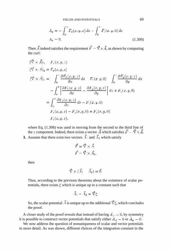
FIELDS AND POTENTIALS 69
*� � ��
�
���%� ?� �� �� �
� �
�
� �%� ?� �� �%
* � �� (1.309)
Then �* indeed satisfies the requirement �� � ��� �*, as shown by computingthe curl:
���� �*�� � ���%� ?� ��
���� �*�� � ���%� ?� ��
���� �*� � ��
�
����%� ?� ��
�%�� � � �%� ?� ���
�
�
����%� ?� ��
�?��
� ��
�
�����%� ?� ��
�%�
����%� ?� ��
�?
��� � � �%� ?� ��
�
�
�
�� �%� ?� ��
���� � � �%� ?� ��
� � �%� ?� ��� � �%� ?� �� � � �%� ?� ��
� � �%� ?� ���
where Eq. (1.308) was used in moving from the second to the third line ofthe � component. Indeed, there exists a vector �* which satisfies �� � ��� �*.
3. Assume that there exist two vectors �*� and �*� which satisfy
�� � ��� �*�
�� � ��� �*��
then
��� � �*� � �*�� � ���
Thus, according to the previous theorems about the existence of scalar po-tentials, there exists @ which is unique up to a constant such that
�*� � �*� � ��@�
So, the scalar potential �* is unique up to the additional ��@, which concludesthe proof.
A closer study of the proof reveals that instead of having * � �, by symmetryit is possible to construct vector potentials that satisfy either *� � � or *� � ��
We now address the question of nonuniqueness of scalar and vector potentialsin more detail. As was shown, different choices of the integration constant in the

70 DYNAMICS OF PARTICLES AND FIELDS
case of the scalar potential and specific choices of @ in the case of the vectorpotential all lead to valid potentials. These transformations between potentialsare simple examples of so-called gauge transformations which lead to the samephysical system via different potentials. The various possible choices that yieldthe same field are called different gauges. We will discuss the matter in detail afterdeveloping a more complete understanding of the electrodynamics expressed interms of potentials.
It is illuminating to note that the different gauges based on the non-uniquenessof the potentials, which at first may appear somewhat disturbing, can be accountedfor very naturally with the concept of an equivalence relation. An equivalencerelation is a relationship “�” between two elements of a given set that for allelements of the set satisfies
� � ��
� � A� A � �� and
� � A� A � �� � � �� (1.310)
For the case of scalar potentials, the relationship�� on the set of scalar functionsis that �� �� �� if �� � �� is a constant. For the case of vector potentials, therelationship �! on the set of vector functions is that �*� �!
�*� if and only if�*� � �*� can be written as the gradient of a scalar. In terms of gauges, in bothcases potentials are related if one can be obtained from the other via a gaugetransformation. One can quite readily verify that both these relations satisfy thecondition in Eq. (1.310).
For a fixed element �, all elements related to it constitute the equivalence classof �, denoted by ���� therefore,
��� � �%�% � ��� (1.311)
Apparently, the equivalence classes � �� of scalar potentials and � �! of vectorpotentials describe the collection of all functions >, �* satisfying �� � ��> and�� � ��� �*, respectively, which are those that can be obtained through valid gaugetransformations from one another. The concept of classes allows the descriptionof scalar and vector potentials in a very natural way; indeed, we can say thatthe scalar potential > to a vector function �� is really an equivalence class underthe relationship �� of all those functions whose divergence is �� , and the vectorpotential �* to �� is the equivalence class under �! of all those whose curl is �� �Within this framework, both scalar and vector potentials are unique, while theunderlying freedom of gauge is maintained and accounted for.
The theorems on the existence of scalar and vector potentials allow us to sim-plify the equations of electrodynamics and make them more compact. Supposewe are given �, and <, and the task is to describe the system in its entirety. UtilizingMaxwell’s equations, we can find �( and �) of the system, and for the descriptionof the electrodynamic phenomena we need a total of six components.

FIELDS AND POTENTIALS 71
By using scalar and vector potentials, we can decrease the number of variablesin the electromagnetic system. The Maxwell equation ��� �) � � implies that thereexists �* such that �) � ��� �*� On the other hand, Faraday’s law ��� �(�� �)��� ��� can then be written as
��� � �( � � �*
��
�� ��� (1.312)
This ensures that there is a scalar potential � for� �( � � �*��� that satisfies
� �( � � �*
��� ���� (1.313)
Thus, the two homogeneous Maxwell’s equations are satisfied automatically bysetting
�) � ��� �* and �( � ����� � �*
��� (1.314)
The other two inhomogeneous Maxwell equations determine the space-time be-havior of �* and � . Using the constitutive relations, �: � + �( and �) � 7 �� , weexpress these two Maxwell equations in terms of �* and �. The Ampere–Maxwelllaw takes the form
�����
7��� �*
�� �, �
�
��
+
����� � �*
��
�!
��� �*� +7�� �*
���� ��
��� � �*� +7
��
��
�� 7 �, � (1.315)
On the other hand, Coulomb’s law appears as
�� � +
����� � �*
��
�!� <
������
����� � �*� � �<
+� (1.316)
Altogether, we have obtained a coupled set of two equations. To summarize, thefollowing set of equations are equivalent to the set of Maxwell’s equations:
�) � ��� �* (1.317)
�( � ����� � �*
��(1.318)

72 DYNAMICS OF PARTICLES AND FIELDS
��� �*� +7�� �*
���� ��
��� � �*� +7
��
��
�� 7 �, (1.319)
���� ��
����� � �*� � �<
+� (1.320)
The fields �) and �( can be determined by the solutions �* and � of Eqs. (1.319)and (1.320). However, as seen in the theorems in the beginning of this section, thepotentials have the freedom of gauge in that �* is unique up to the gradient ��B ofa scalar field B, and � is unique up to a constant. For the coupled situation, it ispossible to formulate a general gauge transformation that simultaneously affects�* and � without influence on the fields. Indeed, if B is an arbitrary smooth scalarfield depending on space and time, then the transformation
�* �*� � �*� ��B (1.321)
� �� � �� �B
��(1.322)
does not affect the fields �( and �) and the two inhomogeneous equations. Equa-tion (1.317) for the magnetic field has the form
�)� � ��� �*� � ��� � �*� ��B�
� ��� �*� ��� ��B � �)�
whereas the corresponding one (Eq. 1.318) for the electric field has the form
�(� � ����� � � �*�
��� ���
��� �B
��
�� �
��� �*� ��B�
� ����� � �*
��� ���B
��� ���B
��� �(�
Furthermore, Eq. (1.319) transforms as
��� �*� � +7�� �*�
���� ��
��� � �*� � +7
���
��
�� 7 �,
� ��� �*� ������B�� +7�� �*
���� +7
����B
���
� ���
�� � �*� ���B� +7��
��� +7
��B
���
�� 7 �,
� ��� �*� +7�� �*
���� ��
��� � �*� +7
��
��
�� 7 �,�

FIELDS AND POTENTIALS 73
and Eq. (1.320) reads
����� ��
����� � �*�� � <
+
� ����� ��� �B
���
�
����� � �*� � �
�����B�
<
+
� ������
����� � �*� � <
+�
and altogether the situation is the same as before.In the gauge transformation (Eqs. 1.321 and 1.322), the freedom of choosing B
is left for the convenience depending on the problem. When �* and � satisfy theso-called Lorentz condition,
�� � �*� +7��
��� �� (1.323)
then the gauge is called the Lorentz gauge. Suppose there are solutions �*� and�� to Eqs. (1.319) and (1.320), then
�*" � �*� � ��B" (1.324)
�" � �� � �B"��
(1.325)
are also solutions as shown previously. Now,
�� � �*" � +7��"
��� �� � � �*� � ��B"� � +7
�
��
��� � �B"
��
�
� �� � �*� � +7���
��� ���B" � +7
��B"���
�
By choosing B" as a solution of
���B" � +7��B"���
� ��
�� � �*� � +7���
��
�� (1.326)
obviously the Lorentz gauge condition
�� � �*" � +7��"
��� � (1.327)

74 DYNAMICS OF PARTICLES AND FIELDS
is satisfied. Then the two inhomogeneous equations are decoupled, and we ob-tain two symmetric inhomogeneous wave equations
��� �*" � +7�� �*"
���� �7 �, (1.328)
����" � +7���"
���� �<
+� (1.329)
Another useful gauge is the Coulomb gauge, which satisfies the Coulomb con-dition
�� � �* � �� (1.330)
Supposing �*� and �� are solutions to Eqs. (1.319) and (1.320), then
�*# � �*� � ��B# (1.331)
�# � �� � �B#��
(1.332)
are also solutions. Now observe
�� � �*# � �� � � �*� � ��B#�
� �� � �*� � ���B# �
By choosing B# as a solution of
���B# � ��� � �*�� (1.333)
we obtain that
�� � �*# � � (1.334)
holds. Then the two inhomogeneous equations read
��� �*# � +7�� �*#
���� +7
����#
��� 7 �, (1.335)
����# � �<
+� (1.336)
and while there is no symmetry, it is convenient that the scalar potential �# isthe “instantaneous” Coulomb potential due to the time-dependent charge density<��%� �� .

FIELDS AND POTENTIALS 75
Sometimes a gauge where * , the � component of �*, is set to 0, is useful. Inthe proof of the existence of vector potentials we saw that it is possible to choose�* in such a way; we now assume �* does not satisfy this condition outright, andwe attempt to bring it to this form. The gauge condition in this case is
* � �� (1.337)
Supposing �*� and �� are solutions of Eqs. (1.319) and (1.320), then
�*� � �*� � ��B� (1.338)
�� � �� � �B���
(1.339)
are also solutions. In particular, we have
*� � *� ��B���
�
and by choosing B� as a solution of
�B���
� �*� � (1.340)
we obtain that, as needed,
*� � �� (1.341)
In a similar way we can of course also construct vector potentials in which the %or ? component vanishes.
We conclude the discussion of potentials with the special case of time-independent free space, in which the whole argument becomes very simple.With the constitutive relations �: � +� �( and �) � 7� �� , Maxwell’s equations are
�� � �( � �� ��� �( � �� (1.342)
�� � �) � �� ��� �) � ��� (1.343)
From the curl equations we infer that there are scalar potentials � and �$ for �(and �), respectively, such that we have
�( � ���� (1.344)
�) � ����$ � (1.345)

76 DYNAMICS OF PARTICLES AND FIELDS
Applying the divergence equations leads to Laplace equations for the electric andmagnetic scalar potential:
���� � � (1.346)
����$ � �� (1.347)
1.5.3 Boundary Value Problems
The Maxwell theory yields a variety of partial differential equations specifying thefields and potentials, and the practical determination of these requires methods tosolve PDEs. One of the important cases is the solution of the Poisson equation
���� � �<
+� (1.348)
which in the region where no charge exists reduces to the Laplace equation
���� � �� (1.349)
It is important to study under what conditions these PDEs have solutions andin what situations these solutions are unique. This question is similar in natureto the question of existence and uniqueness of solutions of ordinary differentialequations, in which case even if existence is ensured, the specification of initialconditions is usually needed to assert uniqueness. However, in the case of PDEs,the situation is more complicated since usually conditions have to be specifiednot only at a point but also over extended regions. For example, a solution of thePoisson equation for < � � � const. is given by
� � �� � �%� ?� �� ��A � �%�� ?�� ��� (1.350)
which solves the equation as long as A� � A� � A� � ����� also, it is easy toconstruct more solutions. However, apparently it is not sufficient to specify thevalue of � at just one point to determine the exact values for �� and �A� indeed,since there are five free parameters, at least five points would be needed.
Therefore, it is necessary to study in detail under what conditions solutionsexist and in what situations they are unique. Of particular interest is the case ofthe boundary value problem, in which conditions are formulated along certain“boundaries,” by which we usually mean simply connected sets that enclose theregion of interest.
As we now show, if the values of the potential are specified over an entireboundary, then any solutions of the Poisson equation are unique. Let us assumewe have given a region � which is enclosed by a simply connected boundarysurface �� We consider Green’s first identity,�
�
�����> � ��� � ��>���% �
��
��>
���� (1.351)

FIELDS AND POTENTIALS 77
where � and > are scalar functions. Green’s first identity is a direct consequenceof the Gauss theorem, �
�
�� � �* ��% �
��
�* � � ��� (1.352)
where �* is a vector function and � is the unit outward normal vector at the surface�. Choosing the special case of �* � ���>, and observing
�� � ����>� � ����> � ��� � ��>
���> � � � ��>
��
yields Green’s first identity.Now let us assume there exist two solutions �� and �� for the same bound-
ary value problem of the Poisson equation. Define the scalar function � as thedifference of �� and ��,
� � �� ���� (1.353)
Since �� and �� are both solutions,
����� � �<
+and ����� � �<
+
are satisfied inside the volume � , and we thus have
���� � � inside �� (1.354)
Now apply Green’s first identity (Eq. 1.351) to � � > � �; we have��
������� ��� � ������% �
��
���
��� (1.355)�
�
��������% �
��
���
���� (1.356)
where (Eq. 1.354) is used in moving from the left-hand side of the first equationto the left-hand side of the second equation.
Now assume that at every point on the surface �, either �� � �� or ����� �
����� holds. This entails that the right-hand side vanishes, and hence ��� �const., even everywhere inside � , and
�� � �� � const. inside �� (1.357)

78 DYNAMICS OF PARTICLES AND FIELDS
FIGURE 1.3. Method of images: A point charge put close to a conductor plane.
which means that the solution of the Poisson equation is unique up to a constant.Furthermore, if at least at one point on the boundary even� � � ��, then�� � ��
in all of � and hence the solution is completely unique.The two most important special cases for the specifications of boundary con-
ditions are those in which � is specified over the whole surface and ����� isspecified over the whole surface. The first case is usually referred to as the Dirich-let boundary condition, whereas the latter is usually called the von Neumannboundary condition. As discussed previously, however, a mixture of specifica-tion of value and derivative is sufficient for uniqueness, as long as at each point atleast one of them is given.
In some situations, it is possible to obtain solutions to boundary value problemsthrough simple symmetry arguments by suitably placing so-called image chargesto obtain the proper potential on the boundary of the problem. A simple exampleis a point charge � put in the front of an infinite plane conductor with a distance�, as shown in Fig. 1.3.
The image charge��, an equal and opposite charge, put at a distance � behindthe plane ensures that the potential on the surface assumes the proper value, andthus that the unique potential has been found. Another example is a point charge� put in the region between two infinite conductor planes which form the angle4��, as shown in Fig. 1.4.
FIGURE 1.4. Method of images: a point charge put in a region between two conductor planes ofangle ���.

FIELDS AND POTENTIALS 79
The problem is simulated by �� � � image charges put in the region out ofinterest to form mirror images. All �� charges form potential � at each edge linein the picture.
As discussed in subsequent chapters, the method of images is often practicallyuseful in order to numerically solve potential problems.


Chapter 2
Differential Algebraic Techniques
In this chapter, we discuss a technique that is at the core of further discussionsin the following chapters. Differential algebraic techniques find their origin in theattempt to solve analytic problems with algebraic means. One of the initiatorsof the field was Liouville (Ritt 1948) in connection with the problem of integrationof functions and differential equations in finite terms. It was then significantlyenhanced by Ritt (1932), who provided a complete algebraic theory of the solutionof differential equations that are polynomials of the functions and their derivativesand that have meromorphic coefficients. Further development in the field is due toKolchin (1973) and, with an eye on the algorithmic aspect, to Risch (1969, 1970,1979).
Currently, the methods form the basis of many algorithms in modern formulamanipulators, in which the treatment of differential equations and quadratureproblems calls for the solution of analytic problems with algebraic means. Otherimportant current work relying on differential algebraic methods is the practicalstudy of differential equations under algebraic constraints, so-called differentialalgebraic equations ((Ascher and Petzold 1998); (Griepentrog and Marz 1986);(Brenan, Campbell, and Petzold 1989; Matsuda 1980)).
For our purposes, we will concentrate on the use of differential algebraic tech-niques ((Berz 1986), (1986, 1987b, 1989)) for the solution of differential equa-tions and partial differential equations, in particular we discuss the efficient deter-mination of Taylor expansions of the flow of differential equations in terms ofinitial conditions. The methods developed here have taken the perturbative treat-ment of flows ��� � ����� of dynamical systems from the customary third(Brown 1979a; Wollnik, Brezina, and Berz 1987; Matsuo and Matsuda 1976;Dragt, Healy, Neri, and Ryne 1985) or fifth order (Berz, Hofmann, and Wollnik1987) all the way to arbitrary order in a unified and straightforward way. Sinceits introduction, the method has been widely utilized in a large number of newmap codes ((Makino and Berz 1996a; Berz, Hoffstatter, Wan, Shamseddine, andMakino 1996); (Berz 1992b), (1992b, 1995a); (Michelotti 1990; Davis, Douglas,Pusch, and Lee-Whiting 1993; van Zeijts and Neri 1993; van Zeijts 1993; Yan1993; Yan and Yan 1990; Iselin 1996)).
81 Copyright c� 1999 by Martin BerzAll rights of reproduction in any form reserved.

82 DIFFERENTIAL ALGEBRAIC TECHNIQUES
2.1 FUNCTION SPACES AND THEIR ALGEBRAS
2.1.1 Floating Point Numbers and Intervals
The basic idea behind this method is to bring the treatment of functions and theoperations on them to the computer in a similar way as the treatment of num-bers. In a strict sense, neither functions (e.g., those that are 6�, infinitely oftendifferentiable) nor numbers (e.g., the real .) can be treated on a computer sinceneither can in general be represented by a finite amount of information; after all,a real number “really” (pun intended) is an equivalence class of bounded Cauchysequences of rational numbers.
However, from the early days of computers we are used to dealing with num-bers by extracting information deemed relevant, which in practice usuallymeans the approximation by floating point numbers with finitely many digits.In a formal sense, this is possible since for every one of the operations on realnumbers, such as addition and multiplication, we can craft an adjoint operationon the floating point numbers such that the following diagram commutes:
�� A � . '������������� ����A � �0
�
"""""""""#
"""""""""#�
� � A�������������
' ��� �A
(2.1)
Of course, in reality the diagrams commute only “approximately,” which typicallymakes the errors grow over time.
The approximate character of these arguments can be removed by representinga real number not by one floating point number but rather by interval floatingpoint numbers providing a rigorous upper and lower bound ((Hansen ; Moore1979), (1988); (Alefeld and Herzberger 1983; Kaucher and Miranker 1984; Kear-fott and Kreinovich 1996)).
By rounding operations down for lower bounds and up for upper bounds, rig-orous bounds can be determined for sums and products, and adjoint operationscan be made such that diagram (2.1) commutes exactly. In practice, while alwaysmaintaining rigor, the method sometimes becomes somewhat pessimistic becauseover time the intervals often have a tendency to grow. This so-called dependencyproblem can be alleviated significantly in several ways, and a rather automatedapproach is discussed in (Makino and Berz 1996b).
2.1.2 Representations of Functions
Historically, the treatment of functions in numerics has been done based on thetreatment of numbers and, as a result, virtually all classical numerical algorithms

FUNCTION SPACES AND THEIR ALGEBRAS 83
are based on the mere evaluation of functions at specific points. As a consequence,numerical methods for differentiation, which offer one way to attempt to computeTaylor representations of functions, are very cumbersome and prone to inaccura-cies because of cancellation of digits, and they are not useful in practice for ourpurposes.
The success of the new methods is based on the observation that it is possible toextract more information about a function than its mere values. Indeed, attemptingto extend the commuting diagram in Eq. (2.1) to functions, one can demand theoperation ' to be the extraction of the Taylor coefficients of a prespecified order of the function. In mathematical terms, ' is an equivalence relation, and theapplication of ' corresponds to the transition from the function to the equivalenceclass comprising all those functions with identical Taylor expansion to order .
Since Taylor coefficients of order for sums and products of functions as wellas scalar products with reals can be computed from those of the summands andfactors, it is clear that the diagram can be made to commute; indeed, except for theunderlying inaccuracy of the floating point arithmetic, it will commute exactly. Inmathematical terms, this means that the set of equivalence classes of functionscan be endowed with well-defined operations, leading to the so-called truncatedpower series algebra (TPSA) ((Berz 1986), (1986, 1987b)).
This fact was utilized in the first paper on the subject (Berz 1987b), which ledto a method to extract maps to any desired order from a computer algorithm thatintegrates orbits numerically. Similar to the need for algorithms within floatingpoint arithmetic, the development of algorithms for functions followed, includ-ing methods to perform composition of functions, to invert them, to solve non-linear systems explicitly, and to introduce the treatment of common elementaryfunctions; many of these algorithms ((Berz 1999), (1999, 1991b)) will be dis-cussed later.
However, it became apparent quickly ((Berz 1988b), (1988b, 1989)) that thisrepresents only a halfway point, and one should proceed beyond mere arith-metic operations on function spaces of addition and multiplication and considertheir analytic operations of differentiation and integration. This resulted inthe recognition of the underlying differential algebraic structure and its prac-tical exploitation, based on the commuting diagrams for addition, multiplication,and differentiation and their inverses:
�� � '��������� ��-
���"""""#
"""""# ���
� � ����������
' ��� -
�� � '��������� ��-
�� �"""""#
"""""# ���
� �����������
' �� -

84 DIFFERENTIAL ALGEBRAIC TECHNIQUES
� '��������� �
�� ���
"""""#"""""# �� ���
��� �������������
' ��� ��� �
(2.2)
The theory of this approach will be developed in detail in this chapter.Of course, the question of what constitutes “information deemed relevant” for
functions does not necessarily have a unique answer. Formula manipulators, forexample, attack the problem from a different perspective by attempting to alge-braically express functions in terms of certain elementary functions linked byalgebraic operations and composition. In practice, the Achilles’ heel of this ap-proach is the complexity that such representations can take after only a few opera-tions. Compared to the mere Taylor expansion, however, they have the advantageof rigorously representing the function under consideration. Modern extensions ofthe Taylor method (Makino and Berz 1996b) have the ability to overcome this dif-ficulty by providing fully rigorous bounds for remainder terms; but these methodsgo beyond the scope of this book.
2.1.3 Algebras and Differential Algebras
Before proceeding, it is worthwhile to put into perspective a variety of differ-ent concepts that were introduced to the field in connection with the previouslydiscussed developments. We do this in parallel to establishing the scope of thefurther developments in which differential algebraic techniques will be appliedextensively.
The first and simplest structure that was introduced ((Berz 1986), (1986,1987b)) is TPSA. This is the structure that results when the equivalence classesof functions are endowed with arithmetic such that the diagrams in Eq. (2.1)commute for the basic operations of addition, multiplication, and scalar mul-tiplication. Addition and scalar multiplication lead to a vector space, and themultiplication operation turns it into a commutative algebra. In many respects,together with the polynomial algebras, this structure is an archetypal nontrivialalgebra, and in fact it can be embedded into many larger and more interestingalgebras.
TPSA can be equipped with an order, and then it contains differentials, i.e.,infinitely small numbers. This fact triggered the study of such nonarchimedeanstructures in more detail and led to the introduction of a foundation of analysis((Berz 1996), (1990a, 1994, rint)) on a larger and for such purposes much moreuseful structure, the Levi–Civita field discussed in Section 2.3.5. The Levi–Civitafield is the smallest nonarchimedean extension of the real numbers that is alge-braically and Cauchy complete, and many of the basic theorems of calculus canbe proved in a similar way as in .� Furthermore, concepts such as Delta functionsand the idea of derivatives as differential quotients can be formulated rigorously

FUNCTION SPACES AND THEIR ALGEBRAS 85
and integrated seamlessly into the theory. On the practical end, based on the latterconcept, there are also several improvements regarding methods of computationaldifferentiation ((Shamseddine and Berz 1996),(1997)).
The final concept that is connected to our methods and worth study is the tech-nique of automatic differentiation (Berz, Bischof, Griewank, Corliss, and Eds.1996; Griewank, Corliss, and Eds. 1991; Berz rint). The purpose of this disciplineis the automated transformation of existing code in such a way that derivativesof functional relationships between variables are calculated along with the orig-inal code. Besides the significantly increased computational accuracy comparedto numerical differentiation, a striking advantage of this approach is the fact thatin the so-called reverse mode it is actually possible in principle to calculate gra-dients in = variables in a fixed amount of effort; independent of =, in the optimalcase the entire gradient can be obtained with a cost equalling only a few timesthe cost of the evaluation of the original functions, in stark contrast to numericaldifferentiation which requires �= � �� times the original cost.
In practice, multivariate automatic differentiation is almost exclusively re-stricted to first order, and as such is not directly useful for our purposes. Onereason for this situation is the fact that conventional numerical algorithms avoidhigher derivatives as much as possible because of the well-known difficultieswhen trying to obtain them via numerical differentiation, which for a long timerepresented the only available approach. On the other hand, the previously men-tioned savings that are possible for linear derivatives are much harder to obtain inthe same way for higher orders.
Altogether, the challenge in automatic differentiation is more reminiscent ofsparse matrix techniques for management and manipulation of Jacobians thanof a power series technique. It is perhaps also worth mentioning that because ofthe need for code restructuring in order to obtain performance, there is a certainreluctance in the community toward the use of the word “automatic.” Mostly inorder to avoid the impression of making false pretence, the technique has recentlybeen referred to as computational differentiation.
Only very recently are other groups in computational differentiation picking upat least on second order (Abate, Bischof, Roh, and Carle 1997), but so far the onlysoftware for derivatives beyond order two listed in the automatic differentiationtool compendium (Bischof and Dilley ) is in fact the package DAFOR ((Berz1991a), (1987a, 1990c)) consisting of the FORTRAN precompiler DAPRE andthe arbitrary order DA package that is also used as the power series engine inthe code COSY INFINITY (Berz 1997a; et al. ; Makino and Berz 1999a; Berz,Hoffstatter, Wan, Shamseddine, and Makino 1996; Makino and Berz 1996a).
As alluded to previously, the power of TPSA can be enhanced by the intro-duction of derivations � and their inverses, corresponding to the differentiationand integration on the space of functions. The resulting structure, a differen-tial algebra (DA), allows the direct treatment of many questions connected withdifferentiation and integration of functions, including the solution of the ODEs��%��� � ����%� �� describing the motion and PDEs describing the fields.

86 DIFFERENTIAL ALGEBRAIC TECHNIQUES
2.2 TAYLOR DIFFERENTIAL ALGEBRAS
2.2.1 The Minimal Differential Algebra
We begin our study of differential algebraic structures with a particularly simplestructure which is of historical significance and constitutes the simplest nontrivialdifferential algebra (Berz 1989). In fact, the reals under their regular arithmeticwith a derivation � that vanishes identically trivially form a differential algebra,but it is not a very interesting one. To obtain the first nontrivial differential algebra,we have to move to .�� Let us consider the set of all ordered pairs ���� ���, where�� and �� are real numbers. We define addition, scalar multiplication and vectormultiplication as follows:
���� ��� � ���� ��� � ��� � ��� �� � ��� (2.3)
� � ���� ��� � �� � ��� � � ��� (2.4)
���� ��� � ���� ��� � ��� � ��� �� � �� � �� � ���� (2.5)
The ordered pairs with the arithmetic are called �:�� The first two operations arethe familiar vector space structure of .�� The multiplication, on the other hand,looks similar to that in the complex numbers; except here, as one sees easily,��� �� � ��� �� does not equal ���� �� but rather ��� ��. Therefore, the element
� ��� ��� �� (2.6)
plays a quite different role than the imaginary unit � in the complex numbers.The multiplication of vectors is seen to have ��� �� as the unity element and to becommutative, i.e., ���� ��� � ���� ��� � ���� ��� � ���� ���� It is also associative, i.e.,���� ��� � ����� ��� � ��� ��� � ����� ��� � ���� ���� � ��� ��� It is also distributivewith respect to addition, i.e., ���� ��� � ����� ��� � ��� ��� � ���� ��� � ���� ��� ����� ��� � ��� ��, and so the two operations � and � form a (commutative) ring.Together, the three operations form an algebra. Like the complex numbers, theydo form an extension of the real numbers; because ��� �� � �� �� � �� � � ��and ��� �� � �� �� � �� � � ��� the pairs ��� �� behave like real numbers, and thusas in 6� the reals can be embedded.
However �:� is not a field. Indeed, it can be shown that ���� ��� � �:� has amultiplicative inverse in �:� if and only if �� �� �. If �� �� � then
���� ����� �
��
���������
�� (2.7)
We also note that if �� is positive, then ���� ��� � �:� has a root
$���� ��� �
�����
����
��
�� (2.8)

TAYLOR DIFFERENTIAL ALGEBRAS 87
as simple arithmetic shows.The structure �:� plays a quite important role in the theory of real alge-
bras. All two-dimensional algebras, which are the smallest nontrivial algebras,are isomorphic to only three different kinds of algebras: the complex numbers,the so-called dual numbers in which ��� �� ���� �� � ��� ��, and the algebra �:��
In fact, this rather unique algebra has some interesting properties. One of themis that �:� can be equipped with an order that is compatible with its algebraicoperations. It is this requirement of compatibility of the order with addition andmultiplication that makes ., the field of real numbers, an ordered field. On theother hand, while many orders can be introduced on the field of complex numbers,none can be made compatible with the field’s arithmetic; we say that the complexnumbers cannot be ordered.
Given two elements ���� ��� and ���� ��� in �:�, we define
���� ��� � ���� ��� if �� � �� or ��� � �� and �� � ���
���� ��� � ���� ��� if ���� ��� � ���� ���
���� ��� � ���� ��� if �� � �� and �� � ��� (2.9)
It follows immediately from this order definition that for any two elements �� �� ���and ���� ��� in �:�� one and only one of ���� ��� � ���� ���� ���� ��� � ���� ���and ���� ��� � ���� ��� holds. We say that the order is total; alternatively, �:� istotally ordered. The order is compatible with addition and multiplication; for all���� ���� ���� ���� ��� �� � �:�, we have ���� ��� � ���� ��� �� ���� ��� ���� �� � ���� ��� � ��� ��� and ���� ��� � ���� ���; and ��� �� � ��� �� �� �� ���� ��� � ��� �� � ���� ��� � ��� ��� We also see that the order on thereals embedded in �:� is compatible with the order there.
The number � defined previously has the interesting property that it is positivebut smaller than any positive real number; indeed, we have
��� �� � ��� �� � ��� �� � �� (2.10)
We say that � is infinitely small. Alternatively, � is also called an infinitesimal ora differential. In fact, the number � is so small that its square vanishes, as shownpreviously. Since for any ���� ��� � �:� we have
���� ��� � ���� �� � ��� ��� � �� � � � ��� (2.11)
we call the first component of ���� ��� the real part and the second component thedifferential part.
The number � has two more interesting properties. It has neither a multiplica-tive inverse nor an th root in �:� for any � �. For any ���� ��� in �:�, wehave
���� ��� � ��� �� � ��� ��� �� ��� ��� (2.12)

88 DIFFERENTIAL ALGEBRAIC TECHNIQUES
On the other hand, one easily shows by induction on that
���� ���� � ���� � � ����� ��� for all ���� ��� � �:� and all � �� (2.13)
Therefore, if � has an th root ���� ��� � �:�, then
���� � � ����� ��� � ��� ��� (2.14)
from which we have simultaneously �� � � and � ����� �� � �—a contradiction,for � �. Therefore, � has no th root in �:�.
We next introduce a map � from �:� into itself, which will prove to be a deriva-tion and will turn the algebra �:� into a differential algebra.
Define � � �:� �� �:� by
����� ��� � ��� ���� (2.15)
Note that
������ ��� � ���� ���� � ���� � ��� �� � ��� � ��� �� � ���
� ��� ��� � ��� ��� � ����� ��� � ����� ��� (2.16)
and
������ ��� � ���� ���� � ���� � ��� �� � �� � �� � ��� � ��� �� � �� � �� � ���� ��� ��� � ���� ��� � ���� ��� � ��� ���� ������ ���� � ���� ��� � ���� ��� � ������ ����� (2.17)
This holds for all ���� ���� ���� ��� � �:�. Therefore, � is a derivation, andhence � �:�� �� is a differential algebra.
There is another way of introducing a derivation on �:�� which maps into thereal numbers, by setting � %����� ��� � ��� Also �%� satisfies the previous addi-tion and multiplication rules; but because it does not map �:� into itself, it doesnot introduce a differential algebraic structure on �:�� The derivation � is appar-ently connected to � %� by � � � � �%�, and hence has a resemblence to a vectorfield (Eq. 1.7).
For the purposes of beam physics, the most important aspect of �:� is that itcan be used for the automated computation of derivatives. This is based on thefollowing observation. Let us assume that we have given the values and deriva-tives of two functions � and � at the origin; we put these into the real and dif-ferential components of two vectors in �:�, which have the form ������ � �����and ������ ������� Let us assume we are interested in the derivative of the product� � �, which is given by � ���� � ���� � ���� � ������ Apparently, this value appears

TAYLOR DIFFERENTIAL ALGEBRAS 89
in the second component of the product ������ � ����� � ������ ������, whereas thefirst component of the product happens to be ���� � ����. Therefore, if two vec-tors contain the values and derivative of two functions, their product contains thevalues and derivatives of the product function. Defining the operation � � from thespace of differentiable functions to �:� via
�� � � ������ � ������ (2.18)
we thus have
�� � �� � �� � � ��� (2.19)
�� � �� � �� � � ���� (2.20)
and hence the operation closes the two upper commuting diagrams in Eq. (2.2).Similarly, the addition in �:� is compatible with the sum rule for derivatives.
In this light, the derivations of rules for multiplicative inverses (Eq. 2.7) androots (Eq. 2.8) appear as a fully algebraic derivation of the quotient and root rulesof calculus, without any explicit use of limits of differential quotients; this is asmall example of generic differential algebraic reasoning.
This observation about derivatives can now be used to compute derivatives ofmany kinds of functions algebraically by merely applying arithmetic rules on �:�,beginning with the value and derivative of the identity function. We illustrate thiswith an example using the function
��%� ��
%� ���%�� (2.21)
The derivative of the function is
� ��%� ����%��� �
�% � ���%���� (2.22)
Suppose we are interested in the value of the function and its derivative at % � .We obtain
��� �
��� � ��� � � �
��� (2.23)
Now take the definition of the function � in Eq. (2.21) and evaluate it at valueand derivative of the identity function �� �� � � �. We obtain
� ��� ��� ��
�� �� � ���� ���
�
�� �� � ���������
��
����� �����
�
�����
�
% ���
�
��
�
���� �
��
�� (2.24)

90 DIFFERENTIAL ALGEBRAIC TECHNIQUES
As can be seen, after the evaluation of the function the real part of the resultis the value of the function at % � , whereas the differential part is the value ofthe derivative of the function at % � .This result is not a coincidence. Using Eq.(2.18), we readily obtain that for all � with ���� �� � in �:�,
����� � ������� � ������ (2.25)
Thus,
���%�� �
��
%� ��%
��
�
�%� ��%�
��
�%� � ���%��
�
�%� � ���%�
� ���%��� (2.26)
Since for a real %� we have �%� � �%� �� � % � �� and ���%�� � ���%�� � ��%��,apparently
����� � ���� � � �� � ��� � (2.27)
The method can be generalized to allow for the treatment of common intrin-sic functions � like ���� � !� by setting ������� ��� � ��������� �� "#�������� !���� ��� � �� !����� �� � !�����, or more generally,
���� �� � ������ or
� ����� ���� � ������� ��������� (2.28)
By virtue of Eqs. (2.5) and (2.28), we see that any function � representableby finitely many additions, subtractions, multiplications, divisions, and intrinsicfunctions on �:� satisfies the important relationship
���%�� � ���%��� (2.29)
Therefore, for all � � . � �:�, we can write
������ � ����� � ��� � ��� (2.30)
from which we infer that ���� and � ���� are equal to the real and differential partsof ��� � ��, respectively.
Note that Eq. (2.30) can be rewritten as
��� � �� � ���� � � � � ����� (2.31)
This resembles ��%��%� � ��%���% �� ��%�, in which case the approximationbecomes increasingly better for smaller �%. Here, we choose an infinitely small

TAYLOR DIFFERENTIAL ALGEBRAS 91
�%, and the error turns out to be zero. In Section 2.3.5 we provide a more de-tailed analysis of this interesting phenomenon and at the same time obtain someinteresting new calculus.
2.2.2 The Differential Algebra �:!
In this section, we introduce a differential algebra that allows the computation ofderivatives up to order of functions in = variables. Similar to before, it is basedon taking the space 6��.!�� the collection of times continuously differentiablefunctions on .!. As a vector space over ., 6��.!� is infinite dimensional; forexample, the set of all monomials %
� is linearly independent.On the space 6��.!�� we now introduce an equivalence relation. For � and � in
6��.!�, we say � �� � if and only if ���� � ���� and all the partial derivativesof � and � agree at 0 up to order . The newly introduced relation � � apparentlysatisfies
� �� � for all � � 6��.!��
� �� � �� � �� � for all �� � � 6��.!� and
� �� � and � �� 9 �� � �� 9 for all �� �� 9 � 6��.!�� (2.32)
Thus, �� is an equivalence relation. We now group all those elements that arerelated to � together in one set, the equivalence class �� � of the function � . Theresulting equivalence classes are often referred to as DA vectors or DA numbers.Intuitively, each of these classes is then specified by a particular collection ofpartial derivatives in all = variables up to order . We call the collection of allthese classes �:!�
Now we try to carry over the arithmetic on 6 ��.!� into �:!. We observe thatif we know the values and derivatives of two functions � and �, we can infer thecorresponding values and derivatives of � � � (by mere addition) and � � � (byvirtue of the product rule). Therefore, we can introduce arithmetic on the classesin �:! via
�� � � ��� � �� � �� (2.33)
� � �� � � �� � � � (2.34)
�� � � ��� � �� � ��� (2.35)
Under these operations, �:! becomes an algebra. For each � � ��� � � � � =�, de-fine the map �� from �:! to �:! for � via
���� � �
��� � ��
�%�
�� (2.36)

92 DIFFERENTIAL ALGEBRAIC TECHNIQUES
where
���%�� � � � � %!� � %� (2.37)
projects out the �th component of the identity function. Note that th order deriva-tives of �� � �����%�� involve the product of the value of �� at the origin with� � ��st order derivatives of � at the origin. Even though we do not know thevalues of these latter derivatives at the origin, we do know the results of their mul-tiplications with the value of �� at the origin, which is �. It is easy to show that,for all � � �� � � � � = and for all �� �� ��� � �:!, we have:
����� � � ���� � ���� � � ����� (2.38)
����� � � ���� � �� � � ��� ���� � ����� �� � ���� (2.39)
Therefore, �� is a derivation for all �, and hence ��:!� ��� � � � � �!� is a differ-ential algebra. Indeed, �:! is a generalization of �:�� which is obtained as thespecial case � � and = � ��
2.2.3 Generators, Bases, and Order
Similar to the case of �:�� the differential algebra �:! also contains the realnumbers; in fact, by mapping the real number � to the class ��� of the constantfunction that assumes the value � everywhere, we see that the arithmetic on �:!
corresponds to the arithmetic on .�Next, we want to assess the dimension of �:!. We define the special numbers
�� as follows:
�� � �%� �� (2.40)
We observe that � lies in the same class as its Taylor polynomial '� of order around the origin; they have the same function values and derivatives up to order, and nothing else matters. Therefore,
�� � � �'� � � (2.41)
Denoting the Taylor coefficients of the Taylor polynomial ' � of � as �������� , wehave
'� �%�� � � � � %!� ��
���������
�������� � %�� � � � � � %�! � (2.42)
with
�������� ��
�� � � � � � ! � ����������
�%�� � � � � � �%�!(2.43)

TAYLOR DIFFERENTIAL ALGEBRAS 93
and thus
�� � � �'� � �
&' ����������
�������� � %�� � � � � � %�!
()
��
���������
�������� � ��� � � � � � ��! � (2.44)
where, in the last step, use has been made of ���A� � �����A� and �� �A� � ��� � �A��Therefore, the set ��� �� � � � �� �� � � � � =� generates �:!; that is, any elementof �:! can be obtained from � and the ��’s via addition and multiplication.Therefore, as an algebra, �:! has �= � �� generators. Furthermore, the terms��� � � � � � ��! for � � � � � � � ! form a generating system for the vec-tor space �:!� They are in fact also linearly independent since the only way toproduce the zero class by summing up linear combinations of � �
� � � � � � ��! is bychoosing all their coefficients to be zero; so the ��
� � � � � ���! actually form a basisof �:!, called the differential basis, for reasons that will become clear later. Wenow want to study how many basis elements exist and thus find the dimensionof �:! . To this end, we represent each =-tuple of numbers �� � � � � ! that satisfy� � � � � �� ! by the following unique sequence of ones and zeros:
��� �� � � � � �* +, -� times
� �� �� �� � � � � �* +, -� times
� �� � � � � �� �� �� � � � � �* +, -� times
� �� �� �� � � � � ���* +, -��������� times
(2.45)
Apparently, the value � appears a total of times, and the value � appears = times,for a total length of � =� The total number of such vectors, which is then equalto the number of basis vectors, is given by the number of ways that � can bedistributed in the � = slots; this number is given by
/�� =� ��� dim �:! �
�� =
=
��
�� =��
� =�� (2.46)
For later use, we also note that a similar argument shows that the basis vectorsbelonging to the precise order can be described by the sequence
��� �� � � � � �* +, -� times
� �� �� �� � � � � �* +, -� times
� �� � � � � �� �� �� � � � � �* +, -� times
�� (2.47)
which has length � = � � and = � � zeros, yielding the following total numberof possibilities:
��� =� �
�� = � �
= � �
�� /�� = � ��� (2.48)

94 DIFFERENTIAL ALGEBRAIC TECHNIQUES
TABLE ITHE DIMENSION OF ��� AS A FUNCTION OF � AND �, FOR �� � � �� � � � � ��
1 2 3 4 5 6 7 8 9 10
1 2 3 4 5 6 7 8 9 10 11
2 3 6 10 15 21 28 36 45 55 66
3 4 10 20 35 56 84 120 165 220 286
4 5 15 35 70 126 210 330 495 715 1,001
5 6 21 56 126 252 462 792 1,287 2,002 3,003
6 7 28 84 210 462 924 1,716 3,003 5,005 8,008
7 8 36 120 330 792 1,716 3,432 6,435 11,440 19,448
8 9 45 165 495 1,287 3,003 6,435 12,870 24,310 43,758
9 10 55 220 715 2,002 5,005 11,440 24,310 48,620 92,378
10 11 66 286 1,001 3,003 8,008 19,448 43,758 92,378 184,756
Since the number of terms up to order equals the number of terms up to order� � plus the number of terms of exact order � we have
/�� =� � /�� �� =� �/�� = � ��� (2.49)
which also follows directly from the properties of binomial coefficients.Table I gives the dimension of �:! as a function of and =, for � = �
�� � � � � ��. Note that the table clearly shows the recursive relation (Eq. 2.49).Moreover, the table is symmetric about the diagonal, which is a direct resultof the fact that the dimension of �:! , /�� =�, is symmetric in and =, i.e.,/�� =� � /�=� ��
Since �:! is finite dimensional, it cannot be a field. Otherwise, this would con-tradict Zermelo’s Theorem, which asserts that the only finite dimensional vectorspaces over . which are fields are 6 and the quaternions (in which multiplica-tion is not commutative). This will be confirmed again later by the existence ofnilpotent elements (the infinitesimals), which can have no multiplicative inverse.
Similar to the structure �:�� �:! can also be ordered (Berz 1990b). Given aDA number, we look for the terms that have the lowest sum of exponents of the �
that occurs. From all combinations of these exponents, we find the ones with thehighest exponent in ��, and from these the ones with the highest exponent of � �,and so on. The resulting combination is called the leading term and its coefficientthe leading coefficient. For example, if a DA vector has a constant part, then theconstant part is the leading term; if the constant part vanishes but the coefficientof �� is nonzero, then �� will be the leading term. We now say the DA number ispositive if its leading coefficient is positive.

TAYLOR DIFFERENTIAL ALGEBRAS 95
We conclude that if � and A are positive, then so are both � � A and � � A. Theleading term of �� A is either the leading term of � or the leading term of A, andif the leading terms are equal, the leading coefficients cannot add up to zero sincethey are both positive. The leading term of � � A is the product of the leading termof � and the leading term of A, and the leading coefficient is the product of theleading coefficients of � and A.
For � �� A in �:! , we say� � A if �� A is positive
� � A otherwise� (2.50)
Then, for any �, A in �:!, exactly one of each � � A, � � A and � � A holds.Moreover, for any �� A� � in �:!, � � A and A � � entails that � � �. Therefore,the order is total; alternatively, we say that �:! is totally ordered. Moreover, theorder is compatible with addition and multiplication, i.e., for all �� A� � in �:! wehave that
� � A �� �� � � A� �
� � A� � � � �� � � � � A � � � (2.51)
We call the order lexicographic because when comparing two numbers � andA, we look at the leading coefficient of � � A. This is equivalent to starting bycomparing the leftmost terms of � and A, and then moving right until we havefound a term in which the two numbers disagree. We also introduce the absolutevalue via
��� �� if � �
�� else� (2.52)
Note that the absolute value maps from �:! into itself, and not into . as in thenorm introduced later.
Observe that for all � � � in ., and for all � in ��� � � � � =�,� � �� � �� (2.53)
Therefore, all �� are infinitely small or infinitesimal.Now we can order the basis defined in Eq. (2.44) as follows:
�� � � � �� � �� � �� � �� � � � � � �!�� � �! � � � �� � �� � � � ��! � (2.54)
and an arbitrary element � � �� � � �:! can now be represented as an ordered/ -tuple
� � ���� ��� � � � � � �� (2.55)

96 DIFFERENTIAL ALGEBRAIC TECHNIQUES
where the �’s are the expansion coefficients of � in the basis ������� � � � �� �and are given by Eq. (2.43). Addition and multiplication rules (2.33), (2.34) and(2.35) in �:! can be reformulated as follows. For � � ���� ��� � � � � � �, A ��A�� A�� � � � � A � in �:! , and for � in ., we have:
�� A � ��� � A�� �� � A�� � � � � � � A � (2.56)
� � � � �� � ��� � � ��� � � � � � � � � (2.57)
� � A � ���� ��� � � � � � �� (2.58)
where�� �
�$��$�$�
� � A � (2.59)
It follows that an element � of �:! is an infinitesimal if and only if its firstcomponent ��� the so-called real part, vanishes. To conclude the section, wealso observe that the total number 0 �� =� of multiplications of the form � � Anecessary to compute all coefficients �� of the product is given by
0 �� =� � /�� �=� �
�� �=
�=
��
�� �=��
� ��=��� (2.60)
since the number of each combination � �� of monomials in �:! in Eq. (2.59)corresponds uniquely to one monomial in �:�!�
2.2.4 The Tower of Ideals, Nilpotency, and Fixed Points
To any element �� � � �:!, we define the depth ;��� �� as
;��� �� �
Order of first nonvanishing derivative of � �� � �� �
� � �� � � �� (2.61)
In particular, any function � that does not vanish at the origin has ;��� �� � �� Ina similar way, on the set �:
�! that describes vector functions �� � ���� � � � � ���
from .! to .�� we define
; ������� � � � � ������ � $�������
;������ (2.62)
We observe that for any �� A � �:!, we have
;�� � A� � $���;��� � ;�A�� � ��
and;��� A� $���;���� ;�A��� (2.63)

TAYLOR DIFFERENTIAL ALGEBRAS 97
In fact, except that ; never exceeds � �� it behaves like a valuation. We nowdefine the sets !� as
!� � �� � �:! �;��� ��� (2.64)
We apparently have the relation
�:! � !� ! !� ! � � � ! !� ! !��� � ���� (2.65)
All !�’s are ideals, i.e., for � � !� and any A � �:!� we have � � A � !�� whichreadily follows from Eq. (2.63). Because of Eq. (2.65), the ! �’s are often referredto as the “tower of ideals.” The Ideal !� apparently is just the collection of thoseelements that are infinitely small or zero in absolute value. An interesting propertyof the elements in !� (and hence also those in !�� !�� � � �) is that they are nilpotent.Following the multiplication rules of the depth, we see that if � � !� and hence;��� ��
;����
� �� �� � ;��� � �� (2.66)
and so indeed
���� � �� (2.67)
In particular, all differential generators �� are nilpotent. On the other hand, allelements in �:! " !� are not nilpotent, but their powers actually stay in �:! " !��indeed, they all have ;��� � �� which also entails that ;���� � ��
We now introduce a norm of the vector � in �:!� Let � have the components���� � � � � � � in the differential basis; then we set
����� � /�� =� � $% ������
���� (2.68)
We see that
����� � � if and only if � � �
��� � ��� � ��� � ����� for all real ��
By considering �� � A� ���� �A�� we see that
���� A�� ������ ��A�� (2.69)
and hence �� �� is indeed a norm. Let � � ���� � � � � � � � � � A� From the multipli-cation rule, we remember that each of the � ’s is made by summing over productsof � and A� Since there cannot be more contributions to the sum as /�� =��

98 DIFFERENTIAL ALGEBRAIC TECHNIQUES
we have � /�� =� � $% � � $% A. This entails that /�� =� � $% ��� /�� =��$% ��� �$% �A� and hence
��� � A�� ����� � ��A��� (2.70)
so the norm satisfies a Schwartz inequality.We proceed to the study of operators and prove a powerful fixed-point theorem,
which will simplify many of the subsequent arguments. Let # be an operator onthe set � � �:
�! � Then we say that # is contracting on � if for any ��� �A ��
with �� �� �A�
;�#�����#��A�� � ;�����A� (2.71)
Therefore, in practical terms this means that after application of#� the derivativesin �� and�A agree to a higher order than they did before application of #�
For example, consider the set � � !� and the operator# that satisfies C��� ���� Then,#����#�A� � ���A� � ���A� � ���A�� and thus ;�#����#�A�� �$���;���A��;���A�� ���� ;���A�, since ��A � !� and so ;���A� � ��
We also see that if we have two operators #� and #� that are contracting on� , then their sum is contracting on � because, according to Eq. (2.63),
;��#����� �#������� �#���A� �#���A���
$���;�#������#���A��� ;�#������#���A���
� $���;��� ��A�� ;��� ��A�� � ;�����A�� (2.72)
Furthermore, if the set � on which the operators act is a subset of !�, then theirproduct is also contracting.
Another important case of a contracting operator is the antiderivation � ��� �
Indeed, assume ;��� � �A� � 2� then the first nonvanishing derivatives of ��� �A areof order 2� However, after integration with respect to any variable �� the derivativesof ����A are of order 2 � �� and thus, using the linearity of the antiderivation,
;����� ��� �����A� � ;����� �����A�� � ;��� ��A� (2.73)
and thus the antiderivation operator is contracting. This will prove eminently im-portant in the study of differential equations following.
Contracting operators have a very important property—they satisfy a fixed-point theorem. Let # be a contracting operator on � � �:! that maps �into �� Then # has a unique fixed point � � � that satisfies the fixed-pointproblem
� � #���� (2.74)
Moreover, let �� be any element in �� Then the sequence
�� � #������ for � � �� �� � � � (2.75)

TAYLOR DIFFERENTIAL ALGEBRAS 99
converges in finitely many steps [in fact, at most � � �� steps] to the fixedpoint �. The fixed-point theorem is of great practical usefulness since it ensuresthe existence of a solution and, moreover, allows its exact determination in a verysimple way in finitely many steps.
The proof of the fixed-point theorem is rather simple. Consider the sequence���� � #����� We have that
;����� � ����� � ;�C�������C�����
� ;����� � ����
Because ; assumes only integer values, we thus even have ;����� � ����� ;����� � ��� � �� and hence by induction it follows that
;����� � ����� ;����� � ��� � � � � �
;��� � ��� � �� �� � ��
Because of the definition (Eq. 2.61) of ;, this entails that ���� � ����� or be-cause ���� � #�������
���� � #�������
Therefore, the fixed point has indeed been reached exactly after � � �� steps.The fixed point is also unique; if both � and �� were distinct fixed points, then;��� ��� � ;�#��� �#����� � ;��� ���� which is a contradiction.
The fixed-point theorem, and also its proof, has many similarities to its fa-mous counterpart due to Banach on Cauchy-complete normed spaces. In Ba-nach’s version, contractivity is measured not discretely via ; but continuouslyvia the norm, and it is sufficient that there exists a real � with � � � � with�#���� � #����� � � � ��� � ���� Then the resulting sequence is shown to beCauchy, and its limit is the solution. In the DA version of the fixed-point theorem,convergence happens very conveniently after finitely many steps.
Similar to the case of the Banach fixed-point theorem, the DA fixed-point theo-rem also has many useful applications. In particular, it allows for a rather straight-forward solution of ODEs and PDEs by utilizing operators that contain deriva-tions, as will be shown later.
For example, we want to utilize the fixed-point theorem to prove the quotientrule of differentiation: Given a function � and its partial derivatives of order �that satisfies ���� �� �� Then we want to determine all the partial derivatives oforder of the function ���� In DA terminology, this is equivalent to finding amultiplicative inverse of the element � � �� � � !� � �:!� Let �� � ����� Thenwe have ;�� � ��� � �� Let A � ���� �� and as demanded � � A � �� This can berewritten as ��� ��� � A� �� � A � � or
A ��
��� ��� ��� ��� � A��

100 DIFFERENTIAL ALGEBRAIC TECHNIQUES
Defining the operator# by#�A� � ��� ��� ��� � A����� we have a fixed-pointproblem. Let �� �� �� � �:!� Then we have
; �#�����#����� � ;
��� ��
��� ��� � ���
�
� $��
�;
��� ��
��
�� ;��� � ���� � �
�� ;��� � ����
and hence the operator is contracting. Thus, a unique fixed point exists, and itcan be reached in � � steps from any starting value. This method has particularadvantages for the question of efficient computation of multiplicative inverses.
In a similar but somewhat more involved example, we derive the root rule,which allows the determination of the derivatives of
�� from those of �� We
demand ���� � �� Let � � �� �� A � ��
� �� Then A� � �� Setting �� � ���� andwriting � � �� � �� and A �
��� � �A� we have ;���� � � and ;��A� � �� The
condition A� � � can then be rewritten as
�A ���� �A�
��
��� #��A�� (2.76)
The operator # is contracting on the set � � ��A�;��A� � ��� if �� and �� are in��
;�#�����#����� � ;
��
��
������ � ����
�� ;��� � ��� � ;��� � ���
� $���;��� � ���� � ��� (2.77)
Hence, the operator is contracting, and the root can be obtained by iteration infinitely many steps. Again, the method is useful for the practical computation ofroots.
2.3 ADVANCED METHODS
2.3.1 Composition and Inversion
Let us consider a function � on .! in = variables that is at least times differ-entiable. Given the set of derivatives ���� up to order of a function � from.! to .!� we want to determine the derivatives up to order of the composi-tion � Æ� � ����, and hence the class �� Æ���� According to the chain rule,the th derivatives of � Æ � at the origin can be calculated from the respectivederivatives of� at the origin and the derivatives of up to order of � at the point

ADVANCED METHODS 101
������ This implies that the mere knowledge of ���� is sufficient for this purposeif ����� � ��� on the other hand, if this is not the case, the knowledge of ���� isnot sufficient because this does not provide information about the derivatives of �at������
Since the derivatives of � are only required to order � for the practical purposesof calculating the class �� ��� it is actually possible to replace � by its Taylorpolynomial '& around����� since '& and � have the same derivatives; therefore,
�� ��� � �'& ���� (2.78)
However, since the polynomial evaluation requires only additions and multiplica-tions, and both additions and multiplications commute with the bracket operationby virtue of Eqs. (2.33) and (2.34), i.e., �� � A� � ��� � �A� and �� � A� � ��� � �A��we have
�� ��� � '&������� (2.79)
This greatly simplifies the practical computation of the composition since it nowmerely requires the evaluation of the Taylor polynomial of � on the classes ��� ��i.e., purely DA arithmetic.
It now also follows readily how to handle compositions of multidimensionalfunctions; replacing � by the function $ mapping from . ! to .!, and denotingthe Taylor polynomial of$ around����� by �'� � we have
�$ ��� � �'� ������� (2.80)
A particularly important case is the situation in which����� � ��� in this case, theTaylor polynomial �'� of $ around ����� is completely specified by the class�$ ��� This entails that we can define a composition operation in the ideal ! !
� ��:
!! via
�$ �� Æ ���� ��� �$ Æ���� (2.81)
Now we address the question of the determination of derivatives of inverse func-tions. Let us assume we are given a map� from .! to .! with ����� � �� thatis times differentiable, and let us assume that its linearization � around theorigin is invertible. Then, according to the implicit function theorem, there is aneighborhood around �� where the function is invertible, and so there is a function��� such that���� � �� Moreover,��� is differentiable to order .
The goal is to find the derivatives of ��� from those of � in an automatedway. In the DA representation, this seemingly difficult problem can be solved byan elegant and closed algorithm.

102 DIFFERENTIAL ALGEBRAIC TECHNIQUES
We begin by splitting the map� into its linear part � and its purely nonlinearpart$ � so that we have
� � � �$ � (2.82)
Composing the inverse��� with�, we obtain
���� � �� ��� � � �$ ���
��� � ��� Æ �� �$ Æ����� (2.83)
The resulting equation apparently is a fixed-point problem. Moving to equiva-lence classes, we see that the right-hand side is contracting, since
.��� Æ ����� � �$ �� Æ �%���
/� .��� Æ ����� � �$ �� Æ �&���
/� ��� Æ ��$ �� Æ �&�� � �$ �� Æ �%���� (2.84)
However, note that �$ �� � !!� , and so for any �%�� and �&�� � !!� � if �%�� and�&�� agree to order �� then �$ �� Æ �%�� and �$ �� Æ �&�� agree to order � � �because every term in �%� and �&� is multiplied by at least one nilpotent element(namely, other components from �%� and �&��� According to the fixed-point theo-rem, this ensures the existence of a unique fixed point, which can be reached atmost iterative steps. Therefore, we have developed an algorithm to determine allderivatives of up to order of��� in finitely many steps through mere iteration.Because it requires only iteration of a relatively simple operator, it is particularlyuseful for computation.
2.3.2 Important Elementary Functions
In this section, we introduce important functions on the DA �:! � In particular,this includes the functions typically available intrinsically in a computer environ-ment, such as � !, ���, and &#'. As discussed in Section 2.3.1, for any function �that is at least times differentiable, the chain rule in principle allows the compu-tation of the derivatives of order of �� at the origin, and hence ��� �� from themere knowledge of the derivatives of �� and hence �� �� as well as the derivativesof � at ������ This allows us to define
���� �� ��� ������� (2.85)

ADVANCED METHODS 103
In particular, we thus can obtain the exponential, the trigonometric functions, anda variety of other functions as
� !��� �� ��� �� !����� &#'��� ��
��� �&#'����� (2.86)
������ �� ��� ��������� "#���� ��
��� �"#������ (2.87)$
�� � ��� �
$� � for ���� positive, (2.88)
��"�
While this method formally settles the issue of the introduction of importantfunctions on �:! in a rather complete and straightforward way, it is not usefulfor computation of the previous functions in practice in an efficient and generalway. In the following, we illustrate how this can be achieved.
We observe that by the very nature of the definition of the important functionsvia Eq. (2.85), many of the original properties of the functions translate to �:!�For example, functional relationships such as addition theorems continue to holdin �:!. To illustrate this fact, we show the addition theorem for the sin function:
������ � � ���� � ������ � ��� � ������� "#���� � "#���� �������
� ������� "#����� � �"#���� �������
� ���������"#����� � �"#�������������
� ������ �� "#������ � "#���� �� ��������� (2.89)
where we have made use of the definitions of the functions on �:! as well as thefact that �� � A� � ��� � �A� for all elementary operations such as ���, and �.Obviously, other functional rules can be derived in a very analogous way.
The addition theorems for elementary functions allow us to derive convenientcomputational tools using only elementary operations on �:!� For this pur-pose, one rewrites the expression in such a way that elementary functions actonly around points for which the coefficients of their Taylor expansion are read-ily available. As discussed in Section 2.3.1, according to Eq. (2.81) this allowssubstitution of the function itself by its th order Taylor polynomial, which com-putationally requires only additions and multiplications. For example, considerthe elementary function � � ���. We split the argument function � in the class �� �into two parts, its constant part �� � ���� and its differential (nilpotent) part �� ,so that
�� � � ���� � � �� �� (2.90)

104 DIFFERENTIAL ALGEBRAIC TECHNIQUES
We then conclude
������ �� � �������� � � �� �� � ��������� "#��� �� �� � "#������� ����� �� ��
� ���������
�����
���� ��� ��
������ �"#������
�����
���� � �� ����
���� ���� (2.91)
where ��� is the largest integer that does not exceed ���The strategy for other functions is similar; for example, we use
� !��� � A� � � !���� � � !�A� (2.92)$�� � A �
��� �
0� �
A
��(for �� � �� (2.93)
&#'��� � A� � &#'���� � &#'
�� �
A
��
�(for �� � �� (2.94)
�
�� � A�
�
��� �
� � A���(for �� � �� (2.95)
and the respective Taylor expansions around � or �.It is now possible to obtain derivatives of any order of a functional depen-
dency that is given in terms of elementary operations and elementary functionsby merely evaluating in the DA framework and observing
���%�� � � � � %!�� � � ��%��� � � � � �%=�� � � ���� � � � � �!� � (2.96)
2.3.3 Power Series on �:!
We say that a sequence ���� converges in �:! if there exists a number � in �:!
such that �'����'� converges to zero in .. That is, given D � � in ., there existsa positive integer � such that '�� � �' � D for all � � �.
With the previously defined norm, �:! is a Banach space, i.e., a normed spacewhich is Cauchy complete. A sequence ���� in �:! is said to be Cauchy if foreach D � � in . there exists a positive integer � such that '�����' � D whenever� and 2 are both �. For the proof of the Cauchy completeness of �:!, we needto show that every Cauchy sequence in �:! converges in �:!.
Let ���� be a Cauchy sequence in �:! and let D � � in . be given. Then thereexists a positive integer � � � such that
'�� � ��' � D for all �� 2 �� (2.97)
According to the definition of the norm, it follows from Eq. (2.97) that
���� � ���� � D for all �� 2 � and for all � � �� �� � � � � /� (2.98)

ADVANCED METHODS 105
where ��� and ��� denote the �th components of �� and ��, respectively. Thus,the sequence ����� is a Cauchy sequence in . for each �. Since . is Cauchycomplete, the sequence ����� converges to some real number A for each �. Let
A � �A�� A�� � � � � A �� (2.99)
We claim that ���� converges to A in �:! . Let D � � in . be given. For each � thereexists a positive integer � such that ���� � A� � D�/ for all � �� Let � �$% �� � � � �� �� � � � � /�. Then ���� � A� � D�/ for all � � �� �� � � � � / andfor all � �. Therefore,
'�� � A' � D for all � �� (2.100)
and hence ���� converges to A in �:! as claimed.One particularly important class of sequences is that of power series. Let
������� be a sequence of real numbers. Then��
�� ��?�� ? ��:! is called
a power series in ? (centered at �). We say that a power series��
�� ��?� con-
verges in �:! if the sequence of partial sums, *� ���
�� ��?�, converges in
�:!.Now let
���� ��?
� be a power series in the real number ?� with real coeffi-cients and with real radius of convergence 5. We show that the series convergesin �:! if �(�?�� � 5, where (�?� denotes the real part of ?. From what we havedone so far, it suffices to show that the sequence �*�� is Cauchy in �:!, where
*� �
����
��?�� (2.101)
Let & � be given. Write ? � ?� � �?, where ?� is the constant part of ?� andhence ? � ?� � !�� Then,
����
���?� � �?�� �
����
���?� � �?�� �
������
���?� � �?��
�
����
���?� � �?�� �
������
��
���
��
���� � ���?��� �?
�
����
���?� � �?��
���
����
��� � � � �� � �?��
���
��?
?�
�� � � ���
���� � ���
��
(2.102)

106 DIFFERENTIAL ALGEBRAIC TECHNIQUES
where use has been made of the fact that �? � � for all � � . Now let 2 � & � be given. Then,
*� �*� �
������
�� � � � � � � � �� � �?��
���
�?
?�
�� � � ���
���� � ���� (2.103)
Therefore,
'*� �*�' �11111
������
�� � � � � � �� � �?��
���
��?
?�
�� � � ���
���� � ���
�11111
������
'�� � � � � � �� � �?��' �11111
���
�?
?�
�� � � ���
���� � ���
11111
������
��� � � � � � �� � �?�� ���11111
���
�?
?����� �� ���
11111 �
(2.104)
Since � � � � � � �� � � ����,
&�$� �
�� � � � � � �� � ����� &�$� �
��������� � �� (2.105)
Therefore, the first factor converges to � if �?�� � 5. Since the second factor isfinite, '*��*�' converges to �. Thus, the sequence �*�� is Cauchy in �:! for�?�� � 5. Therefore, the series converges if �?�� � 5.
Now that we have seen that the power series actually converges, the questionarises as to whether the DA vector of the power series applied to a function � isthe same as the power series applied to the DA vector �� �, which we just provedto converge. Of course, if the power series has only finitely many terms, the ques-tion is settled because the elementary operations of addition and multiplicationcommute with the class operations, and we have that �� � �� � �� � � ���, etc.However, in the case in which there are infinitely many operations, commuta-tivity is not ensured. The answer to the question can be obtained with the helpof the derivative convergence theorem.
Let � � A in . and let ������� be a sequence of real-valued functions that aredifferentiable on ��� A�. Suppose that ������� converges uniformly on ��� A� to adifferentiable function � and that �� ������ converges uniformly on ��� A� to somefunction �. Then ��%� � � ��%� for all % � ��� A�.
For the proof, let % � ��� A� and D � � in . be given. There exists a positiveinteger � such that
�� ���%� � ��%�� � D�� for all � � and for % � ��� A�� (2.106)

ADVANCED METHODS 107
from which we have
�� ����%� � � ����%�� � D�� for all % � ��� A� and ��� �� �� (2.107)
Let �� � be given. There exists �� � � such that����������� ����%�
�� %� � ����%�
���� � D��
whenever� � ��� A�� � �� % and ��� %� � �� � (2.108)
By the mean value theorem, for any integer & � and for any � �� % in ��� A�,
���� � �����%� � ��� � �������� � ���� � ��������� � �%� �� (2.109)
for some � between % and �. Using Eq. (2.107) and the fact that � � ��� A� and&� �� �,
���� � ��������� � D��� (2.110)
Combining Eqs. (2.110) and (2.109), we get
���� � �����%� � ��� � �������� � D�� � �%� ��� (2.111)
which we rewrite as���������� ���%�
�� %� ������� ����%�
�� %
���� � D��� (2.112)
Letting & ) in Eq. (2.112), we obtain that��������� ��%�
�� %� ������� ����%�
�� %
���� � D��� (2.113)
Using Eqs. (2.106), (2.108), and (2.113), we finally obtain that��������� ��%�
�� %� ��%�
���� ��������� ��%�
�� %� ������� ����%�
�� %
�����
����������� ����%�
�� %� � ����%�
����� ��� ����%� � ��%���
� D�� � D�� � D�� � D� (2.114)
Since Eq. (2.114) holds whenever � � ��� A� and � � ��� %� � �� , we concludethat � ��%� � ��%�. This finishes the proof of the theorem.

108 DIFFERENTIAL ALGEBRAIC TECHNIQUES
We next try to generalize the previous theorem to higher order derivatives:Let ������� be a sequence of real-valued functions that are times differentiableon ��� A�. Suppose that ������� converges uniformly on ��� A� to an times dif-
ferentiable function � and that �� ��� ���� converges uniformly on ��� A� to some
function ��, � � �� �� � � � � . Then, ���%� � � ���%� for all % � ��� A� and for all� � �� �� � � � � .
The proof of the statement follows by induction on . It is true for � � be-cause it directly follows from the previous theorem. Assume it is true for � ,and show that it will be true for � ��. Therefore, if ������� is a sequence ofreal-valued functions that are times differentiable on ��� A�, ������� converges
uniformly on ��� A� to a times differentiable function � , and �� ��� ���� converges
uniformly on ��� A� to some function ��, � � �� �� � � � � , then ���%� � � ���%�for all % � ��� A� and for all � � �� �� � � � � . Now let ������� be a sequence ofreal-valued functions that are � � �� times differentiable on ��� A�. Suppose that������� converges uniformly on ��� A� to a � � �� times differentiable function
� and that �� ��� ���� converges uniformly on ��� A� to some function ��, � �
�� �� � � � � ��. Then ���%� � � ���%� for all % � ��� A� and for all � � �� �� � � � � by the induction hypothesis. Furthermore, applying the previous theorem to thesequence �� �
� ����, we obtain that ����%� � � ����%� for all % � ��� A�. There-fore, ���%� � � ���%� for all % � ��� A� and for all � � �� �� � � � � � �. Thus, thestatement is true for � � �. Therefore, it is true for all .
The two previous results are readily extendable to sequences of real-valuedfunctions on .!, in which derivatives are to be replaced by partial derivatives.
We can now apply the result to the question of convergence of power seriesof DA vectors to the DA vector of the power series. As shown previously, thepower series of DA vectors converges in the DA norm within the classical radiusof convergence. This entails that all its components, and hence the derivatives,converge uniformly to the values of the limit DA vector. Hence, according to theprevious theorem, this limit contains the derivatives of the limit function.
2.3.4 ODE and PDE Solvers
Historically, the main impetus for the development of differential algebraic tech-niques were questions of quadrature and the solution of ordinary differential equa-tions. In our case, the direct availability of the derivations � and their inverses��� allows to devise efficient numerical integrators of any order.
One such method is based on the common rewriting of the ODE as a fixed-point problem by use of
�� � *���� � �� �
� �
��
������ ������� (2.115)

ADVANCED METHODS 109
Utilizing the operation ���!�� for the integral, the problem readily translates intothe differential algebra �:!��, where besides the = position variables, there is anadditional variable ��.
As shown in Eq. (2.73), the operation ���!�� is contracting. Since
;�������� ���� ������� �
��� ;���� � ����� (2.116)
it follows that
;�*������*������ � ;���� � ����� (2.117)
and hence the operator * on �:! is contracting. Thus, there exists a unique fixedpoint, which moreover can be reached in at most � � steps from any startingcondition. Thus, iterating
��� � �� (2.118)
����� � * ����� for � � �� �� � � � � � � (2.119)
yields the exact expansion of �� in the = variables and the time � to order � Theresulting polynomial can be used as an th order numerical integrator by insertingan explicit time step.
It is interesting that the computational expense for this integrator is actuallysignificantly lower than that of a conventional integrator. In the case of a con-ventional integrator, the right-hand side has to be evaluated repeatedly, and thenumber of these evaluations is at least equal to the time step order and sometimesnearly twice as much, depending on the scheme. The DA integrator requires ��iterations and hence � � evaluations of the right-hand side, but since in the��� ��st step only the �th order will be determined exactly, it is sufficient to per-form this step only at order �. Since the computational expense of DA operationsincreases quickly with order, by far the most important contribution to time comesfrom the last step. In typical cases, the last step consumes more than two-thirdsof the total time, and the DA integrator is about one order of magnitude fasterthan a conventional integrator.
For ODEs that are simultaneously autonomous and origin preserving, i.e.,time independent and admitting ����� � �� as a solution, another even more effi-cient method can be applied. For a given function on phase space � ���� �� � accord-ing to Eq. (1.7), the time derivative along the solution of any function � is givenby
�
��� ���� �� � �� � ��� �
�
��� � �� ��
The operator �� , the vector field of the ODE, also allows computation of higherderivatives via ������ � � �
���. This approach is well known (Conte and de Boor

110 DIFFERENTIAL ALGEBRAIC TECHNIQUES
1980) and in fact is even sometimes used in practice to derive analytical low-orderintegration formulas for certain functions �� . The limitation is that unless �� is verysimple, it is usually impossible to compute the repeated action of �� analytically,and for this reason this approach has not been very useful in practice. However,using the differential algebras �:! , and in particular the �� operators which dis-tinguish them from ordinary algebras, it is possible to perform the required opera-tions easily. To this end, one just evaluates �� in �:! and uses the ��s to computethe higher derivatives of �.
If the Taylor expansion of the solution in time � is possible, we have for thefinal coordinates ���
��� �
���
� � ��
���� (2.120)
where � is the identity function.If � and � are not explicitly time dependent, the time derivative part vanishes for
all iterations ���� Furthermore, if �� is origin preserving, then the order that is lost
by a plain application of �� in the gradient is restored through the multiplication;for the derivatives up to order of �� � ���� only the derivatives of up to order� � of �� � are important. This means that with one evaluation of ��� the powersof the operator �� can be evaluated to any order directly within DA for any .Using it for � � ��� the components of the vector ��� we obtain an integrator ofadjustable order.
While for general functions, it is not a priori clear whether the series in theso-called propagator converges, within the framework of �:! this is always thecase, as we will now show. Because of the Cauchy completeness of �:! withrespect to the norm on �:!� it is sufficient to show that
�����
��
����� � for � ) and for all 2� (2.121)
Using the definition of the norm (Eq. 2.68), the triangle inequality (Eq. 2.69), andthe Schwarz inequality (Eq. 2.70), we first observe that
�� �� ��� �� �11111
!���
�� � �����11111
!���
' �� � �����'
!�
��
������ � ����� �� 6 � ����� ��� (2.122)

ADVANCED METHODS 111
where the factor 6 ���
�� ������ is independent of ���� Thus,11111�����
��
�����
11111 �����
11111
��
�����
11111 '���' ������
6
��� (2.123)
However, since the real-number exponential series converges for any argument 6�
the partial sum����
� 6��� tends to zero as � ) for all choices of 2�This method is the computationally most advantageous approach for au-
tonomous, origin-preserving ODEs. In practice, one evaluation of the right-handside �� is required, and each new order requires merely one derivation and onemultiplication per dimension. For complicated functions ��� the actual computa-tional expense for each new order is only a small multiple of the cost of evaluationof ��� and hence this method is most efficient at high orders and large time steps. Inpractical use in the code COSY INFINITY, step sizes are fixed and orders adjusteddynamically, typically falling in a range between �� and ��
To conclude, we address the question of the solution of PDEs. Similar to thefixed point ODE solver, it is also possible to iteratively solve PDEs in finitelymany steps by rephrasing them in terms of a fixed-point problem. The detailsdepend on the PDE at hand, but the key idea is to eliminate differentiation withrespect to one variable by integration. For example, consider the general PDE�����%������%� � � A��� �?�A����?� � � �������������� � � �� where ��A� and � are functions of %, ?, and �� The PDE is rewritten as
� � � ��� ���
�
A�
2�A�
�
�?�
�������
���
���A�
�
�%
���
�
�%�
��
��A�
�
��
���
�
���
��3�
The equation is now in fixed-point form. Now assume the derivatives of � and����? with respect to % and � are known in the plane ? � �� Then the right-handside is contracting, and the various orders in ? can be iteratively calculated bymere iteration.
2.3.5 The Levi-Civita Field
We discuss in this section a very useful extension of DAs, a field that was discov-ered first by Levi-Civita, upon which concepts of analysis have recently been de-veloped (Berz 1994). The results obtained are very similar to the ones in nonstan-dard analysis; however, the number systems required here can be constructed di-rectly and described on a computer, whereas the ones in nonstandard analysis areexceedingly large, nonconstructive (in the strict sense that the axiom of choice isused and in a practical sense), and require quite a machinery of formal logic for
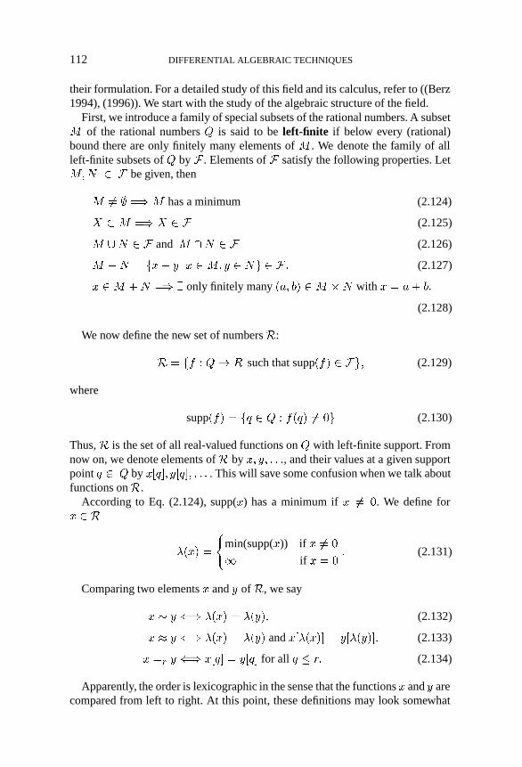
112 DIFFERENTIAL ALGEBRAIC TECHNIQUES
their formulation. For a detailed study of this field and its calculus, refer to ((Berz1994), (1996)). We start with the study of the algebraic structure of the field.
First, we introduce a family of special subsets of the rational numbers. A subset� of the rational numbers � is said to be left-finite if below every (rational)bound there are only finitely many elements of � . We denote the family of allleft-finite subsets of � by * . Elements of * satisfy the following properties. Let��/ � * be given, then
� �� + ��� has a minimum (2.124)
E �� �� E � * (2.125)
� ,/ � * and � -/ � * (2.126)
� �/ � �%� ?� % ��� ? � /� � * � (2.127)
% �� �/ �� . only finitely many ��� A� �� �/ with % � �� A�
(2.128)
We now define the new set of numbers/:
/ � �� � � . such that supp��� � *�� (2.129)
where
supp��� � �� � � � ���� �� �� (2.130)
Thus,/ is the set of all real-valued functions on � with left-finite support. Fromnow on, we denote elements of/ by %� ?� � � �, and their values at a given supportpoint � � � by %���� ?���� � � � . This will save some confusion when we talk aboutfunctions on/.
According to Eq. (2.124), supp(%) has a minimum if % �� �. We define for% � /
;�%� �
min(supp(%)) if % �� �
) if % � �� (2.131)
Comparing two elements % and ? of/, we say
% � ? 0� ;�%� � ;�?�� (2.132)
% � ? 0� ;�%� � ;�?� and %�;�%�� � ?�;�?��� (2.133)
% �% ? 0� %��� � ?��� for all � �� (2.134)
Apparently, the order is lexicographic in the sense that the functions % and ? arecompared from left to right. At this point, these definitions may look somewhat

ADVANCED METHODS 113
arbitrary, but after having introduced order on /, we will see that ; describes“orders of infinite largeness or smallness”, the relation “�” corresponds to agree-ment of order of magnitude, whereas the relation “�” corresponds to agreementup to an infinitely small relative error.
We define addition on/ componentwise: For %� ? � /, and � � �,
�%� ?���� � %��� � ?���� (2.135)
We note that the support of %�? is contained in the union of the supports of % and? and is thus itself left-finite by Eq. (2.126) and (2.125). Therefore, % � ? � /,and thus/ is closed under the addition defined previously.
Multiplication is defined as follows: For %� ? � /, and � � �,
�% � ?���� ��
����� �������
%���� � ?����� (2.136)
Note that supp�% � ?� � supp�%� � supp�?�; hence according to Eq. (2.127),supp�% � ?� is left-finite. Thus % � ? � /. Note also that left-finiteness of thesupports of/ numbers is essential for the definition of multiplication; accordingto Eq. (2.128), for any given � � �, only finitely many terms contribute to thesum in the definition of the product.
With the addition and multiplication defined previously, �/��� �� is a field.The only nontrivial step in the proof of the previous statement is the proof ofthe existence of multiplicative inverses of nonzero elements. For this, we need toinvoke the fixed-point theorem.
To show that the new field is an extension of the field of real numbers, define amap � � . � / by
��%���� �
% if � � �
� otherwise� (2.137)
Then � “embeds” . into/ (� is one-to-one, ��%�?� � ��%����?� and ��%�?� ���%� � ��?��.
Regarded as a vector space over .,/ is infinite dimensional. With the multi-plication defined previously,/ is an algebra. Furthermore, if we define an opera-tion � � / � / by
��%���� � �� � �� � %�� � ��� (2.138)
then � is a derivation and �/��� �� �� a differential algebra because � can easilybe shown to satisfy
��%� ?� � �%� �?

114 DIFFERENTIAL ALGEBRAIC TECHNIQUES
and
��% � ?� � ��%� � ? � % � ��?�� for all %� ? � /� (2.139)
We define an order on / by first introducing a set of positive elements, /�.Let % � / be nonzero; then,
% � /� 0� %�;�%�� � �� (2.140)
For % and ? in/,
% � ? 0� %� ? � /�
% � ? 0� ? � %� (2.141)
Then, the order is total and compatible with addition and multiplication in theusual way.
Having introduced an order on/, we define the number � as follows:
���� �
2� if � � �� if � �� �
� (2.142)
Then, according to the order defined previously,
� � � � � for all positive � � .� (2.143)
Hence, � is infinitely small. Moreover, it is easy to show that for all � � ��
����� �
2� if � � �� if � �� �
� (2.144)
It follows directly from the previous equation that
�� is infinitely small 0� � � �
�� is infinitely large 0� � � �� (2.145)
Having infinitely small and infinitely large numbers,/ is nonarchimedean.We introduce an absolute value on/ in the natural way:
�%� �% if % �
�% if % � �� (2.146)
/ is Cauchy complete with respect to this absolute value, i.e., every Cauchysequence in/ converges in/.

ADVANCED METHODS 115
Let �%�� be a Cauchy sequence in/; let � � � be given and let be such thatthe terms of the Cauchy sequence do not differ by more than D � � ��� from on. Define %��� �� %����. Then �%�� converges to %. Since the limit % agrees withan element of the sequence to the left of any �, its support is left-finite and thus% � /.
We return to the fixed-point theorem, which proves to be a powerful mathe-matical tool for the detailed study of/: Let � � / / be a function defined onan interval � around the origin such that ���� � � , and let � be contractingwith an infinitely small contraction factor, then � has a unique fixed point in � .
The proof is very similar to the Banach space case. One begins with an arbitraryelement %� and defines %�� � ��%�. The resulting sequence is Cauchy andconverges by the Cauchy completeness of/. Then, % � &�$� � %� is the fixedpoint of � .
Now let E � / be nonzero and show that E has a multiplicative inverse in/.Write E � %� � �% � ��� %�,where %� is real, % is infinitely small, and � � ;�E�.Since %� � �% has the inverse %��� � ��%, it suffices to find an inverse to �� � %�.Write the inverse as �� � ?�. Then we have
� � �� � %� � �� � ?�
� � � %� ? � % � ?�Thus,
? � �%� % � ?� (2.147)
This is a fixed-point problem for ? with the function ��?� � �% � % � ? and� � �� � / � ;��� � ��. Since % is infinitely small, ? is infinitely small byEq. (2.147). Thus any solution ? to Eq. (2.147) must lie in � . Also, since % isinfinitely small, � is contracting with an infinitely small contraction factor. Thefixed-point theorem then asserts the existence of a unique fixed point of � in �and thus in/.
The fixed-point theorem can also be used to prove the existence of roots of pos-itive numbers in/ and to prove that the structure 1 obtained from/ by adjoiningthe imaginary unit is algebraically closed (Berz 1994).
The algebraic properties of/ allow for a direct introduction of important func-tions, such as polynomials, rational functions, roots, and any combination thereof.Besides these conventional functions,/ readily contains delta functions. For ex-ample, the function
��%� ��
�� � %�(2.148)
assumes the infinitely large value ��� at the origin, falls off as �%� gets larger, isinfinitely small for any real %, and becomes even smaller for infinitely large (inmagnitude) %.

116 DIFFERENTIAL ALGEBRAIC TECHNIQUES
For the scope of this book, however, it is more important to study the extensibil-ity of the standard functions, in particular those representable by power series. Forthis purpose, we study two kinds of convergence. The first kind of convergenceis associated with the absolute value defined in Eq. (2.146) and is called strongconvergence. The second kind of convergence is called weak convergence; wesay that the sequence �%�� converges weakly to the limit % � / if for all � � �,%���� � %��� as � ). Therefore, weak convergence is componentwise. Itfollows from the definitions that strong convergence implies weak convergence tothe same limit. Weak convergence does not necessarily imply strong convergence,however. It is the weak convergence that will allow us to generalize power seriesto/.
Let�
��%� be a power series with real coefficients and conventional radius
of convergence 5. Then�
��%� converges weakly for all % with �(�%�� � 5 to
an element of /. This allows the automatic generalization of any power serieswithin its radius of convergence to the field /. Therefore, in a simple way, thereis a very large class of functions readily available. In particular, this includes allthe conventional intrinsic functions of a computer environment.
Let � be a function on a subset � of /. We say � is differentiable withderivative � ��%� at the point % �� if for any D � � � / there exists a Æ � � � /with Æ�D not infinitely small such that
������%��%�� ��%�
�%� � ��%�
���� � D (2.149)
for all �% with %��% �� and ��%� � Æ. Therefore, this definition very muchresembles the conventional differentiation, with an important difference being therequirement that Æ not be too small. This restriction, which is automatically sat-isfied in archimedean structures (e.g., .), is crucial to making the concept ofdifferentiation in/ practically useful.
The usual rules for sums and products hold in the same way as in the realcase, with the only exception that factors are not allowed to be infinitely large.Furthermore, it follows that if � coincides with a real function on all real pointsand is differentiable, then so is the real function, and the derivatives agree at anygiven real point up to an infinitely small error. This will allow the computationof derivatives of real functions using techniques of/.
A very important consequence of the definition of derivatives is the fundamen-tal result: Derivatives are differential quotients up to an infinitely small error.
Let �% �� � be a differential, i.e., an infinitely small number. Choose D � �infinitely small such that ��%��D is also infinitely small. Because of differentia-bility, there is a Æ � � with Æ�D at most finite such that the difference quotientdiffers from the derivative by an infinitely small error less than D for all �% with��%� � Æ. However, since Æ�D is at most finite and ��%��D is infinitely small,��%��Æ is infinitely small, and in particular ��%� � Æ. Thus, �% yields an in-finitely small error in the difference quotient from the derivative.

ADVANCED METHODS 117
This elegant method allows the compututation of the real derivative of any realfunction that has already been extended to the field / and is differentiable there.In particular, all real functions that can be expressed in terms of power series com-bined in finitely many operations can be conveniently differentiated. However, italso works for many other cases in which the DA methods fail. Furthermore, itis of historical interest since it retroactively justifies the ideas of the fathers ofcalculus of derivatives being differential quotients. It is worth pointing out thatthe computation of the derivatives as the real parts of difference quotients corre-sponds to the result in Eq. (2.31), except that division by � is impossible there,leading to the different form of the expression.
Equivalent results to the intermediate value theorem, Rolle’s theorem, and Tay-lor’s theorem can be proved to hold in /. For more details, see ((Berz 1994),(1992a)).
The last result we mention here is the Cauchy point formula. Let � ���� ��� � ���
be a power series with real coefficients. Then the function isuniquely determined by its value at a point ���9, where 9 is an arbitrary nonzeroinfinitely small number. In particular, if we choose 9 � �, we have
���� � �� ����
��� (2.150)
from which we readily obtain a formula to compute all the � ’s:
� � ���� � ������ (2.151)
This formula allows the computation of derivatives of any function which canbe written as a power series with a nonzero radius of convergence; this includesall differentiable functions obtained in finitely many steps using arithmetic andintrinsic functions.
Besides allowing illuminating theoretical conclusions, the strength of the Levi-Civita numbers is that they can be used in practice in a computer environment.In this respect, they differ from the nonconstructive structures in nonstandardanalysis.
Implementation of the Levi-Civita numbers is not as direct as that of the DAsdiscussed previously since / is infinite dimensional. However, since there areonly finitely many support points below every bound, it is possible to pick anysuch bound and store all the values of a function to the left of it. Therefore, eachLevi-Civita number is represented by these values and the value of the bound.
The sum of two such functions can then be computed for all values to the leftof the minimum of the two bounds; therefore, the minimum of the bounds is thebound of the sum. In a similar way, it is possible to find a bound below whichthe product of two such numbers can be computed from the bounds of the twonumbers. The bound to which each individual variable is known is carried alongthrough all arithmetic.


Chapter 3
Fields
For the study of transfer maps of particle optical systems, it is first necessaryto undertake a classification of the possible fields that can occur. All fields aregoverned by Maxwell’s equations (1.284, 1.285, 1.286, 1.287), which in SI unitshave the form
�� �) � �, ��� �� � � �� �:
��
�� �: � <� ��� �( � �� �)
��
In the case of particle optics, we are mostly interested in cases in which thereare no sources of the fields in the region where the beam is located, and so inthis region we have < � � and � � ��. Of course, any beam that is present wouldrepresent a < and a � , but these effects are usually considered separately.
In the following, we restrict our discussion to time-independent situations andneglect the treatment of elements with quickly varying fields including cavities.This limitation in very good approximation also includes slowly time-varyingfields such as the magnetic fields that are increased during the ramping of a syn-chrotron. In this case, Maxwell’s equations simplify to
�� �) � � , ��� �� � ��
�� �: � � , ��� �( � ��� (3.1)
where �) � 7�� and �: � +� �(� Because of the vanishing curl, we infer that byvirtue of Eq. (1.300), �) and �( have scalar potentials �' and �( such that
�( � ����' and �) � ����( � (3.2)
Note that here even the magnetic field is described by a scalar potential and notby the vector potential �* that always exist. From the first and third equations, weinfer that both scalar potentials �' and �( satisfy the Laplace equation, and thus
��'�( � �� (3.3)
119 Copyright c� 1999 by Martin BerzAll rights of reproduction in any form reserved.

120 FIELDS
In order to study the solutions of Laplace’s equations for the electric and magneticscalar potentials, we discuss two special cases, each of which will be treated in acoordinate system most suitable for the problem.
3.1 ANALYTIC FIELD REPRESENTATION
3.1.1 Fields with Straight Reference Orbit
The first major case of systems is those that have a straight reference axis. Inthis case, there is no need to distinguish between particle optical coordinates andCartesian coordinates, and in particular there is no need to transform Laplace’sequation into a new set of coordinates. Many elements with a straight referenceorbit possess a certain rotational symmetry around the axis of the reference orbit,and it is most advantageous to describe the potential in cylindrical coordinateswith a “� axis” that coincides with the reference orbit. We first begin by expandingthe � and � components of the potential in Taylor and Fourier series, respectively;the dependence on the cylindrical “�” coordinate, which here coincides with theparticle optical coordinate , is not expanded. Therefore,
� �
����
����
���� �� "#� �2�� F���� ��� (3.4)
In cylindrical coordinates, the Laplace Equation has the form
�� ��
�
�
��
����
��
��
�
�����
����
���
��� �� (3.5)
inserting the Fourier–Taylor expansion of the potential, we obtain
�� ��
�
�
��
����
��
��
�
�����
����
���
��
��
�
�
��
����
����
���� "#� �2�� F���� ���
�
��
��
����
����
���� "#� �2�� F�����2�
���
�
����
����
� ����� �� "#� �2�� F���� �
�

ANALYTIC FIELD REPRESENTATION 121
�
����
����
���� "#� �2�� F���� ������
�����
����
���� "#� �2�� F���� 2�����
�
����
����
� ������� �� "#� �2�� F������ �
���
We note that in the first term, it is possible to let the sum start at � � � since thereis no contribution because of the factor � �� Furthermore, using the convention thatthe coefficient ������ vanishes for negative indices, we obtain
�� �
������
4���� �� "#� �2�� F����
�� � 2�
��� ��
����� �� "#� �2�� F������5����� (3.6)
We begin the analysis by studying the case � � �� Apparently, ���� and F���can be chosen freely because the factor �� � � 2�� vanishes. Furthermore, since� ��
����� �� vanishes for all 2 because of the convention regarding negative indices,we infer ���� � � for 2 ��
By induction over �, we now show that ������ 2 � for all cases in which� � 2� Apparently the statement is true for � � �� Now let us assume that thestatement is true up to � � �� If � � 2� then � � � � 2� and thus � ��
����� �� � �.Since ��� � 2�� �� � and "#� �2�� F���� �� � for some � because 2 �� �� thisrequires ���� �� 2 � for � � 2. Thus, the infinite matrix ���� is strictly lowertriangular.
We now study the situation for different values of 2� We first notice that for all2, the choices of
������ and F��� are free (3.7)
because � ������� �� � � by the previous observation, and �� � � 2�� � � because
� � 2� Next we observe that the value �������� must vanish because ���� 2�� ���� but � ��
����� �� 2 � because of the lower triangularity. Recursively, we evenobtain that
������������������ � � � vanish. (3.8)
On the other hand, for � � 2 � �, we obtain that F ����� � F���� and �������� is

122 FIELDS
uniquely specified by ������. Applying recursion, we see that in general
F��� � F������ F������
and
��������� ��
������ ��6�
��
��2�
� � �2� �8��� � (3.9)
We now proceed with the physical interpretation of the result. The number2 is called the multipole order because it describes how many oscillations thefield will experience in one �4 sweep of �. The free term � ����� is called themultipole strength, and the term F��� is called the phase. Apparently, frequency 2and radial power � are coupled: The lowest order in � that appears is 2, and if themultipole strength is dependent the powers 2� �� 2 � �� � � � will also appear.
For a multipole of order 2� the potential has a total of �2 maxima and minima,and is often called a ��-pole. Often, Latin names are used for the �2 poles:
2 Leading term in � Name
� ������ "#� �F����
� ������ "#� ��� F���� � Dipole
� ������ "#� ���� F���� �� Quadrupole
������ "#� ��� F���� �� Sextupole
� ������ "#� ���� F���� �� Octupole
� ������ "#� ���� F���� �� Decapole
In many cases, it is very important to study the Cartesian (and hence alsoparticle optical) form of the fields of the elements. The case � � � with � ����� "#� ��� F���� � is quite trivial; for F�� � �� we obtain � � ���� � %� cor-responding to a uniform field in % direction, and for another important subcaseF�� � �4��� we obtain � � ���� � ?� a uniform field in ? direction.
The case � � � has � � ���� "#� ���� F��� ��. Particularly important in
practice will be the subcases F�� � � and F�� � �4��� In the first case, we get
� � ���� "#� ���� �� � ����
"#�� �� ���� �
���
� ����
%� � ?�
�� (3.10)
and in the second case we have
� � ���� "#� ���� 4��� �� � ���� �� ���� "#��� ��
� ���� ��%?� � (3.11)

ANALYTIC FIELD REPRESENTATION 123
All other angles F�� lead to formulas that are more complicated; they can be ob-tained from the ones here by subjecting the %� ? coordinates to a suitable rotation.This again leads to terms of purely second order.
Because the potential is quadratic, the resulting fields �( or �) are linear. In-deed, the quadrupole is the only -independent element that leads to linear mo-tion, similar to that in glass optics, and thus has great importance. In the electriccase, one usually chooses F��� � �� resulting in the fields
(� � ������ � % (3.12)
(� � ����� � ?� (3.13)
Therefore, different from the case of glass optics, the motion cannot be rotation-ally symmetric: If there is focusing in the % direction, there is defocusing in the ?direction and vice versa. This effect, completely due to Maxwell’s equations, per-haps the biggest “nuisance” in beam physics: If one uses piecewise -independentparticle optical elements, the horizontal and vertical planes are always differentfrom each other.
To make an electrostatic device that produces a quadrupole field, it is bestto carve the electrodes along the equipotential surfaces and utilize the fact thatif “enough” boundary conditions are specified, the field is uniquely determinedand must hence be as specified by the formula used to determine the equipoten-tial surfaces in the first place. Therefore in practice, the electrodes of an electricquadrupole often appear as shown in Fig. 3.1.
In the magnetic case, one indeed chooses F��� � �4��� resulting in
)� � ����� � ? (3.14)
)� � ����� � %� (3.15)
FIGURE 3.1. The equipotential surfaces of a quadrupole.

124 FIELDS
and examining the Lorentz forces that a particle moving mostly in -directionexperiences, we see that if there is focusing in % direction, there is defocusing in? direction and vice versa.
To study higher orders in �� let us consider the case � � . For F��� � �� weobtain
� � ���� "#� ��� �� � ���� �"#�� "#� ��� ���� ��� ��� ��
� ����
%�� "#� ��� ?�� ��� ��
�� ����
%� � %?�
�� (3.16)
In this case, the resulting forces are quadratic and are thus not suitable for af-fecting the linear motion; however, we later will show that they are indeed veryconvenient for the correction of nonlinear motion, and they even have the featureof having no influence on the linear part of the motion! Another important casefor F��� is F��� � �4��� in which case one can perform a similar argument andagain obtain cubic dependencies on the position.
For all the higher values of 2� corresponding to octupoles, decapoles, duode-capoles, etc., the procedure is very similar. We begin with the addition theoremfor "#��2�� or ����2��� and by induction it can be seen that each of these consistsof terms that have a product of precisely 2 cosines and sines. Since each of theseterms is multiplied with ��� each cosine multiplied with one � translates into an %�and each sine multiplied with one � translates into a ?� the end result is always apolynomial in % and ? of exact order 2�
Because of their nonlinear field dependence, these elements will prove to haveno effect on the motion up to order 2�� and thus allow one to selectively influencethe higher orders of the motion without affecting the lower orders. Also, if it isthe crux of particle optical motion that the horizontal and vertical linear motioncannot be affected simultaneously, it is its blessing that the nonlinear effects canbe corrected order by order.
In the case in which there is no dependence, the potential terms that we havederived are the only ones; under the presence of �-dependence, as shown inEq. (3.9), to the given angular dependence there are higher order terms in �, thestrengths of which are given by the derivatives of the multipole strength � ����The computation of their Cartesian form is very easy once the Cartesian form ofthe leading term is known because each additional term differs from the previousone by only the factor of �� � �%� � ?���
In practice, of course, dependence is unavoidable: The field of any part-icle optical element has to begin and end somewhere, and it usually does thisby rising and falling gently with � entailing dependence. This actually entailsanother crux of particle optics: Even the quadrupoles, the “linear” elements, havenonlinear effects at their edges, requiring higher order correction. The correctiveelements in turn have higher order edge effects, possibly requiring even higherorder correction, etc.
Although without dependence the case 2 � � corresponding to full rotationalsymmetry was not very interesting, if we consider dependence, it actually offers

ANALYTIC FIELD REPRESENTATION 125
a remarkably useful effect. While there is no � dependence in the leading term,the contributions through the derivatives of ������ entail terms with an � depen-dence of the form ��� ��� � � �. Of these, the �� terms will indeed produce linear,rotationally symmetric fields similar to those in the glass lens. Unfortunately, inpractice these fields are restricted to the entrance and exit fringe field regions andare comparatively weak; furthermore, there are usually quite large nonlinearities,and these devices are usually used mostly for low-energy, small emittance beams,like those found in electron microscopes.
3.1.2 Fields with Planar Reference Orbit
In the case of the straight reference orbit, Maxwell’s equations entail a very cleanconnection between rotational symmetry and radial potential. As one may ex-pect, in the case of a nonstraight reference orbit, this is no longer the case; in thissituation, Maxwell’s equations have a rather different but not less interesting con-sequence as long as we restrict ourselves to the case in which the reference orbitstays in one plane.
Therefore, let us assume that the motion of the reference particle is in a plane,and that all orbits that are on this plane stay in it. Let 9�� be the momentarycurvature. As shown in (Berz, Makino, and Wan 1999), in these coordinates theLaplacian has the form
�� ��
� � 9%
�
�%
��� � 9%�
��
�%
��
�
� � 9%
�
�
��
� � 9%
��
�
��
���
�?��
(3.17)
For the potential, we again make an expansion in transversal coordinates andleave the longitudinal coordinates unexpanded. Since we are working with % and?� both expansions are Taylor, and we have
� �
����
����
���� ��%�?�
�� � 2� � (3.18)
This expansion must now be inserted into the Laplacian in particle optical coor-dinates. Besides the mere differentiation, we also have to Taylor expand ���� �
9%� � � � �9%� � �9%�� � �9%�
�� � � �. After gathering like terms and heavy
arithmetic, and again using the convention that coefficients with negative indicesare assumed to vanish, we obtain the recursion relation
������ � ������� � �9�������� � �9�������� � ������ � �� � ��9������
� �9�������� � � �� � ��9����� � � �� � ��9���������
� � �� � ���9������� � � �� � �� �� � ��9���������� (3.19)

126 FIELDS
Although admittedly horrible and unpleasant, the formula apparently allows arecursive calculation of coefficients. Indeed, the terms ���� �� � ���� �� can bechosen freely, and all others are uniquely determined through them.
To study the significance of the free terms, let us consider the electric and mag-netic cases separately. In the electric case, in order to ensure that orbits that werein the plane stay there, there must not be any field components in the ? directionin the plane corresponding to ? � �� Computing the gradient of the potential, wehave
(� �%� ? � �� � ���
����%���
�� � ���
(� �%� ? � �� � ���
����%�
��� ��
and looking at (� � we conclude that ���� � � for all �� Therefore, the terms ����
alone specify the field. Looking at (��we see that these are the coefficients thatspecify the field within the plane, and so the planar field determines the entirefield. Furthermore, looking at the details of the recursion relation, it becomesapparent that all second indices are either 2 or 2 � �� This entails that as longas ���� terms do not appear, ����, ����� � � � terms also do not appear. Indeed, theresulting potential is fully symmetric around the plane, and the resulting field linesabove and below the plane are mirror images.
In the magnetic field, the argument is similar: Considering the fields in theplane, we have
)� �%� ? � �� � ���
����%�
��
)� �%� ? � �� � ���
����%���
�� � ���� ��
In order for particles in the midplane to remain there, )� must vanish in themidplane, which entails ���� � �� Therefore, in the magnetic case, the coefficients���� specify everything. These coefficients, however, again describe the shape ofthe field in the plane, and so again the planar field determines the entire field. Inthe magnetic case, the potential is fully antisymmetric around the plane, and againthe resulting field lines are mirror images of each other.
3.2 PRACTICAL UTILIZATION OF FIELD INFORMATION
In this section, we discuss techniques to provide the proper field data for the cal-culation of transfer maps. In particular, this requires the necessity to computevarious high-order derivatives, for which differential algebra (DA) methods are

PRACTICAL UTILIZATION OF FIELD INFORMATION 127
very useful, but the case of measured data with a certain amount of noise dictatesthe use of special tools. We address both the utilization of local field measure-ments and the various global approaches for the description of data for field andgeometry in three-dimensional space.
The following two sections address common scenarios in which measured fieldinformation exists as one- or two-dimensional data, in which case the problemis mostly connected to the proper utilization of local measurement data that re-quire suitable smoothing and differentiation. The latter three sections discuss thequestion of global Maxwellian field representations for the case in which informa-tion about the field exists in a more global sense. Emphasis is put on robustness,differentiability, and suppression of measurement error on a global scale.
3.2.1 Multipole Measurements
The first method used for measured field data is used in the cases in which certainmultipole terms ���� have already been determined as a function of throughmeasurement or numerical techniques or combinations thereof. These terms canbe used directly within the computation as long as it is possible to reasonablycarry out the differentiation in � direction that is necessary to determine theterms in the recursion relation (Eq. 3.9). This is achieved with the use of an inter-polation method that is sufficiently differentiable and that easily connects to thedifferential algebraic approach. We further desire that the interpolation be local-ized in the sense that for the interpolated fields at a certain point, only the fieldsat neighboring points contribute.
Both of these requirements are met by the wavelet techniques (Daubechies1992). Of the wide variety of choices, for our purposes it is sufficient to restrictthe use to the Gaussian Wavelet, which ensures the required differentiability andlocality.
Assume a set of data G is given at / equidistant points % for � � �� � � � � / .Then, the interpolated value at a point % is expressed as
� �%� � ��
G��4�
� !
�� �%� %�
�
3%���
��
where 3% is the distance of two neighboring points % and %��, and � is thefactor controling the width of Gaussian wavelets.
Figure 3.2 and Table I show how the interpolation via a sum of Gaussianwavelets works for one-dimensional linear and Gaussian functions. The data val-ues ( are obtained as the values of the function at the corresponding points % .
There are several other strategies for choosing the height of each Gaussian. Oneapproach is to set up a local least squares problem to determine the heights thatfit the data optimally. While this approach usually yields the best approximation,it does not preserve the integral of the function, which in many cases is very

128 FIELDS
FIGURE 3.2. Gaussian wavelets representation for �� � � (left) and �� � ������� (right).
desirable. Also, the method is not particularly well suited for the treatment ofnoisy data, which benefit from the smoothing effect achieved by wider Gaussians.
The resulting interpolated function is shown in Fig. 3.2, which represents theoriginal functions very well. The value of ) is chosen as ��� for all cases. Table Isummarizes the accuracy of the method for those functions, although local accu-racy for our purposes is of a lesser concern compared to smoothing and preserva-tion of area.
The advantage of the Gaussian function and many other wavelets is thatthey fall off quickly. Thus, the potentially time-consuming summation over allwavelets can be replaced by the summation of only the neighboring Gaussianwavelets in the range of ��), which is in the vein of other wavelet transformsand greatly improves efficiency.
3.2.2 Midplane Field Measurements
A very common approach for the measurement of particle optical devices is themeasurement of fields in the midplane, based on the observation that such infor-mation determines the field in all of space by virtue of Eq. (3.19). The difficultywith this approach is that while in principle the midplane data are indeed suffi-cient, in practice the determination of the out-of-plane field requires high-orderdifferentiation of the midplane data.
This represents a fundamental limitation of the technique because of the sub-tlety of numerical differentiation of data, especially under the unavoidable pres-
TABLE IACCURACY OF THE GAUSSIAN WAVELETS REPRESENTATION FOR ONE-DIMENSIONAL
FUNCTIONS
Number ofTest Gaussian Average Maximum
function wavelets � error error
� 10 �� ����� �� �����
������� 600 ��� ���� ��� ����

PRACTICAL UTILIZATION OF FIELD INFORMATION 129
ence of measurement noise. In these circumstances the best approach appears tobe the Gaussian wavelets representation discussed previously. Here, the favor-able features of the Gaussian function of differentiability, locality, and adjustablesmoothing help alleviate some of the inherent difficulty.
Of course, in the case of planar reference orbit, the procedure has to be extendedto two dimensions; assume a set of data *���� � � is given at equidistant /��/
grid points �%� � � � for �� � �� � � � � /� and � � �� � � � � / in two-dimensionalCartesian coordinates. Then, the interpolated value at the point �%� �� is expressedas
)��%� �� �
����
��
*���� � ��
4)�� !
�� �%� %��
�
3%�)�� �� � ��
�
3��)�
�� (3.20)
where3% and3� are the grid spacings in % and � directions, respectively, and )is the control factor for the width of Gaussian wavelets.
A suitable choice for the control factor ) depends on the behavior of the orig-inal supplied data. If ) is too small, the mountain structure of individual Gaussianwavelets is observed. On the other hand, if ) is too large, the original value sup-plied by the data is washed out, which can also be used effectively for purposes ofsmoothing noisy data. For nearly constant fields, the suitable value ) is about 1.8.For quickly varying fields, it should be as small as 1.0. In general, larger valuesof ) usually provide more accurate evaluation of the derivatives; this is connectedto their tendency to wash out local fluctuations of the data.
3.2.3 Electric Image Charge Methods
In this section, we address a global method to determine fields in the case of elec-trostatic geometries. It is based on a global solution of the boundary value prob-lem by means of suitable image charges. The resulting fields are simultaneouslyMaxwellian and infinitely often differentiable, and because of their global na-ture, they provide smoothing of various errors. Using DA techniques, the methodallows the direct and detailed computation of high-order multipoles for the geom-etry at hand.
We study the use of the method on the focusing elements of the MBE-4 (Berz,Fawley, and Hahn 1991) Multiple Beam Experiment at Lawrence Berkeley Labo-ratory, in which four nonrelativistic, space-charge-dominated heavy ion beamletstravel simultaneously in a common acceleration channel. Because of significantinteraction between the four beamlines, many additional multipole components inaddition to the wanted quadrupole component exist. Although weak, the presenceof these components, in conjunction with nonnegligible transverse beam displace-ments, will lead to undesirable nonlinear behavior during beam transport.
The presence of boundary surfaces with different potential values will leadto image charges on the conducting boundaries. When a complicated boundary

130 FIELDS
shape is present, a conventional field solver using FFT or SOR techniques be-comes computationally expensive because of the large number of mesh pointsrequired in three-dimensional calculations. This difficulty can be alleviated no-ticeably by calculating the induced charge on boundary surfaces directly ratherthan specifying the field boundary condition. Once the boundary charge distribu-tion is known, the field at the location of a particle can be calculated straightfor-wardly. Since the number of required mesh nodes is confined to where the actualcharges are located, i.e., at the boundary, substantial reduction in total meshpoints is obtained.
In the boundary charge or capacitance matrix method, the electrodes are cov-ered with test points �%� the so-called nodes. Charges � located at the �% aredetermined such that the potential induced on �% by all the other nodes assumesthe desired value. This reduces to solving the linear system
� ��
-��%� �%� ��� (3.21)
where -��%� �%� is the Green’s function describing the effect of the potential of acharge at �% to the point �% . The inverse to -��%� �%� is often called the capaci-tance matrix 6 . Once the charges � are known, the potential at any point inspace can be computed as
� ��%� ��
-��%� �%� ��� (3.22)
In most cases, it is possible to use the simple Green’s function
-��%� �%� ��
��% � �% � for � �� (3.23)
for nonoverlapping test charges. When computing the self-potential �� � � orwhen the test charge width 5 exceeds an internode spacing, the test charge pro-file must be carefully considered. Frequently suitable choices are triangular orGaussian charge distributions. The particular choice of the charge profile is some-what arbitrary, but in practice numerical calculation shows that the determinationof the multipole harmonics is not sensitive to the exact charge profile. The distri-bution width 5 is typically set to the internode spacing, depending on the chargedistribution used.
Once the boundary surface charge has been determined, the electric potential atan arbitrary point in space can be computed by the summation over the charges.The resulting approximate potential � ��%� �
� ����%��%� is infinitely differen-
tiable and hence allows direct differentiation and multipole decomposition usingDA methods.
In the case of the actual MBE-4 focusing lattice, there are a number of separateelements in the electrode as shown in Fig. 3.3. In particular, there are quadrupole

PRACTICAL UTILIZATION OF FIELD INFORMATION 131
FIGURE 3.3. Geometry of the MBE-4 focusing element.
electrodes which are held at either ground or a negative voltage, flat apertureplates from which the electrodes are cantilevered and through whose holes thefour ion beams travel, and a large “can” enclosure surrounding the entire focusinglattice.
The nodes were distributed uniformly over the surface of the electrode rodsand with an � ��� dependence on the end plates. Typical node locations areplotted in Fig. 3.4. Beam holes in the end plates are represented by the absence ofnodes in the interior and by a clustering around the boundary circles. The chargedistribution width 5 was set to a constant (� ��� mm for a total node number/ � ����)—approximately the typical internode distance.
FIGURE 3.4. Distribution of nodes on the MBE-4 focusing element.

132 FIELDS
In order to evaluate expression (3.22) numerically, DA methods were used forthe computation of the derivatives of the potential � . The ���� were computedfrom 0th to 6th order and made dimensionless by scaling the potential by a factorof �� and using a normalization length of the aperture radius � such that
� � �� ���
��
����
������� �
�
��"#��2��� (3.24)
Figure 3.5 shows the results for the case of / � ����� Compared with theconventional field-solver technique, in which the vacuum field is solved first andthe multipole field decomposition is performed by some sort of fitting, the methoddescribed here is straightforward and more accurate, particularly when higher or-ders of harmonics are needed. Although the finite size of the charge distributionat a given node poses some uncertainty of the determination of the capacitancematrix, the effect can be minimized by optimally choosing the profile shape andwidth. Numerical experiments show that the decomposition is indeed insensitiveto the charge distribution at the nodes as long as the internode distance is muchsmaller than the aperture radius.
3.2.4 Magnetic Image Charge Methods
A modification of the method discussed in the previous section is also applicablein the magnetic case, in which boundary conditions are not directly available. Tothis end, the magnetic field is generated by a suitable superposition of Gaussiancharge distributions. In practice, image charges are placed on regular grids parallelto the midplane as illustrated in Fig. 3.6. For the determination of the strengths ofthe individual charges, a least square fit of the field values at the reference pointsis performed.
In order to reduce any fine structure due to the influence of individual imagecharges, we use extended distributions in the form of a three-dimensional Gaus-sian charge distribution (Berz 1988a) of the form
<��� � <� � � !�� ��
��
�� (3.25)
where � is a measure for the width of the Gaussian, and <� determines the strengthof the individual image charge. A magnetic field generated by a superposition ofGaussian charge distributions automatically satisfies Maxwell’s equations.
By applying Gauss’ law for the rotationally symmetric charge distribution (Eq.3.25), the �th Gaussian positioned at the point �% � ?� �� makes a contribution to

PRACTICAL UTILIZATION OF FIELD INFORMATION 133
FIGURE 3.5. Multipole terms for MBE-4 using DA and the capacitance matrix method.
the ?-component of the magnetic field of the form
�#���%� ?� �� �
<�? � ?�
��� ��� �
�� !
��
��
����
�4���
erf
���
��
!�
(3.26)

134 FIELDS
FIGURE 3.6. (Top): Schematic arrangement of the rectangular iron bars indicating in the gapthe planes that contain the reference field data and two planes on which image charges are placed.(Bottom): Grid generated by Gaussian charge distributions. The bold inner rectangle indicates thecross section of the bars. Note the smaller step size in the horizontal direction in order to describe thefall off of the fringe field in more detail.
where � � ��%�%����?�?�
������������ and erf�B� � ��
�4� )
� $�)��
�B�
is the error function. The total field �#� �%� ?� �� is obtained by summing over
all individual Gaussians. Adjusting their width appropriately, the superpositionof regularly distributed Gaussians has proven to result in a smooth global fielddistribution.
In order to assess the method, we study the case of a sample dipole for which ananalytical field is known. We choose the magnetic field of rectangular iron barswith inner surfaces (? � � ?�) parallel to the midplane (? � �). The geometry of

PRACTICAL UTILIZATION OF FIELD INFORMATION 135
these uniformly magnetized bars, which are assumed to be infinitely extended inthe �? directions, is defined by
�%� % %�� �?� ?�� ��� � ��� (3.27)
For this region of magnetization one obtains for the ?-component of the magneticbar field �(
� �%� ?� �� an analytical solution of the form (Gordon and Taivassalo1986):
�(� �%� ?� �� � ��(
�
��
�����
%+"�%�
% � �?� � .�
�� %+"�%�
% � �
?� � .�
���
(3.28)
with �� � �� � and where the abbreviations %� � % � %�, %� � % � %�, �� �
� � ��, �� � � � ��, ?� � ?� � ?, ?� � ?� � ?, and .� ��
%� � ?�� � ��
have been used. ��(� determines the maximum of this field component which is
reached at the bars.In order to benchmark the performance of the method, we utilize the analytic
formula of the reference field to determine data points modeling those that wouldbe obtained by field measurements. From �(
� �%� ?� ��, we generate reference fieldpoints on a regular grid in the midplane (Fig. 3.7) as well as in planes above andbelow the midplane as indicated in Fig. 3.6.
One of the grids with Gaussian charge distributions is located in the presentconfiguration at ? � �: and is larger than the cross section of the bars (seeFig. 3.6). The distance between the Gaussians is chosen to be approximately �.A second grid with � � ���: (not shown in Fig. 3.6) is placed at the planes
FIGURE 3.7. The analytical reference field.

136 FIELDS
? � ��: so that eight Gaussians cover almost the entire area shown in Fig. 3.6.Since the Gaussian distribution is very close to zero at a distance of �, it isassumed that < � � at the reference planes, which are located at ? � ��������:�and �����:. For the computations we also make use of the midplane symmetryof the magnet.
The least square algorithm results in a square matrix that has to be invertedin order to determine the strengths of the individual charges. In total, we placed/# � �� Gaussians on a quarter of the whole arrangement, taking advantageof the geometrical symmetry of the bars. The dimension of the matrix is given bythe number of image charges and their strengths are determined in this case by/* � ����� reference field points.
We now concentrate on the calculation of the difference between the referencefield and its approximation on a strip through the magnet in order to assess theapplicability of our method to the description of sector magnets. In this case, ourmain focus is the proper representation of the entrance and exit fringe field regionof the magnet. The strip covers ,�- of the width of the bars and is twice as longas the bars. In this area, considered as relevant, the maximum difference betweenthe ? component of the two fields in the midplane ����%� �� �� � �#
� �%� �� ����(
� �%� �� �� normalized on �(� ��� �� �� is smaller than ����, as seen in the top
of Fig. 3.8. The maximum differences occur in a limited region of the fringe field.The average error over the entire strip is estimated to be one order of magnitudesmaller.
When experimentally obtained magnetic fields have to be approximated, lo-cal measurement errors are superimposed on the actual field data. In order tosimulate the noise on measured field data, we add/subtract on every point of thereference field a field difference �� , which is randomly distributed in an in-terval ���
�+�. In the case �� �+���
(� ��� �� �� � ����, the precision with
which we can approximate the reference field is essentially unchanged. Overall,the average approximation error increases slightly due to the noise. Nevertheless,as long as the amplitude of the noise is within the range of the precision of thecharge density method, this kind of noise does not negatively affect the accuracyof the field approximation.
When the noise amplitude is increased by a factor of five, we find the expectedbeneficial result that the method provides smoothing of the noisy data. In this casethe relative field difference����%� �� ����
(� ��� �� �� is smaller than ��������.
The areas of maximal field differences are not restricted to the fringe field regionanymore, resulting in a difference pattern that is dominated by the noise.
In order to calculate the multipole content of the analytical reference fieldand the one determined by the charge density method, we perform an expan-sion of the magnetic scalar potential as in Eq. (3.18). If the components of thefields or the magnetic scalar potential in the midplane are known in an analyticalform, the decomposition into the individual multipole moments can immediatelybe calculated within a DA-based framework since the differentiations necessaryin the theory developed in Section 3.1.2 can be performed directly and accu-

PRACTICAL UTILIZATION OF FIELD INFORMATION 137
FIGURE 3.8. Normalized field difference ���� �� �� ����
� �� �� ������� ��� �� �� on a strip
through the bar covering 75% of its total width. Top, No noise is added to the reference field; Mid-dle, With noise of amplitude ���
����� ��� �� �� � � � ����; Bottom, With noise of amplitude
������
�� ��� �� �� � � ���� .
rately. For particle optics calculations up to fifth order, the relevant coefficientsare ������� ������, and ������. The coefficient ������ describes the field distri-bution whereas ������ and ������ determine the second and fourth derivativeswith respect to %. In the case of the bar field, derivatives in % direction seem to bemore sensitive than those for a homogenous sector magnet. Therefore, we assumethat the accuracy which we obtain for the analytical reference field is a reasonable

138 FIELDS
FIGURE 3.9. Multipole coefficient ���� along the axis through the magnet for the analyticalreference field (� � �) and its approximation by the charge density method (---).
FIGURE 3.10. Multipole coefficient ����� � (see the legend for Fig. 3.9).
estimate for the accuracy that we can expect in the case of homogeneous sectormagnets including higher order derivatives.
Using DA methods, we calculated the distribution of the coefficients ������,������, and ������ for the bar field and its approximated field. The results areshown in Figs. 3.9–3.11. It is apparent that the second derivatives agree very wellwith the analytic values, whereas a slight deviation is noticeable for the fourthderivative.

PRACTICAL UTILIZATION OF FIELD INFORMATION 139
FIGURE 3.11. Multipole coefficient ����� � (see the legend for Fig. 3.10).
3.2.5 The Method of Wire Currents
In the case of magnetic elements in which the field is dominated by the currentcoils the geometry of which is known, another useful method for the global de-scription of the field is available. To this end, the entire field in space is calculatedby summing up the fields of wire currents, an approach that is used in several fieldanalysis programs including the widely used code ROXIE (Russenschuck 1995).This method also results in a global field representation that is Maxwellian (aslong as all coils close and there are no artificial sources and sinks of currents)and that is infinitely often differentiable and hence readily allows the use of DAmethods. Due to the global character of the field description, local errors in theplacement of coils, and so on are averaged out.
As a consequence of Ampere’s law (Eq. 1.287) and ��) � �, the elementarymagnetic flux density at a point �� generated by a wire loop �2�� is given by theBiot–Savart formula
�)���� �7�!
�4��
��2 � ��� ��2���
��� ��2���� �
To compute the magnetic field contribution generated by an extended straight-linecurrent we parametrize the line by ; � ��� �� and define ��� �;� � �� � ��� � ;�2 and��, � �����2� where ��� and ��, represent the direction and the distance of the startingand ending points of the line current from the point ��. Integrating over the line,

140 FIELDS
we obtain
�)�� � �7�!
�4�� �
�
�2 � ���� � ;�2�
���� � ;�2�� �;
� �7�!
�4� ��2 � ����
� �
�
�;
���� � ;�2�� �
Introducing the abbreviations � � ������, A � ���� � �2, and � � ��2��, the integralgives the result
� �
�
�;
��� A;� �;�����
��
A� � ���
��A��� �A�
�� A� �� ���
�� A� �
��
While mathematically accurate, this formula exhibits several severe numericalpitfalls that restrict its direct practical use, in particular when high-order deriva-tives are to be computed. Indeed, first the formula apparently exhibits a prob-lem of cancellation of close-by numbers if A � � 4 �. Introducing the quantity+ � �A� ���� yields
�) � �7�!
�4� ��2 � �����
� �A� � ����
��A
��� ��
� � +
�� ���
� � +
��
This problem can be substantially alleviated by observing that
�� ��� � +
�+
� � +��� � +
�
which yields the field formula
�) � �7�!
�4� ��2 � �����
� �A� � ����
��A+
� � +��� � +
� ���� � +
��
However, there is a second numerical difficulty if the line current and the ob-servation point are lying exactly or almost on the same line because in this caseA�and ��� assume similar values, which makes the evaluation of A� � ��� proneto numerical inaccuracy. To avoid this effect, we rewrite the formula in terms ofthe angle F between �2 and ���. The relation among the angle and the products ofvectors is
� ��� F� � ��2 � ������2� � �����
and "#� F ��2 � �����2� � �����
�
This implies the relationships

PRACTICAL UTILIZATION OF FIELD INFORMATION 141
A� � ��� � ����������2�� ���� F
�A+
� � +��� � +
� ���� � +
���������2� "#� F
���������2� "#� F � ��2��
����,� ����,�� ������ � ���2�������
���,� �
Finally, we obtain the magnetic field expressed in terms of ��� and �2 as
�) �7�!
�4� ��2 � ����
���������� ��2������ ��2�� �����
�
� ������� ����� "#�� F � ��2� "#� F � ���� ��2�
���� F
!�
Denoting ����� "#�� F � ��2� "#� F � # and ���� � �2� � H, we manage to eliminatethe ���� F term in the denominator with the help of the identity # � H � �#� �H����# � H�� Direct calculation shows that #� � H� � � ���� F������� "#�� F �
���� ��2���. The following is the final result:
�) � �7�!
�4� ��2 � ����
���������� ��2������ ��2�� �����
�
� ������ ������ "#�� F � ���� ��2��
����� "#�� F � ��2� "#� F � ���� ��2�
!�
The only case in which this is numerically unstable is when ����� "#�� F �
��2� "#� F � ���� � �2� approaches zero—that is, F � 4 and ����� � ��2�; but thiscorresponds to a point in the close proximity of the wire.
To illustrate the use of the method in practice, we study the magnetic field ofthe High-Gradient Quadrupole (HGQ) of the LHC final focusing system. Figure3.12 shows the layout of the coils of this magnet, including the lead ends ema-nating from the quadrupole. The wires were represented by .����� straight wirepieces, and the field was calculated in space and differentiated using DA methods.Because of the complicated geometry, an unusual dependence of field distribu-tion of the quadrupole results. Figure 3.13 shows the behavior of the quadrupolestrength as well as its -derivatives of orders �, �� and ��� all of which affect thenonlinear behavior of the system by virtue of (Eq. 3.9). Because of the breakingof quadrupole symmetry, there is also a noticeable skew quadrupole component,the value and derivatives of which are shown in Fig. 3.14.
Because of the almost fourfold symmetry of the system, the next importantmultipole is the duodecapole. Figure 3.15 shows the duodecapole strength as wellas its fourth and eighth derivative. Finally, Fig. 3.16 shows the strength of the 20-pole component of the quadrupole as well as its second and fourth derivatives.

142 FIELDS
FIGURE 3.12. Schematic coil configuration of an LHC High-Gradient Quadrupole in the finalfocusing section.
-300 -200 -100 100 200
2000
4000
6000
8000
10000
-300 -200 -100 100 200
-3 1010
-2 1010
-1 1010
1 1010
2 1010
-300 -200 -100 100 200
-1.5 1019
-1 1019
-5 1018
5 1018
1 1019
1.5 1019
-300 -200 -100 100 200
-4 1028
-2 1028
2 1028
4 1028
FIGURE 3.13. The value of the quadrupole strength as well as � derivatives of orders 4, 8, and12 for the lead end of an LHC High-Gradient Quadrupole.

PRACTICAL UTILIZATION OF FIELD INFORMATION 143
-300 -200 -100 100 200
20
40
60
80
100
-300 -200 -100 100 200
-8 108
-6 108
-4 108
-2 108
2 108
4 108
6 108
-300 -200 -100 100 200
-3 1017
-2 1017
-1 1017
1 1017
2 1017
-300 -200 -100 100 200
-7.5 1026
-5 1026
-2.5 1026
2.5 1026
5 1026
7.5 1026
1 1027
FIGURE 3.14. The value of the skew quadrupole strength as well as � derivatives of orders 4, 8,and 12 for the lead end of an LHC High-Gradient Quadrupole.
-300 -200 -100 100 200
-0.2
-0.1
0.1
0.2
0.3
-300 -200 -100 100 200
-3 107
-2 107
-1 107
1 107
2 107
-300 -200 -100 100 200
-3 1016
-2 1016
-1 1016
1 1016
FIGURE 3.15. The value of the duodecapole strength as well as � derivatives of orders 4 and 8for the lead end of an LHC High-Gradient Quadrupole.

144 FIELDS
-300 -200 -100 100 200
-0.00008
-0.00006
-0.00004
-0.00002
-300 -200 -100 100 200
-0.3
-0.2
-0.1
0.1
0.2
0.3
-300 -200 -100 100 200
-10000
-5000
5000
10000
FIGURE 3.16. The value of the 20-pole strength as well as � derivatives of orders 2 and 4 for thelead end of an LHC High-Gradient Quadrupole.

Chapter 4
Maps: Properties
Chapters 4 and 5 will discuss methods for the determination and use of mapsdescribing the flows for the ordinary differential equations occurring in beamphysics. Specifically, we want to determine an accurate approximation of the func-tional dependency
��� ������� ��� (4.1)
relating initial conditions ��� and system parameters �Æ at a time �� to final con-ditions ��� at a later time ��� Because beams by their very definition (see the be-ginning of the book) occupy small regions of phase space in the proximity ofa reference orbit, perturbative techniques are particularly suitable for this study.Specifically, we will use DA tools to develop methods that conveniently allowcomputation of the Taylor expansion or class
���� (4.2)
of the map to any order of interest. Furthermore, we will develop tools thatallow the description and analysis of beam physics systems based on such maps.
A special and important case of transfer maps is the case of linear transforma-tions between the coordinates where the maps preserve the origin, i.e.,����� � ��.Such transfer maps arise as a flow of linear differential equations. In this case, theaction of the map is described by a matrix:
��� ������� �
��������
������� ���� ��� � � � ���� �!�������� ���� ��� � � � ���� �!�
� � � �� � � �� � � �
��! ���� ��!� ��� � � � ��!� �!�
�������� � ���� (4.3)
If the map is linear and can be described by a matrix, the composition of mapsis straightforward because it can be represented by matrix multiplication; if �����
and ����� describe the transformations from ��� to ��� and ��� to ���� respectively,then the transformation from ��� to ��� is given by
����� � ����� � ������ (4.4)
145 Copyright c� 1999 by Martin BerzAll rights of reproduction in any form reserved.

146 MAPS: PROPERTIES
In the case of a nonlinear map, it is often advantageous to consider its Jaco-bian matrix of partial derivatives as a linear approximation of the map. Accordingto calculus rules, the Jacobian matrix �� of the composition of maps � is theproduct of the Jacobians �� of the individual maps�. In the important case in
which the individual maps are origin-preserving, i.e., � ���� � ��, all the Jaco-bians must be computed at the origin ��. In this case, the Jacobian of the total map
can be computed as a product of the individual Jacobians evaluated at the origin.This method fails if the sub-maps are not origin-preserving, i.e., � ���� �� ��;
in this case, the computation of the Jacobian of � �� must be computed aroundthe value �����, the computation of which requires the full knowledge of �
and not only its Jacobian. Frequently, the Jacobian of the map can be used as alinear approximation of the map.
In the following, we will develop various tools for the manipulation and repre-sentation of maps, and in Chapter 5 develop methods to determine the maps forgiven systems.
4.1 MANIPULATIONS
In most cases, a beam optical system consists of more than one element and it isnecessary to connect the maps of individual pieces. Often, the inverse of a mapis needed. Sometimes one part of our system is the reversion of another part;therefore, it is time saving if the map of the reversed part can be obtained directlyfrom that of the other part. All these map manipulations can be done elegantlyusing differential algebra (DA) techniques.
4.1.1 Composition and Inversion
One of the important aspects of the manipulations of maps is the combination oftwo maps of two consecutive pieces into one map describing both pieces together.This process corresponds to a composition of maps as described in Chapter 2,section 2.3.1, or as it is also often called, a concatenation.
Another application of concatenation is the change of variables, for example,to match those of other beam optics codes. For instance, while many codes workin the later discussed curvilinear canonical coordinates, others such as TRANS-PORT (Brown 1979a) and GIOS (Wollnik, Brezina, and Berz 1984) use the slopeinstead of the normalized momentum. Even others use Cartesian coordinateswhich are usually not very well suited for a discussion of the properties of beamlines. The transformation of a transfer map�# to a different set of coordinates,which can be expressed as
�- � 1�� Æ�# Æ 1� (4.5)
is quite straightforward using DA techniques. One simply composes the trans-

MANIPULATIONS 147
formation formulas between the two sets of coordinates, the map in one set ofcoordinates, and the inverse transformation in DA. Thus, it is easily possible toexpress the map in other sets of coordinates to arbitrary order.
Another important task for many practical questions is the inversion of transfermaps. As shown in Eq. (2.83), it is possible to obtain the inverse of a map� upto order if and only if the linear part of �, denoted by �� is invertible. If �is a symplectic transfer map, this is certainly the case since the determinant of �is unity, and we obtain the inverse by merely iterating the fixed-point equation
������ � �������� � �$ �� Æ �������� (4.6)
where$ is the purely nonlinear part of�� i.e.,� � ��$ . The determinationof ��� is apparently just a matrix inversion.
4.1.2 Reversion
Besides inversion, another commonly needed technique is the so-called rever-sion. Throughout the development of beam optical systems, mirror symmetryhas been frequently used, and it will be employed extensively in the followingchapters. Indeed, among the various symmetry arrangements, the process of re-version of the direction of transversal of a certain arrangement of elements isperhaps the most commonly used. The reversed motion can be described by firstreversing the independent variable , which is tantamount to switching all thesigns of ��, ��, and �, then transversing the inverse map, and finally re-reversingthe independent variable .
The time-reversal operations can be performed easily using two composi-tions before and after the inverse map. Specifically, reversion entails that if aparticle enters the forward system at an initial point �% � ?� �� �� A� �� andexits at a final point �%� � ?� � �� � �� � A� � �� �� it will exit the reversed system at�%� ?� ������A���� after entering this system at �%� , ?� � �� ���� ��A� ���� �. This determines the reversion transformation to be described by the matrix
�. �
��������
� � � � � �� � � � � �� � � � � �� � � �� � �� � � � �� �� � � � � ��
�������� � (4.7)
hence, the map of a reversed system is given by
�* � �. Æ��� Æ �.� (4.8)
In DA representation, the th order representation �� is therefore obtained viaconcatenation operations as�� � .���
� Æ �.� In fact, the second composition

148 MAPS: PROPERTIES
can be done by merely changing the signs of the �� and A and � components of themap, which reduces the computational effort.
An interesting point worth noting is that �. is not symplectic. In fact, it satisfiesthe following relation:
�.� � �, � �. � � �,� (4.9)
which we call antisymplecticity. This plays an important role in the analyticaltheory of high-order achromats discussed in Chapter 6.
4.2 SYMMETRIES
Symmetry plays an important role in many fields in that it imposes restrictions onthe system concerned. Specifically, symmetry in a dynamical system adds con-straints to its transfer map. This is very helpful because those constraints reducethe number of unknowns and act as a powerful check of the correctness of themap. Most beam optical systems have either mid-plane symmetry or rotationalsymmetry. Most of them are Hamiltonian systems, which preserves symplectic-ity. These three symmetries will be discussed in the following.
4.2.1 Midplane Symmetry
Since it is convenient in practice to build and beam optical elements and systemssuch that they are symmetric about a certain plane, this approach is widely usedfor both individual particle optical elements and entire systems. Symmetry in ge-ometry leads to symmetry in fields which in turn entails symmetry in particlemotion. The symmetry of particle motion about a certain plane is called midplanesymmetry and the plane is called the midplane. Midplane symmetry is probablythe most important symmetry in beam optical systems due to its broad applica-tions.
In a system with midplane symmetry, two particles that are symmetric about themidplane at the beginning stay symmetric throughout the system. Suppose that aparticle is launched at �%� ?� �� �� A� ��. After the map�� its coordinates are
%� � &��%� ?� �� �� A� ���
?� � &��%� ?� �� �� A� ���
�� � &.�%� ?� �� �� A� ���
�� � &+�%� ?� �� �� A� ���
A� � &/�%� ?� �� �� A� ���
�� � &��%� ?� �� �� A� ���

SYMMETRIES 149
Under the presence of midplane symmetry, a particle that starts at �% ��?� �� ���A� �� must end at �%� ��?� � ���� ��A� � �� �, which implies
%� � &��%��?� �� ���A� ��� (4.10)
�?� � &��%��?� �� ���A� ��� (4.11)
�� � &.�%��?� �� ���A� �� (4.12)
�� � &+�%��?� �� ���A� ��� (4.13)
�A� � &/�%��?� �� ���A� ��� (4.14)
�� � &��%��?� �� ���A� ��� (4.15)
Thus, the Taylor coefficients of the map satisfy�%�%� ?
�� �� A ��
�� �� (4.16)
���%� ?
�� �� A ��
�� �� (4.17)
���%� ?
�� �� A ��
�� �� (4.18)
���%� ?
�� �� A ��
�� � (4.19)
for �� � �/ odd and �?�%� ?
�� �� A ��
�� �� (4.20)
�A�%� ?
�� �� A ��
�� � (4.21)
for �� � �/ even.Since the terms that have to vanish in %� and �� are those that remain in ?� and
A� and vice versa, midplane symmetry cancels exactly half of the aberrations inthe purely %� , ?� , �� , and A� .
As a special case, consider a linear matrix with midplane symmetry which hasthe form
� �
��������
�%�%� � �%��� �%��� � �%���� �?�?� � � �?�A� �
���%� � ����� ����� � ��������%� � ����� ����� � ������ �A�?� � � �A�A� �
���%� � ����� ����� � �����
�������� �

150 MAPS: PROPERTIES
Some elements, such as quadrupoles and octupoles, have two midplanes thatare perpendicular to each other. We call this double midplane symmetry, which,in addition to the previous conditions, requires that
�?�%� ?
�� �� A ��
�� �� (4.22)
���%� ?
�� �� A ��
�� �� (4.23)
�A�%� ?
�� �� A ��
�� �� (4.24)
���%� ?
�� �� A ��
�� � (4.25)
for �� � �+ odd and
�%�%� ?
�� �� A ��
�� �� (4.26)
���%� ?
�� �� A ��
�� � (4.27)
for �� � �+ even. The additional midplane symmetry once again cancels half ofthe remaining aberrations in %� , �� , ?� , and A� . Thus the number of aberrations ina system with double midplane symmetry is only one-quarter of that in a generalsystem.
Applying the selection rules to a linear matrix, we obtain the structure
� �
��������
�%�%� � � �%��� � �� �?�?� � � �?�A� �� � ����� � � �����
���%� � � ����� � �� �A�?� � � �A�A� �� � ����� � � �����
�������� �
4.2.2 Rotational Symmetry
There are two types of rotational symmetry: One is characterized by the systembeing invariant under a rotation of any angle, which we call continuous rota-tional symmetry; the other is characterized by the system being invariant undera fixed angle, which we refer to as discrete rotational symmetry. The former iswidely seen in light optics, in which almost all glass lenses are rotationally in-variant, and in electron microscopes, in which solenoids are the primary focusingelements. The latter is preserved in quadrupoles and all higher multipoles.

SYMMETRIES 151
For the analysis of both cases it is advantageous to use complex coordinates.Let us define
� � %� �?� I � �� �A� (4.28)
and hence �� � % � �?, �I � � � �A. After expressing %, �, ?, and A in terms of �,��, I, and �I, the transfer map is transformed into�
��I�
��
�%� � �?��� � �A�
��
��
�0
���� ��� I� �I� �� ��� (4.29)
where��
�0
��
�������
�� �0
�������
�� ���I� �I� ���� � (4.30)
Note that besides � and I, �� and �I, also appear, contrary to the familiar Taylorexpansion of analytic functions. This is due to the fact that while the original mapmay be Taylor expandable and hence analytic as a real function, it is not necessarythat the resulting complex function be analytic in the sense of complex analysis.
Given the fact that a rotation by � transforms � to $ 1� and I to $1I, rota-tional symmetry requires that a rotation in initial coordinates results in the sametransformation in the final coordinates, i.e., �� $1�� , I� $1I� . Insertingthis yields
� � � � � � � � � �� � � �4 (4.31)
for %, �, ?, and A terms and
� � � � � � � �� � � �4 (4.32)
for � and � terms, where is an integer.For continuous rotational symmetry, which means invariance for all �, the
(� � �� �� � �) should be independent of �. Thus, we have
� � � � � � � � � for �� and I� (4.33)
and
� � � � � � � � � for �� and �� � (4.34)
which both eliminate many terms. First, all terms with � � � � � � � vanishbecause � � � and � � � always have the same parity, which means that � �

152 MAPS: PROPERTIES
� � � � � is also even. This implies that, in rotationally symmetric systems, alleven-order geometric aberrations disappear. As a summary, all remaining � andI terms up to order are shown as follows:
Order � � � �
� 1 0 0 00 0 1 0
� —————– 2 1 0 0
2 0 0 10 1 2 00 0 2 11 1 1 01 0 1 1,
where the order represents the sum of the . To illustrate the characteristic of sucha map, let us derive the linear matrix from the previous conditions. First define
����� � �� ��������
���I� � �� ��������
�I��� � ��0��������
�I�I� � ��0��������
The first-order map is then given by
%� � �?� � ������% � �?� � ���I��� � �A�
�� � �A� � �I����% � �?� � �I�I��� � �A��
which entails that the linear matrix is
� �
����
(����� �5����� (���I� �5���I�5����� (����� 5���I� (���I�(�I��� �5�I��� (�I�I� �5�I�I�5�I��� (�I��� 5�I�I� (�I�I�
���� � (4.35)
As an example, we show the second-order map of a solenoid, which has rotationalsymmetry but exhibits a coupling between % and ? and � and A. Table I shows thatindeed all second-order geometric aberrations vanish, which is a consequence ofthe rotational symmetry.
Equation (4.35) also shows that a rotationally invariant system preserves mid-plane symmetry to first order when the first-order coefficients are real numbers. In

SYMMETRIES 153
TABLE ITHE SECOND-ORDER MAP OF A SOLENOID
� + � / �
0.9996624 -0.4083363E-03-0.1866471E-01 0.7618839E-05 0.0000000E+00 1000000.7998150 0.9996624 -0.1493335E-01-0.1866471E-01 0.0000000E+00 0100000.1866471E-01-0.7618839E-05 0.9996624 -0.4083363E-03 0.0000000E+00 0010000.1493335E-01 0.1866471E-01 0.7998150 0.9996624 0.0000000E+00 0001000.0000000E+00 0.0000000E+00 0.0000000E+00 0.0000000E+00 1.000000 0000100.0000000E+00 0.0000000E+00 0.0000000E+00 0.0000000E+00 0.1631010 0000010.0000000E+00 0.0000000E+00 0.0000000E+00 0.0000000E+00-0.1120070E-03 2000000.0000000E+00 0.0000000E+00 0.0000000E+00 0.0000000E+00-0.8764989E-09 1100000.0000000E+00 0.0000000E+00 0.0000000E+00 0.0000000E+00-0.2193876 0200000.0000000E+00 0.0000000E+00 0.0000000E+00 0.0000000E+00-0.1023936E-01 0110000.0000000E+00 0.0000000E+00 0.0000000E+00 0.0000000E+00-0.1120070E-03 0020000.0000000E+00 0.0000000E+00 0.0000000E+00 0.0000000E+00 0.1023936E-01 1001000.0000000E+00 0.0000000E+00 0.0000000E+00 0.0000000E+00-0.8764989E-09 0011000.3702835E-03 0.2238603E-03 0.1023256E-01-0.8362261E-05 0.0000000E+00 100001
-0.4384743 0.3702835E-03 0.1637921E-01 0.1023256E-01 0.0000000E+00 010001-0.1023256E-01 0.8362261E-05 0.3702835E-03 0.2238603E-03 0.0000000E+00 0010010.0000000E+00 0.0000000E+00 0.0000000E+00 0.0000000E+00-0.2193876 000200
-0.1637921E-01-0.1023256E-01-0.4384743 0.3702835E-03 0.0000000E+00 0001010.0000000E+00 0.0000000E+00 0.0000000E+00 0.0000000E+00-0.1341849 000002
-----------------------------------------------------------------------------
fact, a simple argument shows that this is true even for higher orders. In complexcoordinates, Eqs. (4.10)–(4.15) are transformed to�
����I�
��
��
�0
����� �� �I� I� �� ��
��
��I�
��
��� ��0
���� ��� I� �I� �� ��
��
������
��� ��0
�������
�� ���I� �I� ���� �
which shows that all coefficients have to be real numbers in order to preserve mid-plane symmetry. It is worth noting that this proof has nothing to do with rotationalsymmetry itself.
For discrete rotational symmetry, invariance occurs only when � � �4��,where � is an integer. Hence, the nonzero terms satisfy
� � � � � � � � � � �� (4.36)
In general, a �� pole is invariant under rotation of � � �4��. For example, for aquadrupole, we have � � 2. Hence, the nonzero terms satisfy
� � � � � � � � �� ��
Like round lenses, systems with quadrupole symmetry are also free of even-order

154 MAPS: PROPERTIES
geometric aberrations. The linear map of a quadrupole can be obtained from
� � � � � � � � ���
which is
%� � �?� � ������% � �?� � ���I��� � �A�
� �������% � �?� � ��� �I��� � �A��
�� � �A� � �I����% � �?� � �I�I��� � �A�
� �I�����% � �?� � �I� �I��� � �A��
Since a quadrupole has midplane symmetry, all the coefficients are real numbers.Thus its linear matrix is����
����� � ������ � ���I� � ��� �I� �� ������ ������ � ���I�� ��� �I�
�I��� � �I���� � �I�I� � �I� �I� �� �I���� �I���� � �I�I� � �I� �I�
���� �
(4.37)
For other multipoles, we have
� � � � � � � � � � � �
�7777�7777�
� � ��� � �
�� � �� � �
� � � �� � � � � (4.38)
With midplane symmetry, the linear matrix of a �� pole is
� �
����
����� ���I� � ��I��� �I�I� � �
� � ����� ���I�� � �I��� �I�I�
���� � (4.39)
Since the linear matrix of a �� pole �� � is a drift, it satisfies Eq. (4.39).Equation (4.38) shows that the geometric aberrations appear only for orders of atleast � � �. The fact that multipoles do not have dispersion determines that thechromatic aberrations do not appear until order �. This can be easily seen fromthe equations of motion presented in Chapter 5, Section 5.1. Therefore, a �� poleis a drift up to order � � �.

SYMMETRIES 155
4.2.3 Symplectic Symmetry
As shown in Section 1.4.7, the transfer map of any Hamiltonian system is sym-plectic, i.e., its Jacobian �� satisfies
�� � � �, � �� � �, (4.40)
or any of the four equivalent forms discussed in section 1.4.7. Here, we studythe consequences of the condition of symplecticity on the map, following theterminology of (Wollnik and Berz 1985). Let the �=-dimensional vector �� denotea point in phase space; a general map can then be written as
�� �
�!��
�2
����� � �
�
�!���
��2
������� � �
�!���
��2 ���������� � � � � �!!
�
(4.41)
where we have used the abbreviations
����� � �����2
������%�2
, ������� � ������2���2
������%�2
� etc. (4.42)
Note that the definitions differ by certain combinatorial factors from the conven-tionally used matrix elements.
Since for any ��� the product �� � � �, � �� is antisymmetric, Eq. (4.40) represents�=��=����� independent conditions. Let & be an element of �� ; then, we have
& ������2
� ����� ��!���
��2
������� � �
�
�!���
��2 ���������� � � � � �!
Let �� � �� � � �, � �� . Then, we have
� �
!���
�&�� �&��!� �&��!� �&���� (4.43)
We introduce
:������ � ����������! ���� ����! ���������� (4.44)
where � and � are monomials. After some straightforward arithmetic, � canbe simplified as follows:
� �
!���
��� �
�!����
���2
��� �
�
�
�!����
���2 ���� � � � � �!!
� (4.45)

156 MAPS: PROPERTIES
where
�3�� �
�@
�
��:���� ������ � � � ����� �
�@
�
��:������ � ��� � � � �����
�
�@
�
��:��������� � � � � ����� � � � ��
�@
@
��:��������� � � � ��� � ��
(4.46)
It is worth noting that �3�� is the coefficient of monomial ������ � � � ��� of order@ � �. For single particle motion, we have �= � . and �� � �%� ?� �� �� A� ��.Therefore, the first-order conditions are
����
��� �
����
:���� �� � , � (4.47)
where � � ��� � � � � .� and � � � �� � � � � .� From the definition of �, , we have,�� � ,�� � ,�� � �� and all other elements vanish. Altogether, there are ��conditions.
Similarly, the second-order conditions are
����
��� �
����
�:���� ����� �:������ � ��� � � (4.48)
for all ��. Thus, we have .� �� second-order conditions.The third-order conditions are
����
��� �
����
:���� �������� � �:������ � ����� �:��������� � �� � �
(4.49)for all �� and ��. Since there are .�. � ���� independent terms, we have ��� ��third-order conditions.
Now let us further assume that our system preserves midplane symmetry, itsHamiltonian is time independent of �, and the energy � is conserved, which is themost common case. As a result, the linear matrix is
� �
��������
�%�%� � �%��� �%��� � �� �?�?� � � �?�A� �� � � � � �
���%� � ����� ����� � �� �A�?� � � �A�A� �
���%� � ����� ����� � �
�������� �

SYMMETRIES 157
Out of the 15 first-order conditions, 4 give nontrivial solutions. They are (�� � ���� ��� ��� � � ��� ��� ��� � � ��� .�� and ��� � � ��� .��which we will now studyin detail.
Since for � � � and � � we have ,�� � �, we obtain
����
:����� ��� � �� (4.50)
:� �7 � �� �� � can be obtained from Eq. (4.44) as
:����� ��� � ��������������� �������������� � �%�%������ � ���%��%����:����� ��� � ��������������� �������������� � ��
:����� ��� � ��������������� �������������� � ��
Inserting the results into Eq. (4.50) yields
�%�%������ � �%������%� � �� (4.51)
which shows that the determinant of the %–� linear matrix and hence that of the%–� Jacobian matrix equals 1.
Similarly, for � � 2 and � 5, the symplectic condition yields
�?�?��A�A�� �A�?��?�A� � �� (4.52)
which is the same condition for the ?–A block as for the %–� block. Togetherwith the rest of the matrix, these two conditions show that the determinant of theJacobian matrix equals 1. It is worth noting that the decoupled conditions on the%–� and ?–A come from midplane symmetry.
For � � � and � ., we have
����
:����� ��� � �� (4.53)
where :� �7 � �� �� � are
:����� ��� � ��������������� �������������� � �%�%������ � ���%��%����:����� ��� � ��������������� �������������� � ��
:����� ��� � ��������������� �������������� � ����%��
Therefore, the condition yields
�%�%������ � ���%��%��� � ���%� � �� (4.54)

158 MAPS: PROPERTIES
Finally, for � � � and � ., the condition yields
�%�������� � ������%��� � ����� � � (4.55)
Equations (4.54) and (4.55) show that ���%� and ����� are completely deter-mined by the orbit motion. In particular, for achromatic systems in which �%� �� ���� �� � �, this means that ���%� and �����. This concept has been used in design-ing time-of-flight mass spectrometers.
Now we examine some second-order examples. The first one is � � �� � �,and �� � �, which gives
�%�%����%�� � ���%��%�%�� � �%�%%������ � ���%%��%��� � � (4.56)
This example shows an interdependence among second-order geometric aberra-tions.
The next example shows that ���%%� is a function of % and � terms. It is the casein which � � �, � ., and �� � �, and the result is
�%�%����%�� � ���%��%�%�� � �%�%%������ � ���%%��%��� � ���%%� � ��
(4.57)
Next we prove that as long as the kinetic energy is conserved, all � terms ex-cept ����� for � �� �� � � � are redundant. First, we show that ������ is indeedindependent.
Since all � terms are equal to zero except �����, ������ appears only in
:����� � ��� � �������� �������� � �������
and
:����� ��� � � �������������� � � �������
Therefore, we have
����
��� � :����� � ��� �:����� �
�� � � � � �
� � � � � � �
which shows that ������ does not appear in any symplectic condition and is there-fore independent.
For other � terms, assume a general form ���� ����� � � � ����. For � � 2�, �� � 2�,� � �, ���� � 2�, and � , ��������� � � � ���� appears only in
:�������� � � � ��� � ��� � ����������� � � � �����������

REPRESENTATIONS 159
� ���������� � � � �����
which entails that ��������� � � � ���� can be either zero or a function of %, �, ?and A terms. In conclusion, ��������� � � � ���� is redundant. As a consequence, anachromatic system in which all position and angle aberrations vanish is also freeof all time-of-flight aberrations except ������.
4.3 REPRESENTATIONS
In Section 4.2 it was shown that not all aberrations of a symplectic map areindependent, but they are connected through the condition of symplecticity.In some situations it is helpful both theoretically and practically to represent asymplectic map with only independent coefficients. In the following sections, weintroduce two such kinds of representations: the Lie factorizations and the gener-ating functions.
4.3.1 Flow Factorizations
In this section, we develop techniques that allow the representation of maps viaflows of autonomous dynamical systems. As a special case, we obtain factoriza-tions into flow operators of Hamiltonian systems if the map is symplectic. Let atransfer map� be given. First, we perform a shift of the origin through the map6 such that
6�� ����� � �� (4.58)
Next we factor out the linear map � of� and define the map� � as
�� � ��� Æ 6�� Æ�� (4.59)
The map�� is origin preserving, and up to first order equals the identity.We now consider the operator � !�� �� �� in the DA �:! for the case in which
�� �� �, i.e., �� has no constant and no linear part, and thus in the terminology ofEq. (2.64), �� � !!� . If the operator �� acts on a function � � !�, i.e., the ideal offunctions that satisfy ���� � �� we have that all derivatives up to order � vanish.After the second application of �� , all derivatives of order vanish, and so on.Altogether, we have that
�� � � !�� ���� � !�� � � � �
���� � !��� � +� (4.60)
In particular, this means that the operator � !� �� � converges in finitely manysteps in �:! �

160 MAPS: PROPERTIES
We now choose any ��� that satisfies
��� �� �� � � (4.61)
where � is the identity map. In particular, we could choose the terms of ��� thatare of order and higher to vanish. Then we see that because � � ! !
� �
� !� ���
�� �� � � ������ �� ��
Therefore, if we define
�� ��� !
� ���
�����
��� (4.62)
then�� satisfies
�� �� �� (4.63)
Next, consider the operator � !� �� � for the case of �� � !!� . If the operator ��acts on a function � � !�� all derivatives up to order vanish. After the secondapplication of �� , all derivatives of order � vanish, and so on. Altogether, we havethat
�� � � !�� ���� � !�� � � � �
���� � !����� (4.64)
Now choose an ��� that satisfies ��� �� �� � � and observe that
� !� ����� �� � � ������ �� ���
Therefore, if we define
�� ��� !
� ���
�����
��� (4.65)
then �� satisfies �� �� �� This procedure can be continued iteratively andfinally ends with �� �� !� Unrolling recursively the definitions of � thenyields
� �� 6 � �� !
� ���
���Æ � � � Æ
�� !
� ���
���� (4.66)
Several modifications of this approach are possible. First, we note that in ourrecursive definition of the�� we always composed with the inverses of the

REPRESENTATIONS 161
respective maps from the left. If instead all such compositions are performed fromthe right, we obtain
� �� 6 � �� !
� ���
���Æ � � � Æ
�� !
� ���
���� (4.67)
where of course the values of the �� are different from what they were previously.We also note that the appearance of the constant and linear parts 6 and � on
the left is immaterial, and they can be made to appear on the right instead by Eq.(4.59), initially choosing�� ��Æ6�� Æ���� In this case, however, 6 doesnot shift the coordinates by the amount ������ but rather by an �% that satisfies���%� � ���
Next we observe that in Eq. (4.66), all flow exponentials act on the identitymap individually, and then all resulting maps are composed with each other. Wenow study a similar factorization where the exponentials act on each other suc-cessively. To this end, we first define�� as in Eq. (4.59). Next, we choose ��� asbefore such that
� !� ���
�� �� � � ��� ��� (4.68)
holds. Different from before, we now define�� as
�� � � !� ���
��� (4.69)
Next we try to find ��� such that
�� �� � !� ���
��� � �
�� � �����
���
�� �� � ���� (4.70)
where use has been made of the fact that �� �� �. Because �� �� ��� thisuniquely defines ���� and we now set
�� � � !� ���
���� (4.71)
We continue by trying to find ��� such that
�� �� � !� ���
��� � �
�� � �����
���
�� �� � ���� (4.72)
We now have used that�� �� �. Because�� �� ��� this uniquely defines ����The procedure continues, until in the last step we have�� �� � !� ���
������

162 MAPS: PROPERTIES
After unrolling the definitions of the�� we arrive at the factorization
� �� 6 � �� !
� ���
�� � � � !
� ���
���� (4.73)
Finally, we observe that according to Eq. (4.64), in the step in which ��� ischosen, we could not only choose ��� � ���, but also pick an ����� such that����� � ���. Therefore, in the second step, all terms of order 3 and 4 would beremoved. In the following step, orders 5–8 could be removed and so on. In thiscase of a “superconvergent” factorization, many fewer terms are needed, and wewould have
� �� 6 � �� !
� ���
����� !
� �����
���Æ � � � � (4.74)
as well as the previous respective variations.We now address the important case in which the map under consideration is
symplectic. The question then arises whether the individually occurring flow op-erators could be chosen such that they represent a Hamiltonian system, i.e., ac-cording to Eq. (1.90), whether for each �� there is an 9�� such that
��
�����
�� �, �
��9�������9������
��
In this case,
� !� ���
�� � !�� 9�� ��� (4.75)
where “: :” denotes a “Poisson bracket waiting to happen.” According to Eq.(1.115), the 9�� exist if and only if the potential problem
��9�������9������
�� � �, � ��
�����
�� � �, �
��������
����
��
�(4.76)
can be solved. According to Eq. (1.300), this is the case if and only if the matrix
�* � � �, �
� �������� � ��������
� �������� � ��������
�
is symmetric. We show that this is the case by induction over the order �� There-fore, we are given the symplectic map ��� which, according to the previousarguments, has the form
��� � � � ���

REPRESENTATIONS 163
the symplectic condition for��� now entails that
�, � Jac����� � �, � Jac������
�
�! �
� �������� � ��������
� �������� � ��������
��� �, �
�! �
� �������� � ��������
� �������� � ��������
���
� �, �
� �������� � ��������
� �������� � ��������
�� �, � �, �
� �������� � ��������
� �������� � ��������
��
� �, �
� �������� � ��������
� �������� � ��������
�� �, �
� �������� � ��������
� �������� � ��������
�� �,��
� �, � �, � �* � �, ���, � �* � �,
��� �, � �, �
��*� �*�
�� �, (4.77)
from which we infer that �* must be symmetric. According to Eq. (1.304), thepolynomial 9�� can then be obtained by integration along an arbitrary path as
9�� �
� �%
�
� �, � ������� ��� �� (4.78)
To conclude, we have proven Dragt’s factorization theorem; furthermore, and per-haps more important, we have presented a relatively straightforward algorithmto obtain the � to arbitrary order with DA tools.
Next, we present a method to obtain a representation for the nonlinear part ofthe map in terms of a single Lie exponent, such that
�� �� � !�� 9 ���� (4.79)
where 9 � 9��9�� � � ��9��� is a polynomial from order to ��. We beginby computing 9� via
9� �
� �%
�
� �, � �������� ��� ��
To third order, we then have�� �� � � � !�� 9� ���� � 9� � � and so
��9� �� ���� � � !�� 9� ���� � �,�
Proceeding along the same line, 9��� can be computed from
��9��� �� ���� � � !�� 9� � � � �� 9� ���� � �,� (4.80)

164 MAPS: PROPERTIES
Dragt and coworkers (1988a) developed an extensive theory on how factor-izations of Lie operators can be determined for a large class of particle opticalelements and how two such factorizations can be combined into one. Becauseof the noncommutation of the operators in the respective exponentials, extensiveuse is made of the Baker-Campbell-Hausdorff formula. However, the effort re-quired for this process increases rapidly with order and there is not much hope ofstreamlining the theory to work in an order-independent way. Therefore, resultscould be obtained only through order three, and in some simple cases to orderfive.
In conclusion, two observations are in order. First, we note that given any ofthe previous factorizations, it is possible to obtain the conventional DA represen-tation of the map by mere evaluations of the propagators following the methodsdiscussed in Chapter 2, Section 2.3.4. We also note that while in the differentialalgebra �:! all flow operators converged in only finitely many steps and henceall arguments are straightforward, the question of convergence, whether variousfactorizations up to order do indeed converge to the map as goes to infinity,is difficult to answer in the general case.
4.3.2 Generating Functions
Historically, many important questions in Hamiltonian mechanics have beenaddressed using a generating function representation of the canonical transforma-tions at hand. As shown in Chapter 1, Section 1.4.6, any canonical transformationand hence any symplectic map can locally be represented by at least one gen-erating function that represents the transformation uniquely through implicitconditions. Four commonly used generating functions are given by
������ ��� �, ������ ��� �� ������ ��� �, and ������ ��� �� (4.81)
which satisfy the following conditions:
���� ��� � ������������������
����� ��� � �
��������� �������
����� ��� � �
������������������
����� ��� � �
���������� �������
�� (4.82)
As shown in Chapter 1, Section 1.4.6, many more than these four exist, andwhile none of the four may be suitable to represent the map, at least one of thoseintroduced previously is suitable. The generating functions allow a redundancy-free representation of the map since as shown in Chapter 1, Section 1.4.8, everygenerating function produces a symplectic map.

REPRESENTATIONS 165
As we shall now show, given an th order Taylor expansion ���� of the sym-plectic map �, there is a robust and straightforward method to obtain a polyno-mial generating function in such a way that the map produced by it is exactly�up to order . Here we use the computation of an ��-type generator and follow thereasoning leading to Eq. (1.210); it is immediately apparent how other generatorscan be determined.
Let ��� and �� �� denote the th order maps of the position and momentumparts of �� and let �� and �� denote the position and momentum parts of theidentity map. Passing to classes, we have�
�����
��
������� ��
������
�� (4.83)
If the linear part of the map �� ���� is regular, we thus have
�����
��
���������
���������
�� (4.84)
from which we then obtain the desired relationship
������
��
��� �������
��
��������
���������
�� (4.85)
The �� ��st-order expansion of the generator is obtained by integration over anarbitrary path. In the DA picture, the whole process consists merely of inversionand composition of DA maps. For the inversion to be possible, it is necessary andsufficient for the linear part ����� ��� ���� of the map to be invertible, which isthe requirement for the existence of the original generator. Hence, whenever theoriginal generator exists, its Taylor expansion to � � ��st order can be obtainedin an automated way.
It is noteworthy that if�� is not symplectic, the integration of *� over an ar-bitrary path yields a generating function that represents a symplectic transfer mapthat is “near” the original one if�� is “nearly” symplectic. In fact, the algorithmcan also be used for symplectification of transfer maps that are not symplectic,for example, because of buildup of inaccuracies during the computation of � �.To this end, one computes the generating function and then follows the algorithmbackwards, which merely requires the application of �� and inversion. The resultis a new and now symplectic���
The process of obtaining the gradient of the generating function can be per-formed to arbitrary order using only the differential algebraic operations ofcomposition, inversion, and antiderivation. The ease of computing a generatingfunction with differential algebra is one of the strong points of the power seriesrepresentation of the map. In the Lie representation, the computation of the gen-erating function cannot be done in a straightforward pattern and gets increasingly

166 MAPS: PROPERTIES
cumbersome with high orders. We also note here that it is possible to solve forthe generating function directly via the Hamilton-Jacobi equation (Eq. 1.279),without previously calculating a map. This has been demonstrated in (Pusch1990).

Chapter 5
Maps: Calculation
In this chapter we discuss the necessary tools for the computation of transfermaps or flows of particle optical systems that relate final coordinates to initialcoordinates and parameters via
��� ������ ��� (5.1)
Because the dynamics in these systems can generally be classified as being weaklynonlinear, such map methods usually rely on Taylor expansion representations ofthe map, assuming that this is possible. The first major code to employ such meth-ods to second order was TRANSPORT ((Brown, Belbeoch, and Bounin 1964);(Brown 1982) (1979a), (1982)); later the methods were extended to third order inthe codes TRIO (Matsuo and Matsuda 1976) and the related GIOS (Wollnik, Hart-mann, and Berz 1988) and also in new versions of TRANSPORT (Carey 1992).The Lie algebraic methods developed by Dragt and coworkers (Dragt and Finn1976; Dragt 1982) were used for the third-order code MARYLIE (Dragt, Healy,Neri, and Ryne 1985). Using custom-made formula manipulators (Berz and Woll-nik 1987), an extension to fifth order was possible (Berz, Hofmann, and Wollnik1987).
All of the previous methods are based on finding analytical representationsof formulas for aberrations of a select list of elements, which inevitably makesthe use of these methods complicated for high-order or very complicated fields.The differential algebraic methods introduced in Chapter 2 that are based ontransforming the three key function space operations of addition, multiplication,and differentiation, to a suitable space of equivalence classes, can circumvent thisdifficulty. They can be used to construct algorithms that allow the computationof maps to arbitrary orders, including parameter dependence, and as discussedin Chapter 4, they can be used in principle arbitrary fields. These methods wereimplemented in the code COSY INFINITY (Berz 1992b), (1992b, 1993a, 1993b))as well as in a number of other recent codes (Yan 1993; Yan and Yan 1990; vanZeijts 1993; van Zeijts and Neri 1993; Michelotti 1990; Davis, Douglas, Pusch,and Lee-Whiting 1993).
In this chapter, we first derive the equations of motion in particle optical co-ordinates using various canonical transformation tools of Hamiltonian mechanics
167 Copyright c� 1999 by Martin BerzAll rights of reproduction in any form reserved.

168 MAPS: CALCULATION
and also derive equations of motion for other quantities. Then we present vari-ous differential algebra (DA)-based approaches for the determination of maps forspecific cases.
5.1 THE PARTICLE OPTICAL EQUATIONS OF MOTION
In this section, we will derive the equations of motion of a particle in an electro-magnetic field in the so-called curvilinear coordinates. For the purposes of thissection, we will neglect radiation effects as well as any influence of the spin on theorbit motion, but it will be clear from the context how to include their treatmentif so desired. The curvilinear coordinates are measured in a moving right-handedcoordinate system that has one of its axes attached and parallel to a given refer-ence curve in space; furthermore, usually the time is replaced as the independentvariable by the arc length along the given reference curve.
While the transformation to curvilinear coordinates seems to complicate thedescription of the motion, it has several advantages. First, if the chosen referencecurve in space is itself a valid orbit, then the resulting transfer map will be ori-gin preserving because the origin corresponds to the reference curve. This thenopens the door to the use of perturbative techniques for the analysis of the mo-tion in order to study how small deviations from the reference curve propagate. Inparticular, if the system of interest is repetitive and the reference curve is closed,then the origin will be a fixed point of the motion; perturbative techniques aroundfixed points can be employed to study the one-turn transfer map, which here cor-responds to the Poincare map of the motion.
Second, the method is also very practical in the sense that beams are usuallyrather small in size, while they often cover large territory. Therefore, it is moreconvenient to describe them in a local coordinate system following a referenceparticle instead of in a Cartesian coordinate system attached to the laboratory. Ex-pressing the motion in terms of value of the transfer map at a given arc length verydirectly corresponds to the measurements by detectors, which usually determineparticle coordinates at a fixed plane around the system instead of at a given time.Also, expressing the motion in terms of the arc length as an independent vari-able directly provides a natural scale since it is more natural to measure in metersalong the system instead of in nano- or microseconds.
The following sections describe in detail the derivation of the motion in curvi-linear coordinates. We will study the transformations of Maxwell’s equations andthe resulting fields and their potentials to the new coordinates, and then we derivethe explicit forms of the Lagrangian and Hamiltonian with time as the indepen-dent variable. Finally, a special transformation on Hamiltonians is applied thatreplaces time as the independent variable by the arc length, while maintaining theHamiltonian structure of the motion.

THE PARTICLE OPTICAL EQUATIONS OF MOTION 169
3x
Reference Curve
sR(s)
e
e
e
y
s
x
x2
x1
FIGURE 5.1. The reference curve and the locally attached Dreibeins.
5.1.1 Curvilinear Coordinates
Let ��$�� �$�� �$�� denote a Dreibein, a right-handed set of fixed orthonormal basisvectors, which defines the so-called Cartesian coordinate systems. For any pointin space, let �%�� %�� %�� denote its Cartesian coordinates. In order to introducethe curvilinear coordinates, let �.�� be an infinitely often differentiable curveparameterized in terms of its arc length � the so-called reference curve (Fig. 5.1).For each value of , let the vector �$� be parallel to the reference curve, i.e.,
�$��� ���.
�� (5.2)
We now choose the infinitely often differentiable vectors �$��� and �$��� suchthat for any value of , the three vectors ��$�� �$�� �$�� form another Dreibein, aright-handed orthonormal system. For notational simplicity, in the following wealso sometimes denote the curvilinear basis vectors ��$�� �$�� �$�� by ��$#� � �$#� � �$#� ��
Apparently, for a given curve �.�� there are a variety of choices for �$��� and�$��� that result in valid Dreibeins since �$��� and �$��� can be rotated around�$�� A specific choice is often made such that additional requirements are satisfied;for example, if �.�� is never parallel to the vertical Cartesian coordinate �$�� onemay demand that �$��� always lie in the horizontal plane spanned by �$� and �$��
The functions �.��� �$���� and �$��� describe the so-called curvilinear coor-dinate system, in which a position is described in terms of � %, and ? via
�� � �.�� � %�$� � ? �$�� (5.3)
Apparently, the position �� in Cartesian coordinates is uniquely determined forany choice of �� %� ?�� The converse, however, is not generally true: A point withgiven Cartesian coordinates �� may lie in several different planes that are perpen-dicular to �.��� as shown in Fig. 5.2.

170 MAPS: CALCULATION
r
s1
ss
s
2
3
4
s5
FIGURE 5.2. Non-uniqueness of curvilinear coordinates.
The situation can be remedied if the curvature J�� of the reference curve �.��never grows beyond a threshold, i.e., if
�� � ��$% ��J��� (5.4)
is finite. As Fig. 5.3 illustrates, if in this case we restrict ourselves to the insideof a tube of radius �� around �.��� for any vector within the tube, there is alwaysone and only one set of coordinates �� %� ?� describing the point ���
Let us now study the transformation matrix from the Cartesian basis ��$ �� �$�� �$��to the local basis of the curvilinear system ��$�� �$�� �$�� � ��$#� � �$#� � �$#� �. Thetransformation between these basis vectors and the old ones is described by thematrix �C��, which has the form
�C�� �
�� �$��� �$��� �$���
�� �
�� ��$� � �$�� ��$� � �$�� ��$� � �$��
��$� � �$�� ��$� � �$�� ��$� � �$����$� � �$�� ��$� � �$�� ��$� � �$��
�� �
(5.5)
R(s)
r
r1
s
FIGURE 5.3. Uniqueness of curvilinear coordinates within a tube.

THE PARTICLE OPTICAL EQUATIONS OF MOTION 171
Because the system ��$�� �$�� �$�� is orthonormal, so is �C��� and hence it satisfies
�C�� � �C��� � �! and �C��� � �C�� � �!� (5.6)
Since both the old and the new bases have the same handedness, we also have
�����C��
�� �� (5.7)
and hence, altogether, �C�� belongs to the group �C��� It must be rememberedthat elements of �C�� preserve cross products, i.e., for �C � �C�� and anyvectors ��� �A, we have
� �C���� � �C�A� � �C�����A�� (5.8)
One way to see this is to study the requirement of orthonormality on the matrixelements of �C� The elements of the matrix �C describe the coordinates of thenew parameter-dependent basis vectors in terms of the original Cartesian basis;explicitly, we have
��$��� � C��� ��$��� � C��� ��$��� � C��� (5.9)
The demand of the right-handedness then reads
�$#� � �$#� �
����
D����$#� �
where D� is the common totally antisymmetric tensor of rank three defined as
D� �
�7�7�� for ��� � �� � ��� �� � and any cyclic permutation thereof
�� for other permutations of ��� �� �
� for two or more equal indices
and reduces to a condition on the elements of the matrix �C,
����
D�C�C� �
����
D���C��� (5.10)
It must be remembered that the symbol D � is very useful for the calculation ofvector cross products; for vectors �� and �A, we have
�����A�� �
����
D��A �

172 MAPS: CALCULATION
Using the condition in Eq. (5.10), we readily obtain Eq. (5.8).For the following discussion, it is useful to study how the transformation matrix
�C changes with � Differentiating Eq. (5.6) with respect to the parameter , wehave
� ��
�� �C� � �C� �
� �C�
��C � �C� �
�C
��
�C� �
�C
�
��
� �C� ��C
��
Therefore, the matrix �' � �C� � � �C�� is antisymmetric; we describe it in termsof its three free elements via
�C� � ��C
�� �' �
�� � �K� K�
K� � �K��K� K� �
�� � (5.11)
We group the three elements into the vector �K� which has the form
�K �
�� K�
K�K�
�� � (5.12)
We observe that for any vector ��, we then have the relation
�' � �� � �K � ���
The components of the vector �K , and hence the elements of the matrix �' � can becomputed as
K� � �$� � ��$��
� ��$� � ��$��
K� � �$� � ��$��
� ��$� � ��$��
K� � �$� � ��$��
� ��$� � ��$��
� (5.13)
These relationships give some practical meaning to the components of the vector�K : Apparently, K� describes the current rate of rotation of the Dreibein around thereference curve �.��; K� describes the current amount of curvature of �.�� in theplane spanned by �$� and �$�; and K� similarly describes the curvature of �.�� inthe plane spanned by �$� and �$�. In mathematical terms, because of
�$� � ��$��
� �� �$� � ��$��
� �� �$� � ��$��
� �� (5.14)

THE PARTICLE OPTICAL EQUATIONS OF MOTION 173
we have
��$��
� K��$� � K��$�
��$��
� �K��$� � K��$�
��$��
� K��$� � K��$�� (5.15)
as successive multiplication with �$�� �$�, and �$� and comparison with Eq. (5.13)reveals.
As the first step in the transformation of the Maxwell’s equations and the equa-tions of motion to the curvilinear coordinates, it is necessary to study the form ofcommon differential operators in the new coordinates. From Eq. (5.9), which hasthe form
�� �
����
%��$� �
����
4�. � �$� � %C�� � ?C��
5�$��
we see that the Cartesian components of �� are
%� � �. � �$� � %C�� � ?C�� for � � �� �� � (5.16)
Through extended calculation, given in detail in (Berz, Makino, and Wan 1999),all common differential operators can be expressed in terms of curvilinear coor-dinates.
The final differential quantity we want to express in terms of curvilinear coor-dinates is the velocity vector �=� It is expressed as
�= � =��$� � =��$� � =��$� � =��$� � =��$� � =��$��
We define
�=�� �
�� =�
=�=�
�� � �=# �
�� =�
=�=�
�� �
and we have �=�� � �C � �=# � To determine the velocity expressed in curvilinearcoordinates, we differentiate the position vector �� with respect to time �; from

174 MAPS: CALCULATION
Eq. (5.16), we have
�=�� ����
���
����
�
����. � �$� � %C�� � ?C����$�
���
��
2C�� �C�� %�C�� ? �
�C��
�%�
�C��
�?
3�$�
� �C ���
%?
���
� �C
���� �
%?
�� � �C �
�����
%?
��� �C� � �
�C
���� �
%?
�����
� �C ������
%?
��� �' �
�� �
%?
����� � �C �
�� ��� K�%� K�?�
%� K�?? � K�%
�� �
where Eq. (5.2) is used from the first line to the second line.For later convenience, it is advantageous to introduce the abbreviation
# � �� K�%� K�?� (5.17)
We note that for % and ? sufficiently close to zero, # does not vanish and is posi-tive. Hence, besides the restriction for the motion to be inside a tube of radius � �imposed by the need for uniqueness of the transformation to curvilinear coordi-nates in Eq. (5.4), there is another condition; defining
�� ��
�$���
����� �K����� ����� �K�
�����
� (5.18)
If we restrict %� ? to satisfy �%�� �?� � ��� the quantity # never vanishes.Utilizing �=�� � �C � �=# � we conclude that the velocity expressed in terms of
curvilinear coordinates is given by
�=# �
�� =�
=�=�
�� �
�� � ��� K�%� K�?�
%� K�?? � K�%
�� �
�� #
%� K�?? � K�%
�� � (5.19)
For future reference, we note that because of the orthonormality of �C, we alsohave the following relationships:
=� � �=�� � �=�� � �=# � �=# (5.20)
�=�� � �*�� � �=# � �*# � (5.21)

THE PARTICLE OPTICAL EQUATIONS OF MOTION 175
5.1.2 The Lagrangian and Lagrange’s Equations in Curvilinear Coordinates
Now we are ready to develop Lagrangian and Hamiltonian methods in curvilinearcoordinates. Following the transformation properties of Lagrangians, it is con-ceptually directly possible, albeit practically somewhat involved, to obtain theLagrangian in curvilinear coordinates. To this end, we merely have to take the La-grangian of a charged particle in an electromagnetic field in the Cartesian system,
�%�� %�� %�� %�� %�� %�� �� � �&��0�� =�
��� $� � $�=�� � �*���
and express all Cartesian quantities in terms of the curvilinear quantities. In thisrespect, it is very convenient that the scalar product of the velocity with itself andwith �* is the same in the Cartesian and curvilinear systems, according to Eqs.(5.20) and (5.21). Therefore, the Lagrangian in the curvilinear system is obtainedcompletely straightforwardly as
�� %� ?� � %� ?� �� � �&��0�� �=#�
��� $�� $�=# � �*# � (5.22)
where
�=#� � =�� � =�� � =�� and �=# � �*# � =�*� � =�*� � =�*��
Here, � and �*# are dependent on the position, i.e., �� %� ?�, and the time �� Thequantities �C� �' , and hence K�� K�� K� used in Eq. (5.23) are dependent on .
The derivatives of =�� =�� =� with respect to � %� ?� � %� ? are useful in order todetermine the explicit form of Lagrange’s equations:
�=��
� #��=�� %
� ���=�� ?
� ��
�=��
� �K�?��=�� %
� ���=�� ?
� ��
�=��
� K�%��=�� %
� ���=�� ?
� ��
�=��
�
���K�
�%�
�K��
?
��
�=��%
� � K���=��?
� K��
�=��
� � �K��
?��=��%
� ���=��?
� � K��
�=��
� �K��
%��=��%
� K���=��?
� ��
(5.23)
The Lagrange equation for % is derived as follows. Using the derivatives of

176 MAPS: CALCULATION
=�� =�� =� in Eq. (5.23), we have
�=�
� %� �=�
�=�� %
� �=��=�� %
� �=��=�� %
� �=�
���=# � �*#�
� %� *�
�=�� %
�*��=�� %
�*��=�� %
� *�
�=�
�%� �=�
�=��%
� �=��=��%
� �=��=��%
� ��=� K� � �=� K�
� �� �K�=� � K�=�� � �� ��K � �=# ���
Altogether, we have
�
� %�
&$�� =����
=� � $*� � �� � $*�� (5.24)
where ���� � &�=���$�� =���� and correspondingly ��# � &�=#�
$�� =����
was used. We also have
�
�%� � &$
�� =���� ��K � �=# �� � $
�
�%��� �=# � �*#�
� � ��K � ��# �� � $�
�%��� �=# � �*#��
Thus, the Lagrange equation for % is
�����
� ��K � ��# �� � $
���*�
��� �
�%��� �=# � �*#�
�� (5.25)
The Lagrange equation for ? is derived in the same way, and it is
�����
� ��K � ��# �� � $
���*�
��� �
�?��� �=# � �*#�
�� (5.26)
It is more complicated to derive the Lagrange equation for . Using the deriva-tives of =�� =�� =� in Eq. (5.23), we obtain
�=�
� � �=�#� �=�K�? � �=�K�%
���=# � �*#�
� � *�#�*�K�? �*�K�%
�=�
�� �=�
���K�
�%�
�K��
?
�� �=�
�K��
? � �=� �K��
%

THE PARTICLE OPTICAL EQUATIONS OF MOTION 177
� �� %���K
�� �=#
��
� � ?
���K
�� �=#
��
�
and so
�
� �
&$�� =����
� �=�#� =�K�? � =�K�%� � $ �*�#�*�K�? �*�K�%�
� ��� � $*��#� ��� � $*�� K�? � ��� � $*�� K�% (5.27)
as well as
�
��
&$�� =����
�2� %
���K
�� �=#
��
� ?
���K
�� �=#
��
3
� $�
���� �=# � �*#�
� � %
���K
�� ��#
��
� ?
���K
�� ��#
��
� $�
���� �=# � �*#��
Thus, the Lagrange equation for is
�
�����#� ��K�? � ��K�%� � %
���K
�� ��#
��
� ?
���K
�� ��#
��
� $
�� �
���*�#�*�K�? �*�K�%� � �
���� �=# � �*#�
�� (5.28)
The left-hand side is modified as follows
#������ K�?
�����
� K�%�����
� ����K� %� K� ?�� ��K� ? � ��K� %
� ��
��
�K��
%� �K��
?
�� ��
�K��
? � �� �K��
%
� %
���K
�� ��#
��
� ?
���K
�� ��#
��
� #������ K�?
�����
� K�%������ %��K � ��# �� � ?��K � ��# ��
� #
������
� ��K � ��# ��
�� K�?
������
� ��K � ��# ��
�
� K�%
������
� ��K � ��# ��
�� =���K � ��# �� � =���K � ��# �� � =� ��K � ��# ��
� #
������
� ��K � ��# ��
�� K�?
������
� ��K � ��# ��
�

178 MAPS: CALCULATION
� K�%
������
� ��K � ��# ��
��
where Eq. (5.19) is used from the second step to the third step, and
=���K � ��# �� � =���K � ��# �� � =���K � ��# �� � �=# � ��K � ��#� � �
is used in the last step. Therefore, the Lagrange equation for simplifies to
#
������
� ��K � ��# ��
�� K�?
������
� ��K � ��# ��
�
� K�%
������
� ��K � ��# ��
�
� $
��#
�*�
��� K�?
�*�
��� K�%
�*�
���*�
�
���K�%� K�?�
�*��
���K�?� �*�
�
����K�%�� �
���� �=# � �*#�
��
The equations for % and ? (Eqs. 5.25 and 5.26) can be used to simplify the previ-ous equation. Doing this, we obtain
#
������
� ��K � ��# ��
�
� $
��#
�*�
����
�
�� K�?
�
�%� K�%
�
�?
���� �=# � �*#�
�*��
���K�%� K�?� �*�
�
���K�?� �*�
�
����K�%�
��
and with the requirement that % and ? are small enough such that # � �� K �%�K�? � �� the equation can be written as
�����
� ��K � ��# ��
� $
���*�
��� �
#
��
�� K�?
�
�%� K�%
�
�?
���� �=# � �*#�
��
#
2*�
�
���K�%� K�?� �*�
�
���K�?� �*�
�
����K�%�
3��
Thus, the set of three Lagrange equations can be summarized as follows: Itapparently agrees with Newton’s equations in curvilinear coordinates [see (Berz,

THE PARTICLE OPTICAL EQUATIONS OF MOTION 179
Makino, and Wan 1999)].
�
��
�� ��
����
��� �
�� K�
K�K�
���
�� ��
����
��
� � �
��
�� $*�
$*�
$*�
��� $
#�
�������
�
�� K�?
�
�%� K�%
�
�?
#�
�%
#�
�?
������� ��� �=# � �*#�
�$
#
2*�
�
���K�%� K�?� �*�
�
���K�?� �*�
�
����K�%�
3�$�� (5.29)
5.1.3 The Hamiltonian and Hamilton’s Equations in Curvilinear Coordinates
To obtain the Hamiltonian now is conceptually standard fare, although practicallyit is somewhat involved. We adopt the curvilinear coordinates �� %� ?� as gener-alized coordinates, and we denote the corresponding generalized momentum by�04 �
04� � 04
� � 04�
�. The generalized momentum is obtained via the partials
of with respect to the generalized velocities; using Eqs. (5.24) and (5.27), weobtain
04� �
�
� � ��� � $*��# � ��� � $*��K�? � ��� � $*��K�%
04� �
�
� %� �� � $*�
04� �
�
� ?� �� � $*�� (5.30)
It is worthwhile to express the mechanical momentum ��#$,�5, namely ��# , in
terms of the generalized momentum �04 �04� � 04
� � 04�
�. By combining the
expressions in Eq. (5.30), we have
04� � ��� � $*��#� 04
� K�? � 04� K�%�
and so
�� � $*� ��
#
04� � 04
� K�? � 04� K�%
��

180 MAPS: CALCULATION
and altogether
��#$,�5 � ��# �
���
�
#
04� � 04
� K�? � 04� K�%
�� $*�
04� � $*�
04� � $*�
��� � (5.31)
Squaring ��# � 1&�=# � &�=#�$�� ��=#����� and reorganizing yields
��=#�� ������#��
���#�� �&����
and because �=# and ��# are parallel we even have
�=# ����#$
���#�� �&���� (5.32)
We also observe that
�
1���� ��=#����� �
8�� ���#��
���#�� �&����
&�$���#�� �&���
� (5.33)
The Hamiltonian in the curvilinear system � is defined from the Lagrangian (Eq. 5.22) and the generalized momentum �04 (Eq. 5.30) via the Legendretransformation
� � 04� � %04
� � ?04� �
� 04� � %04
� � ?04� �&��
0�� �=#�
��� $�� $�=# � �*# �
and the subsequent expression in terms of only , %, ?, 0 4� , 04
� , 04� and �, if this
is possible. Using Eqs. (5.31), (5.32), and (5.33), we have from Eq. (5.19) that
�=�#
��
&1
�
#
2�
#
04� � 04
� K�? � 04� K�%
�� $*�
3�
% � =� � K�?
��
&1
�04� � $*� �
K�?
#
2�
#
04� � 04
� K�? � 04� K�%
�� $*�
3�
��
&1
�
#�
.K�? 04
� �#� � K�� ?
��04� � K��%? 04
� � $K�?#*� � $#� *�
/? � =� � K�%

THE PARTICLE OPTICAL EQUATIONS OF MOTION 181
��
&1
�
#�
.�K�%04� � K��%? 04
� �#� � K��%
��04� � $K�%#*� � $#� *�
/�
where we used the abbreviation 1 from Eq. (5.33), which is in terms of the gen-eralized coordinates and the generalized momenta
�
&1�
�����
� � ��� ��� � ��
� ��� �������� � ���� � ����� � ���
� � ����� ������
(5.34)We also have
�=# � �*# ��
&1��# � �*#
��
&1
�2�
#
04� � 04
� K�? � 04� K�%
�� $*�
3*�
� �04� � $*��*� � �04
� � $*��*�
9�
and in particular it proved possible to invert the relationships between generalizedvelocities and generalized momenta. Hence, the Hamiltonian � can be expressedin curvilinear coordinates, and it is given by
� ��
&1
��
#�
04� � 04
� K�? � 04� K�%
�04� �
K�?
#�04� 04
�
�
2� �
�K�?��
#�
304�
�� � K�%
#�04� 04
� �
2� �
�K�%��
#�
304�
����K��%?
#�04� 04
� ��
#04� $*� � K�?
#04� $*� � 04
� $*� �K�%
#04� $*�
� 04� $*� � �
#
04� � 04
� K�? � 04� K�%
�$*� � $�*�
�
� �04� � $*��$*� � �04
� � $*��$*� �&����� $�
��
&1
��
#�
04� � 04
� K�? � 04� K�%
��� �
�
#
04� � 04
� K�? � 04� K�%
�$*� � $�*�
�
��04� � $*��
� � �04� � $*��
� �&����� $�
��
&1
�2�
#
04� � 04
� K�? � 04� K�%
�� $*�
3�

182 MAPS: CALCULATION
� �04� � $*��
� � �04� � $*��
� �&����� $�
��
&1�&�1�� � $� � &��1 � $��
Explicitly, the Hamiltonian in curvilinear coordinates is
� �
���
� � �� ��� � �
� �� � �������� � ��� � ����� � ��
� � ����� ����
� $�� (5.35)
where # � �� K�%� K�?. Thus we derive Hamilton’s equations as follows.
���
�04�
��
&1
�
#
2�
#
04� � 04
� K�? � 04� K�%
�� $*�
3�
% ���
�04�
��
&1
�K�?
#
2�
#
04� � 04
� K�? � 04� K�%
�� $*�
3
� 04� � $*�
��
? ���
�04�
��
&1
��K�%
#
2�
#
04� � 04
� K�? � 04� K�%
�� $*�
3
� 04� � $*�
��
04� � ���
��
�
&1
��2�
#
04� � 04
� K�? � 04� K�%
�� $*�
3
�2
�
#�
��K��
%� �K��
?
�04� � 04
� K�? � 04� K�%
��
�
#
�04�
�K��
? � 04�
�K��
%
�� $
�*�
�
3
� $04� � $*�
� �*�
�� $
04� � $*�
� �*�
�
�� $
��
�� (5.36)
04� � ���
�%�
�
&1
��2�
#
04� � 04
� K�? � 04� K�%
�� $*�
3
�2
K�#�
04� � 04
� K�? � 04� K�%
�� K�#
04� � $
�*�
�%
3
� $04� � $*�
� �*�
�%� $
04� � $*�
� �*�
�%
�� $
��
�%� (5.37)

THE PARTICLE OPTICAL EQUATIONS OF MOTION 183
04� � ���
�?�
�
&1
��2�
#
04� � 04
� K�? � 04� K�%
�� $*�
3
�2� K�
#�
04� � 04
� K�? � 04� K�%
��
K�#
04� � $
�*�
�?
3
� $04� � $*�
� �*�
�?� $
04� � $*�
� �*�
�?
�� $
��
�?� (5.38)
where the abbreviation (Eq. 5.34) is used.To verify the derivations, we check that Hamilton’s equations agree with previ-
ous results. It is shown easily that the first three equations agree with Eq. (5.19).The last three equations are shown to agree with Lagrange’s equations (5.25),(5.26), and (5.28). We have from Eq. (5.37)
04� � � �
#=�
4K�#
04� � 04
� K�? � 04� K�%
�� K�04�
5� $=�
�*�
�%� $=�
�*�
�%� $=�
�*�
�%� $
��
�%
� � K�#
04� �
K�K�?
#04� � K�
�K�%
#� �
�04�
� $
���
�%� =�
�*�
�%� =�
�*�
�%� =�
�*�
�%
��
Expressing the equation in terms of the mechanical momentum ��# rather than thegeneralized momentum �04 according to Eq. (5.30) and using Eq. (5.23), we have
�� � $�*�
��� � K�
#���� � $*��#� ��� � $*��K�? � ��� � $*��K�%�
� K�K�?
#��� � $*�� � K�
�K�%
#� �
���� � $*��
� $�
�%��� =�*� � =�*� � =�*��
� $
�*�
�=��%
�*��=��%
�*��=��%
�
� � �K��� � K����� $�
�%��� �=# � �*#��
which is in agreement with the first Lagrange equation (Eq. 5.25). The Hamiltonequation for ? is similarly modified from (Eq. 5.38)
04� �
K�#
04� � K�
�K�?
#� �
�04� �
K�K�%
#04�

184 MAPS: CALCULATION
� $
���
�?� =�
�*�
�?� =�
�*�
�?� =�
�*�
�?
��
In terms of the mechanical momentum ��# , we have
�� � $�*�
��� � �K��� � K����� $
�
�?��� �=# � �*#��
and it agrees with the second Lagrange equation (Eq. 5.26). Similarly, the Hamil-ton equation for is modified from Eq. (5.36)
04� �
#
�� �K�
�%�
�K��
?
�04� �
2
#
���K�
�%�
�K��
?
�K�? �
�K��
?
304�
�
2�
#
���K�
�%�
�K��
?
�K�%�
�K��
%
304�
� $
���
�� =�
�*�
�� =�
�*�
�� =�
�*�
�
��
In terms of the mechanical momentum ��# , it takes the form
�
������ � $*��#� ��� � $*��K�? � ��� � $*��K�%�
�
#
���K�
�%�
�K��
?
����� � $*��#� ��� � $*��K�? � ��� � $*��K�%�
�
2
#
���K�
�%�
�K��
?
�K�? �
�K��
?
3��� � $*��
�
2�
#
���K�
�%�
�K��
?
�K�%�
�K��
%
3��� � $*��
� $
���
�� =�
�*�
�� =�
�*�
�� =�
�*�
�
��
and reorganization leads to
�
�����#� ��K�? � ��K�%� � %
���K
�� ��#
��
� ?
���K
�� ��#
��
� $
�� �
���*�#�*�K�? �*�K�%�� �
���� �=# � �*#�
��
which agrees with the third Lagrange equation (Eq. 5.28).

THE PARTICLE OPTICAL EQUATIONS OF MOTION 185
5.1.4 Arc Length as an Independent Variable for the Hamiltonian
As the last step, we perform a change of the independent variable from the time �to the space coordinate � For such an interchange, there is a surprisingly simpleprocedure which merely requires viewing � as a new position variable, �� asthe associated momentum, and �0 4
� as the new Hamiltonian, and expressing theinterchange in terms of the new variables, if this is possible. Then the equationsare
�%
��
���04� �
�04�
��?
��
���04� �
�04�
���
��
���04� �
������
�04�
�� ����04
� �
�%�
�04�
�� ����04
� �
�?�
�����
�� ����04
� �
���
To begin, let us try to express �0 4� in terms of �� %� ?����04
� , and 04� . From
Eq. (5.35), we obtain that
2�
#
04� � 04
� K�? � 04� K�%
�� $*�
3�
� �04� � $*��
� � �04� � $*��
� �&���
��
���� � $����
Therefore,
04� � 04
� K�? � 04� K�%� #$*�
��� #�
2�
���� � $��� � �04
� � $*��� � �04
� � $*��� �&���
3�
Considering the case that �* � � and % and ? are small, we demand �� should bepositive (and stay that way throughout); it must also be remembered that # � ��and hence the choice of sign is made such that
04� � �04
� K�? � 04� K�%� #$*�
� #
0�
���� � $��� � �04
� � $*��� � �04� � $*��� �&����
Thus, �04� and hence the new Hamiltonian � � is obtained as
�� � �04� � 04
� K�? � 04� K�%� #$*�
� #
0�
���� � $��� � �04
� � $*��� � �04� � $*��� �&����

186 MAPS: CALCULATION
Here, for later convenience, note that0�
���� � $��� � �04
� � $*��� � �04� � $*��� �&���
��
#
04� � 04
� K�? � 04� K�%
�� $*� � ��� (5.39)
Then, the equations of motion are
�%
��
���04� �
�04�
� K�?
�#�04
� � $*��0�
���� � $��� � �04
� � $*��� � �04� � $*��� �&���
� (5.40)
�?
��
���04� �
�04�
� �K�%
�#�04
� � $*��0�
���� � $��� � �04
� � $*��� � �04� � $*��� �&���
� (5.41)
��
��
���04� �
�����
�#�
���� � $��0
�
���� � $��� � �04
� � $*��� � �04� � $*��� �&���
� (5.42)
�04�
�� ����04
� �
�%� 04
� K� � $K�*� � #$�*�
�%(5.43)
� K�
0�
���� � $��� � �04
� � $*��� � �04� � $*��� �&���
� #$
�
���� � $��
��
�%� �04
� � $*���*�
�%� �04
� � $*���*�
�%0�
���� � $��� � �04
� � $*��� � �04� � $*��� �&���
�
�04�
�� ����04
� �
�?� �04
� K� � $K�*� � #$�*�
�?(5.44)

THE PARTICLE OPTICAL EQUATIONS OF MOTION 187
� K�
0�
���� � $��� � �04
� � $*��� � �04� � $*��� �&���
� #$
�
���� � $��
��
�?� �04
� � $*���*�
�?� �04
� � $*���*�
�?0�
���� � $��� � �04
� � $*��� � �04� � $*��� �&���
�
�����
�� ����04
� �
��� $#
&::'�*�
��(5.45)
��
���� � $��
��
��� �04
� � $*���*�
��� �04
� � $*���*�
��0�
���� � $��� � �04
� � $*��� � �04� � $*��� �&���
(;;) �
For the sake of convenience and checking purposes, we replace 0 4� � 04
� , and �
by ��# using Eqs. (5.30) and (5.35), with the help of Eqs. (5.32) and (5.39). Thenwe have from Eqs. (5.40), (5.41) and (5.42)
�%
�� K�? � #
����
(5.46)
�?
�� �K�%� #
����
(5.47)
��
�� #
�
��
$���#�� �&���
��
We have from Eq. (5.43)
����
� $�*�
�� ��� � $*��K� � $K�*� � #$
�*�
�%� K���
� #$
��
$���#�� �&���
�
��
�%� ��
�*�
�%� ��
�*�
�%
��
and organizing the expression using Eqs. (5.23), (5.19), and (5.32) we find
����
�<�K � ��#
9�� $
���*�
�� �
�
�%��� �=# � �*#�
�� (5.48)
In a similar way, we obtain from Eq. (5.44)
����
�<�K � ��#
9�� $
���*�
�� �
�
�?��� �=# � �*#�
�� (5.49)

188 MAPS: CALCULATION
and from Eq. (5.45)
��
��
�
�
��
=$��� �=# � �*#�
>�
This concludes the derivations of dynamics in curvilinear coordinates. In par-ticular, we have succeeded in deriving the equations of motion of a particle mov-ing in an electromagnetic field in curvilinear coordinates, with the arc length asthe independent variable. Moreover, we know that these equations of motion areHamiltonian in nature, which has important consequences for theoretical studies.
5.1.5 Curvilinear Coordinates for Planar Motion
As an application of the concepts just derived, we consider a particularly impor-tant special case, namely, the situation in which the reference curve stays in the%�%� plane. This so-called two-dimensional (2-D) curvilinear system occurs fre-quently in practice, in particular if the reference curve is an actual orbit and thefields governing the motion have a symmetry around the horizontal plane. The ba-sis vectors in this 2-D curvilinear system can be expressed by the Cartesian basisvectors via
�$� � �$�
�$� � "#� F�$� � ��� F�$�
�$� � ��� F�$� � "#� F�$��
where F depends on the arc length , and its derivative is denoted by 9� i.e.,
9 � 9�� ��F��
��
From Eq. (5.9), all the elements of the matrix �C are determined as
�C �
�� "#� F ��� F �� ��� F "#� F �
� � �
�� �
Therefore, the antisymmetric matrix �' of Eq. (5.11) has the form
�' � �C� � ��C
��
�� "#� F � ��� F �
��� F "#� F �� � �
�� �
�� � ��� F � 9 "#� F � 9 �� "#� F � 9 � ��� F � 9 �
� � �
��
�
�� � 9 ��9 � �� � �
�� �

THE PARTICLE OPTICAL EQUATIONS OF MOTION 189
Thus, the elements of �' and hence �K are given as
�K �
�� K�
K�K�
�� �
�� �
��9
�� �
finally, we have
# � �� K�%� K�? � � � 9%�
The velocity expressed in this system is, from Eq. (5.19),
�=# �
�� =�
=�=�
�� �
�� �� � 9%�
%?
�� �
Thus, the equations of motion expressed in this system are
�
��
�� ��
����
���
�� �
��9
���
�� ��
����
�� �
�������
�����
� 9��
������ 9��
�����
�������
� $
&:::::'�
�
��
�� *�
*�
*�
���
�������
�
� � 9%
�
��
�%�
�?
������� ��� �=# � �*#�
�
���
*�������9%�
� � 9%��
���(;;;;;) �
Furthermore, the equations of motion after space–time interchange in this systemare, from Eqs. (5.48) and (5.49),
����
� 9�� � $
���*�
�� �
�
�%��� �=# � �*#�
�����
� $
���*�
�� �
�
�?��� �=# � �*#�
�

190 MAPS: CALCULATION
� $
��
(� � �� � 9%�)� � �%
�)�
��
Here, (����� and )����� are the electric and magnetic field components in the %�?� and directions, respectively.
It is customary to express the equations of motion in terms of the normalizedcoordinates � � ����� and A � ������ where �� is a reference momentum.Expressed in these coordinates, the complete equations of motion take the form
�%
�� �� � 9%�
�$������� � �� � A�
(5.50)
�?
�� �� � 9%�
A$������� � �� � A�
(5.51)
��
�� 9 �
$������� � �� � A� �
$
��
��
(� �
�?
�)� � �� � 9%�)�
�(5.52)
�A
��
$
��
��
(� � �%
�)� � �� � 9%�)�
�(5.53)
5.2 EQUATIONS OF MOTION FOR SPIN
The equation for the classical spin vector �� of a particle in the electromag-netic field is generally assumed to have the form of the Thomas–BMT equation(Thomas 1927; V. Bargmann, Michel and Telegdi 1959):
���
��� �� � ��� (5.54)
where the vector �� is given by
�� � � $
&1
�� � 1-� �) � -
�� � 1�
��� � �)�
&� �����
�-�
�
� � 1
��
&����� �(
��
(5.55)
Here, - � �� � ���� quantifies the anomalous spin � factor, �� is the kineticmomentum of the particle, and the time � is the independent variable.
A careful analysis reveals that the above formula perhaps poses more ques-tions than it answers, because its detailed derivation hinges on several assump-tions. First, the equation should be relativistically covariant; it should reduce tothe proper nonrelativistic equation in the rest frame of the particle; and it shouldbe linear in the field. While these assumptions appear plausible, caution may al-ready be in order because the orbital motion of the particle in the field is also

EQUATIONS OF MOTION FOR SPIN 191
accelerated, perhaps opening the door for the requirement to treatment in gen-eral relativity. But many further assumptions are necessary, including that spin isdescribed by a four-vector (and not connected to a tensor like the magnetic fieldit represents), about the maximal orders of dependencies on four-velocities, andthe preservation of various products of four-vectors and tensors. For some details,refer to (Thomas 1927; V. Bargmann and Telegdi 1959; Parrott 1987; Rohrlich1990). Some of the complexities of the arguments are illuminated when compar-ing the results stated in the first and second edition of (Rohrlich 1990). WhileEq. (5.55) seems to agree well with experimental evidence, its deep theoreticalfoundations at this point appear rather unclear and worthy of further study.
If we express the motion in curvilinear coordinates �� %, ?) with arc length asan independent variable as in Eq. (5.2), the spin motion equation (Eq. 5.55) takesthe form
���
�� �� � � ��� (5.56)
where
� �� � ��� K�%� K�?�
&1
�����
� �� � �K� � ��� K�%� K�?�
&1
�����
� �� � �K� � ��� K�%� K�?�
&1
���� � (5.57)
here �� �� ��
�� ��
�� � are the components of the vector �� � expressed in the new
variables �� %� ?�, �� is the longitudinal kinetic momentum, K� and K� are thecurvatures in the % and ? directions introduced in Eq. (5.12), where K � is assumedto be zero.
For further discussion, it is useful to introduce the matrix �� ���� � which is madefrom the vector �� ����� via
�� ���� �
�� � �� �
� � ��
� �� � �� �
�
�� �� � �
� �
�� � (5.58)
Note that the matrix �� is antisymmetric and, using ��� the spin equations ofmotion can be written as
���
�� �� � ��� (5.59)
The particular form of the equation of motion (Eq. 5.56) entails that the solu-tion always has a particular form. Because the equations of motion are linear in

192 MAPS: CALCULATION
the spin, the final transformation of the spin variables can be described in termsof a matrix that depends only on the orbital quantities. The orbital quantitiesthemselves are unaffected by the spin motion, such that altogether the map hasthe form
��� ������ ��
��� � �*���� � � ���(5.60)
The special cross product form of the spin motion imposes a restriction on thematrix �* in that the matrix is orthogonal with determinant �, i.e., �*���� � �C���and �*���� satisfies �*����� � �*���� � �! and det( �*����� � �. We will demonstrate thisusing similar arguments as presented in Section 1.4.7 in the proof that flows ofHamiltonian systems are symplectic. Let us consider an ODE ������ � �� ��� ����where the -dimensional matrix �� is antisymmetric. Since the equation is linear,so is the flow, and we have
����� � �*��� � ���� (5.61)
where �* is the Jacobian of the flow. Define
�0 ��� � �*���� � �*���� (5.62)
Initially, �0 equals the identity, and so �0 ���� � �! . The equations of motion entailthat the motion of the matrix �* can be described by
�
���*��� � �� � �*���� (5.63)
which in turn entails that
�
���0 ��� �
�
��� �*���� � �*���� � �*� � �� � � �* �� �*� � �� � �*
� �*� � �� �� � � �*� �*� � �� � �* � �� (5.64)
This entails that one solution of the ODE for �0 ��� that satisfies the necessaryinitial condition �0 ���� � �! is
�0 ��� � �! for all �� (5.65)
However, because of the uniqueness theorem for differential equations, this is alsothe only solution, and we have proved what we wanted to show. We now considerthe determinant of the matrix. Because � � ���� �0 ���� � ���� �*���� � �*���� �

EQUATIONS OF MOTION FOR SPIN 193
���� �*������ we have ���� ��� � ��� However, since �* and hence ���� �*� dependcontinuously on time and ���� �*� � � for � � ��� we must have that
���� �*� � ��� (5.66)
Therefore, �* � �C��� as we wanted to show.The practical computation of the spin-orbit map can be achieved in a variety
of ways. Conceptually, the simplest way is to interpret it as a motion in the ninevariables consisting of orbit and spin described by the orbit equations as well asthe spin equations (Eq. 5.56). In this case, the DA method allows the computationof the spin–orbit map in two conventional ways (see Section 5.4), namely, via apropagation operator for the case of the -independent fields, such as main fields,and via integration of the equations of motion with DA, as described in Chaper 2,Section 2.3.4. However, in this simplest method, the number of independent vari-ables increases from six to nine, which particularly in higher orders entails a sub-stantial increase in computational and storage requirements. This severely limitsthe ability to perform analysis and computation of spin motion to high orders.
Instead, it is more advantageous to keep only six independent variables butto augment the differential equations for the orbit motion by the equations of theorbit-dependent spin matrix which have the form
�*����� � �� ���� � �*����� (5.67)
If desired, the �C�� structure of �* can be used to reduce the number of ad-ditional differential equations at the cost of slight subsequent computational ex-pense. The most straightforward simplification results from the fact that sinceorthogonal matrices have orthogonal columns and their determinant is unity andhence the orientation of a Dreibein is preserved, it follows that the third columnof the matrix �* ���� � � �*������ �*������ �*������ can be uniquely calculated via
�*����� � �*������ �*� ���� � (5.68)
Thus, in this scenario, only six additional differential equations without new inde-pendent variables are needed for the description of the dynamics. For the case ofintegrative solution of the equations of motion, which is necessary in the case of -dependent elements, these equations can be integrated in DA with any numericalintegrator.
However, for the case of main fields, the explicit avoidance of the spin variablesin the previously described manner is not possible since, for reasons of compu-tational expense, it is desirable to phrase the problem in terms of a propagatoroperator �
������
�� � !�� � �6 �
�����
�� (5.69)

194 MAPS: CALCULATION
Here, �6 � �� � �� is the nine-dimensional vector field belonging to the spin–orbit motion. In this case, the differential vector field �6 describes the entire
motion including that of the spin, i.e., ������� ��� � �� ���� ��� � �������� �� � � ����In particular, the operator �6 contains differentiation with respect to the spinvariables, which requires their presence. Therefore, the original propagator is notdirectly applicable for the case in which the spin variables are dropped and hasto be rephrased for the new choice of variables. For this purpose, we define twospaces of functions �(��� ��� on spin–orbit phase space as follows:
3: Space of functions depending only on ��
�: Space of linear forms in �� with coefficients in 3
Then, we have for � � 3,
�6 � ���� � � ��� � � �� � ���� � ����
�� � �� � � ��� � � �� �� (5.70)
and in particular, the action of �6 can be computed without using the spin vari-
ables; furthermore, since �� depends only on ��, we have �6 � � 3� Similarly, we
have for � � ���� ��� ��� ���
� � � � � �,
�6 � ���� ��� ��� � ��� � � ��� � � �� � ���� � �����
�� ��
�
� � �
��
���
�
��� � � ��� � � � � ���
���
��� ��
�
����� ���� �
����
����� � �� �� �
����
����� �
�� �� ���
��
�����
?� (5.71)
and in particular, the action of �6 can be computed without using the spin vari-ables; furthermore, �6 � ��� ��� ��� � �� Thus, 3 and � are invariant subspacesof the operator �6 � Furthermore, the action of the nine-dimensional differentialoperator �6 on � is uniquely described by Eq. (5.71), which expresses it in termsof the six-dimensional differential operator �� . This allows the computation ofthe action of the original propagator � !�� � �6 � on the identity in .�, theresult of which actually describes the total nine-dimensional map. For the top sixlines of the identity, note that the components are in 3� and hence the repeatedapplication of �6 will stay in 3� for the bottom three lines, those of the identity

MAPS DETERMINED BY ALGEBRAIC RELATIONS 195
map are in �� and hence the repeated application of �6 will stay in �� allowingthe utilization of the invariant subspaces. Since elements in either space are char-acterized by just six-dimensional functions, � !�� � �6 � can be computed in amerely six-dimensional differential algebra.
To conclude, we note that for the problem of composition of maps involvingspin, in the formalism outlined previously we observe that when composing themaps (����� �*���� and (����� �*����, it is necessary to evaluate �*��� at the in-termediate position ���� before multiplying the spin matrices. Altogether, wehave
���� ����� ����
�*������� � �*������������� � �*�������� (5.72)
5.3 MAPS DETERMINED BY ALGEBRAIC RELATIONS
The most straightforward methods for the determination of maps in the neighbor-hood of the reference trajectory through Taylor expansion are applicable wherethe motion under consideration is determined merely by algebraic equations.These cases include lens-based light optics, the motion in magnetic dipoles, andan approximation frequently used for high-energy accelerators based on driftsand kicks.
5.3.1 Lens Optics
Lens optics represents the special case of light optics in which the system underconsideration consists of an ensemble of individual glass objects � with index ofrefraction , separated by drifts of length 2� It thus represents the practically andhistorically most important case of the general optical problem, which is describedin terms of an index of refraction �%� ?� �� that is dependent on position and thataffects local propagation velocity via = � ���%� ?� ��. The motion is describedby Fermat’s principle, which states that the light ray between two points followsthe fastest path. The general problem is described in terms of Lagrange equationswith the Lagrangian
� �%� ?� �� �8� �
��%
��
��
�
��?
��
��
� (5.73)
As a consequence of Fermat’s principle, light rays follow straight paths in re-gions where the index of refraction is constant. On the other hand, at transitionsbetween regions in which the index of refraction is constant, the direction of travelof the light ray changes as dictated by Snell’s Law of refraction.

196 MAPS: CALCULATION
FIGURE 5.4. A glass lens with spherical surfaces.
The most common glass element is the lens shown in Fig. 5.4. In the mostgeneral case, the left and right surfaces of the glass lens are given by functions
���%� ?� and ���%� ?�� (5.74)
describing the shape of the surface relative to the so-called entrance and exitplanes. Frequently, the surfaces �� and �� are spherical.
The motion of a ray is completely determined by the ray-tracing scheme, inwhich the ray is propagated until it hits a transition surface, then refracted fol-lowing Snell’s law, then propagated to the next surface, and so on. In the case ofspherical lenses, the intersection with the next surface can usually be calculatedin closed form. In the case of a general surface ��%� ?�, the ray is usually prop-agated to the plane tangent to � at �%� ?� � ��� ��. Denoting its position in thisplane by �%% � ?%�� its distance to the lens is given approximately by ��%% � ?%�, andthe particle is propagated along a straight line by this distance. Its new positions(%%� ?%� are determined, and the method is iterated until convergence to sufficientaccuracy is obtained.
To determine the map of such a glass optical system, one merely has to rec-ognize that the ray-tracing scheme provides a functional dependence of finalconditions on initial conditions and parameters, and to evaluate the entire schemewithin DA utilizing Eq. (2.96).
As an example of the approach, we calculate nonlinearities of the map of theKitt Peak telescope (Wynne 1973) up to order �� To illustrate the effects, weplot the focal point positions of an ensemble of parallel rays of an angle of 20minutes of arc, striking the main mirror at different positions. The results areshown in Fig. 5.5. Apparently, the telescope is designed so that fifth-order termshelp compensate third-order terms. Going from fifth to seventh order then showsan increase in spot size, apparently because seventh-order terms have not beencorrected. Going from seventh to thirteenth order does not result in additionaleffects, suggesting that for the rays selected, the device is well described by orderseven.

MAPS DETERMINED BY ALGEBRAIC RELATIONS 197
FIGURE 5.5. The effects of nonlinear aberrations on a parallel bundle of rays in the Kitt Peaktelescope. Shown are orders 3, 5, 7, and 13.
5.3.2 The Dipole
Another case where the map of a system is uniquely determined through meregeometric relationships is the motion in a dipole magnet with a uniform magneticfield. The general shape of such a magnet, the reference trajectory, and a particletrajectory are shown in Fig. 5.6.
Analytic computation is possible, because charged particles experience a forcein the plane perpendicular to the field direction, which produces circular motion inthe projection on that plane, which we call the %– plane. In the direction parallelto the homogeneous field, no force is produced and the particles perform a force-free drift in that direction.
We are looking for the map which relates canonical particle optical coordinates�� in front of the magnet to the final coordinates ��� behind the magnet. The initial

198 MAPS: CALCULATION
FIGURE 5.6. An example dipole for which the transfer map can be computed analytically, whenfringe fields are neglected.
plane is denoted by and the final plane by � . The entrance curve of the magnetrelative to the entrance plane is given by the function � �%� and the exit curve isdescribed by the function �� �%�. The projected motion through the magnet cantherefore be given by successively computing three separate parts of the motion:
1. motion on a line from to the curve �
2. motion on a circle from � to ��
3. motion on a line from �� to � .
Since the analytic solution is based on the geometry of the motion, we first haveto transform from canonical coordinate �� to geometric coordinates �% containingpositions and slopes. After that, the trajectory can be determined analytically bystraightforward geometry. Finally, the geometric coordinates �% � have to be trans-formed back to the canonical notation ��� .
As an example for the analytical calculation of high-order maps of bendingmagnets, we consider the aberrations of the so-called Browne–Buechner magnet.It consists of a single dipole magnet with a deflection angle of ��Æ. The entranceand exit pole faces are not tilted, but rather curved with a radius equal to the de-flection radius. Therefore, the resulting dipole can be made from a simple circularmagnet. The layout of a Browne–Buechner magnet is shown in Fig. 5.7.
The magnet is usually preceded and followed by equal drifts to obtain horizon-tal imaging, i.e., to make the final coordinates independent of initial directions inlinear approximation. According to Barber’s rule, this requires the drifts to havea length equal to the deflection radius .. It has been shown by basic yet elaborategeometrical arguments that this geometrical layout entails that all second-ordergeometric aberrations in the %– projection vanish, which is very helpful for im-proving the resolution of the device (see Chapter 6, Section 6.3.1).
DA methods can now be used to obtain the high-order map of the system. Tothis end, we perform the various steps of the geometric calculations to determinethe position of the particle as a function of the initial �%� �� coordinates. Similar

MAPS DETERMINED BY ALGEBRAIC RELATIONS 199
FIGURE 5.7. The layout of a Browne–Buechner magnet, showing the circular geometry of thepole faces, and the target and focal drifts.
to the previous section, they are merely evaluated with DA following Eq. (2.96)to obtain as many high-order derivatives as desired.
Table I shows the resulting aberrations for both position and angle in the fo-cal plane to fifth order. The calculation has been performed for a deflection ra-dius of 1 m; since this deflection radius is the only free parameter, and obviously
TABLE IABERRATIONS OF UP TO ORDER FIVE OF THE BROWNE–BUECHNER MAGNET. ALL
SECOND-ORDER ABERRATIONS VANISH.
�%� �%� �� � ��� �%� �� � �� �+
������������������ ������������������ 1 0������������������ ������������������ 3 0������������������ ������������������ 2 1����������������� ������������������ 1 2������������������ ������������������ 0 3���,������������� ����������������� 5 0���,�������������� ������������������ 4 1������������������ ������������������ 3 2������������������� ������������������ 2 3����,�������������� ����������������� 1 4������������������ ���,�������������� 0 5

200 MAPS: CALCULATION
the whole geometry scales with it, this device is representative of all Browne–Buechner magnets.
It is possible in principle to compute analytical formulas for the aberrations ofhigher orders by differentiating the analytical formulas relating final coordinatesto initial coordinates. However, due to the complexity of the formulas, this quicklyleads to cumbersome expressions. The use of DA, on the other hand, allows thecalculation of higher-order aberrations as effortlessly as did the plain numericevaluation of formulas with numbers, except for an increase of computation timeand storage requirements.
To illustrate this point, we computed all aberrations of the Browne–Buechnermagnet up to order 39. The results are shown in Table II, where for reasons ofspace, we restrict ourselves to the opening aberrations of the form �%� ���.
All aberrations of even order vanish. Furthermore, the aberrations have a ten-dency to be quite benign, and there is much interesting asymptotic behavior,which is also exemplified in Table II.
TABLE IIABERRATIONS OF UP TO ORDER 39 OF THE BROWNE–BUECHNER MAGNET. FOR REASONS OF
SPACE, WE LIMIT OURSELVES TO THE SO-CALLED OPENING ABERRATIONS �� ���.
�%� ��� �
������������������ 1������������������ 3��,�������������� 5����������������� 7���,�,���������� 9����.��,��������� 11���������,������� 13������,�.�.������� 15����.��.����,�� 17������,�������.�,� 19���,.��,��������� 21���.����������,,. 23���.������,,�,��� 25����������,���,�� 27�����������,�,�,, 29������.�������.�� 31���������������� 33�����,�������� 35�����.�����,����, 37����������.��..� 39

MAPS DETERMINED BY DIFFERENTIAL EQUATIONS 201
5.3.3 Drifts and Kicks
The method of kicks and drifts is an approximation for the motion through particleoptical elements that is often employed in high energy accelerators, and oftenyields satisfactory results. To this end, the motion through the element under con-sideration that is governed by the ODE ��%� ?� �� �� A� ����� � ���%� ?� �� �� A� �� isassumed to begin with a drift to the middle of the element of length , followedby a kick changing only momenta and given by
�� � � �+�%� ?� �� �� A� ���A � � �+�%� ?� �� �� A� ��� (5.75)
and finally conclude with another drift to the end of the element. The accuracy ofthis approximation depends on the actual amount of curvature of the orbit; if eachelement effects the motion by only a very small amount, then the force on theparticle is reasonably approximated by the force experienced by a particle merelyfollowing a straight line. By evaluating the force in the middle of the trajectory,any variation over the course of the straight line is averaged out to some degree.
Apparently, the simple kick model described by Eq. (5.75) leads to a relation-ship of final coordinates in terms of initial coordinates by a sequence of elemen-tary operations and functions, and, via Eq. (2.96), allows the computation of mapsof the approximated motion to any order of interest.
5.4 MAPS DETERMINED BY DIFFERENTIAL EQUATIONS
For maps determined by differential equations, the DA methods introduced inChapter 2 allow the determination of high-order nonlinearities in a convenientand rather straightforward way. DA methods can be used to construct algorithmsthat allow the computation of maps to arbitrary orders, including parameter de-pendence and arbitrary fields. In this section we outline various approaches to thisgoal, based both on conventional ODE solvers and on new algorithms intimatelyconnected to the differential algebraic framework.
5.4.1 Differentiating ODE Solvers
Intuitively, the most direct method for obtaining Taylor expansions for the flowof an ODE is to recognize that a numerical ODE solver describes a functionaldependency between initial conditions and final conditions. Thus, by replacingall arithmetic operations in it by the corresponding ones in the differential algebra�:!� we readily obtain the derivatives of order in the = initial conditions.
While this method is practically straightforward and very robust, several com-ments and cautions are in order. First, if the step sizes in the original integrationscheme are chosen to be sufficient to obtain the final conditions with sufficient

202 MAPS: CALCULATION
accuracy, this does not necessarily guarantee any accuracy of the derivativesobtained by this approach. In fact, in most practical cases we observe that the ac-curacy of the derivatives decreases rapidly with order. One straightforward and ro-bust way to circumvent this problem in practice is to utilize an integration schemewith automatic step size control, where the norm utilized in the accuracy control isreplaced by the corresponding norm in Eq. (2.68). In this way, the automatic stepsize control assures that all derivatives in the components of the DA vector are de-termined with suitable accuracy. While this leads to a straightforward algorithm,it often entails significantly smaller step sizes than in the original algorithm, butis unavoidable in order to obtain accurate derivatives.
Another practical difficulty arises when parts of the functional dependenciesin the integration scheme are not differentiable. This situation, that often ariseswhen direct use of measured field data is made, can sometimes lead to very inac-curate or even wrong values for higher derivatives, unless suitable precautions aretaken, as in the representation of the field by the smooth model in Eq. (3.20).
Altogether, the method is robust and straightforward to implement, but haspotential pitfalls. Furthermore, its computational expense is proportional to theexpense of the original integrator times the computational expense for the ele-mentary DA operations, and for high orders and many variables can become sig-nificant. It has been implemented in the code COSY INFINITY (Berz 1997a; et al.) as well as a number of other recent codes (Yan 1993; Yan and Yan 1990; vanZeijts and Neri 1993; Michelotti 1990; Davis, Douglas, Pusch, and Lee-Whiting1993).
5.4.2 DA Solvers for Differential Equations
Besides differentiation through the numerical integrator, the various DA-basedODE solvers discussed in Section 2.3.4 often represent significant advantages.The algorithm based on fixed-point iteration (Eq. 2.115), a natural approachwithin the DA framework, can outperform the integrator discussed in the previ-ous section in speed, especially for ODEs for which the right-hand sides consistof a large number of arithmetic operations. Similar to the previously discussedintegrators, it offers straightforward step size control via the use of the DA norm(Eq. 2.68).
For autonomous systems, which occur, for example, in the main field of particleoptical elements, the use of the propagator (Eq. 2.120)
��� ����
� � ��
���
is particularly suitable. In this case, the right-hand side �� has to be evaluatedonly once per step, and each new order in the power series requires only theapplication of the derivation operation and is hence only a small multiple of the

MAPS DETERMINED BY DIFFERENTIAL EQUATIONS 203
FIGURE 5.8. The fringe–field region of an optical element with effective edge at ��. For com-putational purposes, effects of the � dependent field are usually concentrated in a map of length zerosandwiched between a pure drift map up to �� and a main-field map beginning at ��.
cost of evaluation of �� . Therefore, this method is most efficient at high orders andlarge time steps. In the COSY INFINITY code, step sizes are fixed and ordersadjusted dynamically, typically falling in a range between �� and �� Altogether,the DA-based ODE solvers are the main integration tools in the COSY INFINITYcode (Berz 1997a; et al. ) and represent the method of choice where applicable.
5.4.3 Fast Perturbative Approximations
In the following, we develop fast approximate methods for the computation ofmaps for which the use of the autonomous solver is not applicable, and whichwould otherwise require more time-consuming approaches. The tools are pertur-bative in that they are applicable for various systems near a reference system tobe specified. In particular, the method allows efficient treatment of fringe fieldeffects.
Because of the simplifications available for autonomous systems, the effect ofa particle optical device is represented traditionally by a field-free drift and amain-field region. If effects of the dependent parts of an element, so calledfringe-field effects, are considered, they are represented by a fringe-field map,which is sandwiched between the drift and the main-field map at the position �.Hence, the fringe-field map consists of a negative drift to the region where thefield vanishes, the map through the varying field, and the application of an inversemain-field map back to � as shown in Fig. 5.8. So the fringe-field map representsthe necessary corrections to the simple step function field model described by
�)�� �%� ?� � �
�)�%� ?� �� for in the main field�� for outside the main field
� (5.76)
where � describes the center of the main field. The abrupt change of the field inthis model of course violates Laplace’s equation and cannot therefore representa physical system. To describe a realistic system, the main-field map must be

204 MAPS: CALCULATION
composed with fringe-field maps, which describe the connection of the main-fieldto the field-free region outside the element. As outlined in the previous section, themain-field map of optical elements can be computed more easily than that of thefringe fields; the situation is similar in older low-order codes utilizing analyticallyderived formulas (Matsuo and Matsuda 1976; Wollnik 1965; Brown 1979a; Dragt,Healy, Neri, and Ryne 1985; Berz, Hofmann, and Wollnik 1987).
As mentioned previously, the fringe-field map ���� is defined as a correction tobe inserted at the edge of the element, which can be formalized as follows. Let �
denote the effective field boundary at the entrance of the element, � a positionso far before the optical device that the field can be neglected, and � a positionso far inside the element that �)�%� ?� � changes very little with . Let the map������� �� describe particle motion through the main field given in Eq. (5.76)
from the effective field boundary to �. The fringe-field map is constructed insuch a way that a drift �:�� �� from � to the effective field boundary composed
first with ���� and then with ������� �� yields the transfer map ���� �� from� to �:
���� �� � ������� �� Æ ���� Æ �:�� �� � (5.77)
Hence the fringe-field map has the form
���� � ��������� ��
Æ ���� �� Æ �:���� �� � (5.78)
Computing fringe-field maps requires the computation of the map ���� ��
of a system where �)�%� ?� � and, hence, the differential equation depends on. While the resulting computational effort is substantially greater, ignoring thefringe-field effects unfortunately leads to substantial errors in the nonlinearitiesof the element.
The importance of fringe fields becomes apparent when realizing that manynonlinear properties of an electric or magnetic field are due to the dependenceof the field on � as seen in Eq. (3.9). Many nonlinear contributions arise onlybecause of the non-vanishing derivatives. However, the functions involved andalso their derivatives can be quite complicated; one frequently used model is theso-called Enge function, which has the form
(�� ��
� � � !�A��� � A������� � A�������� � � � ��� (5.79)
in which � is the aperture of the device under consideration, and A ��� are realcoefficients modeling the details of the field’s fall-off.
A careful treatment of fringe-field effects is imperative for a detailed study ofnonlinear effects, and the advantages of very fast DA evaluation of propagatorscan be used most dramatically with efficient fringe-field approximations.
Any approximation for such fringe-field effects should satisfy various require-ments. It should:

MAPS DETERMINED BY DIFFERENTIAL EQUATIONS 205
1. lead to order symplectic maps2. represent the dependent element well for a wide range of apertures3. be usable for arbitrary orders.
The simplest approximation, already described, is SCOFF, where dependentfields are simply ignored. As illustrated previously, this method strongly vio-lates the accuracy requirement and point 2. The impulse approximation (Helm1963) used in the code TRANSPORT (Brown 1979a) violates points 2 and 3, andthe method of fringe-field integrals (Hartmann, Berz, and Wollnik 1990; Woll-nik 1965) used in the computer code GIOS (Wollnik, Hartmann, and Berz 1988)violates points 1 and 3.
The general problem is to determine the transfer map of interest for a beamwith reference particle of energy (, mass &, and charge � in a magnetic or elec-tric particle optical device. The device is characterized by a size parameter *, areference field strength � , and, possibly, additional parameters �Æ. Thus, the taskis to find the transfer map
��'�������6 ������� (5.80)
that will be achieved by relating it through a sequence of transformations to a suit-ably chosen previously computed and stored reference map. The SYSCA method(Hoffstatter 1994; Hoffstatter and Berz 1996b) outlined in the following relies ontwo different scaling mechanisms, one based on geometric observations, and theother relying on the linear relation between rigidity of a particle and the field.
The first scaling method used in the determination of the map of a generalelement is based on a simple geometric observation. Assume a certain space-dependent field and an orbit through it are given. If the geometry of the field isscaled up by a factor # and, simultaneously, the field strength is scaled down bythe factor #, then the original orbit can be scaled up by the factor # along with thegeometry of the device. The reason for this phenomenon is that the momentaryradius of curvature of the orbit, which is geometric in nature, is inversely propor-tional to the field, which follows directly from the Lorentz equation. If a trajectorydescribed by %��� and ���� satisfies
���
��� �
���%
��� �)��%� � �(��%�
�� (5.81)
then a scaled trajectory �E��� � #�%���#� and �0 � �����#� satisfies
��0
��� �
� �E
��� �
#�)� �E�#� �
��
#(� �E�#�
�� (5.82)
A limitation to this approach is that the shape of the field is not only determinedby the geometry generating it, but also by possible saturation effects that depend

206 MAPS: CALCULATION
FIGURE 5.9. If the size of an element is scaled by a factor � and simultaneously the strength ofthe field is scaled by a factor ���, then coordinates of particle trajectories scale with the factor �.
on the strength of the field. This limits the allowed factor # to a size where changesof saturation can be ignored.
It is also important to note that once the ratio of length to aperture of a deviceexceeds a certain minimum, the exact shape of the fringe field is almost unaffectedby the actual length of the device. Therefore, for the treatment of fringe fields, ingood approximation the aperture of the element can be used as size parameter *.
For the actual use of the method, it is important to observe that only geomet-ric quantities associated with the particle, like positions, slopes, and lengths oftrajectories, scale with the geometry, while the canonical momenta do not scaleproperly. Thus before scaling it is necessary to transform the map to purely ge-ometric coordinates like those used in the TRANSPORT code (Brown 1979a).The transformation between these two sets of coordinates depends on the energy(� and the mass &� of the reference particle, and is denoted by �' �(��&��. Thecoordinates are denoted by ��'�
� �%� �� ?� A� Æ'� K� and ���� � �%� %�� ?� ?�� 2� Æ��and the transformation is given by
%� ���
� ����� � �� � A�
� ?� �A�
� ����� � �� � A�
�
2 � 2 � =
=�
� � "�� � "�
�K � K� �
�=
=�� �
� �
� �
$�(��� � Æ'��� � �(�&���� � Æ'�
���� � � (5.83)
which has the inverse
� �
��
��
�%��
�� � %�� � ?��� A �
��
��
�?�$
� � %�� � ?���

MAPS DETERMINED BY DIFFERENTIAL EQUATIONS 207
K � K � =�=
� � "�� � "�
�2 � 2 �
�=
=�� �
�
��
Æ' �
$������ � ���� � �&���� �&��
(�� �� (5.84)
The change of coordinates can be performed conveniently to arbitrary order inDA following Eq. (4.5). It is worthwhile to point out that in order to performthe transformation, the knowledge of the total arc length of the system underconsideration as well as the mass and energy of the reference particle is required;thus, these quantities have to be stored along with the reference map. In geometriccoordinates, the map ��� performing the scaling is characterized by
%� � %�#� ?� � ?�#� 2� � 2�#�%�� � %��� ?�� � ?��� �� � ���
(5.85)
if there are any parameters �Æ, their scaling behavior must also be considered.The geometric scaling thus allows expression of a map that is associated with
the size scale *, in terms of a stored reference map whose size scale is *� � #�*.This is accomplished by the transformations
��'�����6�����' � �Æ� � �'�� Æ ����� Æ �' Æ ��'��������6�����' � �Æ� Æ �'�� Æ ��� Æ �' �(5.86)
Since the stored reference map has to be evaluated at ��#, it is clear that thereference map has to be known as a function of the field strength.
The next step is to transform the properties of the reference particle to thosestored in the reference file. To this end, the rigidity L of the reference particle ofinterest is computed and compared to that of the stored map L �; since electricand magnetic rigidities depend on the quantities (� ��& in different ways, thisrequires that electric and magnetic fields not be present simultaneously. In thefollowing, we discuss the case of the magnetic field in detail and only brieflymention the electric case. Let H � L��L be the ratio of the rigidity associatedwith the stored map and the map under consideration. Because of =�� � � ��= � �),a simultaneous scaling of magnetic rigidity and magnetic field has no influenceon the orbit, we have ��'��������6������� �Æ� � ��'�����������6 �7������� �Æ�. Thechange of a trajectory induced by a relative energy deviation Æ' depends on theenergy ( of the reference particle. This cannot be true, however, for Æ �. Due tothe scaling law for magnetic rigidity, a relative momentum deviation Æ � createsthe same changes in a trajectory, no matter which reference momentum � is used.Thus, the full transformation to the reference map is obtained as
���������� ����� �� � ��
������� Æ ����� Æ (5.87)
��� �����
�� Æ ����������������� �Æ� �� � Æ ��
�������
���� ��� ���� Æ ��� Æ �� ������

208 MAPS: CALCULATION
Besides the dependence of the original map on the parameters �� its dependenceon the field � has to be known. While the exact dependence of the map on the fieldis usually difficult to obtain, the DA method conveniently allows determination ofthe expansion in terms of the field strength.
For an electric field of strength � the trajectory does not change if the quantity���=� does not change, due to =��� � � �(. Therefore, TRANSPORT coordinates��� with Æ� are not appropriate but Æ!� must be used, which denotes the relativedeviation of =� from the corresponding value for the reference particle.
Even though this expansion can be obtained to rather high order, it still rep-resents a source of errors, and hence a study of the influence of these errors iswarranted. The first question is that of the accuracy of the expansion; for thispurpose we analyze the range of values the quantity
�� � � � H#
(5.88)
can assume; this establishes how far away from a chosen expansion point theextrapolation will have to be made. However, as it turns out, the quantity �� hasa rather simple geometric meaning. Note that both in the process of size scalingand in the process of rigidity scaling, the total deflection of a particle transversingthe field at the aperture is not changed. Thus, the quantity �� plays the role of auniversal strength parameter.
The other important consideration in the process of approximating the fielddependence in terms of an expansion is the question of symplecticity. Even ifthe errors produced by inserting into the truncated polynomial are minor, withoutadditional considerations they violate the symplectic symmetry of the map.
This problem can be avoided by storing a symplectic representation of themap. For the nonlinear part of the map, it appears advantageous to choose a one-operator flow representation (Eq. 4.79) using the pseudo–Hamiltonian, whichcan be determined from the map
�����' � �� � � � ��� � �$�� � ����6 �� � (5.89)
On the other hand, for the linear part this representation just contains the lin-ear matrix in ordinary nonsymplectic form. To preserve the symplecticity of thelinear part, it is advantageous to represent it in terms of a generating function(Eq. 4.81), which again can be conveniently calculated from the map.
There are a variety of ways to extend the method of symplectic scaling. First,note that the required knowledge of the dependence of the map on a relative fieldchange Æ6 can be indirectly obtained from the conventional map itself. To thisend, we can express the chromatic dependence of the map, not in terms of theconventional energy deviation Æ' , but in terms of the momentum deviation Æ�,and substitute
��'�������6 ���' � Æ6 � � �' �(�&� Æ ��'�������6 �%� %�� ?� ?�� 2� Æ���� � Æ6 �� �(5.90)

MAPS DETERMINED BY DIFFERENTIAL EQUATIONS 209
This observation is particularly useful for the practical use of the method since itdoes not require any special setup to determine the stored map.
Similarly, the two scaling properties can be used to compute the map’s depen-dence on a relative change of aperture Æ�, mass Æ�, and charge Æ�. Therefore,no special parameters �Æ have to be introduced to compute these dependenciesif they are desired, and we write the most general parameter dependent map as��'�������6 ���' � �Æ� Æ�� Æ�� Æ�� Æ6 �.
Another possible extension is the use of the parameters �Æ for the description ofother degrees of freedom of the field under consideration. These could include de-tails about the fall off, or about the geometric form of the effective field boundary.The last topic is of great practical importance and can also be treated convenientlyby rotating the fringe-field map of a wedge dipole appropriately, as discussed inthe following.
Finally, for practical considerations it is sufficient to store only maps of en-trance fringe fields. Given the entrance fringe field map � Æ �� !�� 0 �����, theexit fringe-field map is described by the reversed map in (Eq. 4.8). In addition,if a representation approximates maps of �8 poles with fields close to ), then arotation by an angle of ����=Æ allows approximations close to the field �).
To avoid the computation of a reference file for different possible edge anglesand curvatures, a further approximation is used. The effect of the edge shape isapproximated by first applying the fringe-field map of a straight edge dipole, andthen taking curvatures up to second order into account analytically. Higher-ordercurvatures are evaluated with nonlinear kicks.
The following table demonstrates the applicability of this approximation. Weused a dipole of radius 2 m, a bend angle of �Æ, and an aperture of one inch. TheTaylor coefficients ��� %�� and �%� %��� were computed with SYSCA (left) and
angle ��� %��m
�Æ ����.���E� �� ����.���E� ����Æ ���,�����E� � ���,�����E� ���Æ �����,��E� �. ����������E� ����Æ ����,��.,E� �� ����,���,�E� ����Æ ����.����.E� �� ����.�,.E� ���Æ �����,,�.E� �� ����������E� ��
�%� %���
�Æ ���.������E� �� ���.������E� ����Æ 0.5269389E-03 0.5795750E-03��Æ 0.7179696E-01 0.7179678E-01��Æ 0.1463239 0.1461203��Æ 0.2187553 0.2180152�Æ 0.2775432 0.2755090

210 MAPS: CALCULATION
with accurate numerical integration in DA (right) for different edge angles. In allexamples the entrance and the exit edge angle are equal.
To approximate the effects of superimposed multipoles, we compute fringe-field maps of the separate multipoles via SYSCA. These fringe-field maps arethen composed to a single map, to approximate the fringe-field map of the instru-ment with superimposed multipoles. While this approximation may appear crude,it is often quite accurate, as shown in the following table. SYSCA (left) and DAintegration (right) was used to compute coefficients of the fringe-field map of amagnetic quadrupole that is superimposed with a magnetic hexapole. The instru-ment has an aperture of one inch and was 0.5 m long. The pole-tip field of thequadrupole was �' and the pole-tip field )8 of the hexapole is given in the table.
)8 /T ��� %��m �%� �����m
0.0 0.00000 0.00000 0.0109946 0.01099460.1 �������� �������� 0.0400742 0.04007550.2 ������� �������� 0.1273131 0.12731820.3 �,�.�� �,�.�. 0.2727113 0.27272280.4 �����,.�, �����,.�� 0.4762688 0.47628910.5 ����,���� ����,��.� 0.7379855 0.7380173
For a variety of examples showing the validity and accuracy of the SYSCAapproach for various specific systems, refer to (Hoffstatter 1994; Hoffstatter andBerz 1996b).

Chapter 6
Imaging Systems
6.1 INTRODUCTION
Imaging systems are devices used for the purpose of measuring position, mo-mentum, energy, or mass of charged particles. Microscopes provide detailedinformation of initial positions by magnifying these into more easily measurablefinal conditions. Momentum spectrometers are used for the determination of themomentum distribution of nuclear reaction products. Most momentum spectrom-eters are magnetic because the energies that need to be analyzed are too high toallow sufficient deflection by electric fields. In addition, magnets have two moreadvantages: They automatically preserve the momentum, and they can be builtbig enough to achieve large acceptance.
Mass spectrometers are used mainly for the analysis of masses of molecules,and they can be operated at much lower energies. They have a long history, andtheir applications pervade many disciplines from physics and chemistry to biol-ogy, environmental sciences, etc. (Berz, Makino, and Wan 1999; Watson 1985;White and Wood 1986; (ed.) 1994a; F. Adams and (ed.) 1988; K. Busch andMcLuckey 1988; (ed.) 1994b). Mass spectrometers are also more diverse; the ma-jor types include sector field, quadrupole, accelerator, energy loss, time-of-flight,Fourier transform ion cyclotron resonance, and ion trap. A detailed overview ofthe various types of imaging systems can be found in (Berz, Makino, and Wan1999).
For all the different types of imaging systems, the goal is to achieve high res-olution and in many cases large acceptance at the same time. As resolution im-proves, the need for better understanding and correction of high-order aberrationsincreases. In this chapter, the linear theory of various types of systems will beoutlined, followed by the study of aberrations and their correction.
In order to use the final position as a measure of initial position, momentum,energy, or mass of the particle, it is necessary that the final position be independentof other quantities, and particularly that the device be focusing such that
�%��� � �� (6.1)
In microscopes, it is desirable to have �%� %� as large as possible; on the otherhand, for spectrometers it is useful to have �%� %� as small as possible and the
211 Copyright c� 1999 by Martin BerzAll rights of reproduction in any form reserved.

212 IMAGING SYSTEMS
dependence on the spectroscopic quantity of interest Æ, the so-called dispersion
�%� � (6.2)
as large as possible. Finally, in a mass spectrometer in which particles of differentenergies are present, the dependence on energy �%� �� should vanish. In the mappicture, the linear behavior is thus given by the transfer matrix of the horizontalmotion:
� �
�� �%�%� � �%��
���%� ����� ����� � �
�� � (6.3)
Let 2: be the width of the source. From Eq. (6.3), it is clear that the particlesto be detected focus around a spot at �%�Æ�Æ with a width of ���%�%�: �. Hence,the distance between the centers of particles of different energies must be largerthan the width, i.e.,
��%��� � ���%�%�:�� (6.4)
This sets an upper bound for ��Æ, which we call the linear resolving power (orlinear resolution),
.� �
��
Æ
����
�
���� �%����%�%�:
���� � (6.5)
In order to increase the resolution, it is necessary to increase ��%��� and/or de-crease �:�.
As an example, we study the first broad-range momentum spectrometer, theBrowne–Buechner spectrometer (Browne and Buechner 1956). It contains onlya homogeneous dipole with ��Æ bending and circular pole boundaries. The reasonwhy this layout is chosen will be shown in Section 6.2. The layout is depicted inFig. 6.2, and it is applicable for particles with energies up to �� MeV/u. As onecan see from Barber’s rule in Fig 6.1 (or simple matrix algebra), the system is %focusing.
In general, it is not hard to obtain the first-order map by hand, and it is veryeasy to obtain it using a computer code; the result is shown in Table I. With thetypical assumption that the half width : is ���� mm, the resulting linear energyresolution is
.� ��
����
���� �%����%�%�:
���� � ����� (6.6)
Since all electric and magnetic devices produce nonlinear terms in the mapcalled aberrations, their impact on the resolution has to be studied whenevernecessary. The nonlinear effects are very important in the case of the momentum

INTRODUCTION 213
FIGURE 6.1. Barber’s Rule
TABLE ITHE FIRST ORDER MAP OF THE BROWNE-BUECHNER SPECTROGRAPH. THE COLUMNS
REPRESENT � , �� ,�� AND �� , RESPECTIVELY, AND THE INTEGERS ON THE RIGHT
CORRESPOND TO THE RESPECTIVE EXPONENTS IN THE INITIAL VARIABLES.
-1.000000 -1.950458 0.0000000E+00 0.0000000E+00 1000000.0000000E+00 -1.000000 0.0000000E+00 0.0000000E+00 0100000.0000000E+00 0.0000000E+00 1.000000 0.0000000E+00 0010000.0000000E+00 0.0000000E+00 1.830747 1.000000 0001000.0000000E+00 0.0000000E+00 0.0000000E+00 0.0000000E+00 0000100.5194406 0.5065736 0.0000000E+00 0.0000000E+00 000001
spectrometers due to their large angular and momentum acceptances. Consideringthe aberrations, the final width will be a new value �%+/ instead of ��%�%�:�,which has as an upper bound
�%+/ � ����%�%�:�� ��%�%���:� � ��%�%��:*�� � � � � (6.7)
where * is the half-width of the spread in the quantity �� Therefore, the actualresolution .+/ is
.+/ ���%����%+/
� (6.8)
A detailed study of aberrations and methods of their corrections is presented inSection 6.2.
A parameter often used as a comprehensive quality indicator for a spectrometeris the so-called � value:
� �/ &���max��min�
&� �� (6.9)

214 IMAGING SYSTEMS
FIGURE 6.2. The Browne-Buechner spectrograph
where / is the nominal solid angle from which a reasonable resolution is ex-pected. The � value shows both the geometric and momentum acceptance of aspectrometer. For example, the / and ��������� for the Browne–Buechner spec-trometer are ��� msr and ���, respectively. Large / translates into high intensity,which is important for nuclear studies and other situations in which there are asmall number of available particles. Large momentum acceptance can reduce thenumber of exposures to cover a certain momentum range.
6.2 ABERRATIONS AND THEIR CORRECTION
For many imaging systems, nonlinear effects are a concern in design. For ex-ample, in the case of the Browne–Buechner spectrometer, the linear energy res-olution obtained was approximately ����. When aberrations are considered, theresolution calculated to the eighth order drops sharply to .�, which is far be-low the resolution actually desired, and which shows the importance of aberra-

ABERRATIONS AND THEIR CORRECTION 215
tions. Thus, it is imperative to study them carefully and to correct the prominentones.
Since the entrance slit : is usually small and the solid angle large, only theangle and dispersion aberrations are important. Both map calculations and ge-ometric considerations show that all the terms �%�%���� (& � even) vanish.Since �%�A�� is small (Table II), the only second-order term that has a strong im-pact is �%��Æ�, which can be as large as � mm when � � �� mrad and Æ � ��-.In fact, this is the most important factor that causes the decrease of the resolution.This becomes apparent when the resolution considering �%��Æ� is calculated:
.+/ ��%��
�%��Æ��Æ � .� (6.10)
Fortunately, �%��� is easy to correct because it only causes a tilt of the focalplane, as we show now. Suppose a particle of energy (��� � � starts from theorigin with slope �� and goes through an angle-focusing system. The final positionand angle to first order are, respectively,
%� � �%�Æ�Æ�� � ������� � ���Æ�Æ
Taking into account �%���, the result becomes
�%� � �%�Æ�Æ � �%��Æ���Æ���� � ������� � ���Æ�Æ�
Consequently, the system is not focusing anymore. Now consider a secondparticle of the same energy starting from the same point but with a differentangle �� � ���. The differences in final position and angle between the twoparticles are
�%� � �%�������
��� � ���������
The fact that �%����� is independent of ��� indicates that particles of energy(��� � � are focusing at
�� � ��%����
� � �%�������� �
which is proportional to Æ. Therefore, the tilting angle is
�%�> ���
%�� � �%���
������%�� � (6.11)
where > is the angle between the normal to the focal plane and the �-axis.

216 IMAGING SYSTEMS
FIGURE 6.3. The Effect of the Aberration ����
Furthermore, the correction of �%��� increases the resolution in certain cir-cumstances. When �%+/ in Eq. (6.7) is smaller than the detector resolution �%.,�%. becomes the limitation of the momentum resolution and is independent of >.Since the distance between two peaks increases by a factor of �� "#�> while �%.
remains unchanged, the resolution is
.+/ ��%��
�%. "#�>� (6.12)
which is greater than the linear resolution.Rigorous computation of the actual resolution requires that the aberrations
on the tilted focal plane be calculated. For the Browne–Buechner spectrometer,eighth-order maps of both straight and tilted focal planes are computed. Table IIshows the aberrations on the straight focal plane, where �%��Æ� is clearly the ma-jor contributor. Table III contains the aberrations on the tilted focal plane, where�%��Æ� vanishes and others are either reduced or unchanged. The resolution afterthe cancellation of �%��Æ� recovers back to ,�� (or ��.� in momentum), which isquite close to the linear resolution.
When a higher resolution is required, more aberrations have to be corrected.Usually �%���� and �%�A�� are corrected first. Then �%����, �%���A�, and �%��A��are tackled. If necessary, fourth-order terms such as �%���� also have to be min-imized. At least in one instance, eighth-order terms such as �%���A�� are alsocorrected. This is done in the QDQ spectrometer at the Indiana University Cy-clotron Facility (IUCF), where the pole faces of the last quadrupole are shaped toproduce quadrupole, sextupole, octupole and decapole field components.
There are many different approaches to hardware correction, which usuallyinvolve the introduction of magnetic multipoles or edge effects of the same orderas the terms to be corrected, and careful optimization. Because of the wide varietyof approaches that are practically feasible in various situations, we refrain froman attempt to characterize them here, but refer to (Berz, Makino, and Wan 1999)and other literature.

RECONSTRUCTIVE CORRECTION OF ABERRATIONS 217
TABLE IIHORIZONTAL () ABERRATIONS OF THE BROWNE–BUECHNER SPECTROMETER AT THE
STRAIGHT FOCAL PLANE EXCEEDING ���M. THE PARAMETERS USED ARE �� � ��� MM,��� � �� MRAD, ��� � � MM, ��� � �� MRAD AND �� � ��.
I COEFFICIENT ORDER EXPONENTS1 -.2300000000000000E-03 1 1 0 0 0 0 02 0.1038881145421565 1 0 0 0 0 0 13 0.4660477149345817E-04 2 1 0 0 0 0 14 0.8311049163372523E-02 2 0 1 0 0 0 15 -.5127000000000000E-04 2 0 0 0 2 0 06 -.1025577239401090E-01 2 0 0 0 0 0 27 -.6562560000000000E-04 3 0 3 0 0 0 08 0.3324419665349009E-03 3 0 2 0 0 0 19 -.1873001321765092E-02 3 0 1 0 0 0 2
10 0.1038881145421565E-04 3 0 0 0 2 0 111 0.1544932687715805E-02 3 0 0 0 0 0 312 0.4654187531488613E-04 4 0 3 0 0 0 113 -.1338622665642800E-03 4 0 2 0 0 0 214 0.4380445064894873E-03 4 0 1 0 0 0 315 -.2577160791614789E-03 4 0 0 0 0 0 416 0.4622130002260186E-04 5 0 2 0 0 0 317 -.9970354551245065E-04 5 0 1 0 0 0 418 0.4511716453676560E-04 5 0 0 0 0 0 519 0.2219821460952441E-04 6 0 1 0 0 0 5----------------------------------------------
6.3 RECONSTRUCTIVE CORRECTION OF ABERRATIONS
In many applications the number of particles to be studied is so small that it be-comes of prime importance to collect and analyze as many of them as possible.In this situation, it is necessary to maximize the angular acceptance as well as themomentum acceptance, which is often referred to as the “momentum bite.” Whilesuch large acceptances increase the count rate of particles that can be analyzed,at the same time they almost inevitably introduce large aberrations. Higher-orderaberrations that scale with high powers of the phase space variables are usuallysubstantially enhanced. One important category of such spectrometers are thoseused for the study of nuclear processes that can be found in many nuclear physicslaboratories.
Hence, such devices pose particularly challenging correction problems; inmany cases they are so severe that it is nearly impossible to correct them by hard-ware methods as discussed in ((Berz, Makino, and Wan 1999)), and an entirelydifferent approach becomes necessary. Furthermore, in some cases is it also de-sirable to not only determine the initial value of Æ, but knowledge of the initialvalues of � and A is also required.
The questions of correction of aberrations and the determination of the initialangles can be analyzed in an elegant way using the method of trajectory recon-

218 IMAGING SYSTEMS
TABLE IIIABERRATIONS OF THE BROWNE–BUECHNER SPECTROMETER AT THE TILTED FOCAL PLANE
THAT ARE �� �M OR LARGER. THE PARAMETERS USED ARE �� � ��� MM, ��� � ��MRAD, ��� � � MM, ����� MRAD AND �� � ��.
I COEFFICIENT ORDER EXPONENTS1 -.2300000000000000E-03 1 1 0 0 0 0 02 0.1038881145421565 1 0 0 0 0 0 13 -.9320954298691634E-04 2 1 0 0 0 0 14 -.5127000000000000E-04 2 0 0 0 2 0 05 0.1079501821087351E-01 2 0 0 0 0 0 26 -.6562560000000000E-04 3 0 3 0 0 0 07 0.3324419665349009E-03 3 0 2 0 0 0 18 -.2105079060488440E-03 3 0 1 0 0 0 29 -.1038881145421566E-04 3 0 0 0 2 0 1
10 0.1654199766297046E-02 3 0 0 0 0 0 311 -.1329767866139604E-04 4 0 3 0 0 0 112 0.5138469075870278E-04 4 0 2 0 0 0 213 -.2242022047923136E-04 4 0 1 0 0 0 314 0.1745846601755523E-03 4 0 0 0 0 0 415 0.1305877080464639E-04 5 0 2 0 0 0 316 0.2771149616039620E-04 5 0 0 0 0 0 5
struction. For the purposes of simplicity in notation, in the following we base thediscussion on the case of spectrographs where the primary quantity of interest isthe initial energy �; but the arguments also apply for imaging devices by merelyexchanging the energy by the initial position %.
6.3.1 Trajectory Reconstruction
In a conventional spectrometer, a particle passes through a target of negligiblethickness, passes through the spectrometer, and finally strikes a detector whereits position is recorded. This position is then used to infer the particle’s energy, aprocess which, as discussed in the previous section, is limited by the aberrationsas well as the resolution of the detector.
Besides its final position, usually nothing is known about the actual orbit theparticle followed within the spectrometer, and hence it is not possible to deter-mine to what extent its final position was influenced by any aberrations in thesystem. On the other hand, if the orbit of the particle is known in detail, one cancompute the effects of the aberrations on the position of the particle and possi-bly correct for their influence. This principle is applied in many detectors used inparticle physics, in which usually the actual orbits of the particles are recordedand irregularities in the fields that lead to aberrations in the conventional senseare quite acceptable as long as they are known.
While in conventional nuclear physics spectrometers it is not possible to recordthe actual orbit of the particle throughout the system, by using a second set of

RECONSTRUCTIVE CORRECTION OF ABERRATIONS 219
detectors, it is possible to simultaneously determine position and angle at whichit emerges from the spectrometer up to the resolution of the detectors. In additionto these data, it is known that at the target position the particle passed through thetarget slit, enabling the determination of its initial position in the deflecting planeup to the width of the slit.
There are currently five parameters available to describe the orbit of the particle,namely, the vector
�%� %� � �� � ?� � A� �� (6.13)
If the details of the fields inside the device are known, these parameters actu-ally allow the determination of the entire trajectory of the particle and with it theparticle’s energy as well as the initial angles. An intuitive way to understand thisfact is based on backwards integration of the motion of the particle through thespectrometer, which requires the knowledge of positions and momenta at the exitas well as the particle’s energy. While the first four of these parameters are knownfrom the measurement, the last one is not. However, since all orbits integratedbackwards with the same initial position and angle strike the target plane at a dif-ferent position depending on their energy, the knowledge of the initial positioncan be used to implicitly determine the particle’s energy. In practice this approachrequires iterative “shooting” in which the particle’s energy is varied in the integra-tion until it is found to hit the required target position. While practically possible,in this form the method is apparently rather cumbersome and requires substantialcalculation to determine the energy and reaction angles of just one particle.
There is an elegant way to directly infer this information from the knowledgeof a high-order transfer map of the spectrometer (Berz, Joh, Nolen, Sherrill,and Zeller 1993). Such a map relates initial conditions at the reaction plane tofinal conditions at the detector via�
�����%���?�A���
������ ��
������
%%�%?A%�%
������ � (6.14)
where �� � �% because no change of energy occurred in the element proper. Sinceall particles reaching the detector have passed through the target slit, it is knownthat %% is always very small. We approximate it by setting %% � � and insert thisin the equation. In addition, the equation which states that � % � �% is dropped.We obtain the approximation
����
%���?�A�
���� � 6
����
�%?A%�%
���� � (6.15)

220 IMAGING SYSTEMS
the accuracy of which is limited by the slit width. This nonlinear map relatesthe quantities �%� � �� � ?� � A� �, which can be measured in the two planes, to thequantities of interest, �%, A%, and �%, which characterize the nuclear reaction beingstudied. In addition, they depend on the initial position ? which has no effect onthe reaction processes and therefore in most cases is of little interest.
The map 6 is not a regular transfer map, and in particular its linear part doesnot have to be a priori nonsingular. Specifically, in a particle spectrometer withpoint-to-point imaging in the dispersive plane, the linear part � of the map 6 hasthe form �
���%���?�A�
���� �
����
� � � �� � � �� � � �� � � �
���� �
����
�%?A%�%
���� (6.16)
where the asterisks denote nonzero entries. The term �%� �� vanishes because thespectrometer is imaging, and all the other terms vanish because of midplane sym-metry. The element �%��� is usually maximized in spectrometer design, and �����cannot vanish in an imaging system because of symplecticity (Eq. 1.4.5). In fact,to reduce the effect of the finite target, �%�%� is often minimized within the con-straints, and therefore ����� � ���%�%� is maximized.
Because of symplecticity, we have �?�?��A�A� � �?�A��A�?� � �, and so weobtain for the total determinant of S
�S� � ��%��� � ����� � � �%����%�%� � (6.17)
The size of the determinant is a measure for the physical quality of the spectrom-eter; indeed, the linear resolution
.� ��%���
�%�%� � %� � ��S�%�
(6.18)
equals �S� divided by the thickness %� of the target.In particular, this entails that the linear matrix S is invertible, and according
to Section (4.1.1), this means that the whole nonlinear map 6 is invertible toarbitrary order. Thus, it is possible to compute the initial quantities of interest asa function of the measurable final quantities to arbitrary order via the map�
����%?A%�%
���� � 6��
����
%���?�A�
���� � (6.19)
compared to the numerical shooting method, the determination of the relevantquantities is now direct and can be performed with a few polynomial operationsinstead of extensive numerical integration.

RECONSTRUCTIVE CORRECTION OF ABERRATIONS 221
A closer inspection of the algorithm to invert maps shows that the result ismultiplied by the inverse of the linear matrix S. Since the determinant of thisinverse is the inverse of the original determinant and is thus small for a well-designed spectrometer, this entails that the originally potentially large terms inthe nonlinear part of the original map are suppressed accordingly. Therefore, fora given accuracy, this may reduce the number of terms required to represent thereconstruction map. Thus, in the case of trajectory reconstruction, the originalinvestment in the quality of the spectrometer and its linear resolution directlyinfluences the quality of the reconstruction.
6.3.2 Reconstruction in Energy Loss Mode
The method outlined in the previous section allows a precise determination of theenergy of a particle traversing the spectrometer. However, this energy is composedof the initial energy before reaction with the target and the change of energy ex-perienced in the reaction. In the study and analysis of nuclear processes, however,only the change in energy is relevant, along with the angular distribution of theproducts. Therefore, unless the energy spread of the beam particles is smaller thanthe resolution of the device, which is rarely the case, the resolution of the energymeasurement would be limited by the energy resolution of the beam.
There is a remedy to this fundamental problem—the so-called energy lossmode or dispersion matching technique (Blosser, Crawley, DeForest, Kashy,and Wildenthal 1971). In this method, the dispersive spectrometer is preceded byanother dispersive device, the so-called beam-matching section. The dispersiveproperties of the matching section are chosen in such a way that the resulting sys-tem consisting of the matching section and the spectrometer proper is achromaticto first order, i.e.,
�%��� � � and ����� � �� (6.20)
The solid line in Fig. 6.4 schematically shows the trajectory of an off-energyparticle as a function of position going through the matching section and the spec-trometer.
Besides the energy spread, which typically may be approximately 0.1%, it isassumed that the phase space going through the matching section is small com-pared to the phase space after the target. This entails that any one energy in thetarget plane between the matching section and the spectrometer corresponds to arelatively small spot in the % direction, the center of which depends on the energy.Similarly, any one energy corresponds to a relatively small spot in the � direction,and the center of the spot again depends on the energy.
The matching system is now adjusted to minimize the size of the spot for agiven energy component of the beam, the so-called incoherent spot size. Thecenters %� and �� of the incoherent spot in the % and � directions can be described

222 IMAGING SYSTEMS
in terms of the beam energy spread � as
%� � �� � �� �� � �+ � �� (6.21)
where the matching condition connects the factors �� and �+ to the matrix ele-ments of the main part of the spectrometer such that the overall system is achro-matic. Elementary matrix algebra shows that this requires
�� � �%�������� � ������%����+ � ���%��%��� � �%�%������� (6.22)
To achieve the desired linearity of %� and �� and to limit the size of the incoher-ent spot, some aberration correction may be required. However, since the phasespace of the original beam is small compared to that after the reaction, this task issubstantially simpler than it would be for the main part of the spectrometer.
The dispersion matching condition can now be used to remove most of the in-fluence of the initial energy spread in the beam. It will be possible to determinethe reaction energy �% proper in a reconstructive way similar to that described inthe previous section. As a first step, we perform an approximation similar to theone discussed in the previous section by assuming that all beam particles are actu-ally located at the energy-dependent center of the incoherent spot % � and neglectthe finite width of the spot. In a similar way, we assume that all beam particleslopes � are actually equal to the center slope ��. In the vertical direction, weassume that the beam slopes A are all zero, but we do allow for a nonzero spotsize in ? direction. Similar to the nondispersive case, it is this incoherent spot sizewhich determines the first-order resolution of the system and hence is a limit forthe resolution achievable in higher orders.
The reaction that is to be studied now takes place at the target plane, illustratedas position T in Fig. 6.4. In the reaction, the slopes � and A of the particle as wellas its energy � are being changed and replaced by the quantities � %, A%, and �%,respectively, which are characteristic of the reaction. The range of possible angu-lar changes is much larger than the spread in these values for the beam. Therefore,after the reaction, we have the following approximations:
% � �� � �� � �+ � � � �%
? � ?
A � A%
� � � � �% (6.23)
These five quantities now have to be propagated through the main part of thespectrometer. In terms of transfer maps, this requires inserting the linear trans-fer map represented by Eq. (6.23) into the nonlinear transfer map describing the

RECONSTRUCTIVE CORRECTION OF ABERRATIONS 223
FIGURE 6.4. The principle of dispersion matching. The linear dispersion properties of the match-ing section (M; the beam analysis system) are chosen such that M followed by the spectrometer (S)becomes linearly achromatic and hence off-energy particles follow the solid line. Particles which ex-perience a change in energy due to interactions in the target (T) hit the focal plane (F) at a differentlocation (dashed trajectory).
spectrometer. The result is a map relating the measurable final quantities afterthe system %� , �� , ?� , and A� to the quantities �, �%, �%, ?, and A%.
Inserting Eq. (6.23) into the spectrometer map reveals that as a consequenceof the dispersion matching, the final quantities no longer depend linearly on theunknown initial energy �. Higher order dependences on � usually still exist, butsince they contain products of small quantities they are of reduced importance.In ignoring these higher order contributions of � , a final approximation is per-formed. We are left with a map of the following form:
����
%���?�A�
���� � 6
����
�%?A%�%
���� � (6.24)
While the map 6 is different from that in the previous section, the linear part ofthis map has the same structure as before, the determinant has the same form, andwe can apply the same techniques and reasoning to find the reconstruction map�
����%?A%�%
���� � 6��
����
%���?�A�
���� � (6.25)
6.3.3 Examples and Applications
The method for trajectory reconstruction and reconstructive correction of aberra-tions has been implemented in the code COSY INFINITY (Berz 1993a). In thissection we will apply the method to the study of two simple hypothetical spec-trometers; here, we provide examples of a realistic device used in nuclear physics.

224 IMAGING SYSTEMS
TABLE IVTHE RESOLUTION OF THE SIMPLE BROWNE–BUECHNER SPECTROMETER FOR VARIOUS
CORRECTION ORDERS. THE RESOLUTIONS ARE BASED ON A DETECTOR RESOLUTION OF
.4MM FWHM AND .5 MRAD FWHM AND A RECTANGULAR PHASE SPACE OF
����MM� � ����MR� (X), ���MM� � �����MRAD� (Y) AND � 5% (D).
Energy Resolution�(�(
Linear Resolution 1,129Uncorrected Nonlinear 65Order 2 Reconstruction 291Order 3 Reconstruction 866Order 4 Reconstruction 941Order 5 Reconstruction 945Order 8 Reconstruction 945
First, we study the Browne–Buechner spectrometer that was discussed pre-viously. The spot size was assumed to be 0.46 mm. In this situation, the linearenergy resolution is about 1100, while the aberrations decrease it to only about60. As can be seen in Table IV, reconstructive correction succeeds in eliminatingmost of the influence of these aberrations and almost recovers the linear resolu-tion.
The second example spectrometer is a very crude ��Æ dipole preceded andfollowed by a drift equal to its bending radius. Such a system is known to beimaging in the dispersive plane, but it also possesses very substantial aberrationsthat limit its practical use to low resolutions or small phase spaces. However,because of this poor performance, the system provides an interesting test for thetrajectory reconstruction method.
In order to obtain high linear resolutions, the deflection radius is chosen as10 m, and the spot size is chosen as ��� mm. In order to produce substantialaberrations, the phase space was chosen as ��� � �� mm mrad horizontally and�� � ��� mm mrad vertically at an energy spread of ��-. While the linear reso-lution of the device is 50,000, the size of the aberrations limits the uncorrectednonlinear resolution to only about 20.
Reconstructive correction was applied to the system utilizing various ordersof the reconstruction map. At reconstruction orders of approximately seven, thelinear resolution, which represents the upper bound of any correction method, isalmost reached. Details are listed in Table V. In this example, the reconstructivecorrection boosts the resolution by a factor of about 2500, illustrating the versa-tility of the technique for very crude systems.
It is worthwhile to point out that in extreme cases such as the one discussedhere, aside from the unavoidable limitations due to detector resolution and inco-herent spot size, the major limitation is the exact knowledge of the aberrationsof the system. Using the DA methods, these can be computed with sufficient ac-curacy once details of the fields of the elements are known; in particular, thisrequires a detailed knowledge of the fringe fields. On the other hand, the ac-tual design of the device is not critical, and even substantial aberrations can becorrected with the method. This suggests that spectrometers geared toward high-

RECONSTRUCTIVE CORRECTION OF ABERRATIONS 225
TABLE VCRUDE 10 M RADIUS ��Æ SINGLE DIPOLE SPECTROMETER ACCEPTING A PHASE SPACE OF 0.2* 300 MM MRAD (X), 20 * 200 MM MRAD (Y) AND �10% (D). THE DETECTOR RESOLUTION IS
ZERO. THE LINEAR RESOLUTION OF 50,000 IS ALMOST FULLY RECOVERED DESPITE
ABERRATIONS THAT LIMIT THE UNCORRECTED RESOLUTION TO ABOUT 20.
Energy Resolution Angle Resolution�(�( �����
Linear Resolution 50,000 —Uncorrected Nonlinear 20 200Order 2 Reconstruction 800 3,900Order 3 Reconstruction 5,400 23,600Order 4 Reconstruction 23,600 63,500Order 5 Reconstruction 43,000 96,500Order 6 Reconstruction 47,000 99,000Order 7 Reconstruction 48,000 99,000Order 8 Reconstruction 48,000 99,000
resolution reconstruction should be designed with different criteria than those forconventional devices. Because the main aspect is the knowledge of the fields, re-gardless of specific shape, one should concentrate on devices for which the fieldsin space are known very precisely in advance.
In the following, we apply the method to the S800 (Nolen, Zeller, Sherrill,DeKamp, and Yurkon 1989), a superconducting magnetic spectrograph at the Na-tional Superconducting Cyclotron Laboratory at Michigan State University. Thespectrometer and its associated analysis line allow the study of heavy ion reac-tions with momenta of up to 1.2 GeV/c. It is designed for an energy resolution ofone part in 10,000 with a large solid angle of 20 msr and an energy acceptance of10%.
The S800 consists of two superconducting quadrupoles followed by two su-perconducting dipoles deflecting by ,�Æ with ?-focusing edge angles. Table VIlists the parameters of the system, and Fig. 6.5 shows the layout of the device. Itshould be noted that the S800 disperses in the vertical direction, while the scatter-ing angle is measured in the transverse plane. Thus, the first-order focal plane istwo-dimensional, with energy mostly measured in one dimension and the scatter-ing angle measured in the other.
The aberrations of the S800 have been calculated using the code COSY IN-FINITY. Care is taken to include a detailed treatment of the actual fields of thesystem. To utilize measured field data, the methods developed in Chapter 3 canbe used. Furthermore, in a simplified model of the device, the falloff of the dipolefield as well as the quadrupole strengths can be described by Enge-type functions(Eq. 5.79). It was found that a transfer map of order seven represents the actualspectrometer with an accuracy sufficient for the desired resolution.
The linear resolution of the S800 spectrograph is limited by the incoherent spotsize of 0.46 mm and the detector resolution, which is conservatively assumed tobe 0.4 mm and 0.3 mrad FWHM in both planes of the detectors (Morris 1989).

226 IMAGING SYSTEMS
FIGURE 6.5. The layout of the S800 spectrograph.
These two effects limit the energy resolution to about 10,000. Since no hardwarecorrection of higher order aberrations has been incorporated in the design, the mapof the spectrograph exhibits large aberrations, which if left uncorrected woulddecrease the resulting resolution to only little more than 100. In particular, theslope-dependent aberrations are contributing substantially, with �%� ��� being thelargest.
Using the map of the S800, the trajectory reconstruction was performed to var-ious orders and the resolutions were computed following the methods outlined inSection 6.3. Table VII shows the resulting resolutions as a function of the recon-struction order.
The resolution with trajectory reconstruction correction improves with order;with third-order reconstruction, about 65% of the linear resolution is recovered,and with fifth-order correction, this increases to about 96% of the linear resolutionand thus satisfies the design specifications.
Besides the computation of the corrected energy, the two-plane reconstructiontechnique also allows the computation of the angle under which the particle en-tered the spectrometer, which is dominated by the scattering angle. The prediction
TABLE VITHE S800 SPECTROGRAPH.
Drift l = 60 cmQuad l = 40 cm, -��� � �� -
� , r = 0.1 mDrift l = 20 cmQuad l = 40 cm, -��� � .�� -
� , r = 0.2 mDrift l = 50 cmDipole < = 2.6667 m, )��� � ���' , � � ,�Æ, D� � �Æ, D� � �Æ
Drift l = 140 cmDipole < = 2.6667 m, )��� � ���' , � � ,�Æ, D� � �Æ, D� � �Æ
Drift l = 257.5 cm

RECONSTRUCTIVE CORRECTION OF ABERRATIONS 227
TABLE VIITHE RESOLUTION OF THE S800 FOR VARIOUS CORRECTION ORDERS. THE RESOLUTIONS ARE
BASED ON A DETECTOR RESOLUTION OF 0.4 MM AND 0.3 MRAD FWHM AND A
RECTANGULAR PHASE SPACE OF (��� MM)�(�� MR) (X), (��� MM) � (��� MRAD) (Y) AND
� 5% (D)
Energy Resolution Angle resolutionCorrection Order (�(�() (��rad)
Linear resolution 9,400 —Uncorrected nonlinear 100 25Order 2 reconstruction 1,500 150Order 3 reconstruction 6,300 600Order 4 reconstruction 8,700 700Order 5 reconstruction 9,100 1300Order 8 reconstruction 9,100 1300
accuracy for this initial angle is approximately 1,300 at the fifth order, which cor-responds to an angle resolution of about ����Æ (0.75 mr).
It is worthwhile to study the influence of possible improvements in the detectorresolution on the resolution of the spectrometer. For this purpose, the focal planeposition resolution was assumed to be 0.2 mm. Since the resolution limit dueto the spot size now corresponds to the detector resolution limit, the incoherentspot size was also reduced by a factor of two. Table VIII shows the resultingresolutions as a function of the order of the reconstruction. With an eighth-orderreconstruction, about 90% of the now twice as large resolution is recovered. Notethat contrary to the previous operation mode, a third-order reconstruction givesless than half of the linear resolution.
TABLE VIIITHE RESOLUTION OF THE S800 FOR VARIOUS CORRECTION ORDERS FOR A DETECTOR
RESOLUTION OF 0.2 MM AND 0.3 MRAD FHWM AND A REDUCED PHASE SPACE OF (���� MM) � (�� MRAD) (X), (��� MM) � (��� MRAD) (Y) AND � 5% (D)
Energy Resolution Angle ResolutionCorrection Order (�(�() (��rad)
Linear resolution 19,000 —Uncorrected nonlinear 100 25Order 2 reconstruction 1500 150Order 3 reconstruction 7900 650Order 4 reconstruction 14,600 750Order 5 reconstruction 16,800 1500Order 8 reconstruction 17,000 1800

228 IMAGING SYSTEMS
TABLE IXS800 INCREASED IN SIZE BY FACTOR FIVE.
Energy Resolution Angle ResolutionCorrection Order (�(�() (��rad)
Linear resolution 95,000 —Uncorrected nonlinear 100 25Order 2 reconstruction 1,500 300Order 3 reconstruction 9,700 750Order 4 reconstruction 32,000 22,000Order 5 reconstruction 85,000 28,000Order 6 reconstruction 91,000 29,000Order 7 reconstruction 93,000 29,000Order 8 reconstruction 93,000 29,000
The phase space is the same as for the S800 in Table 6.9, the position resolution of the detectors is0.2 mm, and the angular resolution is assumed to be 0.15 mrad.
From the previous tables it is apparent that for the case of the S800, the tra-jectory reconstruction using the method presented here allows a correction of thedevice to nearly the linear limit and design specifications; with better detectorsand smaller incoherent spot size, even increased resolutions are possible. It seemsworthwhile to study to what extent the resolution could be improved by improve-ments in these areas.
Since gains in detector resolution by large factors do not appear likely, it isadvantageous to increase the sheer size of the device. In the following example,the S800 was scaled up by a factor of five in all its linear dimensions. The phasespace is assumed to be like that in the high-resolution mode of the S800, and so isthe position detector resolution. This implies that the linear resolution is now fivetimes larger than that in Table VIII and is nearly 100,000. The angular detectorresolution is assumed to have increased by another factor of two. As Table IXshows, the linear resolution is eventually almost fully recovered. Because of themuch higher accuracy demand, this requires seventh-order correction. At thirdorder, only the resolution of the original S800 is achieved.
6.4 ABERRATION CORRECTION VIA REPETITIVE SYMMETRY
From the very early days of optics it was known that certain longitudinal symme-tries can be used beneficially to cancel some, and possibly even all, aberrationsof a system. In this section we discuss the use of such symmetries by analyz-ing which aberrations can be removed by mere exploitation of symmetry. Wealso discuss the case of complete aberration correction, the case of the so-calledachromats. The choice of this name is historical and perhaps somewhat unfor-tunate, because it seems to imply independence of chromatic effects, whereasindeed not only chromatic terms but also all aberrations are removed. In the fol-

ABERRATION CORRECTION VIA REPETITIVE SYMMETRY 229
FIGURE 6.6. The four elementary cells: Forward, Reverse, Switched, and Combined
lowing we develop a theory of correction of particular aberrations, or even all ofthem, that is in principle applicable to arbitrary order.
In order to exploit the longitudinal symmetry, we introduce four kinds of cells(shown in Fig. 6.6): a forward cell (F), a reversed cell (R), a switched cellinwhich the direction of bending is switched (S), and the switched-reversed cellin which reversion and switching is combined (C). With these considerations, weare able to study systems with an arbitrary number of cells and obtain solutionsthat are independent of the arrangements inside a cell.
Because of their freedom from redundancy, Lie transformations are oftenadopted to represent symplectic maps. Instead of order-by-order factorization, weuse a factorization formed by a linear matrix and a single Lie operator, describingthe linear and nonlinear parts, respectively. In the following, the basic ideas andimportant results of the achromat theory will be presented, many of which withoutproof; for details, refer to (Wan and Berz 1996); (Wan 1995).
To begin our discussion, we consider a sequence of identical F cells and studyunder what condition such a system will be an achromat. Let � be the % matrixof one cell, which has the form
� �
�� �%�%� �%��� �%���
���%� ����� ������ � �
�� �
�� �M� �
�� (6.26)
After iterations of the forward cell, the total % matrix '� is
'� � �� �
��� ����� ����� � � � �� �!��M� �
�
�
��� ��� � �!��� � �!����M� �
�� (6.27)
Equation (6.27) shows that when � � � �! , i.e., the tunes (phases of the eigenval-ues of � over �4� are multiples of ��� the dispersion vanishes and the geomet-ric part becomes unity. Together with the requirement that � � �! , a first-orderachromat is reached when the tunes of the whole system are integers.
Although the concept of first-order achromats had been widely used in variousbeam optical systems and accelerators for a long time, it was only in the 1970sthat a theory developed by K. Brown enabled the design of realistic second-orderachromats in a systematic and elegant way (Brown 1979b). The theory is based on

230 IMAGING SYSTEMS
the following observations. First, any system of identical F cells ( � �) withthe overall first-order matrix equaling to unity in both transverse planes gives afirst-order achromat, as previously shown. Second, when is not equal to three, itcancels all second-order geometric aberrations. Finally, of all second-order chro-matic aberrations, only two are independent. Therefore, they can be correctedby two families of sextupoles each responsible for one in each transverse plane.These findings make it possible to design a four-cell second-order achromat withonly one dipole, two quadrupoles, and two sextupoles per cell. Detailed studieson this theory will be discussed in Section 6.4.1.
Because of its simplicity, the second-order achromat concept has been appliedto the design of various beam optical systems such as the time-of-flight massspectrometers, both single-pass in the spectrometer TOFI (H. Wollnik and Vieira1987) and multipass as in the ESR ring (Wollnik 1987a; Wollnik 1987b), the Arcsand the Final Focus System of SLC; (Fischer, Brown, and Bulos 1987; Murray,Brown, and Fieguth 1987; Schwarzschild 1994), and the MIT South Hall Ring(SHR) (Flanz 1989).
Since it is difficult to generalize the second-order achromat theory to higherorders, the first third-order achromat theory was developed along a different lineof reasoning by Alex Dragt based on normal form methods (Dragt 1987) and theobservation that an achromat in normal form coordinates is also an achromat inregular coordinates. Since as discussed in Chapter 7, Section 7.3, in normal formcoordinates the motion is particularly simple and straightforward, the amount ofnecessary correction is considerably reduced. Specifically, a system of identicalcells is a third-order achromat if the following conditions are met: (i) The tunes ofa cell '� and '� are not full-, half-, third-, or quarter-integer resonant, but ' � and'� are integers; and (ii) The two first-order and two second-order chromaticitiesand three anharmonicities are zero.
Two third-order achromats have been designed. The first design, by Dragt,contains 30 cells with '� � ��� and '� � ��.. Each contains 10 bends, twoquadrupoles, two sextupoles, and five octupoles. The whole system forms a ��� Æ
bending arc. The second design was done by Neri (in: M. Berz and (Eds.) 1991).It is a seven-cell system with only 1 bend per cell and the total bend is also ��� Æ.The tunes of a cell are '� � ��, and '� � ��,, which seems to violate the theorybecause of the third-order resonance �'� � '� � �. However, the achromaticitycan still be achieved because the respective driving terms (see Chapter 7, Sec-tion 7.3) are canceled by midplane symmetry, which greatly reduces the numberof cells.
6.4.1 Second-Order Achromats
Brown’s second-order achromat theory is built on the repetitive first-order achro-mat described previously. It is based on two fundamental observations. The firstobservation is that if a system contains / identical cells (/ � � and / �� ), allsecond-order geometric aberrations vanish when both transverse planes have thesame noninteger tunes for a cell and the phase advance of the system is a multiple

ABERRATION CORRECTION VIA REPETITIVE SYMMETRY 231
of �4.For the proof, we adopt Brown’s original notation in which linear matrix is
represented by . and second-order matrix is ' such that
%�� ��
.%�� ����
'�%��%���� (6.28)
where %�� and %�� are initial and final coordinates, respectively. Perturbativemethods (see (Brown 1979b; Berz, Makino, and Wan 1999)) allow us to express'� as an integral involving . in the form
'� �
� "
�
�����.�����.����
�� with ��&� � � (6.29)
where ���� is the multipole strength at . For geometric aberrations, . shouldcome from the geometric part of . only, which is written as�
"#�>�� � #�� ���>�� H�� ���>���1�� ���>�� "#�>��� #�� ���>��
��
As a result, '� can be written as
'� �
� "
�
���� �����>��� "#���>��� ��
Since for &� � , the terms �����>��� "#���>��� written in terms of com-plex exponentials contain only $�9�� and $��9��, the conditions for all second-order geometric aberrations to vanish are� "
�
��$�9� � � and
� "
�
��$��9� � ��
Because the system consists of individual elements centered at � with length ��the integral conditions become the following sums
���
���$�9� � � and
���
�� ��$��9� � �� (6.30)
where
��� �
� ��"������
��"������
����$�9���9������
�
� ��
���
��
��
/ � � � �
�$�9
��"��������9�������

232 IMAGING SYSTEMS
FIGURE 6.7. Complex plane diagram for second-order geometric aberrations of a four-cell repet-itive system with phase advances �.
FIGURE 6.8. Complex plane diagram for second-order geometric aberrations of a three-cellrepetitive system with phase advances �.
�
� ��
���
�����$��9������� (6.31)
�� �� �
� ��
���
�����$���9������� (6.32)
Here, repetition of the system is used to obtain Eqs. (6.31) and (6.32). Since ���
and �� �� are independent of �� Eq. (6.30) is further reduced to
���
$�9� � � and ���
$��9� � ��
In conclusion, all second-order aberrations vanish when / �� , />��� ��&���4 and &��� �� �&/ (& � �, 2, � � �) (see Figs. 6.7 and 6.8).
The second observation deals with the correction of second-order chromaticaberrations left in a system satisfying the previous requirements: For a systemthat has no geometric aberrations based on the previous reasoning and / � 3, asecond-order achromat is achieved when two families of sextupole componentsare adjusted so as to make one chromatic aberration vanish in each transverseplane. In another words, only two chromatic aberrations are independent. The

ABERRATION CORRECTION VIA REPETITIVE SYMMETRY 233
FIGURE 6.9. Brown’s four-cell second-order achromat. Quadrupoles are used to tune the systemto phase advance � in both transfer planes and two families sextupoles SF and SD are used to correctchromatic second-order aberrations in and � planes, respectively. To make the sextupoles weak, theyare placed such that �� is larger at SF and �� is larger at SD.
proof of this theorem can be found in (Carey 1992). Another proof will be given inSection 6.4.3 as part of the third-order achromat theory. A typical four-cell secondorder achromat is shown in Fig. 6.9.
6.4.2 Map Representations
For further discussion, we will first discuss various representations of symplec-tic maps. We consider a phase space consisting of � variables (��� � � � � ��,��� � � � � ��). Since we are not considering systems subject to synchrotron radia-tion and acceleration, the transverse motion is described by a symplectic map. Itis well known that for any symplectic map� of arbitrary order &, there exists amatrix � and a polynomial � of order from 3 up to &� �, such that
� �� �� �� Æ �� !�� � ����� (6.33)
Here � � ���� � � � � ��� ��� � � � � ��� is the identity function, and “Æ” denotes thecomposition of functions. Hence, the inverse is
��� �� �� !�� � � ���� Æ �� ����� (6.34)
Now let us define a “standard” and a “sub-standard” form of symplectic maps,the advantages of which will become evident later.
For a symplectic map��, the standard form is defined as
�� � � !�� � ����"���
where � is the pseudo-Hamiltonian with orders three and higher, and �" is thelinear matrix. A representation of the form
�� �@
� !�� � ����"��
is called a substandard form.

234 IMAGING SYSTEMS
Apparently, use of the Baker–Campbell–Hausdorff (BCH) formula in prin-ciple allows the transformation of a substandard form into a standard form. Inpractice, this may often be complicated to higher orders because of the quicklyincreasing complexity of the required algebraic manipulations.
As a direct result of a well-known equality,
��� !�� � ���� � � !�� � ������� (6.35)
provided that � !�� � ��� and � !�� � ������ both converge, the map�, whichwe call the forward map�6 , can be written in the standard form,
�6 � � !�� � ���� ��� (6.36)
To obtain the maps of the ., �, and 6 cells, we need the following: If a map� is symplectic, i.e., Jac��� � �, � Jac���� � �, , we have
�� !�� � ������� Æ ������ � � !�� ���� ������� (6.37)
If a map� is antisymplectic, i.e., Jac��� � �, � Jac���� � � �, , we have
�� !�� � ������� Æ ������ � � !�� � ���� ������� (6.38)
Here Jac��� denotes the Jacobian matrix of the map �, and �, is the antisym-metric � � � matrix from Eq. (1.86). For the proof, we observe that in case� is a symplectic map, according to (1.191), the Poisson bracket is an invariantunder the action of the map, i.e.,
������ ����� � ���� ������� (6.39)
From this, we readily obtain
� !�� ���� ������
� ���� � ������ ����� ��
������� ������ ������ � � � �
� ���� � ���� ������ ��
������� ���� ������� � � � �
� ���� � ���� ������ ��
����� ��� ������� � � � �
� �� !�� � ������� Æ �������
If� is antisymplectic, the proof is very similar except that the Poisson bracketchanges sign under the transformation, i.e.,
������ ����� � ����� ������� (6.40)

ABERRATION CORRECTION VIA REPETITIVE SYMMETRY 235
Then we have
� !�� � ���� ������
� ����� ������ ����� ��
������� ������ ������ � � � �
� ���� � ���� ������ ��
������������ ������� � � � �
� ���� � ���� ������ ��
����� ��� ������� � � � �
� �� !�� � ������� Æ �������
A reversed cell is one in which the order of the elements is reversed relative tothat of a forward cell; according to Eq. (4.8), it has the form
�* � � �.�� Æ��� Æ � �.����� (6.41)
where matrix �. in Eq. (4.8) is antisymplectic. As can be seen readily, we obtainthe standard form of�*:
�* � � �.�� Æ��� Æ � �.����� � �.�� Æ �� !�� �� ���� Æ �� ���� Æ � �.����� � �.�� Æ �� !�� �� ���� Æ �� �� �.����� � �.�� Æ �� !�� ��� �� �.���� ���� �� �.������ � !�� ��� �� �.���� ���� �.�� Æ �� �� �.������ � !�� ��� �� �.���� ��� �.� �� �.����� (6.42)
A switched cell is a forward cell rotated ���Æ around the �-axis, i.e.,
�� � � ���� Æ� Æ � ������� (6.43)
where
��� �
��������
�� � � � � �� �� � � � �� � � � � �� � � �� � �� � � � �� �� � � � � �
��������
��������
%?��A�
�������� � (6.44)

236 IMAGING SYSTEMS
It is easy to see that the matrix �� is symplectic, and so
�� � � ���� Æ� Æ � ������� � ���� Æ �� �� Æ �� !�� � ���� Æ � ������� � �� � �� Æ �� !�� �� ������ ��� �������� � !�� �� ������ ��� �� � ������� (6.45)
The cell that is simultaneously switched and reversed, the switched–reversedcell, has a map given by
�# � � ���� Æ � �.�� Æ��� Æ � �.���� Æ � ������� (6.46)
Noting that the matrix �� �. is antisymplectic, like that of the reversed cell, �#
can be simplified to the standard form, where
�# � � !�� ��� �� �.�� ������ ��� �� �.� �� �.�� ������� (6.47)
To summarize, we list the maps of all four kinds of cells:
�6 � � !�� � ���� ��� (6.48)
�* � � !�� ��� �� �.���� ��� �.� �� �.����� (6.49)
�� � � !�� �� ������ ��� �� � ������� (6.50)
�# � � !�� ��� �� �.�� ������ ��� �� �.� �� �.�� ������� (6.51)
With the maps of the different kinds of cells, we are ready to construct the mapof any multicell system. As examples, the total maps of some four-cell systemsare presented here. We first introduce the following notation for the map of amulticell system. Let 6 be the �th cell in a � cell system, i.e., 6 can be � , �., �,or 6. Then we denote the map of the total system by�#�#����#� .
For example, �6*�# represents the map of a four-cell system consisting ofa forward cell followed by the reversed cell, the switched cell, and the combinedcell. In the rest of this section, we will need the substandard form and eventuallythe standard form for a variety of four-cell combinations. As a proof of princi-ple, we show the derivation for �6*�# , where Eqs. (6.35, 6.37, 6.38) and theassociativity of Æ are repeatedly used:
�6*�# ��# �� �* �6
� �� !�� ��� �� �.�� ������ ��� �� �.� �� �.�� �������Æ �� !�� �� ������ ��� �� � �������Æ �� !�� ��� �� �.���� ��� �.� �� �.����� Æ �� !�� ���� ���� ���

ABERRATION CORRECTION VIA REPETITIVE SYMMETRY 237
� � !�� ���� ����� !�� ��� �� �.�� ������ ��� �� �.� �� �.�� �������Æ �� !�� �� ������ ��� �� � �������Æ �� !�� ��� �� �.���� ��� �.� �� �.����� Æ �� ���
� � !�� ���� ����� !�� ��� �� �.�� ������ ��� �� �.� �� �.�� �������Æ �� !�� �� ������ ��� �� � �������Æ �� !�� ��� �� �.�� � � �� ��� �.� �� �.�� � � ����
� � !�� ���� �� � !�� ��� �� �.�� � � �� ����� !�� ��� �� �.�� ������ ��� �� �.� �� �.�� �������Æ �� !�� �� ������ ��� �� � ������� Æ � �.� �� �.�� � � ���
� � !�� ���� �� � !�� ��� �� �.�� � � �� ����� !�� ��� �� �.�� ������ ���� �.� �� �.��������Æ �� !�� �� ���� � �.� �� �.�� � � �� ��� �� � ���� � �.� �� �.�� � � ����
� � !�� ���� �� � !�� ��� �� �.�� � � �� ��� !�� �� ���� � �.� �� �.�� � � �� ����� !�� ��� �� �.�� ������ ��� �� �.� �� �.�� ������� Æ � �� � ���� � �.� �� �.�� � � ���
� � !�� ���� �� � !�� ��� �� �.�� � � �� ��� !�� �� ���� � �.� �� �.�� � � �� ��� !�� ��� �� �.�� � � ���� � �.� �� �.�� � � �� ��� �� �.� �� �.�� � � ���� � �.� �� �.�� � � ���
Similarly,�6*6*,�6#�*, and�6#6# are obtained. Altogether, we have
�6*�# � � !�� ���� �� � !�� ��� �� �.�� � � �� ��� !�� �� ���� � �.� �� �.�� � � �� ��� !�� ��� �� �.�� � � ���� � �.� �� �.�� � � �� ��� �� �.� �� �.�� � � ���� � �.� �� �.�� � � ��� (6.52)
�6*6* � � !�� ���� �� � !�� ��� �� �.�� � � �� ��� !�� �� �.� �� �.�� � � �� ��� !�� ��� �� �.�� � � � �.� �� �.�� � � �� ��� �.� �� �.�� � � � �.� �� �.�� � � ��� (6.53)

238 IMAGING SYSTEMS
�6#�* � � !�� ���� �� � !�� ��� �� �.�� ���� � � �� ��� !�� �� �.� �� �.�� ���� � � �� ��� !�� ��� �� �.�� � �� � � �.� �� �.�� ���� � � �� ��� �.� �� �.�� � �� � � �.� �� �.�� ���� � � ��� (6.54)
�6#6# � � !�� ���� �� � !�� ��� �� �.�� ���� � � �� ��� !�� �� �� �.� �� �.�� ���� � � �� ��� !�� ��� �� �.�� ���� � � � �� �.� �� �.�� ���� � � �� ��� �� �.� �� �.�� ���� � � � �� �.� �� �.�� ���� � � ��� (6.55)
This substandard form is important in that it is essential to proving many ofthe core theorems discussed later. Also, using the BCH formula, the substandardform can be brought to standard form.
6.4.3 Major Correction Theorems
In order to proceed to the discussion of removal of nonlinearities via longitudinalsymmetries, we have to first study general multicell systems and then four-cellsystems using the maps obtained previously. The goal is to find systems that re-quire the smallest number of conditions to be achromats to a given order. A fewdefinitions must first be provided, which are the key to the development of thewhole theory.
In addition to symplecticity, midplane symmetry is usually preserved by ac-celerators and beamlines. Therefore, the transfer map of the forward cell of sucha system can be represented by the standard form with the following pseudo-Hamiltonian:
� ��
�� �
6�� �%�?����A � (6.56)
where �������.��+��/ and ����/ is even because of midplane symmetry(see Eqs. (4.10) to (4.15)). To simplify further notation, we define the polynomials*���, )���, 6���, and :��� as those parts of � that satisfy
*��� ��
�� �
6��� %�?����A ��� � �+ #��� �+ � �/ �0���
)��� ��
�� �
6��� %�?����A ��� � �+ #��� �+ � �/ #���

ABERRATION CORRECTION VIA REPETITIVE SYMMETRY 239
6��� ��
�� �
6� �� %�?����A ��� � �+ �0��� �+ � �/ #���
:��� ��
�� �
6� �� %�?����A ��� � �+ �0��� �+ � �/ �0����
We also define
�6 � ���� � ��%� ?� �� �� A�
�* � �� �.�� � ��%� ?� ������A�
�� � �� ���� � ���%� ?� ����� A�
�# � �� �� �.�� � ���%� ?� �� ���A��
It is easy to show that
�6 � *��� �)��� � 6��� �:���
�* � *����)���� 6��� �:���
�� � �*����)��� � 6��� �:���
�# � �*��� �)���� 6��� �:����
We are now ready to present some important results. Some of the proofs willnot be given because they are beyond the scope of this book; for details, see (Wanand Berz 1996; Wan 1995).
First, we consider a general system of � cells consisting of the four kinds ofcells whose transfer maps, as already discussed, can be written in the substandardform. They have the general form
� � � !�� ���� �� � !�� ��� ���� �� � � � � !�� ��� ������ ����- ���(6.57)
where �- is the linear matrix of the system and � �, � � �� �� � � � � � � � aremidplane symmetric matrices obtained from combinations of the linear matricesof previous cells and �., �.��, ��, ����, and 6, 6��. Therefore, ����� �� � �.
According to the BCH formula, � can be written as a single Lie operatoracting on a linear map,
� � � !�� ��������������� � � ������
������� � � � ����-��� (6.58)
Since the omitted part contains only monomials of order four and higher, all third-order terms are held in ����� �����
���� � � � � �����������. Therefore,
they can only be canceled through symmetric arrangements and extra multipoleelements. But :��� does not change sign under �., �� or 6, which suggests that:��� cannot be canceled by symmetry. In fact, a large part of it does have this

240 IMAGING SYSTEMS
TABLE XOPTIMAL SYSTEMS
System Linear conditions
F R S C ����� � �, �%��� � ���%� � �F R F R ����� � �, �%�%� � ����� � �F C S R �%��� � �, �%��� � ���%� � �F C F C �%��� � �, �%�%� � ����� � �
property, which is stated in Theorem 6.4.3. For the following, it is useful to define�
������� as the terms in :������ with all exponents of %, �, ? and A even, andhas the form
�6��������������� %
���?��������A�� . �������� is definedas the terms in :������ with all exponents of %, ?� �, and A being odd, andit has the form
�6��������������������� ��%
����� ?������������A�� ��.�, �, +, and / are nonnegative integers.
We next list a collection of important theorems relating to � cell systems.For a given � cell system, it is impossible to cancel any term from
:������� �:����� ����� � � � ��:����� ������� (6.59)
solely by the symmetric arrangements of the cells and the choices of special lin-ear matrices under the assumption that no relations are required among the Liecoefficients 6�� � .
Given a general � cell system, � has to be at least four to cancel *������� �*����� ������ � � ��*����� �������, )��������)����� ������ � � ��)����� ������� and 6������� �6����� ����� � � � ��6����� �������.
Given a four-cell system, it cancels *������� � *����� ����� � *����� ����� � *����� ����� )������� � )����� ����� � )����� ����� �)����� �����, and 6������� � 6����� ����� � 6����� ����� � 6����� ����� if and only if ��� ����, ��� ����, and ��� ���� are equal to �*,�� and �# , respectively, or a permutation thereof.
Table X lists the systems that reach the optimum previously stated.For the optimal systems, fourth-order achromats can be obtained by cancel-
ing : in the total map. Computer results indicate that this property holds for thefifth and sixth orders, and it is likely a general solution for arbitrary orders.
Utilizing the previous theory, a variety of third- fourth-, and fifth-order achro-mats have been designed. In the following sections, we provide three examplesthat show the basic features.
6.4.4 A Snake-Shaped Third-Order Achromat
The first example is fully achromatic to third order. It is based on a snake-shaped single-pass system (Fig. 6.10) consisting of four cells. As such, it couldbe used as either a beam transport line or a time-of-flight mass spectrometer when

ABERRATION CORRECTION VIA REPETITIVE SYMMETRY 241
FIGURE 6.10. Third-order layout.
it is run on energy-isochronous mode. The layout shows that it is a rather com-pact system. The first-order forward cell contains a ���Æ inhomogeneous bendingmagnet and four quadrupoles (Fig. 6.11). The whole cell is symmetric around themidpoint, which entails that �%�%� � ����� and �?�?� � �A�A�. Therefore, it isonly necessary to fit five instead of seven conditions in order to obtain a map ofthe form shown in Table XI. Two extra conditions are used to fit the linear ma-trix to a purely rotational matrix. During the process of fitting, the drifts betweeneach quadrupole and the dipole are fixed and the variables are the field index ofthe dipole, the two field strengths of the quadrupoles, and the drifts before andbetween the quadrupoles. The long drifts are places where higher order elementswill be placed.
Instead of utilizing the minimum of four sextupoles, for purposes of conve-nience a total of 10 sextupoles were utilized to correct the second-order aberra-tions. They were inserted symmetrically with respect to the dipole as shown inFigure 6.12. The required values are weak, which indicates that the first-order
FIGURE 6.11. First Order Forward Cell

242 IMAGING SYSTEMS
TABLE XIFIRST ORDER MAP OF THE FORWARD CELL
-1.000000 0.0000000E+00 0.0000000E+00 0.0000000E+00 0.2463307E-15 100000
0.0000000E+00 -1.000000 0.0000000E+00 0.0000000E+00 -7.366987 010000
0.0000000E+00 0.0000000E+00 0.1387779E-15 1.000000 0.0000000E+00 001000
0.0000000E+00 0.0000000E+00 -1.000000 0.1526557E-15 0.0000000E+00 000100
0.0000000E+00 0.0000000E+00 0.0000000E+00 0.0000000E+00 1.000000 000010
7.366987 -0.2775558E-15 0.0000000E+00 0.0000000E+00 1.733828 000001
--------------------------------------------------------------------------------
FIGURE 6.12. Second-order layout of the forward cell. The short elements are the sextupoles.
layout gives weak aberrations and the newly introduced sextupoles will also notproduce strong third-order aberrations.
The last step is to correct the third order aberrations. Fourteen octupoles aresuperimposed in the existing quadrupoles and sextupoles because this tends torequire weaker octupole fields. An octupole component is added to the inhomo-geneous dipole field, which is the 15th and last variable needed for the corrections.Figure 6.13 shows the beam envelope of the whole system. Table XII presents thethird-order map, which shows that ������ � � �� �� � are the nonzero terms left,which would make this system an effective time-of-flight spectrometer.
Using an emittance of � mm mrad and a momentum spread of 1%, Fig. 6.14shows the motion of the beam to eighth order around the final focal point. Theuncorrected aberrations of orders higher than three at the focal point add up toabout �� 7m horizontally and 7m vertically, which is indeed quite small.
TABLE XIICOSY OUTPUT OF THIRD-ORDER MAP OF THE FOUR-CELL SYSTEM
1.000000 0.0000000E+00 0.0000000E+00 0.0000000E+00 0.0000000E+00 100000
0.0000000E+00 1.000000 0.0000000E+00 0.0000000E+00 0.0000000E+00 010000
0.0000000E+00 0.0000000E+00 1.000000 0.0000000E+00 0.0000000E+00 001000
0.0000000E+00 0.0000000E+00 0.0000000E+00 1.000000 0.0000000E+00 000100
0.0000000E+00 0.0000000E+00 0.0000000E+00 0.0000000E+00 1.000000 000010
0.0000000E+00 0.0000000E+00 0.0000000E+00 0.0000000E+00 6.935312 000001
0.0000000E+00 0.0000000E+00 0.0000000E+00 0.0000000E+00 -21.18904 000002
0.0000000E+00 0.0000000E+00 0.0000000E+00 0.0000000E+00 59.36542 000003

ABERRATION CORRECTION VIA REPETITIVE SYMMETRY 243
FIGURE 6.13. Third-order beam envelope with the bending magnets shown indeed quite small.
FIGURE 6.14. Remaining aberrations up to order eight (scale: ����� ��m).
6.4.5 Repetitive Third- and Fifth Order Achromats
In the previous example, a compact design resulted due to the use of cells bend-ing in two different directions. In the case of circular accelerators or storage rings,however, all bending usually occurs in only one direction. For this purpose, theonly possible choice for the layout of a third-order achromat is the FRFR config-uration.
For our particular case, we utilize the first-order layout of the ESR ring at GSIand convert it into a time-of-flight mass spectrometer. Because the design is lim-ited to the FRFR configuration, the first-order map of the forward cell has to sat-isfy �%�%� � ����� � ����� � �� as shown in Table X. The ESR ring contains sixdipoles, 20 quadrupoles, and eight sextupoles as well as RF cavities, beam cool-ing devices, the injection–extraction system, and beam monitoring devices. Twolong, straight sections divide it into two identical parts, each of which is symmet-ric about its center (Franzke 1987), as shown in Figure 6.15. Half of the ring ischosen as the forward cell and the quadrupoles are excited symmetrically, whichensures that �%�%� � ����� and �?�?� � �A�A� and reduces the number of first-order knobs from five to three. In order to make a system a mass spectrometer,����� must also be canceled, which increases the number to four. After the fine-

244 IMAGING SYSTEMS
FIGURE 6.15. The original ESR.
tuning of the free knob, the third quadrupole, the best behaved first-order solutionwas found and the horizontal beam envelope is shown in Figure 6.16.
According to the previous theory, four independent sextupoles are required toobtain a second-order achromat. However, because of the fact that to first order,the cell R is identical to the cell F, a simplification is possible based on Brown’stheory of second-order achromats (Brown 1979b; Carey 1981). In this theory itis shown that a second-order achromat can be achieved by placing two pairs of
FIGURE 6.16. The first-order beam envelope.

ABERRATION CORRECTION VIA REPETITIVE SYMMETRY 245
TABLE XIIIFIRST ORDER MAP OF HALF THE RING.
0.4551914E-14 0.2306961 0.0000000E+00 0.0000000E+00 0.0000000E+00 1000000
-4.334708 0.4163336E-14 0.0000000E+00 0.0000000E+00 0.0000000E+00 0100000
0.0000000E+00 0.0000000E+00-0.1443290E-14 0.5119279 0.0000000E+00 0010000
0.0000000E+00 0.0000000E+00 -1.953400 -0.1817990E-14 0.0000000E+00 0001000
0.0000000E+00 0.0000000E+00 0.0000000E+00 0.0000000E+00 1.000000 0000100
0.0000000E+00 0.0000000E+00 0.0000000E+00 0.0000000E+00 0.1679212E-14 0000010
0.0000000E+00 0.0000000E+00 0.0000000E+00 0.0000000E+00 -4.187160 0000001
sextupoles in dispersive regions and separating the two in each pair by a negativeidentity in both transverse planes. In our case, the first-order one-turn map is anegative identity, and thus the same sextupole can be used in two consecutive turnsto satisfy the previous requirements. This is the second reason why the forwardcell is made symmetric and �?�?� is canceled instead of �?�A� and �A�?�. Althoughin principle a second-order achromat can be achieved with two sextupoles per cell(half ring), the constraint that the second half be the reversion of the first requiresthat the sextupoles be split into symmetrically excited pairs. Again, one more pairis inserted to remove the term ������ as shown in Table XIII. Sixteen octupoleswere introduced to correct the remaining third-order aberrations including ���� ��.The positions of some of the multipoles were carefully chosen to minimize therequired field strengths, which resulted in a realistic setting.
Since our goal is to make ESR a multipass time-of-flight mass spectrometer,its dynamic aperture has to be studied in detail. This was done by tracking thenumber of turns using its eighth-order one-turn map. For particles of momentumspread of�����- to survive ��� turns, the horizontal and vertical apertures mustbe approximately �4 mm mrad.
The resolution was determined in a statistical manner by sending a large num-ber of particles inside a certain phase space area through the eighth-order one-turnmap times, from which the -turn time-of-flight of each particle was computed.Considering the random errors of the detector, which was assumed to be about100 ps, the predicted mass deviations of all particles were calculated. Finally, thedifference between the predicted and initial energy deviations was obtained andthe resolution of the ring was determined by calculating the inverse of the averagedifference. The dependence of the resolution on the number of turns is presentedin Fig. 6.17.
As a proof of principle, a circular fifth-order achromat is designed by can-celing the term : in the total map described previously. The first-order layoutshould avoid large changes in the beam width in order to minimize nonlinear aber-rations; furthermore, there should be enough room for the insertion of correctionmultipoles. Another consideration is that, if possible, the number of first-orderconditions should be further reduced through symmetry arrangements inside acell.

246 IMAGING SYSTEMS
FIGURE 6.17. Resolution versus number of turns.
The result of these considerations is a ring shown in Fig. 6.18, which con-sists of 16 FODO cells plus two dispersion correction sections each including twoquadrupoles. The left half is the forward cell and the right half is the reversed cell.Achromaticity is obtained after two turns. The forward cell consists of two parts,one of which is the reversion of the other. This guarantees that �%�%� � ����� and�?�?� � �A�A�. All four FODO cells within one part of a cell are identical exceptthat the last one has an extra quadrupole for dispersion correction. Hence, thereare three knobs for the first-order design which can zero �%�%�, �����, �?�?�, �A�A�,�%��� and ����� at the same time. Figure 6.18 shows that the beam travels aroundthe ring in a uniform manner, avoiding large ray excursions. As described previ-ously, a second-order achromat is achieved by placing and exciting symmetricallytwo pairs of sextupoles in each half.
After investment in a careful first- and second-order layout, the third-, fourth-,and fifth-order corrections are conceptually straightforward, even though they arecomputationally more demanding. In the whole process of optimization, only twoaspects are worth mentioning. First, the required multipole strengths strongly de-pend on the average distance between multipoles of the same order. In order tokeep their strength limited, it is important to dimension the total size of the ringand the dispersive region sufficiently large and distribute multipoles of the sameorder approximately uniformly. Second, all decapoles have to be placed in regionswith sufficient dispersion because all the fourth-order aberrations remaining afterthird-order corrections are chromatic aberrations. The combination of these con-siderations results in weak multipole strengths for third-, fourth-, and fifth-ordercorrections.

ABERRATION CORRECTION VIA REPETITIVE SYMMETRY 247
FIGURE 6.18. Layout, beam envelope and dispersive ray of the achromatic ring. Circumference:�� m; Emittance: ��� mm mrad; Dispersion: ����
The 1000-turn dynamic apertures for both horizontal and vertical motions arestudied using 11th-order maps. For particles of momentum spread of ����- tosurvive 1000 turns, the dynamical apertures are at least ��� 4 mm mrad bothhorizontally and vertically. They are much larger than the acceptance of the ring,which is approximately 30–40 4 mm mrad. Figure 6.19 shows the horizontal mo-tion of on-energy particles up to 1000 turns. The absence of linear effects as wellas any nonlinearities up to order five leads to a very unusual behavior that is en-tirely determined by nonlinearities of order six and higher.
The time-of-flight energy resolution of this ring was determined in a statisticalmanner similar to that of the previous example except that the one-turn map is ofninth order. The dependence of resolution on the number of turns is presented inFig. 6.20.
FIGURE 6.19. 1000-turn tracking of the –� motion of on-energy particles.

248 IMAGING SYSTEMS
FIGURE 6.20. Resolution vs. numbers of turns at the acceptance.

Chapter 7
Repetitive Systems
For the past three decades, repetitive beam optical systems such as synchrotronsand storage rings have represented one of the major tools for high-energy physicsstudies. Recently, synchrotron radiation from electron storage rings has been in-creasingly used in fields such as condensed matter physics, chemistry, and bi-ological sciences. All these repetitive devices require that the particles remainconfined in the ring, which means that the motion is stable in that their coordi-nates do not exceed a certain bound �. Therefore, the study of the dynamics ofrepetitive systems has long been a key concern of beam physics.
The description of these repetitive systems in terms of maps relating initialphase space coordinates to final phase coordinates is much the same as for thecase of single-pass systems. For the repetitive systems, it is most convenient tocompute the map for one complete revolution of the device, the one-turn map.Instead of studying the long-term behavior of the differential equations governingthe motion, we study the repeated application of a map. This idea has been usedsince the beginning of the study of dynamical systems, which originated with theextensive work of Henri Poincare (1993), and in acknowledging this is usuallyreferred to as the Poincare Map.
The study of the Poincare map is indeed sufficient for the understanding of thestability of the entire device. Should the repetitive application of the Poincare mapresult in unstable motion, then surely the underlying differential equations areunstable because the repeated application of the Poincare map merely correspondsto the evaluation of the solutions of the differential equations at certain fixed times � ��. On the other hand, should the repetitive application of the Poincare mapshow stability for a certain region -� then one merely has to verify that this region- transports through the system once without exceeding � in between, which canusually be achieved without high requirements for accuracy.
The questions associated with the stability of repetitive systems are usuallyof a quite different nature as in the case of single-pass systems. In case a systemis transversed only once, the correction or control of aberrations is the dominat-ing question, and the knowledge of aberrations to sufficiently high order allows acomplete understanding of the system under consideration. In the case of repet-itive systems the situation is more complicated and subtle since for sufficientlylarge numbers of iterations, even slight approximations that are made in repre-senting the system may build up over many turns.
249 Copyright c� 1999 by Martin BerzAll rights of reproduction in any form reserved.

250 REPETITIVE SYSTEMS
To understand this fundamentally important effect qualitatively, we considera repetitive system that is well behaved in the sense that the particles are sta-ble. Consider the motion of one particle through the Poincare map, and recordits phase space position over many turns. Now assume the system is perturbed insuch a way that after each turn, the particle’s coordinates are moved by a smallamount depending on the position of the particle. In some instances, the variousdisplacements may average out, and the qualitative behavior of the particle is thesame as before. On the other hand, it may also happen that at the locations theparticle visits, the displacements have a tendency to move in the same directionand thus repeatedly enhance each other, which over longer terms may funda-mentally change the character of the motion and even lead to its instability. Whilequalitatively it is very difficult to characterize this effect in more detail, it is to beexpected that consequences are more likely if the particle’s motion is restrictedto only a few locations in phase space. In this case, the average of the effect hasto be taken over a much smaller region, and hence the likelihood of it averagingout decreases. This effect is particularly pronounced if the particle in fact exactlyrepeats its motion after � turns, which we call a �th-order resonance. Many ofthese effects can be described very well in a quantitative manner with the so-callednormal form methods discussed in detail later.
7.1 LINEAR THEORY
While the understanding of the detailed effects of repetitive motion is usually verycomplicated, as long as the motion is linear, it is completely straightforward. Sincethe work of Courant and Snyder (1958), the linear theory of repetitive systems hasbeen fully developed and has become a basic tool in the design and understandingof circular machines. In this section, we discuss the stability of the linear Hamil-tonian motion and the invariant ellipses and the behavior of the elliptical beamphase space. An overview of various types of lattices used in circular machinescan be found in (Berz, Makino, and Wan 1999).
7.1.1 The Stability of the Linear Motion
As discussed previously, the stability of the motion of charged particles is the mostimportant problem for a repetitive system because particles usually have to stay inthe system for millions of turns. The stability of the linear motion is determinedby the eigenvalues of the transfer matrix; if any of them has an absolute value��, the motion is unstable. This can be seen as follows. Suppose the initial stateof a particle is an eigenvector �� with eigenvalue ; . After turns, the final stateis
��� � ;� � �� � (7.1)

LINEAR THEORY 251
therefore, by one of the properties of a linear vector-space norm,
����� �� � �; �� � ���� ���
Hence, if �; � � �, the “length” of ��� goes to infinity as becomes large. In themore general case that �� is a linear combination of eigenvectors, �� �
�� �����,
its component in direction of �� will still increase with a factor of �; ��� there-fore, the motion appears to be “drawn” toward this dominating eigenvector andultimately will behave very similarly to Eq. (7.1). Hence, if �;���� � �, someparticles will be lost, and the device is linearly unstable.
As shown in Chapter 1, Section 1.4.4, the system of a particle moving in elec-tromagnetic field can be described by a Hamiltonian, which according to Liou-ville’s theorem (Eq. 1.184) entails that the phase space volume is conserved, andaccording to (Eq. 1.239) the transfer map is symplectic, which means that its Ja-cobian � satisfies
�� �, �� � � �,� (7.2)
where �, is the matrix from Eq. (1.86).A direct result of symplecticity is that the eigenvalues always appear in re-
ciprocal pairs. This can be shown from the facts that det� ��� � det� �,� � �,�,� � ��! and det� �� �� � det� ���. From the previous symplectic condition, weobtain �� � � �,� �� ���� �, . Hence,
det� �� � ;�!� � det�� �,� �� ���� �, � ;�!� � det��� �� ���� � ;�!�
� det���! � ; �� �� � ;�!det
��� � �
;�!
�
where �= is the dimensionality of phase space. Moreover, the fact that �� is realrequires that any complex eigenvalues also appear in conjugate pairs. Therefore,when �;� �� � and ; �� �, they are always in quadruples arranged symmetri-cally with respect to the real axis and the unit circle (Fig. 7.1). The discussionat the beginning of this section shows that the system is linearly stable when alleigenvalues of �� satisfy �;� �. This implies that the system is stable when alleigenvalues lie on the unit circle. In this case, reciprocity and conjugacy are thesame, and thus the eigenvalues always occur in pairs.
Next, we study the stability of a system with respect to a small perturbation,and under what conditions its stability is sensitive to the perturbation. We firstdiscuss the case in which �� is nondegenerate, i.e., all �= eigenvalues are distinct.Then it is possible to draw circles centered at each eigenvalue such that none ofthe circles intersect (Fig. 7.2). If the perturbation is small enough, all eigenval-ues of the perturbed system still lie in their respective circles. Suppose that oneeigenvalue ; moves off the unit circle, which means that �;� �� �. Symplecticity

252 REPETITIVE SYSTEMS
FIGURE 7.1. Eigenvalues of a symplectic matrix.
would then require that another eigenvalue ; � � ��; exists in the same circle inwhich ; lies. As a result, the total number of eigenvalues is ��=, which is not pos-sible. This shows that nondegenerate stable system remains stable under smallperturbations.
The previous arguments prove that perturbing a nondegenerate stable systemcauses the eigenvalues to move along the unit circle. What happens when twoeigenvalues collide? First, when two eigenvalues collide, their complex conju-gates also collide. These four eigenvalues can form a quadruple, can leave theunit circle, and can make the system unstable (Fig. 7.3). Collisions also oc-cur when two complex–conjugate eigenvalues meet on the real axis. These col-lisions may lead to instabilities because Im�;� vanishes at the collision point(Fig. 7.4).
Now, we discuss a method to decouple a general, not necessarily symplec-tic, linear matrix into � � � blocks, which will make it much easier to study theevolution of the system. In the following, we assume that the linear part of thephase space map has distinct eigenvalues, which is the case for most importantsystems. Then the linear part of the map can be diagonalized. We now group theeigenvalues such that complex–conjugate eigenvalues form pairs; we group anyremaining real eigenvalues into pairs by demanding that the elements of a pairhave the same sign. This is always possible since the determinant is positive andthus there is an even number of negative eigenvalues.

LINEAR THEORY 253
FIGURE 7.2. Behavior of nondegenerate eigenvalues under small perturbation.
FIGURE 7.3. Possible behavior of degenerate eigenvalues under small perturbation.

254 REPETITIVE SYSTEMS
1λλ 2=1
λ1
λ2
OK
OK
bad
badv1
v2
FIGURE 7.4. Collision of complex–conjugate eigenvalues on the real axis.
Each pair we write as � � $��� . In the case of a complex pair, this is readilyaccomplished by choosing � and 7 as the modulus and phase. In the case of areal pair .� and .� , we choose � � �
$.�.� , where the sign is determined
to be the same as that of .� and .� . We then choose 7 � � � &#'�$.��.��.Since the determinant is nonzero and .� and .� are of the same sign, � and 7
are always well-defined.Denoting the eigenvectors corresponding to � $
��� by � , we obtain that inthe eigenvectors basis, the linear part of the map has the form
��������
��$���
��$���
� �� �
�!$���
�!$���
�������� � (7.3)
We note that if the th eigenvalue pair consists of complex conjugate eigenval-ues, then so are the associated eigenvectors, and if the th eigenvalue pair is real,so are the eigenvectors.
We now perform another change of basis after which the matrix is real. Foreach complex conjugate pair of eigenvalues, we choose the real and imaginaryparts of an eigenvector as two basis vectors. For each pair of real eigenvalues, wechoose the two real eigenvectors themselves.

LINEAR THEORY 255
The result of this change of basis is a matrix having �� � subblocks along thediagonal. A subblock originating from a complex eigenvalue pair will have fournonzero entries, and a subblock originating from a real eigenvalue pair will bediagonal. Therefore, the matrix has the form�
�������
�� A��� �� �
��
� �! A!�! �!
�������� � (7.4)
We note that if the underlying matrix is symplectic, it is possible to scale thetransformation matrix such that it is also symplectic via a Gram-Schmidt like pro-cedure with the antisymmetric scalar product ���. Since products of symplecticmatrices are symplectic, so is the transformed matrix.
This decoupling provides a convenient stepping stone to the computation of thequantities relevant for a study of stability. With the linear matrix decoupled by themethod described previously, or by the symmetry of the system (e.g., the midplanesymmetry in Section 3.1.2), it is sufficient to study only one of the � � � blocksto understand the linear behavior of the system. The characteristic polynomial ofa �� � matrix is
;� � ' � ;�: � �� (7.5)
where ' and : are its trace and determinant, respectively. An immediate result isthat ;�;� � :. When : � �, the system is always unstable because there wouldbe at least one eigenvalue whose absolute value is ��. However, in practice thiscase will never be chosen deliberately in single-particle systems and thereforewill not be discussed further. When : � �, the system is stable not only whenthe eigenvalues form a complex–conjugate pair but also when they are real num-bers and both of them have absolute values smaller than 1; this case occurs whendamping is present. When : � �, the system is symplectic; it is stable only whenthe eigenvalues form a complex–conjugate pair.
The eigenvalues of Eq. (7.5) are given by
;��� �'
��8�
'
�
��
�:� (7.6)
The nature of the eigenvalues depends on the relation between ' and :.As the first case, we consider �' � � �
�:. Then ;��� are real numbers. If : �
�, the system can be stable or unstable depending on the value of ' . If : � �, thesystem is unstable and a phase space point from it moves along a hyperbola, whichcan be seen as follows (Fig. 7.5). Considering motion in eigenvector coordinates

256 REPETITIVE SYSTEMS
FIGURE 7.5. Trajectories of phase space points in the eigenvector coordinates in case of��� �� � � .
��� and ���, we have
�%� � ����� � A�����
�%� � ���%�
� ;������ � ;�A����
� ����� � A�����
Thus, the relations between the components are
�� � ;���� (7.7)
A� � ;�A�� (7.8)
Since ;� � ;� � : � 1, we obtain that
��A� � ��A� � const� (7.9)
This curve shows that the particle moves further out and the system is unstable.As the second case, we consider �' � � �
�:. The eigenvalues are degenerate,
where
;��� � ��
:� (7.10)
Therefore, the motion is stable when : � �. If : � �, it is marginally stable;that is, it can become unstable under perturbation as discussed previously.
As the third case, we study �' � � ��
:. The eigenvalues are
;��� ��
:
�� '
��
:� �
8��
�'
��
:
���� � (7.11)

LINEAR THEORY 257
We introduce
� ��
:
7 � sign�A� � acos
�'
��
:
�� (7.12)
where sign�A� � �� if A �, and sign�A� � �� if A � �. The solutions can bewritten as
;��� � � � $��� (7.13)
It is clear that �;���� � �, and hence the motion is stable when : �.It is useful and customary (Courant and Snyder 1958) to introduce a set of new
quantities, the so-called Twiss parameters
# ��� �
�� ���7
H �A
� ���7
1 � � �
� ���7� (7.14)
The Twiss parameters satisfy H1 � #� � �, so they are not independent. Two ofthem, together with � and 7, determine the matrix �� . We note that H is alwayspositive.
Using the Twiss parameters, the matrix can be written as
�� � � ��
"#�7� # ���7 H ���7�1 ���7 "#�7� # ���7
�� (7.15)
For the sake of completeness we note that in the important case of H �� �, theeigenvectors assume the compact form
=��� � ��H���#7 ��� (7.16)
The Twiss parameters define the similarity transformation in which the map isdiagonal, and we obtain
�* � �� � �*�� ��
� � $�� �� � � $��
�� (7.17)
where
�*�� �
��H �H
��� �# �� �#
�and �* �
���� �#����H ������ � �#����H ����
��
(7.18)

258 REPETITIVE SYSTEMS
Since the case � � �, and thus : � �, leads to unstable motion, it is not ofinterest to us. When � � �, and thus : � �, the phase space area shrinks witheach turn. This is the case when damping is present. If the damping is strong and� is significantly smaller than unity, the nonlinear motion is simple, whereas ifthe damping is weak and thus � is very close to unity, the motion is similar to theone with � � �. Thus, in the rest of this section only stable symplectic motion isstudied.
First, the transfer matrix can be written as
�� �
�"#�7� # ���7 H ���7�1 ���7 "#�7� # ���7
�� (7.19)
which has the eigenvalues ;��� � $��. Here, the quantity 7 is a very importantcharacteristic parameter of a repetitive system, and is called the tune. The eigen-
vectors satisfy the same relation as the eigenvalues, ��� ����� . We now introduce
a new basis that is defined by the unit vectors ��� � .$����� and ��� � Im�����.Expressed in these unit vectors, the motion is said to be in linear normal form.In this coordinate system, we have
���� �
�"#�7 ���7� ���7 "#�7
���� (7.20)
which means that any particle moves in a circle; therefore, the motion is stableunder iteration (Figure 7.6). The angular advance in the normal coordinates isconstant for each iteration and equals the tune 7.
Note that in the original coordinates, the angular advance does not have tobe constant from turn to turn; but it can quickly be determined that over manyturns, the average angular advance equals the tune. For this purpose we observethat the angle advance in the original coordinates can be described by the angleadvance due to the transformation to linear normal form coordinates plus the angleadvance in linear normal form coordinates plus the angle advance of the reversetransformation. Since for many iterations, the transformation advances contributeonly an insignificant amount, the average approaches the angle in the normal formcoordinates.
It is very important in practice to ensure the stability of the accelerator when itis under small perturbation. As shown previously, this requires that the traces ofany submatrix lie between�� and 2 and also that the traces be different from oneanother. Furthermore, the choice of the traces, and thus the tunes, is crucial to thenonlinear behavior of a repetitive system and often a delicate one in the sense oftrying to avoid the so-called resonances.
To conclude this discussion, we address another aspect of repetitive motion,namely, the behavior of off-energy particles. In case there are no acceleratingstructures, such as in a plain FODO lattice (f ocusing element, defocusing ele-ment, and drifts denoted by O), the energies of the individual particles stay con-stant in time but affect the motion in that particles with higher energy are bent less

LINEAR THEORY 259
in dipoles and in quadrupoles. Therefore, the existence of dipoles, which are al-ways present in repetitive systems, causes the off-energy particles that move alongthe center to drift away from it. Likewise, the focusing power of quadrupoles ischanged for off-energy particles. Consequently, closed orbit as well as the tunes ofthe off-energy particles are likely to differ from those of on-energy particles. Thetune shifts caused by the energy deviation are customarily called chromaticities.
The presence of different off-energy closed orbits and tunes leads to potentiallydifferent stability properties of off-energy particles. Therefore, it is a standardpractice in accelerator design to eliminate at least first-order chromaticities, i.e.,the linear dependence of the tunes on energy, in order to increase the range ofenergy acceptance.
We now address the linear behavior of the off-energy particles, which can bedescribed within a matrix theory. The full nonlinear behavior of these particleswill be discussed in detail in Section 7.2.3. For a lattice satisfying midplane sym-metry, �?��� and �A��� vanish; hence, a � matrix can describe the motion:
��� �
�� �%�%� �%��� �%���
���%� ����� ������ � �
�� � (7.21)
When studying the eigenvalue spectrum of this matrix, different from the � � �case, there is now an additional eigenvalue, which can be read to be �� The corre-sponding eigenvector is a fixed point of the matrix and is denoted as �"� " �� ��. Itis easy to show that
" ���� �������%��� � �%��������
���� "#�7�� (7.22)
"� ���� �%�%������� � ���%��%���
���� "#�7�� (7.23)
The values of " and " � describe position and momentum of the fixed point ofan off-energy particle with � � �� Similarly, the fixed point of an off-energyparticle with another value of � is given by �"�� " ��� because �"�� "��� �� is alsoa fixed point of ���. Apparently, the value of " for different positions aroundthe accelerator is an important quantity for its description, and it is commonlyreferred to as the eta-function.
The knowledge of " and " � allows the introduction of new relative coordinatesaround the fixed point. In these coordinates, the matrix of the linear motion as-sumes the form
���� �
�� �%�%�� �%���� �
���%�� ������ �� � �
�� � (7.24)

260 REPETITIVE SYSTEMS
circles
v+
v-
FIGURE 7.6. Trajectories in the case of ��� �� � � .
and in particular has the same ��� block form as before. This allows the compu-tation of tunes of off-energy particles as %+""#����%�%�� � ���������� and hencetheir dependence on different values of ��
7.1.2 The Invariant Ellipse of Stable Symplectic Motion
In this section we study the dynamics in a linear stable symplectic system. Asshown in Eq. (7.19), the matrix has the form
�� �
�"#�7� # ���7 H ���7�1 ���7 "#�7� # ���7
�� (7.25)
and we have det( ��� � �� which implies that H1 � #� � �.First, we prove that
�� �
�1 ## H
��� �
�1 ## H
�� (7.26)
Let �' �
�1 ## H
�. We introduce the matrix �� �
�# H�1 �#
�� �, �' .
Then �� can be expressed in terms of �� and the �� � unity matrix �! :
�� � �! "#�7� �� ���7� (7.27)

LINEAR THEORY 261
We have
�' �� �
�1 #
# H
��# H�1 �#
�� �,
��� �' � ��� �' � � �, � � � �,
��� �' �� � � �, �� � �'
and so
�� � �' �� � ��! "#�7� ��� ���7� �' ��! "#�7� �� ���7�
� �' �
It follows that the quadratic form,
���'�� � +� (7.28)
remains invariant under the transformation �� . This relation entails that if theenvelope of a beam at the beginning fills the ellipse described by the quadraticform, it will remain the same after one turn and hence after any number of turns.This ellipse is an invariant of motion, which is called the invariant ellipse or theCourant–Snyder invariant. A beam that fills an invariant ellipse is said to bematched to the repetitive system. If the beam is not matched, the beam size at acertain point will vary from turn to turn, which is referred to as beating (Fig. 7.7).
The invariant ellipse of a stable repetitive system is a characteristic of the sys-tem and is as important as the tune. Also, it has universal importance, independentof the particular location of the Poincare section. Consider two Poincare sectionsat different locations around a repetitive system, and let ��� and ��� be the one-turn maps describing the motion from the respective Poincare sections. Let ����
and ���� be the maps from section 1 to 2 and from section 2 to 1, respectively.Then ��� and ��� can be expressed in terms of ���� and ���� via the equations
��� � ���� � ���� (7.29)
��� � ���� � ����� (7.30)
By eliminating ����, we obtain the following relationship between ��� and ���:
��� � ���� � ��� � ������ � (7.31)
This entails that ��� and ��� have the same trace and hence the same tune. Fur-thermore, if the system is matched at one Poincare section, it is matched at theother.

262 REPETITIVE SYSTEMS
I
1
2
3
a
x
FIGURE 7.7. The relationship between the beam ellipse and the machine ellipse.
7.1.3 Transformations of Elliptical Phase Space
Here, we discuss how a beam traverses phase space. In reality, the shape of thephase space of a beam can be irregular, and there exist various ways to model it.For example, parallelograms and other polygons are sometimes used to representbeams in single-pass systems. The study of the transformation properties of sucha polygon is straightforward; since the transformation preserves straight lines, itis sufficient to study the transformation of the corner points of the polygon.
Another important approach is to describe the beam by an ellipse. Similar topolygons, the transformation of ellipses occurs through linear transformations,and it is merely necessary to study the transformation properties of the parametersdescribing the ellipse. This is particularly advantageous for repetitive systems thatare operated most efficiently if the beam fills the invariant ellipse of the system.
In the following we study the propagation of such beam ellipses through linearsymplectic transformations. To begin, we study some basic geometric propertiesof ellipses. An arbitrary ellipse centered at the origin is described by
�%� ��
�1 ## H
��%�
�� +� (7.32)
The quantity + serves as a scaling parameter, and without loss of generality wethus require the determinant of the ellipse to be unity, i.e., H1 � # � � � . Aftersimple arithmetic, we have
1%� � �#%�� H�� � +� (7.33)

LINEAR THEORY 263
FIGURE 7.8. Elliptic phase area.
from which we determine that the axis intersections of the ellipse are
%� � �0
+
1and �� � �
0+
H� (7.34)
To determine the maxima in the % and � directions, let
��%� �� � 1%� � �#%�� H���
then we have
��� � ��1%� �#�� �#%� �H��� (7.35)
At %������+ � �; thus, at this point, � � �#�H � %. We define the slope � of theellipse as
� � �#
H� (7.36)
Inserting � back into Eq. (7.33), we obtain %�; in a similar way, we can obtain��. Altogether, we have
%� � �$
H+ and �� � ��1+� (7.37)
As a function of the position around the ring, the quantity H is a measure forthe beam width and is thus important. The function H is often called the betatron

264 REPETITIVE SYSTEMS
or beta function and %��� the beam envelope. It is worth noting that the areaof the beam ellipse described in Eq. (7.33) is 4+, which is called the emittance(Fig. 7.8).
Now we return to the question of beam ellipses transformations. Suppose atone point a beam fills the ellipse
�%�� ���
�1� #�
#� H�
��%���
�� +� (7.38)
Under a map �� , the point �%�� ��� moves to
�%���
�� �� �
�%���
�� (7.39)
Conversely, we have �%���
�� ���� �
�%���
�� (7.40)
Inserting this relation back into Eq. (7.38), we obtain the new beam ellipse as
�%�� ���
�� ������
�1� #�
#� H�
�����
��%���
�� +� (7.41)
Since �� ������
�1� #�
#� H�
�����
���
�� ������
�1� #�
#� H�
�����
��
the beam still fills an ellipse at point �%�� ���. The relations between the initialand final beam parameters are explicitly given as�� H�
#�
1�
�� �
�� �%�%�� ���%�%��%��� �%������%�%����%� �%�%������ � �%������%� ��%��������
���%�� �����%������ ������
��
��� H�
#�
1�
�� � (7.42)
For the special case that the transformation describes one turn around a ringof a beam that is matched to the machine, we would have that �H �� #�� 1�� ��H�� #�� 1��� Viewed in terms of Eq. (7.42), this represents an eigenvalue problemand offers another way to compute the invariant ellipse of a given system.

PARAMETER-DEPENDENT LINEAR THEORY 265
FIGURE 7.9. The behavior of � through a drift.
As an example for the transformation properties of a beam ellipse as a functionof , we consider the transform through a drift, which has the transfer matrix
�� �
�� � �
��
Plugging the matrix elements into Eq. (7.42), we have
H� � H� � �#� � �1�� (7.43)
Therefore, the beta function of the beam varies quadratically in a drift. The min-imum of H� occurs at � #��1�, and this point is called the waist (Fig. 7.9). Thebetatron function around the waist is often written as
H�� � H� ��
H�� (7.44)
Note that the location of the waist does not have to coincide with the location ofan image. Furthermore, we observe that a waist is characterized by # � � ��
7.2 PARAMETER-DEPENDENT LINEAR THEORY
So far we have discussed only the linear properties of ideal repetitive systems andtheir impacts on design considerations. When studying the nonlinear effects ofthe motion, there are two separate aspects that can be considered. The first is theinfluence of parameters including energy spread and also magnet misalignmentsand magnetic field errors on the linear motion, which will be discussed here.The second consideration addresses the full nonlinear dynamics of the particles,which requires more sophisticated tools including normal form methods and isaddressed in Section 7.3.

266 REPETITIVE SYSTEMS
Deviations of various kinds, such as energy spread, magnet misalignments, andmagnet field errors, change the linear dynamics in possibly complicated ways. Itis very important to study these changes in order to decide on error tolerances fora specific design. Among all the linear quantities discussed previously, changesin tunes usually affect the motion most severely. As discussed previously, it isimportant to “sample” phase space uniformly in order to not be susceptible toresonances. For tunes, this means that the tune should not be a rational number,and the ratio of tunes should not be rational. Therefore, any shifts in tune due tochanges in parameters may potentially destroy the stability of a system, and soit is important to control them. Among all changes in tune, tune shifts caused byenergy spread are the most important because the energy spread is usually largecompared to other factors.
Differential algebra (DA) methods provide a powerful tool to study the influ-ences of perturbations to linear quantities such as tunes and lattice parametersto very high accuracy. Here, we first study the method of finding parameter-dependent fixed points of a map, which is the foundation for the algorithm ofthe parameter-dependent tune shifts and normal form theory (see Section 7.3).The algorithm for computing tune shifts is outlined later, as is correction of chro-maticities, which is a direct application.
7.2.1 The Closed Orbit
As discussed in Section 7.1, the energy dependence of fixed points identifyingthe closed orbit is very important to accelerator design. Similarly, if large errorsare present, it is important to study their influence as well. In general, knowledgeof the parameter dependency of fixed points is needed to compute parameter-dependent tune shifts to high orders. Let us assume we are given a set of param-eters �Æ� which may include the energy of the particle but also important systemparameters. As discussed in Chapter 5, the map����6 � �Æ� of the system depend-ing on the variables �� as well as the system parameters �Æ can be obtained to anyorder using DA methods. Our goal is to establish a nonlinear relationship be-tween the fixed point ��� and the values of the parameters �Æ. As always within theperturbative approach, we are interested only in the th order expansion of thisrelationship.
In order to determine how the fixed point ��6 depends on the parameters �� weobserve that the fixed point satisfies
���6 � �� �����6 � ��� (7.45)
This fixed-point equation can be rewritten as
��� !8 � ���6 � �� � ���� �� (7.46)
where the map !8 contains a unity map in the upper block corresponding tothe variables �� and zeros everywhere else. This form of the fixed-point equation

PARAMETER-DEPENDENT LINEAR THEORY 267
clearly shows how the parameter-dependent fixed point ��6 can be obtained: It isnecessary to invert the map�� !8 . Since we are interested only in the proper-ties of the inverse up to order , we work with the equivalence class ��� ! �� ofthe map and apply the technique given in Section 2.3.1 to obtain the equivalenceclass ���6 ��.
As previously determined, we can compute the th order inverse if and only ifthe linear part of the map is invertible. While this is always the case for transfermaps, here the situation is more subtle; the map is invertible if and only if thephase space part of � does not have unit eigenvalue. However, since such aneigenvalue can lead to an unstable map under small errors as discussed previously,it is avoided in the design of repetitive systems. Altogether, up to order , the fixedpoint is given as the upper part of
���6 � ��� � ����8 ���� ���� ��� (7.47)
7.2.2 Parameter Tune Shifts
As the first step in the computation of tune shifts, we change coordinates by per-forming a transformation to the parameter-dependent fixed point. In thesecoordinates, the map is origin preserving, i.e.,����� �� � ��. Furthermore, the lin-ear motion around this new fixed point follows ellipses, as discussed previously.This also implies that all partial derivatives of the final coordinates with respectto parameters alone vanish.
The key consequence of this transformation is that we can now view the mapin such a way that the partial derivatives of the final phase space variables withrespect to the initial phase space variables and hence the aberrations dependon the system parameters, but the system parameters do not influence the mapotherwise. Therefore, in this view, our map now relates initial phase space coor-dinates to final phase space coordinates, and the expansion coefficients depend onthe parameters.
We now compute the linear matrix of motion in which all matrix elementsdepend on system parameters to order � If the motion is in the form of � �� subblocks, we obtain a matrix �� consisting of matrix elements that are nowequivalence classes of order & � � � depending on the parameters
�� �
����� �A������ ����
�� (7.48)
Note that one order is lost in the process: Since � was a first derivative, its �&�thderivatives with respect to the parameters are certain th derivatives of the originalmap�.
The computation of the parameter dependence of the tunes is now quitestraightforward. Following common DA practice, we replace all real operations inthe computation of the tunes and dampings by the corresponding DA operations.
268 REPETITIVE SYSTEMS
After the motion is decoupled, i.e., the map is already in � � � block form, thismerely involves the computation of the class of 7 from the determinant and trace.In particular, we obtain
�7�� � sign��A��� acos
����� � �A��
������ � ���� � �A�� � ������
� (7.49)
where the %+""#� and sign operations are acting in DA.In the case of coupled motion, conceptually the strategy is the same. In addition,
one simply replaces all operations in the whole eigenvalue package necessary forbringing the motion to block form by the corresponding ones in DA. Since forlow dimensions, good eigenvalue and eigenvector algorithms are very efficient,the additional effort is minor. Altogether, a very compact algorithm results, andcompared to the more general DA normal form algorithm discussed later whichobtains the parameter-dependent tunes as a by-product, the tune shifts are ob-tained in an efficient and straightforward way.
7.2.3 Chromaticity Correction
As discussed in Section 7.1, the correction of chromaticities plays an importantrole in accelerator design. Here, we show an immediate and useful application ofthe algorithm outlined in the previous sections, namely, the correction of chro-maticities using system parameters. To this end, we utilize the method of the pre-vious section to write the = tunes in terms of the system parameters
�7 �� 8 ���� (7.50)
The map 8 contains a constant part (the linear tunes) as well as nonlinear parts,and the algorithm of the previous section allowed us to compute the class �8 ����of 8 .
We now split the parameters into the energy deviation �� and the true systemparameters. For the subsequent discussion, we are interested only in the case of= true system parameters, i.e., one for each phase space pair. Furthermore, wechoose the parameters such that they do not produce tune shifts by themselves butonly in connection with energy deviations. For example, this can be achieved byusing the strengths of = suitably chosen sextupoles as parameters. (Quadrupolesstrengths are not useful because they produce tune shifts even without � �, sincethey obviously affect the linear tune.) In this case, the tune equations reduce to
�7 � �7� � �� � ��� �� � 6���� (7.51)
where 6 is a nonlinear map. To correct the chromaticities, i.e., make the tuneindependent of ��, requires that the following be satisfied:
��� 6��� � ��� (7.52)

PARAMETER-DEPENDENT LINEAR THEORY 269
FIGURE 7.10. The layout of a simple superperiod 3 DBA lattice.
which can be obtained by choosing
�Æ � 6�������
if the inverse of 6 exists. From 6�� we now pass to its equivalence classes anduse the inversion algorithm (Eq. 2.83). This yields the classes ��Æ�� and hence theTaylor expansion of the strengths of = suitably chosen elements to correct thechromaticities. Using these Taylor expansions, an approximate value for �Æ can becomputed. Since the missing terms scale with the th power of �Æ, iterating theprocedure yields very fast convergence, requiring only very few steps in practice.
To illustrate the method, we use a simple storage ring designed for 1 GeVprotons, with superperiodicity 3 and each cell being a double bend achromat (see(Berz, Makino, and Wan 1999)). The quadrupoles outside the dispersion regionhelp to obtain the designed tunes (Fig. 7.10). From Table I, it is obvious that thechromaticities are large after the first-order design. Note that the so-called first-order chromaticities are in fact second-order quantities since the tunes are first-order quantities. The sextupoles inside the dispersive region are used to correct thefirst-order chromaticities. Using the methods discussed previously, the strengthsof the two sextupoles are adjusted to make the dependencies vanish. After fivesteps the sequence converges; the results are shown in Table II.

270 REPETITIVE SYSTEMS
TABLE ICHROMATICITIES BEFORE CORRECTION
Energy tune shifts Order Exponents
�� ������������� 0 0 0 0 0 0��������������� 1 0 0 0 0 1
��������� �� � � 0 0 0 0 0 0������� �� ��� 1 0 0 0 0 1
TABLE IICHROMATICITIES AFTER CORRECTION
Energy tune shifts Order Exponents
�� ������������� 0 0 0 0 0 0������ � �������� � �� 1 0 0 0 0 1
��������� �� � � 0 0 0 0 0 0���� ������������ � �� 1 0 0 0 0 1
7.3 NORMAL FORMS
In this section, we will discuss a method to obtain many quantities of interest forrepetitive systems exactly. In particular, it will allow the computation of the tuneof a given particle under nonlinear motion and thus the shifts from the lineartune due to the particle’s distance from the origin. It will also provide a familyof approximate invariants of the nonlinear motion as an extension of the linearellipses. Finally, it will provide a mechanism for the detailed and quantitativestudy of resonances as well as a method for their correction.
Normal form ideas were introduced to the field by Dragt and Finn (1979) in theLie algebraic framework (Dragt and Finn 1976; Dragt 1982). While the originalpaper (Dragt and Finn 1979) contains all the core ideas, some simplifications werenecessary before a first implementation for realistic systems was obtained by Neriand Dragt for orders of three and later five. Fundamental difficulties inherent inthe Lie algebraic formulation limited the efforts to relatively low orders, and onlythe combined DA–Lie approach (Forest, Berz, and Irwin 1989) circumvented thisproblem, resulting in the first arbitrary order algorithm. The method we present inthe following section is purely DA based and much more compact than the hybridmethod, and it also allows the treatment of nonsymplectic systems.
7.3.1 The DA Normal Form Algorithm
The goal of the normal form algorithm is to provide a nonlinear change of vari-ables such that the map in the new variables has a significantly simpler structure

NORMAL FORMS 271
than before. In particular, it will attempt to find a transformation such that in thenew variables, up to a certain order, the motion is circular with an amplitude-dependent frequency.
Therefore, we assume we are given the transfer map of a particle optical system
��� ������ ��� (7.53)
where �� are the �= phase space coordinates and �Æ are system parameters. Usingthe DA methods, we are able to compute the partial derivatives ���� of the mapto any order .
The normal form algorithm consists of a sequence of coordinate transforma-tions % of the map
% Æ� Æ%�� (7.54)
The first such coordinate transformation is the move to the parameter-dependentfixed point ��6 , which satisfies
��6 �����6 � ��� (7.55)
This transformation can be performed to arbitrary order using DA methodsas shown in Eq. (7.47). After the fixed-point transformation, the map is originpreserving; this means that for any �Æ,
����� �� � �� (7.56)
As discussed previously, we note that the fixed-point transformation is possible ifand only if 1 is not an eigenvalue of the linear map.
In the next step we perform a coordinate transformation that provides a lineardiagonalization of the map. For this process, we have to assume that there are �=distinct eigenvalues. This together with the fact that no eigenvalue should be unityand that their product is positive are the only requirements we have to demand forthe map; under normal conditions, repetitive systems are always designed suchthat these conditions are met.
After diagonalization, the linear map assumes the form
� �
��������
��$���
��$���
� �� �
�!$���
�!$���
�������� � (7.57)
Here, the linear tunes 7 are either purely real or purely imaginary. For stablesystems, none of the �$
��� must exceed unity in modulus.

272 REPETITIVE SYSTEMS
For symplectic systems, the determinant is unity, which entails that the productof the � must be unity. This implies that for symplectic systems, for any � � �there is another with � � �. Thus, stable symplectic systems have � � � for all because otherwise there would be one for which � exceeds unity, and thus atleast one �$
��� would have modulus larger than unity. This would also happen ifa 7 were imaginary. Therefore, all 7 are real, and they are even nonzero becausewe demanded distinct eigenvalues.
To the eigenvector pair � belonging to the eigenvalue �$��� , we associate
another pair �� of variables as follows:
�� � �� � � ���
�� � �� � � ����� (7.58)
In the case of complex � , which corresponds to the stable case, the �� are thereal and imaginary parts and thus are real. In the unstable case, �� is real and ��is imaginary. Obviously, the � can be expressed in terms of the �� as
� � �� � � ��
� � �� � � �� (7.59)
Later, we will perform the manipulations in the � , whereas the results are mosteasily interpreted in the �� .
We now proceed to a sequence of order-by-order transformations that willsimplify the nonlinear terms. After the fixed-point transformation and the lineardiagonalization, all further steps are purely nonlinear and do not affect the linearpart anymore, but the &th step transforms only the &th order of the map andleaves the lower orders unaffected.
We begin the &th step by splitting the momentary map � into its linear andnonlinear parts/ and 6�, i.e.,� � /� 6�. The linear part/ has the form ofEq. (7.57). Then we perform a transformation using a map that to &th order hasthe form
%� � � � 8�� (7.60)
where 8� vanishes to order & � �. Because the linear part of %� is the unitymap, %� is invertible. Moreover, inspection of the algorithm to invert transfermaps (Eq. 2.83) reveals that up to order &,
%��� �� � � 8�� (7.61)
Of course, the full inversion of %� contains higher order terms, which is oneof the reasons why iteration is needed.

NORMAL FORMS 273
It is also worth noting that in principle the higher order parts of 8� can bechosen freely. In most cases it is particularly useful to choose these terms in sucha way that they represent the flow of a dynamical system by interpreting 8 as thefirst term in the flow operator (Eq. 2.120) and utilizing the arguments about flowfactorizations from Section 4.3.1. This has the advantages that the computationof the inverse is trivial and also that the transformation map will automatically besymplectic as soon as the original map is symplectic.
To study the effect of the transformation, we infer up to order &:
% Æ� Æ%�� ���� � 8�� Æ �/� 6�� Æ �� � 8������ � 8�� Æ �/� 6� �/ Æ 8��
��/� 6� � �8� Æ / �/ Æ 8�� (7.62)
For the first step, we used 6� Æ �� � 8�� �� 6�, which holds because 6� isnonlinear and 8� is of order &. In the second step we used 8� Æ �/� 6��/Æ8�� �� 8� Æ /, which holds because 8� is of exact order & and all variablesin the second term are nonlinear except/.
A closer inspection of the last line reveals that 6� can be simplified by choos-ing the commutator 1� � �8��/� � �8� Æ / �/ Æ 8�� appropriately. In-deed, if the range of 1� is the full space, then 6� can be removed entirely. How-ever, most of the time this is not the case.
Let �8 �� ���� � ��� � � � � � ��� � ��� � be the Taylor expansion coefficient of 8� with
respect to ��� ���� ��� �
��� � � � � � ��� ��
�� ��� �
��� in the th component pair of 8�.Therefore, 8 �� is written as
8 �� ��
�8 �� ���� � ��� � � � � � ��� � ��� � � ��� ���
� ��� ���� � � � � � ��� ��
�� ��� �
��� �
(7.63)Similarly, we identify the coefficients of 1� by �1�� ���� � ��� � � � � � ��� � ��� �. Be-
cause/ is diagonal, it is possible to express the coefficients of 1� in terms of theones of 8 . One obtains
�1�� ���� � ��� � � � � � ��� � ��� �
�
�@��
�������
��
�
�� $����������� � � � $���
�
��8 �� ���� � ��� � � � � � ��� � ��� �
� 6������� ���� � �8 �� ���� � ��� � � � � � ��� � ��� �� (7.64)

274 REPETITIVE SYSTEMS
Now it is apparent that a term in 6�� can be removed if and only if the factor
6������� ���� is nonzero; if it is nonzero, then the required term in 8 �� is the
negative of the respective term in 6�� divided by 6������� ����.
Therefore, the outcome of the whole normal form transformation dependson the conditions under which the term 6�
������ ���� vanishes. This is obvi-
ously the case if and only if the moduli and the arguments of � � $��� and
�6�
�� �������
��
� � � $����������� are identical. Next, we discuss the conditions ofthis to happen for various special cases and draw conclusions.
7.3.2 Symplectic Systems
As discussed previously, in the stable symplectic case all the � are equal to 1,and the 7 are purely real. Therefore, the moduli of the first and second termsin 6���
���� ���� are equal if and only if their phases agree modulo �4. This isobviously the case if
�7 � ���� � ���� � �7�mod�4�� (7.65)
where the different signs apply for 6���
���� ���� and 6������� ����, respectively.
This can occur in two possible ways:
1. ��� � ��� 9 2 �� and �� � �� � �.
2. �7 � � � � (mod �4) has nontrivial solutions.
The first case is of mathematical nature and lies at the heart of the normal formalgorithm. It yields terms that are responsible for amplitude-dependent tuneshifts. We will discuss its consequences later. The second case is equivalent tothe system lying on a higher order resonance and is of a more physical nature.In case the second condition is satisfied, there will be resonance-driven terms thatcannot be removed and that prevent a direct computation of amplitude tune shifts.
Before proceeding, we note that the second condition entails complicationseven if it is almost, but not exactly, satisfied. In this case, the removal of therespective term produces a small denominator that generates terms that becomeincreasingly larger, depending on the proximity to the resonance. For the removalprocess, in Eq. (7.64) this resonance proximity factor is multiplied by the respec-tive expansion coefficient, and therefore this product is obviously an excellentcharacteristic of resonance strength.
With increasingly higher orders, i.e., larger �� and ��, the number of relevantresonances increases. Since the resonances lie dense in tune space, eventually thegrowth of terms is almost inevitable and hence produces a map that is much morenonlinear than the underlying one. As we shall discuss in the next section, thisproblem is alleviated by damping.

NORMAL FORMS 275
We now discuss the form of the map if no resonances occur. In this case, thetransformed map will have the form
�� � � � ���� �� � � � � � �! �! �
�� � � � ����� �� � � � � � �! �! �� (7.66)
The variables � are not particularly well suited for the discussion of the re-sult, and we express the map in terms of the adjoined variables �� introduced inEq. (7.58). Simple arithmetic shows that
� � � � ��� �� � ��� �
�� (7.67)
It is now advantageous to write � in terms of amplitude and phase as � �� � $1� . Performing the transformation to the coordinates �� , we thus obtain
�� �
���� ������� � ����
�
��
��� � ��� � � � ����� �� � ���� ��� � � � � ���! �
� � ���! ���
��� � ��� � � �� ����� �� � ���� ��� � � � � ���! �
� � ���! ���
�
� � ��
"#���� � ������������ "#����
���
����
�� (7.68)
Here, � � � ����� �
� � ���� ��� � � � � ���! �
� � ���! ��� depends on a rotationally
invariant quantity.Therefore, in these coordinates, the motion is now given by a rotation, the fre-
quency of which depends only on the amplitudes ��� ������ �
� and some systemparameters and thus does not vary from turn to turn. Indeed, these frequencies areprecisely the tunes of the nonlinear motion.
For any repetitive system, the tune of one particle is the total polar angle ad-vance divided by the number of turns in the limit of turn number going to infinity,if this limit exists. If we now express the motion in the new coordinates, we pickup an initial polar angle for the transformation to the new coordinates; then, ev-ery turn produces an equal polar angle � which depends on the amplitude andparameters of the particle. We produce a final polar angle for the transformationback to the old coordinates.
As the number of turns increases, the contribution of the initial and final polarangles due to the transformation becomes increasingly insignificant, and in thelimit the tune results in only � . Therefore, we showed that the limit exists andthat it can be computed analytically as a by-product of the normal form transfor-mation.

276 REPETITIVE SYSTEMS
..
..
..
.
.
.
.
.
.
.
. .
.
.
.
..
.
.
.
.
.
.
.
..
.
..
.
..
.
.
.
.
..
.
. .
.
.
.
.
..
.
.
.
.
.
.
..
.
.
.
.
.
.
.
.
.
..
.
.
.
.
.
.
..
.
.
.
.
.
.
.
.
..
.
.
.
..
.
.
. .
..
.
.
.
.
.
.
..
.
.
.
.
.
.
.
.
..
. .
.
.
.
.
..
.
.
..
.
.
.
.
.
.
.
.
.
.
. .
.
.
.
.
..
.
.
.
.
.
.
.
.
.
.
.
..
.
.
.
.
..
.
.
.
.
.
..
.
.
.. .
..
.
.
..
.
.
.
.
.
..
.
.
..
.
..
.
.
.
.
.
.
.
.
.
.
.
.
.
.
.
.
.
.
.
..
.
.
.
.
..
.
.
.
.
.
..
.
.
.
. .
..
.
.
..
.
.
.
.
.
..
.
.
.
.
.
.
.
..
.
..
.
.
.
.
.
.
.
.
.
..
.
.
.
.
.
..
.
.
.
.
.
.
.
.
.
..
.
.
.
.
.
.
.
.
.
.
.
.
.
.
.
.
.
.
.
.
.
.
..
.
.
.
.
...
.
.
.
.
..
.
.
.
.
.
.
.
.
.
..
.
.
.
..
..
.
.
..
.
.
.
.
.
.
.
.
.
.
.
. .
.
.
.
.
..
.
.
.
.
.
.
.
.
.
.
.
.
.
.
.
..
.
.
.
.
.
.
..
.
.
.
.
.
.
.
.
.
.
.
.
.
.
.
..
. ..
.
...
.
.
.
.
..
.
.
. .
.
.
.
.
.
.. .
.
.
.
.
..
.
. .
..
.
.
.
.
.
.
.
.
.
.
. .
.
.
.
.
..
..
.
..
.
.
.
.
.
.
.
.
.
.
.
.
.
.
.
.
.
.
..
.
.
.
.
.
.
..
.
.
.
.
.
.
.
..
.
.
.
.
..
.
.
.
.
.
.
.
.
.
.
.
.
.
.
.
.
..
.
.
.
.
.
..
.
.
.
..
.
.
.
.
.
.
.
.
.
.
. .
.
.
.
.
..
.
.
.
.
.
.
.
.
.
.
.
.
.
.
.
.
.
..
.
.
.
.
..
.
.
.
..
.
.
.
.
.
.
.
.
.
.
.
..
.
..
..
.
.
.
.
.
.
.
.
.
.
.
.
.
.
.
.
..
.
.
.
.
.
.
.
.
.
.
..
.
.
.
.
.
.
..
.
.
. .
.
.
.
.
..
.
.
.
.
.
.
.
.
.
.
.
.
.
.
.
.
.
..
.
.
.
.
..
.
.
.
..
.
.
.
.
.
.
..
.
.
.
..
.
.
.
..
.
.
.
.
.
.
.
...
.
.
.
.
..
.
.
.
.
.
.
..
.
..
.
..
.
.
.
..
.
.
.
.
.
.
.
.
.
.
.
..
.
.
.
.
.
.
.
.
.
.
.
.
.
.
.
.
.
.
.
.
.
.
.
..
.
.
.
..
.
.
..
.
.
.
. ..
.
..
..
.
..
.
.
.
.
.
.
.
.
.
.
.
.
.
.
.
. .
.
.
.
.
...
.
.
..
..
.
.
.
.
.
.
.
.
.
.
.
.
.
.
.
.
..
.
.
.
.
.
.
.
.
.
.
.
.
.
.
.
.
.
.
.
.
.
.
. .
..
.
.
..
.
.
.
.
.
. .
.
.
.
.
..
.
.
.
..
.
.
.
.
.
.
.
.
.
.
.
.
.
.
.
.
.
.
.
.
.
.
..
..
.
.
..
.
.
.
.
.
.
.
.
.
.
.
..
.
.
.
..
.
..
.
.
.
.
.
.
.
..
.
. .
.
.
.
.
..
.
. .
.
.
.
.
..
.
.
.
.
.
. .
.
.
.
.
..
.
.
.
.
.
.
.
.
.
.
.
.
.
..
.
.
.
.
.
.
.
.
.
.
. .
..
.
.
.
.
..
.
.
.
.
.
.
.
.
.
.
.
..
.
.
.
..
.
.
.
.
.
.
.
.
.
.
..
.
.
.
.
.
.
.
.
.
.
. .
.
..
.
..
.
.
.
.
.
. .
.
.
.
.
..
.
.
.
.
.
.
.
.
.
.
.
.
.
.
.
..
..
.
.
.
.
.
.
.
.
.
.
.
.
.
.
..
.
.
.
..
..
.
.
..
..
.
.
.
.
.
.
.
.
.
..
.
.
.
.
..
..
.
.
.
.
.
..
.
. .
.
.
.
.
..
.
.
.
.
.
.
.
.
.
.
.
.
.
.
.
.
.
.
.
.
.
.
.
.
.
.
..
..
.
.
.
.
.
.
.
.
.
. .
.
.
..
..
.
.
.
.
.
.
..
.
.
.
.
..
.
.
.
.
.
.
.
.
.
..
.
.
.
.
..
.
.
.
..
.
.
.
.
.
.
.
.
..
.
..
.
.
.
.
.
.
.
.
.
.
.
.
.
.
.
.
.
.
.
.
.
.
. .
.
.
.
.
..
.
.
.
.
.
.
.
.
.
.
.
.
..
.
.
..
.
.
.
.
.
..
.
.
.
.
..
.
.
.
.
.
..
.
.
..
.
.
..
..
.
.
..
.
.
.
.
..
.
.
.
.
.
.
..
.
.
.
.
.
.
.
.
.
.
.
.
.
.
.
.
.
.
..
.
.
. .
.
.
.
.
..
.
.
..
.
.
.
.
.
.
.
.
.
.
.
.
.
.
.
.
. .
.
.
.
.
..
.
.
.
.
.
.
.
.
.
..
.
..
.
.
.
.
..
.
.
.
.
.
.
.
.
.
.
.
.
.
.
..
..
.
.
.
.
.
.
.
.
.
.
..
.
.
.
.
.
.
.
.
.
.
. .
.
.
.
.
..
.
..
.
.
.
.
.
.
.
.
.
.
.
.
.
.
.
.
. .
.
.
.
.
..
.
..
.
.
.
.
.
.
.
.
.
.
.
.
.
.
.
.
..
.
.
.
.
.
.
.
.
.
.
.
.
.
.
.
.
.
.
.
.
.
.
.
.
..
.
.
..
.
.
.
.
.
.
.
.
.
.
. .
.
.
.
.
..
.
.
.
..
.
.
.
.
.
.
.
.
.
.
.
.
.
..
.
.
.
.
..
.
.
..
.
.
.
.
.
.
.
.
.
.
.
.
..
.
..
..
.
.
.
.
.
.
.
.
.
.
.
.
.
.
.
.
.
.
.
.
.
..
.
.
.
.
..
..
.
.
.
.
..
.
.
.
.
..
.
.
..
.
.
.
.
.
.
.
.
.
.
.
.
.
.
.
.
.
.
.
.
.
.
.
.
.
.
.
.
..
.
.
.
..
.
.
.
.
.
.
. . .
.
.
..
..
.
.
.
.
.
.
.
.
.
.
..
..
.
.
.
.
.
.
..
.
.
.
.
..
.
.
.
.
.
.
..
.
.
.
.
..
.
.
..
..
.
.
.
.
.
.
.
.
.
.
.
.
.
.
.
.
.
.
.
.
. .
.
.
.
.
..
.
. .
.
.
.
.
.
.
.
.
. .
.
.
.
..
.
.
.
.
.
.
..
.
.
.
.
.
.
.
.
.
.
..
.
.
..
.
.
.
.
..
.
.
.
.
.
.
.
.
.
.
.
.
.
.
.
.
..
.
.
.
.
.
.
..
.
.
..
.
.
.
.
.
.
. .
.
.
. .
..
.
.
..
.
.
.
.
.
.
.
.
.
.
.
. .
.
..
.
..
.
..
.
.
.
.
.
.
.
.
.
.
.
.
.
.
.
.
.
.
..
..
.
.
..
.
.
.
.
.
.
.
.
.
.
.
.
..
.
.
..
.
.
.
.
.
.
.
.
.
.
..
.
.
.
.
.
.
.
.
.
.
. .
.
.
.
.
..
.
.
.
.
.
.
.
.
. .
.
.
..
..
.
.
.
.
.
..
.
.
..
.
..
.
..
.
.
.
.
.
.
.
.
.
.
. .
.
..
.
.
.
.
.
.
.
.
..
.
..
.
.
.
.
..
.
..
..
.
.
.
.
..
.
.
.
.
.
.
.
.
.
.
. .
.
.
.
.
..
.
.
.
.
.
.
.
.
.
..
.
.
.
.
.
.
.
.
.
.
.
.
.
.
.
.
.
..
.
.
.
.
.
.
.
.
.
.
.
.
.
.
.
.
..
.
. .
.
.
.
.
..
.
.
..
.
.
.
.
..
.
.
.
..
.
.
.
.
..
.
.
.
.
.
..
. .
.
.
.
.
..
.
..
..
.
.
.
.
.
..
.
.
.
.
.
.
.
.
.
.
.
.
.
. .
.
. .
.
..
.
..
.
.
.
.
..
.
.
.
.
..
.
..
..
.
.
.
.
.
.
.
.
.
.
.
. .
.
.
.
.
..
.
..
.
..
.
..
.
..
.
.
..
.
.
.
.
.
.
.
.
.
..
.
.
.
.
.
.
.
..
.
..
.
.
.
.
.
.
.
..
.
. .
.
.
.
.
..
.
.
.
.
.
.
.
.
.
.
.
.
.
.
.
.
.
.
.
.
.
.
.
.
.
..
.
.
.
.
.
.
.
.
.
.
.
..
..
.
.
.
.
.. .
.
. .
.
..
.
.
.
.
.
.
.
.
.
..
.
.
.
.
.
.
.
.
.
.
..
.
.
.
.
.
.
.
.
.
.. .
.
.
.
.
..
.
.
.
.
.
..
.
.
.
.
.
.
.
.
.
.
.
.
.
.
.
.
.
.
.
.
.
.
.
.
..
..
.
.
.
.
.
.
.
.
.
.
.
.. .
..
.
.
..
.
.
.
.
.
.
.
.
.
.
.
.
.
.
.
.
.
.
.
.
.
..
.
.
.
.
.
.
.
.
.
.
. .
.
..
.
..
.
.
.
.
.
..
.
.
.
.
.
.
. .
.
.
.
.
.
.
..
.
.
.
.
.
..
.
.
.
.
.
.
.
.
..
.
.
.
.
.
.
..
.
.
.
.
.
..
.
.
..
.
.
.
.
.
.
.
.
.
.
.
..
.
.
.
.
..
.
.
.
.
.
.
.
.
.
.
.
.
.
.
.
.
...
.
.
.
.
..
.
.
.
.
.
.
.
.
.
.
.
.
.
.
.
. ..
.
.
.
..
.
.
.
.
.
.
.
.
.
.
.
.
..
.
.
..
.
.
.
.
.
.
.
.
.
.
.
.
.
.
.
.
.
.
.
.
.
.
..
.
..
.
..
.
.
.
.
.
.
.
.
.
.
.
.
..
.
.
...
.
..
.
..
.
.
.
.
.
.
.
.
.
.
. .
.
. .
. ..
.
..
..
.
.
.
.
.
.
.
...
.
.
.
..
.
..
.
.
.
.
.
.
.
.
.
.
.
.
.
..
.
.
.
.
.
..
...
.
..
..
.
.
..
.
.
.
.
.
.
.
..
.
.
.
..
.
.
.
.
.
.. .
..
..
.
.
.
.
.
. .
.
.
.
. ..
. .
.
..
.
.
.
.
.
.
.
.
.
.
.
.
.
.
.
.
.
.
.
.
.
.
.
.
.
.
.
.
.
.
.
.
.
.
.
.
.
.
.
.
...
.
.
.
..
..
.
.
.
.
.
.
.
.
.
..
.
.
.
..
.
.
.
.
.
.
.
.
.
.
..
.
.
.
..
.
.
.
.
.
. ..
.
.
.
..
..
..
.
.
.
.
.
.
.
.
.
.
.
.
.
.
.
.
.
.
.
.
.
.
.
.
..
.
.
.
.
.
..
.
.
.
.
..
.
.
.
..
.
.
.
.
.
. .
.
.
.
.
..
.
.
.
.
.
.
.
.
...
.
.
.
.
..
.
.
.
.
FIGURE 7.11. An –� projection of a tracking picture in conventional coordinates.
To demonstrate the effects of nonlinear normal form transformations in thesymplectic case, Fig. 7.11 shows a typical tracking picture for a stable symplec-tic system. The nonlinear effects disturb the elliptic structure expected from lin-ear theory, and the cross-coupling between the two planes induces a substantialbroadening.
On the other hand, Fig. 7.12 shows the same motion displayed in normal formcoordinates. The motion is circular up to printer resolution, removing the cross-coupling as well as other nonlinear effects.
..
..
..
..
..
.. . . . . .
. . . . .
..
..
..
..
..
.
.
.
.
.
.
.
.
.
.
.
.
..
..
..
..
..
.
.
.
.
.
.
.
.
.
.
.
.
.
.
.
.
.
.
.
.
.
.
.
.
.
.
.
.
.
.
.
.
.
.
.
.
.
.
.
.
.
.
.
.
.
.
.
.
.
.
.
.
.
.
.
.
.
.
.
.
.
.
.
.
.
.
.
.
.
.
.
.
.
.
.
.
.
.
.
.
.
.
.
.
.
.
.
.
.
.
.
.
.
.
.
.
.
.
.
.
.
.
.
.
.
.
.
.
.
.
.
..
..
..
..
..
.
.
.
.
.
.
.
.
.
.
.
.
..
..
..
..
..
.
.
.
.
.
.
.
.
.
.
.
.
..
..
..
..
..
.
......
.....
..
..
..
..
..
.. . . . . .
. . . . .
..
..
..
..
..
.
.
.
.
.
.
.
.
.
.
.
.
..
..
..
..
..
.
.
.
.
.
.
.
.
.
.
.
.
.
.
.
.
.
.
.
.
.
.
.
.
.
.
.
.
.
.
.
.
.
.
.
.
.
.
.
.
.
.
.
.
.
.
.
.
.
.
.
.
.
.
.
.
.
.
.
.
.
.
.
.
.
.
.
.
.
.
.
.
.
.
.
.
.
.
.
.
.
.
.
.
.
.
.
.
.
.
.
.
.
.
.
.
.
.
.
.
.
.
.
.
.
.
.
.
.
.
.
..
..
..
..
..
.
.
.
.
.
.
.
.
.
.
.
.
..
..
..
..
..
.
.
.
.
.
.
.
.
.
.
.
.
..
..
..
..
..
.
...... .....
..
..
..
..
..
.. . . . . .
. . . . .
..
..
..
..
..
.
.
.
.
.
.
.
.
.
.
.
.
..
..
..
..
..
.
.
.
.
.
.
.
.
.
.
.
.
.
.
.
.
.
.
.
.
.
.
.
.
.
.
.
.
.
.
.
.
.
.
.
.
.
.
.
.
.
.
.
.
.
.
.
.
.
.
.
.
.
.
.
.
.
.
.
.
.
.
.
.
.
.
.
.
.
.
.
.
.
.
.
.
.
.
.
.
.
.
.
.
.
.
.
.
.
.
.
.
.
.
.
.
.
.
.
.
.
.
.
.
.
.
.
.
.
.
.
..
..
..
..
..
.
.
.
.
.
.
.
.
.
.
.
.
..
..
..
..
..
.
.
.
.
.
.
.
.
.
.
.
.
..
..
..
..
..
.
...... ..... ..
..
..
..
..
.. . . . . .
. . . . .
..
..
..
..
..
.
.
.
.
.
.
.
.
.
.
.
.
..
..
..
..
..
.
.
.
.
.
.
.
.
.
.
.
.
.
.
.
.
.
.
.
.
.
.
.
.
.
.
.
.
.
.
.
.
.
.
.
.
.
.
.
.
.
.
.
.
.
.
.
.
.
.
.
.
.
.
.
.
.
.
.
.
.
.
.
.
.
.
.
.
.
.
.
.
.
.
.
.
.
.
.
.
.
.
.
.
.
.
.
.
.
.
.
.
.
.
.
.
.
.
.
.
.
.
.
.
.
.
.
.
.
.
.
..
..
..
..
..
.
.
.
.
.
.
.
.
.
.
.
.
..
..
..
..
..
.
. . . . . .
. . . . .
..
..
..
..
..
.
...... ..... ..
..
..
..
..
.. . . . . .
. . . . .
..
..
..
..
..
.
.
.
.
.
.
.
.
.
.
.
.
..
..
..
..
..
.
.
.
.
.
.
.
.
.
.
.
.
.
.
.
.
.
.
.
.
.
.
.
.
.
.
.
.
.
.
.
.
.
.
.
.
.
.
.
.
.
.
.
.
.
.
.
.
.
.
.
.
.
.
.
.
.
.
.
.
.
.
.
.
.
.
.
.
.
.
.
.
.
.
.
.
.
.
.
.
.
.
.
.
.
.
.
.
.
.
.
.
.
.
.
.
.
.
.
.
.
.
.
.
.
.
.
.
.
.
.
..
..
..
..
..
.
.
.
.
.
.
.
.
.
.
.
.
..
..
..
..
..
.
. . . . . .
. . . . .
..
..
..
..
..
....... ..... .
..
..
..
..
..
. . . . . .
. . . . .
..
..
..
..
..
.
.
.
.
.
.
.
.
.
.
.
.
..
..
..
..
..
.
.
.
.
.
.
.
.
.
.
.
.
.
.
.
.
.
.
.
.
.
.
.
.
.
.
.
.
.
.
.
.
.
.
.
.
.
.
.
.
.
.
.
.
.
.
.
.
.
.
.
.
.
.
.
.
.
.
.
.
.
.
.
.
.
.
.
.
.
.
.
.
.
.
.
.
.
.
.
.
.
.
.
.
.
.
.
.
.
.
.
.
.
.
.
.
.
.
.
.
.
.
.
.
.
.
.
.
.
.
.
..
..
..
..
..
.
.
.
.
.
.
.
.
.
.
.
.
..
..
..
..
..
.
. . . . . .
. . . . .
..
..
..
..
..
....... ..... .
..
..
..
..
..
.
.
.
.
.
.
.
.
.
.
.
..
..
..
..
..
.
.
.
.
.
.
.
.
.
.
.
.
..
..
..
..
..
.
.
.
.
.
.
.
.
.
.
.
.
.
.
.
.
.
.
.
.
.
.
.
.
.
.
.
.
.
.
.
.
.
.
.
.
.
.
.
.
.
.
.
.
.
.
.
.
.
.
.
.
.
.
.
.
.
.
.
.
.
.
.
.
.
.
.
.
.
.
.
.
.
.
.
.
.
.
.
.
.
.
.
.
.
.
.
.
.
.
.
.
.
.
.
.
.
.
.
.
.
.
.
.
.
.
.
.
.
.
.
..
..
..
..
..
.
.
.
.
.
.
.
.
.
.
.
.
..
..
..
..
..
.
. . . . . .
. . . . .
..
..
..
..
..
....... .....
..
..
..
..
..
.
.
.
.
.
.
.
.
.
.
.
.
..
..
..
..
..
.
.
.
.
.
.
.
.
.
.
.
.
..
..
..
..
..
.
.
.
.
.
.
.
.
.
.
.
.
.
.
.
.
.
.
.
.
.
.
.
.
.
.
.
.
.
.
.
.
.
.
.
.
.
.
.
.
.
.
.
.
.
.
.
.
.
.
.
.
.
.
.
.
.
.
.
.
.
.
.
.
.
.
.
.
.
.
.
.
.
.
.
.
.
.
.
.
.
.
.
.
.
.
.
.
.
.
.
.
.
.
.
.
.
.
.
.
.
.
.
.
.
.
.
.
.
.
.
..
..
..
..
..
.
.
.
.
.
.
.
.
.
.
.
.
..
..
..
..
..
.
. . . . . .
. . . . .
..
..
..
..
..
.......
.....
..
..
..
..
..
.
.
.
.
.
.
.
.
.
.
.
.
..
..
..
..
..
.
.
.
.
.
.
.
.
.
.
.
.
..
..
..
..
..
.
.
.
.
.
.
.
.
.
.
.
.
.
.
.
.
.
.
.
.
.
.
.
.
.
.
.
.
.
.
.
.
.
.
.
.
.
.
.
.
.
.
.
.
.
.
.
.
.
.
.
.
.
.
.
.
.
.
.
.
.
.
.
.
.
.
.
.
.
.
.
.
.
.
.
.
.
.
.
.
.
.
.
.
.
.
.
.
.
.
.
.
.
.
.
.
.
.
.
.
.
.
.
.
.
.
.
.
.
.
.
..
..
..
..
..
.
.
.
.
.
.
.
.
.
.
.
.
..
..
..
..
..
.
. . . . . .
. . . . .
..
..
..
..
..
.......
.....
..
..
..
..
..
.
.
.
.
.
.
.
.
.
.
.
.
..
..
..
..
..
.
.
.
.
.
.
.
.
.
.
.
.
.
.
.
.
.
.
.
.
.
.
.
.
.
.
.
.
.
.
.
.
.
.
.
.
.
.
.
.
.
.
.
.
.
.
.
.
.
.
.
.
.
.
.
.
.
.
.
.
.
.
.
.
.
.
.
.
.
.
.
.
.
.
.
.
.
.
.
.
.
.
.
.
.
.
.
.
.
.
.
.
.
.
.
.
.
.
.
.
.
.
.
.
.
.
.
.
.
.
.
..
..
..
..
..
.
.
.
.
.
.
.
.
.
.
.
.
..
..
..
..
..
.
.
.
.
.
.
.
.
.
.
.
.
..
..
..
..
..
.
. . . . . .. . . . .
..
..
..
..
..
.......
.....
..
..
..
..
..
.
.
.
.
.
.
.
.
.
.
.
.
..
..
..
..
..
.
.
.
.
.
.
.
.
.
.
.
.
.
.
.
.
.
.
.
.
.
.
.
.
.
.
.
.
.
.
.
.
.
.
.
.
.
.
.
.
.
.
.
.
.
.
.
.
.
.
.
.
.
.
.
.
.
.
.
.
.
.
.
.
.
.
.
.
.
.
.
.
.
.
.
.
.
.
.
.
.
.
.
.
.
.
.
.
.
.
.
.
.
.
.
.
.
.
.
.
.
.
.
.
.
.
.
.
.
.
.
..
..
..
..
..
.
.
.
.
.
.
.
.
.
.
.
.
..
..
..
..
..
.
.
.
.
.
.
.
.
.
.
.
.
..
..
..
..
..
.
. . . . . .. . . . ...
..
..
..
..
.......
.....
..
..
..
..
..
.
.
.
.
.
.
.
.
.
.
.
.
..
..
..
..
..
.
.
.
.
.
.
.
.
.
.
.
.
.
.
.
.
.
.
.
.
.
.
.
.
.
.
.
.
.
.
.
.
.
.
.
.
.
.
.
.
.
.
.
.
.
.
.
.
.
.
.
.
.
.
.
.
.
.
.
.
.
.
.
.
.
.
.
.
.
.
.
.
.
.
.
.
.
.
.
.
.
.
.
.
.
.
.
.
.
.
.
.
.
.
.
.
.
.
.
.
.
.
.
.
.
.
.
.
.
.
.
..
..
..
..
..
.
.
.
.
.
.
.
.
.
.
.
.
..
..
..
..
..
.
......
.....
..
..
..
..
..
.
. . . . . .. . . . ...
..
..
..
..
.......
.....
..
..
..
..
..
.
.
.
.
.
.
.
.
.
.
.
.
..
..
..
..
..
.
.
.
.
.
.
.
.
.
.
.
.
.
.
.
.
.
.
.
.
.
.
.
.
.
.
.
.
.
.
.
.
.
.
.
.
.
.
.
.
.
.
.
.
.
.
.
.
.
.
.
.
.
.
.
.
.
.
.
.
.
.
.
.
.
.
.
.
.
.
.
.
.
.
.
.
.
.
.
.
.
.
.
.
.
.
.
.
.
.
.
.
.
.
.
.
.
.
.
.
.
.
.
.
.
.
.
.
.
.
.
..
..
..
..
..
.
.
.
.
.
.
.
.
.
.
.
.
..
..
..
..
..
.
......
.....
..
..
..
..
..
.. . . . . .. . . . ..
..
..
..
..
..
......
.....
..
..
..
..
..
.
.
.
.
.
.
.
.
.
.
.
.
..
..
..
..
..
.
.
.
.
.
.
.
.
.
.
.
.
.
.
.
.
.
.
.
.
.
.
.
.
.
.
.
.
.
.
.
.
.
.
.
.
.
.
.
.
.
.
.
.
.
.
.
.
.
.
.
.
.
.
.
.
.
.
.
.
.
.
.
.
.
.
.
.
.
.
.
.
.
.
.
.
.
.
.
.
.
.
.
.
.
.
.
.
.
.
.
.
.
.
.
.
.
.
.
.
.
.
.
.
.
.
.
.
.
.
.
..
..
..
..
..
.
.
.
.
.
.
.
.
.
.
.
.
..
..
..
..
..
.
......
.....
..
..
..
..
..
.. . . . . .. . . . ..
..
..
..
..
..
.
.
.
.
.
.
.
.
.
.
.
..
..
..
..
..
.
.
.
.
.
.
.
.
.
.
.
.
..
..
..
..
..
.
.
.
.
.
.
.
.
.
.
.
.
.
.
.
.
.
.
.
.
.
.
.
.
.
.
.
.
.
.
.
.
.
.
.
.
.
.
.
.
.
.
.
.
.
.
.
.
.
.
.
.
.
.
.
.
.
.
.
.
.
.
.
.
.
.
.
.
.
.
.
.
.
.
.
.
.
.
.
.
.
.
.
.
.
.
.
.
.
.
.
.
.
.
.
.
.
.
.
.
.
.
.
.
.
.
.
.
.
.
.
..
..
..
..
..
.
.
.
.
.
.
.
.
.
.
.
.
..
..
..
..
..
.
......
.....
..
..
..
..
..
.. . . . . .. . . . .
..
..
..
..
..
.
.
.
.
.
.
.
.
.
.
.
.
..
..
..
..
..
.
.
.
.
.
.
.
.
.
.
.
.
..
..
..
..
..
.
.
.
.
.
.
.
.
.
.
.
.
.
.
.
.
.
.
.
.
.
.
.
.
.
.
.
.
.
.
.
.
.
.
.
.
.
.
.
.
.
.
.
.
.
.
.
.
.
.
.
.
.
.
.
.
.
.
.
.
.
.
.
.
.
.
.
.
.
.
.
.
.
.
.
.
.
.
.
.
.
.
.
.
.
.
.
.
.
.
.
.
.
.
.
.
.
.
.
.
.
.
.
.
.
.
.
.
.
.
.
..
..
..
..
..
.
.
.
.
.
.
.
.
.
.
.
.
..
..
..
..
..
.
......
.....
..
..
..
..
..
.. . . . . .
. . . . .
..
..
..
..
..
.
.
.
.
.
.
.
.
.
.
.
.
..
..
..
..
..
.
.
.
.
.
.
.
.
.
.
.
.
..
..
..
..
..
.
.
.
.
.
.
.
.
.
.
.
.
.
.
.
.
.
.
.
.
.
.
.
.
.
.
.
.
.
.
.
.
.
.
.
.
.
.
.
.
.
.
.
.
.
.
.
.
.
.
.
.
.
.
.
.
.
.
.
.
.
.
.
.
.
.
.
.
.
.
.
.
.
.
.
.
.
.
.
.
.
.
.
.
.
.
.
.
.
.
.
.
.
.
.
.
.
.
.
.
.
.
.
.
.
.
.
.
.
.
.
..
..
..
..
..
.
.
.
.
.
.
.
.
.
.
.
.
..
..
..
..
..
.
......
.....
FIGURE 7.12. The tracking picture of the picture shown in Fig. 7.11 in normal form coordinates.

NORMAL FORMS 277
7.3.3 Nonsymplectic Systems
In the case of stable, nonsymplectic maps, all � must satisfy � � becauseotherwise at least one of the �$
��� is larger than unity in modulus. Since in thenormal form transformation, terms can be removed if and only if the phases oramplitudes for the two contributions in 6�
����� ��� are different and the ampli-
tudes contribute, more terms can be removed.Of particular practical interest is the totally damped case in which � � � for
all and all 7 are real, which describes damped electron rings. In this case aninspection of Eq. (7.64) reveals that now every nonlinear term can be removed.Then a similar argument as presented in the previous section shows that the mo-tion assumes the form
�� � � �
�"#���� � ������������ "#����
���
����
�� (7.69)
where the angle � does not depend on the phase space variables anymore butonly on the parameters. This means that the normal form transformation of a to-tally damped system leads to exponential spirals with constant frequency � . Inparticular, this entails that a totally damped system has no amplitude-dependenttune shifts, and the motion eventually collapses into the origin. Since in practicethe damping is of course usually very small, these effects are usually covered bythe short-term sensitivity to resonances.
It is quite illuminating to consider the small denominator problem in the caseof totally damped systems. Clearly, the denominator can never fall below � �$% ��� in magnitude. This puts a limit on the influence of any low-order res-onance on the dynamics; in fact, even being exactly on a low-order resonancedoes not have any serious consequences if the damping is strong enough. In gen-eral, the influence of a resonance now depends on two quantities: the distance intune space and the contraction strength � . High-order resonances are suppressedparticularly strongly because of the contribution of additional powers of � .
Because all systems exhibit a residual amount of damping, the arguments pre-sented here are generally relevant. It is especially noteworthy that residual damp-ing suppresses high order resonances by the previous mechanism even for protonmachines, which entails that from a theoretical view, ultimately high-order reso-nances become insignificant.
Clearly, the normal form algorithm also works for unstable maps. The numberof terms that can be removed will be at least the same as that in the symplecticcase, and sometimes it is possible to remove all terms. Among the many possiblecombinations of � and 7 , the most common case in which the 7 are real isworth studying in more detail. In this case, all terms can be removed unless the

278 REPETITIVE SYSTEMS
..
..
..
.
.
.
.
.
.
.
.
.
.
.
.
.
.
.
.
.
.
.
.
.
. . .
..
..
..
......
..
..
..
.
.
.
.
.
.
.
.
.
.
.
.
.
.
.
.
.
.
.
.
. . .
.
..
..
..
...
.
.
.
..
...
.
.
.
.
.
..
.
.
.
.
..
.
.
..
..
.
. .
.
.
.
..
..
.
.
..
.
.
.
.
..
..
. .
.
.
.
.
..
.
.
.
.
..
.
.
..
..
.
. .
.
.
.
..
..
.
.
..
.
.
.
.
..
.
.
.
.
.
.
.
.
..
.
.
.
.
..
.
.
.
..
.
.
. .
.
.
.
..
..
.
.
..
.
.
.
.
..
..
. .
.
.
.
.
..
.
.
.
.
..
.
.
.
..
.
.
. .
.
.
.
..
..
.
.
..
.
.
.
.
..
..
.
.
.
.
.
..
.
.
.
.
..
.
.
.
..
.
.
.
. .
.
.
.
..
..
..
..
.
.
..
..
.
. .
.
.
.
.
..
.
.
.
..
.
. .
.
..
.
..
. .
.
.
.
..
.
.
.
.
.
.
.
.
..
..
.
.
.
.
.
.
.
..
.
.
.
..
.
.
.
.
..
.
..
. .
.
.
.
..
.
.
.
.
.
.
.
.
.
.
..
.
. .
.
.
.
.
..
.
.
.
.
.
.
. .
.
..
.
.
.
. .
.
.
.
..
.
.
..
.
.
.
.
..
..
.
. .
.
.
.
.
..
.
.
.
..
.
.
.
.
..
.
..
. .
.
..
..
.
.
.
.
.
.
.
..
.
..
.
.
.
..
.
..
.
..
.
..
.
.
.
..
.
.
.
. .
.
.
..
..
.
..
.
.
.
.
..
.
..
. .
.
.
.
.
..
.
.
.
.
.
.
.
.
.
..
.
.
.
. .
.
.
..
..
.
.
.
.
.
.
.
..
.
..
. .
.
.
.
.
..
.
.
.
.
.
.
.
.
.
..
.
.
.
. .
.
.
..
..
.
.
.
.
.
.
.
..
.
..
. .
.
.
.
.
..
.
.
.
.
..
.
.
.
..
.
.
.
. .
.
.
..
..
.
..
.
.
.
.
..
.
..
. .
.
.
.
.
..
..
.
.
.
.
..
.
..
.
.
.
. .
.
..
.
..
.
.
.
.
.
.
.
..
.
..
. .
.
.
.
.
..
..
.
.
.
.
..
.
..
. .
.
. .
.
..
.
..
.
.
.
. .
.
.
..
..
.
.
.
.
.
.
.
..
.
.
.
..
.
..
.
..
. .
.
. .
.
..
.
..
.
.
.
.
.
.
.
..
.
..
.
.
.
.
.
.
..
..
.
..
.
..
.
..
. .
.
. .
.
..
.
..
.
.
.
.
.
.
.
..
.
..
.
.
.
.
.
.
..
.
.
.
.
.
.
..
.
..
. .
.
. .
.
..
.
..
.
.
.
.
.
.
.
.
. ..
.
.
.
..
.
.
..
.
.
.
..
.
.
.
.
..
.
.
.
. .
.
..
..
..
.
.
.
.
.
..
.
.
..
.
.
..
.
..
.
.
.
.
..
.
.
.
.
..
.
.
.
. .
.
.
.
.
..
..
.
.
.
.
..
.
.
..
.
.
..
.
..
.
.
.
.
..
.
.
.
.
..
.
.
.
. .
.
.
.
.
..
.
.
.
.
.
.
..
.
.
..
.
.
..
.
..
.
.
.
.
..
.
.
.
.
..
.
.
.
. .
.
.
.
..
.
.
.
.
.
.
.
..
.
.
..
.
.
.
.
.
.
.
.
.
.
.
..
..
.
.
..
.
.
.
. .
.
.
..
..
..
..
.
.
..
.
.
..
.
.
.
.
.
..
..
.
.
..
..
.
.
..
.
.
.
. .
.
.
.
.
..
..
.
.
.
.
..
.
.
..
.
.
.
.
.
..
..
.
.
..
..
.
.
..
.
.
.
. .
..
.
.
..
..
.
.
.
.
..
.
.
.. .
.
.
.
.
..
..
.
.
.
.
..
.
.
..
.
.
.
. .
.
.
..
..
..
..
.
.
..
.
.
..
.
.
.
.
.
..
..
.
.
..
..
.
.
..
.
.
.
. .
.
.
.
.
..
..
..
.
.
..
.
.
..
.
.
.
.
.
..
.
.
.
.
..
..
.
.
..
.
.
.
. .
..
.
.
..
.
.
.
.
.
.
..
.
.
.. .
..
..
..
.
.
.
.
.
.
.
.
.
.
.. .
.
.
. .
..
.
.
..
.
.
.
.
.
.
.. .
.
.. .
..
..
..
.
.
.
.
.
.
.. .
..
. .
..
. .
..
.
.
..
.
.
.
.
.
.
.. .
.
.
. .
..
..
..
.
.
.
.
.
.
..
.
..
. .
..
. .
..
.
.
..
.
.
.
.
.
.
.. .
.
.
. .
..
..
..
.
.
.
.
.
.
.
.
.
.
.. .
.
.
. .
..
.
.
..
.
.
.
.
.
.
..
.
.
.. .
..
.
.
..
.
.
.
.
.
.
.
.
.
.
..
.
.
.
. .
..
.
.
..
.
.
.
.
.
.
.
.
.
.
.. .
.
.
.
.
..
.
.
.
.
.
.
.
.
.
..
.
.
.
.
. .
..
.
.
..
.
.
.
.
.
.
.
.
.
.
.
.
.
.
.
.
.
..
.
.
.
.
.
.
.
.
.
..
.
.
.
.
.
.
..
.
.
..
.
.
.
.
.
.
.
.
.
.
.
.
.
.
..
.
..
.
..
.
.
.
.
.
.
..
.
.
.
.
.
.
..
.
. ..
.
.
.
..
.
.
.
.
.
.
. .
.
.
.
.
..
.
..
.
.
.
.
.
.
..
.
.
.
.
. .
...
.
..
.
..
.
.
.
.
.
.
.
.
. .
.
.
.
.
..
.
..
.
.
..
.
.
..
.
.
.
..
.
.
..
.
..
.
..
.
.
..
.
.
.
.
.
.
.
.
.
.
..
.
..
.
.
..
.
...
.
.
.
..
.
.
..
.
..
.
..
.
.
..
.
.
.
.
.
.
.
.
.
.
..
.
.
.
.
.
..
.
...
.
.
.
..
.
.
..
.
..
.
..
.
.
..
.
.
.
.
.
.
.
.
.
.
..
.
.
.
.
.
.
.
.
.
..
.
.
.
.
.
.
.
.
.
.
..
.
..
.
.
.
.
.
..
.
.
.
.
.
.
.
...
.
.
.
.
..
.
.
..
.
.
.
.
.
.
.
.
.
.
..
.
..
.
.
..
.
.
.
.
.
.
.
.
.
.
...
.
.
.
.
..
.
.
..
.
.
.
.
.
.
.
.
.
.
..
.
..
.
.
..
.
.
.
.
.
.
.
.
.
.
...
.
.
.
.
..
.
.
..
.
.
.
.
.
.
.
.
.
.
...
..
.
.
..
.
.
.
.
.
.
.
.
.
.
.
..
.
.
.
.
..
.
.
..
.
.
..
.
.
.
.
.
.
..
.
.
.
.
.
..
.
.
.
.
.
.
.
.
. .
...
.
..
.
.. .
.
..
.
...
.
.
.
.
..
..
.
.
.
.
.
..
.
.
.
.
.
.
.
.
.
.
..
.
.
.
.
.
..
.
.
..
.
...
.
.
.
.
..
...
.
.
..
..
.
.
.
.
.
.
.
.
.
.
.
.
.
.
.
.
.
..
.
.
..
.
..
.
.
.
.
.
..
...
.
.
.
.
..
.
.
.
.
.
..
.
.
.
.
.
.
.
...
..
.
.
..
.
..
.
.
.
.
.
.
.
...
.
.
..
..
.
.
.
.
.
.
.
.
.
.
.
.
.
.
.
..
..
.
.
..
.
.
.
.
.
.
.
.
.
.
...
.
.
.
.
..
.
.
.
.
.
.
.
.
.
.
.
.
.
.
.
..
..
.
.
..
.
.
.
.
.
.
.
.
.
.
...
.
.
.
.
.. .
.
.
.
.
..
.
.
.
.
.
.
. .
..
.
.
..
..
.
.
.
.
.
.
.
.
.
.
...
.
.
.
.
.. .
.
.
.
.
..
.
.
.
.
.
.
.
.
..
.
.
..
..
.
.
.
.
.
..
.
.
.
...
.
.
.
.
..
.
.
.
.
.
..
.
.
.
.
.
.
.
.
..
.
.
.
.
..
.
.
.
.
.
..
.
.
.
...
.
.
.
.
.. .
.
.
.
.
...
.
.
.
.
..
.
..
.
.
.
.
..
.
.
.
.
.
.
.
.
.
..
..
.
.
.
.
..
.
.
.
.
.
..
.
.
.
.
.
..
.
..
.
.
.
.
..
.
.
.
.
.
.
.
.
.
..
..
.
.
.
.
..
.
.
.
.
.
..
.
.
.
.
.
..
.
..
.
.
.
.
..
.
.
.
.
.
..
.
.
..
.
.
.
.
.
.
..
.
.
.
.
.
.
.
.
.
.
.
.
..
.
..
.
.
.
.
.. .
.
.
.
.
..
.
.
..
.
.
.
.
.
.
..
.
.
.
.
.
.
.
..
.
.
.
..
...
.
.
.
..
. .
.
.
.
.
..
.
.
.
..
.
.
.
.
.
..
.
.
.
.
.
.
.
.
.
.
.
.
.
.
.
..
.
.
.
.
..
.
.
.
.
.
..
.
.
.
..
.
.
.
.
.
..
.
.
.
.
.
.
.
.
.
.
.
.
.
.
.
..
.
.
.
.
..
.
.
.
.
.
..
.
.
.
..
.
. .
.
.
..
..
.
.
.
.
.
.
.
.
.
.
.
.
.
..
.
.
.
.
.. .
.
.
.
.
..
.
.
.
..
.. .
.
.
..
..
.
.
.
.
.
.
.
..
.
.
.
.
..
.
.
.
.
.. .
.
.
.
.
..
.
. .
..
.
.
..
.
..
..
.
.
.
.
.
.
.
..
.
.
.
.
..
.
.
.
.
.. .
.
.
.
.
..
.
.
.
.
.
.
.
.
.
.
..
..
.
.
.
.
.
.
..
.
.
.
.
.
..
.
.
.
.
.. .
.
.
.
.
...
.
.
.
.
..
.
.
.
..
.
.
. .
.
.
.
.
..
.
.
.
.
.
..
.
.
.
.
.. .
.
.
.
.
...
.
.
..
..
.
.
.
..
.
.
.
.
.
.
.
.
.
..
.
.
.
.
..
.
.
.
.
.. .
.
.
.
.
...
.
.
.
.
..
.
.
.
.
.
.
.
.
.
.
.
.
.
..
.
.
.
.
.
..
.
.
..
..
.
.
.
.
.
...
.
.
.
.
..
.
..
.
.
.
.
.
.
.
.
.
.
.
..
.
.
.
.
..
.
.
..
..
.
.
..
.
...
.
.
.
.
..
.
.
.
.
.
.
.
.
.
.
.
.
.
.
..
.
.
.
.
..
.
.
.
.
FIGURE 7.13. A tracking picture of the first two coordinates of a damped system.
logarithms of the � and the tunes satisfy the same resonance condition, i.e.,
� � �&#'����� � � � � &#'��!�� � �
� � �7 � � (mod �4� (7.70)
have simultaneous nontrivial solutions. This situation characterizes a new type ofresonance, the coupled phase-amplitude resonance.
Phase-amplitude resonances can never occur if all � are greater than unity inmagnitude. This case corresponds to a totally unbound motion, and the motion innormal form coordinates moves along growing exponential spirals.
Symplectic systems, on the other hand, satisfy
�@��
�� � ��
Therefore, if there are � with both signs of the logarithm, the possibility for am-plitude resonances exists. In fact, any symplectic system lies on the fundamentalamplitude resonance characterized by � � ��� �� � � � � ��. In this light, the stablesymplectic case is a degeneracy in which all logarithms vanish and so the systemlies on every amplitude resonances. Thus, it is susceptible to any phase resonance,and it suffices to study only these.
To study the nonlinear normal form transformations in the case of damped sys-tems, Fig. 7.13 shows a typical tracking picture of a very weakly damped system.A difference to the symplectic case is not visible, and there is familiar cross-coupling as well as nonlinear distortions.

NORMAL FORMS 279
..
..
..
. . . . . .
..
..
..
.
.
.
.
.
.
..
..
..
.
.
.
.
.
.
.
.
.
.
.
.
.
.
.
.
.
.
.
.
.
.
.
.
.
.
.
.
.
.
.
.
.
.
.
.
.
.
.
.
.
.
.
.
.
.
.
.
.
.
.
.
.
.
.
.
.
.
.
.
..
..
..
.
.
.
.
.
.
..
..
..
.
.
.
.
.
.
..
..
..
......
..
..
..
. . . . . .
..
..
..
.
.
.
.
.
.
..
..
..
.
.
.
.
.
.
.
.
.
.
.
.
.
.
.
.
.
.
.
.
.
.
.
.
.
.
.
.
.
.
.
.
.
.
.
.
.
.
.
.
.
.
.
.
.
.
.
.
.
.
.
.
.
.
.
.
.
.
.
.
..
..
..
.
.
.
.
.
.
..
..
..
.
.
.
.
.
.
..
..
..
......
..
..
..
. . . . . .
..
..
..
.
.
.
.
.
.
..
..
..
.
.
.
.
.
.
.
.
.
.
.
.
.
.
.
.
.
.
.
.
.
.
.
.
.
.
.
.
.
.
.
.
.
.
.
.
.
.
.
.
.
.
.
.
.
.
.
.
.
.
.
.
.
.
.
.
.
.
.
.
..
..
..
.
.
.
.
.
.
..
..
..
.
.
.
.
.
.
..
..
..
......
..
..
..
. . . . . .
..
..
..
.
.
.
.
.
.
..
..
..
.
.
.
.
.
.
.
.
.
.
.
.
.
.
.
.
.
.
.
.
.
.
.
.
.
.
.
.
.
.
.
.
.
.
.
.
.
.
.
.
.
.
.
.
.
.
.
.
.
.
.
.
.
.
.
.
.
.
.
.
..
..
..
.
.
.
.
.
.
..
..
..
.
.
.
.
.
.
..
..
..
...... ..
..
..
. . . . . .
..
..
..
.
.
.
.
.
.
..
..
..
.
.
.
.
.
.
.
.
.
.
.
.
.
.
.
.
.
.
.
.
.
.
.
.
.
.
.
.
.
.
.
.
.
.
.
.
.
.
.
.
.
.
.
.
.
.
.
.
.
.
.
.
.
.
.
.
.
.
.
.
..
..
..
.
.
.
.
.
.
..
..
..
. . . . . .
..
..
..
...... ..
..
..
. . . . . .
..
..
..
.
.
.
.
.
.
..
..
..
.
.
.
.
.
.
.
.
.
.
.
.
.
.
.
.
.
.
.
.
.
.
.
.
.
.
.
.
.
.
.
.
.
.
.
.
.
.
.
.
.
.
.
.
.
.
.
.
.
.
.
.
.
.
.
.
.
.
.
.
..
..
..
.
.
.
.
.
.
..
..
..
. . . . . .
..
..
..
...... ..
..
..
. . . . . .
..
..
..
.
.
.
.
.
.
..
..
..
.
.
.
.
.
.
.
.
.
.
.
.
.
.
.
.
.
.
.
.
.
.
.
.
.
.
.
.
.
.
.
.
.
.
.
.
.
.
.
.
.
.
.
.
.
.
.
.
.
.
.
.
.
.
.
.
.
.
.
.
..
..
..
.
.
.
.
.
.
..
..
..
. . . . . .
..
..
..
...... ..
..
..
. . . . . .
..
..
..
.
.
.
.
.
.
..
..
..
.
.
.
.
.
.
.
.
.
.
.
.
.
.
.
.
.
.
.
.
.
.
.
.
.
.
.
.
.
.
.
.
.
.
.
.
.
.
.
.
.
.
.
.
.
.
.
.
.
.
.
.
.
.
.
.
.
.
.
.
..
..
..
.
.
.
.
.
.
..
..
..
. . . . . .
..
..
..
...... ..
..
..
.
. .
. .
.
..
..
..
.
.
.
.
.
.
..
..
..
.
.
.
.
.
.
.
.
.
.
.
.
.
.
.
.
.
.
.
.
.
.
.
.
.
.
.
.
.
.
.
.
.
.
.
.
.
.
.
.
.
.
.
.
.
.
.
.
.
.
.
.
.
.
.
.
.
.
.
.
..
..
..
.
.
.
.
.
.
..
..
..
. . . . . .
..
..
..
......
..
..
..
.
.
.
.
.
.
..
..
..
.
.
.
.
.
.
..
..
..
.
.
.
.
.
.
.
.
.
.
.
.
.
.
.
.
.
.
.
.
.
.
.
.
.
.
.
.
.
.
.
.
.
.
.
.
.
.
.
.
.
.
.
.
.
.
.
.
.
.
.
.
.
.
.
.
.
.
.
.
..
..
..
.
.
.
.
.
.
..
..
..
. . . . . .
..
..
..
......
..
..
..
.
.
.
.
.
.
..
..
..
.
.
.
.
.
.
..
..
..
.
.
.
.
.
.
.
.
.
.
.
.
.
.
.
.
.
.
.
.
.
.
.
.
.
.
.
.
.
.
.
.
.
.
.
.
.
.
.
.
.
.
.
.
.
.
.
.
.
.
.
.
.
.
.
.
.
.
.
.
..
..
..
.
.
.
.
.
.
..
..
..
. . . . . .
..
..
..
......
..
..
..
.
.
.
.
.
.
..
..
..
.
.
.
.
.
.
..
..
..
.
.
.
.
.
.
.
.
.
.
.
.
.
.
.
.
.
.
.
.
.
.
.
.
.
.
.
.
.
.
.
.
.
.
.
.
.
.
.
.
.
.
.
.
.
.
.
.
.
..
..
.
.
.
.
.
.
.
..
..
..
.
.
.
.
.
.
..
..
..
. . . . . .
..
..
..
......
..
..
..
.
.
.
.
.
.
..
..
..
.
.
.
.
.
.
..
..
..
.
.
.
.
.
.
.
.
.
.
.
.
.
.
.
.
.
.
.
.
.
.
.
.
.
.
.
.
.
.
.
.
.
.
.
.
.
.
.
.
.
.
.
.
.
.
.
.
..
..
..
.
.
.
.
.
.
..
..
..
.
.
.
.
.
.
..
..
..
. . . . . .
..
..
..
......
..
..
..
.
.
.
.
.
.
..
..
..
.
.
.
.
.
.
.
.
.
.
.
.
.
.
.
.
.
.
.
.
.
.
.
.
.
.
.
.
.
.
.
.
.
.
.
.
.
.
.
.
.
.
.
.
.
.
.
.
.
.
.
.
.
.
.
.
.
.
.
.
..
..
..
.
.
.
.
.
.
..
..
..
.
.
.
.
.
.
..
..
..
. . . . . .
..
..
..
......
..
..
..
.
.
.
.
.
.
..
..
..
.
.
.
.
.
.
.
.
.
.
.
.
.
.
.
.
.
.
.
.
.
.
.
.
.
.
.
.
.
.
.
.
.
.
.
.
.
.
.
.
.
.
.
.
.
.
.
.
.
.
.
.
.
.
.
.
.
.
.
.
..
..
..
.
.
.
.
.
.
..
..
..
.
.
.
.
.
.
..
..
..
. . . . . .
..
..
..
......
..
..
..
.
.
.
.
.
.
..
..
..
.
.
.
.
.
.
.
.
.
.
.
.
.
.
.
.
.
.
.
.
.
.
.
.
.
.
.
.
.
.
.
.
.
.
.
.
.
.
.
.
.
.
.
.
.
.
.
.
.
.
.
.
.
.
.
.
.
.
.
.
..
..
..
.
.
.
.
.
.
..
..
..
......
..
..
..
. . . . . ...
..
..
......
..
..
..
.
.
.
.
.
.
..
..
..
.
.
.
.
.
.
.
.
.
.
.
.
.
.
.
.
.
.
.
.
.
.
.
.
.
.
.
.
.
.
.
.
.
.
.
.
.
.
.
.
.
.
.
.
.
.
.
.
.
.
.
.
.
.
.
.
.
.
.
.
..
..
..
.
.
.
.
.
.
..
..
..
......
..
..
..
. . . . . ...
..
..
......
..
..
..
.
.
.
.
.
.
..
..
..
.
.
.
.
.
.
.
.
.
.
.
.
.
.
.
.
.
.
.
.
.
.
.
.
.
.
.
.
.
.
.
.
.
.
.
.
.
.
.
.
.
.
.
.
.
.
.
.
.
.
.
.
.
.
.
.
.
.
.
.
..
..
..
.
.
.
.
.
.
..
..
..
......
..
..
..
. . . . . ...
..
..
......
..
..
..
.
.
.
.
.
.
..
..
..
.
.
.
.
.
.
.
.
.
.
.
.
.
.
.
.
.
.
.
.
.
.
.
.
.
.
.
.
.
.
.
.
.
.
.
.
.
.
.
.
.
.
.
.
.
.
.
.
.
.
.
.
.
.
.
.
.
.
.
.
..
..
..
.
.
.
.
.
.
..
..
..
......
..
..
..
. . . . . ...
..
..
......
..
..
..
.
.
.
.
.
.
..
..
..
.
.
.
.
.
.
.
.
.
.
.
.
.
.
.
.
.
.
.
.
.
.
.
.
.
.
.
.
.
.
.
.
.
.
.
.
.
.
.
.
.
.
.
.
.
.
.
.
.
.
.
.
.
.
.
.
.
.
.
.
..
..
..
.
.
.
.
.
.
..
..
..
......
..
..
..
. . . . . ...
..
..
......
..
..
..
.
.
.
.
.
.
..
..
..
.
.
.
.
.
.
.
.
.
.
.
.
.
.
.
.
.
.
.
.
.
.
.
.
.
.
.
.
.
.
.
.
.
.
.
.
.
.
.
.
.
.
.
.
.
.
.
.
.
.
.
.
.
.
.
.
.
.
.
.
..
..
..
.
.
.
.
.
.
..
..
..
......
..
..
..
. . . . . .
..
..
..
.
.
.
.
.
.
..
..
..
.
.
.
.
.
.
..
..
..
.
.
.
.
.
.
.
.
.
.
.
.
.
.
.
.
.
.
.
.
.
.
.
.
.
.
.
.
.
.
.
.
.
.
.
.
.
.
.
.
.
.
.
.
.
.
.
.
.
.
.
.
.
.
.
.
.
.
.
.
..
..
..
.
.
.
.
.
.
..
..
..
......
..
..
..
. . . . . .
..
..
..
.
.
.
.
.
.
..
..
..
.
.
.
.
.
.
..
..
..
.
.
.
.
.
.
.
.
.
.
.
.
.
.
.
.
.
.
.
.
.
.
.
.
.
.
.
.
.
.
.
.
.
.
.
.
.
.
.
.
.
.
.
.
.
.
.
.
.
.
.
.
.
.
.
.
.
.
.
.
..
..
..
.
.
.
.
.
.
..
..
..
......
..
..
..
. . . . . .
..
..
..
.
.
.
.
.
.
..
..
..
.
.
.
.
.
.
..
..
..
.
.
.
.
.
.
.
.
.
.
.
.
.
.
.
.
.
.
.
.
.
.
.
.
.
.
.
.
.
.
.
.
.
.
.
.
.
.
.
.
.
.
.
.
.
.
.
.
..
..
..
.
.
.
.
.
.
..
..
..
.
.
.
.
.
.
..
..
..
......
FIGURE 7.14. The tracking picture of that shown in Fig. 7.13 in normal form coordinates. Theweak damping that is not directly visible becomes apparent, and the motion follows elliptical spirals.
On the other hand, Fig. 7.14 shows the same motion displayed in normal formcoordinates. The cross-coupling and nonlinear distortions are removed, and themotion follows elliptic spirals.
7.3.4 Amplitude Tune Shifts and Resonances
It was shown in Eq. (7.68) that in the normal form coordinates, the motion of theparticles has the form
�� � � �
�"#���� � ������������ "#����
���
��
��
�� (7.71)
where the angles depend only on the rotationally invariant quantities ���� ������� �
�
and possible system parameters, and thus the angle represent the tunes of themotion. This allows for a direct and accurate computation of the dependence ofthe tune on amplitude. As such, it offers a fast and powerful alternative to theconventional numerical computation of tune dependence on amplitude, which isbased on tracking a seed of particles for a sufficient number of turns and thencomputing the tune for each as the average angle advance.

280 REPETITIVE SYSTEMS
We want to study the practical aspects of the computation of the tunes using theDA normal form algorithm implemented in COSY INFINITY. As a first example,we calculate the tune shifts of the Saskatoon EROS storage ring with energy usedas a parameter using both the DA normal form algorithm and the method to calcu-late high-order resonances. Table III shows the results. The chromaticity columnshows only terms depending on energy, the exponents of which appear as thefifth entry in the exponent column. On the other hand, the normal form columnshows terms depending on both energy and %�� �� and ?�� A�, which describeamplitude-dependent tune shifts. As can be seen, the energy-dependent terms thatare calculated by both methods agree to nearly machine precision. However, sincethe two algorithms for their computation are different, this can be used to assessthe overall accuracy of the methods.
An independent test was performed using the code DIMAD which calculatestunes numerically by applying the fast Fourier transform method to tracking data.The various orders of chromaticities were compared to those found by COSY, andthe results are listed in Table IV. Agreement within the accuracy of the numericalmethods used in DIMAD was obtained.
Next, we want to address some applications for the computation of resonances.By virtue of Eq. (7.64), the coefficient of 8 necessary to obtain removal of termsin 6 in the normal form process is given by
�8 �� ����� ���� ��6�� ����� ������6�
�� �������
��
�
�� $����������� � � � $���
� � (7.72)
Even if the system is not on a resonance and thus the denominator does not van-ish, these terms can become large if the system is near a resonance and the term�6�� ����� ���� is large. If this is the case, then the normal form transformationmap %� will have large coefficients, which leads to large coefficients in the par-tially transformed map%� Æ�Æ%��� and entails that subsequent transformationattempts have to confront larger coefficients. The ultimate consequence is thatthe map in normal form coordinates, which is circular to order � will have largecoefficients beyond order that induce deviations from circularity.
Therefore, the coefficients �8 �� ����� ���� that appear in the normal form trans-formation process have very practical significance in that they quantify the total
effect of the proximity to the resonance [via �6�
�� �������
��
� � � $������������ � �$��� ] and the system’s sensitivity to it [via �6�� ����� ����]. As such, the study
and analysis of the resonance strengths �8 �� ����� ���� is an important character-istic of the system. Figure 7.15 shows a graphical representation of the resonancestrengths for the Large Hadron Collider, which allows for a fast identification ofthe dominating resonances that would benefit from correction.
Having assessed the strengths of the various resonances, a system can be opti-mized to suppress them. Since in the normal form picture, the resonance described

NORMAL FORMS 281
TABLE IIITHE VERTICAL TUNES OF THE EROS RING, COMPUTED WITH DA NORMAL FORM THEORY
AND THE CHROMATICITY TOOLS
Total Tune Shift Energy tune shift Order Exponent(normal form) (chromaticity)0.8800260865565617 0.8800260865565616 0 0 0 0 0 00.4044489434279511 0.4044489434279519 1 0 0 0 0 120.27300549111636 2 2 0 0 0 0
-12.70523391367074 2 0 0 2 0 019.93950369004059 19.93950369004062 2 0 0 0 0 2511.1991794912686 3 2 0 0 0 1
-272.9888390984160 3 0 0 2 0 1353.1162640647963 353.1162640647955 3 0 0 0 0 313502.07274250955 4 4 0 0 0 0
-4936.135382965938 4 2 0 2 0 01072.710823056354 4 0 0 4 0 010058.89904831771 4 2 0 0 0 2
-5699.740274508591 4 0 0 2 0 212684.92656366016 12684.92656366014 4 0 0 0 0 4
-5111660.969538658 5 4 0 0 0 1-111233.3887058197 5 2 0 2 0 132336.40175202939 5 0 0 4 0 1321102.2916307596 5 2 0 0 0 3
-313130.5638738061 5 0 0 2 0 3487095.4522760212 487095.4522760201 5 0 0 0 0 510165111.83496411 6 6 0 0 0 07921291.158179961 6 4 0 2 0 0753492.5011067157 6 2 0 4 0 0
-117199.2118569492 6 0 0 6 0 02005266230.252126 6 4 0 0 0 2
-497920.0057811320 6 2 0 2 0 21629044.258487686 6 0 0 4 0 24141105.646457314 6 2 0 0 0 4
-21315439.11959259 6 0 0 2 0 419692776.49371354 19692776.49371350 6 0 0 0 0 6
While the chromaticity column contains only the energy-dependent tune shifts, the normal formcolumn also shows amplitude-dependent terms.
TABLE IVCOMPARISON BETWEEN NUMERICAL AND DA COMPUTATION OF TUNE DEPENDENCE ON
ENERGY FOR THE SASKATOON EROS RING
Order Difference
0 �� ����
1 �� ����
2 �� �� ����
3 �� ����
4 �� �� ����

282 REPETITIVE SYSTEMS
Resonances of Order 7
Stre
ngth
0
0.001
0.002
0.003
0.004
0.005
0.006
0.007
0.008
0.009
0.01
Vy
8
0
8 Vx
8
0
8
FIGURE 7.15. The resonance strengths up to order 7 for the LHC.
by the term �8 �� ����� ���� is driven by terms of order�
�� � �� � by suitablyplacing correction elements of that order in the lattice, it is possible to reduce themagnitude of �6�� ����� ���� and hence �8 �� ����� ����� In the context of such nu-merical optimization, both the speed of the normal form approach and the highcomputational accuracy are of crucial significance.
Figure 7.16 shows the effect of such a resonance correction procedure for thecase of the Superconducting Supercollider low-energy booster. Tracking picturesas well as numerically obtained resonance strengths are shown before and afterthe resonance correction with COSY. As expected, the tracking picture shows amore regular behavior, and the main offending resonance decreased in magnitudeand is now in line with others (note the change in scale).
7.3.5 Invariants and Stability Estimates
Because of the clean appearance of motion in normal form coordinates, a detailedstudy of the dynamics is possible. For example, if the normal form motion wouldproduce perfect circles, we know we have found an invariant of the system foreach degree of freedom and hence the system is integrable. Considering that thetransformation of normal form circles to conventional variables is continuous, the

NORMAL FORMS 283
FIGURE 7.16. Normal form resonance suppression for the SSC low-energy booster. Shown areboth tracking pictures and numerically obtained resonance strengths before and after correction.
resulting set is bounded and we can conclude that the motion is stable forever andparticles can never get lost.
However, because most systems are not integrable, the order-by-order normalform transformations do not actually converge but rather approach a certain sat-uration beyond which a new order does not bring any improvement, or some-times even worsens the situation. The mathematical reasons for this phenomenonlie in the resonance-driving terms and the associated resonance denominators

284 REPETITIVE SYSTEMS
FIGURE 7.16. (Continued)
� !��� � �7� � � in Eq. (7.64), which, as order and hence the number of admis-sible resonances increase, become increasingly smaller. For certain systems it ispossible to estimate the asymptotic behavior of such resonance-driving terms, andsometimes analytic statements of stability can be made.
In most practical cases, the normal form transformation leads to near-circularmotion with varying amounts of deviation from circularity. To demonstrate theeffect in more detail, we show the invariant defects, i.e., the residual deviationfrom perfect invariance, for several cases.

NORMAL FORMS 285
FIGURE 7.17. Normal form defect for a pendulum.
FIGURE 7.18. Normal form defect for a pendulum at a larger amplitude than that shown inFig. 7.17.
We begin with the invariant defects as a function of normal form radius and an-gle for a simple one-dimensional pendulum. In the case of this nonlinear motion,there is an invariant (the energy). Thus, in principle, the normal form algorithmcould converge. Figure 7.17 shows the invariant defect for amplitudes of 1/10rad using a normal form map of order 16. In this case the scale is approximately�����, and all the errors are of a computational nature. In Fig. 7.18 the amplitudeof the pendulum is increased to 1/2 rad into a nonlinear regime. Again, a normalform transformation map of order 16 was used. Now the scale of the invariantdefects is �����, and some systematic effects due to the limited order becomeapparent.
In the next example, we study the PSR II, a ring accelerator proposed by LosAlamos National Laboratory. In this case, an invariant does not have to exist a

286 REPETITIVE SYSTEMS
FIGURE 7.19. Normal form defect for the Los Alamos PSR.
priori. It is likely that the motion is indeed nonintegrable, preventing convergenceof the normal form map. Figure 7.19 shows the invariant defect, i.e., the deviationfrom perfectly circular structure, in this case with a normal form transformationmap of order 6. The defect is shown as a function of normal form radius and angle,and the increase with radius due to the limited convergence is clearly visible. Thescale is approximately �����

NORMAL FORMS 287
While the existence of invariant defects makes statements about general stabil-ity impossible, it allows an estimate of stability for finite but long times (Berzand Hoffstatter 1994; Hoffstatter 1994; Hoffstatter and Berz 1996a). This ap-proach has been used repeatedly in theoretical studies including Nekhoroshev(?) and was later studied for several cases (Warnock, Ruth, Gabella, and Ecklund1988; Warnock and Ruth 1991; Warnock and Ruth 1992; Turchetti 1990; Baz-zani, Marmi, and Turchetti ) by trying to fit models for approximate invariantsto numerical data. Since in practice the invariant defects are very small, we canmake estimates of how long a particle takes to traverse a certain region of nor-mal form coordinate space for all the subspaces in which the motion followsapproximately circular shape. This method is illustrated in Fig. 7.20 for one ofthese subspaces. Let us assume that the whole region of normal form coordinatesup to the maximum radius ���� corresponds to coordinates within the area whichthe accelerator can accept in its beam pipes. Let us further assume that nowherein the � � � diagram is the invariant defect larger than ��� If we launch particleswithin the normal form region below ����, then all these particles require at least
/ ����� � ����
��(7.73)
turns before they reach ����. Considering the small size of �� in practical cases,this can often ensure stability for a large number of turns.
In most cases, the invariant defects grow quickly with increasing values of �,as shown in Fig. 7.17 and 7.18. Therefore, this estimate can be refined in thefollowing obvious way. Suppose the region of � values between ���� and ���� issubdivided in the following manner:
���� � �� � �� � � � � � �� � ����� (7.74)
Let us assume that in each of these regions the maximum invariant defect isbounded by ��. Then we can predict stability for
/ ������
��� � ���
(7.75)
turns. Since in practice, at least for the first values of �, �� can be substantiallyless than ��, this lower bound can be much greater than / in Eq. (7.73).
To determine the survival time of a particle, one can determine the correspond-ing numbers of / for all the normal form subspaces and then take the smallest/ as a lower bound.
In practice, the appeal of the mathematically rigorous method outlined herehinges critically on the ability to determine rigorous bounds for the �� � andits practical usefulness is directly connected to the sharpness of these bounds.However, in practice these functions have a large number of local maxima, and acomputation of their bounds requires much care. For all the 2� � regions in phase

288 REPETITIVE SYSTEMS
rmin
rmax
r 8
02 π0
starting region
forbidden region
FIGURE 7.20. The principle of the pseudoinvariant stability estimate.
space, we are faced with the task of finding bounds for the maxima �� � ofdeviation functions:
��� $% ���� ����%��� ����%��� (7.76)
where ����%� is the normal form radius in the th normal form subspace of aparticle at position �%. The regions in which the bounds for the maxima have tobe found are the regions where � ���%� � ��
� � �
����. As shown previously, these
functions exhibit several local maxima in a six-dimensional space. To be useful,the bounds for the maxima have to be sharp to about ����� and for some appli-cations to �����. Methods are under development that allow both the rigorousbounding of the deviation function (Berz and Hoffstatter 1994; Hoffstatter 1994;Makino 1998; Makino and Berz 1996b; Berz and Hoffstatter 1998; Makino andBerz 1999b) and the computation of rigorous bounds for the remainders of maps(Makino 1998; Berz and Makino 1998; Berz 1997b).
7.3.6 Spin Normal Forms
Similar to the case of the orbit motion, for spin dynamics many quantities ofinterest can be obtained directly within a normal form framework. In particular,

NORMAL FORMS 289
these include the so-called invariant polarization axis as well as the spin tunes.Recall that according to Eq. (5.60), the motion assumes the special form2
��� � ������ ����� � �*���� � � ���
�
In particular, the orbit motion is unaffected by the spin, and the spin motion islinear with an orbit-dependent orthogonal matrix. This entails that compared tothe situation in the previous sections, there are certain differences.
As a first step of the normal form analysis, we want to perform an orbit-dependent transformation of the spin variables to coordinates that preserves onecomponent of the spin vector at every value of ��� To this end, we will determinean orbit-dependent axis �����, the invariant polarization axis, such that if the spinis described in a coordinate system in which one axis is ������ the spin’s compo-nent in this direction is constant from turn to turn. In the first step we do notconcern ourselves with the specific orientation of the coordinate system aroundthe axis ������ This question will be addressed in the second step in connectionwith the spin tune.
As in the case of orbit motion, the first step is similar to the transformationto the fixed point. In the orbit case, particles on or near that fixed point stayon or near it, and for practical purposes it is thus advantageous to inject nearthe fixed point to limit the regions visited by the beam particles during furtherrevolutions. In the spin case, spin vectors on or near the invariant polarizationaxis will stay on or near it, and for practical purposes it is advantageous to injectnear the invariant polarization axis to preserve overall polarization of the beamfor further revolutions.
In addition to the significance of the invariant polarization axis for the preser-vation of polarization of the beam, it is also important in connection with electronor positron machines subject to synchrotron radiation damping. In this case, thedamping leads to the buildup of polarization due to the non-random spin of emit-ted photons, the amount of which can be estimated via semiempirical argumentsderived by Derbenev and Kondratenko (1973) from the knowledge of the mo-tion of the axis � ���� around the ring. Methods for the computation of � weredeveloped to first order in spin and orbit by Chao (1981), to third order by Ei-delmann and Yakimenko (1991), to arbitrary order by Mane (1987) and Balandinand Golubeva (1992), and to arbitrary order including -dependent elements byBerz (1995b). There are also various approaches to determining � and the equi-librium polarization from numerical tracking tools (Yokoya 1992; R. Rossmanith1989).
If the spin matrix �* is independent of ��� the axis � is apparently merely therotation axis of �*. Also, since the matrix �* has a constant part �*� that is inde-pendent of ��� the constant part �� of � is just the rotation axis of �*�� However,for a ��-dependent �*� the axis � depends on ��, and the requirement is different.

290 REPETITIVE SYSTEMS
Indeed, to preserve the projection of the spin on ������ we have to satisfy
��� ���� � ����� � ���
� ���� � � ����� �
���*���� � ������
��� ��������
� ��� ���� � �*����� � ���������
Since this must hold for every vector ��� ����� we infer that � must satisfy ����� �
�*����� � ��������� or
�*���� � ����� � ��������� (7.77)
In the following, we will discuss an algorithm for the determination of theequilibrium polarization ����� similar to the DA normal form approach. We as-sume the orbital map is already in normal form and the linear spin map is diago-nalized. We proceed in an iterative way.
For 0th order, observe that����� �� �� and thus the equation reads �*� � �� ���� Since �*���� � and thus �*� are in �C��� the eigenvalue spectrum of �*�
contains the value � as well as a complex conjugate pair of unity modulus. Theeigenvector corresponding to the eigenvalue � represents the axis � �� and thephase of the complex conjugate pair represents the linear spin tune 7 �.
For higher orders, assume we already know � to order & � � and want todetermine it to order &. Assume����� is in normal form, i.e.,����� � /�$ .Write �* � �*� � �*��, � � ��� � ��, and obtain
� �*� � �*��� � ���� � ��� � ���� � ��� Æ �/�$ �
To order &, this can be rewritten as
�* � ��� � �*� � �� �� ��� Æ �/�$ � � �� Æ. (7.78)
or�*� � �� � �� Æ / �� ��� Æ �/�$ �� �* � ����
The right hand side must be balanced by choosing �� appropriately. However, asin Eq. (7.64) for the orbit case, the coefficients of �*��� � �� Æ / differ fromthose of �� only by resonance denominators, and so the task can be achieved assoon as these resonance denominators do not vanish. This requires the absenceof spin-amplitude resonances in which, because of the purely linear structure of�*� � �, the spin tune 8� appears only linearly. Therefore, spin-amplitude terms are
characterized by the condition
7� � � � �7 � � mod �4� (7.79)

NORMAL FORMS 291
As a result of the iterative scheme, we obtain the value of the invariant polariza-tion axis ����� for all values of ��� probably the single most important nonlinearcharacteristic of spin motion.
In order to proceed further and determine a nonlinear normal form as well asthe associated tune shifts for symplectic orbit motion, we perform a coordinaterotation of the spin variables that is linear in spin and nonlinear in orbit, such thatat each point �$ is parallel to ����� and �$� is in the horizontal plane. Expressed inthese coordinates, the spin matrix then has the form
�*���� �
�� ������� ������� �
������� ������� �� � �
�� � (7.80)
Furthermore, ������� � �������� ������� � ������� � ��We now drop the invariant third component of the spin coordinates and intro-
duce
�*%���� �
�������� �������������� �������
�� (7.81)
the reduced matrix for the remaining spin coordinates. The resulting spin–orbitmotion in these eight coordinates � ��%� ��� has the form
��%�� � �*%���� � ��%� (7.82)
��� ������� (7.83)
where for every ��, the matrix �*%���� has a complex conjugate pair of eigenvalueswith product �� For the particular case of �� � ��, these two eigenvalues have theform exp��� � 7���
The resulting linearization of the system is apparently
���%��
���
��
��*%�
���� ��
���
��%�
��
�� (7.84)
In the absence of spin-orbit resonances, this eight-dimensional linearization is ofthe form in Eq. (7.57) required for the conventional DA normal form algorithm.In the absence of spin–orbit resonances, the linear eigenvalues are all disjointand it is thus possible to execute the conventional DA normal form algorithmdiscussed in Section 7.3.1. In this scenario, it is most useful that this algorithm isnot restricted to merely symplectic systems but readily adapts to handle this casein which one part of the map satisfies the symplectic symmetry and one part theorthogonal symmetry.

292 REPETITIVE SYSTEMS
Because of the fact that in each step of the transformation, the spin coordinatesoccur only linearly, the resonance-driving terms for all spin resonances of higherorder in spin vanish, and the only requirement is that
7� � � � �7 � � mod �4 (7.85)
cannot be satisfied for any choice of �� As a result of the overall transformation,we obtain that the motion in spin–orbit normal form variables has the form
�� �
�"#���� � ������������ "#����
���
����
�(7.86)
�*�% �
�"#����� � �������������� "#�����
���
������
�� (7.87)
As a result, the motion in both the orbit and spin blocks now follows plainrotations. Since the entire orbit block was independent of the spin block, the �
are again only dependent on orbit amplitudes. On the other hand, since the spinmotion is linear and dependent on the orbit motion, the � � are only dependent onorbital amplitudes. Therefore, the newly obtained values � � describe amplitudespin tune shifts.
7.4 SYMPLECTIC TRACKING
The potential buildup of inaccuracies in the dynamical system characterizing anaccelerator is a fundamental and unavoidable problem that prevents exact predic-tions of the motion. While from a purist’s point of view this fact represents thepoint of retreat, in many practical situations it is nevertheless often possible toobtain a qualitative understanding of the phenomena that can occur by enforcingsymmetries that the system is known to have. An example that is particularlyclearly understandable is demonstrated by a system that conserves energy (or anyother function on phase space such as the Hamiltonian). If during the simulationone enforces that despite the presence of errors the energy of the system is indeedpreserved, then this at least prevents the system from drifting off into regions withthe wrong energy. Depending on the shape of the energy function, this sometimesensures that the system stays in the right territory; of course, if the energy surfaceshave a complicated topology, even this does not have to be the case.
Another symmetry of systems that are Hamiltonian that is often favored forartificial enforcement is the symplectic symmetry discussed in Section 4.3.2,which entails that if �� is the Jacobian of the map, then
�� � �, � �� � � �,� (7.88)

SYMPLECTIC TRACKING 293
The geometric ramifications of enforcing this symmetry are more difficult to un-derstand than those of energy conservation; in fact, one of the very unfortunatetheoretical results is that for most systems, it is indeed impossible to simulta-neously preserve symplecticity and energy, unless the simulation by accidenttracks the completely correct system.
7.4.1 Generating Functions
Enforcing the symplectic symmetry (Eq. 7.88) directly is not straightforwardsince the symplectic condition represents a complicated nonlinear implicit par-tial differential equation for the map. The question is whether for a map that isnearly symplectic, be it by truncation or because of errors, there is a symplecticfunction nearby that can be used instead. A particularly robust method for thispurpose is to fabricate such a function through the use of generating functionsin mixed variables. The four most commonly used generators are
������ ��� �, ������ ��� ��
������ ��� �, and ������ ��� �� (7.89)
which are known to represent symplectic maps via the implicit equations
���� ��� � � ����������������
���� ��� � � �������� �������
���� ��� � � �����������������
���� ��� � � ��������� �������� (7.90)
However, to assert universal existence of a generator, as shown in Chapter 1, Sec-tion 1.4.6, a wider class of generators is necessary.
Furthermore, the map represented by any generating function, be it the rightone or not, is always symplectic. An approximative generating function can beused to perform symplectic tracking in the following way: Use the underlyingapproximative map to compute first values of the final coordinates ��� � � ��� �. De-pending on the accuracy of the map, the quadruple ��� � ��� ��� � ��� � is already veryclose to a solution of the implicit Eq. (7.90). It is used as a starting point of anumerical solution of the implicit equations, and ��� and/or ��� are varied to deter-mine an exact solution. This can be done by Newton’s method, and usually oneiterative step is enough to obtain machine accuracy.
To illustrate the practical use of the method, we apply it to a nonlinear dy-namics problem in which the motion is well understood. We utilize the map ofa homogeneous sector magnet with a bending magnet of deflection angle �4��where is an integer. The resulting map is nonlinear, but since the motion inside ahomogeneous bending magnet is purely circular, after �4 and hence iterations,

294 REPETITIVE SYSTEMS
· · · · · · · · · ·· · · · · · · · · ·
··
··
··
··
··
··········
·
·
·
·
·
·
·
·
·
·
·
·
·
·
·
·
·
·
·
·
·
·
·
·
·
·
·
·
·
·
·
·
·
·
·
·
·
·
·
·
·
·
·
·
·
·
·
·
·
·
··
··
··
··
··
··
··
··
··
··
··········
·········· ··········
··
··
··
··
··
··
··
··
··
··
·
·
·
·
·
·
·
·
·
·
·
·
·
·
·
·
·
·
·
·
·
·
·
·
·
·
·
·
·
·
·
·
·
·
·
·
·
·
·
·
·
·
·
·
·
·
·
·
·
·
··········
··
··
··
··
··
· · · · · · · · · ·
· · · · · · · · · ·· · · · · · · · · ·
··
··
··
··
··
··········
·
·
·
·
·
·
·
·
·
·
·
·
·
·
·
·
·
·
·
·
·
·
·
·
·
·
·
·
·
·
·
·
·
·
·
·
·
·
·
·
·
·
·
·
·
·
·
·
·
·
··
··
··
··
··
··
··
··
··
··
··········
·········· ··········
··
··
··
··
··
··
··
··
··
··
FIGURE 7.21. Motion through a nonlinear system free of any amplitude-dependent tune shifts,described by a map of order 20.
the overall map will be unity. In particular, while nonlinear, the system does notexhibit any amplitude dependent tune shifts.
Figure 7.21 shows map tracking for large amplitudes obtained with a nonsym-plectified Taylor map of order ��� After many turns, individual separate pointsare reproduced faithfully, as should be the case because of the complete lack ofamplitude-dependent tune shifts. Figure 7.22 shows the same tracking with a fifth-order map.
Because of the inaccuracy of the fifth-order approximation, errors in both tuneand amplitude result. Figure 7.23 shows the motion using a generatingfunction symplectification of the Taylor map. In both cases, after a suitable num-ber of points, the overall deviation from the correct position is similar to that for
· · · · · · · · · ·· · · · · · · · · ·
··
··
··
··
··
··········
·
·
·
·
·
·
·
·
·
·
·
·
·
·
·
·
·
·
·
·
·
·
·
·
·
·
·
·
·
·
·
·
·
·
·
·
·
·
·
·
·
·
·
·
·
·
·
·
·
·
··
··
··
··
··
··
··
··
··
··
··········
·········· ··········
··
··
··
··
··
··
··
··
··
··
·
·
·
·
·
·
·
·
·
·
·
·
·
·
·
·
·
·
·
·
·
·
·
·
·
·
·
·
·
·
·
·
·
·
·
·
·
·
·
·
·
·
·
·
·
·
·
·
·
·
··········
··
··
··
··
··
· · · · · · · · · ·
· · · · · · · · · ·· · · · · · · · · ·
··
··
··
··
··
··········
·
·
·
·
·
·
·
·
·
·
·
·
·
·
·
·
·
·
·
·
·
·
·
·
·
·
·
·
·
·
·
·
·
·
·
·
·
·
·
·
·
·
·
·
·
·
·
·
·
·
··
··
··
··
··
··
··
··
··
··
··········
·········· ··········
··
··
··
··
··
··
··
··
··
··
·
·
·
·
·
·
·
·
·
·
·
·
·
·
·
·
·
·
·
·
·
·
·
·
·
·
·
·
·
·
·
·
·
·
·
·
·
·
·
·
·
·
·
·
·
·
·
·
·
·
··········
··
··
··
··
··
· · · · · · · · ··
· · · · · · · · · ·· · · · · · · · · ·
··
··
··
··
··
··········
·
·
·
·
·
·
·
·
·
·
·
·
·
·
·
·
·
·
·
·
·
·
·
·
·
·
·
·
·
·
·
·
·
·
·
·
·
·
·
·
·
·
·
·
·
·
·
·
·
·
··
··
··
··
·
·
··
··
··
··
··
·········
·
·········· ··········
··
··
··
··
··
··
··
··
··
··
·
·
·
·
·
·
·
·
·
·
·
·
·
·
·
·
·
·
·
·
·
·
·
·
·
·
·
·
·
·
·
·
·
·
·
·
·
·
·
·
·
·
·
·
·
·
·
·
·
·
·········
·
··
··
··
····
· · · · · · · ··
·
· · · · · · · · · ·· · · · · · · · · ·
··
··
··
··
··
··········
·
·
·
·
·
·
·
·
·
·
·
·
·
·
·
·
·
·
·
·
·
·
·
·
·
·
·
·
·
·
·
·
·
·
·
·
·
·
·
·
·
·
·
·
·
·
·
·
·
·
··
··
··
··
·
·
··
··
··
··
··
·········
·
·········· ··········
··
··
··
··
··
··
··
··
··
··
·
·
·
·
·
·
·
·
··
·
·
·
·
·
·
·
·
·
·
·
·
·
·
·
·
·
·
·
·
·
·
·
·
·
·
·
·
·
·
·
·
·
·
·
·
·
·
·
·
·········
·
··
··
··
····
· · · · · · · ··
·
· · · · · · · · · ·· · · · · · · · · ·
··
··
··
··
··
··········
·
·
·
·
·
·
·
·
·
·
·
·
·
·
·
·
·
·
·
·
·
·
·
·
·
·
·
·
·
·
·
·
·
·
·
·
·
·
·
·
·
·
·
·
·
·
·
·
·
·
··
··
··
··
·
·
··
··
··
··
··
·········
·
····················
··
··
··
··
··
··
··
··
··
··
·
·
·
·
·
·
·
·
··
·
·
·
·
·
·
·
·
·
·
·
·
·
·
·
·
·
·
·
·
·
·
·
·
·
·
·
·
·
·
·
·
·
·
·
·
·
·
·
·
·········
·
··
··
··
····
· · · · · · · ··
·
· · · · · · · · · ·· · · · · · · · · ·
··
··
··
··
··
··········
·
·
·
·
·
·
·
·
··
·
·
·
·
·
·
·
·
·
·
·
·
·
·
·
·
·
·
·
·
·
·
·
·
·
·
·
·
·
·
·
·
·
·
·
·
·
·
·
·
··
··
··
··
·
·
··
··
··
··
··
·········
·
····················
··
··
··
··
··
··
··
··
··
··
·
·
·
·
·
·
·
·
··
·
·
·
·
·
·
·
·
·
·
·
·
·
·
·
·
·
·
·
·
·
·
·
·
·
·
·
·
·
·
·
·
·
·
·
·
·
·
·
·
········
·
·
··
··
··
····
· · · · · · · ··
·
· · · · · · · · · ·· · · · · · · · · ·
··
··
··
··
· ·
··········
·
·
·
·
·
·
·
·
··
·
·
·
·
·
·
·
·
·
·
·
·
·
·
·
·
·
·
·
·
·
·
·
·
·
·
·
·
·
·
·
·
·
·
·
·
·
·
·
·
··
··
··
··
·
·
··
··
··
··
··
········
··
····················
··
··
··
··
··
··
··
··
··
··
·
·
·
·
·
·
·
·
··
·
·
·
·
·
·
·
·
·
·
·
·
·
·
·
·
·
·
·
·
·
·
·
·
·
·
·
·
·
·
·
·
·
·
·
·
·
·
·
·
········
·
·
··
··
··
····
· · · · · · ··
··
· · · · · · · · · ·· · · · · · · · · ·
··
··
··
··
· ·
··········
·
·
·
·
·
·
·
·
··
·
·
·
·
·
·
·
·
·
·
·
·
·
·
·
·
·
·
·
·
·
·
·
·
·
·
·
·
·
·
·
·
·
·
·
·
·
·
·
·
··
··
··
··
·
·
··
··
··
··
··
········
··
··········
··········
··
··
··
··
··
··
··
··
··
··
·
·
·
·
·
·
·
·
··
·
·
·
·
·
·
·
·
·
·
·
·
·
·
·
·
·
·
·
·
·
·
·
·
·
·
·
·
·
·
·
·
·
·
·
·
·
·
·
·
········
·
·
··
··
··
····
· · · · · · ··
··
· · · · · · · · · ·· · · · · · · · · ·
··
··
··
··
· ·
··········
·
·
·
·
·
·
·
·
··
·
·
·
·
·
·
·
·
·
·
·
·
·
·
·
·
·
·
·
·
·
·
·
·
·
·
·
·
·
·
·
·
·
·
·
·
·
·
·
·
··
··
··
··
·
·
··
··
··
··
··
········
··
··········
··········
··
··
··
··
··
··
··
··
··
··
·
·
·
·
·
·
·
··
·
·
·
·
·
·
·
·
·
·
·
·
·
·
·
·
·
·
·
·
·
·
·
·
·
·
·
·
·
·
·
·
·
·
·
·
·
·
·
·
·
········
·
·
··
··
··
····
· · · · · · ··
··
· · · · · · · · ··
· · · · · · · · · ·
··
··
··
··
· ·
·········
·
·
·
·
·
·
·
·
···
·
·
·
·
·
·
·
·
·
·
·
·
·
·
·
·
·
·
·
·
·
·
·
·
·
·
·
·
·
·
·
·
·
·
·
·
·
·
·
·
··
··
··
··
·
·
··
··
··
··
·
·
········
··
··········
··········
··
··
··
··
··
··
··
··
··
··
·
·
·
·
·
·
·
··
·
·
·
·
·
·
·
·
·
·
·
·
·
·
·
·
·
·
·
·
·
·
·
·
·
·
·
·
·
·
·
·
·
·
·
·
·
·
·
·
·
········
·
·
··
··
··
···
·
· · · · · · ··
··
· · · · · · · · ··
· · · · · · · · · ·
··
··
··
··
· ·
·········
·
·
·
·
·
·
·
·
···
·
·
·
·
·
·
·
·
·
·
·
·
·
·
·
·
·
·
·
·
·
·
·
·
·
·
·
·
·
·
·
·
·
·
·
·
·
·
·
·
··
··
··
··
·
·
··
··
··
··
·
·
········
··
··········
··········
··
··
··
····
··
··
··
··
··
·
·
·
·
·
·
·
··
·
·
·
·
·
·
·
·
·
·
·
·
·
·
·
·
·
·
·
·
·
·
·
·
·
·
·
·
·
·
·
·
·
·
·
·
·
·
·
·
·
········
·
·
··
··
··
···
·
· · · · · · ··
··
· · · · · · · · ··
· · · · · · · · · ·
··
··
··
·· · ·
·········
·
·
·
·
·
·
·
·
···
·
·
·
·
·
·
·
·
·
·
·
·
·
·
·
·
·
·
·
·
·
·
·
·
·
·
·
·
·
·
·
·
·
·
·
·
·
·
·
·
··
··
··
·
·
·
·
··
··
··
··
·
·
········
··
··········
··········
··
··
··
····
··
··
··
··
··
·
·
·
·
·
·
·
··
·
·
·
·
·
·
·
·
·
··
·
·
·
·
·
·
·
·
·
·
·
·
·
·
·
·
·
·
·
·
·
·
·
·
·
·
·
·
·
·
········
·
·
··
··
··
···
·
· · · · · · ··
··
· · · · · · · · ··
· · · · · · · · · ·
··
··
··
·· · ·
·········
·
·
·
·
·
·
·
·
···
·
·
·
·
·
·
·
·
··
·
·
·
·
·
·
·
·
·
·
·
·
·
·
·
·
·
·
·
·
·
·
·
·
·
·
·
·
·
·
··
··
··
·
·
·
·
··
··
··
··
·
·
········
··
··········
··········
··
··
··
····
··
··
··
··
··
·
·
·
·
·
·
·
··
·
·
·
·
·
·
·
·
·
··
·
·
·
·
·
·
·
·
·
·
·
·
·
·
·
·
·
·
·
·
·
·
·
·
·
·
·
·
·
·
·······
·
·
·
··
··
··
···
·
· · · · · · ··
··
· · · · · · · · ··
· · · · · · · · · ·
··
··
··
·· · ·
········· ·
·
·
·
·
·
·
·
···
·
·
·
·
·
·
·
·
··
·
·
·
·
·
·
·
·
·
·
·
·
·
·
·
·
·
·
·
·
·
·
·
·
·
·
·
·
·
·
··
··
··
·
·
·
·
··
··
··
··
·
·
········
·
·
··········
··········
··
··
··
····
··
··
··
··
··
·
·
·
·
·
·
·
··
·
·
·
·
·
·
·
·
·
··
·
·
·
·
·
·
·
·
·
·
·
·
·
·
·
·
·
·
·
·
·
·
·
·
·
·
·
·
·
·
·······
·
·
·
··
··
··
···
·
· · · · · · ··
·
·
· · · · · · · · ··
· · · · · · · · ··
··
··
··
·· · ·
········
· ·
·
·
·
·
·
·
·
···
·
·
·
·
·
·
·
·
··
·
·
·
·
·
·
·
·
·
·
·
·
·
·
·
·
·
·
·
·
·
·
·
·
·
·
·
·
·
·
··
··
··
·
·
·
·
··
··
··
··
·
·
········
·
·
·········
·
··········
··
··
··
····
··
··
··
··
··
·
·
·
·
·
·
·
··
·
·
·
·
·
·
·
·
·
··
·
·
·
·
·
·
·
·
·
·
·
·
·
·
·
·
·
·
·
·
·
·
·
·
·
·
·
·
·
·
·······
·
·
·
··
··
··
···
·
· · · · · · ··
·
·
· · · · · · · · ··
· · · · · · · · ··
··
··
··
·· · ·
········
· ·
·
·
·
·
·
·
·
··
·
·
·
·
·
·
·
·
·
··
·
·
·
·
·
·
·
·
·
·
·
·
·
·
·
·
·
·
·
·
·
·
·
·
·
·
·
·
·
·
··
··
··
·
·
·
·
··
··
··
··
·
·
·······
··
·
·········
·
··········
··
··
··
····
··
··
··
··
··
·
·
·
·
·
·
·
··
·
·
·
·
·
·
·
·
·
··
·
·
·
·
·
·
·
·
·
·
·
·
·
·
·
·
·
·
·
·
·
·
·
·
·
·
·
·
·
·
·······
·
·
·
··
··
··
···
·
· · · · · ··
··
·
· · · · · · · ··
·
· · · · · · · · ··
··
··
··
·· · ·
········
· ·
·
·
·
·
·
·
·
··
·
·
·
·
·
·
·
·
·
··
·
·
·
·
·
·
·
·
·
·
·
·
·
·
·
·
·
·
·
·
·
·
·
·
·
·
·
·
·
·
··
··
··
·
·
·
·
··
··
··
··
·
·
·······
··
·
·········
·
··········
··
··
··
····
··
··
··
··
··
·
·
·
·
·
·
·
··
·
·
·
·
·
·
·
·
·
··
·
·
·
·
·
·
·
·
·
·
·
·
·
·
·
·
·
·
·
·
·
·
·
·
·
·
·
·
·
·
·······
·
·
·
··
··
··
··
·
·
· · · · · ··
··
·
· · · · · · · ··
·
· · · · · · · · ··
··
··
··
·· · ·
········
· ·
·
·
·
·
·
·
·
··
·
·
·
·
·
·
·
·
·
··
·
·
·
·
·
·
·
·
·
·
·
·
·
·
·
·
·
·
·
·
·
·
·
·
·
·
·
·
·
·
··
··
··
·
·
·
·
··
··
··
··
·
·
·······
··
·
·········
·
··········
··
··
··
····
··
··
··
··
··
·
·
·
·
·
·
··
··
·
·
·
·
·
·
·
·
··
·
·
·
·
·
·
·
·
·
·
·
·
·
·
·
·
·
·
·
·
·
·
·
·
·
·
·
·
·
·
·······
·
·
·
··
··
··
··
·
·
· · · · · ··
··
·
· · · · · · · ··
·
· · · · · · · · ··
··
··
··
·· · ·
········
· ·
·
·
·
·
·
·
···
·
·
·
·
·
·
·
·
·
··
·
·
·
·
·
·
·
·
·
·
·
·
·
·
·
·
·
·
·
·
·
·
·
·
·
·
·
·
·
·
··
··
··
·
·
·
·
··
··
··
··
·
·
·······
··
·
·········
·
··········
··
··
··
····
··
··
··
··
··
·
·
·
·
·
·
··
··
·
·
·
·
·
·
·
·
··
·
·
·
·
·
·
·
·
·
·
·
·
·
·
·
·
·
·
·
·
·
·
·
·
·
·
·
·
·
·
·······
·
·
·
··
··
··
··
·
·
· · · · · ··
··
·
· · · · · · · ··
·
· · · · · · · · ··
··
··
··
·· · ·
········
· ·
·
·
·
·
·
·
··· ·
·
·
·
·
·
·
·
·
··
·
·
·
·
·
·
·
·
·
·
·
·
·
·
·
·
·
·
·
·
·
·
·
·
·
·
·
·
·
·
··
··
··
·
·
·
·
··
··
··
··
·
·
·······
··
·
·········
·
··········
··
··
··
···
·
··
··
··
··
··
·
·
·
·
·
·
··
··
·
·
·
·
·
·
·
·
··
·
·
·
·
·
·
·
·
·
·
·
·
·
·
·
·
·
·
·
·
·
·
·
·
·
·
·
·
·
·
·······
·
·
·
··
··
··
··
·
·
· · · · · ··
··
·
· · · · · · · ··
·
· · · · · · · · ··
··
··
··
·· ·
·
········
· ·
·
·
·
·
·
·
··· ·
·
·
·
·
·
·
·
·
··
·
·
·
·
·
·
·
·
·
·
·
·
·
·
·
·
·
·
·
·
·
·
·
·
·
·
·
·
·
·
··
··
··
·
·
·
·
··
··
··
··
·
·
·······
··
·
·········
·
··········
··
··
··
···
·
··
··
··
··
··
·
·
·
·
·
·
··
··
·
·
·
·
·
·
·
··
·
·
·
·
·
·
·
·
·
··
·
·
·
·
·
·
·
·
·
·
·
·
·
·
·
·
·
·
·
·
·······
·
·
·
··
··
··
··
·
·
· · · · · ··
··
·
· · · · · · · ··
·
· · · · · · · · ··
··
··
··
·· ·
·
········
· ·
·
·
·
·
·
·
··· ·
·
·
·
·
·
·
·
··
·
·
·
·
·
·
·
·
·
··
·
·
·
·
·
·
·
·
·
·
·
·
·
·
·
·
·
·
·
·
··
··
··
·
·
·
·
··
··
··
··
·
·
·······
··
·
·········
·
··········
··
··
··
····
··
··
··
··
··
·
·
·
·
·
·
··
··
·
·
·
·
·
·
·
··
·
·
·
·
·
·
·
·
·
··
·
·
·
·
·
·
·
·
·
·
·
·
·
·
·
·
·
·
·
·
·······
·
·
·
··
··
··
··
·
·
· · · · · ··
··
·
· · · · · · · ··
·
· · · · · · · · ··
··
··
··
· · ··
········
· ·
·
·
·
·
·
·
··· ·
·
·
·
·
·
·
·
··
·
·
·
·
·
·
·
·
·
··
·
·
·
·
·
·
·
·
·
·
·
·
·
·
·
·
·
·
·
·
··
··
··
·
·
·
·
··
··
··
··
·
·
·······
··
·
·········
·
··········
··
··
··
····
··
··
··
····
·
·
·
·
·
·
··
··
·
·
·
·
·
·
·
··
·
·
·
·
·
·
·
·
·
··
·
·
·
·
·
·
·
·
·
·
·
·
·
·
·
·
·
·
·
·
·······
·
·
·
··
··
··
··
·
·
· · · · · ··
··
·
· · · · · · · ··
·
· · · · · · · · ··
··
··
··
· · ··
········ · ·
·
·
·
·
·
·
··· ·
·
·
·
·
·
·
·
··
·
·
·
·
·
·
·
·
·
··
·
·
·
·
·
·
·
·
·
·
·
·
·
·
·
·
·
·
·
·
··
··
··
·
·
·
·
··
··
··
··
·
·
·······
··
·
·········
·
··········
··
··
··
····
··
··
··
····
FIGURE 7.22. Motion through a nonlinear system free of any amplitude-dependent tune shifts,described by a map of order 5. Errors due to truncation are visible.

SYMPLECTIC TRACKING 295
· · · · · · · · · ·· · · · · · · · · ·
··
··
··
··
··
··········
·
·
·
·
·
·
·
·
·
·
·
·
·
·
·
·
·
·
·
·
·
·
·
·
·
·
·
·
·
·
·
·
·
·
·
·
·
·
·
·
·
·
·
·
·
·
·
·
·
·
··
··
··
··
·
·
··
··
··
··
··
··········
·········· ··········
··
··
··
··
··
··
··
··
··
··
·
·
·
·
·
·
·
·
·
·
·
·
·
·
·
·
·
·
·
·
·
·
·
·
·
·
·
·
·
·
·
·
·
·
·
·
·
·
·
·
·
·
·
·
·
·
·
·
·
·
··········
··
··
··
··
··
· · · · · · · · · ·
· · · · · · · · · ·· · · · · · · · · ·
··
··
··
··
··
··········
·
·
·
·
·
·
·
·
·
·
·
·
·
·
·
·
·
·
·
·
·
·
·
·
·
·
·
·
·
·
·
·
·
·
·
·
·
·
·
·
·
·
·
·
·
·
·
·
·
·
··
··
··
··
··
··
··
··
··
··
··········
·········· ··········
··
··
··
··
··
··
··
··
··
··
·
·
·
·
·
·
·
·
·
·
·
·
·
·
·
·
·
·
·
·
·
·
·
·
·
·
·
·
·
·
·
·
·
·
·
·
·
·
·
·
·
·
·
·
·
·
·
·
·
·
··········
··
··
··
··
··
· · · · · · · · · ·
· · · · · · · · · ·· · · · · · · · ··
··
··
··
··
··
··········
·
·
·
·
·
·
·
·
·
·
·
·
·
·
·
·
·
·
·
·
·
·
·
·
·
·
·
·
·
·
·
·
·
·
·
·
·
·
·
·
·
·
·
·
·
·
·
·
·
·
··
··
··
··
··
··
··
··
··
··
··········
·········· ··········
··
··
··
··
··
··
··
··
··
··
·
·
·
·
·
·
·
·
·
·
·
·
·
·
·
·
·
·
·
·
·
·
·
·
·
·
·
·
·
·
·
·
·
·
·
·
·
·
·
·
·
·
·
·
·
·
·
·
·
·
··········
··
··
··
··
··
· · · · · · · · · ·
· · · · · · · · · ·· · · · · · · · ··
··
··
··
····
·········
·
·
·
·
·
·
·
·
·
·
·
·
·
·
·
·
·
·
·
·
·
·
·
·
·
·
·
·
·
·
·
·
·
·
·
·
·
·
·
·
·
·
·
·
·
·
·
·
·
·
·
··
··
··
··
··
··
··
··
··
··
··········
·········· ··········
··
··
··
··
··
··
··
··
··
··
·
·
·
·
·
·
·
·
·
·
·
·
·
·
·
·
·
·
·
·
·
·
·
·
·
·
·
·
·
·
·
·
·
·
·
·
·
·
·
·
·
·
·
·
·
·
·
·
·
·
··········
··
··
··
··
··
· · · · · · · · · ·
· · · · · · · · · ·· · · · · · · ··
·
··
··
··
····
·········
·
·
·
·
·
·
·
·
·
·
·
·
·
·
·
·
·
·
·
·
·
·
·
·
·
·
·
·
·
·
·
·
·
·
·
·
·
·
·
·
·
·
·
·
·
·
·
·
·
·
·
··
··
··
··
··
··
··
··
··
··
··········
·········· ··········
··
··
··
··
··
··
··
··
··
··
·
·
·
·
·
·
·
·
·
·
·
·
·
·
·
·
·
·
·
·
·
·
·
·
·
·
·
·
·
·
·
·
·
·
·
·
·
·
·
·
·
·
·
·
·
·
·
·
·
·
··········
··
··
··
··
··
· · · · · · · · · ·
· · · · · · · · · ·· · · · · · · ·
··
··
··
··
····
········
·
·
·
·
·
·
·
·
·
·
·
·
·
·
·
·
·
·
·
·
·
·
·
·
·
·
·
·
·
·
·
·
·
·
·
·
·
·
·
·
·
·
·
·
·
·
·
·
·
·
·
·
··
··
··
··
··
··
··
··
··
··
··········
·········· ·········
·
··
··
··
··
··
··
··
··
··
·
·
·
·
·
·
·
·
·
·
·
·
·
·
·
·
·
·
·
·
·
·
·
·
·
·
·
·
·
·
·
·
·
·
·
·
·
·
·
·
·
·
·
·
·
·
·
·
·
·
··
··········
··
··
··
··
··
· · · · · · · · · ·
· · · · · · · · · ·· · · · · · · ·
··
··
··
··
····
········
·
·
·
·
·
·
·
·
·
·
·
·
·
·
·
·
·
·
·
·
·
·
·
·
·
·
·
·
·
·
·
·
·
·
·
·
·
·
·
·
·
·
·
·
·
·
·
·
·
·
·
·
··
··
··
··
··
··
··
··
··
··
··········
·········· ·········
·
··
··
··
··
··
··
··
··
··
·
·
·
·
·
·
·
·
·
·
·
·
·
·
·
·
·
·
·
·
·
·
·
·
·
·
·
·
·
·
·
·
·
·
·
·
·
·
·
·
·
·
·
·
·
·
·
·
·
·
··
··········
··
··
··
··
· ·
· · · · · · · · · ·
· · · · · · · · · ·· · · · · · ·
··
·
··
··
··
····
········
·
·
·
·
·
·
·
·
·
·
·
·
·
·
·
·
·
·
·
·
·
·
·
·
·
·
·
·
·
·
·
·
·
·
·
·
·
·
·
·
·
·
·
·
·
·
·
·
·
·
·
·
··
··
··
··
··
··
··
··
··
··
··········
··················
··
··
··
··
··
··
··
··
··
··
·
·
·
·
·
·
·
·
·
·
·
·
·
·
·
·
·
·
·
·
·
·
·
·
·
·
·
·
·
·
·
·
·
·
·
·
·
·
·
·
·
·
·
·
·
·
·
·
·
·
··
·········
·
··
··
··
··
· ·
· · · · · · · · · ·
· · · · · · · · ··
· · · · · · ··
··
··
··
··
···
·
········
·
·
·
·
·
·
·
·
·
·
·
·
·
·
·
·
·
·
·
·
·
·
·
·
·
·
·
·
·
·
·
·
·
·
·
·
·
·
·
·
·
·
·
·
·
·
·
·
·
·
··
··
··
··
··
··
··
··
··
··
··
··········
··················
··
··
··
··
··
··
··
··
··
··
·
·
·
·
·
·
·
·
·
·
·
·
·
·
·
·
·
·
·
·
·
·
·
·
·
·
·
·
·
·
·
·
·
·
·
·
·
·
·
·
·
·
·
·
·
·
·
·
·
···
·········
·
··
··
··
··
· ·
· · · · · · · · · ·
· · · · · · · · ··
· · · · · · ··
··
··
··
··
···
·
········
·
·
·
·
·
·
·
·
·
·
·
·
·
·
·
·
·
·
·
·
·
·
·
·
·
·
·
·
·
·
·
·
·
·
·
·
·
·
·
·
·
·
·
·
·
·
·
·
·
·
··
··
··
··
··
··
··
··
··
··
··
··········
·················
··
·
··
··
··
··
··
··
··
··
··
·
·
·
·
·
·
·
·
·
·
·
·
·
·
·
·
·
·
·
·
·
·
·
·
·
·
·
·
·
·
·
·
·
·
·
·
·
·
·
·
·
·
·
·
·
·
·
·
·
···
·········
·
··
··
··
··
· ·
· · · · · · · · · ·
· · · · · · · · ··
· · · · · · ··
··
··
··
··
···
·
·······
·
·
·
·
·
·
·
·
·
·
·
·
·
·
·
·
·
·
·
·
·
·
·
·
·
·
·
·
·
·
·
·
·
·
·
·
·
·
·
·
·
·
·
·
·
·
·
·
·
·
·
··
··
··
··
··
··
··
··
··
··
··
··········
··········
········
··
··
··
··
··
·
·
··
··
··
··
·
·
·
·
·
·
·
·
·
·
·
·
·
·
·
·
·
·
·
·
·
·
·
·
·
·
·
·
·
·
·
·
·
·
·
·
·
·
·
·
·
·
·
·
·
·
·
·
·
···
·········
·
··
··
··
·· · ·
· · · · · · · · · ·
· · · · · · · · ··
· · · · · · ··
··
··
··
··
···
·
·······
·
·
·
·
·
·
·
·
·
·
·
·
·
·
·
·
·
·
·
·
·
·
·
·
·
·
·
·
·
·
·
·
·
·
·
·
·
·
·
·
·
·
·
·
·
·
·
·
·
·
··
·
··
··
··
··
··
··
··
··
··
··
··········
··········
········
··
··
··
··
··
·
·
··
··
··
··
·
·
·
·
·
·
·
·
·
·
·
·
·
·
·
·
·
·
·
·
·
·
·
·
·
·
·
·
·
·
·
·
·
·
·
·
·
·
·
·
·
·
·
·
·
·
·
·
·
···
········· ·
··
··
··
·· · ·
· · · · · · · · · ·
· · · · · · · · ··
· · · · · · ··
·
·
··
··
··
···
·
·······
·
·
·
·
·
·
·
·
·
·
·
·
·
·
·
·
·
·
·
·
·
·
·
·
·
·
·
·
·
·
·
·
·
·
·
·
·
·
·
·
·
·
·
·
·
·
·
·
·
·
··
·
··
··
··
··
··
··
··
··
····
··········
··········
········
··
··
··
··
··
·
·
··
··
··
·
·
·
·
·
·
·
·
·
·
·
·
·
·
·
·
·
·
·
·
·
·
·
·
·
·
·
·
·
·
·
·
·
·
·
·
·
·
·
·
·
·
·
·
·
·
·
·
·
·
·
···
········
· ·
··
··
··
·· · ·
· · · · · · · · · ·
· · · · · · · · ··
· · · · · · ··
·
·
··
··
··
···
·
·······
·
·
·
·
·
·
·
·
·
·
·
·
·
·
·
·
·
·
·
·
·
·
·
·
·
·
·
·
·
·
·
·
·
·
·
·
·
·
·
·
·
·
·
·
·
·
·
·
·
·
··
·
··
··
··
··
··
··
··
··
····
··········
··········
········
··
··
··
··
··
·
·
··
··
··
·
·
·
·
·
·
·
·
·
·
·
·
·
·
·
·
·
·
·
·
·
·
·
·
·
·
·
·
·
·
·
·
·
·
·
·
·
·
·
·
·
·
··
·
·
·
·
·
·
·
··
·
········
· ·
··
··
··
·· · ·
· · · · · · · · ··
· · · · · · · · ··
· · · · · · ··
·
·
··
··
··
···
·
·······
·
·
·
·
·
·
·
·
·
·
·
·
·
·
·
·
·
·
·
·
·
·
·
·
·
·
·
·
·
·
·
·
·
·
·
·
·
·
·
·
·
·
·
·
·
·
·
·
·
·
··
·
··
··
··
··
··
··
··
··
····
··········
··········
········
··
··
··
··
··
·
·
··
··
··
·
·
·
·
·
·
·
·
·
·
·
·
·
·
·
·
·
·
·
·
·
·
·
·
·
·
·
·
·
·
·
·
·
·
·
·
·
·
·
·
·
·
··
·
·
·
·
·
·
·
··
·
········
· ·
··
··
··
·· · ·
· · · · · · · · ··
· · · · · · · ··
·
· · · · · · ··
·
·
··
··
··
··
·
·
·······
·
·
·
·
·
·
·
·
·
·
·
·
·
·
·
·
·
·
·
·
·
·
·
·
·
·
·
·
·
·
·
·
·
·
·
·
·
·
·
·
·
·
·
·
·
·
·
·
·
·
··
·
··
··
··
··
··
··
··
··
····
··········
··········
········
·
·
··
··
··
··
·
·
··
··
··
·
·
·
·
·
·
·
·
·
·
·
·
·
·
·
·
·
·
·
·
·
·
·
·
·
·
·
·
·
·
·
·
·
·
·
·
·
·
·
·
·
·
··
·
·
·
·
·
·
·
··
·
········
· ·
··
··
··
·· · ·
· · · · · · · · ··
· · · · · · · ··
·
· · · · · ··
··
·
··
··
··
··
·
·
·······
·
·
·
·
·
·
·
·
·
·
·
·
·
·
·
·
·
·
·
·
·
·
·
·
·
·
·
·
·
·
·
·
·
·
·
·
·
·
·
·
·
··
·
·
·
·
·
·
·
··
·
··
··
··
··
··
··
··
··
····
··········
·········
·
········
·
·
··
··
··
··
·
·
··
··
··
·
·
·
·
·
·
·
·
·
·
·
·
·
·
·
·
·
·
·
·
·
·
·
·
·
·
·
·
·
·
·
·
·
·
·
·
·
·
·
·
·
·
··
·
·
·
·
·
·
·
··
·
········
· ·
··
··
··
·· · ·
· · · · · · · · ··
· · · · · · · ··
·
· · · · · ··
··
·
··
··
··
··
·
·
·······
·
·
·
·
·
·
·
·
·
·
·
·
·
·
·
·
·
·
·
·
·
·
·
·
·
·
·
·
·
·
·
·
·
·
·
·
·
·
·
·
·
··
·
·
·
·
·
·
·
··
·
··
··
··
··
··
··
··
··
····
··········
·········
·
·······
··
·
··
··
··
··
·
·
··
··
··
·
·
·
·
·
·
·
·
·
·
·
·
·
·
·
·
·
·
·
·
·
·
·
·
·
·
·
·
·
·
·
·
·
·
·
·
·
·
·
·
·
·
··
·
·
·
·
·
·
·
··
·
········
· ·
··
··
··
·· ·
·
· · · · · · · · ··
· · · · · · · ··
·
· · · · · ··
··
·
··
··
··
··
·
·
·······
·
·
·
·
·
·
·
·
·
·
·
·
·
·
·
·
·
·
·
·
·
·
·
·
·
·
·
·
·
·
·
·
·
·
·
·
·
·
·
·
·
··
·
·
·
·
·
·
·
··
·
··
··
··
··
··
··
··
··
····
··········
·········
·
·······
··
·
··
··
··
··
·
·
··
··
··
·
·
·
·
·
·
·
·
·
·
·
·
·
·
·
·
·
·
·
·
·
·
·
·
·
·
·
·
·
·
·
·
·
·
·
·
·
·
·
·
·
·
··
·
·
·
·
·
·
·
·· ·
········
· ·
··
··
··
·· ·
·
· · · · · · · · ··
· · · · · · · ··
·
· · · · · ··
··
·
··
··
··
··
·
·
·······
·
·
·
·
·
·
·
·
·
·
·
·
·
·
·
·
·
·
·
·
·
·
·
·
·
·
·
·
·
·
·
·
·
·
·
·
·
·
·
·
·
··
·
·
·
·
·
·
·
··
·
··
··
··
··
··
··
··
··
····
··········
·········
·
·······
··
·
··
··
··
··
·
·
··
··
··
·
·
·
·
·
·
·
·
·
·
·
·
·
·
·
·
·
·
·
·
·
·
·
·
·
·
·
·
·
·
·
·
·
·
·
·
·
·
·
·
·
·
··
·
·
·
·
·
·
··· ·
········
· ·
··
··
··
·· ·
·
· · · · · · · · ··
· · · · · · · ··
·
· · · · · ··
··
·
··
··
··
··
·
·
·······
·
·
·
·
·
·
·
·
·
·
·
·
·
·
·
·
·
·
·
·
·
·
·
·
·
·
·
·
·
·
·
·
·
·
·
·
·
·
·
·
·
··
·
·
·
·
·
·
·
···
··
··
··
··
··
··
··
··
···
·
··········
·········
·
·······
··
·
··
··
··
··
·
·
··
··
··
·
·
·
·
·
·
·
·
·
·
·
·
·
·
·
·
·
·
·
·
·
·
·
·
·
·
·
·
·
·
·
·
·
·
·
·
·
·
·
·
·
·
··
·
·
·
·
·
·
··· ·
········
· ·
··
··
··
·· ·
·
· · · · · · · · ·
·· · · · · · · ·
·
·
· · · · · ··
··
·
··
··
··
··
·
·
·······
·
·
·
·
·
·
·
·
·
·
·
·
·
·
·
·
·
·
·
·
·
·
·
·
·
·
·
·
·
·
·
·
·
·
·
·
·
·
·
·
·
··
·
·
·
·
·
·
··
··
··
··
··
··
··
··
··
··
···
·
··········
·········
·
·······
··
·
··
··
··
··
·
·
··
··
··
·
·
·
·
·
·
·
·
·
·
·
·
·
·
·
·
·
·
·
·
·
·
·
·
·
·
·
·
·
·
·
·
·
·
·
·
·
·
·
·
·
·
··
·
·
·
·
·
·
··· ·
········ · ·
··
··
··
· · ··
· · · · · · · · ·
·· · · · · · · ·
·
·
· · · · · ··
·
·
·
··
··
··
··
·
·
·······
·
·
·
·
·
·
·
·
·
·
·
·
·
·
·
·
·
·
·
·
·
·
·
·
·
·
·
·
·
·
·
·
·
·
·
·
·
·
·
·
·
··
·
·
·
·
·
·
··
··
··
··
··
··
··
··
··
··
···
·
·········
·········
·
·
·······
··
·
··
··
··
··
·
·
··
··
··
·
·
·
·
·
·
·
·
·
·
·
·
·
·
·
·
·
·
·
·
·
·
·
·
·
·
·
·
·
·
·
·
·
·
·
·
·
·
·
·
·
·
··
·
·
·
·
·
·
··
· ·
········ · ·
··
··
··
· · ··
· · · · · · · · ·
·· · · · · · · ··
·
· · · · · ··
·
·
·
··
··
··
··
·
·
······
·
·
·
·
·
·
·
·
·
·
·
·
·
·
·
·
·
·
·
·
·
·
·
·
·
·
·
·
·
·
·
·
·
·
·
·
·
·
·
·
·
·
··
·
·
·
·
·
·
··
··
··
··
··
··
··
··
··
··
···
·
·········
·········
·
·
·······
··
·
··
··
··
··
·
·
··
··
··
·
·
·
·
·
·
·
·
·
·
·
·
·
·
·
·
·
·
·
·
·
·
·
·
·
·
·
·
·
·
·
·
·
·
·
·
·
·
·
·
·
··
·
·
·
·
·
·
·
··
· ·
·······
· · ·
··
··
··
· · ··
· · · · · · · ··
·· · · · · · · ··
·
· · · · · ··
·
·
·
··
··
··
··
·
·
······
·
·
·
·
·
·
·
·
·
·
·
·
·
·
·
·
·
·
·
·
·
·
·
·
·
·
·
·
·
·
·
·
·
·
·
·
·
·
·
·
·
·
··
·
·
·
·
·
·
··
··
··
··
··
····
··
··
··
····
·········
·········
·
·
·······
·
·
·
··
··
··
··
·
·
··
··
··
·
·
·
·
·
·
·
·
·
·
·
·
·
·
·
·
·
·
·
·
·
·
·
·
·
·
·
·
·
·
·
·
·
·
·
·
·
·
·
·
·
··
·
·
·
·
·
·
·
··
· ·
·······
· ··
··
··
··
· · ··
· · · · · · · ··
·· · · · · · · ··
·
· · · · · ··
·
·
·
··
··
··
··
·
·
······
·
·
·
·
·
·
·
·
·
·
·
·
·
·
·
·
·
·
·
·
·
·
·
·
·
·
·
·
·
·
·
·
·
·
·
·
·
·
·
·
·
·
··
·
·
·
·
·
·
··
··
··
··
··
····
··
··
··
····
·········
· ·········
·
·······
·
·
·
··
··
··
··
·
·
··
··
··
·
·
·
·
·
·
·
·
·
·
·
·
·
·
·
·
·
·
·
·
·
·
·
·
·
·
·
·
·
·
·
·
··
·
·
·
·
·
·
·
··
·
·
·
·
·
·
·
··
· ·
·······
· ··
··
··
··
· · ··
· · · · · · · ··
·· · · · · · · ··
·
· · · · · ··
·
·
·
··
··
····
·
·
······
·
·
·
·
·
·
·
·
·
·
·
·
·
·
·
·
·
·
·
·
·
·
·
·
·
·
·
·
·
·
·
·
·
·
·
·
·
·
·
·
·
··
·
·
·
·
·
·
·
··
··
··
··
··
····
··
··
··
····
·········
· ·········
·
·······
·
·
·
··
··
··
··
·
·
··
··
··
·
·
·
·
FIGURE 7.23. Symplectifed fifth-order tracking. While radial accuracy increases, angular andoverall accuracy are comparable to those for the nonsymplectifiied case.
the case of the nonsymplectified tracking; on the left, the accuracy is higher be-cause the generating function is less nonlinear as it is on the right. It is noteworthythat the resulting corrections due to symplectification lead mainly to deviations inangular direction, whereas the radial direction is apparently well preserved. Thisphenomenon is mostly due to the fact that symplectification preserves phase spacevolume, and so in this two-dimensional case no shrinking in phase space is possi-ble.
The observations in this particular example are found in a similar way as thosein other cases; symplectification has a tendency to preserve radial informationbut does not help in the reproduction of angular information; in fact, it some-times leads to larger errors in angular direction. While tracking the preservationof radial information perhaps leads to a more realistic looking picture, for analyt-ical causes such as the normal form methods, not much is necessarily gained. Inparticular, the errors in angular direction are usually approximately as strong inamplitude tune shifts as they are without symplectification. Similarly, since theresonance strengths in Eq. (7.64) are a measure of the proximity to resonancesfor various amplitudes, the errors in resonance strengths are usually not affectedbeneficially by symplectification. For the previous example, the structure of tuneshifts and resonance strengths after symplectification is not reproduced faithfully,and although symplectification indeed preserves the symplectic symmetry of thesystem, it is not able to preserve the underlying resonance symmetry properly.
7.4.2 Prefactorization and Symplectic Extension
For all practical applications, the behavior of the nonlinear generating function isvery important; in particular, it is important that its nonlinearities are not too large.While the nonlinearities of the transfer map are a more or less direct measure of

296 REPETITIVE SYSTEMS
the nonlinearity of the system, this is not the case for generating functions. By in-specting the algorithm for the computation of the generating function, it becomesapparent that the new results are concatenated over and over with the inverse ofthe linear relationship in mixed variables. Although, as shown in Chapter 1, Sec-tion 1.4.6, a set of mixed variables can be found such that the linearization isnonsingular, it may be the case that the determinant is close enough to zero thatthe inverse has large terms.
Therefore, while symplectic matrices are always restricted to unity determi-nant, this is not the case for the matrices that have to be inverted here, and so theresulting generating functions sometimes have stronger nonlinearities than theunderlying maps.
This problem can be alleviated largely by factoring out the linear part of themap
�� ��� ���
and then treating�� and��� separately. For the map��
�� the linear part is nowunity, which implies that two of the four generating functions can be computedwithout the risk of small determinants. The symplectification of the linear map�� represented by the matrix ���� which is also its Jacobian, is a linear algebraproblem. It suffices to satisfy ��� � �, � �� �
� � �, which using the scalar product(Eq. 1.173) with metric �, defined by � %� ? �� % � �, � ?� can be enforced byprocedures such as the Gram–Schmidt.
Using the Taylor series expansion terms of the generating function as describedpreviously, it is straightforward to compute a transfer map that agrees with thegiven transfer map to order yet is symplectic to higher orders compared to theold transfer map. Even if the old transfer map violates symplecticity noticeablybecause of truncation errors, it is possible to have the extended map satisfy thesymplectic condition to increasingly higher orders. Depending on the case, it isoften possible to obtain machine accuracy symplecticity for the phase space re-gions of interest by the method of symplectic extension.
To this end, one first computes a suitable generating function to the same orderas that of the original map, following the algorithm discussed in the last section.While the result is not the proper generating function for the true map, it hasthe same Taylor expansion as the proper one and agrees with it increasingly bet-ter the higher the order. One now approximates the real generating function byits Taylor series and computes the map that is generated from the approximategenerating function using the previous algorithm. Up to order , the old map isreproduced; continuing beyond order produces increasingly higher orders ex-tending the original transfer map, and the map can be made symplectic to anyorder � � �
If the missing higher order terms are sufficiently small, what we have pro-duced is an explicit symplectic integrator. This algorithm is particularly usefulfor systems in which the computation of the map is expensive to high orders, but

SYMPLECTIC TRACKING 297
FIGURE 7.24. Local nodes around which Taylor expansion is performed.
whose inherent nonlinearity is not too high. In particular, this could be the case formachines consisting of many different elements or compact machines with verycomplicated fields requiring detailed integrations.
7.4.3 Superposition of Local Generators
Here, we discuss the symplectification of a map that is not given by one Taylormap but rather by a group of Taylor maps around different expansion points. Thegoal is to find a global generating function that locally reduces to the respectiveTaylor maps but that is globally symplectic.
When using generating functions for symplectic tracking, it is of course notmandatory that they actually have the same Taylor expansion as that of the truegenerating function. Indeed, in the case of nonlinear problems in which the func-tion$� is not well behaved, it may be advantageous to produce generating func-tions that are smoother overall. This can be achieved by a superposition of localgenerating functions.
To this end, a representative ensemble of nodes in phase space is chosen,preferably in a regular way as in Fig. 7.24. For each of these nodes, a transfermap is computed to a certain order. Then, for each of the nodes the respectivegenerating function is computed. Each of these generating functions is uniquelydetermined except for its constant value � .
A total generating function can now be determined by a smooth interpolationof the local polynomial-type generating functions in a nonequidistant mesh. Thishas the form
� ���� ��� � �
���
����� ��� � � I���� ��� �� (7.91)
where the I are smooth weighting factor functions that ensure that the influenceof � only extends near the respective next nodes and not far beyond. For exam-ple, they can be Gaussians centered at ���� ��� �, with widths determined by thedistances to the next nodes and a height chosen accordingly.

298 REPETITIVE SYSTEMS
While in the case of a single generating function, the unknown constant termwas irrelevant, here it is significant since it is multiplied by the position dependentweighting function and thus appears in the implicit solution ��� � � ��� �. Therefore,it is necessary to choose the � in a self-consistent way.
One solution to this problem is to demand that at each node, the predictions ofall the neighboring nodes are as close as possible (which is similar to the finiteelement potential-solving problem). This yields a least squares problem for the� which can be solved using conventional techniques. Naturally, the higher theorders of the individual �, the better will be their prediction at the neighboringnodes and the smaller will be the resulting sum of squares.
Therefore, one obtains a generating function that is not Taylor series like, andone can cover large and rather nonlinear areas of phase space.
7.4.4 Factorizations in Integrable Symplectic Maps
In this section, we discuss symplectification techniques of other methods that al-low the representation of a map by a symplectic map. The idea is to first generate alarge pool of symplectic maps 6 that depend on certain parameters and that canbe evaluated explicitly; such maps are sometimes called Cremona maps. Impor-tant examples of such a pool are drifts, rotations in phase space, and kick mapsthat affect only the momenta of particles as proposed by Irwin and Dragt. Otherimportant classes of such explicitly integrable functions were proposed, includingthose by Shi (Shi and Yan 1993; Shi 1994).
Then this pool is used to model the original function as a composition of suchmaps as
�� �� 1��6�
where the parameters are chosen such that the overall map�� is reproduced. Inall cases, it is important and not easily achieved that the map pool is rather ex-haustive and allows the representation of the desired map through maps from thepool with well-behaved parameter settings. Furthermore, since the number ofparameters that have to be adjusted is very large and usually equal to the numberof free coefficients in a symplectic map, it is very advantageous if the system ofequations that has to be solved is linear.
In the case of kick factorizations, a frequently used approach is to attempt torepresent the map by kicks that affect only one particular order each and that areseparated by rotations of fixed angles, all of which are fractions of �4� The kickstrengths are chosen as the free parameters ��, and they are determined in an order-by-order way. Specifically, for order , all kicks of orders � are already knownand only parameters ��� of order are adjusted. Denoting by the vector �&� theth order map properties that have to be adjusted, this leads to a linear system of

SYMPLECTIC TRACKING 299
equations of the form
�&� � �*� � ���� (7.92)
Here, the information of the specific map is entirely contained in �&�� whereas thecoupling matrix �* depends only on the placement of the kicks within the fixedrotations. In order to limit spurious higher order nonlinearities introduced by theapproach, it is highly desirable that the matrix �* that couples the coefficients tothe nonlinearities of the map has a well-behaved inverse. A measure of this is thespectrum of the � eigenvalues ; of �*� The spacing and angles of rotations areadjusted in such a way as to maximize the minimum eigenvalue modulus
;min � min��;��� (7.93)
obviously, a vanishing eigenvalue prevents inversion of the matrix, and it is ex-pected that the coefficients of the inverse are more well behaved if ;min is as largeas possible. Likewise, it is also desirable that the average
;+ �
��� ;�
� (7.94)
be as large as possible. To satisfy both of these demands is rather nontrivial, andoptimal and robust solutions for these questions have not been found for the gen-eral case.
7.4.5 Spin Tracking
We address another type of tracking that, although not preserving the symplecticsymmetry, conceptually can be treated in a very similar way: the tracking of spin.As discussed in Chapter 5, Section 5.2, the map of a system consisting of orbitmotion and spin motion is described by
��� �������
��� � �*���� � ��
� (7.95)
where � is the symplectic orbit map, and �*���� � �C�� is the spin matrix.For the purpose of tracking of spin, it is necessary to successively obtain ����� ����
from ������� ������. This requires the determination of ��� via
��� ���������� (7.96)
for which symplectic integration techniques can be used. However, to compute ���
requires that first the orbit-dependent spin map �*������� be evaluated. Since the

300 REPETITIVE SYSTEMS
full dependence of �* on �� is not known, but only its polynomial representation toa given order, the evaluation will in general result in a matrix that is almost, butnot exactly, orthogonal. For the same reason, symplectification may be desirable;one may thus want to make �* orthogonal before computing the new spin.
While the preservation of the symplectic symmetry required the determinationof a sufficiently close-by symplectic map, here it is necessary to find a sufficientlyclose-by orthogonal matrix. This, however, is straightforward, because it can beachieved with orthonormalization techniques such as Gram-Schmidt. Further-more, if the starting map is nearly orthogonal, the procedure will not result inlarge deviations and it will produce a nearby matrix. After the matrix �*����� is or-thogonalized to become the matrix �*�� the new spin coordinates are determinedvia
��� � �*� � ������ (7.97)

REFERENCES
Abate, J., C. Bischof, L. Roh, and A. Carle (1997). Algorithms and design for a second-order automatic differentiation module. In Proceedings, ISSAC 97, Maui. alsoavailable at ftp://info.mcs.anl.gov/pub/tech reports/reports/P636.ps.Z.
Alefeld, G. and J. Herzberger (1983). Introduction to Interval Computations. AcademicPress.
Ascher, U. M. and L. R. Petzold (1998). Computer Methods for Ordinary DifferentialEquations and Differential-Algebraic Equations. SIAM.
Balandin, V. and N. Golubeva (1992). International Journal of Modern Physics A 2B,998.
Bazzani, A., S. Marmi, and G. Turchetti. Nekhoroshev estimate for isochronous non res-onant symplectic maps. preprint, University of Bologna.
Berz, M. (1986). The new method of TPSA algebra for the description of beam dynamicsto high orders. Technical Report AT-6:ATN-86-16, Los Alamos National Labora-tory.
Berz, M. (1987a). The Differential algebra FORTRAN precompiler DAFOR. TechnicalReport AT-3:TN-87-32, Los Alamos National Laboratory.
Berz, M. (1987b). The method of power series tracking for the mathematical descriptionof beam dynamics. Nuclear Instruments and Methods A258, 431.
Berz, M. (1988a). Differential algebraic description and analysis of trajectories in vacuumelectronic devices including spacecharge effects. IEEE Transactions on ElectronDevices 35-11, 2002.
Berz, M. (1988b). Differential algebraic description of beam dynamics to very high or-ders. Technical Report SSC-152, SSC Central Design Group, Berkeley, CA.
Berz, M. (1989). Differential algebraic description of beam dynamics to very high orders.Particle Accelerators 24, 109.
Berz, M. (1990a). Analysis auf einer nichtarchimedischen Erweiterung der reellenZahlen. Report (in German) MSUCL-753, Department of Physics, MichiganState University.
Berz, M. (1990b). Arbitrary order description of arbitrary particle optical systems. Nu-clear Instruments and Methods A298, 426.
Berz, M. (1990c). Differential algebra precompiler version 3 reference manual. TechnicalReport MSUCL-755, Michigan State University, East Lansing, MI 48824.
Berz, M. (1991a). Forward algorithms for high orders and many variables. AutomaticDifferentiation of Algorithms: Theory, Implementation and Application SIAM.
Berz, M. (1991b). High-Order Computation and Normal Form Analysis of RepetitiveSystems, in: M. Month (Ed), Physics of Particle Accelerators, Volume AIP 249,pp. 456. New York: American Institute of Physics.
301 Copyright c� 1999 by Martin BerzAll rights of reproduction in any form reserved.

302 REFERENCES
Berz, M. (1992a). Automatic differentiation as nonarchimedean analysis. In ComputerArithmetic and Enclosure Methods, Amsterdam, pp. 439. Elsevier Science Pub-lishers.
Berz, M. (1992b). COSY INFINITY Version 6. In M. Berz, S. Martin and K. Ziegler(Eds.), Proc. Nonlinear Effects in Accelerators, London, pp. 125. IOP Publishing.
Berz, M. (1993a). COSY INFINITY Version 6 reference manual. Technical ReportMSUCL-869, National Superconducting Cyclotron Laboratory, Michigan StateUniversity, East Lansing, MI 48824.
Berz, M. (1993b). New features in COSY INFINITY. In Third Computational Accelera-tor Physics Conference, pp. 267. AIP Conference Proceedings 297.
Berz, M. (1994). Analysis on a nonarchimedean extension of the real numbers. LectureNotes, 1992 and 1995 Mathematics Summer Graduate Schools of the GermanNational Merit Foundation. MSUCL-933, Department of Physics, Michigan StateUniversity.
Berz, M. (1995a). COSY INFINITY Version 7 reference manual. Techni-cal Report MSUCL-977, National Superconducting Cyclotron Labo-ratory, Michigan State University, East Lansing, MI 48824. see alsohttp://www.beamtheory.nscl.msu.edu/cosy.
Berz, M. (1995b). Differential algebraic description and analysis of spin dynamics. InProceedings, SPIN94.
Berz, M. (1996). Calculus and numerics on Levi-Civita fields. In M. Berz, C. Bischof,G. Corliss, and A. Griewank (Eds.), Computational Differentiation: Techniques,Applications, and Tools, Philadelphia, pp. 19–35. SIAM.
Berz, M. (1997a). COSY INFINITY Version 8 reference manual. Technical ReportMSUCL-1088, National Superconducting Cyclotron Laboratory, Michigan StateUniversity, East Lansing, MI 48824. see also http://cosy.nscl.msu.edu.
Berz, M. (1997b). From Taylor series to Taylor models. AIP 405, 1–25.
Berz, M. (1999). Differential Algebraic Techniques, Entry in ’Handbook of AcceleratorPhysics and Engineering’, M. Tigner and A. Chao (Eds.). New York: World Sci-entific.
Berz, M. (in print). Computational Differentiation, Entry in ’Encyclopedia of ComputerScience and Technology’. New York: Marcel Dekker.
Berz, M., C. Bischof, A. Griewank, G. Corliss, and Eds. (1996). Computational Differen-tiation: Techniques, Applications, and Tools. Philadelphia: SIAM.
Berz, M., B. Fawley, and K. Hahn (1991). High order calculation of the multipole con-tent of three dimensional electrostatic geometries. Nuclear Instruments and Meth-ods A307, 1.
Berz, M. and G. Hoffstatter (1994). Exact bounds of the long term stability of weaklynonlinear systems applied to the design of large storage rings. Interval Computa-tions 2, 68–89.
Berz, M. and G. Hoffstatter (1998). Computation and application of Taylor polynomialswith interval remainder bounds. Reliable Computing 4, 83–97.
Berz, M., G. Hoffstatter, W. Wan, K. Shamseddine, and K. Makino (1996). COSY IN-FINITY and its applications to nonlinear dynamics. In M. Berz, C. Bischof,

REFERENCES 303
G. Corliss, and A. Griewank (Eds.), Computational Differentiation: Techniques,Applications, and Tools, Philadelphia, pp. 363–365. SIAM.
Berz, M., H. C. Hofmann, and H. Wollnik (1987). COSY 5.0, the fifth order code forcorpuscular optical systems. Nuclear Instruments and Methods A258, 402.
Berz, M., K. Joh, J. A. Nolen, B. M. Sherrill, and A. F. Zeller (1993). Reconstructive cor-rection of aberrations in nuclear particle spectrographs. Physical Review C 47,2,537.
Berz, M. and K. Makino (1998). Verified integration of ODEs and flows with differentialalgebraic methods on Taylor models. Reliable Computing 4, 361–369.
Berz, M., K. Makino, and W. Wan (1999). An Introduction to the Physics of Beams.London: IOP Publishing.
Berz, M. and H. Wollnik (1987). The program HAMILTON for the analytic solution ofthe equations of motion in particle optical systems through fifth order. NuclearInstruments and Methods A258, 364.
Bischof, C. and F. Dilley. A compilation of automatic differentiation tools.http://www.mcs.anl.gov/autodiff/AD Tools/index.html. www html page.
Blosser, H. G., G. M. Crawley, R. DeForest, E. Kashy, and B. H. Wildenthal (1971).Nuclear Instruments and Methods 91, 197.
Brenan, K. E., S. L. Campbell, and L. R. Petzold (1989). Numerical solution of initial-value problems in differential-algebraic equations. North-Holland.
Brown, K. L. (1979a). The ion optical program TRANSPORT. Technical Report 91,SLAC.
Brown, K. L. (1979b). A second order magnetic optical achromat. IEEE Trans. Nucl.Sci. NS-26, No. 3, 3490.
Brown, K. L. (1982). A first- and second-order matrix theory for the design of beam trans-port systems and charged particle spectrometers. Technical Report 75, SLAC.
Brown, K. L., R. Belbeoch, and P. Bounin (1964). First- and second- order magneticoptics matrix equations for the midplane of uniform-field wedge magnets. Reviewof Scientific Instruments 35, 481.
Browne, C. P. and W. W. Buechner (1956). Broad-range magnetic spectrograph. Rev. Sci.Instr. 27, 899.
Carey, D. C. (1981). Why a second-order magnetic optical achromat works. Nucl. Instr.and Meth. 189, 365.
Carey, D. C. (1987, 1992). The Optics of Charged Particle Beams. New York: HarwoodAcademic.
Chao, A. W. (1981). Nuclear Instruments and Methods 29, 180.
Conte, S. D. and C. de Boor (1980). Elementary Numerical Analysis. New York: McGrawHill.
Courant, E. and H. Snyder (1958). Theory of the alternating gradient synchrotron. Annalsof Physics 3, 1.
Daubechies, I. (1992). Ten Lectures on Wavelets. Philadelphia: SIAM.
Davis, W., S. R. Douglas, G. D. Pusch, and G. E. Lee-Whiting (1993). The Chalk Riverdifferential algebra code DACYC and the role of differential and Lie algebrasin understanding the orbit dynamics in cyclotrons. In M. Berz, S. Martin and

304 REFERENCES
K. Ziegler (Eds.), Proceedings Workshop on Nonlinear Effects in Accelerators,London. IOP Publishing.
Derbenev, Y. S. and A. M. Kondratenko (1973). Sov. Phys. JETP 35, 968.Dragt, A. J. (1982). Lectures on nonlinear orbit dynamics. In 1981 Fermilab Summer
School. AIP Conference Proceedings Vol. 87.Dragt, A. J. (1987). Elementary and advanced Lie algebraic methods with applications to
accelerator design, electron microscopes, and light optics. Nuclear Instrumentsand Methods A258, 339.
Dragt, A. J. and J. M. Finn (1976). Lie series and invariant functions for analytic sym-plectic maps. Journal of Mathematical Physics 17, 2215.
Dragt, A. J. and J. M. Finn (1979). Normal form for mirror machine Hamiltonians. Jour-nal of Mathematical Physics 20(12), 2649.
Dragt, A. J., L. M. Healy, F. Neri, and R. Ryne (1985). MARYLIE 3.0 - a program fornonlinear analysis of accelerators and beamlines. IEEE Transactions on NuclearScience NS-3,5, 2311.
(ed.), C. F. (1994a). Mass Spectrometry for the Characterization of Microorganisms, ACSSymposium Series 549. Washington, DC: American Chemical Society.
(ed.), R. J. C. (1994b). Time-of-Flight Mass Spectrometry, ACS Symposium Series 549.Washington, DC: American Chemical Society.
Eidelmann, Y. and V. Yakimenko (1991). The spin motion calculation using Lie methodin collider magnetic field. In Proc. 1991 IEEE Particle Accelerator Conference.
et al., M. B. The COSY INFINITY web page. http://www.beamtheory.nscl.msu.edu/cosy.F. Adams, R. G. and R. V. G. (ed.) (1988). Inorganic Mass Spectrometry. New York: John
Wiley and Sons.Fischer, G. E., K. L. Brown, and F. Bulos (1987). Proc. 1987 PAC, 139.
Flanz, J. B. (1989). Proc. 1989 PAC, 1349.Forest, E., M. Berz, and J. Irwin (1989). Normal form methods for complicated peri-
odic systems: A complete solution using Differential algebra and Lie operators.Particle Accelerators 24, 91.
Franzke, B. (1987). The heavy ion storage and cooler ring project esr at gsi. Nucl. Instr.and Meth. B24/25, 18.
Gordon, M. M. and T. Taivassalo (1986). The �� orbit code and the focusing bar fieldsused in beam extraction calculations for superconducting cyclotrons. Nuclear In-struments and Methods 247, 423.
Griepentrog, E. and R. Marz (1986). Differential-algebraic equations and their numericaltreatment. Teubner.
Griewank, A., G. F. Corliss, and Eds. (1991). Automatic Differentiation of Algorithms.Philadelphia: SIAM.
H. Wollnik, J. M. W. and D. J. Vieira (1987). Tofi: An isochronous time-of-flight massspectrometer. Nucl. Instr. and Meth. A258, 331.
Hansen, E. Topics in Interval Analysis. London: Oxford University Press.Hartmann, B., M. Berz, and H. Wollnik (1990). The computation of fringing fields using
Differential Algebra. Nuclear Instruments and Methods A297, 343.Helm, R. H. (1963). First and second order beam optics of a curved inclined magnetic
field boundary in the impulse approximation. Technical Report 24, SLAC.

REFERENCES 305
Hoffstatter, G. and M. Berz (1996a). Rigorous lower bounds on the survival time inparticle accelerators. Particle Accelerators 54, 193–202.
Hoffstatter, G. and M. Berz (1996b). Symplectic scaling of transfer maps including fringefields. Physical Review E 54,4.
Hoffstatter, G. H. (1994). Rigorous bounds on survival times in circular accelerators andefficient computation of fringe–field transfer maps. Ph. D. thesis, Michigan StateUniversity, East Lansing, Michigan, USA. also DESY 94-242.
in: M. Berz, F. N. and J. M. (Eds.) (1991). Proceedings of the 1990 workshop on highorder effects in accelerators and beam optics. Technical Report MSUCL-767, Na-tional Superconducting Cyclotron Laboratory, Michigan State University, EastLansing, MI 48824.
Iselin, F. C. (1996). The CLASSIC project. In Fourth Computational Accelerator PhysicsConference. AIP Conference Proceedings.
Jackson, J. D. (1975). Classical Electrodynamics. New York: Wiley.
K. Busch, G. L. G. and S. McLuckey (1988). Mass Spectrometry/Mass Spectrometry:Applications of Tandem Mass Spectrometry. New York: VCH publishers.
Kaucher, E. W. and W. L. Miranker (1984). Self-Validating Numerics for Function SpaceProblems: Computation with guarantees for differential and integral equations.New York: Academic Press.
Kearfott, R. B. and V. Kreinovich (Eds.) (1996). Applications of Interval Computations,Volume 3. Kluwer.
Kolchin, E. R. (1973). Differential Algebra and Algebraic Groups. New York: AcademicPress.
Makino, K. (1998). Rigorous Analysis of Nonlinear Motion in Particle Accelerators.Ph. D. thesis, Michigan State University, East Lansing, Michigan, USA. alsoMSUCL-1093.
Makino, K. and M. Berz (1996a). COSY INFINITY Version 7. In Fourth ComputationalAccelerator Physics Conference, Volume 391, pp. 253. AIP Conference Proceed-ings.
Makino, K. and M. Berz (1996b). Remainder differential algebras and their applica-tions. In M. Berz, C. Bischof, G. Corliss, and A. Griewank (Eds.), Computa-tional Differentiation: Techniques, Applications, and Tools, Philadelphia, pp. 63–74. SIAM.
Makino, K. and M. Berz (1999a). COSY INFINITY version 8. Nuclear Instruments andMethods A427, 338–343.
Makino, K. and M. Berz (1999b). Efficient control of the dependency problem based onTaylor model methods. Reliable Computing 5, 3–12.
Mane, S. R. (1987). Phys. Rev. A36, 120.
Matsuda, M. (1980). First order algebraic differential equations : a differential algebraicapproach. Springer-Verlag.
Matsuo, T. and H. Matsuda (1976). Computer program TRIO for third order calculationsof ion trajectories. Mass Spectrometry 24.
Michelotti, L. (1990). MXYZTPLK: A practical, user friendly c++ implementation ofdifferential algebra. Technical report, Fermilab.
Moore, R. E. (1979). Methods and Applications of Interval Analysis. SIAM.

306 REFERENCES
Moore, R. E. (Ed.) (1988). Reliability in computing: the role of interval methods in sci-entific computing. Academic Press.
Morris, C. (1989). High resolution, position-sensitive detectors, in proceedings of the in-ternational conference on heavy ion research with magnetic spectrographs. Tech-nical Report MSUCL-685, National Superconducting Cyclotron Laboratory.
Murray, J. J., K. L. Brown, and T. Fieguth (1987). Proc. 1987 PAC, 1331.
Nolen, J., A. Zeller, B. Sherrill, J. C. DeKamp, and J. Yurkon (1989). A proposal forconstruction of the S800 spectrograph. Technical Report MSUCL-694, NationalSuperconducting Cyclotron Laboratory.
Parrott, S. (1987). Relativistic Electrodynamics and Differential Geometry. New York:Springer-Verlag.
Poincare, H. (1893/1993). New Methods of Celestial Mechanics, Volume 1-3. New York:American Institute of Physics.
Pusch, G. D. (1990). Differential Algebraic Methods for Obtaining Approximate Numer-ical Solutions to the Hamilton-Jacobi Equation. Ph. D. thesis, Virginia Polytech-nic Institute and State University, Blacksburg, VA.
R. Rossmanith, J. Kewisch, T. L. (1989). Phys. Rev. Lett. 62, 62.
Risch, R. H. (1969). The problem of integration in finite terms. Transactions of the Amer-ican Mathematical Society 139, 167–189.
Risch, R. H. (1970). The solution of the problem of integration in finite terms. Bulletin ofthe American Mathematical Society 76, 605–608.
Risch, R. H. (1979). Algebraic properties of elementary functions of analysis. AmericanJournal of Mathematics 101 (4), 743–759.
Ritt, J. F. (1932). Differential Equations from the Algebraic Viewpoint. Washington, D.C.:American Mathematical Society.
Ritt, J. F. (1948). Integration in Finite Terms - Liouville’s Theory of Elementary Methods.New York: Columbia University Press.
Rohrlich, F. (1965, 1990). Classical Charged Particles. Reading, MA: Addison Wesley.
Russenschuck, S. (1995). A computer program for the design of superconducting accel-erator magnets. Technical Report CERN AT/95-39, CERN.
Schwarzschild, B. (1994). Physics Today 47,7, 22.
Shamseddine, K. and M. Berz (1996). Exception handling in derivative computa-tion with nonarchimedean calculus. In M. Berz, C. Bischof, G. Corliss, andA. Griewank (Eds.), Computational Differentiation: Techniques, Applications,and Tools, Philadelphia, pp. 37–51. SIAM.
Shamseddine, K. and M. Berz (1997). Nonarchimedean structures as differentiation tools.In Proceedings, Second LAAS International Conference on Computer Simula-tions, pp. 471–480.
Shi, J. (1994). Integrable polynomial factorization for symplectic maps.
Shi, J. and Y. Yan (1993). Explicitly integrable polynomial Hamiltonians and evaluationof lie transformations.
Thomas, L. H. (1927). The kinematics of an electron with an axis. Philosophical Maga-zine 3(13), 1–22.
Turchetti, G. (1990). Nekhoroshev stability estimates for symplectic maps and physicalapplications. Springer Proceedings in physics 47, 223.

REFERENCES 307
V. Bargmann, L. Michel and V. L. Telegdi (1959). Precession of the polarization ofparticles moving in a homogeneous electromagnetic field. Phys. Rev. Lett. 2, 435.
van Zeijts, J. (1993). New features in the design code TLIE. In Third ComputationalAccelerator Physics Conference, pp. 285. AIP Conference Proceedings 297.
van Zeijts, J. and F. Neri (1993). The arbitrary order design code TLIE 1.0. In M. Berz,S. Martin and K. Ziegler (Eds.), Proceedings Workshop on Nonlinear Effects inAccelerators, London. IOP Publishing.
Wan, W. (1995). Theory and Applications of Arbitrary-Order Achromats. Ph. D. thesis,Michigan State University, East Lansing, Michigan, USA. also MSUCL-976.
Wan, W. and M. Berz (1996). An analytical theory of arbitrary order achromats. PhysicalReview E 54,3, 2870.
Warnock, R. L. and R. D. Ruth (1991). Stability of orbits in nonlinear mechanics for finitebut very long times. In Nonlinear Problems in Future Accelerators, New York,pp. 67–76. World Scientific. also SLAC–PUB–5304.
Warnock, R. L. and R. D. Ruth (1992). Long–term bounds on nonlinear Hamiltonianmotion. Physica D 56(14), 188–215. also SLAC–PUB–5267.
Warnock, R. L., R. D. Ruth, W. Gabella, and K. Ecklund (1988). Methods of stabilityanalysis in nonlinear mechanics. In 1987 Accelerator Physics Summer School,and SLAC Pub 4846, 1989. AIP Conference Proceedings.
Watson, J. T. (1985). Introduction to Mass Spectrometry. New York: Raven Press.
White, F. A. and G. M. Wood (1986). Mass Spectrometry. New York: John Wiley andSons.
Wollnik, H. (1965). Image aberrations of second order for magnetic and electrostatic sec-tor fields including all fringing field effects. Nuclear Instruments and Methods 38,56.
Wollnik, H. (1987a). Nucl. Instr. and Meth. B26, 267.
Wollnik, H. (1987b). Nucl. Instr. and Meth. A258, 289.Wollnik, H. and M. Berz (1985). Relations between the elements of transfer matrices due
to the condition of symplecticity. Nuclear Instruments and Methods 238, 127.Wollnik, H., J. Brezina, and M. Berz (1984). GIOS-BEAMTRACE, a program for the de-
sign of high resolution mass spectrometers. In Proceedings AMCO-7, Darmstadt,pp. 679.
Wollnik, H., J. Brezina, and M. Berz (1987). GIOS-BEAMTRACE, a computer codefor the design of ion optical systems including linear or nonlinear space charge.Nuclear Instruments and Methods A258, 408.
Wollnik, H., B. Hartmann, and M. Berz (1988). Principles behind GIOS and COSY. AIPConference Proceedings 177, 74.
Wynne, C. G. (1973). Data for some four-lens paraboloid field correctors. Not. RoyalAstronomical Society 165, 1–8.
Yan, Y. (1993). ZLIB and related programs for beam dynamics studies. In Third Compu-tational Accelerator Physics Conference, pp. 279. AIP Conference Proceedings297.
Yan, Y. and C.-Y. Yan (1990). ZLIB, a numerical library for differential algebra. TechnicalReport 300, SSCL.
Yokoya, K. (1992). Technical Report 92-6, KEK.

INDEX
Aberration, 212Aberrations
Correction by Symmetry, 228in Spectrometers, 215Order-by-Order Correction, 124reconstructive correction, 217under Symplecticity, 155with Midplane Symmetry, 149
Absolute Value, 95, 114Accelerator Mass Spectrometer, 211Accelerator Physics, 1Acceptance, 217Achromat
and Symplecticity, 158Definition, 228Fifth Order, 245Second Order, 244Third Order, 240, 243
Action Integral, 16Addition, 86, 91, 95, 96, 113
of Sets, 113Addition Theorems on DA, 103Algebra, 86, 110, 113
Classification, 87Lie, 44of Functions, 82, 84
Algebraically Closed, 115Alpha
(Twiss Parameter), 257Ampere-Maxwell Law, 63, 71Amplitude Tune Shift, 274
for Spin Motion, 292Analyticity
and Complex Variables, 151of Map, 167
Angular Acceptance, 217Anti-Symplecticity, 148, 234Antiderivation, 85
Fixed Point of, 98
for PDE Solver, 111in ODE Solver, 109
Antisymmetric Bilinear Form, 44Antisymmetric Flow
Orthogonality of, 192Antisymmetric Matrix J, 21Antisymmetric Product, 39
as Poisson Bracket, 42Archimedicity, 114, 116Arclength, 168, 191
Independent Variable for Hamiltonian,185
Area Conservationby Symplectic Maps, see Volume
ConservationAtlas
Manifolds, 9Automatic Differentiation, 85Autonomous
Flow For ODE, 6Hamiltonian System, 23Making Hamiltonian, 25
AxiomGoverning Electrodynamics, 62Governing Mechanics, 16of Choice, 112of Determinism, 5
Backwards Integration, 219Baker-Campbell-Hausdorff, 164, 234Banach, 104
Fixed Point Theorem, 99, 115Space, 104, 115
Barber’s Rule, 212Barber’s rule, 198Basis, 93, 96BCH Formula, see
Baker-Campbell-Hausdorff, 234Beam
308

INDEX 309
Definition, 1Ellipse, 262Envolope, 264
Beating, 261Beta
(Twiss Parameter), 257Function, 264
Big Bang, 2Biot-Savart, 139Blessing of Beam Physics, 124BMT Equation, 190Bound, 112, 117Boundary Value Problem, 76
and Surface Charges, 130Dirichlet and Neumann, 78
Browne–Buechner spectrograph, 198Browne-Buechner Spectrograph, 212Browne-Buechner Spectrometer
Aberrations, 214Reconstructive Correction, 224
CameraLenses, 2
Campbell-Baker-Hausdorff, seeBaker-Campbell-Hausdorff, 234
CanonicalConjugate of Time, 25Momenta, 33Positions, 22System, 21Transformation
Definition, 35Elementary, 36Exchanging � and �, 36in Normal Form, 273to Normal Form, 270
Variables, 22Capacitance Matrix, 130Cauchy
Completeness, 104, 114, 115of Norm on DA, 104
Point Formula, 117Sequence, 104, 115
CBH Formula, seeBaker-Campbell-Hausdorff, seeCampbell-Baker-Hausdorff
Celestial Mechanics, 1Change
of Independent Variable, 23, 189of Variables in DA, 146
Charge Density, 63Chart
Manifolds, 9Chromaticity, 268
Linear Treatment, 259Class of Equivalence, 70Classical Mechanics
Determinism, 4Hamiltonian, 32Hamiltonian for EM Fields, 33Lagrangian, 14, 16Lagrangian for EM Fields, 17
Closed Orbit, 271Nonlinear Off-Energy, 266Parameter Dependence, 266
Completeness (Cauchy), 114Complex Coordinates
for Normal Forms, 272for Rotational Symmetry, 151
Complex Numbers, 87Composition, 100, 146
in DA, 101of Spin Maps, 195
ComputationComposition, 101Elementary Funtions in DA, 103Inverse Maps, 102Inverses in DA, 100ODE Solutions with DA, 108, 109PDE Solutions with DA, 111Roots, 100
Computational Differentiation, 85Concatenation, 146Condition of Symplecticity, 37, 159Conductivity, 64Conjugate
for Time, 23Momenta, 22Position, 22
Conservationof Energy and Symplecticity, 292of Hamiltonian, 23of Poisson Bracket, 42of Symplecticity, 292of Volume, 41Symplecticity and Energy, 293

310 INDEX
Constitutive Relations, 63Free Space, 75Homogeneity and Isotropicity, 63
Constraints, 8Continuity Equation, 64Continuous Rotational Symmetry, 150Contraction
Factor, 115of DA Operators, 98
Converge, 105, 115Convergence, 105, 115
in DA, 104of Derivatives, 106of Map Taylor Expansion, 167of Power Series in DA, 105of Propagator Series in DA, 110Radius of, 105, 116Strong, 116Weak, 116
Coordinate Transformationfor Hamiltonians, 8for Lagrangians, 8
CoordinatesParticle Optical, 168
cos, 103Coulomb Gauge, 74Coulomb’s Law, 63, 71Courant Snyder Invariant, 261Courant Snyder Theory, 250Cremona Map, 298Current Density, 63Curvilinear Coordinates, 168, 169
Generalized Momenta for, 179Hamiltonian expressed in, 182, 185Lagrangian in, 175
Cylindrical Coordinates, 120
Damping, 277Decapole, 122Depth of DA vector, 96Derivation, 83, 85, 88, 91, 92, 113Derivative
as Differential Quotient, 116Calculus of, 117Computation by DA, 88Convergence Theorem, 106DA Computation Example, 89of Power Series with DA, 117
Determinantand Existence of Generator, 47of Reconstruction Map, 220of Symplectic Matrices, 40
Determinism, 4Dielectric Constant, 63, 64Diffeomorphism
Definition, 9Difference Quotient, 116Differentiability, 91, 116Differentiable, 117Differential, 87
Part, 90Differential Algebra, 83, 85, 88, 92, 110,
113Differential Algebraic Equation, 9Differential Basis, 93Differential Equation, 3Differential Part, 87Differential Quotient, 116Differentials, 84Differentiation, 83, 116
of Measured Data, 127of Product, 116of Sum, 116
Dimension, 92, 94Reduction of, 8
Dipole, 122Directional Derivative, see Vector FieldDirichlet Boundary Condition, 78Discrete Rotational Symmetry, 150Dispersion Matching, 221Displacement, Electric, 63Double Midplane Symmetry, 150Dreibein, 169Dual Numbers, 87Dynamical Coordinate, 23
Edge Angle, 209Electric Conductivity, 64Electric Displacement, 63Electric Field, 20, 63Electric Flux Density, 63Electric Permittivity, 64Electric Polarization, 63Electromagnetic Field, 19, 20
Hamiltonian for Motion In, 33Motion in, 17

INDEX 311
Electrostatic ElemementsMultipole Decomposition, 130
Elementary Canonical Transformation,36
Elementary Function, 116in DA, 102
Elementary FunctionsComputation in DA, 103
EllipseInvariant, 261of Beam, 262
Embedding of Reals, 86Emittance, 264Energy Acceptance, 259Energy Conservation
Impossibility under Symplecticity, 293Tracking, 292
Energy Loss Mode, 221Energy Mass Spectrometer, 211Enge Function, 225Envelope of Beam, 264Equation of Motion
Hamiltonian, 22Equations of Motion
for Spin, 190Lagrangian, 7Non-Deterministic, 4
Equilibrium Polarization, 289Equivalence
Class, 70, 83, 91Relation, 70, 91
Eta Function, 259Euler’s Equations, 12Examples
Aberrations of very high order, 200Browne–Buechner spectrograph, 200
Existence and Uniquenessof Scalar Potential, 65of Solutions for ODEs, 3
Violation, 4of Vector Potential, 68
exp, 103Extended Phase Space, 25Extension of Reals, 86
Factorizationin Integrable Maps, 298of Map in Flows, 159
of Symplectic Map, 162Superconvergent, of Map, 162
Factorizationsin Kicks, 298
Faraday’s Law, 63Fermat’s Principle, 195Field, 111, 113
As Real Vector Space, 94Electric, 63Measurement, 127Order, 87
Fifth Order Achromat, 245Fixed Point, 168
Linear Off-Energy, 259Nonlinear Off-Energy, 266of Antiderivation Operator, 98Parameter Dependence, 266, 271Problem, 115Similarity to Invariant Polarization
Axis, 289Theorem, 113
Fixed Point Theorem, 115by Banach, 99for Operators on DA, 98Use for Inversion, 102
Floating Point Numbers, 82Flow, 6Flow Factorization, 159
of Symplectic Maps, 162Superconvergent, 162
Flux Density, 63Formula Manipulation, 84Forward Cell, 229Fourier Transform Ion Cyclotron
Resonance Spectrometer, 211Free Space Maxwell’s Equations, 64Fringe Field, 124, 204Function, 102
Delta, 115Elementary in DA, 102Intrinsic, 116, 117n Times Differentiable, 91On Levi-Civita Field, 115Rational, 115Root, 115Spaces, 82
Functional Relationships in DA, 103

312 INDEX
Gamma(Twiss Parameter), 257
Gauge Transformation, 72as Equivalence Relation, 70Coulomb, 74Lorentz, 73of Potentials, 70
Gauss Theorem, 77Gaussian
Image Charge, 132Units, 62
Gaussian Wavelet, 127Generalize Momenta
in Cuvilinear Coordinates, 179Generalized Coordinates, 9Generating Function, 58
Avoiding Divergence, 296Computation in DA, 165Representation of Map, 164Superposition of, 297Time Dependence, 59Use for Symplectic Tracking, 293
Generator of Algebra, 93Geometric Coordinates, 206Geometric Interpretation
of Hamiltonian Dynamics, 25Glass Optics, 195Gram-Schmidt Method, 296, 299Green’s First Identity, 76Green’s Function, 130Group
Canonical Transformations, 35Symplectic Diffeomorphisms, 39Symplectic Matrices, 39
Hamilton’s Equations, 42Hamilton’s Principle, 15Hamilton-Jacobi Equation, 61Hamiltonian, 22, 33
Change of Variables, 31Equipotential Lines, 26Existence, 27in Curvilinear Coordinates, 182, 185Independent Variable Change, 23Making Autonomous, 25Uniqueness of, 26
Hamiltonian FlowGeometric Interpretation, 25
Symplecticity, 53, 192Hamiltonian Function, see HamiltonianHamiltonian System, 21Hexapole, see SextupoleHigh Energy Physics, 2
Ideal, 97Idempotency
of Legendre Transformation, 28Image, 265Image Charge Method, 129
in Magnetic Case, 132Imaginary, 115Implicit Function Theorem, 101Incoherent Spot Size, 221Independent Variable
Change ofin Hamiltonian System, 23
Index of Refraction, 195Induction, 108
Magnetic, 63Infinite Dimensional, 117Infinitely
Large, 114, 115Small, 87, 95, 115
Infinitely Small, 91, 116Infinitesimal, 87, 94, 95, 114
Nilpotency, 97Instanteneous Coulomb Potential, 74Integrability, 282Integrable Symplectic Maps, 298Integration, 83Interaction Forces, 19Intermediate Value Theorem, 117Interpolation by Wavelets, 127Interval, 82Intrinsic Function
in DA, 102Intrinsic Functions, 116
Computation in DA, 103Invariant, 282
as Variable, 9Ellipse, 261from Normal Form Theory, 270Polarization Axis, 289Subspace for Spin, 194
Inverse, 87, 113, 115Inversion, 101, 147
INDEX 313
Ion Trap Mass Spectrometer, 211Isotope Production, 2
Jacobi Identity, 44Jacobian
of Transfer Map, 146
Kick Approximation, 201Kick Factorization, 298
Lagrange’s Equations, 14, 19, 20and Variational Principle, 12
Lagrangian, 7, 14, 19, 20Coordinate Transformation, 8Depending on Momentum, 31for Lightrays, 195in Curvilinear Coordinates, 175
Laplace Equation, 76, 119Laplacian
in Curvilinear Coordinates withMidplane Symmetry, 125
in Cylindrical Coordinates, 120Leading Coefficient, 94Leading Term, 94Left-Finite, 112, 113, 115Legendre Transformation, 27, 180
Idempotency, 28of Hamiltonian, 30of Lagrangian, 28
Lens, 195Levi-Civita, 111Lexicographic Order, 95, 112Lie Algebra, 44Lie Derivative, see Vector FieldLie Factorization, 159, 229
Computation with DA, 163Lindeloff-Picard Theorem, 5Linear Stability, 251Liouville’s Theorem, 41, 54, 251log, 103Logic
Formal, 112Lorentz Force, 17–20Lorentz Gauge, 73
Magnet Field Errors, 266Magnet Misalignments, 266Magnetic Induction, 63
Magnetic Moment Density, 63Magnetic Monopoles, 63Magnetic Permeability, 63, 64Magnetic Polarization, 63Magnetization, 63Manifold, 9Map, 81
Analyticity, 167Change of Variables, 146Factorization in Flows, 159Factorization in Integrable Symplectic
Maps, 298One-Turn, 249Parameter Dependence, 266Poincare, 249Representation by Generating
Function, 164Superconvergent Factorization, 162Symplectic Factorization, 162Transfer, 6
Mass Spectrometer, 211Matching, 261Matrix Elements
Symplectic Relations, 155Maxwell’s Equations, 62, 119
in Free Space, 64Measured Fields, 127
Application for S800, 225Midplane Data, 128Multipole Data, 127Threedimensional Data, 132
Microscope, 211Mid-Plane Symmetry, 238Midplane
Field Expansion, 126Measurement, 128Symmetry, 148
and Symplecticity, 156Double, 150
Mirror Symmetry, 147Misalignments, 266Mismatching, 261MKSA Units, 62Momentum Acceptance, 217, 259Momentum Bite, see Momentum
AcceptanceMomentum Spectrometer, 211
Browne-Buechner, 212

314 INDEX
Q Value, 214Resolution, 212
Momentum-Position Interchange, 36Monopoles, Magnetic, 63Monotonicity
of Indpendent Variable, 23Multiplication, 95, 113
Computational Cost, 96Scalar, 86, 91, 96Vector, 86, 91, 96
MultipoleDirect Use of Data, 127in Cartesian Coordinates, 122
Multipole Order, 122Multipole Strength, 122
N Bar, 289N Zero, 290Neumann Boundary Condition, 78Newton’s Equations, 16Nilpotent, 97Non Standard Analysis, 111, 117Non-Archimedean, 114Non-Autonomous
ODEExpressed as Autonomous ODE, 3
Non-Autonomous HamiltonianMaking Autonomous, 25
Nonlinear Dynamics, 1Nonrelativistic Motion, 14, 19
in Electromagnetic Field, 17of Interacting Particles, 14, 32
Norm on DA, 97Cauchy Completeness, 104
Normal Form, 250Invariant, 282
Nuclear Physics, 2Nuclear Spectrometers, 217Nucleosynthesis, 2Nuisance of Beam Physics, 123Numbers, 82
Observable, 4, 42Octupole, 122ODE, see Ordinary Differential EquationOff-Energy Particles
Linear Treatment, 258Ohm’s Law, 64
One Turn Map, 249Optics, 1
Glass, 195Order, 87, 94, 114
Lexicographic, 95, 112of Multipoles, 122Total, 114
Ordianary Differential EquationSolution with DA Method, 108
Ordinary Differential Equation, 3Origin Preservation, 168Orthogonality
of Antisymmetric Flow, 192Orthogonalization of Spin Matrix, 299
Pairs of Eigenvalues, 251Parameter Dependence
of Fixed Point, 271of Map, 266
Parametrization, 23Partial Differential Equation, 76
Hamilton-Jacobi, 61Solution with DA Method, 111
Particle Optical Coordinates, 168Particle Physics, 2PDE
Solution with DA Methods, 111Permeability, 63, 64Permittivity, 63, 64Phase Space, 22, 26
Other Independent Variable, 23Phase, Multipole, 122Picard-Lindeloff Theorem, 5Plane, Expansion out of, 126Poincare, 249
Map, 168, 249Section, 7
Poisson Bracket, 40and Antisymmetric Product, 42Conservation, 42Elementary, 43, 57Waiting to Happen, 162
Poisson equation, 76Polarization, 63
Axis of Invariance, 289Polynomial, 115Position-Momentum Interchange, 36Positive, 114

INDEX 315
Potential, 14, 19, 65as Equivalence Class, 70Scalar, 18, 20, 65Scalar and Vector, 71Scalar for Field, 119Vector, 20, 65Velocity-independent, 14, 20
Power Series, 116Convergence in DA, 105
Pre-Factorizationfor Generating Function, 296
Preservation, see ConservationPrinciple of Least Action, 15Propagator, 6, 110, 273
for Spin Motion, 193
Q Value, 214Quadruple of Eigenvalues, 251Quadrupole, 122
Fringe Field, 124Quadrupole Mass Spectrometer, 211Quaternion, 94Quotient Rule
DA derivation of, 99
Rational Numbers, 112Real Numbers, 104
Embedding, 113Real Part, 87, 90Reconstructive Correction, 217
Browne-Buechner, 224S800 Spectrograp, 225
Reconstructive correctionExamples, 223
Reduction of Dimensionality, 8Reference Curve, 168, 169Refraction, 195Relative Coordinates, 168Relativistic Motion, 19, 20, 33
in Electromagnetic Field; Hamiltonian,33
Repetitive Systems, 249Resolution, 212
Linear, 212Nonlinear, 213
Resolving Power, 212Resonance, 250, 274, 280
and Symplectification, 295
Denominator, 284for Spin Motion, 292Strength, 280
Resonances, 270Reversed Cell, 229, 235Reversed-Switched Cell, 229Ring, 86Rolle’s Theorem, 117Root, 87, 115Root Rule
DA Derivation of, 100Rotation, 275Rotational Symmetry, 150
of Fields, 120Preserved by Fields, 125
Routhian, 30
S800Reconstructive Correction, 225
ScalarMultiplication, 86
Scalar Potential, 65Existence and Uniqueness, 65for Electrodynamics, 71
Scalar ProductAntisymmetric, 39
ScalingSymplectic, 205
Schwartz Inequalityof DA Norm, 98
Second Order Achromat, 244Sector Field Mass Spectrometer, 211Separable PDE, 62Sequence of Derivatives
Convergence, 106Sextupole, 122Shooting, 219Shooting Method, 219SI Units, 62sin, 103Single Exponent Lie Factorization, 163Smoothing, 128, 129, 134, 136Snell’s Law, 195Space-Time Interchange, 23Spaces of Functions, 82Spectrograph, see SpectrometerSpectrometer, 211
Mass, 211

316 INDEX
Momentum, 211Resolution, 212
Spectrometersfor Nuclear Physics, 217reconstructive correction, 217
Spectroscopy, 2Spin
Equations of Motion, 190Tracking, 299
Spin Amplitude Tune Shift, 292Spin Invariance Axis, 289Spin Resonance, 292Spin Tune, 290Square Root, 103Stability of Motion, 249Standard Form, 233State Vector, 1Stokes Theorem, 68Strength
Multipole, 122Sub-Standard Form, 233Superconvergent Factorization, 162Support, 112, 115, 117Switched Cell, 229, 235Switched-Reversed Cell, 229, 236Symmetry
for Aberration Correction, 228Midplane, 148of Fields, 120Rotational, 150Symplectic, 155
SymplecticExtension, 296Matrix, 39, 40Tracking, 292Transformation
and Poisson Bracket, 42Symplectic Condition, 37Symplectic Scaling, see SYSCASymplecticity, 229, 234, 272, 292
and Achromaticity, 158and Matrix Elements, 155and Trajectory Reconstruction, 220Impossibility of Preserving Energy,
293in Flow Factorization, 162in Reconstruction, 220of Hamiltonian Flow, 53
of Normal Form, 273Preservation under Scaling, 208
Symplectificationvia Generating Function, 165
SYSCA, 205Systeme International d’Unites, 62
Taylor Map, 81Taylor’s Theorem, 117Theorem
Fixed Point, 115Intermediate Value, 117Liouville, 54Mean Value, 107Rolle’s, 117Taylor’s, 117
Third Order Achromat, 240, 243Thomas Equation, 190Time
Canonical Conjugate of, 25Interchange with Space, 23
Time DependentCanonical Transformations, 59Generating Function, 59ODE
Made Time-Independent, 3Time Independent
Maxwell’s Equations, 64ODE, Flow For, 6
Time-of-Flight Mass Spectrometer, 211Time-Of-Flight Spectrometer, 240TOFI Spectrometer, 230Total Order, 87, 95Tower of Ideals, 97TPSA, 84Tracking
of Spin Motion, 299Pre-Factorization, 296via Integrable Maps, 298via Superimposed Local Generators,
297Trajectory Reconstruction, 218
Browne-Buechner, 224in Energy Loss Mode, 221S800, 225
Transfer Map, 1, 6, 145, 167Transfer Matrix
Multiplication, 145

INDEX 317
TRANSPORT Coordinates, 206Triangle Inequality, 97Tune, 258, 275
and Poincare Section, 261of Spin Motion, 290
Tune Shiftand Symplectification, 295Depending on Amplitude, 274for Spin Motion, 292Nonlinear Motion, 270Nonlinear Treatment, 268
Twiss Parameters, 257Two-Dimensional Algebras
Classification, 87
Union, 113Uniqueness
of Fields, seeof Hamiltonian, 26of Lagrangian, 7
Valuation, 97Variable Change, see TransformationVariational Principle, 12Vector
Multiplication, 86Vector Field, 4, 109
of Hamiltonian System, 42Vector Potential, 65
Existence and Uniqueness, 68for Electrodynamics, 71
Vector Space, 86, 94Finite Dimensional, 94Infinite Dimensional, 113of Functions, 84
Volume Conservationby Symplectic Maps, 41
von Neumann Condition, 78
Waist, 265Wavelet, 127Weak Convergence, 116
Zermelo, 94