models of music signals informed by physics. application
TRANSCRIPT
HAL Id: tel-01078150https://hal.archives-ouvertes.fr/tel-01078150
Submitted on 28 Oct 2014
HAL is a multi-disciplinary open accessarchive for the deposit and dissemination of sci-entific research documents, whether they are pub-lished or not. The documents may come fromteaching and research institutions in France orabroad, or from public or private research centers.
L’archive ouverte pluridisciplinaire HAL, estdestinée au dépôt et à la diffusion de documentsscientifiques de niveau recherche, publiés ou non,émanant des établissements d’enseignement et derecherche français ou étrangers, des laboratoirespublics ou privés.
Models of music signals informed by physics.Application to piano music analysis by non-negative
matrix factorization.François Rigaud
To cite this version:François Rigaud. Models of music signals informed by physics. Application to piano music analysis bynon-negative matrix factorization. . Signal and Image Processing. Télécom ParisTech, 2013. English.NNT : 2013-ENST-0073. tel-01078150

N°: 2009 ENAM XXXX
Télécom ParisTech école de l’Institut Mines Télécom – membre de ParisTech
46, rue Barrault – 75634 Paris Cedex 13 – Tél. + 33 (0)1 45 81 77 77 – www.telecom-paristech.fr
2013-ENST-0073
EDITE ED 130
présentée et soutenue publiquement par
François RIGAUD
le 2 décembre 2013
Modèles de signaux musicaux informés par la physique des instruments. Application à l'analyse de musique pour piano par factorisation en
matrices non-négatives.
Models of music signals informed by physics.
Application to piano music analysis by non-negative matrix factorization.
Doctorat ParisTech
T H È S E
pour obtenir le grade de docteur délivré par
Télécom ParisTech
Spécialité “ Signal et Images ”
Directeur de thèse : Bertrand DAVID Co-encadrement de la thèse : Laurent DAUDET
T
H
È
S
E
Jury M. Vesa VÄLIMÄKI, Professeur, Aalto University Rapporteur
M. Emmanuel VINCENT, Chargé de Recherche, INRIA Nancy Rapporteur
M. Philippe DEPALLE, Professeur, McGill University Président du jury M. Simon DIXON, Professeur, Queen Mary University of London Examinateur
M. Cédric FÉVOTTE, Chargé de Recherche, CNRS, Université de Nice Sophia Antipolis Examinateur
M. Bertrand DAVID, Maître de Conférence, Télécom ParisTech Directeur de thèse
M. Laurent DAUDET, Professeur, Université Paris Diderot - Paris 7 Directeur de thèse

Abstract
This thesis builds new models of music signals informed by the physics of the instruments.While instrumental acoustics and audio signal processing target the modeling of musicaltones from different perspectives (modeling of the production mechanism of the soundversus modeling of the generic “morphological” features of the sound), this thesis aimsat mixing both approaches by constraining generic signal models with acoustics-basedinformation. Thus, it is here intended to design instrument-specific models for applicationsboth to acoustics (learning of parameters related to the design and the tuning) and signalprocessing (transcription).
In particular, we focus on piano music analysis for which the tones have the well-knownproperty of inharmonicity, i.e. the partial frequencies are slightly higher than those of aharmonic comb, the deviation increasing with the rank of the partial. The inclusion ofsuch a property in signal models however makes the optimization harder, and may evendamage the performance in tasks such as music transcription when compared to a simplerharmonic model. The main goal of this thesis is thus to have a better understanding aboutthe issues arising from the explicit inclusion of the inharmonicity in signal models, andto investigate whether it is really valuable when targeting tasks such as polyphonic musictranscription.
To this end, we introduce different models in which the inharmonicity coefficient (B)and the fundamental frequency (F0) of piano tones are included as parameters: two NMF-based models and a generative probabilistic model for the frequencies having significantenergy in spectrograms. Corresponding estimation algorithms are then derived, with aspecial care in the initialization and the optimization scheme in order to avoid the conver-gence of the algorithms toward local optima. These algorithms are applied to the preciseestimation of (B,F0) from monophonic and polyphonic recordings in both supervised(played notes are known) and unsupervised conditions.
We then introduce a joint model for the inharmonicity and tuning along the wholecompass of pianos. Based on invariants in design and tuning rules, the model is able toexplain the main variations of piano tuning along the compass with only a few parameters.Beyond the initialization of the analysis algorithms, the usefulness of this model is alsodemonstrated for analyzing the tuning of well-tuned pianos, to provide tuning curves forout-of-tune pianos or physically-based synthesizers, and finally to interpolate the inhar-monicity and tuning of pianos along the whole compass from the analysis of a polyphonicrecording containing only a few notes.
Finally the efficiency of an inharmonic model for NMF-based transcription is investi-gated by comparing the two proposed inharmonic NMF models with a simpler harmonicmodel. Results show that it is worth considering inharmonicity of piano tones for a tran-scription task provided that the physical parameters underlying (B,F0) are sufficientlywell estimated. In particular, a significant increase in performance is obtained when usingan appropriate initialization of these parameters.
1

2

Table of contents
Abstract 1
Table of contents 5
Notation 7
1 Introduction 9
1.1 Musical sound modeling and representation . . . . . . . . . . . . . . . . . 9
1.2 Approach and issues of the thesis . . . . . . . . . . . . . . . . . . . . . . . 11
1.3 Overview of the thesis and contributions . . . . . . . . . . . . . . . . . . . 12
1.4 Related publications . . . . . . . . . . . . . . . . . . . . . . . . . . . . . . 13
2 State of the art 15
2.1 Modeling time-frequency representations of audio signals based-on the fac-torization of redundancies . . . . . . . . . . . . . . . . . . . . . . . . . . . 15
2.1.1 Non-negative Matrix Factorization framework . . . . . . . . . . . . 16
2.1.1.1 Model formulation for standard NMF . . . . . . . . . . . 17
2.1.1.2 Applications to music spectrograms . . . . . . . . . . . . 18
2.1.1.3 Quantification of the approximation . . . . . . . . . . . . 19
2.1.1.4 Notes about probabilistic NMF models . . . . . . . . . . 22
2.1.1.5 Optimization techniques . . . . . . . . . . . . . . . . . . . 23
2.1.2 Giving structure to the NMF . . . . . . . . . . . . . . . . . . . . . 24
2.1.2.1 Supervised NMF . . . . . . . . . . . . . . . . . . . . . . . 25
2.1.2.2 Semi-supervised NMF . . . . . . . . . . . . . . . . . . . . 25
2.2 Considering the specific properties of piano tones . . . . . . . . . . . . . . 27
2.2.1 Presentation of the instrument . . . . . . . . . . . . . . . . . . . . 27
2.2.2 Model for the transverse vibrations of the strings . . . . . . . . . . 28
2.2.3 Notes about the couplings . . . . . . . . . . . . . . . . . . . . . . . 29
2.3 Analysis of piano music with inharmonicity consideration . . . . . . . . . 33
2.3.1 Iterative peak-picking and refinement of the inharmonicity coefficient 33
2.3.2 Inharmonicity inclusion in signal models . . . . . . . . . . . . . . . 34
2.3.3 Issues for the thesis . . . . . . . . . . . . . . . . . . . . . . . . . . . 34
3 Estimating the inharmonicity coefficient and the F0 of piano tones 37
3.1 NMF-based modelings . . . . . . . . . . . . . . . . . . . . . . . . . . . . . 37
3.1.1 Modeling piano sounds in W . . . . . . . . . . . . . . . . . . . . . 38
3.1.1.1 General additive model for the spectrum of a note . . . . 38
3.1.1.2 Inharmonic constraints on partial frequencies . . . . . . . 38
3.1.2 Optimization algorithm . . . . . . . . . . . . . . . . . . . . . . . . 39
3

3.1.2.1 Update of the parameters . . . . . . . . . . . . . . . . . . 39
3.1.2.2 Practical considerations . . . . . . . . . . . . . . . . . . . 42
3.1.2.3 Algorithms . . . . . . . . . . . . . . . . . . . . . . . . . . 46
3.1.3 Results . . . . . . . . . . . . . . . . . . . . . . . . . . . . . . . . . 48
3.1.3.1 Database presentation . . . . . . . . . . . . . . . . . . . . 48
3.1.3.2 Isolated note analysis . . . . . . . . . . . . . . . . . . . . 48
3.1.3.3 Performance evaluation . . . . . . . . . . . . . . . . . . . 53
3.1.3.4 Chord analysis . . . . . . . . . . . . . . . . . . . . . . . . 56
3.1.3.5 Conclusion . . . . . . . . . . . . . . . . . . . . . . . . . . 59
3.2 Probabilistic line spectrum modeling . . . . . . . . . . . . . . . . . . . . . 60
3.2.1 Model and problem formulation . . . . . . . . . . . . . . . . . . . . 61
3.2.1.1 Observations . . . . . . . . . . . . . . . . . . . . . . . . . 61
3.2.1.2 Probabilistic model . . . . . . . . . . . . . . . . . . . . . 61
3.2.1.3 Estimation problem . . . . . . . . . . . . . . . . . . . . . 63
3.2.2 Optimization . . . . . . . . . . . . . . . . . . . . . . . . . . . . . . 63
3.2.2.1 Expectation . . . . . . . . . . . . . . . . . . . . . . . . . . 64
3.2.2.2 Maximization . . . . . . . . . . . . . . . . . . . . . . . . . 64
3.2.2.3 Practical considerations . . . . . . . . . . . . . . . . . . . 65
3.2.3 Results . . . . . . . . . . . . . . . . . . . . . . . . . . . . . . . . . 66
3.2.3.1 Supervised vs. unsupervised estimation from isolated notesjointly processed . . . . . . . . . . . . . . . . . . . . . . . 66
3.2.3.2 Unsupervised estimation from musical pieces . . . . . . . 70
4 A parametric model for the inharmonicity and tuning along the wholecompass 73
4.1 Aural tuning principles . . . . . . . . . . . . . . . . . . . . . . . . . . . . 74
4.2 Parametric model of inharmonicity and tuning . . . . . . . . . . . . . . . 76
4.2.1 Octave interval tuning . . . . . . . . . . . . . . . . . . . . . . . . . 76
4.2.2 Whole compass model for the inharmonicity . . . . . . . . . . . . . 77
4.2.2.1 String set design influence . . . . . . . . . . . . . . . . . . 77
4.2.2.2 Parametric model . . . . . . . . . . . . . . . . . . . . . . 78
4.2.3 Whole compass model for the octave type parameter . . . . . . . . 78
4.2.4 Interpolation of the tuning along the whole compass . . . . . . . . 79
4.2.5 Global deviation . . . . . . . . . . . . . . . . . . . . . . . . . . . . 79
4.3 Parameter estimation . . . . . . . . . . . . . . . . . . . . . . . . . . . . . . 81
4.4 Applications . . . . . . . . . . . . . . . . . . . . . . . . . . . . . . . . . . 82
4.4.1 Modeling the tuning of well-tuned pianos . . . . . . . . . . . . . . 82
4.4.2 Tuning pianos . . . . . . . . . . . . . . . . . . . . . . . . . . . . . . 87
4.4.3 Initializing algorithms . . . . . . . . . . . . . . . . . . . . . . . . . 89
4.4.4 Learning the tuning on the whole compass from the analysis of apiece of music . . . . . . . . . . . . . . . . . . . . . . . . . . . . . 90
5 Application to the transcription of polyphonic piano music 93
5.1 Automatic polyphonic music transcription . . . . . . . . . . . . . . . . . . 93
5.1.1 The task . . . . . . . . . . . . . . . . . . . . . . . . . . . . . . . . . 93
5.1.2 Performance evaluation . . . . . . . . . . . . . . . . . . . . . . . . 94
4

TABLE OF CONTENTS
5.1.3 Issues arising from the inharmonicity inclusion in NMF-based tran-scription model . . . . . . . . . . . . . . . . . . . . . . . . . . . . . 95
5.2 Does inharmonicity improve an NMF-based piano transcription model? . . 965.2.1 Experimental setup . . . . . . . . . . . . . . . . . . . . . . . . . . . 96
5.2.1.1 Database . . . . . . . . . . . . . . . . . . . . . . . . . . . 965.2.1.2 Harmonicity vs. Inharmonicity . . . . . . . . . . . . . . . 965.2.1.3 Post-processing . . . . . . . . . . . . . . . . . . . . . . . . 98
5.2.2 Supervised transcription . . . . . . . . . . . . . . . . . . . . . . . . 995.2.2.1 Protocol . . . . . . . . . . . . . . . . . . . . . . . . . . . . 995.2.2.2 Results . . . . . . . . . . . . . . . . . . . . . . . . . . . . 1005.2.2.3 Conclusion . . . . . . . . . . . . . . . . . . . . . . . . . . 104
5.2.3 Unsupervised transcription . . . . . . . . . . . . . . . . . . . . . . 1045.2.3.1 Protocol . . . . . . . . . . . . . . . . . . . . . . . . . . . . 1045.2.3.2 Results . . . . . . . . . . . . . . . . . . . . . . . . . . . . 106
5.3 Conclusion . . . . . . . . . . . . . . . . . . . . . . . . . . . . . . . . . . . . 109
6 Conclusions and prospects 1116.1 Conclusion . . . . . . . . . . . . . . . . . . . . . . . . . . . . . . . . . . . . 1116.2 Prospects . . . . . . . . . . . . . . . . . . . . . . . . . . . . . . . . . . . . 112
6.2.1 Building a competitive transcription system . . . . . . . . . . . . . 1126.2.2 Extension to other string instruments . . . . . . . . . . . . . . . . 113
A Piano compass / MIDI norm 115
B Noise level estimation 117
C Derivation of Inh/InhR/Ha-NMF update rules 119
D (B,F0) curves along the whole compass estimated by the NMF-basedmodels 125
Bibliography 133
Remerciements 147
5

6

Notation
This section gathers acronyms and variables repeatedly used along the manuscript. Thosewhich are not listed here are locally used and properly defined when mentioned in a section.
List of acronyms
EM Expectation-Maximization (algorithm)ET Equal TemperamentEUC Euclidian (distance)FN False NegativeFP False PositiveIS Itakura-Saito (divergence)KL Kullback-Leibler (divergence)MAPS MIDI Aligned Piano Sounds (music database)MIDI Musical Instrument Digital InterfaceMIR Music Information RetrievalNMF Non-negative Matrix Factorization (model)Ha-NMF Harmonic (strict) NMFInh-NMF Inharmonic (strict) NMFInhR-NMF Inharmonic (Relaxed) NMFPFD Partial Frequency Deviation (algorithm)PLS Probabilistic Line Spectrum (model)RWC Real World Computing (music database)TN True NegativeTP True PositiveWC Whole Compass
List of variables
Time-frequency representation:
t ∈ [1, T ] time-frame indexk ∈ [1,K] frequency-bin indexfk frequency of bin with index kτ analysis window’s lengthgτ (fk) magnitude of the Fourier Transform of the analysis windowV magnitude (or power) spectrogram (dimensions K × T )
7
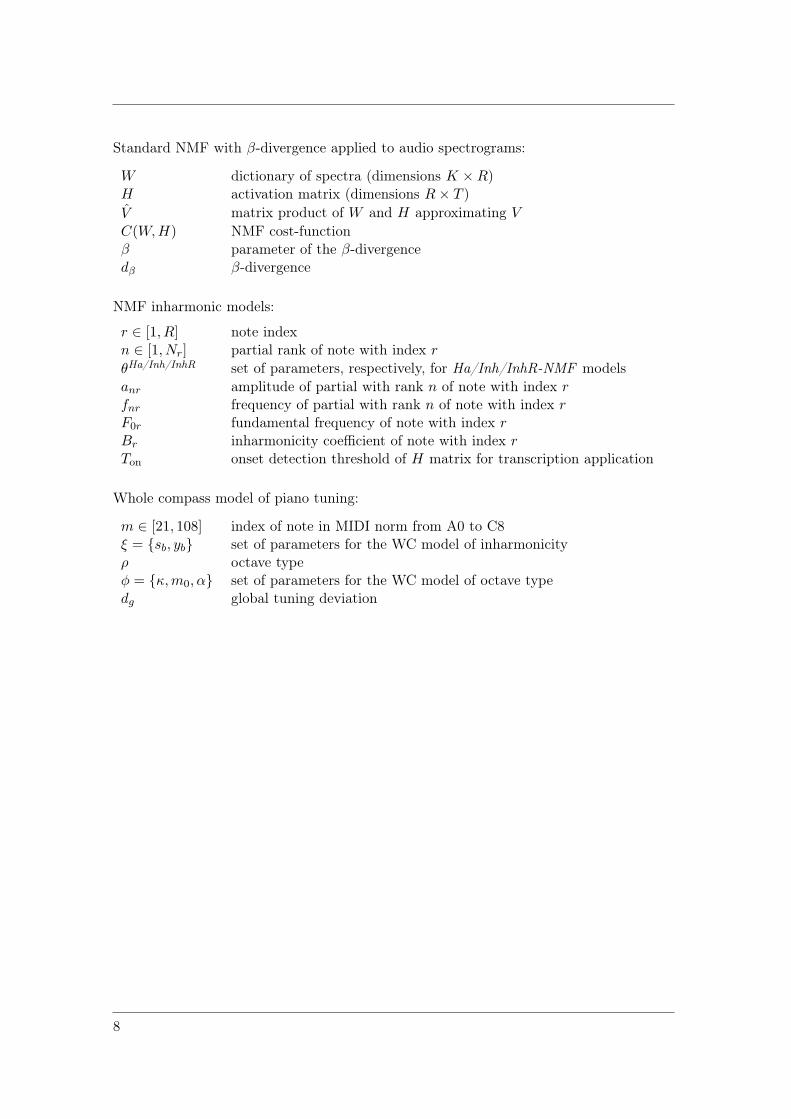
Standard NMF with β-divergence applied to audio spectrograms:
W dictionary of spectra (dimensions K ×R)H activation matrix (dimensions R× T )
V matrix product of W and H approximating V
C(W,H) NMF cost-functionβ parameter of the β-divergencedβ β-divergence
NMF inharmonic models:
r ∈ [1, R] note indexn ∈ [1, Nr] partial rank of note with index r
θHa/Inh/InhR set of parameters, respectively, for Ha/Inh/InhR-NMF models
anr amplitude of partial with rank n of note with index rfnr frequency of partial with rank n of note with index rF0r fundamental frequency of note with index rBr inharmonicity coefficient of note with index rTon onset detection threshold of H matrix for transcription application
Whole compass model of piano tuning:
m ∈ [21, 108] index of note in MIDI norm from A0 to C8ξ = sb, yb set of parameters for the WC model of inharmonicityρ octave typeφ = κ,m0, α set of parameters for the WC model of octave typedg global tuning deviation
8

Chapter 1
Introduction
1.1 Musical sound modeling and representation
Acoustics-based vs. signal-based approaches
The issue of the representation and the modeling of musical sounds is a very active re-search topic that is often addressed from two main different perspectives, namely those ofacoustics and signal processing.
Historically related to the branch of wave physics, and notably led by Helmholtz’sadvances in physical and physiological acoustics [Helmholtz, 1863], the community of in-strumental acoustics has formed around this problem by studying the mechanisms thatproduce the sound, i.e. the musical instruments. Such an approach usually relies on a pre-cise physical modeling of the vibrations and couplings taking place in musical instrumentswhen subject to a player excitation [Rossing and Fletcher, 1995; Fletcher and Rossing,1998; Chaigne and Kergomard, 2008]. For each specific instrument, the characteristics ofthe tones are related to meaningful low-level parameters such as, the physical propertiesof the materials, the geometry of each component (e.g. strings, plates, membranes, pipes),the initial conditions related to playing techniques, etc. For different designs of the sameinstrument, these modeling parameters provide a representation useful in various applica-tions. For instance, in synthesis, the control of the characteristics of the tones can be doneintuitively by modifying the physical properties of the instrument. Such representationsare also useful for psycho-acoustics research, when studying the effects of the instrumentaldesign and playing techniques on the sound and its perception.
In contrast to the physics-based approach, the community of music signal processingaims at modeling musical sounds according to their “morphological” attributes, withoutnecessarily paying due regard to the particular instruments that are played. Indeed, mostmusic signals are generally composed of tonal components (quasi-sinusoidal waves, alsocalled partials, having amplitude and frequency parameters that may vary over time),but also percussive components corresponding to attack transients, and noise. However,such kind of signal-based characteristics are hardly identifiable when having a look at awaveform representation.
Thus, a substantial part of the research in the 60’s-70’s had focused on the design oftransforms/representations that allow for an intuitive visualization and manipulation ofthese signal-based features in the time-frequency domain (as for instance the well-known
9

spectrogram based on the Short-Time Fourier Transform). Also, the inversion property ofsuch transforms led the way for analysis/synthesis applications to audio coding [Flanaganand Golden, 1966] and sound transformations (e.g. transposition, time-stretching, crosssynthesis) [Allen, 1977]. Based on these representations a number of parametric mod-els of speech/music signals have been developed, such as the sinusoidal additive model[McAulay and Quatieri, 1986; Serra and Smith, 1990] or the source-filter model (first in-troduced as a signal-model mimicking the mechanism of speech production [Fant, 1960],but further widely applied to various types of instrumental tones). In the following decade,a number of enhanced transforms have been introduced (e.g. spectral reassignment, Mod-ified Cosine Transform, Wavelet Transform, Constant Q Transform) in order to face thetime-frequency resolution trade-off or improve the coding performance by accounting forauditory perception [Mallat, 2008; Roads, 2007].
Since then, a number of theoretical frameworks, often taken from other domains suchas image processing, statistics and machine learning, have been adopted in order to replacead-hoc modelings and heuristic estimation techniques. To cite only a few, sparse coding[Mallat and Zhang, 1993; Chen et al., 1998], Bayesian modeling [Gelman et al., 2003], high-resolution methods [Badeau et al., 2006] or approaches based on rank reduction [Cichockiet al., 2009] have been widely spread across the audio community since the 90’s. In contrastwith acoustics-based modelings, these frameworks are generic enough to process complexmixture of sounds that can include various types of instruments. In parallel, a new fieldof applications, referred to as Music Information Retrieval (MIR), has emerged with aneed of indexing and classifying the ever-growing amount of multimedia data availableon the internet [Downie, 2006; Casey et al., 2008]. In this context, new kind of mid-levelrepresentations (e.g. chromagrams, onset detection functions, similarity matrices) havebeen found useful for extracting content-based information from music pieces (e.g. chords,melody, genre).
Mixing both approaches
Although acoustics and signal processing model musical tones according to different per-spectives, both communities tend to borrow tools from each other.
For instance, synthesis applications based on physical modeling require an importantnumber of parameters that cannot be easily estimated from instrument design only. In-deed, such models based on coupled differential equation systems are usually non-invertibleand a joint estimation of all parameters from a target sound is hardly practicable. Thus,the learning of the synthesis parameters often requires physical measurements on real in-struments and/or estimation techniques derived from signal-based modeling (e.g. HighResolution methods applied to modal analysis [Ege et al., 2009; Elie et al., 2013]). Also,signal processing tools such as numerical methods for differential equation solving (e.g.finite element and finite difference methods), and digital filtering are commonly used toperform the synthesis [Rauhala et al., 2007b; Bank et al., 2010].
Conversely, a general trend in signal processing this last decade (as shown in Chapter 2)tends to include prior information about the structure of the tones in order to tailor moreefficient models and estimation algorithms. For instance, accounting for the harmonicstructure of sustained tones, the smoothness of their spectral and temporal envelopes,can outperform generic models in various applications such as transcription or sourceseparation.
10

CHAPTER 1. INTRODUCTION
1.2 Approach and issues of the thesis
General framework of the thesis
The goal of this thesis is to go a step further in the mixing of both approaches. Fromgeneric signal-based frameworks we aim at including information about the timbre of thetones in order to perform analysis tasks that are specific to a given instrument. Issuesrelated to both acoustics and signal processing applications are then investigated:
• Can such classes of models be used to efficiently learn physics-related parameters(e.g. information about the design and tuning) of a specific instrument?
• Does refining/complexifying generic signal models actually improve the performanceof analysis tasks targeted by the MIR community?
It however remains unrealistic to try to combine full synthesis models, built fromacoustics only, into complex signal-based analysis methods, and to optimize both types ofparameters. Instead, we here focus on a selection of a few timbre features that should bemost relevant. This relates to one of the core concepts of musical acoustics – but also oneof the hardest to apprehend: timbre. The simplest, and standard definition of timbre1,is what differentiates two tones with the same pitch, loudness, and duration. However,timbre is much more complex than this for instrument makers, as one instrument mustbe built and tuned in such a way that its timbre keeps a definite consistency from note tonote (while not being exactly the same) across the whole tessitura, loudness and playingtechniques.
Focus on piano music
Such methodology is applied in this thesis to the case of the piano. Its study is particularlyrelevant as it has been central to Western music in the last two centuries, with an extremelywide solo and orchestral repertoire. Moreover, the analysis of piano music represents achallenging problem because of the versatility of the tones. Indeed, the piano register spansmore than seven octaves, with fundamental frequencies ranging approximately from 27 Hzto 4200 Hz, and the action mechanism allows for a wide range of dynamics. In addition,the tones are well known for their property of inharmonicity (the partial frequencies areslightly higher than those of a harmonic comb) that has an important influence in theperception of the instrument’s timbre as well as on its tuning [Martin and Ward, 1961].Thus, in this thesis particular attention is paid to the inclusion of the inharmonicity insignal-based models. Variability of the inharmonicity along the whole compass of thepiano and its influence on the tuning are also investigated.
Signal-based frameworks
This thesis focuses on Non-negative Matrix Factorization (NMF) models [Lee and Seung,1999]. Such models essentially target the decomposition of time-frequency representa-tions of music signals into two non-negative matrices: one dictionary containing the spec-tra/atoms of the notes/instruments, and one activation matrix containing their temporal
1“attribute of sensation in terms of which a listener can judge that two sounds having the same loudnessand pitch are dissimilar”, American Standards Association definition 12.9
11

activations. Thus a substantial part of this thesis consists of finding a way of enforc-ing the inharmonic structure of the spectra of the dictionary for applications related toboth acoustics (estimation of the inharmonicity parameters) and signal processing (tran-scription). An alternative model based on a Bayesian framework is also proposed in thisthesis.
1.3 Overview of the thesis and contributions
Chapter 2 - State of the art: This chapter introduces the theoretical backgroundof this thesis. First, a state-of-the-art on the Non-Negative Matrix (NMF) factorizationframework is presented. Both standard and constrained approaches are detailed, andpractical considerations about the problem formulation and the optimization are discussed.Second, basic notions of piano acoustics are presented in order to highlight some propertiesof the tones that should be relevant to include in our models. Then, a state of the art onmethods taking into account inharmonicity for piano music analysis is presented. Finally,issues resulting from the inharmonicity inclusion in signal-based models are discussed.
Chapter 3 - Estimating the inharmonicity coefficient and the F0 of piano tones:This chapter deals with the estimation of the inharmonicity coefficient and the F0 of pianotones along the whole compass, in both monophonic and polyphonic contexts.
Contributions: Two new frameworks in which inharmonicity is included as aparameter of signal-based models are presented. All presented methods exhibitperformances that compare favorably to a state of the art algorithm when appliedto the supervised estimation of the inharmonicity coefficient and the F0 of isolatedpiano tones.
First in Section 3.1, two NMF-based parametric models of piano tone spectrafor which different types of inclusion of the inharmonicity is proposed (strict andrelaxed constraints) are described. Estimation algorithms are derived for bothmodels and practical considerations about the initialization and the optimiza-tion scheme are discussed. These are finally applied on isolated note and chordrecordings in a supervised context (i.e. with the knowledge of the notes that areprocessed).
Second in Section 3.2, a generative probabilistic model for the frequenciesof peaks with significant energy in time-frequency representations is introduced.The parameter estimation is formulated as a maximum a posteriori problem andsolved by means of an Expectation-Maximization algorithm. The precision of theestimation of the inharmonicity coefficient and the F0 of piano tones is evaluatedfirst on isolated note recordings in both supervised and unsupervised cases. Forthe unsupervised case, the algorithm returns estimates of the inharmonicity co-efficients and the F0s as well as a probability for each note to have generated theobservations in each time-frame. The algorithm is finally applied on a polyphonicpiece of music in an unsupervised way.
Chapter 4 - A parametric model for the inharmonicity and tuning along thewhole compass: This chapter presents a study on piano tuning based on the consider-ation of inharmonicity and tuner’s influences.
12
CHAPTER 1. INTRODUCTION
Contributions: A joint model for the inharmonicity and the tuning of pianosalong the whole compass is introduced. While using a small number of parame-ters, these models are able to reflect both the specificities of instrument designand tuner practice. Several applications are then proposed. These are first usedto extract parameters highlighting some tuners’ choices on different piano typesand to propose tuning curves for out-of-tune pianos or piano synthesizers. Also,from the study on several pianos, an average model useful for the initializationof the inharmonicity coefficient and the F0 of analysis algorithms is obtained.Finally, these models are applied to the interpolation of inharmonicity and tun-ing along the whole compass of a piano, from the unsupervised analysis of apolyphonic musical piece.
Chapter 5 - Application to the transcription of polyphonic piano music: Thischapter presents an application to a transcription task of the two NMF-based algorithmsintroduced in Section 3.1.
Contributions: In order to quantify the benefits that may result from the in-harmonicity inclusion in NMF-based models, both algorithms are applied to atranscription task and compared to a simpler harmonic model. We study on a 7-piano database the influence of the model design (harmonicity vs. inharmonicityand number of partials considered), of the initialization (naive initialization vs.mean model of inharmonicity and tuning along the whole compass) and of theoptimization process. Results suggest that it is worth including inharmonicityin NMF-based transcription model, provided that the inharmonicity parametersare sufficiently well initialized.
Chapter 6 - Conclusion and prospects: This last chapter summarizes the contribu-tions of the present work and proposes some prospects for the design of a competitive pianotranscription system and the application of such approaches for other string instrumentssuch as the guitar.
1.4 Related publications
— Peer-reviewed journal article —
Rigaud, F., David, B., and Daudet, L. (2013a). A parametric model and estimationtechniques for the inharmonicity and tuning of the piano. Journal of the AcousticalSociety of America, 133(5):3107–3118.
— Peer-reviewed conference articles —Society of America, 133(5):3107–3118.
— Peer-reviewed conference articles —
Rigaud, F., David, B., and Daudet, L. (2011). A parametric model of piano tuning.In Proceedings of the 14th International Conference on Digital Audio Effects (DAFx),pages 393–399.
Rigaud, F., David, B., and Daudet, L. (2012). Piano sound analysis using non-negativematrix factorization with inharmonicity constraint. In Proceedings of the 20th EuropeanSignal Processing Conference (EUSIPCO), pages 2462–2466.
13

Rigaud, F., Drémeau, A., David, B., and Daudet, L. (2013b). A probabilistic line spectrummodel for musical instrument sounds and its application to piano tuning estimation. InProceedings of the IEEE Workshop on Applications of Signal Processing to Audio andAcoustics (WASPAA).
Rigaud, F., Falaize, A., David, B., and Daudet, L. (2013c). Does inharmonicity improvean NMF-based piano transcription model? In Proceedings of the IEEE InternationalConference on Acoustics, Speech and Signal Processing (ICASSP), pages 11–15.
14

Chapter 2
State of the art
This thesis mainly focuses on the inclusion of specific properties of the timbre of piano tonesin Non-negative Matrix Factorization (NMF) models. Thus, this chapter first presents inSection 2.1 a state-of-the-art on the modeling of audio spectrograms based on the NMFframework. Both standard and constrained formulations accounting for specific audioproperties are detailed. Then in Section 2.2, some basic notions of instrumental acousticsare introduced in order to highlight some characteristics of piano tones that should berelevant to blend into the NMF model. Finally, a state-of-art of methods including theinharmonic nature of the tones in piano music analysis is presented and issues resultingfrom its inclusion in signal models are discussed in Section 2.3.
2.1 Modeling time-frequency representations of audio signals
based-on the factorization of redundancies
Most musical signals are highly structured, both in terms of temporal and pitch arrange-ments. Indeed, when analyzing the score of a piece of western tonal music (cf. for instanceFigure 2.1) one can notice that often a restricted set of notes whose relationship are givenby the tonality are used and located at particular beats corresponding to subdivisionsof the measure. All these constraints arising from musical composition rules (themselvesbased on musical acoustics and psycho-acoustics considerations) lead to a number of re-dundancies: notes, but also patterns of notes, are often repeated along the time line.
Figure 2.1: Score excerpt of the Prelude I from The Well-Tempered Clavier Book I - J.S.Bach. Source: www.virtualsheetmusic.com/
Taking these redundancies into account to perform coding, analysis and source separa-
15

tion of music signals has become a growing field of research in the last twenty years. Orig-inally focused on speech and image coding problems, the sparse approximation frameworkaims at representing signals in the time domain as a linear combination of a few patterns(a.k.a. atoms) spanning different time-frequency regions [Mallat and Zhang, 1993; Chenet al., 1998]. The dictionary of atoms is usually highly redundant, it may be given a priorior learned from a separate dataset. It may also be structured in order to better fit thespecific properties of the data (e.g. harmonic atoms for applications to music [Gribonvaland Bacry, 2003; Leveau et al., 2008]).
In the last decade, the idea of factorizing the redundancies inherent to the structureof the music has been applied to signals in the time-frequency domain. Unlike the signalwaveform, time-frequency representations such as the spectrogram allow for an intuitiveinterpretation of the pitch and rhythmic content by exhibiting particular characteristicsof the musical tones (e.g. a comb structure evolving over time for pitched sounds, cf.Figure 2.2). Beyond the recurrence of the notes that are played (cf. note E5 whosespectro-temporal pattern is highlighted in black in Figure 2.2(b)), adjacent time-framesare also highly redundant. Thus, methods based on redundancy factorization such asthe Non-negative Matrix Factorization (NMF) [Lee and Seung, 1999], or it probabilisticcounterpart the Probabilistic Latent Component Analysis (PLCA) [Smaragdis et al., 2008]have been applied to musical signals with the goal to decompose the observations into a fewmeaningful objects: the spectra of the notes that are played and their activations over time.Another seducing property of these approaches is that the dictionary of spectra/atoms maybe directly learned from the data, jointly with the estimation of the activations. However,this great flexibility of factorization approaches often makes difficult the interpretation ofactivation patterns as individual note activation. In order to be successfully applied tocomplex tasks such as polyphonic music transcription or source separation, the structureof the decomposition has to be enforced by including prior information on the specificproperties of audio data in the model (for instance harmonic structure of sustained notespectra or smoothness of temporal activations).
2.1.1 Non-negative Matrix Factorization framework
The NMF is a decomposition method for multivariate analysis and dimensionality/rankreduction of non-negative data (i.e. composed of positive or null elements) based on thefactorization of the redundancies naturally present. Unlike other techniques such as Inde-pendent Component Analysis [Comon, 1994] or Principal Component Analysis [Hotelling,1933] for which the factorized elements may be composed of positive and negative ele-ments, the key point of NMF relies on the explicit inclusion of a non-negativity constraintthat enforces the elements of the decomposition to lie in the same space as the observa-tions. Thus, when analyzing data composed of non-negative elements, such as the pixelintensity of images, the decomposition provided by the NMF exhibits a few meaningfulelements that can be directly interpreted as distinctive parts of the initial images (forinstance the eyes or the mouth of face images [Lee and Seung, 1999]).
Although the first NMF problem seems to be addressed in [Paatero and Tapper, 1994]under the name Positive Matrix Factorization, is has been widely popularized by thestudies of Lee and Seung [Lee and Seung, 1999, 2000] which highlighted the ability of themethod for learning meaningful parts of objects (images and text) and proposed efficientalgorithms. Since then, an important number of studies have been dealing with extend-
16

CHAPTER 2. STATE OF THE ART
0 0.5 1 1.5 2 2.5 3 3.5
1
0.5
0
0.5
1
Time (s)
(a)
Time (s)
Fre
qu
en
cy (
Hz)
0.5 1 1.5 2 2.5 3 3.50
500
1000
1500
2000
2500
3000
3500
4000
4500
(b)
Figure 2.2: (a) waveform and (b) spectrogram of the first bar of the score given in Figure2.1. The spectral pattern of note E5 is highlighted in black.
ing NMF models and algorithms to applications in data analysis and source separation[Cichocki et al., 2009] in various domains such as, to name only a few, image [Lee andSeung, 1999; Hoyer, 2004], text [Lee and Seung, 1999; Pauca et al., 2004], biological data[Liu and Yuan, 2008] or audio processing [Smaragdis and Brown, 2003].
2.1.1.1 Model formulation for standard NMF
Given the observation of a non-negative matrix V of dimension K × T , the NMF aims atfinding an approximate factorization:
V ≈WH = V , (2.1)
where W and H are non-negative matrices of dimensions K ×R and R× T , respectively.Thus, the observation matrix V is approximated by a positive linear combination of Ratoms, contained in the dictionary W whose weightings are given by the coefficients of H,also called the activation matrix. For each element Vkt, Equation (2.1) leads to:
Vkt ≈R∑
r=1
WkrHrt = Vkt . (2.2)
The model is illustrated in Figure 2.3 on a toy example, where the exact factorization ofa rank-3 matrix is obtained. In real-life applications, V is usually full-rank and only anapproximate factorization can be obtained. In order to obtain a few meaningful atoms inthe dictionary W , the order of the model R is usually chosen so that KR + RT ≪ KT ,which corresponds to a reduction of the dimensionality of the data. The optimal tuning of
17

R is not straightforward. It is usually arbitrarily chosen, depending on which application istargeted. For the interested reader, more theoretical considerations and results about theoptimal choice of R and the uniqueness of NMF may be found in [Cohen and Rothblum,1993; Donoho and Stodden, 2004; Laurberg et al., 2008; Klingenberg et al., 2009; Essid,2012].
Figure 2.3: NMF illustration for an observation matrix V of rank 3. The superposition ofthe elements (squares, disks and stars) in V corresponds to a summation. In this particularexample, the activation matrix H is composed of binary coefficients.
2.1.1.2 Applications to music spectrograms
In the case of applications to audio signals, V usually corresponds to the magnitude (orpower) spectrogram of an audio excerpt, k being the frequency bin index and t being theframe index. Thus, W represents a dictionary containing the spectra of the R sources, andH their time-frame activations. Figure 2.4 illustrates the NMF of a music spectrogramin which one can see that two notes are first played separately, and then jointly. For thisparticular example, when choosing R = 2 the decomposition accurately learns a meanstationary spectrum for each note in W and returns their time-envelopes in H, even whenthe two notes are played jointly.
Figure 2.4: NMF applied to the decomposition of an audio spectrogram.
18

CHAPTER 2. STATE OF THE ART
This convenient and meaningful decomposition of audio spectrograms led the way forapplications such as automatic music transcription (the transcription task is presented inmore detail in Chapter 5) [Smaragdis and Brown, 2003; Paulus and Virtanen, 2005; Bertin,2009], audio source separation [Virtanen, 2007; Ozerov and Févotte, 2010], audio-to-scorealignment [Cont, 2006], or audio restoration [Le Roux et al., 2011].
However, it should be noticed that although the additivity of the sources1 is preservedin the time-frequency domain by the Short-Time Fourier Transform, a mixture spectro-gram is not the sum of the component spectrograms because of the non-linearity of theabsolute value operator. Thus, the NMF model, as it is given in Equation (2.1), is strictlyspeaking incorrect and some studies have introduced a modeling of the phase compo-nents [Parry and Essa, 2007a,b] in order to refine the model. However, in most casesthe validity of the standard NMF model is still justified by the fact that for most musicsignals the sources are spanning different time-frequency regions and each time-frequencybin’s magnitude is often explained by a single predominant note/instrument [Parvaix andGirin, 2011]. When several sources are equally contributing to the energy contained in atime-frequency bin, the exponent of the representation (for instance 1 for the magnitudespectrogram and 2 for the power spectrogram) may have an influence on the quality of theNMF approximation. In the case of independent sources (for instance corresponding todifferent instruments), it seems that a better approximation is obtained for an exponentequal to 1 (i.e. V is a magnitude spectrogram) [Hennequin, 2011].
Besides the factorization of spectrograms, other types of observation matrices may beprocessed when dealing with musical data. For instance, the NMF has been applied tothe decomposition of self-similarity matrices of music pieces for music structure discovery[Kaiser and Sikora, 2010], or matrices containing audio features for musical instrument[Benetos et al., 2006] and music genre [Benetos and Kotropoulos, 2008] classification.
2.1.1.3 Quantification of the approximation
In order to quantify the quality of the approximation of Equation (2.1), a measure ofthe dissimilarity between the observation and the model is evaluated by means of a dis-tance (or divergence), further denoted by D(V | WH). This measure is used to define areconstruction cost-function
C(W,H) = D(V |WH), (2.3)
from which H and W are estimated according to a minimization problem
W , H = argminW∈RK×R
+ ,H∈RR×T+
C(W,H). (2.4)
For a separable metric, the measure can be expressed as:
D(V |WH) =K∑
k=1
T∑
t=1
d(Vkt | Vkt
), (2.5)
where d(. | .) denotes a measure of dissimilarity between two scalars, corresponding forinstance to each time-frequency bin of the observed spectrogram and the model. A wide
1This holds for music signals obtained by a linear mixing of the separated tracks, thus by neglectingthe non-linear mixing operations such as for instance the compression applied at the mastering.
19
range of metrics have been investigated for NMF, often gathered in families such as theCsiszar [Cichocki et al., 2006], β [Févotte and Idier, 2011] or Bregman divergences [Dhillonand Sra, 2006]. It is worth noting that divergences are more general than distances sincethey do not necessarily respect the properties of symmetry and triangular inequality.However they are still adapted to a minimization problem since they present a singleminimum for Vkt = Vkt.
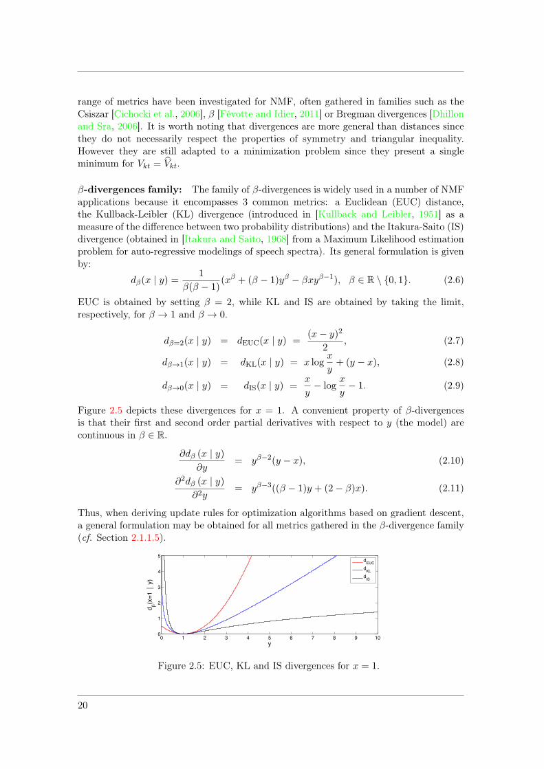
β-divergences family: The family of β-divergences is widely used in a number of NMFapplications because it encompasses 3 common metrics: a Euclidean (EUC) distance,the Kullback-Leibler (KL) divergence (introduced in [Kullback and Leibler, 1951] as ameasure of the difference between two probability distributions) and the Itakura-Saito (IS)divergence (obtained in [Itakura and Saito, 1968] from a Maximum Likelihood estimationproblem for auto-regressive modelings of speech spectra). Its general formulation is givenby:
dβ(x | y) =1
β(β − 1)(xβ + (β − 1)yβ − βxyβ−1), β ∈ R \ 0, 1. (2.6)
EUC is obtained by setting β = 2, while KL and IS are obtained by taking the limit,respectively, for β → 1 and β → 0.
dβ=2(x | y) = dEUC(x | y) =(x− y)2
2, (2.7)
dβ→1(x | y) = dKL(x | y) = x logx
y+ (y − x), (2.8)
dβ→0(x | y) = dIS(x | y) =x
y− log
x
y− 1. (2.9)
Figure 2.5 depicts these divergences for x = 1. A convenient property of β-divergencesis that their first and second order partial derivatives with respect to y (the model) arecontinuous in β ∈ R.
∂dβ (x | y)∂y
= yβ−2(y − x), (2.10)
∂2dβ (x | y)∂2y
= yβ−3((β − 1)y + (2− β)x). (2.11)
Thus, when deriving update rules for optimization algorithms based on gradient descent,a general formulation may be obtained for all metrics gathered in the β-divergence family(cf. Section 2.1.1.5).
0 1 2 3 4 5 6 7 8 9 100
1
2
3
4
5
y
d(x
=1
y)
dEUC
dKL
dIS
Figure 2.5: EUC, KL and IS divergences for x = 1.
20

CHAPTER 2. STATE OF THE ART
Scaling properties: When dealing with a specific application, the choice of thecost-function should be done according to the particular properties of the data. In thecase where the NMF is applied to the factorization of audio spectrograms, an importantconsideration to take into account is that magnitude spectra have a large dynamic range.As illustrated on Figure 2.6(a), audio spectra are usually characterized by a fast decreaseof the spectral envelope and only a few partials with low rank have a large magnitude.However, some higher-rank partials with lower magnitudes still have significant loudnessfor auditory perception, this latter being more closely related to a logarithmic scale (cf.Figure 2.6(b)). Likewise, along the time-frame axis, spectrograms contain much moreenergy at attack transients than in decay parts. Thus, an important feature to considerwhen choosing a divergence is its scaling property [Févotte et al., 2009]. When dealingwith β−divergences the following expression is obtained from Equation (2.6):
dβ(γx | γy) = γβ · dβ(x | y), γ ∈ R+. (2.12)
It implies that according to the value of β, different relative weights will be given in thecost-function (Equation (2.5)) for each time-frequency bin depending on its magnitude.For instance, for β > 0 the reconstruction of time-frequency bins presenting highest mag-nitudes will be favored since a bad fit on these coefficients will cost more than an equallybad fit on these with lowest magnitude. For β < 0 a converse effect will be obtained. Onlyβ = 0, which corresponds to the IS divergence, exhibits a scale invariance property whichshould be suitable for applications to audio source separation since it should allow for areliable reconstruction of all coefficient regardless of their magnitude, even low-valued onesthat may be audible [Févotte et al., 2009]. For these reasons, most studies related to au-dio applications usually consider values of β ∈ [0, 1] [Virtanen, 2007; Ozerov and Févotte,2010; Vincent et al., 2010; Dessein et al., 2010]. EUC is rarely used, and it is sometimesreplaced by weighted Euclidean distances using perceptual frequency-dependent weights[Vincent and Plumbey, 2007; Vincent et al., 2008]. However, a fine tuning of β within therange [0, 1] is not straightforward and seems to be dependent on the application and onthe value of the spectrogram exponent (e.g. 1 for a magnitude or 2 for a power spectro-gram). A detailed study on the β parameter has shown that a KL divergence for processingmagnitude spectrograms in source separation applications was leading to highest perfor-mances (evaluated in terms of Signal-to-Distortion Ratio (SDR), Signal-to-InterferenceRatio (SIR) and Signal-to-Artifacts Ratio (SAR)) [FitzGerald et al., 2009]. When pro-cessing power spectrograms for the same dataset, performances were found optimal forβ = 0.5, but lower than those obtained on magnitude spectrograms. In application topolyphonic transcription [Vincent et al., 2010], optimal pitch estimation performances(F-measure) were obtained for β = 0.5 when processing magnitude spectrograms.
Convexity: Another important property to ensure that the optimization problemholds a single minimum is the convexity of the cost-function. Equation (2.10) shows thatβ-divergences present a single minimum for x = y and increase with | x − y |. However,the convexity with respect to y for x fixed is limited to the range β ∈ [1, 2] (cf. Equa-tion (2.11)). Thus, IS is non-convex and present an horizontal asymptote for β → +∞.Moreover, even for β ∈ [1, 2], the convexity of β-divergences does not necessarily lead tothe convexity of the reconstruction cost-function given in Equation (2.5) since the opti-mization of the parameters Wk,rk∈[1,K],r∈[1,R] and Hr,tr∈[1,R],t∈[1,T ] should be jointly
21

0 2000 4000 6000 8000 10000 12000 14000 160000
0.2
0.4
0.6
0.8
1
Frequency (Hz)
Ma
g.
sp
ectr
um
(lin
. sca
le)
(a)
0 2000 4000 6000 8000 10000 12000 14000 16000−140
−120
−100
−80
−60
−40
−20
0
Frequency (Hz)
Ma
g.
sp
ectr
um
(lo
g.
sca
le)
(b)
Figure 2.6: Magnitude spectrum of a piano note A3 in (a) linear and (b) dB scale.
performed. Thus, most algorithms perform updates of the parameters in an iterative way,each coefficient being independently updated while others are kept fixed.
In the case where dependencies are considered for the elements of W or H, for instanceby setting parametric models (cf. Section 2.1.2.2), the convexity of the cost-function withrespect to the new highest-level parameters will not necessarily be verified and heuristicsmay be used to ensure that the algorithm does not stop in a local minimum (as shown inSection 3.1.2.2 where an NMF parametric model for piano sound analysis is introduced).
2.1.1.4 Notes about probabilistic NMF models
As seen so far, solving an NMF problem requires the choice of a cost-function, this latterbeing usually done according to a trade-off between the specific properties of the observa-tions and the convexity of the problem. An alternative method consists of considering theset of observations as a realization of a generative process composed of random variables.Thus, the choice of the probability distribution that is associated to each variable providesa cost function, for instance by considering a maximum-likelihood formulation. A mainbenefit of the probabilistic framework relies in the possibility of including informationabout the data by setting a priori distributions on the NMF parameters, and accordingto Bayesian inference solving a maximum a posteriori problem. For instance, in [Yoshiokaand Sakaue, 2012] a log-normal distribution is assumed for each element of the dictionaryof spectra Wkt. This choice leads to a cost-function corresponding to the squared errorbetween the observation and the model spectrograms with logarithmic magnitude. Sucha model can account for the high dynamic range of audio signals, as discussed above.
In some cases, both deterministic and probabilistic approaches can be shown to beequivalent [Févotte and Cemgil, 2009]. For instance, taking standard NMF cost-function(Equation (2.5)) with KL divergence is equivalent to considering that the sources, indexedby r, that contribute to the generation of a time-frequency bin of the observed magnitudespectrogram Vkt, are independent and distributed according to a Poisson distribution
22

CHAPTER 2. STATE OF THE ART
with parameter WkrHrt [Virtanen et al., 2008]. For IS an equivalence is obtained byassuming that each source independently contributes to the time-frequency bin of thepower spectrogram | Vkt |2 according to a complex Gaussian distribution with null meanand variance WkrHrt [Févotte et al., 2009].
2.1.1.5 Optimization techniques
A wide variety of continuous optimization algorithms can be used to solve problem (2.5)[Cichocki et al., 2008]. For instance, standard algorithms based on gradient descent [Lin,2007; Wang and Zou, 2008] or Newton methods [Zdunek and Cichocki, 2007] may beapplied to NMF problems. However, in order to preserve the non-negativity of the decom-position obtained with these methods a projection onto the positive orthant is requiredafter each update. Thus, other methods that implicitly preserve the non-negativity areusually preferred. Among such techniques, the most popular are very likely the multi-plicative algorithms whose update rules can be obtained from heuristic decompositions ofthe cost-function or in a more rigorous way by using Majorization-Minimization (MM)methods [Lee and Seung, 2000; Févotte and Idier, 2011]. In the case of probabilistic NMFmodels, methods such as the Expectation-Maximization algorithm [Dempster et al., 1977]or variants such as the Space-Alternating Generalized Expectation-Maximization (SAGE)algorithm [Fessler and Hero, 2010; Bertin et al., 2010] are commonly used.
Multiplicative algorithms are the most employed in practice because they guaranteethe non-negativity of the decomposition and it is often experimentally verified that theylead to satisfactory solutions with a reasonable computational time. Thus, for the NMFmodels proposed in this thesis we chose to focus on this method in order to perform theoptimizations.
Multiplicative algorithms: The heuristic approach for deriving multiplicative updatesconsists of decomposing the partial derivatives of a cost function, with respect to a givenparameter θ∗, as a difference of two positive terms:
∂C(θ∗)∂θ∗
= P (θ∗)−Q(θ∗), P (θ∗), Q(θ∗) ≥ 0 (2.13)
and at iteratively updating the corresponding parameter according to:
θ∗ ← θ∗ ×Q(θ∗)/P (θ∗) (2.14)
Since P (θ∗) and Q(θ∗) are positive, it guarantees that parameters initialized with positivevalues stay positive during the optimization, and that the update is performed in thedescent direction along the parameter axis. Indeed, if the partial derivative of the costfunction is positive (respectively negative), then Q(θ∗)/P (θ∗) is smaller (resp. bigger)than 1 and the value of the parameter is decreased (resp. increased). At a stationarypoint, the derivative of the cost function is null so Q(θ∗)/P (θ∗) = 1.
When applied to the NMF model with β-divergences, the following expressions for thegradient are obtained by using Equations (2.5) and (2.10):
∇HC(W,H) = W T((WH).[β−2] ⊗ (WH − V )
), (2.15)
∇WC(W,H) =((WH).[β−2] ⊗ (WH − V )
)HT , (2.16)
23

where ⊗ and .[] respectively denote element-wise multiplication and exponentiation, andT denotes the transpose operator. Since all matrices are composed of non-negative coeffi-cients an obvious decomposition leads to the following updates:
H ← H ⊗ W T((WH).[β−2] ⊗ V
)
W T (WH).[β−1], (2.17)
W ← W ⊗((WH).[β−2] ⊗ V
)HT
(WH).[β−1]HT, (2.18)
where the fraction bar denotes element-wise division.In the general case, no proof is given for the convergence of the algorithm or even for the
decrease of the cost-function since the decomposition (2.13) is not unique and is arbitrarilychosen. When using MM algorithms, update rules are obtained by building a majorizingfunction which is minimized in an analytic way in a second step, thus proving the decreaseof the criterion. In the case of NMF with β-divergences, identical rules to (2.17) and (2.18)have been obtained for β ∈ [1, 2] with a proof of the decrease of the criterion by using MMalgorithm formalism [Kompass, 2007]. However it should be noticed that the property ofthe decrease of the criterion does not ensure that the algorithm will end in a local and evenless in the global minimum. Moreover, it can be observed in some case that an increaseof the criterion at some iterations may lead to a much faster convergence toward a localminimum [Badeau et al., 2010; Hennequin, 2011].
2.1.2 Giving structure to the NMF
Besides the generic “blind” approach, prior information is often considered in order tobetter fit the decomposition to specific properties of the data. Indeed, the standard NMFproblem, as it is given by Equation (2.4), does not guarantee that the optimal solution issuitable regarding the targeted application. For instance, in a music transcription task itcannot be ensured that each column of W will contain the spectrum of a unique note thathas been played and not a combination of several notes. Moreover, there is no guaranteethat an optimal solution (with respect to a given application) is obtained since differentlocal optima may be reached by the algorithm, depending on the initialization of theparameters.
Thus, taking into account prior information in the initialization is a matter of impor-tance since it should help in avoiding the convergence toward minima that may not beoptimal for the considered application. For instance, since most instrumental tones sharean harmonic structure, initializing W with harmonic combs having different fundamentalfrequencies is valuable when targeting polyphonic music source separation [Fritsch andPlumbey, 2013]. Likewise, for drum separation applications, the initialization of the acti-vations of H by an onset detection function combined with a dictionary W for which thedrum sources span different frequency bands allows the recovery of the different elements(bass-drum, snare, ...) in an efficient way [Liutkus et al., 2011].
Moreover, in order to reduce the search space to meaningful solutions, such informa-tion is often also included during the optimization process. For instance, when additionaldata is available (e.g. the score of the piece of music or isolated note recordings of thesame instruments with pitch labels), one can directly use the supplementary informationto perform the decomposition in a supervised way. When it is not the case, the data prop-erties can be explicitly included in the modeling in order to constrain the decomposition in
24

CHAPTER 2. STATE OF THE ART
a semi-supervised way. In the case of audio, these can be for instance physics-based (prop-erties about the timbre of the tones), signal-based (e.g. sparsity of notes simultaneouslyplayed, smoothness of activations and temporal envelopes) or derived from musicologicalconsiderations (e.g. the note activation should be synchronized on the beat, or chordtransitions may have different probabilities depending on the tonality). For each methodpresented in the following, the inclusion of a specific property is highlighted but it shouldbe emphasized that models usually combine different types of information.
2.1.2.1 Supervised NMF
Supervised NMF methods usually consist in initializing some parameters of the decompo-sition according to some information already available, for instance provided as additionaldata, or obtained by some preliminary analysis process. These parameters are then fixedduring the optimization.
For instance, if the score of a piece of music is known, elements of the activationmatrix H are forced to 0 where is it is known that a note is not present and initialized to1 otherwise. Such approaches may be used in audio source separation [Hennequin et al.,2011b; Ewert and Müller, 2012] where thus the problem is to estimate the remainingparameters (H for non-zero coefficients and W ).
In the case where a training set is available, the dictionary of spectra W may belearned in a first step. For instance in a music transcription task, for which isolated noterecordings of the same instrument and with the same recording conditions are available, thespectra can be learned independently for each note by applying a rank-one decomposition[Niedermayer, 2008; Dessein et al., 2010]. Then, the supervised NMF problem reducesto the estimation of the activation matrix H for the considered piece of music. Similarapproaches have been applied to speech enhancement and speech recognition [Wilson et al.,2008; Raj et al., 2010].
2.1.2.2 Semi-supervised NMF
If no additional data is available, the information about the properties of the data may beexplicitly considered in the optimization (cf. Paragraph Regularization) or in the modeling(cf. Paragraph Parameterization).
Regularization: As commonly done with ill-posed problems, the NMF can be con-strained by considering a regularized problem. In practice, it consists of adding to thereconstruction cost-function some penalty terms that emphasize specific properties of thevariables. When the constraints are considered independently for W and H, which isusually the case, the optimization problem can be expressed as the minimization of a newcost-function given by:
C(W,H) = D(V |WH) + λH · CH(H) + λW · CW (W ). (2.19)
where CH(H) and CW (W ) correspond to penalty terms respectively constraining H and Wmatrices and whose weightings are given by λH and λW . The choice of the regularizationparameters λH and λW can be done using empirical rules, or through cross-validation. Inthe probabilistic NMF framework, this type of constraint is equivalent to adding a prioridistributions on H and W , as −D(V | WH) corresponds to the log-likelihood, up to aconstant.
25

A number of penalties have been proposed in the literature, for instance in order toenforce sparsity of H, i.e. reducing the set of notes that should be activated [Eggert andKörner, 2004; Hoyer, 2004; Virtanen, 2007; Joder et al., 2013], smoothness of the linesof H in order to avoid well-localized spurious activations [Virtanen, 2007; Bertin et al.,2009], or the decorrelation of the lines of H [Zhang and Fang, 2007].
Parameterization: Unlike regularization techniques that introduce the constraint in a“soft” way by favoring some particular solutions during the optimization, another commonmethod to impose structure on the decomposition is to use parametric models for thematrices W and H.
A common example is a parametrization of the dictionary W to fit to the structureof the spectra. Here, the number of parameters reduces from K × T to a few meaningfulparameters corresponding for instance to magnitudes and frequencies of the partials. In[Hennequin et al., 2010; Ewert et al., 2013] the spectra are modeled by harmonic combs,parameterized by F0 and the partials’ magnitude. In [Bertin et al., 2010] each spectrumis modeled as a linear combination of narrow-band sub-spectra, each one being composedof a few partials with fixed magnitude and all sharing a single parameter F0. This lattermodel of additive sub-spectra brings smoothness to the spectral envelope, which reducesthe activation of spurious harmonically-related notes (octave or fifth relations, for instance,where partials fully overlap) [Klapuri, 2001; Virtanen and Klapuri, 2002].
For the matrix H, the temporal regularity underlying the occurrences of note onsetsis modeled in [Ochiai et al., 2012]. Thus, each line of H is composed of smooth patternslocated around multiples or fractions of the beat period. Besides avoiding spurious acti-vations, this parametrization also makes post-processing of H easier in order to performtranscription.
Several studies also exploit in NMF the non-stationarity of musical sounds. For in-stance in [Durrieu et al., 2010, 2011] a source-filter model for main melody extractionis presented. The main melody is here decomposed in two layers, one standard-NMF(the source) where the dictionary of spectra is fixed with harmonic combs, multiplied by asecond NMF (the filter) adjusting the time-variations of the spectral envelopes with a com-bination of narrow-band filters contained in the second dictionary. In [Hennequin et al.,2011a], the temporal variations of the spectral envelopes are handled by means of a time-frequency dependent activation matrix Hrt(f) based on an auto-regressive model. Thevibrato effect is also modeled in [Hennequin et al., 2010] by considering time-dependentF0s for the dictionary of spectra. In a more flexible framework, all these temporal varia-tions (e.g. changes in the spectral content of notes between attack to decay transitions,spectral envelope variations or vibrato) are taken into account by considering several ba-sis spectra for each note/source of the dictionary and Markov-chain dependencies betweentheir activations [Nakano et al., 2010; Mysore et al., 2010].
Such methods for enforcing the structure of the NMF will inspire the models presentedin Chapters 3 and 5 of this thesis, where we focus on specific properties of the piano.
26

CHAPTER 2. STATE OF THE ART
2.2 Considering the specific properties of piano tones
This section introduces a few basic notions from musical acoustics in order to point outsome particular features of piano tones that should be relevant for piano music analysis.Thus, it is not intended to give a complete description and modeling of the instrument’selements and their interaction. We rather focus on the core element of the piano, namelythe strings, whose properties are mainly responsible for the inharmonic nature of the tones.A more detailed study about the influence of the inharmonicity in the string design andtuning is proposed in Chapter 4.
2.2.1 Presentation of the instrument
From the keyboard, which allows the player to control the pitch and the dynamics of thetones, to the propagation of the sound through the air, the production of a piano noteresults from the interaction of various excitation and vibrating elements (cf. Figure 2.7).When a key is depressed, an action mechanism is activated with a purpose to translatethe depression into a rapid motion of a hammer, this latter inducing a free vibration ofthe strings after the stroke. Because of their small radiating surface, the strings cannotefficiently radiate the sound. It is the coupling at the bridge that allows the transmissionof the vibration from the strings to the soundboard, this latter acting as a resonator andproducing an effective acoustic radiation of the sound. In order to produce tones having,as much as possible, a homogeneous loudness along the whole compass, the notes in thetreble-medium, bass and low-bass register are respectively composed of 3, 2 and 1 strings.Finally, at the release of the key, the vibration of the strings is muted by the fall of adamper.
In addition to the keyboard, pianos usually include a pedal mechanism that allows theinstrumentalist to increase the expressiveness of his playing by controlling the durationand the loudness of the notes. The most commonly used is the sostenudo pedal, that raisesthe dampers off the played strings so they keep vibrating after the key has been released.In a similar way, the damper pedal activation leads to a raise of all the piano dampers,increasing the sustain of the played notes and allowing for the sympathetic resonancesof other strings. In order to control the loudness and the color of the sound, the unacorda pedal, when activated, provokes a shift of the action mechanism so that the ham-mer strikes only two strings over the three composing the notes in the medium-treble range.
The realistic synthesis of piano tones by physical modeling requires a precise descriptionof the different elements and their interactions. Thus, a number of works have focusedon modeling specific parts and characteristics of the piano such as, the action mechanism[Hayashi et al., 1999; Hirschkorn et al., 2006], the hammer-string interaction [Suzuki,1986a; Chaigne and Askenfelt, 1993; Stulov, 1995], the pedals [Lehtonen et al., 2007], thephenomenon of sympathetic resonance [Le Carrou et al., 2005], the vibration of the strings[Young, 1952; Fletcher, 1964; Fletcher and Rossing, 1998], their coupling [Weinreich, 1977;Gough, 1981], the soundboard vibrations [Suzuki, 1986b; Mamou-Mani et al., 2008; Ege,2009]... In order to perform the synthesis, a discretization of the obtained differentialequations is usually required [Bensa, 2003; Bensa et al., 2003; Bank et al., 2010; Chabassier,2012] and the synthesis parameters are often directly obtained from measurements onpianos. Thus, the inversion of such models is usually not straightforward. For the goal ofour work, which targets the inclusion of information from physics in signal-based analysis
27

Figure 2.7: Design of grand pianos.Sources: (a) www.pianotreasure.com, (b) www.bechstein.de
models, we only focus on the transverse vibrations of the strings. This simple modelexplains, to a great extent, the spectral content of piano tones and their inharmonicproperty.
2.2.2 Model for the transverse vibrations of the strings
• Flexible strings: First consider a string characterized by its length L and linear massµ, being subject to a homogeneous tension T and no damping effects. At rest position, thestring is aligned according to the axis (Ox). When excited, its transverse displacementover time t, y(x, t) follows, at first order, d’Alembert’s differential equation:
∂2y
∂2x− µ
T
∂2y
∂2t= 0. (2.20)
By considering fixed end-point boundary conditions, the solutions correspond to station-ary waves with frequencies related by an harmonic relation fn = nF0, n ∈ N
⋆, whosefundamental frequency is given by:
F0 =1
2L
√T
µ. (2.21)
• Bending stiffness consideration: This latter model for the transverse vibration isnot precise enough to accurately describe the actual behavior of piano strings. Becauseof the important size of the strings and the properties of the piano wire (when comparedto other string instruments such as the guitar), the bending stiffness effect has to beconsidered. Then, by introducing the diameter d of the plain string, having a Young’smodulus E and an area moment of inertia I = πd4
64 , the following differential equation isobtained:
∂2y
∂2x− µ
T
∂2y
∂2t− EI
T
∂4y
∂4x= 0 (2.22)
28

CHAPTER 2. STATE OF THE ART
0 2 4 6 8 10 12 14 16 18fn / F
0
harmonic comb inharmonic comb (B=10 3
)
14
13
Figure 2.8: Comparison of an harmonic and inharmonic comb spectrum for B = 10−3.
The presence of the fourth order differential term reflects the fact that the piano wire isa dispersive medium, i.e. the vibrating modes have different propagation speed. By stillconsidering a fixed end-point boundary condition the modal frequencies can be expressedas an inharmonic relation [Morse, 1948; Fletcher and Rossing, 1998]:
fn = nF0
√1 +Bn2, n ∈ N
⋆, (2.23)
where
B =π3Ed4
64TL2(2.24)
is a dimensionless coefficient called the inharmonicity coefficient. Since the mechanicalcharacteristics of the strings differ from one note to another, obviously F0 but also B arevarying along the compass (typical values for B are in the range 10−5-10−2, from the low-bass to the high-treble register [Young, 1952; Fletcher, 1964]). Perceptual studies haveshown that inharmonicity is an important feature of the timbre of piano tones [Fletcheret al., 1962; Blackham, 1965] that should be taken into account in synthesis applications,especially for the bass range [Järveläinen et al., 2001]. In addition, it has a strong influenceon the the design [Conklin, Jr., 1996b] and on the tuning [Martin and Ward, 1961; Lattard,1993] of the instrument. This latter point is presented in more detail in Chapter 4.
In the spectrum of a note, inharmonicity results in a sharp deviation of the partialfrequencies when compared to a harmonic spectrum, and the higher the rank of the partial,the sharper the deviation. Because the inharmonicity coefficient values are quite low, thedeviation is hardly discernible for low rank partials. However, for high rank partials,the deviation becomes important and the inharmonicity consideration must be taken intoaccount when targeting spectral modeling in piano music analysis tasks. For instance, the13th partial of an inharmonic spectrum will be sharper than the 14th partial of a harmonicspectrum when considering an inharmonicity coefficient value B = 10−3 (cf. Figure 2.8).
2.2.3 Notes about the couplings
• Influence of the soundboard mobility: The modal frequencies of transverse vi-brations given by Equation (2.23) are obtained by assuming a string fixed at end-points.In practice, this consideration is a good approximation for the fixation at the pin, but itdoes not reflect the behavior of the string-soundboard coupling at the bridge. Indeed, sucha boundary condition considers a null mobility at the bridge fixation, while the actual aimof this coupling is to transfer the vibration of the string to the soundboard.
29

As well as the strings, the soundboard possesses its own vibrating modes [Conklin,Jr., 1996a; Suzuki, 1986b; Giordano, 1998; Mamou-Mani et al., 2008; Ege, 2009] and theircoupling may induce changes in the vibratory behavior of the assembly. This can be seenon Figure 2.9, where measurements of a soundboard’s transverse mobility (ratio velocityover force as a function of the frequency) are depicted in black and red, respectively, for aconfiguration “strings and plate removed” and “whole piano assembled and tuned”. Whenconsidering only the soundboard (black lines), a few well-marked modes are usually presentin the low-frequency domain (approximately under 200 Hz). While going up along thefrequency axis the modal density increases, and because of the overlap of the modes theresonances become less and less pronounced, until reaching a quasi-flat response for thehigh-frequency domain (above 3.2 kHz, not depicted here). When assembling the stringsand the soundboard, the vibratory behavior of each element is altered (cf. red curvefor the soundboard). Thus, the modal frequencies of transverse vibrations of the stringsgiven by Equation (2.23) are slightly modified. This can be observed in the spectrum ofa note, as depicted in Figure 2.10, where the partial frequencies and ranks correspondingto transverse vibrations of the strings have been picked up and represented in the graphicf2n/n
2 as a function of n2. When comparing the data to the inharmonic relation (2.23)(corresponding to a straight line in this graphic) one can notice slight deviations, mainlyfor low rank partials having frequencies for which the soundboard should present a strongmodal character.
(a) 0-200 Hz (b) 0 - 3.2 kHz
Figure 2.9: Bridge mobility (direction normal to the soundboard) of a grand piano at theendpoint of the E2 strings, after [Conklin, Jr., 1996a]. Solid black and dashed red curvesrespectively correspond to “strings and plate removed” and “piano assembled and tuned”configurations.
• Other string deformations and their coupling: Beyond the one-dimensionaltransverse deformations considered in Section 2.2.2, the propagation of several waves occurin the string after the strike of the hammer, these being able to contribute to the distincttimbre of the instrument. For instance, the propagation of longitudinal waves has beenshown to be significant for the perception, for notes in the bass range, up to A3 [Bankand Lehtonen, 2010]. For slight deformations, produced for instance when the notes areplayed with piano dynamics, the couplings between those different waves (e.g. the twopolarizations of the transverse waves, the longitudinal and the torsional waves) are neg-
30

CHAPTER 2. STATE OF THE ART
0 200 400 600 800 1000 1200 1400−60
−40
−20
0
20
40
60
Frequency (Hz)
Mag.
spectr
um
(dB
)
spectrum
partials of transverse vibration
(a)
0 50 100 150 200 250 3005950
6000
6050
6100
6150
6200
6250
n2
(fn/n
)2
data (partial frequencies and ranks)
linear regression
(b)
Figure 2.10: Influence of the string-soundboard coupling for a note E2. (a) Magnitudespectrum from which the partials corresponding to transverse vibrations of the strings areemphasized with ‘+’ markers. (b) Partial frequencies depicted in the graphic f2
n/n2 as a
function of n2 (‘+’ markers) and linear regression corresponding to the theoretical relation(2.23).
ligible and each deformation can be considered independently. Thus, when studying thepropagation of longitudinal vibration in the strings, a simple harmonic model is obtainedfor the modal frequencies [Valette and Cuesta, 1993].
In practice, for an accurate modeling of the vibratory behavior of the strings for alldynamics, all these deformations should be jointly considered, this leading to a non-linear differential equation system and explaining the apparition of the so-called “phantompartial” in the spectrum of piano tones [Conklin, Jr., 1999; Bank and Sujbert, 2005].Moreover, for notes in the medium and treble register, one should take into account thecoupling of doublets or triplets of strings (usually slightly detuned in order to increase thesustain of the sound) through the bridge [Weinreich, 1977; Gough, 1981] in order to modelthe presence of multiple partials (cf. Figure 2.11) and the double decays and beats in thetemporal evolution of partials [Aramaki et al., 2001] (cf. Figure 2.12).
31

2900 2950 3000 3050 3100
−60
−40
−20
0
20
40
Frequency (Hz)
Mag. spectr
um
(dB
)
Figure 2.11: Zoom along the frequency axis of the spectrum of a note G6 composedof a triplet of strings. Multiple peaks are present while the simple model of transversevibration for a single string assumes a single partial.
(a)
(b)
Figure 2.12: Double decay and beating of notes composed of multiple strings. Temporalevolution (a) in linear and (b) in dB, of the first 9 partials of transverse vibration for anote G♯4 played with mezzo-forte dynamics.
32

CHAPTER 2. STATE OF THE ART
2.3 Analysis of piano music with inharmonicity considera-
tion
Beyond applications related to music synthesis, the estimation of the inharmonicity coef-ficient of piano tones is an issue of importance in a number of analysis tasks such as F0
and multiple F0 estimation [Emiya et al., 2007b,a; Rauhala and Välimäki, 2007; Blanco-Martín et al., 2008], polyphonic music transcription [Emiya et al., 2010a; Benetos andDixon, 2011], temperament and tuning estimation [Lattard, 1993; Dixon et al., 2012] or pi-ano chord recognition [Ortiz-Berenguer et al., 2004; Ortiz-Berenguer and Casajús-Quirós,2002].
The methods proposed in the literature can be classified according to two main typesof approaches, the first one considers the estimation of (B,F0) from the search of thepartials related to transverse vibrations of the strings in spectra, while the second oneconsiders them as particular parameters of a signal model.
2.3.1 Iterative peak-picking and refinement of the inharmonicity coef-
ficient
This first type of method is usually based on a two-step iterative scheme that requiresthe knowledge of the notes that are being played. From rough initial values of (B,F0)(F0 being usually initialized according to Equal Temperament - cf. Appendix A - and Bbeing set to a low value, typically in the range 10−5− 10−4) a few partials located aroundthe theoretical frequencies (given by the Equation (2.23)) are selected in the magnitudespectrum in a peak-picking step. Having the frequencies and ranks of these partials,(B,F0) are refined according to the inharmonicity relation or alternative forms of it, andthe search for partials with higher ranks is iterated. Then, the procedure is usually rununtil no peak is found above a threshold on the magnitude of the spectrum. Note thatin order to increase the precision of the estimation, most methods introduce a step ofrefinement of the partial frequencies after the peak-picking, this latter being often basedon a local interpolation of the peak’s magnitude. Finally, the core difference for all thesemethods relies in the choice of the estimator that is used to compute (B,F0) from theknowledge of the partial frequencies.
For instance, in [Rauhala et al., 2007a; Rauhala and Välimäki, 2007], the PFD (PartialFrequency Deviation) algorithm estimates (B,F0) by minimizing the deviation betweenthe theoretical partial frequencies of the model and the frequencies of the peaks selectedin the magnitude spectra.
In [Emiya, 2008] an alternative form of the inharmonicity relation is proposed
f2n
n2= F 2
0 + F 20B · n2. (2.25)
and (B,F0) are estimated by means of a least-square linear regression in the plane f2n/n
2
as a function of n2.Another alternative approach estimates B by considering pairs of partials. Indeed,
in order to estimate B from the frequencies of a couple of partials (fj , fk) the followingexpression can be obtained when inverting Equation (2.23):
Bjk =j2f2
k − k2f2j
k4f2j − j4f2
k
. (2.26)
33

In practice, B cannot be robustly estimated by the simple consideration of two partialssince this estimator is highly sensitive to the frequency deviations produced by the bridgecoupling [Ortiz-Berenguer et al., 2004] . Thus, it has been proposed in [Hodgkinson et al.,2009] to estimate B by considering the median over the set of Bjk values computed foreach possible pair of partials. Such an estimator has been applied to the unsupervisedestimation of inharmonicity and temperament, together with a transcription task in apolyphonic recording context [Dixon et al., 2012].
2.3.2 Inharmonicity inclusion in signal models
The second approach consists in explicitly including (B,F0) as parameters of a signalmodel and is often used when targeting tasks such as multiple-F0 estimation or polyphonictranscription.
In [Godsill and Davy, 2005], a Bayesian framework for modeling inharmonic tones inthe time domain is introduced. (B,F0), as well as the partial amplitudes, are consideredas random variables and estimated by solving a maximum a posteriori problem. In [Davyet al., 2006], the model is extended to inharmonic tones that do not necessarily follow theinharmonicity relation given in Equation (2.23). In the time-frequency domain, a modelbased on the NMF framework has been proposed in [Vincent et al., 2008] to deal with atranscription task. (B,F0) are here included as parameters of the dictionary of spectraand optimized by minimizing a reconstruction cost-function based on a weighted Euclideannorm. Surprisingly, the transcription results were found slightly below those obtained bya simpler harmonic model. The same conclusion was found for a similar parametric NMFmodel [Hennequin, 2011], where the difficulty of updating B was encountered. Such NMF-based models will form the basis of the work presented in Chapter 3, where we investigatehow we can go beyond these limitations.
In order to avoid these difficulties in the optimization, other methods split the esti-mation problem into two sub-problems. First, they estimate (B,F0) parameters of thesignal model by optimizing a detection function designed so that the influence of the in-harmonicity parameters is put forward. Then, they estimate the remaining parameters ofthe model according to the original problem formulation. As proposed by the followingstudies, the optimization of the detection function is usually performed by means of a gridsearch over (B,F0) parameters for each possible note. Such an optimization techniquemay be found in [Galembo and Askenfelt, 1999], where they estimate the inharmonicityof piano tones by performing an inharmonic comb filtering of the magnitude spectrum.In the case of a transcription tasks, a similar approach based on an inharmonic spectralproduct has been introduced in [Emiya et al., 2010a]. This latter is applied in a firststep in order to obtain a selection of note candidates, jointly with the estimation of theirparameters (B,F0), before the estimation of the amplitude and noise parameters of themodel according to a maximum likelihood problem. A similar detection function (referredas pitch salience function) for log-frequency spectrum has been proposed in [Benetos andDixon, 2011].
2.3.3 Issues for the thesis
As seen in this section, considering the inharmonicity of piano tones in signal models doesnot seem straightforward, particularly because of optimization issues. Some works bypassthese difficulties by separating the estimation problems of (B,F0) and amplitude/noise
34

CHAPTER 2. STATE OF THE ART
parameters, but in most studies a simpler harmonic model is considered [Monti and San-dler, 2002; Marolt, 2004; Kobzantsev et al., 2005; Bello et al., 2008; Vincent et al., 2010].
The main goal of this thesis is thus to have a better understanding about the issuesarising from the inharmonicity inclusion in signal models and to investigate whether itis really valuable when targeting tasks such as polyphonic music transcription. For this,different models in which (B,F0) are included as parameters (two NMF-based models anda generative probabilistic model for the frequencies having significant energy in spectro-grams) and their optimization algorithms are introduced in Chapter 3. These are appliedto the precise estimation of (B,F0) from monophonic and polyphonic recording in bothsupervised and unsupervised conditions. A special care is taken in the initialization ofthese parameters, by introducing in Chapter 4 a model for the inharmonicity and tuningalong the whole compass of pianos. Based on invariants in design and tuning rules, themodel is able to explain the variations of piano tuning along the compass with only a fewparameters. Beyond the initialization of the analysis algorithms, it is applied to model thetuning of well-tuned pianos, to provide tuning curves for out-of-tune pianos or physically-based synthesizers and finally to interpolate the inharmonicity and tuning of pianos alongthe whole compass from the analysis of a polyphonic recording containing only a few notes.Finally the efficiency of an inharmonic model for NMF-based transcription is investigatedin Chapter 5.
35

36

Chapter 3
Estimating the inharmonicitycoefficient and the F0 of piano tones
This chapter presents two new frameworks for the estimation of (B,F0). In Section 3.1, twodifferent NMF-based models in which (B,F0) are included as parameters are presented.For each, update rules are derived and practical solutions concerning the optimization areproposed in order to avoid the convergence of the algorithms toward local minima. Bothmodels are applied to the supervised estimation (i.e. the notes are known) of (B,F0)from isolated note and chord recordings, and the performances are compared to the PFDalgorithm (described in Section 2.3). Portions of this work have been published in [Rigaudet al., 2012, 2013a]. In Section 3.2, a generative probabilistic model for the frequenciesof significant energy in the time-frequency domain is introduced. From a prior peak-picking in a magnitude spectrum, the estimation of (B,F0) is performed jointly with aclassification of each observed frequency into noise or partial components for each note ofthe model. The algorithm is then applied to the unsupervised estimation of (B,F0) fromisolated note and polyphonic recordings. This latter work has been published in [Rigaudet al., 2013b].
3.1 NMF-based modelings
The purpose of this section is to introduce the information of the inharmonicity of pianotones explicitly into the dictionary of spectra W of NMF-based modelings. The idea isto take into account the parameters (B,F0) as constraints on the partial frequencies ofeach note, so as to perform a joint estimation. In order to limit the number of parametersthat we need to retrieve, besides the amplitude and frequency of each partial, we makethe assumption that for every recording we know which notes are being played, and thecorresponding time activations. We refer to this case as supervised estimation. Then,short-time spectra are extracted from the recordings and concatenated to build the ob-servation matrix V (it is therefore not strictly speaking a spectrogram). Because for eachcolumn of V the played notes are known, the elements of H are fixed to one whenever anote is played, and zero when it is not. Thereby, only the dictionary W is optimized on thedata. In that case, we should notice that the proposed model is not a proper factorization,because there is no explicit modeling along the time axis. However, since the model isdeveloped in the NMF framework, further inclusion in transcription (cf. Chapter 5) orsource separation algorithms may still be considered, where the activations are not known
37

and must be jointly optimized (unsupervised case).
3.1.1 Modeling piano sounds in W
The model for the spectra/atoms of the dictionary W is based on an additive model:the spectrum of a note is composed of a sum of partials, in which the frequencies areconstrained by the inharmonicity relation introduced in Equation (2.23). Two differentways of enforcing the constraint are proposed. The first model (later called Inh-NMF )forces the partial frequencies to strictly comply with the theoretical inharmonicity relation,while the second model (later called InhR-NMF ) relaxes this constraint, and enhancesinharmonicity through a weighted penalty term.
3.1.1.1 General additive model for the spectrum of a note
The general parametric atom used in this work is based on the additive model proposedin [Hennequin et al., 2010]. Each spectrum of a note, indexed by r ∈ [1, R], is composedof the sum of Nr partials. The partial rank is denoted by n ∈ [1, Nr]. Each partial isparametrized by its amplitude anr and its frequency fnr. Thus, the set of parameters fora single atom is denoted by θr = anr, fnr | n ∈ [1, Nr] and the set of parameters forthe dictionary is denoted by θ = θr | r ∈ [1, R]. Finally, the expression of a parametricatom is given by:
W θrkr =
Nr∑
n=1
anr · gτ (fk − fnr), (3.1)
where fk is the frequency of the bin with index k, and gτ (fk) is the magnitude of theFourier Transform of the τ -length analysis window. In order to limit the computationaltime and to obtain simple optimization rules, the spectral support of gτ is restricted toits main lobe. For the experiments proposed in this thesis, a Hann window is used tocompute the spectra. The magnitude spectrum of its main lobe (normalized to a maximalmagnitude of 1) is given by:
gτ (fk) =1
πτ.sin(πfkτ)
fk − τ2f3k
, fk ∈ [−2/τ, 2/τ ]. (3.2)
In order to estimate the parameters, the reconstruction cost-function to minimize ischosen as the β-divergence between the observed spectra V and the model V = W θH:
C0(θ,H) =∑
k∈K
T∑
t=1
dβ
(Vkt |
R∑
r=1
W θrkr ·Hrt
). (3.3)
It is worth noting that since the partials of the model are defined on a limited set offrequency-bins fk ∈ fnr + [−2/τ, 2/τ ], the sum over k of Equation (3.3) is applied on theset K = k | fk ∈ fnr + [−2/τ, 2/τ ], ∀n ∈ [1, Nr], ∀r ∈ [1, R].
3.1.1.2 Inharmonic constraints on partial frequencies
• Strictly inharmonic / Inh-NMF:
38

CHAPTER 3. ESTIMATING THE INHARMONICITY COEFFICIENT AND THE F0 OF PIANO TONES
The strict inharmonic constraint consists in fixing:
fnr = nF0r
√1 +Brn2, n ∈ N
∗, (3.4)
directly in the parametric model (Equation (3.1)) so that the partials are forced to strictlyfollow the inharmonicity relation. Then the set of parameters for a single atom reduces toθInhr = anr, F0r, Br | n ∈ [1, Nr] and the reconstruction cost-function can be rewritten
as
CInh(θInh, H) =∑
k∈K
T∑
t=1
dβ
(Vkt |
R∑
r=1
WθInhr
kr ·Hrt
). (3.5)
• Inharmonic relaxed / InhR-NMF:
An alternative way of enforcing inharmonicity is through an extra penalty term addedto the reconstruction cost-function C0 (Equation (3.3)). Thus, the global cost-functioncan be expressed as:
CInhR(θ, γ,H) = C0(θ,H) + λ · C1(fnr, γ), (3.6)
where the set of parameters of the constraint is denoted by γ = F0r, Br | r ∈ [1, R]. λis a parameter, empirically tuned, that sets the weight between the reconstruction costerror and the inharmonicity constraint. The constraint cost-function C1 is chosen as thesum on each note of the mean square error between the estimated partial frequencies fnrand those given by the inharmonicity relation:
C1(fnr, γr) = KτT ·R∑
r=1
Nr∑
n=1
(fnr − nF0r
√1 +Brn2
)2, (3.7)
where Kτ = Cardfk ∈ [−2/τ, 2/τ ] is the number of frequency-bins for which the partialsof the model are defined and T is the number of time-frames. This normalization factorallows a tuning of λ that is independent of these two values. A potential benefit of thisrelaxed formulation is to allow a slight deviation of the partial frequencies around thetheoretical inharmonicity relation, that can be observed for instance in the low frequencyrange due to the coupling between the strings and the soundboard (cf. Section 2.2.3).
3.1.2 Optimization algorithm
3.1.2.1 Update of the parameters
As commonly proposed in NMF modeling, the optimization is performed iteratively, usingmultiplicative update rules for each parameter. For each modeling, the update rules areobtained from the decomposition of the partial derivatives of the cost-function, in a sim-ilar way to [Hennequin et al., 2010] (the detail of the derivation is detailed in AppendixC). In the following, P (θ∗) and Q(θ∗) refer to positive quantities obtained by decompos-ing the partial derivative of a cost function C(θ) with relation to a particular parameter
θ∗ so that ∂C(θ)∂θ∗ = P (θ∗)−Q(θ∗). The parameter is then updated as θ∗ ← θ∗ ·Q(θ∗)/P (θ∗).
39
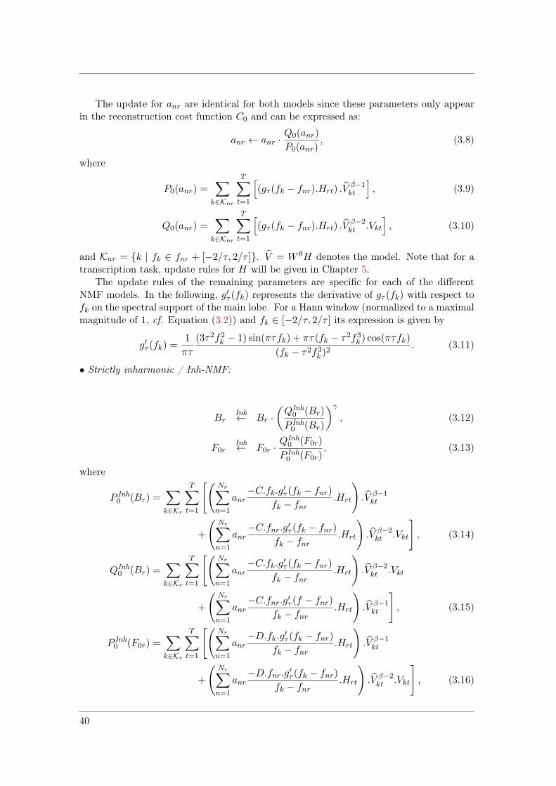
The update for anr are identical for both models since these parameters only appearin the reconstruction cost function C0 and can be expressed as:
anr ← anr ·Q0(anr)
P0(anr), (3.8)
where
P0(anr) =∑
k∈Knr
T∑
t=1
[(gτ (fk − fnr).Hrt) .V
β−1kt
], (3.9)
Q0(anr) =∑
k∈Knr
T∑
t=1
[(gτ (fk − fnr).Hrt) .V
β−2kt .Vkt
], (3.10)
and Knr = k | fk ∈ fnr + [−2/τ, 2/τ ]. V = W θH denotes the model. Note that for atranscription task, update rules for H will be given in Chapter 5.
The update rules of the remaining parameters are specific for each of the differentNMF models. In the following, g′τ (fk) represents the derivative of gτ (fk) with respect tofk on the spectral support of the main lobe. For a Hann window (normalized to a maximalmagnitude of 1, cf. Equation (3.2)) and fk ∈ [−2/τ, 2/τ ] its expression is given by
g′τ (fk) =1
πτ
(3τ2f2k − 1) sin(πτfk) + πτ(fk − τ2f3
k ) cos(πτfk)
(fk − τ2f3k )
2. (3.11)
• Strictly inharmonic / Inh-NMF:
BrInh← Br ·
(QInh
0 (Br)
P Inh0 (Br)
)γ
, (3.12)
F0rInh← F0r ·
QInh0 (F0r)
P Inh0 (F0r)
, (3.13)
where
P Inh0 (Br) =
∑
k∈Kr
T∑
t=1
[(Nr∑
n=1
anr−C.fk.g′τ (fk − fnr)
fk − fnr.Hrt
).V β−1
kt
+
(Nr∑
n=1
anr−C.fnr.g′τ (fk − fnr)
fk − fnr.Hrt
).V β−2
kt .Vkt
], (3.14)
QInh0 (Br) =
∑
k∈Kr
T∑
t=1
[(Nr∑
n=1
anr−C.fk.g′τ (fk − fnr)
fk − fnr.Hrt
).V β−2
kt .Vkt
+
(Nr∑
n=1
anr−C.fnr.g′τ (f − fnr)
fk − fnr.Hrt
).V β−1
kt
], (3.15)
P Inh0 (F0r) =
∑
k∈Kr
T∑
t=1
[(Nr∑
n=1
anr−D.fk.g
′τ (fk − fnr)
fk − fnr.Hrt
).V β−1
kt
+
(Nr∑
n=1
anr−D.fnr.g
′τ (fk − fnr)
fk − fnr.Hrt
).V β−2
kt .Vkt
], (3.16)
40

CHAPTER 3. ESTIMATING THE INHARMONICITY COEFFICIENT AND THE F0 OF PIANO TONES
QInh0 (F0r) =
∑
k∈Kr
T∑
t=1
[(Nr∑
n=1
anr−D.fk.g
′τ (fk − fnr)
fk − fnr.Hrt
).V β−2
kt .Vkt
+
(Nr∑
n=1
anr−D.fnr.g
′τ (f − fnr)
fk − fnr.Hrt
).V β−1
kt
], (3.17)
with fnr = nF0r
√1 +Brn2, C = ∂fnr/∂Br = n3F0r/2
√1 +Brn2 and D = ∂fnr/∂F0r =
n√1 +Brn2. The set of frequency-bins for which the model spectrum W
θInhr
kr is defined ishere denoted by Kr = k | fk ∈ fnr + [−2/τ, 2/τ ], n ∈ [1, Nr].One can note that an exponent γ > 0 has been included in the update of Br, in Equation(3.12). This parameter, whose role is similar to the step size in usual gradient descents,allows for the control of the convergence rate of the parameter Br [Bertin et al., 2009]. Weempirically found that setting γ = 10 was leading to accelerated updates while preservingthe decrease of the cost-function.
• Inharmonic relaxed / InhR-NMF:
For the inharmonic relaxed model, the following update rules are applied. Note thatfor F0r, an exact analytic solution is obtained when canceling the partial derivative of thecost-function C1 (Equation (3.7)).
fnrInhR← fnr ·
QInhR0 (fnr) + λ ·QInhR
1 (fnr)
P InhR0 (fnr) + λ · P InhR
1 (fnr), (3.18)
BrInhR← Br ·
QInhR1 (Br)
P InhR1 (Br)
, (3.19)
F0rInhR=
Nr∑n=1
fnrn√1 +Brn2
Nr∑n=1
n2(1 +Brn2)
, (3.20)
where
P InhR0 (fnr) =
∑
k∈Knr
T∑
t=1
[(anr−fk.g′τ (fk − fnr)
fk − fnr.Hrt
).V β−1
kt
+
(anr−fnr.g′τ (fk − fnr)
fk − fnr.Hrt
).V β−2
kt .Vkt
], (3.21)
QInhR0 (fnr) =
∑
k∈Knr
T∑
t=1
[(anr−fk.g′τ (fk − fnr)
fk − fnr.Hrt
).V β−2
kt .Vkt
+
(anr−fnr.g′τ (f − fnr)
fk − fnr.Hrt
).V β−1
kt
], (3.22)
P InhR1 (fnr) = KτT · 2fnr, (3.23)
QInhR1 (fnr) = KτT · 2nF0r
√1 +Brn2, (3.24)
41

P InhR1 (Br) = F0r
Nr∑
n=1
n4, (3.25)
QInhR1 (Br) =
Nr∑
n=1
n3fnr√1 +Brn2
. (3.26)
3.1.2.2 Practical considerations
Choice of the reconstruction cost-function: As seen in Section 2.2, high rank par-tials of piano tones should be taken into account when targeting the precise estimationof (B,F0). Besides the tuning of Nr, the number of partials for a note of the model, thechoice of the reconstruction cost-function may have an influence on the precision of theestimation. For the experiments presented in this thesis a Kullback-Leibler divergence(β = 1) has been considered. This choice corresponds to a trade-off between the Euclidiandistance (β = 2), for which the estimation would mainly rely on low rank partials - thesehaving usually the greatest amplitudes in the spectrum of a note and whose frequenciesmay be affected by the bridge coupling - and the Itakura-Saito divergence (β = 0) thatwould consider every partial regardless of its amplitude, even high rank partials that maybe drowned out in noise.
Initialization of the parameters: A good initialization of the optimization algorithmcorresponds to the overlap of an important number of partials between the model and thedata. As shown in Figure 3.1(a), a naive initialization (F0 set to Equal Temperament andB to a common value for every note) may lead to the overlap of only a few first partialsand cause the algorithm to stop in a local minimum.
In order to avoid these situations, special care is taken to initialize (Br, F0r). Thislatter is performed using a model for the inharmonicity and the tuning of pianos along thewhole compass, with typical values of the parameters. This model, presented in Chapter4, is based on generic rules in design and tuning. One can see on Figure 3.1(b) that suchinitialization leads to the overlap of a greater number of partials (20 for this example).However, it can be noticed around 1400 Hz that partials of the model are overlapping withsome partials of the data with different ranks. This situation may correspond to a localminimum of the reconstruction cost-function.
Thus, it is chosen for the algorithm to initialize the spectra of the model with a fewpartials (it is empirically chosen that N ini
r decreases linearly from 10 for lowest notes to2 for highest, as displayed with gray ‘+’ markers on Figure 3.2). The number of partialsis then iteratively increased after each update of (Br, F0r) until the maximum numberof partials Nfin
r is reached (cf. black ‘+’ markers on Figure 3.2, where for each note ofthe model the maximum number of partials below the Nyquist frequency limit is set to50). This heuristic should broaden the zone where the cost-function is convex in order toiteratively converge toward optimal values of the parameters (cf. Figure 3.3). It has beenexperimentally chosen for the following experiments to add one partial for every note ofthe model every 3 iterations of the optimization loop.
42

CHAPTER 3. ESTIMATING THE INHARMONICITY COEFFICIENT AND THE F0 OF PIANO TONES
0 200 400 600 800 1000 1200 1400 1600 1800 2000 2200
−100
−80
−60
−40
−20
0
Frequency (Hz)
Mag. spectr
um
(dB
)
Observation
Model
(a)
0 200 400 600 800 1000 1200 1400 1600 1800 2000 2200
−100
−80
−60
−40
−20
0
Frequency (Hz)
Mag. spectr
um
(dB
)
Observation
Model
(b)
Figure 3.1: Initialization of the NMF models for the analysis of a note D1. (a) Roughinitialization with F0 set to Equal Temperament and B = 5.10−3. (b) Initialization usingthe model of inharmonicity and tuning along the whole compass of pianos.
0 10 20 30 40 50 60 70 80 900
10
20
30
40
50
60
r (note index)
Nr (
pa
rtia
l n
um
be
r)
Nr
ini
Nr
fin
Nr
lim
Figure 3.2: Number of partials Nr for the 88 notes of the models (r ∈ [1, 88], from A0 toC8) at the initialization (gray markers labeled as N ini
r ) and at the end of the algorithm(black markers labeled as Nfin
r , here depicted for a choice of 50 partials maximum). Theblack dashed curve labeled as N lim
r corresponds to the maximum number of partials thatshould be present below the Nyquist frequency (with a sampling frequency of 22050 Hz).For notes in the bass range this limits, not displayed here, goes up to around 180 partials.
43

log10
B
F0/F
0,E
T (
ce
nts
)
−5 −4.8 −4.6 −4.4 −4.2 −4 −3.8 −3.6
−30
−25
−20
−15
−10
−5
0
5
10
15
1600
1700
1800
1900
2000
2100
2200
2300
2400
2500
2600min
ini
(a) Nr = 10
log10
B
F0/F
0,E
T (
ce
nts
)
−5 −4.8 −4.6 −4.4 −4.2 −4 −3.8 −3.6
−30
−25
−20
−15
−10
−5
0
5
10
15
7000
7500
8000
8500
9000
9500
min
ini
(c) Nr = 30
log10
B
F0/F
0,E
T (
ce
nts
)
−5 −4.8 −4.6 −4.4 −4.2 −4 −3.8 −3.6
−30
−25
−20
−15
−10
−5
0
5
10
15
4200
4400
4600
4800
5000
5200
5400
5600
5800
6000min
ini
(b) Nr = 20
log10
B
F0/F
0,E
T (
ce
nts
)
−5 −4.8 −4.6 −4.4 −4.2 −4 −3.8 −3.6
−30
−25
−20
−15
−10
−5
0
5
10
15
1.35
1.4
1.45
1.5
1.55
1.6
x 104
min
ini
(d) Nr = 50
Figure 3.3: Cost-function for Inh-NMF (Eq. (3.5) with β = 1) computed on a grid of(Br, F0r), and different numbers of partials Nr, having amplitudes anr fixed to 1, for theanalysis of the spectrum of a note D1. Black and gray markers respectively correspond tothe initialization and the minimum of the cost-function.
Discussion about the tuning of the regularization parameter for InhR-NMF :As mentioned in Section 3.1.1.2, the tuning of the regularization parameter λ influences theweighting between the reconstruction cost-function C0 and the inharmonicity constraintC1. A too high value of λ will favor a good fit of the partial frequencies with the inhar-monicity relation without considering the slight deviations, e.g. due to the soundboard-string couplings, while a too small value will lead to an optimal reconstruction of thespectrum, even if the partials of the model do not match with transverse vibration par-tials. The influence of the tuning of λ for a given partial is illustrated on Figure 3.4. Forthis particular example, the optimal values of fnr are different for C0 and C1 cost-functions(these are depicted, respectively as dash-dotted and dashed vertical lines). While increas-ing λ from 0 to 1, one can see on Figure 3.4(b) that the global minimum of CInhR ischanging from the optimal value of C0 to the one of C1. In this example, the differencebetween the values of these two optima is coming from the fact that the partial frequencyactually deviates from the inharmonicity relation. In this case, a value of λ ∈ [10−4, 10−3]should allow a good match of the partial of transverse vibrations with the observation(i.e minimize C0), while avoiding the local minima of C0 (as can be seen on Figure 3.4(c)around 1380 or 1412 Hz for λ = 0).
44

CHAPTER 3. ESTIMATING THE INHARMONICITY COEFFICIENT AND THE F0 OF PIANO TONES
1380 1390 1400 1410 1420 1430−100
−80
−60
−40
−20
0
Frequency (Hz)
Mag. spectr
um
(dB
)
ObservationPartial of the model (for a given f
nr)
min C0
min C1
(a)
1380 1390 1400 1410 1420 14300
2000
4000
6000
8000
10000
12000
14000
16000
fnr
grid (Hz)
CIn
hR
λ = 0
λ = 10−4
λ = 10−3
λ = 10−2
λ = 10−1
λ = 1min C
0
min C1
(b)
1380 1390 1400 1410 1420 14304000
4500
5000
5500
fnr
grid (Hz)
CIn
hR
λ = 0
λ = 10−4
λ = 10−3
λ = 10−2
λ = 10−1
λ = 1min C
0
min C1
(c)
Figure 3.4: Influence of the tuning of λ on the cost-function of InhR-NMF. (a) Partial oftransverse vibration of a spectrum (gray) and partial of the model (black) for a given fnrand anr = 1. (b) Corresponding cost-function CInhR (Eq. (3.6)) computed on a grid offnr for anr fixed to 1 and different values of λ. (c) Zoom along the y-axis of sub-figure(b). Vertical dashed-dot and dashed line bars correspond to the value of fnr, respectively,minimizing C0 and C1.
Since we use a Kullback-Leibler divergence for the reconstruction cost-function C0, oneshould note that the tuning of λ may be influenced by the amplitude of the partials of theobservations. Indeed, the Kullback-Leibler divergence is not scale invariant and dKL(γx |γy) = γ dKL(x | y), γ ∈ R
+. In order to avoid a fine tuning of λ that depends on therecording conditions (piano type, nuances, ...) each spectrum composing the observationmatrix is normalized to a maximal magnitude of 1. Thus, the illustrations of Figure 3.4correspond to the tuning of λ for a partial with maximal amplitude. When considering apartial with amplitude 0.1 (-20 dB), a similar network of curves of Figure 3.4(b) will beobtained by multiplying every value of λ by 10. For the experiments that are presentedin Section 3.1.3, λ has been set empirically λ = 5 · 10−4.
45

Dealing with noise: In theory, when analyzing piano tones, one should consider partialsin the whole frequency range. Thus, the number of partials having frequencies below theNyquist frequency Fs/2 (Fs being the sampling frequency) should be given, for each note,by:
N limr =
Fs
2F0r
√√√√2
1 +√
1 +BrF 2s
F 20r
, (3.27)
where ⌊.⌋ denotes the integer rounding towards −∞ (as depicted in black line on Fig-ure 3.2). However in practice, some partials, mainly with high ranks, may be missing ordrowned out in noise because of their strong damping. When targeting the precise estima-tion of (B,F0), taking into account these partials in the model may lead to bad estimates.Thus, for each iteration of the optimization algorithm, we cancel their influence in the es-timation of (Br, F0r) by removing them from the corresponding cost-functions (Eq. (3.5)for Inh-NMF and Eq. (3.7) for InhR-NMF ). For the proposed application, we compute,during a pre-processing step, the noise level NL(fk) on each magnitude spectrum compos-ing the matrix V (see Appendix B), and at each iteration we look for the estimated partialsthat have a magnitude greater than the noise. Thus, we define the set of reliable partialsof each note, being above the noise level, by ∆r = n | anr > NL(fnr), n ∈ [1, Nr].This information is taken into account by replacing the sums over the entire set of partialsNr∑n=1
by sums over the reliable set of partials∑
n∈∆r
in the update rules of Br (Eq. (3.14)-
(3.15) for Inh-NMF, and Eq. (3.25)-(3.26)) for InhR-NMF ) and F0r (Eq. (3.16)-(3.17) forInh-NMF and Eq. (3.20) for InhR-NMF ).
3.1.2.3 Algorithms
Finally, the steps of Inh-NMF and InhR-NMF algorithms are summarized, respectivelyin tables Algorithm 1 and Algorithm 2. Note that the number of iterations for eachparameter has been determined empirically.
46

CHAPTER 3. ESTIMATING THE INHARMONICITY COEFFICIENT AND THE F0 OF PIANO TONES
Algorithm 1 Inh-NMF for the estimation of (B,F0)
1: Input:
2: V set of magnitude spectra (each normalized to a max. of 1)3: H filled with 0 and 14: β = 1
5: Pre-processing:
6: for each column of V compute NL(fk) the noise level (cf. App. B)
7: Initialization:
8: (Br, F0r), ∀ r ∈ [1, R] according to the model of Sec. 4.4.39: N ini
r and Nfinr , ∀ r ∈ [1, R] as shown in Fig. 3.2
10: fnr = nF0r
√1 +Brn2, anr = 1, ∀ r ∈ [1, R], n ∈ [1, N ini
r ]11: W θ computation (cf. Eq. ((3.1))
12: Optimization:
13: for it = 1 to It do
14: if mod(it, 3) = 0 then
15: Nr ← Nr + 1, ∀r ∈ [1, R] provided Nr < Nfinr
16: end if
17: • anr update ∀ r ∈ [1, R], n ∈ [1, Nr] (Eq. (3.8))18: W θ update (Eq. (3.1))19: deduce ∆r by comparing anr with NL(fnr)20: for u = 1 to 10 do
21: • F0r update ∀r, n ∈ ∆r (cf. Eq. (3.13))22: W θ update (cf. Eq. ((3.1))23: • Br update ∀r, n ∈ ∆r (cf. Eq. (3.12))24: W θ update (cf. Eq. ((3.1))25: end for
26: end for
27: Output: Br, F0r, anr
Algorithm 2 InhR-NMF for the estimation of (B,F0)
1: Input:
2: V set of magnitude spectra (each normalized to a max. of 1)3: H filled with 0 and 14: β = 1 / λ = 5 · 10−4
5: Pre-processing:
6: for each column of V compute NL(fk) the noise level (cf. App. B)
7: Initialization:
8: (Br, F0r), ∀ r ∈ [1, R] according to the model of Sec. 4.4.39: N ini
r and Nfinr , ∀ r ∈ [1, R] as shown in Fig. 3.2
10: fnr = nF0r
√1 +Brn2, anr = 1, ∀ r ∈ [1, R], n ∈ [1, N ini
r ]11: W θ computation (cf. Eq. ((3.1))
12: Optimization:
13: for it = 1 to It do
14: if mod(it, 3) = 0 then
15: Nr ← Nr + 1, ∀r ∈ [1, R] provided Nr < Nfinr
16: end if
17: • anr update ∀ r ∈ [1, R], n ∈ [1, Nr] (Eq. (3.8))18: W θ update (Eq. (3.1))19: deduce ∆r by comparing anr with NL(fnr)20: • fnr update ∀ r ∈ [1, R], n ∈ [1, Nr] (Eq. (3.18))21: W θ update (Eq. (3.1))22: for v = 1 to 30 do
23: ∀r, n ∈ ∆r
24: F0r update (cf. Eq. (3.20))25: Br update (20 times) (cf. Eq. (3.19))26: end for
27: end for
28: Output: Br, F0r, anr, fnr
47

3.1.3 Results
The ability of both NMF models/algorithms to provide correct estimates of (B,F0) onthe whole piano compass is investigated here in a supervised context (i.e. the playednotes and their time-activations are known). The estimation from isolated note and chordrecordings are respectively presented in Sections 3.1.3.2 and 3.1.3.4.
3.1.3.1 Database presentation
The results presented in this section are obtained from 3 separate databases (Iowa [Uni-versity of Iowa, 1997], RWC [Goto et al., 2003] and MAPS [Emiya et al., 2010b]) coveringa total of 11 different pianos with different recording conditions (microphones close tothe strings or in room ambient condition) and dynamics (piano, mezzo-forte, forte). Thedetails for all pianos are given in Table 3.1. Note, that all piano synthesizers from MAPSdatabase are using high-quality samples. For all pianos, isolated note recordings alongthe whole compass, from A0 (21 in MIDI index)1 to C8 (108), are available. For MAPSpianos, chord recordings are also given. An additional dataset [Rauhala et al., 2007a]composed of synthesized isolated tones from A0 (21) to G3 (55) is used in Section 3.1.3.3for the evaluation of the precision of B estimates.
ref. name piano type rec. conditions
Iowa Iowa grand close
RWCRWC1 grand closeRWC2 grand closeRWC3 grand close
MAPS
AkPnBcht grand (synth.) Software presetAkPnBsdf grand (synth.) Software preset
AkPnCGdD grand (synth.) Software presetAkPnStgb upright (synth.) Software preset
ENSTDkAmupright
ambiantENSTDkCl closeSptkBGAm
grand (synth.)ambiant
SptkBGCl closeStbgTGd2 grand (synth.) Software preset
Table 3.1: Details of the databases.
3.1.3.2 Isolated note analysis
The dataset for each piano consists of isolated note recordings of the 88 notes composingthe compass. Each recording is here first down-sampled to Fs = 22050 Hz. In order toobtain a sufficient spectral resolution for notes in the bass range, the observation spectraare extracted from 300 ms Hann windows, applied to the decay part of the sounds. Then,the matrix V is built by concatenating the 88 spectra (each column corresponding tothe magnitude spectrum of a note, from A0 (21) to C8 (108)) and H is fixed to theidentity matrix (cf. Figure 3.5). For each note, the number of partials Nr is set toargminNr
(50, fNr,r < Fs/2), as depicted in black ‘+’ markers on Figure 3.2.
1In the following, each note is given with its MIDI note number in brackets. More details on the MIDInorm are given in Appendix A.
48

CHAPTER 3. ESTIMATING THE INHARMONICITY COEFFICIENT AND THE F0 OF PIANO TONES
Figure 3.5: Scheme for the NMF-based estimation of (B,F0) along the whole compass ofpianos from isolated note recordings.
It is worth noting here that the experiments have been performed for three sets ofdynamics, namely forte, mezzo-forte and piano. Only the results for the mezzo-forte dy-namics are presented in the following since the performance did not appear significantlydependent. Also, MAPS datasets are composed of tones played with different configura-tions for the forte pedal: active or inactive (randomly distributed).
Two selected examples are presented in Figures 3.6 and 3.7 in order to exhibit char-acteristics of both algorithms and analyze particular cases that lead to a failure of theestimation. The results for the 11 pianos are given in Appendix D, page 125. Sub-figures(a) correspond to the inharmonicity curves along the compass. As discussed in Chapter 4,all piano models have a similar B behavior for the highest notes. Sub-figure (b) representthe curves of F0 as the deviation from Equal Temperament (ET), in cents. The initializa-tion of (B,F0) is depicted as black dashed lines and the blue and red curves respectivelycorrespond to the estimates obtained by Inh-NMF and InhR-NMF algorithms.
20 30 40 50 60 70 80 90 100
10−4
10−3
10−2
m (note in MIDI index)
B (
log
. sca
le)
ini
Inh−NMF
InhR−NMF
(a)
20 30 40 50 60 70 80 90 100
−20
−15
−10
−5
0
5
10
15
m (note in MIDI index)
F0/F
0,E
T (
ce
nts
)
ini
Inh−NMF
InhR−NMF
(b)
Figure 3.6: Iowa (a) B and (b) F0 as dev. from ET along the whole compass.
49

20 30 40 50 60 70 80 90 100
10−4
10−3
10−2
m (note in MIDI index)
B (
log
. sca
le)
ini
Inh−NMF
InhR−NMF
(a)
20 30 40 50 60 70 80 90 100−20
−15
−10
−5
0
5
10
15
20
25
30
35
m (note in MIDI index)
F0/F
0,E
T (
ce
nts
)
ini
Inh−NMF
InhR−NMF
(b)
Figure 3.7: ENSTDkAm (a) B and (b) F0 as dev. from ET along the whole compass.
When comparing the blue and red curves one can see that for most notes, particularlyin the medium range, both estimates are in good agreement. In order to qualitativelyevaluate the results one can compare the observed spectra and the model. For instanceFigure 3.8 depicts the result of InhR-NMF algorithm for the analysis of notes C♯1 (25),C4 (60) and G♯5 (80) of Iowa grand piano. Inh-NMF exhibits similar results (not shownhere).
However, for some particular examples a significant difference between Inh-NMF andInhR-NMF estimates is visible, for instance in the bass range of ENSTDkAM piano be-tween A0 (21) and A1 (33) on Figure 3.7. When comparing the observed spectrum andthe models for the note F♯1 (cf. Figure 3.9), one can see that Inh-NMF failed to fit thepartials of transverse vibrations from rank 27 (Figure 3.9(a)), while InhR-NMF correctlyfitted the 50 partials (Figure 3.9(b)). Figure 3.9(c) shows that the failure of Inh-NMF isdue to the fact that the partial frequencies significantly differ from the theoretical inhar-monicity relation (2.23). The “+” markers correspond to a plot of the partial frequenciesobtained by InhR-NMF in the graphic (fnr/n)
2 as a function of n2. If the partial frequen-cies were strictly following the inharmonicity relation they should be distributed accordingto a straight line of equation F 2
0r(1 + Brn2). Thus, InhR-NMF here succeeds to adapt
the parameters (Br, F0r) (red straight line) during the optimization while permitting thepartials with low ranks to deviate from the theoretical law to fit the partials of the ob-servation. On the contrary, the strict constraint of Inh-NMF led to the estimation of aninharmonicity relation fitting approximately the first 27 partials (blue straight line). It isworth noting for this very particular example that the distribution of the partial frequen-cies differs from the usual inharmonicity relation with deviations caused by the bridgecoupling (as shown in Figure 2.10, page 31) and may be resulting from other effects suchas for instance the wrapping of the strings in the bass range (cf. Section 4.2.2.1). In thiscase, the validity of the estimation of (B,F0) is hardly quantifiable because the model of
50

CHAPTER 3. ESTIMATING THE INHARMONICITY COEFFICIENT AND THE F0 OF PIANO TONES
0 200 400 600 800 1000 1200 1400 1600 1800 2000 2200
−100
−80
−60
−40
−20
0
Frequency (Hz)
Mag.
Spectr
um
(dB
)
Observation
Noise Level
Model
(a)
0 1000 2000 3000 4000 5000 6000−120
−100
−80
−60
−40
−20
0
Frequency (Hz)
Mag.
Spectr
um
(dB
)
Observation
Noise Level
Model
(b)
0 1000 2000 3000 4000 5000 6000
−100
−80
−60
−40
−20
0
Frequency (Hz)
Mag. S
pectr
um
(dB
)
Observation
Noise Level
Model
(c)
Figure 3.8: Results of InhR-NMF for the analysis of notes (a) C♯1, (b) C4 and (c) G♯5 ofIowa grand piano.
transverse vibration is not sufficient to explain the distribution of the partial frequencies.However, a benefit of InhR-NMF is to handle these discrepancies so that a recovery of thecomplete set of partials is still possible.
Other differences between the results provided by both algorithms can be seen in thetreble range. For instance, Figure 3.10 depicts the result of InhR-NMF for the note B6(95) of ENSTDkAM piano. In this case, the validity of the estimation cannot be assessedso easily for some partials, mainly because these partials aggregate multiple peaks whilethe model assumes only a single component. This issue typically happens in the treblerange, where the notes are associated with triplets of slightly detuned strings. Then,the algorithm selects one peak per group, that will depend on the initialization and ona balance between peak strength and model fitting. Thus, each algorithm might returnslightly different biased estimates for (B,F0), depending on which partials are selected.
Finally, in some cases corresponding mainly to notes in the high treble range, bothalgorithms may fail because of initialization issues. This can be seen of Figure 3.6 wherethe estimates of (B,F0) for notes above G7 (103) remain fixed to their initial values becauseno partials of the models were overlapping partials of the data at the initialization. Forinstance, a difference of 10 cents between the initialization and the actual value of F0 of
51

a note G7 leads approximately to a deviation of 18 Hz between the first partial frequencyof the observation and the model. In order that the main lobes of the first partial of theobservation and the model overlap at the initialization, the limit deviation between thepartial frequencies is equal to 4/τ for a Hann window. For the presented results, a 300ms Hann window was used so this limit is approximately equal to 13 Hz. Under theseconditions, it is very likely that no partial of the model overlaps partials of the observedspectrum at the initialization, thus leading to a failure of both algorithms. Similar resultsmay be observed for AkPnBcht and AkPnBsdf in Appendix D. A possible solution toovercome these limitations is to perform a rough estimation by means of a grid searchbefore running the optimization. Also, using a shorter analysis window may help inincreasing the overlapping between the observed and modeled partials (for instance a 50ms Hann window will lead to a limit of 80 Hz).
0 500 1000 1500 2000 2500
−100
−80
−60
−40
−20
0
Frequency (Hz)
Ma
g.
Sp
ectr
um
(d
B)
Observation
Noise Level
Model Inh−NMF
(a)
0 500 1000 1500 2000 2500
−100
−80
−60
−40
−20
0
Frequency (Hz)
Ma
g.
Sp
ectr
um
(d
B)
Observation
Noise Level
Model InhR−NMF
(b)
0 500 1000 1500 2000 25002000
2100
2200
2300
2400
2500
2600
2700
2800
n2
(fnr
InhR / n)
2
(F0r
InhR)2 (1 + B
r
InhR n
2)
(F0r
Inh) 2
(1 + Br
Inh n
2)
(c)
Figure 3.9: Estimation of (B,F0) for the note F♯1 (30) of MAPS ENSTDkAM piano.Observed spectrum and estimated spectrum by (a) Inh-NMF and (b) InhR-NMF. (c)Plot (fnr/n)
2 as a function of n2, with the inharmonicity relation estimated by Inh-NMFand InhR-NMF, respectively depicted as blue and red lines.
52

CHAPTER 3. ESTIMATING THE INHARMONICITY COEFFICIENT AND THE F0 OF PIANO TONES
Figure 3.10: Results of InhR-NMF for the note B6 (95) of ENSTDkAM piano.
3.1.3.3 Performance evaluation
This section presents the quantitative evaluation of the precision of the estimation of(B,F0) provided by both algorithms and a comparison with the state-of-the-art PFD(Partial Frequencies Deviation) algorithm [Rauhala et al., 2007a; Rauhala and Välimäki,2007].
Reference extraction: The evaluation is performed on both synthetic and Iowa realpiano tones on the limited range A0 (21) - G3 (55) (as done in [Rauhala et al., 2007a])because of the lack of ground truth. Indeed, the string dimensions and properties are notknown for real pianos so the reference values of B need to be manually retrieved from thenote spectra. This requires a supervised extraction of the partial frequencies correspondingto transverse vibrations of the strings, which can be quite difficult because of the presenceof many partials due to the string couplings, particularly for notes composed of multiplestrings. In our experiments, the partials corresponding to transverse vibrations of thestrings have been picked, up to a rank of 30, from the spectra of notes played withpiano dynamics so that the influence of the couplings should be limited. In order tohave a precise spectral resolution, the spectra have been computed from 2 seconds ofdecaying sound on 217 frequency bins. In case multiple partials are produced by thecoupling of doublet/triplet of strings, several peaks have been considered (as illustratedon Figure 3.11(a)). In the following equation, the frequencies of these peaks are denotedby f⋆
r,n,p, where r corresponds to the index of the note, p ∈ [1, Pr,n] to the index ofthe peak within n ∈ [1, Nr] the rank of the partial. Then, the reference parameters(B⋆
r , F⋆0r) have been estimated by minimizing the absolute deviation (which should reduce
the influence of potential outliers) between the inharmonicity relation and the extractedpartial frequencies:
(B⋆r , F
⋆0r) = argmin
(Br,F0r)
Nr∑
n=1
Pr,n∑
p=1
1
Pr,n| f∗r,n,p − nF0r
√1 +Brn2 | . (3.28)
The 1/Pr,n factor corresponds to a weighting that allows us to consider multiple partials asone theoretical partial in the regression. The result of the estimation of (B⋆, F ⋆
0 ) for G♯2note of Iowa grand piano is depicted in Figure 3.11(b) by plotting (fn/n)
2 as a functionof n2. Finally, the curves of B⋆
r and F ⋆0r (as deviation from ET) are presented for both
datasets along the range A0 (21) - G3 (55) in Figure 3.12.
53

(a)
0 100 200 300 400 500 600 700 800 900
1.08
1.1
1.12
1.14
1.16
1.18
1.2x 10
4
n2
f n2 / n
2
Peaks
Estimated inh. relation
(b)
Figure 3.11: (B,F0) reference extraction on note G♯2 of Iowa grand piano. (a) Magnitudespectrum (in gray), and selection of the peaks corresponding to transverse vibrations ofthe strings (’+’ markers). (b) Results of the estimation of (B⋆, F ⋆
0 ) reference values in theplane (fn/n)
2 as a function of n2. ‘+’ markers correspond to manually extracted peaks,and gray line to the estimated inharmonicity relation.
20 25 30 35 40 45 50 55
1
2
3
note (in MIDI index)
B* (
log
. sca
le)
x10−4
20 25 30 35 40 45 50 55−1
−0.8
−0.6
−0.4
−0.2
0
0.2
0.4
0.6
0.8
1
note (in MIDI index)
F0* /
F0,E
T (
ce
nts
)
(a) Synthetic
20 25 30 35 40 45 50 55
1
2
3
note (in MIDI index)
B* (
log
. sca
le)
x10−4
20 25 30 35 40 45 50 55−25
−20
−15
−10
−5
0
5
10
note (in MIDI index)
F0* /
F0,E
T (
ce
nts
)
(b) Iowa
Figure 3.12: Reference curves (B⋆, F ⋆0 ) along the range A0 (21) - G3 (55) for (a) the
synthetic samples and (b) the Iowa piano tones.
54

CHAPTER 3. ESTIMATING THE INHARMONICITY COEFFICIENT AND THE F0 OF PIANO TONES
Evaluation results: The inharmonicity coefficient estimation performances are evalu-ated in terms of relative error with respect to the reference:
EBr =∣∣∣Br −B⋆
r
B⋆r
∣∣∣. (3.29)
F0 estimates are evaluated in terms of deviation from the reference in cents:
EF0r = 1200 ·∣∣∣log2
F0r
F ⋆0r
∣∣∣. (3.30)
These measures for PFD and the two NMF algorithms are presented on Figure 3.13 forthe synthetic samples and the Iowa piano tones on the range A0 (21) - G3 (55). Table 3.2returns these errors averaged for each piano and algorithm. Higher performances are ob-tained by both NMF algorithms when compared to the PFD algorithm. The performanceobtained for the synthetic tones are similar for both NMF modelings while InhR-NMF re-turns slightly better results than Inh-NMF for the analysis of Iowa grand piano samples.These results on the first data set could be explained by the fact that the synthetic toneshave been generated by using the theoretical inharmonicity relation (Equation (2.23))without considering the partial frequency deviations caused by the soundboard-stringscoupling. Results on the Iowa data set tend to show that it is worthwhile to take thesepossible deviations into account, as done by InhR-NMF.
20 25 30 35 40 45 50 550
0.5
1
1.5
2
2.5
3
3.5
4
note (in MIDI index)
EB
r (%
)
PFD
Inh−NMF
InhR−NMF
20 25 30 35 40 45 50 550
0.2
0.4
0.6
0.8
1
1.2
1.4
note (in MIDI index)
EF
0r (
cents
)
PFD
Inh−NMF
InhR−NMF
(a) Synthetic
20 25 30 35 40 45 50 550
1
2
3
4
5
6
7
8
9
10
note (in MIDI index)
EB
r (%
)
PFD
Inh−NMF
InhR−NMF
20 25 30 35 40 45 50 550
0.5
1
1.5
2
2.5
3
note (in MIDI index)
EF
0r (
cents
)
PFD
Inh−NMF
InhR−NMF
(b) Iowa
Figure 3.13: EBr (above, in %) and EF0r (below, in cents) along the range A0 (21) -G3(55) for PFD (black), Inh-NMF (blue) and InhR-NMF (red) algorithms. The evaluationis performed on (a) synthetic and (b) Iowa piano datasets.
On G♯3 (56) - C8 (108) results are not quantified because of the lack of ground truthand data for the synthetic signals. However, it can be observed graphically (c.f. Figure3.14) that NMF estimates seem more consistent with typical values than those obtainedby using PFD (not optimized there). It is worth noting that in the presented experiments,
55
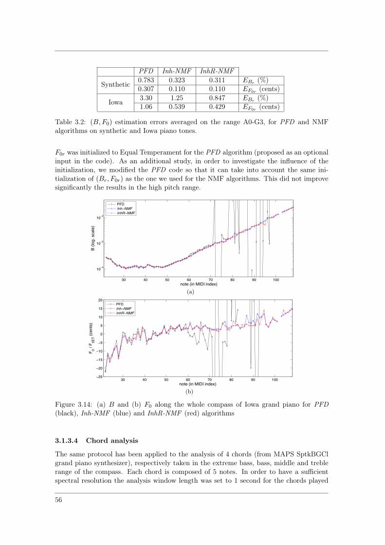
PFD Inh-NMF InhR-NMF
Synthetic0.783 0.323 0.311 EBr (%)0.307 0.110 0.110 EF0r (cents)
Iowa3.30 1.25 0.847 EBr (%)1.06 0.539 0.429 EF0r (cents)
Table 3.2: (B,F0) estimation errors averaged on the range A0-G3, for PFD and NMFalgorithms on synthetic and Iowa piano tones.
F0r was initialized to Equal Temperament for the PFD algorithm (proposed as an optionalinput in the code). As an additional study, in order to investigate the influence of theinitialization, we modified the PFD code so that it can take into account the same ini-tialization of (Br, F0r) as the one we used for the NMF algorithms. This did not improvesignificantly the results in the high pitch range.
30 40 50 60 70 80 90 100
104
103
102
note (in MIDI index)
B (
log
. sca
le)
PFD
Inh NMF
InhR NMF
(a)
30 40 50 60 70 80 90 10025
20
15
10
5
0
5
10
15
20
note (in MIDI index)
F0 /
F0
ET (
ce
nts
)
PFD
Inh NMF
InhR NMF
(b)
Figure 3.14: (a) B and (b) F0 along the whole compass of Iowa grand piano for PFD(black), Inh-NMF (blue) and InhR-NMF (red) algorithms
3.1.3.4 Chord analysis
The same protocol has been applied to the analysis of 4 chords (from MAPS SptkBGClgrand piano synthesizer), respectively taken in the extreme bass, bass, middle and treblerange of the compass. Each chord is composed of 5 notes. In order to have a sufficientspectral resolution the analysis window length was set to 1 second for the chords played
56
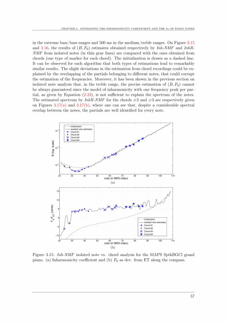
CHAPTER 3. ESTIMATING THE INHARMONICITY COEFFICIENT AND THE F0 OF PIANO TONES
in the extreme bass/bass ranges and 500 ms in the medium/treble ranges. On Figure 3.15and 3.16, the results of (B,F0) estimates obtained respectively by Inh-NMF and InhR-NMF from isolated notes (in thin gray lines) are compared with the ones obtained fromchords (one type of marker for each chord). The initialization is drawn as a dashed line.It can be observed for each algorithm that both types of estimations lead to remarkablysimilar results. The slight deviations in the estimation from chord recordings could be ex-plained by the overlapping of the partials belonging to different notes, that could corruptthe estimation of the frequencies. Moreover, it has been shown in the previous section onisolated note analysis that, in the treble range, the precise estimation of (B,F0) cannotbe always guaranteed since the model of inharmonicity with one frequency peak per par-tial, as given by Equation (2.23), is not sufficient to explain the spectrum of the notes.The estimated spectrum by InhR-NMF for the chords #2 and #3 are respectively givenon Figures 3.17(a) and 3.17(b), where one can see that, despite a considerable spectraloverlap between the notes, the partials are well identified for every note.
20 30 40 50 60 70 80 90 100 110
10−4
10−3
10−2
note (in MIDI index)
B (
log. scale
)
initialization
isolated note estimates
Chord #1
Chord #2
Chord #3
Chord #4
(a)
20 30 40 50 60 70 80 90 100 110
−10
−5
0
5
10
15
note (in MIDI index)
F0/F
ET (
cents
)
initialization
isolated note estimates
Chord #1
Chord #2
Chord #3
Chord #4
(b)
Figure 3.15: Inh-NMF isolated note vs. chord analysis for the MAPS SptkBGCl grandpiano. (a) Inharmonicity coefficient and (b) F0 as dev. from ET along the compass.
57

20 30 40 50 60 70 80 90 100 110
10−4
10−3
10−2
note (in MIDI index)
B (
log. scale
)
initialization
isolated note estimates
Chord #1
Chord #2
Chord #3
Chord #4
(a)
20 30 40 50 60 70 80 90 100 110−10
−5
0
5
10
15
note (in MIDI index)
F0/F
ET (
cents
)
initialization
isolated note estimates
Chord #1
Chord #2
Chord #3
Chord #4
(b)
Figure 3.16: InhR-NMF isolated note vs. chord analysis for the MAPS SptkBGCl grandpiano. (a) Inharmonicity coefficient and (b) F0 as dev. from ET along the compass.
0 200 400 600 800 1000 1200 1400 1600−100
−80
−60
−40
−20
0
Frequency (Hz)
Ma
g.
Sp
ectr
um
(d
B)
Observation Noise Level Gb 1 A1 C2 E2 G2
(a)
0 500 1000 1500 2000 2500 3000 3500 4000 4500−120
−100
−80
−60
−40
−20
0
Frequency (Hz)
Ma
g.
Sp
ectr
um
(d
B)
Observation Noise Level G#3 B3 D4 E4 F4
(b)
Figure 3.17: Result of InhR-NMF for the analysis of (a) the chord #2 (G1-A1-C2-E2-G2)and (b) the chord #3 (G♯3-B3-D4-E4-F4) of MAPS SptkBGCl piano.
58

CHAPTER 3. ESTIMATING THE INHARMONICITY COEFFICIENT AND THE F0 OF PIANO TONES
3.1.3.5 Conclusion
Two NMF models based on a parameterization of the dictionary for the estimation of(B,F0) have been presented so far in this chapter. The first model, denoted by Inh-NMF,forces the partial frequencies to strictly follow the theoretical inharmonicity relation, whilethe second model, denoted by InhR-NMF, relaxes this constraint by means of a weightedpenalty term added to the reconstruction cost-function. An algorithm is derived for eachmodel and special care is taken in the initialization and the optimization, in order toavoid, as much as possible, the convergence toward local optima. Both algorithms havebeen successfully applied to the supervised estimation of (B,F0) along the whole compassof different pianos from isolated note and chord recordings. Their performance evaluationcompares favorably with the state of the art PFD method, while exhibiting a benefit ofthe relaxed constraint of InhR-NMF for the analysis of real piano tones when comparedto Inh-NMF.
In Chapter 5, both models will be evaluated in a transcription task, i.e. in an unsu-pervised context, where the activation matrix H has to be estimated as well as (B,F0)and the partial amplitudes. A comparison of the performance with a simpler harmonicmodel will be performed in order to evaluate whether it is valuable to take into accountinharmonicity for such applications.
59

3.2 Probabilistic line spectrum modeling
This section introduces a probabilistic model for the analysis of line spectra – defined hereas a set of frequencies of spectral peaks with significant energy. Most algorithms dedicatedto audio applications (F0-estimation, transcription, ...) consider the whole range of audiblefrequencies to perform their analysis, while besides attack transients, the energy of musicsignals is often contained in only a few frequency components, also called partials. Thus,in a time-frame of music signal only a few frequency-bins carry information relevant forthe analysis. By reducing the set of observations, i.e. by keeping only the few mostsignificant frequency components, it can be assumed that most signal analysis tasks maystill be performed. For a given frame of signal, this reduced set of observations is herecalled a line spectrum, this appellation being usually defined for the discrete spectrum ofelectromagnetic radiations of a chemical element. In the case of piano music analysis, mostobservations should correspond to frequencies related to transverse vibration of the stringsand should allow estimating (B,F0) parameters of the played notes. Thus, it should benoticed that the proposed approach is closely related to the class of methods “Iterativepeak-picking and refinement of the inharmonicity coefficient” presented in Section 2.3.The probabilistic framework used here should help in giving a more rigorous derivation ofthe estimation algorithm and allow for performing the task in an unsupervised way.
Several studies have considered dealing with these line spectra to perform analysis.Among them, [Gómez, 2006] proposes to compute tonal descriptors from the frequenciesof local maxima extracted from polyphonic audio short-time spectra. In [Doval and Rodet,1991, 1993] a probabilistic model for multiple-F0 estimation from sets of maxima of theShort-Time Fourier Transform is introduced. It is based on a Gaussian mixture modelhaving means constrained by an F0 parameter and solved as a maximum likelihood problemby means of heuristics and grid search. Such approach has been proposed more recentlyin [Duan et al., 2010] where special care is taken to the modeling of both peaks andnon-peaks regions in order to limit the activation of spurious harmonically-related notes.The F0 parameters are estimated jointly with a candidate note selection by means of aniterative greedy search strategy. The other parameters of the model are learned frommonophonic and polyphonic training data. A similar constrained mixture model hasalso been proposed in [Kameoka et al., 2004] to model speech spectra (along the wholefrequency range, where here a Gaussian distribution is used to model the main lobe of apeak) and solved using an Expectation-Maximization (EM) algorithm.
The Probabilistic Line Spectrum (PLS ) model presented here is inspired by thesereferences. The key difference is that we focus on piano tones, which have the well-knownproperty of inharmonicity, that in turn influences tuning. This slight frequency stretchingof partials should allow, up to a certain point, disambiguation of harmonically-relatednotes. Reversely, from the set of partial frequencies, it should be possible to estimate the(B,F0) parameters while detecting the played notes. The model assumes that, for a time-frame of signal, the observations have been generated by a mixture of notes composedby partials (Gaussian mixture) and noise components. The Gaussian mixture for eachnote is constrained by (B,F0) parameters to have means distributed according to theinharmonicity relation (2.23). Then, (B,F0) parameters are estimated jointly with aclassification of each observed frequency into partial and noise classes for each note bymeans of a maximum a posteriori Expectation-Maximization algorithm. This techniqueis finally applied to the unsupervised estimation of (B,F0) along the compass of pianos,
60

CHAPTER 3. ESTIMATING THE INHARMONICITY COEFFICIENT AND THE F0 OF PIANO TONES
first in a monophonic context by jointly processing isolated note recordings, and then froma musical polyphonic piece.
3.2.1 Model and problem formulation
3.2.1.1 Observations
As mentioned in the introduction of Chapter 2, the information contained in two consec-utive frames of music signals is often highly redundant. This suggests that in order toretrieve the (B,F0) parameters for the whole set of notes played in a piece of solo music,a few independent frames localized after note onset instants should contain all the infor-mation that is necessary for processing. These time-frames are indexed by t ∈ [1, T ] in thefollowing. In order to extract peaks that contain significant energy from the magnitudespectra, a noise level estimation based on median filtering is first performed (cf. AppendixB). Above this noise level, local maxima (defined as having a greater magnitude than Kmax
left and right frequency bins) are extracted. An illustration of this pre-processing is givenin Figure 3.18. The frequency of each maximum picked in a frame t is denoted by yti,i ∈ [1, It]. The set of observations for each frame is then denoted by yt (a vector of lengthIt), and for the whole piece of music by Y = yt, t ∈ [1, T ]. In the following of thissection, the variables denoted by lower case, bold lower case and upper case letters willrespectively correspond to scalars, vectors and sets of vectors.
0 1000 2000 3000 4000 5000 6000−100
−80
−60
−40
−20
0
20
40
Frequency (Hz)
Ma
g.
Sp
ectr
um
(d
B)
Note spectrum
Noise Level
Local max.
(a)
0 1000 2000 3000 4000 5000 6000
Frequency (Hz)
(b)
Figure 3.18: Illustration of the peak-picking pre-processing. (a) Magnitude spectrum and(b) line spectrum of a note D3 (50).
3.2.1.2 Probabilistic model
If a single note of music, indexed by r ∈ [1, R], is present in a time-frame, most of theextracted local maxima should correspond to partials related by a particular structure
61

(harmonic or inharmonic for instance). These partial frequencies correspond to the setof parameters of the proposed model. It is denoted by θ, and in a general context (noinformation about the harmonicity or inharmonicity of the sounds) can be expressed byθ = fnr|∀n ∈ [1, Nr], r ∈ [1, R], where n is the rank of the partial and Nr the maximalrank for the note r. For the proposed model, we consider a strict inclusion of the inhar-monicity relation fnr = nF0r
√1 +Brn2, as done for the Inh-NMF model presented in
Section 3.1.1.2. Thus, the set of parameters can be rewritten as θ = F0r, Br|∀r ∈ [1, R].
In order to link the observations to the set of parameters θ, the following hiddenrandom variables are introduced:
• qt ∈ [1, R], corresponding to a candidate note that could have generated the obser-vations yt.
• Ct = [ctir](i,r)∈[1,It]×[1,R] gathering Bernoulli variables specifying the nature of theobservation yti, for each note r. If ctir = 1, the observation yti is assumed tocorrespond to a partial of the note r. If ctir = 0, it corresponds to "noise", heredefined as a non-sinusoidal component or a partial of another note.
• Pt = [ptir](i,r)∈[1,It]×[1,R] corresponding to the rank of the partial n of the note r thatcould have generated the observation yti provided that ctir = 1.
Based on these definitions, the probability that an observation yti has been generatedby a note r can be expressed as:
p(yti|qt = r; θ) = p(yti|ctir = 0, qt = r) · p(ctir = 0|qt = r)
+∑
n
p(yti|ptir = n, ctir = 1, qt = r; θ) (3.31)
· p(ptir = n|ctir = 1, qt = r) · p(ctir = 1|qt = r).
It is chosen that the observations that are related to the partial n of a note r should belocated around the frequencies fnr according to a Gaussian distribution of mean fnr andvariance σ2
r (fixed parameter):
p(yti|ptir = n, ctir = 1, qt = r; θ) = N (fnr, σ2r ), (3.32)
p(ptir = n|ctir = 1, qt = r) = 1/Nr. (3.33)
On the other hand, observations that are related to noise are chosen to be uniformlydistributed along the frequency axis (with maximal frequency F ):
p(yti|ctir = 0, qt = r) = 1/F. (3.34)
These distributions are illustrated on Figure 3.19.
Then, the probability to obtain a noise or partial observation knowing the note r ischosen so that:• if It > Nr:
p(ctir|qt = r) =It>Nr
(It −Nr)/It if ctir = 0,
Nr/It if ctir = 1.(3.35)
62

CHAPTER 3. ESTIMATING THE INHARMONICITY COEFFICIENT AND THE F0 OF PIANO TONES
500 600 700 800 900 1000 1100 1200 1300 1400 15000
0.005
0.01
0.015
0.02
0.025
0.03
0.035
0.04
0.045p(y
ti | c
tir=1, p
tir=3, q
t=r ; θ) p(y
ti | c
tir=1, p
tir=4, q
t=r ; θ) p(y
ti | c
tir=1, p
tir=5, q
t=r ; θ) p(y
ti | c
tir=1, p
tir=6, q
t=r ; θ)
p(yti | c
tir=0, q
t=r)
yti (Frequency Hz)
Figure 3.19: Illustration of the probabilistic model.
This should approximately correspond to the proportion of observations associated tonoise and partial classes for each note.• if It ≤ Nr:
p(ctir|qt = r) =It≤Nr
1− p if ctir = 0,
p if ctir = 1,(3.36)
with p ∈ [0, 1]. This latter expression for p < 0.5 means that for a given note r at a framet, most of observations should be mainly considered as noise if Nr (its number of partials),is greater than the number of observations It. This situation may occur for instance in aframe in which a single note from the high treble range is played. In this case, only a fewlocal maxima are extracted and lower notes, composed of much more partials, should notbe considered as present.
Finally, with no prior information it is chosen
p(qt = r) = 1/R. (3.37)
3.2.1.3 Estimation problem
In order to estimate the parameters of interest θ, the following maximum a posterioriestimation problem is solved:
(θ⋆, C⋆t t, P ⋆
t t) = argmaxθ,Ctt,Ptt
∑
t
log p(yt, Ct, Pt; θ), (3.38)
wherep(yt, Ct, Pt; θ) =
∑
r
p(yt, Ct, Pt, qt = r; θ). (3.39)
Solving problem (3.38) corresponds to the estimation of θ, jointly with a classification ofeach observation into noise or partial classes for each note. Note that the sum over t ofEquation (3.38) arises from the time-frame independence assumption (justified in Section3.2.1.1).
3.2.2 Optimization
Problem (3.38) has usually no closed-form solution but can be solved in an iterative wayby means of an Expectation-Maximization (EM) algorithm [Dempster et al., 1977]. The
63

auxiliary function at iteration (k + 1) is given by
Q(θ, Ctt, Ptt|θ(k), C(k)t t, P
(k)t t) =
∑
t
∑
r
ωrt ·∑
i
log p(yti, ctir, ptir, qt = r; θ)
(3.40)where by definition,
ωrt = p(qt = r|yt, C(k)t t, P
(k)t t; θ(k)), (3.41)
is computed at the E-step knowing the values of the parameters at iteration (k). At theM-step, θ, Ctt, Ptt are estimated by maximizing Equation (3.40). Note that the sumover i in Equation (3.40) is obtained under the assumption that in each frame the yti areindependent.
3.2.2.1 Expectation
According to Equation (3.41) and model Equation (3.31)-(3.37)
ωrt ∝It∏
i=1
p(yti, qt = r, c(k)tir, p(k)
tir; θ(k))
∝ p(qt = r) ·∏
i/ c(k)tir=0
p(yti|qt = r, c(k)tir) · p(c(k)
tir|qt = r) (3.42)
·∏
i/ c(k)tir=1
p(yti|qt = r, c(k)tir, p(k)
tir, θ(k)) · p(p(k)
tir|c(k)
tir, qt = r) · p(c(k)tir|qt = r),
normalized so that∑R
r=1 ωrt = 1 for each frame t.As defined in Equation (3.41), ωrt corresponds to the probability that a note r is active
at a frame t given the observations and the values of the parameters. Thus, the matrixΩ = [ωrt](r,t)∈[1,R]×[1,T ] is similar to the activation matrix H of NMF models.
3.2.2.2 Maximization
The M-step is performed by a sequential maximization of Equation (3.40):
• First, estimate ∀ t, i and qt = r the variables ctir and ptir. As mentioned in Section3.2.1.3, this corresponds to a classification step, where each observation is associated,for each note, to noise class (ctir = 0) or partial class with a given rank (ctir = 1 andpitr ∈ [1, Nr]). This step is equivalent to a maximization of log p(yti, ctir, ptir | qt = r; θ)which, according to Equations (3.31)-(3.37), can be expressed as:
(c(k+1)
tir , p(k+1)
tir ) = (3.43)
argmax(0,1,n)
− logF + log p(ctir = 0|qt = r),
−(yti − nF (k)
0r
√1 +B(k)
r n2)2/(2σ2r )− logNr
√2πσr + log p(ctir = 1|qt = r).
• Then, the estimation of θ is equivalent to (∀r ∈ 1...R)
(F (k+1)
0r , B(k+1)r ) = argmax
F0r,Br
∑
t
ωrt
∑
i/c(k+1)tir =1
log p(yti, c(k+1)
tir = 1, p(k+1)
tir , qt = r; θ), (3.44)
64

CHAPTER 3. ESTIMATING THE INHARMONICITY COEFFICIENT AND THE F0 OF PIANO TONES
which, according to Equations (3.31)-(3.37), leads to the following minimization problem:
(F (k+1)
0r , B(k+1)r ) = argmin
F0r,Br
∑
t
ωrt
∑
i/c(k+1)tir =1
(yti − p(k+1)
tir F0r
√1 +Br p(k+1)2
tir
)2. (3.45)
For F0r, the following update rule is obtained when canceling the partial derivative ofEquation (3.45):
F (k+1)
0r =
∑t ωrt
∑i/c
(k+1)tir =1
yti · p(k+1)
tir ·√
1 +Br p(k+1)2
tir
∑t ωrt
∑i/c
(k+1)tir =1
p(k+1)2
tir · (1 +Br p(k+1)2
tir ). (3.46)
For Br, no closed-form solution can be obtained from the partial derivative of Equation(3.45). The minimization is thus performed by means of an algorithm based on the Nelder-Mead simplex method (as implemented in the fminsearch MATLABTM function).
Algorithm 3 PLS model for the estimation of (B,F0)
Input:
vt, t ∈ [1, T ] set of magnitude spectra
Preprocessing: ∀t ∈ [1, T ]compute the Noise Level (NL) of vt (cf. App. B) and pick the frequencies yt
of the local maxima having magnitude greater than NL and Kmax left and rightfrequency bins
Initialization:
(Br, F0r), ∀ r ∈ [1, R] according to the model of Sec. 4.4.3N ini
r and Nfinr , ∀ r ∈ [1, R] as shown in Fig. 3.2, p. 43
compute ctir and ptir, ∀ t, i, r (Eq. (3.43))
Optimization:
for it = 1 to It do
if mod(it, 10) = 0 then
Nr ← Nr + 1, ∀r ∈ [1, R] provided Nr < Nfinr
end if
• E-Step:compute ωrt ∀ r ∈ [1, R], t ∈ [1, T ] (Eq. (3.42))keep the 10 highest values of ωrt in each frame t and set the others to 0normalize ωrt so that
∑r ωrt = 1 for each frame t
• M-Step:compute ctir and ptir ∀ t, i, r (Eq. (3.43))compute F0r ∀ r (Eq. (3.46))if F0r is outside the limits then fix its value to the closest limit
compute Br ∀ r (Eq. (3.45) + Nelder-Mead simplex method)if Br is outside the limits then fix its value to the closest limit
end for
Output: Br, F0r, ωrt
3.2.2.3 Practical considerations
The cost-function (cf. maximization Equation (3.38)) is non-convex with respect to(Br, F0r) parameters. Thus, as done in Section 3.1.2.2 for the NMF-based models, theinitialization of the parameters uses the model of inharmonicity and tuning of pianos alongthe whole compass (cf. Chapter 4). Also, similarly to the NMF model algorithms, theoptimization is run with a few partials for each note at the initialization. Then, one partialis added for each note every 10 iterations (number determined empirically) by initializingits frequency with the current (Br, F0r) estimates.
65

Finally, in order to avoid situations where the algorithm optimizes the parametersof a note on data corresponding to another note (e.g. increasing F0 by one semi-tone),the values of (Br, F0r) are prevented from being updated over limit curves. For B, thesecurves are presented in Section 4.4.3 and can be seen depicted as gray dashed-line inFigures 3.21(a) and 3.22(a). The limits curves for F0 are set to +/− 40 cents of theinitialization. Overfitting issues are also tackled by applying a threshold to ωrt that limitsthe polyphony level to 10 notes for each frame t. Each step of the optimization of the PLSmodel is summarized in Algorithm 3.
3.2.3 Results
In this section, we investigate the ability of the model and its algorithm to provide correctestimates of (B,F0) from the unsupervised joint analysis of a set of single note recordings,as from the analysis of a piece of polyphonic music.
The observation set is built according to the description given in Section 3.2.1.1. Thetime-frames are extracted after note onsets and their length is set to 500 ms in order tohave a sufficient spectral resolution. The FFT is computed on 215 bins and the maximaare extracted by setting Kmax = 20. Note that for the presented results, the knowledgeof the note onsets is taken from the ground truth (MIDI aligned files). For a completeblind approach, an onset detection algorithm should be first run. It can be assumed thatthis should not significantly affect these results, since onset detection algorithms usuallyperform well on percussive tones. The parameters of the model are chosen as follows :Nr is set to argminNr
(30, fNr,r < Fs/2), the parameter of the Bernoulli distribution isempirically set to p = 0.1, and σr is empirically set to 3 and 2 Hz, respectively for theapplications “isolated note estimation” and “estimation from a piece of music”.
3.2.3.1 Supervised vs. unsupervised estimation from isolated notes jointlyprocessed
Here, we apply the algorithm to the estimation of (Br, F0r) parameters from isolated noterecordings covering the whole compass of pianos. The set of observations is composed of88 frames (jointly processed), one for each note of the piano (from A0 (MIDI index 21) toC8 (108)) and processed in both supervised and unsupervised ways.
In the supervised case, the activation matrix Ω is fixed to the identity matrix (asdone in Section 3.1.3.2 for the activation matrix of the NMF-based models) and only theM-step is performed during the optimization. It is worth noting for this supervised casethat the algorithm can be seen as part of the “Iterative peak-picking and refinement ofthe inharmonicity coefficient” class of methods presented in Section 2.3. Indeed, partialscorresponding to transverse vibrations of the string are iteratively selected in the classi-fication step and (Br, F0r) are updated by minimizing the quadratic error between thepartial frequencies and the parameters. In the unsupervised case, the note activations arealso estimated by the algorithm.
The results for 2 different pianos are presented on Figure 3.21 (Iowa piano) and 3.22(MAPS SptkBGCl piano). Subplots (a) and (b) depict respectively the estimation of Band F0. When comparing the supervised (blue curves) and the unsupervised (red curves)curves one can see that similar results are obtained, approximately up to note C♯6 (85). Inthis range, one can see on subplot (c) that the matrix Ω estimated in the unsupervised caseexhibits the expected diagonal structure, up to one mistake at time-frame t = 53 for Iowa
66
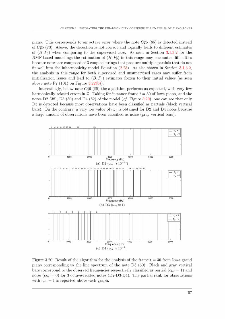
CHAPTER 3. ESTIMATING THE INHARMONICITY COEFFICIENT AND THE F0 OF PIANO TONES
piano. This corresponds to an octave error where the note C♯6 (85) is detected insteadof C♯5 (73). Above, the detection is not correct and logically leads to different estimatesof (B,F0) when comparing to the supervised case. As seen in Section 3.1.3.2 for theNMF-based modelings the estimation of (B,F0) in this range may encounter difficultiesbecause notes are composed of 3 coupled strings that produce multiple partials that do notfit well into the inharmonicity model Equation (2.23). As also shown in Section 3.1.3.2,the analysis in this range for both supervised and unsupervised cases may suffer frominitialization issues and lead to (B,F0) estimates frozen to their initial values (as seenabove note F7 (101) on Figure 3.22(b)).
Interestingly, below note C♯6 (85) the algorithm performs as expected, with very fewharmonically-related errors in Ω. Taking for instance frame t = 30 of Iowa piano, and thenotes D2 (38), D3 (50) and D4 (62) of the model (cf. Figure 3.20), one can see that onlyD3 is detected because most observations have been classified as partials (black verticalbars). On the contrary, a very low value of ωrt is obtained for D2 and D4 notes becausea large amount of observations have been classified as noise (gray vertical bars).
0 1000 2000 3000 4000 5000 6000
Frequency (Hz)
2 4 6 8 10 12 14 19 29
ctir
= 1
ctir
= 0
(a) D2 (ωrt ≈ 10−23)
0 1000 2000 3000 4000 5000 6000
Frequency (Hz)
1 2 3 4 5 6 7 8 9 10 11 12 13 14 15 16 17 18 19 20 21 22 23 24 26 27 28 29 30
ctir
= 1
ctir
= 0
(b) D3 (ωrt ≈ 1)
0 1000 2000 3000 4000 5000 6000
Frequency (Hz)
1 2 3 4 5 6 7 8
ctir
= 1
ctir
= 0
(c) D4 (ωrt ≈ 10−7)
Figure 3.20: Result of the algorithm for the analysis of the frame t = 30 from Iowa grandpiano corresponding to the line spectrum of the note D3 (50). Black and gray verticalbars correspond to the observed frequencies respectively classified as partial (ctir = 1) andnoise (ctir = 0) for 3 octave-related notes (D2-D3-D4). The partial rank for observationswith ctir = 1 is reported above each graph.
67

20 30 40 50 60 70 80 90 100
10−4
10−3
10−2
note (in MIDI index)
B (
log. scale
)
Initialization
Limits
Supervised estim.
Unsupervised estim.
(a)
20 30 40 50 60 70 80 90 100−25
−20
−15
−10
−5
0
5
10
15
20
note (in MIDI index)
F0 / F
0,E
T (
cents
)
Initialization
Supervised estim.
Unsupervised estim.
(b)
t (time frame index)
r (n
ote
in M
IDI in
dex)
10 20 30 40 50 60 70 80
30
40
50
60
70
80
90
100
0
0.1
0.2
0.3
0.4
0.5
0.6
0.7
0.8
0.9
1
(c)
Figure 3.21: Analysis on the whole compass from isolated note recordings of Iowa piano.(a) B in log. scale and (b) F0 as dev. from ET (in cents) along the whole compass. (B,F0)estimates are depicted as blue and red ‘+’ markers, respectively for the supervised andthe unsupervised cases. The initialization is plotted as gray lines and the limits for theestimation of B as gray dashed-lines. (c) Ω returned by the unsupervised analysis.
68

CHAPTER 3. ESTIMATING THE INHARMONICITY COEFFICIENT AND THE F0 OF PIANO TONES
20 30 40 50 60 70 80 90 100
10−4
10−3
10−2
note (in MIDI index)
B (
log. scale
)
Initialization
Limits
Supervised estim.
Unsupervised estim.
(a)
20 30 40 50 60 70 80 90 100−15
−10
−5
0
5
10
15
note (in MIDI index)
F0 / F
0,E
T (
cents
)
Initialization
Supervised estim.
Unsupervised estim.
(b)
t (time frame index)
r (n
ote
in
MID
I in
de
x)
10 20 30 40 50 60 70 80
30
40
50
60
70
80
90
100
0
0.1
0.2
0.3
0.4
0.5
0.6
0.7
0.8
0.9
1
(c)
Figure 3.22: Analysis on the whole compass from isolated note recordings of MAPS SP-tkBGCl piano. (a) B in log. scale and (b) F0 as dev. from ET (in cents) along the wholecompass. (B,F0) estimates are depicted as blue and red ‘+’ markers, respectively for thesupervised and the unsupervised cases. The initialization is plotted as gray lines and thelimits for the estimation of B as gray dashed-lines. (c) Ω returned by the unsupervisedanalysis.
69

Finally, the precision of the estimation of (B,F0) is quantitatively evaluated accordingto the protocol described in Section 3.1.3.3. The results are presented in table 3.3 andcompared with PFD and Inh-NMF algorithms. As qualitatively noticed above, the resultsfor both supervised and unsupervised cases are similar, and comparable to those obtainedby Inh-NMF.
PFD Inh-NMF PLS sup. PLS unsup.
Synthetic0.783 0.323 0.307 0.307 EBr (%)0.307 0.110 0.291 0.293 EF0r (cents)
Iowa3.30 1.25 1.06 1.06 EBr (%)1.06 0.539 0.607 0.601 EF0r (cents)
Table 3.3: (B,F0) estimation errors averaged on the range A0-G3, for both supervisedand unsupervised PLS (Probabilistic Line Spectrum) models applied on the synthetic andIowa piano datasets. PFD and Inh-NMF results are given for comparison. The metricsare defined in Section 3.1.3.3.
3.2.3.2 Unsupervised estimation from musical pieces
Finally, the algorithm is applied to an excerpt of polyphonic music (25 s of MAPS_MUS-muss_3_SptkBGCl file) containing notes in the range D♯1 (27) - F♯6 (90) from which46 frames are extracted. The mean polyphony level by frame is approximately equal to10.5. This high value results from the high time-frame duration which is set to 500 ms inorder to obtain a sufficient resolution, as mentioned above. 76 notes are considered in themodel and initialized in order to take into account notes from A0 (21) to C7 (96). Thiscorresponds to a reduction of one octave in the high treble range where the notes cannotbe properly processed, as seen in Section 3.2.3.1. Luckily, these notes are rarely used in amusical context.
The proposed application is here the learning of (B,F0) along the compass of a pianofrom a generic polyphonic piano recording. After the optimization, a post-processing isperformed in order to keep the most reliable estimates. First, a threshold is applied tothe matrix Ω so that elements having values lower than 10−3 (threshold set empirically)are discarded. Second, notes having B estimates stuck to the limits (cf. gray dashed linesin Figure 3.22(a)) are rejected.
Figure 3.23 depicts the result of the frame-wise note selection obtained after the post-processing for the considered piece of music. As it can be seen, the drastic post-processingleads to a greater number of True Positive (TP) than False Positive (FP). The frame-wiseevaluation returns thus a high precision of 95.7 % and a weak recall of 9.28 % (these met-rics are properly defined in Chapter 5). This result is suitable regarding our applicationfor which we mainly focus on the reliable detection of a few notes in each frame in order toperform the precise estimation of their parameters (B,F0). In a potential application ofthe algorithm to a transcription task, one should consider a smaller time-frame duration(leading to a lower frame-wise polyphony level) and a lower value for the threshold of theactivation matrix Ω at the post-processing.
Finally, the results of the estimation of (B,F0) for the detected note is presented
70

CHAPTER 3. ESTIMATING THE INHARMONICITY COEFFICIENT AND THE F0 OF PIANO TONES
FP
TP
FN
TN
t (time frame index)
no
te (
in M
IDI
ind
ex)
5 10 15 20 25 30 35 40 45
30
40
50
60
70
80
90
Figure 3.23: Frame-wise evaluation of the note detection.
on Figure 3.24 (red ‘+’ markers). When comparing to the estimates obtained by thesupervised analysis on isolated note recordings (black ‘+’ markers) one can see that mostestimates of notes actually present are consistent. Averaged on these 19 notes correctlydetected (present below note B5 (83)) and compared to the supervised estimation fromisolated note recordings, a relative error of 5.2 % for B and a mean deviation of 0.70 centsfor F0 are obtained.
Even if only a few notes are detected (19 out of 39 actually present in the presentedexample), the algorithm returned precise estimates of (B,F0). By using a model of inhar-monicity and tuning along the whole compass of pianos, it will be shown in the applicationsof Chapter 4 that (B,F0) may be interpolated along the whole compass, thus leading toapplications such as the retrieval of the tuning (related to F0) and properties about thepiano type (related to B) by the analysis of a generic polyphonic recording. Interestingly,for this task a perfect transcription of the music does not seem necessary: only a few re-liable notes may be sufficient. However, an extension of this model to piano transcriptioncould form a natural extension, but would require a more complex model taking accountboth temporal dependencies between frames, and spectral envelopes.
71

20 30 40 50 60 70 80 90 100
10−4
10−3
10−2
note (in MIDI index)
B (
log.
scale
)
Initialization
Limits
Reference
Unsupervised est.
(a)
20 30 40 50 60 70 80 90 100
−5
0
5
10
15
note (in MIDI index)
F0 / F
0,E
T (
in c
ents
)
Initialization
Reference
Unsupervised est.
(b)
20 30 40 50 60 70 80 90 100
note (in MIDI index)
present notes
detected notes
(c)
Figure 3.24: (B,F0) estimation along the compass from a piece of music. (a) B in log.scale and (b) F0 as dev. from ET in cents. (B,F0) estimates are depicted as red ‘+’markers and compared to the supervised estimation on isolated notes (black ‘+’ markers).The initialization is plotted as gray lines and the limits for the estimation of B as graydashed-lines. (c) Notes detected by the algorithm (red) and notes actually present in thepiece (black).
72

Chapter 4
A parametric model for theinharmonicity and tuning along the
whole compass of the piano
This chapter introduces a model for the variations of (B,F0) parameters along the wholecompass of pianos based on instrumental design and tuning rules. Portions of this workhave been published in [Rigaud et al., 2011, 2013a].
Most of the tuning rules related to a musical temperament are based on the controlof beatings produced when playing different intervals, these assuming that the tones areharmonic [Rasch and Heetvelt, 1985]. In the case of the piano, these beatings cannotbe exactly complied because of the partial frequency deviations inherent to the inhar-monicity. The amount of inharmonicity being dependent on the physical characteristicsof the strings, it is different for each note and type of piano. Thus, the fine tuning ofpianos is usually done aurally and requires the expertise of a professionally-skilled tunerunlike many string instruments such as guitar or cello, for which simple devices (so-called“tuners”) can be used. According to the model of piano and the choices/abilities of thetuner, the resulting tuning is unique, but within some physically-based constraints. Froma musical acoustics perspective its modeling is hence an interesting challenge that has beentackled by different viewpoints. A simulation of aural piano tuning has been proposed in[Lattard, 1993] to help pianists in tuning their own pianos, replicating the tuner’s work byiteratively tuning different intervals. The method is based on a mathematical computationof the beat rates, and requires the frequencies of the first 5 partials of each note. Morerecently, an approach using psychoacoustic principles has been introduced in [Hinrichsen,2012]. This algorithm adjusts the 88 notes at the same time, by an optimization procedureon modified spectra of the notes according to psycho-acoustic laws and tuning updates.
Our approach is different, as it jointly models tuning and inharmonicity laws for thewhole compass from a reduced set of parameters (6 mid-level parameters instead of 88×2 parameters corresponding to (B,F0) along the whole compass). Although such aninterpolated model can only capture the main trends in the inharmonicity and tuning ofa given piano, it should be reminded that one of the objectives of piano manufacturingand tuning is precisely to have a timbre that is as homogeneous as possible, smoothingout as much as possible the discontinuities of physical origins: bass break (transitionbetween treble and bass bridge), change in the number of strings per note, change ofstring diameter and winding. Therefore, it is not only realistic, but also relevant, to tryto globally parametrize the inharmonicity and tuning with only a few parameters, at leastas a first-order approximation.
The obtained synthetic description of a particular instrument, in terms of its tuning
73

/ inharmonicity pattern, can be useful to assess its state and also provides clues on someof the tuner’s choices. In the field of musical acoustics, the use of such a model couldbe helpful for instance for the tuning of physically-based piano synthesizers, where weare otherwise faced with the problem of having to adjust a large number of parameters,all of them being inter-dependent. Here a higher-level control can be obtained, witha few physically meaningful parameters. In the fields of audio signal processing andMusic Information Retrieval, including a priori knowledge is often done when trying toenhance the performance of the algorithms (cf. Section 2.3) and such models could beused to provide a good initialization of (B,F0) parameters (as done in Chapters 3 and5) and to constrain their estimation. Also, the models may be used for interpolating theinharmonicity and tuning along the whole compass of a given piano from the estimationof (B,F0) of a few notes, for instance obtained by the analysis of a piece of music, as donein Section 3.2.3.2.
4.1 Aural tuning principles
Aural tuning is based on the perception and the control of beatings between partialsof two different tones simultaneously played [Bremmer, 2007b]. It always begins by thetuning of a reference note, in most cases the A4 (69 in MIDI index) at 440 Hz (sometimes442 Hz). To do so, the tuner adjusts the tension of the strings to cancel the beatingsproduced by the difference of frequency between the tuning fork and the first partial ofthe note. Thus, f1(m = 69) = 440 Hz. Even if there are different methods, skilled tunersusually begin by the scale tuning sequence: the F3-F4 octave is set by approximate EqualTemperament [Capleton, 2007; Bremmer, 2007b]. The rest of the keyboard is tuned byadjusting beatings between the partials of two different notes, typically octave-related.
Because of the inharmonicity, simply adjusting the first partial of each note on EqualTemperament (ET) would produce unwanted beatings, in particular for octave intervals(cf. Figure 4.1(a)). When tuning an octave interval by canceling the beatings producedby the second partial of a note indexed by m and the first partial of a note indexed bym + 12, the resulting frequency ratio f1(m+12)
f1(m) is higher than 2 because f2(m) > 2f1(m)
(cf. Figure 4.1(b)). This phenomenon is called octave stretching. Depending on wherethe notes are in the range of the compass, the amount of stretching can be different. Thisfact is linked to the underlying choice of the octave type (related to perceptual effects andtuner’s personal choices) during the tuning [Bremmer, 2007a]. For instance, in a 4:2 typeoctave, the 4th partial of the reference note is matched to the 2nd partial of its octave(cf. Figure 4.1(c)). Depending on the position in the compass, the piano can be tunedaccording to different octave types: 2:1, 4:2, 6:3, 8:4 ... or a trade-off between two (cf.Figure 4.1(d)). This means that the tuner may not focus only on cancelling beatingsbetween a pair of partials, but that he controls an average beating generated by a fewpartials of the two notes.
In order to highlight this stretching, the tuning along the compass (from A0 to C8, orfor m ∈ [21, 108] in MIDI index) is usually depicted as the deviation, in cents, of the firstpartial frequency of each note from ET:
d(m) = 1200 · log2f1(m)
F0,ET(m), (4.1)
where F0,ET(m) is the theoretical fundamental frequency given by the ET (cf. Appendix A).
74

CHAPTER 4. A PARAMETRIC MODEL FOR THE INHARMONICITY AND TUNING ALONG THE WHOLE COMPASS
0 500 1000 1500 2000 2500
Frequency (Hz)
Mag. S
pectr
um
ET ref.
A4
A5
Equal Temperament
(a)
0 500 1000 1500 2000 2500
Frequency (Hz)
Mag. S
pectr
um
ET ref.
A4
A5
2:1 type octave
(b)
0 500 1000 1500 2000 2500
Frequency (Hz)
Mag. S
pectr
um
ET ref.
A4
A5
4:2 type octave
(c)
0 500 1000 1500 2000 2500
Frequency (Hz)
Mag. S
pectr
um
ET ref.
A4
A5
trade−off between 4:2 and 2:1
(d)
Figure 4.1: Influence of the inharmonicity and the octave type choice on the tuning of theoctave A4-A5. Note: the inharmonicity coefficients have been significantly increased fromtypical values in order to highlight the deviations of the first partial frequencies from theharmonic reference.
75
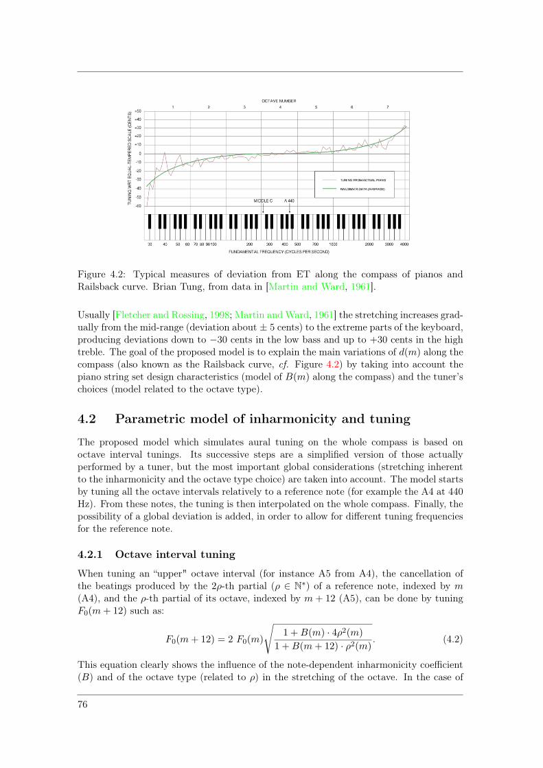
Figure 4.2: Typical measures of deviation from ET along the compass of pianos andRailsback curve. Brian Tung, from data in [Martin and Ward, 1961].
Usually [Fletcher and Rossing, 1998; Martin and Ward, 1961] the stretching increases grad-ually from the mid-range (deviation about ± 5 cents) to the extreme parts of the keyboard,producing deviations down to −30 cents in the low bass and up to +30 cents in the hightreble. The goal of the proposed model is to explain the main variations of d(m) along thecompass (also known as the Railsback curve, cf. Figure 4.2) by taking into account thepiano string set design characteristics (model of B(m) along the compass) and the tuner’schoices (model related to the octave type).
4.2 Parametric model of inharmonicity and tuning
The proposed model which simulates aural tuning on the whole compass is based onoctave interval tunings. Its successive steps are a simplified version of those actuallyperformed by a tuner, but the most important global considerations (stretching inherentto the inharmonicity and the octave type choice) are taken into account. The model startsby tuning all the octave intervals relatively to a reference note (for example the A4 at 440Hz). From these notes, the tuning is then interpolated on the whole compass. Finally, thepossibility of a global deviation is added, in order to allow for different tuning frequenciesfor the reference note.
4.2.1 Octave interval tuning
When tuning an “upper" octave interval (for instance A5 from A4), the cancellation ofthe beatings produced by the 2ρ-th partial (ρ ∈ N
∗) of a reference note, indexed by m(A4), and the ρ-th partial of its octave, indexed by m + 12 (A5), can be done by tuningF0(m+ 12) such as:
F0(m+ 12) = 2 F0(m)
√1 +B(m) · 4ρ2(m)
1 +B(m+ 12) · ρ2(m). (4.2)
This equation clearly shows the influence of the note-dependent inharmonicity coefficient(B) and of the octave type (related to ρ) in the stretching of the octave. In the case of
76

CHAPTER 4. A PARAMETRIC MODEL FOR THE INHARMONICITY AND TUNING ALONG THE WHOLE COMPASS
“lower" octave tuning (for instance A3 from A4), the same relation can be inverted andapplied by considering m+12 (A4) as the reference note and m (A3) as the note to tune.The next sections describe parametric models for B and ρ along the whole compass.
4.2.2 Whole compass model for the inharmonicity
4.2.2.1 String set design influence
In order to keep an homogeneous timbre along the compass, the strings are designed in sucha way that discontinuities due to physical parameters variations are smoothed [Conklin,Jr., 1996b; Engelbrecht et al., 1999; Stulov, 2008]. Three main design considerations mightproduce such discontinuities in B along the keyboard: the bass break between the bassand treble bridges (jump in L, the speaking length of the strings, cf. Figure 4.3), thetransitions between adjacent keys having a different number of strings (jump in T , thetension of each string [Engelbrecht et al., 1999; Fletcher and Rossing, 1998]), and thetransition between plain strings to wrapped strings (jump in d, the diameter of the pianowire [Engelbrecht et al., 1999]).
On the treble bridge, from C8 note downwards, B is decreasing because of the increaseof L. Down to middle C (C4 note, m = 60), the values of B are roughly the same for allthe pianos and B follows a straight line in logarithmic scale [Young, 1952]. This resultis mainly due to the fact that string design in this range is standardized, since it is notconstrained by the limitation of the piano size [Conklin, Jr., 1996b].
In the low pitch range, the strings use a different bridge (the bass bridge) to keepa reasonable size of the instrument. Then, the linear mass of the strings is increased inorder to adjust the value of F0 according to Equation (2.21). Instead of increasing only thediameter d, which increases B (cf. Equation (2.24)), the strings are wound with a copperstring wire, which increases the linear mass. Thus, on the bass bridge, B is increasing fromsharpest notes downwards. Note that the number of keys associated to the bass bridgeand the design of their strings are specific to each piano.
Figure 4.3: Grand piano string and bridge design. From [Conklin, Jr., 1996b].
77

4.2.2.2 Parametric model
According to the string design considerations, B could be modeled by two distinct func-tions corresponding to the two bridges, and could present discontinuities at the bass breakor at the changes single-doublets and doublets-triplets of strings. The difficulty whenmodeling B on the whole compass is to know the position of these possible discontinuities,because they are specific to each piano model. Therefore, we propose a “continuous” ad-ditive model on the whole compass, discretized for m ∈ [21, 108]. We denote it by Bξ(m),ξ being the set of modeling parameters.
Usually, the evolution of B along the keyboard is depicted in logarithmic scale andpresents two linear asymptotes. We denote by bT (m) (resp. bB(m)) the treble bridge(resp. the bass bridge) asymptote of logBξ(m). Each asymptote is parametrized by itsslope and its Y-intercept:
bT (m) = sT ·m+ yT ,
bB(m) = sB ·m+ yB.(4.3)
According to Young et al. [Young, 1952], bT (m) is similar for all the pianos so sT andyT are fixed parameters. Then, the set of free (piano dependent) parameters reduces toξ = sB, yB. Bξ(m) is set as the sum of the contributions of these two curves (4.3) inthe linear scale:
Bξ(m) = ebB(m) + ebT (m) (4.4)
It should be emphasized that this additivity does not arise from physical considerations,but it is the simplest model that smoothes discontinuities between the bridges. Experi-mental data will show that it actually describes well the variations of B in the transitionregion around the two bridges.
The model is presented on Figure 4.4(a) for three different typical values of the set ofparameters: ξ1, ξ2 and ξ3, corresponding to low, medium and highly inharmonic pianos,respectively. The asymptotes corresponding to the bass and treble bridges are also drawnfor Bξ2(m).
4.2.3 Whole compass model for the octave type parameter
The octave tuning relation, given in Equation (4.2), considers the cancellation of the
beatings produced by a single pair of partials. In practice, the deviation F0(m+12)2F0(m) could
be a weighted sum of the contribution of two pairs of partials, because the amount ofstretching may result from a compromise between two octave types [Bremmer, 2007a].An alternative model to take into account this weighting is to allow non-integer values forρ ∈ [1,+∞[. For example, if the octave tuning is a compromise between a 2:1 and 4:2 typeoctaves, ρ will be in the interval [1, 2]. This model loses the physical meaning because ρis not anymore related to a partial rank ; it will however be shown in Section 4.3 that itallows the inversion of Equation (4.2), in order to estimate ρ from the data.
We choose arbitrarily to model the evolution of ρ along the compass as follows:
ρφ(m) =κ
2·(1− erf
(m−m0
α
))+ 1, (4.5)
with erf the error function, and φ = κ,m0, α the set of parameters. Note that ρφ isindexed by the note m, and not by the note m + 12 (cf. Equation (4.2)). It is then
78

CHAPTER 4. A PARAMETRIC MODEL FOR THE INHARMONICITY AND TUNING ALONG THE WHOLE COMPASS
defined for m ∈ [21, 96]. κ is related to the value of the asymptote in the low bass range.m0 is a parameter of translation along m and α rules the slope of the decrease. Thismodel expresses the fact that the amount of stretching inherent to the octave type choiceis decreasing from the low bass to the high treble range.
It may be justified by the fact that the perception of the pitch of complex tones isnot only based on the first partial of the notes, but on a set of partials contained in a“dominant region” of the human hearing [Moore et al., 1984; Ritsma, 1967; Plomp, 1967].For bass tones (with fundamental frequencies around 100 to 400 Hz, i.e. in the range G2-G4, m ∈ [43, 67]), this dominant region covers the third to fifth partials [Ritsma, 1967].While going up to the treble part of the compass, the dominant region tends to be localizedon the partials with a lower rank. For tones having a first partial frequency above 1400 Hz(i.e. for a higher note than F6, m = 89) the perception of the pitch is mainly linked to thefirst partial [Plomp, 1967]. Further research on the pitch perception of inharmonic tonesconsistently shown that the pitch perception is based on one dominant partial whose rankis decreasing from the bass (6 for A1) to the treble range (2 for C♯6) [Järveläinen et al.,2002]. Moreover, the perceived pitch frequency has been found equal to the frequency ofthe dominant partial divided by its rank (such as the sixth partial frequency divided bysix for the A1). In accordance with those studies, in the presented octave type model thehigh treble asymptote is set to 1. It corresponds to the minimal octave type (2:1), andmeans that the tuner focuses on the first partial of the highest note. In the low bass range,the asymptote is set by the value of the parameter κ+ 1.
The model is represented on Figure 4.4(b) for three different values of the set ofparameters: φ1, φ2 and φ3, respectively corresponding to a low, mid and high octave typechoice in the low bass range.
4.2.4 Interpolation of the tuning along the whole compass
From the estimation of the sets of parameters, ξ related to the design of the strings, andφ related to the choices of the tuner, it is possible to tune all the octaves of a referencenote. If A4 is tuned such that f1(m = 69) = 440 Hz, all the A notes of the keyboardcan be iteratively tuned by using Equation (4.2). To complete the tuning on the wholecompass, a Lagrange polynomial interpolation is performed on the deviation from ET ofthe tuned notes of the model (computed by using Equation (4.1)). The interest of thismethod is that the interpolated curve is constrained to coincide with the initial data. Theinterpolated model of deviation from ET is denoted by dξ,φ(m).
4.2.5 Global deviation
Finally, in order to take into account the fact that the reference note is not necessarilya A4 at 440 Hz (other tuning forks exist, for instance A4 at 442 Hz or C5 at 523.3 Hz)we add in the model the possibility of a global “detuning”. In the representation of thedeviation from ET in cents, it corresponds to a vertical translation of the curve. Then,the deviation from ET of the model is set to dξ,φ(m)+ dg, where dg is an extra parameterof the model, corresponding to the global deviation.
The whole compass tuning model is depicted on Figure 4.5 for different values of thesets of parameters ξ and φ (corresponding to those used in Figure 4.4), and for dg = 0.The tuning of the A notes from A4 at 440 Hz is indicated with black dots on the middlecurves. Sub-figure 4.5(a) corresponds to the influence on the tuning of Bξ (for ξ1, ξ2 and
79

20 30 40 50 60 70 80 90 100 110
10−4
10−3
10−2
m (note in MIDI index)
Bξ (
log
sca
le)
ξ1
ξ2
ξ3
Bξ1
Bξ2
treble bridge asymptote bT2
(m)
bass bridge asymptote bB2
(m)
Bξ3
(a)
20 30 40 50 60 70 80 90 100 1100
1
2
3
4
5
6
m (note in MIDI index)
ρφ
φ1
φ2
φ3
2:1
4:2
6:3
8:4
10:5Octave type
(b)
Figure 4.4: Model for (a) the inharmonicity coefficient Bξ(m) and (b) octave type param-eter ρφ(m) along the compass for different values of the sets of parameters.
20 30 40 50 60 70 80 90 100 110−15
−10
−5
0
5
10
15
20
25
30
35
m (note in MIDI index)
dξ,
φ
(in
ce
nts
)
ξ1
ξ2
ξ3
for φ2
A4 (440 Hz) reference note
(a)
20 30 40 50 60 70 80 90 100 110−20
−10
0
10
20
30
40
m (note in MIDI index)
dξ,
φ
(in
ce
nts
)
φ1
φ2
φ3
for ξ2
A4 (440 Hz) reference note
(b)
Figure 4.5: Model for the deviation of tuning from ET along the compass. (a) Influenceof ξ in the tuning for φ fixed. (b) Influence of φ in the tuning for ξ fixed. The differentvalues for ξ and φ correspond to those used to generate the curves of Figure 4.4.
80
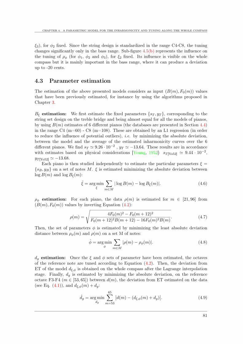
CHAPTER 4. A PARAMETRIC MODEL FOR THE INHARMONICITY AND TUNING ALONG THE WHOLE COMPASS
ξ3), for φ2 fixed. Since the string design is standardized in the range C4-C8, the tuningchanges significantly only in the bass range. Sub-figure 4.5(b) represents the influence onthe tuning of ρφ (for φ1, φ2 and φ3), for ξ2 fixed. Its influence is visible on the wholecompass but it is mainly important in the bass range, where it can produce a deviationup to -20 cents.
4.3 Parameter estimation
The estimation of the above presented models considers as input (B(m), F0(m)) valuesthat have been previously estimated, for instance by using the algorithms proposed inChapter 3.
Bξ estimation: We first estimate the fixed parameters sT , yT , corresponding to thestring set design on the treble bridge and being almost equal for all the models of pianos,by using B(m) estimates of 6 different pianos (the databases are presented in Section 4.4)in the range C4 (m=60) - C8 (m=108). These are obtained by an L1 regression (in orderto reduce the influence of potential outliers), i.e. by minimizing the absolute deviation,between the model and the average of the estimated inharmonicity curves over the 6different pianos. We find sT ≃ 9.26 · 10−2 , yT ≃ −13.64. These results are in accordancewith estimates based on physical considerations [Young, 1952]: sT [Yo52] ≃ 9.44 · 10−2,yT [Yo52] ≃ −13.68.
Each piano is then studied independently to estimate the particular parameters ξ =sB, yB on a set of notes M . ξ is estimated minimizing the absolute deviation betweenlogB(m) and logBξ(m):
ξ = argminξ
∑
m∈M| logB(m)− logBξ(m)|. (4.6)
ρφ estimation: For each piano, the data ρ(m) is estimated for m ∈ [21, 96] from(B(m), F0(m)) values by inverting Equation (4.2):
ρ(m) =
√4F0(m)2 − F0(m+ 12)2
F0(m+ 12)2B(m+ 12)− 16F0(m)2B(m). (4.7)
Then, the set of parameters φ is estimated by minimizing the least absolute deviationdistance between ρφ(m) and ρ(m) on a set M of notes:
φ = argminφ
∑
m∈M|ρ(m)− ρφ(m)|. (4.8)
dg estimation: Once the ξ and φ sets of parameter have been estimated, the octavesof the reference note are tuned according to Equation (4.2). Then, the deviation fromET of the model dξ,φ is obtained on the whole compass after the Lagrange interpolationstage. Finally, dg is estimated by minimizing the absolute deviation, on the referenceoctave F3-F4 (m ∈ [53, 65]) between d(m), the deviation from ET estimated on the data(see Eq. (4.1)), and dξ,φ(m) + dg:
dg = argmindg
65∑
m=53
∣∣d(m)− (dξ,φ(m) + dg)∣∣. (4.9)
81

4.4 Applications
The results presented in this section are obtained from 6 different pianos (the Iowa andthe 3 RWC grand pianos, and the MAPS ENSTDkCl upright piano and SptkBGCl grandpiano synthesizer) of the database presented in Section 3.1.3.1, page 48. The estimatesof (B,F0) are obtained by using InhR-NMF algorithm on isolated note recordings in asupervised way (cf. Section 3.1).
4.4.1 Modeling the tuning of well-tuned pianos
The results of the estimation of the whole compass tuning model for four different pianosare presented on Figures 4.6 (RWC3), 4.7 (RWC2), 4.8 (Iowa) and 4.9 (MAPS SptkBGCl).Sub-figures (a), (b) and (c), correspond to the inharmonicity coefficient B, the octave typeparameter ρ and the deviation from ET curves along the whole compass, respectively. Thedata corresponding to the estimation of (B,F0) from isolated note recordings is depictedas ‘+’ markers, and the model as black lines. The values of the parameters for each pianoare given in Table 4.1.
B along the compass (sub-figures (a)): The estimation of the parameters has beenperformed from a limited set of 4 notes (black dot markers), taken in the bass range andequally spaced by fifth intervals. As the string set design on each bridge is quite regular,a few notes can be used to correctly estimate the model. In the case where an importantdiscontinuity is present in the variations of B(m) (for instance between C2 (m = 37) andD2 (m = 38) notes, on Figure 4.7(a)) the 2-bridges additive model produces a smoothcurve. It is worth noting from RWC2 grand piano design characteristics that the slightjump between D♯1 (m = 27) and E1 (m = 28) might be explained by the single stringto doublet of strings transition, and the important jump between C2 (m = 37) and D2(m = 38) by the bridge change, jointly with the transition from doublet of strings totriplet.
ρ along the compass (sub-figures (b)): The curves of ρ(m) can present a significantdispersion around the mean model ρφ(m), but the global variations are well reproduced.In the medium range, the estimated octave types are a trade-off between 6:3 and 4:2,which is common in piano tuning [Bremmer, 2007a]. The variations, more important inthe bass range, could be explained by the fact that the model of the partial frequencies(cf. Equation (2.23)) does not take into account the frequency shifts caused by the bridgecoupling, mainly appearing in the low frequency domain. Moreover, the proposed tuningmodel is a simplification of a real tuning procedure, it is based on octave interval tuning,while an expert tuner would jointly control different intervals along the keyboard and cando local readjustments after a global tuning. Note that some values of ρ(m) can be missingwhen the quantity under the square root of Equation (4.7) is negative. This happens ifthe corresponding octave interval is compressed instead of being stretched.
Deviation from ET along the compass (sub-figures (c)): The curves demonstratethat the model reproduces the main variations of the tuning in a satisfactory manner.This confirms that, besides the well-known influence of the inharmonicity on the tuning,perceptual effects (taken into account through the octave type consideration) can take partin the stretching, mainly in the bass range. Note that the tuning of A notes is markedwith black dot markers.
82

CHAPTER 4. A PARAMETRIC MODEL FOR THE INHARMONICITY AND TUNING ALONG THE WHOLE COMPASS
20 30 40 50 60 70 80 90 100 110
104
103
102
m (note in MIDI index)
B (
log
sca
le)
reference data: B(m), m [21:108]
data used for the estimation of the model: B(m), m Mmodel B (m)
(a)
20 30 40 50 60 70 80 90 100 1100
1
2
3
4
5
6
7
8
m (note in MIDI index)
2:1
4:2
6:3
8:4
10:5
Octave type
data (m), m [21,96]model (m)
(b)
20 30 40 50 60 70 80 90 100 11010
0
10
20
30
40
m (note in MIDI index)
d (
in c
en
ts)
reference data d(m)
tuning of A notesmodel d
,(m)+d
g
(c)
Figure 4.6: RWC3 grand piano. (a) Inharmonicity coefficient B, (b) octave type parameterρ, (c) deviation from ET along the whole compass. The data are depicted as gray ‘+’markers and the model as black lines.
83

20 30 40 50 60 70 80 90 100 110
104
103
102
m (note in MIDI index)
B (
log
sca
le)
reference data: B(m), m [21:108]
data used for the estimation of the model: B(m), m Mmodel B (m)
(a)
20 30 40 50 60 70 80 90 100 1100
1
2
3
4
5
6
7
8
m (note in MIDI index)
2:1
4:2
6:3
8:4
10:5
Octave type
data (m), m [21,96]model (m)
(b)
20 30 40 50 60 70 80 90 100 110
10
0
10
20
30
40
m (note in MIDI index)
d (
in c
en
ts)
reference data d(m)
tuning of A notesmodel d
,(m)+d
g
(c)
Figure 4.7: RWC2 grand piano. (a) Inharmonicity coefficient B, (b) octave type parameterρ, (c) deviation from ET along the whole compass. The data are depicted as gray ‘+’markers and the model as black lines.
84

CHAPTER 4. A PARAMETRIC MODEL FOR THE INHARMONICITY AND TUNING ALONG THE WHOLE COMPASS
20 30 40 50 60 70 80 90 100 110
104
103
102
m (note in MIDI index)
B (
log
sca
le)
Iow mf
reference data: B(m), m [21:108]
data used for the estimation of the model: B(m), m Mmodel B (m)
(a)
20 30 40 50 60 70 80 90 100 1100
1
2
3
4
5
6
7
m (note in MIDI index)
2:1
4:2
6:3
8:4
10:5
Octave typedata (m), m [21,96]model (m)
(b)
20 30 40 50 60 70 80 90 100 110
20
10
0
10
20
30
40
m (note in MIDI index)
d (
in c
en
ts)
reference data d(m)
tuning of A notesmodel d
,(m)+d
g
(c)
Figure 4.8: Iowa grand piano. (a) Inharmonicity coefficient B, (b) octave type parameterρ, (c) deviation from ET along the whole compass. The data are depicted as gray ‘+’markers and the model as black lines.
85

20 30 40 50 60 70 80 90 100 110
104
103
102
m (note in MIDI index)
B (
log
sca
le)
reference data: B(m), m [21:108]
data used for the estimation of the model: B(m), m Mmodel B (m)
(a)
20 30 40 50 60 70 80 90 100 1100
1
2
3
4
5
6
7
m (note in MIDI index)
2:1
4:2
6:3
8:4
10:5
Octave typedata (m), m [21,96]model (m)
(b)
20 30 40 50 60 70 80 90 100 11010
0
10
20
30
40
m (note in MIDI index)
d (
in c
en
ts)
reference data d(m)
tuning of A notesmodel d
,(m)+d
g
(c)
Figure 4.9: MAPS SptkBGCl. (a) Inharmonicity coefficient B, (b) octave type parameterρ, (c) deviation from ET along the whole compass. The data are depicted as gray ‘+’markers and the model as black lines.
86
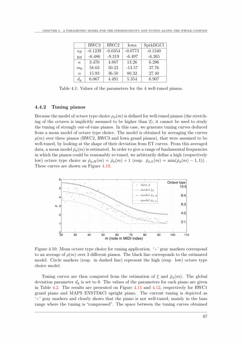
CHAPTER 4. A PARAMETRIC MODEL FOR THE INHARMONICITY AND TUNING ALONG THE WHOLE COMPASS
RWC3 RWC2 Iowa SptkBGCl
sB -0.1239 -0.0354 -0.0773 -0.1340yB -6.486 -9.319 -6.497 -6.265
κ 3.470 4.887 13.26 6.296m0 58.03 50.22 -13.57 37.76α 15.93 36.50 80.32 27.40
dg 6.067 4.491 5.354 6.907
Table 4.1: Values of the parameters for the 4 well-tuned pianos.
4.4.2 Tuning pianos
Because the model of octave type choice ρφ(m) is defined for well-tuned pianos (the stretch-ing of the octaves is implicitly assumed to be higher than 2), it cannot be used to studythe tuning of strongly out-of-tune pianos. In this case, we generate tuning curves deducedfrom a mean model of octave type choice. The model is obtained by averaging the curvesρ(m) over three pianos (RWC2, RWC3 and Iowa grand pianos), that were assumed to bewell-tuned, by looking at the shape of their deviation from ET curves. From this averageddata, a mean model ρφ(m) is estimated. In order to give a range of fundamental frequenciesin which the pianos could be reasonably re-tuned, we arbitrarily define a high (respectivelylow) octave type choice as ρφ,H(m) = ρφ(m) + 1 (resp. ρφ,L(m) = min(ρφ(m) − 1, 1)) .These curves are shown on Figure 4.10.
20 30 40 50 60 70 80 90 100 1100
1
2
3
4
5
6
m (note in MIDI index)
2:1
4:2
6:3
8:4
10:5
Octave typedata ρ
model ρφ
model ρφ,H
model ρφ,L
Figure 4.10: Mean octave type choice for tuning application. ‘+’ gray markers correspondto an average of ρ(m) over 3 different pianos. The black line corresponds to the estimatedmodel. Circle markers (resp. in dashed line) represent the high (resp. low) octave typechoice model.
Tuning curves are then computed from the estimation of ξ and ρφ(m). The globaldeviation parameter dg is set to 0. The values of the parameters for each piano are givenin Table 4.2. The results are presented on Figure 4.11 and 4.12, respectively for RWC1grand piano and MAPS ENSTDkCl upright piano. The current tuning is depicted as‘+’ gray markers and clearly shows that the piano is not well-tuned, mainly in the bassrange where the tuning is “compressed”. The space between the tuning curves obtained
87
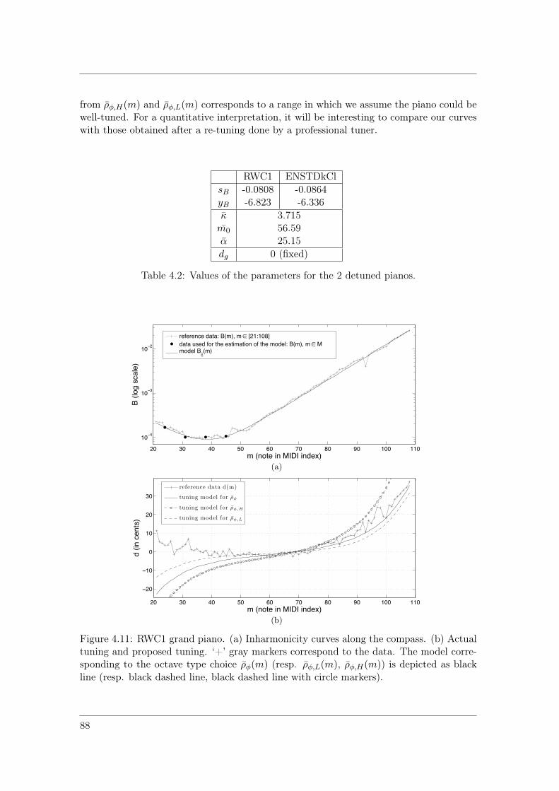
from ρφ,H(m) and ρφ,L(m) corresponds to a range in which we assume the piano could bewell-tuned. For a quantitative interpretation, it will be interesting to compare our curveswith those obtained after a re-tuning done by a professional tuner.
RWC1 ENSTDkCl
sB -0.0808 -0.0864yB -6.823 -6.336
κ 3.715m0 56.59α 25.15
dg 0 (fixed)
Table 4.2: Values of the parameters for the 2 detuned pianos.
20 30 40 50 60 70 80 90 100 110
104
103
102
m (note in MIDI index)
B (
log s
cale
)
reference data: B(m), m [21:108]
data used for the estimation of the model: B(m), m Mmodel B (m)
(a)
20 30 40 50 60 70 80 90 100 110
20
10
0
10
20
30
m (note in MIDI index)
d (
in c
ents
)
reference data d(m)
tuning model for ρφ
tuning model for ρφ,H
tuning model for ρφ,L
(b)
Figure 4.11: RWC1 grand piano. (a) Inharmonicity curves along the compass. (b) Actualtuning and proposed tuning. ‘+’ gray markers correspond to the data. The model corre-sponding to the octave type choice ρφ(m) (resp. ρφ,L(m), ρφ,H(m)) is depicted as blackline (resp. black dashed line, black dashed line with circle markers).
88

CHAPTER 4. A PARAMETRIC MODEL FOR THE INHARMONICITY AND TUNING ALONG THE WHOLE COMPASS
20 30 40 50 60 70 80 90 100 110
104
103
102
m (note in MIDI index)
B (
log s
cale
)
reference data: B(m), m [21:108]
data used for the estimation of the model: B(m), m Mmodel B (m)
(a)
20 30 40 50 60 70 80 90 100 110
30
20
10
0
10
20
30
40
m (note in MIDI index)
d (
in c
ents
)
reference data d(m)
tuning model for ρφ
tuning model for ρφ,H
tuning model for ρφ,L
(b)
Figure 4.12: MAPS ENSTDkCl upright piano. (a) Inharmonicity curves along the com-pass. (b) Actual tuning and proposed tuning. ‘+’ gray markers correspond to the data.The model corresponding to the octave type choice ρφ(m) (resp. ρφ,L(m), ρφ,H(m)) isdepicted as black line (resp. black dashed line, black dashed line with circle markers).
4.4.3 Initializing algorithms
As show in Chapter 3, a good initialization of (B,F0) parameters in analysis algorithmsis a matter of importance in order to avoid the convergence of the algorithms towardlocal optima. The curves for the initialization of these parameters are here obtained byconsidering a mean model, obtained from the 6 pianos analyzed in this chapter. Theseare presented on Figure 4.13. Subplot 4.13(a) depicts in black line the initialization curveBini, estimated from the data averaged over the 6 pianos (‘+’ markers). The low andhigh limit curves (respectively denoted by BL
lim and BHlim) used in Section 3.2.2.3 for the
PLS algorithm are obtained by means of a manual tuning of ξ so that all estimates arecontained in the delimited area (values given in Table 4.3). Then, the initialization curveof F0 is computed from Bini and ρφ, the mean octave type obtained in the previous section.
Bini BLlim BH
lim
sB -0.0889 -0.047 -0.083yB -7.0 -9.5 -6.0
Table 4.3: Values of the parameters for the initialization and limit curves of B.
89

20 30 40 50 60 70 80 90 100 110
10−4
10−3
10−2
m (note in MIDI index)
B (
log
sca
le)
Bini
Blim
H
Blim
L
data from 6 pianos
(a)
20 30 40 50 60 70 80 90 100 110
−15
−10
−5
0
5
10
15
m (note in MIDI index)
F0/F
0,E
T (
ce
nts
)
(b)
Figure 4.13: Mean model for the initialization of (B,F0) in piano analysis algorithms. (a)‘+’ markers correspond to the values of B for the 6 different pianos. In black line, Bini,the model estimated from the estimates averaged over the 6 pianos. In dashed lines, thelimit curves for B values. (b) Mean model for F0 computed from Bini and ρφ.
4.4.4 Learning the tuning on the whole compass from the analysis of a
piece of music
Finally, the whole compass model is applied to the interpolation of (B,F0) estimates ob-tained on a restricted set of notes from the analysis of a piece of music. The results aredepicted in Figure 4.14 for the example presented in Section 3.2.3.2. The input data ishere depicted as ‘+’ red markers and the interpolated curves are plotted as black lines.The gray curve, displayed for comparison purposes, corresponds to the estimates alongthe whole compass obtained by the PLS algorithm from isolated notes processed in asupervised way (the algorithm knows which notes are being played). When comparing theinterpolated model and the reference curve, one can see that the main trends are fairlywell reproduced. Averaged below note C♯7 (97) (i.e. for the range where the referencedata is reliable, as discussed in Section 3.2.3.1), a mean relative error of 9.48 % is obtainedfor B and a mean deviation of 2.20 cents for F0.
It is worth noting that a few requirements are needed for this interpolation application.First, since the variations of B between different pianos are mainly present for the notes
90

CHAPTER 4. A PARAMETRIC MODEL FOR THE INHARMONICITY AND TUNING ALONG THE WHOLE COMPASS
associated to the bass bridge, the interpolation requires estimates in the bass range. Onecan see on Figure 4.14(a), that 4 notes were present below note E2 (40) in the input data.Here, one can assume that the interpolation may have been improved with a few moreestimates below note E1 (28). Second, since the tuning model, given in Equation (4.2), isbased on the tuning of octave intervals, the input data has to contain, as much as possible,(B,F0) estimates for octave-related notes. In the presented example, 6 octave intervalswere present. Thus, in order to increase the number of input data, that should lead to ahigher precision of the interpolation, one could consider processing several pieces of musicplayed by the same instrument.
20 30 40 50 60 70 80 90 100
10−4
10−3
10−2
note (in MIDI index)
B (
log. scale
)
PLS reference
PLS unsupervised est.
WC interpolation
(a)
20 30 40 50 60 70 80 90 100−15
−10
−5
0
5
10
15
20
m (note in MIDI index)
F0 / F
0,E
T (
in c
ents
)
PLS reference
PLS unsupervised est.
WC interpolation
(b)
Figure 4.14: (B,F0) interpolation along the whole compass from a few estimates obtainedon a piece of music with PLS algorithm (cf. Section 3.2.3.2). (a) B in log. scale and(b) F0 as dev. from ET in cents. The whole compass models (black lines, denoted as“WC interpolation”) are estimated from the data obtained by the unsupervised analysisof a piece of music (red markers). These are compared with the reference curves (graymarkers) obtained from the supervised analysis on isolated note recordings.
91

92

Chapter 5
Application to the transcription ofpolyphonic piano music
This chapter presents the evaluation on a transcription task of the two inharmonic NMF-based models introduced in Chapter 3. In order to quantify the benefits or losses that mayresult from the inclusion of the inharmonicity, the performances are compared with thoseobtained by a simpler harmonic model. Influence of the model design, the initializationand the optimization are then investigated. Portions of this work have been published in[Rigaud et al., 2013c].
5.1 Automatic polyphonic music transcription
This section introduces briefly the music transcription task, and defines the metrics com-monly used when assessing the performance of the methods. For a complete descriptionand an exhaustive state of the art of this domain, the interested reader may refer to[Klapuri and Davy, 2006; Emiya, 2008; Bertin, 2009; Benetos, 2012].
5.1.1 The task
Automatic music transcription is the process of recovering a symbolic representation of amusical piece, such as for instance a score, a chord grid or a guitar tablature, from theunsupervised analysis of a performance recording. According to the degree of informationwhich is targeted, the problem is usually decomposed into several sub-tasks, each focusingon the extraction of a specific feature related to the musical structure. These can be forinstance the recovery of the played notes (their pitch, loudness, onset time and duration),but also higher-level information, such as the instruments, the rhythmic structure (e.g.tempo and time signature), the tonality, or the detection of musical sequence repetitions.
Automatic music transcription, and more generally tasks related to Music InformationRetrieval, have become a very active field of research this last decade due to their widerange of applications. Beyond straightforward uses as supports for musical practice ormusicological analysis, applications include automatic music data indexing for classifica-tion/search purposes. Also, when processed in real-time during a musical performance,the extracted information can be used as control inputs in human-machine interactivesystems (e.g. score following or rhythm tracking for automatic accompaniment).
93

In the case of the analysis of a Western tonal piece of music, the most completetranscription task corresponds to the retrieval of the score. However as mentioned above,this complex representation requires the processing of a large number of sub-tasks. Thus,in this thesis as in most works related to music transcription using NMF-based models,we restrict the transcription problem to the detection of the notes (pitch) that are played,jointly with their onset and duration. Thus the obtained representation is usually displayedin the form of a piano roll (i.e. binary activation of the notes according to the time axis,as shown in Figure 5.1).
As seen in Chapter 2, NMF-based methods seem particularly relevant for the task ofaudio to piano roll transcription as the activation matrix H naturally presents a structuresimilar to the desired representation. However, a binary decision (note active/inactive)along the lines of H is required after the NMF optimization. Such post-processing mayinclude additional temporal modeling of notes, based for instance on Hidden MarkovModels [Poliner and Ellis, 2007; Emiya et al., 2010a], or heuristics based on thresholdingand gathering of adjacent activated frames [Vincent et al., 2010; Dessein et al., 2010].
Time (s)
Note
s (
in M
IDI in
dex)
0 0.5 1 1.5 2 2.5 3 3.550
55
60
65
70
75
80
85
Figure 5.1: Piano roll of the first bar of the score given in Figure 2.1.
5.1.2 Performance evaluation
The performance evaluation of transcription algorithms requires a ground truth, for in-stance in the form of a synchronized MIDI file. Such reference may be obtained after amanual annotation of the data (as for the RWC database), or by synthesizing the mu-sic signals directly from the MIDI reference file. This latter case presents the advantageof ensuring the near-perfect alignment between the audio and the ground truth and ofavoiding errors inherent in the manual annotation process. This is the case for the MAPSdatabase used for our experiments, and for which the generation of the audio is usingeither piano synthesizers based on high quality sampling, or a MIDI controlled acousticpiano (cf. details in Section 3.1.3.1).
Thus, when evaluating the performance, each note detected by the algorithm can beclassified into two classes. If the note is actually present in the ground truth, it is labeledas True Positive (TP). If not, it corresponds to a false detection and it is labeled as FalsePositive (FP). Finally, the notes that are missing (i.e. not detected by the algorithm,although present in the ground truth) are labeled as False Negative (FN). These classes,common in classification task evaluations, are summarized in Table 5.1. Note that a fourthcategory True Negative (TN) exists but it is not used in a transcription context since itis not relevant. Indeed, it corresponds to a non-detection when the note is not present inthe ground truth.
94
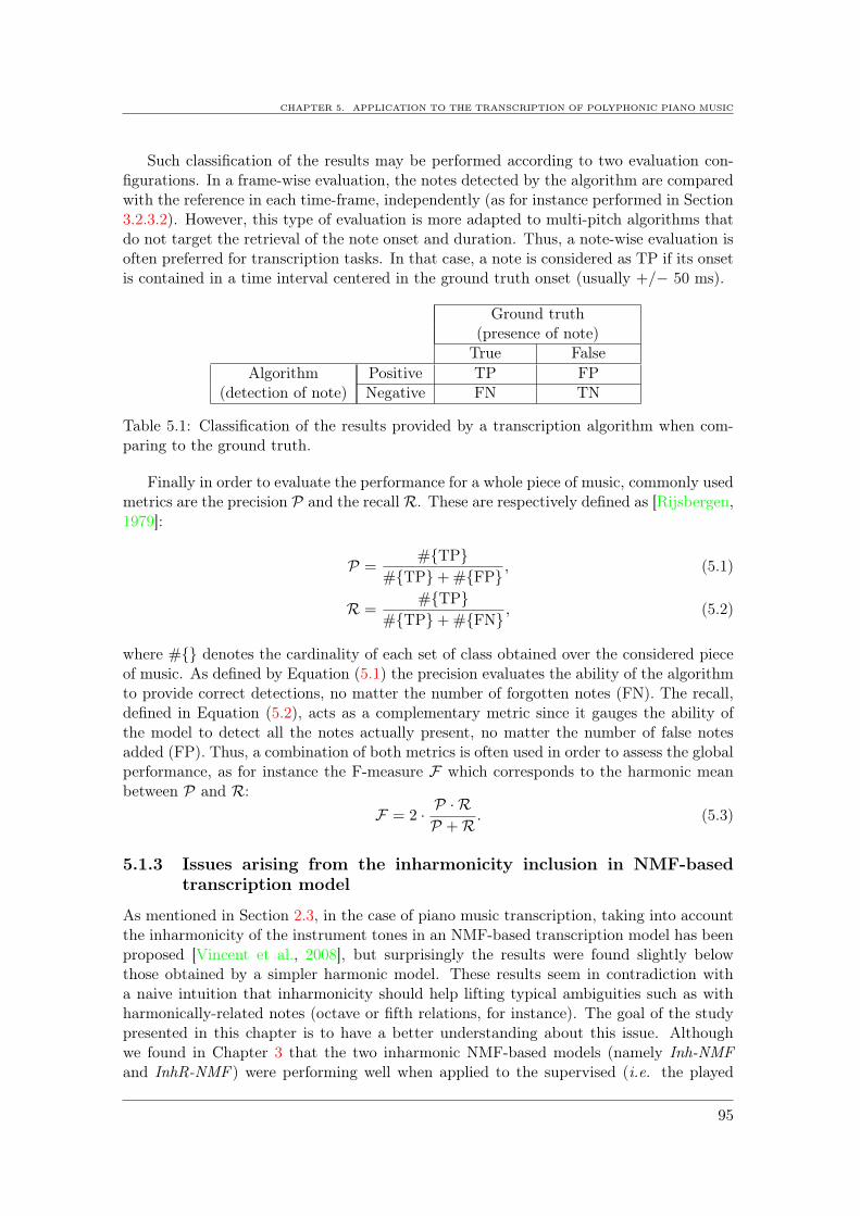
CHAPTER 5. APPLICATION TO THE TRANSCRIPTION OF POLYPHONIC PIANO MUSIC
Such classification of the results may be performed according to two evaluation con-figurations. In a frame-wise evaluation, the notes detected by the algorithm are comparedwith the reference in each time-frame, independently (as for instance performed in Section3.2.3.2). However, this type of evaluation is more adapted to multi-pitch algorithms thatdo not target the retrieval of the note onset and duration. Thus, a note-wise evaluation isoften preferred for transcription tasks. In that case, a note is considered as TP if its onsetis contained in a time interval centered in the ground truth onset (usually +/− 50 ms).
Ground truth(presence of note)
True False
Algorithm Positive TP FP(detection of note) Negative FN TN
Table 5.1: Classification of the results provided by a transcription algorithm when com-paring to the ground truth.
Finally in order to evaluate the performance for a whole piece of music, commonly usedmetrics are the precision P and the recall R. These are respectively defined as [Rijsbergen,1979]:
P =#TP
#TP+#FP , (5.1)
R =#TP
#TP+#FN , (5.2)
where # denotes the cardinality of each set of class obtained over the considered pieceof music. As defined by Equation (5.1) the precision evaluates the ability of the algorithmto provide correct detections, no matter the number of forgotten notes (FN). The recall,defined in Equation (5.2), acts as a complementary metric since it gauges the ability ofthe model to detect all the notes actually present, no matter the number of false notesadded (FP). Thus, a combination of both metrics is often used in order to assess the globalperformance, as for instance the F-measure F which corresponds to the harmonic meanbetween P and R:
F = 2 · P · RP +R . (5.3)
5.1.3 Issues arising from the inharmonicity inclusion in NMF-based
transcription model
As mentioned in Section 2.3, in the case of piano music transcription, taking into accountthe inharmonicity of the instrument tones in an NMF-based transcription model has beenproposed [Vincent et al., 2008], but surprisingly the results were found slightly belowthose obtained by a simpler harmonic model. These results seem in contradiction witha naive intuition that inharmonicity should help lifting typical ambiguities such as withharmonically-related notes (octave or fifth relations, for instance). The goal of the studypresented in this chapter is to have a better understanding about this issue. Althoughwe found in Chapter 3 that the two inharmonic NMF-based models (namely Inh-NMFand InhR-NMF ) were performing well when applied to the supervised (i.e. the played
95

notes were known) estimation of (B,F0), it is not straightforward that such models mayprovide good results in the context of unsupervised analysis, i.e. when the matrix H hasto be estimated jointly with the inharmonicity relation parameters. Since it is difficultto gauge intrinsically the quality of NMF decompositions, these are here evaluated on atranscription task, on a large database of piano recordings from MAPS where we have aground-truth transcription at hand. Performances of both inharmonic models are eval-uated and compared with a similar parametric harmonic model. Influence of the modeldesign (harmonicity vs. inharmonicity and number of partials considered), of the initial-ization (naive initialization vs. mean model of inharmonicity and tuning along the wholecompass) and of the optimization process (number of partials fixed at the initializationvs. iterative inclusion) are then investigated. The parameter of the β-divergence used todefine the reconstruction cost-function is here fixed to β = 1 (KL divergence).
It should be emphasized that the proposed algorithms do not target to be compet-itive with state-of-the-art fully dedicated piano transcription algorithms, since the onlyinformation that is taken into account is the inharmonicity of piano tones (for instance, nomodel of smooth spectral envelope or temporal continuity of the activations is considered).Here, the use of a simple threshold-based post-processing of H should allow one to betterhighlight the differences in the core model.
5.2 Does inharmonicity improve an NMF-based piano tran-
scription model?
5.2.1 Experimental setup
5.2.1.1 Database
The dataset consists of 45 pieces from MAPS database (cf. details of the pianos in Section3.1.3.1), randomly chosen (5 out of 30 for each of the 9 pianos) and re-sampled to 22050 Hz.For each piece, 30 second excerpts are taken, starting from t0 = 5 s. The mean polyphonylevel by time-frame is about 3.23. Then, the magnitude spectrograms are computed witha Hann window of length τ = 90 ms, a hop-size of τ/8 and a 213-point Fast FourierTransform.
The number of spectra in the dictionary is fixed to R = 64, and initialized for noteshaving MIDI note number in [33, 96] (A1 to C7). This choice corresponds to a reduction ofone octave in the extreme bass (where the spectral resolution is not sufficient to perform theanalysis) and one octave in the high treble range (where, as highlighted in Section 3.1.3.2,the non-linear coupling between triplets of strings at the soundboard produces complexspectra with multiple partials that cannot be fully explained by a simple harmonic orinharmonic model). However, these notes in the extreme parts of the keyboard are rarelyplayed. Over the complete MAPS dataset (352710 notes for 159 different pieces), theyonly account for 1.66% of the notes (cf. distribution of notes for the whole MAPS databaseon Figure 5.2).
5.2.1.2 Harmonicity vs. Inharmonicity
In order to quantify the benefits that may results from the inharmonicity inclusion inNMF-based model, the transcription performances are compared with a simpler harmonicmodel (thereafter denoted by Ha-NMF ) based on a similar parametric additive model of
96

CHAPTER 5. APPLICATION TO THE TRANSCRIPTION OF POLYPHONIC PIANO MUSIC
20 30 40 50 60 70 80 90 100 1100
0.005
0.01
0.015
0.02
0.025
0.03
0.035
Note (in MIDI index)
His
togra
m (
norm
aliz
ed)
Figure 5.2: Normalized histogram of note occurrences for the complete MAPS database.Black bars corresponds to the notes that are not considered in the analysis.
spectrum (cf. Equation (3.1), page 38).
• Strictly harmonic / Ha-NMF :We enforce harmonicity of the spectra of the dictionary by fixing
fnr = nF0r, n ∈ N∗, (5.4)
directly in the parametric model (Equation (3.1)). Then, the set of parameters for asingle atom corresponds to θHa
r = anr, F0r | n ∈ [1, Nr]. Similarly to Inh-NMF, thecost-function is defined as:
CHa(θHa, H) =∑
k∈K
T∑
t=1
dβ
(Vkt |
R∑
r=1
WθHar
kr ·Hrt
), (5.5)
where, as explained in Section 3.1.1.1, the set of frequency-bins for which the modeledspectrogram is defined is denoted by K = k | fk ∈ fnr + [−2/τ, 2/τ ], ∀n ∈ [1, Nr], ∀r ∈[1, R].
Then, the following update is obtained for F0r parameters when deriving a similardecomposition of the reconstruction cost-function as for Inh-NMF :
F0rHa← F0r ·
QHa0 (F0r)
PHa0 (F0r)
, (5.6)
with
PHa0 (F0r) =
∑
k∈Kr
T∑
t=1
[(Nr∑
n=1
anr−n.fk.g′τ (fk − nF0r)
fk − nF0r.Hrt
).V β−1
kt
+
(Nr∑
n=1
anr−n2.F0r.g
′τ (fk − nF0r)
fk − nF0r.Hrt
).V β−2
kt .Vkt
], (5.7)
QHa0 (F0r) =
∑
k∈Kr
T∑
t=1
[(Nr∑
n=1
anr−n.fk.g′τ (fk − nF0r)
fk − nF0r.Hrt
).V β−2
kt .Vkt
+
(Nr∑
n=1
anr−n2.F0r.g
′τ (fk − nF0r)
fk − nF0r.Hrt
).V β−1
kt
], (5.8)
97

and Kr = k | fk ∈ fnr + [−2/τ, 2/τ ], ∀n ∈ [1, Nr].
• Updates for all parametric NMF models:
For all NMF parametric models, the decomposition of the partial derivative of thereconstruction cost-function with respect to Hrt parameter leads to the following update:
Hrt ← Hrt ·Q0(Hrt)
P0(Hrt), (5.9)
with
P0(Hrt) =∑
k∈Kr
W θrkr · V
β−1kt , (5.10)
Q0(Hrt) =∑
k∈Kr
W θrkr · V
β−2kt · Vkt. (5.11)
Note that this latter decomposition is similar to the one commonly used for standard NMFmodels (cf. Equation (2.17)). The difference lies here in the sum over k which is limitedto the set of frequency-bins Kr for which the spectrum model W θr
kr is defined. Note thatin the following experiments, the activation matrices are initialized with random positivevalues, as commonly done in NMF applications.
For anr parameters, the update rules are the same for all parametric models and givenin Equation (3.8). In order to obtain a unique decomposition for each method (i.e. noscaling transformations of H when running the same algorithm twice on the same data),the anr are normalized to a maximal value of 1 for each atom indexed by r. Thus, aftereach update ∀r ∈ [1, R] and ∀n ∈ [1, Nr] of the anr, the following steps are applied:
Ar = maxn∈[1,Nr]
(anr), ∀r ∈ [1, R], (5.12)
anr = anr/Ar, ∀r ∈ [1, R], ∀n ∈ [1, Nr], (5.13)
H = diag(A) ·H, (5.14)
where diag(A) is a diagonal matrix of dimension R×R containing the Ar, ∀r ∈ [1, R].
5.2.1.3 Post-processing
In order to obtain a list that contains the detected notes, their onset and offset time, apost-processing is applied to the activation matrix H. Each line is processed by a low-passdifferentiator filter. The obtained matrix dH is then scaled so that its maximal elementis 1. Finally, in each line, an onset is detected if dH increases above a threshold 10Ton/20,and the corresponding offset found when dH crosses (from negative to positive values) asecond threshold −10Toff/20 < 0 (cf. illustration on Figure 5.3). If the same note is foundto be repeatedly played at less than 100 ms of interval it is then considered as a uniquenote. As discussed in Section 5.1.3, this very simple post-processing has been chosen inorder to better highlight the differences in the model itself.
98
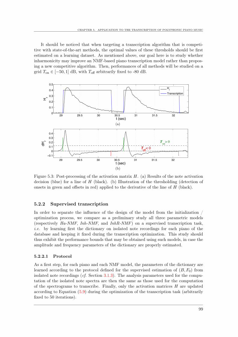
CHAPTER 5. APPLICATION TO THE TRANSCRIPTION OF POLYPHONIC PIANO MUSIC
It should be noticed that when targeting a transcription algorithm that is competi-tive with state-of-the-art methods, the optimal values of these thresholds should be firstestimated on a learning dataset. As mentioned above, our goal here is to study whetherinharmonicity may improve an NMF-based piano transcription model rather than propos-ing a new competitive algorithm. Then, performances of all methods will be studied on agrid Ton ∈ [−50, 1] dB, with Toff arbitrarily fixed to -80 dB.
29 29.5 30 30.5 31 31.5 320
0.1
0.2
0.3
0.4
0.5
t (sec)
Hr
Hr
Transcription
(a)t (sec)
29 29.5 30 30.5 31 31.5 32
0.1
0
0.1
0.2
0.3
0.4
Ton
> 0
Toff
< 0
t (sec)
dH
r
(b)
Figure 5.3: Post-processing of the activation matrix H. (a) Results of the note activationdecision (blue) for a line of H (black). (b) Illustration of the thresholding (detection ofonsets in green and offsets in red) applied to the derivative of the line of H (black).
5.2.2 Supervised transcription
In order to separate the influence of the design of the model from the initialization /optimization process, we compare as a preliminary study all three parametric models(respectively Ha-NMF, Inh-NMF, and InhR-NMF ) on a supervised transcription task,i.e. by learning first the dictionary on isolated note recordings for each piano of thedatabase and keeping it fixed during the transcription optimization. This study shouldthus exhibit the performance bounds that may be obtained using such models, in case theamplitude and frequency parameters of the dictionary are properly estimated.
5.2.2.1 Protocol
As a first step, for each piano and each NMF model, the parameters of the dictionary arelearned according to the protocol defined for the supervised estimation of (B,F0) fromisolated note recordings (cf. Section 3.1.3). The analysis parameters used for the compu-tation of the isolated note spectra are then the same as those used for the computationof the spectrograms to transcribe. Finally, only the activation matrices H are updatedaccording to Equation (5.9) during the optimization of the transcription task (arbitrarilyfixed to 50 iterations).
99

We also add a fourth supervised NMF model, denoted by Oracle-NMF, for which thedictionary is composed of the isolated note short-time spectra (H is thus optimized usingEquation (2.17)). Since all the parametric dictionaries are limited to the modeling ofa restricted set of partials (e.g. no consideration of the partials related to longitudinalvibrations of the strings or partials resulting from couplings, but also of other effectssuch as the hammer stroke noise) this latter supervised model should give a performancebound in case the tones are modeled along the whole frequency axis. Such spectra of thedictionary are illustrated on Figure 5.4 for all four methods.
0 2000 4000 6000 8000 10000
−120
−100
−80
−60
−40
−20
0
Frequency (Hz)
Mag. S
pectr
um
(dB
)
Oracle
Ha
(a)
0 2000 4000 6000 8000 10000
−120
−100
−80
−60
−40
−20
0
Frequency (Hz)
Mag. S
pectr
um
(dB
)
Oracle
Inh
(b)
0 2000 4000 6000 8000 10000
−120
−100
−80
−60
−40
−20
0
Frequency (Hz)
Mag. S
pectr
um
(dB
)
Oracle
InhR
(c)
Figure 5.4: Spectrum of the note A3 (MAPS ENSTDkAM piano) for the dictionary of (a)Ha-NMF, (b) Inh-NMF, and (c) InhR-NMF. The original spectrum (in gray) is used forthe dictionary of Oracle-NMF.
5.2.2.2 Results
The four methods are then applied to the supervised transcription of the 45 excerpts ofpieces presented in Section 5.2.1.1. For the 3 parametric models (Ha/Inh/InhR-NMF ) theinfluence of Nr, the maximal number of partials for each note, is studied on a grid havingvalues in 5, 10, 20, 30, 40, 50.
Precision, Recall and F-measure curves (averaged over the 45 pieces) as a function ofthe onset detection threshold Ton are depicted in Figure 5.5, for Nr = 20. When comparingthe four methods, one can see that refining the model of piano tone spectra leads to a
100

CHAPTER 5. APPLICATION TO THE TRANSCRIPTION OF POLYPHONIC PIANO MUSIC
higher Precision but does not improve the Recall (consistent for all methods). Thus, itseems that including more information in the dictionary model mainly helps in avoidingthe detection of FP notes. This finally results in an increase of the F-measure.
−50 −45 −40 −35 −30 −25 −20 −15 −10 −5 00
20
40
60
80
100
Ton
(dB)
Pre
cis
ion
(%
)
Ha
Inh
InhR
Oracle
(a)
−50 −45 −40 −35 −30 −25 −20 −15 −10 −5 00
20
40
60
80
100
Ton
(dB)
Re
ca
ll (%
)
Ha
Inh
InhR
Oracle
(b)
−50 −45 −40 −35 −30 −25 −20 −15 −10 −5 00
10
20
30
40
50
60
70
80
Ton
(dB)
F−
me
asu
re (
%)
Ha
Inh
InhR
Oracle
(c)
Figure 5.5: Supervised transcription performances. (a) Precision, (b) Recall, and (c) F-measure (in %) as a function of the onset detection threshold Ton (in dB) for Ha/Inh/InhR-NMF with Nr = 20, and Oracle-NMF.
The influence of Nr for the three parametric models is also presented on Figure 5.6for a detection threshold fixed to Ton = −22 dB (that corresponds approximately to thevalue leading to optimal F-measure performances for all methods). Again, increasing thenumber of partials of the spectra tends to improve the Precision but does not seem to havea significant influence on the Recall. Logically, when increasing the number of partials,the performance gap between the two inharmonic models and the harmonic model isincreasing. However, for all parametric models a limit is reached for Nr = 20. This resultis surprising (particularly for the inharmonic models for which the partials of transversevibration were accurately learned up to rank 50 in the first step) since notes below A♯4(70) are usually composed of more partials, up to more than a hundred in the bass range.A possible explanation for this may be that these experiments have been performed using
101

a KL divergence (β = 1) for the reconstruction cost-function. As highlighted in Section2.1.1.3, the KL divergence is not scale invariant and thus favors the reconstruction of thecomponents having highest magnitudes in the spectrogram. As it can be seen on Figure5.4, partials with a rank greater than 20 have magnitudes below -50 dB when comparedto the first partial. These may thus be neglected in the optimization of the activationmatrix H. It should be then interesting to study the influence of Nr on the performance,jointly with a grid of β values (for instance ∈ [0, 1])1. Indeed, such an application ofparametric NMF-based models to transcription has shown optimal performances for β =0.5 in [Vincent et al., 2010].
5 10 15 20 25 30 35 40 45 5065
70
75
80
85
Nr
Pre
cis
ion
(%
)
Ha
Inh
InhR
Oracle
(a)
5 10 15 20 25 30 35 40 45 5075
75.5
76
76.5
77
Nr
Re
ca
ll (%
)
Ha
Inh
InhR
Oracle
(b)
5 10 15 20 25 30 35 40 45 5068
70
72
74
76
78
80
Nr
F−
me
asu
re (
%)
Ha
Inh
InhR
Oracle
(c)
Figure 5.6: (a) Precision, (b) Recall and (c) F-measure (in %) obtained for all methodsas a function of the number of partials Nr for Ton = −22 dB.
Finally, the FP errors made by all methods are analyzed in detail. Each FP is classified
1Further experiments have been conducted after the writing of this thesis. When setting Nr = 50 andcomputing the supervised transcription for a grid of β having values linearly distributed in [0, 2] (step of0.1), we found that β = 0.9 leads to the highest F-measure for Inh/InhR/Oracle-NMF and β = 1 forHa-NMF.
102

CHAPTER 5. APPLICATION TO THE TRANSCRIPTION OF POLYPHONIC PIANO MUSIC
according to its distance (in semitones, modulo 12) with respect to the notes that areactually present in the ground truth within +/− 50 ms. Another class (denoted by ‘NO’)is considered for FP detected while no onset is present in the ground truth. Histogramsof these errors are presented on Figure 5.7 for all methods with Nr ∈ 5, 10, 20 andTon = −22 dB.
In accordance with the results presented above, the improvement of Precision (fromHa-NMF to Oracle-NMF, with Nr increasing) is related to a decrease of the number ofFP. The inharmonicity inclusion is relevant for Nr > 5 and interestingly, as expected,tends to mainly reduce harmonically-related FP (e.g. major thirds, fifths and octavescorresponding respectively to 4, 7 and 12 semitones).
NO 1 2 3 4 5 6 7 8 9 10 11 120
500
1000
1500
2000
Error type (in semitones, modulo 12)
FP
dis
trib
utio
n
Ha
Inh
InhR
Oracle
(a) Nr = 5
NO 1 2 3 4 5 6 7 8 9 10 11 120
200
400
600
800
1000
1200
1400
Error type (in semitones, modulo 12)
FP
dis
trib
utio
n
Ha
Inh
InhR
Oracle
(b) Nr = 10
NO 1 2 3 4 5 6 7 8 9 10 11 120
200
400
600
800
1000
1200
Error type (in semitones, modulo 12)
FP
dis
trib
utio
n
Ha
Inh
InhR
Oracle
(c) Nr = 20
Figure 5.7: Histogram of FP errors returned by all methods for different values of Nr andTon = −22 dB. Error types are given in semitones (modulo 12), except for ‘NO’ whichcorresponds to FP errors of the algorithms while no onset was present in the reference.
103

5.2.2.3 Conclusion
This preliminary study shows that increasing the precision of the piano tone spectra modelmay really improve the performance of an NMF-based transcription system, in the casewhen the parameters of the dictionary are properly estimated. In particular it helps inreducing FP detections. However, there is no guarantee that similar results are obtained inthe case of an unsupervised transcription. As mentioned in Section 2.1.2, and highlightedin Section 3.1.2.2 for piano tone analysis, the NMF cost-functions are often non-convexand special care has to be taken for the initialization and the optimization scheme, in sucha way that the algorithm converges toward the desired optimum.
5.2.3 Unsupervised transcription
Finally all three parametric models (Ha/Inh/InhR-NMF ) are evaluated on the samedataset in an unsupervised transcription task. Thus, at each loop of the optimizationalgorithms H and W θ matrices are iteratively updated.
5.2.3.1 Protocol
Initialization: For both inharmonic models, the influence of the initialization of (B,F0)parameters is investigated. Two configurations are then proposed. First, a naive initializa-tion for which F0r is set to Equal Temperament (no “octave stretching”) and Br to 5.10−3,∀r ∈ [1, R] is used. Second, (Br, F0r) parameters are initialized according to the meanmodel of inharmonicity and tuning along the whole compass of pianos presented in Section4.4.3. These two initialization configurations are respectively denoted by ‘ini1’ and ‘ini2’in the following. For Ha-NMF, F0r is simply initialized to exact Equal Temperament.
Optimization scheme: The optimization is detailed in Algorithms 4, 5 and 6, respec-tively for Ha-NMF, Inh-NMF and InhR-NMF.
It is worth noting here that the optimization for the transcription task slightly differsfrom the one presented in Section 3.1.2.3 for the supervised estimation of (B,F0). Besidesthe inclusion of the update of H and the normalization of anr values, a few modifications ofthe steps of the algorithms are done. First, we did not retain the noise level as discussed inSection 3.1.2.2, where it is used to remove the influence of partials drowned in noise; such acomponent cannot be simply adapted to a transcription application. Second, the numberof partials for each note Nr is here fixed at the initialization instead of being initializedwith a small number and iteratively increased (as done in lines 14-16 of Algorithms 1and 2, page 47). However, further work will investigate the influence of such an iterativeoptimization scheme on transcription performance as it has been shown in Section 3.1.2.2that it should help in avoiding the convergence of (B,F0) parameters toward local optima.
Learning of the regularization parameter of InhR-NMF : In order to estimate anappropriate value for the regularization parameter λ of the InhR-NMF method, a learningset composed of 9 pieces is built (1 piece for each piano, none of them in the test set). Theinfluence of λ is then studied for Nr = 10 on a grid covering the range [10−11, 10−3] withvalues logarithmically distributed. Also, as mentioned in Section 3.1.2.2, the spectrogramsare normalized to a maximal value of 1 in order to limit the influence of the scaling propertyof KL divergence in the tuning of λ. The optimal F-measure is obtained for λ = 2 · 10−5,
104

CHAPTER 5. APPLICATION TO THE TRANSCRIPTION OF POLYPHONIC PIANO MUSIC
and it should be noted that the performance did not depend on a fine tuning of thisparameter2.
Algorithm 4 Ha-NMF unsupervised transcription
1: Input:
2: V spectrogram (normalized to a max. of 1)3: β
4: Initialization: ∀ r ∈ [1, R], n ∈ [1, Nr],5: F0r according to ET6: fnr = nF0r, anr = 1,7: W θ computation (cf. Eq. (3.1))8: H with random positive values
9: Optimization:
10: for it = 1 to It do
11: • Hrt update ∀ r ∈ [1, R], t ∈ [1, T ] (Eq. (5.9))12: • anr update ∀ r ∈ [1, R], n ∈ [1, Nr] (Eq. (3.8))13: anr normalization ∀ r ∈ [1, R] (Eq. (5.12)-(5.14))14: W θ update (Eq. (3.1))15: for u = 1 to 10 do
16: • F0r update ∀r ∈ [1, R] (cf. Eq. (5.6))17: W θ update (cf. Eq. (3.1))18: end for
19: end for
20: Output: H,Br, F0r, anr
Algorithm 5 Inh-NMF unsupervised transcription
1: Input:
2: V spectrogram (normalized to a max. of 1)3: β
4: Initialization: ∀ r ∈ [1, R], n ∈ [1, Nr],5: (Br, F0r) according to ini1 or ini26: fnr = nF0r
√1 +Brn2, anr = 1,
7: W θ computation (cf. Eq. (3.1))8: H with random positive values
9: Optimization:
10: for it = 1 to It do
11: • Hrt update ∀ r ∈ [1, R], t ∈ [1, T ] (Eq. (5.9))12: • anr update ∀ r ∈ [1, R], n ∈ [1, Nr] (Eq. (3.8))13: anr normalization ∀ r ∈ [1, R] (Eq. (5.12)-(5.14))14: W θ update (Eq. (3.1))15: for u = 1 to 10 do
16: • F0r update ∀r ∈ [1, R] (cf. Eq. (3.13))17: W θ update (cf. Eq. (3.1))18: • Br update ∀r ∈ [1, R] (cf. Eq. (3.12))19: W θ update (cf. Eq. (3.1))20: end for
21: end for
22: Output: H,Br, F0r, anr
2The actual value found in [Rigaud et al., 2013c] is λ = 1. However, in this latter study the penaltyterms of InhR-NMF cost-function does not account for the constant multiplicative factor KτT introducedin this thesis (cf. Equation (3.7)). Thus, the value λ = 2 · 10−5 given in this section is considering thisscaling factor, with – according to the analysis parameters – Kτ = 17 bins and T = 2660 time-frames.
105

Algorithm 6 InhR-NMF unsupervised transcription
1: Input:
2: V spectrogram (normalized to a max. of 1)3: β, λ
4: Initialization: ∀ r ∈ [1, R], n ∈ [1, Nr],5: (Br, F0r) according to ini1 or ini26: fnr = nF0r
√1 +Brn2, anr = 1,
7: W θ computation (cf. Eq. (3.1))8: H with random positive values
9: Optimization:
10: for it = 1 to It do
11: • Hrt update ∀ r ∈ [1, R], t ∈ [1, T ] (Eq. (5.9))12: • anr update ∀ r ∈ [1, R], n ∈ [1, Nr] (Eq. (3.8))13: anr normalization ∀ r ∈ [1, R] (Eq. (5.12)-(5.14))14: W θ update (Eq. (3.1))15: • fnr update ∀ r ∈ [1, R], n ∈ [1, Nr] (Eq. (3.18))16: W θ update (Eq. (3.1))17: for v = 1 to 30 do
18: F0r update ∀r ∈ [1, R] (cf. Eq. (3.20))19: Br update ∀r ∈ [1, R] (20 times) (cf. Eq. (3.19))20: end for
21: end for
22: Output: H,Br, F0r, anr, fnr
5.2.3.2 Results
The influence of Nr, the maximal number of partials is here studied on the grid 5, 10, 20, 30for Ton ∈ [−50, 1] dB.
The Precision, Recall and F-measure performances are presented on Figure 5.8 forNr = 20. For the first initialization, Inh-NMF and InhR-NMF do not perform as well asHa-NMF (this is consistent with the observation in [Vincent et al., 2008]). Conversely, forthe second initialization with the mean model of inharmonicity and piano tuning, thesemethods perform significantly better than Ha-NMF (ANOVA p-values lower than 0.05for Nr < 30 and Ton = −18 dB). Furthermore, both inharmonic models give comparablemean F-measures (p-values higher than 0.5). Standard deviations are not reported in theplots but are around 10 to 14 %.
The influence of Nr on the performances, for Ton = −18 dB, is presented on Figure 5.9.Again, for all different values of Nr, both inharmonic models return highest performancesthan Ha-NMF in the case where the initialization of (B,F0) parameters was performedaccording the mean model of inharmonicity and tuning. In accordance with the resultsobtained for the supervised case, increasing the number of partials tends to improve theperformances of Inh/InhR-NMF up to Nr = 20. Surprisingly, the performance of Ha-NMF keeps increasing for Nr = 30. It seems here that adding more partials avoids asituation where high notes explain high rank partials belonging to lower notes. It is alsointeresting to notice that Ha-NMF results for Nr = 30 are comparable to those obtainedby the NMF under the harmonicity constraint presented in [Vincent et al., 2010] (SectionV.B) for similar experimental setups.
These experiments tend to demonstrate that such parametric NMF models with inhar-monicity constraints are highly dependent on the initialization. Indeed, the reconstructioncost function is non-convex with respect to fnr, F0r or Br parameters, and present a largenumber of local minima. Hence, multiplicative update rules (as well as other optimization
106

CHAPTER 5. APPLICATION TO THE TRANSCRIPTION OF POLYPHONIC PIANO MUSIC
−50 −45 −40 −35 −30 −25 −20 −15 −10 −5 00
10
20
30
40
50
60
70
80
90
Ton
(dB)
Pre
cis
ion
(%
)
Ha
Inh ’ini1’
InhR ’ini1’
Inh ’ini2’
InhR ’ini2’
(a)
−50 −45 −40 −35 −30 −25 −20 −15 −10 −5 00
10
20
30
40
50
60
70
80
90
Ton
(dB)
Re
ca
ll (%
)
Ha
Inh ’ini1’
InhR ’ini1’
Inh ’ini2’
InhR ’ini2’
(b)
−50 −45 −40 −35 −30 −25 −20 −15 −10 −5 00
10
20
30
40
50
60
Ton
(dB)
F−
me
asu
re (
%)
Ha
Inh ’ini1’
InhR ’ini1’
Inh ’ini2’
InhR ’ini2’
(c)
Figure 5.8: (a) Precision, (b) Recall and (c) F-measure (in %) as a function of the detectiononset threshold Ton. Performances of Ha, Inh and InhR are respectively depicted as black,blue and red curves. For Inh and InhR, dashed and plain lines respectively correspond tothe results obtained for ‘ini1’ and ‘ini2’.
methods based on gradient descent) cannot ensure that these parameters will be correctlyestimated. This results in the fact that the initialization of such parameters requires spe-cial care. Also, an alternative optimization scheme that would consider initializing thenotes with a few partials and increasing the number iteratively (as proposed in Section3.1.2.2) may be an efficient mean for avoiding the convergence toward local optima.
In contrast with the results for the supervised estimation of (B,F0) presented in Chap-ter 3, taking into account the dispersion of the partial frequencies from a theoretical in-harmonic relation in InhR-NMF does not seem valuable for a transcription task, when
107

compared to Inh-NMF. A possible explanation for this result may be that InhR-NMF wasfound particularly useful for the analysis of low-bass tones, as the deviations related to thestring-bridge couplings are mainly present in the very low pitch range. However, as shownin Figure 5.2, these notes are rarely played in a musical context. Also, introducing a largernumber of free parameters in the model may not be valuable when targeting complex taskssuch as transcription.
5 10 15 20 25 3030
35
40
45
50
55
60
65
70
Nr
Pre
cis
ion
(%
)
Ha
Inh ’ini1’
InhR ’ini1’
Inh ’ini2’
InhR ’ini2’
(a)
5 10 15 20 25 3030
35
40
45
50
55
60
65
Nr
Re
ca
ll (%
)
Ha
Inh ’ini1’
InhR ’ini1’
Inh ’ini2’
InhR ’ini2’
(b)
5 10 15 20 25 3030
35
40
45
50
55
60
65
Nr
F−
me
asu
re (
%)
Ha
Inh ’ini1’
InhR ’ini1’
Inh ’ini2’
InhR ’ini2’
(c)
Figure 5.9: (a) Precision, (b) Recall and (c) F-measure (in %) as a function of the numberof partials Nr for Ton = −18 dB. Performances of Ha, Inh and InhR are respectively de-picted as black, blue and red curves. For Inh and InhR, dashed and plain lines respectivelycorrespond to the results obtained for ‘ini1’ and ‘ini2’.
108

CHAPTER 5. APPLICATION TO THE TRANSCRIPTION OF POLYPHONIC PIANO MUSIC
5.3 Conclusion
Including inharmonicity in parametric NMF models has been shown to be relevant ina piano transcription task, provided that the inharmonicity and tuning parameters aresufficiently well estimated, this being highly dependent on the initialization. More pre-cisely, an initialization with the same average value for the inharmonicity of all notes, andEqual Temperament for the tuning, turns out to provide worse estimates than the simplerpurely harmonic model. However, a note-dependent inharmonicity law, and the corre-sponding “stretched” tuning curves, provide a good initialization to our models, that leadto significant improvement in the transcription results. Further work will investigate if anoptimization based on an iterative addition of partials in the model may still increase theperformance. Also, in order to build a competitive transcription system, additional studieswill examine how these models on partials frequencies can be combined with amplitudemodels (smooth spectral envelopes), or frame dependencies in time.
109

110
Chapter 6
Conclusions and prospects
6.1 Conclusion
In this thesis, we have tackled the issue of the modeling and the representation of musicalsounds by an approach inspired by both acoustics and signal processing perspectives. Wefocused our studies on the analysis of piano music, with particular attention paid to theinclusion of the inharmonic structure of the tones (as given by the model of transversevibration of stiff strings) in signal-based modelings. To this end, two frameworks havebeen presented in Section 3.
We first considered enforcing the inharmonicity in the dictionary of spectra of NMF-based models. Two different ways of including such a constraint have been studied. Thefirst one strictly enforces the partial frequencies of the model to follow the inharmonic-ity relation (Inh-NMF model). The second one includes inharmonicity by considering aregularized problem, i.e. by adding a penalization term to the NMF reconstruction cost-function (InhR-NMF model). Optimization algorithms as well as practical considerationshave been given for both models in order to perform the estimation of the parameters.
We then introduced a probabilistic line spectrum model (PLS ). From a prior peak-picking in time-frequency representations, the model assumes that the observed frequen-cies have been generated by a mixture of notes, each being composed of partial and noisecomponents. The partial components are modeled by Gaussian mixtures having meansconstrained by the inharmonicity relation parameters. The proposed optimization algo-rithm returns a classification of each observation in partial and noise components for eachnote as well as their inharmonicity relation parameters and the probability for each noteto have generated the observations of each time-frame.
Such models have been successfully applied to both acoustics and signal processingapplications giving answers to the issues raised in the introduction:
• Can such classes of models be used to efficiently learn physics-related parameters (e.g.information about the design and tuning) of a specific instrument?
In Chapter 3 we focused on the precise estimation of the inharmonicity coefficientB and the F0 of piano tones. All models have been tested on the whole compass of 11different pianos in order to access the robustness with respect to the variability of thetones. These have been compared favorably to one state the art algorithm.
111

Both NMF-based models have been successfully applied to the supervised (i.e. havingthe knowledge of the played notes) estimation of (B,F0) of isolated note and chord record-ings. In this context, the relaxed inclusion of the inharmonicity constraint in InhR-NMFhas shown benefits in allowing for slight deviations of the partial frequencies around theinharmonicity relation (as for instance caused by the string-bridge coupling).
On the same dataset of isolated note recordings, the PLS model has shown benefitsin still performing well for a large range of the piano compass in the context of an un-supervised analysis. It has also been applied on a generic polyphonic piece of music, forwhich (B,F0) parameters were accurately learned for a restricted set of notes that wereplayed. Interestingly for the proposed application a perfect transcription of the music didnot seem necessary.
In Chapter 4, a model for the inharmonicity and the tuning variations along the wholepiano compass have been presented. While considering a small set of high-level parame-ters (only 6 global parameters to account for the main trends of 88× 2 string parameters)these models have been found useful for various applications. In particular these havebeen applied to the retrieval of parameters highlighting some tuner’s choices on differentpiano types, the generation of tuning curves for out-of-tune pianos or piano synthesizers,the initialization of the inharmonicity coefficient and the F0 of analysis algorithms, andfinally to the interpolation of inharmonicity and tuning along the whole compass of apiano from a prior estimation of these parameters on a restricted set of notes played in apolyphonic piece of music.
• Does refining/complexifying generic signal models actually improve the performance ofanalysis tasks targeted by the MIR community?
In Chapter 5, the two inharmonic NMF-based models have been applied to a tran-scription task and compared to a simpler harmonic model. The results have shown thatinharmonicity inclusion was relevant in transcription tasks, in particular because it helpsin reducing the detection of False Positives corresponding to harmonically-related notes(thirds, fifths and octaves). However, the performances of such models are highly depen-dent on the initialization of (B,F0) parameters because of the non-convexity, with respectto these parameters, of the cost-functions. Thus, it has been found, in accordance withprevious studies, that a naive initialization of such parameters can lead to a degradationof the results, when compared to a simpler harmonic model. Conversely, the use of amean model of inharmonicity and tuning along the whole compass (introduced in Chap-ter 4) for the initialization has shown here a significant improvement in the transcriptionperformances. The investigation of alternative optimization schemes that should be lesssensitive to local optima will be investigated in further studies.
6.2 Prospects
6.2.1 Building a competitive transcription system
All the models that have been presented in this thesis focus on the inclusion of the inhar-monic structure of the piano tones. However, when targeting the design of a competitivetranscription system, a few more elements of sound modeling have to be taken into ac-
112

CHAPTER 6. CONCLUSIONS AND PROSPECTS
count. This could consist in constraining the shape of the spectral envelopes of the spectra(possibly varying over time in order to account for the fact that high rank partials are de-caying faster than low ranks in piano tones) or the temporal activations. Such modelingshave been widely investigated in the literature on NMF (as detailed in Section 2.1.2) andshould be easily adapted to our model formulation. Including such additional informa-tion in the unsupervised transcription algorithm should also help obtaining more robustestimates of (B,F0) parameters. While performing the transcription of a piece of music,one could imagine retrieving the model of piano that has been played by comparing theB estimates with reference curves of inharmonicity of several pianos.
Future research may also be conducted on the extension of the model to poly-instrumentalmusic composed of harmonic and inharmonic instruments (possibly combining Ha-NMFand Inh-NMF models). This could be of interest in order to investigate whether inhar-monicity is able to lift ambiguities of harmonically-related notes played by different in-struments (e.g. C on piano and G on trumpet) while providing a clustering of all detectednotes in the different instruments of the model.
6.2.2 Extension to other string instruments
The models that have been presented in this thesis are sufficiently generic to be appliedto other struck but also plucked string instruments, such as for instance the harpsichord,the guitar or the harp. However, as it has been shown for the case of the piano, a priorstudy of the variations of (B,F0) parameters along the compass seems essential for theinitialization of the algorithms.
We propose here some prospects for an application to the guitar. As for the piano,some invariants in the design of the instruments can be used to build parametric modelsfor the inharmonicity along the whole compass. Figure 6.1 presents the evolution of theinharmonicity coefficient along the register covered by the 6 strings of an electric guitar(e, B, G and D, A, E respectively correspond to plain and wrapped set of strings). Thesehave been estimated on isolated note recordings using InhR-NMF model according tothe protocol detailed in Section 3.1.3.2, with a manual tuning for the initialization of theparameters. One can notice here that the evolution of the inharmonicity coefficient alongthe range covered by each string has a linear behavior in logarithmic scale. For eachstring, the slope is related to the position of the frets that modify the vibrating lengthof the string. For most guitars the fret position is designed so that the guitar is tunedaccording to Equal Temperament. Thus, in the case where the tension is constant (nostring bending), according to the expression of B (Equation (2.24)), the slope is equalto log 22m/12, where m denotes the MIDI note index (as depicted in gray dashed lines inFigure 6.1). Then, in order to model the inharmonicity variations along the compass of aguitar, one could consider 6 different parameters corresponding to the Y-intercept of thestraight lines (the jump between the 6 lines being mainly affected by the changes in thestring diameters).
As the guitar allows us to play the same note with different combinations of string/ neck position, such a parametric model of inharmonicity may potentially be used inaudio to tablature transcription tasks [Barbancho et al., 2012], where beyond retrievingthe notes that are played, inharmonicity could help here in assessing the position of theplayer’s fingers along the guitar neck (as illustrated on Figure 6.2).
113

40 45 50 55 60 65 70 75 80 85
105
104
103
2(2.m/12)
m (note in MIDI index)
B (
log
. sca
le)
E
A
D
G
B
e
Figure 6.1: Inharmonicity curves along the range covered by the 6 strings of an electricguitar.
(a)
40 45 50 55 60 65 70 75 80 85
10−4
10−3
m (note in MIDI index)
B (
log. scale
)
Am pos. 1
Am pos. 2
(b)
Figure 6.2: (a) A Minor (Am) chord played for two different positions on the guitar neck.(b) Inharmonicity patterns for the two positions.
114
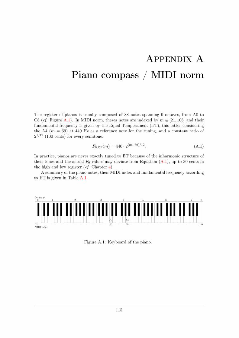
Appendix A
Piano compass / MIDI norm
The register of pianos is usually composed of 88 notes spanning 9 octaves, from A0 toC8 (cf. Figure A.1). In MIDI norm, theses notes are indexed by m ∈ [21, 108] and theirfundamental frequency is given by the Equal Temperament (ET), this latter consideringthe A4 (m = 69) at 440 Hz as a reference note for the tuning, and a constant ratio of21/12 (100 cents) for every semitone:
F0,ET(m) = 440 · 2(m−69)/12. (A.1)
In practice, pianos are never exactly tuned to ET because of the inharmonic structure oftheir tones and the actual F0 values may deviate from Equation (A.1), up to 30 cents inthe high and low register (cf. Chapter 4).
A summary of the piano notes, their MIDI index and fundamental frequency accordingto ET is given in Table A.1.
Figure A.1: Keyboard of the piano.
115

Octave C C ♯ D E E F F ♯ G G ♯ A B B# (Do) (Do ♯) (Ré) (Mi ) (Mi) (Fa) (Fa ♯) (Sol) (Sol ♯) (La) (Si ) (Si)
0 (-1)21 22 23 MIDI index
27.50 29.13 30.86 F0ET (Hz)
1 (0)24 25 26 27 28 29 30 31 32 33 34 35 MIDI index
32.70 34.64 36.70 38.89 41.20 43.65 46.24 48.99 51.91 55.00 58.27 61.73 F0ET (Hz)
2 (1)36 37 38 39 40 41 42 43 44 45 46 47 MIDI index
65.40 69.29 73.41 77.78 82.40 87.30 92.49 97.99 103.82 110.00 116.54 123.47 F0ET (Hz)
3 (2)48 49 50 51 52 53 54 55 56 57 58 59 MIDI index
130.81 138.59 146.83 155.56 164.81 174.61 184.99 195.99 207.65 220.00 233.08 246.94 F0ET (Hz)
4 (3)60 61 62 63 64 65 66 67 68 69 70 71 MIDI index
261.62 277.18 293.66 311.12 329.62 349.22 369.99 391.99 415.30 440 466.16 493.88 F0ET (Hz)
5 (4)72 73 74 75 76 77 78 79 80 81 82 83 MIDI index
523.25 554.36 587.32 622.25 659.25 698.45 739.98 783.99 830.60 880 932.32 987.76 F0ET (Hz)
6 (5)84 85 86 87 88 89 90 91 92 93 94 95 MIDI index
1046.50 1108.73 1174.65 1244.50 1318.51 1396.91 1479.97 1567.98 1661.21 1760.00 1864.65 1975.53 F0ET (Hz)
7 (6)96 97 98 99 100 101 102 103 104 105 106 107 MIDI index
2093.00 2217.46 2349.31 2489.01 2637.02 2793.82 2959.95 3135.96 3322.43 3520.00 3729.31 3951.06 F0ET (Hz)
8 (7)108 MIDI index
4186.01 F0ET (Hz)
Table A.1: Correspondence between notes, MIDI indices and fundamental frequencies given by ET along the compass of the piano.French notations for the notes and octave numbers are given in parenthesis.
116

Appendix B
Noise level estimation
This appendix presents the noise level estimation method used in the pre-processing stepof the (B,F0) estimation algorithms introduced in Chapter 3. The method assumes anadditive colored noise, i.e. generated by the filtering of a white Gaussian noise and addedto the signal of interest [Yeh and Röbel, 2006]. In a given narrow band, if the noise filtershave a quasi flat frequency response, the noise can be considered as white Gaussian andits spectral magnitude follows a Rayleigh distribution:
p(xf ;σf ) =xfσ2f
· e−x2f/(2σ2
f) , xf ∈ [0,+∞[. (B.1)
In this pre-processing stage, we want to estimate the noise distribution in each bandwithout removing the partials. To do so, a good estimator for σf is the median medf =σf√log 4. Indeed, when the length of the analysis window is adapted to the resolution,
in a given narrow band, there are much less bins corresponding to partials than binscorresponding to noise, so partials have a reduced influence on the estimate of the noisemedian. The tradeoff sits in the choice of the bandwidth: the bands have to be narrowenough so that the white noise approximation holds, but wide enough so that most of thebins correspond to noise. We chose a 300Hz median filtering on the magnitude spectrumS(f) to estimate σf . Finally, we define the noise level in each band NL(f) as the magnitudesuch that the cumulative distribution function is equal to a given threshold T , set toT = 0.9999. With this choice of T , only 6 bins corresponding to noise on average (outof 216) should be above the noise level. The cumulative density function of a Rayleighdistribution is given by:
c(xf ;σf ) = 1− e−x2f/(2σ2
f). (B.2)
Thus the noise level can be expressed as:
NL(f) =medf√log 4
·√2 log
1
1− T. (B.3)
An illustration of the noise level computation for a note C4 is given in Figure B.1.
117

0 1000 2000 3000 4000 5000 6000 7000 8000 9000 10000 11000
−80
−60
−40
−20
0
20
40
Frequency (Hz)
Ma
g.
sp
ectr
um
(d
B)
spectrum
median filtering
Noise Level
Figure B.1: Noise level computation for the magnitude spectrum of a note C4.
118

Appendix C
Derivation of Inh/InhR/Ha-NMF
update rules
This appendix presents the mathematical derivation of the update rules used in the op-timization of Inh/InhR-NMF (cf. Section 3.1.2.1) and Ha-NMF (cf. Section 5.2.1.2)models.
C.1 Multiplicative update rules
As presented in Section 2.1.1.5, multiplicative update rules can be obtained by decompos-ing the partial derivative of a cost-function, with respect to a given parameter θ∗, as adifference of two positive terms:
∂C(θ∗)∂θ∗
= P (θ∗)−Q(θ∗), P (θ∗), Q(θ∗) ≥ 0. (C.1)
In the case the cost-function includes a regularization term, for instance in the form
C(θ) = C0(θ) + λ · C1(θ, γ), (C.2)
the same kind of decomposition can be performed independently for each term so that
∂C(θ∗, γ)∂θ∗
= (P0(θ∗) + λ · P1(θ
∗))︸ ︷︷ ︸P (θ∗)
− (Q0(θ∗) + λ ·Q1(θ
∗))︸ ︷︷ ︸Q(θ∗)
, (C.3)
Then, the parameter is updated as follows:
θ∗ ← θ∗ ×Q(θ∗)/P (θ∗) (C.4)
C.2 Partial derivatives of the reconstruction cost-function
C.2.1 Problem reminder
For all three parametric models, the reconstruction cost-function is given by (cf. Section3.1.1):
C0(θ,H) =∑
k∈K
T∑
t=1
dβ
(Vkt | Vkt
), (C.5)
119

where
Vkt =
R∑
r=1
W θrkr ·Hrt, (C.6)
and
W θrkr =
Nr∑
n=1
anr · gτ (fk − fnr), (C.7)
with θr = anr, fnr | n ∈ [1, Nr], and K = k | fk ∈ fnr + [−2/τ, 2/τ ], ∀n ∈ [1, Nr], ∀r ∈[1, R].
C.2.2 Derivative with respect to θ
According to the partial derivative of β-divergences (∂dβ(x | y)/∂y, cf. Equation (2.10)),the partial derivative of the reconstruction cost-function with relation to a specific param-eter θ∗ ∈ θ is given by:
∂C0(θ,H)
∂θ∗=∑
k∈K
T∑
t=1
∂Vkt
∂θ∗· V β−2
kt (Vkt − Vkt), (C.8)
with
∂Vkt
∂θ∗=
R∑
r=1
∂W θrkr
∂θ∗·Hrt, (C.9)
which can be decomposed as a difference of two positive terms
∂Vkt
∂θ∗=
R∑
r=1
∂W θr ⊕kr
∂θ∗·Hrt
︸ ︷︷ ︸∂V
⊕
kt∂θ∗
−R∑
r=1
∂W θr ⊖
kr
∂θ∗·Hrt
︸ ︷︷ ︸∂V
⊖
kt∂θ∗
. (C.10)
Finally, the quantity ∂C0(θ,H)/∂θ∗ can also be expressed as a difference of two positivequantities:
∂C0(θ,H)
∂θ∗=∑
k∈K
T∑
t=1
[∂V ⊕
kt
∂θ∗· V β−1
kt +∂V ⊖
kt
∂θ∗· V β−2
kt · Vkt
]
︸ ︷︷ ︸P0(θ∗)≥0
−∑
k∈K
T∑
t=1
[∂V ⊕
kt
∂θ∗· V β−2
kt · Vkt +∂V ⊖
kt
∂θ∗· V β−1
kt
]
︸ ︷︷ ︸Q0(θ∗)≥0
.
(C.11)
C.2.2.1 Derivative with respect to anr
∀r ∈ [1, R] and n ∈ [1, Nr]
∂Vkt
∂anr= gτ (fk − fnr) ·Hrt > 0 (C.12)
120

APPENDIX C. DERIVATION OF INH/INHR/HA-NMF UPDATE RULES
It is then chosen,
∂V ⊕kt∂anr
= gτ (fk − fnr) ·Hrt,
∂V ⊖
kt
∂anr= 0.
(C.13)
Finally, by replacing in Equation (C.11), Equations (3.9) and (3.10) are obtained:
P0(anr) =∑
k∈Knr
T∑
t=1
[(gτ (fk − fnr).Hrt) .V
β−1kt
],
Q0(anr) =∑
k∈Knr
T∑
t=1
[(gτ (fk − fnr).Hrt) .V
β−2kt .Vkt
],
with Knr = k | fk ∈ fnr + [−2/τ, 2/τ ].
C.2.2.2 Derivative with respect to fnr, F0r and Br
• InhR-NMF :∀r ∈ [1, R] and n ∈ [1, Nr]
∂Vkt
∂fnr= −anr · g′τ (fk − fnr) ·Hrt (C.14)
Regardless the analysis window that has been used, the quantity g′τ (fk − fnr) changes itssign on each lobe of gτ . In order to obtain a satisfying expression (i.e. a difference of twopositive terms), the spectral support of gτ (fk−fnr) is limited to its main lobe (so the signof its derivative is changing once) and its derivative is expressed as:
g′τ (fk − fnr) = (fnr − fk) ·−g′τ (fk − fnr)
fk − fnr. (C.15)
The quantity −g′τ (fk−fnr)fk−fnr
stays positive on the main lobe, for every kind of analysis window(an illustration can be found in [Hennequin et al., 2010]). Thus,
∂V ⊕kt∂fnr
= anr · fk ·−g′τ (fk − fnr)
fk − fnr·Hrt,
∂V ⊖
kt
∂fnr= anr · fnr ·
−g′τ (fk − fnr)
fk − fnr·Hrt.
(C.16)
121

And finally, by replacing in Equation (C.11), Equations (3.21) and (3.22) are obtained:
P InhR0 (fnr) =
∑
k∈Knr
T∑
t=1
[(anr−fk.g′τ (fk − fnr)
fk − fnr.Hrt
).V β−1
kt
+
(anr−fnr.g′τ (fk − fnr)
fk − fnr.Hrt
).V β−2
kt .Vkt
],
QInhR0 (fnr) =
∑
k∈Knr
T∑
t=1
[(anr−fk.g′τ (fk − fnr)
fk − fnr.Hrt
).V β−2
kt .Vkt
+
(anr−fnr.g′τ (f − fnr)
fk − fnr.Hrt
).V β−1
kt
],
Very similar decompositions can be performed for Inh-NMF and Ha-NMF. We just givehere the expression of the partial derivatives of Vkt.
• Inh-NMF : fnr = nF0r
√1 +Brn2
∀r ∈ [1, R]
∂Vkt
∂Br= −
Nr∑
n=1
Cnr · anr · g′τ (fk − fnr) ·Hrt, (C.17)
∂Vkt
∂F0r= −
Nr∑
n=1
Dnr · anr · g′τ (fk − fnr) ·Hrt, (C.18)
with
Cnr =∂fnr∂Br
=n3F0r
2√1 +Brn2
, (C.19)
Dnr =∂fnr∂F0r
= n√1 +Brn2. (C.20)
• Ha-NMF : fnr = nF0r
∀r ∈ [1, R]
∂Vkt
∂F0r= −
Nr∑
n=1
n · anr · g′τ (fk − fnr) ·Hrt, (C.21)
(C.22)
C.2.3 Derivative with respect to Hrt
Similarly to Equation (C.8), the partial derivative of C0 with respect to Hrt can beexpressed as:
∂C0(θ,H)
∂Hrt=∑
k∈Kr
T∑
t=1
W θrkr · V
β−2kt (Vkt − Vkt), (C.23)
122

APPENDIX C. DERIVATION OF INH/INHR/HA-NMF UPDATE RULES
with Kr = k | fk ∈ fnr + [−2/τ, 2/τ ], ∀n ∈ [1, Nr]. A straightforward decomposition inthe form
∂C0(θ,H)
∂Hrt=∑
k∈Kr
T∑
t=1
W θrkr · V
β−1kt
︸ ︷︷ ︸P0(Hrt)
−∑
k∈Kr
T∑
t=1
W θrkr · V
β−2kt Vkt
︸ ︷︷ ︸Q0(Hrt)
, (C.24)
leads thus to the update rule given in Equation (5.9).
C.3 Partial derivatives of the regularization term of InhR-
NMF
C1(fnr, γr) = KτT ·R∑
r=1
Nr∑
n=1
(fnr − nF0r
√1 +Brn2
)2, (C.25)
where Kτ = Cardfk ∈ [−2/τ, 2/τ ] is the number of frequency-bins for which the partialsof the model are defined and T is the number of time-frames T .
C.3.1 Derivative with respect to fnr
∀r ∈ [1, R], n ∈ [1, Nr]
∂C1
∂fnr= KτT · 2
(fnr − nF0r
√1 +Brn2
)(C.26)
Then Equations (3.23) and (3.24) are directly obtained:
P1(fnr) = KτT · 2fnr,Q1(fnr) = KτT · 2nF0r
√1 +Brn2.
C.3.2 Derivative with respect to Br
∀r ∈ [1, R]:
∂C1
∂Br= KτT ·
Nr∑
n=1
2(fnr − nF0r
√1 +Brn2
)· −n3F0r
2√1 +Brn2
= KτT · F0r
Nr∑
n=1
(n4F0r −
n3fnr√1 +Brn2
)(C.27)
Thus, Equations (3.25) and (3.26) are obtained:
P1(Br) = F0r
Nr∑
n=1
n4,
Q1(Br) =
Nr∑
n=1
n3fnr√1 +Brn2
.
123

C.3.3 Derivative with respect to F0r
∀r ∈ [1, R]:
∂C1
∂F0r= KτT ·
Nr∑
n=1
2(fnr − nF0r
√1 +Brn2
)·(−n√
1 +Brn2). (C.28)
An exact analytic solution allows to cancel the partial derivative (corresponding to theupdate rule (3.20)):
F0r =
Nr∑n=1
fnrn√1 +Brn2
Nr∑n=1
n2(1 +Brn2)
.
124

Appendix D
(B,F0) curves along the wholecompass estimated by the
NMF-based models
This appendix presents the results for the estimation of (B,F0) from isolated note record-ings along the whole compass of the 11 considered pianos. The details of the experimentalprotocol are given in Section 3.1.3.2. The initialization of (B,F0) is depicted as blackdashed lines and the blue and red curves respectively correspond to the estimates obtainedby Inh-NMF and InhR-NMF algorithms. Note that some estimates may be missing whenthe notes were not given in the databases.
• Iowa database:
20 30 40 50 60 70 80 90 100
10−4
10−3
10−2
m (note in MIDI index)
B (
log
. sca
le)
ini
Inh−NMF
InhR−NMF
(a)
20 30 40 50 60 70 80 90 100
−20
−15
−10
−5
0
5
10
15
m (note in MIDI index)
F0/F
0,E
T (
ce
nts
)
ini
Inh−NMF
InhR−NMF
(b)
Figure D.1: Iowa (a) B and (b) F0 as dev. from ET along the whole compass.
125

• RWC database:
20 30 40 50 60 70 80 90 100
10−4
10−3
10−2
m (note in MIDI index)
B (
log
. sca
le)
ini
Inh−NMF
InhR−NMF
(a)
20 30 40 50 60 70 80 90 100−15
−10
−5
0
5
10
15
20
25
30
m (note in MIDI index)
F0/F
0,E
T (
ce
nts
)
ini
Inh−NMF
InhR−NMF
(b)
Figure D.2: RWC1 (a) B and (b) F0 as dev. from ET along the whole compass.
20 30 40 50 60 70 80 90 100
10−4
10−3
10−2
m (note in MIDI index)
B (
log
. sca
le)
ini
Inh−NMF
InhR−NMF
(a)
20 30 40 50 60 70 80 90 100−15
−10
−5
0
5
10
15
20
m (note in MIDI index)
F0/F
0,E
T (
ce
nts
)
ini
Inh−NMF
InhR−NMF
(b)
Figure D.3: RWC2 (a) B and (b) F0 as dev. from ET along the whole compass.
126

APPENDIX D. (B,F0) CURVES ALONG THE WHOLE COMPASS ESTIMATED BY THE NMF-BASED MODELS
20 30 40 50 60 70 80 90 100
10−4
10−3
10−2
m (note in MIDI index)
B (
log
. sca
le)
ini
Inh−NMF
InhR−NMF
(a)
20 30 40 50 60 70 80 90 100−10
−5
0
5
10
15
20
25
30
m (note in MIDI index)
F0/F
0,E
T (
ce
nts
)
ini
Inh−NMF
InhR−NMF
(b)
Figure D.4: RWC3 (a) B and (b) F0 as dev. from ET along the whole compass.
• MAPS database:
20 30 40 50 60 70 80 90 100
10−4
10−3
10−2
m (note in MIDI index)
B (
log
. sca
le)
ini
Inh−NMF
InhR−NMF
(a)
20 30 40 50 60 70 80 90 100−25
−20
−15
−10
−5
0
5
10
15
m (note in MIDI index)
F0/F
0,E
T (
ce
nts
)
ini
Inh−NMF
InhR−NMF
(b)
Figure D.5: AkPnBcht (a) B and (b) F0 as dev. from ET along the whole compass.
127
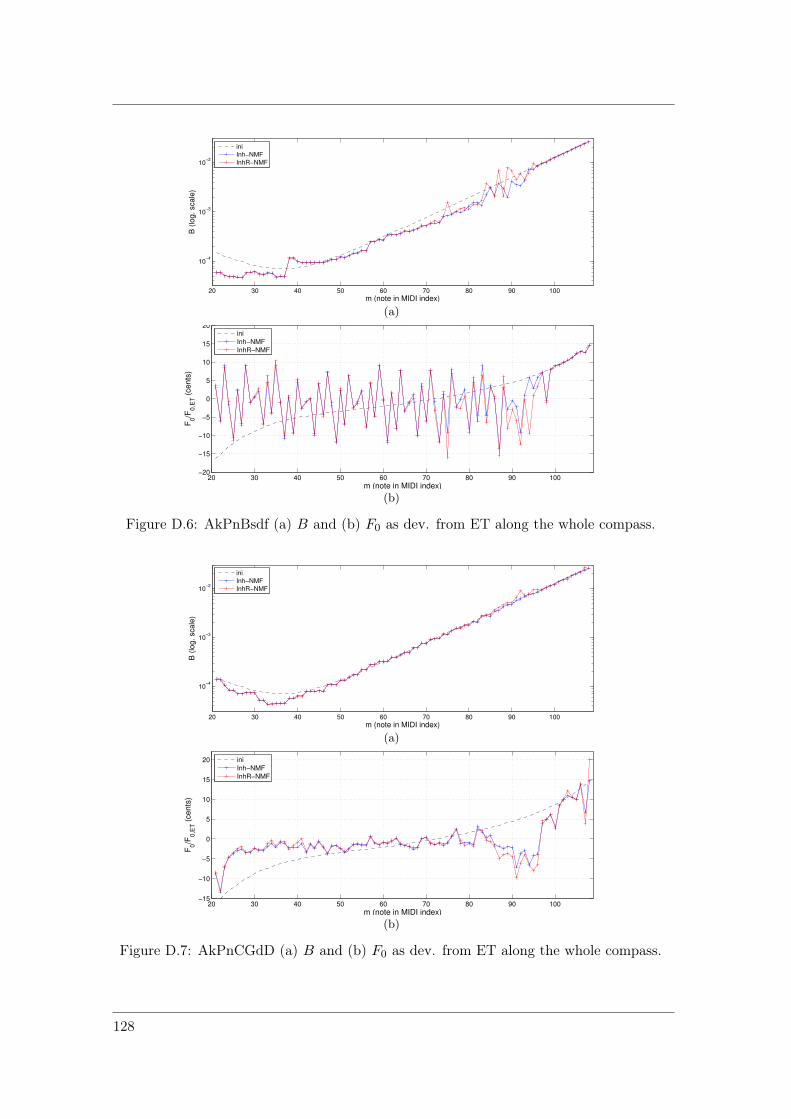
20 30 40 50 60 70 80 90 100
10−4
10−3
10−2
m (note in MIDI index)
B (
log
. sca
le)
ini
Inh−NMF
InhR−NMF
(a)
20 30 40 50 60 70 80 90 100−20
−15
−10
−5
0
5
10
15
20
m (note in MIDI index)
F0/F
0,E
T (
ce
nts
)
ini
Inh−NMF
InhR−NMF
(b)
Figure D.6: AkPnBsdf (a) B and (b) F0 as dev. from ET along the whole compass.
20 30 40 50 60 70 80 90 100
10−4
10−3
10−2
m (note in MIDI index)
B (
log
. sca
le)
ini
Inh−NMF
InhR−NMF
(a)
20 30 40 50 60 70 80 90 100−15
−10
−5
0
5
10
15
20
m (note in MIDI index)
F0/F
0,E
T (
ce
nts
)
ini
Inh−NMF
InhR−NMF
(b)
Figure D.7: AkPnCGdD (a) B and (b) F0 as dev. from ET along the whole compass.
128
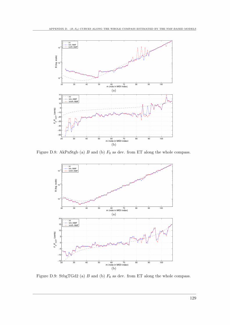
APPENDIX D. (B,F0) CURVES ALONG THE WHOLE COMPASS ESTIMATED BY THE NMF-BASED MODELS
20 30 40 50 60 70 80 90 100
10−4
10−3
10−2
m (note in MIDI index)
B (
log
. sca
le)
ini
Inh−NMF
InhR−NMF
(a)
20 30 40 50 60 70 80 90 100
−60
−50
−40
−30
−20
−10
0
10
20
30
m (note in MIDI index)
F0/F
0,E
T (
ce
nts
)
ini
Inh−NMF
InhR−NMF
(b)
Figure D.8: AkPnStgb (a) B and (b) F0 as dev. from ET along the whole compass.
20 30 40 50 60 70 80 90 100
10−4
10−3
10−2
m (note in MIDI index)
B (
log
. sca
le)
ini
Inh−NMF
InhR−NMF
(a)
20 30 40 50 60 70 80 90 100−15
−10
−5
0
5
10
15
20
m (note in MIDI index)
F0/F
0,E
T (
ce
nts
)
ini
Inh−NMF
InhR−NMF
(b)
Figure D.9: StbgTGd2 (a) B and (b) F0 as dev. from ET along the whole compass.
129

20 30 40 50 60 70 80 90 100
10−4
10−3
10−2
m (note in MIDI index)
B (
log
. sca
le)
ini
Inh−NMF
InhR−NMF
(a)
20 30 40 50 60 70 80 90 100−20
−15
−10
−5
0
5
10
15
20
25
30
35
m (note in MIDI index)
F0/F
0,E
T (
ce
nts
)
ini
Inh−NMF
InhR−NMF
(b)
Figure D.10: ENSTDkAm (a) B and (b) F0 as dev. from ET along the whole compass.
20 30 40 50 60 70 80 90 100
10−4
10−3
10−2
m (note in MIDI index)
B (
log
. sca
le)
ini
Inh−NMF
InhR−NMF
(a)
20 30 40 50 60 70 80 90 100−20
−15
−10
−5
0
5
10
15
20
25
30
35
m (note in MIDI index)
F0/F
0,E
T (
ce
nts
)
ini
Inh−NMF
InhR−NMF
(b)
Figure D.11: ENSTDkCl (a) B and (b) F0 as dev. from ET along the whole compass.
130

APPENDIX D. (B,F0) CURVES ALONG THE WHOLE COMPASS ESTIMATED BY THE NMF-BASED MODELS
20 30 40 50 60 70 80 90 100
10−4
10−3
10−2
m (note in MIDI index)
B (
log
. sca
le)
ini
Inh−NMF
InhR−NMF
(a)
20 30 40 50 60 70 80 90 100−15
−10
−5
0
5
10
15
20
m (note in MIDI index)
F0/F
0,E
T (
ce
nts
)
ini
Inh−NMF
InhR−NMF
(b)
Figure D.12: SptkBGAm (a) B and (b) F0 as dev. from ET along the whole compass.
20 30 40 50 60 70 80 90 100
10−4
10−3
10−2
m (note in MIDI index)
B (
log
. sca
le)
ini
Inh−NMF
InhR−NMF
(a)
20 30 40 50 60 70 80 90 100−15
−10
−5
0
5
10
15
20
m (note in MIDI index)
F0/F
0,E
T (
ce
nts
)
ini
Inh−NMF
InhR−NMF
(b)
Figure D.13: SptkBGCL (a) B and (b) F0 as dev. from ET along the whole compass.
131

132

Bibliography
Author’s publications
— Peer-reviewed journal article —
Rigaud, F., David, B., and Daudet, L. (2013a). A parametric model and estimationtechniques for the inharmonicity and tuning of the piano. Journal of the AcousticalSociety of America, 133(5):3107–3118.
— Peer-reviewed conference articles —
Rigaud, F., David, B., and Daudet, L. (2011). A parametric model of piano tuning.In Proceedings of the 14th International Conference on Digital Audio Effects (DAFx),pages 393–399.
Rigaud, F., David, B., and Daudet, L. (2012). Piano sound analysis using non-negativematrix factorization with inharmonicity constraint. In Proceedings of the 20th EuropeanSignal Processing Conference (EUSIPCO), pages 2462–2466.
Rigaud, F., Drémeau, A., David, B., and Daudet, L. (2013b). A probabilistic line spectrummodel for musical instrument sounds and its application to piano tuning estimation. InProceedings of the IEEE Workshop on Applications of Signal Processing to Audio andAcoustics (WASPAA).
Rigaud, F., Falaize, A., David, B., and Daudet, L. (2013c). Does inharmonicity improvean NMF-based piano transcription model? In Proceedings of the IEEE InternationalConference on Acoustics, Speech and Signal Processing (ICASSP), pages 11–15.
Manuscript references
Allen, J. B. (1977). Short term spectral analysis, synthesis, and modification by discretefourier transform. IEEE Transactions on Acoustics, Speech, and Signal Processing,25(3):235–238.
Aramaki, M., Bensa, J., Daudet, L., Guillemain, P., and Kroland-Martinet, R. (2001).Resynthesis of coupled piano string vibrations based on physical modeling. Journal ofNew Music Research (Taylor & Francis Group), 30(3):213–226.
Badeau, R., Bertin, N., and Vincent, E. (2010). Stability analysis of multiplicative updatealgorithms and application to non-negative matrix factorization. IEEE Transactions onNeural Networks, 21(12):1869–1881.
133
Badeau, R., David, B., and Richard, G. (2006). High-resolution spectral analysis of mix-tures of complex exponentials modulated by polynomials. IEEE Transactions on SignalProcessing, 54(4):1341–1350.
Bank, B. and Lehtonen, H.-M. (2010). Perception of longitudinal components in pianostring vibrations. Journal of the Acoustical Society of America (JASA express letters),128(3):117–123.
Bank, B. and Sujbert, L. (2005). Generation of longitudinal vibrations in piano strings:From physics to sound synthesis. Journal of the Acoustical Society of America,117(4):2268–2278.
Bank, B., Zambon, S., and Fontana, F. (2010). A modal-based real-time piano synthesizer.IEEE Transactions on Audio, Speech, and Language Processing, 18(4):809–821.
Barbancho, I., Tardón, L. J., Sammartino, S., and Barbancho, A. M. (2012).Inharmonicity-based method for the automatic generation of guitar tablature. IEEETransactions on Acoustics, Speech, and Signal Processing, 20(6):1857–1868.
Bello, J. P., Daudet, L., and Sandler, M. B. (2008). Automatic piano transcription usingfrequency and time-domain information. IEEE Transactions on Audio, Speech, andLanguage Processing, 14(6):2241–2251.
Benetos, E. (2012). Automatic Transcription of Polyphonic Music Exploiting TemporalEvolution. PhD thesis, School of Electronic Engineering and Computer Science QueenMary University of London.
Benetos, E. and Dixon, S. (2011). Joint multi-pitch detection using harmonic envelopeestimation for polyphonic music transcription. IEEE Journal of Selected Topics in SignalProcessing, 5(6):1111–1123.
Benetos, E. and Kotropoulos, C. (2008). A tensor-based approach for automatic musicgenre classification. In Proceedings of the 16th European Signal Processing Conference(EUSIPCO).
Benetos, E., Kotti, M., and Kotropoulos, C. (2006). Musical instrument classification usingnon-negative matrix factorization algorithms. In Proceedings of the IEEE InternationalConference on Acoustics, Speech and Signal Processing (ICASSP), pages 221–224.
Bensa, J. (2003). Analyse et synthèse de sons de piano par modèles physiques et de signaux.PhD thesis, Université de la méditerranée Aix-Marseille II.
Bensa, J., Bilbao, S., Kroland-Martinet, R., and Julius O. Smith, I. (2003). The simulationof piano string vibration: From physical models to finite difference schemes and digitalwaveguides. Journal of the Acoustical Society of America, 114(2):1095–1107.
Bertin, N. (2009). Les factorisations en matrices non-négatives. Approches contraintes etprobabilistes, application à la transcription automatique de musique polyphonique. PhDthesis, EDITE Télécom-Paristech.
134

BIBLIOGRAPHY
Bertin, N., Badeau, R., and Vincent, E. (2009). Fast bayesian NMF algorithms enforcingharmonicity and temporal continuity in polyphonic music transcription. In Proceedingsof the IEEE Workshop on Applications of Signal Processing to Audio and Acoustics(WASPAA), pages 29–32.
Bertin, N., Badeau, R., and Vincent, E. (2010). Enforcing harmonicity and smoothness inbayesian non-negative matrix factorization applied to polyphonic music transcription.IEEE Transactions on Audio, Speech and Language Processing, 18(3):538–549.
Blackham, E. (1965). The physics of the piano. Scientific American, 213:88–99.
Blanco-Martín, E., Casajus-Quiros, F. J., and Ortiz-Berenguer, L. I. (2008). An improvedpattern-matching method for piano multi-pitch detection. In 124th Convention of theAudio Engineering Society (AES).
Bremmer, B. (2007a). Aural tuning tests for 2:1, 4:2 and 6:3 type octaves. Technical report,Piano Technicians Guild. www.billbremmer.com/articles/ (date last viewed 11/06/12).
Bremmer, B. (2007b). Midrange piano tuning. Technical report, Piano Technicians Guild.www.billbremmer.com/articles/ (date last viewed 11/06/12).
Capleton, B. (2007). Theory and Practice of Piano Tuning. A Manual on the Art, Tech-niques and Theory., pages 1–626. Amarilli Books, Malvern, UK.
Casey, M. A., Veltkamp, R., Goto, M., Leman, M., Rhodes, C., and Slaney, M. (2008).Content-based music information retrieval: Current directions and future challenges.Proceedings of the IEEE, 96(4):669–696.
Chabassier, J. (2012). Modélisation et simulation numérique d’un piano par modèlesphysiques. PhD thesis, Ecole Polythechnique.
Chaigne, A. and Askenfelt, A. (1993). Numerical simulations of piano strings. II. Compar-isons with measurements and systematic exploration of some hammer-string parameters.Journal of the Acoustical Society of America, 95(3):1631–1640.
Chaigne, A. and Kergomard, J. (2008). Acoustique des instruments de musique. Belin,Paris, France.
Chen, S. S., Donoho, D. L., and Saunders, M. A. (1998). Atomic decomposition by basispursuit. SIAM Journal on Scientific Computing, 20(1):33–61.
Cichocki, A., Zdunek, R., and Amari, S.-I. (2006). Csiszár’s divergence for non-negativematrix factorization: Family of new algorithms. In 6th International Conference onIndependent Component Analysis and Blind Signal Separation (ICA’06), pages 32–39.
Cichocki, A., Zdunek, R., and Amari, S.-I. (2008). Nonnegative matrix and tensor factor-ization. IEEE Signal Processing Magazine, 25(1):142–145.
Cichocki, A., Zdunek, R., Phan, A. H., and Amari, S.-I. (2009). Nonnegative Matrix andTensor Factorizations. Applications to Exploratory Multi-way Data Analysis and BlindSource Separation. Wiley.
135
Cohen, J. E. and Rothblum, U. G. (1993). Nonnegative ranks, decompositions, and fator-izations of nonnegative matrices. Linear Algebra and its Applications, 190:149–168.
Comon, P. (1994). Independent component analysis, a new concept. Signal Processingspecial issue Higher-Order Statistics, 36:287–314.
Conklin, Jr., H. A. (1996a). Design and tone in the mechanoacoustic piano. Part II. Pianostructure. Journal of the Acoustical Society of America, 100(2):695–708.
Conklin, Jr., H. A. (1996b). Design and tone in the mechanoacoustic piano. Part III. Pianostrings and scale design. Journal of the Acoustical Society of America, 100(3):1286–1298.
Conklin, Jr., H. A. (1999). Generation of partials due to nonlinear mixing in a stringedinstrument. Journal of the Acoustical Society of America, 105(1):536–545.
Cont, A. (2006). Realtime audio to score alignment for polyphonic music instruments,using sparse non-negative constraints and hierarchical HMMs. In Proceedings of theIEEE International Conference on Acoustics, Speech and Signal Processing (ICASSP).
Davy, M., Godsill, S. J., and Idier, J. (2006). Bayesian analysis of polyphonic westerntonal music. Journal of the Acoustical Society of America, 119(4):2498–2517.
Dempster, A. P., Laird, N. M., and Rubin, D. B. (1977). Maximum likelihood fromincomplete data via the EM algorithm. Journal of the Royal Statistical Society, SerieB, 39(1):1–38.
Dessein, A., Cont, A., and Lemaitre, G. (2010). Real-time polyphonic music transcriptionwith non-negative matrix factorization and beta-divergence. In Proceedings of the 11thInternational Society for Music Information Retrieval conference (ISMIR), pages 489–494.
Dhillon, I. S. and Sra, S. (2006). Generalized nonnegative matrix approximations withBregman divergences. In Proceedings of the Neural Information Processing Systems(NIPS) Conference, pages 283–290.
Dixon, S., Mauch, M., and Tidhar, D. (2012). Estimation of harpsichord inharmonicityand temperament from musical recordings. Journal of the Acoustical Society of America,131(1):878–887.
Donoho, D. and Stodden, V. (2004). When does non-negative matric factorization give acorrect decomposition into parts? In Proceedings of the conference Advances in neuralinformation processing systems.
Doval, B. and Rodet, X. (1991). Estimation of fundamental frequency of musical soundsignals. In Proceedings of the IEEE International Conference on Acoustics, Speech andSignal Processing (ICASSP), volume 5, pages 3657–3660.
Doval, B. and Rodet, X. (1993). Fundamental frequency estimation and tracking usingmaximum likelihood harmonic matching and HMMs. In Proceedings of the 36th Inter-national Conference on Acoustics, Speech and Signal Processing (ICASSP), volume 1,pages 221–224.
136

BIBLIOGRAPHY
Downie, J. S. (2006). The Music Information Retrieval Evaluation eXchange (MIREX).D-Lib Magazine, 12(12).
Duan, Z., Pardo, B., and Zhang, C. (2010). Multiple fundamental frequency estimation bymodeling spectral peaks and non-peak regions. IEEE Transactions on Audio, Speech,and Language Processing, 18(8):2121–2133.
Durrieu, J.-L., David, B., and Richard, G. (2011). A musically motivated mid-level rep-resentation for pitch estimation and musical audio source separation. IEEE Journal ofSelected Topics in Signal Processing, 5(6):1180–1191.
Durrieu, J.-L., Richard, G., David, B., and Févotte, C. (2010). Source/filter model forunsupervised main melody extraction from polyphonic audio signals. IEEE Transactionson Audio, Speech, and Language Processing, 18(3):564–575.
Ege, K. (2009). La table d’harmonie du piano. Etudes modales en basses et moyennesfréquences. PhD thesis, Ecole Polytechnique.
Ege, K., Boutillon, X., and David, B. (2009). High-resolution modal analysis. Journal ofSound and Vibration (Elsevier), 325(4-5):852–869.
Eggert, J. and Körner, E. (2004). Sparse coding and NMF. In Joint Conference on NeuralNetworks, volume 4, pages 2529–2533.
Elie, B., Gautier, F., and David, B. (2013). Estimation of mechanical properties of panelsbased on modal density and mean mobility measurements. Mechanical Systems andSignal Processing (Elsevier), 40(2):628–644.
Emiya, V. (2008). Transcription automatique de la musique de piano. PhD thesis, EDITETélécom-Paristech.
Emiya, V., Badeau, R., and David, B. (2007a). Multipitch estimation of quasi-harmonicsounds in colored noise. In Proceedings of the 10th International Conference on DigitalAudio Effects (DAFx), pages 93–98.
Emiya, V., Badeau, R., and David, B. (2010a). Multipitch estimation of piano soundsusing a new probabilistic spectral smoothness principle. IEEE Transactions on Audio,Speech and Language Processing, 18:1643–1654.
Emiya, V., Bertin, N., David, B., and Badeau, R. (2010b). MAPS - A piano database formultipitch estimation and automatic transcription of music. Technical report, TélécomParisTech.
Emiya, V., David, B., and Badeau, R. (2007b). A parametric method for pitch estimationof piano tones. In Proceedings of the IEEE International Conference on Acoustics,Speech, and Signal Processing (ICASSP 2007), pages 249–252.
Engelbrecht, J., Mägi, A., and Stulov., A. (1999). Grand piano manufacturing in Estonia:the problem of piano scaling. Proceedings of the Estonian Academy of Sciences, 5(2):155–167.
137

Essid, S. (2012). A single-class SVM based algorithm for computing an identifiable NMF.In Proceedings of the IEEE International Conference on Acoustics, Speech, and SignalProcessing (ICASSP), pages 2053–2056.
Ewert, S. and Müller, M. (2012). Using score-informed constraints for NMF-based sourceseparation. In Proceedings of the IEEE International Conference on Acoustics, Speechand Signal Processing (ICASSP), pages 129–132.
Ewert, S., Müller, M., and Sandler, M. (2013). Efficient data adaption for musical sourceseparation methods based on parametric models. In Proceedings of the IEEE Interna-tional Conference on Acoustics, Speech and Signal Processing (ICASSP), pages 46–50.
Fant, G. (1960). Acoustic Theory of Speech Production. Mouton, The Hague.
Fessler, J. A. and Hero, A. O. (2010). Space-alternating generalized expectation maxi-mization algorithm. IEEE Transactions on Signal Processing, 42(10):2664–2677.
Févotte, C., Bertin, N., and Durrieu, J.-L. (2009). Nonnegative matrix factorization withthe Itakura-Saito divergence. with application to music analysis. Neural Computation(MIT Press Journals), 21(3):793–830.
Févotte, C. and Cemgil, A. T. (2009). Nonnegative matrix factorization as probabilisticinference in composite models. In Proceedings of the 17th European Signal ProcessingConference (EUSIPCO), pages 1913–1917.
Févotte, C. and Idier, J. (2011). Algorithm for nonnegative matrix factorization with theβ-divergence. Neural Computation (MIT Press Journals), 23(9):2421–2456.
FitzGerald, D., Cranitch, M., and Coyle, E. (2009). On the use of the beta divergencefor musical source separation. In Proceedings of Signals and Systems Conference (ISSC2009), IET Irish, pages 1–6.
Flanagan, J. L. and Golden, R. M. (1966). Phase vocoder. Bell System Technical Journal,45(9):1493–1509.
Fletcher, H. (1964). Normal vibration frequencies of a stiff piano string. Journal of theAcoustical Society of America, 36(1):203–209.
Fletcher, H., Blackham, E. D., and Stratton, R. (1962). Quality of piano tones. Journalof the Acoustical Society of America, 34(6):749–761.
Fletcher, N. H. and Rossing, T. D. (1998). The physics of musical instruments. 2nd Ed.Springer-Verlag, New-York Inc.
Fritsch, J. and Plumbey, M. D. (2013). Score informed audio source separation usingconstrained nonnegative matrix factorization and score synthesis. In Proceedings of theIEEE International Conference on Acoustics, Speech and Signal Processing (ICASSP),pages 888–891.
Galembo, A. and Askenfelt, A. (1999). Signal representation and estimation of spectralparameters by inharmonic comb filters with application to the piano. IEEE Transactionson Speech and Audio Processing, 7:197–203.
138

BIBLIOGRAPHY
Gelman, A., Carlin, J. B., Stern, H. S., and Rubin, D. B. (2003). Bayesian Data Analysis.Chapman & Hall/CRC Texts in Statistical Science, 2nd edition.
Giordano, N. (1998). Mechanical impedance of a piano soundboard. Journal of the Acous-tical Society of America, 103(4):2128–2133.
Godsill, S. and Davy, M. (2005). Bayesian computational models for inharmonicity inmusical instruments. In Proceedings of the IEEE Workshop on Applications of SignalProcessing to Audio and Acoustics, pages 283–286.
Gómez, E. (2006). Tonal description of polyphonic audio for music content processing.INFORMS Journal on Computing, Special Cluster on Computation in Music, 18:294–304.
Goto, M., Nishimura, T., Hashiguchi, H., and Oka, R. (2003). RWC music database:Music genre database and musical instrument sound database. In Proceedings of the4th International Society for Music Information Retrieval conference (ISMIR), pages229–230.
Gough, C. E. (1981). The theory of string resonances on musical instruments. ActaAcustica with Acustica, 49(2):124–141.
Gribonval, R. and Bacry, E. (2003). Harmonic decomposition of audio signals with match-ing pursuit. IEEE Transactions on Signal Processing, 51(1):101–111.
Hayashi, E., Yamame, M., and Mori, H. (1999). Behavior of piano-action in a grandpiano. I. Analysis of the motion of the hammer prior to string contact. Journal of theAcoustical Society of America, 105(6):3534–3544.
Helmholtz, H. V. (1863). On the Sensation of Tone As a Physiological Basis for theTheory of Music (Die Lehre von den Tonempfindungen als physiologische Grundlage fürdie Theorie der Musik).
Hennequin, R. (2011). Décomposition de spectrogrammes musicaux informée par des mod-èles de synthèse spectrale. Modélisation des variations temporelles dans les élémentssonores. PhD thesis, EDITE Télécom Paristech.
Hennequin, R., Badeau, R., and David, B. (2010). Time-dependent parametric and har-monic templates in non-negative matrix factorization. In Proceedings of the 13th Inter-national Conference on Digital Audio Effects (DAFx-10), pages 246–253.
Hennequin, R., Badeau, R., and David, B. (2011a). NMF with time-frequency activa-tions to model non stationary audio events. IEEE Transactions on Audio, Speech andLanguage Processing, 19(4):744–753.
Hennequin, R., Badeau, R., and David, B. (2011b). Score informed audio source separationusing a parametric model of non-negative spectrogram. In Proceedings of the 36thInternational Conference on Acoustics, Speech and Signal Processing (ICASSP’11).
Hinrichsen, H. (2012). Entropy-based tuning of musical instruments. Revista Brasileirade Ensino de Física, 34(2):2301–1,8.
139

Hirschkorn, M., McPhee, J., and Birkett, S. (2006). Dynamic modeling and experimentaltesting of a piano action mechanism. Journal of computational and nonlinear dynamics,1(1):47–55.
Hodgkinson, M., Wang, J., Timoney, J., and Lazzarini, V. (2009). Handling inharmonicseries with median-adjustive trajectories. In Proceedings of the 12th International Con-ference on Digital Audio Effects (DAFx-09), pages 471–477.
Hotelling, H. (1933). Analysis of a complex of statistical variables into principal compo-nents. Journal of Educational Psychology, 24(6):471–441.
Hoyer, P. O. (2004). Non-negative matrix factorization with sparseness constraints. Jour-nal of Machine Learning Research, 5:1457–1469.
Itakura, F. and Saito, S. (1968). Analysis-synthesis telephony based upon the maximumlikelihood method. In Proceedings of the 6th International Congress on Acoustics, vol-ume 17, pages C17–C20.
Järveläinen, H., Välimäki, V., and Karjalainen, M. (2001). Auditibility of the timbraleffects of inharmonicity in stringed instrument tones. Acoustics Research Letters Online(ARLO), 2(3):79–84.
Järveläinen, H., Verma, T., and Välimäki, V. (2002). Perception and adjustment of pitch ininharmonic string instrument tones. Journal of New Music Research, 31(4):311–319(9).
Joder, C., Weninger, F., Virette, D., and Schuller, B. (2013). A comparative study onsparsity penalties for NMF-based speech separation: Beyond lp-norms. In Proceed-ings of the IEEE International Conference on Acoustics, Speech and Signal Processing(ICASSP), pages 858–862.
Kaiser, F. and Sikora, T. (2010). Music structure discovery in popular music using non-negative matrix factorization. In Proceedings of the 11th International Society for MusicInformation Retrieval conference (ISMIR), pages 429–434.
Kameoka, H., Nishimoto, T., and Sagayama, S. (2004). Multi-pitch detection algorithmusing constrained gaussian mixture model and information criterion for simultaneousspeech. In Proceedings of Speech Prosody (SP2004), pages 533–536.
Klapuri, A. and Davy, M. (2006). Signal Processing Methods for Music Transcription.Springer-Verlag New York Inc.
Klapuri, A. P. (2001). Multipitch estimation and sound separation by the spectral smooth-ness principle. In Proceedings of the IEEE International Conference on Acoustics, Speechand Signal Processing (ICASSP), pages 3381–3384.
Klingenberg, B., Curry, J., and Dougherty, A. (2009). Non-negative matrix factorization:Ill-posedness and a geometric algorithm. Patter Recognition, 42(5):918–928.
Kobzantsev, A., Chazan, D., and Zeevi, Y. (2005). Automatic transcription of polyphonicpiano music. In Proceedings of the 4th International Symposium on Image and SignalProcessing Analysis (ISPA), pages 414–418.
140

BIBLIOGRAPHY
Kompass, R. (2007). A generalized divergence measure for nonnegative matrix factoriza-tion. Neural Computation, 19(3):780–791.
Kullback, S. and Leibler, R. A. (1951). On information and sufficiency. The Annals ofMathematical Statistics, 22(1):79–86.
Lattard, J. (1993). Influence of inharmonicity on the tuning of a piano. Journal of theAcoustical Society of America, 94(1):46–53.
Laurberg, H., Christensen, M. G., Plumbley, M. D., Hansen, L. K., and Jensen, S. H.(2008). Theorems on positive data: On the uniqueness of NMF. Computational Intel-ligence and Neuroscience, 2008:1–9.
Le Carrou, J. L., Gautier, F., Dauchez, N., and Gilbert, J. (2005). Modelling of sympa-thetic string vibrations. Acta Acustica united with Acustica, 91(2):277–288.
Le Roux, J., Kameoka, H., Ono, N., de Cheveigné, A., and Sagayama, S. (2011). Compu-tational auditory induction by missing-data non-negative matrix factorization. SpeechCommunication. Special issue on Perceptual and Statistical Audition, 53(5):658–676.
Lee, D. D. and Seung, H. S. (1999). Learning the parts of objects by non-negative matrixfactorization. Nature, 401:788–791.
Lee, D. D. and Seung, H. S. (2000). Algorithms for non-negative matrix factorization. InAdvances in Neural Information Processing Systems (NIPS), pages 556–562.
Lehtonen, H.-M., Penttinen, H., Rauhala, J., and Välimäki, V. (2007). Analysis andmodeling of piano sustain-pedal effects. Journal of the Acoustical Society of America,122(3):1787–1797.
Leveau, P., Vincent, E., Richard, G., and Daudet, L. (2008). Instrument-specific harmonicatoms for mid-level music representation. IEEE Transactions on Audio, Speech, andLanguage Processing, 16(1):116–128.
Lin, C.-J. (2007). Projected gradient methods for non-negative matrix factorization. Neu-ral Computation, 19(10):2756–2779.
Liu, W. and Yuan, K. (2008). Sparse p-norm nonnegative matrix factorization for clus-tering gene expression data. International Journal of Data Mining and Bioinformatics,2(3):236–249.
Liutkus, A., Badeau, R., and Richard, G. (2011). Gaussian processes for underterminedsource separation. IEEE Transactions on Signal Processing, 59(7):3155–3167.
Mallat, S. (2008). A Wavelet Tour of Signal Processing, Third Edition: The Sparce Way.Academic Press.
Mallat, S. and Zhang, Z. (1993). Matching pursuit with time-frequency dictionaries. IEEETransactions on Signal Processing, 41(12):3397–3415.
Mamou-Mani, A., Frelat, J., and Besnainou, C. (2008). Numerical simulation of a pi-ano soundboard under downbearing. Journal of the Acoustical Society of America,123(4):2401–2406.
141

Marolt, M. (2004). A connectionist approach to automatic transcription of polyphonicpiano music. IEEE Transactions on Multimedia, 6(3):439–449.
Martin, D. W. and Ward, W. D. (1961). Subjective evaluation of musical scale tempera-ment in pianos. Journal of the Acoustical Society of America, 33(5):582–585.
McAulay, R. J. and Quatieri, T. F. (1986). Speech analysis/synthesis based on a sinu-soidal representation. IEEE Transactions on Acoustics, Speech and Signal Processing,34(4):744–754.
Monti, G. and Sandler, M. (2002). Automatic polyphonic piano note extraction usingfuzzy logic in a blackboard system. In Proceedings of the 5th International Conferenceon Digital Audio Effects (DAFx), pages 39–44.
Moore, B. C. J., Glasberg, B. R., and Peters, R. W. (1984). Relative dominance ofindividual partials in determining the pitch of complex tones. Journal of the AcousticalSociety of America, 77(5):1853–1860.
Morse, P. M. (1948). Vibration and Sound. American Institute of Physics for the AcousticalSociety of America.
Mysore, G. J., Smaragdis, P., and Raj, B. (2010). Non-negative hidden markov modelingof audio with application to source separation. In Proceedings of the 9th InternationalConference on Latent Variable Analysis and Signal Separation (LVA/ICA), pages 140–148.
Nakano, M., Le Roux, J., Kameoka, H., Kitano, Y., Ono, N., and Sagayama, S. (2010).Nonnegative matrix factorization with markov-chained bases for modeling time-varyingpatterns in music spectrograms. In Proceedings of the 9th International Conference onLatent Variable Analysis and Signal Separation (LVA/ICA), pages 149–156.
Niedermayer, B. (2008). Non-negative matrix division for the automatic transcription ofpolyphonic music. In Proceedings of the 9th International Society for Music InformationRetrieval conference (ISMIR), pages 544–549.
Ochiai, K., Kameoka, H., and Sagayama, S. (2012). Explicit beat structure modeling fornon-negative matrix factorization-based multipitch analysis. In Proceedings of the IEEEInternational Conference on Acoustics, Speech, and Signal Processing (ICASSP), pages133–136.
Ortiz-Berenguer, L. I., Casajús-Quirós, F. J., Torres-Guijarro, M., and Beracoechea, J. A.(2004). Piano transcription using pattern recognition: aspects on parameter extraction.In Proceedings of the 7th International Conference on Digital Audio Effects (DAFx-04),pages 212–216.
Ortiz-Berenguer, L. I. and Casajús-Quirós, F. J. (2002). Polyphonic transcription usingpiano modeling for spectral pattern recognition. In Proceedings of the 5th InternationalConference on Digital Audio Effects (DAFx-02), pages 45–50.
Ozerov, A. and Févotte, C. (2010). Multichannel nonnegative matrix factorization inconvolutive mixtures for audio source separation. IEEE Transactions on Audio, Speechand Language Processing, 18(3):550–563.
142

BIBLIOGRAPHY
Paatero, P. and Tapper, U. (1994). Positive matrix factorization: A non-negative fac-tor model with optimal utilization of error estimates of data values. Environmetrics,5(2):111–126.
Parry, R. M. and Essa, I. (2007a). Incorporating phase information for source separationvia spectrogram factorization. In Proceedings of the IEEE International Conference onAcoustics, Speech and Signal Processing (ICASSP), pages 661–664.
Parry, R. M. and Essa, I. (2007b). Phase-aware non-negative spectrogram factorization.In Proceedings of the 7th International Conference on Independent Component Analysisand Signal Separation (ICA 2007), pages 536–543.
Parvaix, M. and Girin, L. (2011). Informed source separation of linear instantaneousunder-determined audio mixtures by source index embedding. volume 19, pages 1721–1733.
Pauca, V. P., Shahnaz, F., Berry, M. W., and Plemmons, R. J. (2004). Text miningusing non-negative matrix factorizations. In Proceedings of the 4th SIAM InternationalConference on Data Mining, pages 452–456.
Paulus, J. and Virtanen, T. (2005). Drum transcription with non-negative spectrogramfactorization. In Proceedings of the 13th European Signal Processing Conference (EU-SIPCO 2005).
Plomp, R. (1967). Pitch of complex tones. Journal of the Acoustical Society of America,41(6):1526–1533.
Poliner, G. E. and Ellis, D. (2007). A discriminative model for polyphonic piano tran-scription. EURASIP Journal on Advances in Signal Processing, 2007(1).
Raj, B., Virtanen, T., Chaudhuri, S., and Singh, R. (2010). Non-negative matrix factor-ization based compensation of music for automatic speech recognition. In Proceedingof the 11th Annual Conference of the International Speech Communication Association(INTERSPEECH), pages 717–720.
Rasch, R. A. and Heetvelt, V. (1985). String inharmonicity and piano tuning. MusicPerception, 3(2):171–190.
Rauhala, J., Lehtonen, H. M., and Välimäki, V. (2007a). Fast automatic inharmonicityestimation algorithm. Journal of the Acoustical Society of America (Express Letters),121:184–189.
Rauhala, J., Lehtonen, H. M., and Välimäki, V. (2007b). Toward next-generation digitalkeyboard instruments. IEEE Signal Processing Magazine, 24(2):12–20.
Rauhala, J. and Välimäki, V. (2007). F0 estimation of inharmonic piano tones usingpartial frequencies deviation method. In Proceedings of the International ComputerMusic Conference (ICMC’07), pages 453–456.
Rijsbergen, C. (1979). Information Retrieval. Butterworths, London, UK, 2nd edition.
Ritsma, R. J. (1967). Frequencies dominant in the perception of the pitch of complexsounds. Journal of the Acoustical Society of America, 42(1):191–198.
143

Roads, C. (2007). L’audionumérique. Musique et informatique (The Computer MusicTutorial). Dunod, 2nd edition.
Rossing, T. D. and Fletcher, N. H. (1995). Principles of vibration and sound. Springer-Verlag, 2nd edition.
Serra, X. and Smith, J. (1990). Spectral modeling synthesis: A sound analysis/synthesissystem based on a deterministic plus stochastic decomposition. Computer Music Jour-nal, 14(4):12–24.
Smaragdis, P. and Brown, J. C. (2003). Non-negative matrix factorization for polyphonicmusic transcription. In Proceedings of the IEEE Workshop on Application of SignalProcessing to Audio and Acoustics (WASPAA), pages 177–180.
Smaragdis, P., Raj, B., and Shashanka, M. (2008). Sparse and shift-invariant featureextraction from non-negative data. In Proceedings of the IEEE International Conferenceon Acoustics, Speech and Signal Processing (ICASSP), pages 2069–2072.
Stulov, A. (1995). Hysteretic model of the grand piano hammer felt. Journal of theAcoustical Society of America, 97(4):2577–2585.
Stulov, A. (2008). Physical modelling of the piano string scale. Applied Acoustics (Elsevier,Kidlington, United Kingdom), 69(11):977–984.
Suzuki, H. (1986a). Model analysis of a hammer-string interaction. In Proceedings of theIEEE International Conference on Acoustics, Speech, and Signal Processing (ICASSP1986), pages 1285–1288.
Suzuki, H. (1986b). Vibration and sound radiation of a piano soundboard. Journal of theAcoustical Society of America, 80(6):1573–1582.
University of Iowa (1997). Music Instrument Samples database (date last viewed:2013/07/30). http://theremin.music.uiowa.edu/MISpiano.html.
Valette, C. and Cuesta, C. (1993). Mécanique de la corde vibrante. Hermes SciencePublications.
Vincent, E., Bertin, N., and Badeau, R. (2008). Harmonic and inharmonic nonnegativematrix factorization for polyphonic pitch transcription. In Proc of the IEEE Interna-tional Conference on Acoustics, Speech and Signal Processing (ICASSP), pages 109–112.
Vincent, E., Bertin, N., and Badeau, R. (2010). Adaptive harmonic spectral decomposi-tion for multiple pitch estimation. IEEE Transactions on Audio, Speech and LanguageProcessing, 18(3):528–537.
Vincent, E. and Plumbey, M. D. (2007). Low bitrate object coding of musical audiousing bayesian harmonic models. IEEE Transactions on Audio, Speech and LanguageProcessing, 15(4):1273–1282.
Virtanen, T. (2007). Monaural sound source separation by nonnegative matrix factoriza-tion with temporal continuity and sparseness criteria. IEEE Transactions on Audio,Speech, and Language Processing, 15(3):1066–1074.
144

BIBLIOGRAPHY
Virtanen, T., Cemgil, T., and Godsill, S. (2008). Bayesian extensions to non-negativematrix factorisation for audio signal modelling. In Proceedings of the IEEE InternationalConference on Acoustics, Speech, and Signal Processing (ICASSP), pages 1825–1828.
Virtanen, T. and Klapuri, A. (2002). Separation of harmonic sounds using linear models forthe overtone series. In Proceedings of the IEEE International Conference on Acoustics,Speech, and Signal Processing (ICASSP), pages 1757–1760.
Wang, W. and Zou, X. (2008). Non-negative matrix factorization based on projectednonlinear conjugate gradient algorithm. In Proceedings of ICA Research Network Inter-national Workshop (ICARN), pages 5–8.
Weinreich, G. (1977). Coupled piano strings. Journal of the Acoustical Society of America,62(6):1474–1484.
Wilson, K. W., Rah, B., Smaragdis, P., and Divakaran, A. (2008). Speech denoising usingnonnegative matrix factorization with priors. In Proceedings of the IEEE InternationalConference on Acoustics, Speech and Signal Processing (ICASSP), pages 4029–4032.
Yeh, C. and Röbel, A. (2006). Adaptive noise level estimation. In Proceedings of the 9thInternational Conference on Digital Audio Effects (DAFx-06), pages 145–148.
Yoshioka, T. and Sakaue, D. (2012). Log-normal matrix factorization with applicationto speech-music separation. In Proceedings of the 2012 Workshop on Statistical andPerceptual Audition Organized Jointly with the Speech Communication with AdaptiveLearning Consortium (SAPA-SCALE 2012), pages 80–85.
Young, R. W. (1952). Inharmonicity of plain wire piano strings. Journal of the AcousticalSociety of America, 24(3):267–273.
Zdunek, R. and Cichocki, A. (2007). Nonnegative matrix factorization with constrainedsecond-order optimization. Signal Processing, 87(8):1904–1916.
Zhang, Y. and Fang, Y. (2007). A NMF algorithm for blind separation of uncorrelatedsignals. In Proceedings of the International Conference on Wavelet Analysis and PatternRecognition, pages 999–1003.
145

146

Remerciements
Ces dernières pages sont pour moi l’occasion de remercier les personnes ayant contribuéde près ou de loin à l’élaboration de cette thèse.
Mes premiers remerciements vont à mes encadrants, Bertrand David et Laurent Daudet,qui sont à l’origine de ce sujet original, situé à l’intersection entre des problématiques detraitement du signal et d’acoustique musicale. Leur vision croisée de ces deux domaines etleur expertise m’auront permis de mener à bien ces recherches tout en m’aidant à prendredu recul lors des difficultés rencontrées. Une grande partie de leurs intuitions et des pisteslancées lors des premières réunions se sont avérées fructueuses tout au long de ces troisannées. Enfin, leurs travaux de relecture ont été précieux, en particulier au cours de l’été“chaud” de rédaction de ce manuscrit.
Une partie des résultats de cette thèse sont le fruit d’échanges et de collaborationsavec diverses personnes. En particulier, je remercie Angélique Drémeau et Antoine Falaizedont les collaborations fructueuses ont données lieu a des publications, ainsi que RomainHennequin pour les discussions et conseils du début de thèse.
Je tiens aussi à remercier Vesa Välimäki, Emmanuel Vincent, Philippe Depalle, Si-mon Dixon et Cédric Févotte pour l’intérêt qu’ils ont porté à mes travaux en acceptantl’invitation au jury de soutenance. Leurs relectures minutieuses ont grandement contribuéà l’amélioration de la version finale de ce manuscrit.
L’environnement de travail et la bonne ambiance du laboratoire, et en particulierde l’équipe AAO, auront aussi fortement participé au bon déroulement de cette thèse. Jesouhaite ainsi remercier (autant pour leurs qualités scientifiques qu’humaines) les collèguesque j’ai rencontré au cours de ces trois années : Félicien, Benoit M&F, Mounira, Romain,Antoine, Manu, Thomas, Rémi, Sébastien, Aymeric, Nicolas, Angélique, Cécilia, Xabier,Davide, Laure, Hequn, Martin, Anne-Claire, Cyril, Fabrice associé doctorant AAO, Gaël,Slim, Roland, Bertrand, Alexandre, Yves.
Enfin, impliqués de façon indirecte mais tout aussi importante à mes yeux, je souhaiteremercier mes amis proches (Louis, Dinhu, Indiana, Robuzz, Papy, Ludo, Julian, Matys)et ma famille pour leur soutien et les moments de décompression.
Je conclurai en remerciant tout spécialement MM pour son soutien au cours desderniers mois ainsi que pour tous les échanges que nous avons pu avoir.
147


Writing is the flip side of sex – it’s good only when it’s over.
Dr. Hunter S. Thompson


!
!
Modèles de signaux musicaux informés par la physique des instruments. Application à l'analyse de musique pour piano par factorisation en matrices non-négatives.
RESUME : Cette thèse introduit des nouveaux modèles de signaux musicaux informés par la physique des instruments.
Alors que les communautés de l'acoustique instrumentale et du traitement du signal considèrent la modélisation des sons instrumentaux suivant deux approches différentes (respectivement, une modélisation du mécanisme de production du son, opposée à une modélisation des caractéristiques "morphologiques" générales du son), cette thèse propose une approche collaborative en contraignant des modèles de signaux génériques à l'aide d'information basée sur l'acoustique. L'effort est ainsi porté sur la construction de modèles spécifiques à un instrument, avec des applications aussi bien tournées vers l'acoustique (apprentissage de paramètres liés à la facture et à l'accord) que le traitement du signal (transcription de musique). En particulier nous nous concentrons sur l'analyse de musique pour piano, instrument pour lequel les sons produits sont de nature inharmonique. Cependant, l'inclusion d'une telle propriété dans des modèles de signaux est connue pour entraîner des difficultés d'optimisation, allant jusqu'à endommager les performances (en comparaison avec un modèle harmonique plus simple) dans des tâches d'analyse telles que la transcription. Un objectif majeur de cette thèse est d'avoir une meilleure compréhension des difficultés liées à l'inclusion explicite de l'inharmonicité dans des modèles de signaux, et d'étudier l'influence de l'apport de cette information sur les performances d'analyse, en particulier dans une tâche de transcription. Dans ce but, nous introduisons différents modèles basés sur des méthodes génériques tels que la Factorisation en Matrices Non-négatives (deux modèles de spectres inharmoniques NMF) et le cadre Bayésien (un modèle probabiliste génératif des fréquences inharmoniques du spectre). Les algorithmes d'estimation correspondant sont introduits, avec une attention particulière portée sur l'initialisation et l'optimisation afin d'éviter une convergence vers des minima locaux. Ceux-ci sont appliqués à l'estimation précise de paramètres physiques liés à la facture et à l'accord de différents pianos, à partir d'enregistrements monophoniques et polyphoniques, pour des conditions supervisées (les notes jouées sont connues) et non-supervisées. Les variations le long de la tessiture de ces paramètres physiques sont ensuite étudiées en introduisant un modèle joint d'inharmonicité et d'accord basé sur des invariances dans les règles de facture et d'accord. Outre des applications à l'analyse, l'utilité de ces modèles est démontrée pour l'obtention de courbes d'accord de références pour les pianos désaccordés ou les synthétiseurs basés sur une modélisation physique, pour l'initialisation des paramètres des algorithmes d'analyse, et finalement pour interpoler l'inharmonicité et l'accord le long de la tessiture d'un piano à partir de l'analyse d'une pièce de musique polyphonique contenant un ensemble réduit de notes. Finalement, l'efficacité d'un modèle NMF inharmonique pour la transcription de musique pour piano est étudiée en comparant les deux modèles inharmoniques proposés avec un modèle harmonique. Les résultats montrent que les performances sont améliorées par l'ajout de l'information d'inharmonicité, à condition que les paramètres physiques soient suffisamment bien estimés. En particulier, une augmentation significative des performances est obtenue lors de l'utilisation d'une initialisation appropriée.
Mots clés : modèles de signaux musicaux, NMF, inharmonicité, accord des pianos, transcription
Models of music signals informed by physics. Application to piano music analysis by non-negative matrix factorization.
ABSTRACT: This thesis introduces new models of music signals informed by the physics of the instruments. While
instrumental acoustics and audio signal processing target the modeling of musical tones from different perspectives (modeling of the production mechanism of the sound vs modeling of the generic "morphological'' features of the sound), this thesis aims at mixing both approaches by constraining generic signal models with acoustics-based information. Thus, it is here intended to design instrument-specific models for applications both to acoustics (learning of parameters related to the design and the tuning) and signal processing (transcription). In particular, we focus on piano music analysis for which the tones have the well-known property of inharmonicity. The inclusion of such a property in signal models however makes the optimization harder, and may even damage the performance in tasks such as music transcription when compared to a simpler harmonic model. A major goal of this thesis is thus to have a better understanding about the issues arising from the explicit inclusion of the inharmonicity in signal models, and to investigate whether it is really valuable when targeting tasks such as polyphonic music transcription. To this end, we introduce different models of piano tones built on generic signal frameworks such as those of Non-negative Matrix Factorization (NMF with two different models of inharmonic spectra) and Bayesian probability (an inharmonic line spectrum model). Corresponding estimation algorithms are derived, with a special care in the initialization and the optimization scheme in order to avoid the convergence of the algorithms toward local optima. These algorithms are applied to the precise estimation of physical parameters related to the design and tuning of different pianos from monophonic and polyphonic recordings, in both supervised (played notes are known) and unsupervised conditions. The variations along the piano compass of such physical parameters are then modeled by introducing a joint model of inharmonicity and tuning based on invariants in design and tuning rules. Beyond analysis applications, the usefulness of this model is also demonstrated for providing tuning curves for out-of-tune pianos or physically-based synthesizers, for initializing the parameters of analysis algorithms, and finally to interpolate the inharmonicity and tuning of pianos along the whole compass from the analysis of a polyphonic recording containing only a few notes. Finally the efficiency of an inharmonic model for NMF-based transcription is investigated by comparing the two proposed inharmonic NMF models with a simpler harmonic model. Results show that it is worth considering inharmonicity of piano tones for a transcription task provided that the physical parameters are sufficiently well estimated. In particular, a significant increase in performance is obtained when using an appropriate initialization of these parameters.
Keywords: models of music signals, NMF, inharmonicity, piano tuning, transcription