models of money based on imperfect monitoring and pairwise
TRANSCRIPT

Models of money based on imperfect monitoring and pairwise meetings:policy implications
Neil Wallace
Penn State University
May 2017

Why do we want models in monetary economics?
• address policy questions (normative economics)
• explain observations that seem puzzling or paradoxical (positive (?)economics)
Today’s talk is mainly about policy questions

Two pillars of modern monetary economics
• imperfect monitoring (necessary for money to be essential)
— asymmetric information in the form of private histories
— costly record-keeping (why use poker chips?)
• pairwise meetings (not necessary for money to be essential)
— have to be justifed in other ways

Three roles of pairwise meetings
• have always appeared in descriptions of double-coincidence problems
“Since occasions where two persons can just satisfy each other’sdesires are rarely met, a material was chosen to serve as a generalmedium of exchange.” (Paulus, a 2nd century Roman jurist)
• helps rationalize the asymmetric-information foundation for imperfectmonitoring
• deals with puzzles that models of centralized trade seem unable toaddress

Study good policies in three kinds of settings
• no-monitoring and currency is the only asset
• no-monitoring, but with currency and higher return assets
• some monitoring and currency is the only asset

Shi 1995 and Trejos-Wright 1995
• discrete time with nonatomic measure of people
• each maximizes expected discounted utility with discount factor β
• pairwise meetings at random: a person is a consumer with prob 1/Kand is a producer with prob 1/K; integer K ≥ 2
• period utility: consumer u(y); producer −c(y);
• no commitment: let y be maximum production under perfect moni-toring and let y∗ = argmax[u(y) − c(y)] > 0; perfect-monitoringoptimum is min{y, y∗} in every single-coincidence meeting
• no-monitoring

Extensions of Shi 1995 and Trejos-Wright 1995
• they studied the model with money holdings in {0, 1}
— the distribution of money is unaffected by trades
— there is no scope for transfers of money
• first two applications: abandon their limitation on asset holdings, butassume that asset holdings in meetings are common knowledge
• third application: keeps the {0, 1} restriction on asset holdings, butgeneralize the no-monitoring assumption
— some exogenous fraction of people are perfectly monitored and therest not at all (see Cavalcanti-Wallace 1999)

Ex ante optima from among implementable allocations
For each model, find the allocation that maximizes ex ante representative-agent discounted utility subject to two main restrictions:
• the allocation is a steady state
• the allocation is in the pairwise core for each meeting
Ex ante means before initial assets holdings are assigned and before type(monitored or not-monitored) is determined

Wataru Nozawa and Hoonsik Yang (unpublished, part of Yang’s 2016Ph.D. dissertation)
Consider Trejos-Wright 1995 with individual money holdings in {0, 1, 2, ..., B}and no explicit taxation
Sequence of actions:
• state of the economy is a distribution over {0, 1, 2, ..., B}, denoted π
• then pairwise meetings at random and trade with lotteries
• then (probabilistic ) transfers: non-negative and weakly increasing ina person’s money holding
• then inflation modeled as probabilistic iid loss δ (disintegration) ofeach unit of money held
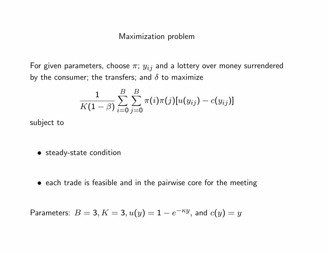
Maximization problem
For given parameters, choose π; yij and a lottery over money surrenderedby the consumer; the transfers; and δ to maximize
1
K(1− β)
B∑i=0
B∑j=0
π(i)π(j)[u(yij)− c(yij)]
subject to
• steady-state condition
• each trade is feasible and in the pairwise core for the meeting
Parameters: B = 3,K = 3, u(y) = 1− e−κy, and c(y) = y

Table 1. Optimal prob (%) of a unit transfer: the top number isfor those with 0 or 1, the bottom number is for those with 2
κ \ β .15 .2 .25 .3 .35 .4 .5 .6 .7 .8
2000
072
073
074
00
3.53.5
3.13.1
13.013.0
11.411.4
00
15 -00
065
067
067
00
00
5.35.3
2.82.8
00
12 - -00
059
061
00
00
2.12.1
00
00
10 - - -00
055
056
00
00
00
00
8 - - - -00
047
00
00
00
00
6 - - - - -00
038
00
00
00
5 - - - - - -00
00
00
00
4 - - - - - - -00.6
00
00
3 - - - - - - - -00.9
00

Lesson
Optimal policy is not simple
• even for this very simple model, the best policy is very dependent onthe parameters
The best policy ranges from paying substantial interest on large holdingsof money to giving lump-sum transfers– very different policies
• the former spreads out the distribution of money holdings, while thelatter compresses it

Coexistence of money and higher return assets
Hicks (1935): coexistence is the main challenge for monetary theory
• For Hicks, assuming a demand for money or putting money in theutility function are nonsenses
• Hicks proposed transaction costs (which we ought to regard as anothernonsense)
Cash-in-advance (CIA) did not exist when Hicks wrote
• Whether it gives rise to coexistence depends on your equilibrium notion

Individual defection or defection by the pair in each meeting
With individual defection, CIA is implementable
• each person choose from {yes, no} as response to a planner suggestedtrade
With defection by pairs, it, generally, is not
Tao Zhu and I (JET, 2007) took as our challenge getting coexistence whileallowing cooperative defection of the pair in each meeting

The partial equilibrium setting (strictly increasing and concavecontinuation value of nominal wealth)
Stage 1: portfolio choice
• government offers one-period discount bonds at a given price
• people with only money choose a portfolio
• (in the general equilibrium, interest is financed by money-creation)
Stage 2. Trejos-Wright (1995) with general portfolios of money and bonds

Stage-2 pairwise meetings
Bonds and money are perfect substitutes in terms of their payoffs at thestart of the next date
Therefore, pairwise-core outcomes are defined as a set of pairs: output ina meeting and the amount of wealth transferred
There are many pairwise-core outcomes: they range from giving all thegains-from-trade to the consumer to giving all to the producer
That allows us to reward buyers with a lot of money and, thereby, givespeople an incentive to leave stage-1 with some money

Comments
Role of pairwise trade (nondegenerate pairwise core)
Multiplicity (the favored assets could be money, bonds, or neither)
Welfare: can it be beneficial to have coexistence?
• Hu and Rocheteau (JET 2013)
— uses a version of Lagos-Wright (2005) with capital and money
— helps avoid over-accumulation of capital
• Hoonsik Yang (unpublished, part of his 2016 Ph.D. dissertation)
— works with examples in the Zhu-Wallace setting and the followingallowable portfolios: (0, 0), (1, 0), (2, 0) and (0, 1), (1, 1), (0, 2)

Cavalcanti and Wallace 1999
Maintain all of Trejos-Wright 1995 including {0, 1} money holdings, butassume
• some exogenous fraction of people are perfectly monitored, m-people;the rest, n-people, not monitored at all
— the endogenous state: the distribution of money between the twotypes
• the model was designed to compare inside (private) money and outsidemoney as alternative monetary systems
Here: two numerical examples, from joint work with Alexei Deviatov, thatuses an outside-money version to explore optimal policy

Monitoring and punishment
• ex ante identical people, but
— fraction α become permanently monitored (m-people)
— rest are permanently nonmonitored (n-people)
• for m-people, histories (and money holdings) are common knowledge
• for n-people, they are private
• monitored status and consumer/producer status are common knowl-edge
• only punishment is individual m→ n

Implementable stationary allocations
• state of economy: (θm, θn) ∈ [0, α]×[0, 1−α], fractions with money
• state of meeting: (s, s′) ∈ S × S, where S = {m,n} × {0, 1}
• a stationary allocation is (θm, θn), trades (including lotteries) in meet-ings, and transfers consistent with a steady state, a constant (θm, θn)
• a stationary allocation is implementable if
— trades are in the pairwise core and IC for n people
— transfers are IR and IC for n people

The planner
Choose a stationary and implementable allocation to maximize ex anteexpected utility before initial s is realized for each person
• ex ante expected utility is proportional to∑s∈S
∑s′∈S
πsπs′[u(yss′)− c(yss′)]
where yss′ is output in the (s, s′) meeting and
(πm1, πm0, πn1, πn0) = (θm, α− θm, θn, 1− α− θn)
• first-best is proportional to u(y∗)−c(y∗), where y∗ = argmax[u(y)−c(y)]

Example 1: Optimal inflation (Deviatov and Wallace 2010; workingpaper)
• inflation: a person who ends trade with money loses it with someprobability
• parameters: u(y) = 1−e−10y, c(y) = y,K = 3, β = .59, α = 1/4;
— arbitrary except for β; high enough so that if α = 1, thenmin{y, y∗} =y∗; low enough so that if α = 0, then optimal (y, θn)� (y∗, 1/2),where y is output in trade meetings
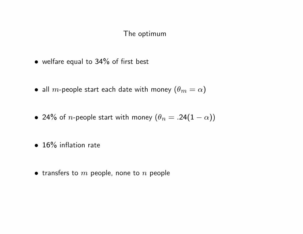
The optimum
• welfare equal to 34% of first best
• all m-people start each date with money (θm = α)
• 24% of n-people start with money (θn = .24(1− α))
• 16% inflation rate
• transfers to m people, none to n people

Table 1. Optimal trades(prod)(con) (output/y∗)/(money from consumer)(n0)(n1)* 0.57/(1)
(n0)(m1)* 0.57/(1)(m1)(n0) 0.11/(0)
(m1)(n1)* 0.38/(1)
(m1)(m1)* 0.38/(0)
More row-2 meetings than row-4 meetings (πn1 < πn0). Therefore,
• net inflow of money into holdings of n-people (more row-2 meetingsthan row-4 meetings)
• inflation and transfers to m-people (surprise?)

Similar inside-money result is in Deviatov and Wallace (RED 2014)
Inside money is different because money is issuer-specific
An m person defects without useful money
Transfers not needed, but the optimum has spending by m people thatexceeds earnings at each date, which produces inflation (surprise?)

Example 2. Optimal seasonal policy (Deviatov and Wallace JME 2009)
Same model except: a seasonal and zero average inflation is imposed
Parameters: α = 1/4, K = 3, u(y) = 2y1/2, β = .95, and
ct(y) =
{y/(0.80) if t is odd (winter)y/(1.25) if t is even (summer)
First date is odd (winter)
Implementable allocations: same except allowed to be two-date periodic
• If α = 1, then the first-best is implementable
• If α = 0, then the optimum is (yt, θnt) = (y∗t , 1/2) and welfare equalto 1/4 of first-best welfare


Table 2. Optimal quantity of money and welfarebeginning of winter beginning of summer
θm α αθn 0.312 0.309
welfare/first-best welfare .4558
there are no transfers to n-people
a higher quantity of money at beginning of winter
comparison to a no-intervention (constant money-supply) optimum
• no-intervention optimum also has θm = α at each date and, therefore,a constant θn and zero net flows between types at each date
• gain from intervention is about 1/2% in terms of consumption

Table 3. Optimal tradesmeeting (output/y∗t )/(money transferred)
(prod)(con) winter summer(n0)(n1) 0.95/(1.00) 0.95/(1.00)(n0)(m1) 0.85∗/(0.51) 0.78∗/(0.78)(m1)(n0) 0.16/(0) 0.17/(0)
(m1)(n1) 1.18†/(0.81) 0.84∗†/(1.00)(m1)(m1) 1.00/(0) 0.84∗/(0)
• net outflow from holdings of n people in winter, matching net inflowin summer
• m-people surrender money at beginning of summer and receive anexactly offsetting transfer at beginning of winter
— interpretation as planner loans: zero-interest loans to m-peopleat beginning of winter with repayment at beginning of summer(surprise and explanation?)
What can we learn from a few numerical examples?
They are consistent with the following related conclusions:
• if you know the model, then intervention is optimal
• even the qualitative nature of optimal intervention is not obvious
• optimal intervention depends on all the details
May need more examples to make those conclusions convincing

Concluding remarks
Somewhat standard view: judge a model not by the observations thatinspired it, but by its other implications that were not known when themodel was formulated. In that sense, the above applications are a tributeto the Shi and Trejos-Wright models.
Possible extensions:
• what if people in a meeting can hide assets
• nonstationary allocations and time consistent policy
• a large finite number of agents rather than a continuum