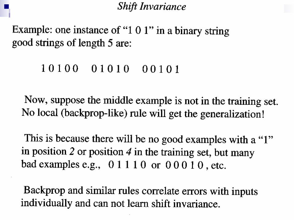
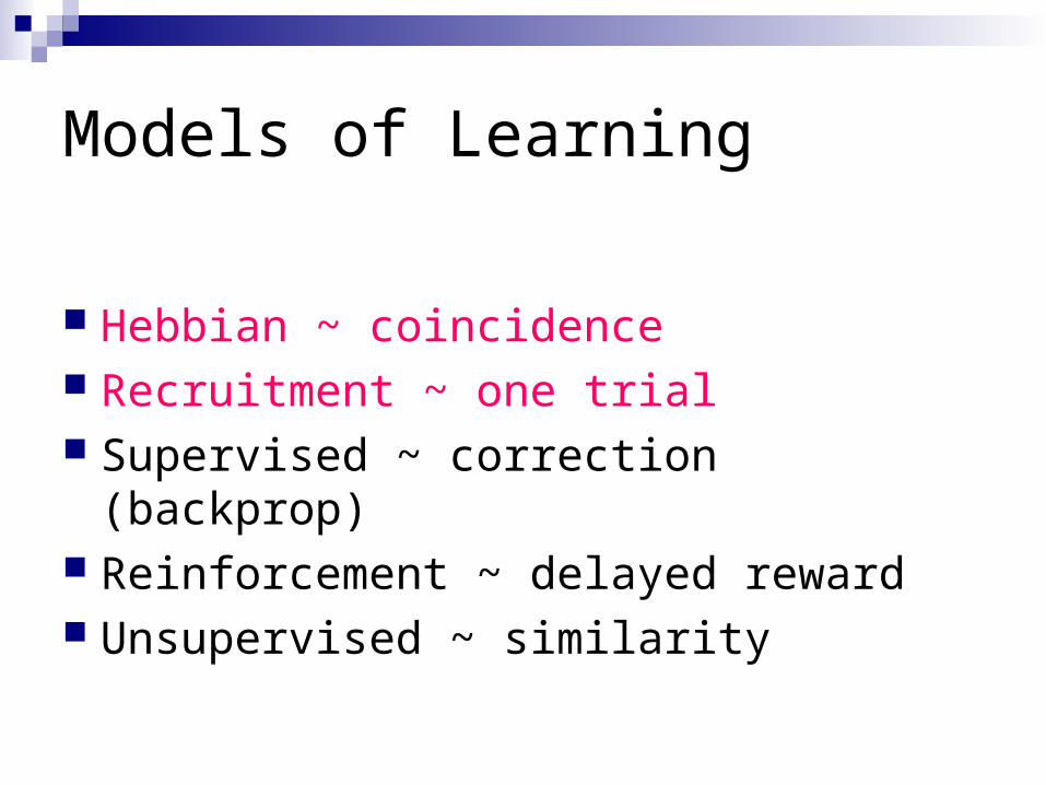
Models of Learning

Hebbian ~ coincidence Recruitment ~ one trial Supervised ~ correction (backprop) Reinforcement ~ delayed reward Unsupervised ~ similarity

Hebb’s Rule

The key idea underlying theories of neural learning go back to the Canadian psychologist Donald Hebb and is called Hebb’s rule.

From an information processing perspective, the goal of the system is to increase the strength of the neural connections that are effective.

Hebb (1949)

“When an axon of cell A is near enough to excite a cell B and repeatedly or persistently takes part in firing it, some growth process or metabolic change takes place in one or both cells such that A’s efficiency, as one of the cells firing B, is increased”From: The organization of behavior.

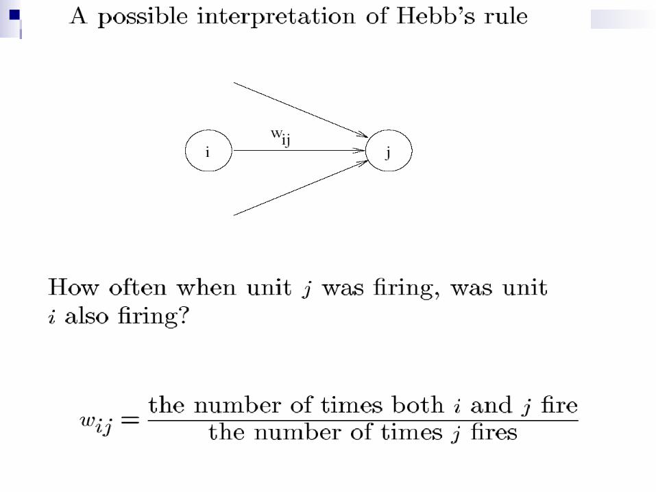
Hebb’s rule

Each time that a particular synaptic connection is active, see if the receiving cell also becomes active. If so, the connection contributed to the success (firing) of the receiving cell and should be strengthened. If the receiving cell was not active in this time period, our synapse did not contribute to the success the trend and should be weakened.

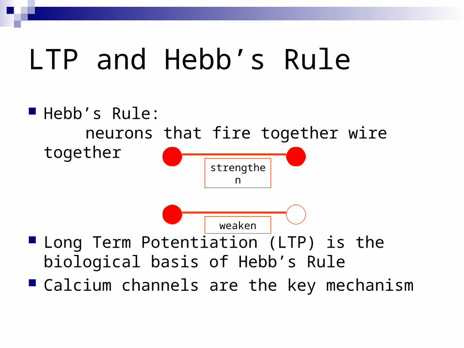
Hebb’s Rule: neurons that fire together wire together

Long Term Potentiation (LTP) is the biological basis of Hebb’s Rule

Calcium channels are the key mechanism

LTP and Hebb’s Rule

strengthen

weaken

Chemical realization of Hebb’s rule

It turns out that there are elegant chemical processes that realize Hebbian learning at two distinct time scales

Early Long Term Potentiation (LTP) Late LTP

These provide the temporal and structural bridge from short term electrical activity, through intermediate memory, to long term structural changes.

Calcium Channels Facilitate Learning In addition to the synaptic channels responsible

for neural signaling, there are also Calcium-based channels that facilitate learning. As Hebb suggested, when a receiving neuron fires,

chemical changes take place at each synapse that was active shortly before the event.

Long Term Potentiation (LTP)

These changes make each of the winning synapses more potent for an intermediate period, lasting from hours to days (LTP).

In addition, repetition of a pattern of successful firing triggers additional chemical changes that lead, in time, to an increase in the number of receptor channels associated with successful synapses - the requisite structural change for long term memory. There are also related processes for weakening synapses and

also for strengthening pairs of synapses that are active at about the same time.

The Hebb rule is found with long term potentiation (LTP) in the hippocampus

1 sec. stimuliAt 100 hz

Schafer collateral pathwayPyramidal cells

With high-frequency stimulation, Calcium comes in

During normal low-frequency trans-mission, glutamate interacts with NMDA and non-NMDA (AMPA) and metabotropic receptors.

Enhanced Transmitter Release

AMPA

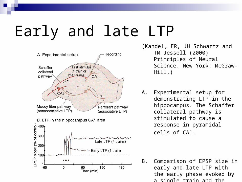
Early and late LTP (Kandel, ER, JH Schwartz and TM Jessell

(2000) Principles of Neural Science. New York: McGraw-Hill.)

A. Experimental setup for demonstrating LTP in the hippocampus. The Schaffer collateral pathway is stimulated to cause a response in pyramidal cells of

CA1.

B. Comparison of EPSP size in early and late LTP with the early phase evoked by a single train and the late phase by 4

trains of pulses.

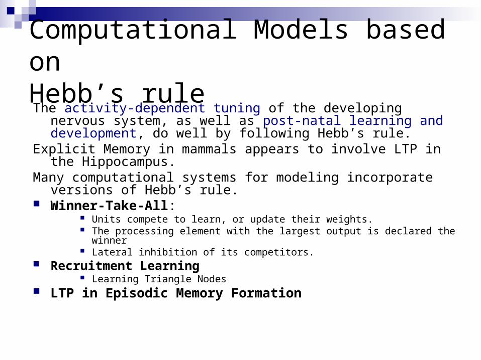
Computational Models based onHebb’s ruleThe activity-dependent tuning of the developing nervous system, as

well as post-natal learning and development, do well by following Hebb’s rule.

Explicit Memory in mammals appears to involve LTP in the Hippocampus.

Many computational systems for modeling incorporate versions of Hebb’s rule.

Winner-Take-All: Units compete to learn, or update their weights. The processing element with the largest output is declared the winner Lateral inhibition of its competitors.

Recruitment Learning Learning Triangle Nodes

LTP in Episodic Memory Formation

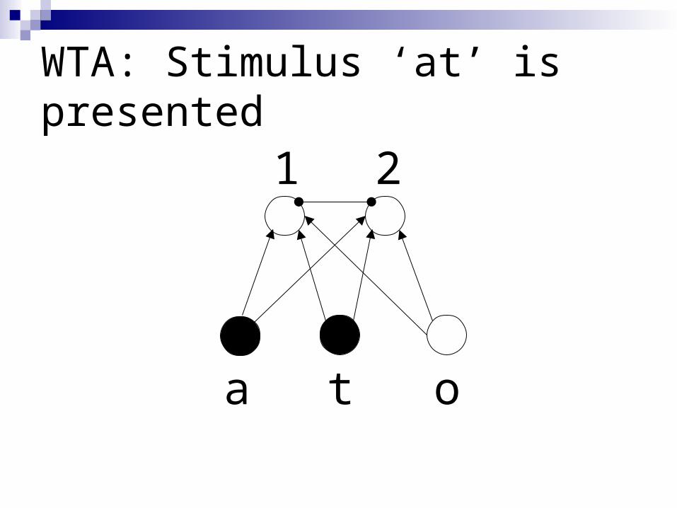
WTA: Stimulus ‘at’ is presented

a t o

1 2

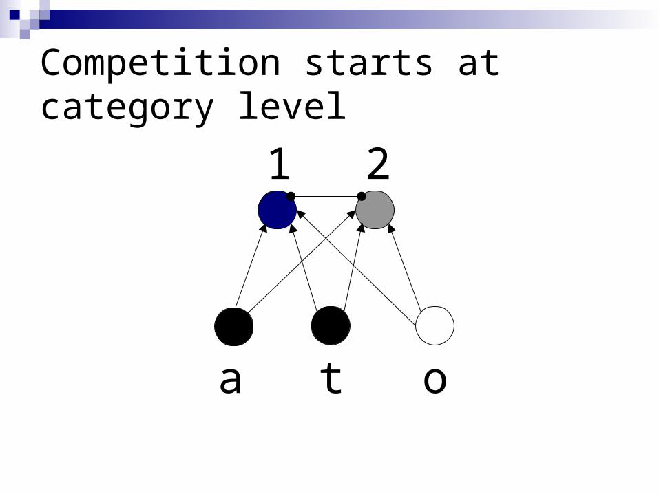
Competition starts at category level

a t o

1 2

Competition resolves

a t o

1 2

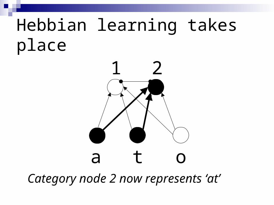
Hebbian learning takes place

a t o

1 2

Category node 2 now represents ‘at’

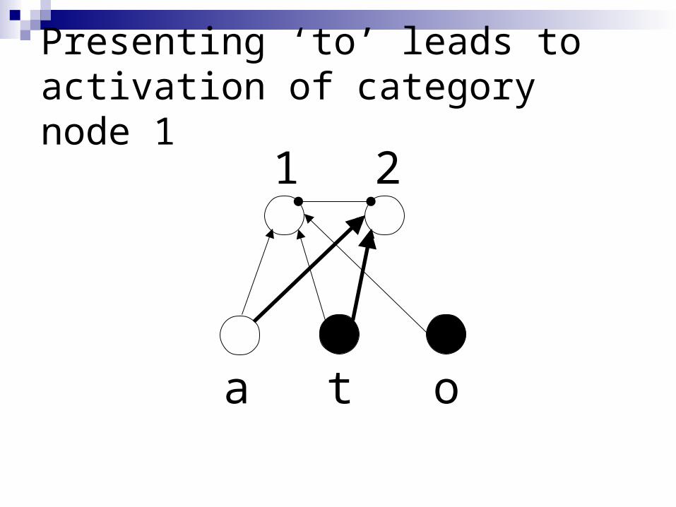
Presenting ‘to’ leads to activation of category node 1

a t o

1 2

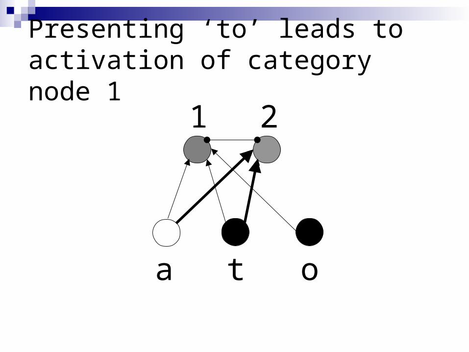
Presenting ‘to’ leads to activation of category node 1

a t o

1 2

Presenting ‘to’ leads to activation of category node 1

a t o

1 2

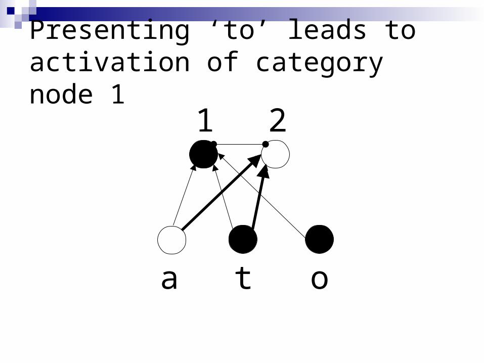
Presenting ‘to’ leads to activation of category node 1

a t o

1 2

Category 1 is established through Hebbian learning as well

a t o

1 2

Category node 1 now represents ‘to’

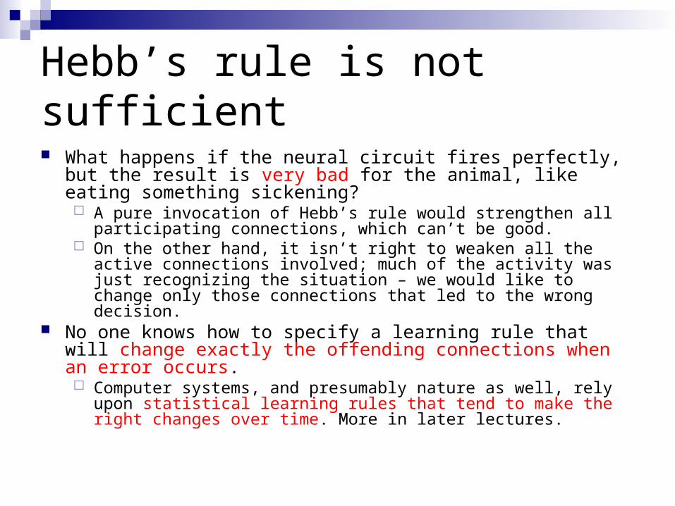
Hebb’s rule is not sufficient

What happens if the neural circuit fires perfectly, but the result is very bad for the animal, like eating something sickening? A pure invocation of Hebb’s rule would strengthen all participating

connections, which can’t be good. On the other hand, it isn’t right to weaken all the active connections

involved; much of the activity was just recognizing the situation – we would like to change only those connections that led to the wrong decision.

No one knows how to specify a learning rule that will change exactly the offending connections when an error occurs. Computer systems, and presumably nature as well, rely upon statistical

learning rules that tend to make the right changes over time. More in later lectures.

Hebb’s rule is insufficient

should you “punish” all the connections?

tastebud tastes rotten eats food gets sick

drinks water

Models of Learning

Hebbian ~ coincidence Recruitment ~ one trial Supervised ~ correction (backprop) Reinforcement ~ delayed reward Unsupervised ~ similarity

Recruiting connections

Given that LTP involves synaptic strength changes and Hebb’s rule involves coincident-activation based strengthening of connectionsHow can connections between two nodes be

recruited using Hebbs’s rule?

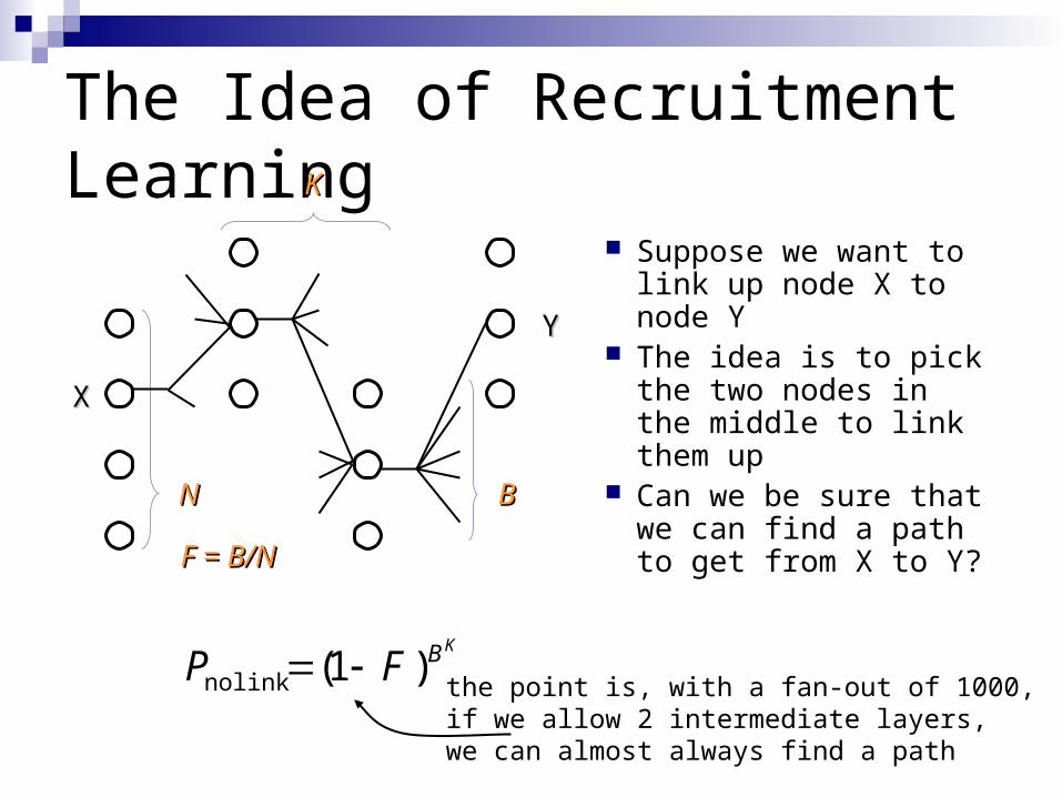
The Idea of Recruitment Learning

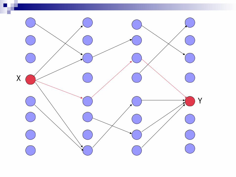
Suppose we want to link up node X to node Y

The idea is to pick the two nodes in the middle to link them up

Can we be sure that we can find a path to get from X to Y?

KBFP )1(link no the point is, with a fan-out of 1000, if we allow 2 intermediate layers, we can almost always find a path

XX

YY

BBNN

KK

F = B/NF = B/N

X

Y

X

Y

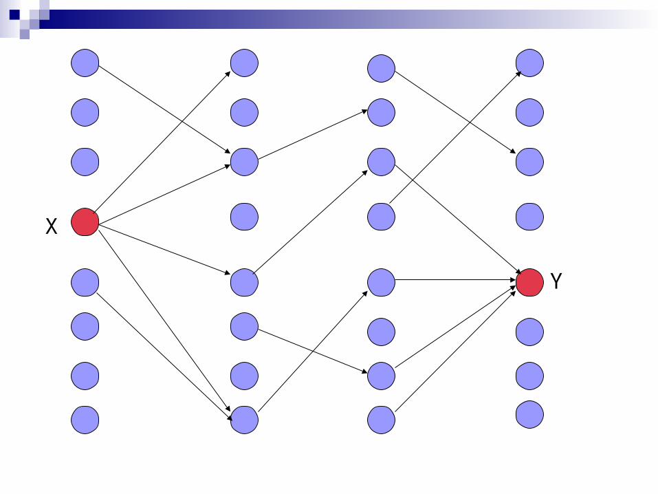
Finding a Connection

P = Probability of NO link between X and Y

N = Number of units in a “layer”

B = Number of randomly outgoing units per unit

F = B/N , the branching factor

K = Number of Intermediate layers, 2 in the example

0 .999 .9999 .99999

1 .367 .905 .989

2 10-440 10-44 10-5

N=K=

# Paths = (1-P k-1)*(N/F) = (1-P k-1)*B

P = (1-F) **B**K

106 107 108

Finding a Connection in Random Networks

For Networks with N nodes and branching factor,

there is a high probability of finding good links.

(Valiant 1995)

N

Recruiting a Connection in Random Networks

Informal Algorithm

1. Activate the two nodes to be linked

2. Have nodes with double activation strengthen their active synapses (Hebb)

3. There is evidence for a “now print” signal based on LTP (episodic memory)

Triangle nodes and feature structures

B C

A

A B C

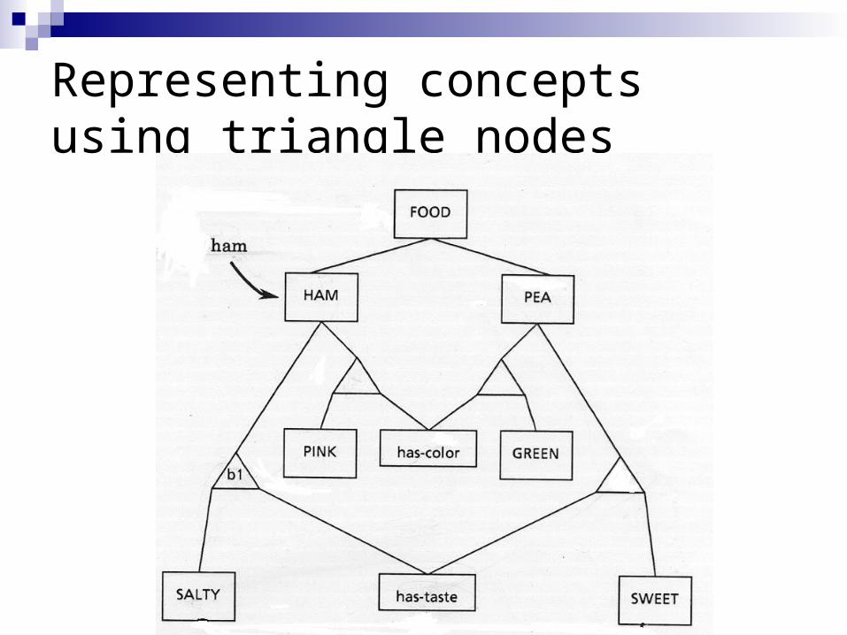
Representing concepts using triangle nodes

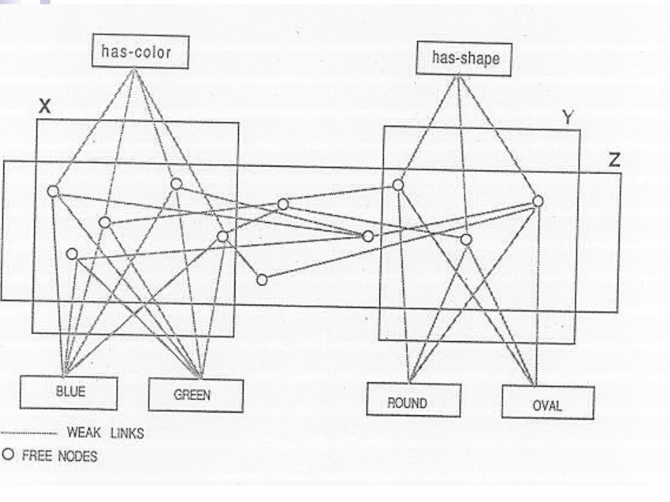
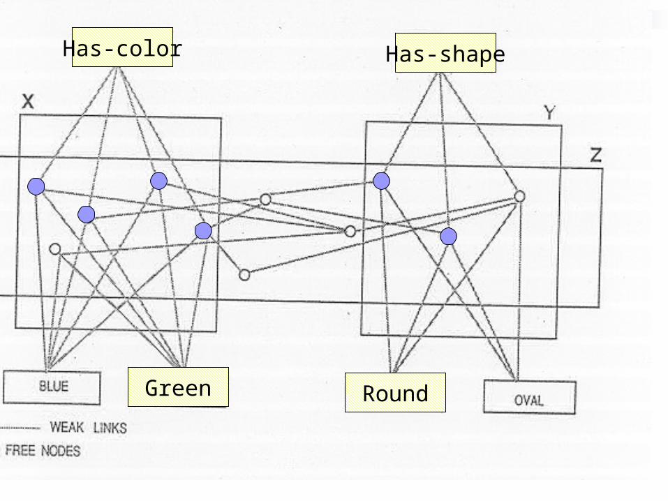
Recruiting triangle nodes Let’s say we are trying to remember a green circle currently weak connections between concepts (dotted lines)

has-color

blue green round oval

has-shape

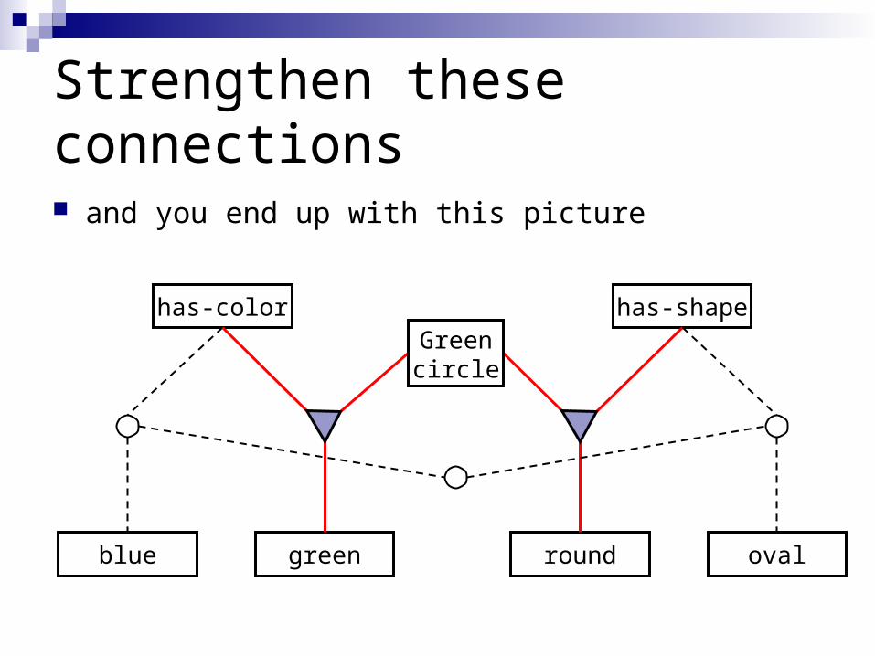
Strengthen these connections

and you end up with this picture

has-color

blue green round oval

has-shapeGreencircle

Has-color

Green

Has-shape

Round

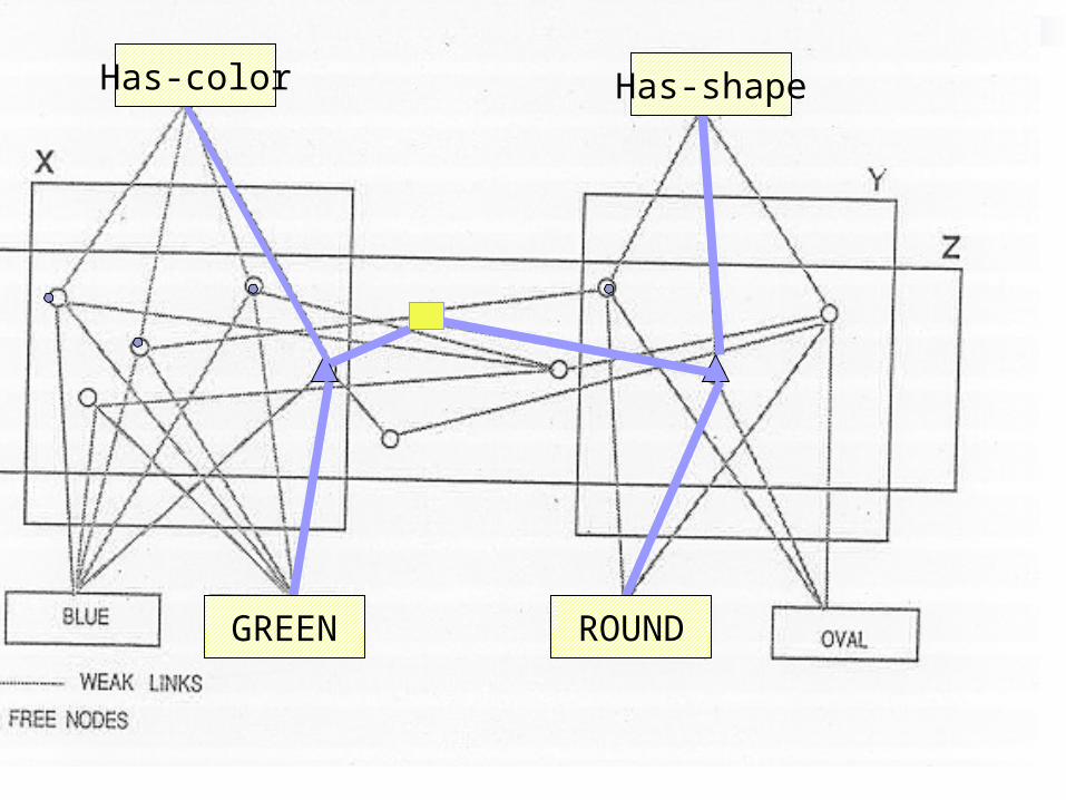
Has-color Has-shape

GREEN ROUND

Back Propagation

Jerome FeldmanCS182/CogSci110/Ling109Spring 2007

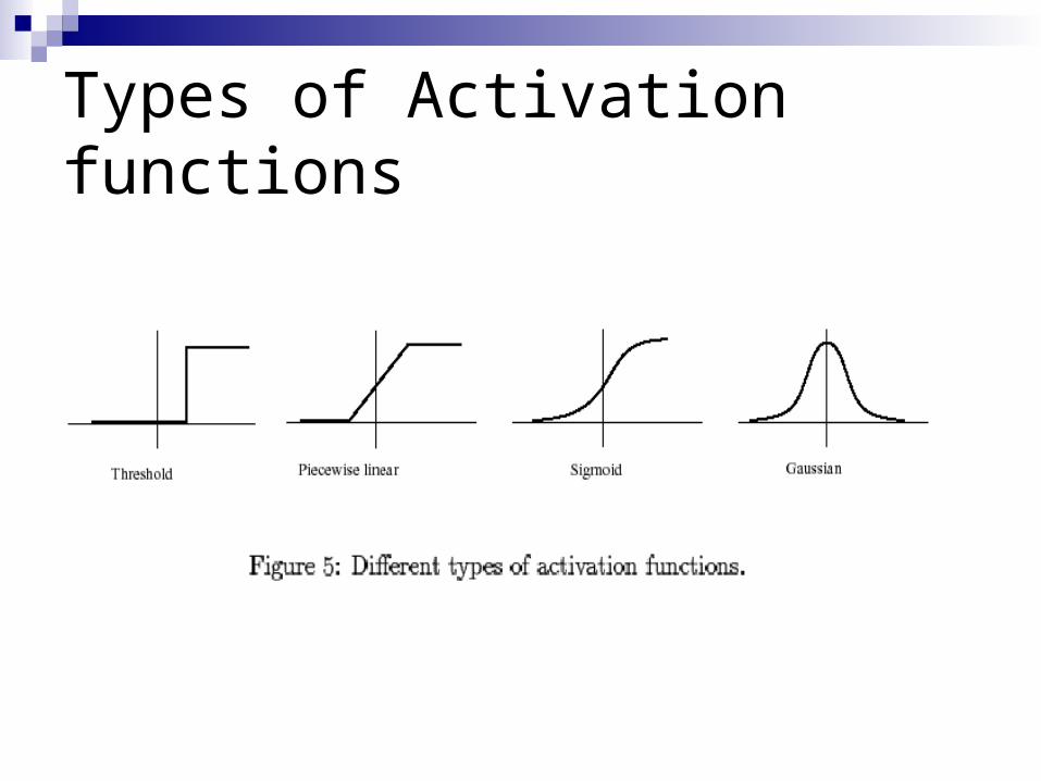
Types of Activation functions

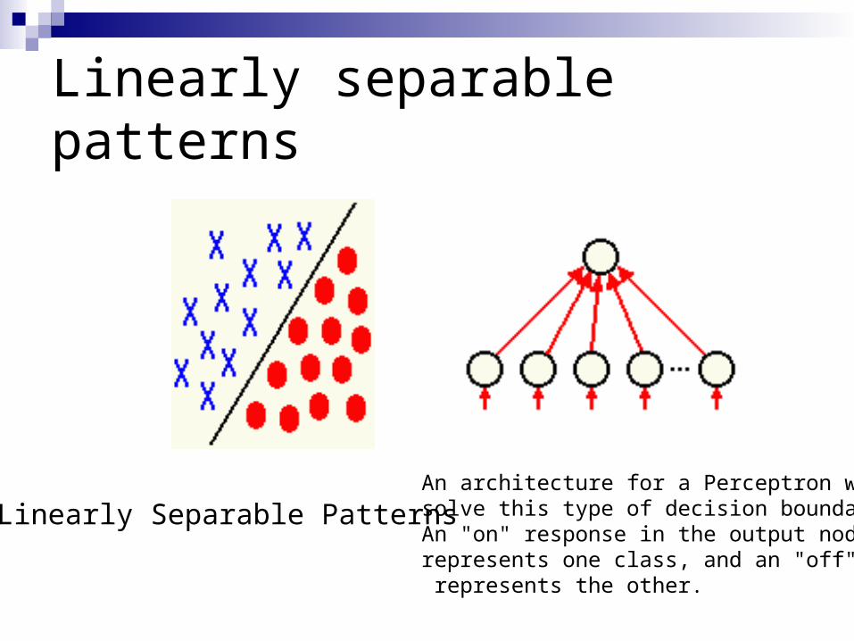
Linearly separable patterns

Linearly Separable PatternsAn architecture for a Perceptron which can solve this type of decision boundary problem. An "on" response in the output node represents one class, and an "off" response represents the other.

Multi-layer Feed-forward Network

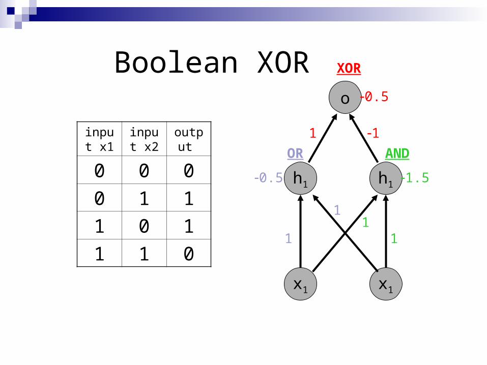
Boolean XOR

input x1

input x2

output

0 0 0

0 1 1

1 0 1

1 1 0

h1

x1

o

x1

h1

1

1.5

AND

11

0.5

OR

1

1

0.5

XOR

1

Pattern Separation and NN architecture

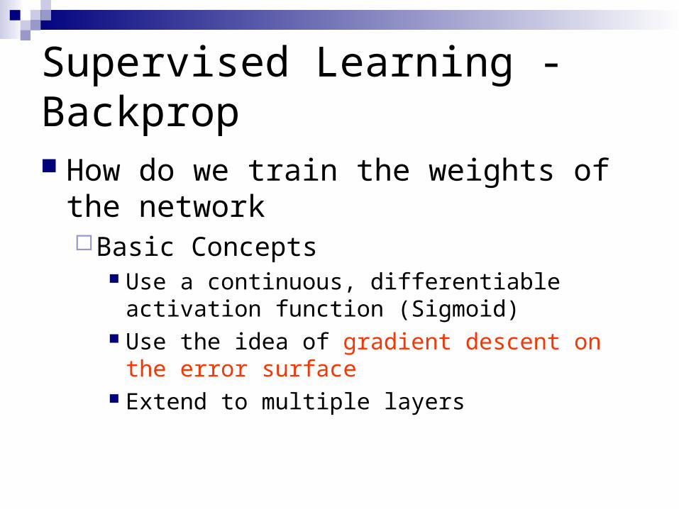
Supervised Learning - Backprop

How do we train the weights of the networkBasic Concepts

Use a continuous, differentiable activation function (Sigmoid)

Use the idea of gradient descent on the error surface

Extend to multiple layers

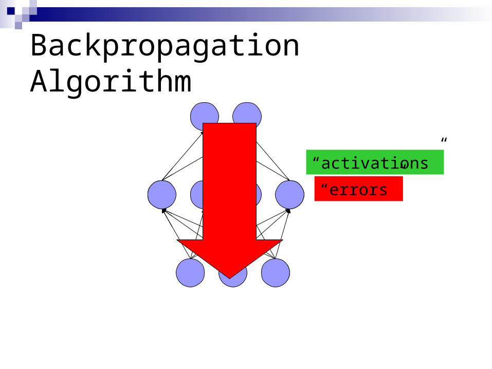
Backpropagation Algorithm

“activations”

“errors”

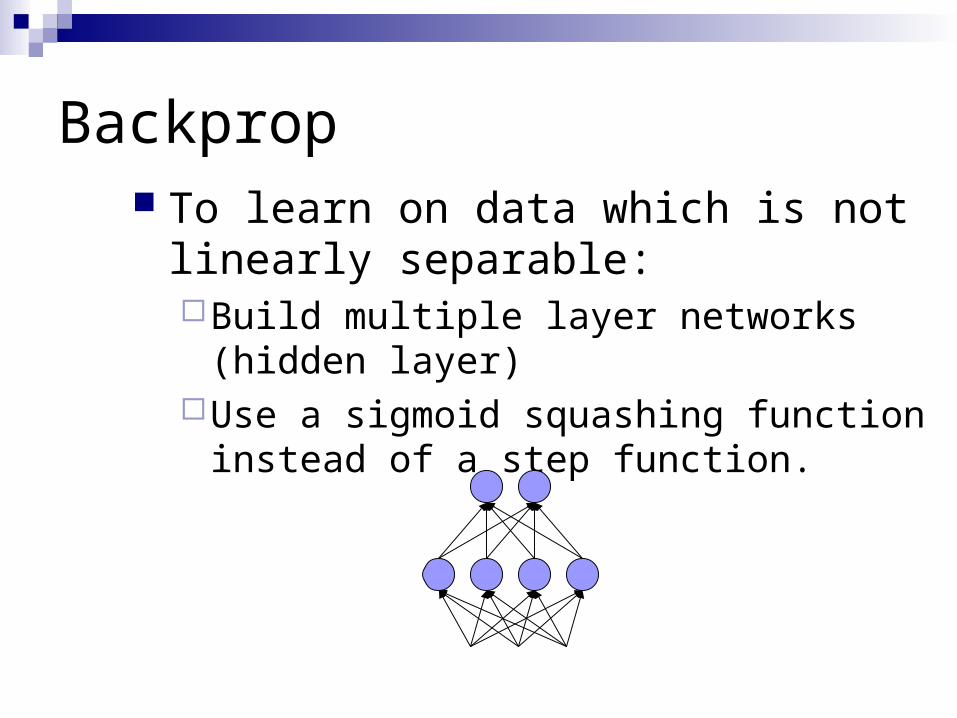
Backprop To learn on data which is not linearly

separable:Build multiple layer networks (hidden layer)Use a sigmoid squashing function instead

of a step function.

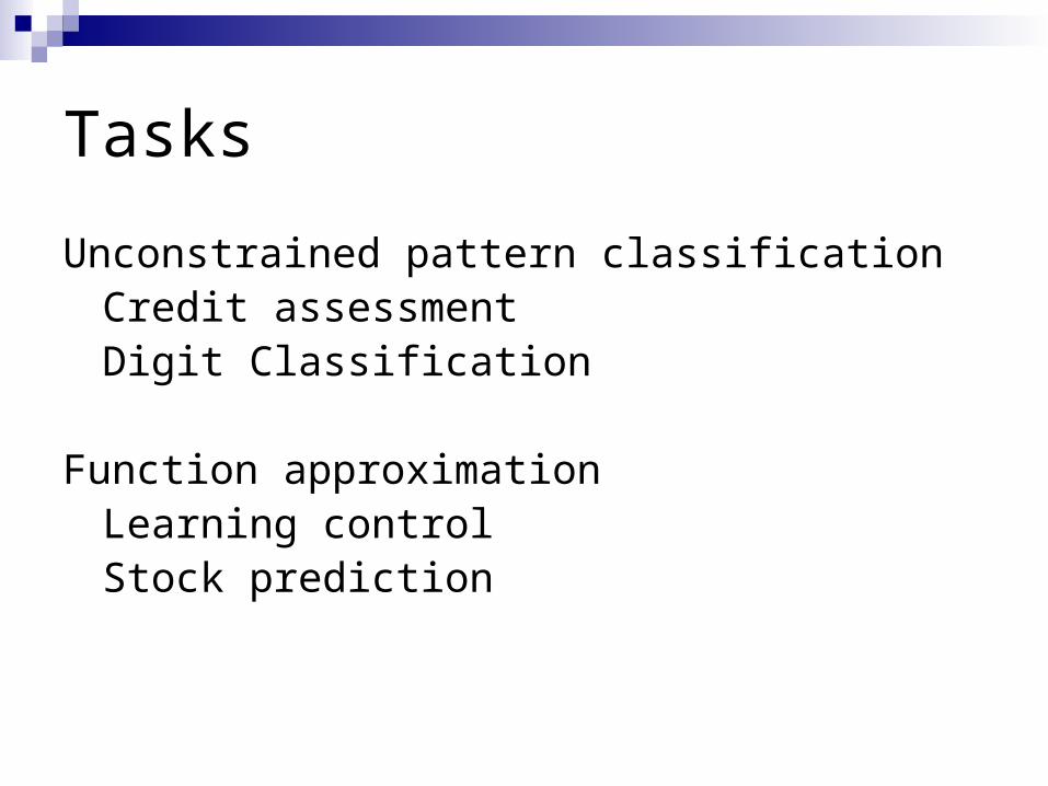
Tasks

Unconstrained pattern classificationCredit assessmentDigit Classification

Function approximationLearning controlStock prediction

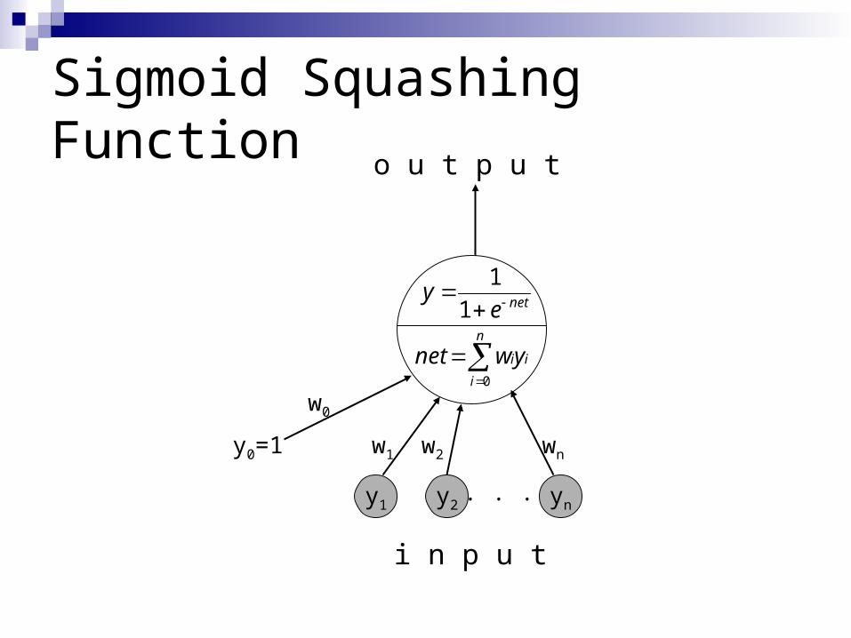
Sigmoid Squashing Function

w2 wnw1

w0

y0=1

o u t p u t

y2 yny1. . .

i n p u t

n

i

iiywnet0

netey

1

1

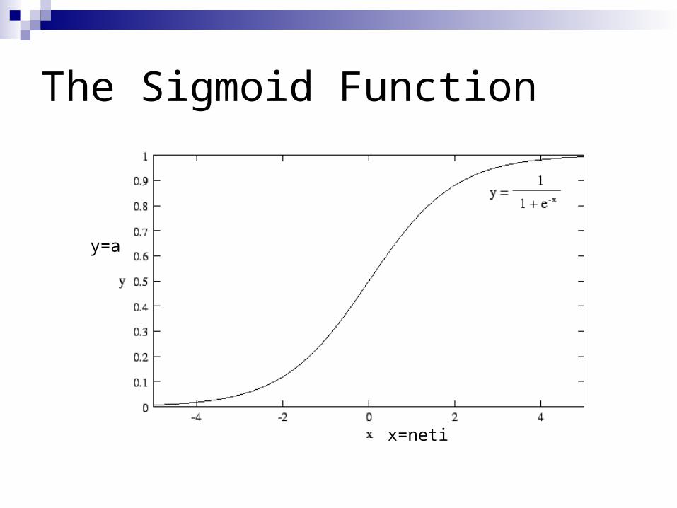
The Sigmoid Function

x=neti

y=a

Nice Property of Sigmoids

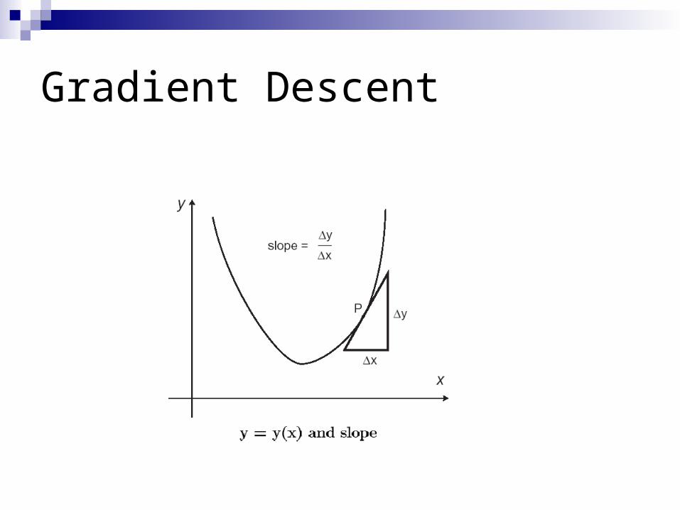
Gradient Descent

Gradient Descent on an error

Learning Rule – Gradient Descent on an Root Mean Square (RMS)

Learn wi’s that minimize squared error

21[ ] ( )

2 k kk O

E w t o

O = output layer

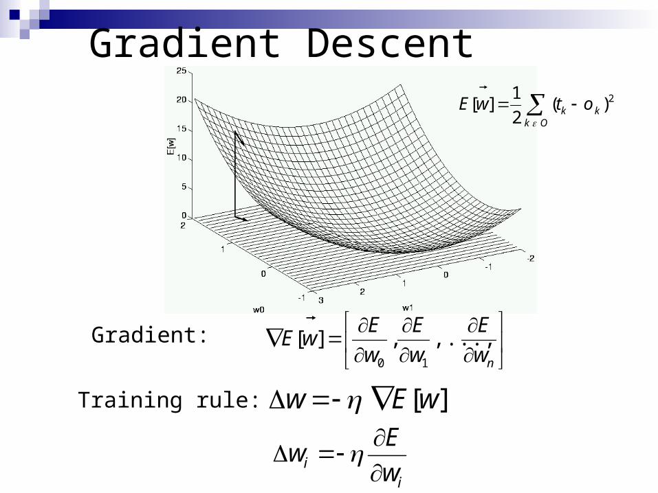
Gradient Descent

Gradient:

nw

E

w

E

w

EwE ,...,,][

10

ii w

Ew

Training rule: ][wEw

21[ ] ( )

2 k kk O

E w t o

Backpropagation Algorithm

Generalization to multiple layers and multiple output units

An informal account of BackProp

For each pattern in the training set:

Compute the error at the output nodes

Compute w for each wt in 2nd layer

Compute delta (generalized error expression) for hidden units

Compute w for each wt in 1st layer

After amassing w for all weights and, change each wt a little bit, as determined by the learning rate

jpipij ow

Backprop Details

Here we go…

Also refer to web notes for derivation

k j i

wjk wij

E = Error = ½ ∑i (ti – yi)2

yi

ti: targetij

ijij W

EWW

ijij W

EW

jiiiij

i

i

i

iij

yxfytW

x

x

y

y

E

W

E

)('

The derivative of the sigmoid is just ii yy 1

jiiiiij yyyytW 1

ijij yW iiiii yyyt 1

The output layerlearning rate

k j i

wjk wij

E = Error = ½ ∑i (ti – yi)2

yi

ti: target

The hidden layerjk

jk W

EW

jk

j

j

j

jjk W

x

x

y

y

E

W

E

iijiii

i j

i

i

i

ij

Wxfyty

x

x

y

y

E

y

E)(')(

kji

ijiiijk

yxfWxfytW

E

)(')(')(

kjji

ijiiiijk yyyWyyytW

11)(

jkjk yW jji

ijiiiij yyWyyyt

11)(

jji

iijj yyW

1

Let’s just do an example

E = Error = ½ ∑i (ti – yi)2x0 f

i1 w01

y0i2

b=1

w02

w0b

E = ½ (t0 – y0)2

i1 i2 y0

0 0 0

0 1 1

1 0 1

1 1 10.8

0.6

0.5

0

00.6224

0.51/(1+e^-0.5)

E = ½ (0 – 0.6224)2 = 0.1937

ijij yW iiiii yyyt 1

01 i 0

0

00000 1 yyyt

6224.016224.06224.000

1463.00

1463.0

0101 yW

0202 yW

00 bb yW

02 i

0 b

learning rate

suppose = 0.50731.01463.05.00 bW

0.4268

Momentum term

The speed of learning is governed by the learning rate. If the rate is low, convergence is slow If the rate is too high, error oscillates without reaching minimum.

Momentum tends to smooth small weight error fluctuations.

n)(n)y()1n(ij

wn)(ij

w ji

10

the momentum accelerates the descent in steady downhill directions.the momentum has a stabilizing effect in directions that oscillate in time.

Convergence

May get stuck in local minima Weights may diverge

…but works well in practice

Representation power:2 layer networks : any continuous function3 layer networks : any function

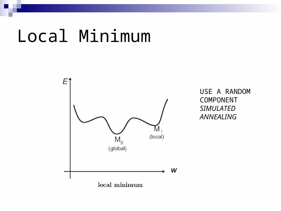
Local Minimum

USE A RANDOM COMPONENT SIMULATED ANNEALING

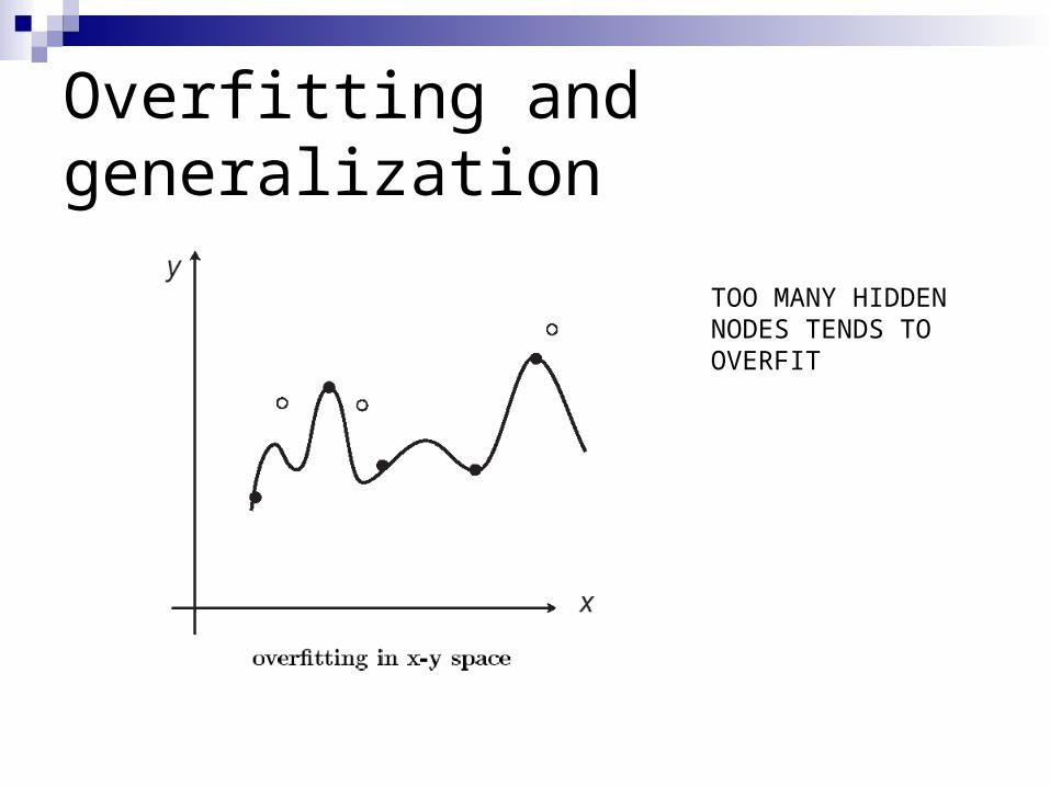
Overfitting and generalization

TOO MANY HIDDEN NODES TENDS TO OVERFIT

Overfitting in ANNs

Early Stopping (Important!!!)

Stop training when error goes up on validation set

Stopping criteria

Sensible stopping criteria: total mean squared error change:

Back-prop is considered to have converged when the absolute rate of change in the average squared error per epoch is sufficiently small (in the range [0.01, 0.1]).

generalization based criterion: After each epoch the NN is tested for generalization. If the generalization performance is adequate then stop. If this stopping criterion is used then the part of the training set used for testing the network generalization will not be used for updating the weights.

Architectural ConsiderationsWhat is the right size network for a given job?

How many hidden units?

Too many: no generalization

Too few: no solution

Possible answer: Constructive algorithm, e.g.

Cascade Correlation (Fahlman, & Lebiere 1990)

etc

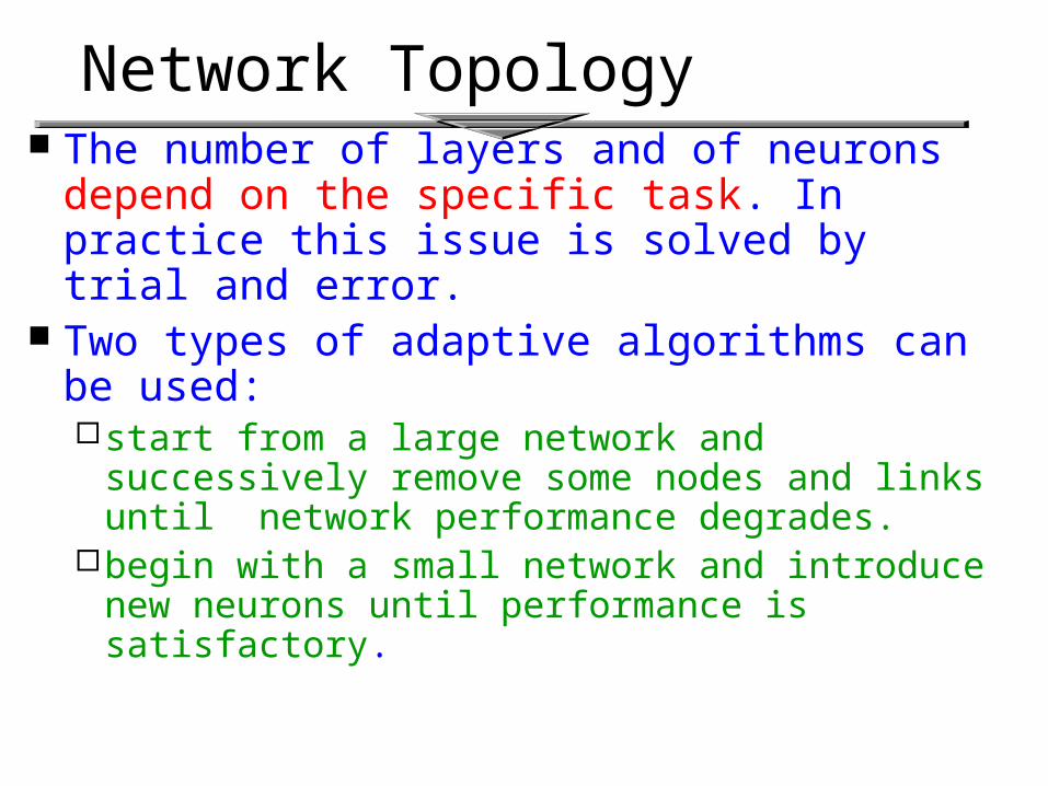
The number of layers and of neurons depend on the specific task. In practice this issue is solved by trial and error.

Two types of adaptive algorithms can be used:start from a large network and successively

remove some nodes and links until network performance degrades.

begin with a small network and introduce new neurons until performance is satisfactory.

Network Topology

Supervised vs Unsupervised Learning

•Backprop requires a 'target'

•how realistic is that?

•Hebbian learning is unsupervised, but limited in power

•How can we combine the power of backprop (and friends) with the ideal of unsupervised learning?

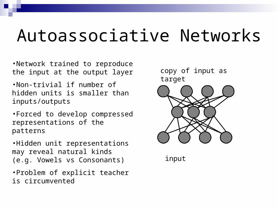
Autoassociative Networks

input

copy of input as target

•Network trained to reproduce the input at the output layer

•Non-trivial if number of hidden units is smaller than inputs/outputs

•Forced to develop compressed representations of the patterns

•Hidden unit representations may reveal natural kinds (e.g. Vowels vs Consonants)

•Problem of explicit teacher is circumvented

Problems and Networks

•Some problems have natural "good" solutions

•Solving a problem may be possible by providing the right armory of general-purpose tools, and recruiting them as needed

•Networks are general purpose tools.

•Choice of network type, training, architecture, etc greatly influences the chances of successfully solving a problem

•Tension: Tailoring tools for a specific job Vs Exploiting general purpose learning mechanism

Summary

Multiple layer feed-forward networksReplace Step with Sigmoid (differentiable)

function Learn weights by gradient descent on error

functionBackpropagation algorithm for learningAvoid overfitting by early stopping

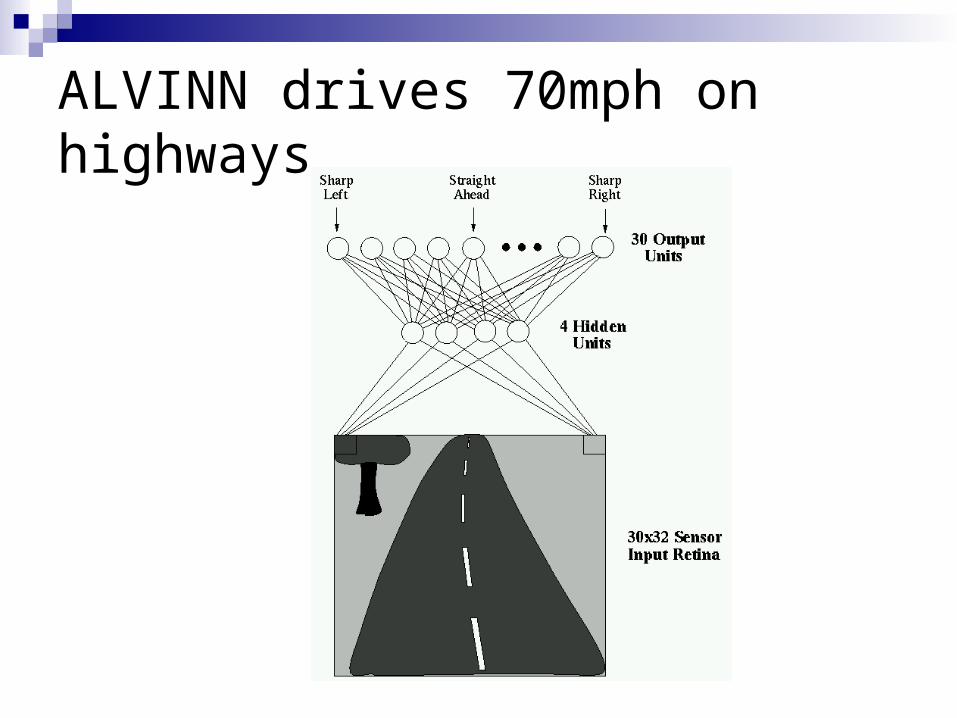
ALVINN drives 70mph on highways

Use MLP Neural Networks when …

(vectored) Real inputs, (vectored) real outputs

You’re not interested in understanding how it works

Long training times acceptable Short execution (prediction) times required Robust to noise in the dataset

Applications of FFNNClassification, pattern recognition: FFNN can be applied to tackle non-linearly separable

learning problems. Recognizing printed or handwritten characters, Face recognition Classification of loan applications into credit-worthy and non-

credit-worthy groups Analysis of sonar radar to determine the nature of the source

of a signal

Regression and forecasting: FFNN can be applied to learn non-linear functions

(regression) and in particular functions whose inputs is a sequence of measurements over time (time series).

Extensions of Backprop Nets

Recurrent Architectures Backprop through time

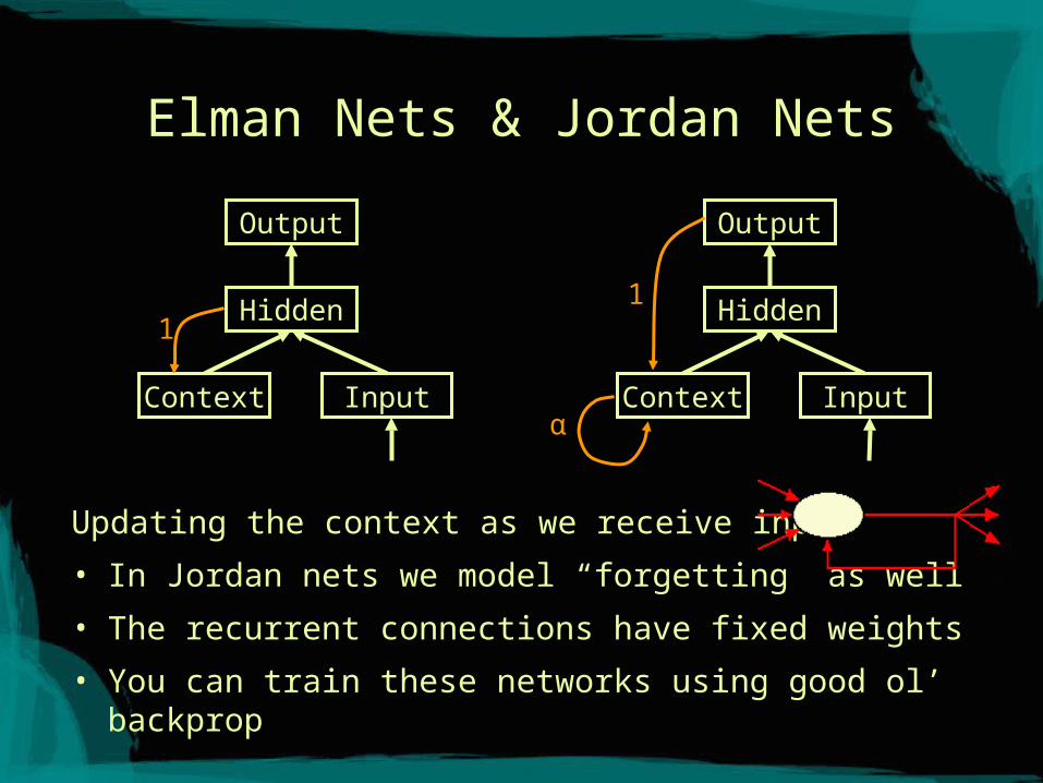
Elman Nets & Jordan Nets

Updating the context as we receive input

• In Jordan nets we model “forgetting” as well

• The recurrent connections have fixed weights

• You can train these networks using good ol’ backprop

Output

Hidden

Context Input

1

α

Output

Hidden

Context Input

1

Recurrent Backprop

• we’ll pretend to step through the network one iteration at a time

• backprop as usual, but average equivalent weights (e.g. all 3 highlighted edges on the right are equivalent)

a b c unrolling3 iterations

a b c

a b c

a b cw2

w1 w3

w4

w1 w2 w3 w4

a b c