HAL Id: hal-01263932https://hal-mines-paristech.archives-ouvertes.fr/hal-01263932

Submitted on 28 Jan 2016

HAL is a multi-disciplinary open accessarchive for the deposit and dissemination of sci-entific research documents, whether they are pub-lished or not. The documents may come fromteaching and research institutions in France orabroad, or from public or private research centers.

L’archive ouverte pluridisciplinaire HAL, estdestinée au dépôt et à la diffusion de documentsscientifiques de niveau recherche, publiés ou non,émanant des établissements d’enseignement et derecherche français ou étrangers, des laboratoirespublics ou privés.

Modelling the microstructure and the viscoelasticbehaviour of carbon black filled rubber materials from

3D simulationsBruno Figliuzzi, Dominique Jeulin, Matthieu Faessel, François Willot,

Masataka Koishi, Naoya Kowatari

To cite this version:Bruno Figliuzzi, Dominique Jeulin, Matthieu Faessel, François Willot, Masataka Koishi, et al.. Mod-elling the microstructure and the viscoelastic behaviour of carbon black filled rubber materials from3D simulations. Technische Mechanik, Magdeburger Verein für Technische Mechanik e.V., 2016, 32(1-2), pp.22-46. hal-01263932

Modelling the microstructure and the viscoelastic behaviour ofcarbon black filled rubber materials from 3D Simulations

B. Figliuzzi1, D. Jeulin1, M. Faessel1, F. Willot1, M. Koishi2, N. Kowatari2

1 Mines ParisTech, PSL Research University, 35 rue Saint Honore F-77305 Fontainebleau Cedex, France2 KOISHI Lab. R and D Center The Yokohama Rubber Co., Ltd. 2-1 Oiwake, Hiratsuka Kanagawa 254-8601,Japan

Published in: Technische Mechanik 32(1–2), 22–46 (2016). “Postprint” version with larger figures, text

and results unchanged.

Volume fraction and spatial repartition of fillers impact the physical properties of rubber. Extended percolatingnetworks of nano-sized fillers significantly modify the macroscopic mechanical properties of rubbers. Randommodels that describe the multiscale microstructure of rubber and efficient Fourier-based numerical algorithms arecombined to predict the material’s mechanical properties. From TEM image analysis, various types of multiscalemodels were proposed and validated, accounting for the non-homogeneous distribution of fillers: in the presentwork, aggregates are located outside of an exclusion polymer simulated by two families of random models. Thefirst model generates the exclusion polymer by a Boolean model of spheres. In the second model, the exclusionpolymer is a mosaic model built from a Johnson-Mehl tessellation. Here the exclusion polymer and the polymercontaining the filler show a similar morphology, contrary to the Boolean model. Aggregates are then describedas the intersection of a Boolean model of spheres and of the complementary of the exclusion polymer. Carbonblack particles are simulated by a Cox model of spheres in the aggregates. The models rely on a limited numberof parameters fitted from experimental covariance and cumulative granulometry. The influence of the modelparameters on percolation properties of the models is studied numerically from 3D simulations. Finally, a novelFourier-based algorithm is proposed to estimate the viscoelastic properties of linear heterogeneous media, in theharmonic regime. The method is compared to analytical results and to a different, time-discretized FFT scheme.As shown in this work, the proposed numerical method is efficient for computing the viscoelastic response ofmicrostructures containing rubbers and fillers.

1 Introduction

Mechanical properties of rubbers are often improved by including nanoscopic fillers in their composition. Usually,silica and carbon black materials are used for this purpose. The geometrical properties of the fillers are animportant feature of the global material. In particular, their volume fraction and spatial distribution largelydetermine the physical properties of the rubber. Extended percolating networks of fillers can for instancesignificantly enhance the mechanical properties of rubbers on macroscopic scales.

This work investigates the influence of the fillers geometry on the viscoelastic properties of rubber. Animportant step toward the completion of this research is the development of random models describing theircomplex microstructure. Following a now well-established method in material science as in [15], random real-izations of these models can in turn be used to perform an extensive study of the mechanical properties of therubber.

As reviewed by [13], several models have been developed in the past 20 years to describe the microstructureof rubbers. [3] developed a model describing the carbon aggregates as squares or dodecahedra in an elastomericvolume. Even if their model only accounts for the scale of aggregates, they were able to conduct extensivefinite elements calculations aimed at describing the large deformation behavior of the rubber. Relying on asimilar approach, [19] developed a cuberbille model to describe carbon aggregates in a rubber matrix. In theirmodel, they notably added a third phase accounting for a layer of bound rubber surrounding the aggregates.[32] improved the microstructure description by considering that aggregates can be represented as the union ofcarbon black spherical-shaped particles, eventually opening the way to the development of more accurate models.Carbon black composites have finally been widely investigated at the Center for Mathematical Morphologyby [18], [34], [7] and [30].

In this paper, we first introduce the studied material nanostructure from TEM micrographs. After a morpho-logical segmentation of images, measurements are performed to quantitatively characterize the microstructure.Then, two random set models to reproduce the multiscale microstructure of rubbers are developed. They areidentified from the available experimental data obtained on TEM images and on simulations. In Section 4, wefocus on the issue of percolation, which is of particular interest regarding the microstructure optimization. In the

1

last part, viscoelastic properties of the material are predicted by means of Fast Fourier Transforms performedon simulated 3D images generated from the random model.

2 TEM Images analysis

2.1 Material

This work concerns a rubber material reinforced by carbon black particles as fillers, that are embedded in amatrix of rubber and can be geometrically well-approximated by spheres of diameter D ' 30 − 40 nm, asillustrated in Figure 1a. The volume fraction of the fillers is around 14 percents in the rubber. A key featureof the material is that the rubber matrix is constituted of two distinct polymers: an exclusion polymer, whichcannot contain any filler, and its complementary polymer, which can contain fillers. Fillers tend to agglomeratetogether within the rubber matrix. The filler particles indeed exhibit a turbostratic structure which enablethem to merge and create aggregates [13].

2.2 TEM images segmentation

To analyze the rubbers microstructure, we dispose of a set of 50 TEM micrographs of size 1024 by 1024 pixelswith resolution 2.13 nm per pixel. These images were obtained in the Yokohama Rubber Research Center. Theslices of material probed by the microscope have a thickness around 40 nm. The first task is to segment theseimages, in order to identify the spatial distribution of the fillers. The segmentation procedure and its results arepresented in the first two paragraphs of this section. The next step is to extract morphological characteristicsfrom the segmented TEM images, as described in the third paragraph.

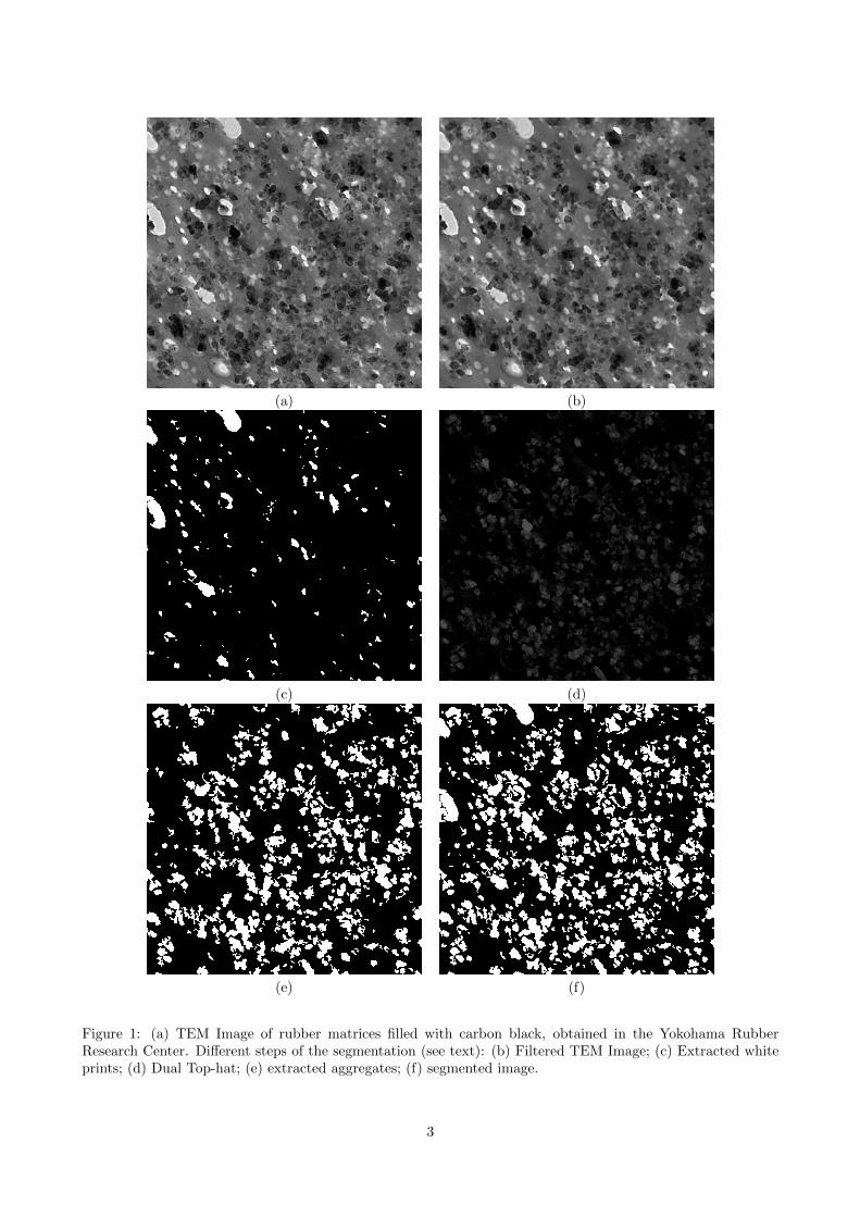
Algorithm The segmentation process aims at extracting the carbon black phase from the 8 bits TEM images.White regions can be observed in the images, which correspond to aggregates prints that have been taken offby the blade of the microtome during the samples preparation. These prints have to be included in the set ofregions to be extracted. The main difficulty here is the presence of an illumination gradient and of contrastdifference. Therefore, a simple thresholding is not sufficient to discriminate the black visible aggregates fromthe rubber matrix.

The first step of the segmentation consists in denoising the TEM images. The denoising is performedusing an alternate sequential filter, a classical filter in mathematical morphology [36]. The second step ofthe segmentation process is the extraction of the white aggregates prints. This task is easily performed bythresholding the filtered image with a grey level higher than 170. Finally, the prints with area smaller than 3pixels are removed from the thresholded image.

The third step of the segmentation process is the extraction of the visible black carbon aggregates. First,the white prints of aggregates are extracted by an opening with a disc of radius 50 pixels to the filtered image,followed by a geodesic reconstruction. Once the white prints have been removed, a black top hat is performed,to account for contrast difference in the image and to detect the darkest zones. A closing of size 20 pixels is usedin this purpose. The top hat introduced by [25] is a morphological operator which returns the difference betweenan original image and that same image after opening by some structuring element. This operator is classicallyused to remove the large scale contrast in an image. A black top hat is simply a top hat operator applied onthe inverse image. At this point, a threshold on the resulting image extracts the visible black aggregates, witha grey level around 15. This threshold level is specified to recover an average apparent area fraction of fillersclose to 28 percents for the available TEM images. This apparent area fraction results from the projection ofthe particles on the image during the acquisition by TEM on slices with a thickness approximately twice theradius of a black carbon particle. Finally, the aggregates with area lower than 3 pixels are removed by an areaopening applied to the thresholded image. The results of the segmentation procedure are shown step by stepfor an initial TEM image in Figure 1.

Morphological analysis An efficient way to keep track of the information embedded in the segmented imagesis to rely on a morphological characterization of the material. In this work, use is made of the covariance, tomeasure scales in the images, and of size distributions of the filler by opening transformations.

The covariance of a random set A is the probability that x and x+ h both belong to A:

C(x, x+ h) = Px ∈ A, x+ h ∈ A, (1)

2

(a) (b)

(c) (d)

(e) (f)

Figure 1: (a) TEM Image of rubber matrices filled with carbon black, obtained in the Yokohama RubberResearch Center. Different steps of the segmentation (see text): (b) Filtered TEM Image; (c) Extracted whiteprints; (d) Dual Top-hat; (e) extracted aggregates; (f) segmented image.

3

(a) (b)

Figure 2: (a) Experimental covariance measured on segmented images. (b) Experimental cumulative sizedistribution of the carbon black filler obtained by openings by discs.

where h is some vector of Rn. For a stationary random set, the covariance is a function of the distance h only:

C(x, x+ h) = C(h). (2)

The covariance C(h) provides useful information about the spatial arrangement of the random set A and canaccount for the presence of several scales in the studied set or for periodicity. By definition, C(0) simplycorresponds to the volume fraction p of the set A. In addition, the covariance C(h) reaches a sill at the distanceor range d. At this distance, we have

CA(d) = p2. (3)

The average covariance measured on segmented binary images is given in Figure 2a.Another important statistical characteristic is the granulometry of the material. The axiomatic of gran-

ulometries was first formulated in [24]. In this work, we will consider a granulometry relying on a family ofopenings by disks. Let K be a convex set. We consider the family Kλ, λ > 0, where Kλ = λK. The openingoperator (the symbols and ⊕ representing the morphological erosion and dilation)

Φλ(A) = (A Kλ)⊕Kλ, (4)

defined for all closed set A, is a granulometry. Therefore, the granulometry by openings provides a convenientway to characterize the size distribution of the aggregates in the material. The cumulative granulometry curveof the carbon black filler, deduced from the changes of volume fraction measurement with the size λ, is shownin Figure 2b.

Using the covariance and the granulometry curves, we can select a proper set of parameters for the identifi-cation of random sets models and control their validity, as explained in the next section.

3 Random models of multiscale microstructures

As suggested by the intrinsic nature of the material and as observed after the segmentation, the fillers tendto regroup in the material to create aggregates. As a consequence, we have to rely on a two-scale model toproperly describe the microstructure [16, 17]. The first scale corresponds to the aggregates, while the secondone describes more specifically the single particles inside the aggregates.

In addition, several alternatives can be considered to locate the aggregates outside of the exclusion polymer.scale. In this work, two distinct models are used in this purpose. The first one relies on a Boolean model

4

of spheres of constant radius to model the exclusion polymer distribution, the second one on Johnson-Mehltesselations. In both cases, the location of the centers of carbon black spheres are located according to aPoisson point process restricted to the permitted zones, namely outside of the exclusion polymer and inside theaggregates, generating a Cox Boolean model of spheres [16, 17]. Both models are presented and discussed inthis section. All simulations presented here are realized using the software VtkSim, developed in [9, 10] at theCenter for Mathematical Morphology. The method used for the implementation is briefly introduced later inthis section.

3.1 Exclusion polymer based on a Boolean model of spheres

3.1.1 Theoretical model

The first model relies on the Boolean model [24]. As eluded to earlier, the studied material contains two kindsof polymers:

• an exclusion polymer Pe with volume fraction ve,

• a second polymer Pi with volume fraction vi that can contain fillers.

The exclusion polymer is modelled by a Boolean model of spheres of constant radius Re (Figure 3a) The modeldepends on two parameters: the intensity θe of the underlying Poisson point process and the exclusion radiusRe. These two parameters can be related to the volume fraction of exclusion polymer to yield:

1− ve = exp

(−θe

4π

3R3e

). (5)

Therefore, if the volume fraction of the exclusion polymer is known, the exclusion polymer modelling is controlledby one single parameter. The second polymer is obtained as the complementary of the exclusion polymer. Atthis point, the spatial distribution of aggregates still has to be simulated. Aggregates are modelled as theintersection of the polymer Pi and of a Boolean model of spheres with radius Ra, independent from the modelused to simulate the exclusion polymer (Figure 3b). Again, the model is described by two parameters: theintensity θi of the underlying Poisson point process, and the radius Ri of the implanted spheres. The volumefraction va of the aggregates is given by

va = (1− ve)

1− e−θi

4π

3R3

i

. (6)

The second scale of the material is made of the carbon black particles themselves. These particles aresimulated using a Boolean model of spheres of constant radius Rcb implanted on the realization of a Cox pointprocess driven by the aggregates. Since the carbon black particles exhibit a turbostratic structure, these particlescan interpenetrate. Therefore, in the model, the particles can partially overlap by introduction of a hard-coredistance equal to the radius of the particle (Figure 3c).

The intensity of this Cox process is the random measure defined by

θcb(x) =

θ if x ∈ Aaggr,0 otherwise.

(7)

The overall construction of the model is summarized in Figure 4. A vectorial simulation of a domain with a1µm3 volume is generated in 2 minutes. Concerning the parameters of the model, the radius of the spheres canbe measured experimentally. Therefore, the modelling of the second scale is entirely controlled by the singleparameter θcb. Overall, if the volume fraction ve of exclusion polymer and if the radius Rcb of the carbon blackparticles are known, the global model is controlled by the following set of parameters:

(i) the intensity θe of the Poisson point process aimed at describing the exclusion polymer,

(ii) the intensity θa of the Poisson point process on which the modelling of the aggregates relies,

(iii) the radius Ra of the Boolean spheres used to model the aggregates,

(iv) the intensity θcb of the Cox point process on which relies the modelling of the spatial distribution of theblack carbon particles.

5

(a) (b) (c)

Figure 3: The three steps of the construction of the model: (a) exclusion polymer (Boolean model of spheres);(b) aggregates; (c) carbon black particles network (ve = 0.2; Re = 30 nm; Ra = 60 nm; Rcb = 20 nm; simulatedvolume: (500 nm)3).

Figure 4: Scheme of the multiscale random model (exclusion zones made of a Boolean model of spheres).

(v) the hard-core distance for the Cox point process, which is equal to the radius of the particle.

Finally, note that a bound rubber of constant thickness t surrounds the carbon black particles. In the model,the bound rubber is obtained by considering the Boolean difference of a boolean model of sphere of constantradius Rcb + t implanted on the centers of the black carbon particles and of the Boolean spheres describing theblack carbon particles.

This version of the model is close to the version given in [13]. However in the previous work, aggregates wereobtained from a Boolean model of spheroids, instead of spheres, and no hard-core process was introduced forthe location of carbon black particles. Furthermore, the identification process of the parameters of the modelwas completely different.

3.1.2 Model fitting from experimental data

The model can be identified and validated with the available experimental data. The four free parameters Re,Ra, θa and Rcb are estimated by fitting the covariance and the granulometry curves of the simulated images tothe corresponding experimental curves.

6

ve Re (nm) θa (nm−3) Ra (nm) θcb (nm−3) Rcb (nm)0.2 30 4.0× 10−7 60 3.0× 10−5 18

Table 1: Optimized parameters for the Boolean model of exclusion polymer

Optimization algorithm The procedure to fit the model parameters is as follows. First, we start from theexperimental covariance C(h) for all distances 0 ≤ h ≤ N and the experimental granulometry curve G(s) forall sizes 1 ≤ s ≤ K. Then, for each realization of the model the least square function is computed

F(Re, θa, Ra) =

N∑n=0

(C[Re, θa, Ra, n]− C[n])2 +

K∑k=1

(G[Re, θa, Ra, k]− G[k])2, (8)

where C (resp. G) is the covariance function (resp. granulometry curve) measured at all distances 0 ≤ n ≤ N(resp. for all sizes 0 ≤ k ≤ K) on the realization. The optimization problem is thus the determination of theparameters that minimize the functional F .

Considering the lack of analytical formulae for the covariance in the model, we have to rely on numericalprocedures to perform the optimization. Most numerical optimization algorithms rely on steepest-descentor on Gauss procedures. A popular method in numerical optimization is thus the Levenberg-Marcquardtalgorithm [22], which combines these two approaches. This algorithm has been successfully used in [13] tooptimize a similar model for the microstructure of carbon black particles embedded in rubbers. The main issuewith the Levenberg-Marcquardt algorithm is that it relies on a gradient calculation. Estimating the gradientof the covariance with respect to the simulation parameters is a difficult task here, since a small variabilitycannot be avoided due to the intrinsic probabilistic nature of the model. As a consequence, in the present workanother classical optimization algorithm is implemented to perform the optimization, namely the Nelder-Meadprocedure [33]. The advantage of this algorithm is that it does not rely on the gradients of the functional withrespect to the parameters.

Results and discussion The values of the parameters obtained after optimization are given in the Table 1.Note that a particular emphasis was given to the covariance fitting, as evidenced in Figure 5. A simulated imageis shown in Figure 6 and compared to a segmented TEM image.

It is clear from Figure 6 that the model accurately reproduces the reference covariance curve for the studiedmaterial. However, a small but still significant discrepancy can be observed between the reference granulometryand the simulations. This is a direct consequence of the model chosen to describe the microstructure. Byusing a Boolean model to describe the exclusion polymer, strict limitations are imposed on the aggregatesgeometry. In addition, the model does not preserve the geometrical symmetry between the exclusion polymerand its complementary. As a consequence, the model fails to properly simulate the smallest aggregates, whichexplains the discrepancy between the granulometry curves. This discrepancy can also result from the aggregateprints removed during the sample preparation: they were considered to be originally mostly constituted of blackcarbon particles, but this remains an approximation. Hence, the granulometry of the larger grains is largelyoverestimated, which strongly impacts the granulometry features.

It is finally interesting to take a closer look at the optimal parameters, and in particular at the intensityof the Cox model for the carbon black particles. One can note that the intensity of the Cox model yields asignificantly high value. This is explained by the high density of carbon black particles in the aggregates.

3.2 Exclusion polymer based on a Johnson-Mehl mosaic model

As indicated previously, a major issue regarding the Boolean model is that it does not preserve the geometricalsymmetry between the exclusion polymer and its complementary. It is therefore of interest to consider othermodels to describe the exclusion polymer. For this purpose, a model for the exclusion polymer based uponJohnson-Mehl tesselations is introduced in this section.

3.2.1 Theory

Let Ω denote a given volume in R3. A tessellation in Ω is a subdivision of Ω into three dimensional subsetsreferred to as cells. A general theory of random tessellation has been established over the years, notably by[23]), [37], [42] and [28]. Another useful reference on this topic is the book of [35]. Finally, note that the

7

(a) (b)

Figure 5: Covariance (a) and granulometry (b) of the simulated material. The simulated curves are representedby the discontinuous lines, the experimental curves by the continuous lines.

(a) (b)

Figure 6: Comparison between an experimental (a) and a simulated TEM image (b) for the Boolean model ofexclusion polymer.

8

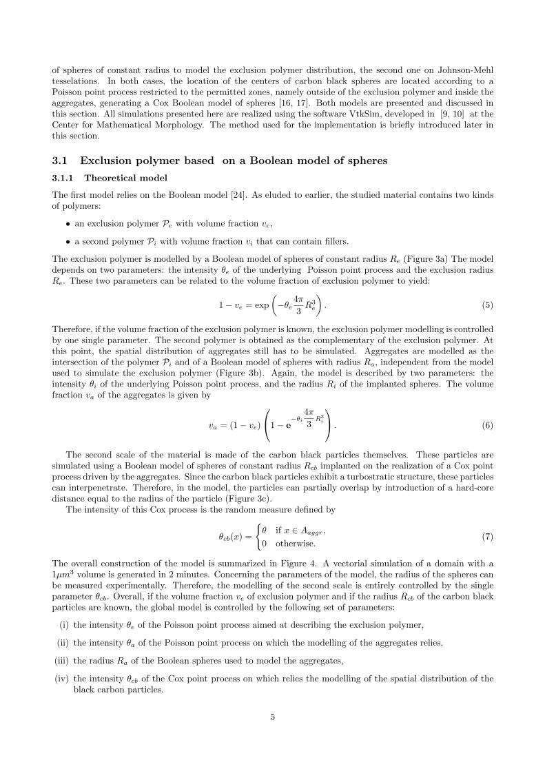
(a) (b) (c)

Figure 7: The three steps of the construction of the model: (a) exclusion polymer (Johnson-Mehl mosaic);(b) aggregates; (c) carbon black particles network (ve = 0.2; θe = 4.10−7 nm−3; Ra = 60 nm; Rcb = 20 nm;simulated volume: (500 nm)3).

paper of [29] provides a unified exposition of random Johnson-Mehl tessellations

The Johnson-Mehl tessellation model was introduced by Johnson and Mehl, mainly to describe crystalliza-tion processes in metallography. Their model can be seen as a variation of the Voronoı model. A Voronoıtessellation is a tessellation built from a Poisson point process P in the space R3. Every point x of R3 isassociated to the class Ci containing all points of R3 closer from the point xi of P than from any other pointof P. Johnson-Mehl tesselations can be seen as a sequential version of the Voronoı model, where the Poissonpoints are implanted sequentially with time. All classes grow then isotropically with the same rate, and thegrowth of crystal boundaries is stopped when they meet. All Poisson points falling in an existing crystal areremoved.

From a mathematical viewpoint, a Johnson-Mehl tessellation is constructed from a sequential Poisson pointprocess where the points xi, i = 1, .., N are implanted sequentially at a time ti, i = 1, .., N . The classesCi, i = 1, .., N corresponding to the points xi, i = 1, .., N are defined by

Ci =

y ∈ R3,∀j 6= i, ti +

‖xi − y‖v

≤ tj +‖xj − y‖

v

. (9)

3.2.2 Exclusion model

In our multiscale model, we rely now on a Johnson-Mehl tesselation to describe the exclusion polymer andits complementary: each class Ci is attributed to the exclusion polymer with the probability ve (= 0.2 in thepresent case) and to the other polymer with the probability 1 − ve, generating a binary Johnson-Mehl mosaic(Figure 7a), that allows us to preserve the symmetry between the geometry of the exclusion polymer and itscomplementary. Here, the two previous parameters of exclusion zone model (Re and θe) are replaced by asingle one, namely the intensity θe of the Poisson point process associated to the Johnson-Mehl tesselation. Theremaining parts of the model are the same as previously. Simulation parameters are the intensity of the Poissonpoint processes attached to each polymer.

A realization of the Johnson-Mehl based model is displayed in Figure 7, as an illustrative example. Avectorial simulation of a domain with a 1µm3 volume is generated in 10 minutes.

The overall construction of the model is summarized in Figure 8. If the volume fraction ve of exclusionpolymer and the radius Rcb of the carbon black particles are known, the global model is controlled by thefollowing set of parameters:

(i) the intensity θe of the Poisson point process associated to the Johnson-Mehl tesselation

(ii) the intensity θa of the Poisson point process on which relies the modelling of the aggregates,

(iii) the radius Ra of the boolean spheres used to model the aggregates,

9

Figure 8: Scheme of the multiscale random model (exclusion polymer made of a Johnson-Mehl mosaic).

ve θe (nm=3) θa (nm−3) Ra (nm) θcb (nm−3) Rcb (nm)0.2 4.0× 10−7 4.0× 10−7 60 3.5× 10−5 18

Table 2: Optimized parameters for the Johnson-Mehl model of exclusion polymer.

(iv) the intensity θcb of the Cox point process on which relies the modelling of the spatial distribution of theblack carbon particles.

Finally, the bound rubber is obtained as before by considering the Boolean difference of a Boolean model ofsphere of constant radius Rcb + t implanted on the centers of the black carbon particles and of the Booleanspheres describing the black carbon particles.

3.2.3 Model fitting from experimental data

As previously, the parameters of the Johnson-Mehl exclusion model are estimated to match the morphologicaldescriptors obtained on the experimental TEM images. The values of the parameters obtained after optimizationare given in the Table 2. The experimental covariance and granulometry are compared with the correspondingcurves obtained by the simulations with fitted parameters on Figure 9. It turns out that the agreement betweenexperimental data and measurements made on simulations is better than in the previous version of the model.A simulated image is shown in Figure 10 and compared to a TEM image.

3.3 Implementation of the models

Simulations of random structures are generally performed on a grid of points (i.e. 2D or 3D images), usingprimary grains based on combination of pixels. The implementation in the software VtkSim relies on a com-pletely different approach based upon level sets and implicit functions. In this approach, primary grains aredescribed by implicit functions [10, 9], which are real valued functions defined in the 3D space. The level sets ofan implicit function Φ are described by an equation of the form Φ(x, y, z) = c, for some constant c. A surfaceis described as a level set of the function Φ, most commonly the set of points for which Φ(x, y, z) = 0. Inthis case, the points for which Φ(x, y, z) < 0 correspond to the interior of the primary grain associated to theimplicit function, the points for which Φ(x, y, z) > 0 to its complementary and the level set Φ(x, y, z) = 0 tothe boundary of the primary grain. Any primary grain can be implemented, whatever its shape, as long as itcan be represented using an implicit function.

In the implicit function approach, complete simulations are generated, using Boolean combinations of pri-mary implicit functions: the union and the intersection of two objects A1 and A2 are defined to yield the

10

(a) (b)

Figure 9: Covariance (a) and granulometry (b) of the simulated material (Johnson-Mehl mosaic for the exclusionpolymer). The simulated curves are represented by the discontinuous lines, the experimental curves by thecontinuous lines.

(a) (b)

Figure 10: Comparison between an experimental (a) and a simulated TEM image (b) for the Johnson-Mehlmosaic model of exclusion polymer.

11

minimum and the maximum, respectively, of their corresponding implicit functions. Thus, we have

Φ(A1 ∪A2) = minΦ(A1),Φ(A2) (10)

andΦ(A1 ∩A2) = maxΦ(A1),Φ(A2). (11)

Similarly, the complementary Ac of set A is defined to be the opposite function

Φ(Ac) = −Φ(A). (12)

Several classical random models can be generated using this method, including among others soft-coreor hard-core Boolean models of spheres. Interestingly, since a combination of implicit functions is itself animplicit function, the realization of a first random simulation enables us to generate multiscale simulations.An interesting feature of the software is that it allows to directly export the simulated microstructures as amesh for further use, like finite elements based computations. Overall, using implicit functions to perform thesimulation allows us to build complex combinations of simulations that we could not process with a pixel basedmethod. Furthermore, vectorial simulations do not require a large amount of computer resources, which allowsus to obtain fast generations of microstructures with very large sizes and numbers of primary grains.

4 Percolation of the carbon black network

It is known that there is a large impact of the connectivity of elements in a random system on its macroscopicbehavior. Controlling the percolation of a network is of major interest in the optimization of the microstructure.In this section, we focus on the percolation of the clusters constituted by the filler particles. Percolating networksof filler can indeed significantly change the mechanical properties of the material. It is therefore of interest tobe able to select simulation parameters that will (or not) create percolating paths in the material.

4.1 General approach

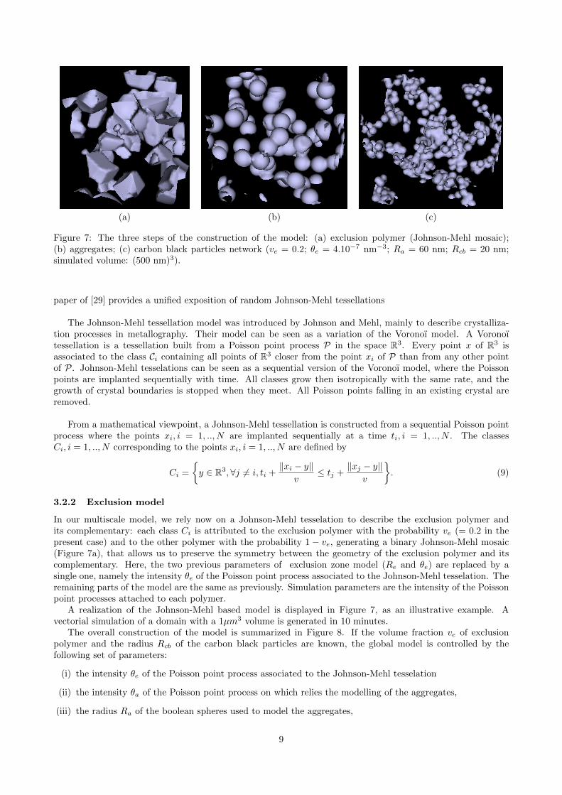
A simulation is said to percolate when a continuous path can be drawn in the filler phase that connects twoopposite faces of the simulation window (a cube in the 3D space). Our aim is to determine the probabilityp that a simulation in a cubic window of length L percolates. To estimate p, N simulations of the randommodel are performed, and the number of simulations that percolate is recorded. A set of parameters leads to apercolating medium when more than 50 percents of the simulations percolate. In this approach, p is estimatedby

pN =1

N

N∑n=1

Pk, (13)

where Pk is the random variable equal to 1 when the simulation percolates and 0 otherwise. The estimatorpN is without bias. We denote by σ2 = p(1 − p) the variance of the random variables Pi, i = 0, .., N. Thevariance of pN is then given by

Var(pN ) =σ2

N. (14)

Hence, Var(pN ) → 0 when N → +∞ and the estimator p converges. For N large enough, according to theCentral Limit Theorem, we have

pN ∼ N (p, σ2/N), (15)

where N (p, σ2/N) denotes the normally distributed law with mean p and standard deviation σ/√N . Therefore,

it can be show that, for N = 100, with confidence 95%,

p− 1.96

√p(1− p)N

≤ p ≤ p+ 1.96

√p(1− p)N

. (16)

Since the quantity p(1− p) is maximal for p = 1/2, yielding p(1− p) = 1/4, we have, in the worst case,

p− 0.098 ≤ p ≤ p+ 0.098. (17)

In mathematical terms, we have

Pp− 0.098 ≤ p ≤ p+ 0.098

≥ 0.95. (18)

This result provides an estimation of the precision of the results obtained in the percolation study.

12

4.2 Percolation algorithm

The aim of the percolation algorithm is to label the connected clusters of filler particles. For each connectedcluster, it is then determined if it is percolating. The percolation algorithm proceeds as follows:

(i) A realization of the model is simulated in a volume of fixed size. At the end of the simulation, the algorithmreturns a list of the coordinates of the filler particles centers.

(ii) Following the approach of [30], the volume is subdivided into cubes of size R, R being the radius of thefiller particle. The coordinates of the filler particles centers are then sorted according to the subvolumes.

(iii) The classical two-pass algorithm is used to label all clusters of filler particles. For a given particle, thenumber of test of intersection is restricted to the adjacent cubes, thus yielding a fast method of construction.

(iv) For each labelled cluster, the algorithm checks if the cluster is percolating.

4.3 Results

The effect of various morphological parameters on the proportion of percolating simulations, estimated on 100realizations for each set of parameters, was investigated for the two previous models of multiscale randommicrostructures: volume fraction of filler, size of aggregates, size of the exclusion polymer clusters. Two sizesof simulations were used, namely (400 nm)3 and (800 nm)3. We report here results obtained on the largestsimulations.

Volume fraction of fillers The volume fraction of fillers is controlled in the simulations by means of theintensity θcb for the centers of the carbon black spheres. The remaining parameters of the simulations are asfollows: ve = 0.2; Re = 30 nm (Boolean model for the exclusion polymer), θe = 4.0× 10−7nm−3 (Johson-Mehlmosaic); va = 0.47; Ra = 60 nm; Rcb = 18 nm; simulated volume: (800 nm)3. The effect of θcb is illustrated byFigures 11a and 11b. From these results, it turns out that the percolation threshold pc (i.e. the lowest value ofp for which more than 50% of realizations percolate) is given by vcb = 0.15 for the Boolean model of exclusionand by vcb = 0.16 for the Johnson-Mehl mosaic. Therefore, the second model shows a slightly higher percolationthreshold. Since the nominal carbon black volume fraction of the real material is vcb = 0.14, it is expected thatits filler network does not percolate, which prevent the material to show a rigid macroscopic behavior.

Aggregates size The effect of the size Raggr of the filler aggregates of the material was studied, while keepingconstant the volume fraction of aggregates. We remind that the volume fraction of aggregates is given by

va = (1− ve)

1− e−θi

4π

3R3

i

. (19)

By properly varying the intensity θaggr, the volume fraction of aggregates remains constant. The simulation pa-rameters are ve = 0.2, Re = 30 nm (Boolean model), , θe = 4.0× 10−7nm−3 (Johnson-Mehl mosaic); va = 0.47;θcb = 3.5× 10−5 nm−3, vcb = 0.14 and Rcb = 18 nm.

The results are displayed in Figures 11c and 11d. Interestingly, we note that, all things otherwise equal,increasing the size of the aggregates results in a monotonous increase of the percentages of simulations thatpercolate. For instance the percentage of percolating simulations climbs from 40 percents when Raggr = 55 nmto 60 percents when Raggr = 70 nm for the two types of models, so that percolation in enhanced for largeraggregates.

Exclusion polymer clusters size From simulations generated by variations of the intensity θe of the Poissonpoint process, the number of exclusion polymer clusters increases (and thus their size is reduced since the volumefraction of exclusion polymer is kept constant). This results in a very slight decrease of the number of percolatingsimulations for both models. Overall, the effect of the exclusion polymer clusters size on percolation propertiesremains rather small.

13

(a) (b)

(c) (d)

Figure 11: (a,b): Influence of the density θcb of filler (with Ve and Va fixed) on the proportion of percolatingsimulations for the two models of exclusion zones: (a) Boolean model of spheres; (b) Johnson-Mehl mosaic.Simulated volume: (800 nm)3. (c,d): Influence of the aggregates size (with Ve, Va and vcb fixed) on theproportion of percolating simulations for the two models of exclusion zones: (c) Boolean model of spheres; (d)Johnson-Mehl mosaic. Simulated volume: (800 nm)3.

14

5 Prediction of viscoelastic properties of simulated 3D microstruc-tures by Fast Fourier Transform (FFT)

In this section a preliminary study of the viscoelastic behavior of the models of random microstructure ispresented. For simplicity, the approach is restricted to the case of two-components media, namely a viscoelasticmatrix and an elastic filler. In the present, accordingly, the mechanical behavior of the various polymers(exclusion polymer, polymer containing the filler, thin layer around carbon-black particles) is supposed to bethe same. In addition, only small deformations of the polymer are considered.

Using a Fourier decomposition in time, strain and stresses are specified as a series of harmonics. This iscommonly accounted for by the introduction of complex elastic moduli. A Fourier decomposition in spaceis introduced, making use of FFT methods to compute the elastic response of highly-contrasted composites.This method is first validated using analytical results for periodic media and compared with explicit time-discretization. It is efficiently applied to arbitrarily complex microstructures provided by a regular grid ofvoxels, such as images of real or of simulated microstructures, and does not require any further meshing ofimages. Extended to the viscoelastic case, it provides full-field reconstructions in time-space, from which theeffective viscoelastic properties of a composite medium are estimated.

In what follows, a complex FFT scheme for viscoelastic composites is introduced and applied to 3D simula-tions of the two previously introduced versions of the multiscale model.This section presents a complex Fourier(FFT) scheme for computing the viscoelastic response of composites. Linear strain-stress relations with elasticand viscoelastic phases are considered. The problem to solve is presented in Section (5.1). The FFT methodused to solve the problem is described in Section (5.2). It is validated in Section (5.3) and used to predict theproperties of rubber containing fillers in Section (5.4).

5.1 Problem setup

Consider a domain V representing a heterogeneous material subject to steady-state oscillatory conditions. Inthe harmonic regime, the time-dependence of the strain ε and stress fields σ at point x is given by the complexfields:

ε(x; t) = ε(x) eiωt, σ(x; t) = σ(x) eiωt, (20)

where the amplitudes ε and σ are second-rank tensor fields, and ω is the frequency applied to the system. Inthe above, ε(x) and σ(x) are complex and do not depend on the time t. The physical strain and stress fieldsare the real parts of ε and σ:

ε(x; t) = R [ε(x; t)] , σ(x; t) = R [σ(x; t)] . (21)

For simplicity, it is assumed that the material contains elastic inclusions (phase α = 2) embedded in a viscoelasticmatrix (phase α = 1). Referring to C2 as the inclusions’s isotropic elastic stiffness tensor, we have, in phase 2:

σ(x; t) = C2 : ε(x; t), σ(x) = C2 : ε(x), (22)

or equivalently,σkk(x) = 3κ2εkk(x), σ′(x) = 2µ2ε

′(x). (23)

where µ2 is the inclusion’s shear modulus, κ2 its bulk modulus, and where the strain and stress deviatoric partsare defined as:

ε′ij = εij − (εkk/3)δij , σ′ij = σij − (σkk/3)δij , (24)

δ being the Kronecker symbol. Inclusions are embedded in a viscoelastic matrix, where the local strain-stressrelation is written generally as:

σ(x; t) =

∫ t

−∞dτ C1(t− τ) :

dε(x; τ)

dτ. (25)

In the above, C1(t) designates a time-dependant fourth-order isotropic tensor with shear and bulk (strain-rate)moduli µ1(t) and κ1(t). Following [5] the time-dependence is removed using Eq. (20):

σkk(x) = 3κ∗1(iω)εkk(x), σ′(x) = 2µ∗1(iω)ε′(x), (26)

15

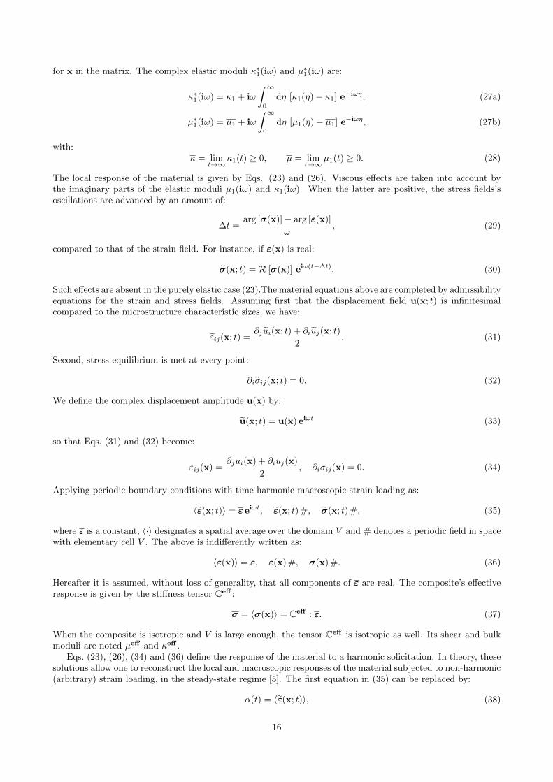
for x in the matrix. The complex elastic moduli κ∗1(iω) and µ∗1(iω) are:

κ∗1(iω) = κ1 + iω

∫ ∞0

dη [κ1(η)− κ1] e−iωη, (27a)

µ∗1(iω) = µ1 + iω

∫ ∞0

dη [µ1(η)− µ1] e−iωη, (27b)

with:κ = lim

t→∞κ1(t) ≥ 0, µ = lim

t→∞µ1(t) ≥ 0. (28)

The local response of the material is given by Eqs. (23) and (26). Viscous effects are taken into account bythe imaginary parts of the elastic moduli µ1(iω) and κ1(iω). When the latter are positive, the stress fields’soscillations are advanced by an amount of:

∆t =arg [σ(x)]− arg [ε(x)]

ω, (29)

compared to that of the strain field. For instance, if ε(x) is real:

σ(x; t) = R [σ(x)] eiω(t−∆t). (30)

Such effects are absent in the purely elastic case (23).The material equations above are completed by admissibilityequations for the strain and stress fields. Assuming first that the displacement field u(x; t) is infinitesimalcompared to the microstructure characteristic sizes, we have:

εij(x; t) =∂j ui(x; t) + ∂iuj(x; t)

2. (31)

Second, stress equilibrium is met at every point:

∂iσij(x; t) = 0. (32)

We define the complex displacement amplitude u(x) by:

u(x; t) = u(x) eiωt (33)

so that Eqs. (31) and (32) become:

εij(x) =∂jui(x) + ∂iuj(x)

2, ∂iσij(x) = 0. (34)

Applying periodic boundary conditions with time-harmonic macroscopic strain loading as:

〈ε(x; t)〉 = ε eiωt, ε(x; t) #, σ(x; t) #, (35)

where ε is a constant, 〈·〉 designates a spatial average over the domain V and # denotes a periodic field in spacewith elementary cell V . The above is indifferently written as:

〈ε(x)〉 = ε, ε(x) #, σ(x) #. (36)

Hereafter it is assumed, without loss of generality, that all components of ε are real. The composite’s effectiveresponse is given by the stiffness tensor Ceff :

σ = 〈σ(x)〉 = Ceff : ε. (37)

When the composite is isotropic and V is large enough, the tensor Ceff is isotropic as well. Its shear and bulkmoduli are noted µeff and κeff .

Eqs. (23), (26), (34) and (36) define the response of the material to a harmonic solicitation. In theory, thesesolutions allow one to reconstruct the local and macroscopic responses of the material subjected to non-harmonic(arbitrary) strain loading, in the steady-state regime [5]. The first equation in (35) can be replaced by:

α(t) = 〈ε(x; t)〉, (38)

16

so that a time-varying macroscopic strain loading α(t) is applied. Taking the Fourier transform of the latter:

α(t) =1

2π

∫ ∞−∞

dω α(ω) eiωt. (39)

The strain field acting in the material is the superposition of the following harmonic responses:

ε(x; t) =1

2π

∫ ∞−∞

dω εω(x) eiωt, (40)

where εω(x) is the complex field solution of Eqs. (23), (26), (34) and (36) with ε = α(ω).

5.2 FFT methods

The purpose of this section is to solve numerically Eqs. (23), (26), (34) and (36) on a grid of voxels, using“Fourier methods” as developed by [31, 8, 26]. The “direct scheme” [31] and “augmented Lagrangian” [26]Fourier methods apply to linear elasticity. The “accelerated scheme” [8], originally given in the context ofconductivity, has been extended to linear elasticity by [26] . We remark that the problem (23), (26), (34)and (36) is mathematically identical to that of linear elasticity, except that complex instead of real fields areconcerned. Thus, FFT methods apply to the viscoelastic problem considered here, as will be seen later. This istrue of other more recent FFT methods like the “rotated” [39] and “variational FFT” [4] schemes. Accordingly,any of these schemes can be implemented for this purpose.

Hereafter, the “discrete scheme” proposed by [41], coupled with the algorithm of [31], is used. A similarscheme has already been investigated in the context of conductivity by [40] leading to much improved convergenceproperties, especially for highly-contrasted composites. The scheme gives for the kth-iteration:

εk+1(q) = ε−G0(q) :[σ(q)− C0 : εk(q)

], (41)

where q is the Fourier wave vector, C0 is a reference elastic tensor and G0(q) its associated Green operator,discretized using a forward and backward finite difference scheme on the rotated grid. The stress field iscomputed at each step in the direct space using the material’s constitutive law, and the strain field is initializedby εk=0 ≡ ε. Convergence strongly depends on C0, an arbitrary (complex) reference tensor, which has to beoptimized. An absolute convergence criterion is defined on stress equilibrium as:

maxx|divσ(x)| ≤ η (42)

where η is the required precision. Care is needed when choosing C0. To ensure that the physical strain andstress fields are symmetric, i.e.:

εkl(x; t) = εlk(x; t), σkl(x; t) = εlk(x; t), (43)

it is necessary to enforce:εkl(x) = εlk(x), σkl(x) = σlk(x). (44)

Hence, the tensors ε and σ are not symmetric in the complex sense. To enforce this, the Green tensor mustsatisfy:

G0ij,kl(q) = G0

ji,kl(q) = G0ij,lk(q) =

[G0kl,ij(q)

]∗. (45)

In turn, this implies:C0ij,kl = C0

ji,kl = C0ij,lk =

(C0kl,ij

)∗= C0

kl,ij , (46)

so that C0 must be real. This is in contrast with optics where we are free to choose complex references (see [2]).In the rest of this work, we choose κ0 = 0.51 [Re(κ∗1) + Re(κ∗2)], µ0 = 0.51 [Re(µ∗1) + Re(µ∗2)], for the bulk andshear moduli of the reference tensor, respectively, where µ∗1,2, κ∗1,2 are the complex elastic moduli in phases 1and 2.

17

0 0.1 0.2 0.3 0.4 0.5spheres volume fraction

1

2

3

Im(µs,p

)

Im(µs) (Cohen)

Im(µp) (Cohen)

Im(µs) (FFT)

Im(µp) (FFT)

0 0.1 0.2 0.3 0.4 0.5spheres volume fraction

0

0.005

0.01

0.015

1-Im(µs,p

)/Re(µs,p

)

Im(µs) (Cohen)

Im(µp) (Cohen)

Im(µs) (FFT)

Im(µp) (FFT)

(a) (b)

Figure 12: Comparison between analytical estimates given by [6] (solid and dashed lines) and FFT results(symbols) for the effective elastic response of a periodic array of spheres with varying volume fraction: imaginarypart of the effective shear moduli µp,s (a) and ratio Im(µp,s)/Re(µp,s).

5.3 Validation and comparison with an explicit time-discretized FFT scheme

In this section, a periodic array of spheres with cubic symmetry is considered. The spheres are purely elasticwith shear and bulk moduli µ2 = κ2 = 1000 GPa, and, for simplicity, the embeding medium is supposed to beMaxwellian. Outside the spheres, the stress σ(t) and strain fields ε(t) satisfy:

σ′(t)dt

t1+ dσ′(t) = 2µ0dε′(t),

σkk(t)dt

t1+ dσkk(t) = 3κ0dεkk(t) (47)

with µ0 = κ0 = 1 GPa, t1 = 1 s. This is equivalent to [5]:

σ′(t) =

∫ t

−∞dτ 2µ1(t− τ)

dε′(τ)

dτ, σkk(t) =

∫ t

−∞dτ 3κ1(t− τ)

dεkk(τ)

dτ, (48)

with:

µ1(t) = µ0e−t/t1H(t), κ1(t) = κ0e

−t/t1H(t), H(t) =

0 if t < 0,1 if t > 0.

(49)

In the above, H(t) is the Heaviside step function. Using (25) the complex elastic moduli in the embeddingmedium read, as functions of the angular frequency ω:

µ∗1(iω) =µ0

1 + 1/(iωt1), κ∗1(iω) =

κ0

1 + 1/(iωt1). (50)

Heareafter the frequency is set to ω = 1[rad/s]. A sphere is discretized in a cubic domain of size 64× 64× 64voxels. The FFT method described in Sec. (5.2) is then used to solve the viscoelastic problem in the complexdomain. The spheres composite has a macroscopic response with cubic symmetry of bulk moduli κs and shearmoduli µp, µs:

C =

κs + 4

3µp κs − 23µp κs − 2

3µp 0 0 0κs + 4

3µp κs − 23µp 0 0 0

κs + 43µp 0 0 0

µs 0 0sym µs 0

µs

(51)

in Voigt notation where ε = (εxx, εyy, εzz, 2εyz, 2εxz, 2εxy) and σ = (σxx, σyy, σzz, σyz, σxz, σxy). FFT Resultsare compared to the analytical estimates in [6] (Figure 12). Excellent agreement between the FFT results andanalytical estimates is found for the complex shear moduli µp,s when the volume fraction of spheres is less than

18

0 5 10 15 t (s)-2

-1

0

1

2

σ12

, ε12

ε12

(time- explicit)σ

12 (time-

explicit)

σ12

(complex scheme)

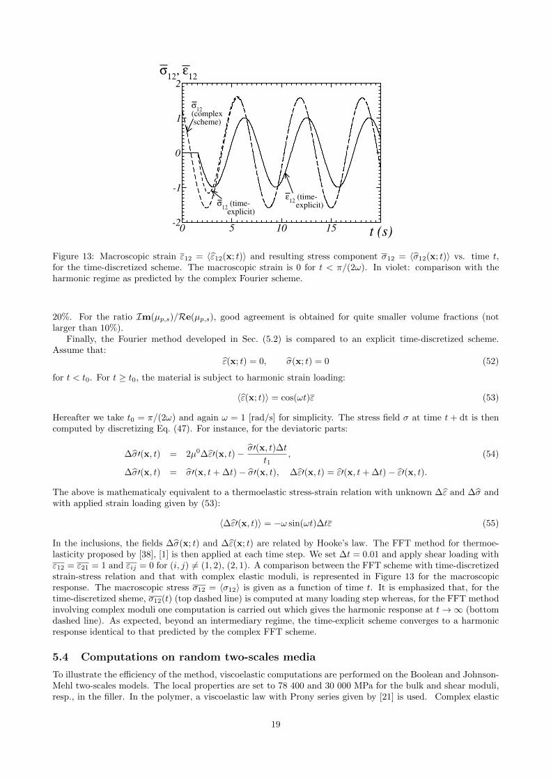
Figure 13: Macroscopic strain ε12 = 〈ε12(x; t)〉 and resulting stress component σ12 = 〈σ12(x; t)〉 vs. time t,for the time-discretized scheme. The macroscopic strain is 0 for t < π/(2ω). In violet: comparison with theharmonic regime as predicted by the complex Fourier scheme.

20%. For the ratio Im(µp,s)/Re(µp,s), good agreement is obtained for quite smaller volume fractions (notlarger than 10%).

Finally, the Fourier method developed in Sec. (5.2) is compared to an explicit time-discretized scheme.Assume that:

ε(x; t) = 0, σ(x; t) = 0 (52)

for t < t0. For t ≥ t0, the material is subject to harmonic strain loading:

〈ε(x; t)〉 = cos(ωt)ε (53)

Hereafter we take t0 = π/(2ω) and again ω = 1 [rad/s] for simplicity. The stress field σ at time t + dt is thencomputed by discretizing Eq. (47). For instance, for the deviatoric parts:

∆σ′(x, t) = 2µ0∆ε′(x, t)− σ′(x, t)∆tt1

, (54)

∆σ′(x, t) = σ′(x, t+ ∆t)− σ′(x, t), ∆ε′(x, t) = ε′(x, t+ ∆t)− ε′(x, t).

The above is mathematicaly equivalent to a thermoelastic stress-strain relation with unknown ∆ε and ∆σ andwith applied strain loading given by (53):

〈∆ε′(x, t)〉 = −ω sin(ωt)∆tε (55)

In the inclusions, the fields ∆σ(x; t) and ∆ε(x; t) are related by Hooke’s law. The FFT method for thermoe-lasticity proposed by [38], [1] is then applied at each time step. We set ∆t = 0.01 and apply shear loading withε12 = ε21 = 1 and εij = 0 for (i, j) 6= (1, 2), (2, 1). A comparison between the FFT scheme with time-discretizedstrain-stress relation and that with complex elastic moduli, is represented in Figure 13 for the macroscopicresponse. The macroscopic stress σ12 = 〈σ12〉 is given as a function of time t. It is emphasized that, for thetime-discretized sheme, σ12(t) (top dashed line) is computed at many loading step whereas, for the FFT methodinvolving complex moduli one computation is carried out which gives the harmonic response at t→∞ (bottomdashed line). As expected, beyond an intermediary regime, the time-explicit scheme converges to a harmonicresponse identical to that predicted by the complex FFT scheme.

5.4 Computations on random two-scales media

To illustrate the efficiency of the method, viscoelastic computations are performed on the Boolean and Johnson-Mehl two-scales models. The local properties are set to 78 400 and 30 000 MPa for the bulk and shear moduli,resp., in the filler. In the polymer, a viscoelastic law with Prony series given by [21] is used. Complex elastic

19

(a) (b)

(c) (d)

Figure 14: (a-b): Real and imaginary parts of the mean stress field σm for a hydrostatic strain loading (εm = 1%)at a frequency ω = 117 Hz. The minimal and maximal values are −47 and 140 Gpa (real part (a)) and −1.0and 6.2 GPa (imaginary part (b)). The stress values are thresholded between 8.68 and 8.73 GPa (real part) and1.5 and 1.6 (imaginary part) to highlight the field patterns in the polymer. (c-d): Real and imaginary parts ofthe shear stress field σ12 for a shear strain loading (εxy = 1%) at a frequency ω = 117 Hz. The minimal andmaximal values are −17 and 44 GPa (real part (c)) and −1.2 and 0.7 GPa (imaginary part (d)). The stressvalues are thresholded between 0 and 6 MPa (real part) and 0 and 1 (imaginary part).

20

10-2

10-1

100

101

102

103

104

2000

2500

3000 Boolean

Johnson-Mehl

ω [rad/s]

Re(κ) [MPa]

Hashincoating

Polymer

10-2

10-1

100

101

102

103

104

101

102

Boolean

Johnson-Mehl

ω [rad/s]

Imag(κ) [MPa]

Polymer

Hashincoating

(a) (b)

10-2

10-1

100

101

102

103

104

1

2

3

Boolean

Johnson-Mehl

ω [rad/s]

Re(µ) [MPa]

Hashincoating

polymer

10-2

10-1

100

101

102

103

10410

-3

10-2

10-1

Boolean

Johnson-Mehl

ω [rad/s]

Imag(µ) [MPa]

Polymer

Hashincoating

(c) (d)

Figure 15: Comparison between the Johnson-Mehl and Boolean sphere models for the exclusion polymer andHashin sphere assemblage: frequency dependence of the effective real part (a) and imaginary part (b) of thecomplex bulk modulus. (c): Real part of the complex shear modulus. (d): Imaginary part.

21

moduli are used for 23 frequencies. Each 3D computation required about 3 hours on a 12-cores computer and800 iterations with η = 3.10−5. No time discretization is used. Domains with size (0.8 µm)3 discretized over(400)3 voxels are simulated.

FFT maps of the mean stress field (opposite of pressure) are shown in Figures 14a and 14b, showing a 2Dsection for the exclusion zones modelled by a Boolean model. The material is submitted to a hydrostatic strainloading, the frequency being ω = 117 Hz. Strong internal stresses in the polymer appear in regions surroundedby fillers. Maps of the shear stress component with shear strain loading are shown in Figures 14c and 14d.

The effective moduli are obtained by averaging the fields calculated by FFT, using a standard homogenizationapproach. The relative precision of the estimated moduli is calculated from the variance of the fields at differentscales, as developed in the statistical RVE approach of [20]. At a frequency ω = 117 Hz, the relative precisionfor the real part and the imaginary part of the bulk modulus is equal to 0.2% and to 0.3%. For the the realpart and the imaginary parts of the shear modulus, it is equal to 17% and 3.8% respectively.

The frequency dependence of the effective complex bulk modulus and of the effective shear modulus areillustrated in Figure 15. FFT data for the Boolean and Johnson-Mehl models are compared to the viscoelasticresponse of the Hashin sphere assemblage [12]. The inner spheres and outer layers in the Hashin coating havethe same properties as the fillers and polymer respectively, and the volume fraction are the same as in themodel (about 10.6%). It has been shown that the bulk and shear moduli of isotropic two-phases viscoelasticcomposites are constrained to a region in the complex plane [11, 27] that generalizes the Hashin and Shtrikmanbounds. The Hashin coating has extremal properties for the bulk modulus in the sense that its bulk moduluslies on the frontier of the region. For the material considered here, the contrast of properties in terms of bulkmoduli is moderate (about 25), and so the Hashin coating is very close to that of the Boolean and Johnson-Mehlmodels, as computed using FFT (Figures 15a and 15b). The situation is sensibly different for the real part ofthe shear modulus, which is 3.104 higher in the filler than in the polymer (Figure 15c). The real part of theshear modulus of the Johnson-Mehl model is higher than that of the Boolean model.

We note that the viscoelastic response of the models is much softer than that of the Hashin assemblage withstiff outer coating, which is not represented in figure 15. Our results are also consistent with that obtainedby [14] in the context of elasticity, where elastic moduli close to the Hashin and Shtrikman lower bounds werepredicted.

6 Conclusion

Multiscale morphological models of random 3D microstructures were developed to simulate the distributionof fillers in rubber materials, accounting for the presence of aggregates and of an exclusion polymer. Thesemodels enable us to study the percolation of carbon black filler as a function of its multiscale distribution. Itwas proved that the two models involving a different morphology for the exclusion polymer do not percolate forthe volume fraction of carbon black contained in the material.

The effective viscoelastic moduli are predicted by Fast Fourier Transforms on 3D simulated images of themicrostructure. The simple method proposed in this work predicts the harmonic response of composites witharbitrary microstructures, frequency per frequency and is restricted to linear materials. The effective bulkmodulus and shear modulus are predicted in a large frequency range (about from 10−1 to 104 rad/s).

Further studies will involve a systematic change of the microstructures by means of the parameters of themodel, and its impact on the effective properties, to find optimal microstructures with respect to the macroscopicbehavior.

Acknowledgements F. Willot is indebted to S. Forest for helpful suggestions regarding the FFT-basedcomputations.

References

[1] A. Ambos, F. Willot, D. Jeulin, and H. Trumel. Numerical modeling of the thermal expansion of anenergetic material. International Journal of Solids and Structures, 60-61:125–139, 2015.

[2] D. Azzimonti, F. Willot, and D. Jeulin. Optical properties of deposit models for paints:full-fields FFTcomputations and representative volume element. Journal of Modern Optics, 60(7):519–528, 2013.

22

[3] M. C. Bergstrom, J. S .and Boyce. Constitutive modeling of the large strain time-dependent behavior ofelastomers. Journal of the Mechanics and Physics of Solids, 46(5):931–954, 1998.

[4] S. Brisard and L. Dormieux. FFT-based methods for the mechanics of composites: A general variationalframework. Computational Materials Science, 49(3):663–671, 2010.

[5] R. Christensen. Theory of viscoelasticity: an introduction. Elsevier, New-York, 2012.

[6] I. Cohen. Simple algebraic approximations for the effective elastic moduli of cubic arrays of spheres. Journalof the Mechanics and Physics of Solids, 52(9):2167–2183, 2004.

[7] A. Delarue and D. Jeulin. 3D morphological analysis of composite materials with aggregates of sphericalinclusions. Image Analysis & Stereology, 22:153–161, 2003.

[8] D.J. Eyre and G.W. Milton. A fast numerical scheme for computing the response of composites using gridrefinement. The European Physical Journal Applied Physics, 6(1):41–47, 1999.

[9] M. Faessel. VtkSim software. http://cmm.ensmp.fr/~faessel/vtkSim/demo/, accessed Jan. 21, 2016.

[10] M. Faessel and D. Jeulin. 3D multiscale vectorial simulations of random models. Proc. ICS13, Beijing,19-22 October 2011.

[11] L.V. Gibiansky and G.W. Milton. On the effective viscoelastic moduli of two-phase media. i. rigorousbounds on the complex bulk modulus. Proceedings of the Royal Society of London A: Mathematical,Physical and Engineering Sciences, 440(1908):163–188, 1993.

[12] Z. Hashin. Complex moduli of viscoelastic composites–I. general theory and application to particulatecomposites. International Journal of Solids and Structures, 6(5):539–552, 1970.

[13] A. Jean, D. Jeulin, S. Forest, S. Cantournet, and F. N’Guyen. A multiscale microstructure model of carbonblack distribution in rubber. Journal of Microscopy, 241(3):243–260, 2011.

[14] A. Jean, F. Willot, S. Cantournet, S. Forest, and D. Jeulin. Large scale computations of effective elasticproperties of rubber with carbon black fillers. International Journal for Multiscale Computational Engi-neering, 9(3):271–303, 2011.

[15] D. Jeulin. Modeles morphologiques de structures aleatoires et de changement d’echelle. These d’etat, 1991.

[16] D. Jeulin. Multi scale random models of complex microstructures. In Materials Science Forum 638, 81–86.Trans. Tech. Publ., 2010.

[17] D. Jeulin. Morphology and effective properties of multi-scale random sets: A review. Comptes RendusMecanique, 340(4):219–229, 2012.

[18] D. Jeulin and A. Le Coent. Morphological modeling of random composites. Proceedings of the CMDS8 58Conference, Varna, Bulgaria, 1996.

[19] V. Jha, A. Thomas, Y. Fukahori, and J. Busfield. Micro-structural finite element modelling of the stifnessof filled elastomers: the effect of filler number,shape and position in the rubber matrix. Proceedings of 5thEuropean Conference on Constitutive Models for Rubber, ECCMR 2007, Paris, France, 2007.

[20] T. Kanit, S. Forest, I. Galliet, V. Mounoury, and D. Jeulin. Determination of the size of the representativevolume element for random composites: statistical and numerical approach. International Journal of Solidsand Structures, 40(13):3647–3679, 2003.

[21] L. Laiarinandrasana, A. Jean, D. Jeulin, and S. Forest. Modelling the effects of various contents of fillerson the relaxation rate of elastomers. Materials & Design, 33:75–82, 2012.

[22] K. Levenberg. A method for the solution of certain problems in least squares. Quarterly of AppliedMathematics, 2:164–168, 1944.

[23] G. Matheron. Introduction aux ensembles aleatoires. Ecole des Mines de Paris, Paris, 1969.

[24] G. Matheron. Random sets and integral geometry. Wiley, New York, 1975.

23

[25] F. Meyer. Iterative image transformations for an automatic screening of cervical smears. Journal ofHistochemistry & Cytochemistry, 27(1):128–135, 1979.

[26] J.C. Michel, H. Moulinec, and P. Suquet. A computational scheme for linear and non-linear composites witharbitrary phase contrast. International Journal for Numerical Methods in Engineering, 52(1-2):139–160,2001.

[27] G.W. Milton and J.G. Berryman. On the effective viscoelastic moduli of two–phase media. ii. rigorousbounds on the complex shear modulus in three dimensions. In Proceedings of the Royal Society of LondonA: Mathematical, Physical and Engineering Sciences, 453, 1849–1880, 1997.

[28] J. Møller. Random tessellations in Rd. Advances in Applied Probability, 21(1):37–73, 1989.

[29] J. Møller. Random Johnson-Mehl tessellations. Advances in applied probability, 24(4):814–844, 1992.

[30] M. Moreaud and D. Jeulin. Multi-scale simulation of random spheres aggregates: Application to nanocom-posites. Proceedings of the ECS 9 Conference, Zakopane, Poland, pp. 341–348, 2005.

[31] H. Moulinec and P. Suquet. A fast numerical method for computing the linear and non linear mechanicalproperties of the composites. Comptes rendus de l’Academie des sciences, Serie II, 318(11):1417–1423,1994.

[32] M. Naito, K. Muraoka, K. Azuma, and Y. Tomita. 3D modeling and simulation of micro to macroscopicdeformation behavior of filled rubber. Proceedings of 5th European Conference on Constitutive Models forRubber, ECCMR 2007, Paris, France, 2007.

[33] J. A. Nelder and R. Mead. A simplex method for function minimization. Computer Journal, 7(4):308–313,1965.

[34] L. Savary, D. Jeulin, and A. Thorel. Morphological analysis of carbon-polymer composite materials fromthick sections. Acta Stereologica (Slovenia), 18(3):297–303, 1999.

[35] R. Schneider and W. Weil. Stochastic and integral geometry. Springer, Berlin, 2008.

[36] J. Serra. Image analysis and mathematical morphology. Academic Press, Inc., Orlando, 1982.

[37] D. Stoyan, W. S. Kendall, and J. Mecke. Stochastic geometry and its applications. Akademie-Verlag, Berlin,1995.

[38] V. Vinogradov and G.W. Milton. An accelerated fft algorithm for thermoelastic and non-linear composites.International Journal for Numerical Methods in Engineering, 76(11):1678, 2008.

[39] F. Willot. Fourier-based schemes for computing the mechanical response of composites with accurate localfields. Comptes rendus de l’Academie des Sciences: Mecanique, 343(3):232–245, 2015.

[40] F. Willot, B. Abdallah, and Y.-P. Pellegrini. Fourier-based schemes with modified green operator forcomputing the electrical response of heterogeneous media with accurate local fields. International Journalfor Numerical Methods in Engineering, 98(7):518–533, 2014.

[41] F. Willot and Y.-P. Pellegrini. Fast Fourier transform computations and build-up of plastic deformation in2D, elastic-perfectly plastic, pixelwise-disordered porous media. In D. Jeulin, S. Forest (eds), “ContinuumModels and Discrete Systems CMDS 11”, pp. 443–449, Paris, 2008. Ecole des Mines.

[42] M. Zahle. Random cell complexes and generalised sets. The Annals of Probability, 16(4):1742–1766, 1988.

24