modelling the behaviour ofsoil-cooling tower-interaction · modelling the behaviour of ... the...
TRANSCRIPT

Loughborough UniversityInstitutional Repository
Modelling the behaviour ofsoil-cooling
tower-interaction
This item was submitted to Loughborough University's Institutional Repositoryby the/an author.
Additional Information:
• A Doctoral Thesis. Submitted in partial fulfilment of the requirementsfor the award of Doctor of Philosophy of Loughborough University.
Metadata Record: https://dspace.lboro.ac.uk/2134/16745
Publisher: c© Emad Aly
Rights: This work is made available according to the conditions of the Cre-ative Commons Attribution-NonCommercial-NoDerivatives 4.0 International(CC BY-NC-ND 4.0) licence. Full details of this licence are available at:https://creativecommons.org/licenses/by-nc-nd/4.0/
Please cite the published version.

University library
• ~ Lo'!ghbprough .UmVerSlty
AuthorlFiling Title ....... A.k1. ... } ..... ~ .. : .. \1 .. · .............. ··.· ........................................................................................
~
Class Mark ................................... \ ................................ .
Please note that fines are charged on ALL overdue items.
0403603986
\\\\\1 \\\\\\\\ \\\ \\\\\ \\\ " \\\ \\ \ \ \\\\ \\\\\

Modelling the Behaviour of
Soil-Cooling Tower-Interaction
By
Emad Hassan Aly
Department of Civil and Building Engineering Loughborough University
~ LOl}ghb"orough • UnIversIty
A dissertation thesis submitted in partial fulfilment of the requirements for the award of PhD,
at Loughborough University
March 2007
©Emad Aly (2007)

---_ . . ' .•... ------'
Class \" \._---! ,\cc 1Nl). D~Ol)b~1~q;~
I dedicate this thesis to my wife and children
for their patience and understanding during
the time of this research.

Modelling the Behaviour of Soil-Cooling Tower-Interaction
Acknowledgments
I am deeply grateful to my supervisors Dr. A. El-Hamalawi and Dr. J. El-Rimawi for their
guidance, encouragement, support and valuable suggestions and discussions for this project.
Special thanks to Dr. El-Hamalawi for providing the source code of GeoFEAP.
I am grateful to my Director of Research, Dr. N. Dixon for his support and guidance. I must
thank our Postgraduate Research Administrator, Helen, for all her support she provided.
Many thanks are due to the Department of Civil and Building Engineering, Loughborough
University for funding this project and also for the facilities they kindly offered throughout
this investigation.
I am also indebted to Professors P. Gould (Washington University, USA), S. Fisenko (Heat
and Mass Transfer Institute, Belarus) and T. Hara (Tokuyama College of Technology, Japan)
for their valuable discussion in the early stages of this study.
Typesetting of this thesis has been done in g..1EX 2c using WinEdt and MiKTeX. Thanks to
Dr. C. Scott (Loughborough University, UK) for his guidance relevant to help with :0-1EX2c.
I would like to acknowledge my deepest gratitude to my family and family in law who have
supported me with their love throughout my time in the UK.
I am also indebted to Dr. T. Hassan (Loughborough University, UK), Professor D. Ingham
(Leeds University, UK), Professor N. Hill (Glasgow University, UK), Professor E. Magyari
(Swiss Federal Institute of Technology, Switzerland), Professor M. Guedda (Universit'e de
Picardie Jules Verne, France), Professor A. Mohammed, Professor E. Elgazzy, Professor
N. Eldabe, Dr. E. Elbarbary and Dr. A. Saad (Ain Shams University, Egypt), for their
encouragement. Finally, many thanks are due to Professor M.S. El Naschie (Frankfurt
University, Germany) as his advice enabled ~e to develop my career in Engineering as an
application of Mathematics.

Modelling the Behaviour of Soil-Cooling Tower-Interaction
Abstract
Natural draught cooling towers belong to a category of exceptional civil engineering struc
tures. These towers are an effective and economic choice among all technical solutions for
the prevention of thermal pollution of natural water resources caused by heated cooling wa
ter in various industrial facilities. They are therefore widely used in most electric power
generation units, chemical and petroleum industries and space conditioning processes. The
cooling tower shell is the most important part of the cooling tower, both in technical and
financial terms and also the most sensitive, since its collapse would put all or part of the
cooling tower out of action for a considerable length of time.
In this thesis, the 2D and 3D behaviour of soil-cooling tower-interaction, via the idealisation
of the structure and soil on the resulting parameters, have been investigated, taking into
consideration the effect of temperature changes in the cooling tower on the simultaneous
interaction of the cooling tower and underlying soil. The temperature effect has been con
sidered because it plays an important role in the design of the cooling towers.
The capabilities of the two-dimensional Geotechnical Finite Element Analysis Program (Ge
oFEAP) have been updated in this project and the new version has been referred to as
GeoFEAP2. New modelling capabilities and the ability to model 3D problems, with accom
panying postprocessing features, were introduced, including 3D first order 8-noded hexa
hedrons. In addition, the Drucker-Prager yield criterion was programmed in GeoFEAP2
to model the elasto-plastic behaviour of the soil. A new 4-noded quadrilateral flat shell
element, based on discrete the Kirchhoff's quadrilateral plate bending element, was also
added to the software to model the elastic behaviour of the cooling tower shell. Further
more, this element was modified to accommodate a temperature profile. The new software
(GeoFEAP2) was then validated for soil behaviour and using several standard widely-used
benchmark problems and the results compared well with the analytical and/or numerical
results obtained by other researchers. A 3D finite element model was created, comprising
the cooling tower, columns support, foundation, and elasto-plastic soil behaviour.
11

ABSTRACT
The analyses of soil-cooling tower-interaction in this thesis have indicated the need to model
the soil and structure as a combined problem, rather than by applying loads onto soil as
geotechnical engineers' model, or by assuming the soil comprises springs and model the
cooling tower, as structural engineers' model. The results have shown how unrealistic the
latter two approaches are. In addition, the analysis necessitates the incorporation of thermal
effects when modelling cooling tower problems. Moreover, from a design point of view, it has
been recommended that circular footing with two cross-columns is better than pad footings
and/or one column. Several other conclusions have been made that would improve the
modelling of soil-cooling tower-interaction. Furthermore, the designer needs to ensure that
enough modelling of soil conditions is done and an extensive site investigation is required
to ensure that the variation in soil properties is represented correctly. Finally, the engineer
needs also to ensure that the site tests performed to measure shear strength with depth via
drilling and other methods needs to go deep enough into the ground to ensure that enough
site information is available when designing the cooling tower.
iii

Contents
Contents viii
List of Figures xv
List of Tables xvi
1 Introduction 1
1.1 Overview...... 1
1.2 Aim and objectives 1
1.3 Background to the research 2
1.4 Structure of the thesis .. . 5
2 Significance of Temperature and Areas of Interest for Cooling Tower 7
2.1 Overview... 7
2.2 Introduction. 7
2.3 Cooling tower terminology 8
2.3.1 Types of cooling towers . 8
2.3.2 Main components of cooling towers 9
2.3.3 Industrial applications 12
2.4 Heat transfer . . . 13
2.4.1 Definitions.
2.4.2 Application to cooling towers
2.4.3 Merkel theory . . . . . . . . .
2.5 Design and manufacture of cooling towers
2.6 Literature review of areas of interest for cooling towers
2.7 Conclusion ........................ .
IV
13
14
.15
17
18
21

CONTENTS
3 Numerical Modelling and Governing Equations of Soil
3.1 Overview ....... .
3.2 Finite element method
3.2.1 The importance of FEM
3.2.2 Stages of FEM .....
3.3 Governing equations of a porous medium
3.3.1 Porous media terminology
3.3.2 Porosity..........
3.3.3 Methods of deriving equation of a porous medium
3.3.4
3.3.5
Continuity equation.
Momentum equation
3.3.5.1 Special case .
3.3.5.2 Geotechnical engineering formulation .
3.4 Soil parameters and behaviour .
3.4.1 Elasto-plastic theory . .
3.4.2 Elasto-plastic governing equations.
3.4.2.1 Elastic behaviour . . . . .
3.4.2.2 Elasto-plastic formulation
3.4.3 State variables ..
3.4.4 Plasticity models ..
3.4.5 Choice of the constitutive model .
3.5 Governing finite element equations
3.5.1 Continuity equation. .
3.5.2 Equilibrium equations
3.6 GeoFEAP and GeoFEAP2 . .
3.6.1 Capabilities of GeoFEAP
3.6.2 Limitations of GeoFEAP .
3.6.3 New features programmed into GeoFEAP
3.7 Conclusion..................
4 Validation of the Software for Soil Model
4.1 Overview ........ .
4.2 Elastic behaviour of soil
4.2.1 2D circular flexible footing: 4-noded quadrilateral elements
4.2.2 2D circular flexible footing: 3-noded triangle elements ...
v
23
23
23
24
24
25
25
27
27
28
29
30
31
31
32
33
33
34
34
35
36
37
37
40
42
42
44
45
45
47
47
47
48
50

5
4.2.3 Effect of Young's modulus on the settlement of 2D
axisymmetric circular footing on two horizontal soil layers
4.2.4 Effect of Young's modulus on the settlement of 2D
axisymmetric circular footing on two vertical soil layers
4.2.5 3D soil-structure interaction with a column.
4.2.5.1 Two horizontal soil layers
4.2.5.2 Two vertical soil layers . .
4.2.6 3D soil-structure interaction for one-storey building
4.3 Elasto-plastic behaviour of soil. . .
4.3.1 Introduction to the problem
4.4
4.3.2 Bearing capacity of a strip footing.
4.3.3 Bearing capacity of a circular footing
Conclusion . . . . . . . . .
Implemented Shell Element
5.1
5.2
5.3
5.4
5.5
Overview ...
Introduction .
Types of shell elements
Elastic shell theory . .
5.4.1 Membrane theory .
5.4.2 Bending theory
Membrane elements .
5.5.1 Introduction.
5.5.2 Elasticity constitutive model.
5.5.2.1 Plane stress condition
5.5.2.2 Plane strain condition
5.5.3 Quadrilateral plane stress element .
5.6 Bending elements ..
5.6.1 Introduction.
5.6.2 Bending of flat plates .
5.6.3 Discrete Kirchhoff quadrilateral element (DKQ)
5.7 Flat shell elements .
5.7.1 Introduction.
5.7.2 Development of stiffness matrix
5.7.3 Coordinate transformation ...
vi
CONTENTS
...... 52
56
60
65
73
76
80
80
81
83
84
87
87
87
88
89
89
89
91
91
92
92
92
93
96
96
97
99
103
103
105
106

5.8 Thermal effects
5.9 Conclusion...
6 Validation of the Implemented Shell Element
6.1 Overview ....... .
6.2 Shell under self-weight
6.2.1 Scordelis-Lo shell roof.
6.2.2 Hemicylindrical shell
6.3 Shell under external load . .
6.3.1 Pinched cylindrical shell with rigid end diaphragm.
6.3.2 Pullout of an open-ended cylindrical shell .
6.3.3 Hemispherical shell with an 18° hole
6.4 Conclusion...................
CONTENTS
108
109
111
111
111
111
114
115
115
116
117
118
7 2D and 3D Study of Soil-Cooling Tower-Interaction 120
7.1 Overview... 120
7.2 Introduction. 120
7.3 2D and 3D cooling tower cases. 125
7.3.1 3D structure case . . . . 125
7.3.2 3D applied load excluding temperature effect. 129
7.3.3 2D axisymmetric applied load excluding temperature effect . 130
7.4 3D combined soil-structure interaction 133
7.4.1 Excluding temperature effect. 133
7.4.2 Including temperature effect . 138
7.5 Parametric study of the 3D cooling tower. 141
7.5.1 Effect of soil shear strength (c) . 141
7.5.2 Effect of soil angle of friction (<p) 143
7.6 Conclusion................. 145
8 Effect of Different Designs for Cooling Tower 148
8.1 Overview... 148
8.2. Introduction . 148
8.3 Type of footings . 156
8.3.1 Circular footing. 156
8.3.2 Pad footings . 165
8.4 Type of columns .. 174
vu

8.4.1 One column .
8.4.2 Two columns
8.5 Vertical soil layers. .
8.6 Horizontal soil layers
8.7 Conclusion......
9 Conclusions and Future Work
9.1 Conclusions ......... .
9.2 Recommendations for future work .
9.2.1 Local-global model
9.2.2 Effect of wind . . .
9.2.3 Effect of earthquake
References
Vlll
CONTENTS
174
179
184
187
190
192
192
195
195
197
197
216

List of Figures
2.1 Typical natural draught cooling tower, Didcot, UK (Nuclear Power Plants
Around the World, 2003). .......... 10
2.2 Diagram of a natural draught cooling tower. 10
2.3 Cross section diagram of a natural draught cooling tower. . 11
2.4 Diagram of the various ways in which a water droplet loses heat; radiation,
convection and evaporation. . . . . . . . . . . . . . . . . . . . . . . . . . .. 15
2.5 (a) A cooling tower comes crashing to the ground during high winds at Fer
rybridge 'C' Power Station in 1965. The aftermath of the incident; (b) Three
of the eight cooling towers were completely destroyed (University of Bristol,
2002). ....................................... 19
3.1 Stages of a finite ~lement analysis (updating from Akin (2003)).
3.2 Diagram of (a) Cartesian co-ordinates system, (b) fluid velocity, up, through
the void patches in the x direction, and (c) the components of the averaged
26
seepage velocity u, v and w in the x, y and z directions respectively. 28
3.3 Idealisation of elasto-plastic behaviour. . . . . . . . . . . . . . . . . 33
3.4 Von Mises and Drucker-Prager yield surfaces (Zienkiewicz and Taylor, 2000). 36
3.5 Problem domain r and boundary O. 38
3.6 General GeoFEAP layout. . . . . . . 43
4.1 Geometric and stratigraphic characteristics for problems 4.2.1, 4.2.3 and 4.2.4. 48
4.2 Finite element mesh for problem 4.2.1. . . . . . 49
4.3 Displacement resultant vector for problem 4.2.1. 49
4.4 Settlement contours in the y-direction for problem 4.2.1.
4.5 Finite element mesh for problem 4.2.2. . . . . .
4.6 Displacement resultant vector for problem 4.2.2.
4.7 Settlement contour in the y-direction for problem 4.2.2.
4.8 Finite element mesh for problem 4.2.3. . . . . . . . . .
IX
50
51
51
51
52

LIST OF FIGURES
4.9 Vertical displacement (ft) at node 161 as a function of EhJEh2 and Eh2 /Eh1 . 53
4.10 Vertical displacement (ft) at the interface level, y = 20 ft, when? = 10, 20, h2
30, 40 and 50. . . . . . . . . . . . . . . . . . . . . . . . . . . . . . . . . . .. 54
4.11 Vertical displacement (ft) at the interface level, y = 20 ft, when? = 10, 20, hi
30, 40 and 50. . . . . . . . . . . . . . . . . . . . . . . . . . . . . . . . . . .. 54
4.12 Vertical displacement (ft) at the interface level, y = 20 ft, when? = ? = 10. 55 112 hi
4.13 Vertical displacement (ft) at the interface level, y = 20 ft, when? = ? = 50. 55 112 hi
4.14 Finite element mesh for problem 4.2.4. . . . . . . . . . . . . 56
4.15 Vertical displacement at nodes 161 and 320 [ft] as a function of? 57 VI
4.16 Settlement contour in the y-direction for problem 4.2.4 when? = 1. 58 VI
4.17 Settlement contour in the y-direction for problem 4.2.4 when? = 20. 58 VI
4.18 Settlement contour in the y-direction for problem 4.2.4 when? = 50. . 58 VI
4.19 Settlement contour in the y-direction for problem 4.2.4 when? = 70. . 59 VI
4.20 Settlement contour in the y-direction for problem 4.2.4 when? = 100. 59 VI
4.21 Geometric and stratigraphic characteristics for problem 4.2.5. 61
4.22 Finite element mesh, top view, for problem 4.2.5. 62
4.23 Finite element mesh, side view, for problem 4.2.5. 62
4.24 Settlement contours, top view, at z = 5 m in the z-direction for problem 4.2.5. 63
4.25 Settlement contours, top view in the z-direction, layer hI - layer h2 interface,
i.e. z = 4 m, for problem 4.2.5. .................... .
4.26 Settlement contours, side view in the z-direction, for problem 4.2.5 ..
4.27 Deviatoric stress values at the soil-structure interaction surface, shown in
figure 4.22, before and after applying the load. . . . . . . . . . . . . . . . .
4.28 Finite element mesh, side view, for problem 4.2.5.1. ....... .
4.29 Settlement contours in the z-direction when? = 10 for problem 4.2.5.1. 112
4.30 Settlement contours in the z-direction when? = 20 for problem 4.2.5.1. h2
4.31 Settlement contours in the z-direction when? = 30 for problem 4.2.5.1. h2
4.32 Settlement contours in the z-direction when ~:~ = 40 for problem 4.2.5.1.
4.33 Settlement contours in the z-direction when? = 50 for problem 4.2.5.1. h2
4.34 Settlement contours in the z-direction when? = 10 for problem 4.2.5.1. hi
4.35 Settlement contours in the z-direction when? = 20 for problem 4.2.5.1. hi
4.36 Settlement contours in the z-direction when? = 30 for problem 4.2.5.1. hi
4.37 Settlement contours in the z-direction when ~h2 = 40 for problem 4.2.5.1. hi
4.38 Settlement contours in the z-direction when? = 50 for problem 4.2.5.1. hi
4.39 Vertical displacement [m] at level z = 4 m when ~hl = 10, 20, 30, 40 and 50. h2
x
63
64
64
65
66
66
67
67
68
68
69
69
70
70
71

LIST OF FIGURES
4.40 Vertical displacement [m] at level z = 4 m when? = 10, 20, 30,40 and 50. 71 h1
4.41 Settlement contours in the z-direction when lIh2 = 0.4999 for problem 4.2.5.1. 72
4.42 Finite element mesh, side view, for problem 4.2.5.2. . . . . . . . . . . . .. 73
4.43 Settlement contours in the z-direction for problem 4.2.5.2 when AV2 = 10. 74
4.44 Settlement contours in the z-direction for problem 4.2.5.2 when AV2 = 20. 74
4.45 Settlement contours in the z-direction for problem 4.2.5.2 when AV2 = 30. 75
4.46 Settlement contours in the z-direction for problem 4.2.5.2 when AV2 = 40. 75
4.47 Settlement contours in the z-direction for problem 4.2.5.2 when AV2 = 50. 76
4.48 Settlement contours in the z-direction when 1/V2 = 0.4999 for problem 4.2.5.2. 77
4.49 (a) Geometric and stratigraphic characteristics for the soil-structure interac-
tion problem considered in Section 4.2.6 and (b) top view for this problem.. 78
4.50 Finite element mesh for the soil-structure interaction problem considered in
Section 4.2.6 for (a) top view of the soil, (b) side view ofthe soil (c) top view
of the rigid footings, (d) top view of the roof, and (e) vertical displacement
contours at the roof. ...................... 79
4.51 Geometric and stratigraphic characteristics for problem 4.3. 80
4.52 Finite element mesh for problem 4.3. . . . . . . . . . . . . . 81
4.53 Failure mechanism of a strip footing on a frictionless soil (Prandtl's wedge
problem). ..................................... 82
4.54 Displacement resultant vectors and contours of the horizontal displacement
for problem 4.3.2. . . . . . . . . . . . . . . . . . . . . 82
4.55 Bearing capacity of a strip footing for problem 4.3.2. 82
4.56 Displacement resultant vectors and contours of the horizontal displacement
for problem 4.3.3. . . . . . . . . . . . . . . . . . . . . . 83
4.57 Bearing capacity of a circular footing for problem 4.3.3. 83
5.1 Membrane, bending and coupled stresses in a shell element. . 91
5.2 Four noded quadrilateral plane stress element. . . . . . . . . 94
5.3 Four noded quadrilateral element in natural coordinate system (~, 1]). 94
5.4 Bending of a thin plate (Cook et al., 2002). . 98
5.5 12 DOF quadrilateral bending element. . . . 100
5.6 Geometry of the DKQ element (Batoz and Tahar, 1982). 101
5.7 Combination of quadrilateral plane and DKQ elements. 104
5.8 Coordinate transformation for quadrilateral element. . 107
6.1 Geometry and boundary conditions for Scordelis-Lo's roof. 112
Ai

LIST OF FIGURES
6.2 Resultant displacement for Scordelis-Lo's problem. . . . . . . . . . . . 113
6.3 Displacement contours in the x-direction for Scordelis-Lo's problem. . 113
6.4 Displacement contours in the y-direction for Scordelis-Lo's problem. . 114
6.5 (a) The geometric, stratigraphic characteristics and boundary conditions, and
(b) finite element mesh for problem 6.2.2. . . . . . . . . . . . . . . . . . . .. 115
6.6 (a) Geometry and boundary conditions for the pinched cylindrical shell, and
(b) mesh for one-eighth of the cylinder. . . . . . . . . . . . . . . . . . . . .. 116
6.7 Geometry and boundary conditions for the pullout of an open-ended cylindri-
cal shell. . . . . . . . . . . . . . . . . . . . . . . . . . . . . . . . . . . . . .. 117
6.8 The hemispherical shell (with 18° central hole) subjected to alternating loads,
(a) top view and (b) side view. ..................... 118
7.1 Coordinates, basic definitions and geometry of a surface of revolution. 121
7.2 Geometric and stratigraphic characteristics for the combined cooling tower-
soil case. . . . . . . . . . . . . . . . . . . . . . . . . . . . . . . . . . . . . .. 122
7.3 3D discretisation for the hyperboloidal shell and columns support, (a) isomet-
ric view and (b) elevation view. . . . . . . . . . . . . . . . . . . . . . . .. 126
7.4 Top view for discretisation of the hyperboloidal shell and columns support. 127
7.5 Meridional stress resultant versus height. . . . 128
7.6 Circumferential stress resultant versus height. 128
7.7 Side view of the 3D discretisation for the applied load case. . 129
7.8 Top view for the 3D discretisation of the applied load case (a) finite element
mesh, (b) title of the material types, and (c) geometry and load applied onto
the footing, represented by the vertical arrows. . . . . . . . . . . . . . . . .. 131
7.9 Deviatoric stress for the 3D applied load at the AA-axis, as shown in figure
7.8(c), and z = -405 ft, -410 ft, -615 ft, -820 ft and -1025 ft, respectively. 132
7.10 Mean pressure for the 3D applied load at the AA-axis, as shown in figure
7.8(c), and z = -405 ft, -410 ft, -615 ft, -820 ft and -1025 ft, respectively. 132
7.11 Settlement contours in the y-direction for the 2D axisymmetric applied load. 133
7.12 Comparison of the vertical settlement (ft) for the 2D and 3D axisymmetric
applied load cases at z = (a) -405 ft, (b) -410 ft, (c) -615 ft, (d) -820 ft
and (e) -1025 ft. . . . . . . . . . . . . . . . . . . . . . . . . . . . . . . . .. 134
7.13 Comparison of the deviatoric stress for the 3D applied load and combined SSI
cases at the AA-axis and z = -405 ft, excluding temp·erature effect. . . . .. 135
XlI

LIST OF FIGURES
7.14 Comparison of the deviatoric stress for the 3D applied load and combined SSI
cases at the AA-axis and z = -410 ft, excluding temperature effect. . . . .. 136
7.15 Comparison of the mean pressure for the 3D applied load and combined SSI
cases at the AA-a..xis and z = -405 ft, excluding temperature effect. . . . . . 136
7.16 Comparison of the settlement for the 3D applied load and combined SSI cases
at the AA-axis and z = -405 ft, excluding temperature effect. . . . . . . .. 137
7.17 Comparison of the settlement for the 3D applied load and combined SSI cases
at the AA-axis and z = -410 ft, excluding temperature effect. . . . . . . .. 137
7.18 Comparison of the deviatoric stress for the 3D combined SSI case when T = O°C, 45°C and 70°C at z = -405 ft. . . . . . . . . . . . . . . . . . . . . . .. 139
7.19 Comparison of the deviatoric stress for the 3D combined SSI case when T =
O°C, 45°C and 70°C at z = -410 ft. . . . . . . . . . . . . . . . . . . . . . .. 139
7.20 Comparison of the settlement for the 3D combined SSI case when T = O°C,
45°C and 70°C at z = -405 ft.. . . . . . . . . . . . . . . . . . . . . . . . .. 140
7.21 Comparison of the settlement for the 3D combined SSI case when T = O°C,
45°C and 70°C at z = -410 ft.. . . . . . . . . . . . . . . . . . . . . . . . .. 140
7.22 Comparison of the deviatoric stress for the 3D combined SSI case when T =
O°C, 45°C and 70°C at z = -410 ft, where c = 0.2 kips/ft2. . . . . . . . . .. 141
7.23 Comparison of the deviatoric stress for the 3D combined SSI case when T =
O°C, 45°C and 70°C at z = -410 ft, where c = 2 kips/ft2. . . . . . . . . . .. 142
7.24 Comparison of the deviatoric stress for the 3D combined SSI case when T =
O°C, 45°C and 70°C at z = -410 ft, where c = 13 kips/ft2. . . . . . . . . .. 142
7.25 Comparison of the deviatoric stress for the 3D combined SSI case when T =
O°C, 45°C and 70°C at z = -410 ft, where cp = 0°. . . . . . . . . . . . . . .. 143
7.26 Comparison of the deviatoric stress for the 3D combined SSI case when T =
O°C, 45°C and 70°C at z = -410 ft, where cp = 10°. . . . . . . . . . . . . .. 144
7.27 Comparison of the deviatoric stress for the 3D combined SSI case when T =
O°C, 45°C and 70°C at z = -410 ft, where cp = 20°. . . . . . . . . . . . . .. 144
8.1 Geometric and stratigraphic characteristics for the cooling tower shell, two
columns, pad footings and soil case. . . . . . . . . . . . . . . . . . . . . . .. 150
8.2 3D discretisation for the cooling tower shell, two columns and circular footing
where (a) top view, (b) isometric view and (c) elevation view. ........ 151
8.3 3D discretisation for the cooling tower shell, one column and circular footing
where (a) top view, (b) isometric view and (c) elevation view. ........ 152
xiii

LIST OF FIGURES
8.4 3D discretisation for the cooling tower shell, two columns and pad footings
where (a) top view, (b) isometric view and (c) elevation view. ........ 153
8.5 Typical natural draught cooling tower in Trino Vercellese, Italy (a) design
and construction of two towers, and (b) one column attached to pad footings
(Bierrum, 2005). ................................. 154
8.6 3D discretisation for the cooling tower shell, one column and pad footings
where (a) top view, (b) isometric view and (c) elevation view. ........ 155
8.7 Comparison of the deviatoric stress at z = -405 ft in the case of circular
footing with one column and two columns for (a) T = O°C, (b) T = 45°C and
(c) T = 70°C. . . . . . . . . . . . . . . . . . . . . . . . . . . . . . . . . . .. 158
8.8 Comparison of the deviatoric stress at z = -410 ft in the case of circular
footing with one column and two columns for (a) T = O°C, (b) T = 45°C and
(c) T = 70°C. . . . . . . . . . . . . . . . . . . . . . . . . . . . . . . . . . .. 160
8.9 Comparison of the vertical settlement [ft] at z = -405 ft in the case of circular
footing with one column and two columns for (a) T = O°C, (b) T = 45°C and
(c) T = 70°C. . . . . . . . . . . . . . . . . . . . . . . . . . . . . . . . . . .. 162
8.10 Comparison of the vertical settlement [ft] at z = -410 ft in the case of circular
footing with one column and two columns for (a) T = O°C, (b) T = 45°C and
(c) T = 70°C. . . . . . . . . . . . . . . . . . . . . . . . . . . . . . . . . . .. 164
8.11 Comparison of the deviatoric stress at z = -405 ft in the case of pad footings
with one column and two columns for (a) T = O°C, (b) T = 45°C and (c) T
= 70°C. .. . . . . . . . . . . . . . . . . . . . . . . . . . . . . . . . . . . .. 167
8.12 Comparison of the deviatoric stress at z = -410 ft in the case of pad footings
with one column and two columns for (a) T = O°C, (b) T = 45°C and (c) T
= 70°C ....................................... 169
8.13 Comparison of the vertical settlement [ft] at z = -405 ft in the case of pad
footings with one column and two columns for (a) T = O°C, (b) T = 45°C
and (c) T = 70°C. ................................ 171
8.14 Comparison of the vertical settlement [ft] at z = -410 ft in the case of pad
footings with one column and two columns for (a) T = O°C, (b) T = 45°C
and (c) T = 70°C. ................................ 173
8.15 Comparison of the deviatoric stress at z = -405 ft in the case of one column
attached to circular and pad footings for (a) T = O°C, (b) T = 45°C and (c)
T = 70°C ...................................... 176
XIV

LIST OF FIGURES
8.16 Comparison of the deviatoric stress at z = -410 ft in the case of one column
attached to circular and pad footings for (a) T = O°C, (b) T = 45°C and (c)
T = 70°C ...................................... 178
8.17 Comparison of the deviatoric stress at z = -405 ft in the case of two columns
attached to circular and pad footings for (a) T = O°C, (b) T = 45°C and (c)
T = 70°C ...................................... 181
8.18 Comparison of the deviatoric stress at z = -410 ft in the case of two columns
attached to circular and pad footings for (a) T = O°C, (b) T = 45°C and (c)
T = 70°C ...................................... 183
8.19 Comparison of the deviatoric stress in the case of two columns attached to
circular footing and vertical soil layers at (a) z = -405 ft and (b) z = -410 ft. 185
8.20 Comparison the vertical settlement [ft] in the case of two columns attached to
circular footing and vertical soil layers at (a) z = -405 ft and (b) z = -410 ft. 186
8.21 Comparison of the deviatoric stress for one soil layer and horizontal soil layers
at z = -410 ft in the case of two columns attached to circular footing for (a)
T = O°C, (b) T = 45°C and (c) T = 70°C. . . . . . . . . . . . . . . . . . .. 189
9.1 Local-global FE model of (a) a cooling tower, where L1 = rotational shell
elements, L2 = transitional shell elements, L3 = general shell elements and
L4 = discrete column elements; (b) element discretisation with various ele-
ments (Hara a~d Gould, 2002). ......................... 196
9.2 Adjacent buildings to (a) one cooling tower, (b) group of five cooling tow-
ers, and (c) group of eight cooling towers (Nuclear Power Plants Around the
World, 2003). . . . . . . . . . . . . . . . . . . . . . . . . . . . . . . . . . .. 198
xv

List of Tables
5.1 Summery of plate and shell element development (Mackerle, 2002). ..... 89
7.1 Geometrical details for the hyperbolic cooling tower (Gould, 1985) and soil
used in the analysis. ............................ 123
7.2 Material properties used in the analysis (Gould (1985), Bowles (1988)). 123
7.3 Thickness of the cooling tower shell (Gould, 1985). ........... 127
XVI

Modelling the Behaviour of Soil-Cooling Tower-Interaction
Nomenclature
a Radius at throat level of cooling tower
{ a} Nodal displacement vector
A Area of transfer surface per unit of volume tower
A Integer constant
b Characteristic dimension of the cooling tower shell, defined by
bx, by, bz
[B]
c
{d}
D
[D]
E
[E]
9
gx, gy, gz
gw
g
G
H
i, j, k
[J]
equations (7.2) and (7.3)
The body forces per unit volume in the x, y and z directions, respectively
Strain-displacement matrix
Cohesion of the soil
Displacement inside the element
Flexural rigidity of the plate
Matrix describes the material moduli
Young's modulus
Matrix defined by equation (3.33)
Magnitude of the acceleration due to gravity
Components of the acceleration vector due to gravity in the
x, y and z directions, respectively
water unit weight
The gravitational force per unit mass
Gas mass
Horizontal soil layers
Arbitrary functions, chosen as displacement
Vertical distances from the throat to the base and top of the cooling tower
shell, respectively
Enthalpy
The unit vectors in the x, y and z directions, respectively
Jacobian matrix
XVll

k
k
kl
ks
kt
J{
[K]
[K]
L
[L]
{m}
n
nj
{n}
[N]
p
p
q
Q
rt, rs
Rx, Ry ,
S
t
t
Tand T
T1, T2
1L, V, W
u, v, w
Rz
Heat transfer coefficient
Permeability of the porous media
Parameter defined in equation (3.28)
Slope of ground depth of variation of c.
NOMENCLATURE
Curvature parameter of the cooling tower shell defined by equation (7.5)
Specific permeability of the porous media
Stiffness matrix
Permeability matrix
Water rate
Matrix defined by equation (3.42)
Vector defined by equation (3.38)
Porosity of a porous medium
Directions cosines of the outward normal vector {n}
Outward normal vector
Matrix of the shape functions
Load point (Chapter 6)
Mean pressure defined by equation (3.21)
Deviatoric stress defined by equation (3.22)
Plastic potential function
Top and base radius of cooling tower respectively
Reaction at supports in the x, y and z directions, respectively
Closed curve surrounding the boundary area r of the domain
Time
Thickness of shell
Temperature
Hot and water temperature, respectively
Meridional, circumferential and normal displacement, respectively
Components of the average seepage velocity in the x, y and z
directions, respectively
up, vp, wp Fluid velocity through the void patches in the x, y and z
directions, respectively
XVlll

x, y, z
Greek Symbols
0:
, r .6..x,
6ij
E
e 8
8L
:\
[A]
1/
p
e
.6..y, .6..z
Vertical soil layers
Artificial seepage velocity
Effective tower volume,
NOMENCLATURE
Volume element which consists of both fluid and solid phases,
=.6..x.6..y.6..z
Weight of the structure in the x, y and z directions, respectively
Cartesian co-ordinates
Coefficient of thermal expansion
Parameter defined by equation (3.28)
Rotations of the normal to the un deformed middle surface in the
xz and yz planes respectively
Unit weight of the material
Boundary area of the domain n Mesh sizes in x, y and z directions respectively
Kronecker's function
Strain
Time integration parameter
Circumferential angle from plane of the reference meridian
Lode's angle defined by equation (3.23)
Lame's coefficient defined by equation (3.18)
:rvlatrix for the transformation of coordinates from the global
to the local axis
Dynamic viscosity of the fluid
Lame's coefficient defined by equation (3.18)
Poisson's ratio
Density
The angle between the outward normal to the body surface
and downward vertical direction
XIX

(J"
(J" x, (J"y, (J"z
T
cP
[<I>]
tp
n
Subscripts
0
as
aw
b
f hI, h2
m
pp
v
VI, V2
w
Superscripts
(1)
(2)
* e
p
o
T
Stress
Normal stress in x, y and z directions respectively
Shear stress
Angle of friction
Flux matrix defined by equation (3.43)
NOMENCLATURE
Angle between axis of revolution and normal to the shell's surface
Domain volume of the problem
Initial
Air steam
Saturated air at water temperature
Bending action
Fluid
Horizontal soil layer
Membrane action
Pore pressure
Void space or vertical soil layer
Vertical soil layers
Water
Value of the parameter at time t
Value of the parameter at time t + ~t Value of the parameter at nodes
Virtual of the parameter
Elastic (Chapter 4), Element (Chapter 5)
Plastic
Degree
Transpose of a matrix/vector
xx

CHAPTER 1
Introduction
1.1 Overview
The aim of this chapter is to introduce the structure of this thesis, the research conducted
during this PhD and the background to it.
1.2 Aim and objectives
The aim of this project is to study the soil-structure interaction of cooling towers taking into
consideration the effect of temperature changes in the cooling tower on the simultaneous
interaction of the cooling tower and underlying soil. This will be investigated in 2D and 3D.
The objectives of this research are:
1. Implementing and examining the behaviour of a four noded quadrilateral flat shell
element based on Kirchhoff's assumptions and modifying it to accommodate a tem
perature profile.
2. Extending the capabilities of the two-dimensional Geotechnical Finite Element Analy
sis Program (GeoFEAP) (Espinoza et al., 1995) to model 3D soil-structure interaction
problems, incorporating the modelling of thermal aspects of soil-structure interaction
in both 2D and 3D.
3. Testing and validating this updated GeoFEAP2 software for two and three dimensions
soil-structure interaction and shell element.
1

1.3 Background to the research
4. Investigating the soil-structure interaction using GeoFEAP2 taking into consideration
the temperature changes in the cooling tower.
5. Investigating the effect of the modelling method of soil-structure interaction, via the
idealisation of the structure and soil on the resulting parameters.
1.3 Background to the research
Natural draught cooling towers belong to a. category of exceptional civil engineering struc
tures. These towers are an effective and economic choice among all technical solutions for
the prevention of thermal pollution of natural water resources caused by heated cooling wa
ter in various industrial facilities. They are therefore widely used in most electric power
generation units, chemical and petroleum industries and space conditioning processes. The
shell is the most important part of the cooling tower, both in technical and financial terms
(30% to 45% of the total cost) and also the most sensitive, since its collapse would put all
or part of the cooling tower out of action for a considerable length of time. Hence, the shell
is one of the fundamental factors influencing the life of the cooling tower (Jullien et al., 1994).
In November 1965, three of the eight cooling towers suddenly collapsed under a storm at
the Ferrybridge Power Station in Yorkshire (UK). Details of the collapse were reported ex
tensively in the literature (e.g. CEGB, 1965; Pope, 1994). The collapse was attributed to
insufficient vertical reinforcement to resist the uplift forces, and to wind-induced vibrations
causing vertical cracking on shells (Bosman et al., 1998). In September 1973, a single 137 m
tall cooling tower collapsed under moderate winds at Adeer Nylon "\iVorks power plant just
off the Southwest coast of Scotland. Formal investigations into the collapse (ICI, 1974) con
cluded that meridional curvature imperfections in the shell were responsible for the failure.
A third incident of a cooling-tower collapse in the UK occurred in Lancashire in January
1984, when one tower at Fiddlers Ferry Power Station collapsed in wind gusts exceeding 125
km/h, details of this collapse have been reported extensively in the literature (e.g. CEGB,
1984; Pope, 1994). As a result, much research (Bamu and Zingoni, 2005; Nasir et al., 2002)
into the structural behaviour of hyperbolic axisymmetric shell structures has been carried
out using the finite element method. Some of the areas of major interest include:
• Heat and mass transfer inside the cooling tower (e.g. Hawlader and Liu, 2002; Patel
et al., 2004).
2
1.3 Background to the research
• Structural stability and foundation settlement (e.g. Min, 2004; Noh et al., 2003).
• Non-linear analysis of cooling tower shells (e.g. Lang et al., 2002; Waszczyszyn et al.,
2000).
• Static and pseudo-static effects of wind and earthquake loading (e.g. Baillis et al., 2000;
Orlando, 2001).
• Durability of cooling towers (e.g. Busch et al., 2002; Harte and Kratzig, 2002).
Other important aspects of investigating cooling tower behaviour is temperature and wind
(Kloppers, 2003). However, the contribution of thermal stresses to the total stress distri
bution in cooling tower under combined loading (wind pressure, gravity load etc.) remains
significant (Bosak and Flaga, 1996; Sharma and Boresi, 1980; Sudret et al., 2005). In addi
tion, the total tower height is generally fixed by the thermal design (Busch et al., 2002). In
this thesis, the attention is therefore given to the temperature effect, as this focus provides
greater scope for original contributions. Effect of wind will be considered as future work, as
stated in Section 9.2.
Heat transfer between the hot air inside the cooling tower and ambient air establishes a vari
able temperature field in the wall of the tower. The temperature difference between internal
and external faces of the cooling tower shell causes bending moments in the shell (Ravinder
et al., 1996). In particular, the temperature changes create stresses on the upper concrete
part of the cooling tower, especially near the bottom of the tower. It should be noted that
this thermal gradient causes the concrete to crack vertically along the meridians (Rao and
Ramanjaneyulu, 1993). In addition, these stresses may then change the loading on the foun
dation and soil respectively. The temperature value at the internal face of the cooling tower
is in general in the range of 28°C to 39°C (Kloppers, 2003; Kloppers and Kroger, 2003, 2005;
Wittek and Kditzig, 1996). This is the standard operating temperature range which depends
on the ratio of the water to gas mass flow (L / G) of the cooling tower. It should be noted that
temperature plays an important role in the design of cooling towers (Kim et al., 2001; Ravi
et al., 1996). In particular, a change in the (L/G) pf the cooling tower will change the tower
characteristics (Cheremisinoff and Cheremisinoff, 1989; Kloppers and Kroger, 2005). More
design details are covered in parts 2, 3 and 4 of the British Standard BS4485 (1988a,b, 1996).
In general, two approaches are usually used for studying the soil-structure interaction. In
the first, the reactions of the structure are modelled as loads applied directly to the soil (e.g.
3

1.3 Background to the research
Almeida and Paiva, 2004), neglecting the structure itself. In this case the soil behaviour is
the main area of interest. \Vhen interest in the structural behaviour is more important, the
soil is modelled using flexible springs (Jullien et al., 1994). These are however very approx
imate methods and do not account for the actual interaction between soil and structure.
Less attention was given to the investigation of soil-structure interaction. If, however, the
simultaneous interaction of soil and structure was modelled then more accurate results would
be obtained.
The above indicates that the proper and more accurate way of modelling the soil and struc
ture is to model them simultaneously using both geotechnical and structural approaches in
order to fully understand the soil-structure interaction that occurs for cooling towers. To the
best of the author's knowledge, no complete 3D model including both cooling tower and soil
as one continuous medium has been modelled. Shu and Wend a (1990) modelled a:dsymmet
rical cooling tower-soil, excluding temperature, and concluded that structure-soil interaction
must be considered in order to understand the truly dynamic behaviour of structure and soil.
The effect of temperature, which has generally been ignored in early designs due to lack of
adequate knowledge (Bamu and Zingoni, 2005), has to also be included as it is a major de
sign criterion in cooling towers. The tower considered for this analysis is a column supported
hyperbolic cooling tower with a height of 520 ft (158.5 m), which has dimensions in the range
of the tallest modern cooling towers, earlier analysed by Gould (1985) and later by other re
searchers (e.g. Aksu, 1996; Iyer and Rao, 1990; Karisiddappa et al., 1998) for further studies.
The two-dimensional Geotechnical Finite Element Analysis Program (GeoFEAP) (Espinoza
et al., 1995) is used in this project because it supports geomechanical analysis. The availabil
ity of the basic source code, in addition to being well-tested and used by various researchers
(e.g. Bray, 2001; Pestana et al., 1996) facilitates the validation process. GeoFEAP is there
fore updated in this project and the new version will be referred to as GeoFEAP2. This
software will be used to create a 3D finite element model to comprise the shell element to
represent the cooling tower, columns support, foundation, and elastic and elasto-plastic soil
behaviour.
4
1.4 Structure of the thesis
1.4 Structure of the thesis
This thesis is divided into the following remaining chapters:
• In Chapter 2, cooling towers' terminology and its two types, natural and mechanical
draught, are presented. The main components ofthe natural draught tower, or simply
cooling tower as considered during this research, are introduced. In addition, applica
tion of heat and mass transfer processes and Merkel theory are discussed to show the
importance of temperature when designing these towers. Literature review of areas of
interest for cooling towers is also introduced.
• The aim of Chapter 3 is to present the governing finite element equations for the
soil-structure interaction analysis in two and three dimensions, which have been used
in the present numerical modelling and software (GeoFEAP2). First, the theory of
porous media, as a general ca.'3e for soil, is introduced and then the governing equations
(continuity and momentum) for the fluid flow through a porous medium are presented.
In addition, soil parameters and elasto-plastic behaviour are discussed. Finally, an
appropriate constitutive model, Drucker-Prager, is then chosen to be used in this
study.
• In Chapter 4, validation of the new software (GeoFEAP2) when modelling the soil
structure interaction is investigated for elastic and elasto-plastic soil behaviour. This·
validation is studied for one- and two- horizontal and vertical soil layers in two and
three dimensions with different types of elements and loads.
• The main aim of Chapter 5 is to introduce the four noded quadrilateral flat shell ele
ment which is used in this research to model the cooling tower shell. First, membrane
and bending elements based on Kirchhoff's assumptions are used to develop this ele
ment, then the stiffness matrix for it is presented. Thermal effects upon this flat shell
element are presented.
• In Chapter 6, five standard widely-used 'obstacle course' benchmark shell problems,
under self weight (Scordelis-Lo shell roof and hemicylindrical shell) and external load
(pinched cylindrical shell with rigid end diaphragm, pullout of an open-ended cylin
drical shell and hemispherical shell with an 18° hole), are presented to validate the
4-noded quadrilateral flat shell element which has been introduced in Chapter 5.
These problems have been modelled using the GeoFEAP2 and the results are com
pared with those obtained by other researchers.
5

1.4 Structure of the thesis
• Comparisons between the 2D and 3D applied load, and between 3D applied load and
combined cooling tower-foundation-soil are then investigated and examined in Chap
ter 7. In addition, the behaviour of the soil layer is investigated in the presence of
temperature effect at the shell and a change in the effect of soil shear strength and soil
angle of friction.
• In Chapter 8, the soil behaviour for different types of footings, circular and pad, affected
by different types and configurations of columns are investigated in the presence of the
temperature effect on the cooling tower shell. Vertical and horizontal soil layers are
also considered.
• A summary and conclusions of this research with recommendations for future work are
presented in Chapter 9.
6

CHAPTER 2
Significance of Temperature and
Areas of Interest for Cooling Tower
2.1 Overview
The main objective of this chapter is to discuss the importance of temperature when de
signing cooling towers. It should be noted that thermal loading has generally been ignored
in early designs of cooling towers due to lack of adequate knowledge (Bamu and Zingoni,
2005). Hence, cooling tower terminology, the application of heat transfer theory and litera
ture review of areas of interest for cooling tower are discussed'.
2.2 Introd uction
Heat is discharged in power generation, refrigeration, petrochemical, steel processing and
many other industrial plants. In many cases, this heat is discharged into the atmosphere
with the aid of a cooling tower via a secondary cycle with water as the process fluid. In
particular, when water changes state from liquid to vapour or steam, an input of heat energy
must take place, known as the latent heat of evaporation. Cooling towers take advantage of
this change of state by creating conditions in which hot water evaporates in the presence of
moving air. Hence, cooling towers are a very important part of many chemical plants.
Cooling tower designs are generally based on the ambient air dry-bulb temperature, mea
sured at,· or near the ground with a corresponding dry adiabatic lapse rate. The average
temperature of the air at the inlet of the tower may deviate significantly from the measured
7

2.3 Cooling tower terminology
air temperature near the ground due to temperature inversions. The effective inlet air tem
perature is higher than the measured air temperature at ground level because the tower
draws in air from high above the ground (Kloppers and Kroger, 2005).
The reinforced concrete cooling tower is generally subjected to a dead-weight, temperature
gradient load due to the temperature difference between the inside and outside of the shell
and the effects of creep/shrinkage of concrete (Choi and Noh, 2000). Hence, a better under-
. standing of evaporative cooling of water in cooling towers is necessary both for modernisation
of the existing cooling towers, and for predicting the efficiency of newly designed ones because
the development of new types of cooling towers requires the conduction of many thermal
and hydraulic tests that are too costly (e.g. Dreyer and Erens, 1996; Fisenko et al., 2002).
2.3 Cooling tower terminology
The cooling towers built for industrial purposes are amongst the largest shell structures
constructed in the form of hyperbolic shells of revolution supported by closely spaced inclined
columns. Although the art of evaporative cooling is quite ancient, the first natural draught
cooling tower was only constructed in 1916 at the Emma Pit in the Netherlands by the
Dutch State Mines (Bowman and Benton, 1997). The world's tallest cooling tower is 200 m
high and is situated at the Niederaussem power plant in Germany (Busch et al., 2002; Harte
and Kratzig, 2002).
2.3.1 Types of cooling towers
Although there are many different types of cooling tower, they can be divided into two main
categories; natural draught and mechanical draught towers, depending on the method by
which air is moved through the tower. However, there are four major components which go
into the make-up of a cooling tower (Hill et al., 1990):
1. the packing,
2. drift eliminators,
3. the water distribution system, and
4. the fans (except for natural draught towers).
8

2.3 Cooling tower terminology
The natural draught towers depend upon natural forces to move air through the pack and
they are designed using very large concrete chimneys to introduce air through the media.
These towers are an effective and economic choice among all technical solutions for the pre
vention of thermal pollution of natural water resources caused by heated cooling water in
various industrial facilities (Min, 2004).
The mechanical draught towers utilise large fans to force air through circulated water. One
of the major advantages of the mechanical draught tower, is that it can cool to a lower water
temperature than a natural draught tower.
In this research, more attention is given to the natural draught cooling tower. However,
more details about mechanical cooling towers can be found in Fisenko et al. (2004).
2.3.2 Main components of cooling towers
Figure 2.1 shows a typical natural draught cooling tower (Nuclear Power Plants Around
the World, 2003), while figures 2.2 and 2.3 show the outside view and cross section, with
the main components of it respectively. Three main parts can be seen in figures 2.2 and
2.3; shell, plant heat exchange process and soil. The main components inside the shell are
discussed below:
1. Shell (or Casing): the structure enclosing the heat transfer process, necessary to carry
the other main items as shown in figure 2.2. The temperature on the inner surface of
this shell is in the range of 28°C to 39°C (Kloppers, 2003; Kloppers and Kroger, 2003,
2005; Wittek and Kratzig, 1996).
2. Air inlet: the position at which cool air enters and is normally protected by drip-proof
louvers.
3. Air outlet: the position at which warm air leaves the tower as shown in figure 2.2. It
is normally protected by a suitable grill.
4. Drift eliminators: they prevent water droplets from being carried away from the tower
by the airsteam. However, some water loss occurs and this process is called drift loss.
5. \Varm water inlet: the point at which warm water enters the tower. The warm water
comes from processes like air conditioning, manufacturing and electric power genera
tion.
9

2.3 Cooling tower terminology
Figure 2.1: Typical natural draught cooling tower, Didcot, UK (Nuclear Power Plants
Around the World, 2003).
====>
Figure 2.2: Diagram of a natural draught cooling tower.
10

plant heat exchange·
@drift eliminators
droplet in the spray
zone
droplet in the rain
zone
air outlet
2.3 Cooling tower terminology
® hot water distribution system
Figure 2.3: Cross section diagram of a natural draught cooling tower.
11

2.3 Cooling tower terminology
6. Water distribution system: to spread the water as much as possible over the cross
section of the tower.
7. Packing (or Fill): it consists of a system of baffles which ensure maximum contact
between water droplets and cooling air by maximising surface area and minimising
water film thickness. In addition, they slow the progress of the warm water through
the tower. The pack design is therefore very important.
8. Cold water basin (or Tank): to collect the cold water before returning to the plant
heat exchange process. However, as cooling systems suffer many forms of corrosion
and failure, some treatments are made before returning the cold water to the process
(Herro and Port, 1993).
9. Cold water outlet: the point at which the cooled water leaves the tower and is sent
back to the process.
10. Make-up water source: the point at which water added to the circulating water system
to replace evaporation, leakage and drift loss.
Two zones exist; spray zone and rain zone. The spray zone is located between the hot water
distribution system and the packing, while the rain zone is located between the packing and
the basin. In addition, two interactions occur; soil-structure interaction and fluid-structure
interaction.
Figures 2.2 and 2.3 show the cycle of water in the cooling tower. First, the plant heat
exchange process produces warm water which enters the tower at the inlet hot water (5).
Some of this water goes through drift eliminators (4) and carries away through the tower at
air outlet (3). The remaining water is spread by a hot water distribution system (6) in the
spray zone. The air enters the cooling tower at the air inlet (2) then the hot water from the
spray zone meets the air at packing (7) and then droplet in the rain zone. Hence, the water
is cold in this zone and collected at the cold water basin (8), which is fed by water from the
make-up water source. Finally, this cold water goes through outside the cooling tower to the
process at"outlet cold water (9) and then a new cycle then starts.
2.3.3 Industrial applications
The cold water which goes through outside cooling towers is used for many applications, such
as refrigeration plants, air compressors, engines, chemical and refinery plants and turbine
12

2.4 Heat transfer
condenser cooling. In general, the most common applications of cooling towers are supplying
cooled water for air conditioning, electric power generation and nuclear power stations.
2.4 Heat transfer
The objective of this section is to discuss the fundamental concepts of heat transfer and then
its application to cooling towers.
2.4.1 Definitions
Heat is defined as energy transferred between a system and its surroundings as a result of
temperature differences only (Resnick and Halliday, 1996). The science of heat transfer is
devoted to the study of the processes of heat propagation in solid, liquid and gaseous bod
ies. Such processes, because of their highly diversified physico-mechanical nature, are very
complex and usually proceed as a complete complex of heterogeneous phenomena.
There are three mechanisms by which heat transfer can occur; conduction, convection and
radiation. Conduction is the process of heat transfer by molecular motion, supplemented
in some cases by the flow of free electrons through a body (solid, liquid or gaseous) from a
region of high temperature to a regio!! of low temperature (Kakag and Yener, 1995). Heat
transfer by conduction also takes place across the interface between two bodies that are
in contact when they are at different temperatures. The mechanism of heat conduction
in liquids and gases has been postulated as the transfer of kinetic energy of the molecular
movement. Transfer of thermal energy to a fluid increases its internal energy by increas
ing the kinetic energy of its vibrating molecules, and it is measured by the increase in its
temperature. Thus heat conduction is the transfer of kinetic energy of the more energetic
molecules in the high-temperature region by successive collisions to the molecules in the
low-temperature region. Thermal radiation, or simply radiation, is heat transfer in the
form of electromagnetic waves. All substances, solid bodies as well as liquids and gases emit
radiation as a result of their temperature, and they are also capable of absorbing such energy.
The process of heat transfer develops in a different way depending on the physical properties
of the investigated material. Heat transfer is especially affected by the following proper
ties: thermal conductivity, specific heat, density, thermal diffusivity and viscosity. These
13

2.4 Heat transfer
properties have definite magnitudes for each substance and, in general, are functions of the
temperature, and some are also functions of the pressure.
2.4.2 Application to cooling towers
In the case of cooling towers two fluids are involved; air with moisture content up to sat
uration point and water which enters the tower at high temperature and leaves the tower
cooled. The main source of the heat transferred in cooling towers is the latent heat or
evaporative increment and this heat must be extracted from the water as it flows through
the tower. In the next paragraph, the mechanisms by which the water is cooled are discussed.
Figure 2.4 shows the various ways in which a water droplet loses heat. The droplet is
surrounded by a thin film of air which is saturated and remains almost undistributed by the
passing air steam. The transfer of heat takes place in three ways, as shown in figure 2.4:
a. By radiation from the surface of the droplet; this is a very small proportion of the total
amount of heat flow and is usually neglected.
b. By conduction and convection between water and air; the amount of heat transferred
wiII depend on the temperatures of air and water. It is a significant proportion of the
whole.
c. By evaporation, where T2 < T1; this accounts for the majority of heat transfer and
so the whole process is termed evaporative cooling, about 90% of the heat energy is
transferred via evaporation (Hawlader and Liu, 2002). Evaporation is the key to the
successful operation of cooling tower so more discussion has been presented.
The evaporation that occurs when air and water are in contact is caused by the difference
in pressure of water vapour at the surface of the water and in the air. In the cooling tower,
the water and air streams are generally opposed so that cooled water leaving the bottom of
the pack is in contact with the entering air. Similarly, hot water entering the pack will be in
contact with warm air leaving the pack. Evaporation will take place throughout the pack.
It should be noted that at the top of the pack the fact that the air is nearly saturated is
compensated for by the high water temperature and consequently high vapour temperature.
A better understanding of evaporative cooling of water in cooling towers is necessary both
for modernisation of the existing cooling towers and for predicting the efficiency of newly
14

2.4 Heat transfer
designed ones (Fisenko et al., 2002) because the development of new types of cooling towers
requires the performing several thermal and hydraulic costing tests (Dreyer and Erens, 1996).
A detailed investigation of evaporative process in cooling towers can be found in Fisenko
(1992), Petruchik and Fisenko (1999), Petruchik et al. (2001) and Fisenko et al. (2002) for
natural draught cooling towers (open towers) and recently in Stabat and Marchio (2004) in
indirect cooling towers (closed towers).
1 1 1 1
bulk water at temperature
T.
film
1 1 1 1 air at temperature
T.
Figure 2.4: Diagram of the various ways in which a water droplet loses heat; radiation,
convection and evaporation.
2.4.3 Merkel theory
The most generally accepted theory of the cooling tower heat transfer process is that devel
oped by Merkel (1925). This theory states that the total heat transfer taking place at any
position in the tower is proportional to the difference between the total heat of the air at
that point and the total heat of the air saturated at the same temperature as the water at
the same point. The Merkel equation can be \VTitten as follows:
(2.1)
15

2.4 Heat transfer
where
k~V = tower characteristic (or Merkel number),
k = heat transfer coefficient,
A = area of transfer surface per unit of volume tower,
V = effective tower volume,
L = water rate,
TI = hot water temperature,
T2 = cold water temperature,
Haw = enthalpy of saturated air at water temperature, and
Has = enthalpy of air steam.
The relation between saturated air enthalpy and temperature is not a simple linear function
of temperature so numerical integration is usually required to solve this integral (Dreyer and
Erens, 1996). Hence, the tower characteristic value can be calculated by solving equation
(2.1) with the Chebyshev numerical method (Fox and Parker, 1968),
kA V TI - T2 (1 1 ) -y- = 4 ~hl + ~h2 + ...... .
where
~hl = value of (Haw - Has)
~h2 = value of (Haw - Has)
~h3 = value of (Haw - Has)
~h4 = value of (Haw - Has)
at
at
at
at
T2 + 0.1 (TI - T2)
T2 + 0.4 (TI - T2 )
TI - 0.4 (TI - T2)
TI - 0.1 (TI - T2 )
(2.2)
Thermodynamics dictate also that the heat removed from the water must be equal to the
heat absorbed by the surrounding air. This relation can be written in a simple form as
(Water Heat + Air Heat\n = (\Vater Heat + Air Heat)out
This expression can be written in mathematical form as follows:
L -
G
where
L / G = liquid to gas mass flow ratio,
H2 = enthalpy of air-water mixture at exhaust wet-bulb temperature, and
HI = enthalpy of air-water mixture at inlet wet-bulb temperature.
16
(2.3)

2.5 Design and manufacture of cooling towers
The tower characteristic (kA VI L) varies with the (L I G) ratio, which can be deduced from
equations (2.2) and (2.3). Careful and accurate analysis of cooling towers are needed to
ensure a precise determination of cooling water temperature. The importance of (LIG) in
the design of cooling tower is discussed below.
2.5 Design and manufacture of cooling towers
Cheremisinoff and Cheremisinoff (1989) and Burger (1989) described the principal criteria
on which the design and manufacture of cooling towers is based as:
1. Achieving maximum contact between air and water in the tower by optimising the
design of tower packing and water distribution system.
2. Minimising the loss caused by water spray escaping from the tower; control of spray
loss is very important in eliminating the risk of infectious diseases being transmitted
to people by the warm moist air.
3. Relating the design of the tower to the volume flow rate of the water to be cooled,
ambient air wet bulb temperature, warm water input temperature and cooled water
output temperature.
4. Understanding and controlling the problems arising from the quality of the water such
as corrosion, fouling and grmvth of bacteria.
5. Taking due account of space limitations at the tower's location and controlling the
noise from it.
It is important to notice the following three key points in cooling tower design:
1. A change in wet bulb temperature (due to atmospheric conditions) will not change the
tower characteristic (kA VI L ).
2. A change in the cooling range will not change (kAV I L).
3. Only a change in the (LIG) will change (kAVIL).
The best way to design the cooling tower is to find a proper (LIG) satisfying such sizes of
cooling tower .. The (LIG) is the most important factor in designing the cooling tower and
related to the construction and operating cost of cooling tower (Kim et al., 2001).
17

2.6 Literature review of areas of interest for cooling towers
2.6 Literature review of areas of interest for cooling
towers
To avoid thermal pollution of lakes and rivers, the heat input to the cooling tower should
be removed artificially using a cooling system. Among many solutions, hyperbolic natural
draught cooling towers are considered to be very effective and most economical. Cooling
towers, especially natural draught ones, are therefore widely used in most electric power
generation units, chemical and petroleum industries and space conditioning processes. In
large power stations only natural draught cooling towers are able to recover the large quantity
of water required for the cooling system. Careful and accurate analysis of cooling towers are
desirable to ensure a precise determination of cooling water temperature. However, cooling
tower shell design practice in the late 1950s and early 1960s did not have access to finite
element techniques and depended on less accurate methods (Bosman et al., 1998). The first
approach to the finite element solution ofaxisymmetric shells was presented by Grafton and
Strome (1963). However, in 1965 three of the eight cooling towers at the Ferrybridge 'C'
power station in UK collapsed, as shown in figure 2.5. Much research into the behaviour of
hyperbolic axisymmetric shell structures has since been carried out since the development
of the finite element method. Areas of interest during the last few decades have included:
1. Thermal effects (eg. Fisenko (1992), Mertes and Wendisch (1997), Al-Nimr (1998),
Su et al. (1999), Kim et al. (2001), Fisenko et al. (2002), Hawlader and Liu (2002),
Vlasov et al. (2002), Stabat and Marchio (2004), Patel et al. (2004)). It is found that
the droplets and jets in the rain zone of a cooling tower are formed on shedding of
water from the sheets of the pack. As a rule, the radius of the droplets is quite large,
and an appreciable fraction of water falls dawn in the form of jets. As this takes place,
the mean radius of droplets in the rain zone may several times exceed the radius of
droplets in the spray zone.
Sharma and Boresi (1980) studied the thermal stresses of cooling tower supported
on a spring foundation and subjected to thermal and gravity loads. Furthermore,
temperature field in the tower is assumed to be a symmetric with a linear variation
through the thickness of the tower and an arbitrary variation along the height. In
addition, the effects of the weight of the tower are included. The results show that the
difference in temperature distributions on the inner and outer cooling tower surfaces
give rise to significant thermal stresses in the tower.
18

2.6 Literature review of areas of interest for cooling towers
(a) (b)
Figure 2.5: (a) A cooling tower comes crashing to the ground during high winds at Fer
rybridge 'C' Power Station in 1965. The aftermath of the incident; (b) Three of the eight
cooling towers were completely destroyed (University of Bristol, 2002).
2. Structural stability and foundation settlement (e.g. Gould (1985), Bosman (1985),
Gupta and Maestrini (1986), Meschke et al. (1991), Kratzig and Zhuang (1992), Eck
stein and Nunier (1998), Bosman et al. (1998), Wittek and Meiswinkel (1998), Choi
and Noh (2000), Lackner and Mang (2002), Nasir et al. (2002), Noh et al. (2003),
Min (2004)). It is found that the hyperbolic shape is the most economical solution
ofaxisymmetric shells under various combinations of the following static loading (i)
self weight and static wind loading, and (ii) self weight, static 'wind loading plus liquid
pressure. Curvature, height and shell-wall thickness are important parameters for such
structures. The effect of these parameters on free vibration response has been studied.
3. Non-linear analysis of cooling tower shells (e.g. Gopalkrishnan et al. (1993a), Gopalkr
ishnan et al. (1993b), Zahlten and Borri (1998), Wittek and Meiswinkel (1998), Lang
et al. (2002), Waszczyszyn et al. (2000)). For the linear static and dynamic determi
nation of the state of stress in these shells by the finite element method, ring elements
are often employed. The basic idea of a r~ng element is to introduce Fourier series as
trial functions for the unknown displacements in the circumferential direction of the
shell. Thus, only the meridional direction has to be subdivided in separate elements,
19
2.6 Literature review of areas of interest for cooling towers
whereas one single ring element is used in circumferential direction.
4. Static and pseudo-static effect of wind and earthquake loading (e.g. Lee and Gould
(1967), Abu-Sitta and Davenport (1970), Sollenberger et al. (1980), Kato et al. (1986),
Zahlten and Borri (1998), Niemann and Kopper (1998), Su et al. (1999), Baillis et al.
(2000), Orlando (2001), Witasse et al. (2002)). The results give the main parameters
of a concrete model which determine the behaviour of the towers. These parameters
are the strength of the concrete under tension and the shape of the softening part
after cracking. All authors agree with the fact that under this load, the failure occurs
through collapse and not because of a buckling problem.
Horr and Safi (2002) investigated the dynamic analysis of cooling towers in the case of
earthquake excitation. In this case, it can be assumed that the earthquake motions were
applied at the structural support points. Hence, all displacements at the base level were
assumed to depend only on the earthquake-generation waves. However, the structural
response to any earthquake excitation not only depends on the dynamic characteristics
of the structure itself but it depends also on the relative mass and stiffness properties of
the soil and the structure. Hence, the soil media has been modelled using conventional
solid tetrahedral elements without any mass property. For the cooling tower structure,
the conventional eight noded shell element has been used to model the curved shell.
The conventional beam element is used to model the columns. It appeared from the
results that a spherical zone of soil media with the triple size of the cooling tower
radius has been affected substantially by the vibration of the superstructure.
5. Durability of cooling towers (e.g. Kratzig et al. (1998), Busch et al. (2002), Harte and
Kratzig (2002)). It is found that natural draught cooling towers balance the technical
requirements of an efficient energy supply 'with appropriate means for protection of the
environment. '\That is the reason for this? Even in the most efficient fossil or nuclear
power units, only about 45% of the generated heat is converted into electric energy.
The remaining 55% is discharged into the environment, mainly through the smoke
stack and the cooling water. To avoid thermal pollution of rivers, lakes and seashores
by using their water for cooling, natural draught cooling towers are most effective in
minimising the need of water. Thus, they are able to balance environmental factors as
well as investment and operating costs with the demands of a reliable energy supply.
In addition, the cooling towers can be used for the discharge of the cleaned flue-gases.
Due to environmental requirements, the flue-gas from fossil-fired boiler units has to be
20
2.7 Conclusion
cleaned of sulphur and nitrogen oxides by washing in an alkaline liquid. This process
cools down the flue-gas, thus losing the thermodynamic energy needed to disperse it
through the smokestack. Therefore, since 1983, the cleaned flue-ga..'3 stream has been
injected into the natural draught of the cooling tower via large pipes, supported on steel
or concrete pipe bridges. In 1996, a new idea was added an inflow in a high position
with pipes supported in the wall of the shell. This optimises the efficiency of the flue
gas dispersion by avoiding bends in the pipes, thus achieving less flow resistance and
higher energy output.
In general the quadrilateral shell element is the most common element in the modelling of
cooling tower shells and bar elements for modelling the column supports, as reported by P.
Gould (2004) and T. Hara (2004). However, triangular elements are suitable elements if the
wind load has been taken into account (S. Fisenko, 2004). More details will be given in the
next two chapters.
Reinforced concrete (RC) of cooling towers is thin shell structures composed of concrete
and reinforcement and have a large concrete surface area. The configuration of a cooling
tower is usually a hyperboloidal shell of revolution. Therefore, to evaluate the stresses and
displacements of these structures, an axisymmetric analysis may be selected using a shell
of revolution finite element. This scheme is a quite efficient way to solve a cooling tower
shell which has no deviation from the perfect axisymmetric configuration from a geometry
and load point of view (Hara and Gould, 2002). Otherwise, local-global analysis may be the
suitable analysis to be used as introduced recently by Gould and Hara (2002) and Hara and
Gould (2002).
2.7 Conel usion
Hyperbolic cooling towers are widely used in most industrial processes because of the fol
lowing reasons;
1. the hyperbolic shape is more efficient in drafting of air compared to conical or cylin
derical shapes, and
2. the hyperbolic shape has greater structural strength due to double curvature of the
shell.
21

2.7 Conclusion
The importance of thermal effects in cooling tower problems, and the importance of tem
perature in the design of cooling towers has been shown in this chapter. The effect of
temperature is a major design criterion in cooling towers and therefore has to be considered
in the soil-structure interaction. The water flow and heat transfer processes in a natural
draught cooling tower are strongly coupled, because of the following reasons (Majumdar
et al., 1983):
1. The amount of air flow through the tower depends on the difference between the density
of air inside the tower and that of ambient air.
2. The density of air inside the tower depends on the extent of heat and mass transfer
from water to air in the fill and spray region.
3. Heat and mass transfer from water to air depends on the available air flow rate.
Areas of interest for cooling tower studies during the last few decades include:
1. Thermal effects.
2. Static and pseudo-static effect of wind and earthquake loading.
3. Structural stability and foundation settlement.
4. Non-linear analysis of cooling tower shells.
5. Durability of cooling towers.
22

CHAPTER 3
Numerical Modelling and Governing
Equations of Soil
3.1 Overview
The main objective of this chapter is to present the governing finite element equations for the
soil-structure interaction analysis in two and three dimensions which have been used in the
present numerical modelling and software (GeoFEAP2). To achieve this objective, the theory
of porous media, as a general case for soil, is introduced and then the governing equations
(continuity and momentum) for the fluid flow through a porous medium are presented. In
addition, soil parameters and elasto-plastic behaviour will be discussed. An appropriate
constitutive model will then be chosen to be used in this research.
3.2 Finite element method
In solving engineering problems, it is necessary to obtain approximate numerical solutions
rather than exact closed-form solutions which are very difficult to obtain, or in a lot of cases,
unobtainable. The finite element (FE), boundary element (BE), finite difference (FD), finite
volume (FV) and spectral methods are examples of numerical methods used to obtain ap
proximate solutions. However, in modern engineering analysis it is rare to find a project that
does not require some type of finite element analysis (FEA). In particular, since the evolution
of the term "finite element" by Clough in 1951, there have been significant developments
in the finite element method. The finite element method became even more popular with
the advancement of computers and development of various efficient programming languages.
23

3.2 Finite element method
During the last two decades, the practical advantages of FEA in stress analysis, structural
dynamics and thermal analysis have made it a "standard" solution tool. The importance
and stages of FEM will be discussed in the next two sections.
3.2.1 The importance of FEM
The finite element method (FEM) has the following advantages over most other numerical
analysis methods (Cook et al., 2002):
1. It is applicable to any field problem (e.g. stress analysis, heat transfer, etc).
2. No geometric restriction, i.e. FEA has the ability to handle truly arbitrary geometry.
3. Boundary conditions and loading are not restricted, i.e. FEA can deal with nonhomo
geneous materials.
4. Material properties are not restricted to isotropy.
5. Components that have different behaviour and different mathematical descriptions can
be combined.
The above features mean that systems of arbitrary shape that are made of numerous different
material regions can be considered. Each material can have constant properties or the
properties may vary with spatial location. Moreover, a large amount of freedom in prescribing
the loading conditions and in the postprocessing of items such as the stresses and strains
can be added.
3.2.2 Stages of FEM
FEM can be defined as dividing all systems into their individual components or elements,
whose behaviour is easily understood, and then rebuilding the original system from such
components to study its behaviour. Figure 3.1 shows the stages of the finite element analysis.
In general, the following steps are applied to obtain the field quantity;
1. Discretising the continuum which means dividing the continuum or solution region to
elements. A variety of element shapes may be used.
2. Selecting interpolation functions to assign nodes to each element and then represent
the variation of the field variable over the element. The polynomial degree is chosen
depending on the number of nodes assigned to the element and the nature and number
of unknowns at each node.
24

3.3 Governing equations of a porous medium
3. Finding the element properties of the individual elements. One of three approaches
can be used; the direct approach, the variational approach and the weighted residual
approach.
4. Assembling the element properties to obtain the system equations. The matrix equa
tions that express the behaviour of the individual elements are combined to form the
matrix equations that express the behaviour of the entire system.
5. Imposing the boundary conditions. Before solving the global matrix equations they
have to be modified to account for the boundary conditions of the problem.
6. Solving the system equations. Applying steps 4 and 5 gives a set of simultaneous
equations that are solved to obtain the unknown nodal values of the problem.
7. The solution of the system equation is used to calculate other important parameters.
3.3 Governing equations of a porous medium
3.3.1 Porous media terminology
Porous media can be defined as materials which consist of a solid or semi-solid matrix with
an interconnected void (Pop and Ingham, 2001). In nature, porous materials contain an
interconnected three-dimensional network of capillary channels which are non-uniform in
size and shape and are commonly referred to as pores. The interconnectedness of the pores
allows the flow of fluid through the material. There are two types of fluid flow through
the material; 'single-phase flow' and 'two-phase flow'. In 'single-phase flow', the void is
saturated by a single fluid while in 'two-phase flow', a liquid and a gas, or two immiscible
liquids, share the void. In general, the distribution of pores with respect to shape and size is
irregular within a natural porous media. The flow quantities, such as the fluid velocity and
pressure, are also irregular. However, in typical experiments the space-average (macroscopic)
quantities of interest are measured over areas that cross many pores and change in a regular
manner with respect to both space and time and these averaged quantities ate now amenable
to theoretical treatment (Nield and Bejan, 1999). In geotechnical engineering the porous
media is soil and the fluid is water.
25

I-Tj r;q. ~ I-j m w ~
W M-~ aq m w 0 ....., ~
::n ::l ...... M-m m -m El (Cl
::l M-
t-.J Cl §
~ -'<: w ...... w
,.-... ~ '0 p.. ~ ...... ::l
aq
~ 0 El > ::>;"" ...... ::l
,.-... t-.J 0 0 w
'---" '---"
Problem to be solved
Yes
Analytical or
experimental solution
Stop
Yes
Anticipate physical behaviour. Plan how
FE results will be checked to see if
they are reasonable
I------~~~~;~~-~::I-----------~---1------.,
I I
I Generate mesh
r-.. thermal stress
I I
r---------------------------------i computer i software :
generate and assemble element
and boundary matrices
apply boundary conditions
solve equations of the FE model
postprocess: display FE results
L________________________________ L-____ =~---1 ---------------------------------' I
plan a revised FE model using insight provided by the current FE model
Are errors estimates small?
Does the model revlson do little to alter computed results?
.. _--------------- -----------------
adapt mesh
s (0
0.. ~.
S

3.3 Governing equations of a porous medium
3.3.2 Porosity
The porosity, n, is defined as the fraction of the total volume of the medium to that which
is occupied by the void space and thus (1 - n) is the fraction that is occupied by the solid
region. The porosity is OIle of the most important geometrical properties for natural media,
where n does not normally exceed a value of about 0.6. For soils, it is between 0.43 to 0.54
(Scheidegger, 1974).
3.3.3 Methods of deriving equation of a porous medium
In this section, the governing equations for the fluid flow through a porous medium are
described. The mass conservation equation is derived in a similar way to that used in New
tonian fluids, whereas the momentum equation is an experimental law first postulated by
Darcy (1856). On the microscopic scale, the fluid velocity within a porous medium is seen
to be highly random, fluctuating rapidly in both magnitude and direction. The full equa
tions which govern the fluid flow through a porous medium are complicated and hence very
difficult to solve and therefore some assumptions have to be made about the porous media
in order to average out these complicated features.
To derive the governing equations, in terms of the averaged variables, one begins with the
standard fluid equations which are obeyed by the fluid and then obtains the macroscopic
equations by averaging over areas or volumes containing many pores. There are two ways
to do the averaging: spatial and statistical. In the spatial approach, a macroscopic variable
is defined as an appropriate mean over a sufficiently large representative elementary volume
(r.e.v.) which yields the value of that variable at the centroid of the r.e.v. The length scale
of the Le.v. is taken to be much larger than the pore scale and much smaller than the
length scale of the macroscopic flow domain. This result, obtained using r.e.v., is assumed
to be independent of the size of the r.e.v. In the statistical approach, the variables are
averaged over an ensemble of possible pore structures which are macroscopically equivalent.
The statistical information has to be based on a single sample and to avoid this difficulty the
statistical homogeneity is assumed. The results obtained using the previous two approaches
are essentially the same if the deriving relations between the space-averaged variables are
only concerned, i.e. their fluctuations are neglected. Thus it is appropriate to use the simpler
approach, the spatial averaging of the variables.
27

3.3 Governing equations of a porous medium
The main idea is to consider the porous media on a large scale, such that the pores and the
solid matrix become indistinguishable so the porous media can be regarded as a homogenous
medium. Cartesian co-ordinates x, y and z and the volume element V = l:l.xl:l.yl:l.z is now
considered. It is assumed that the medium is isotropic, so that the porosity n equals the
fraction of void space Vv to the total volume V, i.e.
Vv n=-
V (3.1)
It must be noted that volume changes in a soil occur because the volume of voids changes.
w /////
y - I - I
u_ I I - L ____
/ - / /
4 x .. t t t t t
v (b) (c)
Figure 3.2: Diagram of (a) Cartesian co-ordinates system, (b) fluid velocity, up, through the
void patches in the x direction, and (c) the components of the averaged seepage velocity u,
v and w in the x, y and z directions respectively.
3.3.4 Continuity equation
In an approach analogous to the treatment of mean velocities in turbulent flow, the seepage
(called also volumetric flux) velocity is introduced, based on the r.e.v. concept. Thus a
continuum model can be used, along with a Cartesian reference frame, whereby sufficiently
large volume elements compared to the pore volume are considered such that reliable volume
averaging can be achieved. There is a distinction between two average fluid velocities flow
through the porous media. The seepage average velocity, v, is the average of the fluid velocity
over the volume Vv , which is taken with respect to a volume element which consists of both
fluid and solid phases, and the averaged seepage velocity components u, v and w in the x, y
28

3.3 Governing equations of a porous medium
and z directions respectively, at the centroid of V are defined by
(3.2a)
(3.2b)
(3.2c)
where up, vp and wp are the x, y and z components of the velocity over the void patches
in the x, y and z directions respectively. The intrinsic average velocity, V, is the average
of the fluid velocity over the volume VI, which is taken with respect to a volume element
which consists of only the fluid. The Dupuit-Forchheimer relationship combines the seepage
velocity and the intrinsic velocity as follows (Nield and Bejan, 1999)
{v} = n {V} (3.3)
Once one has a continuum to deal with, the usual arguments can be applied and then the
governing differential equations, expressing the conservation laws, can be derived.
The continuity equation, which expresses the conservation of mass, is derived by considering
an elementary unit volume of the medium. Equating the rate of increase of mass within the
volume V, a(~:f), to the net mass flux into the volume, - \1,(PI {v}), the following equation
is obtained
a ~f) + \1. (PI {v}) = 0 (3.4)
where PI is the density of the fluid and t is the time. On noting that n is independent of t
and for an incompressible fluid, PI = constant, then equation (3.4) becomes:
au av aw -+-+-=0 ax ay az
3.3.5 Momentum equation
(3.5)
Darcy (1856) carried out experiments on a steady state, unidirectional flow in a uniform
porous medium and he discovered that the fluid velocity was directly proportional to the
applied pressure gradient and inversely proportional to the dynamic viscosity of the fluid, j1,
when gravity is neglected. This may be expressed in one-dimension by
K ap u=---
J-l ax (3.6)
29

3.3 Governing equations of a porous medium
where p is the pressure and K is the specific permeability of the medium. Thus it is inde
pendent of the nature of the fluid and depends only on the geometry of the medium. K is
therefore the most important physical property of a porous medium. Hence, some authors
classify porous medium depending on their ability to be permeated by a fluid.
The generalisation to three dimensions of the Darcy equation (3.6) is given by:
1 {v} = -- [K].V'p
fJ,
where [K] is a second-order tensor called the permeability matrix and takes the form
[
KXX Kxy Kxz] [K] = Kyx Kyy Kyz
Kzx K zy Kzz
and V' is the gradient operator and for Cartesian co-ordinates V' = i tx + j ty + k tz .
3.3.5.1 Special case
(3.7)
(3.8)
In the isotropic medium (a medium whose structures and properties in the neighbourhood of
any point are the same relative to all directions through the point) the permeability is given
by Kij = K 8ij , where K is a scalar permeability and bij is Kronecker's function defined as,
Hence equation (3.7) becomes
K {v} = -- V'p
fJ,
i=j
ii=j
One of the generalisations of equation (3.10) is (Pop and Ingham, 2001)
{v}=_K (V'p-p sin(l?) g) fJ,
(3.9)
(3.10)
(3.11)
where l? is the angle between the outward normal to the body surface and downward vertical
direction arid g is the gravitational force per unit mass of the fluid, where gx, gy and gz
are the components of the 'acceleration vector due to gravity in the x, y and z directions
respectively. Nield and Bejan (1999) discussed in detail extensions of Darcy's equation (3.6)
which include botli the inertia and viscous terms.
30

3.4 Soil parameters and behaviour
3.3.5.2 Geotechnical engineering formulation
The porous medium is taken as soil, saturated by water, i.e. PI = constant. The geotechnical
engineering symbols are used, i.e. ~ = 'Y: and p = app , where k is Darcy's coefficient of
permeability /w is the unit weight of water and app is the excess pore pressure. Equation
(3.7) can be re-written as
__ 2- (k aapp k aapp k aapp ) u - xx a + xy a + xz a
/w x Y z (3.12a)
__ 2- (k aapp k aapp k aapp ) v - yx a + YY a + yz a
/w x Y z (3.12b)
1 (aapp aapp aapp ) w = -- kzx -a + kzy -a + kzz -a
"/w x y z (3.12c)
Substituting these relations into equation (3.5), for the steady-state case results in
a (. 8app • 8app • aapp ) ax kxx 8x + kxy ay + kxz az a ( 8app • aapp aapp ) + ay kyx 8x + kyy ay + kyz 8z
a (8app 8app aapp ) + az kzx 8x + kzy ay + kzz 8z = 0 (3.13)
In the isotropic case, this equation reduces to Laplace's equation which governs a number of
other physical phenomena.
If n is dependent on t (unsteady), ni = Eii, where Eii is the volumetric strain of a soil element,
and the components of the permeability tensor are constants;
kij a2app aEii - /w 8xJ = 8t
3.4 Soil parameters and behaviour
(3.14)
One of the most important tasks in the application of soil mechanics to engineering problems
is the study of soil behaviour under load. In the design of structures engineers rely upon the
laws of applied mechanics and determine the stresses and strains in structural elements on
the basis of a few physical characteristics of the construction materials.
31

3.4 Soil parameters and behaviour
3.4.1 Elasto-plastic theory
Elasto-plastic theory has gained widespread acceptance in numerical simulations of practical
geotechnical engineering problems due to its extreme versatility and accuracy in modelling
real engineering materials behaviour. This theory provides an excellent framework available
in which to formulate constitutive models that can realistically simulate real soil behaviour
(potts and Zdravkovic, 1999). The theory of soil plasticity is concerned with the analysis of
stress and strain in the plastic range of soil media. Applied to the design of foundations and
retaining structures, it represents a necessary extension of the theory of elasticity in that it
furnishes more realistic estimates of load-carrying capacities against failure, and in addition,
it provides better estimates of settlements or displacements when subjected to its working
load (Chen, 1975).
Elasto-plastic models are based on the assumption that the principal directions of accu
mulated stress and incremental plastic strain coincide. They require the following piece of
information for their definition: a yield function which separates purely elastic from elasto
plastic behaviour; a plastic potential (or flow rule) which prescribes the direction of plastic
straining, and a set of harding/softening rules which describe how the state parameters (e.g.
strength) vary with plastic strain (or plastic work). It assumes elastic behaviour prior to
yield and can therefore utilise the benefits of both elastic and plastic behaviour.
The idealised constitutive relation, or stress-strain curve, is capable of reflecting the three
most important characters of the real soil. Firstly, the elastic response is pronounced at
lower loads. Secondly as the load is increased near ultimate, the actual curve has already
bent over considerably so that the tangent modulus at this stage is merely a fraction of the
initial elastic modulus. The perfectly plastic idealisation represents the condition at which
the modulus ratio approaches zero. Finally, the plastic behaviour of soil is observed by
having a residual strain when a complete unloading takes place beyond the elastic range.
This is in contrast to the nonlinear elastic idealisation where unloading follows the initial
path and the strain is fully recoverable. This last characteristic gives a distinction between
a plastic and an elastic soil, as shown in figute 3.3.
32

3.4 Soil parameters and behaviour
stress
elastic plastic
strain
Figure 3.3: Idealisation of elasto-plastic behaviour.
3.4.2 Elasto-plastic governing equations
3.4.2.1 Elastic behaviour
\Vith an elastic material, the state of stress is only a function of the current state of de
formations, and is characterised by complete reversibility (Le. the mechanical work done
by an e:>.'ternalload is regained when the load is statically removed). The relation between
the stress (Jij and strain Eij tensors in the elasticity can be expressed by the Cauchy elastic
expression as follows:
(3.15)
which written in the incremental form as follows:
(3.16)
where D ijkl represents the components of a rank four stiffness tensor, [DJ, which describes
the material moduli, and the superscript e refers the elastic behaviour. In general, [DJ has
34 = 81 components. However, due to the symmetry of both stress and strain tensors, the
81 possibilities are reduced to 36 independent components in total for a general 3D case.
In addition, it can be reduced even further for some special cases (Chen and Han, 1988).
The most general form of the ~sotropic elastic stiffness tensor of Dijkl has the following
representation
(3.17)
33

3.4 Soil parameters and behaviour
where Oij is Kronecker's function, defined by equation (3.9), and ;X and jl are Lame's coeffi
cients defined as - vE A = ..,.----:-;----:-
(1 + v)(l- 2v) and
jl= 2(1+v) E
(3.18)
where E and v are Young's modulus and Poisson's ratio respectively. It should be noted
that the elastic isotropic behaviour of soils obeys Hooke's law with constant Poisson's ratio.
In addition, a linear elastic law has been used, i.e. E and v are constants.
3.4.2.2 Elasto-plastic formulation
The elasto-plastic formulation can be expressed in general incremental form as follows:
(3.19)
where the superscript p refers to the plastic behaviour and the plastic strain increment (dEfj)
is expressed as
(3.20)
where Q is the plastic potential function which defines the relative magnitudes of the var
ious components of plastic deformation. The direction of the incremental plastic strain is
orthogonal (dEfj) to Q as associated flow is assumed.
3.4.3 State variables
Material models are more conveniently described using the invariant of the stress tensor
(O"ij). In geotechnical material modelling, stress-strain relationships are usually represented
using the following stress variables: mean pressure (p), deviatoric stress (q) and Lode angle
(OL) (Espinoza et al., 1995). For use in yield functions, these variables can be expressed in
terms of principal variants as follows (Nayak and Zienkiewicz, 1972):
1 p = "3 (0"11 + 0"22 + 0"33) (3.21)
1
q = (~((0"11 - 0"22)2 + (0"22 - 0"33)2 +.(0"33 - 0"11)2) + 3 (O"i2 + 0"~3 + 0"~1)) 2 (3.22)
(3.23)
34

3.4 Soil parameters and behaviour
3.4.4 Plasticity models
The behaviour of an elasto-plastic material is governed by a yield criterion and an associated
flow rule (equations 3.19 and 3.20). The yield function definitions are usually based on a set
of existing shapes. A few of the most prominent examples of yield functions are: Von Mises,
Drucker-Prager (Drucker, 1953, 1956, 1964; Drucker and Prager, 1952), 1,10hr-Coulomb,
Cam-Clay (Roscoe et al., 1958, 1963; Schofield and Wroth, 1968), Parabolic model (Mene
trey and Willam, 1995) and Lade's yield functions (Lade, 1977; Lade and Duncan, 1975).
On using equations (3.21) to (3.23) the surface for several classical yield conditions can be
given as (Zienkiewicz and Taylor, 2000):
1. Tresca: 2
F = v'3 q cos( 0) - Y = 0 (3.24)
where Y is a function which depends on an isotropic strain hardening parameter.
2. von Mises:
F= ~ (q-Y) =0 (3.25)
3. Mohr-Coulomb:
F = p sin (<fJ) + ~ (cos (OL) - ~ sin(<fJ) sin(Od) - c cos (<fJ) = 0 (3.26)
where c and <fJ are the cohesion and the angle of friction for the soil respectively.
4. Drucker-Prager: q
F = 3 Cil P + 3 - kl = 0
where 2 sin (</J)
Cil = ---c::,,------'-'--
v'3(3-sin(</J)) and kl = 6 c cos ( </J )
v'3 (3 - sin ( </J ) )
(3.27)
(3.28)
Both criteria 1 and 2 are well verified in metal plasticity. Mohr-Coulomb or Drucker-Prager
surfaces are frequently used to model soils, concrete and other frictional materials (Drucker
and Prager, 1952).
35

3.4 Soil parameters and behaviour
3.4.5 Choice of the constitutive model
The elasto-plastic Drucker-Prager yield criterion is chosen for modelling the soil in this
research because it can represent soil dilatancy and its parameters can be related to the
physical soil properties (cohesion and friction angle) in a rather straightforward way. In
addition, the implementation of its constitutive law is similar to that required for more com
plex constitutive laws. Furthermore, despite its relative simplicity, it can lead to reasonable
agreement between the results of simulations and observations (Xu et al., 2003).
Drucker and Prager (1952) discussed an extension of the well known von Mises yield condition
which included the hydrostatic component of the stress tensor. A comprehensive review of
the subject is given by Chen (1975). The extended von Mises yield function, as viewed in
three-dimensional principal stress space, is a cone with the space diagonal as its axis. As
shown in figure 3.4, the space diagonal is a line defined by 0'1 = 0'2 = 0'3, where 0'1, 0'2 and
0'3 are the principal stresses.
Drucker-Prager fjJ> 0 Hydrostatic axis " CT, = 0'2 = CT3
von Mises fjJ=O
Figure 3.4: Von Mises and Drucker-Prager yield surfaces (Zienkiewicz and Taylor, 2000).
Many researchers have used this constitutive model to investigate the elasto-plastic behaviour
of the soil (e.g. Bardet, 1990; Bousshine et al., 2001; Davidson and Chen, 1978; Loret and
Prevost, 1986; Mouazen and Nemenyi, 1999; Noorzaei et al., 1995; Oettl et al., 1998; Veen
et al., 1999; Xu et al., 2003). Equations (3.27) and (3.28) indicate that Drucker-Prager's
36

3.5 Governing finite element equations
model is defined by two constants: one defines the cohesion (shear strength); and the second
defines the dependence on the confining pressure, related to the angle of friction in soil
mechanics. In addition, this model represents one of the idealisations of real soil which
entails appropriate elastic constants, a yield function and a flow rule. Furthermore, from
a mathematical point of view, the Drucker-Prager's criterion is the most convenient choice
because of its simplicity and its straightforward numerical implementation (Oettl et al., 1998)
and resembles the behaviour of real engineering materials more closely (Loret and Prevost,
1986).
3.5 Governing finite element equations
3.5.1 Continuity equation
The principle of virtual work is applied to the equation (3.14)
r (J;~ (ki j fP(J~p + 8Eii) dn = 0 in 'Yw 8xj at
(3.29)
where n is the domain volume of the problem, shown in figure 3.5, and (J;; is an arbitrary
function which varies with Xi, representing a virtual excess pore pressure. The divergence
theorem of equation (3.29) is given by
1 (8(J~)T kij 8(Jpp dll 1 *T kij 8(Jpp dr 1 *T 8Eii dll - 0 - -- ----H+ (J ---n° + (J -H-o 8Xj IW 8xj r pp IW 8xj J n pp 8t
(3.30)
where nj are the direction cosines of the outward normal vector {n} to the closed curve sur
rounding the boundary area r of the domain, shown in figure 3.5. Equation (3.30) represents
'principle of virtual power' and forms the starting point for obtaining the FE equations, in
much the same way as the principle of virtual work can be used to obtain the FE equations
for the stress analysis.
The nodal displacement and excess pore pressures are the primary unknowns. The displace
ment is assumed to vary over a FE mesh according to
{u} = [Nul {a} (3.31)
where {u} is the displacement inside the element, [Nul is a matrix containing the shape
functions for the element and {a} is the vector listing all the nodal displacement associ
ated with an element. The excess pore pressures are assumed to vary over the same mesh
37

3.5 Governing finite element equations
re
Figure 3.5: Problem domain r and boundary n.
according to
(3.32)
On differentiating the last equation results in
where (3.33)
It should be noted that different shape functions are used for displacement [Nu], which may
vary in a quadratic function, and pore pressures [Npp], may vary in a linear function, over
an element. The virtual excess pore pressures {(J;p} are assumed to vary according to the
same shape function as the excess pore pressures
(3.34)
On differentiating this equation results in
(3.35)
The strains {E} are given by
{E} = [B] {a} (3.36)
where [B] is the strain matrix. Finally, the volumetric strain is defined by
(3.37)
38

3.5 Governing finite element equations
where the vector {m} is defined as
{m} = {1 1 1 0 0 O}T (3.38)
Substituting from (3.36) into (3.37) equation
Eii = {m}T [B] {a} (3.39)
Substituting from equations (3.33), (3.35), (3.36) and (3.39) into equation (3.30) results
{a~}T (In [Npp]T {mf [B] dD) ¥ - {a~} T (In [Ef ~ [E] dD) {app }
= {a;p}T (Ir [Nppr {Vn } dr) (3.40)
where {vn} is called the artificial seepage velocity normal to the boundary, with components
~ c;:; nj. {a;p} T can be cancelled from the last equation to give
(3.41)
where [L] is the coupling matrix and defined as
[L] = i [Bf {m} [Npp] dD (3.42)
and [q,] is the flux matrix and defined as
(3.43)
Equation (3.41) is a first-order differential equation which may be integrated with respect
to time from t --t t + .6.t
The following approximations are considered
(3.45)
and
It+t.t .
t {vn} dt = ((1- e){vn}(l) + e {vn}(2»).6.t (3.46)
where {app}(l) = {app(t)}, {app }(2) = {app(t + .6.t)}, {Vn}(l) = {vn(t)}, {Vn}(2) = {vn(t + .6.t)}
and e is the time integration parameter. e is usually in the range 0 to 1 (Britto and Gunn,
1987) and its value defines the way that the variable varies during the time interval. More
over, the above approximation is called an Euler explicit algorithm if e equals zero and an
39
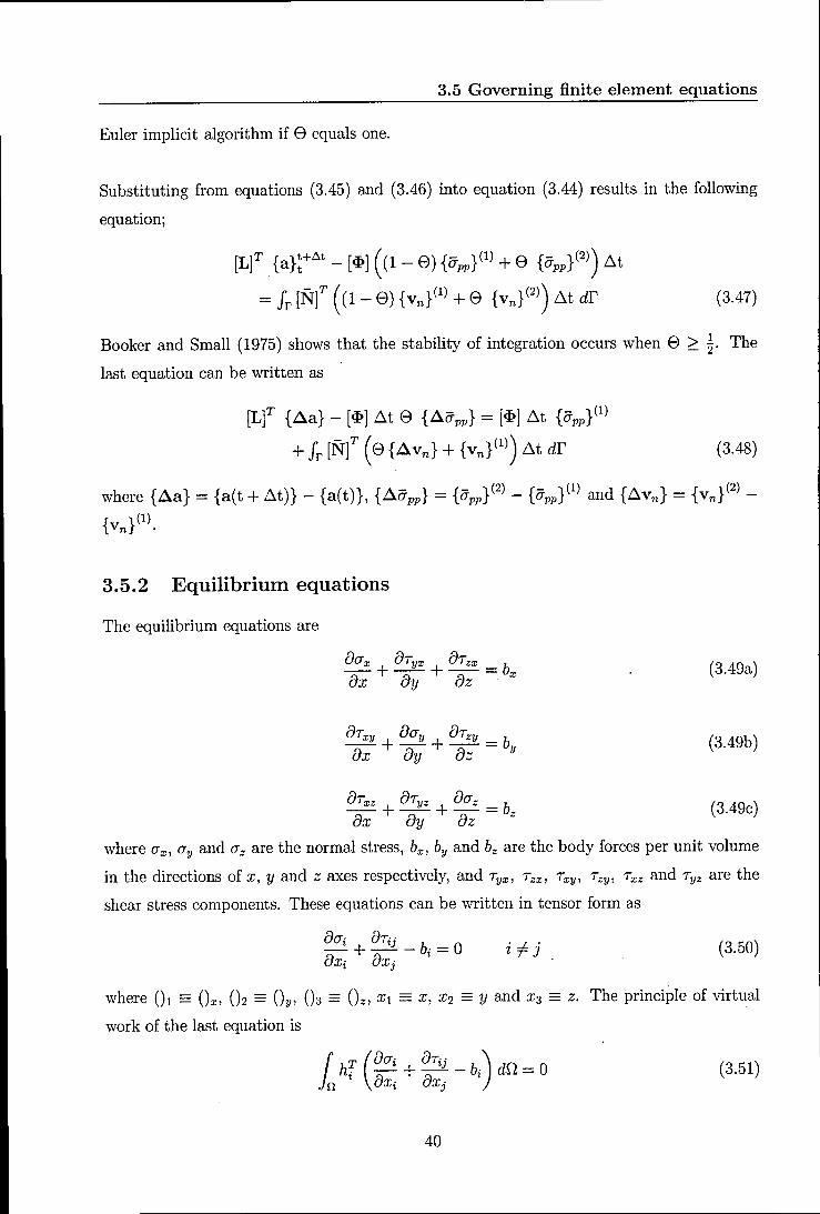
3.5 Governing finite element equations
Euler implicit algorithm if e equals one.
Substituting from equations (3.45) and (3.46) into equation (3.44) results in the following
equation;
[L]T {a}!+llt_[<I>] ((1-e){<7pp }(l) +8 {O'pp}(2»)~t
= Ir [N{ ((1 - 8) {Vn}(l) + 8 {Vn }(2») ~t dr (3.47)
Booker and Small (1975) shows that the stability of integration occurs when 8 ;::: ~. The
last equation can be written as
[Lf {Aa} - [<I>] ~t e {AO'pp} = [<I>] ~t {o-pp}(l)
+ Ir [:N{ (8 {Avn} + {Vn}(l») ~t dr (3.48)
where {Aa} = {a(t + ~t)} - {a(t)}, {A<7pp } = {O'pp}(2) - {o-pp}(l) and {~vn} = {Vn }(2) -
{Vn}(l) .
3.5.2 Equilibrium equations
The equilibrium equations are
(3.49a)
OTxy oay OTzy b -+-+-= ox oy oz y
(3.49b)
(3.49c)
where ax , ay and az are the normal stress, bx , by and bz are the body forces per unit volume
in the directions of x, y and z axes respectively, and Tyx , Tzx , Txy , Tzy , Txz and Tyz are the
shear stress components. These equations can be written in tensor form as
oai OTij b - 0 -+-- i-OXi OXj
(3.50)
where 01 = Ox, (h = Oy, 03 == Oz, Xl = X, X2 == Y and X3 == z. The principle of virtual
work of the last equation is
(3.51)
40

3.5 Governing finite element equations
where hi are arbitrary functions and called weighting functions. On applying the divergence
theorem to the last equation results
r (8h i )T r T - in 8Xi ai dO. + ir hi ai ni dr
1 (~:;) T Tij dO. + i hf Tij nj dr
-1 hf bi dO. = 0
\\Then hi is identified as the displacement (i.e. hi = Ui) then
8h i
therefore equation (3.52) becomes
-=Ei 8Xi
(3.52)
(3.53)
-1 Ef ai dO. + i uf(ai ni + Tij nj) dr -1 uf bi dO. = 0 (3.54)
The last equation can be written in matrix form as
(3.55)
where {T} is a vector with components Ti = aini + Tijnj which are called 'tractions' and
the term fr { u} T {T} dr represents the work done by these tractions on the boundary of
the continuum. In order to emphasise in the virtual work principle that the strains are
not necessarily caused by stresses, but can be arbitrary as long as they are compatible, it
is common to denote the virtual strains and displacements by superscript *, i.e. {E*} and
{u*}. Hence, like the relations (3.31) and (3.36) the following relations are considered
{u*} = [Nu] {a*} and {E*} = [B] {a*} (3.56)
and equation (3.54) is written in the incremental form as
The linear elastic stress-strain relation for the material is \VTitten as
{a'l = [D] {E} (3.58)
where {a/} is the effective stress and the components of tensor [D] are defined by equation
(3.17). On using relations (3.32), (3.36) and (3.58) the following equation
(3.59)
41

3.6 GeoFEAP and GeoFEAP2
can be written as
(3.60)
Substituting equations (3.56) and (3.60) into equation (3.55) results in
{a*f (L [Bf [D] [B]dO) {Aa} + {a*}T (L [Bf {m} [N-pp] dO) {Aa}
= {a*f (1 [Nuf {AT} elf + L [Nuf {Ab} dO) (3.61)
{a*}T can be cancelled to give
where [K] is the stiffness matrix, defined as
[K] = L [B]T [D] [B] dO (3.63)
Equations (3.49a) and (3.62) are used to establish a solution at time t+~t from the solution
at time t. Thus the solution can be marched forward in time from t = o. In summarising,
these equations can be written as
(3.64)
where
(3.65)
and
{F2 } = [f)?]llt {upp}(l) + 1 [Nu]T (e {Avn} - {vn}(l)) llt dr (3.66)
where {F1} and {F2 } are vectors that can be evaluated from loads and solution values at
time t.
3.6 GeoFEAP and GeoFEAP2
3.6.1 Capabilities of GeoFEAP
GeoFEAP is a general purpose geotechnical finite element program for static analysis of
two-dimensional nonlinear axisymmetric soil-structure interaction problems developed at
the University of California at Berkeley by Espinoza et al. (1995). This program is based on
the well-validated general purpose finite element analysis program (FEAP) and the earlier
42

3.6 GeoFEAP and GeoFEAP2
version of FEAP is described in Zienkiewicz and Taylor (1989, 1991).
GeoFEAP was modified to provide additional capabilities for solving problems of interest to
geotechnical engineers. A FE analysis from pre-processing to post-processing is prescribed
by a variety of macro commands, which allow the user to perform an analysis in a batch
mode, an interactive mode or a combination of these modes. The program also includes
a graphical processor to allow the analyst to readily visualise the results even during the
analysis. This processor includes the capabilities of displaying meshes, stress/strain contours
and displacement vectors. Figure 3.6 shows the general GeoFEAP layout. This flexibility
allows the inclusion of a wide variety of solution schemes, which can be essential when solving
problems using different non-linear stress-dependent soil constitutive models.
GeoFEAP I ~
I GeoFEAP control card I ~
Commands for creating a FE model (Mesh commands):
Geometry Mesti output file
Initial and boundary conditions
Material +----
Element parameters library
J Commands for solutions
(Batch or interactive commands)
~ Commands for plotting
(Plot commands)
Figure 3.6: General GeoFEAP layout.
Four types of elements are implemented within the GeoFEAP element library:
(1) 2-noded bar element,
43

3.6 GeoFEAP and GeoFEAP2
(2) 2-noded beam element,
(3) 4-noded interface element, and
(4) 3,4,5, 6, 7, 8 and 9-noded soil elements.
A combination of one or more element types allows for realistic analysis of earth embank
ments, retaining walls and reinforced soil slopes.
The program can model a variety of geotechnical problems with different soil models. Presently,
the structural bar and beam elements are modelled as a linear isotopic elastic material. In
terface elements may be used to model the non-linear behaviour of soil-structure interfaces
or shear planes within a soil mass (Clough and Duncan, 1969; Goodman et al., 1968). The
soil response can be represented by:
1. non-linear stress-dependent incrementally elastic hyperbolic model (Duncan et al.,
1980),
2. Drucker-Prager's model assuming an elastic-perfectly plastic material,
3. non-linear stress-dependent elasto-plastic model (Lade and Duncan, 1975), or
4. modified cam-clay model (Roscoe and Burland, 1968).
To solve non-linear governing equations, the Newton-Raphson technique is used to find a
solution which satisfies the global equilibrium of the analysed system. Both drained and
undrained analyses can be performed.
3.6.2 Limitations of GeoFEAP
To get more accurate results, the simultaneous interaction of soil and structure have to be
modelled, as explained in Section 1.3. GeoFEAP has the following limitations:
1. It is only a 2D axisymmetric program.
2. Shell elements are not implemented. However, a shell element is needed to model the
cooling tower shell.
3. The program does not model 3D soil-structure interaction problems.
4. It deals with the static analysis soil-structure interaction only.
44

3.7 Conclusion
3.6.3 New features programmed into GeoFEAP
Regarding to the previous limitations of GeoFEAP on modelling the 3D soil-cooling tower
interaction, the following new features are programmed into GeoFEAP:
1. Extending the capabilities of GeoFEAP to model footings and soil, using first order
8-noded hexahedron element. The 3D simultaneous interaction of soil and structure
problems can be therefore investigated.
2. Extending the Drucker-Prager yield criterion to 3D and implementing it.
3. Computing the deviatoric stress and mean pressure, as the most parameters of impor
tance to geotechnical engineers and modellers.
4. Implementing 4-noded quadrilateral flat shell element based on discrete Kirchhoff's
quadrilateral plate bending element. This element is used to model the elastic be
haviour of curved structural which has one small dimension (a thickness normal to the
remaining surface coordinates) compared to the other dimensions of the surface. The
model is also formulated in terms of force resultants which are computed by integration
of stress components over the cross-sectional thickness of the shell.
5. Modifying this element to accommodate a temperature profile.
6. Incorporating the modelling of thermal aspects of soil-structure interaction in both 2D
and 3D.
After programming these new features, the software was modified and re-programmed, and
renamed "GeoFEAP". The soil-cooling tower-interaction using GeoFEAP2 are then investi
gated taking into consideration the temperature changes in the cooling tower. In addition,
the effect of the modelling method of soil-cooling tower-interaction are also studied, via the
idealisation of the structure and soil on the resulting parameters.
3.7 Conclusion
In this chapter, the 3D governing finite element equations for the soil have been derived.
The soil parameters, elasto-plastic behaviour and reasons for choosing the appropriate con
stitutive Drucker-Prager's model in this analysis have been described. In addition, the
governing finite element equations of soil-structure interaction have been presented. These
governing finite element equations and the Drucker-Prager's model have been modelled in
45

3.7 Conclusion
GeoFEAP2. The Drucker-Prager's model requires two parameters; one defines the cohesion
(shear strength), and the second defines the dependence on the confining pressure, related
to the angle of friction in soil mechanics.
46

CHAPTER 4
Validation of the Software for Soil
Model
4.1 Overview
The aim of this chapter is to validate the new software (GeoFEAP2) when modelling the soil
structure interaction, as discussed in Chapter 3, for elastic and elasto-plastic soil behaviour.
This validation will be performed for one- and two- horizontal and vertical soil layers in
two and three dimensions with different types of elements and loads. The investigated
materials in this chapter are assumed to be homogenous, isotropic and have constant physical
properties.
4.2 Elastic behaviour of soil
In this section, the elastic behaviour of soil has been investigated to validate the software.
The soil is assumed to comprise one- and two- horizontal and vertical layers. It has been
investigated in 2D and 3D and modelled with 3-noded triangle and 4-noded quadrilateral
elements. Although the elastic type of model may not provide an accurate representation
of the actual behaviour of the soil, a number of geotechnical problems can be analysed
successfully with this soil model. The elastic soil model also allows the analyst to compare
the results with closed-form solutions available for some linear elastic problems (e.g. Poulos,
1967; Poulos and Davis, 1974).
47

4.2 Elastic behaviour of soil
4.2.1 2D circular flexible footing: 4-noded quadrilateral elements
The following example simulates the response of a soil undergoing an external surface load
to compare with the original example by Poulos and Davis (1974). Figure 4.1 shows the ge
ometric and stratigraphic characteristics of this problem. The corresponding finite element
mesh of 4-noded quadrilateral elements, comprising 140 elements and 165 nodes, has been
defined taking advantage of symmetry, as shown in figure 4.2. The mesh on the left side of
the symmetric line is considered for this example. The boundary conditions for the mesh are
as follows: the outer vertical boundary is restrained in the x-direction and is free to move
in the v-direction. The base of the layer is restrained in both x and y directions. The soil's
elastic properties are assumed to be Young's modulus of 180,000 lb/ft2 and Poisson's ratio
of 0.4 with an applied force of 1500 Ib/ft2. Imperial units have been used in order to be able
to compare with the original example by Poulos and Davis (1974).
Figure 4.3 shows the resultant displacement vector plot. Each vector represents the magni
tude (by its length) and the direction (by its orientation) of the displacement. The relative
magnitude of each of the vectors and their orientation clearly indicate the mechanism of
failure as shown in figure 4.4 which shows the settlement contour in the v-direction. It
can be seen from these figures that the displacements and contours decrease with depth and
away from the load as expected, which agrees with Poulos and Davis (1974). It is found that
the vertical displacement of a point just beneath the edge of the loading strip, i.e. at the
solid circled node, is 0.072 ft. The percentage error of this result is therefore zero compared
with the closed-form elastic solution, which is 0.072 ft Poulos and Davis (1974).
It. le 20ftl ·1
1500nl/ft!
~ ~ ~ ~ ~ I
E 11
(')
sr I~
x x f x x ·1 I
100ft
Figure 4.1: Geometric and stratigraphic characteristics for problems 4.2.1, 4.2.3 and 4.2.4.
48

25 ..... 1! Le; @ C\I
~
~
~
~
'0(
4.2 Elastic behaviour of soil
~
~
~
~ ~~ Q Q Q Q Q
[email protected]=15ft 2@5ft=1Oft [email protected]=25ft
Figure 4.2: Finite element mesh for problem 4.2.1.
"'''/~~#
Figure 4.3: Displacement resultant vector for problem 4.2.1.
49
<t. i

4.2 Elastic behaviour of soil
Total vertical displacement (ft)
1---'---'-+ -1.0SE-01 -8.S8E-02 -S.72E-02 -4.7SE-02 -2.79E-02 -8.27E-03
Current View Min = -1.2SE-01 ft X = 5.00E+01 ft Y = 3.00E+01 ft
Max = 1.14E-02ft X = O.OOE+oOft Y = 3.00E+01 ft
Figure 4.4: Settlement contours in the y-direction for problem 4.2.1.
4.2.2 2D circular flexible footing: 3-noded triangle elements
The problem considered in this section is a linear elastic drained soil layer of finite depth
subject to a uniform circular flexible footing with a radius of 4 m to compare with the orig
inal example by Poulos (1967) and Harr (1966). The corresponding finite element mesh of
this problem has been defined taking advantage of symmetry, as shown in figure 4.5. As
shown in this figure, the mesh consists of 80 elements and 54 nodes with 3-noded triangle
elements where the outer vertical boundary is restrained in the x-direction and is free to
move in the y-direction. The base of the layer is restrained in both x and y directions.
Young's modulus for the elastic soil layer is equal to 3 x 10³ kPa, with Poisson's ratio of 0.25
and an applied pressure of 30 kPa.
Figures 4.6 and 4.7 show the displacement resultant vector and settlement contour in the
y-direction respectively. It can be seen from these figures that the displacements and
contours decrease with depth and away from, the load as expected. The calculated vertical
displacement at the center, i.e. at node 6, and edge of the applied pressure, i.e. at node
18, are 54.2 mm and 32.0 mm, respectively. Poulos (1967) presented a theoretical solution
which gives a central displacement of 55 mm for a layer of the same thickness. In addition,
Harr (1966) presented an approximate solution, which gives a foundation edge settlement of
50

4.2 Elastic behaviour of soil
31 mm. The percentage errors are therefore 1.4% and 3.0% compared with Poulos (1967)
and Harr (1966) respectively.
~
I !30kPa
4@2m=Bm 4m Bm 2@10m=20m
Figure 4.5: Finite element mesh for problem 4.2.2.
1
Figure 4.6: Displacement resultant vector for problem 4.2.2.
Figure 4.7: Settlement contour in the y-direction for problem 4.2.2.
51
-i.84E-02 ·U8E.Q2 -3.09E.Q2 -.2.31E-02 ·1.S3E.Q2 ~7A9E-03
Mu- 2.99E~ft X-2.00E-t01ft Y·8.00E+ooft

4.2 Elastic behaviour of soil
4.2.3 Effect of Young's modulus on the settlement of 2D
axisymmetric circular footing on two horizontal soil layers
The response of two horizontal soil layers subject to an external circular footing has been
investigated in this section. Figures 4.1, 4.2 and 4.8 show the problem in question. In figure
4.2, the corresponding finite element mesh of 140 4-noded quadrilateral elements and 165
nodes has been presented, taking advantage of symmetry. It should be noted, as shown in
figure 4.8, that h = a = 10 ft, Eh! and Eh2 are Young's modulus of soil layers hI and h2
respectively and lJj,! and lJj,2 are Poisson's ratios of soil layers hI and h2 respectively, where
Eh! = 180,000 x Ah! Ib/ft2, Eh2 = Ah2 x 180,000 Ib/ft2 and lib! = lJj,2 = 0.4, where Ah! and
Ah2 are integer constants assumed as follows:
Ahj = 1 and 1 ~ Ahi ~ 50 such that EEhi = Ahi where i,j = 1,2 and i i= j (4.1) 'hj
The boundary conditions for the mesh are the same as explained in Section 4.2.1 with an
applied force of 1500 Ib/ft2.
a=1Oft j IC •
[) 16
<l
[)91 O~~
[) ~
~ ~ ~ ~ ~ ~ ~ ~
IC 50ft
Figure 4.8: Finite element mesh for problem 4.2.3.
soil layerh. ~l?VhJ
h=10ft
soil layerh2
Eh"Vh,
20ft
Figure 4.9 shows the vertical displacement of a point just beneath the edge of the loading
strip, i.e. at node 161, with
1 < Ehi < 50 where - Ehj -
i,j=1,2
52
and i =1= j (4.2)

4.2 Elastic behaviour of soil
It is noted that the vertical displacement at node 161, where? increases, is greater than h2
the vertical displacement at node 161, where? increases, and it decreases as ~Eh or? hi h2 hi
increases (Poulos and Davis, 1974). It should be also noted that the vertical displacement
at node 161, when Ehl = Eh2 , is equal to, as expected, 0.072 ft as discussed in Section 4.2.1.
~.01
~ ~.03 c: -.;; C! ~ ~.04
i c ~.05
I ~.08
~.07
~·080 5 10 15 20 25 30 35 40
~ /Eh & Eh /Eh t 2 1 2
Figure 4.9: Vertical displacement (ft) at node 161 as a function of Ehl/Eh2 and E h2 /Ehl .
Figures 4.10 and 4.11 show the settlement at the interface level, i.e. at y = 20 ft where the
nodes are numbered 91 to 105 as seen in figure 4.8, between the two soil layers of the elastic
soil when ~ = 1, 10, 20, 30, 40 and 50 where i, j = 1,2 and i 1= j. It is noted that the J
maximum modulus of the vertical settlement occurs at the central line and as expected it
decreases as :2l.EEh or? increases. In addition, h2 hi
(4.3)
where i, j = 1, 2, i 1= j, k = 1, 10,20,30, l = { ~ as k = {I otherwise.
However, the vertical settlement at the central line decreases very rapidly from ~h2 = 1 to hi
10, i.e. when the strength of soil layer h2 is greater than the strength of soil layer hI in this
range of EEh~ , and then decreases slowly from? = 10 to 30 and becomes a constant in the hi hi
range 30 to 50. This means that the major affected range for changing the ratio? is 1 to hi
10 and there is no effect when this ratio is grater than 30.
53
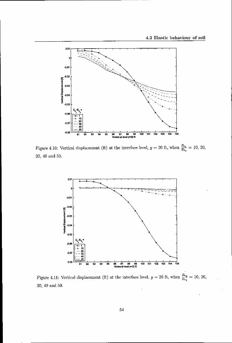
-0.08
-0.07
~~. , . -+- 1 ·+·10 ·_·20 - - 30 .... 40 -so
4.2 Elastic behaviour of soil
-O.~~~~~~L-~ __ ~~L-~ __ ~ __ L-~ __ ~L-L--L __ ~~ 91 92 93 94 95 96 97 98 99 100 101 102 103 104 105
Nodes at level yz20 11
Figure 4.10: Vertical displacement (ft) at the interface level, y = 20 ft, when? = 10, 20, 112
30, 40 and 50.
-0.01
g -0.02
"C! ~ 8 -0.03
i c 1-0·04
-0.05
-0.06
-0.07
~~. . , -+- 1 .+ 10 -·20
- - 30 ... 40 -so
-0.08 ~=='..l...---' __ -'--__ .L--': __ -'-__ '--L __ -'-L-L-~ __ ~--' __ .-J 91 92 93 94 95 96 97 98 99 100 101 102 103 104 105
Nodes a11eve1 y=20 11
Figure 4.11: Vertical displacement (ft) at the interface level, y = 20 ft, when? = 10, 20, hI
30, 40 and 50.
54

4.2 Elastic behaviour of soil
Figures 4.12 and 4.13 show the settlement at y = 20 ft for? = ? = 10 and 50 respectively. h2 hi
As shown in these figures, the modulus of the vertical settlement, as expected, decreases
rapidly when ~E~h = ~Eh because the volume of soil layer h1 is two times of soil layer h2 • h2 hi
0.01
0 0
.0.01
g 'i! ~ .0.02 5 .. 15. .!! C
~ .0.03
~
.0.04
91 92 93 94 95 96 97 98 99 100 101 102 103 104 105 Nodes at level y=20 ft
Figure 4.12: Vertical displacement (ft) at the interface level, y = 20 ft, when ~hi = ? = 10. h2 hl
0.01 r:--r-r----.--,---.-..,----,--r--.----.-,--,-..,-----,--,
o
.0.01
g 1i E .0.02
i c ~ .0.03
~
.0.04
o
.0.06 '-=7.=~~~_7--:~__=_--:':-_!:_---=:__:7:---:-:-::__-:-:--:7:___::'--:-! 91 92 93 94 95 96 97 98 99 100 101 102 103 104 105
Nodes at level y=2O ft
Figure 4.13: Vertical displacement (ft) at the interface level, y = 20 ft, when? = ? = 50. h2 hl
55
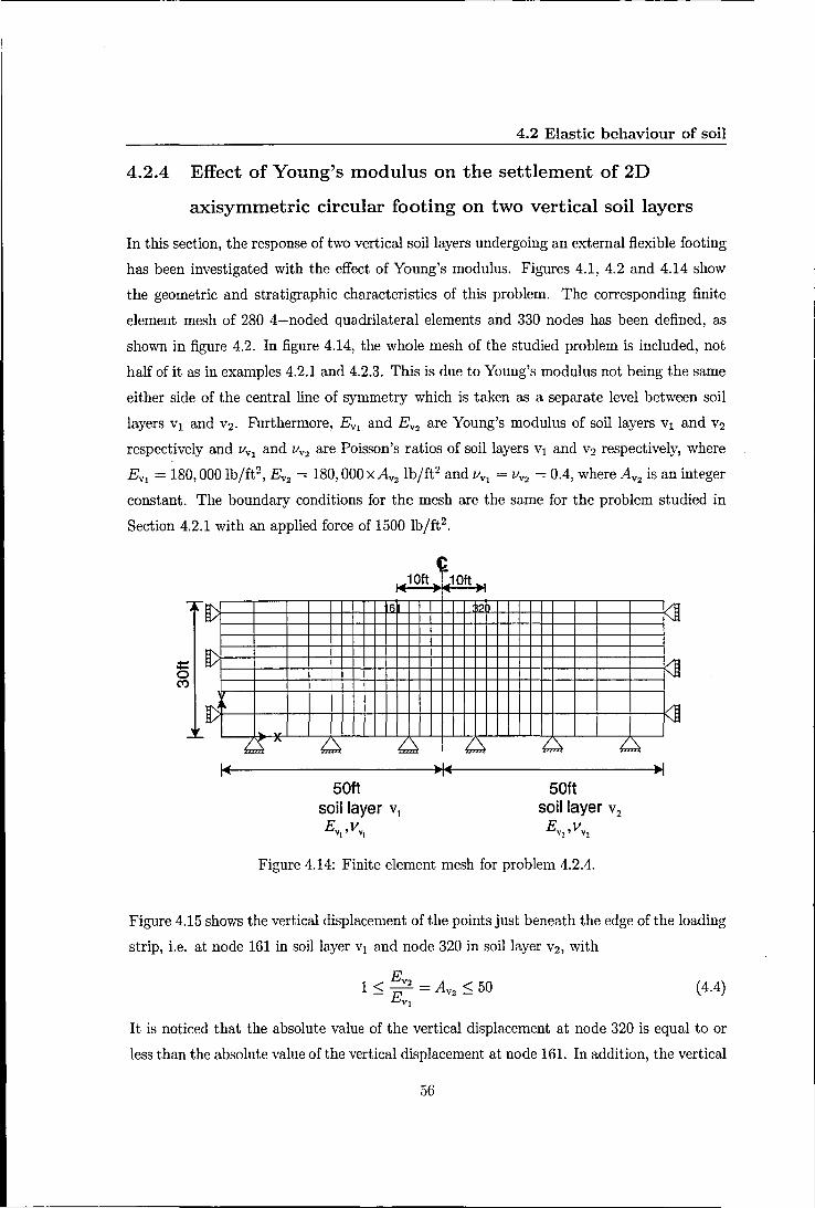
4.2 Elastic behaviour of soil
4.2.4 Effect of Young's modulus on the settlement of 2D
axisymmetric circular footing on two vertical soil layers
In this section, the response of two vertical soil layers undergoing an external flexible footing
has been investigated with the effect of Young's modulus. Figures 4.1, 4.2 and 4.14 show
the geometric and stratigraphic characteristics of this problem. The corresponding finite
element mesh of 280 4-noded quadrilateral elements and 330 nodes has been defined, as
shown in figure 4.2. In figure 4.14, the whole mesh of the studied problem is included, not
half of it as in examples 4.2.1 and 4.2.3. This is due to Young's modulus not being the same
either side of the central line of symmetry which is taken as a separate level between soil
layers Vl and V2' Furthermore, EYI and E Y2 are Young's modulus of soil layers Vl and V2
respectively and lIYl and lIV2 are Poisson's ratios of soil layers VI and V2 respectively, where
EYI = 180,000 Ib/ft2 , EY2 = 180,000 x AY2 Ib/ft2 and lIYl = lIY2 = 0.4, where AY2 is an integer
constant. The boundary conditions for the mesh are the same for the problem studied in
Section 4.2.1 with an applied force of 1500 Ib/ft2.
,
t> 16 12 KD
t> ~
[j ~ ~" ~ ~ ! ~ ~ ~
50ft 50ft soil layer VI soil layer v 2
EV1'VVl EV2 ,vV2
Figure 4.14: Finite element mesh for problem 4.2.4.
Figure 4.15 shows the vertical displacement of the points just beneath the edge of the loading
strip, i.e. at node 161 in soil layer Vl and node 320 in soil layer V2, with
1 EY2 - A < ~O ~ E - Y2 - i) YI
(4.4)
It is noticed that the absolute value of the vertical displacement at node 320 is equal to or
less than the absolute value of the vertical displacement at node 161. In addition, the vertical
56

4.2 Elastic behaviour of soil
displacement at node 320 increases more rapidly than the vertical displacement at node 161
in the range 1 :::; AV2 :::; 5 and then both curves increase slowly in the range 5 < AV2 :::; 50
such that the difference between these curves is big. The vertical displacement at node 161,
in soil layer Vl, is 25 times ofthe vertical displacement at node 320, in soil layer Vl. However,
it is constant in this range, i.e. 5 < AV2 :::; 50. It should be also noted that, when BVl = EV2 '
the vertical displacement at node 161, as expected, is equal to the vertical displacement at
node 320 = 0.072 ft as discussed in Section 4.2.1.
-0.01
~ -0.02 Pl '" ~ -0.03
~ ! -0.04 ~
~ a. -0.05 .!!l o
~ ~ -0.06
node number
I-*- 16~ -€>- 32
-0.08'-----'----'----'--"----'----'-----''----'------'----' o 5 10 15 . 20 25 30 35 40 45 50
EIE v v 2 ,
Figure 4.15: Vertical displacement at nodes 161 and 320 [ft] as a function of ~E~v • VI
Figures 4.16 to 4.20 show the settlement contours in the y-direction when? = 1, 20, 50, VI
70 and 100 respectively. The symmetric results (contours) of the vertical displacement have
been noticed in figure 4.16 when? = 1 and from figures 4.17 to 4.20, as e>.-pected, the VI
contours of the vertical displacement are non-symmetric although the two soil layers have
been affected by equal loads. In addition, these contours decrease as AV2 increases, i.e. when
soil layer V2 becomes stronger than soil layer Vl. This means that as AV2 increases as soil
layer V2 acts as a solid material which affects the behaviour of soil layer Vl as well. This
results that the vertical displacement contours being concentrated in the weaker soil layer
57

4.2 Elastic behaviour of soil
1-"""":''''''''':'4 ·1.oeE~1 -8.68E~2
-6.72E~2
-4.76E~2
·2.79E~2
-8.27E~3
Current v_ Min = ·1.28E·Ol It X • 5.00E+Ol It Y • 3.00E+Ol It
Max= 1.14E-D21t X= 1.00E+021t Y = 3.00E+01 It
Figure 4.16: Settlement contour in the y-direction for problem 4.2.4 when? = l. VI
Total vertical displacement (ft)
1--'-""'-""'--+ -5.67E~ h'i'_!'!'im -4.81E~2 F=~ -3.55E-ll2
·2.4BE~
·1.42E~
-3.53E-ll3
Cu""ntV_ Mln = -8.74E-ll2 It X - 4.25E+01 It Y-3.00E+011t
Max· 7.12E-ll31t X·O.OOE+OO1t Y-3.00E+011t
Figure 4.17: Settlement contour in the y-direetion for problem 4.2.4 when ~EEv = 20. VI
Total vertical displacement (ft)
1--'-""'-""'--+ -5.4SE.Q2
~~a -4.43E.Q2 p -3.42E.Q2
·2.41E~
·1.40E~
-3.86E-ll3
Cu""ntV_ Min· -6.4BE-ll2 It X • 4.25E+01 It Y-3.00E+011t
Max = 6.26E-ll3 It X-O.OOE+oo1t Y = 3.00E+01 It
Figure 4.18: Settlement contour in the y-direction for problem 4.2.4 when? = 50. VI
58

4.2 Elastic behaviour of soil
Total vertical displacement (ft)
f..--''''-''4 -S.40E~
~~.-4.40E~ F" -3.40E~ ·2.40E~
-t.39E~
-3.93E.Q3
CunentV_ Mln = -8.40E~ It X-4.25E+Ollt Y • 3.00E+Ol It
Max' 6.08E~3 It X • O.OOE+OO It Y-3.00E+Ol It
Figure 4.19: Settlement contour in the y-direction for problem 4.2.4 when? = 70. Vl
Total vertical displacement (ft)
f----4 -S.36E~ -4.37E~
-3.38E~
-2.38E~
-1.39E~
-3.99E.Q3
CunentV_ Mln = -8.35E~ It X· 4.25E+Ol It y. 3.00E+Ol It
Mu = S.B4E.Q3 It x - O.OOE+OO It Y-3.00E+Ol It
Figure 4.20: Settlement contour in the y--:direction for problem 4.2.4 when ~:~ = 100.
59

4.2 Elastic behaviour of soil
4.2.5 3D soil-structure interaction with a column
The aim of this section and Section 4.2.6 is to validate the software and model for the 3D
soil-structure interaction undergoing an external load as a base for studying the 3D soil
cooling tower- interaction problem which will be investigated in Chapters 7 and 8.
Figure 4.21 shows the geometric and stratigraphic characteristics of a 3D soil-structure inter
action with a column having it's concrete footing sitting on the soil. The corresponding finite
element mesh, shown in figures 4.22 and 4.23, consists of 332 first order 8-noded hexahe
dron elements with 879 nodes where the column is modelled by a 2-noded bar element. The
boundary conditions for the mesh are as follows: the outer vertical boundary is restrained
in the x and y directions and is free to move in the z-direction. The base of the soil layer
is restrained in the x, y and z directions. The soil's and structure's elastic properties are
assumed to be Young's modulus of 104 kPa and 30 x 106 kPa, Poisson's ratio of 0.3 and
0.2, and a unit weight of 20 kN/m3 and 24 kN/m3 , respectively (Das, 2002; Hunt, 1984).
These parameters would be representative of clay and concrete. In addition, the column's
properties are assumed to be Young's modulus of 20 x 106 kPa and a cross section of 0.1 m2
with an applied force of 1000 kN in the opposite of the z-direction.
The displacement and stress results in the x, y and z directions have been found to be
symmetric around the central lines, as shown in figure 4.22. These results are the same at
the solid circled nodes. In addition, it is found, as expected, that Fz = Rz and Rx = Ry = 0,
where Fz is the applied force in the z-direction and Rx, Ry and Rz are the total reaction
in x, y and z directions respectively.
Figures 4.24 and 4.25 show the top view for the displacement contours at z = 5 m and
z = 4 m respectively while figure 4.26 presents a side view for the settlement contours in
the z-direction. It can be seen from these figures that the displacement contours decrease
with depth and away from the load as expected. In addition, the major settlement occurs
at the soil-structure interaction surface which is shown in figure 4.22. Figure 4.27 shows
the deviatoric stress values, which are defined by equation (3.22) and measured in kPa, as
a function of x and y, measured in m, at the soil-structure interaction interface, which is
shown in figure 4.22, before and after applying the load. The maximum deviatoric stress
value occurs, as expected, at the middle of this interface, as shown in figure 4.27, and is
equal to 494.8 kPa.
60

column 1000kN
z
x+------J
5rn
Figure 4.21: Geometric and stratigraphic characteristics for problem 4.2.5.

E Lt)
..; 11 E ~ ,.... @ Cl)
E "1E o~ I§? 11 N
E Lt)
..; 11 E ~ ,.... @ Cl)
E 'fI E ,.... (§) Lt)
IC
IC
[email protected]=4.5m
~
~ ~ ~ ~
4.2 Elastic behaviour of soil
soil-structure Interaction l..---- surface at z=5m
t-----t-----r.-T..
[email protected]=4.5m
Figure 4.22: Finite element mesh, top view, for problem 4.2.5.
E Cl)
11 E ,.... (§) Cl)
11
~E I§?~
"
[email protected]=4.5m
r- f-
l- f-
[email protected]=4.5m
Figure 4.23: Finite element mesh, side view, for problem 4.2.5.
62

4.2 Elastic behaviour of soil
Total vertical displacement (m)
~':---4 -5.11E-02 -4.26E-02 -3.41E-02 -2.56E-02 -1.70E-02 -8.52E-03
CurrenlV_ Min = -5.81 E-02 m x = 5.00E+OO m Y· 5.00E+OO m Z = 8.00E+OO m Max = O.OOE+OO m X = O.OOE+OO m Y = O.OOE+OO m Z = O.OOE+OO m
Figure 4.24: Settlement contours, top view, at z = 5 m in the z-direction for problem 4.2.5.
Total vertical displacement (m)
1----1 -5.11E-02 -4.26E-02 -3.41E-02 -2.56E-02 -1.70E-02 -8.52E-03
CurrenlV_ Min = -4.32E-02 m X = 5.00E+OO m Y = 5.00E+OO m Z = 4.00E+OO m Max = O.OOE+OO m x = O.OOE+OO m Y = O.OOE+OO m Z • O.OOE+OO m
Figure 4.25: Settlement contours, top view in the z-direction, layer hI - layer h2 interface,
i.e. z = 4 m, for problem 4.2.5.
63

1
4.2 Elastic behaviour of soil
Total displacement in z-direction (m)
j.i..:-.......;..":"";4 -5.11E-02
-4.26E-02 -3.41E-02 -2.56E-02 -1.70E-02 -8.52E-03
Current v_ Min = -5.81 E-02 m X = 5.00E+OO m Y = 5.00E+OO m Z = 6.00E+OO m Max = O.OOE+OO m X = O.OOE+OO m Y = O.OOE+OO m Z = O.OOE+OO m
Figure 4.26: Settlement contours, side view in the z-direction, for problem 4.2.5.
Oeviatoric stress [lcPa]
500
400
100
5.5
y[m]
~x[m]
Figure 4.27: Deviatoric stress values at the soil-structure interaction surface, shown in figure
4.22, before and after applying the load.
64

4.2 Elastic behaviour of soil
4.2.5.1 Two horizontal soil layers
The response of two horizontal soil layers subject to an external point load has been inves
tigated in this section. Figures 4.21, 4.22 and 4.28 show the problem in question, where Ehl
and Eh2 are Young's modulus of soil layers hI and h2 respectively and IJbI and lJh2 are Poisson's
ratios of soil layers hI and h2 respectively, where Eh! = 104 X Ah! kPa, Eh2 = 104 X Ah2 kPa
and 1Jb! = 1Jb2 = 0.3, where Ah! and Ah2 are integer constants. In the present analysis Ahl
and Ah2 are assumed as in equation (4.1). The properties of the other materials for this
problem and boundary conditions for the mesh are the same as for the problem studied in
Section 4.2.5.
E C')
11 E ~
@ C')
E Ii
E 10
11 E ~
@ 10
[email protected]=4.5m
r-r-r-r-
[email protected]=4.5m
layerh2 Eh,.Vh,
layer hi Ehl,Vh\
~I
Figure 4.28: Finite element mesh, side view, for problem 4.2.5.1.
Figures 4.29 to 4.33 show the displacement contour in the z-direction when ?=10, 20, h2
30, 40 and 50. It can be seen from these figures that the displacement in the z-direction
decreases as ? increases, i.e. when soil layer hI is stronger than soil layer h2. On the other h2
hand, figures 4.34 to 4.38 show the displacement contour in the z-direction when ~Eh =10, hi
20, 30, 40 and 50. It can be seen from these figures that the displacement in the z-direction
increases as ? increases, i.e. when soil layer h2 is more stronger than soil layer hI. hi
65

1
4.2 Elastic behaviour of soil
Total displacement in z-direction (m)
1-'-"':""';"':""';.... -2.12E-02
-1.76E-02 -1.41E-02 -1.0SE-02 -7.00E-03 -3.46E-03
CurrenlVrew Min = -2.32E-02 m X = 5.00E+OO m Y = 5.00E+OO m Z = 6.00E+OO m Max = 8.82E-05 m X = 3.00E+OO m Y = 4.50E+OO m Z = 5.00E+OO m
Figure 4.29: Settlement contours in the z-direction when? = 10 for problem 4.2.5.l. h2
1
Total displacement in z-direction (m)
1--'-;";";;'-+ -1.92E-02 ~""""",,,,,,,,",,d- -1.58E-02 "~E1i4 -1.24E-02
~.95E-03
-S.53E-03 -2.12E-03
CurrenlVrew Min = -2.11 E-02 m X = 5.00E+OO m Y = S.OOE+OO m Z = 6.00E+OO m Max = 1.29E-03 m X = 5.50E+OO m Y = 7.00E+OO m Z = 5.00E+OO m
Figure 4.30: Settlement contours in the z-direction when? = 20 for problem 4.2.5.l. h2
66

1
4.2 Elastic behaviour of soil
Total displacement in z-direction (m)
1-'----'--':""':'-+ -1.85E-02 -1.51E-02 -1.18E-02 ~.41E-03
-5.04E-03 -1.68E-03
Current v_ Min .. -2.04E-02 m X .. 5.00E+OO m Y .. 5.00E+OO m Z .. 6.00E+OO m Max" 1.69E-03 m X .. 5.50E+OO m y .. 7.00E+OO m z .. 5.00E+OO m
Figure 4.31: Settlement contours in the z-direction when? = 30 for problem 4.2.5.l. h2
Total displacement in z-direction (m)
1-'-'':''''':'':''''':'4 -1.82E-02 -1.48E-02 -1.15E-02 ~.14E-03
-4.80E-03 -1.45E-03
Current V_ Min .. -2.00E-02 m X .. 5.00E+OO m y • 5.00E+OO m Z .. 6.00E+OO m Max" 1.89E-03 m X .. 5.50E+OO m y .. 7.00E+OO m Z .. 5.00E+OO m
Figure 4.32: Settlement contours in the z-direction when? = 40 for problem 4.2.5.l. h2
67

1
4.2 Elastic behaviour of soil
Total displacement in z-direction (m)
~-'--""':"'-+ -1.80E-02
~§I§I~ -1.46E-02 Ill! -1.13E-02
'.Y,'/.''''4d'iJ -7.98E-03
-4.65E-03 -1.32E-03
Cunenl Vte!W Min = -1.98E-02 m X = 5.00E+OO m Y = 5.00E+OO m Z = 6.00E+OO m Max = 2.01 E-03 m X" 5.50E+OO m Y = 7.00E+OO m Z = 5.00E+OO m
Figure 4.33: Settlement contours in the z-direction when? = 50 for problem 4.2.5.l. Jh2
1
Total displacement in z-direction (m)
F:--"::::""::"::::""::"-j -2.85E-02
-2.38E-02 -1.90E-02 -1.43E-02 -9.51E-03 -4.76E-03
Cunenl Vte!W Mln = -3.18E-02 m X = 5.00E+OO m Y = 5.00E+OO m Z = 6.00E+{)O m Max = O.OOE+OO m X = O.OOE+OO m Y = O.OOE+OO m Z = O.OOE+OO m
Figure 4.34: Sett.lement contours in the z-direction when? = 10 for problem 4.2.5.l. hi
68

1
4.2 Elastic behaviour of soil
Total displacement in z-direction (m)
~c...:..:.:c...:..:.:4 -2.53E-02 -2.11E-02 -1.68E-02 -1.26E-02 .a.42E-03 -4.21E-03
CurrenlV_ Min = ·2.80E-02m X = 5.00E+oom Y·5.00E+OOm Z = 6.00E+OO m Max = O.OOE+OOm X = O.OOE+oom Y = O.OOE+OO m Z = O.OOE+OO m
Figure 4.35: Settlement contours in the z-direction when? = 20 for problem 4.2.5.l. hi
1
Total displacement in z-direction (m)
f-'--'-c...:..:.:--4 -2.38E-02 -1.98E-02 -1.59E-02 -1.19E-02 -7.93E-03 -3.96E-03
CurrenlV_ Mln = -2.62E-02 m X = 5.00E+OO m Y .. 5.00E+OO m Z = 6.00E+OO m Max = O.OOE+OOm X = O.OOE+OO m Y = O.OOE+OO m Z = O.OOE+OO m
Figure 4.36: Settlement contours in the z-direction when ~h' = 30 for problem 4.2.5.l. hi
69

1
4.2 Elastic behaviour of soil
Total displacement in z-direction (m)
f-=--'--f -2.29E-02 -1.91E-02 -1.53E-02 -1.14E-02 -7.63E-03 -3.82E-03
CurrentVrew Mln = -2.52E-02 m X = 5.00E+OO m Y • 5.00E+OO m Z = 6.00E+OO m Max = O.OOE+OO m X = O.OOE+OO m Y = O.OOE+OO m Z = O.OOE+OO m
Figure 4.37: Settlement contours in the z-direction when? = 40 for problem 4.2.5.1. hi
1
Total displacement in z-direction (m)
1---'---'-4 -2.23E-02 -1.86E-02 -1.49E-02 -1.12E-02 -7.43E-03 -3.72E-03
CurrentVrew Min = -2.45E-02 m X = 5.00E+OO m Y • 5.00E+OO m Z = 6.00E+OO m Max = O.OOE+OO m X = O.OOE+OO m Y = O.OOE+OO m Z = O.OOE+OO m
Figure 4.38: Settlement contours in the z-direction when? = 50 for problem 4.2.5.1. I
70

4.2 Elastic behaviour of soil
Figure 4.39 shows the vertical displacement contours at the interface level, i.e. at z = 4 m
and x = 5 m, when ? and ? = 10, 20, 30, 40 and 50, respectively. It is shown in figure h2 hi
4.39 that the vertical settlement decreases very rapidly from ? = 1 to 10, i.e. when the h2
strength of soil layer h1 is greater than the strength of soil layer h2 in this range, and then
decreases slowly from ~EEh = 10 to 50. However, figure 4.40 shows that the vertical settlement 1£
decreases rapidly from i?- = 1 to 10, i.e. when the strength of soil layer h2 is greater than hi
the strength of soil layer h1 in this range, and then decreases slowly from? = 10 to 50. hi
on A a; -0.01 ~ '" lil ~ -0.015 :s '" 5 ;;; -0.02
8 'il .~ -0025 'i' . N
oS til -0.03 E
~ g. -0.035 '6
~ ~ -0.04
.+ .. + .+ ...
-O.0450~--~--~2----3~--~4----~5----~6----7~--~8----~9--~10
Displacement [m] in y-direction
Figure 4.39: Vertical displacement [m] at level z = 4 m when? = 10, 20, 30, 40 and 50. h2
Or---'---~----r---'---~----~---r--~----.---~
Eh~ 4- I + 10 .- 20 - - 30
40 -50
-O.0450~--~--~2----3L---~4----~5----6L---~7----~8----L9--~10
Displacement [m] in v-direction
Figure 4.40: Vertical displacement [m] at level z = 4 m when EEh, = 10, 20, 30, 40 and 50. hi
71

4.2 Elastic behaviour of soil
This means that the affected range for changing the ratios of ? and ~E~h is between 1 to h2 hl
10. It should be noted that the settlement in the case of ? is bigger than the settlement - h2
of ~Eb because the soil volume in the first case is four times of the second case, as shown in hl
figure 4.28. This is the same conclusion obtained on investigating the 2D two horizontal soil
layers in Section 4.2.3.
Figure 4.41 shows the displacement contour in the z-direction of the same soil with the
same properties except that llb2 = 0.4999, i.e. soil layer h2 is assumed to be undrained being
loaded in the short term, where pore water is not allowed to drain from the soil sample
during loading, the increase in stress is carried by the pore water, called the excess pore
water pressure. It is ,vell-known that the standard displacement finite element formulation
of elastic problems fails when the material becomes incompressible, i.e. volume remains
constant, or Poisson's ratio v reaches 0.5, see equation (3.18). A simple method to side-step
this difficulty is to use Poissons ratio close to 0.5 but not equal to it. This strategy is widely
adopted in a number of commercial geotechnical finite element softwares (Phoon et al., 2003).
It can be seen from figure 4.41 that the displacement in the z-direction decreases at soil
layer h2' compared with figure 4.26, i.e. when llb2 = llb l and Eh2 = E hl , because VJ12 is bigger
than llbl .
1
Total displacement in z-direction (m)
r--:'-'-----t -3.79E.(J2 -3. 16E.(J2
-2.53E.(J2 -1.89E.(J2 -1.26E.(J2 -6.32E.(J3
CurrenlV_ Min = -4.27E.(J2 m x. 5.00E+OO m y .. 5.00E+OO m Z = 6.00E+{)O m Max = O.OOE+OO m x .. O.OOE+OO m y = O.OOE+OO m z· O.OOE+{)O m
Figure 4.41: Settlement contours in the z-direction when llb2 = 0.4999 for problem 4.2.5.1.
72

4.2 Elastic behaviour of soil
4.2.5.2 Two vertical soil layers
In this section, the response of two vertical soil layers undergoing an external point load
has been investigated. Figures 4.21, 4.22 and 4.42 show the geometric and stratigraphic
characteristics, finite element mesh in top and side views of this problem respectively. In
figure 4.42, EVI and EV2 are Young's modulus of soil layers VI and V2 respectively and VVI
and VV2 are Poisson's ratios of soil layers VI and V2 respectively, where EVI = 104 kPa,
EV2 = 104 X AV2 kPa and VVI = VV2 = 0.3, where AV2 is an integer constant. The properties
of the other materials for this problem and boundary conditions for the mesh are the same
for the problem studied in Section 4.2.5.
E 'fI E ,.... @ 10
,e
,e [email protected]=4.5m
layer v2
EV2 ,vV2
E C')
11 E ,.... @ C')
E 'ii
r-I--I--I-
.,e .'4' ., [email protected] [email protected]=4.5m
=1m
.'01 ., layer v! EV1,vvl
Figure 4.42: Finite element mesh, side view, for problem 4.2.5.2.
Figures 4.43 to 4.47 show the displacement contour in the z-direction when? = AV2 =10, VI
20, 30, 40 and 50. It can be seen from these figures that the displacement in the z-direction
decreases at soil layer V2 as AV2 increases, i.e. when soil layer V2 is more stronger than soil
layer VI. In addition, the contours of the vertical displacement are non-symmetric although
the two soil layers have been affected by equal loads. Furthermore, these contours decrease
as AV2 increases, i.e. when soil layer V2 becomes stronger than soil layer VI. This means that
as AV2 increases as soil layer V2 acts as a solid material which affects the behaviour of soil
73

4.2 Elastic behaviour of soil
layer Vl as welL This means that the vertical displacement contours being concentrated in
the weak soil layer Vl.
1
Total displacement in z-direction (m)
I-"-=:.:.;c....;.;.;:...-+ -2.04E-02
~!'m~t -1.70E-02 R~='+ -1.36E-02
-1.02E-02 -6.81E-03 -3.41E-03
CurrenlV_ Mln = -2.39E-02 m X = 4.50E+OO m Y .. 4.50E+OO m Z = 6.00E+OO m Max = O.OOE+OO m X = O.OOE+OO m Y = O.OOE+OO m Z = D.OOE+OO m
Figure 4.43: Settlement contours in the z-direction for problem 4.2.5.2 when AY2 = 10.
Total displacement in z-direction (m)
1-"-=---+ -1.58E-02
~~0Y:'7 -1.32E-02 ~=='4 -1.06E-02
-7.92E-03 -S.28E-03 -2.64E-03
CurrenlV_ Min = -1.85E-02m X .. D.DDE+OO m Y • 5.00E+OO m Z = 5.00E+OD m Max = D.DOE+OOm X = D.OOE+OO m Y = D.DDE+OO m Z = D.DDE+OD m
Figure 4.44: Settlement contours in the z-direction for problem 4.2.5.2 when AV2 = 20.
74

1 kN
4.2 Elastic behaviour of soil
Total displacement in z-direction (m)
~-'----+ -1.58E-02 -1.32E-02 -1.06E-02 -7.92E-03 -5.28E-03 -2.64E-03
Current v_ Min = -1.85E-02 m X '" O.OOE+OO m Y '" 5.00E+OO m Z = 5.!¥IE+OO m Max = O.OOE+OO m X = O.OOE+OO m Y = O.OOE+OO m Z = O.OOE+OO m
Figure 4.45: Settlement contours in the z-direction for problem 4.2.5.2 when AV2 = 30.
Total displacement in z-direction (m)
1-----'-\ -1.58E-02 -1.32E-02 -1.06E-02 -7.91E-03 -5.28E-03 -2.64E-03
Current v_ Min = -1.85E-02 m X'" O.OOE+OO m Y·5.00E+OOm Z = 5.00E+OO m Max = O.OOE+OO m X = O.OOE+OO m Y = O.OOE+OO m Z = O.OOE+OO m
Figure 4.46: Settlement contours in the z-direction for problem 4.2.5.2 when AV2 = 40.
75

4.2 Elastic behaviour of soil
Total displacement in z-direction (m)
j..:.-:----::...;4 -1.58E-02
~~;m. -1.32E-02 jl;i -1.06E-02
-7.91E-03 -5.28E-03 -2.64E-03
CurrenlV_ Mln = -1.85E-02 m X = O.OOE+OO m Y " 5.00E+OO m Z = 5.00E+OO m Max = O.OOE+OO m X = O.OOE+OO m Y = O.OOE+OO m Z = O.OOE+OO m
Figure 4.47: Settlement contours in the z-direction for problem 4.2.5.2 when AV2 = 50.
Figure 4.48 shows the displacement contours in the z-direction of the same soil with the
same properties except that V2 = 0.4999, i.e. soil layer V2 is assumed to be undrained, as
explained in Section 4.2.5.1. It can be seen from this figure that the displacement in the
z-direction decreases at soil layer V2, compared with the figure 4.26, Le when VV2 = VVl and
EV2 = EV1 , because VV2 is bigger than VV1'
4.2.6 3D soil-structure interaction for one-storey building
The following example extends the problem which has been investigated in Section 4.2.5
and the results will be compared with those obtained by Kocak and Mengi (2000). Figure
4.49 shows the geometric and stratigraphic characteristics of a one-storey building having
an elastic floor, which stands, at its corners on columns supported by rigid square footings.
The corresponding finite element mesh is shown in figures 4.50 (a),(b),(c) and (d) for top
view of soil, side view of soil, footings and floor respectively.
The boundary conditions for the mesh are as follows: the outer vertical boundary is re
strained in the x and y directions and is free to move in the z-direction. The base of the
soil layer is restrained in the x, y and z directions.
76

1
4.2 Elastic behaviour of soil
Total displacement in z-direction (m)
1----=--=4 -1.53E-02
~~~a -1.26E-02 ~ -9.84E-03
-7.0SE-03 -4.34E-03 -1.58E-03
CurrenlV_ Min = -1.81E-02 m X" O.OOE+OO m Y = 5.00E+OO m Z = 5.00E+OO m Max= 1.17E-03m X = 5.00E+OO m Y = 1.00E+01 m Z = 5.00E+OO m
Figure 4.48: Settlement contours in the z-direction when VV2 = 0.4999 for problem 4.2.5.2.
Young's modulus is assumed to be 104 kPa for the elastic soil and 20 x 105 kPa for the rigid
footings, columns and roof. Poisson's ratio is assumed as 0.2 for the elastic soil, rigid foot
ings, columns and roof (Kocak and Mengi, 2000). In addition, the column's cross section and
moment of inertia are assumed to be 0'.16 m2 and 0.00213 m4 respectively with an applied
force of 100 kN at point A, as shown in figure 4.49 (a).
Figure 4.50 (e) shows the vertical displacement contours at the roof. It is shown that,
as expected, the maximum value is at the load point, i.e. at point A. In addition, the
displacement value decreases as the total distance between any point in the roof and point
A increases. It is also found that the force at the point B is -99.2 kN, an error of 1.8%
compared with the value -97.4 kN obtained by Kocak and Mengi (2000) who proved that
the interaction between the footings may be ignored, with respect to the element forces, due
to symmetry of the structure.
77

21.Sm
(a)
Figure 4.49: (a) Geometric and stratigraphic characteristics for the soil-structure interaction problem consid
ered in Section 4.2.6 and (b) top view for this problem.
(b)
~ ~
tJj
[ .... .... (")
0"" CD ::r ~ .... o ~ '1
o ...., 00 o .... -

(a)
(b)
1« 4m 2.Sm '0
1.5m O.7Sm 025m =1m
4@ O.Sm =2m
o~ O.75m 1.5m .1m
4.2 Elastic behaviour of soil
~I
2.Sm 4m
E ..
E '" N
E '" ,.:
E i!! ci
.. .liE ~~ii
@EE vd'it
o~.§ "'ci"
~ E ~
E '" N
~-+---+-I I +t+++-+-IIIIII I IH-+ttttl 11111-+---11 4F--==-I-1 -----III;·
E 4@02Sm=lm
m et (c)
.11 10CO.3m=3m
(d) (e)
Total vertical displacement at rool (m) ,..-.....-,,-, -II.68E.oo r----, ·7.~1E.oo
-II.16E-03 -4.S2E-03 -l.67E.oo ·2.~-O3
·1.18E-03 7.12E-OS
Figure 4.50: Finite element mesh for the soil-structure interaction problem considered in
Section 4.2.6 for ( a) top view of the soil, (b) side view of the soil (c) top view of the rigid
footings, (d) top view of the roof, and (e) vertical displacement contours at the roof.
79

4.3 Elasto-plastic behaviour of soil
4.3 Elasto-plastic behaviour of soil
4.3.1 Introduction to the problem
One of the most critical parameters required by an engineer when designing shallow founda
tions is the bearing capacity of the underlying soil. For simple cases, either exact solutions,
or upper and lower bounds can be found when the soil behaves in an elasto-plastic manner.
However, for the majority of actual geotechnical situations, the assumptions made when de
riving plasticity solutions provide a very crude idealisation of reality. (EI-Hamalawi, 1997).
The prediction of collapse loads under plastic flow conditions can be a significant numerical
challenge to simulate accurately. The limiting load-bearing capacity of soil structures forms
one of the classic problems of geomechanics. There are essentially three types of solution
methods: limit equilibrium methods (e.g. Meyerhof, 1951; Terzaghi, 1943), slip-line field
methods (e.g. Prandtl, 1921; Sokolovskii, 1960; Wu, 1976) and limit analysis methods (e.g.
Boulbibane and Ponter, 2005; Griffiths and Fenton, 2001).
In this section, the problem under consideration will be determining the bearing capacity of
a single soil layer and upon which a flexible square smooth footing of width b and weight
q acts, as shown in figure 4.51. The flexibility property means that any loading is uniform
and can be represented by a surface surcharge pressure applied to the surface of the soil
immediately below the position of the footing, i.e. the force is applied in the y-direction. If
the footing is smooth, then the other boundary condition that must be applied to the nodes
under the footing is that the horizontal nodal forces are zero.
~ footing
1m
I E 1'1 0 501 .... i
I
I
40m
Figure 4.51: Geometric and stratigraphic characteristics for problem 4.3.
80
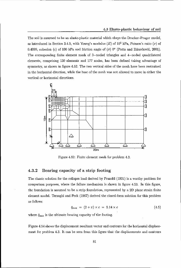
4.3 Elasto-plastic behaviour of soil
The soil is assumed to be an elasto-plastic material which obeys the Drucker-Prager model,
as introduced in Section 3.4.5, with Young's modulus (E) of 105 kPa, Poisson's ratio (v) of
0.4999, cohesion (c) of 100 kPa and friction angle of (cjJ) 0° (Potts and Zdravkovi6, 2001).
The corresponding finite element mesh of 3-noded triangles and 4-noded quadrilateral
elements, comprising 130 elements and 177 nodes, has been defined taking advantage of
symmetry, as shown in figure 4.52. The two vertical sides of the mesh have been restrained
in the horizontal direction, while the base of the mesh was not allowed to move in either the
vertical or horizontal directions.
Figure 4.52: Finite element mesh for problem 4.3.
4.3.2 Bearing capacity of a strip footing
The classic solution for the collapse load derived by Prandtl (1921) is a worthy problem for
comparison purposes, where the failure mechanism is shown in figure 4.53. In this figure,
the foundation is assumed to be a strip foundation, represented by a 2D plane strain finite
element model. Terzaghi and Peck (1967) derived the closed-form solution for this problem
as follows:
qma:x = (2 + 1T) x C = 5.14 x c (4.5)
where qma:x is the ultimate bearing capacity of the footing.
Figure 4.54 shows the displacement resultant vector and contours for the horizontal displace
ment for problem 4.3. It can be seen from this figure that the displacements and contours
81

4.3 Elasto-plastic behaviour of soil
decrease with depth and away from the load as expected, which agrees with the failure mech
anism, as shown in figure 4.53.
collapse load qmax = (2+Jr)c
Figure 4.53: Failure mechanism of a strip footing on a frictionless soil (Prandtl's wedge
problem).
Contours for the horizontal
displacement (m)
2.769E-03 2 2.423E-03 3 2.077E-03 4 1.731E-03 5 1.384E-03 6 1.03BE-03 7 6.922E-04 8 3.461E-04
Figure 4.54: Displacement resultant vectors and contours of the horizontal displacement for
problem 4.3.2.
Figure 4.55 shows the bearing capacity of a strip footing versus vertical displacement of the
footing. The final value of the bearing capacity is 516 kPa, an error of 0.01% compared to
the analytical solution 514 kPa, calculated using equation (4.5), which is negligible .
... I • ~ 3.15
8 L. 3
:I i 2.:
0 .•
0.01 0.02 0.03 D.IW 0.05 0.00 -...nd_lm]
Figure 4.55: Bearing capacity of a strip footing for problem 4.3.2.
82

4.3 Elasto-plastic behaviour of soil
4.3.3 Bearing capacity of a circular footing
If the foundation is circular, the solution to the problem considered in Section 4.3.2 becomes
as follows (Shield, 1955)
iimax = 5.69 x c (4.6)
Figure 4.56 shows the displacement resultant vector and contours for the horizontal displace
ment of problem 4.3 under the axisymmetric assumption where the loading is also symmetric
about the center line. It can be seen from this figure that the displacements and contours
decrease with depth and away from the load as expected, which agrees with the failure mech
anism, as shown in figure 4.53. Figure 4.57 shows the bearing capacity of a circular footing
versus vertical displacement of the footing. The· final value of the bearing capacity is 571
kPa, an error of 0.01% compared with the analytical solution 569 kPa, see equation (4.6),
which is negligible.
Contours for the horizontal
displacement (m)
1 1.688E-03 2 1.477E-03 3 1.266E-03 4 1.055E-03 5 8.43BE-04 6 6.32BE-04 7 4.219E-04 8 2.109E-04
Figure 4.56: Displacement resultant vectors and contours of the horizontal displacement for
problem 4.3.3.
I • ~ 8 r. 3
) ~ ;! 2
. - ..
0.01 0.02 0.03 0.04 0,05 o.D8 0.07 0.08 0.09 0.1 Mulmurn d~(ml
Figure 4.57: Bearing capacity of a circular footing for problem 4.3.3.
83

4.4 Conclusion
4.4 Conclusion
In this chapter, the new software (GeoFEAP2) has been validated when modelling the soil
structure interaction. 2D circular flexible footings have been analysed using quadrilateral
and triangular elements and the results compared well Vv1.th analytical solutions.
The effect of Young's modulus on the settlement of 2D a..xisymmetric circular footing has
been investigated when the soil is divided into two horizontal layers hI and h2 correspond
ing to the upper and lower layers of soil beneath the foundation respectively. It was found
that the vertical displacement decreases, as expected, with depth and away from the load.
In addition, the vertical displacement, where ::!!l.EEb increases, is higher than the vertical dis-h2
placement at the same point, where EEh, increases, and it decreases as ::!!l.EEh or EEh2 increases. ~ ~ ~
Moreover, the maximum modulus of the vertical settlement occurs at the central line and,
as expected, it decreases as ? or ~h' increases. Furthermore, the vertical settlement at the h2 hI
central line decreases very rapidly from ? = 1 to 10, i.e. when the strength of the lower hI
soil layer h2 is greater than the strength of the upper soil layer hI in this range of ?, and hI
then decreases slowly from? = 10 to 30 and becomes a constant in the range 30 to 50. hI
This means that the major affected range for changing the ratio? is 1 to 10 and there is hI
no effect when this ratio is greater than 30. Finally, the modulus of the vertical settlement
at the interface level, as expected, decreases rapidly when ? = ~E~h because the volume of h2 hI
soil layer hI is two tiines of the volume of soil layer h2.
The effect of Young's modulus on the settlement of 2D axisymmetric circular footing has
been modelled when the soil is divided into two vertical layers VI and V2, where EV2 2: Evl •
It was found that the vertical displacement at a node in the soil layer V2 is equal to the
vertical displacement at a node corresponding to the same position symmetrically in the soil
layer VI when EVI = E V2 ' However, the vertical displacement at a node in the soil layer
V2 is less than the vertical displacement at a node corresponding to the same position sym
metrically in the soil layer VI when EVI < E y2 • In addition, the vertical displacement at a
node corresponding to the same position symmetrically in the soil layer VI increases more
rapidly than the vertical displacement a node in the soil layer V2 in the range 1 :::; ? :::; 5 VI
and then increases slowly in the range 5 < ?- :::; 50. Moreover, the vertical displacement VI
at a node in soil layer VI, is 25 times of the vertical displacement at an equivalent node in
soil layer VI and is constant in this range, i.e. 5 < ?- :::; 50. The settlement contours in VI
the vertical direction when ?- = 1, 20, 50, 70 and 100 have been also discussed. It was VI
84

4.4 Conclusion
found that these vertical settlement contours decrease, as expected, with depth and away
from the load. In addition, these contours are symmetric when ? = 1 and, as expected, VI
non-symmetric when? > 1, although the two soil layers have experienced equal loads. VI
Furthermore, these contours decrease as :::2Ee,v increases. i.e. when the soil layer V2 becomes VI '
stronger than the soil layer V1. This means that as ~ increases as the soil layer V2 acts as
a solid material which affects the behaviour of the soil layer V1 as well. This results in the
vertical displacement contours being concentrated in the weak soil layer V1.
The 3D soil-structure interaction undergoing an external load has been investigated as a
base for studying the 3D soil-cooling tower-interaction problem. It was found that the dis
placement contours decrease with depth and away from the load as expected. In addition,
the major settlement occurs at the soil-structure interaction surface. Moreover, the displace
ment and stress results in the x, y and z directions have been found to be symmetric around
the central line. Furthermore, the maximum deviatoric stress value occurs, as expected, at
the middle of soil-structure interaction interface.
The response of the 3D two horizontal soil layers, h2 and h1 corresponding to the upper and
lower soil layers beneath the foundation respectively, structure interaction undergoing an
external load has been investigated. It was found that the vertical displacement decreases,
as expected, with depth and away from the load. In addition, the vertical displacement in
the vertical direction decreases as ? increases, i.e. when the lower soil layer h1 is stronger h2
than the upper soil layer h2' and increases as ~ increases, i.e. when the upper soil layer
h2 is stronger than the lower soil layer h1. Furthermore, the vertical displacement contours
at the interface level decrease very rapidly from? = 1 to 10, i.e. when the strength of the h2
lower soil layer h1 is greater than the strength of the upper soil layer h2 in this range, and
then decrease slowly from? = 10 to 50. However, the vertical settlement contours at the h2
interface level decrease rapidly from? = 1 to 10, i.e. when the strength of the upper soil hi
layer h2 is higher than the strength of the lower soil layer h1 in this range, and then decrease
slowly from? = 10 to 50. This means that the affected range for changing the ratios of hi
? and ? is between 1 to 10. It was also noted that the settlement when ? is bigger ~ ~ ~
than the settlement when ----"-EEh~ because the soil volume in the first case is taken as four times hi
of the soil volume in the second case. This is the same conclusion obtained on investigating
2D axisymmetric circular footing problem when the soil is divided into two horizontal layers.
If the upper soil layer h2 is assumed as undrained, the vertical displacement decreases at the
85

4.4 Conclusion
upper soil layer h2 because V},2 is bigger than /1j,1'
The response of the 3D two vertical soil layers, Vl and V2, structure interaction undergoing
an external load has been studied. It was found that the vertical displacement contours
decrease, as expected, with depth and away from the load. In addition, these contours in
the vertical direction decrease at the soil layer V2 as ~ increases, i.e. when the soil layer V2 VI
becomes stronger than the soil layer Vl. Furthermore, these contours are symmetric when
? = 1 and, as expected, non-symmetric when ? > 1, although the two soil layers have =VI -'-'VI
experienced equal loads. This means that as ? increases as the soil layer V2 acts as a VI
solid material which affects the behaviour of the soil layer Vl as well. This means also that
the vertical displacement contours will being concentrated in the weak soil layer Vl' This
is the same conclusion obtained on investigating 2D axisymmetric circular footing problem
when the soil is divided into two vertical layers. If the soil layer V2 is assumed as undrained,
the vertical displacement contours decrease at the soil layer V2 because VV2 is bigger than /lvI'
The 3D soil-structure-interaction for one-storey building undergoing an external load has
been modelled. It was found that the maximum value occurs, as expected, at the load point.
In addition, the displacement value decreases as the total distance between any point in the
roof and the load point increases, and the results compared well with the numerical solution
obtained by Kocak and Mengi (2000).
The bearing capacity of strip and circular footings have been studied. It was found that the
displacement resultant vector and contours for the horizontal displacement decrease with
depth and away from the load as expected, which agrees with the failure mechanism, and
the bearing capacities correspond well with the closed-form solution.
86

CHAPTER· 5
Implemented Shell Element
5.1 Overview
The four noded quadrilateral flat shell element is introduced in this chapter. Membrane
and bending elements based on Kirchhoff's assumptions are used for development of this
element, the stiffness matrix for it is then presented. In addition, thermal effects upon this
flat shell element are presented.
5.2 Introduction
A shell is a continuum which is bounded by two curved surfaces separated by the thickness
which may be constant or vary either gradually or abruptly therefore shells are amenable to
treatment by the continuum theory, in this case, the theory of elasticity. Two types are to be
considered; thin and thick shell. If the thickness is considerably smaller than the principal
radii of curvatures of the bounding surfaces then the shell is defined as a thin shell; if not, it
is termed thick. In addition, if each bounding surface is generated by the rotation of a plane
curve about a common axis, a shell of revolution is produced. Shell structures are one of
the most important structural elements, as they are widely used in a variety of engineering
applications. In this research, it has been assumed that the material from which the shell is
constructed is homogenous, isotropic and perfectly elastic so that Hooke's law can be used.
87

5.3 Types of shell elements
5.3 Types of shell elements
Shell elements are widely used to model the curved geometry of a structure. Shell elements
based on classical shell theory are very difficult to develop. Many simplifying approxima
tions are involved in the development. These types of elements are very efficient in modelling
the curved geometry of the structure. However, because of the complexities involved, the
alternative approach of modelling the structure with series of flat elements, which is simpler
and easier to implement, became more popular for the analysis of shell structures.
The main elements of shell structures include triangular and quadrilateral shells; low-order
and high-order shell elements; shallow and deep shells; flat and curved shell element; thick
and thin element; axisymmetric and sandwich shells. The axisymmetric shell structures,
generated by rotating a plane curve generator around an axis of rotation to form a circum
ferentially closed surface, have many applications such as hyperbolic cooling towers. These
structures are thin and the first attempt to apply the finite element analysis to them treated
the shell surface as being made up of flat plate elements (either triangle or quadrilateral in
shape) (Djoudi and Bahai, 2004). The two most widely adopted approaches in the finite
element analysis of general shells are (1) use of curved elements based on a suitable shell
theory and (2) approximation of the curved structure by an assemblage of flat shell elements.
Although the first plate bending element was introduced in 1961, elements which are ade
quate for general shell analysis only became available in the 1970s. The published literature
on modelling of plates and shells in the linear and non-linear regimes and their application
to dynamic or vibration analysis of structures has grown extensively. The long history of
gradual improvements in the design of finite shell elements has been reviewed by MacNeal
(1998) for the period 1956 to 1998, Yang et al. (2000) for the period 1985 to 2000 and Mack
erle (2002) for the period 1999 to 2001. Table 5.1 outlines the summary of plate and shell
elements development (Mackerle, 2002).
Needless to say that research on the design of plate and shell elements continues to this day.
However, numerous shell finite elements have been proposed and yet there is a consensus
that there are still difficulties in analysing general shell structures. In addition, it is difficult
to identify which shell elements are the most effective elements currently available, and how
to arrive at more efficient shell analysis procedures. It may be therefore fair to state that
no single theory has proven to be general and comprehensive enough for the entire range
88

5.4 Elastic shell theory
of applications (Chapelle and Bathe, 1998). Elements used in cooling tower shell will be
discussed in Section 2.6.
Table 5.1: Summery of plate and shell element development (Mackerle, 2002).
Element development Year
First membrane element 1956
First plate bending element 1961
Kirchhoff plate elements 1961 to 1970
Discrete Kirchhoff plate and shell elements 1969
First Mindlin shell element (8-noded quadrilateral) 1969
Reduced integration 1971
Local-global shell elements 1971
4-noded quadrilateral and 3-noded triangle 1976 to 1982
9-noded quadrilateral 1985 to 1990
High-order shell elements 1988 to recent
5.4 Elastic shell theory
5.4.1 Membrane theory
The membrane theory is based on a momentless plane stress system. It is applicable only if
the following physical conditions are met:
1. The properties of the shell's material are constant across the thickness of the shell.
2. The shell's bending rigidity is negligible compared to its membrane rigidity. In other
d th h 11 . d' 1 th" thickness 1 wor s, e s e IS excee mg y m, I.e. radii of curvature« .
3. The changes in radii of curvature are negligible.
5.4.2 Bending theory
Love (1888) established the bending theory of thin elastic shells for linear problems. In this
theory, the behaviour of thin shells are approximated by the following assumptions:
1. The material of the shell is isotropic and homogenous.
89

5.4 Elastic shell theory
2. The displacements are small.
3. The thickness of the shell is small compared with the radii of curvature of its middle
surface.
4. The stress components normal to the middle surface (shear and axial) are small com
pared to stresses tangent to the shell's surface and may be neglected in the stress-strain
relationship.
5. Normals to the middle surface remain normal to it and undergo no strain during
deformation. Hence, the transverse shear deformations are not taken into account.
The assumption that deflections are small, allows the assumption that the equations of
equilibrium with respect to both the original (undeformed) and deformed geometry are the
same. This, with Hook's law, ensures linear elastic behaviour. The physical interpretation
of assumption 5 is that the transverse shear deformations are not taken into account. This
is called Kirchhoff's assumption because the same assumption was proposed by Kirchhoff
(1876) to introduce the theory of plates.
Many researchers have tried to generalise Love's theory and this has led to the introduction
of additional theories of thin shell. One of these is the first order approximation theory in
which all of Love's original assumptions are preserved. The well-known work in this cate
gory was done by Reissner (1941). Reissner was the first to use the lines of curvatures to
derive the shell's theory equations based on Love's theory. Figure 5.1 shows the membrane,
bending and coupled stress of the shell.
Natural draught cooling towers are an effective and economic choice among all technical
solutions for the prevention of thermal pollution of natural water resources caused by heated
cooling water in various industrial facilities. Cooling towers are shells of double curvature
that resist applied forces primarily through in-plane membrane action. These shells can be
more than 150 m in height and 60 m in base diameter. These towers have at most a wall
thickness of about 20 to 25 cm. In general, both membrane and bending act~ons are present
in the shell. However, it should be noted membrane stresses are the most important stresses.
in the designing of a cooling tower shell (ACI-ASCE, 1977). Hence, the shell behaviour is seen
as a superposition of membrane and plate bending actions. Finite elements are constructed
by simply combining plate bending and plane stress stiffness matrices. This approach will
be discussed in Sections 5.5,5.6 and 5.7.
90

5.5 Membrane elements
+ membrane stress bending stress
coupled stress
Figure 5.1: Membrane, bending and coupled stresses in a shell element.
5.5 Membrane elements
5.5.1 Introduction
Membrane elements are used for analysing structures subjected to in-plane forces. These
elements are used to model the behaviour of shear wall, stiffened sheet construction, and
membrane action in shells. Assuming that the structure is in the xy plane, the displacements
at any point of the structure are u and v, the translation in the x and y directions, respec
tively. The stresses of interest are the normal stresses O'x and O'y and the shearing stress 7xy •
The normal stress in the direction perpendicular to the plane of structure is considered to
be zero.
Isoparametric elements are useful for modelling structures with irregular boundaries; since
these elements can have curved sides. They are formulated in the natural coordinate system
that maps the element geometry in terms of natural coordinates regardless of the orientation
of an element in the global coordinate system; however, the relationship between the two
systems must be used in the element formulation (Cook, 1995).
Irons (1966) introduced the concept of isoparametric elements in stiffness methods. Erga
toudis et al. (1968) developed shape functions to formulate the element stiffness matrix for
four noded isoparametric quadrilateral element. The four noded isoparametric quadrilateral
plane element is used to develop the quadrilateral flat shell element in this study.
91

5.5 Membrane elements
5.5.2 Elasticity constitutive model
Two dimensional elasticity problems typically involve structures that are very thin and the
loads are applied in the direction in the plane of the structure. Consider a structure in the
xy plane with thiclmess t along the z-direction. When in-plane forces are applied to the
structure, the displacements at any discrete point of the structure located by the coordinates
(x, y), are
(5.1)
where, u and v are the x and y components of the displacement and the subscript m refers
to the membrane element. The stresses and strains are given respectively by,
and (5.2)
Two classes of plane elasticity problems are considered; plane stress and plane strain. The
conditions of them are described in the following sections.
5.5.2.1 Plane stress condition
V/hen the structure is subjected to forces in its own plane, the state of deformations and
stresses is called the plane stress condition. If a plate is very thin and is only subjected
to inplane forces, then the displacements and stresses normal to the plane of the plate are
negligible. Assuming that the thin plate is in the xy plane, the stresses O'z = 0, Tyz = 0,
Txz = 0 and Ez =I- O. For isotropic material properties the elastic stress-strain relationship for
the plane stress condition is,
{ O'X} { Ex } ay = [E] Ey
Txy IXY
where [E] is the material matrix expressed as,
E [1 [E]=--2 v 1- v 0
v 1 o l~vl
where E is the modulus of elasticity for the material and v is Poisson's ratio.
5.5.2.2 Plane strain condition
(5.3)
(5.4)
\iVhen a prismatic solid is subjected to a uniform load normal to its axis and the solid is
divided into thin plates then each plate will have inplane forces, i.e. the forces will be in the
direction of the plane of the plate. This condition is called the plane strain condition. For
92

5.5 Membrane elements
the plane strain condition Ez = 0, Eyz = 0, Ezx and O'z #- o. The material matrix [E] for the
plane strain condition and an isotropic material is given by,
[
1-,/
[E] = (1 + V)~l - 2v) ~ o
I-v o
5.5.3 Quadrilateral plane stress element
1~2" 1 (5.5)
The quadrilateral plane stress element used in this study is the four noded isoparametric
quadrilateral element, shown in figure 5.2. This element has two degrees of freedom per node
for a total of eight degrees of freedom per element. The formulation of the element stiffness
matrix is described below.
To develop the isoparamatric quadrilateral plane stress element, the master element must
be defined in the natural coordinate system (~, 7]), as shown in figure 5.3. The relationship
between the natural coordinate system and the global coordinate system can be defined
using Lagrange interpolating functions as follows:
4 4
x(~, 7]) = L NiXi and Y(~, 7]) = L NiYi (5.6) i=l i=l
where Ni, i = 1,2,3,4, are the shape functions for the four noded quadrilateral element in
the natural coordinate system. The shape functions are,
(5.7)
Similarly, the relationship between displacements in the natural coordinate system and the
nodal displacements can be written in the following manner,
4 4
U(~, 7]) = L NiUi and V(~, 7]) = L NiVi (5.8) i=l i=l
To obtain the element stiffness matrix, the strain-displacement matrix must be determined.
When using isoparametric elements, the element geometry is defined in the natural co
ordinate system and hence the strain-displacement matrix must be transformed to natural
coordinates. The transformation matrix used to convert the strain-displacement matrix from
the element local coordinate system to the natural coordinate system is called Jacobian's
matrix, which can be defined as,
(5.9)
93

where
y
2 OL-________________________ +X
(-1, 1) 4
5.5 Membrane elements
(0,0)
(5.10)
(1, 1) 3
1~----------------~.2 (-1, -1) (1, -1)
Figure 5.2: Four noded quadrilateral plane Figure 5.3: Four noded quadrilateral ele-
stress element. ment in natural coordinate system (~, 7]).
Thus, the strain-displacement relationships for the four noded isoparamatric quadrilateral
element are,
{ ::} = "/xy
ov oy
OU + ov oy ox
(5.11)
The derivatives of the horizontal and vertical displacements with respect to x and y in terms
of Jacobian's matrix are,
and (5.12)
where [Jmr1 is the inverse of Jacobian's matrix defined as
(5.13)
94

5.5 Membrane elements
where Jm is the determinant of Jacobian's matrix defined as
J = det [J ] = J11J22 - J12J21 m m m m m m (5.14)
From equations (5.11) and (5.12), the strain-displacement relations can be obtained as func-
tion of t, and TJ as follows:
au &e
]22 _J12 0 0 m m au
r}-~ a17 0 0 _]21 J11 (5.15) Ey - m m Jm &v
IXY &E;. _]21 -J11 J22 _J12
m m m m &v &Tf
On differentiation equation (5.8), results in
au !H!l. 0 ~ 0 ~ 0 aN4 0 Ul &e aE;. ae ae &e
VI
au aNt 0 ~ 0 aNa 0 !l.& 0 112 aTf 81/ &Tf &Tf &Tf V2
= (5.16) &v 0 &Nt 0 aN2 0 &N3 0 aN4 '11'3
&E;. 8f ---et: 8f ---et: V3
Dv 0 aNI 0 8N2 0 aN3 0 DN4 U4
&Tf 81/ &Tf 81/ 81/ V4
On substituting from equation (5.16) into (5.15), the following relationship is obtained,
{E} = [A] [G} {U~} = [Bm] {u} (5.17)
where {E} is defined in equation (5.2) and
E? _J12 m m o o
o o (5.18)
_El -J11 ]22 _J12 m m m m
!H:!J, 0 f!l:!2. 0 ~ 0 DN4 0 &e &e &e 8f
!H:!J, 0 Y.!:h. 0 ~ 0 aN4 0 8TJ &Tf &Tf &Tf
[G]= (5.19) 0 !H:!J, 0 f!l:!2. 0 ~ 0 !!.!ii
&e Be BE;. BE;.
0 !H:!J, 0 ~ 0 ~ 0 &N4 &Tf &Tf &Tf 81/
{U~} = {Ul VI U2 V2 U3 V3 114 V4}T (5.20)
95

5.6 Bending elements
and
[Bm] = [A] [G] (5.21)
where the superscript e refers to the quantity for element. Equation (5.21) is called the strain
displacement relation. Hence, the element stiffness matrix for the plane stress condition is
given by,
[km] = t J J [Bmf [E] [Bm] dxdy (5.22)
where t is thickness of the element, considered as a constant, A is area of the element and [E]
is defined by equation (5.4). Equation (5.22) must be integrated with respect to the natural
coordinates (~, 7]), therefore on using the following relationship
dxdy = Jm d~d7] (5.23)
Equation (5.22) can be rewritten as,
(5.24)
5.6 Bending elements
5.6.1 Introduction
There has been considerable interest in ·the development of plate bending elements ever since
their use became popular for representing the bending behaviour of shell elements. Many
plate bending elements have been developed. Hrabok and Hrudey (1984) presented a review
of all plate bending elements as a part of the study on the effectiveness of plate bending
elements.
Quadrilateral plate bending elements are used in formulating shell elements for the analysis
of regular shaped shell structures. However, shear locking is a phenomenon attributed to the
predominance of the transverse shear energy over the bending energy. Due to the presence
of a parameter in the transverse shear strain energy that is inversely proportional to the
thickness of the element, the transverse shear energy becomes very large compared to the
bending energy as the thickness of the elem"ent becomes very small and hence results in an
overly stiff solution. In other words the bending energy becomes very small or negligible
compared to the shear energy, resulting in spurious modes and incorrect results.
96

5.6 Bending elements
To avoid the shear locking problem, the shear strain energy is completely neglected and
the discrete Kirchhoff's theory is applied. This has the effect of relating the shell normal
rotations in terms of the transverse displacement and its derivatives (or slopes) at discrete
locations (usually at the corner and mid-side nodes) and thus eliminating the shell normal
rotations at these locations. Batoz and Tahar (1982) developed a four noded quadrilateral
element based on the discrete Kirchhoff's theory in which the transverse shear strain is
neglected. They considered transverse shear strain to be presented in the element in the
initial development and then removed the transverse shear strain terms by applying the
discrete Kirchhoff constraints.
5.6.2 Bending of flat plates
Bending of flat plates is similar to bending of beams; the former is more complicated be
cause plate bending is two dimensional while the bending of beams is one dimensionaL The
behaviour of plates mainly depends on the plate thickness. In this study, thin plates with
small deformations are considered.
The bending properties of this plate can be used in the development of flat shell elements.
There are three basic assumptions in the theory of bending for thin plates (Timoshenko and
Woinowsky-Krieger, 1959)
1. The mid-surface of the plate remains unstretched during deformations.
2. Points straight and normal to the mid-surface of the plate before bending remain
straight and normal to the mid surface after bending.
3. Transverse shear stresses are small compared to normal stresses and hence can be
neglected.
These assumptions are known as Kirchhoff's hypothesis and are applicable to the bending
of the thin plates with small deflections. Consider an isotropic plate of uniform thickness
t with the xy plane as the principal plane. According to the theory of bending for a thin
plate, the plate is in the plane stress condition and hence all stresses vary linearly over the
thickness of the plate.
The moments per length can be represented as follows:
jt/2
A1x = (Jx z dz -t/2
jt/2
1t1y = (Jy z dz -t/2
jt/2
l-vlxy = Txy z dz -t/2
(5.25)
97

5.6 Bending elements
where A1x and A1y are the moments in the x and y directions respectively, and Afxy is the
twisting moment. If w is the transverse displacement of the plate, the displacement-curvature
relationships for the thin plate can be written as follows:
a2w kX=--a 2
X (5.26)
Consider a small section of the plate of length dx in the x-direction. When a load is applied
in the z-direction, the point 0 on the mid-surface of the plate moves in the z-direction as
the plate deforms due to bending, as shown in the figure 5.4.
a
,,~tr;------------~------------1-----~X
w
aw v=-z-ay
-z
b
aw ax
Figure 5.4: Bending of a thin plate (Cook et al., 2002).
According to Kirchhoff's assumption, a line that is straight and normal to the mid-surface
before bending remains straight and normal to the mid-surface after bending (Cook et al.,
2002). The displacements can be written as,
aw aw u=-z -ax and v=-z-ay
Thus, the strain-displacement relationship is given by
{::} =
IXY
-2z Ef2w {)x{)y
98
(5.27)
(5.28)

Hence, the stress-strain relationship becomes
v 1 o I]
2
5.6 Bending elements
(5.29)
On substituting from equation (5.29) into equation (5.25) and integrating over the thickness
of the plate, the following relation is obtained
-Et3 (fPw fPW) Mx = 12 (1- v2) 8x2 + v 8y2
-Et3 (82w 82w) My = 12 (1- v2) v 8x2 + 8y2
-Et3 (82w)
Mxy = 12 (1 _ v2) (1 - v) 8x8y
(5.30)
From equations (5.30) and (5.26), the moment-curvature relationship is written as follows:
Dv D o
(5.31)
where D = 12(~~v2) is the fiexural rigidity of the plate and the moment-curvature matrix,
say [Db], is given by v 1 o l~V]
5.6.3 Discrete Kirchhoff quadrilateral element (DKQ)
(5.32)
The quadrilateral thin plate bending element is efficient and useful for representing the
bending part of fiat shell elements. Batoz and Tahar (1982) developed a quadrilateral plate
bending element based on the discrete Kirchhoff's assumptions for thin plates. This discrete
Kirchhoff quadrilateral element (DKQ) has 12 degrees of freedom, as shown in figure 5.5. The
degrees of freedom at each node of the element are the transverse displacement W = w(x, y)
in the direction normal to the xy plane, and the in-plane rotations Bx and By in the x and y
directions respectively where
B _ 8w x - 8y and
99
8w By =--
8x (5.33)

5.6 Bending elements
z,w
x,u .~ .. ~ .. ..-. ~,.-. ...... ",~
node 1 .... /.. node 2 (w .. 8
x1,8
y1) ........ (w2,8x2,8v2)
Figure 5.5: 12 DOF quadrilateral bending element.
According to Kirchhoff's assumptions for thin plates, the strain energy of the element is
with (5.34) e
where Ub is the element strain energy due to bending, and [Db] is defined in equation (5.32)
and {X} is given by
{X} = ~ 8y
80x + 8(3y 8y 8x
(5.35)
where (3x and (3y are the rotations of the normal to the undeformed middle surface in the xz
and yz planes respectively. (3x and (3y should relate to the transverse displacement w in such
a way that the final element has the characteristics of the Kirchhoff type element, i.e. the
nodal variables must be w, ()x and ()y with respect to x and y at the four corner nodes and
Kirchhoff's assumptions must be verified along the boundaries. To achieve that, (3x and (3y
are defined by incomplete cubic polynomial expressions as follows:
8
(3x = L Ni (3xi and i=l
8
(3y = L Ni (3Yi i=l
(5.36)
where (3xi and (3Yi are transitory nodal variables affected at the corner and mid-nodes of the
quadrilateral element with straight sides, as shown in figure 5.6, and Ni(~' 7]), i = 1, .. ,8,
where ~ and 7] for the parametric co-ordinates are the 8-noded serendipity element defined'
100

5.6 Bending elements
as
1 --4
-(1 - ';)(1 - 7])(1 +.; + 7]) -(1 + ';)(1 -7])(1 -.; + 7]) -(1 + ';)(1 + 7])(1 -.; - 7]) -(1 - ';)(1 + 7])(1 +.; - 7])
2(1 - e)(l - 7]) 2(1 + .;)(1 - 7]2) 2(1 - e)(l + 7]) 2(1- ';)(1 - 7]2)
Figure 5.6: Geometry of the DKQ element (Batoz and Tahar, 1982).
(5.37)
On applying Kirchhoff's assumptions the following relations are obtained at the corner
{fix, + :} = {O} {3Yi + aYi 0
i = 1,2,3,4 (5.38)
and at the mid-nodes as follows
k= 5,6,7,8 (5.39)
where s represents the co-ordinate along the element boundary and aOw is the derivative of Sk
the transverse displacement with respect to s at the mid-node k, defined by
(5.40)
101

5.6 Bending elements
where i, j = 1,2,3,4, k = 5,6,7,8 is the mid-node of the sides ij = 12,23,34,41 respectively
and lij is the length of the side ij. The rotation normal to the sides at the mid-nodes varies
linearly as
(5.41)
It should be noted that the nodal variable w is not defined in the interior of the element
and it appears at the four corner nodes through equation (5.40). In addition, Kirchhoff's
assumptions are satisfied along the entire boundary of the element since ~~ and f3s are both
quadratic expressions along the element sides.
The explicit expression of the rotations f3x and /3y of a general quadrilateral, in terms of the
final DKQ nodal variables, is
(5.42)
where Bx ' = ~w and By, = - ~w , i = 1,2,3,4. On using the component vectors of the shape 'UYi t vIi
functions, the quantities f3x and f3y are expressed in terms of the nodal displacements as
and (5.43)
HX(~, T/) and HY(~, T/) are the component vectors of the shape functions given by
~ (a5N5 - asNs) ~ (d5N5 - dsNs) ~~+~~ -M-~~-~~
NI - C5N5 - csNs -b5N5 - bsNs ~ (a6N6 - a5N5) ~ (d6N6 - d5N5) ~~+~~ -M-~~-~~
N2 - ~N6 - C5N5 and -b6N6 - b5N5 [HX(C 'l1)] [HY(C, 'l1)] = '" '/ = ~ (a7N7 - a6N6) " '/ ~ (d7N7 - d6N6) (5.44)
~~+~~ -~-~~-~~ N3 - C7N7 - C6N6 -b7N7 - b6N6 ~ (asNs - a7N7) ~ (dsNs - d7N7) ~~+~~ -~-~~-~~
N4 - csNs - C7N7 -bsNs - b7N7
_ Xi' _ 3XijYi' _ 1 (X;i-2Y;1) _ Yi' _ 1 (Y[j-2Xrj ) where ak - -7¥.", bk - ~, Ck - 4: [2, ,dk - -ff., ek - 4: [2, ,where 'J 'J 'J 'J 'J
Xij = Xi - Xi> Yij = Yi - Yj (where i = 1,2,3,4 et j = 2,3,4,1), l;j = X;j + Y;j (for
ij = 12,23,34,41), where k = 5,6,7,8 for ij = 12,23,34,41, respectively.
The Jacobian's matrix [J b] of the transformation between the parent and the actual element
is defined by
[JbJ = ~ [X21 + X34 + T/(XI2 + X34) 4 X32 + X41 + ~(XI2 + X34)
102
(5.45)

5.7 Flat shell elements
The strain-displacement relation is given by substitution from equation (5.43) into equation
(5.35)
(5.46)
where [Bb] is the strain-displacement matrix defined as
[ e:x"'] . [eH"'] . [aH"] J11 7fF: + J12 8ry
= . [aHY] . [aHY] J21 7fF: + J22 ary (5.47)
. [eHY] . [aHY] . [aH"'] . [8H"'] J11 e~ + J12 &i) + J21 7fF: + J22 &i)
where the components of [a~"'], [a::."x] , [a~"] and [af/.,,"] are expressed in terms of the
derivatives of the shape function defined in equation (5.37) and jn, j12, j21 and j22 are the
components of the inverse of Jacobian's matrix [Jb] defined as
(5.48)
where Jb is the determinant of Jacobian's matrix given by
Hence, the stiffness matrix for the DKQ element is given in the standard manner by,
(5.50)
and in the natural coordinates (~, rJ) by
(5.51)
5.7 Flat shell elements
5.7.1 Introduction
Shells with cylindrical shapes or regular curved surfaces can be modelled using rectangular
or quadrilateral fiat shell elements. Zienkiewicz and Taylor (2000) recommended modelling
curved surfaces by a series of fiat shell elements, rather than using the more complex curved
shell elements. They suggested developing a built up element by combining membrane and
plate bending elements to develop a fiat shell elements.
103

5.7 Flat shell elements
MacNeal and Harder (1988) suggested that the higher order elements take three times more
solution effort than the lower order elements. Another drawback of higher order elements
is the use of high order numerical integration schemes to avoid spurious zero energy modes.
Lower order elements require a large number of elements to model the structure but they
require less computational effort and hence are still cheaper as compared to the higher order
elements. However, the effectiveness of the element and accuracy of results of the lower order
elements largely depends on the type of the element selected for the formulation of the shell
element.
Flat shell elements are developed by combining membrane elements containing two in-plane
translational degrees of freedom and plate bending elements containing two rotational degrees
of freedom and one out of plane translational degree of freedom, as shown in figure 5.7. Since
the in-plane rotational degrees of freedom are not included, that leaves null or zero values in
the stiffness matrix. The null values for the in-plane rotational degrees of freedom, generally
called drilling degrees of freedom gives singularity in structure stiffness matrix if all the
elements are co-planar.
+
quadrilateral plane element
~ represents translation ~ represents rotations
DKQelement
Figure 5.7: Combination of quadrilateral plane and DKQ elements.
The simple~t method adopted to remove the rotational singularity is to add a fictitious rota
tional stiffness. However, Yang et al. (2000) suggested that, although this method solves the
problem of singularity it creates a convergence problem that sometimes leads to poor results.
However, the majQrity of the flat shell elements are developed by inducing the fictitious ro
tational stiffness to remove the singularity. Recent developments include using membrane
elements with rotational degrees of freedom to develop an efficient flat shell element.
104

5.7 Flat shell elements
5.7.2 Development of stiffness matrix
The general formulation of the stiffness matrix for flat shell elements is discussed in this
section. In general, shell elements have six degrees of freedom at each node. The nodal
displacements of the shell element are,
i = 1,2,3,4 (5.52)
The membrane and bending stiffness at each node is of size 2 x 2 and 3 x 3, respectively,
and is represented as [km1 2x2 by equation (5.24), and [kbbx3 by equation (5.51), respectively.
Hence, the stiffness matrix at each node of the shell element is of size 6 x 6 and is represented
as, [ks ]6X6.
The assembly of the stiffness matrices of membrane and bending components at each node
will result in a zero value on the diagonal corresponding to the rotational degree of freedom
()z since this displacement is not considered in the membrane or bending element. This zero
stiffness for the drilling degree of freedom creates a singularity in the structure stiffness ma
trix when all the elements are coplanar and there is no coupling between the membrane and
bending stiffness of the element. There are two ways to deal with this singularity.
The first approach for removing the singularity in the structure stiffness matrix is to substi
tute an approximate value for the diagonal value of the stiffness of drilling degree of freedom.
Although, this solves the problem of singularity from the structure stiffness matrix, it some
times does not represent actual behaviour of the element because of the fact that a fictitious
stiffness has been added. The second approach is to develop a higher order membrane el
ement that includes the drilling degree of freedom. This approach is less efficient since
higher order displacement functions are needed for the membrane stiffness matrix and hence
a higher order numerical integration scheme is required.
In this study the first approach is used since it is easier to implement and is more efficient.
This approach of including the fictitious stiffness for the drilling degree of freedom closely
approximates the behaviour of the shell. The element stiffness matrix for the shell element
is first assembled by superimposing the membrane stiffness and bending stiffness at each
node. The null values of the stiffness corresponding to the drilling degree of freedom are
then replaced by approximate values. This approximate value is taken to be equal to 10-3
105

5.7 Flat shell elements
times the maximum diagonal value in the element stiffness matrix. The stiffness matrix at
each node of the shell element [ksl i can thus be represented as,
o o o
o
o o o
o
o o
o
where ks is element stiffness for the shell element.
5.7.3 Coordinate transformation
o o
o
o o
0
o o
0
0
0
max( (ks) . . ) '.'
1000
(5.53)
A shell is a three dimensional structure and it is often convenient to define the geometry of
shell structure in the global coordinate system. However, to generate the element stiffness
matrix for the membrane and plate bending elements, the elements have to be defined in the
element local plane, and element local coordinates are required to calculate the stiffness of
these elements. Since the flat shell elements considered in this study are based on a combi
nation of membrane and plate bending elements it is thus necessary to use local coordinates
for computing the element stiffness matrix of the flat shell elements. The transformation
between global coordinates and local coordinates is required to generate the element local
stiffness matrix in the local coordinate system. The stiffness matrix must be then trans
formed to the global coordinate system.
Figure 5.8 shows the global and local coordinate axis for the quadrilateral element. The
element plane is defined by creating two vectors intersecting each other and passing through
the mid points of the sides 23 and 34 of the quadrilateral.
Assuming that the local x-axis ofthe quadrilateral is parallel to the vector, say {Yx}, passing
through nodes 1 and j, then {Vx } is given by
Yj - Yl (5.54)
106

5.7 Flat shell elements
where Xj, Yj and Zj represent the global coordinates at node j, j = 1,2,3,4. The direction
cosine {Ax} for the local x-axis is given by
(5.55)
where lJ[ = xJ[ + YJ[ + zJ[ is the length of the vector. A reference vector VR , defining the
plane of the element is obtained by creating a vector through nodes i and k of the element,
as shown in figure 5.8.
x
\ \
~ X
\ \ --- --'"Y ---U:1-''"''-------~ Y I
I I
Figure 5.8: Coordinate transformation for quadrilateral element.
The normal to plane is obtained by the vector cross product of {Vx } and {VR }
(5.56)
(5.57)
Hence, the direction cosine for the local z-direction {Az } is obtained by normalising vector
{Vz} with respect to its length, as given in equation (5.55). The local y-axis is obtained
by the vector cross product of the vector in the local x-direction and vector in the local
z-direction as follows
(5.58)
The direction cosine for the local y-direction {Ay} is obtained by normalising vector {Vy}
with respect to its length, as given in equation (5.55).
107

5.8 Thermal effects
The matrix for the transformation of coordinates from the global to the local axis is given
by
(5.59)
The relation between the local coordinate system, xyz, and the global coordinate system,
XY Z, can be written as
{x y z } T = [AJ {X Y Z} T (5.60)
and the transformation of the stiffness matrix from the local to the global system is given
by
(5.61)
~here [KsJ is the stiffness matrix in the global coordinate system and [TJ is the transforma-
tion matrix given by
0 0 0
[A] 0 0 0
0 0 0
[TJ= (5.62)
0 0 0
0 0 0 [A]
0 0 0
5.8' Thermal effects
When the cooling tower is in service, it is subjected to the combination of the following loads
(Sudret et al., 2005):
• self-weight, corresponding to a mass density,
• wind pressure,
• internal depression due to air circulation in service, which is supposed to be constant
all over the tower, and
• thermal gradient !::..T within the shell thickness. This is computed from the differ
ence between the inside- and outside-air temperatures and from the air/concrete heat
transfer coefficient.
Heat transfer between the hot air inside the cooling tower and ambient air establishes a
variable temperature field in the wall of the tower. This temperature field is, in general,
108
5.9 Conclusion
a function of the meridional, circumferential and normal coordinates associated with the
tower's middle surface. The variation in the temperature field gives rise to appreciable ther
mal stresses, especially near the bottom of the tower.
The initial strains may be due to many causes and temperature change is the most frequent
case. For an isotropic material in an element
(5.63)
where a x , ay and a z are the coefficient of thermal expansion in the x, y and z directions,
respectively, and !:::.T is the temperature change. For the isotropic materials, i.e. a x = ay =
az = a, equation (5.63) becomes
{EO} = a!:::.T {m} (5.64)
where {m} = {1 1 1 0 0 of. Hence the total strain {E*} and total stress {er*} can
be written as
{E*} = {E} - {EO} (5.65)
where {EO} is the initial strain which produced by temperature change. It should be noted
that on replacing {E} and {er} by {E*} and {er*} respectively, the finite element analysis
remain the same as in Sections 5.5 and 5.6. Hence, the equilibrium equation becomes
(5.66)
where {F} is the concentrated loads applied at nodes and {FT} is the global thermal load.
5.9 Conclusion
In this chapter, the four noded quadrilateral fiat shell element, with six DOF at each node,
were described based on Kirchhoff's assumptions. This element was used to model the elas
tic behaviour of curved structural which have one dimension small (a thickness normal to
the remaining surface coordinates) compared to the other dimensions of the surface. The
thermal effects upon this fiat shell element were then presented, and incorporated into the
element, and into GeoFEAP2. In addition, the elements used to model the cooling tower
shell and its columns support have been discussed.
The bending elements are popular for representing the bending behaviour of shell elements,
where the quadrilateral plate bending elements are used in formulating shell elements for
109

5.9 Conclusion
the analysis of regular shaped shell structures. However, shear locking is a phenomenon
attributed to the predominance of the transverse shear energy over the bending energy.
Due to the presence of a parameter in the transverse shear strain energy that is inversely
proportional to the thickness of the element, the transverse shear energy becomes very large
compared to the bending energy as the thickness of the element becomes very small and
hence results in an overly stiff solution. To avoid this shear locking problem, the shear
strain energy is completely neglected and discrete Kirchhoff's theory is applied, in which the
transverse shear strain is neglected. This has the effect of relating the shell normal rotations
in terms of the transverse displacement and its derivatives (or slopes) at discrete locations
(usually at the corner and mid-side nodes) and thus eliminating the shell normal rotations
at these locations. In summary, the transverse shear strain is presented in the four noded
quadrilateral element in the initial development and is then removed by applying discrete
Kirchhoff's constraints.
110
CHAPTER 6
Validation of the Implemented Shell
Element
6.1 Overview
Five standard widely-used 'obstacle course' benchmark shell problems are presented in this
chapter to validate the 4-noded quadrilateral flat shell element, with six DOF at each node,
which has been introduced in Chapter 5. These examples include a shell under self-weight
(Scordelis-Lo's roof and hemicylindrical shell) and a shell under external load (pinched
cylindrical shell with rigid end diaphragm, pullout of an open-ended cylindrical shell and
hemispherical shell with an 18° hole). These problems have been modelled using the Ge
oFEAP2, where the materials are assumed to be homogenous and isotropic. In addition, the
behaviour is assumed to be elastic and the force resultant computed by integration of stress
components over the cross-sectional thickness. The results are to be compared with those
obtained by other researchers. To achieve that, it should be noted that the used units, U, v
and ware replaced by U x , uy and U z respectively, and x, y and z directions are chosen as in
the original examples.
6.2 Shell under self-weight
6.2.1 Scordelis-Lo shell roof
Scordelis-Lo's problem is extremely useful for determining the ability of an element to
accurately solve complex states of membrane strain (Carpenter and Ong, 1985), the result is
111

6.2 Shell under self-weight
compared with the result given by MacNeal and Harder (1985). The typical shell, as shown
in figure 6.1, is used in many civil engineering applications and was developed by Scordelis
and Lo (1964). Since then, this classical shell has being used as a benchmark problem
for shell structure by many authors and to test the validation of any new shell element (eg.
MacNeal and Harder (1985), Briassoulis (1997), Chapelle and Bathe (1998), MacNeal (1998),
Zienkiewicz and Taylor (2000), Rao and Shrinivasa (2001), Lee and Bathe (2002), Chapelle
et al. (2003), Dau et al. (2004), Reddy (2004) and Charmpis and Papadrakakis (2005)).
u =0 z
B =B =0 x y
rigid diaphragm
B =0 y
Figure 6.1: Geometry and boundary conditions for Scordelis-Lo's roof.
This shell is loaded vertically by its uniformly distributed dead weight of intensity 90 psi. It
is supported by rigid diaphragms at its two ends and it is free along the longitudinal sides.
The pertinent data of the roof are: radius R = 25 in, length L = 50 in, thickness t = 0.25
in, arc AB () = 40°, Young's modulus of elasticity E = 4.32 X 10⁸ psi and Poisson's ratio
1/ = O. The boundary condition for this problem is as follows: U z = 0, {)x = {)y = 0 along
arc OD, U X = 0, {)y = {)z = 0 along side OB and U x = Uz = 0, {)y along arc BC, as shown in
figure 6.1.
By making use of geometrical and loading symmetry, only one quarter of the roof is repre
sented by the shell element with 20 x 20 elements. As expected, deflection occurs due to the
112
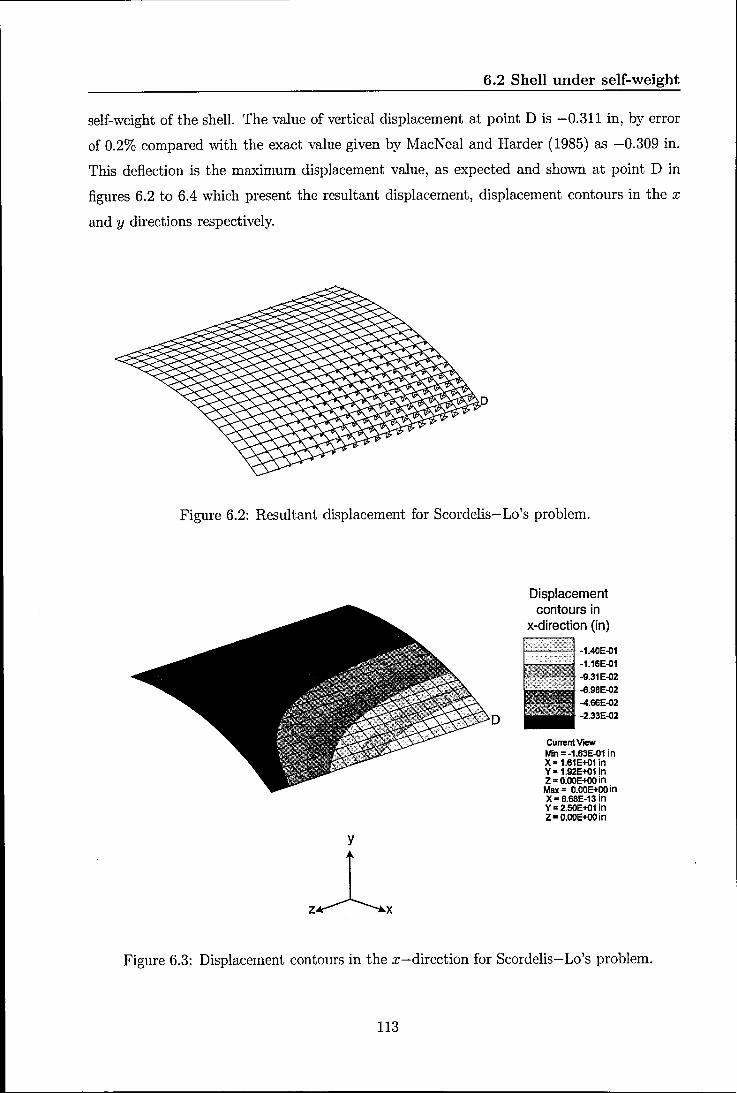
6.2 Shell under self-weight
self-weight of the shell. The value of vertical displacement at point D is -0.311 in, by error
of 0.2% compared with the exact value given by MacNeal and Harder (1985) as -0.309 in.
This deflection is the maximum displacement value, as expected and shown at point D in
figures 6.2 to 6.4 which present the resultant displacement, displacement contours in the x
and y directions respectively.
Figure 6.2: Resultant displacement for Scordelis-Lo's problem.
D
y
z~x
Displacement contours in
x-direction (in)
~----1- -1.40E'()1 -1.1GE'()1 -9.31E'()2 -6.9BE.02 -4.00E'()2 -2.33E'()2
Current VIeW Min = -1.63E'()1 in X· 1.G1E+C1 in Y· 1.92E+01 in Z = O.OOE+OO in Max = O.OOE+OO in X = G.68E-13 in Y = 2.50E+C1 in Z· O.OOE+OO in
Figure 6.3: Displacement contours in the x-direction for Scordelis-Lo's problem.
113

y
z~x
6.2 Shell under self-weight
Displacement contours in
y-direction (in)
I-'-~'-'+ -2.60E~1
'."-2.09E~1 Ilfr -1.5BE~1
·1.07E~1
-5.63E~
-5.3BE~
CunentVtI!NI Min = -3.11E~1 in X-1.61E+01 in Y = 1.92E+01 in Z = O.OOE+OO in Max = 4.55E~ in X = 6.6BE-13 in Y = 2.50E+01 in Z - O.OOE+OO in
Figure 6.4: Displacement contours in the y-direction for Scordelis-Lo's problem.
6.2.2 Hemicylindrical shell
The aim of this section is to compare the Nxx , Nyy and Nxy stresses by those obtained by
PfHiger (1957). Figures 6.5 (a) and (b) show the geometric, stratigraphic characteristics,
boundary conditions and finite element mesh of the whole domain for the considered prob
lem, where the radius R = 4 m, length L = 15 m, thickness t = 0.05 m, Young's modulus of
elasticity E = 3 X 10⁷ kPa and Poisson's ratio 1/ = O. This shell is loaded vertically by its
uniformly self-weight of 3.75 kJ.~/m2.
Under the self-weight of this shell, it moves downwards, as expected. The stresses Nxx , Nyy
and Nxy at element 314, as shown in figur~ 6.5 (b), are -30.10 kN/m2, -9.86 kN/m2 and
-14.57 kN/m2, respectively, with a small percentage error of 0.13%, 1.2% and 0.27%, respec
tively, compared with the analytical results -30.06 kN /m2, -9.74 kN /m2 and -14.61 kN /m2
,
respectively given by Pfliiger (1957).
114

6.3 Shell under external load
Uy=~
(a)
(b)
Figure 6.5: (a) The geometric, stratigraphic characteristics and boundary conditions, and
(b) finite element mesh for problem 6.2.2.
6.3 Shell under external load
6.3.1 Pinched cylindrical shell with rigid end diaphragm
The pinched cylinder has rigid end diaphragms and is subjected to a point load, as shown
in figure 6.6 (a). This is discussed in this section and the results are compared with the
results obtained by Sze et al. (2004). Due to the ability of shell elements to represent both
the inextensional bending actions and very complex membrane stress states (Liu and To,
1998), this example is another well-known benchmark problem (eg. Fliigge (1973), MacNeal
(1989), Kreja et al. (1997), Cho and Roh (2003) and Charmpis and Papadrakakis (2005)).
The geometrical and material properties are: R = 100 in, L = 200 in, t = 1 in, E = 30 X 103
psi, v = 0.3 and the point load is p = 12 X 103 lb (Sze et al., 2004). The boundary conditions
are, Ux = uy = Bz = 0 for arc AD, U X = By = Bz = 0 for side DC, uy = Bx = Bz = 0 for side
AB and Uz = Bx = By = 0 for arc BC, as shown in figure 6.6 (a).
Only one-eighth of the cylinder is considered due to symmetry, as shown in figure 6.6 (b),
with 20 x 20 elements. It is found that the deflection at the load point, i.e. at point C, is
115

6.3 Shell under external load
-86.82 in, by error of 4.28% compared with the numerical deflection -83.10 in obtained by
Sze et al. (2004).
rigid diaphragm (a)
z
rigid diaphragm
(b) force (p/4)
Boundary Conditions
arc AD: U =u =fl =0 x -)' z
side DC: u..: =~ =~ =0
side AB: u =fl=fl=O -)' x z
arc BC: u =fl=fl=O z x y
Figure 6.6: (a) Geometry and boundary conditions for the pinched cylindrical shell, and (b)
mesh for one-eighth of the cylinder.
6.3.2 Pullout of an open-ended cylindrical shell
The pullout of an open-ended cylindrical shell being pulled by a pair of radial forces, as
shown in figure 6.7, is modelled in this section and the result is compared with the result
obtained by Sze et al. (2004). The geometrical and material properties are: R = 4.953 in,
116

6.3 Shell under external load
L = 10.35 in, t = 0.094 in, E = 10.5 X 10⁶ psi, 1/ = 0.3125 and the point load is p = 40 X 103 lb.
Owing to symmetry, one-eighth of the shell is modelled, as in Section 6.3.1. The displacement
in the x-direction at point B is -4.613 in, by error of 1.34% compared with the numerical
result -4.551 in obtained by Sze et al. (2004).
free edge
Boundary Conditions
side DC: UX =~ =q =0
side AB: u =8.=8.=0 -)' x z
z arc BC: U =8.=8=0 z x y
free edge
Figure 6.7: Geometry and boundary conditions for the pullout of an open-ended cylindrical
shell.
6.3.3 Hemispherical shell with an 180 hole
The hemispherical shell subjected to alternating loads at the equator is a popular widely
used benchmark (e.g. MacNeal and Harder (1985), Stander et al. (1989), Simo et al. (1990),
Chroscielewsk et al. (1992), Sansour and Bufler (1992), Schieck et al. (1999), Zienkiewicz
and Taylor (2000) and Gruttmann and Wagner (2005)). This example is modelled and the
result is compared with this given by MacNeal and Harder (1985).
This problem is a very challenging example for several reasons. It is an excellent test of the
ability of an element to handle truly three-dimensional finite rotations. It is also useful in
checking the invariance of the elements to rigid body rotations and the sensitivity to mem
brane locking. Another feature which makes the problem challenging is that both membrane
and bending strains contribute significantly to the radial displacement at the loading point
(Zhu and Zacharia, 1996).
117

6.4 Conclusion
Figures 6.8 ( a) and (b) show the geometry of this hemispherical shell with a central hole of
18° in the top and side views respectively. The properties of this hemispherical shell are as
follows: radius R = 10 in, thickness t = 0.04 in, Young's modulus E = 6.825 X 10⁷ psi and
Poisson's ratio v = 0.3 under the action of two inward and two outward forces 90° apart. The
boundary conditions for this example are: free for nodes on the xy plane, uy = Ox = Oz = 0
for nodes on the xz plane and Ux = Oy = Oz = 0 for nodes on the yz plane.
o y
x
(a) (b)
Figure 6.8: The hemispherical shell (with 18° central hole) subjected to alternating IGads,
(a) top view and (b) side view.
By making use of the symmetry of the geometry, only one quadrant of the hemisphere is
analysed and each of the two alternating point loads on the quadrant is p = 1.0 lb. The
deflection at either one of the alternating load points is 0.097 in, by error of 0.03% compared
with the theoretical value 0.094 in given by MacNeal and Harder (1985).
6.4 Conclusion
To validate the implemented 4-noded quadrilateral shell element, the following five standard
widely-used benchmark shell problems have been modelled in this chapter using GeoFEAP2; .
• under self weight: Scordelis-Lo's roof and hemicylindrical shell,
• under external load: pinched cylindrical shell with rigid end diaphragm subjected to a
point load, pullout of an open-ended cylindrical shell being pulled by a pair of radial
118

6.4 Conclusion
forces, and hemispherical shell with an 18° hole subjected to alternating loads at the
equator.
It was found that the deflection in the vertical direction, displacement in the horizontal plane
perpendicular to the vertical direction, and Nxx , Nyy and N xy stresses compared well with
the analytical and/or numerical solutions given by MacNeal and Harder (1985), Sze et al.
(2004) and Pfliiger (1957).
119

CHAPTER 7
2D and 3D Study of Soil-Cooling
Tower-Interaction
7.1 Overview
Comparisons between the 2D and 3D applied load, and between 3D applied load and com
bined cooling tower-foundation-soil are then investigated and examined in this chapter. In
addition, the behaviour of the soil layer is investigated in the presence of temperature effect
at the shell and a change in the effect of soil shear strength, c, and soil angle of friction, cp.
7.2 Introduction
As shown in Chapter 2, the natural draught cooling towers are structures that are used to
reduce the temperature of the cooling-cycle water in thermal power plants. These towers are
large-scale civil engineering structures. The shell is the most important part of the cooling
tower, both in technical and financial terms (30% to 45% of the total cost) and also the
most sensitive, since its collapse would put all or part of the cooling tower out of action for
a considerable length of time. Hence, the shell is one of the fundamental factors influencing
the life of the cooling tower (Jullien et al., 1994).
A brief geometry of the shell of revolution, shown in figure 7.1, is now introduced as a base
for studying the geometry of the cooling tower shell. A plane curve, also called a meridian
and defined by angle (), rotates about an axis lying in the plane of the curve to produce a
surface of revolution. If this plane curve is a straight line, the shell is conical or cylindrical.
120

7.2 Introduction
The surface of revolution is also called the middle surface of the shell. Any point at this
surface can be described by first specifying the meridian on which it is located and secondly
by specifying a quantity, called a parallel circle and defined by angle rp, that varies along the
meridian and is constant on a circle around the axis of the shell (Jawad, 1994). z
axis of revolution
y
Figure 7.1: Coordinates, basic definitions and geometry of a surface of revolution.
Self-weight remains the most basic loading for cooling towers (Zingoni, 1999), where it is
controlled by two factors, the chosen material properties and high level structural system
(Liao and Lu, 1996). Hence, the tower considered for the analysis is a column-supported
hyperbolic cooling tower under dead load, 520 ft tall (158.5 m) earlier analysed by Gould
(1985) and later by other researchers (Aksu, 1996; Iyer and Rao, 1990; Karisiddappa et al.,
1998) for further studies. It should be noted that the height of this tower is in the range of
the tallest modern cooling towers which vary from around 60 m to in excess of 200 m (Busch
et al., 2002; Zingoni, 1999).
The geometry of the whole structure and soil, i.e. combined cooling tower-soil case, is
shown in figure 7.2. The variable thickness shell is supported by 36 pairs of columns where
these columns are circular in cross-section with a radius of 2.0 ft. The geometrical details
of the shell, columns, footing and soil used in the analysis are presented in Table 7.1 and
the thickness of the cooling tower shell is given in Table 7.2, where the acceleration due to
gravity, g, is taken as 32 ft/s2. It should be noted that the width and height of the soil are
121

7.2 Introduction
assumed to be 2 x (5 x rf) and 4 x rf, respectively (Potts and Zdravkovic, 2001).
Th.rQal __
GL
hs=370ft
5 C\I to
1025ft
zoom =4
I. 205ft 'I
1
1
Sbil I 1
1
1
1
1
circular footing
Figure 7.2: Geometric and stratigraphic characteristics for the combined cooling tower-soil
case.
122

7.2 Introduction
Table 7.1: Geometrical details for the hyperbolic cooling tower (Gould, 1985) and soil used
in the analysis.
Parameter description Parametric value
Shell
Height above throat level, ht 150 ft
Height below throat level, hs 370 ft
Radius at top, rt 125 ft
Radius at throat level, a 115ft
Radius at bottom, rs 200 ft
Thickness at top 1.33 ft
Thickness at throat level 0.75 ft
Thickness at bottom 4ft
Columns
Number of column pairs 36
Height of column 30 ft
Radius of column 2ft
Circular spacing of column pairs 10°
Footing
Height 10ft
Width 10ft
Soil
Height 825 ft
\Vidth 2050 ft
Table 7.2: Material properties used in the analysis (Gould (1985), Bowles (1988)).
Parameter Shell Column Footing Soil Unit
Young's modulus 0.576 x 10⁶ 0.72 X 10⁶ 0.72 X 10⁶ 0.3 X 10⁵ kipsjft2
Poisson's ratio 0.15 0.15 0.15 0.4
Weight density 0.15 0.15 0.15 0.004 kipsjft3
123

7.2 Introduction
Generally, as shown in figure 7.2, the meridional shape of the hyperboloid cooling tower, as
closed shell, consists of a lower and an upper hyperbola branches, which both meet at the
throat. Hence, it is efficient to choose the origin of the axes at this throat. The equation of
the generating curve in Cartesian coordinates becomes
(7.1)
where a is the radius at throat, z is the vertical coordinate along the axis of revolution and
b is a characterstic dimension of the shell that may evaluated as follows (Gould, 1985)
b = aht J(r; - a2 )
(7.2)
for the upper hyperboloid, Le. z > 0, and
b = ahs J(r; - a2 )
(7.3)
for the lower hyperboloid, i.e. z < O. In equations (7.2) and (7.3), rt and rB are the top and
base radius, respectively, and ht and hs are the vertical distances from the throat to the top
and to the base of the shell, respectively.
If R is the horizontal radius of the parallel circle then R2 = x2 + y2. Substituting R into
equation (7.1) results in
R2 Z2 ---=1 a2 b2
(7.4)
By defining the curvature parameter, kh as follows (Gould, 1977)
kt=J1+~: (7.5)
the meridian curve may be rewritten as follows:
(7.6)
The steps in this analysis are as follows:
1. Establishment of meridional geometry.
2. Selection of discretisation pattern, where the parts of this soil-cooling tower-interaction
project are modelled as follows:
(a) shell using the implemented 4-noded shell element, as introduced in Chapter 5,
124

7.3 2D and 3D cooling tower cases
(b) columns support using 3D 2-noded bar element (P. Gould, 2004; T. Hara, 2004),
(c) footing using first order 8-noded hexahedron element, and
(d) drained soil using 4-noded quadrilateral element in 2D, and first order 8-noded
hexahedron element in 3D, as introduced in Chapter 4.
3. Determination of the loading and its type. Self-weight and temperature loads are
considered in this analysis.
The following three cases are then investigated:
1. (a) Model the 3D shell and columns structure without the soil and foundation, but
with fixities representing the effect of the underlying soil and foundation.
(b) then using the z-reaction of (a) in the 3D applied load case.
2. 2D axisymmetric applied load.
3. 3D combined soil-structure interaction.
7.3 2D and 3D cooling tower cases
7.3.1 3D structure case
Figures 7.3 (a) and (b) show the 3D discretisation of the hyperboloidal shell and columns
support, for isometric and elevation views, respectively, where its geometric and stratigraphic
characteristics are shown in figure 7.2, comprising 998 nodes and 540 elements. The top view
of this mesh is shown in figure 7.4. In addition, Table 7.3 presents the thickness of the cooling
tower shelL The horizontal radius at every elevation is computed on using equations (7.1)
to (7.3). The base of every column is restrained in the x, y and z directions. The material
properties of the shell and columns are given in Table 7.2.
Every supporting column is a device for attaching the tower structure to the foundation.
Hence, these columns are very critical components of the cooling tower and their behaviour
is dominated by axial forces and motion (Yang and Kapania, 1983). It is therefore desirable
to use a sophisticated column element that contains axial displacements as degrees of free
dom.
125

7.3 2D and 3D cooling tower cases
The axial force resultant is computed by integration of the axial stress component over the
cross-sectional area of the member (Espinoza et al., 1995).
(a) (b)
§: Cl c: .~
a. I/)
C Q)
E Q)
ID 5
15
30
50
50
I/) I/) Q) c: ~ u oS ~ 1.33 1.25 1.00
0.75
0.75
1 ..... 1 \
H+++-+-+-I~~...feH'l--H+I------+--+O.75 )
50
50
11, \ 50
I1 \ \ 50
/ I 50
" I \ 50
I11 I / \ 50
/11 I \ \ \~ 20
WYVVVVVYY\f\f\ffJ1. 30
0.75
0.80
0.85
0.80
0.95
1.00
2.50
4.00
Figure 7.3: 3D discretisation for the hyperboloidal shell and columns support, (a) isometric
view and (b) elevation view.
After conducting the finite element analysis, it was found that this 3D shell-columns case,
as expected, is in static equilibrium under the self-weight, i.e.
2:1Vx = 2:Rx ~ 0 2:lVy = 2:Ry = 0 2: Wz = - 2: Rz = 4.0631 X 10⁵ kips
(7.7 a) (7.7 b) (7.7 c)
where W x, lVy and H'z are the weight of the structure in the x, y and z directions, re
spectively, and Rx, Ry and Rz are the reaction at supports in the x, y and z directions,
respectively. It should be noted that the 2: Wz value will be considered as the applied load
force in the next section.
126

7.3 2D and 3D cooling tower cases
200ft
! Figure 7.4: Top view for discretisation of the hyperboloidal shell and columns support.
Table 7.3: Thickness of the cooling tower shell (Gould, 1985).
Elevation from throat (ft) Shell thickness value (ft)
From To
+145 +150 1.33
+130 +145 1.25
+100 +130 1.00
+50 +100 0.75
0 +50 0.75
-50 0 0.75
-100 -50 0.80
-150 -100 0.85
-200 -150 0.90
-250 -200 0.95
-300 -250 1.00
-350 -300 2.50
-370 -350 4.00
127

7.3 2D and 3D cooling tower cases
Due to the self-weight of the cooling tower shell, stresses are produced on the wall. Figures 7.5
and 7.6 show the meridional and circumferential stresses resultant versus height, respectively,
at the 0° meridian, i.e. at the midpoint between the two adjacent supports. These stresses, as
expected, decrease as the height decreases from the bottom base. However, the meridional
stress decreases rapidly when -370 ft < z < -300 ft because the thickness of the shell
increases rapidly at this range from 1 ft to 4 ft. Figures 7.5 and 7.6 show good agrement
with the results obtained by Gould (1985) and Iyer and Rao (1990).
1 ! Zm
5~-----r----~r------r------r------r--~~
o ................................................................ : ............ :.: .. .
-5
·10 y--
·15
!I ~n; ·20 '0 :..c ·25
/1 :1-
-30 --- Gould (1985) I, If --t-- lyer and Appa Rso (1990) I[
--€- current -35 /' d -40 q ,
./.
""ioo -300 ·200 ·100 0 100 200 Height (11)
Figure 7.5: Meridional stress resultant versus height.
10r------r------~-----r------~-----r----~
o ................................................................ ! ...................... .
·10
·20
·50
·70 I I
·300
-.- Gould (1985) -+- Iyer and Appa Rso (1990) -e- current
·200 ·100 o 100 Height (11)
200
Figure 7.6: Circumferential stress resultant versus height.
128

7.3 2D and 3D cooling tower cases
7.3.2 3D applied load excluding temperature effect
Figures 7.7 and 7.8 show the side and details of top views for the 3D finite element mesh
of the applied load case, comprising 9504 nodes and 2304 elements, and an applied force of
4.0631 x 10⁵ kips, as shown in figure 7.8(c). It should be noted that this force is the same
as z-reaction from equation (7.7 c) in the 3D structure case, i.e. shell-columns case. The
drained soil is assumed to be an elasto-plastic material which obeys Drucker-Prager's model,
as introduced in Section 3.4.5, where c = 2 kips/ft2 and <P = 0° (Kerdi, 1974).
The boundary conditions for the mesh are as follows: the outer vertical boundary is restrained
in the x and y directions and is free to move in the z-direction. The base of the layer is
restrained in the x, y and z directions. For comparison purposes, it should be noted that the
axes have been taken, in this problem and the remaining 3D analysis, at the same position
as in figure 7.3.
reaction at support
4I·06~31XI~: ~@511 ',' -z=-40511 -10ft _~41Oft ~ 2@511 =1011
zoom = 17
J-y x
\c--t-----j-------oill 2@ 7.5ft 2@41 ft=820ft =1 5ft
1025ft S iI
z~40511 z=-41011
Figure 7.7: Side view of the 3D discretisation for the applied load case.
Figures 7.9 and 7.10 show the deviatoric stress and mean pressure, respectively, for the 3D
applied load at the AA-axis, as shown in figure 7.8(c), and z = -405 ft, -410 ft, -615 ft,
129

7.3 2D and 3D cooling tower cases
-820 ft and -1025 ft, respectively. In these figures, the vertical arrows refer to the position
of the applied load. Both deviatoric stress and mean pressure decrease as the absolute value
of z increases where the values are much greater at z = -405 ft and z = -410 ft, respectively.
In addition, the highest value of the deviatoric stress and mean pressure occur, as expected,
at node A, shown in figure 7.7, at level z = -405 ft. Moreover, the deviatoric stress and
mean pressure decrease, as expected, with the depth and away from the structure and they
tend to zero as x tends to the boundaries, i.e. away from the effect of the shell weight. More
attention is therefore given to the values at z = -405 ft and z = -410 ft in the remaining
study.
7.3.3 2D axisymmetric applied load excluding temperature effect
To compare the vertical settlement with the 3D applied load investigated in the last section,
a 2D axisymmetric applied load is investigated, where mesh is shown in the right hand side
of the central line in figure 7.7 is considered. The boundary conditions, shown in figure 7.11,
for the mesh are as follows: the outer vertical boundary is restrained in the x-direction and
is free to move in the y-direction. The base of the layer is restrained in the x and y directions.
Figure 7.11 shows the settlement contours in the y-direction for this problem. These con
tours decrease, as expected, with the depth and away from the load. However, these contours
are not symmetric around the load axis, as for the examples studied in Chapter 4, because
the central line has not been taken at the load axis.
Figures 7.12 (a) to (e) show the comparison of the vertical settlement [ft] for the 3D and
2D axisymmetric applied load at z = -405 ft, -410 ft, -615 ft, -820 ft and -1025 ft,
respectively. This settlement decreases, as expected, with the depth and away from the
structure, which tends to zero as x tends to the boundaries, i.e. away from the effect of the
shell weight. In addition, the maximum settlement at z = -405 ft and z = -410 ft occurs,
as expected, under the point load and then decreases as x tends to the central line. It is also
shown in these figures that there is a very big difference between the 2D and 3D analysis,
with maximum errors of about 78% and 76% at z = -405 ft and z = -410 ft, respectively,
although they undergo the same failure mechanism. This means that the analysis of the 3D
applied load case has to be considered with more attention to the settlement at z = -405 ft
and z = -410 ft levels.
130

(a)
----------
(c)
7.3 2D and 3D cooling tower cases
soil
(b)
circular strip footing
Figure 7.8: Top view for the 3D discretisation of the applied load case (a) finite element
.mesh, (b) title of the material types, and (c) geometry and load applied onto the footing,
represented by the vertical arrows.
131

7.3 2D and 3D cooling tower cases
3000,-----,--------.----f---'(C't'--I---,--------.--------,
2500
_ 2000
~ Cl.
~ Zl ~ 1500 .g ~ 5; o 1000
500
z-coordinate levels [ft]
-e- z=-405 -lE- z=-410 -+- z=-615 - z=-820 .- z=-1025 - - z=-1230
O~--~---~~~~~~HHjHr-~-~--~--~ -1500 -1000 -500 0 500 1000 1500
x[ft]
Figure 7.9: Deviatoric stress for the 3D applied load at the AA-axis, as shown in figure
7.8(c), and z = -405 ft, -410 ft, -615 ft, -820 ft and -1025 ft, respectively.
800
700
600
500 ;; ill Cl.
~ 400 I! :> III 1/1
I! 300 Cl. I: co .. ::!!
200
100
0
-100 -1500 -1000 -500
a:
o x 1ft)
500
z-coordinate levels [ft] -e- z--405 ""*" z=410 -t- z--615 -z--820 . - z=-1025 - . z=-1230
1000 1500
Figure 7.10: Mean pressure for the 3D applied load at the AA-axis, as shown in figure 7.8(c),
and z = -405 ft, -410 ft, -615 ft, -820 ft and -1025 ft, respectively.
132

7.4 3D combined soil-structure interaction
Total vertical displacement (ft)
1--'-'---'-4- -6.77E-m
~2!1~ -S.54E-m ~ -4.32E-m
-3.10E-m -1.87E-m -6.47E-OO
CunenlVteIW Min = -7.99E.Q2 ft x • 2.00E+02 ft Y • 8.30E+02 ft
Max= s.nE.Q3ft x .. 1.03E+03 ft Y • 8.20E+02 ft
Figure 7.11: Settlement contours in the y-direction for the 2D axisymmetric applied load.
7.4 3D combined soil-structure interaction
In this section, the full 3D cooling tower-foundation-soil model, as shown in figure 7.2, is
considered excluding the temperature effect, to compare with the 3D applied load case, and
including the temperature effect. T~e mesh of this model is a combination of the shell
columns mesh, as shown in figure 7.3, and foundation-soil, as shown in figure 7.7. The
boundary conditions is considered the same as explained in Section 7.3.2.
7.4.1 Excluding temperature effect
The aim of this section is to compare the deviatoric stress, mean pressure and settlement
at the AA-axis and z = -405 ft and/or -410 ft for the 3D applied load and soil-structure
interaction (SSI), excluding the temperature effect.
Figures 7.13 and 7.14 show the comparison of the deviatoric stress value for the 3D applied
load and combined SSI cases at the AA-axis and z = -405 ft and z = -410 ft, respectively,
excluding the temperature effect. Again, this value decreases with the depth and away from
the structure and it tends to zero as x tends to the boundaries and central line. In addition,
on comparing the maximum devlatoric stress value, it is found that there are errors of 36%
and 22% at z = -405 ft and z = -410 ft, respectively.
133

7.4 3D combined soil-structure interaction
(a) I~.---~----_r--~~----~----r----. g
.;; 'E .0.15 Q)
E ~ -4.2
~ '"
x (ft)
x (ft)
gO,02 c: .2 0 (3 Q) .= 3.02 "0
iii OD ... 'E Q)
> O.De Q)
;:; .;; 0 ...
"E ~ -4.1
Q)
E .0.12 Q)
'"
\ x (ft) d
x (ft) (e)
D.ODSr------.,.-----~----:.....:-----_,_----_r----___,
g c: o
-:;:. 0.Q05 o ~ '6 -4.01 .~
iii o 0.Q15 'E Q) > -11.02 Q)
.r= - .Q.025 .s E -0.03
I:~ -4.045 0 200
1~3DI .... 2D
400 600 800 1000 1200
x (ft)
Figure 7.12: Comparison of the vertical settlement (ft) for the 2D and 3D axisymmetric
applied load cases at z = (a) -405 ft, (b) -410 ft, (c) -615 ft, (d) -820 ft and (e) -1025
ft.
134

7.4 3D combined soil-structure interaction
3~r-----~------~------~-------r-------r------~
2500
z=.405ft -e- Applied load case -J!(- Combined SSI case
500
OL-----~----~~====~~~~==~~----~------~ -1500 -1000 500 1000 1500
Figure 7.13: Comparison of the deviatoric stress for the 3D applied load and combined SSI
cases at the AA-axis and z = -405 ft, excluding temperature effect.
Figure 7.15 shows the comparison of the mean pressure value for the 3D applied load and
combined SSI cases at the AA-axis and z = -405 ft, excluding the temperature effect.
Again, this value decreases with the depth and away from the structure and it tends to zero
as x tends to the boundaries and central line. Moreover, on comparing the ma.ximum mean
pressure value, it is found that there is an error of 27.6%.
Figures 7.16 and 7.17 show the comparison of the vertical settlement value for the 3D applied
load and combined SSI cases at the AA-axis and z = -405 ft and -410 ft, respectively,
excluding the temperature effect. Again, this value decreases with the depth and away from
the structure and it tends to zero as x tends to the boundaries. Furthermore, on comparing
the maximum settlement value, it is found that there are errors of 97.0% and 95.6% at
z = -405 ft and -410 ft, respectively, although they undergo a similar failure mechanism.
The results of this section show that there is a large error when comparing the deviatoric
stress, mean pressure and vertical settlement values between the 3D applied load and com
bined SSI cases. Hence, a 3D full model of the soil-cooling tower-interaction has to be
therefore considered.
135

7.4 3D combined soil-structure interaction
40
35
30
er ~ 25
~ :! 1l 20 .. U 00::: 0 z--410ft !! ii 15 c 1
-9- Applied load case 1 +- Combined SSI case
10
5
* 0 -1500 -1000 -500 0 500 1000 1500
x [ft)
Figure 7.14: Comparison of the deviatoric stress for the 3D applied load and combined SSI
cases at the AA-axis and z = -410 ft, excluding temperature effect.
BOO
700
600
500
~ a. ;& 400 I!! iil en I!! 300 a. 0:: to .. ~
200
100
0
-100 -1500 -1000 -500
Q
o x[ft]
za.405ft -9- Applied load case +- Combined SSI case
500 1000 1500
Figure 7.15: Comparison of the mean pressure for the 3D applied load and combined SSI
cases at the AA-axis and z = -405 ft, excluding temperature effect.
136

0.1
0.05
0
E: t -0.05
'6
3 :e -0.1
~ Cl
~ -0.15
i! .. E
-02 .. E " III
-0.25
-0.3
-0.35 -1500 -1000 -500
7.4 3D combined soil-structure interaction
o x[ft]
r-405ft -Er Applied load case ""*- Combined SSI case
500 1000 1500
Figure 7.16: Comparison of the settlement for the 3D applied load and combined SSI cases
at the AA-axis and z = -405 ft, excluding temperature effect.
0.1
0.05
0
E: c: i -0.05
'6 B :e -0.1
g! .. ~ -0.15
i! ~
-0.2 .. E r8
-0.25
-0.3
-0.35 -1500 -1000 -500 o
xIII] 500
z=..410ft -e- Applied load caSII -*- Combined SSI caSII
1000 1500
Figure 7.17: Comparison of the settlement for the 3D applied load and combined SSI cases
at the AA-axis and z = -410 ft, excluding temperature effect.
137

7.4 3D combined soil-structure interaction
7.4.2 Including temperature effect
In this section, deviatoric stresses and settlement are investigated with the effect of temper
ature on the cooling tower's shell, as introduced in Section 5.8. ~T is assumed as follows:
(7.7)
where t is the thickness of the shell, where its value at every elevation is defined in Table 7.3,
1In and Tex are the interior and exterior wall temperature of the cooling tower, respectively.
(71n - Tex ), or simply T considered in the remaining analysis, is equal to 45°e in winter
and 700 e in summer resulting from adding 25°e for sunshine (Meschke et al., 1991). The
coefficient of thermal expansion, fr, is assumed as 1O-5;oe in this analysis (Smith et al.,
1996).
Figures 7.18 and 7.19 show the comparison of the deviatoric stress for the 3D combined SSI
case when T = ooe, 45°e and 700 e at z = -405 ft and z = -410 ft, respectively. These
figures show that the maximum value of the deviatoric stress increases as T increases. This
is because the increasing of the stresses in the shell due to the temperature effect, especially
near the base of the tower as explained in Section 7.3.1. However, as expected, the increasing
of this maximum value at z = -405 ft is more clear compared to the increasing value at
z = -410 ft. In addition, from these figures, it is also noticed that the deviatoric stress value
decreases, as expected, with the depth and away from the structure and it tends to zero as
x tends to the boundaries and to the central line.
Figures 7.20 and 7.21 show the comparison of the settlement for the 3D combined SSI case
when T = ooe, 45°e and 700 e at z = -405 ft and z = -410 ft, respectively. These figures
show that the settlement increases as the temperature value increases. This is because the
increasing of the deviatoric stress value due to the increasing of the temperature value, as
explained in the previous paragraph. The behaviour of the soil layer is similar for different
temperatures at the same vertical level, experiencing the failure mechanism explained in
Section 4.3.2. However, temperature does not have a major effect on the deviatoric stress of
the soil, but does affect the cooling tower shell.
138

7.4 3D combined soil-structure interaction
2~r-------r-------r---~--r--T----~------~----~ ! ....
1800
1600
1400
l: 1200 a :I ~1~ .g
I 800
600
400
200
I
_1~L------_1-4l001-0-----_-5ood==::2...."IiH!~==500~-----100-0-0 -------.J1500
Figure 7.18: Comparison of the deviatoric stress for the 3D combined SSI case when T =
O°C, 45°C and 70°C at z = -405 ft.
35
30
25
'" ~20 .. .. ,g: .. ~ 15 .~ c
10
5
0 -1500 -1000 -500 o
x[ft) 500
z=.<410 ft
-e- T"cfc + T-4S'C
- T"7cfc
1000 1500
Figure 7.19: Comparison of the deviatoric stress for the 3D combined SSI case when T =
O°C, 45°C and 70°C at z = -410 ft.
139

7.4 3D combined soil-structure interaction
0.12
0.1
0.08
s: 0.06
t '6 0.04
11 :e ..
0.02 > .. £; .s ;: 0 .. E ., ii -0.02 (I)
-0.04
-0.06
-0.08 -1500 -1000 -500 1000 1500
Figure 7.20: Comparison of the settlement for the 3D combined SSI case when T = O°C,
45°C and 70°C at z = -405 ft.
0.12
0.1
0.08
s: c 0 0.06
I '" ~ 0.04 ., > .. £; 0.02 .s ;: ., E
0 ., l3 r'l
-0.02
-0.04
-0.06 -1500 -1000 -500 1000 1500
Figure 7.21: Comparison of the settlement for the 3D combined SSI case when T = O°C,
45°C and 70°C at z = -410 ft.
140

-------------------------------------- ---
7.5 Parametric study of the 3D cooling tower
7.5 Parametric study of the 3D cooling tower
7.5.1 Effect of soil shear strength (c)
Figures 7.22, 7.23 and 7.24 show the comparison of the deviatoric stress for the 3D SSI
and T = O°C, 45°C and 70°C at z = -410 ft for c = 0.2 kipsjft2, i.e. for very soft clay,
c = 2 kipsjft2, i.e. for hard clay, and c = 13 kipsjft2, i.e. for very hard clay, respectively,
where rp = 0° (Kerdi, 1974). In these figures, it is shown that the maximum value of the
deviatoric stress increases slightly as the temperature increases at the same value of c, and
also increases as c increases at the same value of temperature. It is also noticed that the
deviatoric stress decreases away from the structure and it tends to zero when the absolute
value of x increases away from the effect of the shell weight. In addition, the deviatoric
stress decreases as the absolute value of x decreases from the point load to the central line.
Furthermore, this stress increases at the central line as c increases. This is because the
increasing of c makes the soil more resisting of transferring the stress from the point load.
35r---~----.---~--~r_--_.---,
30
10
5
_1~~----:-'1000~==='a,-5~OO====~~O ~.!!!==:::::I50::='O A>===10olll00'-----.-J1500
xIII]
Figure 7.22: Comparison of the deviatoric stress for the 3D combined SSI case when T =
O°C, 45°C and 70°C at z = -410 ft, where c = 0.2 kipsjft2.
141

7.5 Parametric study of the 3D cooling tower
35
30
25
~ Cl. ~20
i .. ~ 15 .m ~
10
5
0 -1500
III
-1000 -500 o x[ft)
b
500
c=2k1~
-e- T=cf'C:1 -+- T-4s"C - T=7cf'C
1000 1500
Figure 7.23: Comparison of the deviatoric stress for the 3D combined SSI case when T =
O°C, 45°C and 70°C at z = -410 ft, where c = 2 kipsjft2.
~r------.-------.------~-------r-------r------,
40
35
130
.. 25
I ~ 20
.! c 15
10
.... Q
C=13kq,sm2
-e- T=cf'C -+- T=4s"C - T=7cf'C
· J OL-____ ~ ______ ~ ______ ~ ______ _L ______ _L ______ ~
-1500 -1000 -500 0 500 1000 1500 x[ft)
Figure 7.24: Comparison of the deviatoric stress for the 3D combined SSI case when T =
O°C, 45°C and 70°C at z = -410 ft, where c = 13 kipsjft2.
142

7.5 Parametric study of the 3D cooling tower
7.5.2 Effect of soil angle of friction (cjJ)
Figures 7.25, 7.26 and 7.27 show the comparison of the deviatoric stress for the 3D SSI
and T = O°C, 45°C and 70°C at z = -410 ft for cp = 00, 100 and 200, respectively, where
c = 2 kipsjfe. In these figures, it is shown that the maximum value of the deviatoric stress
increases slightly as the temperature increases for the same value of cp, and also increases
slightly as cp increases for the same value of temperature. It is also noticed that the deviatoric
stress decreases as the absolute value of x increases away from the effect of the shell weight,
and also decreases as the absolute value of x decreases from the point load to the central
line.
35
30
25
~
120 III ~ .. • 11 .9 15 .~ c!l
10
5
0 -1500 -1000 -500 o
x [ft] 500
1
-& T=O"C :1 ""*- T~s"C - T=70"C
1000 1500
Figure 7.25: Comparison of the deviatoric stress for the 3D combined SSI case when T =
O°C, 45°C and 70°C at z = -410 ft, where cp = 00.
143

7.5 Parametric study of the 3D cooling tower
~r------.-------'-------;-------'-------'------~
30
25
10
5
_1~L:------:_1-:-oooL-------5..JOO':--------IO-------500-1-------1....LOO-0-------.J1500 x[ft]
Figure 7.26: Comparison of the deviatoric stress for the 3D combined SSI case when T =
O°C, 45°C and 70°C at z = -410 ft, where cP = 10°.
~.------.------.-------~r------'-------r----~
30
25
10
5
-500
OL_ ____ ~L_ ____ ~L_ ____ ':_L_ ______ L_ ______ L_ ____ __l
-1500 -1000 1500 o x[ft]
500 1000
Figure 7.27: Comparison of the deviatoric stress for the 3D combined SSI case when T =
O°C, 45°C and 70°C at z = -410 ft, where cP = 20°.
144

7.6 Conclusion
7.6 Conclusion
Self-weight and temperature remain the most important basic loading for cooling towers.
Hence, columns-supported hyperbolic cooling tower under dead load, which has dimensions
in the range of the tallest modern cooling towers, has been modelled. It was found that
this 3D shell-columns case, as expected, is in static equilibrium under the self-weight. Due
to the this load, stresses are produced at the shell wall, where the meridional and circum
ferential stresses decrease, as expected, as the height of the cooling tower decreases from
the bottom base. However, the meridional stress decreases rapidly at the bottom i th of
the cooling tower height because the thickness of the shell increases rapidly at this range
until it becomes the same radius of the column for achieving the stability of the structure.
Furthermore, these stresses were in good agrement and compared well with the numerical
solutions obtained by other authors. Comparisons have been made between the 2D and 3D
applied load, 3D applied load and combined soil-cooling tower-interaction, and 3D combined
soil-cooling tower-interaction excluding and including the temperature effect upon the cool
ing tower shell.
In the 3D applied load analysis, it was found that the deviatoric stress and mean pressure
values decrease as the soil depth increases where these values are much greater at the ground
and SSI levels. In addition, the highest value of the deviatoric stress and mean pressure oc
cur, as expected, at the middle of the ground level. Moreover, the deviatoric stress and mean
pressure values decrease, as expected, with the depth and away from the structure and they
tend to zero as the horizontal distance tends to the boundaries, i.e. away from the structure
effect. More attention was therefore given to the results at ground and final SSI levels in the
remaining study.
In the 2D a.xisymmetric applied load analysis, the settlement contours decrease, as expected,
with the depth and away from the load and they tend to zero as the horizontal distance tends
to the boundaries, i.e. away from the structure effect. However, these contours are not sym
metric around the load axis, because the central line has not been taken at the load axis.
In addition, the maximum settlement at ground and final SSI levels occurs, as expected,
under the point load and then decreases as the horizontal distance tenus to the central line.
Furthermore, it was also found that there is a very big difference between the 2D and 3D
applied load analysis, with maximum errors at ground and final SSI levels, although they
undergo the same failure mechanism. This means that the analysis of the 3D applied load
145

7.6 Conclusion
case has to be considered when compared with the 2D axisymmetric applied load case.
The 3D soil-cooling tower-interaction excluding and including the temperature effect have
been investigated and compared with the 3D applied load, where more attention has been
given to ground and final SSI levels. On comparing the deviatoric stress, mean pressure
and vertical settlement values for 3D applied load and SSI excluding the temperature effect,
it was found that these values decrease with the depth and away from the structure and
they tends to zero as the horizontal distance tends to the boundaries and central line. In
addition, comparing between these two cases for maximum deviatoric stress, mean pressure
and vertical settlement have indicated that there are large errors at ground and final SSI
levels. This means that, the 3D full model of the soil-cooling tower-interaction has to be
therefore considered when compared with the 3D applied load case.
When including the temperature effect, it was found that the deviatoric stress value de
creases, as expected, with depth and away from the structure and it tends to zero as the
horizontal distance tends to the boundaries and to the central line. Due to increasing of
the stresses at the cooling tower shell in presence of the temperature effect, the maximum
value of the deviatoric stress increases as the temperature increases, and therefore the ver
tical settlement increases as the temperature value increases as well. It should be noted
that the incr:easing of the maximum value of the deviatoric stress and vertical settlement at
the ground level is more clear compared to their increasing at the final SSI level. However,
temperature does not have a major effect on the deviatoric stress of the soil, but does affect
the cooling tower shell as explained in Chapter 2.
The behaviour of the soil layer for the 3D soil-cooling tower-interaction has been investi
gated with the effect of the soil shear strength, c, and soil angle of friction tjJ. The effect
of c indicated that the deviatoric stress decreases, as expected, away from the structure
and it tends to zero when the absolute of the horizontal distance increases away from the
structure effect. In addition, the maximum value of the deviatoric stress increases slightly
as the temperature increases at the same value of c, and also increases as c increases at the
~ame value of temperature. Moreover, the deviatoric stress decreases as the absolute value
of the horizontal distance decreases from the point load to the central line. Furthermore,
this stress increases at the central line as c increases. This is because the increasing of c
indicates an increase in the shear strength of soil.
146

7.6 Conclusion
The effect of IjJ indicated that the maximum value of the deviatoric stress increases slightly as
the temperature increases for the same value of 1jJ, and also increases slightly as IjJ increases
for the same value of temperature. It was also noticed that the deviatoric stress decreases
as the absolute value of the horizontal distance increases away from the structure effect, and
also decreases as the absolute value of the horizontal distance decreases from the point load
to the central line. The designer needs therefore to ensure that enough modelling of soil
conditions is done and an extensive site investigation is required to ensure that the variation
in soil properties is represented correctly.
147

CHAPTER 8
Effect of Different Designs for Cooling
Tower
8.1 Overview
The soil behaviour for the same cooling tower shell studied in Chapter 7 for different types
of footings, circular and pads, affected by different types of columns is investigated in this
chapter. Vertical and horizontal soil layers are also considered.
8.2 Introduction
The same hyperbolic cooling tower shell, that has been investigated in Chapter 7, is consid
ered for further study in this chapter. The same geometrical details for the shell and soil,
and material properties, introduced in Tables 7.1 and 7.2 respectively, are considered as well.
The 3D combined soil-structure, v.ith different types of footings and columns, are investi
gated in Sections 8.3 and 8.4. However, different geometric, stratigraphic characteristics and
mesh, are used and described in the next paragraphs.
Figures 7.2 and 8.1 show the geometric and stratigraphic characteristics for the cooling tower
shell, two columns attached to circular and pad footings respectively, and soil. In addition,
figures 8.2 and 8.3' (a), (b) and (c) show the top, isometric and elevation views, respectively,
for the cooling tower shell, circular footing with two columns and one column, respectively.
148

8.2 Introduction
Figures 8.4 (a), (b) and (c) show the top, isometric and elevation views, respectively, for the
cooling tower shell, and two columns attached to pad footings. Moreover, figure 8.5 shows
the design and construction of two typical natural draught cooling towers with one column
attached to pad footings. Furthermore, figures 8.6 (a), (b) and ( c) show the top, isometric
and elevation views, respectively, for the cooling tower shell, pad footings and two columns,
one column, respectively.
It should be noted that the thickness of the cooling tower shell being studied here is shown
in figure 7.3 and further listed in Table 7.3. In addition, the origin of the axes are assumed
at the throat as explained in Chapter 7.
The same steps used in Chapter 7 will be applied here, i.e.
1. (a) Model the 3D shell and columns structure without the soil and foundation, but
with fixities representing the effect of the underlying soil and foundation.
(b) then using the z-reaction of (a) in the 3D applied load case.
2. 2D axisymmetric applied load.
3. 3D combined soil-structure interaction.
These steps are repeated for the most commonly used arrangements in practice (Gould, 1985;
Wittek and Kratzig, 1996)
1. one column attached to circular footing.
2. two columns attached to pad footings.
3. one column attached to pad footings.
It is found that the 3D full model of the cooling tower, with different types of columns and
footings, and soil has to be considered and compared with the 3D applied load case which
has to be assumed and compared with the 2D axisymmetric applied load. It should be noted
that results in the next few sections are taken at the central line in the case of one column
and with an angle of 5°, i.e. along the AA axis as shown in figure 7.8, for the case of two
columns.
149

h,=150ft
Thmal __
h.=370ft
GL
1025ft
zoom =4
11 205ft 'I
1
1
Sbil I 1
1 1
1
1
8.2 Introduction
Figure 8.1: Geometric and stratigraphic characteristics for the cooling tower shell, two
columns, pad footings and soil case.
150

8.2 Introduction
(a) (b)
'/1
I \ \
h /1 \ \ \\ \ ~
ij / /1 / \ \ \ \~ /I / I \ \
IY ;1/\/\/\/\/\/\/\/\/\/\/\]\ ~
(c)
Figure 8.2: 3D discretisation for the cooling tower shell, two columns and circular footing
where (a) top view, (b) isometric view and (c) elevation view.
151
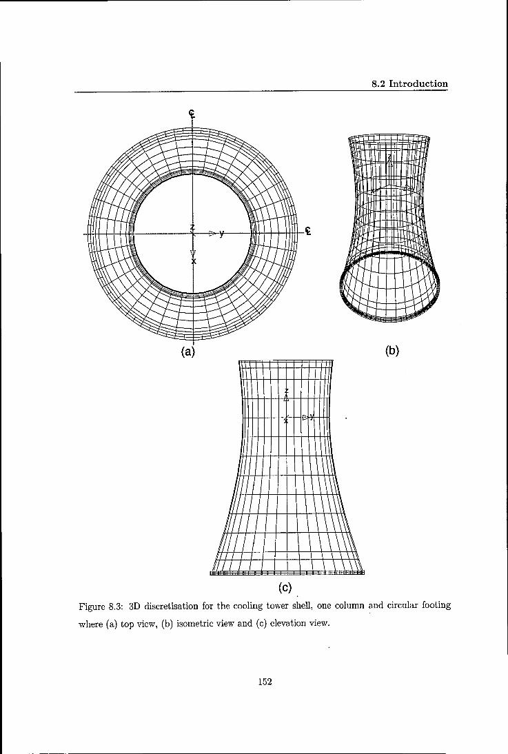
8.2 Introduction
(a) (b)
1/1 \ \ 11/ \ 1\'
1,1/ I I \ \ \ \\\ Ill/I \ \ \\\ PI/I \ \ \ \~ 'I I I I I \ \ \ \ \~
51 / / / I \ \ \ \ \\
(c)
Figure 8.3: 3D discretisation for the cooling tower shell, one column and circular footing
where (a) top view, (b) isometric view and (c) elevation view.
152

8.2 Introduction
(a) (b)
(c)
Figure 8.4: 3D discretisation for the cooling tower shell, two columns and pad footings where
(a) top view, (b) isometric view and (c) elevation view.
153

8.2 Introduction
(a)
(b)
Figure 8.5: Typical natural draught cooling tower in Trino Vercellese, Italy (a) design and
construction of two towers, and (b) one column attached to pad footings (Bierrum, 2005).
154

8.2 Introduction
(a) (b)
(c) Figure 8.6: 3D discretisation for the cooling tower shell, one column and pad footings where
(a) top view, (b) isometric view and (c) elevation view.
155

8.3 Type of footings
8.3 Type of footings
8.3.1 Circular footing
In this section, the behaviour of soil is investigated for the case of circular footing attached
to two columns and one column, as shown in figures 8.2 and 8.3, respectively.
Figures 8.7 (a), (b) and (c) and 8.8 (a), (b) and (c) show the comparison of the deviatoric
stress at z = -405 ft and z = -410 ft, respectively, for the case of circular footing with
affected to one column and two columns for (a) T = ooe, (b) T = 45°e and (c) T = 70oe. As shown in these figures, the deviatoric stress decreases with the depth and away from
the structure and it tends to zero when the absolute value of x increases away from the
effect of the shell weight. In addition, the deviatoric stress decreases as the absolute value
of x decreases from the point load to the central line. Moreover, it is also noticed that the
deviatoric stress in the case of one column is slightly higher than the deviatoric stress in the
case of two columns for different temperature values. This is because in the two columns
case, the sum of this stress in the x and y directions is equal to zero, as in equations (7.7
a, b) so the stress in the z-direction is only distributed to the foundation and then to the
soil. However, total deviatoric stress is transferred to the soil via the foundation. In ad
dition, this difference increases as the temperature value and the absolute value of x increases.
Figures 8.9 (a), (b) and (c) and 8.10 (a), Cb) and (c) show the comparison of the vertical
settlement at z = -405 ft and z = -410 ft, respectively, for the case of circular footing with
one column and two columns for (a) T = ooe, (b) T = 45°e and (c) T = 70oe. These figures
show that the maximum settlement, which occurs at the point load, in the one column case is
higher than the maximum settlement in the two columns case at z = -405 ft and z = -410
ft. This is expected because the deviatoric stress in the one column case is higher than the
maximum settlement in the two columns case. In addition, the settlement value decreases
away from the structure to the boundaries and to the central line. Furthermore, this value
tends to zero as x tends to the boundaries.
Discussion in this section indicates that the deviatoric stress and settlement in the two
columns case are smaller than those in the one column case, where the foundation is designed
as a circular footing. Hence, from a design point of view, it is recommended that the two
columns are better than the one column.
156
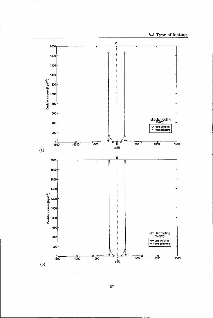
8.3 Type of footings
~ 2000
~ (
1800
1600
1400
;;-s'1200 ~ ell ell
~ 1000 .g ~ 800 ] c
600
circular footing 400 T=cfc
1-& one column I1 -*- two columns
200
0 ;\. ..I
-1500 -1000 -500 0 500 1000 1500
(a) x [ftl
~ 2000
1800
1600
1400
~ s'1200 ~ ell
'" ~ 1000
~ ca 800 .~
c 600
circular footing 400 T=4s"C
1-& one column 1 I -*- two columns
200
0 ~ J
-1500 -1000 .. 500 0 500 1000 1500
(b) x [ftl
157

(c)
8.3 Type of footings
2&Wr-------,_------_r------~~r_------,_------_r------~
2000
~ 11500 ~
I J ca 1000 ~ c
Q
circular footing T=7o"C
-e- one column *" two columns
oL-----~~--~~====~~~~====~~----~----~ -1500 -1000 -500 o
x [ftl 500 1000 1500
Figure 8.7: Comparison of the deviatoric stress at z = -405 ft in the case of circular footing with one column and two columns for (a) T = O°C, (b) T = 45°C and (c) T = 70°C.
158

8.3 Type of footings
35 ~
30
25
~ ill ~20 '" '" ]l '" ~ 15 .~ GI C
10
circular footing T=cfc
5 I-e- one column 11
~l-L: -+- two columns
tr *"-If-*' -p 0
-1500 -1000 -500 0 500 1000 1500
(a) x [ft)
~ 35
30
25 , ~20 = ]l '" .!.l 5 15 :m > GI C
10
circular footing T=45"C
5 I-e- one column .1 -+- two columns
~ 0 ~ i -p
-1500 -1000 -500 0 500 1000 1500
(b) x [ft)
159

(c)
35
30
25
10
5
o -1500
~ -1000 -500
:
:
: :
: :
: :
~ o
X [It] 500
8.3 Type of footings
circular footing T=7o"C
I-e- one column 1 -*- two columns
--=p 1000 1500
Figure 8.8: Comparison of the deviatoric stress at z = -410 ft in the case of circular footing with one column and two columns for (a) T = O°C, (b) T = 45°C and (c) T = 70°C.
160

161

0.15
0.1
[[ 0.05 c
i .., ~
0
~ CD :5 .5 -0.05 C CD E Gl i3 Gl -0.1 If)
-0.15
-0.2 -1500
(c) -1000 -500 o
x [ft] SOD
8.3 Type of footings
circular footing T=7o"C
-9- one column -*- two columns
1000 1500
Figure 8.9: Comparison of the vertical settlement [ft] at z = -405 ft in the case of circular footing with one column and two columns for (a) T = O°C, (b) T = 45°C and (c) T = 70°C.
162

163

(c)
8.3 Type of footings
et o.1.-----"""T"""----.-------T-----.------.--------.
0.05
.5 C -0.05
i ., Cl)
-0.1 circular footing
T=7rfC
-e- one column -)j(- two columns
-O.15L-----L----L----~0L-----L---~L----~ -1500 -1000 -500 500 1000 1500
x 1ft]
Figure 8.10: Comparison of the vertical settlement [ft] at z = -410 ft in the case of circular footing with one column and two columns for (a) T = O°C, (b) T = 45°C and (c) T = 70°C.
164

8.3 Type of footings
8.3.2 Pad footings
In the current section, the behaviour of soil is investigated in the case of pad footings at
tached to two columns and one column, as shown in figures 8.4 and 8.6, respectively.
Figures 8.11 (a), (b) and (c) and 8.12 (a), (b) and (c) show the comparison of the deviatoric
stress at z = -405 ft and z = -410 ft, respectively, for the case of pad footings attached to
one column and two columns for (a) T = O°C, (b) T = 45°C and (c) T = 70°C. As shown
in these figures, the deviatoric stress decreases with the depth and away from the structure
and it tends to zero when the absolute value of x increases away from the effect of the shell
weight. In addition, the deviatoric stress decreases as the absolute value of x decreases
from the point load to the central line. Moreover, the deviatoric stress at z = -405 ft and
z = -410 ft in the case of one column is slightly higher than the deviatoric stress in the
case of two columns for different temperature values. This is because in the two columns
case, the sum of this stress in the x and y directions is equal to zero, as in equations 7.7
a,b,c so the stress in the z-direction is only distributed to the foundation and then to the
soil. However, the total deviatoric stress is transferred to the soil via the foundation, i.e. for
the same reason explained in the previous section. Furthermore, this difference increases at
z = -405 ft and decreases at z = -410 ft as the temperature value increases.
Figures 8.13 (a), (b) and (c) and 8.14 (a), (b) and (c) show the comparison of the vertical
settlement at z = -405 ft and z = -410 ft, respectively, for the case of pad footings at
tached to one column and two columns for (a) T = O°C, (b) T = 45°C and (c) T = 70°C.
These figures show that the maximum settlement, which occurs at the point load, in the one
column case is higher than the maximum settlement in the two columns case at z = -405
ft and z = -410 ft. This is expected because the deviatoric stress in the one column case is
higher than the maximum settlement in the two columns case. In addition, the settlement
value decreases away from the structure to the boundaries and to the central line.
Discussion in this section indicates that the deviatoric stress and settlement in the two
columns case are smaller than those in the one column case, where the foundation is designed
as pad footings. Hence, from a design point of view, it is again recommended that the two
columns is better than the one column.
165

8.3 Type of footings
~ 4000
3500
3000
~ ~ 2500 tn tn
~ ut .g 2000
~ .s: 11)
0 1500
1000 pad foolings T=cfc
500 1-& one column 1 -+ two columns
0 ~ ,;, ,,/ -1500 -1000 -500 0 500 1000 1500
(a) x [ft)
~ 4500
(
4000
3500
~ 3000 c. ~ ut ut 2500 ~ ut .2
I 2000 11)
0
1500
1000 pad foolings
T=4SOC
500 1-& one column 1
--)j!- two columns
0 ~ ~-b
-1500 -1000 --500 0 500 1000 1500
(b) x [ft)
166

8.3 Type of footings
~ 5000
4500
4000
3500 ~ iil
~ 3000 III III ,g:
2500 III
.g 0 ;;; 'S: 2000 Cl> Cl
1500
1000 pad foolings
T=7cfc Iv one column I -+- two columns
500
0 ~ .);
-1500 -1000 -500 0 500 1000 1500
(c) x [ftJ
Figure 8.11: Comparison of the deviatoric stress at z = -405 ft in the case of pad footings with one column and two columns for (a) T = O°C, (b) T = 45°C and (c) T = 70°C.
167

8.3 Type of footings
C&-35
30
25
",-
~ ~20 1/1 1/1
~ 1/1
.s.!
.9 15 ca '> QI Cl
10 pad footings
T=cfc
5 1-& one column .1 -+- two columns
$-
"'~ &,-0
-1500 -1000 -500 0 500 1000 1500
(a) x [It)
C&-35
L
30
25
'" a. ~20 1/1 1/1
~ .s.! .9 15 ca '> QI Cl
10 pad foolings
T=4SOC
5 1-& one column I _.J!<- two columns
~ er-0
-1500 -1000 -500 0 500 1000 1500
(b) x [It)
168

8.3 Type of footings
~r-------~------~--~~-~T-~r---~------~------~
30
25
10
5
(c)
Figure 8.12: Comparison of the deviatoric stress at z = -410 ft in the case of pad footings with one column and two columns for (a) T = O°C, (b) T = 45°C and (c) T = 70°C.
169

8.3 Type of footings
~ 0.15
0.1
E: 0.05 c 0
~ :c ij 0 '2 Q) > Q)
oS .5 -0.05 c: Q)
E Q)
E Q) -0.1 IIJ
pad footings T=o"C
-Er one column -0.15 -+- two columns
-0.2 -1500 -1000 -500 0 500 1000 1500
(a) x [ft]
~ 0.15
0.1
E: 0.05 c 0
'fl ~ .., ~
0
~
~ .5 -0.05 c: Q)
E ~ Q) -0.1 IIJ
padfootings T=45'lC
-Er one column -0.15 -+- two columns
-0.2 -1500 -1000 -500 0 500 1000 1500
(b) x [ft]
170

0.15
0.1
§: 0.05 c
i 'i3 1j 0 :e Q) >
~ .5 ..Q.05 C Q)
E Q)
E Q) ..Q.1 Cl)
..Q.15
-0.2 ~1500
(c) -1000 -500 o
x[ft) 500
8.3 Type of footings
pad footings T=7r:fC
-e- one column ""*" two columns
1000 1500
Figure 8.13: Comparison of the vertical settlement [ft] at z = -405 ft in the case of pad footings with one column and two columns for (a) T = O°C, (b) T = 45°C and (c) T = 70°C.
171

8.3 Type of footings
~ 0.15.-----,-----.------T----.-------,r------,
0.1
!5: c
~ I!! '5 0.05
~ Cl) > Cl)
;; .5 - 0 c Cl)
E Cl)
E Cl) IJ)
pad footings
-0.05 T=cfc -B- one column -lIE- two columns
-0.1 -1500 -1000 -500 0 SOD 1000 1500
(a) x [It)
~ 0.15
0.1
!5: c 0
'B I!! '5 0.05 1j ;: Cl) > Cl) ;; .5 i: 0 Cl)
E Cl)
E Cl) IJ)
pad footings -0.05 T=4sOC
-B- one column -lIE- two columns
-0.1 -1500 -1000 -500 0 500 1000 1500
(b) x [ft)
172

8.3 Type of footings
~ 0.15r------;------,r-----r------,-----.-----,
Figure 8.14: Comparison of the vertical settlement [ft] at z = -410 ft in the case of pad footings with one column and two columns for (a) T = O°C, (b) T = 45°C and (c) T = 70°C.
173

8.4 Type of columns
8.4 Type of columns
B.4.1 One column
The behaviour of soil for the case of one column sitting on circular and pad footings, as
shown in figures 8.3 and 8.6, respectively, is studied.
Figures 8.15 (a), (b) and (c) and 8.16 (a), (b) and (c) show the comparison of the deviatoric
stress at z = -405 ft and z = -410 ft, respectively, for the case of one column sitting on
circular and pad footings for (a) T = O°C, (b) T = 45°C and (c) T = 70°C. As noticed in
these figures, the deviatoric stress decreases with the depth and away from the structure
and it tends to zero when the absolute value of x increases away from the effect of the shell
weight. In addition, figures 8.15 and 8.16 show that the maximum deviatoric stress in the
case of pad footings is much higher than the deviatoric stress in the case of circular footing
for different temperature values at z = -405 ft. Moreover, this difference increases as the
temperature value increases. The big difference between the circular and pad footings cases
is because the circular footing spreads the stress over a big area under the columns rather
than the pad footings. However, the deviatoric stress at z = -410 ft in the case of pad foot
ings is slightly smaller than the deviatoric stress in the case of circular footing for different
temperature values.
In the one column case, it is noticed that the deviatoric stress and settlement in the circular
footing case are smaller than those in the pad footings case. Hence, from a design point of
view, it is recommended that the circular footing is better than the pad footings.
174
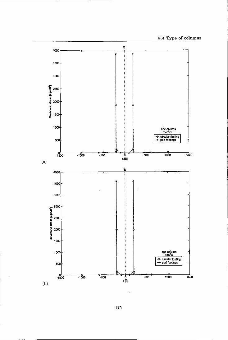
8.4 Type of columns
et. 4000
3500
3000
~ 2500
~ j 2000 .. 1 "50
011 1500 c
1000 one column T=cfc
500 1-& circular footing 1
-l/:- pad footlngs
0 ~ .i. ./
-1500 -1000 -500 0 500 1000 1500
(a) x [It]
et. 4500
4000
3500
_ 3000
~ Co :i! ;; 2500 .. i .g 2000 .9 ] c
1500
1000 one column T=45°C
500 1-& circular footing 1 *" pad footlngs
0 "'- ..). -1500 -1000 -500 0 500 1000 1500
(b) x [It]
175

(c)
8.4 Type of columns
~ 4&ror_-------r--------r-------~--------r--------r------~
4000
3500
_ 3000
~ .9-~ 2&ro
i .g 2000 S .~ c 1500
1000
500
* i
one column T=7rfC
1
-0- circular footing I -4- pad foolings
~ j" oL-----~~----_.~-===~~~~===-~~----~------~
-1&ro -1000 -500 0 500 1000 1500 x [ftl
Figure 8.15: Comparison of the deviatoric stress at z = -405 ft in the case of one column attached to circular and pad footings for (a) T = O°C, (b) T = 45°C and (c) T = 70°C.
176

8.4 Type of columns
~ 35
30
25
~ a. ~ 20
= 1: on
i 15 '~ c one column
T=cfc 10 -Er circular footing
*- pad footings
5
0 -1500 -1000 -500 0 500 1000 1500
(a) x [ft]
~ 35
30
25
~ a. ~20
= 1: on ,So!
~ 15 '50
011 C
one column 10 T=45"C
-Er circular footing *- pad footings
5
0 -1500 -1000 -500 0 500 1000 1500
(b) x [ft]
177

(c)
8.4 Type of columns
~r-------~------~--~~-~T-~r---~-------T------~
30
25
10
5
one column T=7rfc
I-e- circular footing I *" pad footings
~--, ...... :.---~ ...... ~ $---~vu~. __ ~_~ O~ ______ -L ________ ~ ______ ~ ________ J-______ ~ ________ ~
-1500 -1000 -500 0 500 1000 1500 x [It]
Figure 8.16: Comparison of the deviatoric stress at z = -410 ft in the case of one column attached to circular and pad footings for (a) T = O°C, (b) T = 45°C and (c) T = 70°C.
178

8.4 Type of columns
8.4.2 Two columns
The behaviour of soil for the case of two columns sitting on circular and pad footings, as
shown in figures 8.2 and 8.4, respectively, is studied.
Figures 8.17 (a), (b) and (c) and 8.18 (a), (b) and (c) show the comparison of the deviatoric
stress at z = -405 ft and z = -410 ft, respectively, in the case of two columns sitting on
circular and pad footings for (a) T = O°C, (b) T = 45°C and T = 70°C. As shown in these
figures, the deviatoric stress decreases with the depth and away from the structure and it
tends to zero when the absolute value of x increases away from the effect of the shell weight.
In addition, these figures show that the deviatoric stress in the case of pad footings is much
greater than the deviatoric stress in the case of circular footing for different temperature
values. Moreover, this difference increases as the temperature value increases. As explained
in Section 8.4.1, the big difference between the circular and pad footings cases is because the
circular footing spreads the stress over a big area under the columns rather than the pad
footings. However, the deviatoric stress at z = -410 ft in the case of pad footings is slightly
smaller than the deviatoric stress in the case of circular footing for different temperature
values. Furthermore, this difference increases as the temperature value increases.
Comparison of the vertical settlement for one column and two columns sitting on circular
and pad footings has been investigated at z = -405 ft and z = -410 ft for T = O°C, 45°C
and 70°C. As explained in Section 8.3, in the one column and two columns cases, the set
tlement in the pad footings case is higher than the settlement in the circular footing case at
z = -405 ft and z = -410 ft. This is again expected because the stress in the pad footings
case is higher than the stress in the circular case. It is also found that the settlement value
decreases away from the structure to the boundaries and to the central line as discussed
throughout this chapter.
In the two columns case, it is noticed that the deviatoric stress and settlement in the circular
footing case are smaller than those in the pad footings case. Hence, from a design point of
view, it is again recommended that the circular footing is better than the pad footings.
179

8.4 Type of columns
<t. 4000
I 3500
3000
~ 2500
~ ii!. ::l ~ 2000 U)
.g ~ :;: Q) 1500 c
two columns 1000 T=OoC
-e- circular footing 500 -*- pad footings
b,. ~ 0
-'-000 -1500 -500 0 500 1000 1500
(a) x [11]
<t. 4500
t 4000
3500
3000
'i ii!. 2500 ::l ~ u g 2000
'" '> Q)
c 1500 two columns
T=4Soc
1000 -e- circular footing -*- pad feotings
500
0 -1500 -1000 -500 0 500 1000 1500
(b) x [ft]
180

5000
4500
4000
3500
l: 3000
£ .. .. jg 2500 .. ~ ~ 2000 Q) c
1500
1000
500
0 -1500
(C)
c
J -1000 -500 500
8.4 Type of columns
two columns T=70oc
-e- circular footing -+ pad footings
1000 1500
Figure 8.17: Comparison of the deviatoric stress at z = -405 ft in the case of two columns attached to circular and pad footings for (a) T = O°C, (b) T = 45°C and (c) T = 70°C.
181

8.4 Type of columns
35
~) 30
25
<'£' 120 ~ gj
~ .g g 15 .!!! >
'" c
10 two columns T=OCt
5 -e- circular footing -+- pad footings
e----=----~ --:&--~
0 -1500 -1000 -500 500 1000 1500
(a) <t
35 .. -t-~ (,
I 30
25
~ ~ 20
gj e 1ii .g 0 15 ~ '" c
two columns 10 T=450c
-e- circular footing -+- pad footings
5
~ .. - tr~
0 -500 500 1000 1500 -1500 -1000
(b)
182

35
30
25
<i:' i 20 ~
::l ~ .g ~ 15 > " c
10
5
0 -1500
(c) -1000 -500 o
xIII] 500
8.4 Type of columns
two columns
T=70OC -e- circular footing ""*- pad footings
1000 1500
Figure 8_18: Comparison of the deviatoric stress at z = -410 ft in the case of two columns attached to circular and pad footings for (a) T = O°C, (b) T = 45°C and (c) T = 70°C.
183
8.5 Vertical soil layers
8.5 Vertical soil layers
Rao and Rao (1994) reported that the foundations of cooling towers may be subjected to
settlement because of the likely nonhomogeneity of the soil at the tower site. Hence, the
underlying soil is divided vertically and horizontally with change of c in the current and next
sections, respectively. As result of the discussion in Sections 8.3 and 8.4, more attention is
given to the case of two columns sitting on circular footing, see figures 7.2 and 8.2.
The soil layers are divided vertically at the central line. It is assumed that the soil layers in
the right and left hand sides of the central line have a shear strength of c = 2 kipsjft2 and
c = 3 kipsjft2, respectively. Figures 8.19 (a) and (b) show the comparison of the deviatoric
stress in the case of two columns sitting on circular footing and vertical soil layers at (a)
z = -405 ft and (b) ;:; = -410 ft, respectively, for T = O°C. As noticed in these figures, the
deviatoric stress decreases, as expected, with the depth and away from the structure and it
tends to zero when the absolute value of x increases away from the effect of the shell weight.
These figures show also that the deviatoric stress for c = 3 kipsjft2 is, as expected, higher
than the deviatoric stress for c = 2 kipsjft2.
Figures 8.20 (a) and (b) show a comparison of the vertical settlement in the case of two
columns sitting on circular footing and vertical soil layers at (a) z = -405 ft and (b)
;:; = -410 ft, respectively, for T = O°C. From these figures, it can be seen that the modulus
of the vertical settlement for c = 3 kipsjft2 is higher than the modulus of the vertical set
tlement for c = 2 kipsjft2. This is because the stress in the case of c = 3 kipsjft2 is higher
than the stress in the case of c = 2 kipsjft2, as explained in the last paragraph. Again, it is
also seen that the settlement value decreases away from the structure to the boundaries and
to the central line as discussed through this chapter.
The designer needs therefore to ensure that enough modelling of soil conditions is done and
an extensive site investigation is required to ensure that the variation in soil properties is
represented correctly.
184

8.5 Vertical soil layers
8OOOr-------r-------r-------~r_------r_------r_----~
5000
c=3kipsnf c=2 kipsm2
1000
~ 0
-1500 -1000 -500 0 500 1000 1500
(a) x [It]
~ 80
70
60
~ 50
! = ~ 40 u ·c
~ c=3kipsnf ii 30 c=2 kipsm2
c
20
10
~ ~ 0 -1500 -1000 -500 0 500 1000 1500
(b) x [It]
Figure 8.19: Comparison of the deviatoric stress in the case of two columns attached to circular footing and vertical soil layers at (a) z = -405 ft and (b) z = -410 ft.
185

8.5 Vertical soil layers
Ci 0.1
0.05
0 E c .SI
~ ~.05 '6
ri ;: Q)
~.1 >
~ .5
~ ~.15 c=31dpsm2 c-2ldpsnr Q)
E Q) Cl)
~.2
~.25
~.3 -1500 -1000 -500 0 500 1000 1500
(a) x[ft]
Ci 0.1
0.05
§: 0 c
~ I!! '6 ri ~.05 ;: !!! Q)
:5 .5 ~.1 C Q)
E .. E ~ ~.15 c=31dpsm2 c=2ldpsnr
~.2
~.25 -1500 -1000 -SOD 0 500 1000 1500
(b) x[ft)
Figure 8.20: Comparison the vertical settlement [ft] in the case of two columns attached to circular footing and vertical soil layers at (a) z = -405 ft and (b) z = -410 ft.
186

8.6 Horizontal soil layers
8.6 Horizontal soil layers
In this section, the soil layers are divided horizontally where c is modelled linearly with the
depth z by using the following equation (Wood, 2001)
c = Co (1 + ks z) (8.1)
where Co is the value of c at the surface, assumed as 2 kipsjft2, and ks is the slope of ground
depth of variation of c.
Figures 8.21 (a), (b) and (c) show a comparison ofthe deviatoric stress for one soil layer and
horizontal soil layers at z = -410 ft in the case of two columns sitting on circular footing
for (a) T = aDc, (b) T = 45°C and T = 70°C. These figures show that the deviatoric stress
in the case of the horizontal soil layers is higher than the deviatoric stress in the case of one
soil layer for T = O°C. However, they are identical for T = 45°C and T = 70°C, except near
the boundaries, where again the deviatoric stress in the case of the horizontal soil layers is
higher than the deviatoric stress in the case of one soil layer.
The designer needs therefore to ensure that enough modelling of soil conditions is done and
an extensive site investigation is required to ensure that the variation in soil properties is
represented correctly. Most soils have an increasing shear strength with depth rather than
a constant value. The engineer needs to ensure that the site tests are performed to measure
shear strength with depth via drilling and other methods. He also needs to go deep enough
into the ground to ensure that enough site information is available when designing the cooling
tower.
187

(a)
8.6 Horizontal soil layers
35r--------.--------r--------r--------.--------.------~
30
25
T=cfc
10 -*- one soil layer -e- horizontal soil layers
5
500 1000 o x [ft]
OL-______ -L ________ J-________ L-______ ~ ________ ~ ______ ~
-1500 -1000 -500 1500
35r--------.--------r--------r--------r--------.------~
30
25
~
(b)
Do
~20
I .2 ~ 15
~
T=45"C
-*- one soil layer -e- horizontal soil layers
10
5
-500 o x [ft]
OL-______ -L ________ J-________ L-______ ~ ________ ~ ______ ~
1500 500 1000 -1500 -1000
188

8.6 Horizontal soil layers
~r-------~-------r-------.--------.--------r-------'
30
25
~ Co
2,20
i o ~ 15 01
~ -+- one soil layer -e- horizontal soil layers
10
5
OL-______ _L ________ ~ ________ ~ ______ _L ________ ~ ______ ~
-1500 -1000 -500 0 500 1000 1500
(c) x [It)
Figure 8.21: Comparison of the deviatoric stress for one soil layer and horizontal soil layers at z = -410 ft in the case of two columns attached to circular footing for (a) T = O°C, (b) T = 45°C and (c) T = 70°C.
189

8.7 Conclusion
8.7 Conclusion
To investigate which type of columns is better for cooling tower design practice, soil be
haviour has been investigated in the presence of one column and two columns when they are
attached to circular and pad footings. It was found that the deviatoric stress decreases with
the depth and away from the structure and it tends to zero when the absolute value of the
horizontal distance increases away from the effect of the structure weight. In addition, the
deviatoric stress decreases as the absolute value of the horizontal distance decreases from the
point load to the central line. Moreover, it is also noticed that the deviatoric stress in the
case of one column is slightly higher than the deviatoric stress in the case of two columns
for different temperature values. This is because the sum of the stresses in the horizontal
plane in the case of two columns are equal to zero so the stress in the vertical direction is
only distributed to the foundation and then to the soil. However, in the case of one column
the total deviatoric stress is transferred to the soil via the foundation. In addition, this dif
ference increases as the temperature value and the absolute value of the horizontal distance
increases. The maximum settlement, which occurs at the point load as expected, in the
one column case is higher than the maximum settlement in the two columns case. This is
expected because the deviatoric stress in the one column case is higher than the maximum
settlement in the two columns case. This means that the deviatoric stress and settlement in
the two columns case are smaller than those in the one column case, where the foundation
is designed as a circular footing. Hence, from a design point of view, it is recommended that
two columns are better than one column.
To investigate which type of footings is better for cooling tower design practice, soil be
haviour has been investigated in the presence of circular and pad footings when they are
affected by one column and two columns. It was found that the deviatoric stress decreases
with the depth and away from the structure and it tends to zero when the absolute value
of the horizontal distance increases away from the effect of the structure weight. In ad
dition, the maximum deviatoric stress in the case of pad footings is very higher than the
deviatoric stress in the case of circular footing for different temperature values. Moreover,
this difference increases as the temperature value increases. The big difference between the
circular footing and pad footings cases is because the circular footing spreads the stress over
a big area under the columns rather than the pad footings. This means that the deviatoric
stress and therefore settlement in the circular footing case are smaller than those in the pad
footings case. Hence, from a design point of view, it is recommended that circular footings
190

8.7 Conclusion
are better than pad footings.
Regarding the conclusions stated in the last two paragraphs, more attention has been given to
the case of two columns sitting on a circular footing when the soil layers are divided vertically
and horizontally with a change in the soil shear strength, c. It was found that the deviatoric
stress decreases, as expected, with the depth and away from the structure and it tends to
zero when the absolute value of the horizontal distance increases away from the effect of the
structure weight. In addition, the deviatoric stress increases as c increases. Furthermore, the
vertical settlement therefore increases as c increases. Most soils have therefore an increasing
shear strength with depth rather than a constant value. Hence, the engineer needs to ensure
that the site tests performed to measure shear strength with depth via drilling and other
methods needs to go deep enough into the ground to ensure that enough site information is
available when designing the cooling tower.
191

CHAPTER 9
Conclusions and Future Work
9.1 Conclusions
In this thesis, the 2D and 3D behaviour of soil-cooling tower-interaction, via the idealisation
of the structure and soil on the resulting parameters, have been investigated.
The analyses in the past few chapters have indicated the need to model the soil and structure
as a combined problem, rather than by applying loads onto soil as geotechnical engineers
model, or by assuming the soil comprises springs and model the cooling tower, as structural
engineers model. The results have shown how unrealistic the latter two approaches are. In
addition, the background to the research indicated that the shell is one of the fundamental
factors influencing the life performance and behaviour of the cooling tower.
The availability of the basic source code of the 2D GeoFEAP, in addition to supporting
geomechanical analysis and being well-tested and used by various researchers, encouraged
using and updating this software in this project. The new software, called GeoFEAP2, is
used to create a 3D finite element model to comprise the shell element to represent the cool
ing tower shell, columns support, foundation, and elastic and elasto-plastic soil behaviour.
The software GeoFEAP was improved by adding new modelling analysis and post processing
features such as first order 8-noded hexahedron elements to model the footings and soil
in 3D. In addition, Drucker-Prager criterion was programmed in GeoFEAP2 to model the
elasto-plastic behaviour of the soil in 3D. A new 4-noded quadrilateral flat shell element,
based on discrete Kirchhoff's quadrilateral plate bending element, was also added to the
software to model the elastic behaviour of the cooling tower shell. Furthermore, this element
192

9.1 Conclusions
was modified to account for temperature.
It is found that the ~ is the most important factor in designing the cooling tower and related
to the construction and operating cost of cooling tower. Careful and accurate analysis of
cooling towers are then needed to ensure a precise determination of cooling water temper
ature. This necessitates the incorporation of thermal effects when modelling cooling tower
problems. This has been emphasised in the analysis chapters of this thesis, where the effect
of heat has indicated the extra stresses developing in the structure.
In this research, Drucker-Prager's yield criterion was chosen to model the elasto-plastic soil
behaviour for the following reasons:
1. It can represent soil dilatancy and its parameters can be related to the physical soil
properties in a rather straightforward way.
2. Despite its relative simplicity, it can lead to reasonable agreement between the results
of simulations and observations (Xu et al., 2003).
3. This model represents one of the idealisations of real soil which entails appropriate
elastic constants, a yield function and a flow rule. The parameters required by this
model are readily available and can be measured in the lab or on site based on standard
site investigation techniques.
4. From a mathematical point of view, Drucker-Prager's criterion is the most convenient
choice because of its simplicity and its straightforward numerical implementation and
resembles the behaviour of real engineering materials more closely.
The new software (GeoFEAP2) has been validated when modelling the soil-structure inter
action for;
1. elastic and elasto-plastic soil behaviour,
2. one soil layer and two horizontal and vertical soil layers,
3. two and three dimensions,
4. different types of elements and loads,
5. effect of Young's modulus and Poisson's ratio, and
6. bearing capacity of strip and circular footings.
193

9.1 Conclusions
The results compared well with analytical and/or numerical solutions obtained by other re
searchers.
Based on Kirchhoff's assumptions, the four noded quadrilateral fiat shell element, with six
DOF at each node, were introduced. This element was used to model the elastic behaviour
of curved structural which have one dimension small (a thickness normal to the remaining
surface coordinates) compared to the other dimensions of the surface. The thermal effects
upon this fiat shell element were then presented, and incorporated into the element, and into
GeoFEAP2. To validate this element, five standard widely-used benchmark shell problems
have been modelled using GeoFEAP2. It was found that the results compared well with the
analytical and/or numerical solutions given by other authors.
The geometry of the shell of revolution, and therefore cooling tower shell, columns support,
foundation and soil, have been introduced. The following steps have then been applied:
1. selection of discretisation pattern, where the parts of this soil-cooling tower interaction
project are modelled as follows:
(a) shell using the implemented 4-noded shell element.
(b) columns support using 3D 2-noded bar element.
(c) footings using first order 8-noded hexahedron element.
(d) drained soil using 4-noded quadrilateral element in 2D, and first order 8-noded
hexahedron element in 3D.
2. determination of the loading and its type.
These elements have been modelled for the most commonly used arrangements in practice;
one column or two columns attached to circular footing or pad footings. The following steps
have been applied to the following cases:
1. (a) Model the 3D shell and columns structure without the soil and foundation, but
with fixities representing the effect of the underlying soil and foundation.
(b) then using the vertical reaction of (a) in the 3D applied load case.
2. 2D axisymmetric applied load.
3. 3D combined soil-structure interaction case.
194

9.2 Recommendations for future work
In every case, it was found that the 3D full model of the soil-cooling tower-interaction has to
be considered compared with the 3D applied load case which has to be assumed compared
with the 2D axisymmetric applied load case.
It was found that the deviatoric stress and settlement in the two columns case are smaller
than those in the one column case, where the foundation is designed as a circular footing.
It was also shown that the deviatoric stress and therefore settlement in the circular footing
case are smaller than those in the pad footings case. Hence, from a design point of view,
it is recommended that two columns are better than one column and circular footings are
better than pad footings.
Regarding this conclusion, more attention was given to the case of two columns sitting on
a circular footing when the soil layers are divided vertically and horizontally with a change
in the soil shear strength. It was found most soils have an increasing shear strength with
depth rather than a constant value. Hence, the engineer needs to ensure that the site tests
performed to measure shear strength with depth via drilling and other methods needs to
go deep enough into the ground to ensure that enough site information is available when
designing the cooling tower.
9.2 Recommendations for future work
Several conclusions have been inferred from this thesis. In the next sections, several recom
mendations for future work will be made.
9.2.1 Local-global model
The local-global model combines in a single analysis, axisymmetric shell elements, transi
tional shell elements, general shell elements and column elements as shown in figure 9.1 (a).
Moreover, figure 9.1 (b) shows the element discretisation with various elements.
Rotational shell elements (L1) are employed in the axisymmetric portion of the shell. The
element has five degrees of freedom (DOF) per node, with the 'rotations regarded as inde
pendent along with the displacements, thus accounting for admitting transverse shearing
strains. General shell elements (L3) are employed in the local zone, where deviations from
axisymmetric behaviour are contained. The element has five DOF per node, which are three
195

9.2 Recommendations for future work
I -y--
(a)
Axisymmetrlc element
(b)
___ ~ --t D9da1.<:.i.!!!e .-- -."""-r moving hode ", """- .",. .......
~-- ---L--.-----. 6 8 7 ~ point node
S! Transitional shell 4 ! element
General shell element
Column element
Figure 9.1:. Local-global FE model of (a) a cooling tower, where L1 = rotational shell el
ements, L2 = transitional shell elements, L3 = general shell elements and L4 = discrete
column elements; (b) element discretisation with various elements (Hara and Gould, 2002).
196

9.2 Recommendations for future work
translations, referred to the global Cartesian directions, and two rotations about axis in the
meridional and circumferential directions of the shell of revolution. In order to achieve the
continuity of displacements between the rotational and general shell elements, a layer of
transitional shell elements are inserted (L2)' It has point nodes as well as a nodal circle to
ensure smooth continuity with the adjacent rotational shell element. If the shell is supported
on a discrete system of column, a standard beam element (L4) with six DOF per node is
deployed. The nodal DOF for this element are six, three in the global Cartesian directions
and three rotations about the same axes. When this element is attached to a node of a
general shell element, which has only five DOF per node, an appropriate transformation
must be used to provide robust compatibility.
9.2.2 Effect of wind
The cooling efficiency is seriously dependent on the environmental conditions, such as the
temperature and speed of the cross winds (Su et al., 1999). The SSI will then be investigated
(e.g. Noorzaei et al., 2006; Viladkar et al., 2006) taking into account:
1. the reinforced concrete (RC) comprising of the shell (e.g. Hara et al., 1994; Min, 2004;
Noh et al., 2003; Viladkar et al., 2006; Wittek and Meiswinkel, 1998)
2. non-uniform temperature at the top of the tower (Su et al., 1999),
3. effect upon the adjacent buildings, as shown in figure 9.2 (a), or group of towers, as
shown in figures 9.2 (b) and (c) (e.g. Niemann and K6pper, 1998; Orlando, 2001).
However, more attention has to be given to the analysis of groups of towers because
they are often in close proximity to each other or to other buildings so that wind
induced pressures can be significantly different from those on an isolated tower.
Wind speeds should be derived in accordance with BS4485 (1996) while details of its loading
pressure upon the shell is explained in BS4485 (1996).
9.2.3 Effect of earthquake
Horr and Safi (2002) investigated the dynamic analysis of cooling towers in the case, of earth
quake excitation. In this case, it can be assumed that the earthquake motions were applied
at the structural support points. Hence, all displacements at the base level were assumed to
depend only on the earthquake-generation waves. However, the structural response to a~y
earthquake excitation not only depends on the dynamic characteristics of the structure itself
197

9.2 Recommendations for future work
(a)
(b)
(c)
Figure 9.2: Adjacent buildings to (a) one cooling tower, (b) group of five cooling towers, and
(c) group of eight cooling towers (Nuclear Power Plants Around the World, 2003).
198

9.2 Recommendations for future work
but it depends also on the relative mass and stiffness properties of the soil and the structure.
It should be noted that the footing-footing interaction is important in this dynamic analysis
(Kocak and Mengi, 2000) and has to be investigated.
199

References
ABU-SITTA, S.H. AND DAVENPORT, A.G. (1970). Earthquake design of cooling towers.
Journal Structural Division, ASCE, 9, 1889-1902.
ACI-ASCE (1977). Reinforced concrete cooling tower shellspractice and commentary. Tech.
rep., ACI Journal, ACI-ASCE Committee 334, Title no. 74-2.
AKIN, J.E. (2003). Finite Element Analysis with Error Estimation. www.owlnet.rice.edu/
mech517/Books.
AKSU, T. (1996). A finite element formulation for column-supported hyperboloid cooling
towers. Computers and Structures, 59, 965-974.
AL-NIMR, M.A. (1998). Dynamic thermal behaviour of cooling towers. Energy Conversion
and Management, 39, 631-636.
ALMEIDA, V.S. AND PAIVA, J.B. (2004). A mixed BEM-FEM formulation for layered soil
superstructure interaction. Engineering Analysis with Boundary Elements, 8, 1111-1121.
BAILLIS, C., JULLIEN, J.F. AND LIMAM, A. (2000). An enriched 2D modelling of cooling
towers. Effects of real damage on the stability under self-weight and on the strength under
wind pressure. Engineering Structures, 22, 813-846.
BAMU, P.C. AND ZINGONI, A. (2005). Damage, deterioration and the long-term struc
tural performance of cooling-tower: A survey of developments over the past 50 years.
Engineering Structures, 27, 1794-1800.
BARDET, J.P. (1990). A comprehensive review of strain localization in elastoplastic soils.
Computers and Geotechnics, 10, 163-188.
BATOZ, J.L. AND TAHAR, M.B. (1982). Evaluation of a new quadrilateral thin plate bend
ing element. International JournaUor Numerical Methods in Engineering, 18, 1655-1677.
200

REFERENCES
BIERRUM (2005). Natural Draught Cooling Towers, Trino Vercellese, Italy. http://www .
bierrum.co.uk/cts/trino.ht~
BOOKER, J.R. AND SMALL, J.C. (1975). An investigation of the stability of numerical solu
tions of Biot's equations of consolidation. International Journal of Solids and Structures,
11, 907-911.
BOSAK, G. AND FLAGA, A. (1996). Probabilistic and deterministic aspects of combinations
of wind, thermal and dead loads on cooling towers. Journal of Wind Engineering and
Industrial Aerodynamics, 65, 107-120.
BOSMAN, P .B. (1985). Review and feedback of e:h.'J)erience gained over the la.c;t fifty years
in design and construction of natural draught cooling towers. Engineering Structures, 7,
268-272.
BOSMAN, P.B., STRICKL, I.G. AND PRUKL, R.P. (1998). Strengthening of natural draught
cooling tower shells with stiffening rings. Engineering Structures, 20, 909-914.
BOULBIBANE, :M. AND PONTER, A.R.S. (2005). Linear matching method for limit load
problems using the Drucker-Prager yield condition. Geotechnique, 55, 731-739.
BOUSSHINE, L., CHAABA, A. AND SAXCE, G.D. (2001). Softening in stressstrain curve for
Drucker-Prager non-associated plasticity. International Journal of Plasticity, 17, 21-46.
BOWLES, J.E. (1988). Foundation Analysis and Design. McGraw-Hill: New York, 4th Edi
tion.
BOWMAN, C.F. AND BENTON, D.J. (1997). Oriented Spray-Assisted Cooling Tower. CTI
Journal, 18.
BRAY, J .D. (2001). Developing mitigation measures for the hazards associated with earth
quake surface fault rupture. In Seismic Fault-Induced Failure Workshop, Japan Society for
the Promotion of Science, University of Tokyo, 55-79.
BRIASSOULIS, D. (1997). Analysis of the load carrying mechanisms of shells using the refor
mulated four-node CO shell element - The Scordelis-Lo barrel vault problem. Computers
and Structures, 64, 253-273.
BRITTO, A.M. AND GUNN, M.J. (1987). Critical State Soil Mechanics via Finite Element.
Ellis Horwood: Chichester, UK.
201

REFERENCES
B84485 (1988a). Water Cooling Towers-Part 2: Methods for performance testing.
B84485 (1988b). Water Cooling Towers-Pari 3: Code of practice for thermal and functional
design.
B84485 (1996). Water Cooling Towers-Pari 4: Code of practice for structural design and
construction.
BURGER, R. (1989). Cooling Tower Technology: Maintenance, Upgrading and Rebuilding.
Fairmont Press: Georgia, 3rd Edition.
BUSCH, D., RARTE, R., KRATZIG, W.B. AND MONTAG, U. (2002). New natural draft
cooling tower of 200 m of height. Engineering Structures, 24, 1509-1521.
CARPENTER, N. AND ONG, J.8.J. (1985). Stress projection for membrane and shear locking
in shell finite elements. Computer Methods in Applied Mechanics and Engineering, 51,
221-258.
CEGB (1965). Report of the committee of inquiry into the collapse of cooling towers at
Ferrybridge on November 7, 1965. Tech. rep., Central Electricity Generating Board: UK.
CEGB (1984). Report on Fiddlers Ferry power station cooling tower collapse on January
13, 1984. Tech. rep., Central Electricity Generating Board: UK.
CHAPELLE, D. AND BATHE, K.J. (1998). Fundamental considerations for the finite element
analysis of shell structures. Computers and Structures, 66, 19-36.
CHAPELLE, D., OLIVEIRA, D.L. AND BUCALEM, M.L. (2003). MITC elements for a
classical shell model. Computers and Structures, 81, 523-533.
CHARMPIS, D.C. AND PAPADRAKAKIS, M. (2005). Improving the computational efficiency
in finite element analysis of shells with uncertain properties. Computer Methods in Applied
Mechanics and Engineering, 194, 1447-1478.
CHEN, W.F. (1975). Limit Analysis and Soil Plasticity. Elsevier Science: Amsterdam.
CHEN, W.F. AND RAN, D.J. (1988). Plasticity for Structural Engineers. Springer-Verlag:
New York.
CHEREMISINOFF, N.P. AND CHEREMISINOFF, P.N. (1989). Cooling Towers: Selection,
Design and Practice. Science & Technology Publications: USA, Reprint Edition.
202

REFERENCES
CHO, M. AND ROH, H.Y. (2003). Development of geometrically exact new elements based
on general curvilinear coordinates. International Journal for Numerical Methods in Engi
neering, 56, 81-115.
CHOI, C.K. AND NOH, H.C. (2000). Stochastic analysis of shape imperfection in RC cooling
tower shells. Journal of Structural Engineering, 126, 417-423.
CHROSCIELEWSK, J., MAKOWSKI, J. AND STUMPF, H. (1992). Genuinely resultant shell
finite elements accounting for geometric and material non-linearity. International Journal
for Numerical Methods in Engineering, 35, 63-94.
CLOUGH, G.W. AND DUNCAN, J.M. (1969). Finite element analysis of Port Allen and Old
River Lock. University of California at Berkeley.
COOK, R.D. (1995). Finite Element Modelling for Stress Analysis. John WHey and Sons:
New York.
COOK, R.D., MALKUS, D.S., PLESHA, M.E. AND \VITT, R.J. (2002). Concepts and
Application of Finite Element Analysis. John WHey and Sons: New York, 4th Edition.
DARCY, H.P .C. (1856). Les Fontaines Publiques de la Ville de Dijon. Victor Dalmont:
Paris.
DAS, B.M. (2002). Principles of Geotechnical Engineering. BROOKS/COLE, Thomson
Learning, The Wadsworth Group (USA), 5th Edition.
DAU, F., POLIT, O. AND TOURATIER, M. (2004). An efficient Cl finite element with conti
nuity requirements for multilayered/sandwich shell structures. Computers and Structures,
82, 1889-1899.
DAVIDSON, H.L. AND CHEN, W.F. (1978). Nonlinear response of drained clay to footings.
Computers and Structures, 8, 281-290.
DJOUDI, M.S. AND BAHAI, H. (2004). A cylindrical strain-based shell element for vibration
analysis of shell structures. Finite Elements in Analysis and Design, 40, 1947-1961.
DREYER, A.A. AND ERENS, P.J. (1996). Modelling of cooling tower splash pack. Interna
tional Journal of Heat and Mass Transfer, 39, 109-123.
DRUCKER, D.C. (1953). Limit analysis of two and three dimensional soil mechanics prob
lems. Journal of the Mechanics and Physics of Solids, 1, 217-226.
203

REFERENCES
DRUCKER, D.C. (1956). On uniqueness in the theory of plasticity. Quarterly of Applied
Mathematics, 14, 35-42.
DRUCKER, D.C. (1964). On the postulate of stability of material in the mechanics of con
tinua. Journal de A1ecanique, 3, 235-249.
DRUCKER, D.C. AND PRAGER, W. (1952). Soil mechanics and plastic analysis or limit
design. Quarterly of Applied Mathematics, 10, 157-165.
DUNCAN, J.M., BRYNE, P., WONG, K.S. AND MABRY, P. (1980). Strength, stress-strain
and bulk modulus parameters for finite element analyses of stresses and movements in soil
masses. University of California at Berkeley.
ECKSTEIN, U. AND NUNIER, F.J. (1998). Specific design and construction details of the
Boxberg cooling tower. Engineering Structures, 20, 862-867.
EL-HAMALAWI, A. (1997). Adaptive Refinement of Finite Element Meshes for Geotechnical
Analysis. Ph.D. thesis, Cambridge University, UK.
ERGATOUDIS, I., IRON, B.M. AND ZEINKIEWICZ, O.C. (1968). Curved isoparametric
Quadrilateral elements for finite element analysis. International Journal of Solids and
Structures, 4, 31-42.
ESPINOZA, R.D., BRAY, J.D., TAYLOR, R.L. AND SOGA, K. (1995). GeoFEAP: Geotech
nical Finite Element Analysis Program. University of California at Berkeley.
FISENKO, S.P. (1992). Mathematical modeling of heat and mass transfer in transpiration
cooling of water droplets in a cooling tower. Journal of Engineering Physics and Thermo
dynamic, 72, 43-48.
FISENKO, S.P., PETRUCHIK, A.I. AND SOLODUKHIN, A.D. (2002). Evaporative cooling of
water in a natural draft cooling tower. International Journal of Heat and Mass Transfer,
45, 4683-4694.
FISENKO, S.P., BRIN, A.A. AND PETRUCHIK, A.I. (2004). Evaporative cooling of water
in a mechanical draft cooling tower. International Journal of Il,eat and Mass Transfer, 47,
165-177.
FLUGGE, W. (1973). Stresses in Shells. Springer-Verlag: Berlin.
204

REFERENCES
Fox, L. AND PARKER, LE. (1968). Chebyshev Polynomials in Numerical Analysis. Oxford
University Press: London.
GOODMAN, R.E., TAYLOR, R.L. AND BREKKE, T.L. (1968). A model for the mechanics
of jointed rocks. Soil Mechanics and Foundation Engineering, 94, 637-659.
GOPALKRISHNAN, S., RAO, S.V. AND RAO, T.V. (1993a). Nonlinear analysis of rein
forced concrete hyperboloid cooling towers I. Material model, finite element model and
validation. Computers and Structures, 49, 913-921.
GOPALKRISHNAN, S., RAO, S.V. AND RAO, T.V. (1993b). Nonlinear analysis of reinforced
concrete hyperboloid cooling towers H. Parametric study and results. Computers and
Structures, 49, 923-930.
GOULD, P.L. (1977). Static Analysis of Shells: A unified development of surface structures.
Lexington Books: USA.
GOULD, P .L. (1985). Finite Element Analysis of Shells of Revolution. Pitman Publishing:
Massachusetts.
GOULD, P.L. AND HARA, T. (2002). Recent advances in local-global FE analysis of shells
of revolution. Thin- Walled Structures, 40, 641-649.
GRAFTON, P.E. AND STROME, D.R. (1963). Analysis ofaxi-symmetric shells by the di
rect stiffness method. Journal of the American Institute of Aeronautics and Astronautics
(AIAA), 1,2342-2347.
GRIFFITHS, D.V. AND FENTON, G.A. (2001). Bearing capacity of spatially random soil:
the undrained clay Prandtl problem revisited. Geotechnique, 51, 351-359.
GRUTTMANN, F. AND WAGNER, W. (2005). A linear quadrilateral shell element with fast
stiffness computation. Computer Methods in Applied Mechanics and Engineering, 194,
4279-4300.
GUPTA, A.K. AND MAESTRINI, S. (1986). Investigation on hyperbolic cooling tower ulti
mate behaviour. Engineering Structures, 8, 87-92.
HARA, T.· AND GOULD, P .L. (2002). Local-global analysis of cooling tower with cutouts.
Computers and Structures, 80, 2157-2166.
205

REFERENCES
HARA, T., KATO, S. AND NAKAMURA, H. (1994). Ultimate strength of RC cooling tower
shells subjected to wind load. Engineering Structures, 16, 171-180.
HARR, M.E. (1966). Foundations of Theoretical Soil Mechanics. McGraw Hill: New York.
HARTE, R. AND KRATZIG, 'V.B. (2002). Large-scale cooling towers as part of an efficient
and cleaner energy generating technology. Thin- Walled Structures, 40, 651-664.
HAWLADER, M.N.A. AND Lru, B.M. (2002). Numerical study of the thermal-hydraulic
performance of evaporative natural draft cooling towers. Applied Thermal Engineering,
22,41-59.
HERRO, H.M. AND PORT, R.D. (1993). The Nalco Guide to Cooling- Water Systems Failure
Analysis. Nalco Chemical Company, McGraw Hill: New York.
HILL, G.B., PRING, E.J. AND OSBORN, P.D. (1990). Cooling Towers: Principles and
Practice. Butterworth-Heinemann: London, 3rd Edition.
HORR, A.M. AND SAFI, M. (2002). Full dynamic analysis of large concrete cooling towers:
soil-structure interaction. International Journal of Space Structures, 17, 301-312.
HRABOK, M.M. AND HRUDEY, T.H. (1984). A review and catalogue of plate bending finite
elements. Computers and Structures, 19,475-495.
HUNT, R.E. (1984). Geotechnical Engineering Investigation Manual. McGraw-Hill: New
York.
ICI (1974). Report of the committee of inquiry into the collapse of the tower at Ardeer
Nylon Works, Ayrshire, on Thursday September 27, 1973. Tech. rep., Imperial Chemical
Industries (Petrochemical Division): UK.
IRONS, B.M. (1966). Engineering application of numerical integration in stiffness methods.
Journal of the American Institute of Aeronautics and Astronautics (AIAA), 4,2035-2037.
IYER, N.R. AND RAO, T.V.S.R.A. (1990). Studies on stress concentration at shell-column
junctions of hyperboloid cooling towers. Computers and Structures, 34, 191-202.
JAWAD, H.H. (1994). Theory and Design of Plate and Shell Structures. Chapman and Hall:
New York.
JULLIEN, J.F., AFLAK, W. AND L'HUBY, Y. (1994). Cause of deformed shapes in cooliI).g
towers. Journal of Structural Engineering, 120, 1471-1488.
206

REFERENCES
KAKAQ, S. AND YENER, Y. (1995). Convective Heat Transfer. CRC Press: New York, 2nd
Edition.
KARISIDDAPPA, VILADKAR, M.N., GODBOLE, P.N. AND KRISHNA, P. (1998). Finite
element analysis of column supported hyperbolic cooling towers using semi-loof shell and
beam elements. Engineering Structures, 20, 75-85.
KATO, S., HIROTA, M. AND GOULD, P.L. (1986). Analysis of cooling towers on a soft
soil layer subjected to horizontal incident earthquake motions from base rock. Engineering
Structures, 8, 208-214.
KERDI, A. (1974). Handbook of Soil Mechanics. Volume 1: Soil Physics. Elsevier: New
York.
KIM, J.K., SAVULESCU, L. AND SMITH, R. (2001). Design of cooling systems for effluent
temperature reduction. Chemical Engineering Science, 56, 1811-1830.
KIRCHHOFF, G. (1876). Vorlesungen Uber Mathematische Physik. (1) Mechanik.
KLOPPERS, J.C. (2003). A critical Evaluation and Refinement of the Performance Predic
tion of Wet-Cooling Towers. Ph.D. thesis, Department of Mechanical Engineering, Uni
versity of Stellenbosch, South Africa.
KLOPPERS, J.C. AND.KROGER, D.G. (2003). Loss coefficient correlation for wet-cooling
tower fills. Applied Thermal Engineering, 23, 2201-2211.
KLOPPERS, J.C. AND KROGER, D.G. (2005). Influence of temperature inversions on wet
cooling tower performance. Applied Thermal Engineering, 25, 1325-1336.
KOCAK, S. AND MENGI, Y. (2000). A simple soil-structure interaction model. Applied
Mathematical Modelling, 24, 607-635.
KRATZIG, W.B. AND ZHUANG, Y. (1992). Collapse simulation of reinforced concrete nat
ural draught cooling towers. Engineering Structures, 14, 291-299.
KRATZIG, W.B., KONKE, C., MANCEVSKI, D. AND GRUBER, K.P. (1998). Design for
durability of natural draught cooling towers by life-cycle simulations. Engineering Struc
tures, 20, 899-908.
KREJA, 1., SCHMIDT, R. AND REDDY, J.N. (1997). Finite elements based on a first-order
shear deformatiqn moderate rotation theory with applications to the analysis of composite
structures. International Journal of Non-Linear Mechanics, 32, 1123-1142.
207

REFERENCES
LACKNER, R. AND MANG, H.A. (2002). Mesh generation and mesh refinement procedures
for the analysis of concrete shells. Advances in Engineering Software, 389-402.
LADE, P.V. (1977). Elasto-plastic stress-strain theory for cohensionless soils with curved
yield surfaces. International Journal of Solids and Structures, 13, 1019-1035.
LADE, P .V. AND DUNCAN, J .M. (1975). Elastoplastic stress-strain theory for cohensionless
soil. Journal of the Geotechnical Engineering Division, 101, 1037-1053.
LANG, C., MEISWINKEL, R. AND FILIPPOU, F.C. (2002). Non-linear analysis of shells of
revolution with ring elements. Engineering Structures, 24, 163-177.
LEE, P.S. AND BATHE, K.J. (2002). On the asymptotic behavior of shell structures and
the evaluation in finite element solutions. Computers and Structures, 80, 235-255.
LEE, S.L. AND GOULD, P .L. (1967). Hyperbolic cooling towers under wind load. Journal
of the Structural Division, ASCE, 5, 487-514.
LIAO, W. AND Lu, W. (1996). Natural Draught Cooling Towers, U. Wittek and W. B.
Kriitzig, eds, chap. Reliability of natural-draught hyperbolic cooling towers, 389-394. A.
A. Balkema: Rotterdam.
LIU, M.L. AND To, C. W .S. (1998). A further study of hybird strain-based three-node flat
triangular shell elements. Finite Elements in Analysis and Design, 31, 135-152.
LORET, B. AND PREVOST, J .H. (1986). Accurate numerical solutions for Drucker-Prager
elastic-plastic models. Computer Methods in Applied Mechanics and Engineering, 54, 259-
277.
LOVE, A.E.H. (1888). On the small free vibration and deformation of thin elastic shells.
Philosophical Transations of the Royal Society (London) - Part A: Mathematical, Physical
and Engineering Sciences, 17, 491-546.
MACKERLE, J. (2002). Finite- and boundary-element linear and nonlinear analyses of shells
and shell-like structures. A bibliography (1999-2001). Finite Elements in Analysis and
Design, 38, 765-782.
MACNEAL, R.H. (1989). Toward a defect free four-noded membrane element. Finite Ele
ments in Analysis and Design, 5, 31-37.
208

REFERENCES
MACNEAL, R.H. (1998). Perspective on finite elements for shell analysis. Finite Elements
in Analysis and Design, 30, 175-186.
MACNEAL, R.H. AND HARDER, R.L. (1985). A proposal standard set of problems to test
finite element accuracy. Finite Elements in Analysis and Design, 1, 3-20.
rVIACNEAL, R.H. AND HARDER, R.L. (1988). Refined four node membrane element with
rotational degrees of freedom. Computers and Structures, 28, 75-84.
MAJUMDAR, A.K, SINGHAL, A.K AND SPALDING, D.B. (1983). Numerical modeling of
wet cooling towers - Part 1: Mathematical and physical models. Journal of Heat Transfer,
105, 728-735.
MENETREY, P. AND VVILLAM, KJ. (1995). Triaxial failure criterion for concrete and its
generalization. American Concrete Institute (ACI): Structural Journal, 92, 311-318.
MERKEL, F. (1925). Verdunstungskhlung. VDI-Zeitchrijt, 70, 123-128.
MERTES, S. AND WENDISCH, M. (1997). Microphysical and optical features of polluted
cooling tower clouds. Atmospheric Research, 44, 271-292.
MESCHKE, G., MANG, H.A. AND KOSZA, P. (1991). Finite element analysis of cracked
cooling tower shell. Journal of Structural Engineering, 117, 2620-2639.
MEYERHOF, G.G. (1951). The ultimate bearing capacity of foundations. Geotechnique, 2,
301-331.
MIN, C.S. (2004). Design and ultimate behaviour of RC plates and shells. Nuclear Engi
neering and Design, 228, 207-223.
MOUAZEN, A.M. AND NEMENYI, M. (1999). Tillage tool design by the finite element
method: Part 1. Finite element modelling of soil plastic behaviour. Journal of Agricultural
Engineering Research, 72, 37-51.
NASIR, A.M., THAMBIRATNAM, D.P., BUTLER, D. AND AUSTIN, P. (2002). Dynamics
ofaxisymmetric hyperbolic shell structures. Thin- Walled Structures, 40, 665-690.
NAYAK, G.C. AND ZIENKIEWICZ, O.C. (1,972). Note on the 'alpha'-constant stiffness
method for the analysis of nonlinear problems. International Journal for Numerical Meth
ods in Engineering, 4, 579-582.
209
REFERENCES
NIELD, D.A. AND BEJAN, A. (1999). Convection in Porous Media. Springer-Verlag: New
York, 2nd Edition.
NIEMANN, H.J. AND KOPPER, H.D. (1998). Influence of adjacent buildings on wind effects
on cooling towers. Engineering Structures, 20, 874-880.
NOH, S.Y., KRATZIG, W.B. AND MESKOURIS, K. (2003). Numerical simulation of ser
viceability, damage evolution and failure of reinforced concrete shells. Computers and
Structures, 81, 843-857.
NOORZAEI, J., VILADKAR, M.N. AND GODBOLE, P.N. (1995). Influence of strain hard
ening on soil-structure interaction of framed structures. Computers and Structures, 55,
789-795.
NOORZAEI, J., NAGHSHINEH, A., KADIR, M.R.A., THANOON, W.A. AND JAAFAR, M.S.
(2006). Nonlinear interactive analysis of cooling towerfoundationsoil interaction under un
symmetrical wind load. Thin- Walled Structures, 44, 997-1005.
NUCLEAR POWER PLANTS AROUND THE WORLD (2003). Natural Draft Cooling Tower
Photos. http://www.nucleartourist.com/CTpix_images/Callaway-22b . j pg.
OETTL, G., STARK, R.F. AND HOFSTETTER, G. (1998). A comparison of elastic-plastic
soil models for 2D FE analyses of tunnelling. Computers and Geotechnics, 23, 19-38.
ORLANDO, M. (2001). Wind-induced interference effects on two adjacent cooling towers.
Engineering Structures, 23, 979-992.
P. GOULD (2004). Personal Communication, Washington University.
PATEL, B.P., SHUKLA, K.K. AND NATH, Y. (2004). Thermal bucking of laminated cross
ply oval cylindrical shells. Composite Structure, 65, 217-229.
PESTANA, J.M., DORAZIO, T.B., ESPINOZA, R.D., BRAY, J.D., HUNT, C.E., LOK,
T.M. AND MARSTALL, K. (1996). Stress and deformation analysis of la Esperanza dam
using GeoFEAP and CONSWELL. In IV International Benchmark Workshop on Numer
ical Analysis of Dams, ICOLD, Madrid, Spain, Theme B2, vol. 14, 25-27.
PETRUCHIK, A.I. AND FISENKO, S.P. (1999). Mathematical modeling of evaporative cool
ing of water films in water-cooling towers. Journal of Engineering Physics and Thermo
physics, 72, 43-48.
210

REFERENCES
PETRUCHIK, A.I., SOLODUKHIN, A.D. AND FISENKO, S.P. (2001). Simulation of cooling
of water droplet and film flows in large natural wet cooling tower. Journal of Structural
Engineering, 124, 105-108.
PFLUGER, A. (1957). Elementare Schalenstatik. SpringerVerlag: Berlin.
PHOON, KK, CHAN, S.H., TOH, KC. AND LEE, F.H. (2003). Fast iterative solution of
large undrained soil-structure interaction problems. International Journal for Numerical
and Analytical Methods in Geomechanics, 27, 159-181.
POP, I. AND INGHAM, D.B. (2001). Convection Heat Transfer, Mathematical and Compu
tational Modelling of Viscous Fluids and Porous Media. Pergamon: Oxford.
POPE, R.A. (1994). Structural deficiencies of natural draught cooling towers at UK power
stations. Part 1: Failures at Ferrybridge and Fiddlers Ferry. ICE Proceedings: Structures
and Buildings, 104, 1-10.
POTTS, D.M. AND ZDRAVKOVIC, L. (1999). Finite Element Analysis in Geotechnical En
gineering: Theory. Thomas Telford: London.
POTTS, D.M. AND ZDRAVKOVIC, L. (2001). Finite Element Analysis in Geotechnical En
gineering: Application. Thomas Telford: London.
POULOS, H.G. (1967). Stresses and displacements in an e1astic layer underlain by a rough
rigid base. Geotechnique, 17, 378-410.
POULOS, H.G. AND DAVIS, E.H. (1974). Elastic Solutions for Soil and Rock Mechanics.
John Wiley and Sons: New York.
PRANDTL, L. (1921). Uber die Eindringungsfestigkeit (Harte) plastischer Baustoffe und die
Festigkeit von Schneiben (On the penetrating strength (hardness) of plastic construction
materials and the strength of cuffing edges). Zeitschrift fur Agnewandte Mathematik und
Mechanik, 1, 15-20.
RAO, KM. AND SHRINIVASA, U. (2001). A set of pathological tests to validate new finite
elements. Siidhanii, 26, 549-590.
RAO, P.S. AND RAMANJANEYULU, K (1993). Stability of cooling tower shell with modified
wind pressure coefficients. Journal of Engineering Mechanics, 119, 2207-2225.
211

REFERENCES
RAO, S.V. AND RAO, T.V.S.R. (1994). Stress resultants in hyperboloid cooling tower
shells subjected to foundation settlement. Computers and Structures, 52, 813-827.
RAVI, K., VARMA, S.M., NITHIARASU, P. AND SEETHARAMU, K.N. (1996). Natural
Draught Cooling Towers, U. Wittek and W. B. Kriitzig, eds, chap. Design of cooling tower
by the finite element method, 361-367. A. A. Balkema: Rotterdam.
RAVINDER, G., MURTHY, T.V.B.S.S. AND SUBRAMANIAN, S. (1996). Natural Draught
Cooling Towers, U. Wittek and W. B. Kriitzig, eds, chap. Review of codal provisions for
design of cooling tower shell for thermal loads, 329-334. A. A. Balkema: Rotterdam.
REDDY, J.N. (2004). Mechanics of Laminated Composite Plates and Shells: Theory and
Analysis. CRC Press: New York, 2nd Edition.
REISSNER, E. (1941). A new derivation of the equations for the deformation of elastic shells.
American Journal of Mathematics, 63, 177-184.
RESNICK, R. AND HALLIDAY, D. (1996). Physics. John Wiley and Sons: New York.
ROSCOE, K.H. AND BURLAND, J.B. (1968). On the generalised stress-strain behaviour of
wet clays. Engineering Plasticity, 535-609.
ROSCOE, K.H., SCHOFIELD, A.N. AND WROTH, C.P. (1958). On the yielding of soils.
Geotechnique, 8, 22-53.
ROSCOE, K.H., SCHOFIELD, A.N. AND THURAIRAJAH, A. (1963). Yielding of clays in
states wetter that critical. Geotechnique, 13, 211-240.
S. FISENKO (2004). Personal Communication, Heat and I\fass '!ransfer Institute, National
Academy of Sciences of Belarus.
SANSOUR, C. AND BUFLER, H. (1992). An exact finite rotation shell theory. its mixed
variational formulation and its finite element implementation. International Journal for
Numerical Methods in Engineering, 34, 73-115.
SCHEIDEGGER, A.E. (1974). The Physics of Flow Through Porous Media. University of
Toronto Press: Toronto, 3rd Edition.
SCHIECK, B., SMOLENSKI, W.M. AND STUMPF, H. (1999). A shell finite element for large
strain elastoplasticity with anisotropies - Part I: Shell theory and variational principle.
International Journal of Solids and Structures, 36, 5399-5424.
212

REFERENCES
SCHOFIELD, A.N. AND WROTH, C.P. (1968). Critical State Soil Mechanics. McGrawHill:
New York.
SCORDELIS, A.C. AND Lo, K.S. (1964). Computer analysis of cylindrical shells. Journal
of the American Concrete Institute, 61, 539-561.
SHARMA, S.K. AND BORESI, A.P. (1980). Thermal and gravity stresses in hyperboloidal
cooling towers. Nuclear Engineering Design, 61, 33-45.
SHIELD, RT. (1955). On the plastic flow of metals under conditions of axial symmetry.
Proceedings of the Royal Society of London. Series A, Mathematical and Physical Sciences,
233, 267-287.
SHU, W. AND WENDA, L. (1990). Theoretical and experimental solutions of cooling-tower
soil system. Journal of Engineering Mechanics, 116,862-869.
SIMO, J.C., Fox, D.D. AND RIFAI, 1,1.S. (1990). On a stress resultant geometrically exact
shell model. Part Ill: Computational aspects of the nonlinear theory. Computer Methods
in Applied Mechanics and Engineering, 79, 21-70.
SMITH, A.O., POPE, RA. AND BIERRUM, N.R (1996). Natuml Dmught Cooling Towers,
U. Wittek and W. B. Kriitzig, eds, chap. A revised UK standard for cooling towers (BS4485
Part 4), 321-328. A. A. Balkema: Rotterdam.
SOKOLOVSKII, V.V. (1960). Statics of Soil Media. Butterworths: London.
SOLLENBERGER, N.J., SCANLAN, R.H. AND BILLINGTON, D.P. (1980). Wind loading
and response of cooling towers. Journal of the Structuml Division, ASCE, 3, 601-620.
STAB.-\T, P. AND MARCHIO, D. (2004). Simplified model for indirect-contact evaporative
cooling-tower behaviour. Applied Energy, 78, 433-451.
STANDER, N., MATZENMILLER, A. AND RAMM, E. (1989). An assessment of assumed
strain methods in finite rotation shell analysis. Engineering Computations, 6, 58-66.
SU, M.D., TANG, G.F. AND Fu, S. (1999). Numerical simulation of fluid flow and thermal
performance of a dry-cooling tower under cross wind condition. Journal of Wind Engi
neering and Industrial Aerodynamics, 79, 289-306.
SUDRET, B., DEFAUX, G. AND PENDOLA, M. (2005). Time-variant finite element reliability
analysis application to the durability of cooling towers. Structuml Safety, 27, 93-112.
213

REFERENCES
SZE, KY., LIU, X.H. AND Lo, S.H. (2004). Popular benchmark problems for geometric
nonlinear analysis of shells. Finite Elements in Analysis and Design, 40, 1551-1569.
T. HARA (2004). Personal Communication, Tokuyama College of Technology.
TERZAGHI, K. (1943). Theoretical Soil Mechanics. John Wiley and Sons: New York.
TERZAGHI, K AND PECK, R.B. (1967). Soil Mechanics in Engineering Practice. John
Wiley and Sons: New York, 2nd Edition.
TIMOSHENKO, S.P. AND WOINOWSKY-KRIEGER, S. (1959). Theory of Plates and Shells.
McGraw-Hill: New York, 2nd Edition.
UNIVERSITY OF BRISTOL (2002). Collapse of Cooling Towers at Ferrybridge,
UK. http://www.bris.ac.uk/civilengineering/research/systems/projects/
%casehistories/ferrybridge.html.
VEEN, H.V.D., VUIK, K. AND BORST, R.D. (1999). The relation between numerical and
material stress states. Computers and Mathematics with Applications, 38, 245-249.
VILADKAR, M.N., KARISIDDAPPA, BHARGAVA, P. AND GODBOLE, P.N. (2006). Static
soil-structure interaction response of hyperbolic cooling towers to symmetrical wind load.
Engineering Structures, 28, 1236-1251.
VLASOV, A.V., DASHKOV, G.V., SOLODUKHIN, A.D. AND FISENKO, S.P. (2002). In
vestigation of the internal aerodynamics of the chimney-type evaporative cooling tower.
Journal of Engineering Physics and Thermophysics, 75, 1086-1091.
\VASZCZYSZYN, Z., PABISEK, E., PAMIN, J. AND RADWANSKA, M. (2000). Nonlinear
analysis of a RC cooling tower with geometrical imperfections and a technological cut-out.
Engineering Structures, 22,480-489.
WITASSE, R., GEORGIN, J.F. AND REYNOUARD, J.M. (2002). Nuclear cooling tower sub
mitted to shrinkage; behaviour under weight and wind. Nuclear Engineering and Design,
217, 247-257.
WITTEK, U. AND KRATZIG, W.B. (1996). Natural Draught Cooling Towers. A.A. Balkema:
Rotterdam.
WITTEK, U. AND MElSWINKEL, R. (1998). Non-linear behaviour of RC cooling towers and
its effects on the structural design. Engineering Structures, 20, 890-898.
214

REFERENCES
WOOD, D.M. (2001). Geotechnical Modelling. Spons Architecture Price Book.
WU, T.H. (1976). Soil Mechanics. Allyn and Bacon: Boston, 2nd Edition.
XU, J., BIELAK, J., GHATTAS, O. AND WANG, J. (2003). Three-dimensional nonlinear
seismic ground motion modeling in basins. Physics of the Earth and Planetary Interiors,
137,81-95.
YANG, H.T.Y., SAIGAL, S., MASUD, A. AND KAPANIA, R.K. (2000). A survey ofrecent
shell finite elements. International Journal for Numerical Methods in Engineering, 47,
101-127.
YANG, T.Y. AND KAPANIA, R.K. (1983). Shell elements for cooling tower analysis. Journal
of Engineering Afechanics, 109, 1270-1289.
ZAHLTEN, W. AND BORRI, C. (1998). Time-domain simulation of the non-linear response
of cooling tower shells subjected to stochastic wind loading. Engineering Structures, 20,
881-889.
ZHU, Y. AND ZACHARIA, T. (1996). A new one-point quadrature, quadrilateral shell el
ement with drilling degrees of freedom. Computer Methods in Applied Mechanics and
Engineering, 136, 165-203.
ZIENKIEWICZ, O.C. AND TAYLOR, R.L. (1989). The Finite Element Method. Volume 1.
McGraw-Hill: London, 4th Edition.
ZIENKIEWICZ, O.C. AND TAYLOR, R.L. (1991). The Finite Element Method. Volume 2.
McGraw-Hill: London, 4th Edition.
ZIENKIEWICZ, O.C. AND TAYLOR, R.L. (2000). The Finite Element Method. Volume 2:
Solid Mechanics. Butterworth-Heinemann: Oxford, 5th Edition.
ZINGONI, A. (1999). Self-weight stresses in hyperbolic cooling towers of general shape. In
ternational Journal of Space Structures, 14, 281-294.
215
