modelling techniques for biological systems - core.ac.uk in an attempt to improve the convergence...

MODELLING TECHNIQUES FOR BIOLOGICAL SYSTEMS

by

Aliso~ Emslie B~llin91 .esc <Ch~m Ens> <Cape Town>

Thesis submitted' in· partial fulfilment of the requirements for the

degree of Master of Science in the Faculty of Engineering, University of

Cape Town.

Department of Chemical Engineering University of Cape Town August 1987

fl"'l_,....,_...~,.;rim~.,..,,_«~=~·~·-=»-=....,.._

The University of Cape Town has been given ' the right to reproduce this the!3is in whole

or In part. Copyright is hold by the author.

The copyright of this thesis vests in the author. No quotation from it or information derived from it is to be published without full acknowledgement of the source. The thesis is to be used for private study or non-commercial research purposes only.

Published by the University of Cape Town (UCT) in terms of the non-exclusive license granted to UCT by the author.

DECLARATION BY CANDIDATE

I hereby declare that this thesis is my own work and has not been

submitted for a degree at any other University.

AEBillinS

Ausust 1987

SYNOPSIS

The objective of this investi'3ation

techniQues which are appropriate to

biolo'3ical reaction system behaviour.

has

the

been to develop

modellin'3 and

and evaluate

simulation of

The model used as the basis for analysis of modell in'3 and simulation

techn i Ques is a reduced version of the bi o 10'3 i ca 1 mode 1 proposed by the

IAWPRC Task Group for mathematical modell in'3 in wastewater treatment

desi'3n. This limited model has the advanta'3e of bein'3 easily mana'3eable

in terms of analysis and presentation of the simulation techniQues

whilst at the same time incorporatin'3 a ran'3e of features encountered

with biolo'3ical '3rowth applications in '3eneral. Because a model may

incorporate a number of different components and lar'3e number of

biolo'3ical conversion processes, a convenient method of presentation was

found to be a matrix format. The matrix representation ensures clarity

as to what compounds, processes and react ion terms are to be

incorporated and allows easy comparison of different models. In

addition, it facilitates transformin'3 the model into a computer pro'3ram.

Simulation of the system response first involves specifyin'3 the reactor

confi'3uration and flow patterns. With this information fixed, mass

balances for each compound in each reactor can be completed. These mass

balances constitute a set of simultaneous non-1 inear differential and

al'3ebraic eQuations which, when solved, characterise the system

behaviour. Two situations were considered for the purposes of

simulation:

(i) steady state conditions, where the system operates under conditions

of constant influent flow and load:

i i

(ii) dynamic conditions, where the influent to the system varies with

time, usually in a cyclic pattern.

Modellin9 of steady state conditions

Under constant input conditions, the response of each compound in each

reactor is described by a sin9le concentration value which does not vary

with time. For the steady state case, the derivative terms in the mass

balance equations fall away and the problem is reduced to one of solving

a set of algebraic equations which contain non-linear terms. Because of

these terms, which are introduced into the equations through the

biological kinetic expressions, iterative solution procedures must be

employed.

Some insi9ht into appropriate numerical solution procedures for this

problem is 9ained by representin9 the equations in a matrix format. The

matrix representation gives a concise summary of the steady state

situation as well as providin9 a graphical illustration of the salient

features of the system under consideration. It also indicates how the

biolo9ical reaction processes and system configuration influence the

choice of suitable numerical solution procedures.

A number of different approaches for computing the solution to the set

of non-1 inear al9ebraic equations were evaluated. These were the five

methods 9enerally used in chemical en9ineerin9 flowsheetin9

applications, The performance of each method was evaluated and compared

in application to a ran9e of specific steady state biological system

problems. These problems incorporated the characteristics of the various

types of flowsheet encountered in practice.

The most strai9htforward numerical technique examined was the direct

linearisation approach. This involves linearising the set of non-linear

equations at each iteration and solving the resultant system of 1 inear

equations by Gaussian elimination. Although this approach performed

surprisingly efficiently for all the case studies, the extensive prior

i i i

mathematical manipulation required before the method could be

implemented was seen as a major drawback.

The commonly encountered method of auccessive substitution was also

eva 1 uated. This method requires rearrangement of the non-1 i near

equations into a form that allows fixed point iteration. This approach

was refined still further by using an acceleration technique proposed by

Wegstein in an attempt to improve the convergence properties. When

applied to the case studies, the performance of both methods was found

to be unsatisfactory. Although both techniques offered the advantages of

being simple, slow convergence rates and potential instability problems

in their implementation rendered them inappropriate for general use.

The most successful technique for the case studies was found to be

Newton's method. This is an approach based on the idea of constructing a

local linear approximation to the non-linear functions by using the

Jacobian matrix of partial derivatives. In this case, a finite

difference approximation to the Jacobian was successfully implemented,

thus rendering the simulation program generally applicable. For all the

case studies, Newton's method was always the fastest to converge and

required significantly fewer iterations than any of the other methods to

reach a solution.

A quasi-Newton method evaluated was Broyden'a aethod, based on the idea

of approximating the Jacobian in order to avoid the computational effort

required to repeatedly evaluate it. Although the effort required to set

up the Jacobian was half that of Newton's method, overall the approach

did not improve on Newton's method. The increased number of iterations

and the increased effort to solve the linear equations at each step

outweighed the savings.

Modelling of the dynamic responae

For the dynamic situation, the change in concentration of each compound

in each reactor with time subject to variations in the input pattern is

described by a set of coupled non-linear ordinary differential

iv

equations. Solving the set of simultaneous equations constitutes an

initial value problem. In this study, initial conditions in each reactor

were taken as those produced by the solution to the steady state

problem. Thereafter, the changes in concentration of each compound in

each reactor are tracked using a stepping technique, which approximates

the solution at a series of discrete points.

Although the differential equations describing the dynamic response are,

in fact, coupled, it was found that the degree of coupling between

certain compounds was not strong. This meant that a multirate

integration technique could be applied where groups of compounds with

differing dynamics are integrated separately.

Two groups of compounds in the biological system were identified: those

with "slow" dynamics (generally the particulate compounds) and those

with "fast" dynamics (generally the soluble compounds). The compounds

exhibiting "slow" dynamics were integrated using long timesteps whilst

the group of compounds exhibiting "fast" dynamics was integrated using

short timesteps. This results in considerable savings in the

computational effort compared to methods based on a single step length.

With those methods, the steplength for all compounds would be

constrained to the shorter step of the multirate groups.

The multirate technique also incorporated a variable steplength

facility. This made further savings in the required computational energy

for the integration method. The size of each step in the integration

routine was based on an evaluation of the magnitude of the integration

error generated at the previous step. The mechanism for adjusting step

size was based on the approach of Dahlquist and Bjorck (1974). This

method offers distinct advantages over the method proposed by Gear

(1984).

The technique used to carry out the integration is a simple predictor

corrector approach corresponding to a second-order Runge-Kutta method.

The explicit Eu1er formula is used to predict an initial estimate of the

solution, which is then improved upon by the application of the implicit

V

trapezoidal rule as the corrector. This predictor-corrector pair was

used to integrate both the "fast" and the "slow" groups of compounds,

although different stepsizes were used to integrate these two groups.

To account for coupling and simultaneous integration, straight line

interpolation is used to obtain values for the "slow" components at

intermediate points in the long integration steps.

The use of a multirate technique in combination with variable stepsize

for the integration was found to be a most successful approach for

biological system simulation.

Vi

ACKNOWLEDGEMENTS

It would be impossible to thank and acknowledge the many individuals who

have contributed to the completion of this project.

I would like, however, to express my sincere appreciation to Peter Dold

for his guidance and support throughout the project.

The CSIR is thanked for their financial support.

Many thanks to Cathy, Dave, Christopher, Murray, Glynnis and the many

others for their assistance in times of dire need. Also to Caron Park,

who helped me put it all together when it was falling apart.

Finally, I would especially like to acknowledge the support and

understanding of my mother, without which this project would never have

reached completion.

DEDICATION

During the years that I have spent at UCT, I have received an education

that has hopefully equipped me to play a useful role in the society in

which I live. I would like to take this opportunity to dedicate my

skills to working for peace and change in this country and to express

the hope that I can contribute to building a society based on the

principles of peace and justice.

TABLE OF CONTENTS

SYNOPSIS

ACKNOWLEDGEMENTS AND DEDICATION

TABLE OF CONTENTS

LIST OF FIGURES

LI ST OF TABLES

LIST OF SYMBOLS

CHAPTER ONE INTRODUCTION

CHAPTER TWO MATHEMATICAL DESCRIPTION OF BIOLOGICAL REACTION SYSTEMS

2.1 INTRODUCTION

2.2 MODEL REPRESENTATION

2.2.1 Setting up the matrix

2.2.2 Use in mass balances

2.2.3 Switching functions

2.3 BIOLOGICAL MODEL USED IN THIS STUDY

2.4 SETTING UP THE MASS BALANCE EQUATIONS

2.4.1 The reactor

2.4.2 The solids/liquid separator

2.4.3 Dissolved oxygen mass balance

2.5 A CASE STUDY

2.6 CLOSURE

CHAPTER THREE: MODELLING OF THE STEADY STATE CASE

3.1 INTRODUCTION

3.2 A CASE STUDY: CONTINUED

3.3 THE SIEADY STATE MATRIX

3.4 SOLUTION TO THE STEADY STATE PROBLEM

Vii

Page

( i )

(Vi )

(Vi i )

(Xi )

(xiii)

(xv)

2 .1

2.3

2.3

2.6

2.7

2.9

2 .12

2 .13

2 .14

2 .15

2 .17

2 .19

3 .1

3 .1

3.3

3.8

..

3.5 DIRECT LINEARISATION

3.5.1 A numerical example

3.5.2 Returning to the case study

3.5.3 The algorithm for direct linearisation

3.5.4 Considerations in application of the

method

3.6 SUCCESSIVE SUBSTITUTION



3.6.3 The algorithm for successive substitution

3.6.4 Considerations in the method

3.7 THE SECANT METHOD OF WEGSTEIN


3.7.2 The Wegstein algorithm


3.8 NEWTON'S METHOD


3.8.2 An extension to Newton's method


3.8.4 The Newton algorithm


3.9 BROYDEN'S METHOD

3.9.1 A refinement to the method


3.9.3 The Broyden algorithm


CHAPTER FOUR: STEADY STATE ANALYSIS: CASE STUDIES

4.1 INTRODUCTION

4.1.1 Selection of a biological model

4.1.2 Selection of the case studies

4.2 CRITERIA FOR EVALUATING NUMERICAL METHODS

4.3 IMPLEMENTATION OF THE NUMERICAL METHODS

4.3.1 Calculation of the wastage rate, Qw

4.3.2 Initial estimates of the solution . 4.3.3 Convergence criteria

Vi i i

3 .10

3 .12

3.15

3.16

3 .16

3, 18

3.20

3.21

3.24

3.24

3.25

3.30

3.30

3. 3.1

3.31

3.35

3.36

3.38

3.39

3.39

3.40

3.43

3.43

3.44

3.46

4. 1

4. 1

4.3

4.6

4.7

4.8

4.9

4.10

4.4 CASE STUDY RESULTS AND DISCUSSION

4.4.1 General comments

4.4.2 Comparison of the Wegstein and successive

substitution methods

4.10

4.11

4.15

ix

4.4.3 Comparison of Broyden's and Newton's methods, 4.16

4.5 GENERAL CONCLUSIONS 4.19

CHAPTER FIVE: MODELLING OF THE DYNAMIC CASE

5.1 INTRODUCTION 5.1

5.2 USING NUMERICAL INTEGRATION TECHNIQUES 5.2

5.2.1 A simple Euler method 5.3

5.2.1.1 An illustrative example 5.4

5.2.2 Multistep methods and predictor-corrector pairs 5.4

5.3 ERROR CONTROL 5.7

5.3.1 Sources of error 5.7

5.3.2 Estimating the local error 5.8

5.3.3 Percentage accuracy 5.9

5.4 STEPSIZE SELECTION 5.10

5.5 DYNAMIC BEHAVIOUR OF BIOLOGICAL SYSTEMS 5.12

5.6 THE USE OF A MULTIRATE TECHNIQUE 5.16

5.6.1 Methods for handling the coupled eQuations 5.16

5.6.2 Partitioning of a system 5.18

5.6.3 Integration errors with a multirate techniQue 5.18

5.6.4 Stepsize selection with a multirate techniQue 5.19

5.7 IMPLEMENTATION OF GEAR'S MULTIRATE TECHNIQUE 5.20

5.7.1 The initial multirate scheme

5.7.2 The initial algorithm for Gear's method

5.7.3 Deficiencies in the initial method

5.7.4 An improved version

5.7.4.1 Deficiencies in the improved method

5.7.5 Further improvements

5.22

5.23

5.24

5.25

5.26

5.26

5.7.6 A modified version of Gear's multirate method 5,28

5.7.7 The final multirate integration algorithm 5.29

5.8 THE EFFECT OF CHOICE OF PARAMETERS 5.31

5.8.1 The effect of percentage accuracy 5,32

5.8.2 The effect of the safety factor, 0 5.33

X

5.9 FINAL COMMENTS ON PARTITIONING IN THE MULTIRATE METHOD 5.33

5.9.1 The effect of Xs as a "fast" or "slow"

component

5.9.2 A general comment on partitioning

5.10 CLOSURE

CHAPTER SIX: CONCLUSIONS

REFERENCES

5.33

5.36

5.37

xi

LIST OF FIGURES

Fi9 2.1 Schematic representation of the ith reactor in a series

of n completely mixed reactors 2.16

Fi9 2.2 Schematic representation of a solids/liquid separator at

the end of a series of reactors 2.16

Fi9 2.3 A case study: a single aerobic reactor with settling

tank 2.18

Fi9 3.1 A matrix representation of the mass balance equations

for a single reactor and settling tank system 3.4

Fi9 3.2 The steady state matrix representation of an n reactor

system. Each block in the matrix corresponds to a sub-

matrix of dimension (number of compounds). 3.6

Fi9 3.3 A matrix representation illustrating the effect of

linearising the non-linear terms in the mass balance

Fi9 3.4

Fi9 3.5

equations.

Indirect methods: a general scheme

A graphical illustration of Wegstein's method

dimension

in one

Fi9 3.6 A graphical illustration of Newton's method for a single

non-linear equation

Fi9 4.1 The Case Studies

Fi9 4.2 Comparison of Wegstein and successive substitution

methods for Case Study 1 (Sludge age= 30 days)

Fi9 4.3 Comparison of Xe values for Wegstein and successive

3.17

3.27

3.27

3.33

4.5

4.17

substitution methods for Case Study 1 4.17

Fi9 5.1 The progression of a batch test showing the response of

Ss and Xs 5.14

Fi9 5.2 Schematic representation of small and large timesteps

for a multirate integration technique 5.16

xii

Fi9 5.3 The ef'f'ect of' accuracy specifications on the behaviour

of' the variable Ss 5.34

Fi9 5.4 The effect of' the safety factor on the size of' the small

timestep 5.35

LIST OF TABLES

Table 2.1 The Monod-Herbert model showing process kinetics and

stoichiometry for heterotrophic bacterial growth in an

aerobic environment

Table 2.2 The reduced IAIJPRC model for ut i 1 isat ion of

carbonaceous material in an aerobic activated sludge

system

Table 3.1 Comparison of two iterative solutions to linearised

equations (Westerberg et al, 1979)

Table 3.2 Comparison of the effect of different starting values

on the convergence of a successive substitution scheme

Xi i i

2.4

2.10

3.14

<Reklaitis, 1983) 3.22

Table 3.3 Comparison of the effect of the form of re-arrangement

of the equations on the convergence of a successive

substitution scheme <Reklaitis, 1983) 3.22

Table 3.4 IJegstein's method applied to two equations (Reklaitis,

1983)

Table 3.5 Comparison of the convergence properties of IJegstein's

and Newton's methods for two non-linear equations

3.37

(Reklaitis, 1983) 3.37

Table 3.6 Comparison of the Broyden's and Newton's methods for

two non-linear equations in two unknowns (Dennis and

Schnabel, 1983)

Table 4.1 Kinetic and stoichiometric parameters used in the case

studies. The biological model is presented in

Table 2.2.

Table 4.2 Summary of system configurations

con~itions for the case studies

Table 4.3 Test case results

and operating

3.45

4.2

4.4

4 .12

Table 4.4 Comparison of time per iteration as expended by

Broyden' s and Newton's methods for iterations 2 to 4

xiv

in Case Study 2 4.18

Table 5.1 Euler's method executed with two different stepsizes

(Dahlquist and Bjorck, 1974) 5.5

Table 5.2 The effect of accuracy specifications on the behaviour

of the stepping routine 5.34

Table 5.3 The effect of the safety factor on the behaviour of

the stepping routine 5.35

"ace

b

B<x> C

Cn

c'

C

coo

f

9 ( X)

d9

dx <XO, YO I

h

h

H

J(x)

Kh

K,

Kx

1 ..

m

m

Oc

Ot

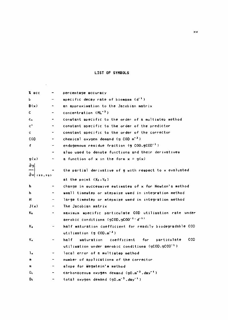
LIST OF SYl'1BOLS

percenta9e accuracy

specific decay rate of biomass (d- 1)

an approximation to the Jacobian matrix

concentration (Ml- 3)

constant specific to the order of a multistep method

constant specific to the order of the predictor

constant specific to the order of the corrector

chemical oxy9en demand (9 COD m- 3)

endo9enous residue fraction (9 C00.9COD- 1 >

also used to denote functions and their derivatives

a function of x in the form x = 9(x)

the partial derivative of 9 with respect to x evaluated

at t he p o i n t < Xo , Yo )

chan9e in successive estimates of x for Newton's method

small timestep or stepsize used in integration method

lar9e timestep or stepsize used in integration method

The Jacobian matrix

xv

maximum specific particulate COD utilisation rate under

aerobic conditions (9COO.gC00- 1 ·d- 11

half saturation coefficient for readily biode9radable COD

utilisation (9 coo.m-J)

half saturation coefficient for particulate

utilisation under aerobic conditions (9COO.gCOD- 1)

local error of a multistep method

number of applications of the corrector

slope for We9stein's method

~arbonaceous oxy9en demand (90.m- 3 .day- 1)

total oxy9en demand (90.m- 3 .day- 1)

COD

OUR p

r

Rs

6

So

Ss 1

Ssr

t

to

V

VSS

Xs 1

Xs r

Xs 1

Xs r

X

Xn IO I

y

y

Yn

oxy9en utilisation rate (90.m- 3 .day- 1 )

order of the integration method

volume of mixed liquor wasted per day (l.d- 1 )

influent wastewater flowrate <L3 r 1 )

settlin9 tank underflow flowrate (L3 T- 1 )

number of small timesteps in lar9e timestep

H = rh

rate of reaction of compound

system slud9e a9e (d)

XV i

change in successive estimates of x for Broyden's method

concentration of dissolved oxygen (gO.m- 3)

concentration of soluble substrate in the influent

C gCOD. m- 3 >

concentration of soluble substrate in the underflow

CgCOO.m- 3 >

acceleration factor for IJegstein's method

be9innin9 of time interval

Volume of reactor ( 1 )

concentration of volatile suspended solids C gVSS. m- 3 >

concentration of particulate biomass in the influent

CgCOO.m- 3 >

concentration of par ti cu 1 ate biomass in the underflow

C9COO.m- 3 >

concentration of endo9enous residue in the influent

C9COO.m- 3 >

concentration of endogenous residue in the under fl ow

(9COO.m- 3 >

concentration of particulate substrate in the influent

C9COD.m- 3 >

concentration of particulate substrate in the under fl ow

C9COO.m- 3)

vector of x values

initial estimate of the vector Xn

change in successive function values for Broyden's method

Arue growth yield

value of y at time tn C= yCxn ))

first derivative of y at time tn (= y' <xn>J

second derivative of y at time tn C= y'' <xn>J

predicted value of y

corrected value of y

xvii

GREEK CHARACTERS

p

0.

u

IJ.

d E

8

SUPERSCRIPTS

* +

SUBSCRIPTS

a

b

j

k

(p)

r

(0)

process rate expression (ML- 3 T- 1 )

maximum specific srowth rate

((9 COO cell srowth>.<s COD utilised)- 1 (day)- 1 ]

stoichiometric coefficient

chanse

partial derivative

error tolerance

safety factor for intesration method

denotes solution

denotes scaled variable

index denotes Ca) recycle

index denotes ( b) recyc 1 e

stream

stream

index denotes the it h reactor in a series

index denotes the j th compound in a series

index denotes the kt h reactor in a series

index denotes the pth iteration

index denotes the under fl ow rec ye 1 e stream

sravity settler

index denotes the initial estimate

XII i ii

from the

CHAPTER ONE

INTRODUCTION

The focus of this study is an evaluation of techniques for modelling and

simulation of biological system behaviour. Consideration is given to

both (1) the manner in which the mathematical model for a biological

system is presented, and (2) comparison of various numerical simulation

techniques.

The phenomenon of biological growth is harnessed in a wide variety of

applications. These may range from, for example, a laboratory

fermentation for the product ion of a pharmaceutical compound to the

treatment of municipal wastewater in a full scale activated sludge

process, The common feature in the various systems is biological growth,

even though the scale of operation and the final objectives of the

growth process may be very different. For example, in a fermentation

process, the objective is to maximise certain soluble products of growth

whereas in sewerage treatment an objective is to minimise the residual

soluble material. Whatever the objective, it is usefu 1 to be able

quantify system behaviour on the basis of a model of the process.

Because biological growth is the central feature in a 11 of these

applications, it is likely that very similar considerations wi 11 be

necessary in setting up and solving a mathematical model for any of the

systems,

A simulation program which can predict the response of a biological

system on the basis of a mathematical model is useful for a number of

reasons. For example:

Model development: A mathematical model incorporates a number of kinetic

and stoichiometric expressions which represent the biological

interactions. These expressions are based on hypotheses which are

proposed for the biological processes occuring within the system. In

order to test these hypotheses, spec i fie experiments are designed and

data on the system response is accumulated. This data can then be

1.2

compared with the predictions obtained from the model. In turn, the

biological model can be altered with the objective of improving the

predictive capacity. A simulation program is thus an indispensable tool

in facilitating the development and sophistication of a biological

model.

System evaluation and optimisation: A simulation program can be a useful

aid in analysing the operation of existing biological systems. If a

system model can provide accurate predictions of response behaviour,

then these predictions can be compared to observed responses. Any

discrepancies can be useful in identifying problems in system operation.

An accurate and representative computer model can also be used to

optimise the performance of existing systems. Various operating

strategies can be proposed and rapidly tested without having to resort

to potentially difficult practical evaluation.

System design: A simulation program can be a useful tool for the design

engineer. With the aid of an accurate and representative computer model,

proposed system designs and configurations can be evaluated rapidly. In

addition, a dynamic model can provide valuable design information which

is usually only available through empirical estimates. For example, a

parameter such as peak oxygen uti 1 isation rate in an activated sludge

system could be obtained directly from the simulation program run under

time-varying input patterns. This means that the peak aeration capacity

can be quantified accurately traditional design methods rely on

empirical estimates.

Control strategy development: A simulation program allows the rapid and

efficient evaluation of control strategies in a manner similar to

evaluation of system designs. Strategies can be tested and compared in

an economical way that reduces the need for field evaluation.

Having identified some of the reasons why it is useful to model

biological system behaviour, it is now possible to define certain of the

requirements ip a computer program for simulating system behaviour.

Amongst these are the following:

1.3

The program should be able to simulate the response behaviour in the

types of system configuration encountered in practice. A typical

biological reaction system configuration would consist of a series of

interconnected reactors. In certain applications, the last reactor in

the series would be followed by a sedimentation tank. Mixed liquor

will usually flow sequentially by gravity from reactor to reactor, and

internal recycles may convey 1 iqour to upstream reactors, Influent to

the system may be distributed to any of the different reactors. If a

sedimentation tank is included, the underflow may be recycled to any

of the reactors.

In model 1 ing the system described above, the general approach is to

consider each reactor as a completely-mixed stirred tank CCSTR), with

individual units being connected to the others by streams. These

interconnected modules form the flowsheet which is used as the basis

for the simulation program. 111

- The simulation program should be capable of analysing both steady

state and dynamic behaviour. In a steady state situation, the system

operates under constant flow and load conditions. Under a dynamic

regime, influent flow and/or concentration will vary with time. In

certain situations such as a wastewater treatment plant, the inputs

will vary with time in a cyclic pattern which is repeated closely from

day to day. In this case, a useful facility of a computer simulation

program is the ability to predict the steady state cyclic response

under the expected cyclic input pattern.

The computer program should be structured in such a way that

refinements to the biological model can be made with a minimum of

( 1 I Plug flow reactors, such as oxidation-ditch type activated sludge systems, can also be modelled using this approach. The plug flow reactor is considered to be 111ade up of a number of small CSTR's in series. This is a standard approach adopted in chemical engineering process simulation.

1.4

disruption of the program code. This is to facilitate efficient model

evaluation and development.

- The numerical techniques utilised by the computer program should

provide accurate solutions to both the steady state and the dynamic

problem. The numerical methods should be efficient and economical in

terms ·of computer time, as well as being stable and robust enough to

handle a wide variety of system configurations and kinetic models.

Some mathematical model is required as a basis for the analysis of

modelling and simulation techniques appropriate for biological systems.

In this investigation, a model of limited scope has been selected. This

has the advantage of being easily manageable in terms of both analysis

and presentation of the techniques. Nevertheless, it has been attempted

to select a model which is fully representative of the range of

biological growth applications. The model which has been adopted is a

simplified version of the activated sludge system model of the

International Association for Water Pollution Research and Control

<IAWPRC). Therefore, to a certain extent, the analysis is specific to

the activated sludge system. Nevertheless, because this model

incorporates features common to a range of biological processes, the

results can be extended readily to other systems.

CHAPTER TWO

MATHEMATICAL DESCRIPTION OF BIOLOGICAL REACTION SYSTEMS

2.1 INTRODUCTION

A comprehensive mathematical model for the simulation of biological

system behaviour must account for a large number of reactions between a

large number of components (compounds). In this presentation, the

reactions will be referred to as processes, where processes act on

certain coapounds in the system, and convert these to other compounds.

The set of distinct biological processes and the manner in which these

act on the group of compounds constitute the biological model. The model

should quantify, for each process, both the kinetics (rate-concentration

dependence) and the stoichiometry (effect on the masses of compounds

involved) (Henze et al, 1987).

Once a mode 1 has been for mu 1 ated for a bi o 109 i ca 1 system, s i mu 1 ati on of

the system response involves two principal steps. Firstly, the reactor

configuration and the flow patterns need to be specified. Once this

information is fixed, it is -possible to complete mass balances over each

reactor for each compound. Assuming that the system operates at constant

temperature, this quantifies the behaviour of each compound in the

system. The concentrations of these "compounds" constitute the state

variables (dependent variables>. The mass balances make up the state

equations which relate the dependent variables to the independent

variables such as reactor volume. The mass balances form a set o~

simultaneous non-linear equations which, when solved, characterise the

system behaviour. 111 The simultaneous solution of these equations thus

provides values of the state variables at points in space (different

reactors) and time (where there is a time-varying input to the system).

In this way, the change of state of the system is related to the

I l I The equations are usually non-linear because the kinetic expressions for biological systems generally are non-linear.

2.2

transport (input and output) and conversion

occurring within the system.

<reaction) processes

At this point it is worth noting certain characteristics of biological

reaction systems which distinguish these from most other applications in

the chemical process industry:

A feature commonly encountered with biological systems is that the

process occurs

reactors. 121

in a series of completely mixed stirred tank

- An identical set of reactions often takes place in each reactor in the

system. For example, in a series of aerobic activated sludge reactors,

the behaviour in each reactor is governed by the same kinetic and

stoichiometric expressions. The only difference between the reactors

would be the values of the state variables, the reactor volumes and

the flow terms.

The response of biological systems is often governed largely by the

effect of recycles.

These features of biological systems are not usually encountered in

operations in the chemical process industry. Those systems are generally

made up of a di st i net set of unit operations. Therefore, each reactor

unit is governed by a different collection of reaction equations i.e. a

different model. Also, the magnitude of the recycles and feedbacks is

generally small. These distinguishing features of biological systems;

demand that specific consideration be given to their simulation.

I 2 I As noted earlier, certain reactor configurations such as oxidation ditch type systems for wastewater treatment may not appear to fit the description given here, as these are essentially plug flow reactors with recycle, and are not divided into distinct zones. However, these systems can be modelled as tanks-in-series systems by considering the plug flow zones to be made up of a number of small CSTR 1 s in series. This is a standard approach adopted in chemical engineering process simulation.

2.3

2.2 MODEL REPRESENTATION

An important part of the simulation process is a clear and flexible

representation of the model itself. Because a model may incorporate a

number of different components and a large number of biological

conversion processes, one convenient method of presentation is a matrix

format. -

The matrix method for model presentation described here is based on the

approach to chemical kinetic modelling of Petersen (1965). In the

context of biological systems, the method has been utilised by the

IAWPRC Task Group on mathematical modelling in wastewater treatment

design (Henze et al, 1987). The matrix representation ensures clarity as

to what compounds, processes and react ion terms are to be incorporated

and allows easy comparison of different models. In addition, the method

facilitates transforming the model into a computer program.

2.2.1 Setting up the aatrix

Table 2.1 presents, in matrix format, the essential components of a

simple Monod-Herbert model for aerobic microbial growth on a soluble

substrate, accompanied by organism death.

The first step in setting up the matrix is to identify the compounds of

relevance in the model. The Monod-Herbert model quantifies the growth of

the biomass component (Xe) at the expense of the soluble substrate

component (Se). By keeping track of Xe and Sa, it is possible tp

calculate the oxygen requirement, so oxygen <So> can be included as a

third component. The compounds are presented as symbols across the top

of the table, and are defined (with units) at the bottom of the

corresponding matrix columns. The index "i" is assigned to the range of

compounds. In this case, "i" ranges from 1 to 3 for the three compounds

considered in this simple model. 131

( J) The recommended symbol notation of the IAWPRC has been fol lowed: namely, X for particulate matter and S for soluble materials. (Grau et al, 1982>

2.4

Component i 1 2 3 Rate expressions

j Process x. Sa So

-1 (1-Y) s, 1 Growth 1

,.. x. -- - Ll

y y <Ka+Ss)

-2 Decay -1 1 b x.

Observed conversion Kinetic paraaetera: rates ( ML- 3 r 1 > r1 = I V1, P, Maximum specific

growth rate: ,.. Ll ,...

C

Stoichiometric 0 Half saturation u para•etere: UJ constants: Ks, Ko True growth yield: y :> Spec i fie decay rate: - b ....

C:,., ,., ,., C) I

I I UJ ....I ....I UJ ....I z .... .... ,...

Cl) ,... C:,... C Cl) C 0:::0 zo C: 0 .... o UJ u :cu Cl) u C> I 0 .... al .... >- .... - :::> >< al :c Cl) :c 0 :c

Table 2.1 The Monod-Herbert model showing process kinetics and

stoichiometry for heterotrophic bacterial growth in an aerobic

environment

2.5

The second step in developin9 the matrix is to identify the biolo9ical

processes occurrin9 in the system. These are conversions or

transformations which affect the compounds considered in the model. Only

two processes take place in this simple model aerobic 9rowth of

or9anisms at the expense of soluble substrate, and or9anism decay. These

are itemised one above the other at the left of the matrix. The index

"j" is assi9ned to the range of processes: in this case "j" can only

assume a value of 1 or 2.

The kinetic expressions Crate equations) for each process are recorded

down the right hand side of the matrix in the appropriate row. These are

9iven the symbol PJ with j denotin9 the index of the biolo9ical process.

The kinetic parameters incorporated in the rate expressions are defined

at the lower ri9ht corner of the matrix.

The elements within the matrix comprise the stoichiometric coefficients,

VtJ, which define the mass action relationship between the components in

the individual processes. For example, aerobic 9rowth of heterotrophs

(+1) occurs at the expense of soluble substrate C-1/Y): oxy9en is

uti 1 i sed in the metabo 1 i c process (-( 1-Y) /Y). The sto i chi ometr i c

parameters are defined at the lower left of the table.

The stoichiometric coefficients VtJ are 9reatly simplified by workin9 in

consistent units: in this case, all concentrations are expressed as COD

equivalents. Provided consistent units have been used, continuity may be

checked from the stoichiometric parameters by movin9 across any row o~

the matrix. With consistent units, the sum of the stoichiometric

coefficients must be zero Cnotin9 that oxy9en uptake is equivalent to

ne9at ive COD).

The sign convention used in the matrix is "ne9ative for consumption" and

"positive for production". Co9n i sance must be taken of the units used in

the rate equation. For example, the rate equation for aerobic growth of

biomass, P1, is written as a bioaasa growth rate (not as a substrate

utiliaation rate) and has units of <ms cell COD 9rowth)(m9 substrate COD

2.6

utilised)- 1 (day)- 1 • The stoichiometric values are thus normalised with

respect to the bioaass concentration i.e. for growth, the stoichiometric

coefficients for Xe and Sa are 1 and -1/Y respectively, and not Y and

-1.

2.2.2 Use in aass balances

Within a aystea boundary, the concentration of a single compound may be

affected by a number of different processes. An important benefit of the

matrix representation is that it allows rapid and easy recognition of

the fate of each component, which aids in the preparation of mass

balance eQuations.

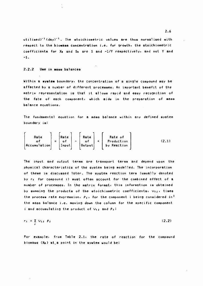
The fundamental eQuation for a mass balance within any defined system

boundary is!

[Rate l [ Rate l [ of - of + Input Output

Rate of l Production

by Reaction (2 .1)

The input and output terms are transport terms and depend upon the

physical characteristics of the system being modelled. The incorporation

of these is discussed 1 ater. The system react ion term (usual 1 y denoted

by ri. for compound i) must often account for the combined effect of a

number of processes. In the matrix format, this information is obtained

by summing the products of the stoichiometric coefficients, vi.,, times

the process rate expression, P,, for the component i being considered in I

the mass balance i.e. moving down the column for the specific component

i and accumulating the product of vi., and P,:

ri. = I Vi. J P J (2.2)

For example, from Table 2.1, the rate of reaction for the compound

biomass <Xa> at.a point in the system would be:

u Sa rx1 = -----· Xa - b Xa

( Ka + Sa>

2.7

(2.3)

Similarly for the component soluble subst~ate (Sa>:

rs• = -1

y u Sa -----·Xa

(Ka + Sa)

and for dissolved oxygen (So):

rs o = (1-Y>

y u Sa

-----·Xa - b Xe ( Ks + Sa)

(2.4)

(2.5)

To create the mass balance for any component within a given system

boundary (e.g. a completely mixed reactor) the conversion rate, r,,

would be combined with the appropriate advective terms (input and output

flow) for the particular system: this is not shown here as the aystem is

not yet defined. 141

2.2.3 Switching functions

At this point, it is worth introducing an aspect of the kinetic

expressions which is often useful namely "switching functions".

Consider the aerobic growth of biomass. In Table 2.1, the Monod growth

rate equation has been utilised:

Pt = U Sa

-----·Xe ( Ka + Sa)

(2.6)

In an environment where the dissolved oxygen concentration <So> is zero

(or perhaps close to zero), the rate of this aerobic process should also

decrease to zero. Mathematically, this can be achieved by multiplying

the Monod rate expression by a "switching" factor which is zero when So

I 4 I The system reaction rate or conversion rate, r,, may be of interest on its own. For example, Eq (2.5) defines the "rate of production" of' So: therefore -rao defines the oxygen utilisation rate at a point within the .system. This parameter is often of' interest in aerobic systems.

is zero, and unity when the environment is aerobic. In this case,

convenient to write the switching function in the form:

So

< Ko + So >

where Ko = switching constant of small magnitude

(say 0.1 mg0/1)

The process rate equation then becomes:

u Ss Pt =

< l<s + Ss >

So Xs

( Ko + So)

2.8

it is

(2.7)

(2.8)

IJith this "switching function" operating on the growth rate equation,

when So is zero the value of the function is zero, and the process rate,

Pt, will be zero. However, if So is say 1 mg0/1 then the value of the

switching function is close to unity and the process rate will then be

that given by the Monod equation. In this way, the process of aerobic

9rowth is switched "on" or "off" automatically by the model dependin9 on

the dissolved oxy9en concentration. The selection of a small value for

Ko means that the value of the switchin9 function decreases from

near-unity to zero only at very low So values i.e. when the 0.0. value

decreases below, say 0.2 mg0/1. However, the function is mathematically

continuous, which helps to eliminate problems of numerical instability

in simulating system behaviour: such problems can arise if the rate is

switched "on" and "off" discontinuously.

In certain situations, the switching "off" of one process may be linked

to the switching "on" of another. If, for example, the oxygen input to a

nitrifying activated sludge system were terminated periodically, there

would be a switch from aerobic to anoxic growth. The latter process is

governed by kinetic and stoichiometric expressions which differ from

those for the aerobic growth process. To account for this phenomenon in

a single model, the rate equations for aerobic and anoxic growth can be

multiplied by the appropriate switchin9 functions as follows!

2.9

Observed Pa•robic So = Pa•robic

<Ko + So> (2.9)

. [ So l Observed Pano•ic = Pano•ic 1 -<Ko + So>

Ko = Pano•ic

C Ko + So> (2.10)

In this instance, it is apparent that the selection of Ko will influence

the point at which there is a switch from aerobic to anoxic growth, and

vice versa. That is, Ko now influences the model predictions and is not

only serving a mathematical objective. Therefore, whenever switching

functions are utilised, care should be taken in the selection of the

magnitude of the switching constant <Ko here) to ensure that the model

predictions are not incorrectly biased.

The consequence of using switching functions to switch between processes

within a model should be hi9hli9hted. The example of anoxic and aerobic

growth illustrates how switching functions enable incorporation of

qualitative changes in system behaviour within a single model. Without

switching functions, different models would be required to simulate the

behaviour either in an aerobic or an anoxic environment.

2.3 BIOLOGICAL NOOEL USED IN THIS STUDY

A biological model of limited complexity has been selected as the

"demonstration" model in this study. That is, only a limited number of

compounds and processes have been incorporated. The objective of

limiting model size has been to enable rapid evaluation of numerical

modelling techniques. Despite its limited size, however, the model

nevertheless incorporates a range of characteristics encountered in

biological systems.

Table 2.2 presents the 1 imited model in matrix format. This model is a

reduced version of that proposed by the IAWPRC Task Group for mathe-

2.10

Component i 1 2 3 4 5 Rate expressions

j Process x. XE Xa Sa So

-1 Cl-Y> Sa So 1 Growth 1

,... Xs -- - --- u

y y C Ka +Ss) ( Ko +So)

2 Decay -1 f ( 1-f) b x.

KH ( Xa /Xa) 3 Solubilisation -1 1 x.

< Kx + ( Xa /Xe ) )

Stoichiometric UJ ~ Kinetic parameters: parameters: ~ 0

(/) <t: 0 (/) UJ IX: u Maximum specific <t: :::, ~ UJ

True growth J: 0 (/) ~ UJ I growth rate: " 0 .... a:i <t: ::> u yield: y .... (/) :::, IX: .... Maximum a:i UJ (/) ~ ~

Endogenous residue IX: (/) < l'I solubilisation WM l'I WM al l'I o, fraction . f ~. (/) I ~ I ::) I W...J rate: KH . <t: ...J :::, ...J < ...J (/) ...J z

...J 0 ...J ..... ~ Half saturation :::,~ z~ :::, ~ w~ 0 uo WO uo ...JC zo constants: Ks , Ko , Kx .... 0 00 .... o al 0 WU ~ u Ou ~u ::::>u 0 I Specific decay ex: ..... a ..... ex: ._. ...J ..... >- ..... <t: z < 0 X rate: b Q.. J: w J: Q.. J: (/) J: 0 J:

Table 2.2 The reduced IAWPRC model for utilisation of carbonaceous

material in an aerobic activated sludge system

2.11

matical modellin9 in wastewater treatment desi9n (Dold and Marais, 1985)

<Henze et al, 1987). The model incorporates only those features which

relate to the utilisation of' carbonaceous material in an aerobic

activated slud9e system.

Five compounds are identified in the demonstration model. These are:

- heterotrophic or9anism mass <Xe)

- endo9enous residue <XE)

- particulate biode9radable substrate (Xs)

- soluble biode9radable substrate (Ss)

- dissolved oxy9en (So)

Three processes operate on the compounds in a manner defined by the

stoichiometry and the process rate equations:

Aerobic 9rowth of heterotrophs: Soluble substrate (Ss) is uti 1 ised for

9rowth by the heterotrophic or9anisms (Xe). There is an associated

utilisation of' oxy9en <So). The process is modelled by the Monod

expression to9ether with a switchin9 function which reduces the rate to

zero in the absence of' oxy9en.

Death of heterotrophs: Or9anism decay is modelled accordin9 to the

"death-re9eneration" hypothesis. The heterotrophic or9anism mass dies at

a certain rate: a portion of' the material from death is non-de9radable

(f') and adds to the endo9enous residue (XE) while the remainder (1-f')

adds to the pool of' biode9radable particulate COO (Xs>.

I

Hydroly•is of particulate COO: Biode9radable particulate COD in the

influent is assumed to be enmeshed in the slud9e mass within the system.

The enmeshed material is broken down extracellularly, with the products

of breakdown addin9 to the pool of' readily biode9radable substrate <Ss)

available to the organisms f'or synthesis purposes. This

"hydrolysis/solubilisation" process is modelled on the basis of'

Levenspiel's surface reaction kinetics <Levenspiel, 1972).

2 .12

A number of features incorporated in this model, and which may be

encountered with other biological systems, should be noted. These are:

Dual •ubstrate: The model distinguishes between soluble and particulate

biodegradable influent material, and the manner in which these are

removed in the system.

Non-linear expressions: The non-linear nature of certain of the process

rate equations introduces non-linear terms into the mass balance

equations. This aspect influences the numerical techniques for solution

of the simulation problem.

Single and aeries reactions: Utilisation of soluble substrate directly

by the organism is modelled as a single reaction. However, utilisation

of particulate material occurs in two steps: hydrolysis to soluble

substrate followed by utilisation of the soluble substrate. This

sequence constitutes a series reaction.

Bulk versus surface concentration teras: Generally, process rate

expressions are formulated in terms of the bulk concentration of certain

species in the system (i.e. the mass per unit system volume). For

example, the concentration of soluble substrate (Ss> as used in the

Monod growth rate expression is given by the mass of Ss in the system

divided by the volume of the system. However, in certain cases, the

basis for quoting concentration is some parameter other than the system

volume. For example, hydrolysis of particulate substrate is modelled as

being dependent on the concentration of part i cu 1 ate mater i a 1 adsorbed1

onto the organism mass i.e. the surface concentration. The ratio of two

bulk concentrations <X1/Xs> is used to approximate the surface

concentration, and this term appears in the rate expression.

2.4 SETTING UP THE MASS BALANCE EQUATIONS

In a system consisting of a series of completely mixed reactors, the set

of equations de.fining the state of the system is obtained by performing

a separate mass balance over each reactor for each compound. Where a

2.13

solids/liquid separator, such as a '3ravity settlin'3 tank, is included in

the confi'3uration, an additional set of mass balance equations is

required.

2.4.1 The reactor

Consider a sin'3le component in the ith reactor in a series of n

completely mixed reactors (Fi'3 2.1)!

The inputs to the reactor could comprise some or all of the followin'3!

(i) an influent feed stream at a flow rate Q, .. d and a concentration

(ii) flow from the previous reactor [(i-1>th) in the series, at a flow

rate Q,-1 and a concentration C,-1:

(iii) a mixed liquor recycle (a) from the kth reactor in the series, at

a flow rate Q. and a concentration Ck:

(iv) underflow from the settlin'3 tank at a flow rate Qr and a

concentration Cr.

Output streams from the ith reactor could comprise some or all of the

fol lowin'3!

(i) flow from this reactor to the next reactor [(i+1)th l in the series

at a flow rate Q, and a concentration C,: (ii) a mixed liquor recycle (b) out of this reactor at a flow rate Qb

and a concentration C,: Ci ii) a slud'3e wasta'3e stream may be withdrawn from the reactor at a

rate qw and a concentration C, 1'

1

The reaction terms are obtained as described previously, by summin'3 the

products of the stoichiometric coefficients and the process rate

expressions for the particular component bein'3 considered. These

IS I Biolo'3ical slud'3e is withdrawn to prevent a build-up of so.lids in systems jncorporating a solids/liquid separator. In this presentation, waste liquor will be withdrawn only from the last reactor in the series.

2 .14

conversion terms are combined with the flow terms to create the mass

balance equations.

Substituting in Eq (2.1), the mass balance for a single compound in the

ith reactor in a series is!

- Q.,C, - qwC, + rV,

where V, = volume of the ith reactor (l3 }

C = concentration (Ml- 3)

Q = flow rate <L3 r 1 >

qw = wastage rate CL3 T- 1 >

(2.11}

r = rate of reaction or conversion rate of the compound

(positive for production) <ML- 3 r 1 >

= I V P J

2.4.2. The solids/liquid separator

In certain circumstances, the output from the last reactor in the

biological system passes to a solids/liquid separation device (often a

gravity settler}. This is usually with the intention of being able to

maintain an organism retention time in excess of the hydraulic retention

time and for maintaining a solids-free effluent. In this presentation,

it has been assumed that the process which occurs in the settling tank

is merely one of physical concentration i.e. no reaction takes place. In1

this way, the settling tank is treated as a separation point with no

hold-up. Also, the settling tank is considered to operate at 100 percent

efficiency. This means that the overflow from the settling tank

comprises only soluble material and all particulate compounds entering

the vessel are recycled back to the chain of reactors. Mass balances

over the settler must therefore distinguish between particulate and

soluble compounds.

2.15

Figure 2.2 illustrates the f'low terms associated with a settling tank

situated at the end of' a series of' n reactors. These are:

(i) f'low f'rom the last <nth) reactor at a f'low rate CQ, .. d + Q, - qw)

and a concentration Cn:

(ii) overf'low f'rom the settling tank at a rate of' CQ, .. 41 - qw) and a

concentration of' Cn f'or soluble material and C = 0 f'or particulate

111aterial:

(iii) underf'low f'rom the settling tank, at a f'lowrate of' Q, and a

concentration C,.

Mass balances f'or the particulate and soluble compounds are as f'ollows:

Particulate:

Soluble:

With Cn = C, f'or soluble compounds, this yields the trivial mass

balance:

Cn - C, = 0

2.4.3 Dissolved oxygen mass balance

(2.12)

(2.13)

Although dissolved oxygen <So> is included in the matrix, a mass balance1

f'or So will not usually be required. This is because the oxygen input to

a reactor is generally regulated externally in order to maintain the

dissolved oxygen concentration at some constant value. The reason f'or

including So is that it allows computation of' the oxygen utilisaiton

rate (-rao>, an important parameter in modelling aerobic behaviour.

INFLUENT Qf••••Cf•••

FLOW FROn (i-1)t• REACTOR IN SERIES Qt-1-,Ct-t

nIXED LIQUOR RECYCLE (b) OUT OF i 111

REACTOR Q,, Ct

REACTOR i

2.16

nIXED LIQUOR RECYCLE <a> OUT OF k111

.-----REACTOR Q •• c.

---nIXED LIQUOR WASTAGE q11,Cr

a---.FLOW TO (i+1>t• REACTOR IN SERIES Q, I Ct

.__ ___ RAS RECYCLE Q,. ,C,.

Figure 2.1 Schematic representation of the ith reactor in a series of n

completely mixed reactors

FLOW FROM LAST REACTOR IN SERIES <Qf••• + Qr - q11>,C.

UNDERFLOW Q,. I Cr

EFFLUENT (Qf••• - q11>,C. FOR SOLUBLE

0 FOR PARTICULATE

Figure 2.2 Schematic representation of a solids/liquid separator at the

end·of a series of reactors

2 .17

2.5. A CASE STUDY

Consider the system of Fig 2.3 comprising a single aerobic reactor and a

settling tank. Underflow from the settling tank is returned to the

reactor. The system is described by eight mass balance equations, one

for each of the compounds, Xa, XE, Xe, and Sa in the reactor and in the

settling tank underflow, respectively. The eight simultaneous equations

comprise a set of four non-1 inear ordinary differential equations for

the reactor and four algebraic equations for the solids/liquid

separator.

Reactor:

dXa V -- = Q,Xa,t + QrXB,r - CQ1+Qr >Xa - b Xa V +

dt

dXs V -- = Q, Xs, , + Qr Xs , r - ( Q, +Qr ) Xe +

dt

C 1-f> b Xa V -

0. Ss Xe ( Ks +Ss )

V

(Kx+Xs/Xe)

(2.14)

(2.15)

V (2.16)

0. y

Xa Ss KH Xs V + ----- V (2.17)

<Ks+Ss) CKx+Xs/Xa)

Solids/liquid separator:

( Q, + Qr - qw ) Xe = Qr Xe , r (2.18)

(2.19)

( Q, + Qr - Qw ) Xe = Qr Xe , r (2.20)

• Sa = Sa, r C 2. 21>

2.18

WASTAGE, q11

INFLUENT, Q,

Qr

Figure 2.3 A case study: a single aerobic reactor with settling tank

2 .19

2.6 CLOSURE

For the steady state situation, where the system operates under

conditions of constant influent flow and load, the derivative terms in

the reactor mass balance equations fall away. This reduces the single

reactor-plus-settler example problem to a set of eight simultaneous non

linear _algebraic equations. In the dynamic situation, the problem

remains one of solving the system of four non-linear ordinary

differential equations and four algebraic equations. Solution procedures

for solving the sets of equations resulting from the steady state and

dynamic situations necessitate specific considerations in each case.

The steady state problem involves finding a single value for the

concentration of each compound in each reactor and in the underflow

recycle stream which satisfies the set of algebraic equations. Because

the biological reactions introduce non-1 inear terms into the equations,

the solution cannot be found directly and iterative techniques must be

employed. These techniques range in complexity from simple successive

substitution (with or without acceleration) to the various Newton-type

methods. The success and efficiency of the different techniques is

determined principally by the degree of non-linearity in the equations.

Under dynamic conditions, a set of coupled ordinary differential and

algebraic equations describe the change in concentration of each

compound in each reactor with time subject to variations in the input

pattern. Because the biological system incorporates reactions involving

both soluble and particulate compounds at a range of concentrations, the1

system will exhibit dynamics varying from fast to slow for different

compounds. Therefore, utilisation of an integration technique that

exploits the differing dynamics exhibited by the compounds in a

biological system is indicated.

In both the steady state and dynamic situations, the objective has been

to identify numerical techniques which take advantage of the particular

characteristics of the equations describing the system.

exploring the nature of their non-linearity, and exploiting the specific

2.20

dynamics of the biolo9ical reaction behaviour, it has been possible to

identify techniques appropriate for either the steady or the dynamic

situation.

CHAPTER THREE

MODELLING OF THE STEADY STATE CASE

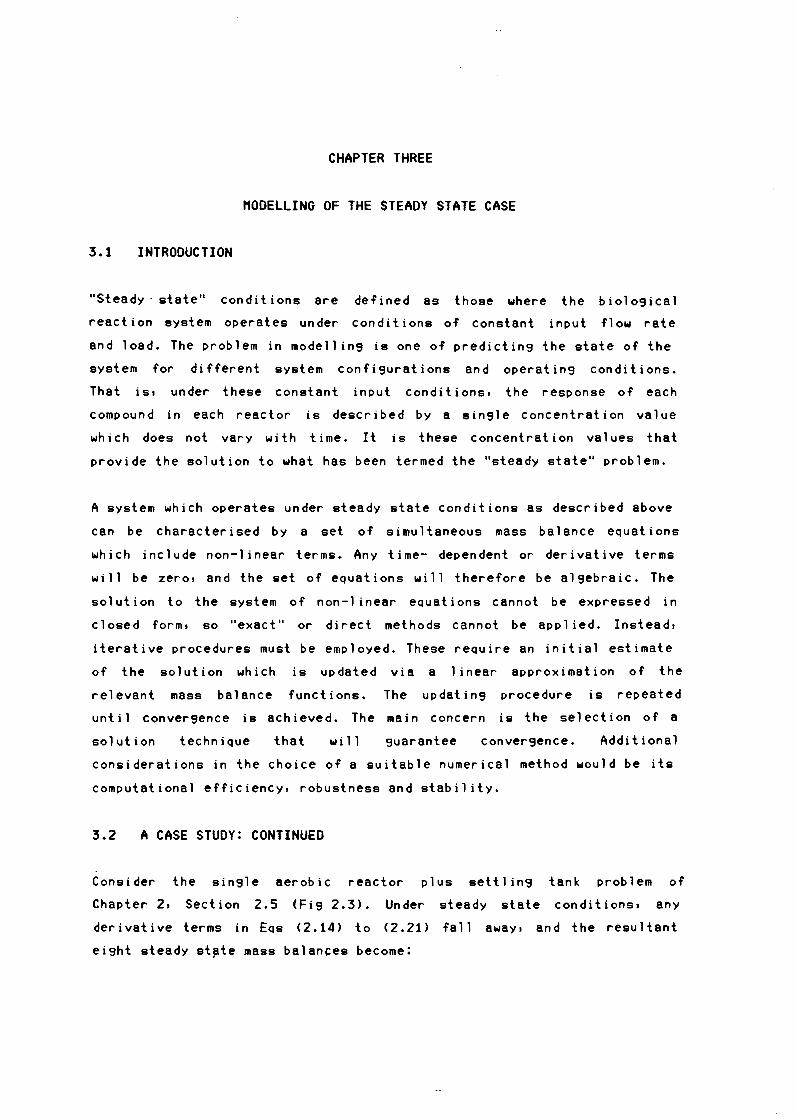
3.1 INTRODUCTION

"Steady - state" conditions are defined as those where the biological

reaction system operates under conditions of constant input flow rate

and load. The problem in modelling is one of predicting the state of the

system for different system configurations and operating conditions.

That is, under these constant input conditions, the response of each

compound in each reactor is described by a single concentration value

which does not vary with time. It is these concentration values that

provide the solution to what has been termed the "steady state" problem.

A system which operates under steady state conditions as described above

can be characterised by a set of simultaneous mass balance equations

which include non-linear terms. Any time- dependent or derivative terms

will be zero, and the set of equations will therefore be algebraic. The

so 1 ut ion to the system of non-1 i near equations cannot be expressed in

closed form, so "exact" or direct methods cannot be applied. Instead,

iterative procedures must be employed. These require an initial estimate

of the solution which is updated via a linear approximation of the

relevant mass balance functions. The updating procedure is repeated

until convergence is achieved. The main concern is the selection of a

solution technique that will guarantee convergence. Additional

considerations in the choice of a suitable numerical method would be its

computational efficiency, robustness and stability.

3.2 A CASE STUDY: CONTINUED

Consider the single aerobic reactor plus settling tank problem of

Chapter 2, Section 2.5 (Fi9 2.3>. Under steady state conditions, any

derivative terms in Eqs (2.14) to (2.21) fall away, and the resultant

eight steady st,te mass balances become:

Reactor:

Qr Xe , r - C Q, +Qr ) Xe - b Xe V + U Ss Xe

( Ks +Ss )

Qr Xs , r - CQ, +Qr ) Xs + C 1- f) b Xe V -

(Kx+Xs/Xe)

Q QrSs,r - CQ,+Qr)Ss -

y Ss Xe

( Ks +Ss ) V +

(Kx +Xs /Xe)

Solids/liquid separator:

< Q, + Qr - qw ) Xe - Qr Xe , r

< Q, + Cr - qw ) Xs - Qr Xs , r

Ss - Ss, r

3.2

V = - Q, Xe, 1 C 3 .1)

(3.2)

V = - 01 Xs,, (3.3)

V = - Q, Ss, 1 (3.4)

= 0 (3.5)

= 0 (3.6)

= 0 (3.7)

= 0 (3.8)

These equations may be written in the form f(x) = 0 where x is the

vector of state variables:

X :

Xs, r

Ss, r

Some insight into appropriate numerical solution procedures for the

steady state prob 1 em may be 9a i ned by represent i n9 the equations in a

matrix format •.

3.3

3.3 THE STEADY STATE MATRIX

The matrix representation is used here because it 9ives a concise

summary of the steady state problem. It shows, amonsst others, features

such as feed distribution, the flow links between reactors and the

conversion processes, in a "sraphical" manner.

Consider how the ei9ht simultaneous steady state mass balance equations

[Eqs (3.1) to (3.8)] of the case study are transformed into the matrix

format in Fis 3.1. The equations are expressed in the form:

A X = B (3.9)

The X Vector: Equations (3.1) to (3.8) are mass balances for the ei9ht

state variables Xe, XE1 •••• ,Xs,r and Ss,r• These state variables form

the X vector, which is the solution to the steady state problem.

The B Vector: This is the "feed vector". It contains the elements of the

ri9ht hand sides of Eqs (3.1) to (3.8). Each term is the influent mass

input rate of the correspondin9 compound into the particular zone

(nesative value). In this case, the first four values are the influent

mass input rates of Xe, XE, Xs and Ss into the reactor. For example,

-Qi Xe, 1 is the input rate of Xe into the reactor. The last four values

are the influent inputs into the settler (zero here).

The A Matrix! The A matrix contains the reaction and flow terms which

characterise the particular activated slud9e system confi9uration. It is

of interest to note how the non-1 inear terms are handled. Consider how

Eq (3.1) is inserted in the top row of the matrix. The linear terms can

only be placed in one location. These are -CQ1+Qr>, Q, and -bV. However,

the non-linear term, cQ Ss Xe V/ <Ks+Ss)) can be handled in two ways:

- (U Ss V/ (Ks+Ss)) in the Xe location

or

- CU Xe V/ <Ks+Ss» in the Ss location

In this case, the second option has been used.

0

0

:>

I -;: . "' +

<:l . "'

-0 +

0 I

-0

:> + :> ... ci ...

I ... I

Fi9ure 3.1

3.4

0 -I

0 0 I

0 I

0 I

:> -.:I

-o .;; + -+ .:lo

I

9 I >-

-:> . :> - " -o - I . . >< 0 >< + ' ' .,J. ;: + .,J. . ->< 0 +

I + - ,:; ci ,:; I

I

-" " I

0 +

0 I

-:>

. " I ...

:: 0 I + - ci

I

A matrix representation of the mass balance equations for a

single reactor and settling tank system.

3.5

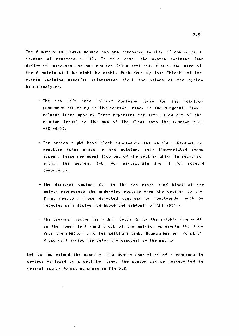
The A matrix is always square and has dimension (number of compounds * (number of reactors + 1)). In this case, the system contains four

different compounds and one reactor (plus settler>. Hence, the size of

the A matrix wi 11 be eight by eight. Each four by four "block" of the

matrix contains specific information about the nature of the system

being analysed.

- The top left hand "block" contains terms for the reaction

processes occurring in the reactor. Also, on the diagonal, flow

related terms appear. These represent the total flow out of the

reactor [ equa 1 to the sum of the flows into the reactor i.e.

- (QI +Qr ) ] •

- The bottom right hand block represents the settler. Because no

reaction takes place in the settler, only flow-related terms

appear. These represent flow out of the settler which is recycled

within the system. (-Qr for particulate and -1 for soluble

compounds).

The diagonal vector, Qr, in the top right hand block of the

matrix represents the underflow recycle from the settler to the

first reactor. Flows directed upstream or "backwards" such as

recycles will always lie above the diagonal of the matrix.

- The diagonal vector CQ1 + Q, >, (with +1 for the soluble compound)

in the lower left hand block of the matrix represents the flow

from the reactor into the sett 1 ing tank. Downstream or "forward"

flows will always lie below the diagonal of the matrix.

Let us now extend the example to a system consisting of n reactors in

series, followed by a settling tank. The system can be represented in

general matrix format as shown in Fig 3.2.

... a L

'"O O &.. 0 .... - .. • C-.. U LL - • • • ..C L ...

• L "V o .. 0 . ... - .. • C u

u.. - t,. ..c .. ..- L

• L "Vo- 0 .. .. .M .. .. C U

L1. - ... ..c .. ..- L

-v o ·c t ........ t, C t, c.,

u.. - •• ... .. L

3.6

BE---...... ,:,:~~

• L 0 L 0 L .. ... ·- ... ... ... ..... ..c • ~

..... L • ... 0 ... u ..... • t,..c L "' ... ;;:

... C • 0 • L

-; .. L .. 0 L • ... .. .. .. ... > u ..c • C 0 ... • 0 L L

u .. C -

"' 0 ... u C w

"'

Figure 3,2

• L L 0 .. 0 L- ... . ... .. u

... ..c • .. .. ... .. ~ • L

0 ,., ....... u..c :.. .. ... "'

• -· C . .,-_ L 0 ·-0 -; ·- L u ..c ... • 0 ...... .. u L • ..... ... ..c • .. .. ..c u .. . ... .. > u ... • "' 0

0 L C 0 ..

L 0 L C L ~ ... u .. ·-

C . 0 ·-.. ·- L • • 0 L • ..... .. 11..C u > u .... C 0 .. 0 L C L u .. ·-

"' "' 0 0 ... ... u u C C w w "' "'

C 0

• L .. > C 0 u

. -;.. :.. -: L - 0 a .. - ...

0 ..c u ii: ... .. • ..c .. . ... L

0 L 0 ~ ...

"' o-... -u + c-w-"'

-I 0 I

0 I

0 I

.. -..c L C .. ... 0 • ·- ... • C L • u • 0 0 • .. " .. .. ... .:: .. ..c C u ..c ... L ... -0 ... • 0::; L .. a. A C L o- ......

C .. LL •

C U z

"' -0 ..J"' ... ... z u >- C C W>-W <I>

"'

"' z C ... C>

~ ..J .... .... w "'

C

"' 0 ... u C w

"'

"' 0 .... u C w

"'

"' 0 ... u C w

"'

"' 0 .... u C w "'

The steady state matrix representation of an n reactor

sy!item. Each block in the matrix corresponds to a sub-

mairix of dimension (number of compounds),

3.7

The X vector: The X vector contains the terms Xe ,1, XE, 1 , .... , Xs, r,

Ss,r. These are the concentrations of the compounds Xe, XE, Xs and Ss in

reactors 1,2, ••• ,n and in the underflow from the settler, r. These state

variables form the solution to the steady state problem.

The B vector: The B vector contains the feed terms which are the

influent input rates of the corresponding compounds into each reactor.

In situations where all the feed enters the first reactor, only the

first four terms wi 11 appear in the vector: all other terms wi 11 be

zero. If the feed to the system is split, with a portion of the feed

entering the kth reactor, then the corresponding locations in the B

vector will accordingly be filled with non-zero terms.

The A matrix: This is a square matrix of dimension <Cn+l) * no. of

compounds). The large matrix can be subdivided into (n+l) by (n+l) sub

matrices. Each sub-matrix is square with dimension equal to the number

of compounds.

Consider the kth reactor in the series. The terms representing the

conversion processes occuring in the kth reactor will be situated in the

kth reactor "block" on the diagonal of the A matrix as indicated in

Fig 3.2. In addition, the diagonal within the kth reactor block will

contain terms representing flow out of the kth reactor. Flow from the

kth reactor to the (k+l)th reactor in the series will be represented by

a diagonal vector containing the relevant flow terms in a block situated

directly "below" the kth block on the diagonal. That is, the vertical

location of the block will be fixed opposite the column representing the

kth reactor. The horizontal location of the block will be fixed by the

column representing the (k+l)th reactor.

Recycle flows from one reactor to another in the series are handled in a

similar fashion. A recycle from the kth to the ith reactor in the series

will be represented by a diagonal vector containing the relevant flow

terms in a block situated above the diagonal of the A matrix. The

vertical location of the block will be fixed by the column representing

the kth reactor and the horizontal location of the block will be fixed

by the column representing

position of the sub-matrix

horizontal position of the

reactor,

the it h reactor. In general,

represents fl ow "out of" that

sub-matrix represents flows

3.4 SOLUTION TO THE STEADY STATE PROBLEM

3.8

the vertical

reactor. The

"into" that

The topography of the steady state matrix, besides providing a graphical

illustration of the salient features of the system under consideration,

also has specific implications for the nature of a suitable solution

procedure. The case study has illustrated that the numerical problem has

a very definite structure. This is dictated by the biological reaction

processes as well as the system configuration, particularly the manner

in which the series of reactors in the system are interlinked. A

significant part of any solution technique is to convert all this

structural information into a form in which it can be exploited to

reduce computational effort in finding the solution.

The matrices resulting from flowsheeting problems for systems comprising

a number of units are often solved using techniques such as partitioning

with precedence ordering and tearing (Westerberg et al, 1979). These

techniques involve considering each unit separately, and partitioning

the matrix into a number of smaller sub-matrices which are then solved

individually. The most appropriate sequence in which to solve the

individual units can be determined by a process of precedence ordering.

In solving the individual units, we may require estimates of the values

of the concentrations in streams from other units yet to be solved.

Estimation of these concentrations is termed tearing of the system. As a

resu 1 t of this process of estimation, the solution procedure for the

complete system of interlinked units is an iterative one. If the recycle

flows are not particularly significant, then this approach is a suitable

one. However, with biological systems, the recycle terms can be large,

exerting a strong and often dominating influence on the system.

Therefore, partitioning is not suitable. An appropriate solution

procedure should handle the matrix as a single entity.

3.9

One of the significant features of the biological flowsheeting problem

is the fact that the steady state matrix is usually sparse. Although

many solution methods have been developed which exploit the sparsity of

a matrix, most of these rely on the matrix being symmetrical and

diagonally dominant, for example, in analysis of structures. In our

situation, this is not usually the case, and many of these approaches

are therefore not suitable.

A number of different approaches have been evaluated for computing the

solution to the set of non-linear algebraic eQuations of the form

encountered within biological reaction systems. These are the five

methods generally used in chemical engineering flowsheeting

applications. With each of these methods, an initial estimate of the

state variables must be provided, and the techniQue is applied

iteratively until convergence is reached.

Direct linearisation:

A method which reQuires the set of eQuations to be represented by an

eQuivalent set of linear eQuations, which are then solved by Gauss

elimination.

Successive substitution:

A fixed point iteration method which reQuires the re-arrangement of the

non-1 inear eQuations fn <xn) = 0 in the form xn = gn Cxn). The current

estimate of the solution is substituted into the functions gn Cxn) to

provide updated values.

We9stein acceleration:

An acceleration techniQue which is applied to the method of successive

substitution in an attempt to improve its convergence properties. This

method also uses the eQuations in the form Xn = gn Cxn ).

Newton's •ethod!

A method based on the idea of constructing a 1 oca 1 1 i near approximation

to the functions by using a matrix of partial derivatives (the

3.10

Jacobian). The method is an n dimensional analogue of the Newton-Raphson

method for solving a single non-linear equation in one unknown.

Broyden'e •ethod:

A quasi-Newton method based on the idea of approximating the Jacobian in

order to avoid the computational effort required for its repeated

evaluation.

3.5 DIRECT LINEARISATION

One method of solving a set of non-linear equations is by direct

1 inearisation. The complete set of non-1 inear equations is represented

by an equivalent set of linear equations, which are then solved using

exact methods. The process of representation requires approximation, and

this gives rise to an iterative procedure in which the linear equations

become an improved approximation to the non-1 inear equations as the

solution is approached.

Linear approximations to non-linear terms in the mass balance equations

can be formulated in a number of ways. In selecting the appropriate

linearisation, a set of linear equations must be chosen which gives rise

to a process of iteration that eventually converges. This is not always

possible: some of the possibilities may actually diverge. In the

situation where more than one set converges, it is the different rates

of convergence from a range of starting values that wi 11 determine the

selection. It is difficult to generalise about the rate of convergence,

or about the region from which convergence will be possible. Generally,

however, it is possible to construct some form of 1 inear approximation

which, from a starting point sufficiently close to the solution, will

eventually converge to that solution.

To illustrate the multiple possibilities of linearisation, consider the

non-linear function:

fCX,Y> = X * Y (3.10)

3.11

In order to create a 1 inear approximation, the first two terms of a

Taylor's expansion about the point (Xo,Yo) can be formulated. The point

<Xo,Yo> should lie in the region of interest. This will yield:

f(X,Y> = f(X,Yhxo,vo, 8X +--dY

8Y (XO, YO I

(3.11) (XO,YOI

This s imp 1 if i es to:

f(X,Y) = XoY + XYo - XoYo (3.12)

EQuation (3.12) represents one possible linear approximation to

EQ(3.10). There are, however, other possible linear eQuations that could

used to approximate the non-linear eQuation. Other options can usually

be developed from a further examination of EQ (3.11) as well as

utilising additional information as regards the point <Xo,Yo>. If, for

example, 8X :::: 8Y, Xo :::: 1000 and Yo :::: 1, then the differing orders of

magnitude of the two terms could be used to make an important

simplifying assumption to Eq (3.11), In this case, consider the

contribution of the terms

and

D.x = v D.x:::: 1.D.x 0

C XO, YO I

C XO, YO l

When D.X :::: 8Y, the first term will be negligible in comparison to the

second. Therefore, EQ (3.11) could be reduced to:

f(X,Y) = f(X,Y>cxo,vo1 + 8Y

(XO, YO I

which yields the linear approximation

f C X , Y ) = Xo Yo + Xo ( Y-Y o >

= Xo Y

(3.13)

(3.14)

3 .12

The approach leading to Eq (3.14) is one that can often be used

successfully in the direct linearisation method for biological systems.

This simplification is possible because these systems often incorporate

particulate compounds at high concentrations and soluble compounds at

low concentrations. The reason for interest in this approach is that it

often l.eads to simpler equations. (compare Eqs (3.12) and (3.14)).


IJesterberg et al (1979) presents a useful example which clarifies the

approach presented above. He considers the dissociation, in dilute

solution and at constant temperature, of a species A to two molecules of

species B:

A~ 2B

to the following This leads

represents

equilibrium:

conservation of

CA + ~Cs = C%

K CA - Ci = 0

equations,

mass, and

where CA = concentration of species A

Cs = concentration of species B

C% = initial concentration of CA

where the first equation

the second, thermodynamic

(3.15)

K = equilibrium constant for the reaction

The example presents two possible forms of linearisation of these

equations. One method would be to use the scheme of Eq (3.14), which

would result in the equations being written in the form:

[: -Cs<,> (3.15)

This is equivalent to an iterative scheme:

3.13

Ca < , + t > = K C%

(3.16) ~K - Cac,>

where Cac,, = the value for Ca after the pth iteration

Alternatively, the equations can be 1 inearised by incorporating all the

first o~der terms in the Taylor's expansion as in Eq (3.12) and writing

the equations in the form:

[: -2c~.,.] [CA l [ c: l Ca - -Ci c,, (3.17)

This gives rise to the iterative scheme:

K C% + Ci<,, Cac,+11 =

~K + 2Cac,, (3.18)

Table 3.1 shows the first few steps of these two iterative procedures

for a particular case. While both converge to a solution, it is clear

that the second method does so much more rapidly than the first. In fact

it can be shown that the process described by Eq (3.18) is a second

order process, equivalent to a Newton-Raphson type iteration i.e. one

where the number of significant digits of accuracy tends to double with

each iteration as the solution is approached.

There is also another solution to the set of non-linear equations, at

Ca = -2.0, but it is not a physically meaningful solution. However, the

two processes have quite different convergence properties in the region

of the negative solution. The second order process of Eq (3.18)

converges to the genuine (but not physically meaningful) solution, while

the first order process of Eq (3.16) diverges from the negative solution

and ends up with the (physically meaningful) solution, Ca = LO. The

divergence from the negative solution is, however, very slow in the

neighbourhood of that solution, so that special tests might have to be

devised to test for it. With this proviso, it may be shown that the

process of Eq (3.16) will converge to the physical solution from any

starting value ,-oo < Caco> < +oo, while Caco, <> -2,0: the second order

process of Eq (3.18) will converge to the physical solution from any

3.14

K c: K c: + Ci ( p I

Ce1,+11 = Ce<,+ 1 , = (~ K - Ce <, 1 ) (~ K + 2Ca <, 1 )

For K = 2, c: = 1, and Ce< o, = 1.5

Ce< o 1 = 1.5 Ce< o 1 = 1.5

Ca< 1, = 0.8 Ce< 1 1 = 1.0675

Ce< 21 = 1.111111 Ce< 21 = 1.001250

Ce< J 1 = 0.947368 Ce< J, = 1.000001

Ce< 4, = 1.027027 Ce<• 1 = 1.000000

Ce<, 1 = 0.986667

Ce c,, = 1.006711

Ce< 7, = 0.996656

Ce< a 1 = 1.001675

Ce< 9 1 = 0.999163

Ce< 1 o 1 = 1.000417

Table 3.1 Comparison of two iterative solutions to linearised

equations <Westerber~ et al, 1979)

3 .15

starting point -0.5 < Ca,01 < +oo, and to the alternative solution from

any starting point -oo < Ca,01 < -0.5. The convergence f'rom Ca101 = ±n

for the second order method, where n is any large number is, however,

slow and of' f'irst order. In physical reality, Ca,01 is bounded,

0 < Ca 101 < 2, and from any point within that range, convergence is

assured for either method, but more rapidly f'or the method of' EQ (3.18).

3.5.2 Returnin9 to the case study

Let us now return to the case study of' the single reactor plus settler.

Consider the non-linear term in EQ (3.1):

0. Ss Xa (Ks +Ss)

V (3.19)

A linear approximation to this term can be created in a number of' ways.

These include, amon9st others, the following two possibilities:

Ci) A complete Taylor's expansion about the point <Xao,Sso).

(ii) The same Taylor's expansion could be employed, but the resulting

linearisation could be further simplified by using the f'act that we

have additional information as regards the nature of' certain of' the

terms in the eQuation.

For the second option, we note that, f'or every unit of' soluble substrate

<Ss> utilised, Y units of' biomass <Xe> are created. Because Y ~ 0.66, we

can assume that 8Xa and 8Ss are of' similar magnitude. i.e.

8 Xa ~ 8 Ss (3.20)

In addition, in the situations encountered in practice, the

concentration of Ss is generally low (~ 1) and the concentration of' Xa

is generally high (~ 1000). Thus, the non linear term of' EQ (3.1> could

be linearised using the simplifying assumptions outlined f'or EQ (3.14)

in the region CXao,Sso> as follows:

3 .16

f ( Xa , Ss ) = Q. Xa o V

Ss (3.21) ( Ks + Ss o)

This is the approach that has been used in the method of direct

linearisation employed in the simulation pro'3ram here. Similar

simpl ifyin'3 assumptions may be applied to all the non-1 inear terms in

the mass balance eciuat ions. The result i n'3 matrix for the case study is

illustrated in Fi'3 (3.3). This matrix represents a linear approximation

to the set of non-linear eciuations, and may be solved by simple Gaussian

elimination at each iteration.

3.5.3 The al'3orith• for direct linearisation

Step 1: Set up linear approximations for all the non-linear terms in the

mass balance eciuations.

Step 2: Create the A matrix and the B vector.

Step 3: Initialise the A matrix with seed values of the state variables.

Step 4: Find new values of the state variables, X,

solution to the matrix problem

A X = B

usin'3 Gaussian elimination.

Step 5: Test for convergence.

by establishin'3 the

If the conver'3ence er i ter ion

iteration. Otherwise, insert

is satisfied, then terminate the

the new values of the state

variables into the A matrix and B vector and return to Step 4.

3.5.4 Considerations in application of the method

Althou'3h the method of direct linearisation as described above has been

successfully applied to a variety of biological system confi'3urations,

particular drawbacks to its application should be noted:

3.17

I · I · I · I · I

1 I i I

1 I j I

0

:>

-. . ~ ~

• 0 ~

0 + :>

a ... I

I

0

0 • a I

:> ... ...

0

:> . . .o

>< '+ .

~ ~o I + -

• I

"'

:> ... ... I

0

I -; :;

0 ~ • . . >< • -

"' 0

(;:II~ I I

:> -0 . ><

' . ,1 .

>< • ,;

0 I

-a 17 I

0 +

a I

0 I

-a ... I

0

a I

0 I

-a ... I

0

a I

-I

Figure 3.3 A: matrix representation illustrating the effect of

linearising the non-linear terms in the mass balance

equations.

3.18

( i) Non-1 inear terms in the equations must be 1 inearised. This can

require extensive mathematical manipulation before the method can

be implemented.

(ii) Some linear approximations lead to systems of equations which do

not converge. Therefore, a certain amount of skill, and perhaps

trial and error, is necessary in selecting suitable

linear i sati ons.

(iii) A set of linear equaitons must be set up for each system

configuration and each biological model. Any changes to the model

or the configuration will necessitate a reworkin9 of the

equations.

3.6 SUCCESSIVE SUBSTITUTION

The method of successive substitution is one of a class of indirect

methods which can be used to find the solution to a set of non-linear

equations. The major advantage of this method is that it is simple to

apply, although it can exhibit erratic behaviour and often does not

converge. The general approach of this technique is to rearrange the

equations into a form in which they can be used to generate, given

initial estimates, new estimates for the solution that is sought. An

iterative procedure is then followed until convergence is achieved.

Figure 3.4 indicates the general nature of this iteration scheme.

(Westerberg et al, 1979)

For the one-dimensional case, the rearrangement of the equation f(x) = 0

takes the form

X: g(x) (3.22)

The current estimate of x can be substituted into the function g(x) to

provide the next estimate of x. The iteration procedure is initiated

with a guessed value of x and is eventually terminated when successive

estimates of the root do not change significantly. The nature of the

3.19

function g(x) directly influences the convergence properties of the

method. If the equation can be rearranged so that g(x) is relatively

insensitive to x, then the method of successive substitution can be a

robust one, which quickly converges to a good approximate answer.

Reklaitis (1983) demonstrates that, for the one-dimensional case, if

dg < 1

dx

in the region between the initial estimate, xco,, and the root,

the iterations will converge.

• X ' then

Ann dimensional extension of the method of successive substitution

involves rewriting then non-1 inear equations in the form:

Xt = St ( Xt , x2 , •••• Xn )

X2 = 92 ( Xt 'x2 ' •••• Xn )

Xn = Sn ( Xt , X2 , •••• Xn )

In general form

X = g(x)

where x = [ :i]

(3.23)

Each equation has one of the variables isolated on the left hand side

and each variable appears on the left hand side of only one equation.

The iteration scheme that is subsequently followed exactly parallels

that for the one dimensional calculations. Starting with assumed trial

3.20

values for x, each equation 91 (x) is evaluated at this point to yield

new values of x. This vector of x values then serves to initiate the

next round of evaluations of the functions, until successive estimates

of the x vector do not change significantly,

Multidimensional successive substitution exhibits similar convergence

characteristics to that of the single dimensional method. It is always

possible that the method may fail to converge, or may only converge very

slowly. In addition, the form of the functions 9(x) as well as the

choice of starting values of x exert a strong influence on the ultimate

convergence properties.

Reklaitis (1983) provides a convergence test for the multivariable case

of successive sub st i tut ion. It can be shown that if the sum of the

partial derivatives of each function 91 (x) is less than one at each

successive iterate between the initial point X<Ol and the solution .. X '

then the iteration wi 11 converge. Unfortunately, this convergence test

depends on knowing the solution in advance, and is therefore not

particularly useful. In practice, if a problem should fail to converge

whilst usin9 the method of successive substitution, then one of two

possible remedies can be employed:

(i) the iterations can be restarted with a new set of initial guesses of

x: or

(ii) the functions can be rearranged to yield a different

equations s<x> and a new attempt initiated.


set of

Reklaitis (1983} provides a two dimensional example of the method of

successive substitution which demonstrates some of the characteristic

behaviour of the technique as outlined above. He considers two

equations, rearranged in the form:

Xt = 0. 4 xl + 0: 1 x2 + 0. 5

3.21

(3.24)

The solution to these equations is x• = (1,1). By selecting different

sets of starting values, Reklaitis demonstrates how the initial guess

can affect the convergence behaviour of the method. Specifically,

(i) If X<o, = (JS,2), then the method converges, although slowly.

(ii) If X<o, = (2, JS), then the method diverges.

The results for the first six iterations for each set of starting values

are presented in Table 3.2.

This example can be extended to demonstrate how the nature of the

rearrangement of the functions exerts an influence on the speed of

convergence, and whether or not the method converges at all. Consider

the following alternative form of rearrangement of the functions!

Xt : Q • 2 xl + 0 • 1 X2 + Q • 7

x2 = 2(x1 + 3x2 )- 1 + 0.5 (3.25)

Using the same set of starting values as above, the following behaviour

is noted:

(i) If x10, = (JS,2>, then the method converses more rapidly than with

the earlier rearrangement.

(ii) If x101 = (2, JS), then the method converges, where previously it

diverged.

The results for the first six iterations for each set of starting values

are presented in Table 3.3.


Consider the eight steady state mass balance equations describing the

single reactor plus settler problem. [Eqs (3.1) to (3.8)]. The presence

of the non-1 inear terms enables a number of rearrangements of the

equations in the form x = s<x>. Two of the possible options are:

3.22

Start in9 values XI O I = (~, 2) X<OI = ( 2, ~) Conver9in9 Oiver9in9

Iteration number Xt x2 Xt x2

0 0.5 2 2 0.5

1 0.8 0.6154 2 .15 1.1429

2 0.8175 1.5116 2.4633 0.7170

3 0.9185 0.7473 2.9988 0.8669

4 0.9122 1.2656 4.1380 0.7144

5 0.9594 0.8494 7.5731 0.6322

6 0.9531 1.1403

Solution 1.0000 1.0000 1.0000 1.000

Table 3.2 Comparison of the effect of different startin9 values on the

conver9ence of a successive substitution scheme (Reklaitis,

1983)

Startin9 values X(OI = ( ~' 2) XI O I = (~, 2) Rapid

Conver9ence Conver9ence

Iteration number Xt X2 Xt X2

0 0.5 2 2 0.5

1 0.95 0.8077 1.550 1.071

2 0.9613 1.0929 1.288 0.920

3 0.9941 0.9717 1.124 0.994

4 0.9948 1.0116 1.052 0.987

5 0.9991 0.9963 1.020 0.998

6 0.9993 1.0015

Solution 1.0000 1.0000 1.0000 1.000

Table 3.3 Comparison of the effect of the form of rearran9ement of the

equations on the conver9ence of a successive substituion

scheme <Reklaitis, 1983)

Option 1:

U Ss V

(Ks +Ss) }

Xs = {QrXs,r + 01 Xs,i + (1-f) b Xe V}/CCQ1+0r) -

KH V -----) <Kx +Xs /Xe)

Xs KH Ss = COrSs,r + 01 Xs,1 + ----- V)/CCQ,+Or) +

<Kx +Xs /Xe)

u y

Xs V)

( Ks +Ss )

Xs • r = ( a, + Or - QW ) Xs / Or

Ss = Ss, r

Option 2:

U Xe V Ss = C C Q1 +Or ) Xs + b Xe V - Or Xs , r - 01 Xe , 1 ) / { }

<Ks +Ss)

Xs = C Ca, +Or > Ss u

+ -y

{(1-f> b V}

Ss Xe V - Or Ss • r - a, Xs • I } /

( Ks +Ss )

{ KH V ) <Kx +Xs /Xe)

3.23

(3.26)

(3.27)

(3.28)

(3.29)

(3.30)

(3.31)

(3.32)

(3.33)

(3.34)

(3.35)

(3.36)

(3.37)

3.24

(3.38)

(3.39)

(3.40)

Ss = Ss, r (3.41)

In this case, Option 1 converged for a range of initial values, whereas

Option 2 became unstable and eventually diverged. The reason for this

behaviour lies in the interaction between the soluble and particulate

compounds in the biological model and the resultant effect that this has

on the sensitivity of the functions. The divergence is largely due to

the extreme sensitivity of Eq (3.36) to Xe even in the region of the

solution.

3.6.3 The algorithm for successive substitution

Step 1: Select an initial estimate for the state variables, x101, and a

suitable convergence criterion.

Step 2: Calculate

X(p+tl : g(x1,1)

Step 3: Test for convergence

If I:l9<x1,1) - x1,+111 2 < convergence tolerance

then terminate the iteration.

Otherwise, replace x,,, by x1,+11 and return to Step 2

3.6.4 Considerations in the aethod

Although the method of successive substitution has the advantage of

being simple and straightforward in its application, certain drawbacks

are apparent:

3.25

(i) A certain amount of mathematical manipulation is necessary before

the method can be applied, as the equations need to be rearranged

in a form suitable for the fixed point iteration.

(ii) The convergence behaviour of the method depends on the form of

rearrangement. Functions that display sensitivity to any of the

state variables could become unstable and prevent the system from

converging.

to

the

(iii) Careful consideration needs to be given

starting values. The initial estimates of

often need to be very close to the solution in

the selection of

state variables

order to ensure

convergence.

(iv) The set of equations x = g(x) is specific to both the biological

model and the system configuration. Any changes to the model or

configuration would necessitate a complete reworking of the

equations.

3.7 THE SECANT METHOD OF WEGSTEIN

A drawback of the successive substitution method is that its rate of

convergence is only linear. A number of "acceleration procedures" have

been proposed in order to improve this rate. The most widely used is

Aitken's (1925) "&2 acceleration" method, which uses linear

extrapolation through two points generated initially by a successive

substitution formula. The same idea was later "rediscovered" by

Steffensen (1933) and even later by Wegstein (1958), and hence it is

known under these various names (Sargent, 1981). The method is a one

dimensional

separately

Interactions

iteration.

acceleration

by driving

with other

method in

it with

variables

which each variable is

a uniquely associated

are consequently ignored

treated

function.

at each

3.26

The Wegstein method can be presented most simply be considering the one

dimensional case. The method attempts to find the root of the equation

f(x} = 0 by first rearranging it in the form:

X: 9(x} (3.42)

To initiate the method, one successive substitution step is taken. That

is, if x101 is the initial estimate of the solution, then the second

point is:

xc11 = 9(x>co1 (3.43)

If at this stage the conver9ence criterion is not yet satisfied, a third

(and subsequent> points are calculated as follows (see Fi9 3.5): The

function g(x) is approximated by a line joining the two points

[xco>, g(x>co1] and [xct>, 9(x)111]. The new approximation to the root,

xc21, is 9iven by the intersection of this secant 1 ine with the 1 ine

y = x. i.e.

XC2l = t 9(x>c11 + (1-t) Xe t I (3.44)

1 where t = ---

(1-m)

and m = slope

9(x>c11 - 9(x)co1 =

XC t l - XC O l

Equation (3.44) is the iteration formula of We9stein. Fi9ure 3.5

illustrates the method for a function with derivative 9reater than

unity. As shown in the fi9ure, when xcp+t> lies between xc,> and xc,-11,

Wegstein's formula will interpolate for the value xc,+11. This will be

the case when -oo < m < 0 and O < t < L At the 1 imit m = -oo, t = 0, and

successive estimates of x will be identical. At m = 0, t = 1, and

Wegstein's formula is reduced to

X(p+tl : g(x)cp)

3.27

Adjust variable values --

Variables Functions

-Evaluate functions

Fi9ure 3.4 Indirect methods: a 9eneral scheme

\ = X

0 4'---~----.--~--......--........ r----+---,---~---"T----r-----t 0

Fi9ure 3.5

x(i) x(2) x(O)

X

A 9raphical illustration of We9stein's method in one

di4)ension

3.28

which is the method of successive substitution.

When X1p+t1 does not lie between the previous two estimates, We9stein 1 s

formula wi 11 extrapolate to get the next value. This is the case when

0 < m < oo and -()(I< t < 0 or 1 < t < oo. At m = 1, t is undefined, and

We9stein 1 s extrapolation is not val id. To circumvent this problem, the

most common procedure is to limit the degree of extrapolation by setting

upper and lower limits for t. The version of Wegstein's method which

uses this type of constraint is sometimes referred to as the bounded

We9stein aethod.

An n dimensional extension of Wegstein's method uses a similar

construction to that of the one dimensional method to create linear

approximations to the functions 9(x). Since in this case n variables are

involved, calculation of the slopes of the linear approximations should

in principle involve a matrix of n partial derivatives. However, this

would involve evaluating the functions 9(x) at n different points for

each of then variables before all the slopes, a, could be calculated.

To avoid this computational effort, a simplification is made. It is

assumed that, for each function 91 (x), the only significant slope is

that with respect to x,: all others can be ignored. In other words, the

9(x)'s are approximated by!

9t ( Xt , x2 , •••• Xn ) 1 t > - 9t ( Xt , x2 , •••• Xn ) 1 o 1 = mt ( Xt I t I - Xt IO I )

92 ( Xt , x2 , •••• Xn ) , t 1 - 92 ( Xt , x2 , •••• Xn ) 1 o 1 = m2 ( X2 I t I - X2 ( 0 I )

9n ( Xt I X2 1 • • • • Xn ) I t I - 9n ( Xt , X2 1 • + • • Xn ) < 0 l : mn ( Xn It I - Xn ( O I )

In general form

9(x)111 - 9(x>co, = m(x111 - xco,) (3.47)

where x = [ :i.] and m = [ mt , m2 , •••• , mn l

3.29

IJith this simplification, the evaluation of the slope vector, 11, for

each variable can be carried out using only one additional point:

9(xh1, - 9(x)101 II :

X<t> - X<O>

Roughly the same convergence conditions that are applicable to

successive substitution will apply to IJegstein's method. In general, the

method has a lesser tendency to diverge than does successive

substitution. The major advantage of the method, however, is that, when

it converges, the rate can be faster. In the worst case, in which the

accelerating functions must be reset to the bounds, IJegstein's method is

reduced to a sea 1 ed form of successive sub st i tut ion. Hence, the worst

rate of convergence will be that of successive substitution.

Reklaitis (1983) notes that IJegstein's method may encounter difficulties

if the slope for any variable does not dominate the slopes associated

with the other variables which have been neglected in deriving the

method. In practice, testing the validity of this assumption would

require the evaluation of all of the partial derivatives of the

functions g1(x).

IJesterberg et al (1979) comments that this method could suffer from

instability in a multidimensional environment, since large acceleration

factors are encountered in most problems. He suggests using the bounded

IJegstein method with delay, which would involve applying the

acceleration function only every few iterations.

In spite of the shortcomings of IJegstein's method, it remains a commonly

used algorithm, and has been accepted as the "best" one dimensional

method available (IJesterberg et al, 1979).

3.30


Reklaitis (1983) uses the same set of equations as in Section 3.6.1

[Eq (3.25)] to illustrate the properties of Wegstein's method:

Xt : 0.2 xl + 0,1 X2 + 0.7

x2 = 2 Cxt + 3x2 )- 1 + 0. 5 (3.48)

The example uses the starting value x = (~,2) and sets the upper and

lower bounds oft at 10 and -10 repectively. The results for the first

six iterations are presented in Tab 1 e 3. 4. It can be noted that, in this

example, convergence is not significantly better than that observed with

successive substitution (cf. Table 3.4).

3.7.2 The Wegstein algorithm

Step 1: Select an initial estimate for the state variables, X<o>, a

suitable convergence criterion, and upper and lower bounds for

t. c I tu pp.. I = I t 1 o.... I = t •••• >

Step 2: Calculate

X<t> : 9(x)10>

Step 3: Calculate the slopes

9(xh,1 - 9(xh,-t> Ill =

XCpl - X<p-tl

Step 4: Calculate

1 t =-

( 1-11)

If lti I> t ••• then t1 = t •••

Steps: Calculate

X < p + t I : ( 1-t) ' X < p I + t " 9 ( X) C p >

Step 6! Test for convergence

If Ijgt<x><,1 - ><t<,+111 2 < convergence tolerance


Otherwise, replace><<,> by ><<,•11 and return to Step 3.


3.31

IJegstein's method retains the advantages and drawbacks of the simple

successive substitution approach, whilst usually exhibiting improved

convergence characteristics. These features have a 1 ready been out 1 i ned

in Section 3.6.4. A additional drawback is the possibility that the

method may introduce instability where successive substitution converges

in a stable manner.

3.8 NEWTON'S METHOD

Newton's method is a more sophisticated root-finding technique which

overcomes the problems of the relatively slow and often unpredictable

convergence properties of the successive substitution and IJegstein

methods. It has a much improved rate of convergence, although this is at

the computational expense of requiring values of the partial derivatives

of the functions.

The method is based on the idea of approximating a set of non-1 inear

functions of the form f(x) = 0 by local linear approximations with

slopes given by the derivatives of the functions. These functions are

then used in an iterative procedure that generates new, and hopefully

better, approximations to the solution.

Newton's method is best illustrated by considering the one dimensional

case again (see Fig 3.6). The non-1 inear equation is first expressed in

the form:

f(x) = 0 (3.49)

3.32

Given an initial estimate of the root, X<o>, f(x) can now be

approximated by expanding f(x) linearly in a Taylor series about the

current estimate X<o1:

f(x) ~ f(X(OI) + df

' (X-X(OI)

dx X ( 0 I

(3.50)

Since it is the root of f(x) that is being sought, f(x) is set equal to

zero in the approximating function, and the equation is solved for x as

follows:

df f(xco>) + ' (x-X(OI : Q

dx X ( 0 I

which yields:

(3.51)

Figure 3.6 is a graphical representation of Newton's method for a single

equation, Since the derivative is the best local approximation to the

slope of f(x), the resulting iteration formula can be expected to

exhibit a better rate of convergence than the root-finding methods

considered so far. This is in fact usually the case.

Newton's method can be erratic in regions where f' (x) is small. Johnston

(1982) notes that direct convergence to a root x• can only be guaranteed

if the condition

f(x} · f" (x) < 1

(f' (x)) 2

is satisfied at each step in the iterative procedure.

0

Fi9ure 3.6

3.33

x(1) x(O)

X

A 9raphical illustration of Newton's method for a single

non-linear equation

3.34

The main advantage of Newton's method is that its rate of convergence is

quadratic. This is, however, countered by the fact that each iteration

requires two function evaluations: f(x) and f' (x). In addition, it has

the disadvantages of being sensitive to the initial estimate of the root

and, even more importantly, of requiring an explicit representation of

the derivative of the function. In many applications, the latter can be

a serious drawback.

In order to extend Newton's method to more than one dimension, an

analogue of the derivative f' (x) is needed. In n dimensions, this is an

n by n matrix termed the Jacobian, J, with entries that are the partial

derivatives:

~ft (x) ~ f2 ( X) <)fn (x) ...........

~Xt ~Xt <)xt

~ ft ( X) ~ f2 ( X) ~fn(x) ...........

~X2 ~X2 ~X2

~ft (x) ~fn (x)

~Xn ~x ..

Thus, an n dimensional analogue of Newton's one dimensional method is:

Xt I p + l I : Xl I p I - [ J ( Xt • X2 • • • • , , J Xn ) ( p I rt

X2 I p + l I : X2 ( p I - [ J ( Xl J X2 J , , • , • J Xn ) ( p I r l

fl ( Xl , x2 , , •• , , , Xn ) I p I

f2 ( Xt , X2 1 • • , , , , Xn ) I p I

Xn I p + t I : Xn I p I - [ J ( Xt , X2 , • • • • , J Xn ) ( p I ]-1

' f n ( Xi , X2 , , • , • • , Xn ) I p I

That is:

X<,+11 = X(pl - [J(x)(pl rt " f(x)(pl (3.52)

Equation ( 3. 52) is Newton's method for a multi di mens i ona l environment.

The properties of Newton's method for n dimensions are similar to those

for one dimension.

3.35

(i) It has been noted that, in regions where lf'(x) I is small, the one

dimensional method behaves erratically. The corresponding property

in n dimensions is near-singularity of the Jacobian matrix, J(x).

Therefore, Newton's method will behave erratically if x lies in a

region where J(x) is nearly singular, This is a far more

si9nificant disadvanta9e than it was for sin9le equations because

the cost of each Jacobian evaluation is quite hi9h. Consequently,

to ensure direct conver9ence, a very 900d initial estimate of x10,

may be necessary.

(ii) Like Newton's method in a single dimension, the n dimensional

analogue exhibits quadratic convergence in the region close to the

root.

Setting up the Jacobian for Newton's method requires explicit

expressions for each of the n2 partial derivatives. This may appear

tedious to implement. Also, repeated evaluation of the many terms in the

Jacobian may appear costly in terms of computer time. However, the

quadratic rate of convergence is a strong aspect in its favour.


Reklaitis (1983) uses a set of two non-1 inear equations to demonstrate

the superior convergence properties of Newton's method over IJegstein' s

method. The functions are as follows:

ft = 0.25 x~ + 0.75

f2 =3 (2x1 +x2}-t

The partial derivatives of the functions are:

= 0 : 0. 5 X2

(3.54)

3.36

~f2 = -6 (2xt + X2 )- 2

~Xi (3.55)

Table 3.5 presents the results for the first few iterations from a

startin'3 value x101 = <2,2), as '3enerated by the 1Je9stein and Newton's

methods respectively. After 3 iterations, Newton's method has already

satisfied the conver9ence criterion, and the iterations are terminated.

The 1Je9stein method, however, requires 13 iterations to conver9e to the

same tolerance. The reason for the slow conver9ence of the 1Je9stein

iterations is that the assumption concerning the dominance of the slope

vector is not satisfied. For example, at x101 = (2,2):

and

= 0 which is less than

= 1

12 which is less than

and similarly at x• = (1,1>

= 1

= 1

6

3.8.2 An extension to Newton's aethod

Newton's method requires the evaluation of the partial derivatives of

each of then functions with respect to each of then variables in order

to evaluate the Jacobian matrix. This means that, if Newton's method isl

used to solve the biolo9ical system equations, any chan9es to the model

or to the process confi9uration would require the re-evaluation of all

of the partial derivatives. To avoid this problem, a finite difference

approximation of the Jacobian may be used. Each term is evaluated as

follows:

~f1 <x> ~XJ

= f1 (x1 ,x2, ••• •XJ +8xJ, •• ,xn) - f i ( Xt t X2 t • • • I XJ t • • I Xn )

where 8xJ = a small perturbation to XJ

~ 10- 6 ' XJ

(3.56)

3.37

Start i n9 value X<OI = (~I 2)

Her at ion number Xt X2

0 0.5 2

1 0.95 0.8077

·2 0.9616 1.0378

3 0. 9417 1.0052

4 1.0209 1,0053

5 1. 0013 1.0052

6 1.0009 1.0049

Solution 1.0000 1.0000

Table 3.4 We9stein's method applied to two equations (Reklaitis, 1983)

We9stein's Newton's Method Method

Her at ion number Xt X2 Xt x2

0 2 2 2 2

1 1. 75 0.5 0.5833 0.8333

2 0.8125 0.7143 0.9510 0,8991

3 0.8734 1.2824 0.9967 0.9982

5 0.8592 1.0884

8 0.9764 0.9817

11 1.0058 0.9902

13 0.9974 1.0046

Solution 1.0000 1.0000 1.0000 1.000

Table 3.5 Coff\Paris~n of the conver9ence properties of We9stein's and

Newton's methods for two non-1 inear equations <Reklaitis,

1983)

3.38

Dennis and Schnabel (1983) show that, when the analytical Jacobian in

Newton's method is replaced by a finite difference approximation, the

quadratic conver9ence properties of Newton's method can be retained

provided the functions are not too non-linear. In fact, for most

problems, Newton's method usin9 analytical derivatives and Newton's

method _ usin9 properly chosen finite differences are virtually

indistinguishable.

A finite difference approach would not save on the major expense

involved in evaluating the n * n partial derivative matrix in fact

this can be a more costly process than when analytical derivatives are

used. It does, however, render a simulation pro9ram more generally

applicable because of not requiring further analysis when changes occur

in the functions as a result of adjustments to the biological model or

the system configuration.


To test the validity of using a finite difference approximation to the

Jacobian, the single reactor plus settling tank test case was analysed.

For the same set of starting values, the non-1 inear equations for the

test case were solved using both an analytical and a finite difference

Jacobian matrix. For the analytical Jacobian, the derivatives were

written into the program code and were thus specific to this particular

example.

For both cases, four iterations were required before the converCE;Jence

criterion was satisfied. That is, in this case, the finite difference

Newton's method can be used interchan9ably with the one using the

analytical Jacobian. This would imply that the functions in this test

case are not too non-1 inear. Therefore, it is 1 ikely that the discrete

Newton method can be used successfully for other biological systems,

thus obviating the need to re-program analytical derivatives every time

the system configuration or biological model is altered.

3.39

3.8.4 The Newton algorithm

Step 1: Express the non-1 inear functions in the form f(x) = O. Select

initial estimates for the roots xco, and a suitable convergence

criterion.

Step 2: Evaluate J(x)c,,

Step 3: Calculate x<,+t> = xc,, - [J(x>c,, r 1

Ci) Solve the set of linear equations:

JCx>c",

for he,,

h1,, = - f(x><,,

(ii) X(p+tl : X<p> + h1,>

Step 4: Test for conver9ence

If Ijf, (x)c,, j 2 < conver9ence tolerance


f(x)c,, as follows:

Otherwise, replace xc,, by xc,+11 and return to Step 2.


Newton's method is 9enerally superior to the successive substitution

method and the secant method of We9stein. The major advanta9es and

disadvanta9es of the method may be summarised as follows:

Advanta9es:

(i) It exhibits quadratic conver9ence properties.

(ii) It has been found to be extremely efficient for problems that are

near linear (Johnston, 1982).

(iii) When the finite difference approximation to the Jacobian is used,

the method has a very 9eneral appl icabi 1 ity. Any chan9es to the

biolo9ical model or system confi'3uration can thus be easily

3.40

incorporated into a computer program without having to re-evaluate

the partial derivatives.

Disadvantages:

(i) In regions where the Jacobian is nearly singular, the method can

behave erratically.

(ii) Implementation of the method is a costly exercise, as both the

functions and the Jacobian matrix need to be recalculated at every

iteration.

3.9 BROYDEN'S METHOD

Broyden's algorithm (Broyden, 1965, 1969) is a modification of Newton's

method that was designed specifically to reduce the number of function

evaluations necessary in finding a solution to a set of non-linear

simultaneous algebraic equations. It is one of a whole class of methods

which may be termed "quasi-Newton methods". These are techniQues based

on the idea of approximating the Jacobian in order to avoid the

computational effort reQuired to evaluate it fu 11 y. For a one

dimensional environment, the secant method fills this role since it is

based on approximating the derivative, f' (x) of a single function

f(x) = O. Hence, any quasi-Newton method may be regarded as an n

dimensional extension of the secant method. For any of these techniQues,

it is only the method for approximating the Jacobian matrix that will be

different, the rest of the Newton algorithm remains unchanged.

The secant method in one dimension uses a finite difference

approximation, bc,1 to the derivative f' (x)c,1, which is defined as

fo 11 owe:

f(x>c,1 - f(x>c,-11 f' (x)c,1 ~ bc,1 = ~~~~~~~~~~ Cx>c,1 - Cx>c,-11

(3.57)

3.41

For a system of' n non-linear equations, an analogue of' be,1, which in

this case approximates the n by n Jacobian matrix, can be defined as

follows:

Be,1 = f(x>c,1 - f(x>c,-11

Cx>c,1 - Cx)e,-11 (3.58)

It can be seen that Eq (3.57) for the one dimensional case allows only

one solution for be,1. In contrast, examination of Eq (3.58) shows that

it does not define Be,, uniquely when n > 1. For a system of n non-

1 inear equations, Be,, will have n2 components, whereas Eq (3.58) only

specifies n conditions for them. As a result,

n2 - n = n(n - 1) degrees of freedom in defining Be,,. That

there are

is, a number

of' possiblities exist for defining Be,1 fully. The construction of' a

successful secant approximation consists of' selecting a good way to

choose from among these possibilities. Hence, a whole class of' methods

has been developed, all of' which can be considered as extensions of' the

secant method in one dimension. Broyden's is one such method.

To complete the definition of' Be,,, Broyden's method uses the concept of'

direction and least change:

(i) Eq (3.58) may only be used to approximate the Jacobian matrix in

one of n directions: say in the direction of the vector

se,1 = Cx>c,1 - Cx>e,-11 (3.59)

To completely define the matrix, the method must also prescribe how 1

Be,, is to approximate the Jacobian in the remaining Cn-1)

directions. It is the definition of Bc,1

directions which characterises Broyden's method.

in these remaining

Ci i) The essence of' the method is that, in updating the Jacobi an, it

leaves projections along directions orthogonal (perpendicular) to

sc,1 unchanged i.e. it preserves as much as possible of the

previous matrix. Johnston (1982) defflonstrates how this approach

satisfies the remainin9 n(n - 1) conditions for 81,1

that is used for updatin9 the matrix is as follows:

81, I = 81 .. - t I + 1

sT,1s1,1 (YI, 1 - 81, - t 1

where y1,1 = f(xh,1 - f<x>c,-11

•1,1 = Cx>c,1 - Cx>c,-11

• 81 p I ) B~ p I

3.42

The formula

(3.60)

The second term on the ri9ht hand side of Eq (3.60) is termed the

update matrix. Johnston (1982) observes that this matrix has rank

one: that is, all the columns are merely multiples of one another.

For this reason, 8royden' s method is sometimes referred to as a

rank-one update method.

Like any method for solvin9 non-linear equations, Broyden's method

involves an iterative procedure. To initiate an iteration, initial

9uesses of both the solution and the 8 matrix are required. Johnson

(1982) maintains that the choice of 8101 is not critical to the rate of

conver9ence and that an identity matrix can be used to seed the method.

In practice, however, for the biolo9ical reaction systems analysed it

was found that the choice of 8101 has a si9nificant effect on whether or

not the method conver9es. This is confirmed by Sar9ent (1981) who

emphasises the importance of supplyin9 a 900d initial approximation to

the Jacobian matrix. For the biolo9ical systems simulation pro9ram, a

successful approach was found to be the use of a finite differences

approximation to the Jacobian as the startin9 8 matrix.

Broyden's method is considered to be the most successful secant

extension to solve systems of non-linear equations <Dennis and Schnabel,

1983). The advanta9e of Broyden's method over a fully 9eneralised secant

method is its savin9 on stora9e - no previous x vectors need be stored.

The disadvanta9e is that Broy den's method has only super linear

conver9ence properties <Dennis and More, 1977), whereas a 9eneralised

secant method is quadratically conver9ent. However, althou9h Broyden's

method may not conver9e as rapidly as Newton's method, far fewer

3.43

function evaluations are required at each iteration. This is a major

factor in favour of the method.

3.9.1 A refine•ent to the method

One aspect of the biolo9ical model that exerts a si9nificant influence

on the ultimate success of any solution method is the relative scales of

the state variables. In the types of system under consideration, the

independent variables often have vastly differin9 ma9nitudes. For

example, or9anism concentrations are usually in the order of thousands

while soluble substrate concentrations may be less than unity. This can

lead to problems in conver9ence of a numerical method, where the

contribution of the smaller variables may be outwei9hed. Dennis and

Schnabel (1983) su99est a seal in9 procedure to eliminate lar9e

differences in ma9nitude. This procedure involves chan9in9 the units of

one or More of the variables in order to brin9 them into the same ran9e.

Practically, this is achieved throu9h chan9in9 the independent variables

to x• = x·D. where D. is a a dia9onal scalin9 matrix, D. is composed of

terms representin9 the

variables. For example,

ma9nitudes of Xt and x2

follows:

o. =

reciprocals of "typical ma9nitudes" of the

in a two dimensional situation,

are 103 and 106 respectively, D.

i f t YP i Cal

w i 11 be as

Dennis and Schnabel (1983) note that this transformation of the units of 1

a problem has no effect on the Newton direct ion for systems of non

linear equations.

3.9.2 A nuaerical exa•ple

Dennis and Schnabel (1983) illustrate the behaviour of Broyden's method

in comparison to Newton's method with a set of two non-linear equations

as follows:

ft : Xt + X2 - 3

f2 = xl + xJ - 9

The roots of the functions are x• = (3,0) and x• = (0,3).

3.44

(3.61>

For the first iteration, starting from the initial guess, x101 = <1,5),

the following is required:

(which happens to be the Jacobian at x101)

f(x)101 = [ I~]

(xh11 = (x)101 + s101 =

Then, from Eq (3.60):

= 8<0 > + [ 0

-1.625

B< 01 = - (8101 )- 1 · f<x>io, = [ -1.625 ] -1.375

[ -0 .625 ] 3.625 f(xh11 =

0 l -1.375 (3.62)

The complete sequence of iterates produced by both Broyden's and

Newton's methods for this example are given in Table 3.6. For p ~ 1,

x11,1 + x21,, = 3 for both methods, so only x21,1 is listed in thJ

table.

3.9.3 The 8royden algorithm

Step 1: Express the non-1 inear functions in the form f(x) = O. Select

initial estimates for the roots x101, an initial approximation

to the Jacobian matrix, 8101 and a suitable convergence

criterie>n.

3.45

Broyden's Newton's Method Method

Iteration number x2 X2

0 1 1

1 3.625 3.625

2 3.0757575757575 3.0919117647059

3 3.0127942681679 3.0026533419372

4 3.0003138243387 3.0000023459739

5 3.0000013325618 3.0000000000018

6 3.0000000001394 3.0

7 3.0

Table 3.6 Comparison of Broyden's and Newton's methods for two non-

1 inear e<1uations in two unknowns (after Dennis and

Schnabel, 1983)

Step 2: Solve the set of linear equations

81,1 ·s1,1 = -f(xh,1 for s1,1

Step 3: Calculate

><1,+11 : Xlp) + 81,1

'YI p ) = f ( )( >« p ) - f ( )( >« p - ll

Step 4: Calculate

81 p I : 81 p - l I + 1

8T,, 81,, (y1,1 - 81,-11

Step 5: Test for conver9ence

If rj f, <x>«,, 12 < conver9ence tolerance


" B~ p I ) 81 p I

Otherwise, replace ><1,1 by ><1,+11 and return to Step 2


3.46

(3.60)

Broyden's method seems to be particularly suited to flowsheetin9 type

problems and has been analysed widely in the chemical en9ineerin9

1 iterature. The major advanta9e of the method, and indeed, the reason

for its development, is that it preserves many of the positive

characteristics of Newton's method whilst only requirin9 rou9hly half

the computational effort with respect to the Jacobian evaluation.

Certain potential drawbacks to the method should be noted:

Ci) The conver9ence rate of Broyden's method is superlinear but not of

the same order as Newton's method. Therefore, more iterations will

be required than for Newton's method.

Cii) A 900d approximation to the Jacobian matrix is necessary to seed

the method, otherwise it may fail to converse.

3.47

<iii) The method can behave err a ti ca 11 y in re'3 ions where the part i a 1

derivative matrix is nearly singular.

(iv) In many flowsheeting applications, (for example, the biological

system) the Jacobian matrix is sparse. In updating the

approximation to the Jacobian using 8royden's method, non-zero

terms (of very small magnitude) may be introduced into the

approximating matrix, 81, 1, at points where the true Jacobian,

J1,1, would contain zeroes. This has certain implications because

part of 8royden's method involves solving a set of 1 inear

equations incorporating 81,1 (see Step 2 of the algorithm).

Solution methods such as Gausssian elimination with pivotal

rearrangement will now require more computation at this step

because the matrix has become less sparse. This will partially

negate the benefit of fewer function evaluations required to set

up the Jacobian.

CHAPTER FOUR

STEADY STATE ANALYSIS: CASE STUDIES

4.1 INTRODUCTION

In Chap~er 3, five approaches were presented for solving sets of

simultaneous non-linear algebraic equations typically encountered in

describing the state of a reaction system under steady state conditions.

The presentation was oriented towards biological reaction systems in

particular. However, details concerning the different numerical methods

were of a more general nature. In this Chapter, the objective is to

evaluate and compare the different methods in application to solution of

a range of specific steady state biological system problems. Before

evaluating the numerical techniques, two aspects should be specified.

The first is that a biological model must be selected. The second is the

selection of a range of reactor configurations to be considered in case

studies. These configurations should incorporate the characteristics of

the various types of flowsheet encountered in practice.

4 .1.1 Selection of a biological model

Considerations that are involved in the selection of a biological model

have been referred to in Chapters 1 and 2. The model selected for the

purpose of evaluating the various numerical techniques in this study is

a restricted version of the IAIJPRC Task Group model for the activated

sludge process. Only aerobic heterotrophic growth phenomena have been

included, as shown in the model matrix of Table 2.2. The values for the

kinetic and stoichiometric parameters that have been used in the

simulations are in line with those selected by the IAIJPRC Task Group and

described by Dold and Marais (1985): Table 4.1 summarises these

parameters.

4.2

Symbol Value Units

Kinetic parameters:

" 4.0 day- 1 u

Ks 5.0 '3 COD m- 3

b 0.62 day- 1

'3 coo KH 2.2

9 cell COD· day

Kx 0 .15 9 COD <9 coo>- 1

Stoichiometric parameters:

9 COD cell yield YH 0.666

9 COD utilised

f' 0.08

Table 4.1 Kinetic and stoichiometric parameters used in the case

studies. The biological model is presented in Table 2.2.

4.3

4.1.2 Selection of the case studies

An evaluation of the suitability of the different numerical methods

needs to be '3rounded in the types of situation that the methods wi 11

encounter in practice. application, a numerical

For example, in a

technique would need wastewater to handle

treatment problems

stemmin9 from a wide variety of system confi'3urations and operatin'3

conditions. These may ran'3e from a simple sin9le reactor process

operated at short slud'3e a'3e to a more complex system incorporatin9

numerous reactors in series linked by both forward and recycle flows and

operated at a lon'3 slud'3e a'3e.

Five confi'3urations were selected as case studies for evaluatin'3 the

numerical methods. These specific confi'3urations with associated

recycles and operatin'3 conditions were chosen as they incorporate facets

of a spectrum of systems encountered in biolo'3ical wastewater treatment.

Althou9h specific to activated slud9e systems, the confi'3urations

include certain features '3eneral to most biolo9ical reaction systems.

Table 4.2 summarises the details of the system confi9urations and

operating conditions for the five test cases. The configurations are

shown diagramatically in Fi'3ure 4.1. Because a 1 imited biolo9ical model

was used for the study, no provision is made for the usual phenomena

encountered with unaerated reactors e.g. denitrification. Hence, all the

reactors in the test case configurations are aerated even though

unaerated reactors would usually be incorporated in certain of the

confi'3urations: for example, the UCT process (Case 5). Aspects

particular to the five selected configurations are as follows:

Case Study 1 : This case study is the simplest possible configuration

that could be encountered in an activated sludge process. It consists of

an aerated reactor and a settlin'3 tank. The underflow from the settlin'3

tank is recycled to the reactor. The confi'3uration is the same as that

introduced in Section 2.5.

Case Study 2 . : This case study corresponds to a "selector reactor"

confi'3uration utilised in the control of sludge bulkin'3. It consists of

4.4

Case 1 Case 2 Case 3 Case 4 Case 5

Single Selector Contact Series UCT Configuration Reactor Reactor Stab i l i- Reactors Process

sat ion

Reactor 1 8 0.25 12 1.5 2

REACTOR Reactor 2 8 2 1.5 3

VOLUMES Reactor 3 1.5 6

<litres) Reactor 4 1.5

Reactor 5 1.5

SLUDGE AGE (days) 3 3 6 5 20

FEED RATE (1/day) 20 20 36 20 10

RAS RECYCLE RATE (1/day) 20 20 72 20 10

From Reactor 3 A RECYCLE To Reactor 2

Rate (1/day) 40

From Reactor 2 B RECYCLE To Reactor 1

Rate (1/day) 10

INFLUENT COD 500 g.m- 3 CSs = 100 gCOD.m- 3: Xs = 400 gCOO.m- 3 J

Table 4.2 Summary of' system configurations and operating conditions

f'or the Case Studies.

4.5

CASE STUDY 1 CASE STUDY 2

CASE STUDY 3

CASE STUDY•

CASE STUDY 5

Figure 4.1 The Case Studies.

4.6

two aerobic reactors in series, the first reactor being very much

smaller than the second (volume ratio 1!32>. All the feed enters the

first reactor, as does the underflow from the settling tank.

Case Study 3 Case Study 3 corresponds to a "contact stabilisation"

process, in which all the feed enters the "contact" reactor, which is

the second of two aerobic reactors in series. The underflow from the

settling tank is recycled to the first reactor.

Case Study 4 This case study consists of five aerated reactors in

series, with all the feed entering the first reactor. Underflow from the

settling tank is recycled to the first reactor in the series.

Case Study 5 : This configuration corresponds to a "UCT process" with

three reactors in series. The distinguishing feature of the

configuration is the arrangement of recycles between reactors. Mixed

1 iquor recycles are taken from the third to the second and from the

second to the first reactors. Underflow from the settling tank is

recycled to the second reactor in the series. Al 1 the feed enters the

first reactor.

4.2 CRITERIA FOR EVALUATING NUMERICAL METHODS

The general characteristics, advantages and disadvantages of five

selected numerical methods have been outlined in Chapter 3. In

attempting to select a numerical method appropriate to a particular

application, the main criteria that need to be satisfied are:

( i) The method must offer a reason ab 1 e guarantee of convergence to a

solution from the specified initial values.

(ii) It should converge as "efficiently" as possible.

The "efficiency" of a method is a

effort is required to calculate

measure of how much computational

a reasonable approximation to a

solution. Two aspects need to be considered here:

(i) the numbe~ of iterations required before a method converges:

(ii) the amount of computation required to perform each iteration.

4.7

In general, when comparing nu mer i cal methods, it has been found that

those that are superior with respect to guarantee of convergence will

usually be slow. Conversely, the faster numerical methods are more

likely to diverge (Johnston, 1982>. Consequently, in choosing a

numerical method, a decision has to be made as to which qualities are

more illli)ortant at any one time. For example, in situations where the

location of the solution is completely unknown, a slow method, but one

which is unlikely to diverge despite crude initial estimates, will be

preferred.

4.3 IMPLEMENTATION OF THE NUMERICAL METHODS

A computer program was written to test the different numerical

techniques. The simulation program was written in Turbo Pascal <Borland,

1983), a language which was found to be suitable for use with an IBM PC

or compatible machine. The program was specific to the selected

biological model but allowed flexibility in the choice of system

configuration and operating conditions. Each numerical technique was

written as a module, which was then inserted in its entirety into the

simulation program. This was done in an effort to eliminate any bias

that might be introduced by different programming codes affecting the

relative efficiencies of any of the methods. That is, computer code for

setting up and evaluating reaction rates, reactor input and output

terms, etc., was common to all the methods.

Three features incorporated in the computer program, and thus common to I

evaluation of each numerical technique, should be noted. These are:

(i) Calculation of sludge wastage rate in accordance with a specified

sludge age:

(ii) the initial estimates of the solution: and

(iii) the convergence criterion.

4.8

4.3.1 Calculation of the wastase rate, qw

In settin9 up the simulation problem, slud9e a9e (solids retention time,

SRT) is specified as an operatin9 parameter. This is defined as:

Mass of slud9e in the system Slud9e ase =

Mass of slud9e wasted per day

Mass of slud9e in the system =

Qw Cn

where Cn = concentration of solids in the nth reactor

( 4 .1)

In this study, it is assumed that slud9e wasta9e always comes from the

last reactor (nth) in the series i.e. hydraulic control of slud9e a9e.

If all the feed enters the first reactor and the settlin9 tank underflow

is recycled to the first reactor, then the concentration of slud9e from

reactor to reactor is more or less constant. In this case, the required

slud9e wastase rate, Qw• to maintain a specified slud9e a9e is 9iven by:

Qw Total volume of system

= Sludse a9e

< 4. 2)

When specifyin9 slud9e a9e as an operatin9 parameter, a problem in

specifyin9 the wasta9e rate occurs where the concentration of slud9e

varies from reactor to reactor. This will be encountered when the feed

enters, for example, the second reactor in the contact stabilisation t

process (Case 3) or where the settler underflow is not recycled to the

first reactor as in the UCT process <Case 5). The problem arises because

the wasta9e rate can only be determined once the distribution of slud9e

between the reactors and particularly the concentration in the last

reactor is known. However, this concentration is influenced by the

wasta9e rate itself. To overcome this problem, the followin9 iterative

procedure was employed once the reactor confi9uration and feed and

recycle rates had been specified:

Step 1

Step 2

4.9

Assume that a particulate inert tracer is introduced into the

influent at some constant concentration. This fixes the mass of

inert tracer in the system for a given sludge age.

Mass of tracer= Daily inflow* concentration of tracer in the

influent* sludge age

Provide an initial estimate of the wastage rate from Eq (4.2).

Step 3 : For the selected qw, solve the set of mass balance equations

describing the concentration of tracer in each reactor and in

the underflow recycle

Step 4: Recalculate the wastage rate from Eq (4.1),

Step 5 Test for convergence.

If convergence is achieved, then terminate the iteration.

Otherwise, return to Step 3.

4.3.2 Initial estimates of the solution

To initiate any of the iterative numerical procedures, an estimate of

the solution is required. If these estimates are not accurate, it is

possible that the numerical method will not converge to the correct

solution. Also, the less accurate the initial estimate, the greater the

number of iterations that will be required to attain convergence.

In the computer program, initial estimates of the state variables are

based on steady state wastewater treatment theory CIJRC, 1984) and on

empirical estimates. The simulation program estimates the masses of the

active organism <Xe> and endogenous residue (XE) fractions from this

theory, based on the effective steady state endogenous respiration rate. 1

The masses of these particulate materials, biomass, Xe, and endogenous

residue, XE, are distributed amongst the reactors in accordance with the

distribution of the inert particulate tracer as discussed in

Section 4.3.1 above. The initial concentration of particulate substrate,

Xs, in each reactor is assumed to always be ten percent of Xe, and the

initial estimate of the soluble substrate, Ss, is always taken as

1 • 5 g COD m - 3 •

4.10

4.3.3 Conversence criteria

The solution to the steady state problem is reached when the set of mass

balance equations, f(x} = 0 is satisfied. In converging to the solution,

a measure of the accuracy of the current values at each iteration is

given by the magnitude of the functions. To have some global measure

which will embrace all the state variables, the convergence criterion

was formulated in terms of

Hf, <x>J2 (4.3)

It was assumed that a solution had been reached when this summation was

less than a certain error tolerance. In choosing the magnitude of this

tolerance, a balance between efficiency and reliability should be

maintained. The convergence tolerance must be reasonably small in order

to prevent early termination. Choosing too small a value, however, can

delay termination unnecessarily. The selection of as the

convergence tolerance was found through practice to result in accurate

solutions. At the same time, it is not so stringent that the numerical

methods take unacceptably long to satisfy it.

4.4 CASE STUDY RESULTS AND DISCUSSION

The five numerical methods discussed in Chapter 3 were applied to each

test case. Each method was allowed to run until convergence was

achieved, and subsequently assessed in terms of:

< i > how long it took to reach an acceptable solution from a standard

set of starting values: and

(ii} how many iterations were required for the given convergence

I t I

criterion. < t I

All the r&sults were obtained using Turbo Pascal Version 3.0 running on a standard IBM PC operating at 4.77 MHz. The configuration did not include an 8087 maths co-processor.

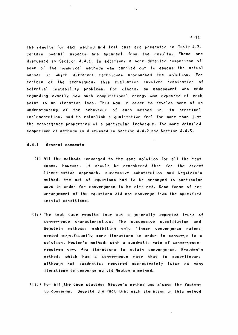
4.11

The results for each method and test case are presented in Table 4.3.

Certain overall aspects are apparent from the results. These are

discussed in Section 4.4.1. In addition, a more detailed comparison of

some of the numerical methods was carried out to assess the actual

manner in which different techniques approached the solution. For

certain of the techniques, this evaluation involved examination of

potential instability problems. For others, an assessment was made

regarding exactly how much computational energy was expended at each

point in an iteration loop. This was in order to develop more of an

understanding of the behaviour of each method in its practical

implementation, and to establish a qualitative feel for more than just

the convergence properties of a particular technique. The more detailed

comparison of methods is discussed in Section 4.4.2 and Section 4.4.3.

4.4.1 General comments

( i) All the methods converged to the same solution for all the test

cases. However, it should be remembered that for the direct

linearisation approach, successive substitution and Wegstein's

method, the set of equations had to be arranged in particular

ways in order for convergence to be attained. Some forms of re

arrangement of the equations did not converge from the specified

initial conditions.

(ii) The test case results bear out a generally expected trend of

convergence characteristics. The successive substitution and

Wegstein methods, exhibiting only linear convergence rates, l

needed significantly more iterations in order to converge to a

solution. Newton's method, with a quadratic rate of convergence,

requires very few iterations to attain convergence. Broyden's

method, which has a convergence rate that is superlinear,

although not quadratic, required approximately twice as many

iterations to converge as did Newton's method.

(iii) For all .the case studies, Newton's method was always the fastest

to converge. Despite the fact that each iteration in this method

4.12

METHOD

Direct Successive Wesstein's Newton's Broyden's Li near i sat ion Substitution Method Method Method

Its. Time Its. Time Its. Time Its. Time Its. Time

CASE 1 Single 16 12.9 108 41.8 133 54.1 4 5.5 5 7.0 Reactor

CASE 2 Selector 16 24.8 256 143.5 258 175.5 4 12.2 10 32.0 Reactor

CASE 3 Contact 12 18.3 619 347.0 576 391.4 4 12.2 8 25.5

Stabilisation

CASE 4 Five - in - 14 62.6 1663 2945.2 1605 3004.9 3 36.4 7 49.6

Series

CASE 5 UCT 10 25.1 606 501.5 615 605.4 4 24.1 8 49.2

Process

where Its. = number of iterations Time = time in seconds

Table 4.3 Test case results.

4.13

involves a complete re-computation of the Jacobian matrix, the

computational time expended per iteration is not excessive. In

addition, the case studies verify the advanta9e of the quadratic

conver9ence rate, as Newton's method requires si9nificantly fewer

iterations than any of the other methods to reach a solution.

This seems to be irrespective of the complexity of the

confi9urations, as the method consistently required only three or

four iterations to conver9e.

(iv) Broyden's method 9enerally required approximately twice the

number of iterations as Newton's method. This is in agreement

with the 9eneral conver9ence characteristics of quasi-Newton

methods i.e. those usin9 an approximation to the Jacobian matrix.

However, the ti me taken to reach conver9e-nce by the two methods

should then be approximately equal, 9iven that Broyden's method

requires only half the number of function evaluations to estimate

the Jacobian. Examination of Table 4.3 shows that, in practice,

this does not occur. In fact, Broyden's method consistently

required lon9er than Newton's method to converge. This aspect is

discussed in more detail in Section 4.4.3.

(v) Both the methods of 1Je9stein and successive substitution were

found to perform consistently poorly for all the test cases. This

was not entirely unexpected. The fact that both are simple to

implement and require very 1 ittle computational effort per

iteration is counterbalanced by inferior rates of conver9ence.

(vi) Successive substitution and 1Je9stein's method may appear to

perform disproportionately poorly for the five-in-series reactor

confi9uration of Case 4. On consideration, however, this result

is to be expected. Both these methods involve fixed point

iteration in which each state variable is modified without regard

for the simultaneous changes in other variables at each

iteration.

for this

Jacobian.

In contrast,

"simultaneity"

Therefore, when

Newton's method, for example, accounts

via the partial derivatives in the

successive substitution or 1Je9stein's

4.14

method is applied to a long train of reactors with no internal

recycles such as Case 4, inaccuracies in the initial estimates

"work through" the system slowly. The performance of these

methods is improved relatively when internal recycles are

included in the configuration as in Case 5 for example. These

recycle links in effect partially account for the interaction

between the state variables which is not directly considered with

successive substitution or Wegstein's method,

To explain this, consider a certain compound in a two reactor

system where the respective concentrations are denoted by x1 and

x2, If there is no recycle from reactor 2 to reactor 1, then the

mass balance equation for x1 does not contain the variable x2. As

a result, in the fixed point iteration step for x1 the influence

of the variable x2 is disregarded. In contrast, if there is a

recycle from reactor 2 to 1, then the variable x2 is incorporated

in the mass balance equation for x1. In this case, cognisance is

given to x2 when iterating for Xt.

(vii) The performance of Wegstein's acceleration method compared to

that of successive substitution was surprisingly poor. The lack

of improvement over successive substitution indicates that

Wegstein's method is not an appropriate acceleration technique

for these types of functions. A more detailed examination of the

relative merits of successive substituion and Wegstein's method

is presented in Section 4.4.2.

(viii) The direct linearisation method produced very favourable results1

for all the test cases. Accurate solutions were achieved, and

convergence was both rapid and efficient. In fact, for Case 4,

its performance is almost comparable to that of Newton's method.

The efficiency of the method also seems to be relatively

independent of the complexity of the system configuration and

operating conditions. In fact, fewer iterations and computational

effort were required to reach a solution in Case 5 - the most

complex configuration than in Case 1 the simplest case

study. The reason for the success of the direct linearisation

4 .15

method is that the functions for the biolo9ical system under

consideration are not particularly non-linear in the re9ions of

interest, and thus the linearised functions 9ive a 900d

approximation to the non-linear equations. However, as noted

earlier, a severe drawback of the method is the prior skill and

mathematical man i pu lat ion that are necessary before the method

can be implemented.

4.4.2 Comparison of the Wegstein and successive substitution methods

These two numerical methods both reached convergence for all situations,

al though in Case 4 many iterations were required before the tolerance

was eventually satisfied. The amount of computational time expended per

iteration for both techniques is near equal, althou9h 1Je9stein's method

generally takes sli9htly longer than successive substitution for each

loop. This is to be expected, as the methods are identical except for

the relatively inexpensive additional calculation of acceleration

factors and checks on these that are introduced with 1Je9stein's method.

The number of iterations required by each method in order to attain

convergence was found to be near equal, although 1Je9stein's method

consistently required a few more iterations than did successive

substitution, This is contrary to what was expected, as IJegstein's

method was ori9inally implemented to accelerate the rate of conver9ence

of successive substitution. This result demanded further investigation.

To examine the phenomenon more fully, various modifications of Case

Study 1 were considered. In one of these modifications, the sludge age

was changed to 30 days instead of 3 days Ca 11 other parameters were

maintained as before) and both methods were re-tested. Fi9ure 4.2 shows

the trend observed in the sum of the squares of the function values,

which was used as the stopping criterion for both methods. As expected,

IJegstein's acceleration method moves to the re9ion of solution more

rapidly than d~es successive substitution. IJhat is surprising, however,

is that ultimately IJegstein's method requires more iterations to reduce

4 .16

the error to within the specified tolerance. On closer examinaiton it

was apparent that the reason for this behaviour was a slight instability

introduced by We9stein's method. This is not readily noticable in the

plot of Fig 4.2.

Figure 4.3 shows the path followed by the concentration of particulate

biomass, Xa, in approachin9 the solution for Case Study 1. A9ain, with

We9stein's method, the value of Xa initially converges more rapidly to

the solution, with less overshoot, as would be expected. However,

althou9h the 9eneral trend introduced by the acceleration is towards a

more "damped" path, the individual points on the curve have more of a

tendency to osc i 11 ate than those 9enerated by the successive

substitution technique. When the solution is approached, this

instability prevents the convergence criterion from bein9 satisfied.

It appears from the results that there would perhaps be some merit in

using the approach suggested by Westerber9 et al (1979): that is,

applyin9 Wegstein's method at intervals. This would presumably

accelerate the successive substitution whilst avoidin9 the instabilities

associated with Wegstein's method.

4.4.3 Coaparison of Broyden's and Newton's methods

The relative convergence rates of these two methods bear out the

expected trends! Broyden' s method does not conver9e as rapidly or as

efficiently as Newton's method. However, the fact that Broyden's method

is so computationally expensive merits further investi9ation.

Case Study 2 was used to examine the details of how the computational

ener9y for each iteration in the methods was distributed. Table 4.4

shows this "division of effort" for the second, third and fourth

iterations. Both techniques took approximately three seconds to complete

each iteration. The major components are: (i) the time required to set

up the Jacobian (or its approximation) and (ii) the time required to

solve the resulting set of linear equations.

4 .17

100

90

80

70

- 60 NI> < -g ~c

50 E~ :, 0

SUCCESSIVE SUBSTITUTION

Vlt 40

30

20

10

0 1 2 3 4 5 6 7 8 9 10 11 12 13 14 15 16 17

Iteration Number

Fi9ure 4.2 Comparison of Wegstein and successive substitution methods

for Case Study 1 <Sludge age= 30 days)

1.45

1.44

1.43

1.42

1 .41

1.4 -ID 1.39 "'C

C ..00 1.38 x"' ::,

0

t 1.37

1.36

1 .35

1.34

1 .33

1.32

1.31

WEGSTEIN

0 20

SOLUTION

40

Iteration Number

60 80

Fi9ure ,4.3 Coapariaon of Xe values for We9stein and aucceasive

substitution aethods for Case Study 1.

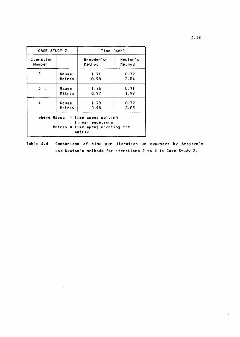
4 .18

CASE STUDY 2 Time (sec)

Iteration Number

2

3

4

where

Table 4.4

Broyden's Newton's Method Method

Gauss 1. 71 0.72 Matrix 0.98 2.04

Gauss 1. 76 0.71 Matrix 0.99 1.98

Gauss 1. 70 0.72 Matrix 0.98 2.03

Gauss = time spent solving linear equations

Matrix = time spent updating the matrix

Comparison of time per iteration as expended by Broyden's

and Newton's methods for iterations 2 to 4 in Case Study 2.

4 .19

Ci) Previous discussion has indicated that the major advantage of

Broyden's method is that, to set up the Jacobian approximation, it

requires fewer function evaluations at each iteration than Newton's

method, and thus should require less time per iteration. An

examination of the results in Table 4.4 shows that the time spent

by Broyden's method in updating the approximation to the Jacobian

is _roughly half that spent by Newton's method in re-evaluating the

complete matrix of partial derivatives (0.98 secs versus 2.02

secs>. This is to be expected as half the number of function

evaluations are required when using Broyden's method.

(ii) The major expense in Broyden's method is the disproportionate time

spent in solving the resulting system of linear equations by the

Gauss elimination procedure used here. In Broyden' s method, the

Gauss elimination takes more than twice as long to implement as it

does in Newton's method (1.72 secs versus 0.72 secs). The reason

for this is that sma 11 non-zero terms are introduced into the

matrix by Broyden's updating formula in locations that would

usually contain zeroes in the Jacobian. This effectively reduces

the sparsity of the Broyden matrix and severely hampers the

operation of the Gaussian technique, which relies on pivotal

rearrangement for its efficiency.

From the results above, it is apparent that, if the saving in the number

of function evaluations in Broyden's method is to be exploited, then

attention should be paid to the method used to solve the linear

equations. Perhaps this could be imp roved by us i n9 some specialised

matrix technique, rather than the Gaussian elimination used here.

4.5 GENERAL CONCLUSIONS

Ci) The method of direct linearisation, although performing

relatively efficiently for these test cases, is not a suitable

technique for general use in a simulation program. Thus, although

the preliminary analysis seems to have paid off in the

satisfactory performance of the method, the requirements of the

4.20

pro9ram that it be as 9enerally applicable as possible eliminates

direct linearisation from the possibilities that can seriously be

considered.

(ii) The methods of We9stein and successive substitution, althou9h

simple and robust, are inappropriate due to their slow rates of

conver9ence. Instability problems may be encountered in their

implementation and, as a result, conver9ence cannot always be

9uaranteed.

(iii) The poor performance of We9stein's method in comparison to that of

successive substitution could perhaps be eliminated by applyin9

We9stein only at selected intervals, as su99ested by Westerber9 et

al (1979>.

(iv) Broyden's method conver9es to a solution in comparatively few

iterations. The computational effort required to set up the

Jacobian approximation is rou9hly half that required by Newton's

method in settin9 up the true Jacobian. However, the method as

implemented here requires an excessive amount

effort per iteration, The major portion of'

concentrated in the solution of the system of'

Perhaps this bottleneck could be removed

specialised sparse matrix technique.

of' computational

this effort is

linear equations.

by employin9 a

(v) Of all the methods evaluated, Newton's appears to be the most

favourable. In addition, the use of' a finite difference

approximation to the Jacobian matrix renders it a 9enerally

suitable technique for the biolo9ical f'lowsheetin9 systems under

consideration.

CHAPTER FIVE

MODELLING OF THE DYNAMIC CASE

5.1 INTRODUCTION

In practice, the inputs to a biological system are unlikely to remain

constant. Because the influent to the system varies with time, the mass

balance equations describing the response of the system will take the

form of a set of differential equations incorporating time-dependent

terms [see Eqs (2.14) to (2.21), for example). This set of equations

wi 11 define how the values of the concentrations of each compound in

each reactor (the state variables) vary with time.

Solving the set of simultaneous differential equations is an initial

value problem. The magnitudes of the concentrations of each compound in

each reactor are specified as the initial condition, and thereafter the

equations are solved by integrating forward in time. In this way, the

changes in concentration in each reactor can be tracked, subject to the

variations in the influent flow rate and concentrations. In certain

circumstances, such as an activated sludge system, the influent pattern

of flow rate and concentration is repeated closely from day to day i.e.

a daily cyclic basis, A useful facility, therefore, is to predict the

steady state cyclic response when it is assumed that the influent

pattern is repeated identically from day to day. To find this solution

will require integrating forward through perhaps many cycles until

convergence to the solution is attained. Convergence in this case

requires that the cyclic concentration response of each compound in each

reactor is identical from cycle to cycle, and the values at the start

and end of each cycle are the same.

The set of differential equations describing the response of a

biological system under dynamic conditions will contain non-linear

terms, as did the mass balances for the steady state case. The task of

finding the solution to a such a set of non-linear ordinary differential

equations is certainly not unique to biological systems, Many systems of

5.2

interest to engineers and scientists are described by non-linear

differential equations. A multitude of numerical integration techniques

exist for the solution of these sets of equations. Consequently, when

faced with such a set of equations, the problem in finding a numerical

method is the selection of an appropriate one from the many diverse

methods available.

In the selection of an integration technique for the dynamic problem,

the approach taken was to initially establish a rudimentary integration

module which could be gradually refined and improved. In the process of

refining the module, a greater understanding of the actual dynamics of

the system was generated. This in turn indicated further adjustments

that could be made to the routine to improve it still further. Thus,

through an interactive process, the integration routine was gradually

tailored to better meet the demands of the biological system under

consideration. In the interests of clarity, this presentation will

follow the manner in which the actual integration module was developed

and incorporated in a dynamic simulation computer program. Each of the

series of refinements will be presented and discussed in the same

sequence as incorporated into the program.

5.2 USING NUMERICAL INTEGRATION TECHNIQUES

Because the exact solution to the set of differential equations is not,

in general, known and cannot be calculated analytically a numerical

integration technique will be required to provide an approximation to

the solution. One common approach, which will be the focus of this

presentation, is to use a time-stepping or difference method which

approximates the solution by its value at a sequence of discrete points

called the mesh points. Given a differential equation y' (x) = 0, a

difference method provides some rule for approximating y at a point xn

(y(xn)) in terms of the value of y at xn-1 and possibly at preceding

points. Ideally, the solution should be represented by its actual value

at each mesh point so that it can be approximated to high accuracy by

interpolatio'"!, between the mesh points. However, the exact solution to

the differential equation is not known, so it is always an approximation

5.3

that is sought. Many techniques assume that the mesh points are equally

spaced. However, since the step size seems to have an effect on the

error introduced, it is usually possible to vary the mesh spacing to

account for th is. For the moment, it wi 11 be assumed that the mesh

spacing remains constant during the stepping procedure. However,

variable step size integration procedures will be examined in more

detail ,later.

s.2.1 A siaple Euler aethod

The simplest stepping technique available is Euler's rule. This was used

as the first attempt to solve the set of differential equations

generated by the biological model. In the Euler method, the value of the

dependent variable at one point is calculated by straight line

extrapolation from the previous point. Generally referred to as a one

step method, Euler's rule is an algorithm which prescribes the numerical

technique for calculating the approximation to the solution at xn+1 in

terms of the value at one previous step, Xn. Consider the function Y

with

dy y' (x) = = f(x,y)

dx ( 5.1)

The value of y at Xn+l = <xn + h) may be approximated by a Taylor's

expansion. Truncating after the first two terms in the series yields:

Y ( Xn +h) ~ Y ( Xn ) + h • f ( Xn I Y ( Xn ) ) (5.2)

where h = steplength

The error in this approximation is described by the remaining terms in

the Taylor's expansion:

h2 h3

- . y I I ( Xn ) + - . y I I I ( Xn ) + •••• 2! 3!

(5.3)

5.4

and is called the local truncation error. A more detailed discussion

about the errors introduced by a stepping method, and the resultant

implications will be covered in Section 5.3.

Euler's rule is usually formulated as:

Yn + t - Yn + h · f n (5.4)

and in this form can be described as an explicit linear one step method

of first order.

5.2.1.1 An illustrative example

Dahlquist and Bjorck (1974) provide an example to illustrate the use of

Euler's formula for a single differential equation:

dy = y

dx with y(O} = 1

Euler's rule gives the following:

Yn + t = Yn + h · Yn Yo = 1 (5.5}

Table 5.1 presents the results obtained by first computing the solution

with h = 0.2 and then with h = 0.1, and compares these with the exact

solution. An examination of the Table reveals that the error is

approximately proportional to the stepsize. In other words, if the error

in the integration is to be halved, then the stepsize will also need to

be halved. This implies that, to attain reasonable accuracy with Euler's

method, the stepsize chosen needs to be smal 1. This is an inherent

weakness in using a first order method.

5.2.2 Multistep aethods and predictor-corrector pairs

Multistep methods present a distinct advantage over one-step methods

such as the first order Euler's rule. These methods exhibit improved

5.5

Exact STEPSIZE

Solution h = 0.2 h = 0.1

Xn Y ( Xn ) Yn h · fn error Yn h · fn error

o.o 1.000 1.000 0.200 0.000 1.000 0.100 0.000

0 .1 1.105 1.100 1.110 -0.005

0.2 1.221 1.200 0.240 -0.021 1.210 0 .121 -0.011

0.3 1.350 1.331 0.133 -0.019

0.4 1.492 1.440 0.288 -0.052 1.464 0.146 -0.028

0.5 1.649 1.610 0.161 -0.039

0.6 1.822 1. 728 -0.094 1. 771 -0.051

Table 5.1 Euler's method executed with two different stepsizes

(Dahlquist and Bjorck, 1974)

accuracy and conver9ence characteristics, althou9h at the expense of

requirin'3 additional computation. Recall that Euler's method only

required the value at one mesh point to compute the value at the next.

Multi-step methods use more than one value of the dependent variable to

calculate the equivalent information at the next time interval. Recall

also that Euler's method was referred to as explicit; that is, Yn+t

occurs only on the left hand side of the equation and can be calculated

directly from the ri9ht hand side values. Linear multistep methods are

generally implicit; that is, the unknown value occurs on both sides of

the equation and cannot be calculated directly. These implicit methods

in general entail a substantially greater computational effort than do

explicit methods. On the other hand, implicit methods can be made more

accurate than explicit methods and enjoy more favourable stability

properties (Lambert, 1974). In fact, these considerations so favour

implicit methods that explicit linear multistep methods are seldom used

on their own.

The followin'3 formula, the second order trapezoidal method,

Yn + t - Yn h

= - · [ f ( Xn , Yn ) + f ( Xn + t , Yn + t ) ] 2

5.6

(5.6)

is an example of an implicit method, since Yn+t, which is to be

computed, appears implicitly on the right hand side. If f is a non

linear function, a non-linear system will need to be solved at each

step. This must be done by some iterative method, for example, by the

procedure:

h Yn + t = 2 · [ f ( Xn I Yn ) + f ( Xn + t I Yn + t ) ] + Yn (5.7)

To solve Eq (5.7), a reasonable initial estimate of Yn+t can be obtained

using past values of y with, for example, Euler's explicit formula. In

this context, the explicit formula is usually referred to as the

predictor, whilst the implicit formula of Eq (5.6) is referred to as the

corrector. Used in combination, these two equations make up a procedure

called a predictor-corrector method, Lapidus (1971) refers to a

predictor-corrector method that is used in this way as a PECE method,

indicating that a predicted value of Yn+t is followed by a derivative

evaluation , Y'n+t, and then Yn+t is corrected and y'n+t evaluated.

Termination of the integration step may be controlled in one of two

ways. The first consists of continuing the iterative scheme suggested by

Eq (5,7) until the iterates have converged. In practice, this would

usually involve comparing the difference between two successive

estimates of the solution to some preset tolerance. If the difference is

smaller than this tolerance, then the latest value of y obtained may be

regarded as an acceptable approximation to the exact solution of the

equation. Since each iteration corresponds to one application of the

corrector, this mode of operation of the predictor-corrector method is

referred to as correctin'3 to conver'3ence <Lambert, 1974). In this mode,

there is no way of telling in advance how many iterations will be

necessary and consequently how many function evaluations will be

required at each step.

5.7

The second approach for terminating the integration step is motivated by

the desire to restrict the number of function evaluations per step. The

number of times, m, that the corrector is applied at each step is

stipulated in advance. This approach is more common than the method of

correcting to convergence. This mode of operation can be described as a

PECCE)• method, where the predicted Yn+t and evaluated fn+t is followed

by m corrections and derivative evaluations,

Of the two approaches, Lapidus (1971) recommends the PECCE)• method with

m = 1 as being one of the most successful means to apply these

predictor-corrector formulae. Using only a single application of the

corrector formula saves on the number of function evaluations reQuired -

only two function evaluations are reQuired per iteration step.

5.3 ERROR CONTROL

Once a time-stepping method has been selected to carry out the numerical

integration procedure, the next stage is to evaluate the accuracy of the

so 1 ut ions that it generates. For each step of the difference procedure,

some form of approximation is used to obtain the next estimate of the

solution. Thus, each step taken will generate an associated error term,

This is a natural conseQuence of any approximation techniQue. Given that

this error can never be entirely eliminated, the best approach is to

ensure that it is continuously evaluated and maintained at acceptable

levels. In addition, the stepping procedure should be able to

incorporate adjustments to the relevant parameters as soon as the error

begins to accumulate. It is the nature of this cumulative error that

wi 11 be decisive in the eventual success or failure of each step of the

integration method.

5.3.1 Sources of error

In using a stepping or difference method to find the solution to a

differential eQuation, the solution that is eventually found will never

be exact. The difference between this solution and the exact solution is

5.8

the local error. Sources of error will

<Dahlquist and Bjorck, 1974)!

include, amongst others,

(i) The round-off error introduced by using finite precision numbers.

(ii) The truncation error associated with the linear multistep method

used. This is the error occurring when a limiting process is

truncated or broken off before the limiting value has been

reached.

Once the primary sources of error in a stepping method have been

identified, it is necessary to be able to use this information in such a

way as to ensure that all errors are minimised as far as possible. This

wi 11 involve an assessment of how each of the error terms affect the

reliability of the method, which sources of error dominate and how a

kn owl edge of the error can be used in maintaining the accuracy of the

stepping algorithm.

5.3.2 Estiaatins the local error

Dahlquist and Bjorck (1974) demonstrate that, for an integration method,

of order p the local error is approximately bounded by!

[

hj(p+ll ln::: cn·--

2

where ln = local error

p = order of the integration method

h = stepsize

Cn = a constant specific to the integration method

(5.8)

Dahlquist and Bjorck (1974) provide an alternative formulation for a

predictor-corrector method. They propose that the error of the predicted

value can be expressed by a difference function using a constant, c',

which is speci"fic to the order of the predictor. The difference between

5.9

the predicted and the corrected values, multiplied by c/(c'-c) is then

an estimate of the local error of the corrected value:

C • ( yp Ye) 1 .. = -

( C, - C) (5,9)

where C = a constant specific to the order of the predictor

CI = a constant specific to the order of the corrector

yp = predicted value of y

Ye = corrected value of y

5.3.3 Percentage accuracy

An error tolerance must be selected to satisfy the dual requirements of

reliability and efficiency. If a very strict tolerance is chosen,

unnecessary computational effort wi 11 be expended in order to meet its

requirements. If the tolerance chosen is not sufficiently strin9ent, it

is possible that the effect of a cumulative error wi 11 eventually lead

to instability of the method and jeopardise its chances of successful

conver9ence. In practise, it has been found convenient to express this

tolerance in terms of a "percenta9e accuracy" where this percenta9e

accuracy is defined in the same way as a relative error measurement.

That is:

Y<,-t> - Y<,> X ace= · 100

where

Y<, - t,

Y<,> = current estimate of the value of the variable

Y<,-t1 = previous estimate of the value of the variable

X ace= percentage accuracy

(5.10)

Definin9 the accuracy requirements in this way enables calculation of

error tolerances that are independent of the absolute ma9nitude of the

variables involved. Consequently, the accuracy specifications can be

transformed into numerical lan9ua9e that is equally si9nificant for

variables with very small or very lar9e ma9nitudes. This is an important

consideration, especially for badly scaled problems, such as those

encountered in biolo9ical systems. Practically, this is achieved with

5.10

the use of an error tolerance, E, which is defined in terms of the

percentage accuracy required and is the limiting value that the local

error may reach without jeopardising the success of the step. Once a

percentage accuracy is specified, this must be transformed into an E

value which applies to each variable. This can be achieved by firstly

reformulating Eq 5.10 to give:

X ace= yp - C ___ Y_ • 100

yp (5.11)

Given that, in the limiting situation,

E = l n (5.12)

a limiting value for E for each variable in a set of simultaneous

differential equations may be derived by combining Eqs. (5.9), (5.11)

and (5.12) as follows:

C . ( yp Ye ) E = -( C • - c)

C X ace· y, = (5.13)

( C, - C) 100

Equation (5.13) now provides a means of selecting an error tolerance for

each variable which is based on a percentage accuracy requirement but

which also incorporates a measure of the scale of the variable involved,

yP. Equation (5.13) is useful because it al lows the user to specify a

completely general percentage accuracy requirement for the integration

module. This specification is then used to calculate a separate E value

for each component in the sytem. This error tolerance can now be used as

the basis for estimating the next stepsize for each component.

5.4 STEPSIZE SELECTION

For any efficient difference method for integration, an objective is to

use integration steps that are as large as possible, whilst preserving

the required accuracy. Once an estimate has been made of the magnitude

5.11

of the error generated at an integration step, this estimate can be used

to decide whether or not the most recently computed value of the

variable is acceptable. If the error is found to be larger than a

predetermined tolerance, the value wi 11 be rejected and then recomputed

using a smaller stepsize. If the error is within the bounds prescribed,

then the value wi 11 be accepted and a larger step can be taken in order

to generate a new estimate.

Ideally, the size of each new steplength should be selected so that it

reflects the magnitude of the error in the previous calculation. In

other words, if the value falls well within the prescribed error bounds,

a large increase in the steplength should be permitted. If the error in

the value is close to the tolerance, then the subsequent steplength

should be allowed to increase, but not so dramatically. It is suggested

by Dahlquist and Bjorck (1974) that, in order to maintain the local

error below a given tolerance, the new stepsize should satisfy the

following condition:

[

h'](p+l) Cn. --

2 (5.14)

where h' = new stepsize

8 = a preset safety factor to account for the fact that the

error estimates are approximate and based on experience

from the preceeding interval (8 ~ 1)

From Eq (5.9):

[

hl(p+l)

ln ~ Cn • --

2

Therefore, eliminating Cn in

(5.15)

Eq (5.14) yields:

[ 1

1/(p+t)

S·E h' = h . --

1 n

5.12

(5.16)

The usefulness of this formulation to determine the subsequent stepsize

rests on the fact that it incorporates the absolute magnitude of the

error generated by the previous step. This means that the calculation of

the next stepsize is based on a quantitative assessment of exactly how

successful the previous step was.

5.5 DYNAMIC BEHAVIOUR OF BIOLOGICAL SYSTEMS

The preceding sections have dealt with the selection of integration

technique and step length adjustment in general terms. This information

is now implemented for the simulation of biological system behaviour

under dynamic conditions. The discussion is best introduced by

considering a numerical example.

Consider the behaviour observed in an aerated batch reactor into which

heterotrophic organisms <Xe) and a readily biodegradable soluble

substrate <Ss) are introduced at time t = O. Assume that the initial

concentrations are Xeo = 1000 g.m- 3 and Sso = 100 g.m- 3 respectively.

Assume also that the behaviour in the batch reactor is governed by the

model introduced earlier (Chapter 2, Table 2.2) and that the kinetic and

stoichiometric constants are those used in the case studies (Chapter 4,

Table 4.1). At the start of the batch test, the changes in concentration

of Xe and Ss will be dominated by the growth process. Organism decay

will exert only a minor influence on Xe. The rates of change of

concentration at t = D will be:

For Xe :

dXe Sso "' Xs o - b · Xeo = u·

dt 0 < Ks + Ss o >

100 1 ODO - D. 62 · 1000 = 4·

(5 + 100)

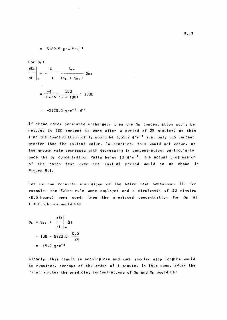
5 .13

= 3189.5 9 · m- 3 • d- 1

For Ss :

dSs " Ss o u = - --· Xa o

dt 0 y < Ks + Ss o >

-4 100 1000 = ---·-----

0.666 (5 + 100)

If' these rates persisted unchanged, then the Ss concentration would be

reduced by 100 percent to zero after a period of 25 minutes: at this

time the concentration of Xs would be 1055.7 g·m- 3 i.e. only 5.5 percent

greater than the initial value. In practice, this would not occur, as

the growth rate decreases with decreasing Ss concentration, particularly

once the Ss concentration falls below 10 g·m- 3• The actual progression

of the batch test over the initial period would be as shown in

Figure 5.1.

Let us now consider simulation of the batch test behaviour. If, for

example, the Euler rule were employed and a steplen9th of 30 minutes

(0.5 hours) were used, then the predicted concentration for Ss at

t = 0.5 hours would be:

dSs Ss = Ss o + lH

dt 0

0.5 = 100 - 5720.0·

24

= -19.2 9· m- 3

Clearly, this result is meaningless and much shorter step lengths would

be required, perhaps of the order of' 1 minute. In this case, after the

f'irst minute, the predicted concentrations of Ss and Xs would be!

1.1

1

0.9

0.8

0.7

] 0.6 :t: C

c3 0.5 d 0.4

0.3

0.2

0.1

0 0

Fi9ure 5.1

2 4

.

6

Xb

8

Time

5 .14

Ss

10 12 14

The progression of a batch test showing the response of Ss

and X1.

5.15

Ss 100 + (- 5720.0) 1/60

= 24

= 96. 0 g · m- 3 < i • e. a change of 4 percent)

Xe = 1000 + 1/60

3189.5 24

= 1002.2 < i • e. a change of 0.22 percent)

Given that the percentage change of Xs is only one twentieth that of Sa

over the interval, it appears that the step length of 1 minute is

unnecessarily short to track the changes in Xs with acceptable accuracy.

However, because the variables Xs and Ss are coupled, the two equations

should strictly be integrated simultaneously. This implies that the step

length used for the integration procedure will be limited by the maximum

allowable size for the rapidly changing Ss, and Xs will be tracked with

"unnecessary" accuracy.

Gear (1984) noted that behaviour similar to the reponse in the batch

test is encountered in many engineering systems. Although strictly these

variables are coupled, he suggested that the degree of coupling between

the variables might not be strong. Gear proposed that, if this is so,

then the differential equations for each of the variables may be

integrated separately. In the batch reactor examp 1 e, Gear's approach

would mean that longer step lengths could be used for integrating Xs

than those required for Ss. This offers the advantage of increased

computational efficiency without compromising on accuracy requirements.

Implementing Gear's multirate approach involves partitioning a system of

equations into different groups, each of which is governed by different

dynamics. A group governed by "fast" dynamics would require short

integration steps, whereas a group exhibiting "slow" dynamics could be

integrated using longer integration steps. Gear proposed a number of

schemes to account for the coupling between components with "fast" and

"slow" dynamics.

5.16

5.6 THE USE OF A HULTIRATE TECHNIQUE

5.6.1 Methods for handlin9 the coupled equations

Consider a two component system Cone fast, one slow) which is described

by two coupled ordinary differential equations. Assume that this system

is inte9rated from to to (to + LH> using a stepsize h for the "fast"

component and H for the "slow" component, where H > h and H = rh. This

division is shown in Fig 5.2.

h

to

Fi9ure 5.2

H--------------.....i

( to +h) Cto+2h) (to+Cr-1)h) C to +H >

Schematic representation of small and large timesteps for a

multirate integration technique

At any point in the integration process, values of both the "slow" and

the "fast" variables will be required in order to complete the next

integration step. At ( to +h), the next integration step for the "fast"

component to Cto+2h) wi 11 require a knowledge of the value of the "slow"

compound at least at Cto+h). If the "slow" compound is integrated first,

then its most recently computed value will be that at the end of the

long time interval, to+H. If the "slow" compound has not yet been

integrated, then the latest available value will be that at to, the

beginning of the large time interval. In either case, an explicit

estimate of the value of the "slow" compound at Cto+h) is not available.

The same problem will be encounterd at Cto+2h), Cto+3h), ... etc.

Estimation of the value of the "slow" compound at these intermediate

points (to+h, to+2h, ••• .to+Cr-1>h) is the crux of the problem of

simultaneous multirate integration.

5.17

Two approaches to solvin'3 the problem have been su'3'3ested. The first

approach ("fastest first") inte'3rates the "fast" compounds over (r-1)

steps of size h and then simultaneously inte'3rates the "fast" and "slow"

components to advance them to the end of the interval usin'3 stepsizes h

and H respectively. For the small inte'3ration steps, values of the

"slow" component are obtained by extrapolation from previous values

(i.e. at to and before) with a predictor-like formula. Gear (1984) notes

that the error incorporated into the method throu'3h this extrapolation

should be "of tolerable size". The disadvanta'3e of this "fastest first"

approach, however, is the amount of stora'3e space consumed by the

necessity to back up the "slow" variables in case of an inte'3ration step

failure. If a step fails and the "slow" variables have not been stored,

then they will need to be recalculated. The effort involved in

accomplishin'3 this task is an additional drawback to the "fastest first"

approach.

The second approach ("slowest first"), which has been recommended by

Gear (1984) and is adopted in this study, involves inte'3ratin'3 the

"slow" compounds to the end of the lar'3e timestep first. Interpolation

techniques are then used to obtain intermediate values for the "slow"

compounds at the points Cto+h), Cto+2h), ••• ,Cto+Cr-1)h). This then

allows inte'3ration of the "fast" compounds in short steps from to to

(to + H). IJith this approach, the extrapolation of the "fast" variables

to inte'3rate the "slow" variables first will lead to lar'3e errors in the

extrapolated values because the extrapolation is over many timesteps in

the "fast" variables. Gear maintains that this is miti'3ated by the fact

that couplin'3 from the "fast" values to the "slow" values is '3enerally

small. This, in fact, is the basis for the method. An important

advanta'3e of the "slowest first" method is that, if a variable has to be

backed up because of an inte'3ration failure in another variable, the

backup is simply a reduction of the size of the last step taken, and can

be done provided that only one additional value is kept for all

variables.

5.18

5.6.2 Partitioning of a system

Partitioning a system into cate9ories havin9 different dynamics is an

important consideration in the use of a multirate technique. Various

methods for automatic partitionin9 of the system have been investi9ated

(Gear, 1984: Ora i 91091 u, 1983). These methods have been found difficult

to implement and expensive in terms of computational time. Therefore,

static partitioning, where the division into categories is specified by

the user prior to the inte9ration, is 9enerally applied.

A problem that arises in partitionin9 is what exactly defines dynamics

as "fast" or "slow"? One possible answer is that "fast" components

exhibit a large differential term i.e. (dC/dt) is lar9e. Another

possible solution would be that it is a rapidly chan9in9 (dC/dt) term

that indicates "fast" dynamics. Alternatively, perhaps the ratio

(dC/dt)/C is an appropriate measure for reaction systems where the

concentration C cannot decrease to less than zero. The question does not

appear to have been resolved in the literature and decisions as to the

classification of compounds are usually based on practical experience

and knowled9e of the physical system.

5.6.3 Integration errors with a multirate technique

In choosin9 a time-steppin9 al9orithm for the solution of the dynamic

problem, the question of error estimation and control is a central one.

Decisions as to whether or not concentration variables are acceptable

have to be based on some estimation of how close these are to the actual

solution. In usin9 a multirate technique to carry out the integration

procedure, the con tr i but ion to the 91 oba l error in the method may stem

from a number of sources. For the "slowest first" technique, the sources

of error include the round off error and the local truncation error as

described in Section 5.3.1 as well as:

( i) The error associated with the extrapolation of the "fast"

components to allow inte9ration of the "slow" components even .

thou9h the fast components have yet to be inte9rated.

5.19

(ii) The error associated with the interpolation of the slower

components to allow integration of the "fast" components. The

interpolation error depends on the method used, and is due to two

effects: firstly, the errors in the interpolation formula itself

and secondly, errors due to errors in the mesh values. Gear (1984)

notes that the errors in the interpolation formula will be

significantly less than those in an extrapolation formula over the

same interval.

In controlling the error, Gear (1984) suggests ensuring that the

contributions from the interpolation and extrapolation are small in

comparison to the local truncation error term. The local error term can

then be used to select the next stepsize on the basis of a given error

tolerance. An error tolerance term, E, can be calculated for each

component in each of the "fast" and "slow" groups. Once all the E values

for al 1 the components have been computed, the largest E value for each

group is chosen as the limiting value. It is this limiting E that will

determine the size of the subseQuent integration step for all the

components in that group.

5.6.4 Stepsize selection with a aultirate technique

The concept of using a mult irate method is to reduce computation in an

integration problem by using different stepsizes for groups of

components with differing dynamics. Efficiency can be increased further

by using the longest possible stepsize within each group.

Gear (1984) recommends an incremental approach for integration

steplength adjustment that was used in the early stages of the

development of the integration module here. Very simply, if the error in

any component in either the "fast" or "slow" group is greater than the

prescribed tolerance, then the value is rejected and the next steplength

for that group will be half the size of the previous one. If the error

is less than the prescribed tolerance, then doubling of the next

5.20

steplength is permitted. These stepsize changes are subject to certain

constraints and may only take place at particular points in the

integration scheme. This is possibly the most simple approach that can

be taken in formulating some kind of dynamic relationship between error

magnitude and stepsize control. One of its major limitations is that it

makes no distinction between solution estimates that fall well within

the prescribed error bounds and those that only just satisfy the error

criterion. This is a significant limitation because the stability

behaviour of the system is detrimentally affected by the accumulation of

errors in the calculated variables.

A possible approach to overcome the 1 imitations of Gear's method for

steplength adjustment, would be to use the variable steplength

adjustment method of Dahlquist and Bjorck (1974) (See Section 5.4). This

is justified because the local error term is dominant.

5.7 IMPLEMENTATION OF GEAR'S MULTIRATE TECHNIQUE

The basis for developing and evaluating the multirate integration

technique was a continuation of the case study first introduced in

Section 2.5; that is, the single reactor plus settling tank problem

based on the limited IAIJPRC model (Table 2.2). Equations (2.14) to

(2.21) are the set of differential equations and algebraic equations

describing the sytem. Numerical values for the problem (reactor volumes,

kinetic constants, etc) were the same as those used for Case Study 1 in

Chapter 4 <Tables 4.1 and 4.2).

To introduce the dynamic component, a square wave cyclic input pattern

was imposed on the system. In this scheme, the fu 11 vo 1 ume of feed for

Case Study 1 in Chapter 4 was introduced into the reactor at a constant

rate but over a twelve hour period in a twenty four hour cycle. For the

remaining twelve hours of the cycle, there was no feed. That is, the

system was subjected to a step increase in flow rate and twelve hours

later to a step decrease to zero flow. This input pattern was selected

because, in the region of the step changes, it would provide a rigorous .

test of the integration method.

5.21

There are two requirements before a multirate integration technique can

be initiated:

(i) For an initial value problem such as this, a set of values for each

of the state variables at time t = 0 is required to initiate the

integration. In this case, the simulation program uses the set of

state variables which constitute the solution to the steady state

problem as initial values for the dynamic case.

(ii) Implementing a multirate technique involves partitioning the

compounds into categories with either "fast" or "slow" dynamics.

The model incorporates four compounds: three particulate compounds

(Xe, XE and Xs> and one soluble compound (Ss). After investigating

the nature of the dynamics of each of these compounds, it was

decided to classify Xs and XE as "slow" and Ss as "fast".

In the case of Xs, it was found by trial that the dynamics are

neither as "fast" as those of the soluble compound nor as "slow" as

those of the particulate compounds. In fact, it appears that, in

certain circumstances, the behaviour of Xs changes from "fast" to

"slow". Classifying the dynamics of Xs as "slow" and using long

time steps for its intergration may result in inaccuracies in the

solution. On the other hand, categorising it with the "fast"

compounds in the system could result in needless extra

computational effort as a result of the unnecessarily small

timesteps being used at times when Xs exhibits "slow" dynamics. As

a result, there seemed to be the potential to incorporate this

compound into some kind of intermediate category. Creating an

additional category for "intermediate" dynamics would thus have the

advantage of enabling the routine to cater specifically for this

compound and select an exactly appropriate stepsize for its

integration. One drawback of this approach, however, would be the

extra programming code required to extend the number of categories

from two to three. If the whole purpose of a multirate technique is

to improve efficiency, then the added complexity of accounting for

5.7.1

5.22

the coupling between three groups of variables would perhaps negate

this objective at the outset. On the other hand, the ultimate

efficiency of the technique depends on the appropriate partitioning

of the system. In viewing these alternatives, it was decided to

maintain the simpler approach and restrict the number of divisions

to two. The effect of partitioning Xs with either the "fast" or the

"slow" group is discussed in Section 5.9.1.

The initial multirate scheme

Gear (1984) has recommended that as many of the parameters as possible

in a modern program code should be selected automatically. Achievin9

this for an integration scheme does present some difficulties

particularly when implementing a multirate technique. This is due to the

large number of parameter choices involved. As a result, the initial

approach to the problem relied on prior specification of a number of the

variables in accordance with the suggestions of Gear (1984)!

(i) The initial stepsize for the "slow" components, H, was set at an

arbitrary value to initiate the inte9ration.

(ii) The ratio of the number of sma 11 steps to the number of 1 ar9e

steps was also specified and remained fixed throughout the

integration.

(iii) Initially, the steplengths could only be increased or decreased by

a factor of two.

The "slowest first" technique recommended by Gear (1984) was followed. A

simple Euler formula was used for both the "slow" and the "fast"

integrations.

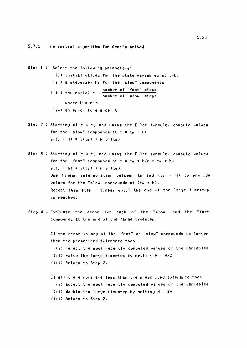
5.23

5.7.1 The initial alsorithm for Gear's method

Step 1 Select the followinS parameters:

( i ) initial values for the state variables at t=O. ( i i ) a stepsize, H, for the "slow" components

number of "fast" steps ( i i i ) the ratio! r =

number of "slow" steps

where H = r · h

( i V) an error tolerance, E

Step 2 : Start ins at t = to and us ins the Euler formula, compute values

for the "slow" compounds at t = to + H:

y ( to + H) = y ( to ) + H · y' ( to )

Step 3 : Start i n9 at t = to and using the Euler formula, compute values

for the "fast" compounds at t = to + H/r = to + h:

Step 4

y(to + h) = y(to) + h·y'(to)

Use linear interpolation between to and (to + H) to provide

values for the "slow" compounds at <to + h).

Repeat this step r times, until the end of the larse timestep

is reached.

Evaluate the error for each of the "slow" and the "fast"

compounds at the end of the large timestep.

If the error in any of the "fast" or "slow" compounds is larser

than the prescribed tolerance then

(i) reject the most recently computed values of the variables

(ii) halve the large timestep by setting H = H/2

(iii) Return to Step 2.

If all the errors are less than the prescribed tolerance then

(i) accept the most recently computed values of the variables

(ii) double the large timestep by setting H = 2H

(iii) Return to Step 2.

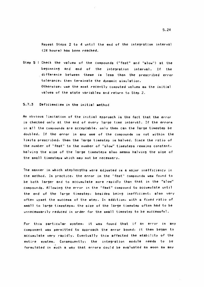
5.24

Repeat Steps 2 to 4 until the end of the integration interval

(24 hours) has been reached.

Step 5: Check the values of the compounds ("fast" and "slow") at the

5.7.3

beginning

difference

and end

between

of

these

the

is

integration

less than

interval. If

the prescribed

tolerance, then terminate the dynamic simulation.

the

error

Otherwise, use the most recently computed values as the initial

values of the state variables and return to Step 2.

Deficiencies in the initial aethod

An obvious limitation of the initial approach is the fact that the error

is checked only at the end of every large time interval. If the errors

in all the compounds are acceptable, only then can the large timestep be

doubled. If the error in any one of the compounds is not within the

limits prescribed, then the large timestep is halved. Since the ratio of

the number of "fast" to the number of "slow" timesteps remains constant,

halving the size of the large timesteps also means halving the size of

the small timesteps which may not be necessary.

The manner in which steplengths were adjusted is a major inefficiency in

the method. In practice, the error in the "fast" compounds was found to

be both larger and to accumulate more rapidly than that in the "slow"

compounds. Allowing the error in the "fast" compound to accumulate until

the end of the large timestep, besides being inefficient, also very

often upset the success of the step. In addition, with a fixed ratio of

small to large timesteps, the size of the large timestep often had to be

unnecessarily reduced in order for the small timestep to be successful.

For this particular system, it was found that if an error in any

component was permitted to approach the error bound, it then began to

accumulate very rapidly. Eventually this affected the stability of the

entire system. Consequently, the inte43ration module needs to be

formulated in such a way that errors could be evaluated as soon as any

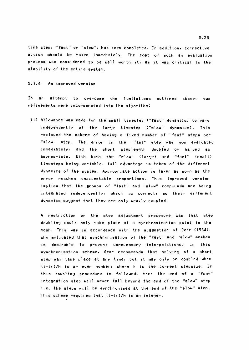
5.25

time step, "fast" or "slow", had been completed. In addition, corrective

action should be taken immediately. The cost of' such an evaluation

process was considered to be we 11 worth it, as it was er it i cal to the

stability of' the entire system.

5.7.4 An improved version

In an attempt to overcome the limitations outlined above, two

refinements were incorporated into the algorithm:

Ci) Allowance was made for the small timestep ("fast" dynamics) to vary

independently of' the large timestep ("slow" dynamics>. This

replaced the scheme of' having a fixed number of' "fast" steps per

"slow" step. The error in the "fast" step was now evaluated

immediately, and the short steplength doubled or halved as

appropriate. With both the "slow" (large) and "fast" (small)

timesteps being variable, full advantage is taken of' the different

dynamics of' the system. Appropriate action is taken as soon as the

error reaches unacceptable proportions. This improved version

implies that the groups of' "fast" and "slow" compounds are being

integrated independently, which is correct, as their different

dynamics suggest that they are only weakly coupled.

A restriction on the step adjustment procedure was that step

doubling could only take place at a synchronisation point in the

mesh. This was in accordance with the suggestion of' Gear (1984),

who motivated that synchronisation of' the "fast" and "slow" meshes

is desirable to prevent unnecessary interpolations. In this

synchronisation scheme, Gear recommends that halving of' a short

step may take place at any time, but it may only be doubled when

(t-to )/h is an even number, where h is the current stepsize. If'

this doubling procedure is followed, then the end of' a "fast"

integration step will never fall beyond the end of' the "slow" step

i.e. the steps wi 11 be synchronised at the end of' the "slow" step.

This scheme requires that (t-to)/h is an integer.

5.26

(ii} The simple Euler rule was replaced by a predictor-corrector pair.

The Euler formula was retained as the predictor, and the second

order trapezoidal rule was used as the corrector. With this

approach, the number of function evaluations would be doubled at

each integration step. However, it was hoped that the more

sophisticated integration technique would allow more than a

doubl ins of the step lengths, thus giving an overall increase in

efficiency. The single application of the corrector was in line

with the recommendation of Lapidus (1971}.

5.7.4.1 Deficiencies in the improved method

Two problems were apparent with the improved scheme:

(i} With both timesteps being variable, synchronisation of the meshes

is more difficult.

(ii} Computational effort can be wasted if the size of the error in the

large timestep is not within acceptable limits and the step fails.

The error in the "slow" compounds is only checked at the end of

every large interval, which means that the already completed

computation for the "fast" compounds is wasted if the large

timestep is unsuccessful.

5.7.5 Further iaprovements

To address the deficiencies outlined above, two additional modifications

were proposed:

(i) The first improvement in the integration method involved removing

the synchronisation constraint. Thus, doubling and halving of

"fast" and "slow" step lengths could take place at any point. In

the case of the

found that the

"fast" steps,

integration

if by doubl ins a "fast" step, it was

would move to beyond the end of the

current "slow" step, then a smaller step would be taken to arrive

exactly af the end of the "slow" step i.e. truncatin9 to ensure

5.27

synchronisation. At the start of the next "slow" integration step,

the new "fast" step length would be based on the step length

calculated prior to truncation. This ensured relatively unlimited

adjustment of the "fast" step lengths within the "slow" steps. In

the case of the "slow" steps, truncation was only required where a

"slow" step beyond a data storage point was attempted. In the new

scheme, the "slow" step was truncated in a similar manner as for

the "fast" step, to end at the data storage point.

(ii) ~ith the improved method, the problem of computational effort

"wasted" on the "fast" steps when the "slow" steps failed still

existed. In an attempt to overcome the wasted effort, a scheme of

multiple corrections was introduced into the integration routine,

In this scheme, Euler's formula was used to predict a value for the

"slow" compound at the end of the large timestep. The second order

trapezoidal rule was implemented as a corrector for the "slow"

compounds as before. If the error in the "slow" compounds at the

end of the interval was found to be unacceptable, then the

corrector was applied again in an attempt to improve the values and

reduce the error to within the tolerance. This procedure was

motivated by the fact that each correction offers the possibility

that the new estimate might be a sufficient improvement to obviate

the necessity to halve the steplength and re-perform the

calculations. Up to five corrections were applied before the step

was abandoned, and the "slow" step length reduced i.e. from PE<CE) 1

to PE<CE>'.

In practice, the multiple correction procedure was not helpful. It

was found that the first application of the corrector gave a

significant improvement on the value predicted by the Euler rule.

However, with repeated applications of the corrector, the

improvement was small and the rate of convergence was very

slow - no benefit was derived in terms of efficiency.

5.28

5.7.6 A aodified version of Gear's aultirate aethod

At this stage, a thorough assessment of the integration routine based on

Gear's approach illuminated a major defficiency in its operation. This

was the fact that it did not account specifically for the range of

magnitudes of the error generated at each timestep. The size of each new

steplength was only based on whether the value generated at the previous

step had satisfied or not satisfied the error criterion. Errors that

only just satisfied the error tolerance were accepted and the following

steplength was allowed to double, where it would have been more

appropriate to increase the step length by only a sma 11 amount. Doub l i n9

in this case caused the error to accumulate and a subsequent step would

then fail.

The approach suggested by Dahlquist and Bjorck (1974) (See Sections 5.3

and 5.4) was used to develop a more sophisticated algorithm which

adjusted the steplen9ths in a manner based on the absolute magnitude of

the error generated at the previous step. For the selected predictor

corrector method <Euler/ trapezoidal), Eq (5.13) and Eq (5.16) were used

to calculate the size of each new steplength. The relevant constants for

the Euler predictor and the trapezoidal corrector are c = 2 and c' = 12,

respectively (Lambert, 1974). Thus, Eq (5.13) becomes

E =

=

2

(12 - 2)

" ace· yP 500

" ace· yP 100

Substituting in Eq (5.16):

h' = h ·[8·" acc·yP111cp+t>

500' l n

where p = order of the method= 2

ln = 1ocal error (from Eq (5.9)

(5.17)

(5.18)

5.29

After selecting appropriate values for 0 and " ace, it is now possible

to calculate a new stepsize, h', in such a way that it is appropriate to

the magnitude of the error generated at the previous stepsize, h,

5.7.7 The final aultirate inte9ration algorithm

STAGE 1 Select the following parameters:

STAGE 2

Ci) initial values for the state variables at t = 0

( i i ) an initial stepsize, H, for the "slow" components

( i i i ) an initial stepsize, h I for the "fast" components

( i V) a percentage accuracy requirement, " ace

(v) a value of of the safety factor, e (Vi ) an integration interval for data storage

(vii) a stopping criterion for the 24 hour cycle

For each of the "fast" and "slow" components, calculate E from

Eq (5.13), using the initial values of the state variables as

the predicted values, yP:

1 E =

5 100

FOR THE "SLOW" COMPOUNDS

STEP 1 Starting at T = to and using the Euler formula, compute

values for the "slow" compounds at T = to + H:

y(to + H) = y(to) + H·y' (to)

FOR THE "FAST" COMPOUNDS

Step 1

Step 2

Starting at t = to and using the Euler formula,

compute values for the "fast" compounds at

t = to + h:

y(to + h) = y(to) + h·y' Cto)

Using straight line interpolation, find values for

the "slow" compounds at (to + h):

y ( to + h) = y ( to ) + y' ( to ) · ( t - to )

5.30

Step 3 Starting at t = to and using the trapezoidal rule,

compute corrected values for the "fast" compounds at

t = to + h !

y(to + h) h

= y ( to ) + -- • ( y' ( to ) + y' ( to + h)) 2

Step 4 Calculate an error term for each of the "fast"

components at (to + h) using Eq (5.9):

Set Error = 1 n /E

Step 5 Find the largest value of the error term for the

"fast" components and use this to calculate the size

of the next step using Eq 5.16!

[9·E]113

[ 9 ]113

h' = h . - - h . --1 n Error

Step 6 If, by taking this step, the end of the large

timestep will not be reached, then

STEP 2

STEP 3

STEP 4

Ci) replace h by h'

Cii) replace t by t + h

Ci ii) return to Step 1 for the "fast" components.

If, by taking this step, the integration moves to

beyon9 the end of the large timestep, H, then replace

h by H - t to arrive exactly at the end of the slow

interval, H.

Having integrated to H for the fast compounds,

continue to STEP 2 for the "slow" compounds.

Starting at T = to and using the trapezoidal rule, compute

corrected values for the "slow" compounds at T = to + H:

H y(to + H) = y(to) + --·(y'(to) + y'(to + H))

2

Calculate an error term for each of the "slow" components

at (to + H) using Eq (5.9)!

Set Error= ln/E

Find the largest value of the error term for the "slow"

C?mponents and use this to calculate the size of the next

step using Eq 5.16:

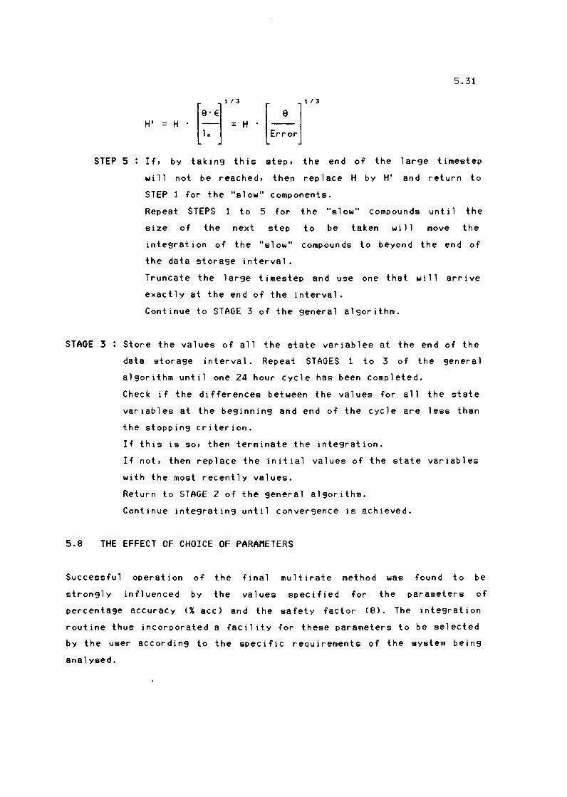
5.31

[8·EJ11J

H' = H · ~ = H

STEP 5 If, by taking this step, the end of the large timestep

wi 11 not be reached, then replace H by H' and return to

STEP 1 for the "slow" components.

STAGE 3

Repeat STEPS 1 to 5 for the "slow" compounds until the

size of the next step to be taken wi 11 move the

integration of the "slow" compounds to beyond the end of

the data storage interval.

Truncate the large timestep and use one that will arrive

exactly at the end of the interval.

Continue to STAGE 3 of the general algorithm.

Store the values of all the state variables at the end of the

data storage i nterva 1. Repeat STAGES 1 to 3 of the genera 1

algorithm until one 24 hour cycle has been completed.

Check if the differences between the values for all the state

variables at the beginning and end of the cycle are less than

the stopping criterion.

If this is so, then terminate the integration.

If not, then replace the initial values of the state variables

with the most recently values.

Return to STAGE 2 of the general algorithm.

Continue integrating until convergence is achieved.

5.8 THE EFFECT OF CHOICE OF PARAMETERS

Successful operation of the final mul t irate method was found to be

strongly influenced by the values specified for the parameters of

percentage accuracy <X ace) and the safety factor (0). The integration

routine thus incorporated a facility for these parameters to be selected

by the user according to the specific requirements of the system being

analysed.

5.32

5.8.1 The effect of percentage accuracy

Once the accuracy requirement has been specified, the integration

routine uses this value to calculate the limiting value of the local

error (E in Eq 5.13). Since E controls the selection of subsequent

stepsizes, it exerts a significant effect on the computational effort

required to perform the integration.

Figure 5.3 shows the effect of different accuracy specifications on the

behaviour of the "fast" variable Ss over a typical integration period of

an hour when the input to the system is held constant and the

integration is initiated at the solution i.e. the values of Ss should

remain constant. Three different accuracy requirements were tested!

1.0X, 0.1" and 0.01". The results are presented in Table 5.1.

When the percentage accuracy was specified as 1.0", the size of the

small timestep was, on average, 12 minutes long. Seven integration steps

were necessary to reach the end of the interval. However, this includes

two steps that were rejected when the accuracy requirements were not

met. In addition, the response of Ss was unstable, oscillating more

erratically as the timesteps became larger.

When the accuracy requirement was specified as 0.01", eleven steps were

necessary to reach the end of the ti me i nterva 1, the average step 1 ength

being 8 minutes. Only one of the steps failed to satisfy the error

tolerance and the response of the variable Ss remained stable at all

times. The price paid for the stability of the solution response is the

necessity to use small step lengths throughout the integration and thus

increase the computational effort expended. Examination of Figure 5.3

shows that, for this case, an accuracy requirement of 0.1" appears to

meet the demands of stability whilst at the same time not requiring an

excessive amount of computational effort, the average steplength being

10.6 minutes, with a very small oscillation in the response of Ss.

5.33

5.8.2 The effect of the safety factor, 8

Dahlquist and Bjorck (1974> recommend using a safety factor, 0 ~ 0.8 to

account for the fact that error estimates are only approximations. To

examine how the specification of this factor affected the integration,

three different values for 0 were selected and tested in the integration

problem outlined in Section 5.8.1. Figure 5.4 shows the effect of the

choice of 0 on the step sizes permitted. When a small magnitude for 0 of

0.5 was specified, steplengths greater than 16 minutes were never

permitted, and were generally much shorter. The average stepsize for the

integration interval was 8.3 minutes and 9 steps were required to reach

the end of the interval. Only one of these was unsuccessful. (See

Table 5.3>.

On the other hand, when a large 0 of 0.9 was specified, steplengths were

generally longer (average length 10.3 minutes> with a largest steplength

of 19.3 minutes. However, of the eleven steps required to reach the end

of the interval, four were unsuccessful. In the light of this, it would

appear that some intermediate value of 0 would offer the most favourable

balance between the number of steps required to complete the integration

and the possibility of each of these steps being successful. For the

purposes of simulation, a 0 value of 0.75 was selected as fulfilling

these requirements most appropriately.

5.9 FINAL COMMENTS ON PARTITIONING IN THE MULTIRATE METHOD

5.9.1 The effect of Xa as a "fast" or "slow" component

As noted in Section 5.7, the dynamics of Xs, the particulate substrate,

were difficult to classify as either "fast" or "slow", and there was a

general indication that this compound should occupy some "intermediate"

category. However, as the creation of an additional class of compounds

was not feasible, the effect of placing this compound in either the

"fast" or "slow" categories was examined.

5.34

3.448

3.446 0.01 %

0.1 % 3.444

3.442

3.44

3.438 -t") 3.436 I E 3.434 0\ '-'

Ill 3.432 Vl

3.43

3.428

3.426

3.424

3.422

3.42

0 20 40 60

Time (minutes)

Figure 5.3 The effect of accuracy specifications on the behaviour of

the variable Sa

X accuracy

0.01 X

0.10 X

1.00 X

Table 5.2

Number of Number of Average steps failures stepsize

11 1 8 .1 111ins

10 3 10.6 111i ns

7 2 12.0 mins

The effect of accuracy specifications on the behaviour of

the.stepping routine

5.35

20 19

18 17

"'"' 16 U)

C 15 E 14 '-"

a. 13 Cl) .....

12 U) Cl)

E 1 1 .....

10 0 9 E U) 8 .... 0 7 Cl) 6 N vi 5

4 3

2

1 3 5 7 9 1 1

Step number

Figure 5.4 The effect of the safety factor on the size of the small

timestep

Safety factor (0)

0.50

0.75

0.90

Table 5.3

Number of Number of Average steps failures stepsize

9 1 8.3 11ins

10 3 10.6 •ins

11 4 10.3 11ins

The: effect of the safety factor on the behaviour of the

eteppin9 routine

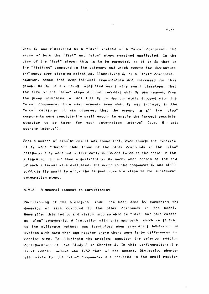
5.36

IJhen Xs was classified as a "fast" instead of a "slow" component, the

sizes of both the "fast" and "slow" steps remained unaffected. In the

case of the "fast" steps, this is to be expected, as it is Ss that is

the "l imitin9" compound in the cate9ory and which exerts the dominatin9

influence over stepsize selection. Classifyin9 Xs as a "fast" component,

however,· means that computational reQuirements are increased for this

9roup, as Xs is now bein9 inte9rated using many small timesteps. That

the size of the "slow" steps did not increase when Xs was removed from

the group indicates in fact that Xs is appropriately grouped with the

"slow"· compounds. This was because, even when Xs was included in the

"slow" category, it was observed that the errors in all the "slow"

components were consistently small enough to enable the lar9est possible

stepsize to be taken for each inte9ration interval (i.e. H = data

storage interval).

From a number of simulations it was found that, even thou9h the dynamics

of Xs were "faster" than those of the other compounds in the "slow"

category, they were not sufficiently different to cause the error in the

integration to increase si9nif'icantly. As such, when errors at the end

of each interval were evaluated, the error in the component Xs was still

sufficiently small to allow the lar9est possible stepsize for subseQuent

inte9ration steps.

5.9.2 A seneral comment on partitioninS

Partitionin9 of the biolo9ical model has been done by comparing the

dynamics of each compound to the other compounds in the model.

Generally, this led to a division into soluble as "fast" and particulate

as "slow" components. A limitation with this approach, which is general

to the multirate method, was identified when simulatin9 behaviour in

systems with more than one reactor where there were lar9e differences in

reactor size. To illustrate the problem, consider the selector reactor

confi9uration of Case Study 2 in Chapter 4. In this confi9uration, the

first reactor llolume was 1/32 that of the second, Obviously, shorter

step sizes for the "slow" compounds, are reQuired in the small reactor

5.37

with the short retention time than in the larger reactor, Similarly f'or

the "f'ast" compounds in each reactor. However, because one step length

is chosen f'or each group, the choice of' the stepsize in f'act is

controlled by the variables in the small reactor. This steplength may be

unnecessarily small f'or the compounds in the larger reactor. In f'act,

the situation could be encountered where, f'or optimal multirate

ef'f'iciency, stepsizes f'or "f'ast" compounds in large reactors should be

larger than stepsizes f'or "slow" compounds in small reactors. This

problem arises because partitioning is on the basis of' the model and not

on the basis of' individual compounds within the configuration of'

interest.

The limitation above could be overcome if' automatic or dynamic

partitioning were implemented. However, this possibilty has already been

excluded and the limitation had to be accepted. On the other hand, it

was f'elt that generating the division on the basis of' the biological

model generalised the method and simplified its implementation

considerably.

5 .10 CLOSURE

A mu 1 ti rate integration procedure has been f'oun d to be appropriate f'or

biological systems. In these systems, the dynamics of' the dif'f'erent

compounds clearly divide into two groups, a "f'ast" group requiring short

integration steps and a "slow" group f'or which the steps can be larger.

Within each group, the range of' dynamics is small compared to the

dif'f'erence between the two groups. A general guideline f'or partitioning

a biological system is that it appears that soluble compounds can be

grouped as "f'ast" and particulate compounds as "slow".

Some specific considerations should be noted as regards implementation

of' the multirate technique:

(i) Partitioning of' the

analysis ~an lead to

multirate technique.

system on the

inef'f'iciencies in

This is one of'

basis of' the model under

the implementation of' the

the f'ew drawbacks of' the

5.38

method. In practice, partitionins on the basis of practical

experience and by trial examination of the system was found to be

the most flexible approach.

(ii) A predictor-corrector method with only one application of the

corrector as proposed by Lapidus (1971) was found to be

particularly suited to the dynamics of the system.

(iii) The steplensth adjustment procedure proposed by Dahlquist and

Bjorck (1974) has been found to be appropriate. The success of

this procedure rests on the fact that it al ways uses the l arsest

possible stepsize without allowins the errors to accumulate in the

system. The method was found to be superior to Gear's method of

steplensth halvins or doublins.

(iv) Discretion should be excercised in the choice of parameters such

as percentase accuracy and the safety factor, 9.

The objective of

techniques which

this

can be

CHAPTER SIX

CONCLUSIONS

investi9ation was to develop

applied to the modellin9 and

biolo9ical reaction system behaviour.

and evaluate

simulation of

The model used as the basis for the investi9ation was a reduced version

of the bi o 109 i ca 1 mode 1 proposed by the IAIJPRC Task Group for

mathematical modelling in wastewater treatment design. This limited

model had the advanta9e of being easily manageable in terms of analysis

and presentation of the simulation techniques. At the same time the

model incorporated a ran9e of kinetic formulations encountered with

biolo9ical 9rowth applications. Once the model had been selected, mass

balance equations for each compound in each reactor could be formulated.

These constitute a set of simultaneous non-linear ordinary differential

and al9ebraic equations which, when solved, characterised the system

behaviour. Two situations were considered for the purposes of

simulation:

Ci) steady state conditions, where the system operates under conditions

of constant influent flow and load:

(ii) dynamic conditions, where the influent to the system varies with

time, usually in a cyclic pattern.

The steady state problem:

Under steady state conditions the derivative terms in the differential

equations fall away and the problem

of non-linear al9ebraic equations.

solution were evaluated:

(i) Direct linearisation

(ii) Successive substitution

(iii) The secant method of We9stein

is reduced to one of solvin9 a set

Five approaches to computin9 the

(iv) Newton's method

Cv) Broyden's method

6.2

These methods were evaluated through application to five test cases

representing the types of system configuration encountered in practice.

The most efficient technique for the case studies was found to be

Newton'• •ethod with a finite difference approximation to the Jacobian.

The dynamic problem:

The dynamic problem involves solving a set of coupled ordinary

differential equations. The use of a multirate technique in combination

with variable stepsizes for the integration was found to be a most

successful approach. Aspects of particular importance concerning the

method are:

Ci) The system variables are partitioned into two groups: those with

"fast" and those with "slow" dynamics. These two groups are

integrated separately with different step lengths to reduce

computational effort.

(ii) A general guideline for partitioning a biological system is that

it appears that soluble compounds can be grouped as "fast" and

particulate compounds as "slow".

(iii) The multirate method was based on the approach of Gear (1984). For

step length adjustment, however, the approach of Dahlquist and

Bjorck (1974) was found to be more efficient than the

halving/doubling approach suggested by Gear. IJith Dahlquist and

Bjorck's approach the magnitude of the adjustments to the

steplength are based on the magnitude of the integration error.

R .1

LIST OF REFERENCES

Aitken A C (1925). On Bernoulli's Numerical Solution of Algebraic

tquations. Proc. Roy. Soc. Edinbur9h, 46, 289.

Borland International Inc (1985). Turbo Pascal Version 3.0. Borland

International Inc. Scotts Valley. CA.

Broyden C G (1965). "A class of methods for solving non-linear

simultaneous equations". Math Co11p, 19, 577-593.

Broyden CG (1969). "A new double rank minimisation algorithm". AMS

notices, 16, 670.

Dahlquist G and A Bjorck (1974). Numerical Methods. Prentice Hall Inc.

Englewood Cliffs. New Jersey.

Dennis J R (Jnr) and J J More (1977). Quasi-Newton Methods, motivation

and theory. SIAM Rev, 19, 46 - 49.

Dennis J R (Jnr) and R B Schnabel (1983).

Unconstrained Optimisation and Non Linear

Hall Inc. Englewood Cliffs. New Jersey.

Numerical Methods for

Equations. Prentice

Dold P L and G v R Marais (1985). Evaluation of the general activated

sludge model incorporating specifications proposed by the IAWPRC

task Group. Presented at the IAWPRC specialised seminar on

Modelling of Biological Wastewater Treatment, Copenhagen,

Denmark. Wat.Sci.Tech., 18, 63-89.

Gear C W (1971>. Numerical Initial Value problems in ordinary

differential equations. Prentice Hall Inc. Englewood Cliffs. New

Jersey.

R.2

Gear CW (1984). Multirate linear multistep methods. Bit, 24, 484-502.

Grau P, P M Sutton, M Henze, S Elmaleh, C P L Grady, W Gujer and J

Koller (1982). Recommended notation for use in the description of

biolo9ical wastewater treatment processes. Water Research, 16,

1501.

Henze M, CP Leslie Grady, W Gujer, G V R Marais and T Matsuo (1987).

Abbreviated Report: A 9eneral model for sin9le-slud9e wastewater

treatment systems. Water Research, 21, 5, 505-515.

Johnston R L (1982>. Numerical Methods, A Software Approach. John Wiley

and Sons. Canada.

Lambert J D (1979). Computational Methods • John Wiley and Sons. Great

Britain.

Lapidus L and J H Seinfeld (1971). Numerical Solution of Ordinary

Differential Equations. Academic Press. New York.

Levenspiel O (1972). Chemical Reaction En9ineerin9. 2nd Ed. John Wiley

and Sons. New York.

Myers A L and W H Sieder (1976). Introduction to Chemical En9ineerin9

and Computer Calculations. Prentice-Hall, Inc. En9lewood Cliffs.

New Jersey.

Orailo9lu A (1983). Software desi9n issues

hierachical display editors. Rept No.

Computer Sci. Univ. Illinois.

in the implementation of

UIUCDCS-R-83-1139. Dept.

Petersen E E. <1965). Chemical reaction analysis. Prentice Hall.

En9lewood Cliffs. New Jersey.

R.3

Reklaitis G V (1983). Introduction to Material and Energy Balances. John

Wiley and Sons. New York.

Sargent R W H (1981). A Review of Methods for solving non-linear

Algebraic Equaitons. In RSH Mah and W D Sieder (eds). Foundations

of Computer-Aided Chemical Process Design. Engineering

Foundation, New York, Vol 1, 22-76,

Steffensen J F (1933). Remarks on Iteration. Skand. Aktuar. Tidskr, 16,

64 - 72.

Water Research Commission (1984). Theory, design and operation

nutrient removal activated sludge processes. Published by

Water Research Commission. PO Box 824. Pretoria. 0001.

of

the

Wegste in J H ( 1958>. Accelerating Convergence of Iterative Processes.

C Offill • ACM, 1 , < 6 > , 9 •

Westerberg A W, H P Hutchison, R L Motard and P Winter (1979). Process

Flowsheeting. Cambridge University Press.

modelling techniques for biological systems - core.ac.uk in an attempt to improve the convergence...

Documents