modelling techniques and novel configurations for meander
TRANSCRIPT

Modelling Techniques and Novel Configurations
for Meander-line-coil Electromagnetic Acoustic
Transducers (EMATs)
A thesis submitted to the University of Manchester for the degree of
Doctor of Philosophy
in the Faculty of Engineering and Physical Sciences
2016
By
Yuedong Xie
School of Electrical and Electronic Engineering
List of Contents
2
LIST OF CONTENTS
LIST OF CONTENTS ...................................................................................................... 2
LIST OF FIGURES .......................................................................................................... 6
LIST OF TABLES .......................................................................................................... 15
NOMENCLATURE ........................................................................................................ 16
ABSTRACT ..................................................................................................................... 18
DECLARATION ............................................................................................................. 19
COPYRIGHT STATEMENT ........................................................................................ 20
ACKNOWLEDGEMENTS ............................................................................................ 21
Chapter 1 Introduction ............................................................................................... 22
1.1 Motivation .......................................................................................................... 22
1.2 Aim and Objectives ............................................................................................ 23
1.3 Contributions ...................................................................................................... 23
1.4 Organization of thesis ......................................................................................... 24
1.5 List of Publications ............................................................................................. 25
Chapter 2 EMAT background ................................................................................... 27
2.1 Introduction ........................................................................................................ 27
2.2 Coupling Mechanisms of EMATs ...................................................................... 27
2.2.1 Lorentz Force Mechanism........................................................................... 27
2.2.2 Magnetostriction Mechanism ...................................................................... 28
2.2.3 Advantages and Disadvantages of EMATs................................................. 29
2.3 Types of EMATs ................................................................................................ 31
2.3.1 Major Types of Mechanical Waves ............................................................ 31
2.3.2 Classification of EMATs............................................................................. 34
2.4 State-of-the-art in EMAT Modelling ................................................................. 38

List of Contents
3
2.5 Conclusions ........................................................................................................ 40
Chapter 3 FDTD for Ultrasonic Modelling ............................................................... 41
3.1 Ultrasonic Testing Techniques ........................................................................... 41
3.1.1 Phased Array Techniques ............................................................................ 41
3.1.2 Ultrasonic Testing Methods ........................................................................ 44
3.2 FDTD Method for Ultrasonic Modelling ........................................................... 47
3.2.1 Elastodynamic Equations ............................................................................ 47
3.2.2 The Finite-difference time-domain (FDTD) Method .................................. 48
3.3 Ultrasonic Phased Array Modelling with FDTD ............................................... 49
3.4 Novel Radiation Pattern with Hilbert Transformation ....................................... 53
3.4.1 Hilbert Transformation................................................................................ 53
3.4.2 Novel Radiation Pattern with the Hilbert Transformation .......................... 54
3.5 Near Field and Far Field Modelling ................................................................... 55
3.5.1 Near Field Analysis ..................................................................................... 56
3.5.2 Far Field Analysis ....................................................................................... 61
3.5.3 Conclusions of Section 3.5 .......................................................................... 63
3.6 Scattering Modelling .......................................................................................... 64
3.7 Conclusions ........................................................................................................ 66
Chapter 4 Development and Validation of A Novel Method for Modelling
Meander-line-coil EMATs Operated on Lorentz Force Mechanism ......................... 68
4.1 Introduction ........................................................................................................ 68
4.1.1 Modelling Geometry ................................................................................... 68
4.2 EMAT-EM Modelling ........................................................................................ 69
4.2.1 Classic Dodd and Deeds Solutions ............................................................. 69
4.2.2 Adapted Analytical Solutions for A Straight Wire ..................................... 73
4.2.3 Validation and Comparison with FEM ....................................................... 74

List of Contents
4
4.2.4 Analytical EMAT-EM Modelling ............................................................... 80
4.3 Novel Methods for EMATs ................................................................................ 85
4.3.1 The Combination of EM and US Models ................................................... 85
4.3.2 The Propagation of Rayleigh Waves........................................................... 87
4.3.3 Displacement Calculation and Depth Profile .............................................. 88
4.3.4 The Effect of the Fractional Bandwidth ...................................................... 90
4.4 The Property of Rayleigh Waves ....................................................................... 92
4.4.1 Radiation Pattern ......................................................................................... 92
4.4.2 Beam Features ............................................................................................. 93
4.5 EMAT-receiving Mechanism ............................................................................. 95
4.6 Experimental Validations ................................................................................... 96
4.6.1 Experiments Set-up ..................................................................................... 96
4.6.2 Received Signals from Experiments ........................................................... 98
4.6.3 Validation of EMAT Models with Experiments ......................................... 99
4.7 EMAT Scattering Phenomena .......................................................................... 102
4.7.1 Modelling of Rayleigh Waves’ Scattering ................................................ 102
4.7.2 Experiments and Validations .................................................................... 106
4.8 Modelling of Unidirectional Rayleigh Waves EMATs .................................... 108
4.9 Conclusions ...................................................................................................... 113
Chapter 5 Directivity Analysis of Conventional Meander-line-coil EMATs ....... 115
5.1 Introduction ...................................................................................................... 115
5.2 The Analytical Solution to the Radiation Pattern of Rayleigh Waves on the
Surface of the Material ................................................................................................ 115
5.3 Beam Directivity Analysis of the Conventional Constant-length Meander-line-
coil (CLMLC) ............................................................................................................. 117
5.3.1 Wholly Analytical Models ........................................................................ 118

List of Contents
5
5.3.2 The Effect of the Length of the Conventional Constant-length Meander-line-
coil (CLMLC) on Radiation Pattern ....................................................................... 121
5.4 Experimental Results ........................................................................................ 123
5.5 Conclusions ...................................................................................................... 125
Chapter 6 Novel Configurations for Meander-line-coil EMATs .......................... 127
6.1 Introduction ...................................................................................................... 127
6.2 Novel Variable-length Meander-line-coil (VLMLC) EMATs ......................... 128
6.2.1 Wholly Analytical Models for the Novel Variable-length Meander-line-coil
(VLMLC) EMATs .................................................................................................. 129
6.2.2 Analysis of Beam Properties of Rayleigh Waves Generated by the Novel
Variable-length Meander-line-coil (VLMLC) EMATs .......................................... 130
6.3 Novel Multi-directional Meander-line-coil EMATs ........................................ 138
6.3.1 Introduction ............................................................................................... 138
6.3.2 Four-directional Meander-line-coil (FDMLC) EMATs............................ 138
6.3.3 Six-directional Meander-line-coil (SDMLC) EMATs .............................. 143
6.3.4 Discussion ................................................................................................. 146
6.4 Conclusions ...................................................................................................... 146
Chapter 7 Conclusions and Recommendations for Future Work ........................ 148
7.1 Conclusions ...................................................................................................... 148
7.1.1 FDTD Method for Simulating US Behaviours ......................................... 148
7.1.2 Vertical Plane Modelling for EMATs ....................................................... 149
7.1.3 Surface Plane Modelling for EMATs ....................................................... 150
7.1.4 Novel Configurations for EMATs ............................................................ 151
7.2 Recommendations for Future Work ................................................................. 152
REFERENCES .............................................................................................................. 154

List of Figures
6
LIST OF FIGURES
Figure 2-1: Schematic of the Lorentz force mechanism. From [19]. ................................... 27
Figure 2-2: Microscopic process of the field induced magnetostriction. H is the external
magnetic field; ∆l is the deformation due to the reorientation of the magnetic domain,
which is simplified represented by an elliptic shape. From [18]. ........................................ 29
Figure 2-3: EMATs operated on the magnetostriction mechanism. εd is the dynamic stress,
εs is the static stress, and εr is the resultant stress. ................................................................ 29
Figure 2-4: Longitudinal waves. The black arrow denotes the direction of the wave
propagation; red arrows denote directions of the particle motion. From [50]. .................... 31
Figure 2-5: Shear waves. The black arrow denotes the direction of the wave propagation;
red arrows denote directions of the particle motion. From [50]. ......................................... 32
Figure 2-6: Rayleigh waves. The black ellipse denotes the particle motions. From [54]. ... 32
Figure 2-7: Modes of Lamb waves. (a), symmetric mode; (b), anti-symmetric mode. The
black arrows denote the displacement of the particle; black curves denote the resulting
Lamb waves. From [58]. ...................................................................................................... 33
Figure 2-8: The cross-sectional view of a normal longitudinal wave EMAT. The white
hollow arrows denote the direction of the static magnetic field; the grey arrows denote the
direction of the Lorentz force; the solid black arrow means the direction of wave
propagation. From [19, 20]. ................................................................................................. 34
Figure 2-9: The cross-sectional view of normal shear waves EMATs. The white hollow
arrows denote the direction of the static magnetic field; the grey arrows denote the
direction of the Lorentz force; the solid black arrows mean the direction of wave
propagation. Adapted from [19, 20]. .................................................................................... 35
Figure 2-10: The structure of the periodic-permanent-magnet (PPM) EMAT to generate
SH waves. From [16]. .......................................................................................................... 35
Figure 2-11: The cross-sectional view of the PPM EMAT. From [48]. .............................. 36

List of Figures
7
Figure 2-12: The structure of the meander-line-coil EMAT to generate SH waves. From
[16]. ...................................................................................................................................... 37
Figure 2-13: The structure of a meander-line-coil EMAT to generate Rayleigh waves.
From [16, 34]. ...................................................................................................................... 37
Figure 3-1: Phased array techniques: steering and focusing [10]. ....................................... 42
Figure 3-2: A model used for time delays calculation for steering. ..................................... 43
Figure 3-3: A model for time delays calculation for focusing. ............................................ 44
Figure 3-4: Ultrasonic pulse-echo method. (a), Inspection diagram; (b) Received signals. 45
Figure 3-5: Ultrasonic through-transmission method. (a), Inspection diagram; (b) Received
signals. .................................................................................................................................. 45
Figure 3-6: Ultrasonic pitch-catch method. ......................................................................... 46
Figure 3-7: Modelling geometry for steering (a) and focusing (b). ..................................... 49
Figure 3-8: Pure sine wave; (a) the time domain signal of the pure sine wave; (b) the
magnitude of the pure sine wave’s Fourier transform [75]. ................................................. 51
Figure 3-9: Gaussian-modulated sine wave; (a) the time domain signal of the Gaussian-
modulated sine wave; (b) the magnitude of the Gaussian-modulated sine wave’s Fourier
transform [75]....................................................................................................................... 51
Figure 3-10: Steering techniques: firing elements at prescribed calculated times, the
wavefront is steered at 00, 300, 600, 900 respectively. .......................................................... 52
Figure 3-11: Focusing techniques: the wavefront is focused at the prescribed focal point. 53
Figure 3-12: Signals to indicate the arrival times of ultrasound waves. .............................. 54
Figure 3-13: (a), Radiation pattern for the beam steered at 300; (b), radiation pattern for
studying beam features. ........................................................................................................ 55
Figure 3-14: The description of the focal length and the steering angle. ............................. 57
Figure 3-15: The radiation pattern of the focusing behaviour in the near field. .................. 57

List of Figures
8
Figure 3-16: Beam features of focusing within the near filed. (a), Beam directivity of the
focusing behaviour; (b) Field distribution along the steering angle of the focusing
behaviour. ............................................................................................................................. 58
Figure 3-17: Radiation pattern of the steering behaviour with a steering angle of 300. ...... 59
Figure 3-18: Beam features of steering within the near filed. (a), Beam directivity of the
steering behaviour; (b) Field distribution along the steering angle of the steering behaviour.
.............................................................................................................................................. 59
Figure 3-19: The beam directivity of the focusing behaviour at different radial lengths. ... 61
Figure 3-20: Radiation pattern of the focusing behaviour in the far field. .......................... 61
Figure 3-21: Beam features of focusing in the far field: (a) beam directivity at a focal
length of 150 mm, (b) field distribution along the steering angle 300. ................................ 62
Figure 3-22: Beam features of steering in the far field: (a) beam directivity at a radial
length of 150 mm, (b) field distribution along the steering angle 300. ................................ 63
Figure 3-23: The geometry of scattering modelling. ........................................................... 65
Figure 3-24: Wave propagation of the scattering modelling at different times. .................. 66
Figure 3-25: The received signals from the receiving array. (a), directly transmitted signals;
(b), the scattered longitudinal waves; (c), the scattered shear waves................................... 66
Figure 4-1: The configuration of a typical meander-line-coil EMAT. ................................ 69
Figure 4-2: A model built by Dodd and Deeds [79]. ........................................................... 70
Figure 4-3: Geometry for the conductor with only one layer. ............................................ 71
Figure 4-4: For a circular coil, the distribution of the magnitude of the vector potential
within the conductor. ............................................................................................................ 72
Figure 4-5: For a circular coil, the vector potential distribution along the surface of the
conductor (𝒙=0). .................................................................................................................. 73

List of Figures
9
Figure 4-6: For a large-radius circular coil, the vector potential distribution within the
conductor. ............................................................................................................................. 74
Figure 4-7: For a large-radius circular coil, the vector potential along the surface of the
conductor (𝒙=0). .................................................................................................................. 74
Figure 4-8: (a), the model built with Maxwell Ansoft; (b), mesh of the model. ................. 75
Figure 4-9: In FEM solver, the energy error versus the number of triangles. ...................... 75
Figure 4-10: At 10 kHz, the vector potential distribution within the stainless steel plate. (a),
the analytical method; (b) the finite element method (FEM). .............................................. 76
Figure 4-11: At 10 kHz, the vector potential along the surface of the stainless steel plate.
(a), (b) and (c) denotes the magnitude, the real part, and the imaginary part of the vector
potential respectively. .......................................................................................................... 77
Figure 4-12: At 1 MHz, the vector potential distribution within the stainless steel plate. (a),
the analytical method; (b) the finite element method (FEM). .............................................. 78
Figure 4-13: At 1 MHz, the vector potential along the surface of the stainless steel plate.
(a), (b) and (c) denotes the magnitude, the real part, and the imaginary part of the vector
potential respectively. .......................................................................................................... 78
Figure 4-14: With various lift-offs, the distribution of the real part of the vector potential
along the surface of the stainless steel plate......................................................................... 79
Figure 4-15: 2D model of the EMAT-EM simulation. ........................................................ 81
Figure 4-16: The real part of the vector potential produced by a meander-line-coil. .......... 81
Figure 4-17: The real part of the induced eddy current produced by a meander-line-coil. . 82
Figure 4-18: The eddy current distribution along the surface of the stainless steel plate
(x=0). .................................................................................................................................... 82
Figure 4-19: The mesh of the static magnetic field modelling. ........................................... 83
Figure 4-20: The relationship between the elements number and the energy error for the
static magnetic field modelling. ........................................................................................... 83

List of Figures
10
Figure 4-21: The vector of the magnetic flux density generated by the permanent magnet.
.............................................................................................................................................. 83
Figure 4-22: The distribution of the magnitude of the magnetic flux density within the
stainless steel plate. .............................................................................................................. 84
Figure 4-23: L The distribution of the magnetic flux density along the surface of the
stainless steel plate (x=0). .................................................................................................... 84
Figure 4-24: The distribution of the Lorentz force density along the surface of the stainless
steel plate. ............................................................................................................................. 85
Figure 4-25: The combination between the EM model and the US model. ......................... 86
Figure 4-26: The excitation signal for wire 1 and wire 2. .................................................... 87
Figure 4-27: The wave propagation at 18 µs and 35 µs after firing respectively. ............... 88
Figure 4-28: The received signals; (a), signals received by the receiver R1; (b), signals
received by the receiver R2. ................................................................................................. 89
Figure 4-29: The depth profile of Rayleigh waves’ displacement. ...................................... 90
Figure 4-30: The excitation signal with various fractional bandwidths. .............................. 91
Figure 4-31: The received signals with excitation signals at various fractional bandwidths.
.............................................................................................................................................. 92
Figure 4-32: (a), the radiation pattern of the EMAT-Rayleigh waves; (b), the radiation
pattern used for the analysis of beam features. .................................................................... 93
Figure 4-33: Beam directivity of Rayleigh waves. .............................................................. 94
Figure 4-34: Field distribution along the steering angle 00 of Rayleigh waves. .................. 94
Figure 4-35: The model used for calculating the induced voltage in the receiving coil. ..... 95
Figure 4-36: The schematic diagram of the experimental system. ...................................... 97
Figure 4-37: Set-up of the experimental system. ................................................................. 98

List of Figures
11
Figure 4-38: The frequency domain of the experimentally received signals. ...................... 98
Figure 4-39: The received signal from experiments. ........................................................... 99
Figure 4-40: The comparison between the simulation and the experiment. ...................... 100
Figure 4-41: The maximum amplitude of the induced voltage with various distances
between the transmitter and the receiver. ........................................................................... 101
Figure 4-42: The received signals with a meander-line-coil as the transmitter. ................ 102
Figure 4-43: The geometry of Rayleigh waves’ scattering simulation. ............................. 103
Figure 4-44: Scattering behaviours of Rayleigh waves. .................................................... 104
Figure 4-45: Received signals from R1. ............................................................................ 105
Figure 4-46: Received signals from R2. ............................................................................ 105
Figure 4-47: The comparison of the received signals from the receivers R1 and R2. ....... 106
Figure 4-48: The experimentally received signal from the receiver R1. ........................... 107
Figure 4-49: The amplitude comparison between the simulation and the experiment. ..... 108
Figure 4-50: The envelop comparison between the simulation and the experiment.......... 108
Figure 4-51: The configuration of the URW EMAT. From [23]. ...................................... 109
Figure 4-52: The wave superposition between the source 1 and the source 2. From [80]. 110
Figure 4-53: The excitation signal for the coil A and the coil B........................................ 110
Figure 4-54: The wave propagation of Rayleigh waves generated by the URW-EMAT. . 111
Figure 4-55: The received signal from the URW-EMAT. ................................................. 112
Figure 4-56: The received signal from the BRW-EMAT. ................................................. 112
Figure 4-57: The comparison between the URW and the BRW. ....................................... 113
Figure 5-1: Surface waves generated by the point source.................................................. 117

List of Figures
12
Figure 5-2: The transformation between the analytical EM model and the analytical US
model. ................................................................................................................................. 118
Figure 5-3: The Rayleigh waves’ radiation pattern on the surface of the aluminium plate.
............................................................................................................................................ 120
Figure 5-4: The model used to study the beam directivity. ............................................... 120
Figure 5-5: The beam directivity of Rayleigh waves generated by a 30mm-length meander-
line-coil EMAT. (a), the curve of the beam directivity; (b) the curve used for describing
HPBW and SLL. ................................................................................................................ 121
Figure 5-6: The beam directivity of the meander-line-coil with various lengths. ............. 122
Figure 5-7: (a), experimental set-up; (b), the scan path of the receiver; Tx means the
transmitter and Rx means the receiver. .............................................................................. 123
Figure 5-8: The measured beam directivity from experiments. ......................................... 124
Figure 5-9: Comparison between the simulated and measured results for the meander-line-
coil with a length of 10 mm (a), 20 mm (b), 30 mm (c) and 40 mm (d) respectively. ...... 125
Figure 6-1: The configuration of the variable-length meander-line-coil (VLMLC). (a), the
schematic diagram; (b), the fabricated variable-length meander-line-coil. ....................... 128
Figure 6-2: The transformation between the analytical EM model and the analytical US
model. ................................................................................................................................. 130
Figure 6-3: The radiation pattern of the variable-length meander-line-coil (VLMLC). .... 131
Figure 6-4: The beam directivity of the 50 mm variable-length meander-line-coil (VLMLC)
with a step of 8 mm. ........................................................................................................... 132
Figure 6-5: The beam directivity comparison between the conventional constant-length
meander-line-coil (CLMLC) and the novel variable-length meander-line-coil (VLMLC).
............................................................................................................................................ 132
Figure 6-6: The beam directivity of a 50 mm variable-length meander-line-coil (VLMLC).
............................................................................................................................................ 133

List of Figures
13
Figure 6-7: The comparison between the 40 mm VLMLC and the 50 mm VLMLC at
different steps. .................................................................................................................... 135
Figure 6-8: The measured beam directivity of the 50 mm VLMLC with a step of 8 mm. 136
Figure 6-9: Measured beam directivity from experiments. ................................................ 136
Figure 6-10: For 50 mm VLMLC with various steps, the comparison between the
simulated beam directivity and the measured beam directivity. ........................................ 137
Figure 6-11: Four-directional meander-line-coil (FDMLC). (a), the schematic diagram of
FDMLC; (b) the fabricated FDMLC.................................................................................. 139
Figure 6-12: The approximated configuration of the four-directional meander-line-coil
(FDMLC). .......................................................................................................................... 140
Figure 6-13: The simulated beam directivity of the four-directional meander-line-coil
(FDMLC) EMAT. .............................................................................................................. 141
Figure 6-14: The magnitude of the received Rayleigh waves............................................ 141
Figure 6-15: (a), The scan path of the receiver; (b), the experimental beam directivity. .. 142
Figure 6-16: The simulated beam directivity and the measured beam directivity of FDMLC.
............................................................................................................................................ 142
Figure 6-17: Six-directional meander-line-coil (SDMLC). (a), the schematic diagram of
SDMLC; (b) the fabricated SDMLC.................................................................................. 143
Figure 6-18: The approximated model for the six-directional meander-line-coil (SDMLC).
............................................................................................................................................ 144
Figure 6-19: The simulated beam directivity of the six-directional meander-line-coil
(SDMLC) EMAT ............................................................................................................... 144
Figure 6-20: The magnitude of the received Rayleigh waves............................................ 145
Figure 6-21: (a), The scan path of the receiver; (b), the experimental beam directivity. .. 145

List of Figures
14
Figure 6-22: The simulated beam directivity and the measured beam directivity of SDMLC.
............................................................................................................................................ 146

List of Tables
15
LIST OF TABLES
Table 2-1: The state-of-the-art in EMAT modelling............................................................ 39
Table 3-1: Parameters used for modelling steering and focusing ........................................ 50
Table 3-2: Detailed parameters used for near and far fields modelling. .............................. 56
Table 4-1: Detailed parameters used for studying analytical solutions proposed by Dodd
and Deeds. ............................................................................................................................ 72
Table 5-1: Detailed parameters used for the analytical US model..................................... 119
Table 5-2: HPBW and SSL for the meander-line-coil with various lengths...................... 123
Table 6-1: Detailed parameters used for fabricating the variable-length meander-line-coil
(VLMLC). .......................................................................................................................... 129
Table 6-2: Detailed parameters used for the EMAT-US modelling. ................................. 130
Table 6-3: Comparison: Beamwidth and the Sidelobe Level. ........................................... 133
Table 6-4: HPBW and SLL at various steps. ..................................................................... 134
Table 6-5: Detailed parameters used for the four-directional meander-line-coil (FDMLC).
............................................................................................................................................ 139
Nomenclature
16
NOMENCLATURE
Abbreviations and Acronyms
EMATs Electromagnetic Acoustic Transducers
EM Electromagnetic
US Ultrasound
FEM Finite Element Method
FDTD Finite-Difference Time-Domain
VLMLC Variable-Length Meander-Line-Coil
FDMLC Four-Directional Meander-Line-Coil
SDMLC Six-Directional Meander-Line-Coil
DC Direct Current
AC Alternating Current
SH Shear Horizontal
SV Shear Vertical
PPM Periodic-Permanent-Magnet
CFL Courant–Friedrichs–Lewy
PML Perfectly Matched Layer
FFT Fast Fourier Transform
RMSE Root-Mean-Square Error
L waves Longitudinal Waves
S waves Shear Waves
RRW Reflected Rayleigh Waves
SRW Scattered Rayleigh Waves
DRW Directly transmitted Rayleigh Waves
BRW Bidirectional Rayleigh Waves

Nomenclature
17
URW Unidirectional Rayleigh Waves
IEEE Institute of Electrical and Electronics Engineers
RL Receiver on the Left
RR Receiver on the Right
HPBW Half Power Beamwidth
SLL Sidelobe Level
CLMLC Constant-Length Meander-Line-Coil

Abstract
18
ABSTRACT
Name of University: The University of Manchester
Candidate’s Name: Yuedong Xie
Degree Title: Doctor of Philosophy
Thesis Title: Modelling Techniques and Novel Configurations for Meander-line-coil
Electromagnetic Acoustic Transducers (EMATs)
Date: July 2016
Electromagnetic acoustic transducers (EMATs) are increasingly used in industries due to
their attractive features of being non-contact, cost-effective and the fact that a variety of
wave modes can be generated, etc. There are two major EMATs coupling mechanisms: the
Lorentz force mechanism for conductive materials and the magnetostriction mechanism for
ferromagnetic materials; EMATs operated on Lorentz force mechanism are the focus of
this study.
This work aims to investigate novel efficient modelling techniques for EMATs, in order to
gain further knowledge and understanding of EMATs wave pattern, how design parameters
affect its wave pattern and based on above propose and optimise novel sensor structures.
In this study, two novel modelling methods were proposed: one is the method combining
the analytical method for EM simulation and the finite-difference time-domain (FDTD)
method for US simulation for studying the Rayleigh waves’ properties on the vertical plane
of the material; the other one is the method utilizing a wholly analytical model to explore
the directivity of surface waves. Both simulations models have been validated
experimentally. The wholly analytical model generates the radiation pattern of surface
waves, which lays a solid foundation for the optimum design of such sensors. The beam
directivity of surface waves was investigated experimentally, and results showed the length
of wires has a significant effect on the beam directivity of Rayleigh waves.
A novel configuration of EMATs, variable-length meander-line-coil (VLMLC), was
proposed and designed. The beam directivity of surface waves generated by such novel
EMATs were analytically investigated. Experiments were conducted to validate such novel
EMATs models, and results indicated that such EMATs are capable of supressing side
lobes, and therefore resulting in a more concentrated surface waves in the desired direction.
Further, another two novel configuration of EMATs, the four-directional meander-line-coil
(FDMLC) and the six-directional meander-line-coil (SDMLC), were proposed and
designed; results showed these EMATs are capable of generating Rayleigh waves in
multiple directions and at the same time suppressing side lobes.

Declaration
19
DECLARATION
No portion of the work referred to in this thesis has been submitted in support of an
application for another degree of qualification of this or any other university or other
institution of learning.

Copyright Statement
20
COPYRIGHT STATEMENT
i. The author of this thesis (including any appendices and/or schedules to this thesis)
owns certain copyright or related rights in it (the “Copyright”) and he has given The
University of Manchester certain rights to use such Copyright, including for
administrative purposes.
ii. Copies of this thesis, either in full or in extracts and whether in hard or electronic copy,
may be made only in accordance with the Copyright, Designs and Patents Act 1988
(as amended) and regulations issued under it or, where appropriate, in accordance with
licensing agreements which the University has from time to time. This page must form
part of any such copies made.
iii. The ownership of certain Copyright, patents, designs, trade marks and other
intellectual property (the “Intellectual Property”) and any reproductions of copyright
works in the thesis, for example graphs and tables (“Reproductions”), which may be
described in this thesis, may not be owned by the author and may be owned by third
parties. Such Intellectual Property and Reproductions cannot and must not be made
available for use without the prior written permission of the owner(s) of the relevant
Intellectual Property and/or Reproductions.
iv. Further information on the conditions under which disclosure, publication and
commercialisation of this thesis, the Copyright and any Intellectual Property and/or
Reproductions described in it may take place is available in the University IP Policy
(see http://documents.manchester.ac.uk/DocuInfo.aspx?DocID=487), in any relevant
Thesis restriction declarations deposited in the University Library, The University
Library’s regulations (see http://www.manchester.ac.uk/library/aboutus/regulations)
and in The University’s policy on Presentation of Theses.

Acknowledgements
21
ACKNOWLEDGEMENTS
I would like to express my sincere gratitude to my supervisor Dr. Wuliang Yin and co-
supervisor Prof. Anthony Peyton, for their continuous support of my Ph.D study and
research, for their patience, motivation and encouragement. Their guidance helped me in
all the time of research and writing of this thesis.
Besides my supervisors, I would like to thank Prof. Zenghua Liu in Beijing University of
Technology, for providing the experimental instrument, which is really helpful for me to
carry out the experimental study. Also, I would like to thank Mr Peng Deng, Mr Yanan Hu
and Miss Muwen Xie, for setting up the experiments in Beijing University of Technology.
My thanks go to Professor Emmanuel Bossy in Langevin Institute, for his contributions to
the open source FDTD solver, SimSonic, from which some of the simulations contained in
this work were carried out.
I would like to express my appreciation to my colleagues in SISP group in University of
Manchester, for the research discussions and communications, and for all the fun we have
had in the last four years.
Last but not the least, I would like to thank my family: my parents Jianzhi Xie and
Zhuanmei Zhao, my sister Miaoling Xie, my brother-in-law Xiaobo Huo, my niece
Mengxuan Huo, and my girlfriend Dr. Weiwei An, for supporting me spiritually
throughout my life.

CHAPTER 1 Introduction
22
Chapter 1 Introduction
In this chapter, the motivation, aim, objectives and contributions of this study are
introduced, followed by the organisation of the thesis.
1.1 Motivation
Ultrasonic non-destructive testing, which normally operates at a frequency with a range
from 20 kHz to 100 MHz, is a branch of non-destructive testing techniques. This technique
is based on the ultrasound waves’ propagation within the test piece: ultrasound waves are
generated into the test piece; when ultrasound waves encounter any discontinues or
boundaries of the test piece, they are scattered and picked up by the transducer. Hence
ultrasonic non-destructive testing is able to perform thickness measurement, crack
detection and material characterisation [1-6].
The transducer frequently used for the ultrasonic non-destructive testing is piezoelectric
ceramics or crystals [5-7]. The piezoelectric transducer offers several advantages, such as
good penetration depth, mechanical flexibility, insensitive to electromagnetic fields and
radiation, ease of use and relatively low cost, etc. [8-10]. However, one primary
disadvantage of the piezoelectric ultrasonic testing is the need to have good sonic contact
between the piezoelectric transducer and the test piece, typically by means of a couplant
for acoustic impedance matching [9, 10]. This drawback places limits on piezoelectric
transducers in several applications, such as high temperature detecting, low temperature
detecting, and moving samples detecting, etc. [9, 11].
There are mainly two non-contact ultrasonic techniques, laser-based ultrasonic techniques
and Electromagnetic Acoustic Transducers (EMATs) techniques; while the former is
relatively more expensive [12]. EMATs techniques are the focus of this study due to their
attractive features of being non-contact, cost-effective and the fact that a variety of wave
modes can be generated, etc. Although considerable works have been reported on the
study of EMATs, there are still many important issues which need further investigation,
especially advanced and efficient modelling methods are needed to fully explore the wave
phenomenon, the effects of the design parameters and how new EMAT can be designed
and further optimised.

CHAPTER 1 Introduction
23
1.2 Aim and Objectives
The aim of this study is to investigate novel efficient modelling techniques for EMATs, in
order to gain further knowledge and understanding of EMATs wave pattern, how design
parameters affect its wave pattern and based on above propose and optimise novel sensor
structures. The objectives of this study include:
1, To seek novel modelling methods for simulating EMATs. Currently, many
modelling methods focus on the vertical plane. This thesis intends to expand this 2D
capability to pseudo – 3D cases, where the surface plane is also taken into
consideration.
2, To analyse beam directivity and radiation pattern of Rayleigh waves generated by
meander-line-coil EMATs; to investigate how design parameters such as the length
of the wire affect the Rayleigh waves’ beam directivity; and to perform quantitative
analysis of the beam directivity of Rayleigh waves and provide useful information
for the optimal design of such EMATs.
3, To propose and design novel EMATs which produce superior performance than
conventional meander-line-coil EMATs.
This study mainly focuses on the meander-line-coil EMATs operated on Lorentz force
mechanism for Rayleigh wave generation. However, the methodology for sensor analysis
and design can be extended to other types of EMATs.
1.3 Contributions
This thesis has made significant and novel contributions in several areas of EMATs.
1, Proposed a novel modelling method on the vertical plane, which combines an
analytical method for EM simulation and the finite-difference time-domain (FDTD)
method for US simulation to produce EMATs simulation models. The simulation
methodology and results have been experimentally validated.
2, Proposed a novel modelling method which is based on a wholly analytical
approach. This method is suitable for investigating surface waves and extends the
modelling method for EMATs’ simulation from 2-D to 3-D.

CHAPTER 1 Introduction
24
3, Beam directivity of the conventional meander-line-coil EMATs were
quantitatively analysed with simulations and experiments. There has been little
research on the analysis of beam directivities of Rayleigh waves generated by
EMATs, hence this work has significantly filled the knowledge gap.
4, Proposed and designed a novel meander-line-coil with variable-length wires,
termed as variable-length meander-line-coil (VLMLC). The VLMLC EMAT is
capable of suppressing the side lobes of the Rayleigh waves’ beam, and therefore
makes Rayleigh waves more concentrated in desired directions.
5, Two novel EMATs, the four-directional meander-line-coil (FDMLC) and the six-
directional meander-line-coil (SDMLC), to generate multiple-directional Rayleigh
waves have been proposed and designed. These multiple-directional Rayleigh waves’
EMATs can be viewed as a combination of several sets of variable-length meander-
line-coils (VLMLC); they are capable of generating Rayleigh waves in four or six
directions and at the same time suppressing side lobes. These multiple-directional
Rayleigh waves EMATs are especially useful for large specimen inspections.
1.4 Organization of thesis
Chapter 1 states the motivation, aim and the objectives of this study, highlighting the major
contribution and novelties of this study. In addition, the thesis outlines are presented.
Chapter 2 presents the background of EMATs, including the basic coupling mechanisms of
EMATs, the advantages and limitations of EMATs, and their applications. Followed by the
introduction of wave modes, some of the popular EMATs for generating different wave
modes are presented and discussed. In addition, the state-of-the-art modelling methods for
EMATs operated on Lorentz force mechanism are summarized, highlighting the novelty of
the modelling methods proposed by the author.
Chapter 3 introduces the finite-difference time-domain (FDTD) method, and uses FDTD
method to model several behaviours of ultrasound waves, such as steering, focusing and
scattering. In addition, the combination of the FDTD method and the Hilbert
transformation to generate the radiation pattern is introduced, followed by the quantitative
analysis of beam features by means of the radiation pattern. The study on ultrasonic
modelling with the FDTD method is one important part of the EMAT modelling, which is
introduced in Chapter 4.

CHAPTER 1 Introduction
25
Chapter 4 presents a novel modelling method combining the analytical method and the
FDTD method to model EMATs operated on Lorentz force mechanism to generate
Rayleigh waves; this novel modelling method is a 2D modelling method focusing on the
vertical plane of the test piece. The analytical method is adapted from classic Dodd and
Deeds solutions to calculate eddy current phenomena; the FDTD method, as described in
Chapter 3, is used to model ultrasound waves’ propagation within the test sample.
Experiments were conducted to validate the proposed modelling methods; this novel
modelling method presented in this chapter and related works have been published in
Ultrasonics, Journal of Sensors, and International Journal of Applied Electromagnetics and
Mechanics[10, 13, 14].
Chapter 5 focuses on the directivity analysis of Rayleigh waves generated by conventional
meander-line-coil EMATs; a novel 2-D modelling method to model Rayleigh waves’
distribution on the surface plane of the test piece is proposed; this work, focusing on the
surface plane of the test piece, is an extension of the work contained in Chapter 4. The
effect of the length of the conventional meander-line-coil on the radiation pattern was
studied analytically and experimentally; the work contained in this chapter has been
submitted to Ultrasonics and is under revision.
Chapter 6 illustrates several novel EMATs configurations proposed by the author,
including the variable-length meander-line-coil (VLMLC), the four-directional meander-
line-coil (FDMLC), and the six-directional meander-line-coil (SDMLC). These novel
EMATs are capable of suppressing the side lobes of the Rayleigh waves’ beam /
generating multiple-directional Rayleigh waves. A paper based on part of the work in this
chapter has been accepted by IEEE Sensors Journal [15].
Chapter 7 provides a summary of this thesis work, followed by the discussions of future
work.
1.5 List of Publications
Journal Papers:
1. Y. Xie, W. Yin, Z. Liu, and A. Peyton, "Simulation of ultrasonic and EMAT arrays
using FEM and FDTD," Ultrasonics, vol. 66, pp. 154-165, 2016.

CHAPTER 1 Introduction
26
2. Y. Xie, S. Rodriguez, W. Zhang, Z. Liu, and W. Yin, "Simulation of an
Electromagnetic Acoustic Transducer Array by using Analytical method and FDTD,"
Journal of Sensors, vol. 501, p. 5451821, 2016.
3. Y. Xie, L. Yin, R. G. Sergio, T. Yang, Z. Liu, and W. Yin, "A wholly analytical
method for the simulation of an electromagnetic acoustic transducer array,"
International Journal of Applied Electromagnetics and Mechanics, pp. 1-15, 2016.
4. Y. Xie, L. Yin, Z. Liu, P. Deng, and W. Yin, "A Novel Variable-Length Meander-line-
Coil EMAT for Side Lobe Suppression," IEEE Sensors Journal, vol. PP, 2016.
5. Y. Xie, Z. Liu, P. Deng, and W. Yin, "Directivity analysis of Meander-Line-Coil
EMATs with a wholly analytical method," Ultrasonics, under revision.
6. Y. Xie, R. G. Sergio, Z. Liu, Q. Zhao, M, He, B. Wang, A. Peyton and W. Yin, "A
pseudo – 3D model for meander-line-coil Electromagnetic Acoustic Transducers
(EMATs)," IEEE Transactions on Instrumentation and Measurement, under review.
Conference Papers:
1. Y. Xie, W. Yin, and A. Peyton, "Quantitative Simulation of Ultrasonic and EMAT
Arrays Using FEM and FDTD," presented at the 11th European Conference on Non-
Destructive Testing (ECNDT 2014), Prague, Czech Republic, 2014.
2. Q. Zhao, K. Xu, Y. Xie, and W. Yin, "Measurement of liquid level with a small surface
area using high frequency electromagnetic sensing technique," in 2015 IEEE
International Instrumentation and Measurement Technology Conference (I2MTC)
Proceedings, 2015, pp. 1414-1419.
3. Y. Xie, S. RODRIGUEZ, Z. Liu, Q. Zhao, J. Hao, B. Wang, W. Yin, and A. Peyton,
"Simulation and experimental verification of a meander-line-coil Electromagnetic
Acoustic Transducers (EMATs)," accepted by the 2016 IEEE International
Instrumentation and Measurement Technology Conference (I2MTC), Taipei, Taiwan,
2016.

CHAPTER 2 EMAT background
27
Chapter 2 EMAT background
2.1 Introduction
In this chapter, EMATs’ coupling mechanisms are introduced first. Based on the EMATs’
coupling mechanisms, the advantages and disadvantages of EMATs and EMATs’
applications are discussed. The classification of waves and their features are described,
followed by the classification of EMATs. At the end, the state-of-the-art EMAT modelling
methods are summarized and compared.
2.2 Coupling Mechanisms of EMATs
A typical EMAT sensor contains a test piece, a coil to induce dynamic electromagnetic
fields and a permanent magnet to produce biasing magnetic fields [16]. There are mainly
two coupling mechanisms, the Lorentz force mechanism and the magnetostriction
mechanism, which are operated on different materials [16-19].
2.2.1 Lorentz Force Mechanism
Lorentz force mechanism is operated on non-ferromagnetic conductive materials, such as
aluminium, copper and stainless steel [19, 20]. Figure 2-1 shows the elementary structure
of an EMAT; a wire carrying an alternating current (I) at a desired frequency is placed
above the test piece; the wire induces eddy currents (Je) into the near surface region of the
test piece. The eddy currents (Je) interact with the static magnet field (B), which is
generated by the permanent magnet, produces a body force per unit volume, which is the
Lorentz force density (f), as shown in Equation 2-1. The Lorentz force density acts as a
driving force to generate ultrasound waves.
Figure 2-1: Schematic of the Lorentz force mechanism. From [19].

CHAPTER 2 EMAT background
28
Equation 2-1
𝒇 = 𝑱𝒆 × 𝑩
The receiving process of the Lorentz force EMAT is: the ultrasound waves produce
deformations and particle vibrations within the material; in the presence of the biasing
magnetic field, induced currents are generated in the near surface of the material; induced
currents in turn generate dynamic magnetic fields which can be picked up by the receiving
EMATs [16, 21]; the explicit governing equations for the EMAT transduction will be
detailed in Chapter 4. Practical coils used in EMATs are a combination of wires; with
different layouts of each wire, ultrasound waves can be steered to a specific angle or
focused on a specific point [22, 23].
2.2.2 Magnetostriction Mechanism
Magnetostriction mechanism is operated on ferromagnetic materials, such as iron, nickel
and their alloys [16, 20, 24]. One point should be noted is that some ferromagnetic
materials, such as iron and nickel, are conductive as well; both the Lorentz force
mechanism and the magnetostriction mechanism operated on such materials; the strength
of both of mechanisms in such materials is deserved to study in the future.
There are two types of magnetostriction mechanisms, spontaneous magnetostriction and
field induced magnetostriction. From a Microscopic view, above the Curie temperature,
each magnetic dipole in a ferromagnetic material has a particular orientation, providing a
net magnetic dipole of zero; when the ferromagnetic material is dropped below its Curie
temperature, the close-by magnetic dipoles are aligned with one another and are reoriented
to the same direction, forming the magnetic domain [19]. The alignment of the magnetic
dipoles within a domain results in a spontaneous magnetisation of the domain along a
certain direction and this is associated with a spontaneous strain; the average deformation
of the ferromagnetic material is named spontaneous magnetostriction [17-19, 24].
The field induced magnetostriction is: when an external magnetic field (H) is applied to the
ferromagnetic materials, the magnetic domain tend to towards the direction of the external
magnetic field; the reorientation of the magnetic domain results in a deformation (∆l), as
shown in Figure 2-2 [18, 19].

CHAPTER 2 EMAT background
29
Figure 2-2: Microscopic process of the field induced magnetostriction. H is the external
magnetic field; ∆l is the deformation due to the reorientation of the magnetic domain, which
is simplified represented by an elliptic shape. From [18].
EMATs exploits field induced magnetostriction [16, 17, 24]. As shown in Figure 2-3, a
coil and a magnet are placed above a ferromagnetic material; the alternating current in the
coil induces the dynamic magnetic field, which in turn generates the dynamic stress εd. The
permanent magnet provides the static magnetic field, which in turn produces the static
stress εs. The resultant stress εr causes volume changes in the form of contracting and
stretching, which in turn produces ultrasound waves within the test object [17, 19]. The
receiving mechanism is based on the inverse magnetostriction effect: the elastic
deformation produces a magnetic flux density, which can be converted into a voltage
signal detected by the receiving coil [16, 25].
Figure 2-3: EMATs operated on the magnetostriction mechanism. εd is the dynamic stress, εs
is the static stress, and εr is the resultant stress.
2.2.3 Advantages and Disadvantages of EMATs
Compared to conventional piezoelectric transducers, EMATs have several advantages. The
first attractive feature is the non-contact nature [26-28]. Because EMATs generate
ultrasound waves directly into the test piece instead of coupling through the transducer, no
couplant is needed between the EMAT sensor and the test object. Hence, EMATs have
advantages in applications where surface contact is not possible or not desirable, such as

CHAPTER 2 EMAT background
30
the high temperature testing, low temperature testing and moving samples testing, etc. [10,
11]. Since couplant is not needed for the EMAT operation, EMATs simplify the operation
and eliminate the possible errors arises from the couplant during the testing. Moreover,
because no couplant is needed, EMAT inspection is a dry inspection with no chemicals or
hazardous materials involved in this inspection [11, 29, 30] [31]. In addition, the EMAT
inspection is less sensitive to surface conditions; due to this nature, EMATs are capable of
inspecting rough, dirty oxidized or uneven surfaces [32].
Another attractive feature of EMATs is that a variety of wave modes can be generated.
With different combinations of coils and magnets, multiple wave modes, including
longitudinal waves, shear waves, Rayleigh waves and Lamb waves, can be produced [10,
11, 22, 29, 30, 33-39]. Especially, EMATs are capable of efficiently generating shear
horizontal (SH) waves, which do not present mode conversion at the structure boundaries
[11, 32]. Since wedges, as well as Snell’s Law of refraction, are not applied into EMATs
operation, the deployment of EMATs is easier. Due to these attractive features, EMATs are
widely used in industries for depth measurement, crack detection and material
characterisation [40-42].
However, EMATs have some limitations. Low transduction efficiencies are always
observed; the efficiency of the EMATs’ transduction decays exponentially with the lift-off
distance, limiting the practical lift-off to only a few millimetres [16, 18, 25, 31]. Hence, the
most important problem of EMATs is improving the transduction efficiency and the signal-
to-noise ratio [18, 25]; special electronics are required to overcome the low transduction
efficiency and the low signal-to-noise ratio [31]. Some works have been reported on
improving the transduction efficiency of EMATs, such as the optimal design of EMATs
and using a ferrite back-plate, etc. [28, 43-46]. Moreover, typical EMATs generate
multiple wave modes within the material simultaneously; that means the interpretation of
signals is difficult [13, 16, 18]. Hence, generating and receiving ultrasound waves by
EMATs with purer wave modes are another problems of concern. Another limitation of
EMATs is material dependent, that is, due to EMATs’ coupling mechanisms, only
conductive materials and ferromagnetic materials can be detected [16, 25, 31]. For other
important industrial materials, such as plastic, composites, and ceramics, EMATs are not
desirable methods to detect such materials [31].

CHAPTER 2 EMAT background
31
2.3 Types of EMATs
There are a variety of EMAT configurations to generate various wave modes. In this
section, four ultrasound wave types, longitudinal waves, shear waves, Rayleigh waves and
Lamb waves, are introduced at first. Based on these wave modes, some of most popular
configurations of EMATs are presented.
2.3.1 Major Types of Mechanical Waves
2.3.1.1 Longitudinal Waves
A longitudinal wave is a type of body waves travelling within the material. As shown in
Figure 2-4, for longitudinal waves, the particle motion is parallel to the direction of the
wave propagation; a longitudinal wave is transmitted by particle movements in back and
forth forms [47]. Longitudinal waves are also known as compressional waves, because
they involve compression and rarefaction when travelling through a material (Figure 2-4).
Longitudinal waves are able to inspect defects within the material, however, longitudinal
waves experience strong mode conversion at structural and weld boundaries [11, 48, 49].
Figure 2-4: Longitudinal waves. The black arrow denotes the direction of the wave
propagation; red arrows denote directions of the particle motion. From [50].
2.3.1.2 Shear Waves
Another type of body waves is a shear wave, which is slower than a longitudinal wave
within the same medium; the particle motion of a shear wave is perpendicular to the
direction of wave propagation as shown in Figure 2-5. Based on the particle vibration
plane, there are two types of shear waves, shear vertical waves and shear horizontal waves.
Shear waves polarized in the horizontal plane are classified as shear horizontal (SH) waves;

CHAPTER 2 EMAT background
32
shear vertical (SV) waves, on the other hand, are polarized in the vertical plane of the
material [51]. Shear horizontal (SH) waves do not present mode conversion at the
structural and weld interferences, hence, shear horizontal (SH) waves are promising
methods to inspect welds conditions [47, 48]. Shear horizontal (SH) waves cannot be
excited easily with conventional piezoelectric transducers while they can be excited easily
by EMATs [11, 49].
Figure 2-5: Shear waves. The black arrow denotes the direction of the wave propagation; red
arrows denote directions of the particle motion. From [50].
2.3.1.3 Rayleigh Waves
A Rayleigh wave is a type of surface waves travelling near the surface of the material
whose depth is comparable to the Rayleigh waves’ wavelength [52]. Rayleigh waves
include longitudinal and transverse motions; an arbitrary particle in Rayleigh waves moves
in an elliptical path, and the major axis of the ellipse is perpendicular to the surface of the
test object, as shown in Figure 2-6; at the near surface of the material, the elliptical path is
in a counter-clockwise direction [52, 53]. Rayleigh waves are mainly concentrated within a
depth of Rayleigh waves’ wavelength and decay significantly as the depth increases [13,
53].
Figure 2-6: Rayleigh waves. The black ellipse denotes the particle motions. From [54].

CHAPTER 2 EMAT background
33
Rayleigh waves are slower than body waves, however, they have a larger amplitude and a
long duration [52]. Because Rayleigh waves are concentrated on the near surface of the
material, they are sensitive to near surface defects [55]. In addition, the decay of Rayleigh
waves along the surface direction is smaller compared to that of body waves, hence,
Rayleigh waves are capable of long distance detections for locating and sizing defects in
materials with a time delay measurement [56, 57]. However, Rayleigh waves’ accuracy is
limited by the orientation of the crack; that is, the crack parallel to the surface is difficult to
detect. In addition, the generation of Rayleigh waves are normally accomplished with the
generation of longitudinal waves and shear waves; multiple wave modes make the signal
complicated [10, 13].
2.3.1.4 Lamb Waves
A Lamb wave is a kind of plate waves, which can only be generated in materials with a
few wavelengths’ thick; Lamb waves are guided by the free upper and lower surfaces of
the plate-like structures [52, 58]. Because Lamb waves are capable of propagating over a
long distance of several meters, Lamb waves are able to inspect a large structure in a short
time [58, 59]. Another attractive feature of Lamb waves is the capability of inspecting both
the surface and the internal damages; that is because Lamb waves propagate parallel to the
surface of the material throughout the thickness of the material [52, 58, 59].
However, Lamb waves’ detection is complicated due to the dispersive nature of Lamb
waves. Another problem is that more than one wave mode exist at a specific frequency [59,
60]. Figure 2-7 shows two main modes of Lamb waves, symmetric and anti-symmetric
modes; with the frequency increasing, more wave modes are presented and signals’
interpretation is difficult. In addition, Lamb waves have the problem of mode conversion
when they encounter any discontinuities [59].
Figure 2-7: Modes of Lamb waves. (a), symmetric mode; (b), anti-symmetric mode. The black
arrows denote the displacement of the particle; black curves denote the resulting Lamb
waves. From [58].
(b) (a)

CHAPTER 2 EMAT background
34
2.3.2 Classification of EMATs
In this section, a variety of most popular configurations of EMATs operated on Lorentz
force mechanism are mainly described; with different combinations of the magnet and the
coil, EMATs are capable of generating various wave modes.
2.3.2.1 Longitudinal waves EMATs
Figure 2-8 shows an EMAT to generate longitudinal waves normal to the surface of the
material; the magnet provides a tangential magnetic field; the coil induces eddy currents in
the surface layer of the material. Based on Lorentz force mechanism, Lorentz forces are
generated normal to the surface of the material, and longitudinal waves are generated into
the material with a propagation direction normal to the surface of the material.
Figure 2-8: The cross-sectional view of a normal longitudinal wave EMAT. The white hollow
arrows denote the direction of the static magnetic field; the grey arrows denote the direction
of the Lorentz force; the solid black arrow means the direction of wave propagation. From
[19, 20].
In addition, angled longitudinal waves can be generated by EMATs. EMATs to generate
angled longitudinal waves will be introduced in section 2.3.2.3, because the Rayleigh
waves EMAT in section 2.3.2.3 is capable of generating both angled longitudinal waves
and Rayleigh waves.
2.3.2.2 Shear waves EMATs
Figure 2-9 shows two types of EMATs, which are operated on Lorentz force mechanism,
to generate radially polarized shear waves and linearly polarized shear waves respectively.
In Figure 2-9 (a), a spiral coil and a cylindrical magnet are used; eddy currents are induced
by the spiral coil and the biasing magnetic field are produced by the magnet; the
interaction between the induced eddy currents and the biasing magnetic field produces

CHAPTER 2 EMAT background
35
Lorentz forces which are parallel to the surface of the material; radially polarized shear
waves are generated normal to the surface of the specimen [19, 38]. In Figure 2-9 (b), two
rectangular magnets are used to provide reverse magnetic fields; the coil typically used is a
racetrack coil or a rectangular coil; linearly polarized shear waves are generated due to this
EMAT configuration [16, 38].
Figure 2-9: The cross-sectional view of normal shear waves EMATs. The white hollow arrows
denote the direction of the static magnetic field; the grey arrows denote the direction of the
Lorentz force; the solid black arrows mean the direction of wave propagation. Adapted from
[19, 20].
Especially, EMATs are capable of generating shear horizontal (SH) waves. Figure 2-10
shows one kind of SH waves EMATs, which is named the periodic-permanent-magnet
(PPM) EMAT operated on Lorentz force mechanism; it consists of an array of permanent
magnets and an elongated spiral coil. The array of permanent magnets provides alternative
magnetic fields normal to the surface of the material; the elongated spiral coil induces eddy
currents into the near surface of the material; due to the Lorentz force mechanism, the
interaction between the alternative magnetic fields and eddy currents generates tangentially
polarized forces, which in turn generate shear horizontal (SH) waves not only along the
surface but also into the material [16, 17].
Figure 2-10: The structure of the periodic-permanent-magnet (PPM) EMAT to generate SH
waves. From [16].
(a) (b)

CHAPTER 2 EMAT background
36
The cross-sectional view of the PPM EMAT is shown in Figure 2-11; the SH wave’s
propagation angle can be controlled by Equation 2-2 [37, 49].
Equation 2-2
𝑠𝑖𝑛 𝜃 =(2𝑛 + 1)𝜆
𝐷=(2𝑛 + 1)𝑣
𝑓𝐷
where θ denotes the angle at which the SH waves are steered, n denotes the order of the
interference, v is the velocity of the shear waves within the material, λ is the wavelength of
shear waves within the material, f is the operational frequency, D is the centre-to-centre
distance between two permanent magnets with the same magnetic polarities.
Figure 2-11: The cross-sectional view of the PPM EMAT. From [48].
There is another SH wave EMAT operated on the magnetostriction mechanism. As shown
in Figure 2-12, a permanent magnet provides a tangentially biasing magnetic field; the
meander-line-coil produces the dynamic magnetic field normal to the static magnetic field.
Since the static magnetic field is parallel to the induced eddy current, there is no Lorentz
force generated [31]. The resultant magnetic field, based on the magnetostriction
mechanism, results in a deformation, which in turn generates SH waves.

CHAPTER 2 EMAT background
37
Figure 2-12: The structure of the meander-line-coil EMAT to generate SH waves. From [16].
2.3.2.3 Rayleigh waves EMATs
For EMATs to generate Rayleigh waves, typically used coils are meander-line-coils [16,
21, 28, 34, 38]. As shown in Figure 2-13, a rectangular magnet and a meander-line-coil are
place above the conductive materials. The biasing magnetic field produced by the
permanent magnet interacts with the eddy currents induced by the meander-line-coil,
producing alternating Lorentz forces parallel to the surface of the material; which in turn
generates bidirectional Rayleigh waves travelling along the surface of the material. The
spacing intervals between two adjacent wires of the meander-line-coil equals to one half of
the Rayleigh waves’ wavelength to form the constructive interference [10, 28, 39].
Figure 2-13: The structure of a meander-line-coil EMAT to generate Rayleigh waves. From
[16, 34].
Based on the EMAT configuration shown in Figure 2-13, longitudinal waves and shear
waves are generated as well; the longitudinal waves and shear vertical (SV) waves are

CHAPTER 2 EMAT background
38
travelling obliquely into the material. The propagation angle of SV waves can be
controlled by Equation 2-3.
Equation 2-3
𝑠𝑖𝑛 𝜃 =𝜆/2
𝑑
where λ is the wavelength of SV waves and d is the spacing intervals between two adjacent
wires of the meander-line-coil [22, 23]. The propagation angle of the longitudinal waves
can be determined in the same manner.
[23] proposed an unidirectional Rayleigh waves EMAT using two identical coils with a
distance of a quarter of Rayleigh waves’ wavelength and a phase difference of 900; this
unidirectional Rayleigh waves will be detailed in section 4.8 with simulations. In addition,
omni-directional Rayleigh waves can be generated by a contra-flexure coil [17, 33]. When
the test sample is a thin plate, the EMAT configuration shown in Figure 2-13 can be used
to generate Lamb waves [61, 62].
2.4 State-of-the-art in EMAT Modelling
Since the 1970s, the study on EMATs developed rapidly; considerable works were
reported on the study of EMATs, including the theoretical and experimental research [16,
18, 19]. After around 50 years’ improvement, modelling methods of EMAT are
increasingly complete. Because this work is focusing on Lorentz force mechanism; some
important modelling methods for Lorentz force EMATs within the past ten years are listed
in Table 2-1.
Due to the Lorentz force coupling mechanism, the EMAT model contains the
electromagnetic model and the ultrasonic model [28, 45, 63, 64]. Electromagnetic
simulation can be achieved by the finite element method (FEM) and the analytical method;
ultrasonic simulation can be carried out with the finite element method (FEM), finite-
difference time-domain (FDTD) method, and the analytical method. Some of papers
combined the finite element method (FEM) and the analytical method to model EMATs,
that is, the finite element method (FEM) for electromagnetic simulations and the analytical
method for ultrasonic simulations [28, 45, 63, 64]. Others used the finite element method
(FEM) for both the electromagnetic simulation and the ultrasonic simulation, that is, the
implicit finite element software COMSOL for the electromagnetic simulation and the

CHAPTER 2 EMAT background
39
explicit finite element software ABAQUS for the ultrasonic simulation [65, 66]; [17, 19]
exploited the FE software COMSOL for both the electromagnetic and ultrasonic
simulations, because COMSOL allows the coupling between several different physical
fields. In addition, Kundu used the Distributed Point Source Method (DPSM), which is
considered as a semi-analytical method based on the analytical solutions of basic point
source problems, to calculate the EM phenomena [67, 68].
Table 2-1: The state-of-the-art in EMAT modelling.
Paper
Electromagnetic simulation Ultrasonic simulation
FEM Semi-analytical Analytical FEM FDTD Analytical
[28, 45, 63, 64]
[17, 65, 66]
[67]
Author[10]
Author[13]
Author[14, 15]
As inherently a time domain solver, FDTD technique is well suited to simulate the
ultrasound wave propagation for our purposes, because the measured response in our
experimental setup is also a time sequence signal. ABAQUS has been reported in other
people’s reports to work well for ultrasonic simulation as it is an explicit FEM solver, but
does not deal with EM simulation [65, 66]. COMSOL is a multiphysics solver, but our
experience is that it needs careful setup in order to make it converge (even at very slow
speed) when simulating EM and ultrasonic coupled phenomena together. Thus, FDTD is
employed to model ultrasound waves’ propagation in this work. In addition, the finite
element method (FEM) solver in the frequency domain deals with the electromagnetic
induction efficiently. Hence, authors proposed a method combining the finite element
method, FEM, and the finite-difference time-domain, FDTD, to model EMATs; the
frequency domain simulation (FEM) and the time domain simulation (FDTD) are linked
together [10]; this work was extended to combine the analytical method and the FDTD
method, that is, the analytical method for the eddy current calculation and FDTD for the
ultrasonic simulation; this novel method will be detailed in Chapter 4. The semi-analytical

CHAPTER 2 EMAT background
40
method for the electromagnetic calculation is not adopted because only a certain number of
passive sources on the interface between two media are selected, resulting the calculation
results not as accurate as the analytical methods [67].
Because 3-D modelling has a high demand of the computer capacity and requires
significant running time, most of the previous work were 2-D simulation focusing on the
vertical plane of the material [10, 11, 13, 21]. There has been little research on the
Rayleigh waves’ beam directivity on the surface plane of the material; a wholly analytical
method to analyse the Rayleigh waves’ beam directivity is proposed by the author and will
be detailed in Chapter 5.
2.5 Conclusions
In this chapter, the basic operational principles of EMATs, the Lorentz force mechanism
and the magnetostriction mechanism, are introduced. Followed by the description of
EMATs’ benefits over the conventional piezoelectric transducer, the applications of
EMATs are introduced. Some of popular EMATs with different configurations to generate
various wave modes are presented. At the end, the state-of-the-art modelling methods for
Lorentz force EMATs are summarized, highlighting the novelty of the modelling methods
proposed by the author.

CHAPTER 3 FDTD for ultrasonic modelling
41
Chapter 3 FDTD for Ultrasonic Modelling
In this chapter, conventional ultrasonic phased array techniques, such as steering and
focusing, are studied. The finite-difference time-domain (FDTD) method is introduced and
is exploited for modelling ultrasonic phased arrays. The combination of the finite-
difference time-domain (FDTD) method and Hilbert Transformation is able to generate
radiation pattern which is the foundation for quantitative analysis of beam features. In
addition, a model with a crack is built to simulate ultrasound scattering phenomena.
3.1 Ultrasonic Testing Techniques
For conventional ultrasonic testing, transducers typically used are made of piezoelectric
ceramics or crystals. Depending on the number of elements contained in the piezoelectric
transducer, there are two types of transducers: non-phased array transducers with a single
element and phased array transducers with multiple elements. Non-phased array
transducers are limited because only ultrasound waves in fixed directions can be generated;
phased array (multiple elements) transducers, on the other hand, are capable of controlling
the beam to sweep without moving the transducer.
3.1.1 Phased Array Techniques
Ultrasonic phased array techniques are based on the interference of ultrasound waves: by
firing elements at prescribed time delays, multiple ultrasound waves with various phases
are generated; the resultant wave is the sum of multiple ultrasound waves generated by
each element and the wavefront travels along the prescribed path.
Steering and focusing are two widely used phased array techniques as shown in Figure 3-1;
eight elements are contained in a transducer; with prescribed time delays, the wavefront is
steered to an arbitrary angle or focused to a specific point. Due to attractive features of
eliminating the mechanical scanning, enlarging the scanning area, and the optimum beam
shape, ultrasonic phased array techniques are widely applied in industrial and medical
fields [69].

CHAPTER 3 FDTD for ultrasonic modelling
42
Figure 3-1: Phased array techniques: steering and focusing [10].
For phased array techniques, firing times are critical because they determine the mode of
waves’ interference and in turn determine the beam path. Time delays are calculated based
on the propagating velocity and centre-to-centre distance between adjacent elements; the
model for time delays’ calculation for steering and focusing are shown in Figure 3-2 and
Figure 3-3 respectively.
The steering behaviour is shown in Figure 3-2; an 8-elements array is placed on the top of
the test piece; define 900 along the positive y-axis and 00 along positive x-axis. The centre-
to-centre distance between two adjacent elements in this array is constant, 𝑑, which results
in the time delays for beam steering between two adjacent elements are constant as well;
the propagating velocity of ultrasound waves is 𝑣; 𝜃 is the steering angle. The relationship
between the steering angle 𝜃 and the time delay between two adjacent elements 𝑡𝑑 is
described in Equation 3-1.
Equation 3-1
𝑠𝑖𝑛 𝜃 = 𝑣 ∙ 𝑡𝑑𝑑
Assuming the firing time of the element 1 is 𝑡1, the firing times of other elements are,
Equation 3-2
𝑡𝑖 = 𝑡1 + (𝑖 − 1) ∙ 𝑡𝑑 , 𝑖 = 2,3…8
where 𝑡𝑖 is the firing times for elements 2-8; the subscript, i, indicates the sequence number
of the element.
Combining Equation 3-1 and Equation 3-2, for steering angles between 00 and 900,
elements are fired sequentially from the element 1 to the element 8; for steering angles

CHAPTER 3 FDTD for ultrasonic modelling
43
between -900 and 00, elements are fired in a reversed order, which is from the element 8 to
the element 1. For the steering angle 00, elements are fired simultaneously.
Figure 3-2: A model used for time delays calculation for steering.
The focusing behaviour is shown in Figure 3-3; the wavefront is concentrated on the focal
point. 𝑟𝑖 is the travel distance from each element to the focal point; the subscript 𝑖 is the
sequence number of the element. For an arbitrary element in the array, the travelling
distance 𝑟𝑖 and the travelling time 𝑇𝑖 are calculated with Equation 3-3 and Equation 3-4, and
the firing times for each element, 𝑡𝑖, are determined by Equation 3-5.
Equation 3-3
𝑟𝑖 = √(𝑥𝑓2 − 𝑥𝑖2) + (𝑦𝑓2 − 𝑦𝑖2)
Equation 3-4
𝑇𝑖 = 𝑟𝑖/𝑣
Equation 3-5
𝑡𝑖 = 𝑚𝑎𝑥(𝑇𝑖) − (𝑇𝑖 −𝑚𝑖𝑛(𝑇𝑖))
where (𝑥𝑓 , 𝑦𝑓) is the coordinate of the focal point, and (𝑥𝑖 , 𝑦𝑖) is the coordinate of the
element.

CHAPTER 3 FDTD for ultrasonic modelling
44
Figure 3-3: A model for time delays calculation for focusing.
Based on Equation 3-1 to Equation 3-5, for a transducer with constant centre-to-centre
distances between adjacent elements, elements are fired sequentially for steering while
disorderly for focusing. In addition, the centre-to-centre distance between two adjacent
elements may be not constant; but the calculation process is the same.
3.1.2 Ultrasonic Testing Methods
Based on whether transmitted waves or reflected waves are used, there are three principal
ultrasound inspection methods: the pulse-echo method, the through-transmission method,
and the pitch-catch method [70]; these three ultrasonic inspection methods are not only
used for piezoelectric ultrasound testing, but also for electromagnetic acoustic transducers
(EMATs) testing.
3.1.2.1 Pulse-echo Method
For the pulse-echo method, only a single transducer is employed not only as a transmitter
but also as a receiver, as shown in Figure 3-4. In Figure 3-4 (a), a transducer is placed on
the top of the test piece to transmit and receive ultrasound waves; the presence of
discontinues and boundaries of the test piece is the source to generate reflected ultrasound
waves. The amplitude of the echo is the indicator of the discontinues; echoes (reflected
waves) generated by cracks have a different amplitude from those generated by the bottom
boundary of the material, as shown in Figure 3-4 (b). The depth of the crack can be
deducted from the travelling times of these two echoes.
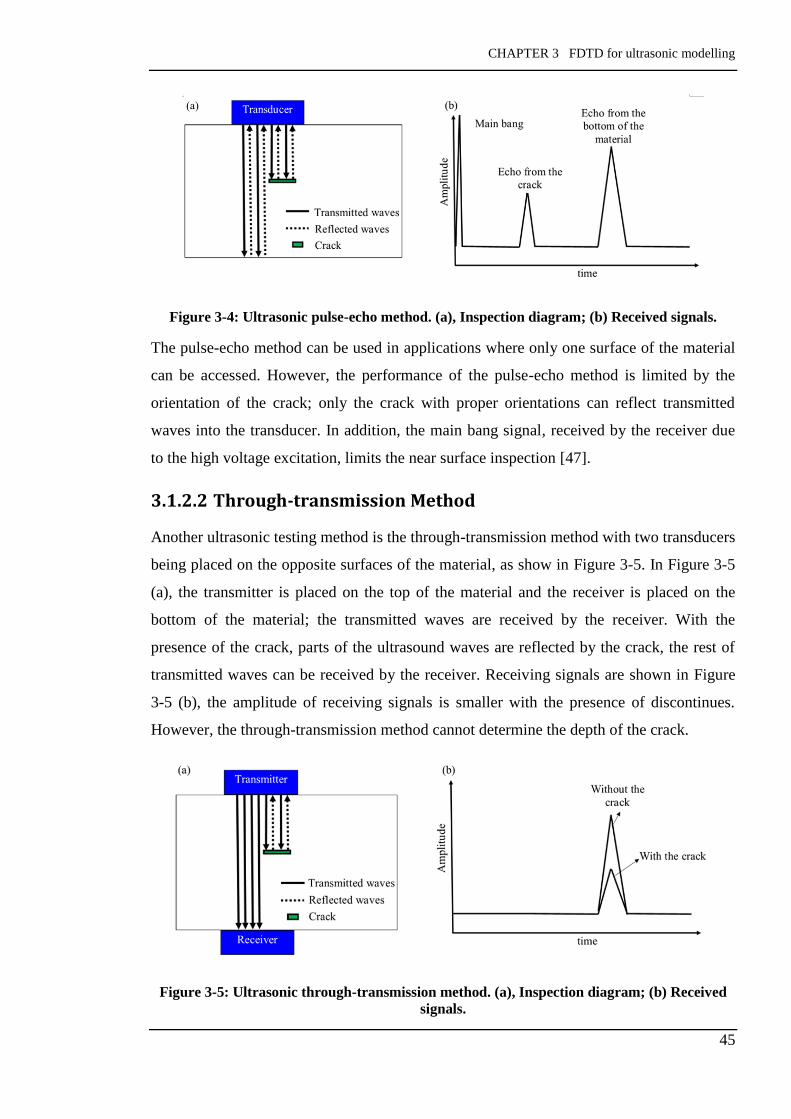
CHAPTER 3 FDTD for ultrasonic modelling
45
Figure 3-4: Ultrasonic pulse-echo method. (a), Inspection diagram; (b) Received signals.
The pulse-echo method can be used in applications where only one surface of the material
can be accessed. However, the performance of the pulse-echo method is limited by the
orientation of the crack; only the crack with proper orientations can reflect transmitted
waves into the transducer. In addition, the main bang signal, received by the receiver due
to the high voltage excitation, limits the near surface inspection [47].
3.1.2.2 Through-transmission Method
Another ultrasonic testing method is the through-transmission method with two transducers
being placed on the opposite surfaces of the material, as show in Figure 3-5. In Figure 3-5
(a), the transmitter is placed on the top of the material and the receiver is placed on the
bottom of the material; the transmitted waves are received by the receiver. With the
presence of the crack, parts of the ultrasound waves are reflected by the crack, the rest of
transmitted waves can be received by the receiver. Receiving signals are shown in Figure
3-5 (b), the amplitude of receiving signals is smaller with the presence of discontinues.
However, the through-transmission method cannot determine the depth of the crack.
Figure 3-5: Ultrasonic through-transmission method. (a), Inspection diagram; (b) Received
signals.
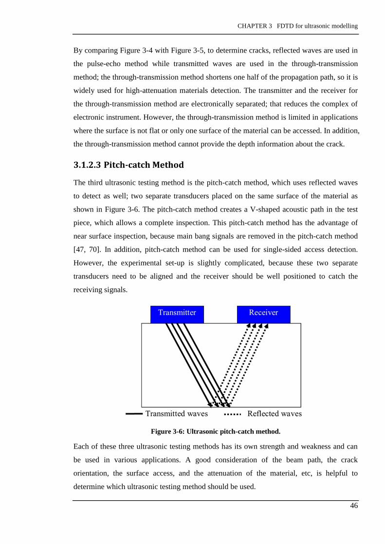
CHAPTER 3 FDTD for ultrasonic modelling
46
By comparing Figure 3-4 with Figure 3-5, to determine cracks, reflected waves are used in
the pulse-echo method while transmitted waves are used in the through-transmission
method; the through-transmission method shortens one half of the propagation path, so it is
widely used for high-attenuation materials detection. The transmitter and the receiver for
the through-transmission method are electronically separated; that reduces the complex of
electronic instrument. However, the through-transmission method is limited in applications
where the surface is not flat or only one surface of the material can be accessed. In addition,
the through-transmission method cannot provide the depth information about the crack.
3.1.2.3 Pitch-catch Method
The third ultrasonic testing method is the pitch-catch method, which uses reflected waves
to detect as well; two separate transducers placed on the same surface of the material as
shown in Figure 3-6. The pitch-catch method creates a V-shaped acoustic path in the test
piece, which allows a complete inspection. This pitch-catch method has the advantage of
near surface inspection, because main bang signals are removed in the pitch-catch method
[47, 70]. In addition, pitch-catch method can be used for single-sided access detection.
However, the experimental set-up is slightly complicated, because these two separate
transducers need to be aligned and the receiver should be well positioned to catch the
receiving signals.
Figure 3-6: Ultrasonic pitch-catch method.
Each of these three ultrasonic testing methods has its own strength and weakness and can
be used in various applications. A good consideration of the beam path, the crack
orientation, the surface access, and the attenuation of the material, etc, is helpful to
determine which ultrasonic testing method should be used.

CHAPTER 3 FDTD for ultrasonic modelling
47
3.2 FDTD Method for Ultrasonic Modelling
In section 3.1, ultrasonic phased array techniques and ultrasonic testing methods are
described. The finite-element time-domain (FDTD) method is capable of modelling
ultrasound propagation phenomena; in this section, the elastodynamic equations and the
finite-element time-domain (FDTD) are introduced.
3.2.1 Elastodynamic Equations
Elastodynamic equations are a set of partial differential equations describing how linearly
elastic material deforms and becomes internally stressed as shown in Equation 3-6 and
Equation 3-7 [71, 72].
Equation 3-6
𝜌(𝑥)𝜕𝒗𝒊𝜕𝑡
(𝑥, 𝑡) =∑𝜕𝑻𝒊𝒋
𝜕𝑥𝑗(𝑥, 𝑡)
𝑑
𝑗=1
+ 𝒇𝒊 (𝑥, 𝑡)
Equation 3-7
𝜕𝑻𝒊𝒋
𝜕𝑡(𝑥, 𝑡) =∑∑𝑐𝑖𝑗𝑘𝑙(𝑥)
𝑑
𝑖=1
𝜕𝒗𝑘𝜕𝑥𝑙
𝑑
𝑗=1
(𝑥, 𝑡)
where 𝜌 is the mass density of the material and 𝑐𝑖𝑗𝑘𝑙 is a 4th-order stiffness tensor of the
material, 𝒇𝒊(𝑥, 𝑡) is the force source; 𝒗𝒊(𝑥, 𝑡) is the velocity component and 𝑻𝒊𝒋(𝑥, 𝑡) is the
stress tensor component.
Equation 3-6 is Newton’s Second Law: when a force is applied to a testing sample, stress
and deformation are generated, as well as the particle displacement. The force per unit
volume on the infinitesimal of sample, 𝒇, is,
Equation 3-8
𝒇 = 𝑚 ∙ 𝒂 = 𝜌 ∙𝜕𝒗
𝜕𝑡
where 𝑚 is the mass of the infinitesimal, 𝒂 is the acceleration of infinitesimal; 𝒇 contains
the force source per unit volume (𝒇𝒊) and the internal stress term (𝒇𝒊𝒔). The internal stress
term can be described as,

CHAPTER 3 FDTD for ultrasonic modelling
48
Equation 3-9
𝒇𝒊𝒔 = 𝜕𝑻
𝜕𝑥
where 𝑻 is a 2nd-order stress tensor.
Equation 3-7 describes the relationship of the stress tensor rate and the strain tensor rate
based on Hooke’s Law; Hooke’s Law is shown in Equation 3-10.
Equation 3-10
𝑻 = 𝑐 ∙ 𝜺 = 𝑐 ∙𝜕𝒖
𝜕𝑥
where 𝑻 and 𝜺 are the 2nd-order stress tensor and 2nd-order strain tensor respectively, 𝒖 is
the displacement of the infinitesimal. The relationship between the stress tensor rate and
the strain tensor rate is,
Equation 3-11
𝜕𝑻
𝜕𝑡= 𝑐 ∙
𝜕𝒖
𝜕𝑥𝜕𝑡= 𝑐 ∙
𝜕𝒗
𝜕𝑥
3.2.2 The Finite-difference time-domain (FDTD) Method
From Equation 3-6 and Equation 3-7, the parameters 𝒗𝒊 and 𝑻𝒊𝒋 are to be calculated; the
finite-element time-domain (FDTD) method is a reliable method to solve these partial
differential equations. The finite-element time-domain (FDTD) method employs partial
derivatives approximations, which including forward difference approximations, backward
difference approximations, and central difference approximations; in this work, central
difference approximations (as shown in Equation 3-12) are used.
Equation 3-12
𝜕𝑓(𝑎)
𝜕𝑎≈𝑓 (𝑎 +
∆𝑎2 ) − 𝑓 (𝑎 −
∆𝑎2 )
∆𝑎
Applying Equation 3-12 to Equation 3-6 and Equation 3-7, both the time derivatives 𝜕𝒗𝒊
𝜕t,
𝜕𝑻𝒊𝒋
𝜕t and the spatial derivatives
𝜕𝑻𝒊𝒋
𝜕𝑥𝑗, 𝜕𝒗𝑘
𝜕𝑥𝑙 can be approximated with a proper time step ∆𝑡 and
a proper spatial step ∆𝑥. The time step ∆𝑡 and the spatial step ∆𝑥 should be small enough
to maintain the calculation accuracy [72].

CHAPTER 3 FDTD for ultrasonic modelling
49
Typically, the spatial step ∆𝑥 should be as small as one tenth of the wavelength, 𝜆 10⁄ ; for
some simulations with a propagating distance over tens of wavelengths, the spatial step ∆𝑥
should be smaller as 𝜆 20⁄ [72]. The time step ∆𝑡 is determined by the Courant–Friedrichs–
Lewy (CFL) condition,
Equation 3-13
∆𝑡 ≤1
√𝑑∙∆𝑥
𝑣𝑚𝑎𝑥
where 𝑑 is the space dimension, e.g., 𝑑 = 2 for 2D simulations; 𝑣𝑚𝑎𝑥 is the maximum
velocity within the modelling material. The CFL condition is to choose the maximum time
step based on the spatial step, in other words, the maximum time step is limited by or
convergence to the minimum of spatial step [72, 73].
3.3 Ultrasonic Phased Array Modelling with FDTD
In this section, the finite-difference time-domain (FDTD) method is used to model
ultrasonic phased array techniques; this is a 2D simulation, and the modelling geometry is
shown in Figure 3-7 (a) and Figure 3-7 (b), where the test piece used is a steel plate. The
steel plate has a dimension of 100mm×100mm; a transducer with 8 elements is used; the
focal point is placed in the centre of the modelling geometry. Perfectly matched layer
(PML) conditions are applied to the surround of the modelling geometry to absorb
reflections. Detailed parameters are shown in Table 3-1; the pitch means the centre-to-
centre distance between two adjacent elements.
Figure 3-7: Modelling geometry for steering (a) and focusing (b).

CHAPTER 3 FDTD for ultrasonic modelling
50
Table 3-1: Parameters used for modelling steering and focusing
Test piece
(Steel plate)
Parameters
Length Height Density
100 mm 100 mm 7.8 g/cm3
Elements
Elements
number Height Length Pitch
8 0.1 mm 0.1 mm 4 mm
FDTD setup Spatial step Time step Frequency Maximum Velocity
0.1 mm 0.0119 𝜇s 2 MHz 5.9 mm/𝜇s
Boundary
conditions
Boundary type Thickness of the boundary
Perfectly matched layer (PML) 4 mm
The excitation source used is an explosive source, which is the same with the one used in
[8]. Various sources can be added, but the explosive source is easily modelled by adding
the same excitation source, such as Gaussian pulse, to T11 and T22 at the same source point.
The pulse used in this work is a Gaussian-modulated sinusoidal wave, which can be
expressed as [74],
Equation 3-14
𝑠(𝑡) = 𝐴𝑒−𝛽(𝑡−𝑡0)2∙ 𝑠𝑖𝑛 [2𝜋𝑓(𝑡 − 𝑡0)]
where 𝐴 is the amplitude, 𝑡 is the excitation duration, 𝑡0 determines the time delay of the
waveform, 𝛽 is the bandwidth factor, 𝑓 is the central frequency.
Gaussian-modulated sinusoidal wave has various advantages over the pure sine wave, 1),
better time and frequency localization, in other words, signal arriving times of the
Gaussian-modulated sinusoidal wave are more clearly in the time domain and the energy
is more concentrated on the central frequency in the frequency domain as shown in Figure
3-8 and Figure 3-9 [75]; 2), the Gaussian-modulated sinusoidal wave covers a range of
frequencies of interest, and the waveform can be adjusted by changing the central
frequency and the bandwidth; both of these properties provide a better simulation
environment.

CHAPTER 3 FDTD for ultrasonic modelling
51
Figure 3-8: Pure sine wave; (a) the time
domain signal of the pure sine wave; (b)
the magnitude of the pure sine wave’s
Fourier transform [75].
Figure 3-9: Gaussian-modulated sine wave;
(a) the time domain signal of the Gaussian-
modulated sine wave; (b) the magnitude of
the Gaussian-modulated sine wave’s
Fourier transform [75].
The firing time’s calculation of the steering technique has been described in section 3.1.1;
firing elements with prescribed calculated times, the wavefront can be controlled to steer at
an arbitrary angle, as shown in Figure 3-10. Because perfectly matched layer (PML)
conditions are applied to the boundary of the simulated geometry, no reflections are
generated from the boundary. From Figure 3-10, a transducer with multiple elements is
capable of sweeping beam without mechanically moving the transducer, so it enlarges the
inspecting area and improving the scanning time.

CHAPTER 3 FDTD for ultrasonic modelling
52
Figure 3-10: Steering techniques: firing elements at prescribed calculated times, the
wavefront is steered at 00, 300, 600, 900 respectively.
Figure 3-11 describes the focusing behaviour; after firing elements at prescribed times, the
wavefront is becoming smaller before arriving at the prescribed focal point and becoming
larger when beyond the focal point. Because focusing allows the beam shape to be
controlled and the acoustic energy to be concentrated on the expected defect location, it
further optimizes the detection capability.

CHAPTER 3 FDTD for ultrasonic modelling
53
Figure 3-11: Focusing techniques: the wavefront is focused at the prescribed focal point.
Both steering and focusing are valuable for ultrasonic inspections; in order to further study
the properties of steering and focusing, radiation pattern is introduced in section 3.4;
section 3.5 combines radiation pattern, near field and far field together to perform
quantitative analysis of beam properties.
3.4 Novel Radiation Pattern with Hilbert Transformation
Radiation pattern defines the strength or the power of the ultrasound waves generated by
the transducer; in other words, the strength of the velocity field or the strength of the stress
field within the test piece forms the radiation pattern. Radiation pattern is the foundation of
studying beam features and further facilitates the optimal design of the transducer. In this
work, a novel radiation pattern with Hilbert transformation is proposed.
3.4.1 Hilbert Transformation
Hilbert transformation, which can extend the real signal of time-domain into the analytical
signal of the same domain, is used to return the envelope of a time series signal, as shown
in Equation 3-15, Equation 3-16 and Equation 3-17.
Equation 3-15
ℎ(𝑡) = 𝑓(𝑡) ∗1
𝜋𝑡
Equation 3-16
𝑧(𝑡) = 𝑓(𝑡) + 𝑗ℎ(𝑡)
Equation 3-17
𝑒(𝑡) = √𝑓(𝑡)2 + ℎ(𝑡)2

CHAPTER 3 FDTD for ultrasonic modelling
54
where 𝑓(𝑡) is the original time series signal, ℎ(𝑡) is the signal with Hilbert transformation,
𝑧(𝑡) is the analytical signal, and 𝑒(𝑡) is the envelope of the analytical signal 𝑧(𝑡).
As described in section 3.1.2, the depth of the defect can be deducted from the travelling
time of echoes, so how to get the arriving time of echoes is paramount. The maximum
amplitude of the time series signal indicates the arrival time of the signal, as shown in
Figure 3-12(a). In order to further improve the arrival time identification, Hilbert
transformation is employed; the envelope of the signal, returned by Hilbert transformation,
results in the signal arrival times can be identified more clearly as shown in Figure 3-12(b).
It can be seen using the Hilbert transformation to return the analytical signal is similar to
the process of amplitude modulation.
Figure 3-12: Signals to indicate the arrival times of ultrasound waves.
3.4.2 Novel Radiation Pattern with the Hilbert Transformation
Traditional radiation pattern for ultrasonic phased arrays is obtained with combining the
analytical method and the numerical method, that is, the analytical method for the pressure
distribution of focusing and the numerical method for the pressure distribution of steering
[76, 77].
In this work, a wholly numerical model is built; the finite-difference time domain (FDTD)
method and the Hilbert Transformation are combined together to produce the radiation
pattern. The finite-difference time domain (FDTD) method is used to solve the
elastodynamic equations and generate the velocity fields or pressure fields; Hilbert
transformation is used to obtain the envelope fields. Taking the steering model used in
Figure 3-7 (a) as an example, the modelling geometry is 100 mm×100 mm and the spatial
step is 0.1 mm, hence there are 1001×1001 spatial points in this model. With FDTD

CHAPTER 3 FDTD for ultrasonic modelling
55
calculation, each spatial point on the modelling geometry has a time series signal related to
the velocity or the pressure. The maximum value of the envelope of each time series signal
forms a 1001×1001 envelope fields, which is referred as the radiation pattern in this work.
The model used to study radiation pattern is the one used in the steering modelling with a
steering angle 300 (Figure 3-10); by combining the finite-difference time-domain (FDTD)
method and Hilbert transformation, the radiation pattern of the steering with a steering
angle 300 is shown in Figure 3-13 (a). The radiation pattern indicates the strength of
ultrasound waves; from Figure 3-13 (a), the beam has the largest strength along this
prescribed steering angle 300.
Figure 3-13: (a), Radiation pattern for the beam steered at 300; (b), radiation pattern for
studying beam features.
In order to quantitatively analyse the beam features, beam directivity and field distribution
along the steering angle are introduced. Beam directivity is, at a specific distance from the
centre of the sensor, the velocity field distribution; as shown in Figure 3-13 (b), beam
directivity is the velocity distribution along the white arc. Field distribution along the
steering angle is the velocity distribution along the steering angle; in Figure 3-13 (b), field
distribution along the steering angle is the velocity distribution along the red line.
Actually, the beam features are strongly related to the near field and the far field [76, 77].
Next, the beam properties of steering and focusing behaviours in the near field and in the
far field are studied respectively in section 3.5.
3.5 Near Field and Far Field Modelling
The near field and the far field are two different regions of ultrasound waves transition,
which are defined based on Equation 3-18 [69, 78].
(a) (b)

CHAPTER 3 FDTD for ultrasonic modelling
56
Equation 3-18
𝑇 =𝐴2
4𝜆
where 𝐴 is the overall length of the ultrasonic array, and 𝜆 is the wavelength of the
ultrasound wave. The near field means the distance from the centre of the ultrasonic array
is smaller than T, while the far field is larger than 𝑇.
A model is built to study the focusing and the steering properties in the near field and in
the far field; detailed parameters are shown in Table 3-2. The operational frequency used is
2 MHz and the velocity within the steel plate is 5.9 mm/𝜇s, so the wavelength λ is close to
3 mm. The spatial step chose is 0.1 mm, which approximately equals to λ/30; The pitch
(centre-to-centre distance) of two adjacent elements equals to λ/2 in order to provide a
sharper main lobe [11]. Based on Equation 3-18, T is calculated, which approximately
equals to 43.3 mm; the near field is the zone with a radial distance from the centre of the
array smaller than 43.3 mm, while the far field is beyond that zone.
Table 3-2: Detailed parameters used for near and far fields modelling.
Test piece
(Steel plate)
Parameters
Length Height Density
200 mm 200 mm 7.8 g/cm3
Elements
Elements
number Height Length Pitch
16 0.1 mm 0.5 mm 1.5 mm
FDTD setup Spatial step Time step Frequency Maximum Velocity
0.1 mm 0.0119 𝜇s 2 MHz 5.9 mm/𝜇s
Boundary
conditions
Boundary type Thickness of the boundary
Perfectly matched layer (PML) 4 mm
3.5.1 Near Field Analysis
3.5.1.1 Focusing
For the focusing behaviour, by firing elements at different times, the beam can be focused
at a specific point, which is named the focal point; the distance between the centre of the
element and the focal point is called the focal length. There are two parameters related to
the focusing beam; as shown Figure 3-14, r denotes the focal length and θ denotes the

CHAPTER 3 FDTD for ultrasonic modelling
57
steering angle. By controlling the focal length to a specific value which is smaller than T
(Equation 3-18), the focusing behaviour in the near field can be analysed.
Figure 3-14: The description of the focal length and the steering angle.
In this model, the near field is the zone with a focal length smaller than 43.3 mm
(calculated from parameters listed in Table 3-2). Any focal points with a distance from the
centre of the elements array smaller than 43.3 mm can be chosen to study the focusing
behaviour in the near field; here a focal point with the focal length of 40 mm and the
steering angle of 300 is chosen; the radiation pattern of the focusing behaviour in the near
field is shown in Figure 3-15. From this image, the beam is focused to the specific focal
zone; the acoustic intensity of the focal zone is largest.
Figure 3-15: The radiation pattern of the focusing behaviour in the near field.

CHAPTER 3 FDTD for ultrasonic modelling
58
Beam features of the focusing behaviour within the near field are shown in Figure 16. In
Figure 3-16(a), the focusing behaviour shows a good directivity with a narrow main lobe;
the maximum magnitude occurs at the simulated steering angle 300, which is consistent
with the prescribed steering angle. Figure 3-16(b) shows the field distribution along the
steering angle 300; the maximum magnitude occurs at a focal length of 32.9 mm instead of
the prescribed focal length 40mm. This observation is consistent with the analytical results
from [69], who claims this phenomenon is due to the effect of diffraction.
Figure 3-16: Beam features of focusing within the near filed. (a), Beam directivity of the
focusing behaviour; (b) Field distribution along the steering angle of the focusing behaviour.
3.5.1.2 Steering
For the steering behaviour, by firing elements with different delays, the beam can be
steered to a specific angle. In order to compare beam features of steering with them of
focusing within the near field, the same steering angle, 300, is chosen to study the steering
behaviour. The radiation pattern of the steering behaviour with the steering angle 300 is
shown in Figure 3-17. From this image, the acoustical intensity is distributed along the
steering angle; it is hard to tell where the maximum acoustical intensity occurs.
(a) (b)
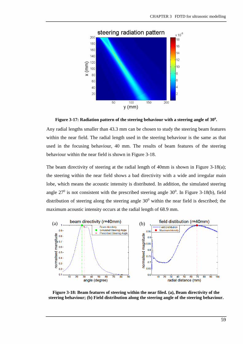
CHAPTER 3 FDTD for ultrasonic modelling
59
Figure 3-17: Radiation pattern of the steering behaviour with a steering angle of 300.
Any radial lengths smaller than 43.3 mm can be chosen to study the steering beam features
within the near field. The radial length used in the steering behaviour is the same as that
used in the focusing behaviour, 40 mm. The results of beam features of the steering
behaviour within the near field is shown in Figure 3-18.
The beam directivity of steering at the radial length of 40mm is shown in Figure 3-18(a);
the steering within the near field shows a bad directivity with a wide and irregular main
lobe, which means the acoustic intensity is distributed. In addition, the simulated steering
angle 270 is not consistent with the prescribed steering angle 300. In Figure 3-18(b), field
distribution of steering along the steering angle 300 within the near field is described; the
maximum acoustic intensity occurs at the radial length of 68.9 mm.
Figure 3-18: Beam features of steering within the near filed. (a), Beam directivity of the
steering behaviour; (b) Field distribution along the steering angle of the steering behaviour.
(a) (b)

CHAPTER 3 FDTD for ultrasonic modelling
60
3.5.1.3 Comparison and Discussion
Comparing the beam directivity between the focusing and the steering within the near field,
as shown in Figure 3-16(a) and Figure 3-18(a) respectively, the focusing behaviour within
the near field provides a better directivity over the steering behaviour within the near field;
the acoustic energy is more concentrated along the steering angle with the focusing
behaviour.
Comparing the field distribution between the focusing and the steering within the near field,
as shown in Figure 3-16(b) and Figure 3-18(b) respectively, the acoustic intensity of the
focusing is more concentrated than that of the steering. Due to the good beam directivity
and concentrated acoustic intensity in the specific area, focusing is normally employed for
near-field inspections.
One point should be noted is that the maximum acoustic intensity of the focusing does not
occur at the prescribed focal length, as shown in Figure 3-16(b); the simulated focal
length, 32.9 mm, is 17.75% ahead of the prescribed focal length 40mm. However, the
prescribed focal length shows the optimal beam directivity as shown in Figure 3-19: only
for the prescribed focal length of 40 mm, the simulated steering angle is consistent with the
prescribed steering angle. Away from this radial distance, the beam directivity has a wider
main lobe (Figure 3-19(a)).
(a) (b)

CHAPTER 3 FDTD for ultrasonic modelling
61
Figure 3-19: The beam directivity of the focusing behaviour at different radial lengths.
3.5.2 Far Field Analysis
3.5.2.1 Focusing
The model used for studying the focusing behaviour in the far field is the same with the
one used for the focusing behaviour within the near field, apart from one difference, that is,
the focal point is placed in the far field. Any focal points beyond the near field can be
chosen to study the focusing behaviour in the far field, here the focal point has a focal
depth of 150 mm and the steering angle is 300 is chosen. The radiation pattern of the
focusing behaviour in the far field is shown in Figure 3-20; the acoustic intensity is not
clearly focused on a specific zone in the far field.
Figure 3-20: Radiation pattern of the focusing behaviour in the far field.
(c) (d)

CHAPTER 3 FDTD for ultrasonic modelling
62
Figure 3-21 (a) depicts the beam directivity of the focusing behaviour in the far field; away
from the near field, focusing still shows a good directivity with a narrow main lobe; the
simulated steering angle is matched with the prescribed steering angle. However, the
maximum acoustic intensity occurs at a radial length of 55.8 mm instead of 150 mm as
shown in Figure 3-21 (b). It means the beam does not concentrate on the expected location
when the focal point is placed in the far field. Unlikely with the focusing technique in the
near field, the focusing technique in the far field lose the advantage of the concentrated
acoustic intensity.
Figure 3-21: Beam features of focusing in the far field: (a) beam directivity at a focal length
of 150 mm, (b) field distribution along the steering angle 300.
3.5.2.2 Steering
The beam features of the steering behaviour within the near field has been studied in
section 3.5.1.2; the model and the radiation pattern used to study the steering behaviour in
the far field are exact the same as ones used in the near field.
Any radial lengths larger than the near field can be picked to study the beam features of the
steering behaviour; in order to compare the steering and the focusing in the far field, the
same radial length, 150 mm, is chosen; Figure 3-22 depicts the beam features of steering in
the far field.
The beam directivity of the steering behaviour in the far field, as shown in Figure 3-22(a),
shows a better directivity than that in the near field; the acoustic intensity in the far field is
mainly along the prescribed steering angle 300. The simulated steering angle is matched
with the prescribed steering angle 300. Figure 3-22(b) shows the field distribution along the
steering angle, the maximum acoustic intensity occurs at a radial length of 68.9 mm.
(a) (b)

CHAPTER 3 FDTD for ultrasonic modelling
63
Figure 3-22: Beam features of steering in the far field: (a) beam directivity at a radial length
of 150 mm, (b) field distribution along the steering angle 300.
3.5.2.3 Comparison and Discussion
Comparing the beam directivity between the focusing and the steering in the far field, as
shown in Figure 3-21(a) and Figure 3-22(a) respectively, both the focusing and the steering
provide a good beam directivity with a narrow main lobe.
Comparing the field distribution along the steering angle, as shown in Figure 3-21(b) and
Figure 3-22(b) respectively, the focusing does not concentrated the beam to the expected
area, and the field distribution of the focusing in the far field is close to that of steering in
the far field; it indicates, in the far field, the field distribution of focusing is convergence to
that of steering.
Combining the beam directivity and field distribution along the steering angle, steering is
sufficiently reliable in the far field. In addition, because steering needs less modelling time,
such as less firing time calculation and less scanning points, the steering provides more
advantages than focusing in the far field [69]. Therefore, the steering technique is normally
used for far-field inspections.
3.5.3 Conclusions of Section 3.5
For near-field inspections, the focusing technique provides some attractive features over
the steering technique, such as a good beam directivity and a concentrated acoustic
intensity in the expected area; so focusing is normally employed for near-field inspections.
Especially, for applications that possible defect locations in the near field are known, the
focusing technique is a reliable method optimizing the detection capability. It is important
to note that the beam is focusing at a radial length slightly smaller than the focal length,
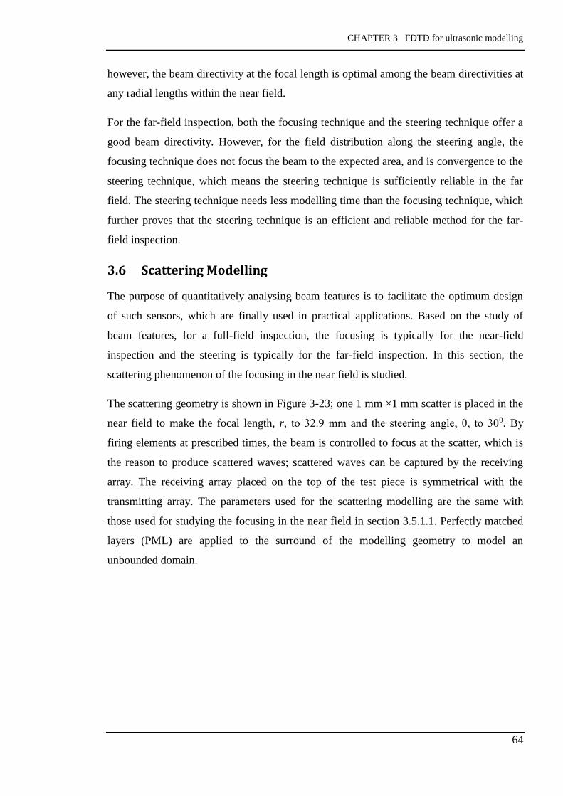
CHAPTER 3 FDTD for ultrasonic modelling
64
however, the beam directivity at the focal length is optimal among the beam directivities at
any radial lengths within the near field.
For the far-field inspection, both the focusing technique and the steering technique offer a
good beam directivity. However, for the field distribution along the steering angle, the
focusing technique does not focus the beam to the expected area, and is convergence to the
steering technique, which means the steering technique is sufficiently reliable in the far
field. The steering technique needs less modelling time than the focusing technique, which
further proves that the steering technique is an efficient and reliable method for the far-
field inspection.
3.6 Scattering Modelling
The purpose of quantitatively analysing beam features is to facilitate the optimum design
of such sensors, which are finally used in practical applications. Based on the study of
beam features, for a full-field inspection, the focusing is typically for the near-field
inspection and the steering is typically for the far-field inspection. In this section, the
scattering phenomenon of the focusing in the near field is studied.
The scattering geometry is shown in Figure 3-23; one 1 mm ×1 mm scatter is placed in the
near field to make the focal length, r, to 32.9 mm and the steering angle, θ, to 300. By
firing elements at prescribed times, the beam is controlled to focus at the scatter, which is
the reason to produce scattered waves; scattered waves can be captured by the receiving
array. The receiving array placed on the top of the test piece is symmetrical with the
transmitting array. The parameters used for the scattering modelling are the same with
those used for studying the focusing in the near field in section 3.5.1.1. Perfectly matched
layers (PML) are applied to the surround of the modelling geometry to model an
unbounded domain.

CHAPTER 3 FDTD for ultrasonic modelling
65
Figure 3-23: The geometry of scattering modelling.
The wave propagation at different times are shown in Figure 3-24; because the perfectly
matched layer is applied to the surround of the modelling geometry, there is no reflections
from boundaries. Before arriving at the scatter, the wavefront is becoming smaller, as
shown in Figure 3-24(a) and Figure 3-24(b). Ultrasound waves are scattered when
encounter the scatter, which produces the scattered longitudinal waves and the scattered
shear waves (Figure 3-24(c)). The velocity of the longitudinal wave is larger than that of
the shear wave, so longitudinal waves propagate ahead of shear waves; as shown in Figure
3-24(d), two circles are generated due to the scatter, the outside circle is the longitudinal
wave and the inside circle is the shear wave.
(a) (b)

CHAPTER 3 FDTD for ultrasonic modelling
66
Figure 3-24: Wave propagation of the scattering modelling at different times.
Both the scattered longitudinal waves and the scattered shear waves can be received by the
receiving array. Each element on this receiving array can capture the scattered signal; the
totally received signal is the sum of the scattered signal received by each element. The
receiving signal is shown in Figure 3-25; the first arrival signals are the directly transmitted
waves generated from the transmitted array (Figure 3-25(a)). The followed signals, as
shown in Figure 3-25(b) and Figure 3-25(c) respectively, are scattered longitudinal waves
and scattered shear waves.
Figure 3-25: The received signals from the receiving array. (a), directly transmitted signals;
(b), the scattered longitudinal waves; (c), the scattered shear waves.
3.7 Conclusions
Steering and focusing are two widely used phased array techniques; steering enlarges the
inspection area and focusing optimizes the detection capability. The FDTD solver,
SimSonic, was further developed / adapted by the author for simulating ultrasound waves’
behaviours; Gaussian-modulated sinusoidal wave, which provides a better simulation
(c) (d)
(a)
(b) (c)

CHAPTER 3 FDTD for ultrasonic modelling
67
environment, was used as the excitation source. The combination of the finite-difference
time-domain (FDTD) method and Hilbert transformation is capable of generating the
radiation pattern, which lays a substantial foundation for studying the beam features of
steering and focusing.
Based on the modelling results, a number of important conclusions can be drawn; the
focusing technique has some advantages in the near field, such as a concentrated acoustic
intensity and a good beam directivity; the steering technique has advantages in the far field,
such as less modelling time and a good beam directivity. For a full-field inspection, the
focusing technique is used for the near-field inspection while the steering technique is used
for the far-field inspection. Finally, the scattering phenomenon is simulated by the finite-
difference time-domain (FDTD) method. Both the directly transmitted signals and the
scattered signals can be captured by the receiving array.
All of the work included in this chapter verified the ability of FDTD to model ultrasound
waves’ propagation; this lays a foundation for the EMATs modelling, which contains
electromagnetic and ultrasonic models; the EMATs modelling based on FDTD and the
analytical method is introduced in Chapter 4.

CHAPTER4 Development and validation of a novel method for modelling meander-line-coil EMATs
operated on Lorentz force mechanism
68
Chapter 4 Development and Validation of A Novel Method
for Modelling Meander-line-coil EMATs Operated
on Lorentz Force Mechanism
In this chapter, a novel modelling method for simulating electromagnetic acoustic
transducers (EMATs) operated on Lorentz force mechanism to generate Rayleigh waves is
proposed. This novel modelling method, focusing on the vertical plane of the material,
combines the analytical method and the finite-difference time-domain (FDTD) method
together. Based on this proposed modelling method, several behaviours of Rayleigh waves,
including the bidirectional propagation (Section 4.3), the scattering behaviour (Section 4.7)
and the unidirectional propagation (Section 4.8), are studied. Related experiments were
conducted to validate the capability of this novel modelling method. The novel modelling
method presented in this chapter and related chapters haven been published in or accepted
by Ultrasonics, Journal of Sensors and International Journal of Applied Electromagnetics
and Mechanics [10, 13, 14].
4.1 Introduction
The simulation of EMATs operated on the Lorentz mechanism is normally divided into
two parts, the electromagnetic (EM) simulation and the ultrasonic (US) simulation. The
link between the EM simulation and the US simulation is the Lorentz force density. In this
work, the EM simulation is performed with an analytical method, which is adapted from
classic Dodd and Deeds solutions which were originally intended for the circular coil. The
US simulation is accomplished by the finite-difference time-domain (FDTD) method,
which has been described in Chapter 3.
4.1.1 Modelling Geometry
The test piece used is a stainless steel plate with a dimension of 600 mm×600 mm×25 mm,
the permanent magnet used is NdFeB35 whose size is 60 mm×60 mm×25 mm. The
conductivity and the permittivity of the stainless steel is 1.1×10⁶ Siemens/m and 1.26×10⁻⁶
H/m respectively. The frequency used is 500 kHz, thus the skin depth calculated is 0.679
mm. The velocity of the longitudinal waves, the shear waves and the Rayleigh waves
within the stainless steel is 5.9 mm/µs, 3.25 mm/µs and 3.033 mm/µs respectively [39].
The coil used is a meander-line-coil carrying an alternating current (Figure 4-1); the

CHAPTER4 Development and validation of a novel method for modelling meander-line-coil EMATs
operated on Lorentz force mechanism
69
effective length of the meander-line-coil (L) is 40 mm; the width of each wire of the
meander-line-coil (w) is 0.4 mm; the height of the meander-line-coil is 0.035 mm, and the
centre-to-centre distance between two adjacent wires of the meander-line-coil (s) is 3.033
mm, which is half of the Rayleigh waves’ wavelength to achieve the constructive
interference.
Figure 4-1: The configuration of a typical meander-line-coil EMAT.
4.2 EMAT-EM Modelling
The electromagnetic simulation is accomplished with an analytical method adapted from
the classic Dodd and Deeds solution, which was originally used for circular coils [79].
Firstly, the strategy of adapting the analytical solution for a straight wire is proposed.
Finite element method (FEM) is employed to validate the adapted analytical solution. Next,
the analytical EM simulation for the meander-line-coil EMAT is described; the distribution
of Lorentz force density is obtained.
4.2.1 Classic Dodd and Deeds Solutions
The Dodd and Deeds solution for the eddy current phenomenon is employed in this work,
because the analytical solution proposed by Dodd and Deeds has a high accuracy and a
minimum model difference between the model built by Dodd and Deeds and the author.
The eddy current calculation is governed by Equation 4-1, Equation 4-2 and Equation 4-3
[79],
Equation 4-1
𝛻2𝑨 = −𝜇𝑰 + 𝜇𝜎𝜕𝑨
𝜕𝑡+ 𝜇𝜀
𝜕2𝑨
𝜕𝑡2+ 𝜇𝛻(
1
𝜇) × (𝛻 × 𝑨)

CHAPTER4 Development and validation of a novel method for modelling meander-line-coil EMATs
operated on Lorentz force mechanism
70
Equation 4-2
𝑬 = −𝑗𝜔𝑨
Equation 4-3
𝑱 = 𝜎𝑬
where 𝑨 is the vector potential generated by the coil carrying a current density 𝑰; µ, σ, and
ε are the permeability, the conductivity and the permittivity of the test piece respectively. 𝑬
is the induced electric field, and 𝑱 is the induced eddy current density.
Based on Equation 4-1, Equation 4-2 and Equation 4-3, for eddy current calculation, the
fundamental step is to calculate the vector potential. Dodd and Deeds built a model with a
rectangular cross-sectional coil placed above a two-layered conductor with an infinite
length (Figure 4-2); the length “R” as shown in Figure 4-2 is the length of the conductor to
be calculated and shown; the model is axial symmetrical along the 𝑥 axis and the direction
of the AC current is anti-clockwise. Equation 4-1 is a full wave equation; with the
quasistatic approximation, the final solution to the vector potential within Layer 1 is shown
in Equation 4-4, Equation 4-5 and Equation 4-6.
Figure 4-2: A model built by Dodd and Deeds [79].
Equation 4-4
𝑨(𝑟, 𝑥) = 𝜇0𝑰∫1
𝑎3(∫ 𝛾𝐽1(𝛾)𝑑𝛾) 𝐽1(𝑎𝑟)
𝑎𝑟2
𝑎𝑟1
(𝑒−𝑎𝑙∞
0
− 𝑒−𝑎(𝑙+ℎ))𝑎(𝑎1 + 𝑎2)𝑒
(2𝑎1𝐻1)𝑒(2𝑎1𝑥) + 𝑎(𝑎1 − 𝑎2)𝑒(−𝑎1𝑥)
(𝑎 − 𝑎1)(𝑎1 − 𝑎2) + (𝑎 + 𝑎1)(𝑎1 + 𝑎2)𝑒(2𝑎1𝐻1)𝑑𝑎

CHAPTER4 Development and validation of a novel method for modelling meander-line-coil EMATs
operated on Lorentz force mechanism
71
Equation 4-5
𝑎1 = √𝑎2 + 𝑗𝜔𝜇1𝜎1
Equation 4-6
𝑎2 = √𝑎2 + 𝑗𝜔𝜇2𝜎2
Where µ0, µ1, and µ2 are the permeability of air, Layer 1 and Layer 2 respectively; σ1 and
σ2 are the conductivity of Layer 1 and Layer 2 respectively. Assuming the conductor only
has one layer, that is, the material property of Layer 1 and Layer 2 are exactly the same
(Figure 4-3); the final solution of the vector potential within the conductor with only one
layer can be simplified, as shown in Equation 4-7 and Equation 4-8.
Figure 4-3: Geometry for the conductor with only one layer.
Equation 4-7
𝐀(𝑟, 𝑥) = 𝜇0𝐈 ∫1
𝑎2(∫ 𝛾𝐽1(𝛾)𝑑𝛾) 𝐽1(𝑎𝑟)
𝑎𝑟2
𝑎𝑟1
(𝑒−𝑎𝑙 − 𝑒−𝑎(𝑙+ℎ))𝑒(2𝑎1𝑥)
(𝑎 + 𝑎1)𝑑𝑎
∞
0
Equation 4-8
𝑎1 = √𝑎2 + 𝑗𝜔𝜇1𝜎1
where 𝐀(𝑟, 𝑥) is the vector potential within the conductor, 𝜇0 is the permeability of air, 𝐈 is
the applied current density, 𝛾 and 𝑎 are the integration variables, 𝑟1 and 𝑟2 are the inside
radius and outside radius of the coil respectively, 𝐽1(𝛾) and 𝐽1(𝑎𝑟) are the first kind Bessel
functions, 𝑙 is the lift-off, ℎ is the height of the coil, 𝜇1 and 𝜎1 are the permeability and
conductivity of the conductor respectively, and 𝜔 is the angular frequency.

CHAPTER4 Development and validation of a novel method for modelling meander-line-coil EMATs
operated on Lorentz force mechanism
72
A model is built to study the vector potential distribution on the basis of the analytical
solutions proposed by Dodd and Deeds; detailed parameters used for this modelling are
shown in Table 4-1. The test piece used is a stainless steel plate with a circular coil placed
above the test piece; the frequency used is 10 kHz. The software used to build this model is
Matlab; for the integration, a limit inferior of 1×10⁻⁹ and a limit superior of 5000 are used;
the computer used for computation is with a Random Access Memory of 8 GB and with a
dual Intel Core i5-3570 with a speed of 3.4 GHz; the computation time for this model is
roughly 20 minutes.
Table 4-1: Detailed parameters used for studying analytical solutions proposed by Dodd and
Deeds.
The distribution of the magnitude of the vector potential within the conductor is shown in
Figure 4-4, where the vector potential is concentrated on the near surface of the conductor
and under the circular coil; the unit of the vector potential is Tm. The skin depth calculated
is 4.8 mm, beyond of which the vector potential significantly decreases.
Figure 4-4: For a circular coil, the distribution of the magnitude of the vector potential
within the conductor.
Test piece
(Stainless steel
plate)
Parameters
Length (R) Height (H) Permeability (𝝁𝟏) Conductivity (𝝈𝟏)
5 mm 10 mm 1.26×10⁻⁶ H/m 1.1×10⁶ Siemens/m
Coil used
(Circular coil)
Parameters
Inside Radius (𝒓𝟏) Outside Radius (𝒓𝟐) Mean Radius
(𝒓𝟏 + 𝒓𝟐)/2 Applied Current Density(I)
2.45 mm 2.55 mm 2.5 mm 1 A/m2
Frequency Lift-off Height (h) Air permeability (μ0)
10 kHz 1 mm 1 mm 1.257×10⁻⁶ H/m

CHAPTER4 Development and validation of a novel method for modelling meander-line-coil EMATs
operated on Lorentz force mechanism
73
Figure 4-5 shows the distribution of the magnitude of the vector potential along the surface
of the conductor (𝑥=0); the green marker in this curve states that the maximum magnitude
occurs at where the circular coil is located. The curve of the vector potential distribution is
not symmetrical with the radius because the wire of a circular coil is bent instead of
straight.
Figure 4-5: For a circular coil, the vector potential distribution along the surface of the
conductor (𝒙=0).
4.2.2 Adapted Analytical Solutions for A Straight Wire
The coil used for the EMAT system is a meander-line-coil with straight wires, so the
analytical solution for a straight wire is needed. On the basis of the calculation results from
section 4.2.1, we propose a hypothesis, that is, the analytical solution for a straight wire
may be obtained by expanding the radius of the circular coil to very large. In other words,
the bent wire may be approximated to a straight wire when the radius of the circular coil is
very large, and the distribution of the vector potential should be symmetrical with the
radius.
To verify this hypothesis, an analytical model is built with the same parameters used in
Table 4-1, except that the mean radius is set to 20.05 m and the length of the stainless steel
plate is 20.1 m. With a large-radius circular coil placed above the conductor, the
distribution of the magnitude of the vector potential within the conductor is shown in
Figure 4-6; it is clearly that the vector potential is mainly concentrated within the skin
depth, which is 4.8 mm in this model; beyond the skin depth, the vector potential is very
small.

CHAPTER4 Development and validation of a novel method for modelling meander-line-coil EMATs
operated on Lorentz force mechanism
74
Figure 4-6: For a large-radius circular coil, the vector potential distribution within the
conductor.
Figure 4-7 shows, for a large-radius circular coil, the distribution of the magnitude of the
vector potential along the surface of the conductor (𝑥=0). From this image, the vector
potential is symmetrical with the radius r=20.05 m, where the straight wire is located. This
verifies the hypothesis that, when the radius of the circular coil is very large, the bent wire
of the circular coil can be approximated to a straight wire, and the distribution of the
magnitude of the vector potential is symmetrical with the radius.
Figure 4-7: For a large-radius circular coil, the vector potential along the surface of the
conductor (𝒙=0).
4.2.3 Validation and Comparison with FEM
In order to analyse the accuracy of the adapted analytical solutions, the finite element
method (FEM) is employed to compare the results between the analytical and the
numerical methods. Maxwell Ansoft based on the finite element method (FEM) is used to
solve the vector potential; the model built with Maxwell Ansoft is the same as the one built
in section 4.2.2. This is a 2D model with a rectangular cross-sectional coil located above

CHAPTER4 Development and validation of a novel method for modelling meander-line-coil EMATs
operated on Lorentz force mechanism
75
the cross-sectional stainless steel plate as shown in Figure 4-8(a); the vacuum region to be
solved is four times as larger as the stainless steel plate. The finite element method (FEM)
subdivides the large model to smaller elements, as shown in Figure 4-8(b); the mesh
quality determines the accuracy of the computed results. However, the very fine mesh /
high mesh density is limited by the capacity of the computer and requires more running
times. The computation of the FEM solver is based on minimising the energy error; in
Figure 4-9, when the elements number is beyond 20000, the energy error is as low as
0.05%, which is sufficiently accurate for the FEM computation. In this work, the mesh
number used is 20395. In section 4.2.3.1 and section 4.2.3.2, the comparison between the
analytical method and the numerical method at a low frequency and a high frequency are
described respectively.
Figure 4-8: (a), the model built with Maxwell Ansoft; (b), mesh of the model.
Figure 4-9: In FEM solver, the energy error versus the number of triangles.
Coil
Stainless steel
plate
Vacuum
(a)
(b)

CHAPTER4 Development and validation of a novel method for modelling meander-line-coil EMATs
operated on Lorentz force mechanism
76
4.2.3.1 Comparison with FEM at 10 kHz
At a frequency of 10 kHz, the magnitude of the vector potential within the conductor
(stainless steel plate) from the analytical method and from the numerical method are shown
in Figure 4-10(a) and Figure 4-10(b) respectively; the analytical and numerical methods
show a good agreement about the peak magnitude, which is close to 3.5 × 10⁻⁷ Tm. From
these images, the distribution of the vector potential based on the adapted analytical
method is smoother than that based on the finite element method.
Figure 4-10: At 10 kHz, the vector potential distribution within the stainless steel plate. (a),
the analytical method; (b) the finite element method (FEM).
The vector potential along the surface of the stainless steel plate is shown in Figure 4-11
(𝑥=0); where the distribution of the magnitude, the real part and the imaginary part of the
vector potential are shown in Figure 4-11(a), Figure 4-11(b) and Figure 4-11(c)
respectively. From these images, at 10 kHz, the adapted analytical method has a good
agreement with the finite element method (FEM). One point should be noted is, the
distribution of the imaginary part of the vector potential based on the analytical method is
more accurate than FEM because the vector potential from the FEM does not approach to
zero when it is far away from the wire.
(a)
(b)
20 20.1 20.2 20.3 20.4 20.5 20.6 20.7 20.8 20.9 21
y (m)
0
-5
x (
mm
)

CHAPTER4 Development and validation of a novel method for modelling meander-line-coil EMATs
operated on Lorentz force mechanism
77
Figure 4-11: At 10 kHz, the vector potential along the surface of the stainless steel plate. (a),
(b) and (c) denotes the magnitude, the real part, and the imaginary part of the vector
potential respectively.
4.2.3.2 Comparison with FEM at 1 MHz
In this part, the comparison between the adapted analytical method and FEM at a higher
frequency is studied; this is because EMAT normally operates at high frequencies. The
geometry used for modelling has been described in section 4.2.2; the operational frequency
used is 1 MHz. The skin depth calculated is 0.48mm, which means the vector potential
should be concentrated on the region very close to the surface of the material.
The magnitude of the vector potential within the cross-section of the stainless steel plate is
shown in Figure 4-12; as expected, the vector potential is concentrated on the surface of
the stainless steel plate due to the high frequency used. From Figure 4-12(a) and Figure
4-12(b), the range of the vector potential magnitude shows a good agreement between the
adapted method and FEM; the range of the vector potential is from 0 to 8 × 10⁻⁸ Tm.
(a) (b)
(c)

CHAPTER4 Development and validation of a novel method for modelling meander-line-coil EMATs
operated on Lorentz force mechanism
78
Figure 4-12: At 1 MHz, the vector potential distribution within the stainless steel plate. (a),
the analytical method; (b) the finite element method (FEM).
Figure 4-13: At 1 MHz, the vector potential along the surface of the stainless steel plate. (a),
(b) and (c) denotes the magnitude, the real part, and the imaginary part of the vector
potential respectively.
The vector potential along the surface of the stainless steel plate (𝑥=0) is shown in Figure
4-13, where the magnitude, the real part and the imaginary part of the vector potential are
shown in Figure 4-13(a), Figure 4-13(b) and Figure 4-13(c) respectively. From these
(a)
(b)
(a) (b)
(c)
20 20.1 20.2 20.3 20.4 20.5 20.6 20.7 20.8 20.9 21
y (m)
0
-5
x (
mm
)

CHAPTER4 Development and validation of a novel method for modelling meander-line-coil EMATs
operated on Lorentz force mechanism
79
images, the curve of the real part of the vector potential based on FEM is not smooth, that
is due to the inevitable errors produced by the numerical approximation.
4.2.3.3 Comparison at Different Lift-offs
In practical applications, the lift-off is a critical parameter that determines the
electromagnetic induction efficiency; this section compares the numerical results and the
analytical results when the sensor is placed at various lift-offs.
Figure 4-14: With various lift-offs, the distribution of the real part of the vector potential
along the surface of the stainless steel plate.
The model used is the same as the one used in section 4.2.3.2, the operational frequency is
1 MHz. The lift-off varies from 2 mm to 6 mm with a step of 2 mm; the distribution of the
real part of the vector potential based on FEM and the adapted analytical method is shown
in Figure 4-14. From these images, the adapted analytical method exhibits smoothness both
at a small lift-off (2 mm) and at a high lift-off (6 mm). On the other hand, the finite
element method (FEM) does not guarantee the calculation accuracy since the curve of the
vector potential becomes increasingly distorted with the lift-off increasing. Results show a

CHAPTER4 Development and validation of a novel method for modelling meander-line-coil EMATs
operated on Lorentz force mechanism
80
benefit of the adapted analytical solution over FEM, that is, the adapted analytical method
guarantees the accuracy even if the lift-off is large.
4.2.3.4 Conclusions of Section 4.2.3
In this study, the coil used for EMATs is a meander-line-coil contains several straight
wires, thus the electromagnetic induction solution to the straight wire is needed. Classic
Dodd and Deeds solution, which was originally for the circular coil, is adapted for the
straight wire by setting the radius of the circular coil to a large value, and results show that
the bent wire can be approximated to a straight wire. The adapted analytical solution for
the straight wire is numerically verified by the finite element method (FEM). The results
show that the adapted analytical solution is desirable for the electromagnetic induction
phenomenon calculation over the finite element method (FEM).
4.2.4 Analytical EMAT-EM Modelling
The EMAT-EM modelling is divided into two parts, one part is to calculate eddy currents
produced by the meander-line-coil and the other part is to calculate the static magnetic
field generated by the permanent magnet. The eddy current is calculated analytically with
the adapted analytical method as described in section 4.2.2; the static magnetic field is
modelled with the finite element method (FEM).
4.2.4.1 Eddy Currents Calculation
As described previously, the analytical solution to the vector potential with a straight wire
located above the stainless steel plate has been studied. For an EMAT transducer
containing a meander-line-coil, the total vector potential is the sum of the vector potential
generated by each straight wire segments in the meander coil. The model is shown in
Figure 4-15; 12 straight wire segments are placed above the stainless steel plate. Detailed
parameters for the EMAT system have been introduced in section 4.1.1; the frequency
used is 500 kHz. The meander coil has a dimension of 33.763 mm×40 mm×0.035 mm,
which is very small compared to the dimension of the stainless steel plate 600 mm×600
mm×25 mm. In order to reduce the modelling dimension and improve the modelling time,
only the 2D area 100 mm×3 mm, where the meander-line-coil has a major effect on, is
chosen to perform the EM modelling; the lift-off of the meander coil is 0.1 mm. Because
the length and the width of the straight wire used in this work is 40 mm and 0.2 mm

CHAPTER4 Development and validation of a novel method for modelling meander-line-coil EMATs
operated on Lorentz force mechanism
81
respectively, the ratio of the length to the width is 200, which means the edge effect of the
finite length straight wire can be neglected.
Figure 4-15: 2D model of the EMAT-EM simulation.
By summing all the vector potential generated by each wire segment, the total vector
potential within the x-y plane of the stainless steel plate is shown in Figure 4-16; the unit of
the vector potential is Tm. Due to the AC directions between two adjacent wires of the
meander-line-coil are opposite, the vector potential produced by two adjacent wires are
opposite as well. The frequency used is 500 kHz, which results in a skin depth of 0.679
mm, thus the vector potential is mainly concentrated on the depth smaller than 0.679 mm
as shown in Figure 4-16.
Figure 4-16: The real part of the vector potential produced by a meander-line-coil.
The eddy current distribution can be obtained based on the vector potential calculation
(Equation 4-2 and Equation 4-3); the distribution of the real part of the eddy current
generated by the meander-line-coil is shown in Figure 4-17. The eddy current is
concentrated on the subsurface of the stainless steel plate; the unit of the induced eddy
current density is ampere per square meter. From Figure 4-17, the maximum amplitude of
the eddy current occurs at the leftmost side and the rightmost side of the meander-line-coil;
this is because that the outmost wires are only affected by the fields on one side.
Figure 4-18 shows the eddy current distribution along the surface of the stainless steel plate
(x=0); this curve further confirms the observation that the value of the eddy current under
the outmost wires are largest.
Stainless steel plate
Straight wire segments

CHAPTER4 Development and validation of a novel method for modelling meander-line-coil EMATs
operated on Lorentz force mechanism
82
Figure 4-17: The real part of the induced eddy current produced by a meander-line-coil.
Figure 4-18: The eddy current distribution along the surface of the stainless steel plate (x=0).
4.2.4.2 Static Magnetic Field Calculation
The other part of the EMAT-EM modelling is to calculate the static magnetic field
generated by the permanent magnet. The permanent magnet located above the stainless
steel plate is modelled with the finite element method (FEM). The permanent magnet used
is made of NdFeB35 with a relative permeability of 1.1 and a magnetic coercivity of -
890000 ampere per meter. The dimension of the permanent magnet is 60 mm×60 mm×25
mm which is slightly smaller compared to the dimension of the stainless steel plate, 600
mm×600 mm×25 mm; the region of the stainless steel plate, 100 mm×100 mm×3 mm,
where the permanent magnet has a major effect on, is picked to study the behaviour of the
permanent magnet. In this section, only the 2D behaviour of the permanent magnet is taken
into account; the modelling geometry of the stainless steel plate is 100 mm×3 mm. The
vacuum region to be solved is two times as larger as the stainless steel plate; the mesh for
this magnetostatic modelling is shown in Figure 4-19. As mentioned before, the
computation of the FEM solver is based on minimising the energy error; as shown in
Figure 4-20, the energy error is as low as 0.1% when the elements number is beyond 2000.
In this work, the mesh number used is 3599, which is sufficiently accurate for the FEM
calculation.

CHAPTER4 Development and validation of a novel method for modelling meander-line-coil EMATs
operated on Lorentz force mechanism
83
Figure 4-19: The mesh of the static magnetic field modelling.
Figure 4-20: The relationship between the elements number and the energy error for the
static magnetic field modelling.
Figure 4-21 illustrates the vector of the magnetic flux density; from this figure, the
magnetic flux density is generated from the permanent magnet and is mainly normal to the
stainless steel plate. Under the edge of the permanent magnet, the magnetic flux density
goes obliquely even parallel to the surface of the stainless steel plate due to the edge effect.
Figure 4-21: The vector of the magnetic flux density generated by the permanent magnet.
The distribution of the magnitude of the magnetic flux density within the stainless steel
plate is shown in Figure 4-22, where the magnetic flux density is mainly concentrated
under the permanent magnet and arrives to the largest under the edge of the permanent
magnet. The magnetic flux density decays with the depth of the material increasing.
NdFeB35
Vaccum

CHAPTER4 Development and validation of a novel method for modelling meander-line-coil EMATs
operated on Lorentz force mechanism
84
Figure 4-22: The distribution of the magnitude of the magnetic flux density within the
stainless steel plate.
Because the static magnetic flux density is mainly distributed along the surface of the
stainless steel plate, the analysis of the static magnetic flux density along the surface of the
specimen is needed. Figure 4-23 presents the magnetic flux density along the surface of the
specimen (x=0); the blue curve and the red curve denote the x components and y
components of the magnetic flux density respectively. Because the permanent magnet has
a length of 60 mm, this curve further states that the largest magnetic flux density occurs
under the edge of the permanent magnet.
Figure 4-23: L The distribution of the magnetic flux density along the surface of the stainless
steel plate (x=0).
4.2.4.3 Lorentz Force Density
For the EMATs operated on the Lorentz force mechanism, the Lorentz force density is
obtained based on the calculation of the static magnetic field and the induced eddy current.
The induced eddy current and the static magnetic field are obtained in section 4.2.4.1 and
section 4.2.4.2 respectively; in this section, the distribution of the Lorentz force density is
presented.

CHAPTER4 Development and validation of a novel method for modelling meander-line-coil EMATs
operated on Lorentz force mechanism
85
Based on Equation 2-1, the distribution of the Lorentz force density is obtained; Figure
4-24 states the Lorentz force density distribution along the surface of the stainless steel
plate; the unit of the Lorentz force density is Newton per cubic meter. Eddy currents under
any two adjacent wires of this meander-line-coil have opposite directions and the static
magnetic field are mainly normal to the surface of the material; that leads to the directions
of the Lorentz force density between two adjacent wires are opposite.
Because there are 6 pairs of adjacent wires with opposite AC directions among the used
meander-line-coil, there are 6 crests and 6 troughs in the curve of the Lorentz force density.
In addition, the value of the Lorentz force density under the outmost of this EMAT sensor
is largest.
Figure 4-24: The distribution of the Lorentz force density along the surface of the stainless
steel plate.
4.3 Novel Methods for EMATs
In this section, a novel modelling method combining the analytical method and the finite-
difference time-domain (FDTD) method is proposed. The adapted analytical method, as
described in section 4.2, is used to perform the EMAT-EM simulation, which aims to
obtain the Lorentz force density. The finite-difference time-domain (FDTD) method, as
described in Chapter 3, is used to model the wave propagation driven by a force source,
which is the Lorentz force density in this work.
4.3.1 The Combination of EM and US Models
The combination of the EMAT-EM model and the EMAT-US model is shown in Figure
4-25, the 12 peak values of the Lorentz force densities calculated from the EM modelling

CHAPTER4 Development and validation of a novel method for modelling meander-line-coil EMATs
operated on Lorentz force mechanism
86
are imported into the US model as the driving source; these 12 driving sources are located
at the surface of the stainless steel plate. The top of the stainless steel plate is set to the free
surface to model a complete real circumstance; the perfectly matched layers (PMLs) are
applied to the left, right, and the bottom boundaries of the stainless steel plate to model an
unbounded domain. In addition, please note that, for a complete model, the EMATs result
in the volume force for ultrasound generation; in this work, we use an approximated model
with only the surface point source to generate Rayleigh waves, and this treatment will be
validated with experiments later.
Only the 2D behaviour in the vertical plane (i.e. x-y plane) of the ultrasound waves is taken
into account in this chapter; the dimension of the x-y plane of the stainless steel plate is 600
mm ×25 mm. In order to reduce the modelling dimension and improve the modelling time,
only the area 400 mm ×25 mm, which the EMAT sensor has a main effect on, is picked for
the ultrasonic modelling. In addition, in order to clearly identify all of the wave modes
generated by such EMAT sensors, the modelling depth is set to 80 mm; so the final
modelling geometry has a dimension of 400 mm ×80 mm (as shown in Figure 4-25). It
should be noted that, the effect of the dynamic magnetic field is neglected due to the small
excitation AC current used in this work; the reason for neglecting the dynamic magnetic
field will be detailed with experiments as described in section 4.6.3.
Figure 4-25: The combination between the EM model and the US model.
4.3.1.1 Excitation Signals
Regarding the FDTD setup in the ultrasonic model, the spatial step is 0.2 mm, which
approximately equals to one thirtieth of the Rayleigh waves’ length. The time step
calculated based on the Courant–Friedrichs–Lewy (CFL) condition is 0.024 µs. Because
the Lorentz force density is calculated in the frequency domain and the FDTD method is a

CHAPTER4 Development and validation of a novel method for modelling meander-line-coil EMATs
operated on Lorentz force mechanism
87
the time domain solver, the excitation signal for EMAT-US modelling is a time sequence
signal with the peak equalling to the value of the crests or the troughs of the curve of the
Lorentz force density distribution.
As described in Chapter 3, Gaussian-modulated sinusoidal wave is a desirable excitation
signal in the time domain. In this section, the excitation signal used is Gaussian-modulated
sinusoidal wave with a central frequency of 500 kHz, which is the same as the frequency
used in the EMAT-EM modelling; the central time of the pulse is 8 µs, and the fractional
bandwidth of the excitation signal is 0.3 (the effect of the fractional bandwidth will be
detailed in section 4.3.4); the fractional bandwidth is the passband frequency range divided
by its central frequency. Numbering the wire of the meander-line-coil from the left to the
right in order as wire 1, wire 2… wire 12; the excitation signal for wire 1 and wire 2 are
shown in Figure 4-26. The peak of the excitation signal for wire 1 equals to first crest of
the curve of the Lorentz force density; accordingly, the peak of the excitation signal for
wire 2 equals to the first trough of the curve of the Lorentz force density. Due to the
Lorentz force generated by two adjacent wires have opposite directions, the excitation
signal for two adjacent wires have opposite directions as well, as shown in Figure 4-26.
The excitation signal for other wires is applied in the same manner.
Figure 4-26: The excitation signal for wire 1 and wire 2.
4.3.2 The Propagation of Rayleigh Waves
With the FDTD calculation, the velocity field of ultrasound waves is obtained. The wave
propagation at 18 µs after firing is shown in Figure 4-27(a); four wave modes, including
longitudinal (L) waves, shear (S) waves, head waves and surface waves, can be identified

CHAPTER4 Development and validation of a novel method for modelling meander-line-coil EMATs
operated on Lorentz force mechanism
88
clearly. The head wave connects the longitudinal wave and the shear wave together.
Longitudinal waves and shear waves obliquely propagate within the material; the shear
waves, more specifically, the shear vertical waves, have a larger intensity than the
longitudinal waves. The velocity of longitudinal waves is larger than that of shear waves
within the same medium, and therefore longitudinal waves arrive earlier than shear waves.
Surface waves, which are Rayleigh waves in this work, propagate along the surface of the
material. Due to the nature of the long propagation distance and low attenuation, Rayleigh
waves are increasingly used in industries for surface and subsurface detections. Normally
the velocity of the Rayleigh waves is 90 percent of that of the shear waves, so Rayleigh
waves travels slightly slower than shear waves; this phenomenon can be identified clearly
in Figure 4-27(b). Because the perfectly-matched layer (PML) is applied to the left, the
right and the bottom of the material, no waves are reflected from the boundary.
Figure 4-27: The wave propagation at 18 µs and 35 µs after firing respectively.
4.3.3 Displacement Calculation and Depth Profile
Two virtual receivers are placed within the material to inspect the arrival ultrasound waves.
Taking Figure 4-27(a) as a background, one receiver, defined as R1, is placed on x=79 mm
and y=50 mm; the other receiver, defined as R2, is place on x=75 mm and y=50 mm. The
received velocity field from the receiver R1 and R2 are shown in Figure 4-28.
(a)
(b)
L waves SV waves
Rayleigh waves
Head waves
Rayleigh waves

CHAPTER4 Development and validation of a novel method for modelling meander-line-coil EMATs
operated on Lorentz force mechanism
89
Figure 4-28: The received signals; (a), signals received by the receiver R1; (b), signals
received by the receiver R2.
For the stainless steel plate, the velocity of the longitudinal wave, the shear wave and the
Rayleigh wave is 5.9 mm/µs, 3.25 mm/µs and 3.033 mm/µs respectively. Since the
velocity of the longitudinal wave is largest, the 1st arrival signal is the longitudinal wave,
as shown in Figure 4-28(a). The longitudinal wave arrives at around 25.4 µs, so the
calculated flight distance of the longitudinal wave is 149.8 mm, which is very close to the
distance between the centre of the transducer and the receiver R1. The 2nd arrival signal is
the Rayleigh wave, which arrives at around 49.8 µs; so the flight distance of the Rayleigh
wave is 151.04 mm, which is very close to the distance between the centre of the
transmitter and R1.
Comparing the received signals from R1 and from R2, as shown in Figure 4-28(a) and
Figure 4-28(b) respectively, the amplitude of the received signal from R1 is larger than that
from R2 due to the attenuation of ultrasound waves; that means the Rayleigh wave decays
with the depth.
Figure 4-29 shows the received signals by receivers located at various depths. The
amplitude of the displacement received is normalised; this figure indicates that the
amplitude of the Rayleigh wave is larger when the receiver is close to the free surface (the
top boundary) of the stainless steel plate. When the depth is larger than the wavelength of
the Rayleigh wave, the amplitude of the Rayleigh wave is very small. More specifically,
the amplitude of the Rayleigh wave at a depth equalling to the Rayleigh waves’
(a)
(b)
Longitudinal waves
Longitudinal waves
Rayleigh
waves
Rayleigh
waves

CHAPTER4 Development and validation of a novel method for modelling meander-line-coil EMATs
operated on Lorentz force mechanism
90
wavelength, 6 mm, is 32.5 percent of that at a depth of 1 mm. At the depth 8 mm, 10 mm,
and 14 mm, the amplitude decreases to 15.63 percent, 13.43 percent, and 10.41 percent of
that at the depth of 1 mm respectively. This observation further confirms that the Rayleigh
waves are concentrated on the surface of the material within one wavelength of Rayleigh
waves.
Figure 4-29: The depth profile of Rayleigh waves’ displacement.
4.3.4 The Effect of the Fractional Bandwidth
As described in section 4.3.1.1, the excitation signal used is a Gaussian-modulated
sinusoidal wave with a central frequency of 500 kHz and a fractional bandwidth of 0.3; the
value of the fractional bandwidth has a significant impact on the interference behaviour of
the Rayleigh waves. In this section, the effect of the fractional bandwidth on the waves’
interference is studied.
Figure 4-30 illustrates the excitation signals with various fractional bandwidths, including
1.5, 1.0, 0.5 and 0.3; both of these excitation signals have a central frequency of 500 kHz.
The fractional bandwidth is the passband frequency range divided by its central frequency,
which means, with a small bandwidth, the signal energy is mainly concentrated around the
central frequency. However, with a large bandwidth, the signal energy is more distributed;
in other words, the proportion of other frequency components is large.
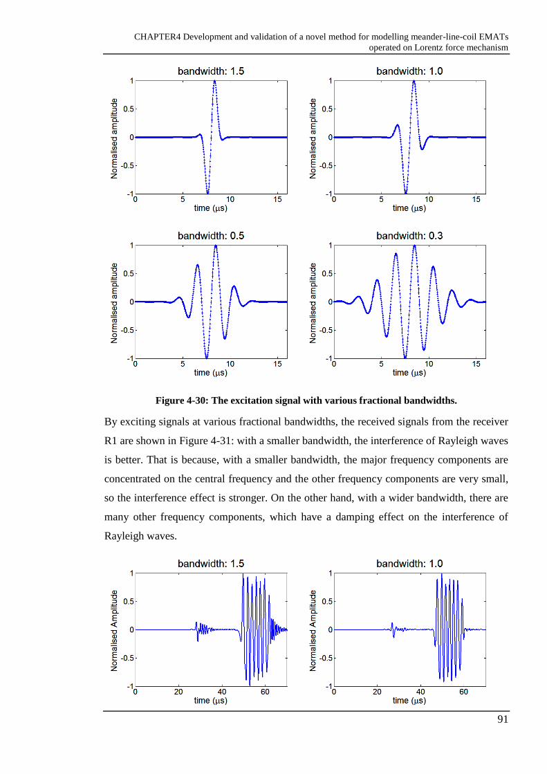
CHAPTER4 Development and validation of a novel method for modelling meander-line-coil EMATs
operated on Lorentz force mechanism
91
Figure 4-30: The excitation signal with various fractional bandwidths.
By exciting signals at various fractional bandwidths, the received signals from the receiver
R1 are shown in Figure 4-31: with a smaller bandwidth, the interference of Rayleigh waves
is better. That is because, with a smaller bandwidth, the major frequency components are
concentrated on the central frequency and the other frequency components are very small,
so the interference effect is stronger. On the other hand, with a wider bandwidth, there are
many other frequency components, which have a damping effect on the interference of
Rayleigh waves.
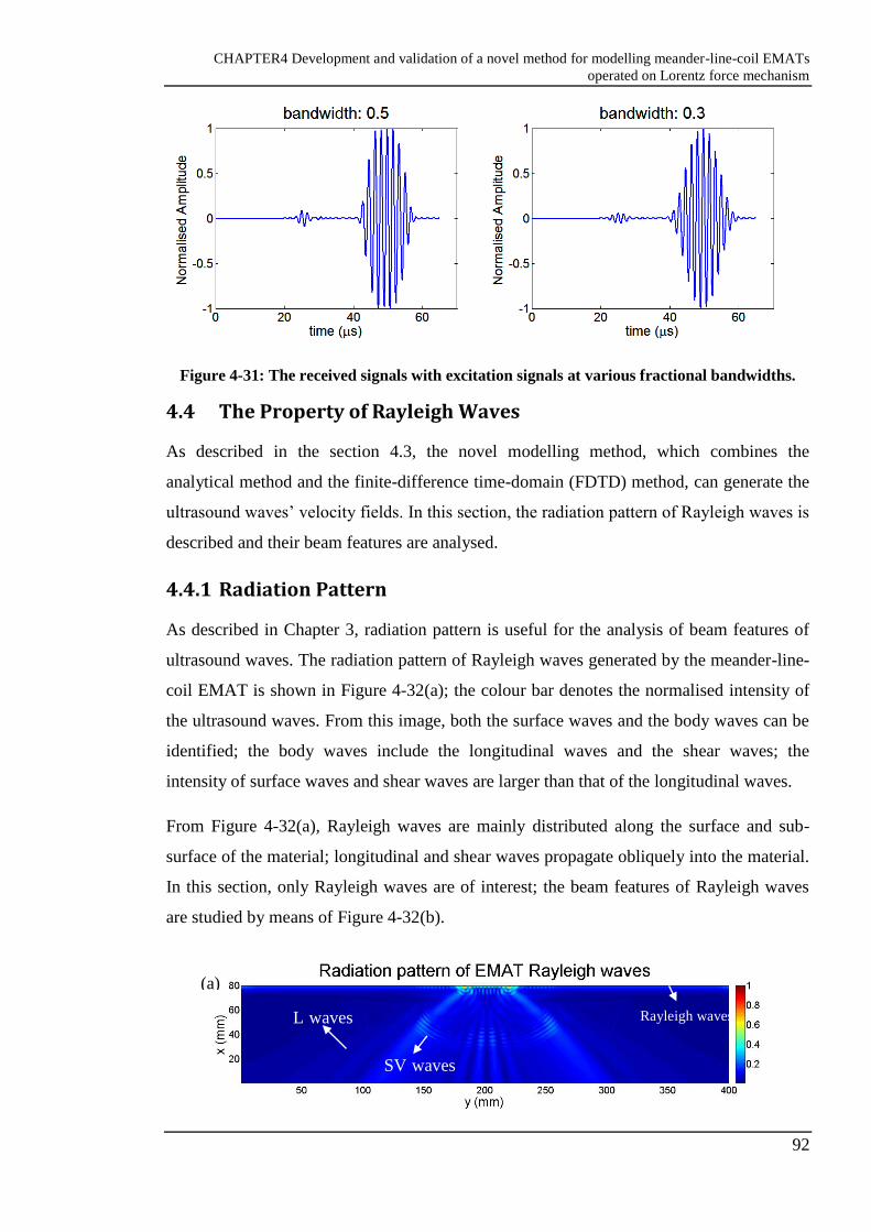
CHAPTER4 Development and validation of a novel method for modelling meander-line-coil EMATs
operated on Lorentz force mechanism
92
Figure 4-31: The received signals with excitation signals at various fractional bandwidths.
4.4 The Property of Rayleigh Waves
As described in the section 4.3, the novel modelling method, which combines the
analytical method and the finite-difference time-domain (FDTD) method, can generate the
ultrasound waves’ velocity fields. In this section, the radiation pattern of Rayleigh waves is
described and their beam features are analysed.
4.4.1 Radiation Pattern
As described in Chapter 3, radiation pattern is useful for the analysis of beam features of
ultrasound waves. The radiation pattern of Rayleigh waves generated by the meander-line-
coil EMAT is shown in Figure 4-32(a); the colour bar denotes the normalised intensity of
the ultrasound waves. From this image, both the surface waves and the body waves can be
identified; the body waves include the longitudinal waves and the shear waves; the
intensity of surface waves and shear waves are larger than that of the longitudinal waves.
From Figure 4-32(a), Rayleigh waves are mainly distributed along the surface and sub-
surface of the material; longitudinal and shear waves propagate obliquely into the material.
In this section, only Rayleigh waves are of interest; the beam features of Rayleigh waves
are studied by means of Figure 4-32(b).
L waves
wavesw
aves SV waves
waves
Rayleigh waves
(a)

CHAPTER4 Development and validation of a novel method for modelling meander-line-coil EMATs
operated on Lorentz force mechanism
93
Figure 4-32: (a), the radiation pattern of the EMAT-Rayleigh waves; (b), the radiation
pattern used for the analysis of beam features.
There are two beam features, beam directivity and field distribution along the steering
angle, to be analysed. In Figure 4-32(b), r denotes the radial distance from the centre of the
sensor, 𝜃 denotes the steering angle; define the angle parallel to the surface is 00; in order
to minimise the effects of the longitudinal waves and shear waves, keep the radial distance
r to 140 mm and the steering angle 𝜃 from 00 to 200.
4.4.2 Beam Features
The beam directivity calculated is shown in Figure 4-33, which shows the relationship
between the steering angle and the magnitude of the velocity fields; the magnitude of the
velocity fields is normalised. From this figure, Rayleigh waves are mainly concentrated at
angles from 00 to 2.50, and the peak occurs at the angle 00; when the steering angle is
beyond the range from 00 to 2.50, the magnitude of Rayleigh waves decays to a level lower
than 20 percent of the peak value; this further verifies the Rayleigh waves are concentrated
on the surface and the subsurface of the material.
Because the radial distance r used is 140 mm and the steering angle range of Rayleigh
waves is from 00 to 2.50, Rayleigh waves are concentrated on a depth calculated by
Equation 4-9.
Equation 4-9
𝑑 = 𝑡𝑎𝑛(𝜃) ∗ 𝑟
The depth d calculated is 6.1 mm, and the wavelength of the Rayleigh waves used in this
work is 6.066 mm, which indicates that the Rayleigh waves are mainly distributed within
one wavelength of the Rayleigh waves. In addition, when choose another value of the
radial distance r, the angle 𝜃 changes correspondingly, but the depth d of the Rayleigh
waves’ distribution is a constant.
𝜃 𝑟 (b)
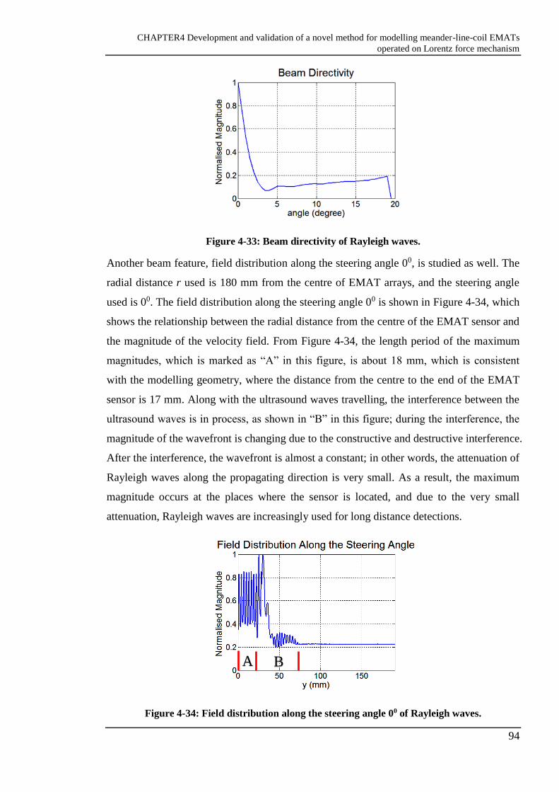
CHAPTER4 Development and validation of a novel method for modelling meander-line-coil EMATs
operated on Lorentz force mechanism
94
Figure 4-33: Beam directivity of Rayleigh waves.
Another beam feature, field distribution along the steering angle 00, is studied as well. The
radial distance r used is 180 mm from the centre of EMAT arrays, and the steering angle
used is 00. The field distribution along the steering angle 00 is shown in Figure 4-34, which
shows the relationship between the radial distance from the centre of the EMAT sensor and
the magnitude of the velocity field. From Figure 4-34, the length period of the maximum
magnitudes, which is marked as “A” in this figure, is about 18 mm, which is consistent
with the modelling geometry, where the distance from the centre to the end of the EMAT
sensor is 17 mm. Along with the ultrasound waves travelling, the interference between the
ultrasound waves is in process, as shown in “B” in this figure; during the interference, the
magnitude of the wavefront is changing due to the constructive and destructive interference.
After the interference, the wavefront is almost a constant; in other words, the attenuation of
Rayleigh waves along the propagating direction is very small. As a result, the maximum
magnitude occurs at the places where the sensor is located, and due to the very small
attenuation, Rayleigh waves are increasingly used for long distance detections.
Figure 4-34: Field distribution along the steering angle 00 of Rayleigh waves.
A B

CHAPTER4 Development and validation of a novel method for modelling meander-line-coil EMATs
operated on Lorentz force mechanism
95
4.5 EMAT-receiving Mechanism
As described in section 4.3, the velocity fields can be obtained by combining the EMAT-
EM modelling and the EMAT-US modelling. In the presence of a static magnetic field,
such velocity fields can induce the time varying magnetic field, which can be picked up by
the receiving coil.
In this part, the induced voltage calculation is introduced based on the solution proposed
by [21]. The model used for studying the receiving process is shown in Figure 4-35, where
the modelling geometry is divided into four zones. Zone 0 is the region where the
permanent magnet located at; zone 1 contains the meander-line-coil and the surrounded air;
zone 2 and zone 3 are the material with the same property. The permanent magnet and the
meander-line-coil used in the receiving transducer is exactly the same as those used in the
transmitting transducer; the permanent magnet is accurately placed on the top of the coil.
Figure 4-35: The model used for calculating the induced voltage in the receiving coil.
The ultrasonic waves, in the presence of a static magnetic field, induce the eddy current in
the material as shown in Equation 4-10; ved is the velocity field at the depth of xed; Eed and
Jed are the induced electric field and the induced current at the depth of xed respectively. B
is the static magnetic field, σ is the conductivity of the material,
Equation 4-10
{𝑬𝑒𝑑 = 𝒗𝒆𝒅 × 𝑩𝑱𝑒𝑑 = 𝜎 ∙ 𝑬𝑒𝑑
Due to the induced current 𝑱𝒆𝒅 at the depth of xed, the vector potential is generated into the
permanent magnet (zone 1), the air area with the meander-line-coil (zone 2), and the

CHAPTER4 Development and validation of a novel method for modelling meander-line-coil EMATs
operated on Lorentz force mechanism
96
conductor (zone 3 and zone 4). Based on Maxwell’s Equations, the vector potentials in
different zones are described in Equation 4-11, where Ai, σi and µi are the vector potential,
the conductivity and the permeability respectively; the subscript i corresponds to different
zones. ω is the angular frequency; j is √−1.
Equation 4-11
{
𝛻2𝑨0 = 𝑗𝜔𝜎0𝜇0𝑨0 𝛻2𝑨1 = −𝜔
2𝜀1𝜇1𝑨1𝛻2𝑨2 = 𝑗𝜔𝜎2𝜇2𝑨2𝛻2𝑨3 = 𝑗𝜔𝜎3𝜇3𝑨3
The total vector potential in zone 1 generated by the entire eddy current in the material can
be obtained by integrating over the depth of zone 2, 𝑥𝑒𝑑, (Equation 4-12), where 𝑨 denotes
the entirely induced vector potential in the region of air (zone 1). The entire vector
potential in zone 1 produces the induced voltage which can be picked up by the receiving
EMAT (Equation 4-13). Er and Vr are the induced electric field and the induced voltage
respectively; 𝑁and ℓ are the turn number and the length of the receiving coil respectively.
Equation 4-12
𝑨 = ∫ 𝑨1𝑑 (𝑥𝑒𝑑)0
−∞
Equation 4-13
{𝑬𝑟 = −𝜕𝑨
𝜕𝑡𝑽𝑟 = 𝑁ℓ𝑬𝑟
4.6 Experimental Validations
4.6.1 Experiments Set-up
In this section, experiments were conducted to validate the proposed modelling methods as
described in section 4.3. A high power tone burst pulser / receiver, RITEC RPR4000, was
used. RITEC RPR4000 is capable of pulsing up to 8 kW, hence it is desirable for
inefficient transducers, such as electromagnetic acoustic transducers (EMATs); the
standard operational frequency range of RITEC RPR4000 is from 250 kHz to 5 MHz. The
gain of the receiver is from 20 dB to 100 dB; the filter has a passband from 50 kHz to 20
MHz; in this work, the gain of the receiver used was 80 dB, and the passband filter used

CHAPTER4 Development and validation of a novel method for modelling meander-line-coil EMATs
operated on Lorentz force mechanism
97
was from 200 kHz to 2.5 MHz, which means only the signal at the frequency range from
200 kHz to 2.5 MHz can be received. RITEC RPR4000 can be connected to an external
computer via the serial interface RS-232.
The schematic diagram of the experimental system is shown in Figure 4-36; the high
power tone burst pulser and receiver, RITEC RPR4000, was used to excite and receive
EMAT signals; the impedance matching box was used to match the impedance between
the power amplifier and the coil to maximize power transfer; the transmitter and receiver
consist of the permanent magnet and the meander coil as described in the part of EMAT
simulation; oscilloscope was used to display and record signals. Data can be sent to the
external computer to process either by RITEM RPR4000 or by the oscilloscope.
Figure 4-36: The schematic diagram of the experimental system.
Figure 4-37 shows the set-up of the experimental system; the stainless-steel plate, the
meander-line-coil and the permanent magnet used had the same dimension and shapes as
those clarified in section 4.1.1. The transmitter and the receiver were located on the top of
the stainless steel plate with a centre-to-centre distance of 150 mm. The effect of the
fractional bandwidth has been described in section 4.3.4, which states a small factional
bandwidth, 0.3, for the central frequency 500 kHz is sufficiently reliable for Rayleigh
waves’ interference. For the experiments, the excitation voltage used is a Gaussian-
modulated sinusoidal wave with a peak voltage of 140 V, and the fractional width used is
0.18, which can provide a good signal resolution. The sampling frequency is 100 MHz
from the oscilloscope.

CHAPTER4 Development and validation of a novel method for modelling meander-line-coil EMATs
operated on Lorentz force mechanism
98
Figure 4-37: Set-up of the experimental system.
4.6.2 Received Signals from Experiments
Because the EMAT transmitter is operated at 500 kHz, the received signal is mainly
concentrated on 500 kHz as well. The output of the fast Fourier transform of the originally
received signal from experiments is shown in Figure 4-38(a); as expected, the major
frequency component is 500 kHz. However, there were some other frequency components,
such as 1 MHz and 1.5 MHz, which are not desirable and should be cut-off. By processing
signals, a band-pass filter is employed to allow the frequency from 480 kHz to 520 kHz to
pass. The filtered signal is shown in Figure 4-38(b); the non-desirable signal are cut-off,
and the signal are mainly concentrated on the operational frequency, 500 kHz.
Figure 4-38: The frequency domain of the experimentally received signals.
Oscilloscope RPR-4000
Receiver
Transmitter
(a) (b)
Impedance matching box
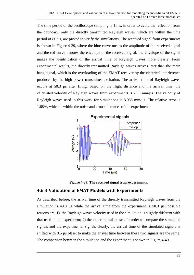
CHAPTER4 Development and validation of a novel method for modelling meander-line-coil EMATs
operated on Lorentz force mechanism
99
The time period of the oscilloscope sampling is 1 ms; in order to avoid the reflection from
the boundary, only the directly transmitted Rayleigh waves, which are within the time
period of 80 µs, are picked to verify the simulations. The received signal from experiments
is shown in Figure 4-39, where the blue curve means the amplitude of the received signal
and the red curve denotes the envelope of the received signal; the envelope of the signal
makes the identification of the arrival time of Rayleigh waves more clearly. From
experimental results, the directly transmitted Rayleigh waves arrives later than the main
bang signal, which is the overloading of the EMAT receiver by the electrical interference
produced by the high power transmitter excitation. The arrival time of Rayleigh waves
occurs at 50.3 µs after firing; based on the flight distance and the arrival time, the
calculated velocity of Rayleigh waves from experiments is 2.98 mm/µs. The velocity of
Rayleigh waves used in this work for simulations is 3.033 mm/µs. The relative error is
1.68%, which is within the noise and error tolerances of the experiments.
Figure 4-39: The received signal from experiments.
4.6.3 Validation of EMAT Models with Experiments
As described before, the arrival time of the directly transmitted Rayleigh waves from the
simulation is 49.8 µs while the arrival time from the experiment is 50.3 µs; possible
reasons are, 1), the Rayleigh waves velocity used in the simulation is slightly different with
that used in the experiment; 2) the experimental noises. In order to compare the simulated
signals and the experimental signals clearly, the arrival time of the simulated signals is
shifted with 0.5 µs offset to make the arrival time between these two signals are the same.
The comparison between the simulation and the experiment is shown in Figure 4-40.

CHAPTER4 Development and validation of a novel method for modelling meander-line-coil EMATs
operated on Lorentz force mechanism
100
By multiplying a scaling factor, simulation signals have the same peak value with the
experimental signals as shown in Figure 4-40, where the simulation shows a good
agreement with the experiment. In this section, root-mean-square error (RMSE) and the
correlation coefficient are employed to describe the difference and the linear correlation
between the simulated and experimental models. The time period of the received Rayleigh
waves is from 30 µs to 70 µs as shown in Figure 4-40; the root-mean-square error (RMSE)
within this time period calculated is 0.0834, which shows a very small difference between
the simulated model and the experiment model. The correlation coefficient calculated is
0.9927, which shows the simulated model and the experimental model are highly
correlated.
However, at the beginning and the end of Rayleigh waves (as shown in the “Note Area” in
Figure 4-40), there is a slight difference between the simulation and the experiment. More
specifically, the phases of the signals between the simulation and the experiment are not
consistent in the “Note Area”. Possible reasons are: 1), in this work, the simulated model is
a simplified model with only surface sources; 2), the numerical nature of FDTD: numerical
approximations are inevitable; 3), the inevitable noises of the experiment.
Figure 4-40: The comparison between the simulation and the experiment.
Changing the centre-to-centre distance between the transmitter and the receiver from 140
mm to 190 mm with a step of 10 mm, the maximum amplitude of the directly transmitted
Rayleigh waves from the simulation and the experiment are shown in Figure 4-41, which
show a good agreement. From Figure 4-41, the induced voltage decreases with the distance
Note Area

CHAPTER4 Development and validation of a novel method for modelling meander-line-coil EMATs
operated on Lorentz force mechanism
101
between the transmitter and the receiver increasing; that is due to the attenuation of
Rayleigh waves. However, the attenuation is very small; from the simulation, the
attenuation is 0.0034% with a travelling distance of 5 cm; from the experiment, the
attenuation is 0.0039% with a travelling distance of 5 cm.
Figure 4-41: The maximum amplitude of the induced voltage with various distances between
the transmitter and the receiver.
It should be noted that, for the EMATs modelling as described in section 4.3, the dynamic
magnetic field was neglected due to the small excitation AC current used in this work; the
excitation voltage used was a Gaussian-modulated sinusoidal wave with a peak voltage of
140 V and the impedance of the meander-line-coil at 500 kHz was 27.65 Ω, hence the
excitation current approximately equals to 5.06 A. Experiments with only the meander-
line-coil to generate Rayleigh waves were carried out to study the effect of the dynamic
magnetic field; the transmitter used was a meander-line-coil without the permanent magnet;
the other set-up were the same as those clarified in section 4.6.1. The received signals with
only the meander-line-coil as the transmitter is shown in Figure 4-42; only the main bang
signal can be captured by the receiving EMAT, and therefore the effect of the dynamic
magnetic field can be neglected due to the small excitation current used in this work. The
effect of the dynamic magnetic field generated by the meander-line-coil must be
considered when the excitation current is large as it is one of the mechanisms to generate
ultrasound waves; [39] suggested, when the excitation exceeds 528.9 A, the dynamic
magnetic field plays a more significant role than the static magnetic field, which is
generated by the permanent magnet.
0.995
0.996
0.997
0.998
0.999
1
14 15 16 17 18 19
No
rma
lise
d V
olt
ag
e
Distance between the transmitter and the receiver (cm)
Induced Voltage
Experiment Simulation

CHAPTER4 Development and validation of a novel method for modelling meander-line-coil EMATs
operated on Lorentz force mechanism
102
Figure 4-42: The received signals with a meander-line-coil as the transmitter.
4.7 EMAT Scattering Phenomena
Previously, the Rayleigh waves’ property generated by meander-line-coil EMATs have
been analysed with a novel modelling method, which combines the analytical method and
the finite-difference time-domain (FDTD) method; this method has been verified with
experiments as described in section 4.6.
Rayleigh waves propagate along the surface and the subsurface of the test piece; due to the
nature of a low attenuation and a long distance propagation, Rayleigh waves are
increasingly used in applications of surface and sub-surface cracks detections. In this
section, the scattering behaviour of Rayleigh wave is studied by means of the proposed
modelling method and experiments.
4.7.1 Modelling of Rayleigh Waves’ Scattering
4.7.1.1 Scattering Models and Wave Propagations
In section 4.3.2, in order to identify the body waves clearly, a thicken model with a depth
of 80 mm is used. Because only Rayleigh waves are of interest in this section, the thickness
of the stainless steel plate is set to 25 mm. The modelling geometry is shown in Figure
4-43; where the sources are the alternating Lorentz force densities from the EM simulation
as described in section 4.2.4. Free surface is applied on the top of the modelling geometry;
perfectly-matched layers (PML) are used to absorb reflections from left, right and bottom
boundaries of the material. A crack with a width of 0.5 mm and a depth of 2 mm is placed
on x=25 mm and y=500 mm; two virtual receivers, R1 and R2, are placed on x=24 mm and
y=400 mm, and x=24 mm and y=550 mm, to inspect Rayleigh waves. The spatial step and

CHAPTER4 Development and validation of a novel method for modelling meander-line-coil EMATs
operated on Lorentz force mechanism
103
the time step, the operational frequency, the spacing between the adjacent sources, and the
Rayleigh waves’ velocity used are the same as those used in section 4.3.
Figure 4-43: The geometry of Rayleigh waves’ scattering simulation.
The Rayleigh waves’ propagation is shown in Figure 4-44, which visualizes the scattering
behaviour of the EMAT-Rayleigh waves. At 10 µs after firing, both the body waves and
the Rayleigh waves are generated into the material (Figure 4-44(a)). Due to the PML
boundary applied to the bottom of the material, obliquely propagated body waves are
absorbed; as shown in Figure 4-44(b) and Figure 4-44(c), only Rayleigh waves exist in
these images. The directly transmitted Rayleigh waves, abbreviated for “DRW”, are
received by the receiver R1. At 67 µs after firing, the directly transmitted Rayleigh waves
encounter the crack, and are reflected and scattered by the crack (Figure 4-44(d)). The
reflected Rayleigh waves are abbreviated for “RRW” and the scattered Rayleigh waves are
abbreviated for “SRW” as shown in Figure 4-44(e). The scattered Rayleigh waves (SRW)
are received by the receiver R2 (Figure 4-44(f)), and the reflected Rayleigh waves (RRW)
are received by the receiver R1 (Figure 4-44(g)).
(b) DRW
(a)

CHAPTER4 Development and validation of a novel method for modelling meander-line-coil EMATs
operated on Lorentz force mechanism
104
Figure 4-44: Scattering behaviours of Rayleigh waves.
4.7.1.2 Received Signals from Simulations
The induced voltage picked up by the receiver R1 is shown in Figure 4-45, where the blue
curve shows the normalised amplitude of the induced voltage, and the red curve shows the
normalised envelope of the received signal based on Hilbert transform, resulting in
identification of the arrival signals more clearly [7].
From Figure 4-45, two signals are received by the receiver R1; the firstly arriving signal is
the DRW followed by the RRW. The centre-to-centre distance between the transmitter and
the receiver is 100 mm, and the Rayleigh waves’ velocity used in this work is 3.033 mm/µs,
so the theoretically arrival time of the DRW is 32.97 µs. The numerally arrival time of the
DRW, as shown in Figure 4-45, is 32.94 µs, which shows a good agreement with the
theoretically arrival time 32.97 µs.
The travelling distance of the RRW is 300 mm, and the Rayleigh waves’ velocity used in
this work is 3.033 mm/µs, hence the theoretically arrival time of the RRW is 98.91 µs,
which is very close to the numerically arrival time of the RRW 100.3 µs.
RRW SRW
SRW
RRW
DRW (c)
(d)
(e)
(f)
(g)

CHAPTER4 Development and validation of a novel method for modelling meander-line-coil EMATs
operated on Lorentz force mechanism
105
Figure 4-45: Received signals from R1.
The received signals of R2 are slightly different from those of R1 (Figure 4-46). There is
no DRW, because the DRW are scattered by the crack; only the SRW are picked up by the
receiver R2; the numerically arrival time of the SRW, as shown in Figure 4-46, is 82.95 µs.
The centre-to-centre distance between the transmitter and the receiver is 250 mm, and the
Rayleigh waves’ velocity used in this work is 3.033 mm/µs, so the theoretically arrival
time of the SRW is 82.43 µs. The relative error between the theoretically arrival time and
the numerically arrival time is 0.63%, which is very small to show a good agreement.
Figure 4-46: Received signals from R2.
The comparison between the received signals from R1 and R2 is shown in Figure 4-47,
where the blue curve shows the received signal from the receiver R1 and the red curve
shows the received signal from the receiver R2; the amplitude of the received signal is
normalised. From this image, the arrival time of the SRW is smaller than that of the RRW;
0 50 100-1
-0.5
0
0.5
1
Simulated Signals: R1
time (s)
Norm
alis
ed V
oltage
Amplitude
Envelope
0 50 100-1
-0.5
0
0.5
1
Simulated Signals: R2
time (s)
Norm
alis
ed V
oltage
Amplitude
Envelope

CHAPTER4 Development and validation of a novel method for modelling meander-line-coil EMATs
operated on Lorentz force mechanism
106
that is because the travelling distance of the SRW is smaller than that of the RRW. In
addition, the amplitude of the SRW is smaller than that of the RRW; this indicates the
DRW are mainly reflected; in other words, only a small portion of the DRW propagates
forward with the specific crack used in this work.
Figure 4-47: The comparison of the received signals from the receivers R1 and R2.
4.7.2 Experiments and Validations
4.7.2.1 Received Signals from Experiments
In this section, experiments were carried out to validate the scattering simulation;
experimental system has been detailed in section 4.6.1. The transmitter, the receiver and
the material used in the experiment were the same as those used in the scattering
simulation. The excitation signal, the operational frequency and the sampling frequency
were exactly the same as those used section 4.6.1.
In the scattering modelling, two receivers, R1 and R2, were employed. For experiments,
only the received signal from the receiver R1 was used to validate the proposed modelling
method. The experimentally received signal from the receiver R1 is shown in Figure 4-48,
where the blue curve and the red curve denote the amplitude and the envelope of the
induced voltage in the pick-up coil respectively. Three signals, the main bang signal, the
DRW and the RRW were picked up by the receiving coil.
As expected, the DRW arrives earlier with an arrival time around 33 µs and the RRW
arrives latter with an arrival time around 100 µs. The theoretically arrival time of these two
RRW SRW
DRW

CHAPTER4 Development and validation of a novel method for modelling meander-line-coil EMATs
operated on Lorentz force mechanism
107
signals are 32.97 µs and 98.91 µs; there is a slight difference between the experimentally
arrival time and the theoretically arrival time due to the experimental noise.
Figure 4-48: The experimentally received signal from the receiver R1.
4.7.2.2 Validations
The comparison between the simulated signal and the experimental signal is shown in
Figure 4-49, where the blue curve and the red curve denote the received signal from
simulations and the received signal from experiments respectively. Due to the slight
difference of the arrival time between the experiment and the simulation, an arrival time
shift is applied to make these two signals synchronized. In addition, a scaling factor is used
to keep the amplitude of the DRW between the simulation and the experiment to a same
value.
From Figure 4-49, the simulated signal and the experimental signal shows a good
agreement. In order to compare these two signals quantitatively, the root-mean-square
error (RMSE) and the correlation coefficient are employed. In addition, in order to
eliminate the effect of the main bang signal, only the signal within the time period from 12
µs to 145 µs is picked. The RMSE within this time period calculated is 0.1159, which
shown a small difference between the simulated model and the experimental model. The
correlation coefficient calculated is 0.9241, which means the simulated model and the
experimental model are highly correlated.
0 50 100-3
-2
-1
0
1
2
3
Experimental Signals
time (s)
Voltage (
V)
Amplitude
Envelope

CHAPTER4 Development and validation of a novel method for modelling meander-line-coil EMATs
operated on Lorentz force mechanism
108
Figure 4-49: The amplitude comparison between the simulation and the experiment.
In addition, the envelope comparison between these two signals are studied as well, as
shown in Figure 4-50. The difference between these two signals are more clearly by
comparing the envelope; the simulated signal is slightly narrower than the experimentally
received signal, no matter in the DRW or in the RRW. For the envelope comparison, the
RMSE calculated is 0.0784 and the correlation coefficient calculated is 0.9841, which
further verifies the small difference between the simulated model and the experimental
model.
Figure 4-50: The envelope comparison between the simulation and the experiment.
4.8 Modelling of Unidirectional Rayleigh Waves EMATs
Typically, the Rayleigh waves generated by the meander-line-coil travel are symmetrically
in two directions, as shown in Figure 4-27. This type of EMAT is named the bidirectional
Rayleigh waves (BRW) EMAT; the BRW EMAT has a non-desirable feature that the
0 50 1000
0.5
1
1.5
2
2.5
Comparison: Envelope
Time (s)
Voltage (
V)
Simulations
Experiments

CHAPTER4 Development and validation of a novel method for modelling meander-line-coil EMATs
operated on Lorentz force mechanism
109
crack detection resolution is low due to the two-directionally symmetrically propagating
Rayleigh waves. In order to improve the crack detection resolution, there is a demand for
the EMAT to generate unidirectional Rayleigh waves.
In 2013, [23] reported an EMAT which is capable of generating unidirectional Rayleigh
waves with two identical meander-line-coils; this type of EMAT is named the
unidirectional Rayleigh waves (URW) EMAT. The configuration of the URW EMAT is
shown in Figure 4-51; the URW EMAT consists of a permanent magnet, a test piece and
two identical meander-line-coils. The interaction between the eddy current and the static
magnetic field generates the Lorentz force density, which in turn produces ultrasound
waves.
Figure 4-51: The configuration of the URW EMAT. From [23].
This URW EMAT has been detailed in [23]; here a brief description about the wave
superposition for the URW EMAT is presented. Define these two identical meander-line-
coils as coil A and coil B, as described in Figure 4-51; both coil A and coil B have a
centre-to-centre distance of adjacent wires equalling to a half of Rayleigh waves’
wavelength λ/2. The distance between coil A and coil B is a quarter of Rayleigh waves’
wavelength λ/4; the excitation signal for coil A and coil B has the same amplitude but a
phase difference of 900. The wave superposition is shown in Figure 4-52; the source 1 is
generated by the coil A while the source 2 is generated by the coil B; source 1 and source 2
have a distance of a quarter of Rayleigh waves’ wavelength λ/4. Based on the wave
interference, the synthetic wave is generated, with the amplitude strengthen in one
direction while weaken in the other direction [80].

CHAPTER4 Development and validation of a novel method for modelling meander-line-coil EMATs
operated on Lorentz force mechanism
110
Figure 4-52: The wave superposition between the source 1 and the source 2. From [80].
In this section, the proposed modelling method is used to study the URW EMAT
properties. The EM simulation is performed with the analytical method and the US
simulation is accomplished by the finite-difference time-domain (FDTD) method as
described in section 4.3. The operational frequency, the material, the magnet and the
related parameters are the same as those used in section 4.1.1. The excitation signals for
Coil A and Coil B are shown in Figure 4-53; the operational frequency is 500 kHz and the
phased difference between Coil A and Coil B is 900; that means the central pulse time
between Coil A and Coil B has a shift of 0.5 µs.
Figure 4-53: The excitation signal for the coil A and the coil B.
The wave propagation of Rayleigh waves generated by the URW EMAT is shown in
Figure 4-54; the image shows the distribution of the magnitude of Rayleigh waves. From

CHAPTER4 Development and validation of a novel method for modelling meander-line-coil EMATs
operated on Lorentz force mechanism
111
Figure 4-54(a), not only the Rayleigh waves, but also the shear waves are travelling in one
specific direction. From Figure 4-54(b), Rayleigh waves are more clear; the strengthen
Rayleigh waves are shown in the red ellipse and the weaken Rayleigh waves are shown in
the yellow ellipse. It is clearly that the strengthen Rayleigh waves have a larger intensity
than the weaken ones.
Figure 4-54: The wave propagation of Rayleigh waves generated by the URW-EMAT.
In order to quantitatively analyse the strengthen Rayleigh waves, two receivers are located
on the left and the right of the transmitter with a centre-to-centre distance of 145 mm from
the transmitter; specifically, the transmitter is located on x=79mm, y=200mm, and the
receiver on the left (termed as RL) is located on x=79mm, y=55 mm, and the receiver on
the right (termed as RR) is located on x=79mm, y=345 mm. The received signals from the
receivers RL and RR are shown in Figure 4-55; where the blue curve is the amplitude of
the weakened Rayleigh waves and the red curve is the amplitude of the strengthen
Rayleigh waves. The maximum amplitude of the strengthen Rayleigh waves is 8.5 times
as larger as that of the weakened Rayleigh waves.
(a)
(b)

CHAPTER4 Development and validation of a novel method for modelling meander-line-coil EMATs
operated on Lorentz force mechanism
112
Figure 4-55: The received signal from the URW-EMAT.
Figure 4-56 illustrates the received signal from the BRW EMAT, which is capable of
generating bidirectional Rayleigh waves. Two receivers, RL and RR, are located at a
distance of 145 mm from the transmitter. From this figure, the received signal from the
receiver RL and that from the receiver RR are almost the same; the ratio between the
maximum amplitude of the received signals from the receiver RL and that from the
receiver RR is 1.0002.
Figure 4-56: The received signal from the BRW-EMAT.
The comparison between the URW EMAT and the BRW EMAT is shown in Figure 4-57,
where Figure 4-57(a) shows the received signal from the receiver RL and Figure 4-57(b)
shows the received signal from the receiver RR. It can be identified that the Rayleigh
waves travelling to the left are suppressed with the URW EMAT; and Rayleigh waves
travelling to the right are amplified with the URW EMAT. The suppressed ratio is 0.2336

CHAPTER4 Development and validation of a novel method for modelling meander-line-coil EMATs
operated on Lorentz force mechanism
113
and the amplified ratio is 1.9849. All of these results are consistent with the results from
[23].
Figure 4-57: The comparison between the URW and the BRW.
4.9 Conclusions
In this chapter, a novel modelling method combining the analytical method and the finite-
difference time-domain (FDTD) method for simulating the meander-line-coil EMAT was
proposed by the author; the analytical method is used for the EM simulation and the FDTD
method is used for the US simulation.
The analytical method was adapted from the classic Dodd and Deeds solution for the eddy
current phenomena, and was verified by the finite element method (FEM). For the US
simulation, the FDTD method was used to model the ultrasound waves’ propagation,
analyse the radiation pattern and study the beam features of the generated Rayleigh waves.
The scattering behaviour of Rayleigh waves was modelled with the proposed modelling
method as well.
In addition, the novel modelling method is capable of modelling unidirectional Rayleigh
waves EMATs as well. Quantitatively analysis of the received signal was carried out; the
results showed that the unidirectional Rayleigh waves EMAT is able to strengthen the
Rayleigh waves in one direction and weaken that in the other direction.
Experiments were carried out to validate the novel modelling method; a good agreement
was observed between the experimental model and the numerical model. The RMSE and
the correlation coefficient were employed to quantitatively analyse the model difference
level and the model related level.
(a) (b)

CHAPTER4 Development and validation of a novel method for modelling meander-line-coil EMATs
operated on Lorentz force mechanism
114
Overall, the novel modelling method proposed by the author is capable of modelling
various behaviours of Rayleigh waves, such as bidirectional Rayleigh waves, scattering
Rayleigh waves, and unidirectional Rayleigh waves.

CHAPTER5 Directivity analysis of the conventional meander-line-coil EMATs
115
Chapter 5 Directivity Analysis of Conventional Meander-
line-coil EMATs
5.1 Introduction
Because 3-D modelling has a high requirement on computing power and requires
significant running time, most of the previous works were 2-D simulation focusing on the
vertical plane (i.e. x-y plane) of the material. The orientation of the coordinate system is
shown in Figure 4-1, and all of the subsequent simulations are based on this coordinate
system. Two examples of the 2-D modelling methods for the x-y plane of the material have
been detailed in [10, 13], however, there has been little research on the beam directivity of
Rayleigh waves on the surface plane (i.e. y-z plane) of the material.
This chapter presents a wholly analytical modelling method to study the beam directivity
of Rayleigh waves on the surface of the material. This wholly analytical method, which
involves the coupling of two models: an analytical EM model and an analytical US model,
has been developed to build EMAT models and analyse the beam directivity of Rayleigh
waves. Lorentz forces are calculated using the EM analytical method, which is adapted
from the classic Dodd and Deeds solution, as described in section 4.2. The calculated
Lorentz force density are imported to the analytical US model as driving point sources,
which produce the Rayleigh waves within a layered medium. Because the analytical EM
model is the same as the one used in section 4.2, this chapter only introduces the analytical
US model. The effect of the length of the meander-line-coil on the beam directivity of
Rayleigh waves is analysed quantitatively and validated experimentally.
5.2 The Analytical Solution to the Radiation Pattern of Rayleigh
Waves on the Surface of the Material
N. A. Haskell proposed the analytical solution to the Rayleigh waves’ radiation pattern due
to point sources in a homogenous medium and in a multi-layered medium, in 1963 and
1964 respectively [81, 82]. Elastic waves radiate in an unbounded medium expressed in
Cartesian coordinates was given by Love [83]. However, Sezawa’s cylindrical wave
functions are the most convenient ways to impose the free surface boundary conditions;
hence, the transformation between these two representations are necessary; the free surface
conditions are imposed by vanishing the stress components at the free surface. Rayleigh

CHAPTER5 Directivity analysis of the conventional meander-line-coil EMATs
116
waves’ components are separated out by calculating the residue at the Rayleigh pole [81,
82].
The articles, [81, 82], were published in the field of seismology, and some terminology in
the field of seismology, such as strike-slip faults and dip-slip faults, were used in these
articles [81, 82]. In this work, the driving source is the tangentially polarized Lorentz force,
which corresponds to the strike-slip fault; after some manipulations, the final solution to
the displacement of Rayleigh waves due to the surface point source is,
Equation 5-1
𝒖𝒓 = 𝐴(ĸ, 𝑟)𝑒−𝜋𝑖
42ĸ(𝛾−1)
𝑣𝛽∙ 𝑭 ∙ (
𝛾+1
𝛾− 1)
Equation 5-2
𝒖𝒙 =𝑖𝛾𝑣𝛼𝒖𝒓
ĸ(𝛾−1)
where
Equation 5-3
𝐴(ĸ, 𝑟) =ĸ2𝛾𝑣𝛽
4𝜌(2𝛾2𝑣𝛼𝑣𝛽
ĸ3)
√2
𝜋ĸ𝑟𝑒−𝑖ĸ𝑟
Equation 5-4
𝛾 = 𝑐𝑜𝑠 (𝜃)
Equation 5-5
𝑣𝛼 = {√ĸ2 − (𝜔/𝑐𝐿)2 ĸ > 𝜔/𝑐𝐿
𝑖√(𝜔/𝑐𝐿)2 − ĸ2 ĸ < 𝜔/𝑐𝐿
Equation 5-6
𝑣𝛽 = {√ĸ2 − (𝜔/𝑐𝑆)2 ĸ > 𝜔/𝑐𝑠
𝑖√(𝜔/𝑐𝑆)2 − ĸ2 ĸ < 𝜔/𝑐𝑠
Equation 5-7
ĸ =𝜔
𝑐𝑅
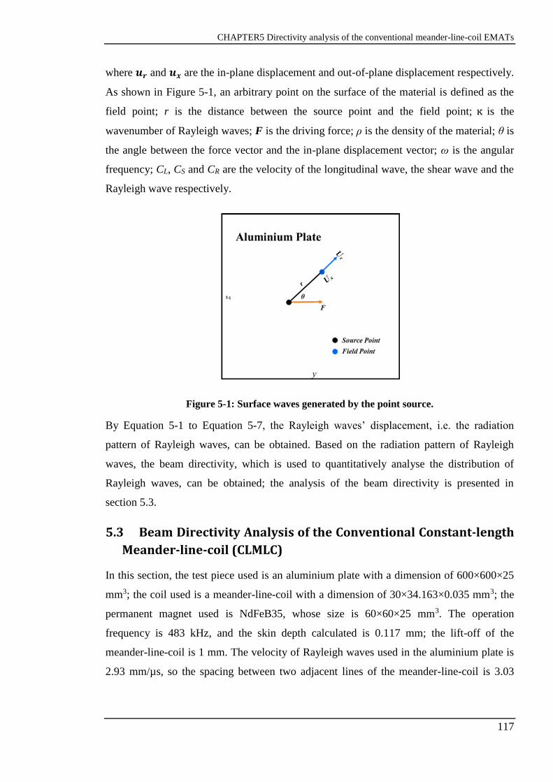
CHAPTER5 Directivity analysis of the conventional meander-line-coil EMATs
117
where 𝒖𝒓 and 𝒖𝒙 are the in-plane displacement and out-of-plane displacement respectively.
As shown in Figure 5-1, an arbitrary point on the surface of the material is defined as the
field point; r is the distance between the source point and the field point; ĸ is the
wavenumber of Rayleigh waves; F is the driving force; ρ is the density of the material; θ is
the angle between the force vector and the in-plane displacement vector; ω is the angular
frequency; CL, CS and CR are the velocity of the longitudinal wave, the shear wave and the
Rayleigh wave respectively.
Figure 5-1: Surface waves generated by the point source.
By Equation 5-1 to Equation 5-7, the Rayleigh waves’ displacement, i.e. the radiation
pattern of Rayleigh waves, can be obtained. Based on the radiation pattern of Rayleigh
waves, the beam directivity, which is used to quantitatively analyse the distribution of
Rayleigh waves, can be obtained; the analysis of the beam directivity is presented in
section 5.3.
5.3 Beam Directivity Analysis of the Conventional Constant-length
Meander-line-coil (CLMLC)
In this section, the test piece used is an aluminium plate with a dimension of 600×600×25
mm3; the coil used is a meander-line-coil with a dimension of 30×34.163×0.035 mm3; the
permanent magnet used is NdFeB35, whose size is 60×60×25 mm3. The operation
frequency is 483 kHz, and the skin depth calculated is 0.117 mm; the lift-off of the
meander-line-coil is 1 mm. The velocity of Rayleigh waves used in the aluminium plate is
2.93 mm/µs, so the spacing between two adjacent lines of the meander-line-coil is 3.03

CHAPTER5 Directivity analysis of the conventional meander-line-coil EMATs
118
mm, which equals to one half of the Rayleigh waves’ wavelength, to form the constructive
interference.
5.3.1 Wholly Analytical Models
For modelling Rayleigh waves on the surface of the material (i.e. the y-z plane of the
material), a wholly analytical method, which involves the coupling of an analytical EM
model and an analytical US model, is utilized. The analytical EM solution, which is
adapted from the classic Dodd and Deeds solution, has been introduced in section 4.2.
Lorentz force densities, which are generated from the analytical EM simulation, are
imported to the analytical US model, as shown in Figure 5-2.
There are 12 straight wires in the meander-line-coil used in this work; therefore, there are
12 negative and positive peaks in the curve of the Lorentz force density distribution. These
12 Lorentz force densities are added to the US model as driving forces to generate
Rayleigh waves. The displacement of Rayleigh waves due to a point source can be
calculated by Equation 5-1 to Equation 5-7; with multiple point sources, the displacement
of Rayleigh waves at an arbitrary field point is the sum of the displacement caused by each
point source.
Figure 5-2: The transformation between the analytical EM model and the analytical US
model.
Table 5-1 illustrates the detailed parameters used for the analytical US model. Field spatial
step means the distance between two adjacent field points on the surface of the Aluminium
plate; the dimension of the surface of the aluminium plate is 600×600 mm2 and the field
spatial step used is 1 mm, so there are totally 601×601 field points on the surface of the

CHAPTER5 Directivity analysis of the conventional meander-line-coil EMATs
119
Aluminium plate. Source spatial step for each wire means the distance between two
adjacent source points on each wire; the length of the wire is 30 mm and the source spatial
step used is 0.2 mm, so there are 151 source points on each wire. The reason we choose
dense source points is that lots of source points guarantee the wave interference’ integrity.
Table 5-1: Detailed parameters used for the analytical US model.
Description Symbol Value
Length of the Aluminum plate Y 600 mm
Width of the Aluminum plate Z 600 mm
Field spatial step ∆xf 1 mm
Length of the meander-line-coil L 30 mm
Source spatial step for each wire ∆xs 0.2 mm
Density of the Aluminum plate ρ 2700 kg/m3
Frequency f 483 kHz
Longitudinal waves’ velocity CL 6.375 mm/µs
Shear waves’ velocity Cs 3.14 mm/µs
Rayleigh waves’ velocity CR 2.93 mm/µs
The meander-line-coil is located on the centre of the aluminium plate, so the whole
EMAT-US model is symmetrical with y=300 mm; in order to reduce the modelling time,
only the left half of the geometry is modelled. Only the area, y from 0 to 250 mm, is
presented where the signals are significant. The calculated Rayleigh waves’ radiation
pattern is shown in Figure 5-3. From this image, it can be seen that the Rayleigh waves are
mainly concentrated along the y direction. The area with larger intensities is referred to as
the main lobe while the areas with smaller intensities are referred to as the side lobes, as
shown in Figure 5-3.

CHAPTER5 Directivity analysis of the conventional meander-line-coil EMATs
120
Figure 5-3: The Rayleigh waves’ radiation pattern on the surface of the aluminium plate.
The whole radiation pattern is shown in Figure 5-4; as mentioned previously, it is
symmetrical with y=300 mm. Beam directivity, which are used to quantitatively analyse
the Rayleigh waves’ distribution, can be obtained on the basis of the radiation pattern of
Rayleigh waves. As shown in the red arc in Figure 5-4, beam directivity is, at a specific
distance (“r” in Figure 5-4) from the centre of the EMAT sensor, the displacement
distribution of Rayleigh waves. In this work, r used is 250 mm; θ1 and θ2 used are -700 and
700 respectively.
Figure 5-4: The model used to study the beam directivity.
Main Lobe
Side Lobes

CHAPTER5 Directivity analysis of the conventional meander-line-coil EMATs
121
The calculated beam directivity is shown in Figure 5-5(a); this curve states the normalised
magnitude of the displacement versus angles. As observed, there is a main lobe containing
a larger displacement magnitude and some side lobes with smaller displacement
magnitudes. The main lobe is centred at 00, and the side lobes are roughly centred at -30.50,
-18.50, 18.50 and 30.50 respectively. The side lobes are usually the radiation in undesired
directions.
In order to quantitatively analyse the beam directivity, the half power beamwidth (HPBW)
and the sidelobe level (SLL) are utilized. The half power beamwidth (HPBW) is the angle
between the half-power (-3 dB) points of the main lobe; the half-power (-3 dB) points are
the points with a magnitude equalling to a half of the peak value of the main lobe, as
shown in Figure 5-5(b).
The sidelobe level (SLL) is described in decibels relative to the peak of the main lobe, as
shown in Figure 5-5(b). The maximum magnitude of the side lobes is 0.2166, which is
21.66 percent of the peak of the main lobe. For the 30 mm constant-length meander-line-
coil (CLMLC), the HPBW calculated is 14.940; the SLL calculated is -6.6434 dB.
Figure 5-5: The beam directivity of Rayleigh waves generated by a 30mm-length meander-
line-coil EMAT. (a), the curve of the beam directivity; (b) the curve used for describing
HPBW and SLL.
5.3.2 The Effect of the Length of the Conventional Constant-length
Meander-line-coil (CLMLC) on Radiation Pattern
In this section, the effect of the length of the meander-line-coil on the Rayleigh waves’
radiation pattern is studied. Various lengths of the meander-line-coil are modelled; the
modelling parameters are the same as those used in Table 5-1 except the length of the coil.
-60 -40 -20 0 20 40 600
0.2
0.4
0.6
0.8
1
Angle (degree)
Norm
alis
ed M
agnitude
Directivity
Half Power Point
Beamwidth
Sidelobe Level
Main Lobe
Side Lobes
(a) (b)

CHAPTER5 Directivity analysis of the conventional meander-line-coil EMATs
122
The length range of the meander-line-coil is from 20 mm to 65 mm with a step of 5 mm;
the beam directivity calculated is shown in Figure 5-6.
Figure 5-6(a) shows the beam directivity of the meander-line-coil with a length of 10 mm,
15 mm, 20 mm and 25 mm respectively; from this image, with a larger length, the main
lobe is narrower. It means, for the meander-line-coil with a larger length, it has a more
concentrated Rayleigh waves’ beam. The observation is further verified by Figure 5-6(b)
and Figure 5-6(c), which show the beam directivity of the meander-line-coil with a length
from 30 mm to 65 mm respectively. In addition, one point should be noted is that a larger
length results in side lobes with a larger magnitude as well.
Figure 5-6: The beam directivity of the meander-line-coil with various lengths.
The HPBW and the SSL for the meander-line-coil with various lengths are calculated, as
shown in Table 5-2; it illustrates that a larger length leads to a smaller HPBW but a larger
SSL. When the length of the meander-line-coil is enlarged from 10 mm to 65 mm, the
HPBW decreases by 82.32 percent and the SSL increases by 64.62%.
-60 -40 -20 0 20 40 600
0.1
0.2
0.3
0.4
0.5
0.6
0.7
0.8
0.9
1Beam directivity
Angle (degree)
No
rma
lise
d M
ag
nitu
de
50 mm
55 mm
60 mm
65 mm
(a) (b)
(c)

CHAPTER5 Directivity analysis of the conventional meander-line-coil EMATs
123
Table 5-2: HPBW and SSL for the meander-line-coil with various lengths.
Meander-line-coil
Length HPBW SSL(dB) Length HPBW SSL(dB) Length HPBW SSL(dB)
10 mm 41.680 -13.387 30 mm 14.940 -6.6434 50 mm 9.020 -5.8843
15 mm 29.630 -11.133 35 mm 12.960 -6.4935 55 mm 8.360 -5.5666
20 mm 22.240 -7.9553 40 mm 11.320 -6.3229 60 mm 8.020 -5.1833
25 mm 17.920 -7.0527 45 mm 100 -6.1225 65 mm 7.370 -4.7357
5.4 Experimental Results
Experiments were carried out to validate the proposed modelling method; the experimental
set-up is shown in Figure 5-7(a); the aluminium plate, the meander-line-coil and the
permanent magnet used had the same dimension and shapes with the modelling geometry
as clarified in section 5.3. The high power tone burst pulser and receiver, RITEC RPR4000,
was used to excite and receive EMAT signals; an impedance matching box was used to
match the impedance between the power amplifier and the coil to maximize the power
transfer; oscilloscope was used to display and record signals. Data can be sent to the
external computer to process either by RITEM RPR4000 or by the oscilloscope.
Figure 5-7: (a), experimental set-up; (b), the scan path of the receiver; Tx means the
transmitter and Rx means the receiver.
In EMAT modelling, the length range of the meander-line-coil used is from 10 mm to 65
mm with a step of 5 mm. For experiments, in order to reduce the experimental repeatability,
only four lengths, 10 mm, 20 mm, 30 mm and 40 mm, were fabricated to validate the
EMAT modelling. The scan path of the receiver is shown in Figure 5-7(b); the centre-to-
centre distance between the transmitter and the receiver is 250 mm; the scan path is from -
400 to 400 with a step of 2.50. The receiver used was a 10 mm-length meander-line-coil; by

CHAPTER5 Directivity analysis of the conventional meander-line-coil EMATs
124
moving the receiver along the scanning path, the directly transmitted Rayleigh waves can
be received by the receiver at different angles. One point should be noted is, meander-line-
coil receivers with different wire lengths have different radiation patterns and beam
directivities as transmitters; the reason we used the 10 mm-length meander-line-coil as the
receiver is that, 10 mm-length meander-line-coil is relatively small, which allow easy
positioning of the receiver along the scan path; in addition, as shown in Figure 5-7(b), the
receiver is positioned along the normal direction of the scan path to guarantee that the
Rayleigh waves received by the receiver are mainly along the normal direction of the scan
path; further, for comparing the beam directivities of Rayleigh waves generated by
transmitters with different wire lengths, the receiver is constant so that the differences
between the beam directivities are due to transmitters.
The measured beam directivity from the experiment is shown in Figure 5-8; the signals are
normalised by the peak value among all of the measured data. Because the receiver was
moved from -400 to 400 with a step of 2.50, only 33 sampling points were recorded, leading
to a coarse curve of the measured beam directivity. The experimental results suggest that
with a larger length, the Rayleigh waves’ beam has a more concentrated main lobe of
Rayleigh waves; while with a smaller length, the Rayleigh waves are distributed; these
results are consistent with the modelling results.
Figure 5-8: The measured beam directivity from experiments.
Figure 5-9 shows the comparison between the measured results and the simulated results.
From Figure 5-9(a), for the meander-line-coil with a length of 10 mm, the measured beam
directivity is consistent with the simulated beam directivity. For the meander-line-coil with
a length of 20 mm, 30 mm and 40 mm, there are some non-overlapping points between the

CHAPTER5 Directivity analysis of the conventional meander-line-coil EMATs
125
measured and simulated curves; however, the trend of the measured curve is the same as
that of the simulated ones. Possible reasons for the non-consistent points are: 1), the
inevitable noises of experiments; 2), the errors due to the positioning of the receiver.
Overall, the measured beam directivity shows a good agreement with the simulated beam
directivity.
Figure 5-9: Comparison between the simulated and measured results for the meander-line-
coil with a length of 10 mm (a), 20 mm (b), 30 mm (c) and 40 mm (d) respectively.
5.5 Conclusions
There has been little research on the beam directivity of Rayleigh waves generated by
meander-line-coil EMATs. In this chapter, a wholly analytical method to build EMAT
models, which are used to study the Rayleigh waves’ beam directivity on the surface plane
of the material, is proposed by the author. The analytical EM model has been described in
section 4.2; Lorentz force densities are calculated from the analytical EM model and are
imported to the analytical US model as driving point sources to generate Rayleigh waves.
(a) (b)
(c) (d)

CHAPTER5 Directivity analysis of the conventional meander-line-coil EMATs
126
Modelling results reveal that, for a meander-line-coil, the length of the meander-line-coil
has a crucial effect on the Rayleigh waves’ beam directivity; that is, a larger length results
in a narrower main lobe, which means the Rayleigh waves are more concentrated.
However, the more concentrated beam is at the cost of a larger-length meander-line-coil,
the size of which is not desirable in applications where only small sensors are accessible.
Four meander-line-coils, with a length of 10 mm, 20 mm, 30 mm and 40 mm respectively,
were fabricated and used to validate the proposed modelling method; the experimental
results showed a good agreement with the simulated results. Overall, this chapter presents
a wholly analytical model proposed by the author, and provides quantitative analysis of the
beam directivity of Rayleigh waves generated by meander-line-coil EMATs.

CHAPTER 6 Novel configurations for meander-line-coil EMATs
127
Chapter 6 Novel Configurations for Meander-line-coil
EMATs
6.1 Introduction
To generate Rayleigh waves, typically used meander-line-coils have wires with a constant-
length; however, significant side lobes are observed in such designs (as described in
Chapter 5). Considerable works were reported on the conventional meander-line-coil; most
of the previous work focused on the optimal design of the EMAT sensor, i.e., to find the
optimal parameters of the meander-line-coil EMAT, such as the length and the width of the
wires, the number of wires, the interval spacing between the wires, and the size of the
permanent magnet, etc. [28, 45, 84-86]. In addition, [22] proposed a variable-spacing
meander-line-coil to focus the shear vertical (SV) wave to a specific zone. Combining the
meander-line-coil and the spiral coil, [17] proposed a key-type coil, which is similar to the
contra-flexure coil proposed by [87]. However, there has been no report so far introducing
a meander-line-coil with variable-length wires.
In this chapter, a novel meander-line-coil with variable-length wires is proposed by the
author as described in section 6.2. The novel variable-length meander-line-coil (VLMLC)
is studied by combining an analytical EM model and an analytical US model; the analytical
EM model is used to calculate Lorentz force density, which is then fed through to the
analytical US model to study the radiation pattern of Rayleigh waves. The beam directivity
of Rayleigh waves generated by such novel EMATs is quantitatively analysed, and is
compared with the beam directivity of Rayleigh waves generated by the conventional
constant-length meander-line-coil (CLMLC). Experiments were carried out to study the
beam directivity of Rayleigh waves, and were used to validate the wholly analytical
models.
In addition, based on the novel VLMLC, two multi-directional variable-length meander-
line-coils are proposed by the author; one is the four-directional meander-line-coil
(FDMLC) and the other one is the six-directional meander-line-coil (SDMLC), as
described in section 6.3. Related experiments were conducted to study the property of
Rayleigh waves produced by such coils. Part of the work in this chapter presented by the
author has been published in the IEEE Sensors Journal [15].

CHAPTER 6 Novel configurations for meander-line-coil EMATs
128
6.2 Novel Variable-length Meander-line-coil (VLMLC) EMATs
The schematic of the variable-length meander-line-coil (VLMLC) is shown in Figure
6-1(a); blue and red lines denote the bottom-layered wires and the top-layered wires of a
double-layered PCB respectively. The wires on the top layer and the bottom layer are
connected by a through-hole via. There are 12 sets of wires as shown in Figure 6-1(a); the
wires 1, 2, 11 and 12 have the same length, as well as the wires 3, 4, 9, 10 and the wires 5,
6, 7, 8. In Figure 6-1(a), the longest wire of the meander-line-coil is “L”; “s” means the
length step; “L” and “s” are two parameters to define a VLMLC. In this work, “L” used is
50 mm and “s” used is 8 mm, and therefore we name this coil as 50 mm VLMLC with a
step of 8 mm.
Figure 6-1: The configuration of the variable-length meander-line-coil (VLMLC). (a), the
schematic diagram; (b), the fabricated variable-length meander-line-coil.
A 50 mm VLMLC with a step of 8 mm is fabricated with the flexible printed circuit board
(PCB) technique; the manufactured coil is shown in Figure 6-1(b). The PCBs were made
by polyimide-based flexible laminate with the copper foil; detailed parameters for the
VLMLC are shown in Table 6-1. The operational frequency used in this work is 483 kHz,
and the velocity of Rayleigh waves used in the aluminium plate is 2.93 mm/µs, hence the
wavelength of Rayleigh waves is 6.06 mm. The distance between adjacent sets of wires,
3.03 mm, which equals to half of the Rayleigh waves’ wavelength, to form the constructive
interference.

CHAPTER 6 Novel configurations for meander-line-coil EMATs
129
Table 6-1: Detailed parameters used for fabricating the variable-length meander-line-coil
(VLMLC).
Description Parameters
Sets of wires 12
Distance between adjacent sets of wires 3.03 mm
Length of the longest wire 50 mm
Step of variable-length wires 8 mm
Width of the copper foil trace 0.4 mm
Thickness of the copper foil trace 36 µm
Base material Polyimide
Thickness of the base material 170 µm
Internal diameter of the through-hole via 0.4 mm
External diameter of the through-hole via 1.0 mm
6.2.1 Wholly Analytical Models for the Novel Variable-length
Meander-line-coil (VLMLC) EMATs
The VLMLC is modelled by a wholly analytical method, which contains an analytical EM
model and an analytical US model (Figure 6-2). The analytical EM model, which is
implemented by adapted Dodd and Deeds solutions, is used to calculate the
electromagnetic induction phenomenon. The calculated Lorentz force density is imported
to the analytical US model as the driving point source to generate Rayleigh waves.
Because the analytical EM model is the same as the one used in section 4.2, this chapter
only presents the analytical US model. Table 6-2 illustrates the detailed parameters used
for the analytical US modelling.

CHAPTER 6 Novel configurations for meander-line-coil EMATs
130
Figure 6-2: The transformation between the analytical EM model and the analytical US
model.
Table 6-2: Detailed parameters used for the EMAT-US modelling.
Description Symbol Value
Length of the Aluminium plate Y 600 mm
Width of the Aluminium plate Z 600 mm
Field spatial step ∆xf 1 mm
Length of the longest wire L 50 mm
Source spatial step for each wire ∆xs 0.2 mm
Length step of the wire sets s 8 mm
Density of the Aluminium plate ρ 2700 kg/m3
Frequency f 483 kHz
Longitudinal waves’ velocity CL 6.375 mm/µs
Shear waves’ velocity CS 3.14 mm/µs
Rayleigh waves’ velocity CR 2.93 mm/µs
6.2.2 Analysis of Beam Properties of Rayleigh Waves Generated by
the Novel Variable-length Meander-line-coil (VLMLC) EMATs
6.2.2.1 Radiation Pattern
The calculated Rayleigh waves’ radiation pattern is shown in Figure 6-3; the VLMLC is
located on the centre of the aluminium plate, so the radiation pattern is symmetrical with
y=300 mm. From this image, the Rayleigh waves are mainly concentrated along the y
direction. The intensity of side lobes is quite weak compared to that of the main lobe. As

CHAPTER 6 Novel configurations for meander-line-coil EMATs
131
described in section 5.3.1, beam directivity is a reliable method to analyse the Rayleigh
waves’ distribution; beam directivity, as shown in the red arc in Figure 6-3, is at a specific
distance (“r” in Figure 6-3) from the centre of the EMAT sensor, the displacement
distribution of Rayleigh waves. In this work, r used is 250 mm; θ1 and θ2 used are -700 and
700 respectively.
Figure 6-3: The radiation pattern of the variable-length meander-line-coil (VLMLC).
6.2.2.2 Beam Directivity
The calculated beam directivity of Rayleigh waves is shown in Figure 6-4; this curve
shows the normalized magnitude of the displacement versus angles. As observed, there is a
main lobe containing a larger displacement magnitude and a number of side lobes with a
smaller displacement magnitude. The main lobe is centred at 00, and the side lobes are
distributed at undesired directions. For the 50 mm variable-length meander-line-coil with a
step of 8 mm, the HPBW calculated is 11.320; the SLL calculated is -12.01 dB.

CHAPTER 6 Novel configurations for meander-line-coil EMATs
132
Figure 6-4: The beam directivity of the 50 mm variable-length meander-line-coil (VLMLC)
with a step of 8 mm.
Conventional meander-line-coils have wires with a constant-length; the comparison
between the CLMLC and the VLMLC is shown in Figure 6-5. The red curve denotes the
beam directivity of a 50 mm-length conventional meander-line-coil, i.e. the CLMLC; the
blue curve represents the beam directivity of a 50 mm VLMLC with a step of 8 mm; both
of the curves are normalized with the peak value. From this image, the main lobe of the
VLMLC is slightly wider than that of the CLMLC. However, the magnitude of side lobes
is significantly suppressed by the VLMLC.
Figure 6-5: The beam directivity comparison between the conventional constant-length
meander-line-coil (CLMLC) and the novel variable-length meander-line-coil (VLMLC).
A good directivity plot is characterized by a narrow main lobe and small-magnitude side
lobes; a narrow main lobe means a concentrated radiated power [69]. The result of the
beam directivity is shown in Table 6-3; the proposed VLMLC enlarges the HPBW of the
main lobe slightly. Considering the beamwidth of both coils is small enough, the novel
VLMLC shows a benefit of significantly suppressing the SLL than CLMLC.
-60 -40 -20 0 20 40 600
0.2
0.4
0.6
0.8
1Beam directivity
Angle (degree)
Norm
alis
ed M
agnitude
-60 -40 -20 0 20 40 600
0.2
0.4
0.6
0.8
1Beam directivity of comparison
Angle (degree)
Norm
alis
ed M
agnitude
CLMLC:L=50 mm
VLMLC:L=50 mm,step=8 mm

CHAPTER 6 Novel configurations for meander-line-coil EMATs
133
Table 6-3: Comparison: Beamwidth and the Sidelobe Level.
50 mm meander-line-coil HPBW SLL
Convetional CLMLC
Novel VLMLC, step: 8 mm
8.760 -5.88 dB
11.320 -12.01 dB
6.2.2.3 The Effect of the Step of A Variable-length Meander-line-coil
(VLMLC) on Radiation Pattern
In this section, the effect of the step of the VLMLC on the Rayleigh waves’ radiation
pattern is studied. Various steps of the VLMLC are modelled; the modelling parameters
are the same with those used in Table 6-2 except the step of the coil. For a 50 mm VLMLC
with various steps, the beam directivity is shown in Figure 6-6.
Figure 6-6: The beam directivity of a 50 mm variable-length meander-line-coil (VLMLC).
From Figure 6-6, the step has a crucial effect on the beam directivity; with a small step, the
main lobe is narrow but the magnitude of side lobes is large; whereas with a large step, the
main lobe is slightly wider but the magnitude of side lobes is very low. The HPBW and the
SLL at various steps are shown in
Table 6-4. The 50 mm VLMLC with a step of 8 mm and 10 mm are desirable because they
maintain a small beamwidth and at the same time suppress the SLL.

CHAPTER 6 Novel configurations for meander-line-coil EMATs
134
Table 6-4: HPBW and SLL at various steps.
50 mm VLMLC HPBW SLL
Step: 2 mm 9.580 -6.24 dB
Step: 4 mm 10.280 -7.1 dB
Step: 6 mm 10.940 -8.729 dB
Step: 8 mm 11.320 -12.01 dB
Step: 10 mm 11.320 -12.04 dB
6.2.2.4 The Effect of the Length of A Variable-length Meander-line-
coil (VLMLC) on Radiation Pattern
In this section, the effect of the longest wire of the variable-length meander-line-coil
(VLMLC) on the Rayleigh waves’ radiation pattern is studied. Two models are built; one
is a 40 mm VLMLC and the other one is a 50 mm VLMLC; both of these coils are built
with a step of 2 mm, 4 mm, 6 mm, and 8 mm respectively. The other modelling parameters
are the same as those used in Table 6-2.
Figure 6-7 shows the beam directivity of the VLMLC with a length of the longest wire of
40 mm and 50 mm respectively. From Figure 6-7, the 50 mm VLMLC has a narrower
main lobe compared to the 40 mm VLMLC, because the 50 mm VLMLC has more
constant-length wire segments; this observation is consistent with the results obtained in
section 5.3.2, that is, a larger length results in a more concentrated Rayleigh waves’ beam.
(a) (b)

CHAPTER 6 Novel configurations for meander-line-coil EMATs
135
Figure 6-7: The comparison between the 40 mm VLMLC and the 50 mm VLMLC at
different steps.
6.2.2.5 Experimental Results and Validations
Experiments were carried out to measure the beam directivity of the VLMLC; the
experimental set-up was the same as the one used in Figure 5-7(a). The transmitter used
was a 50mm VLMLC with a step of 8 mm, and the receiver used was a 10 mm-length
CLMLC. The scan path of the receiver is shown in Figure 5-7(b); the centre-to-centre
distance between the transmitter and the receiver is 250 mm; the scan path is from -400 to
400 with a step of 2.50.
The measured beam directivity of the 50 mm VLMLC with a step of 8 mm is shown in
Figure 6-8; because the receiver was moved from -400 to 400 with a step of 2.50, only 33
sampling points were recorded, leading to a coarse curve of the measured beam directivity.
From this curve, the side lobes, which are observed in the CLMLC, are significantly
suppressed by the 50 mm VLMLC with a step of 8 mm.
(c) (d)

CHAPTER 6 Novel configurations for meander-line-coil EMATs
136
Figure 6-8: The measured beam directivity of the 50 mm VLMLC with a step of 8 mm.
In order to experimentally compare the beam directivity of the VLMLC to the CLMLC,
experiments were conducted to measure the beam directivity of the CLMLC. Experimental
set-up is the same as shown in Figure 5-7(a), except one difference that the transmitter
used is a 50 mm CLMLC. The measured directivity for both coils are shown in Figure 6-9;
the blue curve denotes the measured beam directivity of the CLMLC while the red curve
means the measured beam directivity of the VLMLC. The experimental results reveal that
the experimental beamwidth of the novel VLMLC is slightly wider than that of the
CLMLC. In addition, the magnitude of side lobes of the novel VLMLC is smaller than that
of the CLMLC. These experimental observations are consistent with modelling results.
Figure 6-9: Measured beam directivity from experiments.
A set of experiments were carried out to validate the effect of the step of 50 mm VLMLC
on the radiation pattern of Rayleigh waves. For 50 mm variable-length meander-line-coils
-40 -20 0 20 400
0.2
0.4
0.6
0.8
1Experimental directivity
Angle (degree)
Norm
alis
ed M
agnitude
-40 -20 0 20 400
0.2
0.4
0.6
0.8
1Experimental directivity
Angle (degree)
Norm
alis
ed M
agnitude
CLMLC:L=50 mm
VLMLC:L=50 mm,step=8 mm

CHAPTER 6 Novel configurations for meander-line-coil EMATs
137
(VLMLC) with various steps, the comparison between the simulated beam directivity and
the measured beam directivity is shown in Figure 6-10; the experiments showed a good
agreement with simulations, although some differences exist between the measured and
simulated curve. Possible reasons are: 1), the errors due to the positioning tolerances of the
receiver; 2), the inevitable noises of experiments.
Figure 6-10: For 50 mm VLMLC with various steps, the comparison between the simulated
beam directivity and the measured beam directivity.
-40 -20 0 20 400
0.2
0.4
0.6
0.8
1step: 2 mm
Angle (degree)
Norm
alis
ed M
agnitude
Simulations
Experiments
-40 -20 0 20 400
0.2
0.4
0.6
0.8
1step: 4 mm
Angle (degree)N
orm
alis
ed M
agnitude
Simulations
Experiments
-40 -20 0 20 400
0.2
0.4
0.6
0.8
1step: 6 mm
Angle (degree)
Norm
alis
ed M
agnitude
Simulations
Experiments
-40 -20 0 20 400
0.2
0.4
0.6
0.8
1step: 8 mm
Angle (degree)
Norm
alis
ed M
agnitude
Simulations
Experiments
-40 -20 0 20 400
0.2
0.4
0.6
0.8
1step: 10 mm
Angle (degree)
Norm
alis
ed M
agnitude
Simulations
Experiments
(a) (b)
(c) (d)
(e)

CHAPTER 6 Novel configurations for meander-line-coil EMATs
138
6.2.2.6 Conclusions of Section 6.2
For EMAT-Rayleigh waves’ generation, conventionally used coils are meander-line-coils
with constant-length wires. A novel meander-line-coil with variable-length wires, i.e. the
variable-length meander-line-coil (VLMLC), is proposed by the author for the first time.
Two parameters, the length of the longest wire and the step, are able to define the VLMLC.
This novel VLMLC is studied by a wholly analytical method, which contains an analytical
EM model and an analytical US model. Modelling results reveal that, the VLMLC offers a
benefit of suppressing the side lobes, which are radiated in non-desirable directions. In
addition, the step has a crucial effect on the Rayleigh waves’ beam directivity, especially
for the SSL; a large step guarantees a lower SSL.
The 50mm VLMLC with various steps were fabricated; the measured beam directivity is
consistent with the simulated beam directivity. In addition, a 50 mm CLMLC was
fabricated to experimentally compare the beam directivity between the novel and the
conventional meander-line-coils. Overall, the novel VLMLC has advantages in
suppressing the side lobes, and at the same time maintaining a narrow main lobe of the
Rayleigh waves’ beam.
6.3 Novel Multi-directional Meander-line-coil EMATs
6.3.1 Introduction
As described in Figure 6-3, the VLMLC is capable of generating Rayleigh waves in two
directions with suppressed side lobes. In this section, on the basis of the VLMLC,
multiple-directional meander-line-coils are proposed by the author; one is the four-
directional meander-line-coil (FDMLC) and the other one is the six-directional meander-
line-coil (SDMLC). These multiple directional EMATs are able to generate Rayleigh
waves in multiple directions, and at the same time suppress the side lobes.
6.3.2 Four-directional Meander-line-coil (FDMLC) EMATs
The schematic diagram of the four-directional meander-line-coil (FDMLC) is shown in
Figure 6-11(a); this square-type coil has a longest wire with a length of “L” and a spacing
between two adjacent wires of “s”; “g” denotes the gap of the leading-out end. In order to
generate Rayleigh waves, the spacing between two adjacent wires, “s”, equals to half of the
wavelength of the Rayleigh waves; the working frequency used is 483 kHz, and the
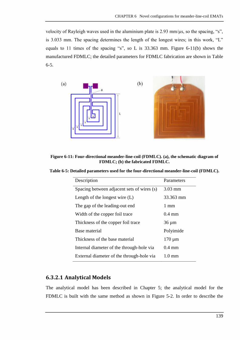
CHAPTER 6 Novel configurations for meander-line-coil EMATs
139
velocity of Rayleigh waves used in the aluminium plate is 2.93 mm/µs, so the spacing, “s”,
is 3.033 mm. The spacing determines the length of the longest wires; in this work, “L”
equals to 11 times of the spacing “s”, so L is 33.363 mm. Figure 6-11(b) shows the
manufactured FDMLC; the detailed parameters for FDMLC fabrication are shown in Table
6-5.
Figure 6-11: Four-directional meander-line-coil (FDMLC). (a), the schematic diagram of
FDMLC; (b) the fabricated FDMLC.
Table 6-5: Detailed parameters used for the four-directional meander-line-coil (FDMLC).
Description Parameters
Spacing between adjacent sets of wires (s) 3.03 mm
Length of the longest wire (L) 33.363 mm
The gap of the leading-out end 1 mm
Width of the copper foil trace 0.4 mm
Thickness of the copper foil trace 36 µm
Base material Polyimide
Thickness of the base material 170 µm
Internal diameter of the through-hole via 0.4 mm
External diameter of the through-hole via 1.0 mm
6.3.2.1 Analytical Models
The analytical model has been described in Chapter 5; the analytical model for the
FDMLC is built with the same method as shown in Figure 5-2. In order to describe the

CHAPTER 6 Novel configurations for meander-line-coil EMATs
140
FDMLC clearly, an approximated model is used as shown in Figure 6-12; this model is
symmetrical with the origin, the point O.
There are 12 wires perpendicular to the y-axis; these 12 wires form a VLMLC. Similarly,
another 12 wires, which are perpendicular to the x-axis, form another VLMLC. Each
VLMLC is capable of generating symmetrical Rayleigh waves in two directions. Hence,
the FDMLC, which can be viewed as two sets of VLMLC, is able to produce Rayleigh
waves in four directions. In addition, due to the benefit of VLMLC, the FDMLC are able
to suppress the side lobes and at the same time generate multiple-directional Rayleigh
waves.
Figure 6-12: The approximated configuration of the four-directional meander-line-coil
(FDMLC).
The calculated beam directivity along angles from -450 to 450 is shown in Figure 6-13; the
magnitude is normalised by the peak of the main lobe. As expected, the side lobes are
suppressed significantly. By calculation, for this FDMLC, the HPBW and the SSL are
18.70 and -14.62 dB respectively. Because the model is symmetrical with the origin, the
beam directivity within the range from 450 to 1350, from 1350 to -1350, and from -1350 to -
450, are the same as that within angles from -450 to 450.

CHAPTER 6 Novel configurations for meander-line-coil EMATs
141
Figure 6-13: The simulated beam directivity of the four-directional meander-line-coil
(FDMLC) EMAT.
6.3.2.2 Experimental Results
To verify the capacity of generating multiple-directional Rayleigh waves of the FDMLC, a
receiver is employed to receive the directly transmitted Rayleigh waves. The receiver used
was a 10 mm CLMLC; the distance between the transmitter (FDMLC) and the receiver
(CLMLC) is 250 mm. The receiver was located at 00, 900, 1800, and 2700 respectively. The
magnitude of the received Rayleigh waves is shown in Figure 6-14; from this image, the
magnitude of the Rayleigh waves received was from 0.06 volt to 0.07 volt. Ideally, the
amplitude of the Rayleigh waves should be the same, however, the difference exists
between the measured data due to experimental errors, which are within tolerance of this
work.
Figure 6-14: The magnitude of the received Rayleigh waves.
0
0.02
0.04
0.06
0.08
0 90 180 270
Mag
nit
ud
e(V
)
Angle (degree)
The magnitude of the Rayleigh waves
generated by FDMLC
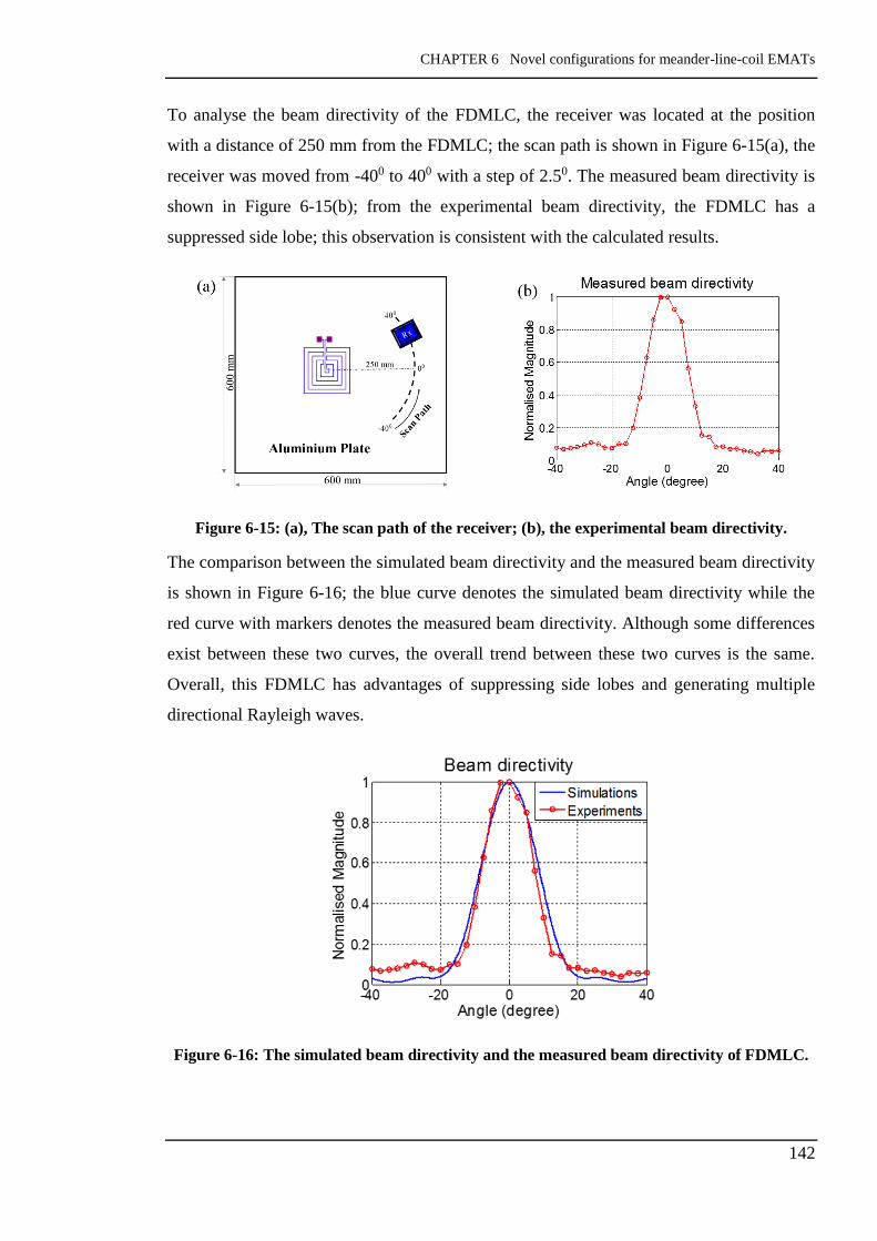
CHAPTER 6 Novel configurations for meander-line-coil EMATs
142
To analyse the beam directivity of the FDMLC, the receiver was located at the position
with a distance of 250 mm from the FDMLC; the scan path is shown in Figure 6-15(a), the
receiver was moved from -400 to 400 with a step of 2.50. The measured beam directivity is
shown in Figure 6-15(b); from the experimental beam directivity, the FDMLC has a
suppressed side lobe; this observation is consistent with the calculated results.
Figure 6-15: (a), The scan path of the receiver; (b), the experimental beam directivity.
The comparison between the simulated beam directivity and the measured beam directivity
is shown in Figure 6-16; the blue curve denotes the simulated beam directivity while the
red curve with markers denotes the measured beam directivity. Although some differences
exist between these two curves, the overall trend between these two curves is the same.
Overall, this FDMLC has advantages of suppressing side lobes and generating multiple
directional Rayleigh waves.
Figure 6-16: The simulated beam directivity and the measured beam directivity of FDMLC.

CHAPTER 6 Novel configurations for meander-line-coil EMATs
143
6.3.3 Six-directional Meander-line-coil (SDMLC) EMATs
The schematic diagram of the six-directional meander-line-coil (SDMLC) is shown in
Figure 6-17(a); “L” means the length of the longest wire; “s” means the spacing between
two adjacent wires; “g” means the gap of the leading-out end. In order to generate
Rayleigh waves, the spacing “s” is 3.033 mm, which is determined by the working
frequency, 483 kHz, and the Rayleigh waves’ velocity within the aluminium plate, 2.93
mm/µs. The length of the longest wire is determined; in this work, “L” is 19.261 mm. The
fabricated SDMLC is shown in Figure 6-17(b); the other parameters for the fabrication has
been clarified in Table 6-5.
Figure 6-17: Six-directional meander-line-coil (SDMLC). (a), the schematic diagram of
SDMLC; (b) the fabricated SDMLC.
6.3.3.1 Analytical Models
An approximated model for the SDMLC is shown in Figure 6-18; this model is
symmetrical with the origin, “O”. The SDMLC can be viewed as three sets of the VLMLC;
each set of the VLMLC contains 12 wires. Due to these three sets of the VLMLC, the
SDMLC is able to generate Rayleigh waves in 6 directions, which are along 00, 600, 1200,
1800, -1200, and -600 respectively.

CHAPTER 6 Novel configurations for meander-line-coil EMATs
144
Figure 6-18: The approximated model for the six-directional meander-line-coil (SDMLC).
The beam directivity of this approximated model of the SDMLC is shown in Figure 6-19,
which shows the normalised magnitude of the Rayleigh waves versus angles from -600 to
600. As expected, the maximum magnitude occurs at 00, -600 and 600 respectively. From -
300 to 300, the magnitude of Rayleigh waves is determined by the VLMLC along the angle,
00. For angles from -600 to -300 and from 300 to 600, the magnitude of Rayleigh waves is
determined by the other two sets of VLMLC which are along the angles 600 and 1200
respectively. The calculated HPBW and the SSL are 31.740 and -7.57 dB respectively.
Figure 6-19: The simulated beam directivity of the six-directional meander-line-coil (SDMLC)
EMAT
6.3.3.2 Experimental Results
Several experiments were conducted to study the beam property of the SDMLC. The
transmitter used was the SDMLC as clarified in Figure 6-17(b); the receiver used was the
-60 -40 -20 0 20 40 600
0.2
0.4
0.6
0.8
1
X: -30
Y: 0.1749
Beam directivity of SDMLC EMAT
Angle (degree)
Norm
alis
ed M
agnitude
X: 30
Y: 0.1749

CHAPTER 6 Novel configurations for meander-line-coil EMATs
145
same as that used in section 6.3.2.2. At a centre-to-centre distance of 250 mm from the
transmitter, the receiver was placed at 00, 600, 1200, 1800, 2400, and 3000 respectively to
verify the ability of generating multiple-directional Rayleigh waves. Figure 6-20 shows the
maximum magnitude of the received Rayleigh waves versus various angles; the received
amplitude was from 33 mV to 44 mV; possible reasons for the non-uniform amplitude are
the experimental noise, and possibly the errors due to the positioning of the receiver.
Figure 6-20: The magnitude of the received Rayleigh waves.
The beam directivity of the SDMLC was experimentally studied; the scan path is shown in
Figure 6-21(a). The receiver was moved from -400 to 400 at a distance of 250 mm from the
transmitter. The measured beam directivity of the SDMLC is shown in Figure 6-21(b). As
expected, the maximum magnitude of the received Rayleigh waves occurs at 00 and the
minimum magnitude occurs at -300 and 300. The amplitude of the received Rayleigh waves
increases from -300 to -400 and from 300 to 400 due to the effect of the other two sets of
VLMLC which are along the angles -600 and 600 respectively.
Figure 6-21: (a), The scan path of the receiver; (b), the experimental beam directivity.
0
0.01
0.02
0.03
0.04
0.05
0 60 120 180 240 300
Mag
nit
ud
e (V
)
Angle (degree)
The magnitude of Rayleigh waves
generated by SDMLC

CHAPTER 6 Novel configurations for meander-line-coil EMATs
146
The comparison between the calculated beam directivity and measured beam directivity of
the SDMLC is shown in Figure 6-22, where the blue curve denotes the simulated beam
directivity whereas the red curve denotes the measured beam directivity. The trend of the
simulated beam directivity shows a good agreement with that of the measured beam
directivity. Some differences exist between these two curves due to the inevitable
experimental error.
Figure 6-22: The simulated beam directivity and the measured beam directivity of SDMLC.
6.3.4 Discussion
Two novel meander-line-coil EMATs to generate multiple-directional Rayleigh waves are
proposed by the author for the first time; one is the four-directional meander-line-coil
(FDMLC) and the other one is the six-directional meander-line-coil (SDMLC). These
multiple-directional Rayleigh waves’ meander-line-coils can be viewed as several sets of
variable-length meander-line-coils (VLMLC), so multiple-directional Rayleigh waves’
meander-line-coils are capable of suppressing side lobes. The beam property of Rayleigh
waves generated by the multiple-directional meander-line-coil EMATs is studied
analytically and analysed experimentally. For the pulse-echo detection, due to the capacity
of generating multiple-directional Rayleigh waves, multiple-directional Rayleigh waves
meander-line-coil EMATs increase the monitoring area and improve the monitoring time.
6.4 Conclusions
In this chapter, several novel configurations for meander-line-coil EMATs are proposed by
the author for the first time. Firstly, a novel meander-line-coil, the VLMLC, is proposed
and studied. Both the simulated and experimental results suggest that the VLMLC has a

CHAPTER 6 Novel configurations for meander-line-coil EMATs
147
benefit of significantly suppressing side lobes of Rayleigh waves over the CLMLC. The
step of the VLMLC has a significant effect on the beam directivity of Rayleigh waves; a
larger step guarantees a lower SSL but slightly widens the HPBW of the main lobe.
On the basis of the VLMLC, two multiple-directional Rayleigh waves’ EMATs, the four-
directional meander-line-coil (FDMLC) and the six-directional meander-line-coil
(SDMLC), are proposed by the author. FDMLC and SDMLC can be viewed as several sets
of VLMLC; and therefore both of these coils are able to generate Rayleigh waves in
multiple directions and at the same time suppressing the side lobes. The multiple-
directional Rayleigh waves EMATs are advantageous in applications of inspecting large
samples. However, multiple-directional Rayleigh waves EMATs decrease the sensitivity of
flaw detection. Multiple-directional Rayleigh waves EMATs pose a possibility in the
future, that is combining multiple-directional EMATs and unidirectional EMATs together,
especially for large specimen detection; more specifically, multiple-directional EMATs can
be used to provide an initial estimation of the flaw location and unidirectional-EMATs can
be used to locate the flaw more precisely.

CHAPTER 7 Conclusions and recommendations for future work
148
Chapter 7 Conclusions and Recommendations for Future
Work
7.1 Conclusions
This thesis focuses on the meander-line-coil EMATs to generate Rayleigh waves based on
the Lorentz force mechanism. Although considerable works have been reported on the
study of meander-line-coil EMATs by means of simulations and experiments, there are
still many important issues, such as the radiation pattern and the beam features of Rayleigh
waves, which need further investigation. The overall aim of this work was to explore novel
efficient modelling techniques and novel configurations for meander-line-coil EMATs. To
achieve this aim, the author proposed two novel modelling methods for simulating
different planes of the test piece; the first method combines the analytical method and the
finite-different time-domain (FDTD) method for simulating the vertical plane of the
material (Chapter 4); the second method utilizes a wholly analytical model to simulate the
horizontal surface plane of the material (Chapter 5). The author further proposed three
novel configurations for meander-line-coil EMATs, the radiation patterns and beam
directivities of which were analytically studied with a wholly analytical model, and
validated by experiments (Chapter 6).
7.1.1 FDTD Method for Simulating US Behaviours
The FDTD solver, SimSonic [72], was further developed / adapted by the author for
simulating ultrasound behaviours, such as steering, focusing and scattering. Several
findings were made in Chapter 3:
1) The Hilbert Transformation and the FDTD method can be combined together to
produce the radiation pattern of ultrasound waves, which in turn can be used to analyse
the beam features.
2) The beam features in the full-field inspection were investigated; simulated results
revealed that, for the near field inspection, the focusing technique provides a better
beam directivity and a more concentrated beam intensity than the steering technique; for
the far field inspection, the steering technique is advantageous because the steering
technique requires less modelling time than the focusing technique, and at the same

CHAPTER 7 Conclusions and recommendations for future work
149
time provides a good beam directivity. Therefore, for a full-field inspection, the
focusing technique is normally used for near field inspections and the steering technique
is normally used for far field inspections; these numerical results based on FDTD
method were consistent with the analytical results presented in [69].
In addition, the FDTD method was used to model the scattering behaviours of ultrasound
waves; results revealed both the directly transmitted ultrasound waves and the scattered
ultrasound waves can be captured by the receiver. Overall, the study of FDTD provided a
solid foundation for the EMAT simulations introduced in Chapter 4.
7.1.2 Vertical Plane Modelling for EMATs
A novel modelling method combining the analytical method and the FDTD method
together to build EMAT models was proposed by the author for the first time, as described
in Chapter 4. This novel modelling method was a 2D simulation focusing on the vertical
plane of the material; the EM model was built by the adapted analytical method for
calculating Lorentz force densities, and the US modelling was carried out by the FDTD
method for simulating the propagation of ultrasound waves. There are a number of
conclusions drawn from the simulated and experimental results:
1) Because the coil used in this work was a meander-line-coil, the analytical solution to a
straight wire was needed. The strategy of adapting the analytical solution for a circular
coil to that for a straight wire was proposed by the author, and was validated by the
finite element method (FEM). Results revealed that the analytical solution to the straight
wire can be achieved by enlarging the radius of the circular coil; in addition, adapted
analytical solution was advantageous over FEM; both at a low frequency and at a high
frequency.
2) For the vertical plane modelling, the excitation signal used was a Gaussian-modulated
sinusoidal wave with a specific central frequency and a specific fractional bandwidth.
The effect of the fractional bandwidth of the excitation signal on the interference
behaviours of Rayleigh waves was investigated; results showed that, with a smaller
fractional bandwidth, the interference of Rayleigh waves was better. More specifically,
for the specific configuration EMAT used in this work, Rayleigh waves showed a good
interference with a fractional bandwidth equalling to or smaller than 0.3.

CHAPTER 7 Conclusions and recommendations for future work
150
3) The depth profile of Rayleigh waves, the radiation pattern, and the beam features of
Rayleigh waves indicated the Rayleigh waves are mainly concentrated in a depth within
one wavelength of Rayleigh waves. At a depth beyond one wavelength, Rayleigh waves
decreased by 80% or higher.
4) Experiments were conducted to validate the proposed modelling methods; by means of
the root-mean-square error (RMSE) and the correlation coefficient, experiments showed
a good agreement with simulations: the RMSE and the correlation coefficient between
experiments and simulations were 0.0834 and 0.9927 respectively.
5) Simulations and experiments showed that the attenuation of Rayleigh waves along the
surface of the material was very small; with a travelling distance of 5 cm, the
attenuation was 0.0034% from simulations and 0.0039% from experiments; this
observation further proved the capacity of Rayleigh waves for a long distance inspection.
6) The scattering behaviours of Rayleigh waves was studied by this novel modelling
method; results showed a good agreement between experiments and simulations; the
RMSE and the correlation coefficient for the scattering behaviour were 0.1159 and
0.9241 respectively. Further, unidirectional Rayleigh waves were modelled; the
Rayleigh waves signal was strengthened by 1.9849 in one direction while was
weakened by 0.2336 in the other direction; these results based on the proposed novel
modelling method were consistent with the numerical results presented in [23].
7.1.3 Surface Plane Modelling for EMATs
A novel modelling strategy based on a wholly analytical method was proposed by the
author for the first time, as described in Chapter 5. This novel modelling method was a 2D
simulation focusing on the surface plane of the material, and therefore it extended the 2D
simulations described in Chapter 4 to pseudo – 3D cases. Based on this novel modelling
method, the beam directivity of Rayleigh waves generated by meander-line-coil EMATs
were studied; some conclusions are presented below:
1) Based on the wholly analytical model, a main lobe and several side lobes of the
Rayleigh waves beam were observed for the conventional meander-line-coil EMATs;
the main lobe of the Rayleigh waves was along the normal direction of the meander-
line-coil, whereas the side lobes of Rayleigh waves radiated in undesirable directions.

CHAPTER 7 Conclusions and recommendations for future work
151
2) The effect of the length of the meander-line-coil on the radiation pattern of Rayleigh
waves was analytically studied; results showed that, with a larger length, the half
power beamwidth (HPBW) of the main lobe was smaller but the magnitude of sidelobe
level (SLL) was larger; with a length from 10 mm to 65 mm, the HPBW decreased by
82.32% but the SSL increases by 64.62%.
3) Experiments were carried out to study the beam directivity of Rayleigh waves and to
validate the proposed wholly analytical modelling method; experimental results
showed a good agreement with the simulated results, and therefore this novel
modelling method, focusing on the surface place of the material, is capable of
analysing the beam directivity of Rayleigh waves.
7.1.4 Novel Configurations for EMATs
Several novel configurations for meander-line-coil EMATs were proposed by the author
for the first time and described in Chapter 6. These novel meander-line-coil EMATs were
studied analytically and experimentally; some findings are presented below:
1) With the novel variable-length meander-line-coil (VLMLC), the side lobes of the beam
of Rayleigh waves, observed in the conventional constant-length meander-line-coil
(CLMLC), were significantly suppressed. However, the HPBW of the main lobe
increased slightly for VLMLC.
2) The effect of the step of the VLMLC on the radiation pattern of Rayleigh waves was
investigated; results revealed that, a larger step guaranteed a lower SSL but a larger
main lobe. For the 50 mm VLMLC with a step from 2 mm to 10 mm, the HPBW of the
main lobe increased by 18.16% and the SSL decreased by 92.95%.
3) Two multiple-directional Rayleigh waves meander-line-coil EMATs were proposed by
the author, the four-directional meander-line-coil (FDMLC) and the six-directional
meander-line-coil (SDMLC). From analytical and experimental studies, these EMATs
can be viewed as a combination of several sets of VLMLC, and therefore they were
capable of suppressing side lobes. In addition, experiments showed these novel
multiple-directional Rayleigh waves were capable of simultaneously generating
Rayleigh waves in four or six directions.

CHAPTER 7 Conclusions and recommendations for future work
152
7.2 Recommendations for Future Work
Based on the conclusions drawn from this study, future work is recommended to further
the study of EMATs.
1) For vertical plane modelling, as shown in Chapter 4, the EMAT-US model used was an
approximated model using only point sources (Lorentz force density) for generating
Rayleigh waves; a more detailed model, with volume sources (Lorentz force density)
within the skin depth, is worth considering in the future.
2) Throughout this study, the dynamic magnetic field generated by the meander-line-coil
was neglected due to the small excitation AC current. Although the effect of the
dynamic magnetic field is very small with a small excitation AC current, taking the
dynamic magnetic field into account will increase the precision of the calculation. It
should be noted that when the AC current is large, the dynamic magnetic field must be
considered as it is one of the mechanisms to generate ultrasound waves [39].
3) For EMAT scattering behaviours, as shown in section 4.7, only the scatter normal to
the surface was studied. It will be worth investigating the scattering behaviours of
scatters in other orientations as it is a variable in practical applications.
4) For the beam directivity measurement, as shown in Chapter 5 and Chapter 6, the
receiver used was a 10 mm-length meander-line-coil, which has its own radiation
pattern as a transmitter. In order to increase the spatial resolution of the received signal,
a miniature receiver should be used. [23] employed a miniature receiver, Pinducer,
which is a displacement sensor with elements of 0.053 inch diameters, to receive the
Rayleigh waves generated by the meander-line-coil EMATs; it is worthwhile trying
this miniature receiver in the future. In addition, the Pinducer is made of piezoceramic,
and therefore it poses a possibility of combining the conventional piezoelectric
transducers and the electromagnetic acoustic transducers (EMATs) together.
5) Several novel configurations for EMATs were proposed in this work; the optimal
parameters for such novel configurations of EMATs, such as the width of the wire and
the size of the permanent magnet, are worth investigating for the optimal design of
such sensors.
6) The multiple-directional Rayleigh waves EMATs proposed in section 6.3 are capable
of inspecting large specimens but with a low sensitivity of flaw detections. [23]
proposed a unidirectional Rayleigh waves EMATs as introduced in section 4.8. In

CHAPTER 7 Conclusions and recommendations for future work
153
practical applications, the capacity of combining the multiple-directional Rayleigh
waves EMATs to provide the initial estimation of the flaw location and the
unidirectional EMATs to locate the flaw precisely is worth investigating.
7) This study mainly focuses on the meander-line-coil EMATs operated on Lorentz force
mechanism for Rayleigh wave generation. However, the methodology for sensor
analysis and design can be extended to other type of EMATs; using this methodology
to investigate the property of bulk waves EMATs and Lamb waves EMATs can be a
focus in the future.
Extending from the work included in the thesis, one promising filed is the body inspection
with SV waves. As describe previously, the meander-line-coil is capable of generating
Rayleigh waves, longitudinal waves and shear vertical (SV) waves simultaneously, from
which SV waves have a large magnitude as Rayleigh waves, and therefore SV waves are
capable for body inspections. Based on the methodology proposed by the author, as shown
in Chapter 4, the property of SV waves generated by meander-line-coil EMATs can be
investigated. In addition, SV waves can be steered or focused with prescribed parameters,
such as the operational frequency and the spacing between two adjacent wires of the
meander-line-coil [22, 37]; the steering and focusing behaviours of SV waves can be
investigated by the modelling method proposed by the author. Further, the FDMLC and the
SDMLC are capable of generating SV waves in the material in multiple directions; these
multiple directional SV EMATs can be a design starting point for producing EMATs-SV
waves tomography in the future.

References
154
REFERENCES
[1] P. Cawley, "Ultrasonic measurements for the quantitative NDE of adhesive joints-
potential and challenges," in Ultrasonics Symposium, 1992. Proceedings., IEEE
1992, 1992, pp. 767-772.
[2] B. Chassignole, D. Villard, M. Dubuget, J. Baboux, and R. El Guerjouma,
"Characterization of austenitic stainless steel welds for ultrasonic NDT," in
REVIEW OF PROGRESS IN QUANTITATIVE NONDESTRUCTIVE
EVALUATION: Volume 19, 2000, pp. 1325-1332.
[3] B. Drinkwater and P. Cawley, "Measurement of the frequency dependence of the
ultrasonic reflection coefficient from thin interface layers and partially contacting
interfaces," Ultrasonics, vol. 35, pp. 479-488, 1997.
[4] B. W. Drinkwater and P. D. Wilcox, "Ultrasonic arrays for non-destructive
evaluation: A review," NDT & E International, vol. 39, pp. 525-541, 2006.
[5] J. Gallego-Juarez, "Piezoelectric ceramics and ultrasonic transducers," Journal of
Physics E: Scientific Instruments, vol. 22, p. 804, 1989.
[6] H. Jaffe and D. Berlincourt, "Piezoelectric transducer materials," Proceedings of
the IEEE, vol. 53, pp. 1372-1386, 1965.
[7] B. Jaffe, Piezoelectric ceramics vol. 3: Elsevier, 2012.
[8] A. Arnau, Piezoelectric transducers and applications vol. 2004: Springer, 2004.
[9] R. Ribichini, "Modelling of electromagnetic acoustic transducers," Doctor of
Philosophy, Department of Mechanical Engineering, Imperial Colledge London,
2011.
[10] Y. Xie, W. Yin, Z. Liu, and A. Peyton, "Simulation of ultrasonic and EMAT arrays
using FEM and FDTD," Ultrasonics, vol. 66, pp. 154-165, 2016.
[11] H. Gao, S. Ali, B. Lopez, and P. Lopez, "New developments in EMAT techniques
for surface inspection," in REVIEW OF PROGRESS IN QUANTITATIVE
NONDESTRUCTIVE EVALUATION: VOLUME 32, 2013, pp. 902-908.
[12] D. W. Blodgett and K. C. Baldwin, "Laser-based ultrasonics: Applications at APL,"
Johns Hopkins APL technical digest, vol. 26, pp. 36-45, 2005.
[13] Y. Xie, S. Rodriguez, W. Zhang, Z. Liu, and W. Yin, "Simulation of an
Electromagnetic Acoustic Transducer Array by using Analytical method and
FDTD," Journal of Sensors, vol. 501, p. 5451821, 2016.
[14] Y. Xie, L. Yin, R. G. Sergio, T. Yang, Z. Liu, and W. Yin, "A wholly analytical
method for the simulation of an electromagnetic acoustic transducer array,"
International Journal of Applied Electromagnetics and Mechanics, pp. 1-15, 2016.
[15] Y. Xie, L. Yin, Z. Liu, P. Deng, and W. Yin, "A Novel Variable-Length Meander-
line-Coil EMAT for Side Lobe Suppression," IEEE Sensors Journal, vol. PP, 2016.
[16] M. Hirao and H. Ogi, EMATs for science and industry: noncontacting ultrasonic
measurements: Springer Science & Business Media, 2003.
[17] E. C. Ashigwuike, "Coupled Finite Element Modelling and Transduction Analysis
of a Novel EMAT Configuration Operating on Pipe Steel Materials," Brunel
University London, 2014.
[18] S. Huang, S. Wang, W. Li, and Q. Wang, "Electromagnetic Ultrasonic Guided
Waves," ed: Springer, 2016.

References
155
[19] R. Ribichini, "MODELLING OF ELECTROMAGNETIC ACOUSTIC
TRANSDUCERS (Ph.D. Dissertation)," Ph.D. Dissertation, Imperial College
London, 2011.
[20] R. N. Thurston and A. D. Pierce, Ultrasonic measurement methods vol. 19:
Elsevier, 1990.
[21] X. Jian, S. Dixon, K. Quirk, and K. Grattan, "Electromagnetic acoustic transducers
for in-and out-of plane ultrasonic wave detection," Sensors and Actuators A:
Physical, vol. 148, pp. 51-56, 2008.
[22] H. Ogi, M. Hirao, and T. Ohtani, "Line-focusing of ultrasonic SV wave by
electromagnetic acoustic transducer," The Journal of the Acoustical Society of
America, vol. 103, pp. 2411-2415, 1998.
[23] S. Wang, R. Su, X. Chen, L. Kang, and G. Zhai, "Numerical and experimental
analysis of unidirectional meander-line coil electromagnetic acoustic transducers,"
Ultrasonics, Ferroelectrics, and Frequency Control, IEEE Transactions on, vol. 60,
pp. 2657-2664, 2013.
[24] D. Jiles, "Introduction to magnetism and magnetic materials," 1998.
[25] S. Huang and S. Wang, "New Technologies in Electromagnetic Non-destructive
Testing," ed: Springer, 2016.
[26] S. Dixon, R. Edwards, and X. Jian, "Inspection of rail track head surfaces using
electromagnetic acoustic transducers (EMATs)," Insight-Non-Destructive Testing
and Condition Monitoring, vol. 46, pp. 326-330, 2004.
[27] X. Jian, S. Dixon, and R. S. Edwards, "Ultrasonic generation and optimization for
EMAT," in REVIEW OF PROGRESS IN QUANTITATIVE NONDESTRUCTIVE
EVALUATION, 2005, pp. 1041-1046.
[28] X. Jian, S. Dixon, K. Grattan, and R. S. Edwards, "A model for pulsed Rayleigh
wave and optimal EMAT design," Sensors and Actuators A: Physical, vol. 128, pp.
296-304, 2006.
[29] H.-J. Salzburger, F. Niese, and G. Dobmann, "EMAT pipe inspection with guided
waves," Welding in the world, vol. 56, pp. 35-43, 2012.
[30] P. Wilcox, M. Lowe, and P. Cawley, "Omnidirectional guided wave inspection of
large metallic plate structures using an EMAT array," Ultrasonics, Ferroelectrics,
and Frequency Control, IEEE Transactions on, vol. 52, pp. 653-665, 2005.
[31] R. Ribichini, F. Cegla, P. B. Nagy, and P. Cawley, "Study and comparison of
different EMAT configurations for SH wave inspection," Ultrasonics,
Ferroelectrics, and Frequency Control, IEEE Transactions on, vol. 58, pp. 2571-
2581, 2011.
[32] I. T. Inc. (2016). EMAT Technology. Available:
http://innerspec.com/knowledge/emat-technology
[33] S. Huang, Z. Wei, W. Zhao, and S. Wang, "A new omni-directional EMAT for
ultrasonic Lamb wave tomography imaging of metallic plate defects," Sensors, vol.
14, pp. 3458-3476, 2014.
[34] L. Kang, S. Wang, Z. Li, and G. Zhai, "Optimal design of surface wave emats for
enhancing their ultrasonic signal strength," The Journal of the Acoustical Society of
America, vol. 131, pp. 3466-3466, 2012.
[35] Z. Liu, Y. Hu, J. Fan, W. Yin, X. Liu, C. He, and B. Wu, "Longitudinal mode
magnetostrictive patch transducer array employing a multi-splitting meander coil
for pipe inspection," NDT & E International, vol. 79, pp. 30-37, 2016.
References
156
[36] H. Ogi, M. Hirao, and T. Ohtani, "Flaw detection by line-focusing electromagnetic
acoustic transducers," in Ultrasonics Symposium, 1997. Proceedings., 1997 IEEE,
1997, pp. 653-656.
[37] H. Ogi, M. Hirao, and T. Ohtani, "Line-focusing electromagnetic acoustic
transducers for the detection of slit defects," Ultrasonics, Ferroelectrics, and
Frequency Control, IEEE Transactions on, vol. 46, pp. 341-346, 1999.
[38] W. Shujuan, L. Zhichao, K. Lei, H. Xiaoguang, and Z. Xiao, "Modeling and
comparison of three bulk wave EMATs," in IECON 2011-37th Annual Conference
on IEEE Industrial Electronics Society, 2011, pp. 2645-2650.
[39] S. Wang, L. Kang, Z. Li, G. Zhai, and L. Zhang, "3-D modeling and analysis of
meander-line-coil surface wave EMATs," Mechatronics, vol. 22, pp. 653-660, 2012.
[40] R. Edwards, A. Sophian, S. Dixon, G.-Y. Tian, and X. Jian, "Dual EMAT and PEC
non-contact probe: applications to defect testing," NDT & E International, vol. 39,
pp. 45-52, 2006.
[41] R. S. Edwards, S. Dixon, and X. Jian, "Characterisation of defects in the railhead
using ultrasonic surface waves," NDT & E International, vol. 39, pp. 468-475,
2006.
[42] M. Hirao and H. Ogi, "Electromagnetic acoustic resonance and materials
characterization," Ultrasonics, vol. 35, pp. 413-421, 1997.
[43] K. Hao, S. Huang, W. Zhao, S. Wang, and J. Dong, "Analytical modelling and
calculation of pulsed magnetic field and input impedance for EMATs with planar
spiral coils," NDT & E International, vol. 44, pp. 274-280, 2011.
[44] X. Jian and S. Dixon, "Enhancement of EMAT and eddy current using a ferrite
back-plate," Sensors and Actuators A: Physical, vol. 136, pp. 132-136, 2007.
[45] L. Kang, S. Dixon, K. Wang, and J. Dai, "Enhancement of signal amplitude of
surface wave EMATs based on 3-D simulation analysis and orthogonal test
method," NDT & E International, vol. 59, pp. 11-17, 2013.
[46] K. Mirkhani, C. Chaggares, C. Masterson, M. Jastrzebski, T. Dusatko, A. Sinclair,
R. J. Shapoorabadi, A. Konrad, and M. Papini, "Optimal design of EMAT
transmitters," NDT & E International, vol. 37, pp. 181-193, 2004.
[47] P. J. Shull, Nondestructive evaluation: theory, techniques, and applications: CRC
press, 2002.
[48] H. Gao, S. Ali, and B. Lopez, "Austenitic Weld Inspection with EMAT Phased
Array," 2010.
[49] H. Gao and B. Lopez, "Development of single-channel and phased array
electromagnetic acoustic transducers for austenitic weld testing," Mater Eval, vol.
68, pp. 821-7, 2010.
[50] M.-I. Rocha-Gaso, C. March-Iborra, Á. Montoya-Baides, and A. Arnau-Vives,
"Surface generated acoustic wave biosensors for the detection of pathogens: A
review," Sensors, vol. 9, pp. 5740-5769, 2009.
[51] K.-J. Langenberg, R. Marklein, and K. Mayer, Ultrasonic nondestructive testing of
materials: theoretical foundations: CRC Press, 2012.
[52] I. A. Viktorov, Rayleigh and Lamb waves: physical theory and applications:
Plenum press, 1970.
[53] E. A. Ash and E. G. Paige, Rayleigh-Wave Theory and Application: Proceedings of
an International Symposium Organised by The Rank Prize Funds at The Royal
Institution, London, 15–17 July, 1985 vol. 2: Springer Science & Business Media,
2012.

References
157
[54] U. o. Oslo, "An introduction to surface waves," ed, 2004.
[55] D. Ensminger and L. J. Bond, Ultrasonics: fundamentals, technologies, and
applications: CRC press, 2011.
[56] J. K. Na and J. L. Blackshire, "Interaction of Rayleigh surface waves with a tightly
closed fatigue crack," NDT & E International, vol. 43, pp. 432-439, 2010.
[57] M. Silk, "The determination of crack penetration using ultrasonic surface waves,"
NDT international, vol. 9, pp. 290-297, 1976.
[58] Z. Su and L. Ye, Identification of damage using Lamb waves: from fundamentals to
applications vol. 48: Springer Science & Business Media, 2009.
[59] D. N. Alleyne and P. Cawley, "Optimization of Lamb wave inspection techniques,"
NDT & E International, vol. 25, pp. 11-22, 1992.
[60] D. N. Alleyne and P. Cawley, "The interaction of Lamb waves with defects,"
Ultrasonics, Ferroelectrics, and Frequency Control, IEEE Transactions on, vol. 39,
pp. 381-397, 1992.
[61] L. Kang, S. Wang, T. Jiang, and G. Zhai, "Optimal design of Lamb wave
electromagnetic acoustic transducers for improving their excitation performance,"
Japanese Journal of Applied Physics, vol. 50, p. 07HD01, 2011.
[62] G. Zhai, T. Jiang, L. Kang, and S. Wang, "Minimizing influence of multi-modes
and dispersion of electromagnetic ultrasonic lamb waves," Ultrasonics,
Ferroelectrics, and Frequency Control, IEEE Transactions on, vol. 57, pp. 2725-
2733, 2010.
[63] S. Wang, L. Kang, Z. Li, G. Zhai, and L. Zhang, "A novel method for modeling
and analysis of meander-line-coil surface wave EMATs," in Life System Modeling
and Intelligent Computing, ed: Springer, 2010, pp. 467-474.
[64] S. Wang, Z. Li, L. Kang, and G. Zhai, "Influence of Coil Parameters on Rayleigh
Waves Excited by Meander-Line Coil EMATs," in Intelligent Computing for
Sustainable Energy and Environment, ed: Springer, 2013, pp. 94-103.
[65] R. Dhayalan and K. Balasubramaniam, "A hybrid finite element model for
simulation of electromagnetic acoustic transducer (EMAT) based plate waves,"
NDT & E International, vol. 43, pp. 519-526, 2010.
[66] R. Dhayalan and K. Balasubramaniam, "A two-stage finite element model of a
meander coil electromagnetic acoustic transducer transmitter," Nondestructive
Testing and Evaluation, vol. 26, pp. 101-118, 2011.
[67] M. Eskandarzade, T. Kundu, N. Liebeaux, D. Placko, and F. Mobadersani,
"Numerical simulation of electromagnetic acoustic transducers using distributed
point source method," Ultrasonics, vol. 50, pp. 583-591, 2010.
[68] D. Placko and T. Kundu, DPSM for modeling engineering problems: John Wiley &
Sons, 2007.
[69] L. Azar, Y. Shi, and S.-C. Wooh, "Beam focusing behavior of linear phased
arrays," NDT & E International, vol. 33, pp. 189-198, 2000.
[70] D. E. Bray and R. K. Stanley, Nondestructive evaluation: a tool in design,
manufacturing and service: CRC press, 1996.
[71] L. Bos and M. A. Slawinski, "Elastodynamic equations: characteristics, wavefronts
and rays," The Quarterly Journal of Mechanics and Applied Mathematics, vol. 63,
pp. 23-38, 2010.
[72] E. Bossy, "SimSonic Suite User’s guide for SimSonic3D," 2012.
[73] G. D. Smith, Numerical solution of partial differential equations: finite difference
methods: Oxford university press, 1985.

References
158
[74] R. Yan, Base wavelet selection criteria for non-stationary vibration analysis in
bearing health diagnosis: ProQuest, 2007.
[75] J.-C. Hong, K. H. Sun, and Y. Y. Kim, "The matching pursuit approach based on
the modulated Gaussian pulse for efficient guided-wave damage inspection," Smart
Materials and Structures, vol. 14, p. 548, 2005.
[76] S.-C. Wooh and Y. Shi, "Optimum beam steering of linear phased arrays," Wave
motion, vol. 29, pp. 245-265, 1999.
[77] S.-C. Wooh and Y. Shi, "A simulation study of the beam steering characteristics for
linear phased arrays," Journal of nondestructive evaluation, vol. 18, pp. 39-57,
1999.
[78] M. Weston, "Advanced Ultrasonic Digital Imaging and Signal Processing for
Applications in the Field of Non-Destructive Testing," 2012.
[79] C. Dodd and W. Deeds, "Analytical Solutions to Eddy‐Current Probe‐Coil
Problems," Journal of applied physics, vol. 39, pp. 2829-2838, 1968.
[80] X. Chen, R. Su, H. Zhang, S. Wang, and G. Zhai, "Influence of coil parameters on
transduction performance of unidirectional EMATs for Rayleigh wave," in
Nondestructive Evaluation/Testing: New Technology & Application (FENDT),
2013 Far East Forum on, 2013, pp. 150-154.
[81] N. Haskell, "Radiation pattern of surface waves from point sources in a multi-
layered medium," Bulletin of the Seismological Society of America, vol. 54, pp.
377-393, 1964.
[82] N. Haskell, "Radiation pattern of Rayleigh waves from a fault of arbitrary dip and
direction of motion in a homogeneous medium," Bulletin of the Seismological
Society of America, vol. 53, pp. 619-642, 1963.
[83] A. Love, "H. A treatise on the mathematical theory of elasticity," Cambridge:
Cambridge University Press, vol. 1, p. 952, 1944.
[84] R. Dhayalan, V. S. N. Murthy, C. Krishnamurthy, and K. Balasubramaniam,
"Improving the signal amplitude of meandering coil EMATs by using ribbon soft
magnetic flux concentrators (MFC)," Ultrasonics, vol. 51, pp. 675-682, 2011.
[85] Z. Li, W. Zhai, R. Su, and L. Kang, "Coil parameter analysis of meander-line coil
electromagnetic acoustic transducer-based Rayleigh waves," Transactions of the
Institute of Measurement and Control, p. 0142331213499808, 2013.
[86] S. Wang, P. Xin, L. Kang, and G. Zhai, "Research on influence of lorentz force
mechanism on EMAT's transduction efficiency in steel plate," in Industrial
Electronics and Applications (ICIEA), 2010 the 5th IEEE Conference on, 2010, pp.
196-201.
[87] Z. Wei, S. Huang, S. Wang, and W. Zhao, "Magnetostriction-Based Omni-
Directional Guided Wave Transducer for High-Accuracy Tomography of Steel
Plate Defects," Sensors Journal, IEEE, vol. 15, pp. 6549-6558, 2015.