modelling short-scale variability and uncertainty during mineral resource estimation using a novel...

Modelling Short-Scale Variability and Uncertainty DuringMineral Resource Estimation Using a Novel Fuzzy EstimationTechnique

Khan Muhammad (1)* and Hylke J. Glass (2)

(1) Department of Mining Engineering, University of Engineering and Technology, Peshawar, KPK 25000, Pakistan(2) Camborne School of Mines, University of Exeter, Penryn, Cornwall TR10 9EZ, UK* Corresponding author. e-mail: [email protected]

For mineral resource assessment, techniques basedon fuzzy logic are attractive because they arecapable of incorporating uncertainty associated withmeasured variables and can also quantify theuncertainty of the estimated grade, tonnage etc. Thefuzzy grade estimation model is independent of thedistribution of data, avoiding assumptions andconstraints made during advanced geostatisticalsimulation, e.g., the turning bands method. Initially,fuzzy modelling classifies the data using all thecomponent variables in the data set. We adopt anovel approach by taking into account the spatialirregularity of mineralisation patterns using theGustafson–Kessel classification algorithm. Theuncertainty at the point of estimation was derivedthrough antecedent memberships in the input space(i.e., spatial coordinates) and transformed onto theoutput space (i.e., grades) through consequentmembership at the point of estimation. Rather thanprobabilistic confidence intervals, this uncertaintywas expressed in terms of fuzzy memberships, whichindicated the occurrence of mixtures of differentmineralogical phases at the point of estimation.Data from different sources (other than grades)could also be utilised during estimation. Applicationof the proposed technique on a real data set gaveresults that were comparable to those obtained froma turning bands simulation.

Keywords: uncertainty, method development, estimation,fuzzy logic, Gustafson–Kessel.

Received 21 May 09 – Accepted 27 Nov 09

Pour l’évaluation des ressources minérales, lestechniques basées sur la logique floue sont attrayantescar elles sont capables d’incorporer l’incertitudeassociée à des variables mesurées et permettent ausside quantifier l’incertitude de la teneur estimée, dutonnage etc. Le modèle d’estimation floue de la teneurest indépendant de la distribution des données, etévite les hypothèses et les contraintes faites au cours desimulations géostatistiques avancées, comme parexemple, dans le cas de la méthode des bandestournantes. Initialement la modélisation floue classe lesdonnées en utilisant toutes les variables de l’ensemblede données. Nous adoptons une nouvelle approche entenant compte de l’irrégularité spatiale des types deminéralisation en utilisant l’algorithme de classificationGustafson–Kessel. L’incertitude sur le pointd’estimation est obtenue au travers de l’appartenancedes précédents dans l’espace d’entrée (c.à.d. lescoordonnées spatiales) et transformée dans l’espacede sortie (c.à.d. les teneurs) au travers del’appartenance conséquente au point d’estimation.Plutôt que par des intervalles de confianceprobabiliste, cette incertitude est exprimée en termesd’adhésion floue, qui indique la présence de mélangesde différentes phases minéralogiques au pointd’estimation. Les données provenant de différentessources (autres que les teneurs) peuvent égalementêtre utilisés lors de l’estimation. L’application de latechnique proposée à des données réelles a donnédes résultats qui sont comparables à ceux obtenus àpartir d’une simulation de bandes tournantes.

Mots-clés : incertitude, développement de méthode,estimation, logique floue, Gustafson–Kessel.

Vol. 35 – N� 30911 p . 3 6 9 – 3 8 5

doi: 10.1111/j.1751-908X.2010.00051.xª 2011 The Authors. Geostandards and Geoanalytical Research ª 2011 International Association of Geoanalysts 3 6 9

For risk management in mineral resource estimation,variability and uncertainty (ISO 1993) are essential to con-sider, and can be characterised by the following quota-tions: ‘variability represents heterogeneity’ in a depositwhile ‘uncertainty represents partial ignorance on the partof the analyst’ (Anderson and Hattis 1999). Mann (1994)divides the types of uncertainties in geological modellinginto three main categories. The first type of uncertainty asso-ciated with errors in the measurement devices, techniquesetc., is routinely ignored in geostatistical estimation tech-niques. The second type of uncertainty is the variability orprobabilistic uncertainty in a deposit. This type of uncer-tainty is well-explained by geostatistical estimation tech-niques. Mann (1994) states that the third type ofuncertainty, associated with model parameters (e.g., fittingvariogram model to experimental semivariogram, regres-sion model to data etc.) will persist with any model as it isimpossible to estimate the accuracy of models.

Conditional simulations (Journel and Huijbregts 1978)are standard techniques used in the industry for determin-ing short-scale variability and uncertainty associated withthe estimated variable. However, these techniques are notfree from the shortcomings of traditional kriging techniquesand depend on original sample histogram and variogramsthat are sensitive to the sampling pattern and the numberof available samples. To overcome such shortcomings,novel techniques based on fuzzy logic (Zadeh 1965) haveemerged. A basic tool for expressing uncertainty in terms offuzzy logic is the membership value. Fuzzy membershipcomprises values ranging between 0 and 1 (inclusive),expressing the possibility or degree of truth of an event,e.g., the degree of membership to a particular mineralisa-tion. A crisp membership uij can only classify samples intotwo disjoint classes, e.g., any jth sample that entirelybelongs (when uij = 1) or does not belong (uij = 0) to anith mineralisation. Thus, the uncertainty in classification orthe possibility that a sample may represent two or moreclasses is not taken into account. Whilst a fuzzy member-ship lij of any jth sample can also quantify the possibilitythat a sample partially belongs to a particular mineralisa-tion (0 < lij < 1). In this way fuzzy logic can incorporate thefirst type of uncertainty, i.e., associated with preliminarydata, such as errors in measurement, core logging etc., inmineral resource estimation (Bárdossy and Fodor 2001).Bardossy et al. (1990) used fuzzy memberships that tookinto account the third type of uncertainty associated with fit-ting a variogram model and proposed a fuzzy krigingtechnique. Bárdossy and Fodor (2005) showed, in terms offuzzy memberships, that the uncertainty in estimation of ton-nage, grade and thickness parameters decreases as explo-ration progresses. Luo and Dimitrakopoulos (2003)

presented a mineral favourability index, combining knowl-edge from different sources by fuzzy logic reasoning, forresource estimation.

Robust fuzzy classification approaches, insensitive tosample distribution, can be used to identify patterns in data(Kaufman and Rousseuw 1990, Huber and Ronchetti2009). Heuristic classification techniques (Huber and Ron-chetti 2009) minimise an objective function; since the opti-misation in such case is a non-linear process therefore afeasible solution is achieved iteratively.

Limited fuzzy data-driven models (Pham 1997, Grima2000, Tutmez et al. 2007) have been previously devel-oped for mineral resource estimation. However, in theseprevious approaches, the algorithms used in the first step,i.e., the classification of samples, do not account for theirregular spatial distribution of the identified grade clas-ses ⁄ mineralisation. In this paper we show that the use ofGustafson–Kessel (GK) algorithm (Gustafson and Kessel1979) can improve previous classifications for fuzzy gradeestimation. Moreover, for estimating the influence of specificmineralisation, the previous models approximate the ante-cedent membership at the point of estimation by Gaussianmembership function only. A modified antecedent member-ship is presented, which is based on an adaptive distancenorm known as the Mahalanobis distance (Babuska andVerbruggen 1997, Babuska 1998) and a search neigh-bourhood around a point of estimation.

In the next sections, a brief background of data-drivenmodels for mineral resource estimation is discussed. Next,the potential of fuzzy models for estimating short-scale vari-ability in a deposit is analysed and compared with turningbands simulation. The steps of the proposed technique areexplained with a short example that emphasises theadvantage of GK classification algorithm over FuzzyC-Means (FCM) (Bezdek et al. 1984) classification. Finally,the results from application of the proposed technique onthe real data set are compared with output from turningbands conditional simulation.

Fuzzy modelling for grade prediction:Data-driven approach

Fuzzy modelling has the potential to incorporate type1, type 2 and type 3 uncertainties discussed earlier dur-ing mineral resource estimation. Two main approachesare used to integrate knowledge (knowledge-basedapproach) and data (data-driven approach) in fuzzymodels (Babuska 1998). First the input and output vari-ables are identified from the variables of the samples.

3 7 0 ª 2011 The Authors. Geostandards and Geoanalytical Research ª 2011 International Association of Geoanalysts

Knowledge-based systems collect a knowledge database from experts a priori. The increase in the amount ofa priori data and information requires a large number ofrules in the knowledge-based approach. By contrast,data-driven approaches are independent of any a prioriknowledge. Data-driven fuzzy models objectively classifydata using self learning fuzzy classification algorithms inCartesian product space (defined by xyz coordinates)(Babuska and Verbruggen 1997). Classification identifiesthe class centres and patterns of different types of miner-alisation, within the input space. Second, the possibility ofa point of estimation to belong to more then one miner-alogical phases is quantified by approximating fuzzymemberships in the input space. Such membershipsassociated with the input variables are called antecedentmemberships.

Third, the fuzzy inference system (FIS) approximatesthe cause and effect relationship between various inputvariables using fuzzy IF-THEN rules through intuitive logi-cal reasoning aided by logical operators (e.g., AND, ORetc.) within each rule. Each rule represents a specificgrade ⁄ geological class; therefore, choosing the numberof classes is as important as rule generation. The num-ber of classes can be validated by cluster validity mea-sures (Bezdek 1981) or other model-based clusteringtechniques (Fraley and Raftery 2002). The output mem-bership from the logical operators is produced in theoutput variable space. Each rule is identified by its ante-cedent and consequent part. The antecedent part ofeach rule lies between IF and THEN in the rule state-ment and defines the relationship between input vari-ables using logical operations (Babuska 1998). The

Figure 1. Four-step fuzzy grade estimation model for three types of mineralisation or grade zones.

ª 2011 The Authors. Geostandards and Geoanalytical Research ª 2011 International Association of Geoanalysts 3 7 1

consequent part of rule is the post-THEN part obtainedafter applying logical operations on antecedent mem-berships. The resulting consequent memberships quantifythe uncertainty associated with the corresponding outputvariable in terms of fuzzy memberships. The Mamdani(Pham 1997, Grima 2000) and Takagi Sugeno (TS)(Babuska 1998, Grima 2000, Tutmez et al. 2007) mod-els are popular inference models. A Mamdani typeinference model has both antecedent and consequentparts in terms of fuzzy propositions, whilst in the TSmodel the antecedent part is a fuzzy proposition andthe consequent part is a crisp function of the antecedentvariables. Figure 1 describes previous data-drivenMamdani (Pham 1997) and TS model (Grima 2000,Tutmez et al. 2007) types for grade estimation as afour-step fuzzy modelling approach.

For evaluation purposes a single crisp (defuzzified)value is often required for the output variable. An equationof weighted fuzzy mean defuzzification, widely usedbecause of its simplicity, is shown in Figure 1 where ai isthe degree of truth for the ith rule and giðx0; y0Þis the esti-mated grade output from ith rule of TS or Mamdani infer-ence models.

Estimating short-scale variabilityin a deposit

Turning bands method

Conditional simulations based on geostatistical tech-niques are traditionally used for determining the short-scale variation within the deposit. Because of its computa-tional efficiency for simulating values in three dimensions,the turning bands method (Journel and Huijbregts 1978,Chilès and Delfiner 1999) is widely applied in the miningindustry.

As the simulated values honour the original histo-gram and variogram in the Gaussian space, erroneousconstruction of these characteristic plots will propagateerrors in the simulations. While any bias in the samplingprocedure induces bias in the histogram, a correctedhistogram can be obtained by weighting with decluster-ing weights (Deutsch and Journel 1998). Furthermore,the mean of the deposit is assumed constant during thesimulation; in the case of a trend, such an assumption isnot valid. Although a number of simulated realisationsare produced, one cannot identify the realisation, match-ing the true distribution. The technique is also purely sta-tistical and independent of any geological or gradepatterns.

Fuzzy modelling

Fuzzy modelling has the potential to deal with model-ling non-linear and dynamic processes. The input (e.g., spa-tial coordinates) and output variables (e.g., grade asconcentration of a measured quantity) are identified fromthe available data. The short-scale variation can beapproximated through a two-step approach: first, the num-ber of mineralisation or grade classes such as high, med-ium and low grade zones, and their shape are identifiedusing the GK classification algorithms. For application ofthe TS model, smooth regression surfaces are derived foreach grade type. These define relationships between inputvariables (spatial coordinates) and output variables (grade)taking into account the memberships to correspondinggrade type obtained from the classification. Second, theuncertainty at the point of estimation is approximated interms of fuzzy memberships, which represent phases ofmineralisation, using fuzzy IF-THEN rules. The final grades,in terms of crisp values, are estimated by weighted averag-ing of the crisp values, obtained from the smooth regres-sion surfaces for each class ⁄ mineralisation.

A combination of different sources of information suchas type of mineralisation and distances of the known pointsfrom the point of estimation, their degree of membership toa particular type of mineralisation are combined by intui-tive fuzzy reasoning using the input and output variablesbased on IF-THEN rules. Fuzzy modelling techniques areindependent of constraints such as the minimum number ofsample pairs needed for variogram models, correctionsneeded for clustered sampling before simulation andstationary assumptions required in geostatistical models. Inconditional simulations, the uncertainty of estimation isexpressed by probabilistic confidence intervals from simu-lated values using number of realisations, whilst fuzzy mod-elling approximates the uncertainty in terms of fuzzymemberships.

Modified fuzzy model for measuringshort-scale variability

Grima (2000) used subtractive clustering (Chiu 1994)for classification. Pham (1997) and Tutmez et al. (2007)used the FCM algorithm for the classification of thesamples. All the classification approaches in the previousfuzzy models for grade prediction used Euclideandistances (i.e., distances between samples and class cen-tres are defined as sum of squares of the differencesbetween corresponding variables of the sample and classcentres) in the Cartesian space (xyz coordinate system) to


determine the similarity between a sample and a classcentre. Such classification gives equal weighting to thesquared difference components whilst determining the dis-tance between samples and class centres. However, it isimportant to know the irregular spread of the grade clas-ses ⁄ type of mineralisation and the direction of continuityof each mineralisation. Such information can be utilisedfurther when deriving antecedent memberships. A modi-fied fuzzy estimation model (Figure 2) is presented whichcan incorporate data from different sources to estimatethe short-scale variability.

The ‘p’ dimensional input variables xj1…. xjp represent-ing spatial coordinates for jth sample and the correspond-ing output variable grade ‘gj’ are identified andconcatenated in a single matrix.

X ¼

x11 ::: x1p g1: : : :: : : :

xN1 : xNp gN

��

��ð1Þ

The (N · p + 1) matrix X, where N is the number ofsamples, is classified into ‘c’ number of classes in the

Cartesian product space using iterative classification algo-rithm. The first step of the proposed technique is to use GKalgorithm (Figure 3) for classification. This is described indetail in the next section.

Gustafson–Kessel (GK) classificationalgorithm

The GK algorithm is an extended form of the FCMalgorithm. The architecture of GK and FCM algorithm is thesame because the optimisation is achieved by minimisingan objective function. If the distance of any jth sample fromthe ith grade ⁄ geological class vi is denoted by a distancedij, and its membership value by uij then the objective func-tion measure J is given by Equation (2)

J ¼XNi¼1

Xc

j¼1

umij d2

ij ð2Þ

The term c represents number of classes, m thefuzziness index and N the total number of samples. Thedissimilarity of a sample from a class centre during the iter-ative classification process is calculated by a suitable dis-tance measure. A fuzziness index value can be chosenbetween 1 and ¥ to represent the intensity of fuzziness inIdentify input (spatial coordinate) and

output variables (grade, mineralisation,geotechnical parameters)

Classify multivariate samples(input and output variables)

by applying the GK algorithm

Derive consequent regressionparameters using membershipsfrom the GK classification based

on TS model

Derive antecedent memberships(in the input space) from the available

information i.e., class-specific Mahalanobisdistances and memberships of the samples

within the search neighbourhood

Defuzzification

Derive consequent membershipsby combining antecedent memberships

using logical reasoning in fuzzyIF-THEN rules

Figure 2. The modified fuzzy grade prediction model.

Initialise class centre values and fuzzymemberships of samples (at t = 0)

Start iteration for t = 1 to max-iter

Update class centres using membershipsfrom previous iteration (using Eqn. 3)

Update fuzzy covariance matrix(Eqns 4a and 4b)

Calculate Mahalanobis distance (Eqn. 4)

Update memberships (Eqn. 5)

Calculate Maxdiff (Eqn. 6)

t = t + 1

t ≥ max-iter

MaxDiff ≤ ∈

Final cluster centresand memberships

False

True

True

False

End of the algorithm

Figure 3. Steps of the GK classification algorithm.


the system. Whilst a fuzziness index of 1 results in crisp clas-sification, higher fuzziness indices result in smoothing ofmemberships. Generally, an acceptable value of the fuzzi-ness index is between 1.5 and 3.

Tutmez et al. (2007) derived a fuzziness index by solv-ing the equation for the range of influence of the anteced-ent membership and the range obtained fromsemivariogram (half mean square difference betweengrades of samples distant h, 2h…..) or semimadogram(half mean of absolute difference between grades of sam-ples distant h, 2h…..). Unlike the FCM algorithm, where thedissimilarity of a sample to a particular class centre is mea-sured using Euclidean distance, in the GK algorithm,Mahalanobis distance is used to calculate the dissimilaritybetween a sample and class centres. The objective functionJ is minimised using a non-linear optimisation process byupdating the class centres first and then the membershipsof samples in alternative steps as described in Figure 3.

Before application of the algorithm the class centresand membership values for each sample are initialised sothat the sum of memberships of each sample to all theclasses is equal to 1. At the start of each iteration, the ithclass centre vector vi is updated from membership valuesof the N samples (j = 1 ….N) from the previous iterationusing Equation (3):

vi ¼

PNj¼1

umij xj

PNj¼1

umij

ð3Þ

where, xj represents jth sample vector.

Mahalanobis distance measure

The distance between the sample vector and the classcentre vector can be quantified using the Mahalanobis dis-tance norm. Determination of the distance between samplevector and the class centre vector accounts for the variabil-ity and covariance of the component variables of the avail-able samples. In this case, the components of the samplevector and the class centre represent the correspondingspatial coordinates and elemental ⁄ mineralogical composi-tions. A fuzzy covariance matrix for each class is obtainedby weighting the inner product of the difference betweensample components and class centre components by mem-bership values to the corresponding ith class.

The covariance matrix S transforms to its fuzzy form Si*for the ith class, having a class centre vector vi, by taking

into account the membership values uij of N samples ("j = 1 to... N) to that class:

S�i ¼PN

j¼1 umij ðxj - viÞðxj - viÞTPN

j¼1 umij

ð4aÞ

and

Si ¼ S�i�� -1

P S�i ð4bÞ

where, P is the number of dimensions (components) ofthe sample space. Equation (4b) induces a volume con-straint (Gustafson and Kessel 1979, Borgelt et al. 2005)on the fuzzy covariance matrix Si*. Because of the mem-bership values considered in Equation (4a), the fuzzycomponents of the covariance measure Si will determinethe covariance measure pertaining to the ith class only.The covariance matrices are updated in every iterationbefore determining Mahalanobis distances of the sam-ples from class centres. The inverse of the class-specificfuzzy covariance matrix Si

-1 is then used to derive theMahalanobis distance dij of any jth sample xj from theclass centre vi.

d2ij ¼ d2ðxj ; viÞ ¼ ðxj - viÞTS-1

i ðxj - viÞ ð5Þ

Using the fuzzy covariance matrix, the measured normtakes into account the variability and covariance of thecomponent variables whilst determining the distancebetween sample vectors and the class centre vector.

The algorithm terminates if the maximum value amongall the N absolute differences between correspondingmembership values derived in the current iteration ‘t ’ andprevious iteration ‘t - 1’ is less than or equal to a pre-defined value or ‘t ’ exceeds maximum number of iterations.The maximum absolute difference, denoted ‘Maxdiff’,between corresponding membership values in two subse-quent iterations is given by Equation (6):

Max Abs(ðuijÞt - ðuijÞt-1Þ�� ð6Þ

When measuring the Mahalanobis distance, a compo-nent distance is given less weight if high correlation withother features is observed in that direction and greaterweight in case of low correlation in that direction. Themembership values in every iteration are updated usingthe Mahalanobis distance instead of the Euclidean dis-tances with an updated fuzzy covariance matrix. This dis-similarity measure takes into account the variation and the


correlation within the components in specific directions, andtherefore increases the reliability of the classification pro-cess. This enables GK to detect clusters of various shapes.Furthermore, unlike subtractive and FCM clustering, the GKclassification algorithm is more robust as it is not sensitive todifferent units of variables in data.

With the GK algorithm, the direction of continuity of theclass can be identified. Samples in that direction areassigned higher memberships then in the other directions.This fact is important for further developments in fuzzy mod-elling for grade estimations as it can detect patterns of dif-ferent shapes (Babuska 1998) as will be evident from thecase study in the next section.

Determining antecedent memberships

To estimate the antecedent membership, a commonmethod is to project the memberships obtained from classi-fication onto each input variable separately (Babuska1998). Previously, antecedent memberships were estimatedusing smooth Gaussian membership functions around theidentified class centre in the input space (Pham 1997,Grima 2000, Tutmez et al. 2007). Because geologicaloccurrences are often irregular in shape, smoothly varyingmembership functions (e.g., Gaussian memberships) mis-represent the irregular complexity of the underlying geol-ogy. In addition, when class centres coincide on the X orY-axis, after projection, the estimated Gaussian member-ships on the input X and Y variable space becomes redun-dant. Therefore, the objective is to define antecedentmemberships that preserve the irregular patterns identifiedby the classification. In this section, we present a novel ante-cedent membership criterion for fuzzy grade estimation.The new membership processes three types of informationreadily available from GK classification.

1. The search neighbourhood defined by the maxi-mum distance of influence around the point of estimationand maximum (n0), minimum number of samples takingpart in the estimation.

2. The direction of continuity, from the fuzzy covariancematrix of a particular class, in the input variable space.

3. The membership(s) of the samples used for estima-tion.

Any number of samples within a given distance,defined by the search neighbourhood, can be used in theestimation of memberships of the estimated position. Wederive a Mahalanobis distance measure in the input vari-

able space (spatial coordinates) between each knownsample, defined by the search neighbourhood, and thepoint of estimation. This accounts for the direction of conti-nuity of a particular grade class in the input space. Theantecedent memberships are derived in the p-dimensionalinput space. The class-specific distance dir for ith classbetween rth known sample within the search neighbour-hood, with p-dimensional vector xr and a point of estima-tion defined by p-dimensional vector x0 is determinedusing the following relationship:

dir ¼ x0 - xr½ �TF-1i x0 - xr½ � ð7Þ

where F�1i is the inverse of the first (p · p) part of the fuzzy

covariance matrix, for ith class and ‘p’ is the number ofinput variables. One part of the antecedent membership isthen derived using the above Mahalanobis distance dir ofthe point of estimation from any known sample xr by a dis-tance membership function:

Ai ¼ exp-d2

ir

2r2

� �ð8Þ

where r is the spread of the membership function. ‘A’defines the closeness of the known sample to the point ofestimation (see Figure 4). This resultant membership ofeach known sample within a search neighbourhood for apoint of estimation distance is the first part of the anteced-ent membership. The main advantage of deriving thismembership function A is to make use of the direction ofcontinuity and shape of any ith class whilst assigning a dis-tance membership for a known sample to the point of esti-mation for that class.

We fix the maximum and minimum number of sam-ples that can take part in estimating antecedent member-ships at a point. The antecedent part of the ‘c’ numberof rules for a particular point of estimation and known

Figure 4. Membership value, Ai, of the estimated

point to the surrounding samples based on

Mahalanobis distance dir with r = 5.


sample xr for a given ‘n0’ number of known samples tak-ing part in estimating memberships at any point is shownin Figure 5. Where uri is the second part of antecedentmemberships, i.e., the membership of a known point xr tothe ith class already known from membership outputs ofthe GK classification. The two sources of antecedent mem-berships are used to determine the extent to which a pointof estimation is influenced by a particular grade ⁄ geologi-cal class.

The proposed antecedent membership uses all infor-mation from the classification to capture the spatial irregu-larity of grade distribution. The search radius andmaximum and minimum number of samples that can takepart in the estimation controls the number of points used inthe estimation.

The consequent part of fuzzy inferencemodel

The TS model was applied for estimation of the firstconsequent part of fuzzy inference model using a classicalregression technique, weighted by output membershipsfrom the GK classification in step 1. The p + 1 regressionparameters for p number of associated input variableswere used to estimate the consequent grade ‘gi ’ for the ithclass.

The regression parameters for associated input vari-ables are estimated using linear regression models whichtake into account sample memberships associated to parti-tions obtained using fuzzy classification. In this way eachfuzzy rule depicts the complex system and variability withinthe system using global linear models for ith class.

Pi ¼ XTeWiXe

h i-1XT

eWig ð9aÞ

where Xe is a (N · p + 1) matrix of the p input variablesin each row added by a column of unity, g is a N · 1 out-put variables (e.g., grades) vector for corresponding inputs(e.g., spatial coordinates), Wi is a N · N diagonal matrixwith membership of each sample to class ‘i’ in the diago-nal, and N is the total number of samples.

The consequent regression parameters a1i.......api for pinput variable and an intercept constant a0i for the ith classare obtained from the corresponding terms in the resultant(p + 1 · 1) column matrix Pi. For the ith class a linear rela-tionship model between grade gi at any estimation posi-tion with input variables (x0, y0) (two-dimensional spatialcoordinates) is obtained using the equation:

giðx0; y0Þ ¼ a0i þ a1ix0 þ a2iy0 ð9bÞ

The antecedent membership functions A and member-ships from the GK output of known samples used in esti-mation are combined using fuzzy IF-THEN rules to estimateassociated consequent memberships as the ‘degree oftruth’ associated with the output variable obtained fromeach rule. The consequent membership of an estimatedpoint for the ith class becomes:

l0i ¼

Pn0

r¼1ari

PcK¼1

Pn0

r¼1arK

ð10aÞ

where ari is determined using a T-norm operator (Babuska1998) from antecedent memberships at a known sampleposition (output memberships from the GK classification).For a known sample xr with memberships uri to the ith classand a distance membership A from the point of estimation:For a model with c number of classes, the fuzzy rule infer-ences for each known sample xr that takes part in theestimation to estimate crisp grades for each rule andassociated consequent memberships at any point definedby the input variables (x0, y0) in Cartesian space becomesas shown in Figure 6.

The equation:

ari ¼ Ai � uri ð10bÞ

enables the incorporation of information from multiplesources to determine the influence of different geologicalpatterns identified at the point of estimation. The uncertaintyat the point of estimation is quantified by these consequent

Figure 5. The antecedent part of c number of rules

(and classes) taking account of ‘n0’ number of known

samples, their distance memberships ‘Ai’ and mem-

berships from classification within the defined search

neighbourhood.


memberships as the possibility of belonging to a particulargrade class ⁄ mineralisation. This short-scale variation in amineral deposit may be because of mixtures of differentmineralogical phases.

The number of samples used in the estimation can belimited to n0, the maximum number of the nearest samplesto the point of estimation. In case there is less then mini-mum number of known samples within the specified dis-tance around the point of estimation, the consequentmemberships are derived using Mahalanobis distance ofestimated point from ith class centre. This is performed in asimilar fashion by only taking into account the first (p · p)part of the fuzzy covariance matrix for given p input spacevariables. The reduced dimensions fuzzy covariance matrix(Fi) and input variables of the point of estimation definedby the p-dimensional vector x0 are used to derive therequired Mahalanobis distance by the following relation-ship:

d0i ¼ x0 - vi½ �T F -1i x0 - vi½ � ð11aÞ

The consequent membership of estimated point to theith class becomes:

l0i ¼ð 1d0iÞ

PcK¼1ð 1d0KÞ

ð11bÞ

A number of defuzzification methods such as centre ofgravity, mean of maxima, fuzzy mean defuzzification are

available (Babuska 1998). Consequent memberships l0i

and crisp regression estimates gi(x0, y0) from linear regres-sion model for the ith class at the point of estimation (x0,y0) are used to derive the final crisp grade values byweighted mean defuzzification (Figure 1).

Case study

To compare the properties of the proposed techniquewith the turning bands simulation, data from the Lerokisbarite-gold and silver deposit on the island of Wetar, Mal-uku, Indonesia is used. The mineralisation is dispersed inlateritised breccia units which contain barite. In order toestablish a drilling pattern for grade control at the start ofoperations, a regular 5 m · 5 m trial grid was selected.Using the 4¢¢ reverse circulation method with air as coolantand medium, about 20 kg of drill hole chippings were col-lected for each sample. In total, 241 samples were split,crushed and analysed. Grima (2000) previously used thesame data set for comparing the results of fuzzy grade esti-mation results with kriged estimates.

The data set was first classified using the FCM algorithmfor comparing results with the classification derived from theGK algorithm. Three features of the data x, y coordinatesand gold concentrations were used to classify the data inCartesian space using the FCM and GK algorithms.

No data transformation was performed before apply-ing the GK algorithm because of its robustness in handling

Figure 6. The consequent part of the rule, crisp output values from regression equations and associated

consequent memberships.


data in different units from different sources (Babuska1998). Before application of the FCM algorithm, the datawere transformed using range transformation (Johnson1997) to remove the effect of variables measured in differ-ent units, e.g., grades were measured in mg kg-1, while thecoordinates were in metres. The class centres were initia-lised as specified in Table 1.

Classification

The actual shape of the grade distribution in the inputspace (spatial coordinates) was determined by classifyingthe corresponding output (grade) variable of the sampleson the basis of class centre values obtained from the GKclassification (Figure 7). In this way the irregular shape ofthe data in the input space was determined. Whilst theFCM classification was applied later, it was noticed thatthe classification output from FCM (Figure 8) did notmatch the original shape of the grade distribution(Figure 7).

The final output class centres are shown in Table 1. Theshape obtained using the membership output from the GKclassification (Figure 9) shows that the grade distributionfrom the output memberships of the GK algorithm is an

improved form of classification as it matches closely to theoriginal irregular shape of the samples in Figure 7. Theclassification results from the GK algorithm were, therefore,retained for further modelling.

Two validity measures, partition coefficient (PC) andpartition entropy (PE) (Bezdek 1981), were used to identifya suitable number of classes. PC and PE are indicators forcompactness of the classification. A higher value of PC anda lower value of PE indicate compactness of the classifica-tion. The GK classification was applied for 3, 4, 5 and 6number of classes and a PE and PC value was derived foreach classification. The valid number of classes was chosenas ‘3’ for which PE and PC terms were lowest and highestrespectively (Table 2). Fuzziness index ‘m’ was set to 1.5, 2,2.5 and 3, for each set of number of classes. It wasobserved that the output memberships become smootherfor respective classes as the fuzziness index increases. Theclass centres outputs from the classification for different fuzz-iness indices are also shown in Table 2. The results fromfuzziness index of 1.5 were retained (Table 3) to preventunnecessary spread in the optimised memberships fromclassification. The objective function was minimised and anoptimal classification was achieved after 68 iterations(Figure 10).

Table 1.Initialised and final values (after application of the GK algorithm) for class centres 1, 2 and 3

Initialised Final output from the GK algorithm

Feature 1 (x ) Feature 2 (y ) Feature 3 (g ) Feature 1 (x ) Feature 2 (y ) Feature 3 (g )

Centre 1 5170 5020 1 5168 5017 0.96Centre 2 5145 4975 3 5174 4970 1.72Centre 3 5135 5015 7 5155 4997 5.49

Figure 7. Original shape of Lero data set based on crisp classification of samples using class centre grades

(in mg kg-1). The three classes i.e., low (class 1), medium (class 2) and high grade (class 3) are respectively

represented by green, blue and red colours.


Antecedent memberships

A search neighbourhood was defined with a maxi-mum search distance of 15 m whilst the number ofknown samples used for estimation could vary between1 and 4. The Mahalanobis distance measure for eachclass was used in deriving antecedent memberships asdescribed earlier. The smaller size of the estimation grid

was set to 5 m · 5 m grid for measuring the short-scalevariability.

Deriving consequent memberships

Class-specific linear regression surfaces were definedusing the TS model with the derived regression parametersshown in Table 4.

Figure 9. Fuzzy classification shape based on output membership values from the GK algorithm without data

transformation. Samples with fuzzy memberships can be identified from mixtures of green (class 1), blue (class 2)

and red (class 3) colours.

Table 2.Cluster validity measures for number of classes 3, 4, 5, 6 and various fuzziness indices

Fuzziness index 1.5 2 2.5

Number ofclasses

Partitioncoefficient

(PC)

Partit ionentropy

(PE)

Partit ioncoefficient

(PC)

Partitionentropy

(PE)

Partitioncoefficient

(PC)

Partit ionentropy

(PE)

3 0.85 0.28 0.61 0.69 0.46 0.924 0.82 0.33 0.55 0.85 0.39 1.145 0.82 0.37 0.5 1 0.34 1.326 0.79 0.41 0.47 1.11 0.3 1.48

Figure 8. The fuzzy classification output using memberships output from the FCM algorithm; samples with fuzzy

memberships can be identified by colour.


The regression parameters were used to estimate thegrades in the X-Y coordinates using class-specific regres-sion equations (Figures 11–13). The consequent member-ship values in output space were derived from theantecedent memberships of the known samples within thedefined search neighbourhood as described above. The

linear regression model for fuzzy estimation, in combinationwith consequent memberships was used to estimate thefinal grade at each point of estimation using weightedmean defuzzification (Figure 1).

Figure 10. Objective function (top) and Maxdiff value

(bottom) at each iteration for the GK classification

using three classes.

Table 4.Regression parameters for each class (fuzzinessindex = 1.5, number of classes = 3)

Parameter Class 1(low

grade)

Class 2(mediumgrade)

Class 3(high

grade)

Slope X-direction -0.01636 -0.01486 -0.01423Slope Y-direction -0.00713 0.01733 -0.01373Intercept 121.335 -7.4961 147.141

Table 3.Located class centres using the GK algorithm (forthree classes and a fuzziness index of 1.5)

Variables Class 1(low

grade)

Class 2(mediumgrade)

Class 3(high

grade)

X-coordinate 5168.56 5173.94 5154.71Y-coordinate 5016.89 4970.01 4997.45Grade 0.97 1.72 5.5

Figure 11. Linear regression model for class 1 (low

grade).

Figure 13. Linear regression model for class 3 (high

grade).

Figure 12. Linear regression model for class 2

(medium grade).


For a more complex system, a number of non-linearregression surfaces could be used.

Example

An example of estimating a single point (Figure 14)using the proposed model is described in detail. For a

given search neighbourhood and restriction of using amaximum of four known points (n0), the memberships ofthe known points from classification, their Mahalanobis dis-tance from the point of estimation and the distance mem-berships were calculated (Table 5). Although the knownpoints have equal Euclidean distances from the point ofestimation, their class-specific distance memberships (Ai)

Figure 14. Location of estimation point, number of samples within the search neighbourhood used for estimation

(n0 = 4), and their classification output from GK algorithm.

Table 5.The influence of search neighbourhood on a point of estimation, antecedent memberships in terms of dis-tance memberships and grade class memberships from classification

Coordinates ofknown samples

Memberships of the knownsamples from classif ication

Mahalanobis distance ofthe known samples from

classification

Closeness of the samples(taking account of gradepatterns) to the point of

estimation

X Y Lowgrade

Mediumgrade

Highgrade

Dist 1 Dist 2 Dist 3 A1 A2 A3

5170 4990 0.69 0.3 0.02 1.06 1.47 1.29 0.98 0.96 0.975170 4995 0.57 0.4 0.03 1.3 1.24 2.29 0.97 0.97 0.95165 4990 0 0.02 0.98 1.3 1.24 2.29 0.97 0.97 0.95165 4995 0.89 0.09 0.02 1.06 1.47 1.29 0.98 0.96 0.97


derived using a common membership function shown inFigure 4 are different for any ith class. The direction of con-tinuity of a particular class in the input variable space wastaken into account to derive these distance memberships.

The consequent memberships were derived by apply-ing a T-norm operator on the corresponding distancememberships and the classification membership for eachsample (Table 6). Also, the crisp output variables for theassociated consequent membership were derived usingclass-specific regression equations (Figure 15).

The final grade values were obtained by defuzzificationof the derived consequent memberships and crisp outputsfrom class-specific regression equations using an equationto give the following output for this example. The final esti-mate of grade at the point of estimation was given by:

grade ¼ 1:2� 0:55þ 2:2� 0:2þ 5:1� 0:250:55þ 0:2þ 0:25

¼ 2:4

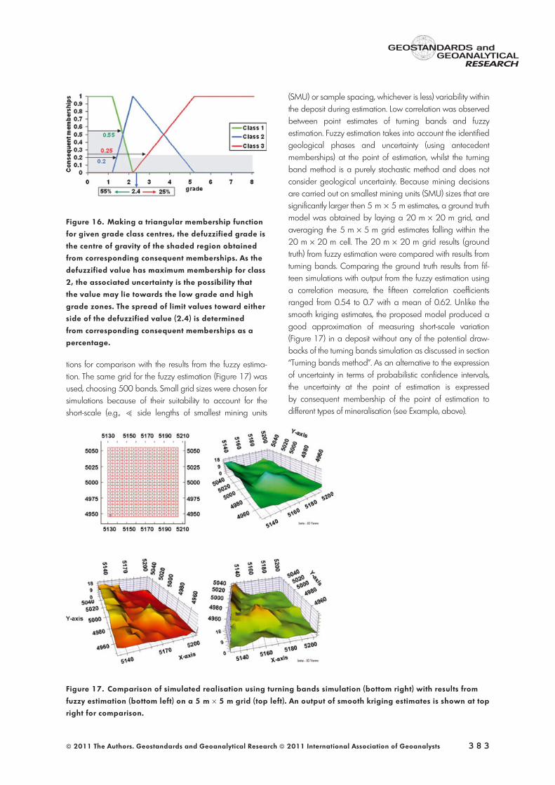
Taking into account the uncertainty associated with thedefuzzified grade, using the consequent memberships, wecan say that there was a 55%, 20% and 25% chance thatthe grade belongs to low, medium and high grade zonesrespectively. As the defuzzified grade lay close to the med-ium grade class centre value, the associated uncertaintywith the defuzzified grade can be expressed such thatthere is 55% chance that the grade may lie towards lowgrade zone and 25% chance that the grade may lietowards high grade zone (see Figure 16). Therefore, it maybe concluded that the grade lies between [2.4-(0.55 · 2.4)] and [2.4 + (0.25 · 2.4)], i.e., between 1.08and 3.0.

Comparison of results from fuzzy estimationwith turning bands simulations

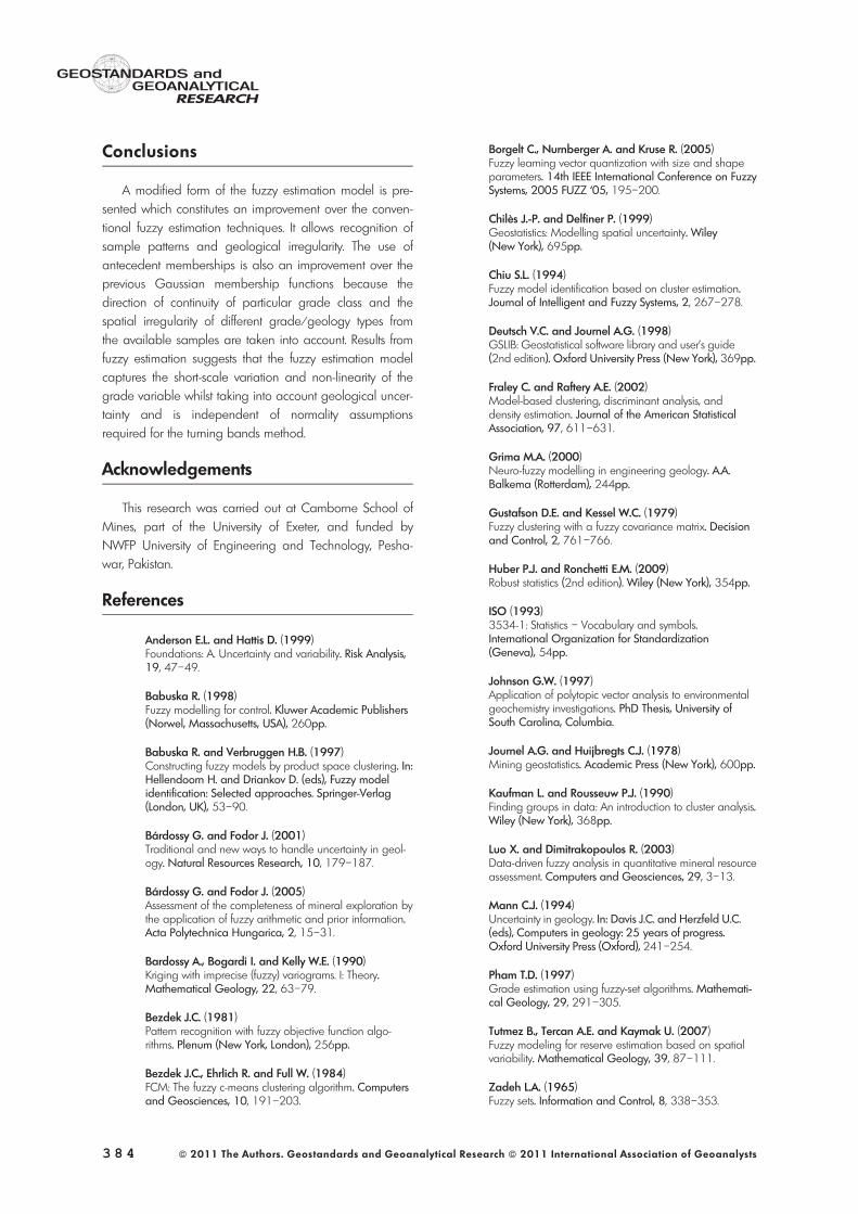
The same technique is followed for all the estimationpoints in the grid. Fuzzy estimation shows non-linear behav-iour of the samples and short-scale variation within thesamples as compared to the simulated estimates at thesame positions in a 5 m · 5 m grid (Figure 17).

The significance of using robust algorithms is a keyaspect in achieving such a prediction model. Similarly, theclassification is then transferred to the point of estimationusing antecedent membership that is independent of aGaussian function and preserves the shape of the grade dis-tribution from the outcome of the classification. The turningbands simulation was carried out to generate fifteen simula-

Table 6.Deriving consequent memberships for point of estimation

Coordinates of known samples Determining the influence of the geology type fromthe known sample class and distance membership

on estimation point (x0, y0)

Productsum

X Y Low grade3 A1

Medium grade3 A2

High grade3 A3

5170 4990 0.67 0.29 0.01 0.975170 4995 0.55 0.39 0.02 0.975165 4990 0 0.02 0.88 0.95165 4995 0.87 0.08 0.02 0.98The total influence of the search neighbourhood on the point of estimation 3.82

Figure 15. Consequent part of the rule, crisp output

values from regression equations and associated con-

sequent memberships at a point of estimation

x0 = 5167.5, y0 = 4992.5 and n0 = 4.


tions for comparison with the results from the fuzzy estima-tion. The same grid for the fuzzy estimation (Figure 17) wasused, choosing 500 bands. Small grid sizes were chosen forsimulations because of their suitability to account for theshort-scale (e.g., > side lengths of smallest mining units

(SMU) or sample spacing, whichever is less) variability withinthe deposit during estimation. Low correlation was observedbetween point estimates of turning bands and fuzzyestimation. Fuzzy estimation takes into account the identifiedgeological phases and uncertainty (using antecedentmemberships) at the point of estimation, whilst the turningband method is a purely stochastic method and does notconsider geological uncertainty. Because mining decisionsare carried out on smallest mining units (SMU) sizes that aresignificantly larger then 5 m · 5 m estimates, a ground truthmodel was obtained by laying a 20 m · 20 m grid, andaveraging the 5 m · 5 m grid estimates falling within the20 m · 20 m cell. The 20 m · 20 m grid results (groundtruth) from fuzzy estimation were compared with results fromturning bands. Comparing the ground truth results from fif-teen simulations with output from the fuzzy estimation usinga correlation measure, the fifteen correlation coefficientsranged from 0.54 to 0.7 with a mean of 0.62. Unlike thesmooth kriging estimates, the proposed model produced agood approximation of measuring short-scale variation(Figure 17) in a deposit without any of the potential draw-backs of the turning bands simulation as discussed in section‘‘Turning bands method’’. As an alternative to the expressionof uncertainty in terms of probabilistic confidence intervals,the uncertainty at the point of estimation is expressedby consequent membership of the point of estimation todifferent types of mineralisation (see Example, above).

Figure 17. Comparison of simulated realisation using turning bands simulation (bottom right) with results from

fuzzy estimation (bottom left) on a 5 m · 5 m grid (top left). An output of smooth kriging estimates is shown at top

right for comparison.

Figure 16. Making a triangular membership function

for given grade class centres, the defuzzified grade is

the centre of gravity of the shaded region obtained

from corresponding consequent memberships. As the

defuzzified value has maximum membership for class

2, the associated uncertainty is the possibility that

the value may lie towards the low grade and high

grade zones. The spread of limit values toward either

side of the defuzzified value (2.4) is determined

from corresponding consequent memberships as a

percentage.


Conclusions

A modified form of the fuzzy estimation model is pre-sented which constitutes an improvement over the conven-tional fuzzy estimation techniques. It allows recognition ofsample patterns and geological irregularity. The use ofantecedent memberships is also an improvement over theprevious Gaussian membership functions because thedirection of continuity of particular grade class and thespatial irregularity of different grade ⁄ geology types fromthe available samples are taken into account. Results fromfuzzy estimation suggests that the fuzzy estimation modelcaptures the short-scale variation and non-linearity of thegrade variable whilst taking into account geological uncer-tainty and is independent of normality assumptionsrequired for the turning bands method.

Acknowledgements

This research was carried out at Camborne School ofMines, part of the University of Exeter, and funded byNWFP University of Engineering and Technology, Pesha-war, Pakistan.

References

Anderson E.L. and Hattis D. (1999)Foundations: A. Uncertainty and variability. Risk Analysis,19, 47–49.

Babuska R. (1998)Fuzzy modelling for control. Kluwer Academic Publishers(Norwel, Massachusetts, USA), 260pp.

Babuska R. and Verbruggen H.B. (1997)Constructing fuzzy models by product space clustering. In:Hellendoorn H. and Driankov D. (eds), Fuzzy modelidentification: Selected approaches. Springer-Verlag(London, UK), 53–90.

Bárdossy G. and Fodor J. (2001)Traditional and new ways to handle uncertainty in geol-ogy. Natural Resources Research, 10, 179–187.

Bárdossy G. and Fodor J. (2005)Assessment of the completeness of mineral exploration bythe application of fuzzy arithmetic and prior information.Acta Polytechnica Hungarica, 2, 15–31.

Bardossy A., Bogardi I. and Kelly W.E. (1990)Kriging with imprecise (fuzzy) variograms. I: Theory.Mathematical Geology, 22, 63–79.

Bezdek J.C. (1981)Pattern recognition with fuzzy objective function algo-rithms. Plenum (New York, London), 256pp.

Bezdek J.C., Ehrlich R. and Full W. (1984)FCM: The fuzzy c-means clustering algorithm. Computersand Geosciences, 10, 191–203.

Borgelt C., Nurnberger A. and Kruse R. (2005)Fuzzy learning vector quantization with size and shapeparameters. 14th IEEE International Conference on FuzzySystems, 2005 FUZZ ‘05, 195–200.

Chilès J.-P. and Delfiner P. (1999)Geostatistics: Modelling spatial uncertainty. Wiley(New York), 695pp.

Chiu S.L. (1994)Fuzzy model identification based on cluster estimation.Journal of Intelligent and Fuzzy Systems, 2, 267–278.

Deutsch V.C. and Journel A.G. (1998)GSLIB: Geostatistical software library and user’s guide(2nd edition). Oxford University Press (New York), 369pp.

Fraley C. and Raftery A.E. (2002)Model-based clustering, discriminant analysis, anddensity estimation. Journal of the American StatisticalAssociation, 97, 611–631.

Grima M.A. (2000)Neuro-fuzzy modelling in engineering geology. A.A.Balkema (Rotterdam), 244pp.

Gustafson D.E. and Kessel W.C. (1979)Fuzzy clustering with a fuzzy covariance matrix. Decisionand Control, 2, 761–766.

Huber P.J. and Ronchetti E.M. (2009)Robust statistics (2nd edition). Wiley (New York), 354pp.

ISO (1993)3534-1: Statistics – Vocabulary and symbols.International Organization for Standardization(Geneva), 54pp.

Johnson G.W. (1997)Application of polytopic vector analysis to environmentalgeochemistry investigations. PhD Thesis, University ofSouth Carolina, Columbia.

Journel A.G. and Huijbregts C.J. (1978)Mining geostatistics. Academic Press (New York), 600pp.

Kaufman L. and Rousseuw P.J. (1990)Finding groups in data: An introduction to cluster analysis.Wiley (New York), 368pp.

Luo X. and Dimitrakopoulos R. (2003)Data-driven fuzzy analysis in quantitative mineral resourceassessment. Computers and Geosciences, 29, 3–13.

Mann C.J. (1994)Uncertainty in geology. In: Davis J.C. and Herzfeld U.C.(eds), Computers in geology: 25 years of progress.Oxford University Press (Oxford), 241–254.

Pham T.D. (1997)Grade estimation using fuzzy-set algorithms. Mathemati-cal Geology, 29, 291–305.

Tutmez B., Tercan A.E. and Kaymak U. (2007)Fuzzy modeling for reserve estimation based on spatialvariability. Mathematical Geology, 39, 87–111.

Zadeh L.A. (1965)Fuzzy sets. Information and Control, 8, 338–353.


Appendix A

List of symbols

2 Predefined termination measure for the GK algorithml0i Consequent memberships for the ith class at point of estimation (x0, y0)ari The effect of ith class from rth known sample within the search neighbourhood on the point of estimationai Consequent memberships of the ith class(x0, y0) Any point of estimation defined in the input spaceAi ith class Mahalanobis distance based membership of the known sample to the point of estimationai0 Constant term of regression parameters for the ith classai1 ….. aip p-dimensional input space regression parameters for the ith classc Number of mineralogical phases ⁄ grade classesd0i Mahalanobis distance in the input space between point of estimation and the ith class centredij Distance of the jth sample from the ith class centredir Class-specific (ith class) Mahalanobis distance in input space between rth known sample within the search neighbourhood and

a point of estimationFi Input part (first p · p part) of fuzzy covariance matrix for the ith classg N · 1 column vector with known grades of N samplesgi (x0, y0) Grade output from the ith rule for a point of estimationgj Grade output variable of jth known sampleJ Objective functionj Sample numberk kth line in turning bandsL Number of lines in turning bandm Fuzziness indexN Number of samplesn0 The number of known samples in search neighbourhood used for estimating any point defined by (x0, y0) in two-dimensional

input spacep Dimensions of the input spaceP Total number of data dimensionsPi Regression parameters vector for the ith classSi Volume reduced fuzzy covariance matrix for the ith classSi

* Fuzzy covariance matrix for the ith classt Iteration numberuij Membership of jth sample to the ith class centreuri Membership of the rth known sample in the search neighbourhood to the ith classWi N · N matrixX Data matrix with all variables (columns) and samples (row)X X-axisY Y-axisx0 p-dimensional vector of the point of estimation in the input spaceXe (N · p + 1) matrixxj jth sample vector with all input and output variablesxj1….. xjp Input variable components of jth samplexr p-dimensional vector of the rth known sample used in estimation of x0

zk(x0, y0) Non-conditional simulated value at point of estimation on kth line


modelling short-scale variability and uncertainty during mineral resource estimation using a novel...

Documents