modelling seismic hazard for mines -...

Modelling Seismic Hazard for Mines

Aleksander J. Mendecki & Ernest C. LötterInstitute of Mine Seismology, Australia

Australian Earthquake Engineering Society 2011 Conference18-20 November Barossa Valley, South Australia

AbstractUnlike earthquakes, seismic rock mass response to mining can be controlled.

Seismic hazard in mines is driven by the volume and the spatial and temporaldistribution of rock extraction. To forecast seismic hazard for a given minelayout we need to extrapolate its parameters in the volume mined domainrather than in time.

It is difficult to reconcile the far-field point source model and groundmotion recorded away from seismic sources, where details of the ruptureprocess are hidden, with the violent nature of damage resulting from majorrockbursts. From linear elastic considerations the rate of stress release withan increase in slip velocity must, at all times, be less than the acousticimpedance, ρvS . The maximum possible ground velocity is then limited bythe bulk shear strength of the rock, σbss, and may be roughly estimatedas umax = 0.5 σbss/ρvS . However if the rate of loading exceeds the rate atwhich energy can be removed by elastic waves the large strains may have totravel faster than small ones generating extreme ground motion that extendsfurther away from the source.

Seismic networks in mines are not suitable to measure strong groundmotion close to excavations. Therefore to assess damage potential to mineinfrastructure one needs to model ground motion produced by large seismicevents expected in a given area. Preliminary results of 3D finite-differencekinematic modelling applied to complex source mechanisms in the presenceof underground excavations are presented. This includes two-fault systemsproposed by Ortlepp, 1984 and 1997, as well as simulations of surface groundmotions in an urban environment. A rotated staggered grid is used as basisfor the forward model, which simplifies the implementation of free surfaceconditions and is more applicable to the highly heterogeneous medium modelin mining situations. Even when the static source parameters are kept fixed,there are great differences in resolved ground motions at points of interestunder different rupture velocities and slip distributions.

1 Earthquakes vs Mining Induced Hazard

Earthquake driving forces can not be controlled. They are fairly constant andrelatively slow compared to changes in stresses induced by mining. This slowloading facilitates the process of self-organisation that leads to a state at which

Mendecki and Lötter: Modelling Seismic Hazard for Mines 2

the system develops reproducible relationships among its distant parts (Nicolisand Prigogine 1989; Rundle et al. 2002). It is assumed that this growth oflong range correlations allows for progressively larger events to be generated.These large events in turn partially de-correlate the system and the processcontinues (Sornette, 2005). In such a case having a sufficiently long catalog of pastearthquakes and realistic data on geological structures would give a reasonableindication of future hazard. But the time scales involved here are huge andseismological data is far from adequate. The causative faults are inaccessibleand the inferred information about their extent, orientation and properties issparse.

For systems driven steadily over long periods of time the sequence of recordbreaking events is a monotonously increasing function of time with decreasinggradient (e.g. Chandler, 1952; Glick, 1978; Mendecki, 2008; Van Aalsburg et al.,2010). Therefore the problem of estimating the maximum possible magnitude ofan earthquake in a given area, mmax, may be reduced to finding the truncationpoint of the observed distribution of past events. An obvious estimator here ismmaxo - the largest observed event, which will underestimate mmax, but the biasshould decrease as the size of the data set increases. After correction for thebias (Robson and Whitlock, 1964; Cooke, 1979; Kijko, 2004) the estimated mmax

is a fraction greater than mmaxo. The exponents of the observed power law sizedistribution of global and regional seismicity are remarkably stable (Wesnousky1999).

20-Dec 25-Dec 30-Dec 04-Jan 09-Jan0

1500

3000

4500

6000

Vm

[m

3]

Vm

0

1000

2000

3000

4000

5000

Cum

ula

tive

Act

ivit

y

Activity

Figure 1: Drop in the rates of seismicactivity during 2010 Christmas break ina gold mine in South Africa.

Mining is not a spontaneous process.It induces stresses at a particularplace, at a particular time and at aparticular rate which are all highlyvariable compared to the tectonicregime. An average rate of deformationinduced by mining is at least twoorders of magnitude greater thanthe average slip rate of tectonicplates. The instantaneous closureafter production blasts of tabular reefsin a deep South African gold mine canbe as high as 1 cm, followed by asteady state closure at the rate of 1.5cm/day for a number of days (Malan,

1999). Underground openings facilitate deformation and relaxation of stresses,hence aftershock sequences, even after larger events in mines, continue only forfew days - not for years.

Given some short time delay for rock mass excitation and relaxation, thebulk of seismic activity in mines starts with rock extraction, increases with theextraction ratio of the ore body and stops with cessation of mining. Figure 1presents an example of seismic rock mass response to the 11 days productionbreak over December and January 2010. Large scale mining taking place over

Australian Earthquake Engineering Society 2011 Conference, Barossa Valley


number of years, however, alters the regional stress regime and may induceearthquake type events which are less correlated with the recent mining, e.g.Belchatow m4.6 in 1980 (Gibowicz et al., 1981), Newcastle m5.6 in 1989 (Gibsonet al., 1990; Klose, 2007), Kalgoorlie m5.1 in 2010 (Hao, 2010; Cranswick, 2011),Welkom m5.0 in 1976 (Van Aswegen, 1990; Ortlepp, 1997) and Klerksdorp m5.3in 2005 (Durrheim et al., 2006).

Seismic events in mines can be considered as small earthquakes, thereforetheir magnitude should scale with energy, E, and potency - the product of anaverage slip and source area - P = uA, as m∝ logE ∝ logP , as oppose to moderateto large earthquakes where scaling is m ∝ 2/3logE ∝ 2/3logP (Kanamori andAnderson, 1975; Mendecki, 1993 Figure 1.2; Ben-Zion and Zhu 2002). Miningdistricts are not well covered by the national seismological networks and it isdifficult to calibrate their magnitude scales. Since the accuracy of magnitudedetermination in mines is 0.25 to 0.5 unit, one can use the relevant moment orpotency-magnitude scale, e.g. m = logP + 0.32, given by Gibowicz (1975), orsimply use logP as a measure of magnitude.

The catalogue of mine seismic data in most cases is adequate and the geologyof the ore body and the surrounding rock mass is well explored. Past data isuseful to compare seismic rock mass response to different mining scenarios but,because of the intermittent nature of loading, is not the best indication of futurehazard. To forecast future hazard we need to take into account future mining(Mendecki, 2008).

Mon Tue Wed Thu Fri Sat Sun0

5000

10000

15000

20000

25000

30000

Nu

mb

er

of

Ev

en

ts

Figure 2: Day of week distribution of seismic activity over 3 years in a minewith limited production on Saturdays and no production on Sundays (left).Potency-frequency plot over the same period of time with recurrent volume mined(right).

Figure 2 (left) shows day of week distribution of seismic activity over 3 yearsin a mine with limited blasting on Saturdays and no production on Sundays andFigure 2 (right) shows the potency-frequency distribution of the same data set.Note that the recurrence time at Figure 2 (right) has been replaced by the averagevolume mined to produce an event above a certain size. The mean inter eventtime for events with logP ≥ 0.5 is 2.96 days with a standard deviation of 4.54



days. This gives a coefficient of variation, Cv = 4.54/2.96 = 1.53. The mean interevent volume mined Vm is 655 m3 with a standard deviation of 298.76 m3, whichgives Cv = 0.45. The higher the coefficient of variation the more variable, orclustered, is the process. The uniform distribution has zero standard deviationtherefore Cv = 0, a quasi-periodicity is characterized by 0 < Cv < 1 and clusteringby Cv > 1. It is therefore more informative to quote an average volume to bemined to produce a given seismic activity rather than the recurrence time. Largeevents in mines tend to be more randomly distributed and both the volume minedand recurrence time have a similar distribution.

Ground motion in mines is recorded only at a limited number of sites andfrequently far from active excavations where instrumentation is difficult. Mostsystems in mines do not measure ground motion at the skin of excavations. Theyare designed to locate events and to estimate their source parameters. For thisreason seismic sensors are placed in boreholes, away from excavations, to avoidthe very site effects that amplify ground motion. As a result seismic hazardanalysis in mines is limited to estimates of probabilities of occurrence of seismicevents above a certain magnitude.

The probability that an event will exceed potency P while mining the volumeof rock V∆m over time ∆T into the future can be given as

Pr [≥ P, V∆m] = 1−(

1

1 + Pr (> P,α(V∆m), β(V∆m))

)n[α(V∆m),β(V∆m)]+1

, (1)

where n[α(V∆m), β(V∆m)] is the expected number of events above the thresholdmagnitude Pmin, the V∆m and Pr (> P,α(V∆m), β(V∆m)) is the expected survivalfunction of the assumed potency-frequency distribution with parameters α, thatmeasures the activity rate, and β which is the exponent, both functions of thevolume already mined and to be mined. Equation (1) takes into account theinherent uncertainty in the rate of occurrence of seismic events (Benjamin, 1968;McGuire, 1977; Campbell, 1982).

The most frequently used survival functions to estimate seismic hazard are:(1) the open-ended power law with no limit on maximum event size, (2) theupper-truncated power law with hard limit Pmax and (3) the Gamma-type whichis the product of the open-ended survival function and an exponential taper whichconstitute a soft limit Pmax, above which the probability decays quickly but isfinite. The sequence of the record highs in mines is jerky, therefore for short termhazard it is more useful to define Pmax+1 - the next record breaking event, asopposed to the largest ever possible. The correcting term here can be logPmax+1 =logPmaxo + max (∆ logPmaxo), where the max (∆ logPmaxo) is the maximum jumpin the logarithms of the observed series of record potencies (Mendecki, 2008).Since mining scenarios may change, it is advisable to select the past data thatis most relevant to future mining. In mines α tends to increase and β tendsto decrease as extraction ratio increases - therefore they are functions of thevolume mined Vm. By extrapolating the observed relationship between α, β andthe volume mined, or time, see dotted lines in Figure 3, we can forecast futurehazard for different production scenarios using equation (1).



0 2000 4000 6000 8000 10000 12000

Vmeff

0

50

100

150

200

250

300

350

400α

0.6

0.64

0.68

0.72

0.76

0.8

0.84

β

Figure 3: Parameters α (triangles) andβ (circles) versus volume mined for twoSouth African mines.

All else being equal, seismic hazard inmines is driven mainly by volume andthe spatial and temporal distributionof rock extraction. In general, miningscenarios that induce spatial andtemporal heterogeneity, or disorder,tend to de-correlate the system andare less likely to generate largerdynamic instabilities (Mendecki, 2005).Therefore, unlike earthquakes, seismichazard in mines can largely becontrolled. Introducing stabilisingpillars, backfill, changing the sequenceof mining or reducing the extractionratio may all mitigate seismic response

(e.g. van Aswegen and Mendecki, 1999; Handley et al., 2000; Capes, 2010).

2 Near-Source Ground Motion

Figure 4: Peak accelerations of 53 m/s2

at 1550 Hz (u = 5.6·10−7m) recorded 108m from logP = -1.3 event at Ridgewaymine. The sampling rate is 6 kHz, theresonance frequency of the sensor is 15kHz and the response of its internalfilter drops to -3 dB at 2.3 kHz whichmarks the upper limit of the usablefrequency band.

The maximum ground motions thatcan be experienced at a site close tosource are controlled by the maximumslip velocity, the interaction of radiationfrom different parts of the sourceand from different travel paths, andby the site effects. Severe damageto underground excavations in minesis observed mainly near the sourcearea. Minor damage can be causedby ground velocities as low as fewcm/s. Falls of ground in poorlysupported areas can be triggered byground motion as low as a fewmm/s. There is a weak correlationbetween damage and the observedpeak acceleration. Small eventsmay generate large accelerations butat high frequencies, therefore theyproduce little deformation, u ∝ u/f2 ,

see Figure 4.The ground velocity at source is controlled by the maximum stress at source

which, in turn, is limited by the strength of the rock mass. Consider a small pieceof ground attached to an infinite source bounded across a plane by the extent of arupture propagating with velocity vr over small increment of time ∆t, and awayfrom the source plane by the extent of the propagating S-wave with velocity vS ,



see Figure 5. If the applied effective stress σeff available to accelerate the twosides of the source is released instantaneously then the rock mass acceleration,u, and velocity, u, can be derived from u = F/m, where here force F = σeff (vr∆t)

2

and mass m = ρ(vr∆t)2vS∆t, therefore

u =F

m=

σeffρvS∆t

=σeffµ∆t

vS ; =⇒ u =F∆t

m=σeffρvS

=σeffµ

vS , (2)

where µ = ρv2S is rigidity and ρvS is the shear wave impedance.

Figure 5: Sketch of a volume of groundattached to a moving fault.

According to the above equations:(1) Rock strength does not limitpeak acceleration. For small ∆t(at high frequencies, 1/∆t) there ispractically no limit on peak groundacceleration. Fracture in a continuummay produce a steep change in velocitywhich results in high accelerationat high frequencies (Andrews et al.,2007). (2) The ground velocity willalways be much smaller than therupture velocity because the effectivestress is much smaller than the shearmodulus. (3) Rock strength limitsground velocity, which does not dependon frequency. (4) Ground velocity at

source does not depend on magnitude.For a finite source of size 2r with instantaneous stress release the effects of

the edges of the crack will abate the ground velocity with time. For a simpletaper, exp (vSt/r), given by Brune (1970), integration of equation (2) over processtime, r/vS , gives the average ground velocity 〈u〉 = 0.63 σeffvS /µ (Kanamori, 1972).The near source ground velocity for a finite source and finite rupture velocity fordifferent source models are quoted in Table 1.

Table 1: Models of near-source ground velocity as a function of rupture velocity

Model/Author 〈u〉 for vr = 0.75vSBilateral rupture(Burridge, 1969)

〈u〉 = σeff/ [ρvS (1 + vS/vr)] 〈u〉 = 0.43σeff/ρvS

Dynamic cohesive rupture(Ida, 1973)

〈u〉 = σeffvr/(ρv2S

)〈u〉 = 0.75σeff/ρvS

Dynamic rupture scaling(McGarr and Fletcher,

2001)〈u〉 = 0.8σeff/ [ρvSf (vr)] 〈u〉 = 0.36σeff/ρvS

The effective stress cannot be measured directly but different approximationscan be made. One option is to assume that σeff is equal to the bulk shear



strength of the rock within the volume of interest, which for most hard rocksvaries between 40 and 80 MPa. An intact rock may be considerably stronger. If areliable data base is available one can also use the maximum stress drop derivedfrom recorded waveforms, which in South African gold mines varies between 30and 60 MPa. According to equations quoted in Table 1 for σeff = 50 MPa, µ =30 GPa, vS = 3300 m/s and vr = 0.75 vS the estimates of the near source groundmotion would vary between 2.0 m/s and 4.0 m/s.

An average ground velocity at source can also be estimated from 〈u〉 = u/(2τ),where u can either be observed in the field or estimated from the scaling relation,e.g. u = 0.00225 3

√P (Somerville et al., 1999), and τ is the rise time taken from the

recorded waveforms. The division by a factor of 2 comes from the fact that thenear-source ground velocity is equal to half of the slip velocity vslip - the velocityof one side of the source with respect to the other.

In mine seismology the issue of the maximum possible ground motion withinthe source volume is debatable. Extreme damage experienced during shear-typeevents cutting through pristine rock where no discernible planar weaknessesexisted before implies ground motions well above the accepted 3 m/s limit (seeOrtlepp, 1984, 1997, 2006). During such events the surrounding rock is shatteredinto small fragments and pulverized, with particles less than 25 µm in size, andhydraulic props punched deep into the quartzite foot-wall (Ortlepp et al., 2005;see also Sammis and Ben-Zion, 2008; Yuan et al., 2011). These events mightimpart extreme ground motions in the form of localised, directional and focusedshock waves into the surrounding rock, as illustrated in Figure 6.

Figure 6: Mechanism for creatingextreme compressions and rarefactionsalong a non-smooth fault surface andgenerating localised, focused strongground motions (Ortlepp et al., 2005).

Equations (2) and in Table (1) areapplicable when the rate of stressrelease with an increase in slipvelocity is, at all times, less thanthe shear wave impedance, dσeff/dv< ρvS . Slip rates given by theseequations may underestimate strainrates at the edges of the movingsource. If the rate of loading exceedsthe rate at which energy can beremoved by elastic waves the systemis no longer linear. To remove thisexcess energy the large strains needsto travel faster than small ones -the particle velocity exceeds the shockwave velocity (Knopoff and Chen,2000). This is also what happens

during super-shear rupture when the crack tip is moving faster than the S-wavevelocity (e.g. Weertman, 1969; Burridge, 1973; Savage, 1971; Andrews, 1976;Olson and Apsel, 1982; Archuleta, 1984; Spudich and Cranswick, 1984; Dunham,2007; Lu et al., 2010).



3 Modelling Ground Motion in Mines

Modelling of ground motions in an elastic medium is governed by the equationsof motion, i.e. the momentum conservation equations and stress-strain relations

ρu = ∇ · σ + f ; σij = cijklεkl (3)

where the elasticity tensor cijkl can be parametrised for isotropic media by thetwo Lamé parameters λ and µ. This parametrisation leads to the equation

σ = λ∇ · uI + µ(∇u + (∇u)T ) (4)

While analytical solutions exist for homogeneous medium (constant densityρ and material parameters λ and µ), to model a heterogeneous mine model thatmay contain free surfaces, caves, stopes and other material contrasts, a numericalsolution is needed.

Figure 7: Elementary (2D) cell forvelocities and stresses in rotatedstaggered grid scheme.

A numerical solution of the 3Dwave equation is achieved by finitedifference modelling. As a first step,partial derivatives in Equation 3 arereplaced by numerical first, secondor fourth order estimates obtained bya Taylor expansion truncated afterthe desired number of terms. Thedecision on where on a finite differencegrid to place spatially dependentmaterial properties (ρ,λ and µ) andphysical quantities (vi, σij) constitutea choice between various staggeredgrid schemes. A fourth-order in spacescheme is described in Graves (1996).

Another scheme is introduced bySaenger and Bohlen (2004) which represents the finite difference grid as a rotatedgrid (Figure 7), with the advantage that all material properties and physicalquantities are placed within one elementary grid cell from point values beingupdated. This allows for the accurate modelling of elastic waves traversingmaterial contrasts, cracks or free surfaces without the need to explicitlyimplement boundary conditions.

Performing forward modelling of a seismic source using the finite differencemethod thus firstly requires an accurate description of the elastic medium, whichis done by assigning values to the density ρ and material parameters λ and µ ateach grid point. Moreover, absorbing boundary conditions on the model domainneeds to be added, either by following the A1 absorbing boundary condition ofClayton and Engquist (1977) that assumes planar waves, or an attenuating shellaround the model that simulates inelastic attenuation. It reduces the influenceof non-physical wave reflections off the side of the finite difference model.



Figure 8: An extended source built froma distribution of point sources.

Inserting one or multiple pointsources into a model is convenientlydone by applying time dependent bodyforces using the last term of Equation(3 ). These force representations isconvenient in the staggered grid ofsimple moment sources with arbitrarymechanisms (Graves, 1996).

Modelling a finite source on afinite difference grid is done bysuperposition of the wave fields fromby multiple point sources. These pointsources represent point-like parts ofthe extended source. The seismic

potency of the finite source is the sum of the potencies of the constituent pointsources, and it is expected that these point sources will have similar principalaxes, but may vary in magnitude, as not all parts of the source will experiencethe same net displacement.

Figure 8 demonstrate such a simple scheme with colours proportional to thefinal displacement experienced by each point. At the edge of this elliptical source,displacement tends towards zero (blue), while maximum displacement occurs atan off-center point on the principal axis of the source ellipse.

When building a kinematic model of an extended source, the consistency ofthis set of source parameters and time histories for each point of the fracturingfault is very important. Two features of seismic sources that enforce strongconstraints on the possible distributions of these parameters are self-similarity ofthe final slip distribution and the expected characteristics of the high frequencypart of the displacement spectrum as seen in the far field. These consistencyconstraints on a set of point sources must ensure smooth and monotone sliphistories for all parts of the source, while staying physically reasonable.

To provide explicit constraints on the parameters controlling the rupture, thekinematic k-square earthquake source model of Herrero and Bernard (1994) canbe used. This model yields ω−2 far field radiation and k−2 slip distribution,meaning that spectral amplitudes of the final slip distribution decay as a powerof 2. The idea is, instead of describing the distribution of slip on a fault, ratherto describe its Fourier transform. Then the same type of Fourier transformproduces similar slip distributions for faults with different dimensions. Thek-square model thus represents final displacement at (x, y) on the fault as

u(x, y) =

ˆ ˆD(kx, ky)e

i(xkx+yky)dkxdky (5)

where D (kx, ky) = exp [iΦ (kx, ky)] /

√1 +

[(kx/kc)

2 + (ky/kc)2]2

, with the functionΦ(kx, ky) in the Fourier transform being a random phase. For large values ofthe wave-number, the Fourier transform decays as the inverse of the square. An



extended source is then constructed by distributing its total seismic potency overthe sub-sources, proportional to the modelled permanent displacement at theirpositions from the k-square model. For sub-source i, we thus obtain P i0 = ui4Awith the areas of all sub-sources the same due to the constant gridding. Similarly,rise times over different parts of the source are chosen to be proportional to thefinal slip, thus Ti = Tmax u(ξi,ηi)

umaxwhere Tmax is a chosen rise time corresponding

to the sub-source with maximum final displacement.The slip velocity time-function of a sub-source determines the high frequency

behaviour of the amplitude spectrum in the far field. Beresnev and Atkinson(1997) have proposed a simple model of a slip velocity time function which leadsto a far field displacement spectrum adhering to ω−2 decay. The parametrisationof the source time function ν (t; τ, ζ) ' t exp (−2t/τ) allows us to model our chosenrise time for the extended source by choosing τ = 1

2Tmax.

To choose initiation times ti0 for sub-sources, consider that these must coincidewith the time when the rupture front reaches the location of the sub-source. Arupture propagation model thus needs to be imposed in order to determine theinitiation times for all sub-sources and hence complete the kinematic model ofthe extended source. If the simple assumption is made that rupture speed isfaster when parallel to slip and slower when orthogonal to slip, we obtain anextended source in the shape of an ellipse, with eccentricity determined by theratio of these two orthogonal rupture velocities. This is the scenario illustratedby Figure 8.

The initiation times can be calculated by integrating the rupture propagationvelocity along the line that connects the sub-source with the hypocenter. Now,the ground motion experienced at a site is controlled by the maximum velocity ofdeformation at the seismic source (slip velocity), by the interaction of radiationfrom different sub-sources from different travel paths and by site effects.

3.1 Extended sources in heterogeneous media

Displacement on a fault originates at the focus, and propagates towards its edges.As the focus is not necessarily in the center of the fault, much of the propagationis unidirectional. To examine the extreme ground motions that can be caused atpoints of interest specifically in the direction of rupture propagation, we modelledtwo similar extended sources based on the same k-square slip distribution, butwith distinct rupture mechanisms. These rupture mechanisms are: vr = 0.9vS forsub-shear rupture process and vr =

√2vS for super-shear process where rupture

propagates faster than S-wave velocity. Also present in this model is a tabularstope that causes reflections and partly obstructs waves from directly travellingto the upper part of the rock mass.

Snapshots of the seismic wave field are shown in Figure 9 and 10. FromFigures 9 and 10 (for which corresponding frames refer to the same points intime), it is clear from inspection of the wave field that rupture progresses fasterin the super-shear case and that a Mach cone evolves (see Figure 10 frame 4).



Figure 9: Snapshots in section view of subsequent time steps in a sub-shearrupture process, chronologically from left to right, top to bottom.

Figure 10: Snapshots in section view of subsequent time steps in a super-shearrupture process, chronologically from left to right, top to bottom.

3.2 Complex sources in heterogeneous media : Ortlepp source

Figure 11: Strike section througha stope showing a double sourcemechanism conceptualised by Ortlepp,1984 and Ortlepp, 1997.

We model a complex source modelconceptualised by David Ortlepp anddescribed in Ortlepp (1984) and Ortlepp(1997) page 63 caption (e), see Figure11. It is a superposition of tworectangular extended faults, each ofwhich is similar to the single faultsources described in the previoussection. The first fault is further awayfrom the stope and it induces ruptureon the secondary fault that interactswith the stope. Here we assume thatthe second rupture is induced by thefirst one almost immediately.

Due to the freedom availableto place sub-sources on the finite

difference grid, we are now able to independently choose both the orientationsof these faults and the velocity of rupture propagation, vr. In particular, this



allows modelling of the first (initiating) fault to have sub-shear rupture velocity(vr < vS) and the second (primary) fault to have super-shear rupture velocity(vr > vS). In Figure 12 the rupture and slip histories of such a scenario areillustrated, demonstrating that at given points on the fault, rupture direction andslip direction need not be the same. For our model, we introduce a fault with a dipof 60◦, touching a horizontal stope. Some points of interest are marked around it,to represent points where we will compute ground motions. In particular, as therupture mechanism of the fault will be starting below and progressing upwards,we are especially interested in comparing ground motions of the footwall and thehanging wall. This is illustrated in Figure 12.

(a) Rupture history of theOrtlepp source, with initiationtime per point obtained fromradial distance from the focus.

(b) Slip history of theOrtlepp source, with finaldisplacements determined bya k-square distribution.

(c) Synthetic sensor placementaround the fault-stope corner.

Figure 12: Comparison of rupture (a) and slip (b) histories for the Ortlepp source.The horizontal structure is a thin tabular stope that can be chosen to intersectthe secondary fault. Sensors 4, 7, 9, 11, 12 and 15 (c).

0 0.2 0.4Time [s]

-3

-2

-1

0

1

2

Ve

locity [

m/s

]

VxVy

Vz

Velocity components near the fault-footwall corner

(a) Sensor 4: Velocities nearfault and footwall corner

0 0.2 0.4Time [s]

-4

-3

-2

-1

0

1

2

Ve

locity [

m/s

]

VxVy

Vz

Velocity components just ahead of the stope

(b) Sensor 7: Velocities justahead of the stope

0.1 0.2 0.3 0.4Time [s]

-10

-5

0

5

Ve

locity [

m/s

]

VxVy

Vz

Velocity components close to the fault

(c) Sensor 9: Velocities closeto the fault.

Figure 13: Synthetic seismograms recorded around the fault.

After performing the kinematic model run, we investigate the recorded velocityseismograms at sensors 4, 7 and 9 (Figure 13 (a)-(c)). This shows particle velocitiesclose to the fault exceeding 10 m/s at Sensor 9. Both points of interest at Sensors4 and 7 (which are opposing each other in respectively the footwall and hanging



wall of the fault) experience about 2 m/s velocities, although higher frequencycontent is observed at Sensor 7 due to interaction of the stope with the wavefield.

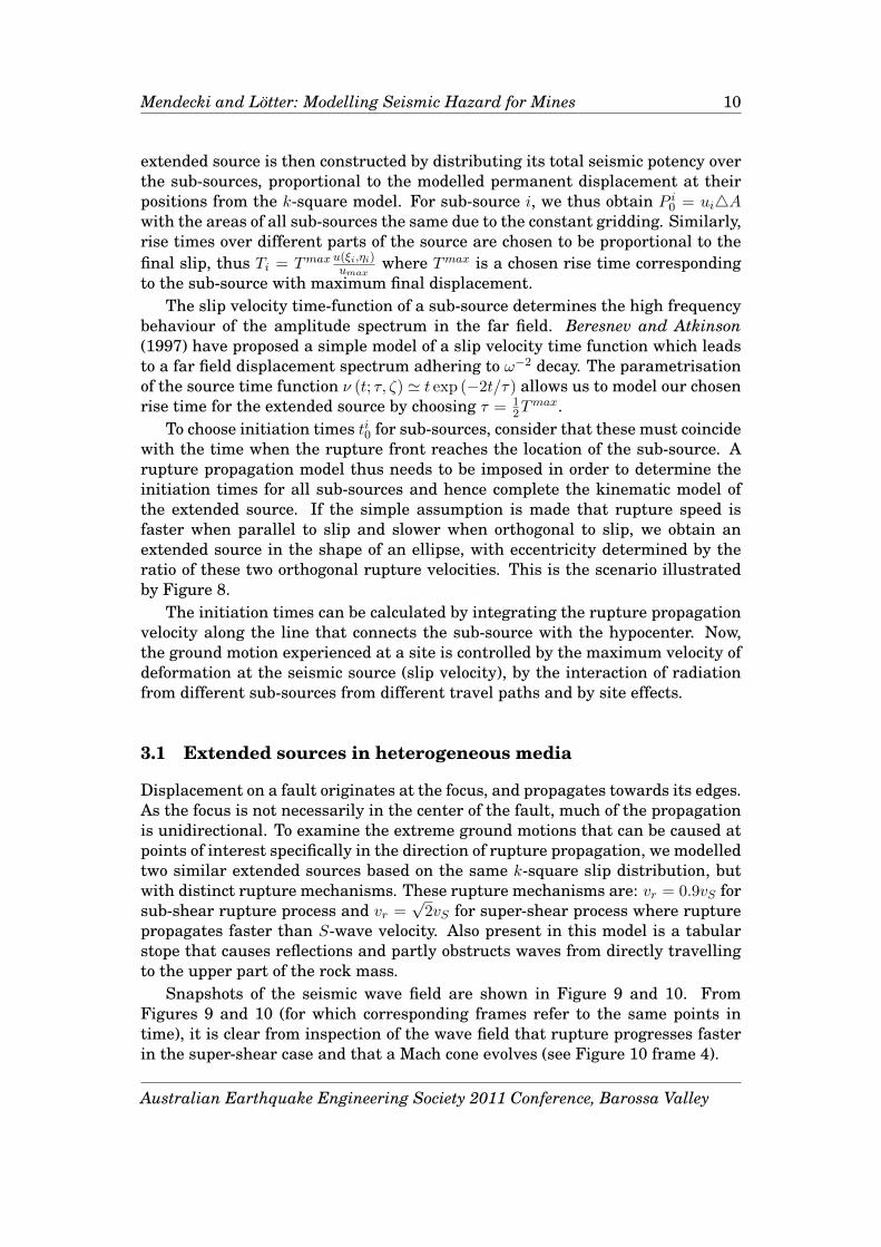
Figure (14) compares the synthetics of Sensor 12 (hanging wall) that is justabove the stope, with that of Sensor 15 (footwall) that is just below the stope.

0 0.2 0.4 0.6 0.8 1Time [s]

0

0.5

1

1.5

2

2.5

Velo

city [m

/s]

Footwall sensorHangingwall sensor

Ground velocity ||V(t)|| below and above the stopeComparison of Sensor 12 and Sensor 15

Figure 14: Synthetic seismograms(as absolute velocity) comparing thehanging wall and footwall groundmotions of Sensor 12 and 15.

Clearly the footwall sensor recordsground motion before the hanging wallsensor due to the shorter distanceto source, but additionally as elasticwaves need to pass around the stope(modelled as air), the later arrivalsat the hanging wall have significantlylower amplitudes. This effect wouldnot have been accurately estimatedusing routine quick estimates of PGVfrom ground motion relations that donot take the real material propertiesof the mine excavation into account.

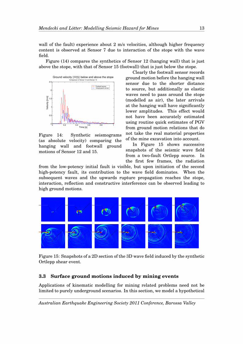
In Figure 15 shows successivesnapshots of the seismic wave fieldfrom a two-fault Ortlepp source. Inthe first few frames, the radiation

from the low-potency initial fault is visible, but upon initiation of the secondhigh-potency fault, its contribution to the wave field dominates. When thesubsequent waves and the upwards rupture propagation reaches the stope,interaction, reflection and constructive interference can be observed leading tohigh ground motions.

Figure 15: Snapshots of a 2D section of the 3D wave field induced by the syntheticOrtlepp shear event.

3.3 Surface ground motions induced by mining events

Applications of kinematic modelling for mining related problems need not belimited to purely underground scenarios. In this section, we model a hypothetical



event that is induced by rising groundwater in abandoned mines close to a majorcity.

N S

JHB CBD

EPICENTER

HYPOCENTER

Granite

Quartzite

1 2

3

Figure 16: Points of interest at whichseismograms are recorded. Sensor 1 isjust below the urban area of interest,Sensor 2 at epicenter and Sensor 3 ishalfway between the hypocenter andurban city center.

In our model, we choose theevent to be 1.5 km below surface,epicentrally 5 km from the major citycentre. The event is modelled as a300 m x 100 m finite elliptical reversefault with a strike of 0◦, dip of 45◦ andrake of 90◦. Maximum slip velocity ischosen to be 2 m/s and the averagedisplacement over the whole sourceu = 0.2 m. We assumed logP = 3.5and a predominant frequency of 3 Hz.

The model domain is assumedmostly homogeneous with a soil layerof three grid points (spacing of 25m) atthe free surface. For the hard rock wechoose ρ = 2700 kg/m3, VP = 5500 m/sand VS = 3500 m/s whereas for the 50m soil layer (which is constructed over

the top three grid points in the rock below the air in the finite difference grid)we choose ρ = 2000 kg/m3, VP = 4000 m/s and VS = 2000 m/s. To model the freesurface effect and air above it, we choose ρ = 2000 kg/m3, VP = 300 m/s and VS = 0m/s with high density to avoid stability problems during the kinematic modellingphase on the finite difference grid.

Figure 17: Snapshots of velocity fields during subsequent stages of the kinematicmodel run of underground event and observed surface ground motions. Theintersection of the two vertical sections represents our point of interest, the areabelow the urban area where damage could potentially occur.

We have computed waveforms in three points of interest indicated at Figure16. Forward modelling allows us to track velocities and dynamic stresses of thewave field not only at the points of interest, but in the entire model domain. Thuswe can simultaneously represent these velocities on multiple planes of interestin subsequent time snapshots. This representation is shown in Figure 17:

With reference to Figure 16, we have recorded synthetic seismograms at Sensors1-3, and these are shown in Figures 18a, 18b and 18c. For each of these, weshow only the vertical component (blue) and the horizontal component (green)



due to our synthetic source being symmetrically aligned in the plane formed bythe sensors.

0 1 2 3 4

Time [s]

-0.02

-0.01

0

0.01

0.02

Gro

un

d M

otio

n [

m/s

]

Ground motion at surface in center of hypothetical city

(a) Unfiltered syntheticseismogram at Sensor 1.At surface in the area ofinterest, both horizontaland vertical ground motionsexceeding 15 mm/s areobserved, at an observedpredominant frequency of 5.8Hz.

0 1 2 3 4

Time [s]

-0.04

-0.03

-0.02

-0.01

0

0.01

0.02

0.03

0.04

Velo

city [m

/s]

Ground motion at epicenter

(b) Unfiltered syntheticseismogram at Sensor 2.Significant vertical groundmotion is observed, resultingin (after integrating todisplacement) permanentdisplacement of over 1 mm.

0 1 2 3 4

Time [s]

-0.02

-0.015

-0.01

-0.005

0

0.005

0.01

0.015

0.02

Gro

un

d M

otio

n [

m/s

]

Ground motion at halfway markPoint halfway between hypocenter and surface point of interest

(c) Unfiltered syntheticseismogram at Sensor 3.Here the initial arrivalsand their immediate codaare clear of reflected waves,as this synthetic recordingis underground, halfwaybetween the hypocenter andpoint of interest on surface.

Figure 18: Synthetics at three points in the simulation of ground motions nearsurface. The predominant frequency at Sensor 1 was calculated by computing apower spectrum over the two non-trivial components of the observed waveform.The energy of the ripple observed at Sensor 2 at around 2s is 10 Hz (taken asaverage over 8 consecutive full periods). While potentially a numerical effectthis can be compared to the expected horizontal S wave resonance (20 Hz) andexpected vertical S wave resonance (10 Hz).

At Sensor 2 (Figure 18b) significant vertical ground motions are observed, butare not expected to be particularly damaging to surface structures. By virtue ofthe displacement curve obtained by integrating this velocity time series, there isclearly an upwards permanent displacement of the surface at this sensor, whichcorresponds with what is to be expected of reverse faulting (Figure 16). Thestronger horizontal ground motions at Sensor 1 (Figure 18a) which are actuallyfurther from the hypocenter are expected to have a more damaging effect.

Acknowledgment

This work is a part of the Mine Seismology Research Programme of the Instituteof Mine Seismology for 2011/12 sponsored by Anglo American Platinum SouthAfrica, Anglo Gold Ashanti South Africa, BHP Billiton Nickel West Australia, ElTeniente Chile, Gold Fields South Africa, Harmony South Africa, LKAB Swedenand Newcrest Mining Australia. We thank two anonymous reviewers and RiaanCarstens of AngloPlatinum for their constructive comments, which improved themanuscript.



References

Andrews, D. J. (1976), Rupture velocity of plane strain shear cracks, Journal ofGeophysical Research, 81(32), 5679–5687.

Andrews, D. J., T. C. Hanks, and J. W. Whitney (2007), Physical limits on groundmotion at Yucca Mountain, Bulletin of the Seismological Society of America,97(6), 1771–1792.

Archuleta, R. J. (1984), A faulting model for the 1979 Imperial Valley earthquake,Journal of Geophysical Research, 89(B6), 4559–4585.

Ben-Zion, Y., and L. Zhu (2002), Potency-magnitude scaling relation for southernCalifornia earthquakes with 1.0<M<7.0, Geophysical Journal International,148, F1–F5.

Benjamin, J. R. (1968), Probabilistic model for seismic force design, Journal ofStructural Engineering ASCE, 94 (ST5), 1175–1196.

Beresnev, I., and G. M. Atkinson (1997), Modeling finite-fault radiation fromthe omega-n spectrum, Bulletin of the Seismological Society of America, 87(1),67–84.

Brune, J. N. (1970), Tectonic stress and the spectra of seismic shear waves fromearthquakes, Journal of Geophysical Research, 75(26), 4997–5009.

Burridge, R. (1969), The numerical solution of certain integral equations withnon-integrable kernels arising in the theory of crack propagation and elasticwave diffraction, Phil. Trans. Roy. Soc. London, A 265, 353–381.

Burridge, R. (1973), Admissible speeds for plane-strain self-similar shear crackswith friction but lacking cohesion, Geophys. J. R. Astron. Soc., 35(4), 439–455.

Campbell, K. W. (1982), Bayesian analysis of extreme earthquake occurrences.Part 1: Probabilistic hazard model, Bulletin of the Seismological Society ofAmerica, 72(5), 1689–1705.

Capes, G. (2010), Seismic experience at the Newcrest Mining Limited - RidgewayGold Mine, in Institute of Mine Seismology 2010 Seminar, Western Levels, SouthAfrica - Electronic Proceedings, edited by A. J. Mendecki.

Chandler, K. N. (1952), The distribution and frequency of record values, Journalof the Royal Statistical Society, Series B (Methodological), 14(2), 220–228.

Clayton, R., and B. Engquist (1977), Absorbing boundary conditions for acousticand elastic wave equations, Bulletin of the Seismological Society of America,67(6), 1529–1540.

Cooke, P. (1979), Statistical inference for bounds of random variables, Biometrica,66(2), 367–374.



Cranswick, E. (2011), How many earthquakes are caused by mining in Australia,in Proceedings of the 2011 IUGG Conference, Melbourne, IASPEI.

Dunham, E. M. (2007), Conditions governing the occurrence of supershearruptures under slip-weakening friction, Journal of Geophysical Research,112(B07302), 1–24, doi:10.1029/2006JB004717.

Durrheim, R. J., R. L. Anderson, A. Cichowicz, R. Ebrahim-Trollope, G. Hubert,A. Kijko, A. McGarr, W. D. Ortlepp, and N. van der Merwe (2006), Investigationinto the risks to miners, mines, and the public associated with large seismicevents in gold mining districts, Expert opinion, Department of Mineral andEnergy of South Africa.

Gibowicz, S. J. (1975), Variation of source properties: The Inangahua, NewZealand, aftershocks of 1968, Bulletin of the Seismological Society of America,65(1), 261–276.

Gibowicz, S. J., Z. Droste, B. Guterch, and J. Hordejuk (1981), The Belchatow,Poland, earthquakes of 1979 and 1980 induced by surface mining, EngineeringGeology, 17, 257–271.

Gibson, G., V. Wesson, and K. McCue (1990), The Newcastle earthquakeaftershock and its implications, in Proceedings of the Conference on theNewcastle Earthquake, Newcastle, pp. 14–18.

Glick, N. (1978), Breaking records and breaking boards, The AmericanMathematical Monthly, 85(1), 2–26.

Graves, R. W. (1996), Simulating seismic wave propagation in 3D elastic mediausing staggered grid finite differences, Bulletin of the Seismological Society ofAmerica, 86(4), 1091–1106.

Handley, M. F., J. A. J. de Lange, F. Essrich, and J. A. Banning (2000), A reviewof the sequential grid mining method employed at Elandsrand Gold Mine, TheJournal of The Southern African Institute of Mining and Metallurgy, 100(3),157–168.

Hao, H. (2010), Reconnaissance report of structural damage in theKalgoorlie-Boulder area, Tech. rep., AEES Newsletter, May.

Herrero, A., and P. Bernard (1994), A kinematic self-similar rupture processfor earthquakes, Bulletin of the Seismological Society of America, 84(4),1216–1228.

Ida, Y. (1973), The maximum acceleration of seismic ground motion, Bulletin ofthe Seismological Society of America, 63(3), 959–968.

Kanamori, H. (1972), Determination of effective tectonic stress associated withearthquake faulting. The Tottori earthquake of 1943, Physics of the Earth andPlanetary Interiors, 5, 426–434.



Kanamori, H., and D. L. Anderson (1975), Theoretical basis of some empiricalrelations in seismology, Bulletin of the Seismological Society of America,, 65(5),1073–1095.

Kijko, A. (2004), Estimation of the maximum earthquake magnitude,Mmax, Pure and Applied Geophysics, 161(8), 1655–1681,doi:10.1007/s00024-004-2531-4.

Klose, C. D. (2007), Geomechanical modeling of the nucleation process ofAustralia’s 1989 M5.6 Newcastle earthquake, Earth and Planetary ScienceLetters, 256(3-4), 547–553, doi:10.1016/j.epsl.2007.02.009.

Knopoff, L., and Y.-T. Chen (2000), Frictional sliding, shock waves, and granularrotations, in Proceedings 2nd ACES Workshop in Japan.

Lu, X., A. J. Rosakis, and N. Lapusta (2010), Rupture modes in laboratoryearthquakes: Effect of fault prestress and nucleation conditions, Journal ofGeophysical Research, 115(B12302), 1–25, doi:10.1029/2009JB006833.

Malan, D. F. (1999), Time-dependent behaviour of deep level tabular excavationsin hard rock, Rock Mechanics and Rock Engineering, 32(2), 123–155.

McGarr, A., and J. B. Fletcher (2001), A method for mapping apparentstress and energy radiation applied to the 1994 Northridge EarthquakeFault Zone-Revisited, Geophysical Research Letters, 28(18), 3529–3532,doi:10.1029/2001GL013094.

McGuire, R. K. (1977), Effects of uncertainty in seismicity on estimates of seismichazard for the east coast of the United States, Bulletin of the SeismologicalSociety of America, 67(3), 827–848.

Mendecki, A. J. (1993), Real time quantitative seismology in mines: KeynoteAddress, in Proceedings 3rd International Symposium on Rockbursts andSeismicity in Mines, Kingston, Ontario, Canada, edited by R. P. Young, pp.287–295, Balkema, Rotterdam.

Mendecki, A. J. (2005), Persistence of seismic rock mass response to mining,in Proceedings 6th International Symposium on Rockburst and Seismicity inMines, Perth, Australia, edited by Y. Potvin and M. R. Hudyma, pp. 97–105,Australian Centre for Geomechanics.

Mendecki, A. J. (2008), Forecasting seismic hazard in mines, in Proceedings1st Southern Hemisphere International Rock Mechanics Symposium, Perth,Australia, edited by Y. Potvin, J. Carter, A. Diskin, and R. Jeffrey, pp. 55–69,Australian Centre for Geomechanics.

Nicolis, G., and I. Prigogine (1989), Exploring Complexity, W. H. Freeman andCompany, New York.



Olson, A. H., and R. J. Apsel (1982), Finite faults and inverse theorywith applications to the 1979 Imperial Valley earthquake, Bulletin of theSeismological Society of America, 72(6), 1969–2001.

Ortlepp, W. D. (1984), Rockbursts in South African gold mines: Aphenomenological view, in Proceedings 1st International Symposium onRockbursts and Seismicity in Mines, Johannesburg, South Africa, edited byN. C. Gay and E. H. Wainwright, pp. 165–178, South African Institute ofMining and Metallurgy.

Ortlepp, W. D. (1997), Rock Fracture and Rockbursts - An Illustrative Study,Monograph Series M9, 126 pp., South Afican Institute of Mining andMetallurgy.

Ortlepp, W. D. (2006), Comment on the paper: Strong ground motion and siteresponse in deep south african mines by AM Milev, SM Spottiswood, TheJournal of The Southern African Institute of Mining and Metallurgy, 106(8),593–597.

Ortlepp, W. D., R. Armstrong, J. A. Ryder, and D. O’Connor (2005), Fundamentalstudy of micro-fracturing on the slip surface of mine-induced dynamic brittleshear zones, in 6th International Symposium on Rockburst and Seismicity inMines, edited by Y. Potvin and M. Hudyma, pp. 229–237.

Robson, D. S., and J. H. Whitlock (1964), Estimation of a truncation point,Biometrica, 51(1-2), 33–39.

Rundle, J. B., K. F. Tiampo, W. Klein, and J. S. S. Martins (2002),Self-organization in leaky threshold systems: The influence of near-mean fielddynamics and its implications for earthquakes, neurobiology, and forecasting,PNAS, 19(1), 2514–2521.

Saenger, E., and T. Bohlen (2004), Finite-difference modeling of viscoelastic andanisotropic wave propagation using the rotated staggered grid, Geophysics, 69,583–591.

Sammis, C. G., and Y. Ben-Zion (2008), Mechanics of grain-size reductionin fault zones, Journal of Geophysical Research, 113(B02306), 1–12,doi:10.1029/2006JB004892.

Savage, J. C. (1971), Radiation from supersonic faulting, Bulletin of theSeismological Society of America, 61(4), 1009–1012.

Somerville, P., et al. (1999), Characterizing crustal earthquake slip models forthe prediction of strong ground motion, Seismological Research Letters, 70(1),59–80.

Sornette, D. (2005), Statistical physics of rupture in heterogeneous media, inHandbook of Materials Modeling, vol. 1, edited by S. Yip, chap. Article 4.4,Springer Science and Business Media.



Spudich, P., and E. Cranswick (1984), Direct observation of rupture propagationduring the 1979 Imperial Valley earthquake using a short baselineaccelerometer array, Bulletin of the Seismological Society of America, 74(6),2083–2114.

Van Aalsburg, J., W. I. Newman, D. L. Turcotte, and J. B. Rundle (2010),Record-breaking earthquakes, Bulletin of the Seismological Society of America,100(4), 1800–1805.

Van Aswegen, G. (1990), Fault stability in SA gold mines., in Proceedings of theInternational Conference on Mechanics of Jointed and Faulted Rock, Vienna,edited by P. Rossmanith.

van Aswegen, G., and A. J. Mendecki (1999), Mine layout, geological featuresand seismic hazard, Final report gap 303, Safety in Mines Research AdvisoryCommittee, South Africa.

Weertman, J. (1969), Dislocation motion on an interface with friction thatis dependent on sliding velocity, Journal of Geophysical Research, 74(27),6617–6622.

Wesnousky, S. G. (1999), Crustal deformation processes and the stability ofthe Gutenberg-Richter relationship, Bulletin of the Seismological Society ofAmerica, 89(4), 1131–1137.

Yuan, F., V. Prakash, and T. Tullis (2011), Origin of pulverized rocks duringearthquake fault rupture, Journal of Geophysical Research, 116(B06309), 1–18,doi:10.1029/2010JB007721.


modelling seismic hazard for mines -...

Documents