modelling potential current distribution and future

BIODIVERSITAS ISSN: 1412-033X Volume 21, Number 2, February 2020 E-ISSN: 2085-4722 Pages: 674-682 DOI: 10.13057/biodiv/d210233

Modelling potential current distribution and future dispersal of an

invasive species Calliandra calothyrsus in Bali Island, Indonesia

ANGGA YUDAPUTRA

Center of Plant Conservation and Botanic Gardens, Indonesian Institute of Sciences. Jl. Ir. H. Djuanda No.13, Paledang, Bogor 16211, West Java,

Indonesia. Tel./fax.: +62-251-8311362-8336871, email: [email protected]

Manuscript received: 1 November 2019. Revision accepted: 21 January 2020.

Keywords: Calliandra calothyrsus, invasive plant, population structure, population dispersal, species distribution model

INTRODUCTION

Calliandra calothyrsus Meisn. is a small tree or large

shrub belong to Fabaceae family (Macqueen 1992). It

normally reaches 6 m high, but can be up to 12 m under

favorable conditions. The stem is relatively small with

maximum diameter at the base about 30 cm, and the bark is

blackish-brown. The flower of the plant has many long red

stamens with the flowering phase starts from 3-6 months

after planting. The fruits have many pods that contain 3-12

seeds and the seeds will mature about 3 months after

pollination. The root relatively grows deep and has long-lived sprouts up to 20 years (Ad Hoc Panel 1983). C.

calothyrsus has a relatively rapid growth at early stage. It

often outcompetes other plants at later stage and invades

abandoned lands such as roadsides or shifting cultivation

fields. It is well adapted at wide range of altitudes, from sea

level to 1,860 m in area with annual precipitation ranges

from 700 to 3,000 mm (Lowry and Macklin 1989). It grows

well on wide range of soil types from deep volcanic loams

to sandy clay (Galang 1988). It occupies area with the

range of mean monthly maximum temperatures between 24

and 28°C and means minimum temperatures of 18-24°C

(Wiersum and Rika 1992). Calliandra calothyrsus is native to humid and sub-

humid regions of Central America to Mexico. In 1936, this

plant was introduced from Guatemala to Java. Recently, the

plant is easily found throughout the Indonesian archipelago

and in other parts of Southeast Asia. It was widely utilized

as source of green manure and shade for coffee plantation

at that time (Verhoef 1939). During the 1970s, it was

massively planted in many areas in Java and other regions

of Indonesia sponsored by the Indonesian State Forest

Corporation (Perum Perhutani). The program was intended

to achieve the term of a true self-perpetuating greening

movement (Palmer et al. 1994). Many benefits of this plant

have been generated since the first year of introduction in

Java. Local people have been used the stem as firewood,

the young foliage to feed livestock, and the nectar for

producing bees honey (Hauser et al. 2006). It is considered a pioneer plant because it can grow in poor soil conditions

with limited nutrient availability. It adapts easily to various

soil types and is tolerant to wide range of environmental

factors such as altitude, rainfall, and light intensity. Further-

more, it is potentially used to fix nitrogen from atmosphere

and improve soil fertility and stability (Ad Hoc Panel 1983).

It tends to be more adaptive in extreme conditions (e.g. lack

of nutrients, poor soil quality and abandoned land) as well

as has highly reproduction ability and wide seed dispersal.

It was considered an invasive plant in several regions. It

was recently invading Karibia, Hawai, Uganda, Dominican

Republic, and Indonesia (Kairo et al. 2003; Orwa et al. 2009; Setyawati et al. 2015). It was widely introduced to

the tropic and sub-tropic region and recorded as an invasive

plant based on Invasive Species Compendium (CABI

2017). According to these reasons, this plant is often

considered as invasive species that can negatively impact

biodiversity by displacing native species.

Abstract. Yudaputra A. 2020. Modelling potential current distribution and future dispersal of an invasive species Calliandra calothyrsus in Bali Island, Indonesia. Biodiversitas 21: 674-682. Calliandra calothyrsus Meisn. is relatively well-adapted in abandoned areas, degraded lands, and poor nutrient soils. It tends to reproduce rapidly and be invasive in certain landscapes as it often dominates the vegetation. This study aimed to understand the potential current distribution and the population dispersal of C. calothyrsus across Bali Island using Random Forest (RF) and Maximum Entropy (MaxEnt) models. Thirteen environmental variables, including several climatic variables, topography, soil characteristics were used as predictors. The occurrence records of C. calothyrsus were obtained from direct field survey in which square plots 10 x 10 m were used to collect the population structure data. The Rangeshifter software was used to understand the population dynamic and dispersal pattern. The results showed that the two models (RF and MaxEnt) have the AUC>0.9 which means those models are excellent in predicting the potential current distribution of C. calothyrsus. Furthermore, the RF model has the TSS and Kappa value of >0.90 which means it has almost perfect agreement between the prediction and the real observation. On the other hand, the TSS and Kappa value of MaxEnt were >0.70 indicating it has a substantial agreement. The population structure in the field showed that the number of juvenile individuals dominated all plots compared to seedlings and mature individuals. The simulation analysis showed that the population tends to have bigger population in the next 50 years by dispersing throughout neighbor cells or areas in which the origin occurrence points were recorded.

YUDAPUTRA et al. – Potential distribution of Calliandra calothyrsus in Bali Island, Indonesia

675

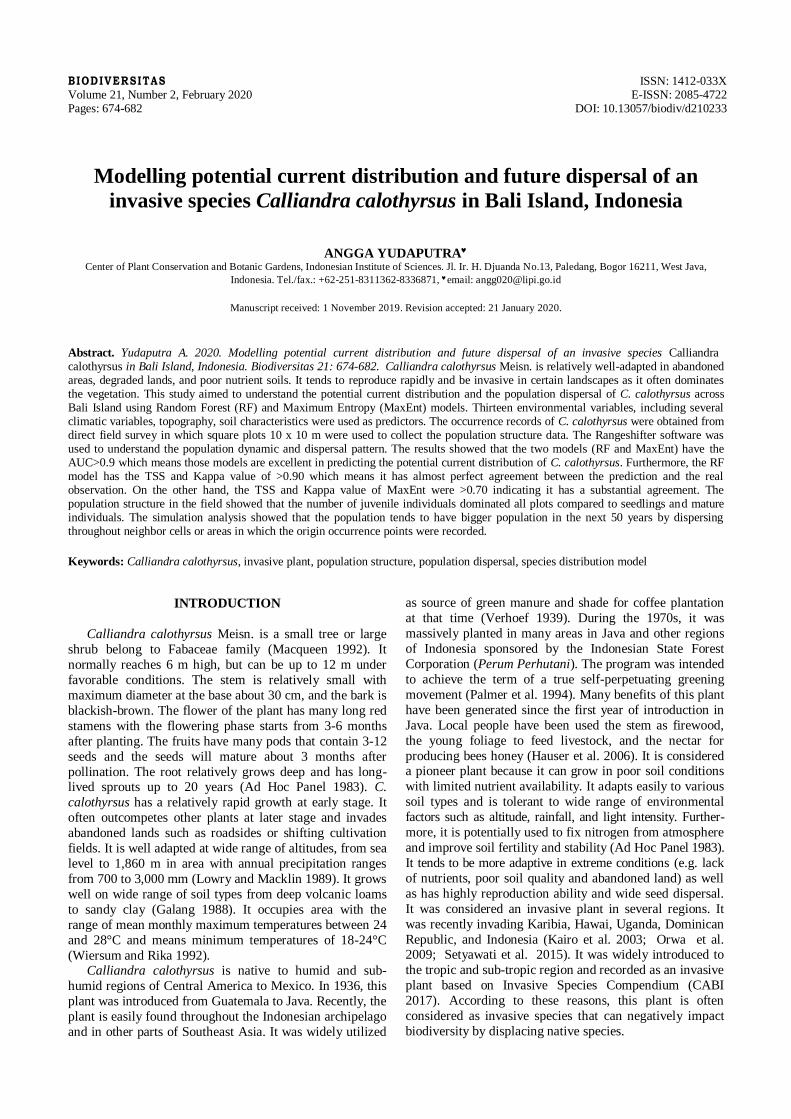
Figure 1. The morphology of Calliandra calothyrsus

Invasive species are defined as non-native or alien

species that occupy and dominates particular landscape or

ecosystem. Invasive plants are more likely to be successful

to establish and spread in a landscape because many

invasive plants are able to produce seeds in high quantities

which are easily dispersed by wind or birds. They can adapt to disturbed soil or abandoned land with poor soil

nutrients. Some invasive plants have aggressive root

systems that rapidly grow over large areas, some of them

produce chemical substances that inhibit other organisms to

live in its surrounding. The invasion of alien species in an

environment causes many problems, such as threatening

native species moreover the threatened and endangered

species, increasing the risk of soil erosion, and contributing

to the poor quality of agricultural lands (USDA 2019). For

landscape management purposes, understanding the

potential invasion of C. calothyrsus will be necessary as a consideration regarding proper management control. With

fairly rapid population growth, it needs to be monitored for

its development in the future. In terms of understanding the

distribution and dispersal of invasive alien species, the use

of species distribution modelling might be useful for

providing information regarding the mitigation and

management strategies. Predictive models of species

geographic distribution have been used in ecology and

conservation (Graham et al. 2004). There are many

application of species distribution modelling in ecology,

such as modelling the impact of climate change to species distribution (Thomas et al. 2004), modelling the spread

pattern of invasive species (Thuiller et al. 2005), and the

spatial pattern of species diversity (Graham et al. 2006).

Recently, many species distribution models have been

developed to understand the pattern of biodiversity

distribution.

Random forest (RF) is a machine learning that works based on regression and classification tree (Breiman 2001;

Liaw and Wiener 2002). RF is widely used in ecology

because it performs better as a classifier

(Cutler et al. 2007). Random Forest is a robust predictive

model that often used when the number of data points is

smaller compared to environmental predictors (Strobl

et al. 2007). RF outperforms than other species distribution

models (e.g. GLM, GAM, MARS, ANN) (Yudaputra et al.

2019). Furthermore, RF outperforms other predictive

models in predicting the distribution of Eusideroxylon

zwageri in Kalimantan (Yudaputra et al. 2020). Maximum Entropy (MaxEnt) is a modelling technique that can

achieve high predictive accuracy (Phillips and Dudik

2008). There are several advantages using MaxEnt, such as

it works both continuous and categorical data, it possibly

runs with presence only data, and overfitting can be

avoided (Phillips et al, 2006). In recent study, MaxEnt

shows the highest Area Under the Curve (AUC) value

compared to other species distribution models (e.g. RF,

SVM, GLM, BIOCLIM, DOMAIN) in predicting of

Guettarda speciosa (Yudaputra et al. 2019).

Area Under the Curve values (AUC) of receiver operator characteristic (ROC) curves, True Skill Statistics

BIODIVERSITAS 21 (2): 674-682, February 2020

676

(TSS), and Kappa statistic are used to measure the accuracy

of predictive models. The AUC is often used as a standard

to measure the accuracy of species distribution model

(Fielding and Bell 1997; Lobo et al. 2008). When the AUC

value > 0.5, it indicates the model works better than

random chance (Krzanowski and Hand 2009). The AUC

value represents how better model performance in which it

can be divided into several categories, i.e. 0.9-1 (excellent),

0.8-0.9 (good), 0.7-0.8 (fair), 0.6-0.7 (poor), and 0.5-0.6

(fail) (Krzanowski and Hand 2009). TSS is often used to evaluate the performance of model prediction and referred

to as Pierce skill score (Stephenson 2000). The TSS has the

range from-1 to +1 in which the value of +1 indicates

perfect agreement and value of zero or less indicates the

performance no better than random chance. The value of

TSS is categorized as follows, < 0.4 were poor, 0.4-0.8

useful, and > 0.8 good to excellent (Allouche et al. 2006).

Kappa represents the agreement between two binary

variables. Kappa is a measurement that also used in species

distribution modelling. The score of Kappa can be defined

as follows, 0 = agreement equivalent to chance, 0.1-0.20 = slight agreement, 0.21-0.40 = fair agreement, 0.41-0.60 =

moderate agreement, 0.61-0.80 = substantial agreement,

0.81-0.99 = near perfect agreement, 1 = perfect agreement

(Stephanie 2014).

Plant population dynamic refers to how the populations

change in their number through space and time by

quantifying their births, deaths, immigration, and

emigrations. The populations tend to exponentially increase

when they occupy in suitable conditions with freely

available resources. There are several factors that

determine the dynamic of population including demography, weather, soil condition, competitors,

herbivore, pathogen, and various hazards (fire) (Watkinson

1997). In case to understand the population growth and

dynamic, the use of matrices is strongly recommended. The

matrices in ecology that have been widely well known to

understand the population growth is Leslie matrix. It was

used to model the change of organisms in population over

period of time. The Leslie matrix works by dividing

population into several groups based on the age classes

(Caswell 2001). By combining the spatial analysis and

population demography, we could understand how the

population disperses in landscape. In study of invasive species, incorporating the correlative model and

mechanistic model would produce a useful predictive

model (Yudaputra 2019).

MATERIALS AND METHODS

Modelling potential current distribution

The current climatic variables were obtained from the

global climate data of the new version 2.0. Eight climatic

variables were chosen in this study: BIO1 = Annual Mean

Temperature, BIO4 = Temperature Seasonality (standard

deviation *100), BIO5 = Max Temperature of Warmest

Month, BIO6 = Min Temperature of Coldest Month, BIO12 = Annual Precipitation, BIO13 = Precipitation of

Wettest Month, BIO14 = Precipitation of Driest Month,

BIO15 = Precipitation Seasonality (Coefficient of

Variation). Those climatic data were available on raster

format (tiff) for all regions across the globe. The climatic

data are extracted from the global climatic data

(worldclim.org). The resolution 900 m (30 arc-second

resolution) was chosen for all climatic variables. Physical

environment variables were also used as a predictor in this

model. Those were elevation, soil pH, soil type, land cover,

and evapotranspiration. The topographic data are obtained

from the global data (earthexplorer.usgs.gov) and the soil data are extracted from soil grid global data (soilgrids.org).

Those variables were chosen because those are suspected

as physical environments that determining the distribution

pattern of this species. Both climatic and environmental

variables should have the same resolution that required to

run the species distribution modelling. The variables which

have finer resolution were downgraded as the other

variables. All spatial data in raster format (tiff) were

clipped to align with the study area (Bali). Those clipped-

climatic variables and physical environment variables were

then used for modelling process in R open sources. Two algorithms of species distribution model were used

to model potential current and future distribution of C.

calothyrsus. Those algorithms were Random Forest (RF)

and Maximum Entropy (MaxEnt). Several R packages

were used in this modelling such as “dismo” was used to

load climate variables, “randomforest” was used to run

Random Forest model, “rJava” was used to run the MaxEnt

model, “mapview” was used to see the point of

occurrences, library “sdm” was used to run several

algorithms of species distribution models. All algorithms

were run using “bootstrap” with two replications.

Field assessment of population structure

The population of Calliandra calothyrsus at secondary

forest in Pinggan village, Bangli District was used to

understand the population dynamic pattern. The population

of C. calothyrsus was grouped into several classes based on

its growth stage. Seedling individuals (0-2 m), juvenile

individuals (2-12 m), mature (individuals that entering the

flowering or fruiting phase). Ten plots with size 10 x 10 m

were established to record the individuals and group them

into several classes of growth stage. RANGESHIFTER

Ver.1.0 software was used to understand the population

dynamics of the species for 40 years.

Modelling population dispersal

Land use map of Indonesia was used to provide the

landscape feature in this model. The map consists of 17

types of land uses and covers all regions of Indonesia. The

polygon of the land use map was clipped with the base map

of Bali to extract only land-use of Bali. Then, the original

land use data projection (i.e. WGS 84) was converted into

UTM (Universal Transverse Mercator) coordinate

projection. The conversion of coordinate system is needed

because the RANGESHIFTER 1.0 requires inputs with

UTM projections. Then, the land use data as a polygon with UTM projection was converted into raster format. We

used 500 m resolution in spatial data preparation as inputs.

The last steps of spatial data preparation were converting


677

format of data from into asci as required in

RANGESHIFTER Software.

Point of occurrence data in XLXS or CSV (Comma

Delimited) format was loaded into GIS with the coordinate

projection was adjusted to UTM. The data was then

converted into shapefile (shp) of point occurrence. The

shapefile was converted into raster file format with a

resolution of 500 m. The last step, raster data was changed

into asci format as required in RANNGESHIFTER ver.1.0

software. Land use and point of occurrence should have the same coordinate projection and resolution as inputs of

software.

In RANGESHIFTER, the population dynamic data

should be fitted with several population parameters. The

Leslie matrix population would be helpful to understand

the population class. The probabilities of seedlings grow to

juvenile (G1 stage), the probabilities juvenile grow to

mature individual (G2 stage), the fecundity of mature

individual, the age required by mature individuals to

produce their offspring, and density dependence. We set

the probability of growing phase from seedling to juvenile as 0.6 and the probability of growing from juvenile to

mature individual as 0.3 in which both values were derived

from calculations. The minimum age of mature individuals

to reproduce offspring was approximately 5 years. The

survival probability was set to 0.8, and the fecundity of

mature individual was 90. The density independence was

set to 0.1 and mortality probability was 0.2. If the arrival

cells were unsuitable, the models will randomly choose a

suitable neighbor cell/grid. Mean distance of 500 m was

used in this dispersal model. The simulation was run for 2

replications. Two hundred individuals per cell were inputted in this model and the proportion of individuals per

stage 1 : stage 2 = 0.6 : 0.4. The simulation was run for 50

years to understand the dynamics of C. calothyrsus

population across the Bali landscape. The predictive

dynamic population maps were created every 10 years

throughout 50 years of simulation.

RESULTS AND DISCUSSION

Results

Two algorithms of species distribution models were

used to predict the potential current distribution of

Calliandra calothyrsus. In this study, three parameters of

model evaluation were used to evaluate model performance. Those were AUC value, True Skill Statistics

(TSS), and Kappa statistic. The AUC value of RF (0.98)

was better than that of MaxEnt (0.92) (Table 1). The two

models have the AUC value >0.90, indicating excellent

model performance in predicting the potential current

distribution. The TSS value of RF was much higher than

that of MaxEnt with 0.90 and 0.72 respectively. The TSS

value of RF >0.90 indicating that the performance of model

was excellent. On the other hands, the TSS value of

MaxEnt >0.70 indicating the model performance was good.

The last evaluation parameters used in this model were Kappa. The Kappa value of RF was 0.95 which means it

has almost perfect agreement between prediction and real

observation. Meanwhile, the Kappa value of MaxEnt was

0.79 indicating the model has substantial agreement. RF

predicted most accurately three predictors that determine

distribution patterns, which were elevation,

evapotranspiration, and precipitation (Figure 3).

Meanwhile, MaxEnt produced three most important

predictors including elevation, temperature, and

precipitation (Figure 4). The two models produced almost

similar predictive maps of potential current distribution of C. calothyrsus (Figures 5 and 6).

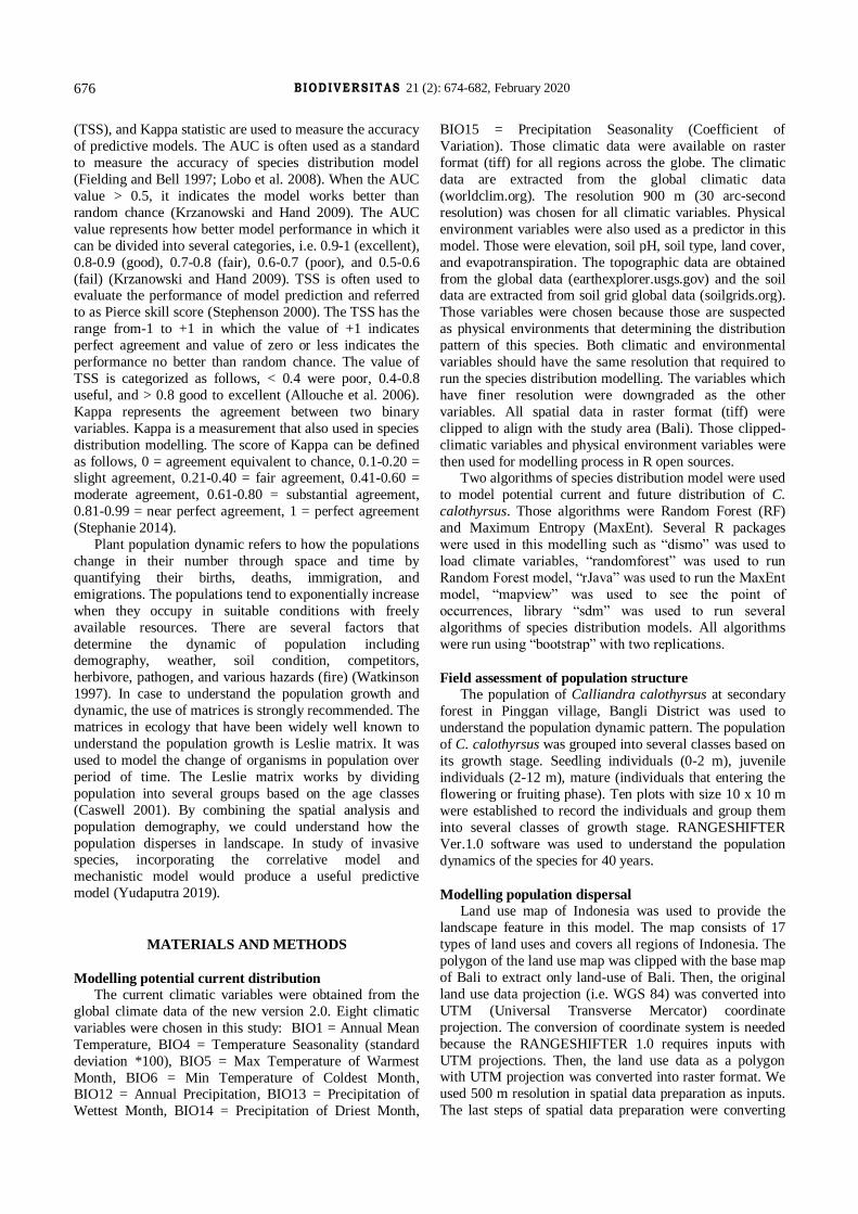
The results of our field survey showed that mature

individuals were relatively small in number compared to

seedlings and juvenile individuals in which only 3-5 mature

individuals were found at each plot. The juvenile

individuals were the most dominant in every plot. In

population structure analysis, the total of mature

individuals was 44, juvenile individuals 354, and seedlings

109 (Figure 7). Our simulation analysis indicated that

population tends to increase rapidly over 50 years of

simulation by dispersing in neighboring cells or locations. The population continuously growing for every ten years of

simulation.

Discussion

Species Distribution Models (SDMs) were often used to

understand the potential distribution area of a species by

incorporating physical environment variables and presence

only records or presence-absence records. In this study,

thirteen environmental variables were used to run this

model because those variables were presumably important

in terms of determining the distribution pattern. The

selection of environmental variables should consider the presence requirement of the species. The selection of

environmental variables was a critical way of determining

the accuracy of predictive model. In model calibration,

dataset was divided into training and testing data in which

training data was used for developing the model, whereas

the testing data was used for evaluating the model

performance. The testing data for evaluation was ideally

obtained from resampling which was considered as

independent data. However, splitting data was often

considered as the best solution since the time and effort to

resample the data were limited. In our analysis, we used the

proportion of training data: testing data = 75 : 25. Based on the results of this study, according to three parameters of

evaluation (i.e. AUC, TSS, Kappa), the predictive models

produced by RF and MaxEnt were categorized as excellent

predictive models. Those models were highly

recommended to be used in prediction of potential

distribution. Table 1. The evaluation of model performance using the AUC, TSS, and Kappa

Methods AUC TSS Kappa

Random Forest (RF) 0.98 0.90 0.95 Maximum Entrophy (MaxEnt) 0.92 0.72 0.79


678

Figure 2. The ROC and AUC value: A. Random Forest (RF); B. Maximum Entropy (MaxEnt)

Figure 3. The relative importance of environment variables using Random Forest (RF)

Figure 4. The relative importance of environmental variables using Maximum Entropy (MaxEnt)


679

Figure 5. The predictive map of potential current distribution of Calliandra calothyrsus using Random Forest (RF)

Figure 6. The predictive map of potential current distribution of Calliandra calothyrsus using MaxEnt

A B C

Figure 7. The population structure of Calliandra calothyrsus: A. Seedlings, B. Juvenile individuals, C. Mature individuals

140

120

100

80

60

40

20

0

0.2 2.4 4.6 6.8 8.10 10.12 12.14 14.16

Height (m)

No

. of

ind

ivid

ual

s

140

120

100

80

60

40

20

0

0.2 2.4 4.6 6.8 8.10 10.12 12.14 14.16

Height (m)

No

. of

ind

ivid

ual

s

140

120

100

80

60

40

20

0

0.2 2.4 4.6 6.8 8.10 10.12 12.14 14.16

Height (m)

No

. of

ind

ivid

ual

s


680

1

2

3

Year_20 Year_30

Year_40

Year_0

Year_50

Year_10

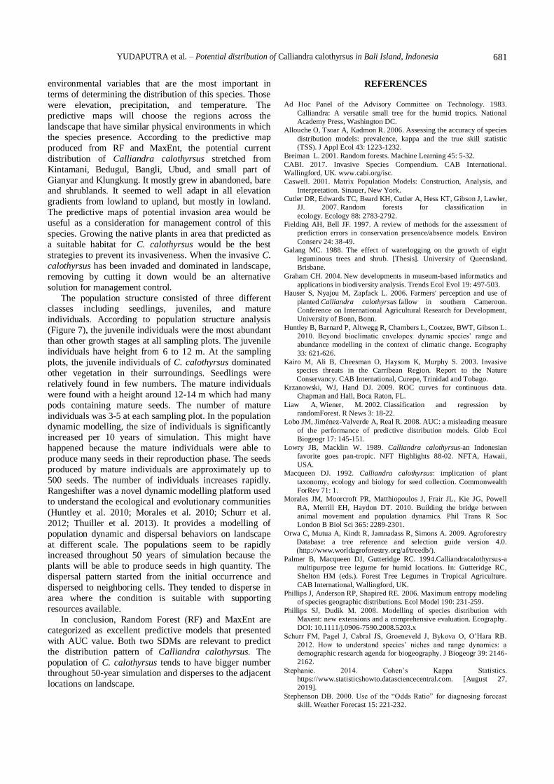
Figure 9. The population dispersal of Calliandra calothyrsus across Bali landscape. The orange color presents the growth of population of Calliandra calothyrsus throughout 50 years simulation

Figure 10. Population dynamic of Calliandra calothyrsus throughout 50 years of simulation

Random Forest (RF) and Maximum Entropy (MaxEnt)

were chosen because those models outperform to other

SDMs models. MaxEnt produced the highest AUC value,

followed by SVM and RF in predicting of Zebra Wood

distribution (Yudaputra et al. 2019). Both two predictive

models (RF and MaxEnt) produced almost similar


681

environmental variables that are the most important in

terms of determining the distribution of this species. Those

were elevation, precipitation, and temperature. The

predictive maps will choose the regions across the

landscape that have similar physical environments in which

the species presence. According to the predictive map

produced from RF and MaxEnt, the potential current

distribution of Calliandra calothyrsus stretched from

Kintamani, Bedugul, Bangli, Ubud, and small part of

Gianyar and Klungkung. It mostly grew in abandoned, bare and shrublands. It seemed to well adapt in all elevation

gradients from lowland to upland, but mostly in lowland.

The predictive maps of potential invasion area would be

useful as a consideration for management control of this

species. Growing the native plants in area that predicted as

a suitable habitat for C. calothyrsus would be the best

strategies to prevent its invasiveness. When the invasive C.

calothyrsus has been invaded and dominated in landscape,

removing by cutting it down would be an alternative

solution for management control.

The population structure consisted of three different classes including seedlings, juveniles, and mature

individuals. According to population structure analysis

(Figure 7), the juvenile individuals were the most abundant

than other growth stages at all sampling plots. The juvenile

individuals have height from 6 to 12 m. At the sampling

plots, the juvenile individuals of C. calothyrsus dominated

other vegetation in their surroundings. Seedlings were

relatively found in few numbers. The mature individuals

were found with a height around 12-14 m which had many

pods containing mature seeds. The number of mature

individuals was 3-5 at each sampling plot. In the population dynamic modelling, the size of individuals is significantly

increased per 10 years of simulation. This might have

happened because the mature individuals were able to

produce many seeds in their reproduction phase. The seeds

produced by mature individuals are approximately up to

500 seeds. The number of individuals increases rapidly.

Rangeshifter was a novel dynamic modelling platform used

to understand the ecological and evolutionary communities

(Huntley et al. 2010; Morales et al. 2010; Schurr et al.

2012; Thuiller et al. 2013). It provides a modelling of

population dynamic and dispersal behaviors on landscape

at different scale. The populations seem to be rapidly increased throughout 50 years of simulation because the

plants will be able to produce seeds in high quantity. The

dispersal pattern started from the initial occurrence and

dispersed to neighboring cells. They tended to disperse in

area where the condition is suitable with supporting

resources available.

In conclusion, Random Forest (RF) and MaxEnt are

categorized as excellent predictive models that presented

with AUC value. Both two SDMs are relevant to predict

the distribution pattern of Calliandra calothyrsus. The

population of C. calothyrsus tends to have bigger number throughout 50-year simulation and disperses to the adjacent

locations on landscape.

REFERENCES

Ad Hoc Panel of the Advisory Committee on Technology. 1983.

Calliandra: A versatile small tree for the humid tropics. National

Academy Press, Washington DC.

Allouche O, Tsoar A, Kadmon R. 2006. Assessing the accuracy of species

distribution models: prevalence, kappa and the true skill statistic

(TSS). J Appl Ecol 43: 1223-1232.

Breiman L. 2001. Random forests. Machine Learning 45: 5-32.

CABI. 2017. Invasive Species Compendium. CAB International.

Wallingford, UK. www.cabi.org/isc. Caswell. 2001. Matrix Population Models: Construction, Analysis, and

Interpretation. Sinauer, New York.

Cutler DR, Edwards TC, Beard KH, Cutler A, Hess KT, Gibson J, Lawler,

JJ. 2007. Random forests for classification in

ecology. Ecology 88: 2783-2792.

Fielding AH, Bell JF. 1997. A review of methods for the assessment of

prediction errors in conservation presence/absence models. Environ

Conserv 24: 38-49.

Galang MC. 1988. The effect of waterlogging on the growth of eight

leguminous trees and shrub. [Thesis]. University of Queensland,

Brisbane.

Graham CH. 2004. New developments in museum‐based informatics and

applications in biodiversity analysis. Trends Ecol Evol 19: 497-503.

Hauser S, Nyajou M, Zapfack L. 2006. Farmers' perception and use of

planted Calliandra calothyrsus fallow in southern Cameroon.

Conference on International Agricultural Research for Development,

University of Bonn, Bonn.

Huntley B, Barnard P, Altwegg R, Chambers L, Coetzee, BWT, Gibson L.

2010. Beyond bioclimatic envelopes: dynamic species’ range and

abundance modelling in the context of climatic change. Ecography

33: 621-626.

Kairo M, Ali B, Cheesman O, Haysom K, Murphy S. 2003. Invasive

species threats in the Carribean Region. Report to the Nature

Conservancy. CAB International, Curepe, Trinidad and Tobago. Krzanowski, WJ, Hand DJ. 2009. ROC curves for continuous data.

Chapman and Hall, Boca Raton, FL.

Liaw A, Wiener, M. 2002. Classification and regression by

randomForest. R News 3: 18-22.

Lobo JM, Jiménez-Valverde A, Real R. 2008. AUC: a misleading measure

of the performance of predictive distribution models. Glob Ecol

Biogeogr 17: 145-151.

Lowry JB, Macklin W. 1989. Calliandra calothyrsus-an Indonesian

favorite goes pan-tropic. NFT Highlights 88-02. NFTA, Hawaii,

USA.

Macqueen DJ. 1992. Calliandra calothyrsus: implication of plant

taxonomy, ecology and biology for seed collection. Commonwealth

ForRev 71: 1.

Morales JM, Moorcroft PR, Matthiopoulos J, Frair JL, Kie JG, Powell

RA, Merrill EH, Haydon DT. 2010. Building the bridge between

animal movement and population dynamics. Phil Trans R Soc

London B Biol Sci 365: 2289-2301.

Orwa C, Mutua A, Kindt R, Jamnadass R, Simons A. 2009. Agroforestry

Database: a tree reference and selection guide version 4.0.

(http://www.worldagroforestry.org/af/treedb/). Palmer B, Macqueen DJ, Gutteridge RC. 1994.Calliandracalothyrsus-a

multipurpose tree legume for humid locations. In: Gutteridge RC,

Shelton HM (eds.). Forest Tree Legumes in Tropical Agriculture.

CAB International, Wallingford, UK.

Phillips J, Anderson RP, Shapired RE. 2006. Maximum entropy modeling

of species geographic distributions. Ecol Model 190: 231-259.

Phillips SJ, Dudik M. 2008. Modelling of species distribution with

Maxent: new extensions and a comprehensive evaluation. Ecography.

DOI: 10.1111/j.0906-7590.2008.5203.x

Schurr FM, Pagel J, Cabral JS, Groeneveld J, Bykova O, O’Hara RB.

2012. How to understand species’ niches and range dynamics: a

demographic research agenda for biogeography. J Biogeogr 39: 2146-

2162.

Stephanie. 2014. Cohen’s Kappa Statistics.

https://www.statisticshowto.datasciencecentral.com. [August 27,

2019].

Stephenson DB. 2000. Use of the “Odds Ratio” for diagnosing forecast

skill. Weather Forecast 15: 221-232.


682

Strobl C, Boulesteix AL, Zeileis A, Hothorn T. 2007. Bias in random

forest variable importance measures: Illustrations, sources and a

solution. BMC Bioinformatics 8: 25. DOI: 10.1186/1471-2105-8-25.

Thomas CD, Cameron A, Green R, et al. 2004. Extinction risk from

climate change. Nature 427: 145-148.

Thuiller W, David R, Petr P, Midgley G, Hughes G, Rouget

M. 2005. Niche‐based modelling as a tool for predicting the risk of

alien plant invasions at a global scale. Glob Ch Biol 11: 2234-2250.

Thuiller W, Münkemüller T, Lavergne S, Mouillot D, Mouquet N,

Schiffers K, Gravel D. 2013. A road map for integrating eco-

evolutionary processes into biodiversity models. Ecol Lett 16: 94-105.

United States Department of Agriculture (USDA). 2019. Invasive Plants.

https://www.fs.fed.us/wildflowers/invasives/index.shtml. [August 26,

2019].

Verhoef L. 1939. Calliandra calothyrsus Meissn. Korte Mededeelingen

79. Boschbouwproefstation, Bogor, Java, Indonesia. [Dutch]

Watkinson AR. 1997. Population dynamics. In: Crawley MJ (ed.). Plant

Ecology. Blackwell Scientific Publications, Oxford.

Wiersum KF, Rika IK. 1992. Calliandra calothyrsus Meissn. In: Westphal

E, Jansen PCM (eds), Plant Resources of Southeast Asia: 4 Forages.

PudocWageningen, Netherlands.

Yudaputra A, Astuti IP, Cropper WP. 2019. Comparing six different

species distribution models with several subsets of environmental

variables: Predicting the potential current distribution of Guettarda

speciosa in Indonesia. Biodiversitas 20 (8): 2321-2328.

Yudaputra A, Rinandio DS, Sudarmono. 2019. Projecting the niche

(suitable habitats) of invasive species: approaches, challenges, and

consequences. Proceedings of The 3rd SATREPS Conference.

Yudaputra A, Robiansyah I, Rinandio DS. 2019. the implementation of

artificial neural network and random forest in ecological research:

species distribution modelling with presence and absence dataset.

Proceedings of The 3rd SATREPS Conference.

Yudaputra A, Fijridiyanto I, Cropper WP Jr. 2020. The potential impact of

climate change on the distribution pattern of Eusideroxylon zwageri

(Bornean Ironwood) in Kalimantan, Indonesia. Biodiversitas 21(1):

326-333.

modelling potential current distribution and future

Documents