1

Modelling of tsunami-induced bore and structure interaction

Authors

Gede Pringgana MEng, A.M.ASCE PhD Student, School of Mechanical, Aerospace and Civil Engineering,

University of Manchester, Manchester, UK.

Lee S. Cunningham MEng, PhD, CEng, MICE, MIStructE Lecturer, School of Mechanical Aerospace and Civil Engineering,

University of Manchester, Manchester, UK

Benedict D. Rogers MEng (Oxon), DPhil Reader, School of Mechanical, Aerospace and Civil Engineering,

University of Manchester, Manchester, UK

ABSTRACT

A series of 3-D smoothed particle hydrodynamics (SPH) and finite element (FE) models with

a domain in the form of a water tank were undertaken to simulate tsunami-induced bore

impact on a discrete onshore structure on a dry bed. The fluid motion was simulated using the

SPH-based software DualSPHysics. The tsunami-like waves were represented by solitary

waves with different characteristics generated by the numerical paddle wavemaker.

Numerical probes were uniformly distributed on the structure’s vertical surface providing

detailed measures of the pressure distribution across the structure. The peak impact locations

on the structure’s surface were specifically determined and the associated peak pressures then

compared with the prediction of existing commonly used design equations. Using the

pressure-time histories from the SPH model, FE analysis was conducted with ABAQUS to

model the dynamic response of a representative timber structure. The results show that the

equations used to estimate the associated pressure for design purposes can be highly non-

conservative. By gaining a detailed insight into the impact pressures and structure response,

engineers have the potential means to optimise the design of structures under tsunami impact

loads and improve survivability.

Keywords: coastal engineering, hydraulics & hydrodynamics, timber structures, SPH

1. Introduction

In many parts of the world, structures in low lying coastal areas are at risk of tsunami

inundation and can suffer significant damage if they are not adequately designed for the

associated hydrodynamic loads. Onshore tsunami waves propagate from the deep ocean

towards the shoreline and break when the incident wave height is approximately similar with

the water depth. A broken tsunami wave moves inland in the form of a turbulent hydraulic

bore (Palermo et al., 2009) as captured on video footage of the 26 December 2004 Indian

Ocean Tsunami (Nouri et al., 2010). In the context of this work, a bore is defined as a steep,

2

rapidly moving broken wave with an onshore mass flux that can be very destructive (IOC,

2013).

In the major tsunami disasters in 2004 and 2011 the tsunami bore inundation greatly

affected shore-based structures including many critical pieces of infrastructure such as

railways, nuclear facilities, etc. By far the majority of structures damaged or destroyed in

these events were residential buildings. After the 2011 East Japan tsunami, Suppasri et al.

(2013) stated that 115,163 houses were heavily damaged, 162,015 houses were moderately

damaged and 559,321 houses were partially damaged. Many of those houses were

constructed from timber. Such timber structures might survive the earthquake that generated

the tsunami due to their relatively high strength-to-mass ratio and flexibility but could not

resist the hydrodynamic forces resulting from the bore impact.

An improved understanding of residential building response to tsunami loads could

help reduce casualties, increase survive-ability of such structures and speed up recovery time

post-tsunami. Becker et al. (2011) show that a key factor of building response to the external

actions is the interaction between the structural components of the building and the wave.

The pressure of the tsunami bore can be likened to the pressures attributable to winds which

are treated as uniform lateral pressures acting along the entire height of the building.

However, in determining tsunami loads, the varying depth of the water, associated velocity

and duration of impact are added variables that affect the resulting force and structure

response.

Existing design codes and guides around the world present various approaches to

quantification of tsunami loads on buildings. The City and County of Honolulu Building

Code (CCH, 2000) recommends formulation as shown by Equation (1), adopted from Dames

and Moore (1980), to predict hydraulic bore-like wave impact on vertical walls. The

Structural Design Method of Buildings for Tsunami Resistance (SMBTR) in Japan developed

by Okada et al. (2005) also assumed surge force as given by Equation (1). The surge force

(𝐹𝑠) given in Equation (1) results from the summation of hydrostatic and hydrodynamic force

components as given by the following expression:

𝐹𝑠 = 1

2𝜌𝑔ℎ2𝑏 +

1

2𝐶𝑑𝜌𝑢2ℎ𝑏 (1)

where 𝐹𝑠 is the surge force per unit width of wall, 𝜌 is the density of water, 𝑔 is the

gravitational acceleration, ℎ is the surge height usually assumed equal to the inundation depth

or flood level, 𝑏 is the breadth of impacted structure, 𝐶𝑑 is the drag coefficient which is

recommended by FEMA 55 (2003) and CCH (2000) as being equal to 2.0 for the case of

square or rectangular piles and 𝑢 is the tsunami flow velocity. The general form of the

tsunami-induced flow velocity is 𝑢 = 𝐶√𝑔ℎ, where 𝐶 is a constant coefficient which is

assumed by FEMA 55 (2003) and Camfield (1980) as having a value of 2. The substitution of

𝑢 = 2√𝑔ℎ into Equation (1) results in the surge force (Fs) as follows:

𝐹𝑠 = 1

2𝜌𝑔ℎ2𝑏 + 4 𝜌𝑔ℎ2𝑏 = 4.5𝜌𝑔ℎ2𝑏 (2)

Fujima et al. (2009) also proposed two equations for a dry flat shoreline configuration

based on the maximum water inundation level and the distance of the structure from the

3

shoreline. The equation expresses the distance of structure from shoreline (DF) in terms of

(him/DF), where him is the maximum inundation depth. For the numerical model presented

here the condition where him/DF > 0.05 is satisfied, the structure is categorized as close to the

shoreline, thus the equation that is applicable for an average estimation of force is:

𝐹 = 1.8𝜌𝑔ℎ𝑖𝑚𝐵 (3)

in which B is the breadth of structure. As an appropriate safety factor, Fujima et al. (2009)

suggests the coefficient of 1.8 in Equation (3) be increased to 3.3. These equations have

resulted from small-scale physical experiments for bores propagating over a dry bed.

Robertson et al. (2011) categorized the main research on wave impact loads on

structures into the following three areas: (i) work related with storm wave impact on offshore

platforms which is presently the most commonly studied; (ii) combining experimental and

numerical research in order to develop design formulae for associated loads on structures;

(iii) research on the forces and associated structural response resulting from tsunami bores

impacting on land-based structures. This last area, is least studied. Consequently, there is a

need for better understanding of tsunami bore impact on onshore coastal structures due to the

relatively limited available research. Following the Indian Ocean tsunami in 2004 and the

Tohoku tsunami in 2011, extensive study has been conducted in order to improve the

understanding tsunami impact loads and improve design guidelines. However, research has

mainly focused on experimental investigation and has been mostly confined to small scale

models, while numerical models have been limited due to the high computational demand

(Como and Mahmoud, 2013). The research presented herein is intended to address the

aforementioned issues by providing more detailed information on tsunami-induced bore and

structure interactions via numerical models. The numerical study is conducted using two

software packages: (i) the fluid is simulated using the smoothed particle hydrodynamics

(SPH) software DualSPHysics; DualSPHysics is a free open-source SPH code released online

(see http://www.dual.sphysics.org), (ii) the structural response is simulated using the

commercial software ABAQUS. The ultimate goal of the research is to enhance present

understanding of tsunami wave-structure interaction with a view to improving current design

provisions.

Smoothed particle hydrodynamics is a meshless Lagrangian technique which is ideal

for simulating highly nonlinear free-surface phenomena such as tsunami waves. By solving

the 3-D Navier-Stokes equations, the SPH numerical modelling technique offers the potential

for improved definition of wave characteristics and associated pressures on impacted

structures. The capabilities of SPH to model wave-structure interaction for coastal

engineering problems were presented by Dalrymple et al. (2009), Barreiro et al. (2013) and

Altomare et al. (2015). Previous studies by the authors have demonstrated the applicability of

SPH in quantifying tsunami wave characteristics within acceptable levels of accuracy when

impacting vertical onshore structures (Cunningham et al., 2014). In addition to the laboratory

experiments on tsunami wave impact on structures near shore, St-Germain et al. (2014) also

conducted the numerical modelling using SPH on the basis of analogies between tsunami

bores and dam break waves. Furthermore, the SPH technique has also been used to model

other violent wave behaviour such as storm wave impact on vertical walls near shore,

4

(Altomare et al., 2015). More details about DualSPHysics program can be found in Crespo et

al. (2015), Crespo et al. (2011), Crespo et al. (2013), Gomez-Gesteira et al. (2012a), Gomez-

Gesteira et al. (2012b). Although Canelas et al. (2013) have coupled SPH to the discrete

element method (DEM) for fluid-structure interaction none of the aforementioned studies

have investigated the response of a deformable structure due to the hydrodynamics of a

tsunami-like wave. This paper addresses that gap building on the work of (Cunningham et al.,

2014).

This paper is structured as follows; firstly an overview of the two stages of numerical

modelling is given. This is followed by the detailed description of the SPH modelling

including model geometry and associated convergence study. Subsequent to this the results

from the SPH models including the pressure-time histories that will be applied in the finite

element model will be described. Finally, the response of the impacted structures via finite

element analysis will be presented and discussed.

2. Methodology

The numerical modelling conducted herein consists of two stages, the first being the

simulation of tsunami-like waves followed by the modelling of the response of the wave-

impacted structure. The numerical simulations of the tsunami-like wave were conducted

using DualSPHysics version 3.0 and were intended to predict tsunami-like bore pressure

distributions on the surface of impacted structures. The output obtained from SPH numerical

modelling in the form of wave pressure distribution histories are then used as an input in the

second stage numerical modelling using the commercially available finite element software

ABAQUS/CAE 6.10 to define the structural response of an idealized residential structure.

DualSPHysics can perform SPH computational modelling on both central processing units

(CPUs) and Graphics Processing Units (GPUs). Hardware acceleration provided by a GPU

was performed to take advantage of speed ups of up to two orders of magnitude. In addition

to previous studies undertaken by the authors, further validation of the SPH model was

conducted by re-modelling the dambreak simulation by Kleefsman et al. (2005).

For simulation purposes, throughout this work the tsunami wave is idealised as a

solitary wave. This is an idealisation taking advantage of the well-defined and reproducible

characteristics of a solitary wave. For discussion on the merits of this approach, the reader is

referred to McCabe et al. (2014). The variation of solitary wave height, H, was non-

dimensionalised using the offshore water depth h0. Three different cases with different

solitary wave heights were performed, H/h0 = 0.1, 0.3 and 0.5. Other parameters in the

modelling were kept constant. The H/h0 values were expected to give associated bores with

specific heights and velocities that are two main factors in the determination of bore impact

pressure on onshore structures. The numerical pressures output from each numerical case will

be compared with the pressures determined from existing empirical equations that are based

on physical experiments for bores propagating over a dry bed.

5

The tsunami-like wave simulation presented herein uses a small-scale domain. To

implement the numerical modelling results in a real condition, normal similarity Froude

scaling laws are applied. For practical purposes, the size of idealized structure in the

numerical SPH model (1m x 1m x 1m) was scaled up by a factor of 3, where this value was

chosen to resemble the feasible size of simple single storey residential shelter made of timber.

In line with Froude scaling laws, the SPH pressure output was also scaled up by a factor of 3.

The structure’s dimensions and the pressure loads after being scaled are then used in the

finite element (FE) model. These types of structure were chosen as the focus of the FE

modelling because they are fairly typical of the coastal buildings widely damaged by the

tsunamis of 2004 and 2011 (Como and Mahmoud, 2013; Suppasri et al., 2013). The

dimensions and material properties of the representative timber structure’s members in the FE

model follow the provisions set out in the International Residential Code (ICC, 2009). More

details on SPH and FE modelling are explained in the following sections.

3. Description of the SPH Models

The SPH method is based on integral interpolants. Following Barreiro et al. (2013),

the fundamental principle is to approximate any function 𝐴(𝒓) by:

⟨𝐴(𝒓)⟩ = ∫ 𝐴(𝒓)𝑊(𝒓 − 𝒓′, ℎ)𝑑𝒓′

Ω

(4)

where 𝒓 is position, 𝑊 is the weighting function or kernel, ℎ is the or smoothing length

which controls the radius of influence of domain of Ω and ... denotes an approximation.

Equation (4), in discrete notation, leads to an approximation of the function at a particle of

interest (interpolant point) 𝑎:

𝐴𝑎 = ∑ 𝐴𝑏

𝑚𝑏

𝜌𝑏𝑏

𝑊𝑎𝑏 (5)

where the subscript refers to each particle, 𝑚 is the mass, and 𝜌 is density and the summation

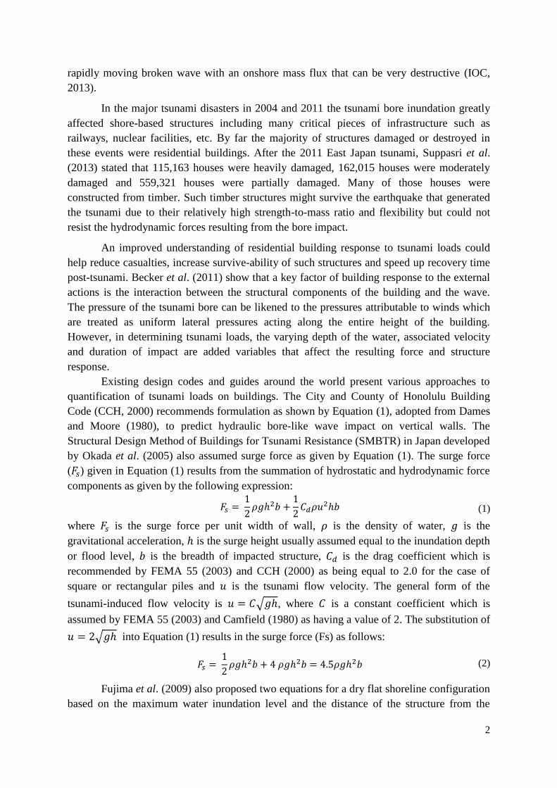
is performed over all the particles 𝑏 within the region of compact support of the kernel

function as illustrated by Figure 1.

Figure 1 Schematic of the SPH smoothing kernel

particle of interest

rab

neighbour particle

W(rab , h)kernel

ab2h

rab

radius of influence

waterparticle

6

The SPH model relies on the selection of the weighting functions that must satisfy the

conditions such as positivity, compact support and normalization (Monaghan, 1992). When

evaluated for the interaction between two particles 𝑎 and 𝑏 the weighting function, 𝑊𝑎𝑏,

depends on the smoothing length, h, and is normally expressed in terms of the non-

dimensional distance between particles given by 𝑞 = 𝑟𝑎𝑏 ℎ⁄ where 𝑟𝑎𝑏 is the distance between

particles 𝑎 and b (𝑟𝑎𝑏 = |𝒓𝑎 − 𝒓𝑏|). The parameter ℎ controls the size of the area

surrounding particle 𝑎 where the contribution of any other particles inside the area cannot be

neglected. In the SPH simulations presented in this paper, the fifth-order Wendland kernel is

used. More information on the kernels and the formulation available in DualSPHysics can

found in Crespo et al. (2015).

As in many weakly compressible SPH (WCSPH) simulations, the kernel

approximation and its gradient are not corrected to ensure reproducibility of the constant and

linear functions. Although kernel correction is attractive mathematically, and in some SPH

formulations essential (notably the incompressible SPH (ISPH) simulations where

conservation is discarded in favour of increased accuracy, Lind et al. (2012)), it is not

essential for WCSPH simulations since the SPH equations conserve the fundamental

quantities of mass and momentum (Violeau and Rogers, 2016). Indeed, enforcing

reproducibility can make WCSPH unstable while Altomare et al. (2015), Barreiro et al.

(2013), Farahani et al. (2014) and St-Germain et al. (2014) have shown that WCSPH with no

correction gives satisfactory results for nearshore wave processes.

The SPH formalism is used to discretise the governing equations expressing conservation of

mass and momentum.

Conservation of Mass

In WCSPH, the conservation of mass equation, or continuity, is solved in Lagrangian

form as:

𝑑𝜌

𝑑𝑡= − 𝜌∇. 𝝊 (6)

where 𝒗 is the velocity, 𝑡 is time and 𝜌 is density. The changes in the fluid particle density

are determined by solving the conservation of mass or continuity equation in SPH form:

𝑑𝜌𝑎

𝑑𝑡= ∑ 𝑚𝑏𝒗𝑎𝑏 ∙ ∇𝑎𝑊𝑎𝑏

𝑏

(7)

where 𝒗𝑎𝑏 = 𝒗𝑎 − 𝒗𝑏 and ∇𝑎𝑊𝑎𝑏, denotes the derivative of the smoothing kernel 𝑊𝑎𝑏 with

respect to the coordinates of particle 𝑎 . The mass of each SPH particle is kept constant.

Conservation of Momentum

In Lagrangian form, the momentum equation in continuous form is:

𝑑𝒗

𝑑𝑡= −

1

𝜌∇𝑃 + 𝒈 + 𝜞 (8)

7

where 𝑃 is pressure, 𝒈 = (0, 0, -9.81) ms-2

is the gravitational acceleration and 𝜞 is the

dissipative terms. There are several ways to solve the dissipative terms; however, the most

widely used due to its simplicity is the artificial viscosity proposed by Monaghan (1992) and

is used herein.

There are numerous forms of an SPH gradient which are chosen according to the

physics or numerical properties. With the classical formulation, the pressure gradient in SPH

notation uses a symmetric form of the gradient to conserve momentum:

−

1

𝜌∇𝑃 = − ∑ 𝑚𝑏 (

𝑃𝑎

𝜌𝑎2

+𝑃𝑏

𝜌𝑏2) ∇𝑎𝑊𝑎𝑏

𝑏

(9)

where 𝑃𝑏 and 𝜌𝑏 are pressure and density of particle 𝑏. The artificial viscosity can be

included in Equation (9) by adding the viscosity term 𝜫𝑎𝑏 inside the bracket. Thus, the

momentum conservation equation in SPH will be:

𝑑𝒗𝑎

𝑑𝑡= − ∑ 𝑚𝑏 (

𝑃𝑎

𝜌𝑎2

+𝑃𝑏

𝜌𝑏2 + 𝜫𝑎𝑏) ∇𝑎𝑊𝑎𝑏

𝑏

+ 𝒈 (10)

The artificial viscosity depends on the relative position and motion of the computed particles

𝜫𝑎𝑏 = {

−𝛼𝑐𝑎𝑏̅̅ ̅̅ 𝜇𝑎𝑏

𝜌𝑎𝑏

0

𝒗𝑎𝑏 ∙ 𝒓𝑎𝑏 < 0

𝒗𝑎𝑏 ∙ 𝒓𝑎𝑏 > 0

(11)

where 𝒗𝑎𝑏 = 𝒗𝑎 − 𝒓𝑏, 𝜇𝑎𝑏 = ℎ𝒗𝑎𝑏 ∙ 𝒓𝑎𝑏/(𝒓𝑎𝑏2 + 𝜂2), 𝑐𝑎𝑏 = 0.5 (𝑐𝑎 + 𝑐𝑏) is the mean value

of the speed of sound, 𝜂2 = 0.01 ℎ2, and 𝛼 is a parameter whose value ranges from 0.01 to

0.5, that should be adjusted according the configuration of the problem.

In the simulations presented herein, a 3-D SPH numerical water tank is used for simulating

near-shore and onshore areas. In DualSPHysics, the implemented boundary conditions

include the Dynamic Boundary Conditions (DBCs) for solid walls (Crespo et al., 2007) and

the Periodic Boundary Conditions (PBCs) for lateral open boundaries (Gomez-Gesteira et al.,

2012). To represent a solid wall, the dynamic SPH boundary was used for the numerical

model. The boundary particles (BPs) and the fluid particles (FPs) in the DBCs satisfy the

same equations but are not allowed to move (the movement is equal to zero) in any direction

except where externally imposed such as a flap or a piston in a wave maker. In the

DualSPHysics code, the initial geometry, configuration and case parameters are defined in

the Extensible Markup Language (XML) input file and this also includes the size of particles.

In the following subsections, first the particle size required to capture the pressure due to the

bore impact is identified, and second, this information is then used to model the tsunami bore

impacting the structure.

3.1 Choosing the particle size (dp): convergence study for bore impact.

The choice of water particle size or the initial spacing of particle (𝑑𝑝) is crucial in

SPH modelling. The particle size influences the overall simulation including the behaviour of

8

waves, the accuracy of pressure prediction and the time of simulation. The particle size was

determined using a numerical convergence study by re-modelling the dambreak impact on a

box case in Kleefsman et al. (2005) as suggested by the SPH European Research Interest

Community (SPHERIC) for relevant model validation. The use of the dambreak case for

validation purposes is based on the assumption that the bore characteristics of the tsunami are

closely represented by a broken dambreak wave front (Chanson, 2006). This case has been

used previously for validation to demonstrate convergence (Crespo et al., 2011), here the

maximum particle size required to capture the impact pressures is identified.

The fluid flow properties in the convergence study were the impact pressure and the

water level. Many parameters influence the pressure and the water level but in this case their

values were kept constant for all models and only the particle size (dp) was modified

following previous work by the authors, (Cunningham et al., 2014). The only execution

parameter recently added in this model is the “-SPH” where the value was equal to 0.1. The

-SPH is one of some improvement in DualSPHysics version 3 that was used for all SPH

models in this paper. The -SPH scheme virtually eliminates unphysical pressure fluctuations

and thereby enhances the pressure prediction of an SPH model involving violent waves.

A convergence study is needed to determine the largest particle size and hence

shortest runtime that can use in a simulation to capture hydrodynamics. The shortest

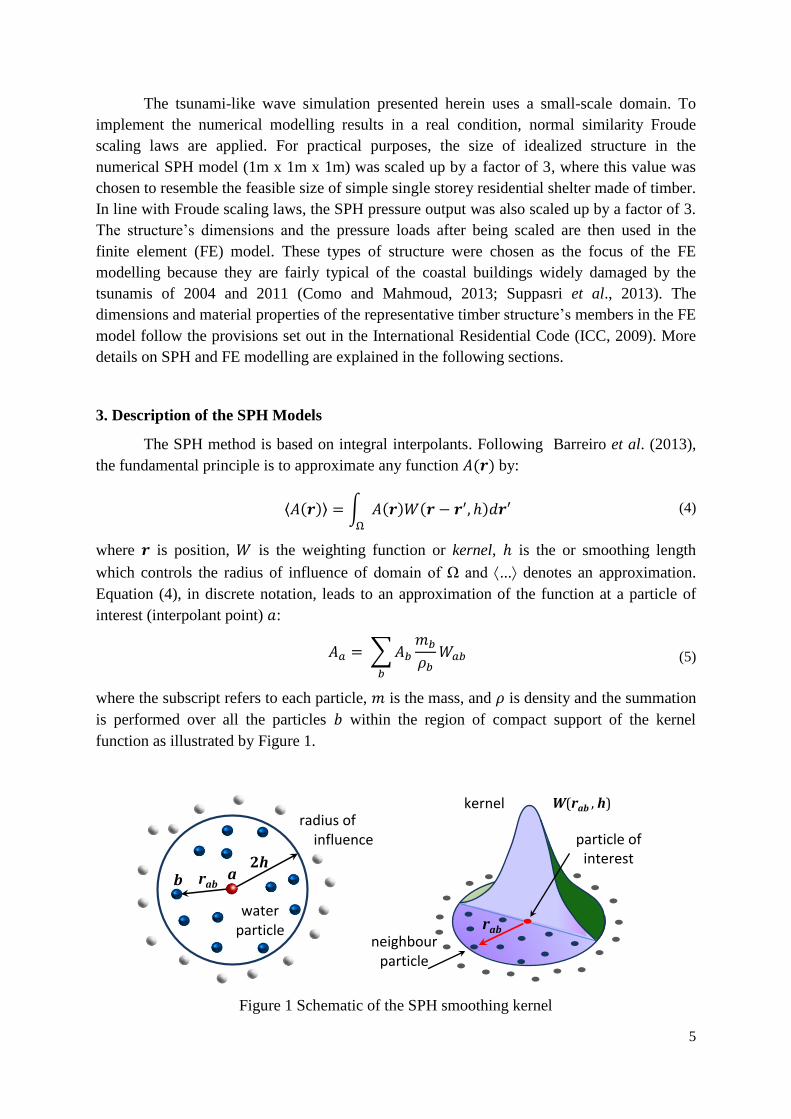
dimension in the associated dambreak model that was used as a reference was the height of

the impact-target structure in the form of a box equal to 0.161 m (see Figure 2a). The height

of the box is denoted herein by L. The convergence study for the pressure predicted at P1 is

depicted in Figure 2b where three different values of 𝑑𝑝 are compared. It can be seen that the

𝑑𝑝 value equal to L/20 gives the closest prediction to the experiment results. Using 𝑑𝑝 values

smaller than L/20 shows little improvement and is too computationally expensive to be

implemented. The GPU specification and run-times are given in Table 1. A list of key

constants and execution parameters in the XML input file used in this study are given in

Table 2. The prediction of the smaller 𝑑𝑝 values is not presented here. Following the results

of the convergence study, the diameter of particle (𝑑𝑝) representing fluids and solid parts in

the model domain was set equal to 0.05 m or 1/20 of the still water level (ℎ0) or the height of

structure (D) that was in this case set to be 1 m, this led to 639,698 particles. Other SPH

simulations that can be considered as convergence studies were the modelling of

experimental works by Linton et al. (2013) and Zhang (2009) that can be found in previous

work by the present authors (Cunningham et al., 2014).

9

(a) Box dimension and probes position (b) SPH pressure at probe P1

Figure 2 Dambreak case for SPH validation

Table 1 GPU specification used in the modelling and the run-times

GPU Specifications SPH model details (DualSPHysics v3.0)

GPU type Tesla M2050 Particle size 0.05 m (L/dp = 1/20)

Memory global 2687 Mb Total particle 639,698

Number of cores 488 Time out 0.025

Clock rate 1.15 GHz Total run time 36 minutes

Table 2 Key XML parameters for input into DualSPHysics

Constants Execution parameters

Particle size dp (m) 0.05 m Step algorithm 2 (Symplectic)

Lattice number bound = 2, fluid =1 Kernel 2 (Wendland)

Cfl number 0.2 Visco treatment 1 (artificial)

Coefficient of sound 10 Viscosity 0.1

Eps value 0.25 Shepard step 30

3.2 Description of geometry of the SPH model

Having established the particle size required to capture the pressure history on the

face of an obstacle similar to those being studied, the focus of the article now shifts to

simulating the input of a tsunami-type bore on a structure near the shoreline.

The geometry of the SPH numerical domain is shown in Figure 3 where a notation of

𝐷 is used in the model to represent its characteristic length of 1 m. The size of model

components or lengths in the geometry is given as a multiple of 𝐷, for example, the size of

structure and the depth of still water are 𝐷, the distance of the structure to the shoreline and to

the rear boundary wall are 2𝐷, and the width of water tank and the height of paddle

P1

P2

P3

P4

0.021 m

0.021 m

0.04 m

0.04 m

0.04 m

0.176 m

0.403 m Y

ZX

0.161 m

0.161m

10

wavemaker are 3𝐷. This was intended to non-dimensionalise the analysis results. Figure 3

indicates the direction from where the pressure distribution can be viewed and this is the

viewpoint (shown by the eye symbol) used for the snapshots shown later.

The dimensions of the numerical water tank here are 15 m long, 3 m wide and 5 m

high. The numerical domain consists of a flat offshore region containing water particles, a

sloping sea bed and onshore region where the coastal structure is placed. In a 3-D model, the

boundary line for the sloping bed (before shoreline) could be the location where water

particle penetration occurs. To prevent an occurrence of excessive fluid particles out of the

boundary, a double layer of particles is used for the boundary line by setting the “lattice

number” equal to two. Excessive out-of-boundary fluid particles could reduce the amount of

fluid particles inside the tank and could affect the wave propagation (reduce the water surface

elevation), especially when it undergoes a long propagation. For all models in this study, the

percentage of the out of boundary fluid particles was limited to less than 1 percent of the total

amount of fluid particles involved.

Figure 3 Side and plan view of 3-D model with simple structure (not to scale)

The parameter varied in the simulations is the wave height based on a ratio between

targeted wave height and still water level (𝐻/ℎ0). Three different values of 𝐻/ℎ0 were used:

0.1, 0.3 and 0.5, these provide the respective wave height 10, 30 and 50 cm for ℎ0 equal to 1

m. Those wave heights resulted in bores when reaching onshore and subsequently impacted

the on-shore structure. A rectangular structure was chosen as representative of a coastal

structure and hence impact target. The dimensions of the rectangular structure are 1m x 1m x

1m. The incoming wave was expected to hit the vertical sides of cube that was perpendicular

to the incoming wave direction. The distance of vertical side of the cube was set 2𝐷 (2 m)

from the shoreline.

7 m3 m 5 m

wav

em

ake

r D

2D 2DD

3 mwave direction

639,698 water particles

3D X

Y

wav

emak

er

water particles

X

Z

h0=D

3 m

D = 1 m

D

viewpoint for 3-D structure pressure distributions

origin located shoreline

open top boundary

11

The origin for the numerical models lies within the model domain and located at the

shoreline. Since DualSPHysics is a single precision code, the position of zero axes can

influence the accuracy of measurements of quantities such as pressure. In other words, a

model with the zero axis located somewhere inside the domain performs better than when its

zero-axis position is situated at the end of or much further from the model domain (Longshaw

and Rogers, 2015). Another advantage of the zero axis position inside the domain, at the

shoreline in this model for instance, is the ease of modifying parts of the model at both ends

of the water tank. For example, when it is necessary to adjust the paddle distances from the

shoreline or change the positions of the target structure (together with the measuring probes)

at the opposite end of the water tank, it can be done without changing large parts of the XML

input file.

4. Computing SPH pressures and forces on the structure

The DualSPHysics software provides output in the form of pressure-time history

measured by numerical measuring probes. This pressure value can be used to estimate the

force. As illustrated in Figure 4, the force (𝐹𝑖) at a certain point in a 3-D model can be

determined by multiplying the pressure (𝑃𝑖) with the area (𝐴𝑖) of probe i, see Equation (12).

Hence, the total force (𝐹) acting normal to a surface can be estimated by summing the force

acting on the total number (𝑛) of areas used to represent the object surface, see Equation (13).

𝐹𝑖 = 𝑃𝑖𝐴𝑖 (12)

𝐹 = ∑ 𝐹𝑖 = ∑(𝑃𝑖𝐴𝑖)

𝑛

𝑖

(13)

Figure 4 Arrangement of probes on the face of the obstacle

Numerical measuring probes were placed at several locations inside the model

domain. The pressure probes were evenly distributed on all surfaces of the target structures

shown in Section 6. The spacing of pressure probes on the structure’s surface facing the

incoming waves is 0.1 m or twice the diameter of particles as the interpolation region around

each probe (which is approximately twice the smoothing length or particle size in radius) is

sufficient to capture the peak pressure. For the vertically-arranged measuring pressure probes,

the probes start at a height of 0.05 m from the bed. Probes for measuring wave velocity and

wave height were placed along the longitudinal axis of the tank (see Figure 5).

probe i

Area (Ai )

12

5. SPH Modelling Results and Discussion

5.a. Water surface elevation

Previous validation for the SPH water surface elevation generated by solitary wave

was presented by Cunningham et al. (2014). Here, we present the results for different wave

height to water depth ratios. Figure 5 shows the probe positions for measuring water surface

elevation regarding the propagation of the solitary wave for cases with different H/h0. The

water surface elevations were measured at certain probes along the tank. H1 is placed 1 m

from shoreline and followed by H2 through H7 at a constant 1 m spacing apart. The

properties of the offshore solitary waves and onshore bores can be seen from Figure 6 and

Figure 7 and also from Table 3.

Figure 5 Layout of water surface elevation probes H1-H7

Figure 6 depicts the SPH simulation of the solitary wave propagation offshore for the

case with 𝐻/ℎ0 = 0.5. From the four snapshots given in Figure 6a to Figure 6d, the changes

in the solitary wave profile/shape can be observed. Near the shoreline at probe H1, the

solitary wave started to break and its elevation decreased as illustrated in more detail in

Figure 7.

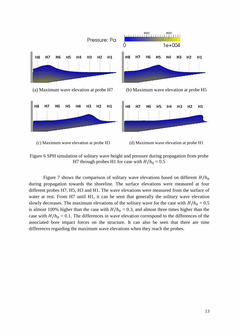
13

(a) Maximum wave elevation at probe H7 (b) Maximum wave elevation at probe H5

(c) Maximum wave elevation at probe H3 (d) Maximum wave elevation at probe H1

Figure 6 SPH simulation of solitary wave height and pressure during propagation from probe

H7 through probes H1 for case with 𝐻/ℎ0 = 0.5

Figure 7 shows the comparison of solitary wave elevations based on different 𝐻/ℎ0

during propagation towards the shoreline. The surface elevations were measured at four

different probes H7, H5, H3 and H1. The wave elevations were measured from the surface of

water at rest. From H7 until H1, it can be seen that generally the solitary wave elevation

slowly decreases. The maximum elevations of the solitary wave for the case with 𝐻/ℎ0 = 0.5

is almost 100% higher than the case with 𝐻/ℎ0 = 0.3, and almost three times higher than the

case with 𝐻/ℎ0 = 0.1. The differences in wave elevation correspond to the differences of the

associated bore impact forces on the structure. It can also be seen that there are time

differences regarding the maximum wave elevations when they reach the probes.

14

(a) Probe H7 (b) Probe H5

(c) Probe H3

(d) Probe H1

Figure 7 Comparison of solitary wave elevations for different 𝐻/ℎ0 measured at probe H7,

H5, H3 and H1.

5.b. Bore Height and Velocity

The onshore bore heights and velocities were measured by probes placed in front of

the structure. The values of these properties are important in determining the exerted pressure

on the surface of structure. The snapshots of the bores including velocities can be seen in

Figure 8 and the variation of bore heights are depicted in Figure 9, for simulation cases with

H/h0 = 0.3 and 0.5.

-0.1

0

0.1

0.2

0.3

0.4

0.5

0.6

0.7

0.8

0 2 4 6 8 10

Ele

vati

on

: m

Time: s

/ℎ₀ = 0.5 /ℎ₀ = 0.3 /ℎ₀ = 0.1

-0.1

0

0.1

0.2

0.3

0.4

0.5

0.6

0.7

0.8

0 2 4 6 8 10

Ele

vati

on

: m

Time: s

/ℎ₀ = 0.5 /ℎ₀ = 0.3 /ℎ₀ = 0.1

-0.1

0

0.1

0.2

0.3

0.4

0.5

0.6

0.7

0.8

0 2 4 6 8 10

Ele

vati

on

: m

Time: s

/ℎ₀ = 0.5 /ℎ₀ = 0.3 /ℎ₀ = 0.1

-0.1

0

0.1

0.2

0.3

0.4

0.5

0.6

0.7

0.8

0 2 4 6 8 10

Ele

vati

on

: m

Time: s

/ℎ₀ = 0.5 /ℎ₀ = 0.3 /ℎ₀ = 0.1

15

(a) (b)

Figure 8 SPH simulation of bore velocity for the case with 𝐻/ℎ0 = 0.5: (a) near the shoreline

and (b) onshore.

(a) Shoreline (b) Onshore

Figure 9 Bore height measured from still water level at (a) shoreline, (b) onshore.

Table 3 shows the offshore water surface elevation and wave length of solitary waves

and the corresponding onshore bore characteristics (height and velocity). It can be observed

that offshore, the maximum velocity increases proportionally with the design height of the

solitary wave, but inversely proportional to the wave length of the wave. The maximum

solitary wave velocities offshore are also proportional to the bore height and velocity

onshore.

-0.1

0

0.1

0.2

0.3

0.4

0.5

0.6

0.7

0.8

0 2 4 6 8 10

Ele

vati

on

: m

Time: s

/ℎ₀ = 0.5 /ℎ₀ = 0.3 /ℎ₀ = 0.1

-0.1

0

0.1

0.2

0.3

0.4

0.5

0.6

0.7

0.8

0 2 4 6 8 10

Ele

vati

on

: m

Time: s

/ℎ₀ = 0.5 /ℎ₀ = 0.3 /ℎ₀ = 0.1

16

Table 3 Solitary wave and bore properties

𝐻/ℎ0 Offshore solitary waves Onshore bores

Maximum

elevation

Maximum

velocity

Wave

length

Maximum

height

Maximum

velocity

0.5 0.7 m 3.94 m/s 5.0 m 0.32 m 5.65 m/s

0.3 0.4 m 2.13 m/s 6.5 m 0.20 m 4.05 m/s

0.1 0.15 m 0.68 m/s 7.7 m 0.11 m 1.19 m/s

5.c. Wave Pressure

Typical output from the 3-D SPH simulation is shown in Figure 10 and Figure 11 for

the case with H/h0 = 0.5. Figure 10a depicts the snapshot of a propagating solitary wave

which is then followed by a bore impact on the structure as shown by Figure 10b. The peak

pressure impact occurred at t = 4.150 sec and the peak pressure took place at the lowest level

of pressure probes as indicated by the circle in the Figure 10a. In addition, Figure 11b shows

the pressure distribution for the maximum bore run-up on the surface of the structure that

occurred at t = 4.325 sec and corresponding with Figure 10b. Pressure distributions in Figure

11 were seen from the rear of the structure (see illustration indicating direction of view in

Figure 3) by assuming the cube structure is visually transparent.

17

(a) (b)

Figure 10 Oblique view of the 3-D simulation for case H/h0 = 0.5; (a) solitary wave

propagation at t = 3.150 sec. (related with Figure 6c), (b) bore impacting structure at t = 4.325

sec.

(a) (b)

Figure 11 Pressure distribution on vertical surface at H/h0 = 0.5; (a) first impact at t = 4.150

sec, (b) peak impact occurred at the circled probe at t = 4.325 sec.

The normalised peak pressures (𝑃/𝜌𝑔ℎ0) for the simulation with H/h0 = 0.1, 0.3 and

0.5 were 0.748, 18.165 and 83.287, respectively. The bore pressures for the case with H/h0 =

0.1 were comparatively small and resulted in a correspondingly small impact force. Hence,

the comparison of the predicted impact pressure between the numerical and the empirical

equation were made only for the case with H/h0 = 0.3 and 0.5. The numerical maximum

pressure for the case with wave height equal to H/h0 = 0.3 and 0.5 were 10,508 N/m2, and

37,371 N/m2, respectively. The associated pressures determined by Equation (2) were 1,766

N/m2 and 4,520 N/m

2 over the bore height for the case with H/h0 = 0.3 and 0.5, respectively.

In addition, the impact pressures predicted by Equation (3) were 3532 N/m2 and 5651 N/m

2

over the bore height for the case with H/h0 = 0.3 and 0.5, respectively. However, these results

must be viewed within the context that in general the design equations adopt a quasi-static

approach to wave pressures, whereas in reality the peak pressure occurs over a very short

time period and may be very localised.

peak impact location

18

6. Finite Element Modelling

The finite element modelling was conducted to study the behaviour of a simple

dwelling type structure made of timber under tsunami-like wave bore impact loading. The

response of the structures, especially the stress distribution on the main load-bearing

components i.e. the vertical studs, will be compared with the behaviour resulting from the

quasi-static pressure given by Equation (2).

The dynamic analysis was performed using ABAQUS Explicit (ABAQUS, 2010). In

this procedure the equations of motion are integrated in time explicitly using central

difference integration rules. The analysis procedure requires a small time increment and since

it does not need to solve a global set of equations in each increment, the computational cost

per increment is relatively small compared with the implicit method. The explicit method is

well suited to modelling short duration/transient loads such as those associated with tsunami

wave impacts.

6.1 Model Properties

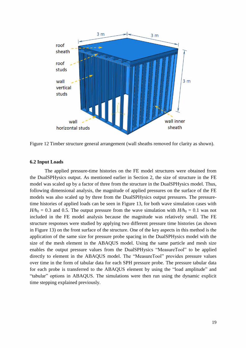
Figure 12 shows a definition sketch of the timber structure. As previously stated, the

structure dimensions for the FE model are 3m x 3m x 3m. The target structure consists of

four vertical walls and a flat roof all composed of sandwich timber panels. The sandwich

panel is an arrangement of sheath-stud-sheath. The sheath is made of plywood with 13 mm

thickness and has the following material properties: density = 750 kg/m3, Young’s modulus =

7.7x109 N/m

2 and Poisson’s ratio = 0.22. The studs are made of softwood timber (Douglas

fir) with a cross sectional size of 38 mm wide x 140 mm deep and installed with spacing

centres of 420 mm. The studs’ material properties are as follows: density = 530 kg/m3,

Young’s modulus = 7.0x109 N/m

2 and Poisson’s ratio = 0.22. The timber structure was

designed to be simply supported at the base i.e. no rotational fixity. The timber structure

components were modelled using 8-node linear brick elements (type C3D8R) with reduced-

integration and hour-glass control.

19

Figure 12 Timber structure general arrangement (wall sheaths removed for clarity as shown).

6.2 Input Loads

The applied pressure-time histories on the FE model structures were obtained from

the DualSPHysics output. As mentioned earlier in Section 2, the size of structure in the FE

model was scaled up by a factor of three from the structure in the DualSPHysics model. Thus,

following dimensional analysis, the magnitude of applied pressures on the surface of the FE

models was also scaled up by three from the DualSPHysics output pressures. The pressure-

time histories of applied loads can be seen in Figure 13, for both wave simulation cases with

H/h0 = 0.3 and 0.5. The output pressure from the wave simulation with H/h0 = 0.1 was not

included in the FE model analysis because the magnitude was relatively small. The FE

structure responses were studied by applying two different pressure time histories (as shown

in Figure 13) on the front surface of the structure. One of the key aspects in this method is the

application of the same size for pressure probe spacing in the DualSPHysics model with the

size of the mesh element in the ABAQUS model. Using the same particle and mesh size

enables the output pressure values from the DualSPHysics “MeasureTool” to be applied

directly to element in the ABAQUS model. The “MeasureTool” provides pressure values

over time in the form of tabular data for each SPH pressure probe. The pressure tabular data

for each probe is transferred to the ABAQUS element by using the “load amplitude” and

“tabular” options in ABAQUS. The simulations were then run using the dynamic explicit

time stepping explained previously.

20

(a) 𝐻/ℎ0 = 0.3 (b) 𝐻/ℎ0 = 0.5

Figure 13 Applied pressure time histories for the finite element models.

The pressures applied on the vertical surface of the structures were divided into 10

layers. This number of layers was identical with the number of probes arranged vertically in

the SPH model, denoted by Lp in Figure 13. The magnitude of pressure at each layer is the

average pressure measured by pressure probes at the associated layer. The reason for

applying average pressure history at each layer was based on time efficiency. Also, it was

found that the pressure variation measured by SPH probes within the same layer is generally

not significant. Figure 13(a) shows the applied loads presented from Layer 1 to Layer 7 (Lp1

to Lp7). Loads at Layer 8 to Layer 10 (Lp8 to Lp10) are zero so they were not included in the

graph. In Figure 13(b) all 10 layers were loaded. The loaded layers on the surface were

related with the height of bore runup on the surface of the wall.

The negative pressure values in Figure 13 reflect the application of the equation of

state in DualSPHysics and a rebound or suction effect. DualSPHysics version 3.0 is still a

single phase model that cannot yet perform multiphase behaviour including air and water at

the same time. The next version of DualSPHysics (version 4.0) is being developed to be

capable of performing such multi-phase modelling (Mokos et al., 2015). Two peaks are

shown in the pressure-time histories in Figure 13. The first peak occurred when the leading

edge of the bore impacted the structure and the second peak occurred when the splashing

followed with the main flow. These two peak phenomena are typical for impact loads of this

type and were also observed in the experiment by Fujima et al. (2009). Note in the case of the

immediate impact on the structure, no additional force is applied e.g. drag force. The

hydrodynamic ‘drag’ forces indeed occur in real tsunami events (Yeh et al., 2014) and affect

the structure when surrounded by a ‘steady’ fluid flow with relatively constant velocity

(FEMA, 2011). However in this simulation, the hydrodynamic drag was not so significant

-20

0

20

40

60

80

100

120

0 2 4 6 8 10

Pre

ssu

re: k

Pa

Time: sec

7

6

5

4

3

2

1

-20

0

20

40

60

80

100

120

0 2 4 6 8 10

Pre

ssu

re: k

Pa

Time: sec

10

9

8

7

6

5

4

3

2

1

21

(see Figure 14) because of the application of a single stroke solitary wave where the most

dominant effect was the highly transient impulsive pressure immediately following the

impact of the leading edge of the arriving water mass.

Figure 14 Plan view of SPH simulation showing no significant drag force on the sides

of structure.

6.3 Analysis and Results

The finite element analysis was performed using the ABAQUS Dynamic Explicit

module with duration of simulation of 2.6 seconds and time increment automatically

determined by the program. The duration of simulation was enough to capture the important

segment of pressure-time histories given in Figure 13 incorporating the peak impact and

subsequent impact. All components of the structure were meshed with the finest mesh on the

front surface. The size of the mesh for the front impacted surface was 0.05 m to correspond

with the diameter of SPH fluid particles, a coarser mesh with twice the size of elements was

used for the other sides of the structure. The response of the structures is shown in terms of

the maximum principal stress that occurred on the members. On the front face of the

structure, the main load carrying elements are the vertical and horizontal studs and these are

shown in Figure 15 by removing the outer plywood cover sheath.

The results of the finite element modelling can be seen in Figure 15 which consists of

five figures showing the response of the structure under different loading conditions. Figure

15(a) and Figure 15(b) shows the response of structures loaded by the SPH pressure time-

history resulting from a normalised wave height H/h0 = 0.3 and 0.5, respectively. Figure 15c

and Figure 15(d) on the other hand show the response of the structure under a quasi-static

pressure determined using the semi-empirical approach given by Equation (2) using the

equivalent wave properties. The pressures related with Figure 15(c) and Figure 15(d) were

calculated based on a bore height of 0.60 m and 0.96 m, respectively, where those bore

heights were taken from the SPH model simulation (see Table 3) and scaled-up by a factor of

3. The application of those bore heights in Equation (2) was intended to accomplish

straightforward comparison of the structure’s response based on numerical and semi-

empirical approaches.

22

(a) SPH-based pressure (case H/h0 = 0.3) (b) SPH-based pressure (case H/h0 = 0.5)

(c) Quasi static-based pressure (case H/h0 = 0.3) (d) Quasi static-based pressure (case H/h0 = 0.5)

(e) Close up view of area of maximum stress indicated in Figure 15(b).

Figure 15 FE Dynamic response due to SPH pressure-time history (a, b); FE static response

due to quasi-static pressure from Equation (2) (c, d); location of maximum stresses (e); (all

stresses shown in N/m2).

observed

area

in Figure (e)

23

Figure 15(a) and Figure 15(b) show that the maximum principal stresses occurred at

the tension side, below the mid-span of the vertical studs. The stresses shown in Figure 15(a)

and Figure 15(b) are the maximum stresses that occurred at any time in the response to the

bore impact and not necessarily simultaneous with the maximum impact pressure. In the case

of Figure 15(b), the stresses are approaching the flexural capacity for this type of timber. This

general type of flexural failure is in line with experimental results reported by (Lacroix and

Doudak, 2014) whereby the vertical studs on timber panels failed due to the out of plane

high strain rate induced by blast loading, while in this case the tsunami impact load could

also be categorized a high strain rate event as indicated by the pressure time histories in

Figure 13. For comparable scale structures, similar failure patterns of timber studs in flexure

due to tsunami-like wave impact was reported experimentally by Linton et al. (2013). It can

also be seen that under higher loads (Figure 15b) the stress concentration tends to develop

closer to the lower end of the studs in comparison with Figure 15(a). In this case, a shear-type

failure of the stud would be expected. Figure 15(c) and Figure 15(d) show the response of the

structure under the static loads resulting from Equation (2). It can be seen that the maximum

stresses concentrated at the bottom end of the vertical studs. This response is due to load

being applied on the lower part of the structure over the height of the bore. In both Figure

15(c) and Figure 15(d) it should be noted that the predicted quasi-static pressures resulted in

timber stresses at least 4 times less than those observed in the dynamic response using the

SPH derived pressure-time histories. In real terms, these values represent the difference

between the focussed structure remaining intact or not.

7. Conclusions

In this paper, the interactions between a tsunami bore and an idealized timber

structure were modelled using the SPH based software DualSPHysics coupled with finite

element analysis using ABAQUS. The SPH models show the ability of this approach to

provide impact pressure distributions in a great level of detail both spatially and temporally.

The results from the SPH models were utilized in the finite element model to predict the

response of the structure under transient bore impact loads. The numerical pressure

predictions were also compared with pressure predictions from semi-empirical approaches

used in design codes. The structure response results highlight the potential for non-

conservatisms in the empirical approaches. The techniques outlined in this paper can allow

engineers to gain a better insight into tsunami wave-structure interaction and thus lead to

resilience optimisation of structures vulnerable to these type of events. Further development

is needed for more complex tsunami-like bore and structure interactions including the effect

of aeration via multi-phase SPH wave modelling.

8. Acknowledgements

The authors gratefully acknowledge the contribution of the Directorate General of Higher

Education of The Republic of Indonesia to the funding of this research. Support from

24

Warmadewa University of Bali, Indonesia, is also appreciated. Thanks are due to Dr

Athanasios Mokos for his assistance with DualSPHysics modelling.

25

References

ABAQUS. (2010). ABAQUS analysis user’s manual. Providence, Rhode Island, USA.,

SIMULIA, Dassault Systèmes.

Altomare, C., Crespo, A. J. C., Domínguez, J. M., Gómez-Gesteira, M., Suzuki, T., &

Verwaest, T. (2015). Applicability of Smoothed Particle Hydrodynamics for estimation

of sea wave impact on coastal structures. Coastal Engineering, 96, 1–12.

Barreiro, A., Crespo, A. J. C., Domínguez, J. M., & Gómez-Gesteira, M. (2013). Smoothed

Particle Hydrodynamics for coastal engineering problems. Computers & Structures, 120,

96–106.

Becker, A. B., Johnstone, W. M., & Lence, B. J. (2011). Wood frame building response to

rapid-onset flooding. Natural Hazards Review, 12(2), 85–95.

Camfield, F. (1980). Tsunami engineering. Special Report SR-6. Coastal Engineering

Research Center, U.S. Army Corps of Engineers, Springfield, VA.

Canelas, R., Ferreira, R. M. L., Crespo, A. J. C., & Domínguez, J. M. (2013). A generalized

SPH-DEM discretization for the modelling of complex multiphasic free surface flows.

In Proceedings of the 8th International SPHERIC Workshop (p. 6). Trondheim, Norway.

CCH. (2000). City and County of Honolulu Building Code (CCH). Chapter 16, Article 11.

Department of Planning and Permitting of Honolulu Hawaii, Honolulu, HI.

Chanson, H. (2006). Tsunami Surges on Dry Coastal Plains: Application of Dam Break Wave

Equations. Coastal Engineering Journal, 48(04), 355–370.

http://doi.org/10.1142/S0578563406001477

Como, A., & Mahmoud, H. (2013). Numerical evaluation of tsunami debris impact loading

on wooden structural walls. Engineering Structures, 56, 1249–1261. Retrieved from

http://dx.doi.org/10.1016/j.engstruct.2013.06.023.

Crespo, A. J. C., Dominguez, J. M., Barreiro, A., Gómez-Gesteira, M., & Rogers, B. D.

(2011). GPUs, a new tool of acceleration in CFD: Efficiency and reliability on smoothed

particle hydrodynamics methods. PLoS ONE, 6(6).

Crespo, A. J. C., Dominguez, J. M., Gesteira, M. G., Barreiro, A., Rogers, B. D., Longshaw,

S., … Vacondio, R. (2013). User Guide for DualSPHysics code v3.0.

Crespo, A. J. C., Domínguez, J. M., Rogers, B. D., Gómez-Gesteira, M., Longshaw, S.,

Canelas, R., … García-Feal, O. (2015). DualSPHysics: Open-source parallel CFD solver

based on Smoothed Particle Hydrodynamics (SPH). Computer Physics Communications,

187, 204–216.

Crespo, A. J. C., Gomez-Gesteira, M., & Dalrymple, R. A. (2007). Boundary conditions

generated by dynamic particles in SPH methods. Cmc-Computers Materials &

Continua, 5, 173–184.

Cunningham, L. S., Rogers, B. D., & Pringgana, G. (2014). Tsunami wave and structure

interaction: an investigation with smoothed-particle hydrodynamics. ICE Journal of

Engineering and Computational Mechanics, 167(EM3), 126–138.

Dalrymple, R. A., Gómez-Gesteira, M., Rogers, B. D., Panizzo, A., Zou, S., Crespo, A. J. C.,

… Narayanaswamy, M. (2009). Smoothed particle hydrodynamics for water waves. in

Advances in numerical simulation of nonlinear water waves, ed. Ma, Q., Singapore:

World Scientific Publishing.

Dames and Moore. (1980). Design and construction standards for residential construction in

26

tsunami prone areas in Hawaii. Federal Emergency Management Agency, Washington,

D.C.

Farahani, R. J., Dalrymple, R. A., Hérault, A., & Bilotta, G. (2014). Three-dimensional SPH

modeling of a bar/rip channel system. Journal of Waterway, Port, Coastal, and Ocean

Engineering, 140(1), 82–99.

FEMA. (2003). Coastal Construction Manual. (3 vols.) 3rd ed. (FEMA 55). Federal

Emergency Management Agency, Jessup, MD.

FEMA (Federal Emergency Management Agency). (2011). Coastal Construction Manual.

FEMA P-55 (Vol. II). Washington, DC, USA.

Fujima, K., Achmad, F., Shigihara, Y., & Mizutani, N. (2009). A Study on Estimation of

Tsunami Force Acting on Structures. Journal of Disaster Research, 4(6), 404–409.

Gomez-Gesteira, M., Crespo, A. J. C., Rogers, B. D., Dalrymple, R. A., Dominguez, J. M., &

Barreiro, A. (2012). SPHysics - development of a free-surface fluid solver - Part 2:

Efficiency and test cases. Computers and Geosciences, 48(2), 300–307.

Gomez-Gesteira, M., Rogers, B. D., Crespo, A. J. C., Dalrymple, R. A., Narayanaswamy, M.,

& Dominguez, J. M. (2012). SPHysics – development of a free-surface fluid solver –

Part 1: Theory and formulations. Computers & Geosciences, 48(1), 289–299.

International Code Council. (2009). 2009 International residential code for one- and two-

family dwellings. Country Club Hills, IL.

IOC (Intergovernmental Oceanographic Commission). (2013). Tsunami Glossary (Revised

Ed). UNESCO, IOC Technical Series, 85, Paris: United Nations Educational, Scientific

and Cultural Organization.

Kleefsman, K. M. T., Fekken, G., Veldman, A. E. P., Iwanowski, B., & Buchner, B. (2005).

A Volume-of-Fluid based simulation method for wave impact problems. Journal of

Computational Physics, 206, 363–393.

Lacroix, D. N., & Doudak, G. (2014). Investigation of Dynamic Increase Factors in Light-

Frame Wood Stud Walls Subjected to Out-of-Plane Blast Loading. Journal of Structural

Engineering, ASCE, 1–10.

Lind, S. J., Xu, R., Stansby, P. K., & Rogers, B. D. (2012). Incompressible smoothed particle

hydrodynamics for free-surface flows: A generalised diffusion-based algorithm for

stability and validations for impulsive flows and propagating waves. Journal of

Computational Physics, 231(4), 1499–1523.

Linton, D., Gupta, R., Cox, D., van de Lindt, J., Oshnack, M. E., & Clauson, M. (2013).

Evaluation of Tsunami Loads on Wood Frame Walls at Full Scale. Journal of Structural

Engineering, 139(8), 1318–1325.

Longshaw, S. M., & Rogers, B. D. (2015). Automotive fuel cell sloshing under temporally

and spatially varying high acceleration using GPU-based Smoothed Particle

Hydrodynamics (SPH). Advances in Engineering Software, 83, 31–44.

McCabe, M., Stansby, P. K., Rogers, B. D., & Cunningham, L. S. (2014). Boussinesq

modelling of tsunami and storm wave impact. ICE Journal of Engineering and

Computational Mechanics, 167(EM3), 106–116.

Mokos, A., Rogers, B. D., Stansby, P. K., & Domínguez, J. M. (2015). Multi-phase SPH

modelling of violent hydrodynamics on GPUs. Computer Physics Communications, 196,

304–316.

27

Monaghan, J. J. (1992). Smoothed particle hydrodynamics. Ann. Rev. Astron. Astrophys., 30,

543–574.

Nouri, Y., Nistor, I., Palermo, D., & Cornett, A. (2010). Experimental Investigation of

Tsunami Impact on Free Standing Structures. Coastal Engineering Journal, 52(01), 43–

70.

Okada, T., Sugano, T., Ishikawa, T., Ohgi, T., Takai, S., & Hamabe, C. (2005). Structural

design methods of buildings for tsunami resistance (SMBTR). The Building Center of

Japan, Japan.

Palermo, D., Nistor, I., Nouri, Y., & Cornett, A. (2009). Tsunami loading of near-shoreline

structures: a primer. Canadian Journal of Civil Engineering, 36(11), 1804–1815.

http://doi.org/10.1139/L09-104.

Robertson, I. N., Riggs, H. R., Paczkowski, K., & Mohamed, A. (2011). Tsunami bore forces

on walls. In Proceedings of the ASME 2011, 30th International Conference on Ocean,

Offshore and Arctic Engineering (pp. 1–9). Rotterdam, The Netherlands.

St-Germain, P., Nistor, I., Townsend, R., & Shibayama, T. (2014). Smoothed-Particle

Hydrodynamics Numerical Modeling of Structures Impacted by Tsunami Bores. Journal

of Waterway, Port, Coastal, and Ocean Engineering, 140(1), 66–81.

Suppasri, A., Shuto, N., Imamura, F., Koshimura, S., Mas, E., & Yalciner, A. C. (2013).

Lessons Learned from the 2011 Great East Japan Tsunami: Performance of Tsunami

Countermeasures, Coastal Buildings, and Tsunami Evacuation in Japan. Pure and

Applied Geophysics, 170(6), 993–1018.

Violeau, D., & Rogers, B. D. (2016). Smoothed particle hydrodynamics (SPH) for free-

surface flows: past, present and future. Journal of Hydraulic Research, 54(1), 1–26.

Yeh, H., Barbosa, A. R., Ko, H., & Cawley, J. (2014). Tsunami Loadings on Structures.

Coastal Engineering, 1–13.

Zhang, W. (2009). An Experimental Study and A Three-Dimensional Numerical Wave Basin

Model of Solitary Wave Impact on A Vertical Cylinder. School of Civil and Construction

Engineering. Oregon State University.

28

Notations

𝐴𝑖 tributary area where pressure probe i is situated (m2)

a particle a

B the breadth of structure (m)

b particle b

𝐷 represent a certain length of 1 m in the SPH model

𝐷𝐹 the distance of structure from shoreline (m)

𝑑𝑝 water particle size or the initial spacing of particle (m)

E Young’s modulus of elasticity (m kg s-2

)

𝐹𝑖 force at a certain point in a 3-D model (kg m s-2

)

g gravitational acceleration (m s-2

)

H solitary wave height (m)

h characteristic smoothing length (m)

h0 offshore water depth/still water level (m)

ℎ𝑏 the height of the bore (m)

him maximum inundation depth (m)

L shortest dimension of box in convergence study (m)

𝐿𝑝 the layers of pressure probes

m mass of SPH particle (kg)

𝑃𝑖 pressure at a certain area in a 3-D model (kg m-1

s-2

)

rab distance between two particles (m)

ρ density, density of SPH particle (kg m-3

)

𝑣 Poisson’s ratio

𝑣𝑗 the velocity of bore (m s-1

)

W weighting function or kernel

𝜞 dissipative term

𝜫𝑎𝑏 viscosity term