modelling of the effect of grain boundary diffusion on the
TRANSCRIPT

HAL Id: cea-01818751https://hal-cea.archives-ouvertes.fr/cea-01818751
Submitted on 14 Jan 2019
HAL is a multi-disciplinary open accessarchive for the deposit and dissemination of sci-entific research documents, whether they are pub-lished or not. The documents may come fromteaching and research institutions in France orabroad, or from public or private research centers.
L’archive ouverte pluridisciplinaire HAL, estdestinée au dépôt et à la diffusion de documentsscientifiques de niveau recherche, publiés ou non,émanant des établissements d’enseignement et derecherche français ou étrangers, des laboratoirespublics ou privés.
Modelling of the effect of grain boundary diffusion onthe oxidation of Ni-Cr alloys at high temperatureLéa Bataillou, Clara Desgranges, Laure Martinelli, Daniel Monceau
To cite this version:Léa Bataillou, Clara Desgranges, Laure Martinelli, Daniel Monceau. Modelling of the effect of grainboundary diffusion on the oxidation of Ni-Cr alloys at high temperature. Corrosion Science, Elsevier,2018, 136, pp.148-160. �10.1016/j.corsci.2018.03.001�. �cea-01818751�

Modelling of the effect of grain boundary diffusion on the oxidation of Ni-Cr alloys at high temperature
Léa Batailloua,c,⁎, Clara Desgrangesa,b, Laure Martinellia, Daniel Monceauc
a Den-Service de la Corrosion et du Comportement des Matériaux dans leur Environnement (SCCME), CEA, Université Paris-Saclay, F-91191, Gif-sur-Yvette, Franceb Safran-Tech, rue des jeunes bois, Châteaufort, CS 80112, 78772 Magny les hameaux, Francec CIRIMAT, Université de Toulouse, CNRS, INPT, UPS, 4 allée Emile Monso, BP 44362, 33103 Toulouse Cedex 4, France
Grain boundaries in oxide scales have a strong effect on oxidation kinetics when they act as diffusion shortcircuits. This study proposes a quantitative evaluation of the phenomenon by modelling. Various cases of oxidemicrostructure evolution are treated using both analytical and numerical resolutions. Results showed that theeffect of oxide grain growth on the oxidation kinetics can be analysed considering a transitory stage for whichthe oxidation kinetics is not purely parabolic. Some guidelines for choosing the appropriate post-treatmentmethod for the analysis and extrapolation of experimental oxidation kinetics are given.
1. Introduction
Parabolic constants values reported in literature for chromiaforming alloys [1–13] are distributed on several orders of magnitude,these values are gathered on Fig. 1. It has been shown that under O2
atmospheres, chromia grow by diffusion of spieces across the oxidescale [13,15,16] and that diffusion short-circuits, such as grainboundaries in oxide scales, have a major effect on oxidation kinetics[10,17,18].
In his review on the influence of grain boundary diffusion on hightemperature oxidation, Atkinson [1] showed that the values of the ex-perimental parabolic constant (kp) published for chromia are dis-tributed over a range of about three orders of magnitude for the sametemperature. Atkinson calculated theoretical kp values for polycristal-line chromia using tracer diffusion coefficient from Hagel et al. [14],and kp value for single cristal chromia using single cristal tracer diffu-sion coefficient for chromia that he determined experimentally [1]. Heshowed that experimental reported kp values were closer to theoreticalvalues corresponding to polycrystalline chromia than to theoreticalvalue corresponding to single crystal chromia. These experimental andtheoretical kp values are plotted on Fig. 1. Knowing that the calculatedkp for polycrystalline chromia can be up to six orders of magnitudehigher than the one of single crystal chromia, it was concluded thatchromia growth was quantitatively affected by grain boundary diffu-sion [1]. Notice that such a dispersion of reported kp values can also be
explained by other phenomena such as a transitory regime caused byformation of NiO [19] or the presence of reactive elements that canslow down diffusion [10,20].
Concerning the influence of grain boundaries, several authors pro-posed oxidation models taking into account accelerated diffusion byshort-circuit diffusion paths. Perrow et al. [18] proposed an analyticalsolution for oxidation kinetics taking into account grain boundary dif-fusion in nickel oxide scales. They used the effective diffusion coeffi-cient proposed by Hart [21], which is a weighted average betweenlattice and short-circuit diffusion coefficients. Hart’s law was initiallyestablished for the modelling of accelerated diffusion by dislocation.However, it can be adapted to diffusion through grain boundaries.Besides the use of Hart’s law, Perrow et al. [18] added the influence ofgrain size evolution via a parabolic growth law. Hussey et al. [22], whoworked on iron oxides growth kinetics, followed the same hypothesesas Perrow et al. [18] and determined an instantaneous parabolic rateconstant in the case of a parabolic oxide grain growth. Rhines et al.[23,24] observed cubic oxidation kinetics on NiO scales associated witha cubic grain size growth. Davies and Smeltzer [25,26] proposed ananalytical treatment by means of an exponential law for the decay ofshort-circuit proportion over time. More recently, Hallström et al. [27]proposed a numerical approach based on thermodynamics calculationsapplied to chromia growth. Nevertheless, this model does not takeoxide microstructure evolution into account. Other authors have con-sidered the diffusion through grain boundaries in oxide scales [28–30]
⁎ Corresponding author at: Den-Service de la Corrosion et du Comportement des Matériaux dans leur Environnement (SCCME), CEA, Université Paris-Saclay, Gif-sur-Yvette, F-91191,France.
E-mail addresses: [email protected] (L. Bataillou), [email protected] (C. Desgranges), [email protected] (L. Martinelli),[email protected] (D. Monceau).
1

and even the influence of oxide microstructure on oxidation kinetics[31,32], with an experimental approach.
Some different approaches have been developed concerning oxida-tion kinetics modelling by taking into account formation and growth ofseveral phases which are also steps forward the description of complexoxide microstructure. Larsson et al. [33] performed a numerical simu-lation of multiphasic iron oxide growth. Nijdam et al. [34,35] devel-oped coupled thermodynamic-kinetics oxidation model, which is ableto predict the phases formed and their impact on oxidation kinetics.
In this framework, this study proposes a new quantitative estima-tion of the influence of grain boundary diffusion on oxidation kinetics.Oxidation models proposed are applied on chromia-forming alloys. Thestudied cases consider (1) the evolution of grain size over time, (2) agrain size gradient across the oxide scale, and (3) a combination ofboth. For the simplest cases (1) and (2), some new analytical solutionswere found. However, for the complex cases (3), which combine grainsize evolution in time and space, a numerical approach is required. Thenumerical EKINOX model [36–38] has been used and modified for thisstudy in order to take into account grain boundary diffusion and mi-crostructural evolutions in the oxide scale. Chromia growth kineticswere then modelled using input data based on literature experimentaldata [10].
The first part of this paper presents the existing oxidation kineticsmodels available in the literature. These models take into account bothlattice and grain boundary diffusion in the oxide scale according to A-type diffusion [39] and consider homogeneous oxide grain size orsimple grain size growth law. The second part is dedicated to newanalytical models proposed, and to the numerical modelling using theEKINOX code. These new models are able to take into account the oxidegrain size growth according to a cubic law and a grain size gradientacross the oxide scale. Moreover, a numerical model is adapted in orderto treat the complex case of grain size growth and grain size gradientcombination.
In results section kinetics obtained using the various analytical andnumerical models are presented. Firstly, these oxidation kinetics are
discussed, and then, a parametric study is carried out on the effects ofthe oxide grain size growth kinetics. In the discussion part, the twomethods, which are usually performed for the analysis and the extra-polation of experimental oxidation kinetics, are used on calculated ki-netics and they are compared. These are referred in this work as the“parabolic law” method and the “log-log” method. Finally, the twomethods are compared for long term extrapolation.
2. Literature models for oxidation kinetics and extrapolationmethods
2.1. Wagner’s theory simplified
In the case of continuous oxide scale formation, Wagner proposes amodel for oxide scale growth that looks at diffusion across the oxidescale as the rate-limiting step [40]. A simplified expression for theparabolic rate constant can be given assuming that the species con-centrations at metal/oxide and oxide/gas interfaces are time invariant.This assumption supposes that diffusion occurs through lattice only,that the diffusion coefficient is constant and that usual hypotheses ofstationarity, electroneutrality and fluxes conservation are assumed[40]:
= − +e k t t e( )2p,L 0 0
2 (1)
= ∼k ΩD C2 Δp,L L (2)
2.2. Diffusion models taking into account bulk and short-circuit diffusion
When the influence of diffusion along short circuits is taken intoaccount within the global diffusion phenomenon, several limiting casescan be described. These different cases depend on the space distributionof grain size and on the values of diffusion coefficients in lattice and inshort circuits [41,42]. Hence three different regimes involving grainboundary diffusion are classically considered and called A-type, B-type
Fig. 1. Arrhenius plot of experimental parabolic rate constant for Cr2O3 reported in literature [2–13], and calculated by Atkinson [1] using single crystal or polycrystalline chromiadiffusion coefficient from Hagel et al. [14].
2

and C-type diffusion. A-type and C-type diffusion represent the twolimiting cases of the more general B-type.
In the A-type diffusion model, diffusing atoms are considered to getthrough lattice and short circuits many times during the studied timeperiod. Therefore, A-type diffusion is often used for long term diffusion,at high temperatures. The diffusion front then corresponds to the meanof paths taken by the diffusing atoms in lattice and short circuits. Aschematic illustration of the diffusion front for A-type diffusion is pre-sented in Fig. 2. The diffusion front can be addressed by an effectivediffusion coefficient expressed according to Hart’s law [21]:
= − +∼ ∼ ∼D D f D f(1 )eff L gb (3)
The parameter f can be expressed as the fraction of short-circuitsurface in the material, according to Eq. (4). In the literature, there areother expressions that take into account various grain geometries andsurfacic or volumic short-circuit fraction. Eq. (4) corresponds toequiaxed grains and was used by Perrow for high temperature oxidation[18].
=f δ g2 / (4)
If grain boundaries are considered as diffusion short circuits, δcorresponds to the grain boundary thickness and g corresponds to thegrain size.
Using the A-type diffusion model requires a condition [42]. As dif-fusing atoms are considered to go through lattice and short circuitsseveral times during the experiment, the typical observation time forthis regime must be much longer than the time needed by the atoms tomove from a short circuit to another through a lattice region. In otherwords, the mean free path must be far superior to the short-circuitspacing:
> >∼D t g2 L (5)
B-type model is effective if the free mean path is the same order ofmagnitude as the grain size. C-type model is effective for very shorttimes, low temperature, or very high diffusion coefficients in shortcircuits. The diffusion is assumed to occur almost exclusively throughthe short-circuit network. The following study looks at A-type diffusion,consequently, B-type and C-type diffusions are not developed.
2.3. Simplified Wagner’s theory and effective diffusion coefficient
The effective diffusion coefficient for A regime, as given by Eq. (3),can be combined with the parabolic kinetics coming from Wagner’stheory in order to take into account the influence of short-circuit dif-fusion on oxidation kinetics. Using Eqs. (1) and (3), the oxidation ki-netics becomes:
= − +e k t t e( )2p,eff 0 0
2 (6)
with
= ∼k ΩD ΔC2p,eff eff (7)
and using (1), (2), (3), (4) and (7) the effective parabolic constant isexpressed as follows:
= ⎛
⎝⎜ + ⎛
⎝⎜ − ⎞
⎠⎟
⎞
⎠⎟
∼
∼k k δg
DD
1 2 1p,eff p,Lgb
L (8)
The use of Eq. (6) requires the assumptions involved in Hart’s andWagner’s laws, but also the hypothesis that the oxide microstructure isimmobilized presenting a uniform and constant grain size. Since mi-crostructure evolutions are common, Perrow et al. [18] proposed amodel that takes into account the grain growth over time.
2.4. Perrow’s model
Hence, Perrow et al. [18] proposed a more complex oxidation ki-netics model for oxide scale growth with the effective diffusion coeffi-cient calculated with Hart’s relation (3), but also taking into accountthe evolution of the grain boundary fraction over time, which is re-presented by a parabolic grain growth during scale growth:
= − +g t k t t g( ) ( )2g 0 0
2 (9)
All grains are supposed to be identical in size and follow the samegrowth kinetics. The oxidation kinetics proposed in Perrow’s work [18]contains a calculation error, the exact expression is given below:
− = + + −∼
∼e e k tk δDk D
g k t g4
( )202
p,Lp,L gb
g L02
g 0(10)
Using the same assumptions as Perrow [18], Hussey et al. [22]proposed an expression of instantaneous growth rate given by Eq. (11).This relation illustrates the fact that the scale growth can be expressedwith a parabolic rate constant that evolves over time.
= =⎛
⎝⎜ +
+
⎞
⎠⎟
∼
∼k e et
kδD
D k t g2 d
d1
2p,I p,L
gb
L g 02
(11)
2.5. Other laws for short-circuit density evolution
2.5.1. Cubic lawRhines et al. [23,24] proposed a model with a grain volume pro-
portional to time. If the grain volume is considered as the cube of grainsize, this is equivalent to a cubic growth law applied to grain size, asexpressed in Eq. (12). Rhines noticed that his experimental oxidationkinetics of Ni was in good accordance with a cubic law.
= − +g t k t t g( ) ( )3h 0 0
3 (12)
However, by using the cubic grain growth law, Rhines did not dis-play the corresponding analytical expression of oxidation kinetics. Thispoint is developed in part II of this study.
2.5.2. Exponential lawDavies and Smeltzer [25,26] modelled the case of inward oxygen
diffusion through oxide scale by assuming that the diffusion of oxygenhappened through the lattice and an “array” of low resistance paths(diffusion short circuits). They assumed that the proportion of low re-sistance paths decays according to an exponential law during the oxi-dation experiment. This model is not discussed or used in this study.Since it was developed for the diffusion through a random array ofdislocations, it does not seem adequate for the description of diffusionin oxide grain boundaries.
2.6. Analysis of experimental oxidation kinetics and extrapolation methods
This paragraph focuses on the different methods available in theliterature to interpret and extrapolate the experimental oxidation ki-netics. These methods usually enable to characterize the experimentaloxidation kinetics with an analytical law, and then to extrapolate themover longer time periods.
Fig. 2. schematic illustration of diffusion front for A-type diffusion model.
3

2.6.1. Parabolic law methodOne way to interpret and extrapolate experimental oxidation ki-
netics curves is to assume that the diffusion phenomenon in the oxide isthe main rate limiting step for oxide growth. The oxidation kinetics isthus defined as a parabolic law. However, a purely parabolic law shouldbe applied only in specific cases with the growth of a unique type ofoxide, having the same diffusion properties throughout the entire ex-periment. Most of the time, a transitory regime precedes the estab-lishment of a stationary regime. It is thus necessary to adapt theparabolic law so as to correctly describe the system. Two studies byPieraggi and Monceau [43,44] propose several parabolic laws designedfor different experimental hypotheses. The following mass gain equa-tions have been written for thermogravimetric experiments, howeverthey can be adapted to express oxide thickness. The rate Eq. (13) andkinetic law (14) given below adequately describe oxidation kineticspurely controlled by diffusion. In this case, the initial oxide grownduring the transient period (t < ti) has the same protective propertiesas the oxide growing at t > ti. The apparent growth rate constant canbe determined by plotting e2 or Δm2 versus t.
=Δmt
kΔm
dd 2
p
(13)
− = −Δm Δm k t t( )2i2
p i (14)
The rate Eq. (15) and kinetic law (16) given below also adequatelydescribe oxidation kinetics purely controlled by diffusion. But in thiscase, the initial oxide growing during the transient period (t < ti) ismuch less protective than the oxide growing at t > ti. The apparentgrowth rate constant can be determined by plotting e or Δm versus t1/2.
=−
Δmt
kΔm Δm
dd 2( )
p
i (15)
− = −Δm Δm k t t( ) ( )i2
p i (16)
The rate Eq. (17) and the kinetic law (18) given below adequatelydescribe a general oxidation process controlled by a diffusion stepcharacterized by the “kp” constant and an interfacial reaction stepcharacterized by the “kl” constant. In this case, the protective propertiesof the initial oxide are identical to those of the stable oxide.
=+
Δmt k Δm k
dd
1(1 ) (2 )l p (17)
− =−
+ −t tΔm Δm
kΔm Δm
ki
2i2
p
i
l (18)
The growth rate Eq. (19) and the kinetic law (20) given belowadequately describe an overall oxidation process controlled by a dif-fusion step characterized by the “kp” constant and an interfacial reac-tion step characterized by the “kl” constant. In this case, the initialoxide that grows during the transient period (t < ti) is much less pro-tective than the oxide growing at t > ti. This case is the most generalone.
=+ −
Δmt k Δm Δm k
dd
1(1 ) (2( ) )l i p (19)
− = − + −t t Δm Δmk
Δm Δmk
( )i
i2
p
i
l (20)
If none of the equations above (14), (16), (18) or (20) match theentire experimental curve, it is possible to look at kp as a parameterevolving over time rather than a constant.
This approach has been proposed by Hussey et al. [22]. They cal-culated the variation of the parabolic rate constant kp over time usingEq. (21). Later, Atkinson [45] also concluded that the kp value couldchange over time particularly when oxide grains grow during the ex-periment. The kp value determined using Eq. (21) is sometimes called
“instantaneous kp” [22,43]. However, this expression must not be usedin a general way because it corresponds to the specific case described byEq. (13).
=k Δm Δmt
2 ddp,I (21)
Monceau and Pieraggi [43] have developed a method to calculate kpvalue locally that is better adapted to experimental cases. It is based onthe local fit of experimental data within a sliding window using thecomplete parabolic law. Indeed, what is interesting in Eqs. (13)–(20) isthat the four rate laws (13), (15), (17), (19) have a common solution inthe form of Eq. (20). This means that when the growth of an oxide scaleis controlled by diffusion and reaction, even after a transient regimewith different oxidation kinetics, then the complete parabolic law (20)can be used to fit the oxidation kinetics. Nevertheless, in order to obtaina good fit, both kp and kl should be constant over the fit interval. Thislast point can be verified by using the complete parabolic law (22) overa sliding time interval over all the experimental data. By using thismethod, it is then possible to measure the variation of kp over time anddetect the time interval for which kp is or becomes constant.
= + +t A B Δm C Δm( ) ( )2 (22)
with
=kC1
p (23)
Contrary to Eq. (21), Eq. (22) is compatible with the growth of afirst porous, or non-continuous or fast growing transient oxide layer anda second stable and slowly growing oxide, this corresponds to the mostgeneral case. When a transitory oxidation regime occurs, the value of kpchanges at the beginning of the oxidation experiment and then stabi-lizes to a stationary value, corresponding to the stationary regime. Theextrapolation procedure consists in identifying of the stationary kpvalue and using the kinetic law (22) to extrapolate the mass changekinetics.
This local kp approach differs from the instantaneous kp approachpresented previously. Indeed, the instantaneous kp corresponds to thederived kinetics for time t, whereas the local kp corresponds to a fit of aportion of the oxidation kinetics curve.
2.6.2. Log-log methodIf oxidation kinetics cannot be identified at first as a parabolic or a
complete parabolic kinetic law, there is another method commonlyemployed to describe the oxidation kinetics: the “log-log” method.Without assuming any oxidation mechanism (linear, parabolic or cubiclaws), the oxidation kinetics is fitted by a power law:
− =Δm Δm k t( )mi log (24)
The logarithm of the mass gain (log(Δm)) is then plotted as afunction of the logarithm of time according to Eq. (25) in order to ex-tract the values of m and klog from a linear fit.
− = +Δm Δmm
tm
klog( ) 1 log( ) 1 log( )i log (25)
The extrapolation for a longer duration is done using Eq. (24).These two methods, “parabolic law” and “log-log”, are discussed in
section 5 of this study.
3. Modelling developments for oxidation kinetics
It has been shown here that several analytical models exist to de-scribe oxidation kinetics. Some of them take into account the influenceof diffusion by short-circuit paths, and their density evolution overtime. The hypotheses made in the oxide microstructure evolution arequite simple. However, complex microstructure have been observed forchromia. For example, Zurek et al. [46] observed various grain sizes
4

across the oxide scale from nanometric to micrometric scale, and Latu-Romain et al. [16] observed equiaxed grains of hundreds of nanometerssize in chromia layer in the inner part of the oxide scale, and columnargrains of hundreds of nanometres length in the layer on the outer partof the oxide scale. In the light of these complex chromia microstructuresreported in literature, it seems relevant to take into account morecomplex grain sizes evolutions in the oxidation kinetics models con-sidering grain size evolution with time and space. Hence, the next partproposes some new original analytical models that take into accountdifferent hypotheses on grain size evolution.
3.1. Analytical models
3.1.1. Parabolic oxide grain growth lawFirst, Perrow’s model [18] can be re-considered without the ap-
proximation − ≈∼ ∼D f D(1 )L L. Indeed, avoiding this approximation al-lows extending the use of this model to a wider range of parametervalues. The oxidation kinetics given by Perrow (10) can be expressedwithout the approximation − ≈∼ ∼D f D(1 )L L and by taking into accountinitial conditions (e0, t0):
= ⎡
⎣⎢ − + ⎛
⎝⎜ − ⎞
⎠⎟ + − + ⎤
⎦⎥ +
∼
∼e k t t δk
DD
k t g k t g e( ) 4 1 ( )2p,L 0
g
gb
Lg 0
2g 0 0
202
(26)
Consequently, the expression of the instantaneous parabolic con-stant (11) becomes:
= =⎛
⎝⎜ +
+⎛
⎝⎜ − ⎞
⎠⎟
⎞
⎠⎟
∼
∼k e et
k δk t g
DD
2 dd
1 2 1p,I p,Lg 0
2
gb
L (27)
3.1.2. Cubic oxide grain growth lawBy applying the cubic grain growth law according to Eq. (12), the
effective diffusion coefficient defined by Eq. (3) can be expressed asfollows:
⎜ ⎟= ⎛
⎝−
+⎞
⎠+
+∼ ∼ ∼D D δ
k t gD δ
k t g1 2
( )2
( )eff Lh 0
3 1/3 gbh 0
3 1/3(28)
The oxidation kinetics model, assuming a cubic oxide grain growth,can thus be written as follows:
= ⎡
⎣⎢ − + − + − + ⎤
⎦⎥ +
∼
∼e k t t δk
DD
k t g k t g e( ) 3 ( 1)[( ) ( ) ]2p,L 0
h
gb
Lh 0
3 2/3h 0 0
3 2/302
(29)
3.1.3. Grain size gradient in the oxide scaleA grain size gradient across the oxide scale is often observed. For
example, Zurek et al. [46] studied the chromia scale growth on a Ni-25Cr and observed that the microstructure of the oxide scale presenteda variation of grain size across the oxide scale from about 30 nm to1 μm. Kofstad [28] studied oxidation mechanisms of chromium and alsodescribed a chromia grain size difference between the outer part andthe inner part of the scale.
Facing this problem, Atkinson [50] used the largest grain size in aNiO scale, grown on pure Ni, to explain the scaling kinetics. But thisapproximation requires quantitative assessment. It is therefore relevantto take into account the influence of heterogeneous grain sizes in theoxide scale on oxidation kinetics.
Naumenko et al. [32] and Young et al. [47] proposed an oxidationkinetics model for alumina considering a grain size gradient that re-mains constant over time i.e. a grain size proportional to the distance tothe oxide gas interface. As the distance to the oxide/gas interface in-creases over time because of the oxide growth, the global grain size alsoincreases over time. Therefore, in this model, oxide grain size is a
function of both position in oxide scale and time. According to theseworks [32,47] such a model is well adapted to alumina growth de-scription. It seems also relevant to be able to uncorrelate grain sizeevolution over time and across oxide scale for being representative ofcomplex microstructures.
In the present work, a simple case of a uniform grain size gradientwith set grain sizes at both alloy/oxide and oxide/gas interfaces isstudied. The schematic illustration of the chosen grain size distributionis shown in Fig. 3. The larger grain size is located at the oxide/gasinterface and the smaller grain size is located at the metal/oxide in-terface, as observed by Zurek on Ni-25Cr-Mn alloys at 1000 °C in Ar-20%O2 [46].
Assuming a grain size gradient across the oxide scale, the effectivediffusion coefficient is expressed as follows:
= ⎛
⎝⎜ −
+ −⎞
⎠⎟ +
+ −∼ ∼ ∼D D δ
g g gD δ
g g g1 2
( )2( )x
exe
eff L1 2 1
gb1 2 1 (30)
The determination of the oxidation kinetics requires the integrationof Eq. (31), using Eq. (30) for the effective chemical diffusion coeffi-cient expression.
= ∂∂
∼et
ΩD Cx
dd eff (31)
The following change of variable is done:
=y xe (32)
With Eqs. (30) and (32), Eq. (31) becomes:
=⎡
⎣⎢
⎛
⎝⎜ −
+ −⎞
⎠⎟ +
+ −⎤
⎦⎥
∼ ∼et
Ω ΔCeΔy
D δg g g
D δg g g
dd
1 2( )
2( )x
exe
L1 2 1
gb1 2 1 (33)
By integrating Eq. (33) the following oxide scaling kinetics is ob-tained for a constant grain size gradient across the oxide scale:
=−
+ ⎛⎝
⎞⎠
++
−
+ +
+ +
∼ ∼
∼
∼ ∼ ∼
∼ ∼ ∼
ek t t
e( )
1 logδ D D
D g g
δD δD D g
δD δD D g
2 p,L 0
2 ( )
( )
2 2
2 2
02
gb L
L 1 2
gb L L 2
gb L L 1 (34)
3.1.4. Combination of oxide grain size gradient and grain growthThe case of grain growth with a grain size gradient across the oxide
scale corresponds to a variation of grain boundary proportion in bothtime and space. Such a complex description of oxide scale micro-structure and evolution over time is a step further toward a more rea-listic description of chromia microstructure obtained experimentally.Moreover, the comparison of the oxide scale microstructures obtainedafter 3min oxidation and 30min oxidation indicated a growth ofchromia grains over time.
This complex case of oxide microstructure evolution cannot be de-scribed with an analytical expression, it is thus treated with the nu-merical oxidation model EKINOX.
Fig. 3. schematic representation of a linear grain size evolution in the oxide scale.
5

3.2. EKINOX model
EKINOX is a 1D numerical oxidation model. It has been developedto calculate chromia growth kinetics and substrate evolution duringhigh temperature oxidation. Explicit calculations of the concentrationof Ni, Cr, O, but also of metallic and oxygen vacancies in the metal/oxide system are carried out by numerical time integration. EKINOXmodel can thus be useful to understand high temperature oxidationmechanisms. The metal/oxide system is divided into space elements inwhich fluxes and concentrations are calculated, using Fick’s laws ac-cording to a finite difference algorithm given in Eqs. (35) and (36). Theset of equations that is numerically time integrated has been detailed inprevious works [36–38]. The Ni-Cr version has been previously used tocalculate the concentration profiles of species and vacancies in thesubstrate [36–38]. The present work focuses on the oxide scale growthkinetics. The oxide scale is described with two sub-lattices, the cationicsub-lattice containing chromium and chromium vacancies exclusively,and the anionic sub-lattice containing oxygen and oxygen vacanciesexclusively. The predominant defects taken here into consideration forlattice diffusion in oxide scale are cationic vacancies, in agreement withexperiments carried out by Tsai et al. [10]. In the present study, theeffective diffusion coefficient according to Hart’s law (3) has been im-plemented instead of the pure lattice diffusion coefficient, so as to takeinto account the influence of grain boundaries on oxidation kinetics.This effective diffusion coefficient can vary as a function of time andacross the oxide scale. Therefore, the EKINOX numerical model enablesto calculate the effects of different grain growth laws and of a grain sizegradient. It also allows calculating transitory oxidation regimes. Con-sequently, the next part shows how EKINOX calculations are used inorder to study cases more complex than the ones previously modelledwith analytical solutions. In order to validate the numerical resolution,the comparison between numerical calculations and analytical solu-tions previously mentioned is done (Fig. 4).
+ = +−−
C t Δt C tJ t J t
eΔt( ) ( )
( ) ( )Xn
Xn X
n 1Xn
n (35)
= −−∼ +
++J t D tC t C t
( ) ( )( ) ( )e eX
neff,Xn X
n 1Xn
2
n 1 n
(36)
3.3. Input data
The input data used for all EKINOX calculations presented here havebeen chosen in order to represent realistic physical data related to theNi-30Cr/Cr2O3 system. Input data have been either extracted frompublished literature or calculated with the Thermocalc software, usingKjellqvist model for chromia description [48]. Most oxidation para-meters come from Tsai et al. [10] who performed oxidation and dif-fusion experiments on Ni-30Cr under 1 atm of O2 at 1173 K. These dataare gathered in Table 1.
For analytical calculations, input data are also gathered in Table 1and kp,L is determined according to the following relation:
= ∼k D ΔX2p,L L V (37)
With the parameters chosen for this study, kp,L= 8.10−15 cm2 s−1.Relation (37) is identical to relation (2) with:
=ΔX ΔCΩV (38)
The input data relative to grain growth rate depend on the casestudied. All input parameters used to perform the different calculationsare summarized in Table 2. For information, the table also gives thecorresponding grain size in the oxide at the end of the simulation (300 hoxidation). Cases #P1, #P2, #C1, #C3 lead to unrealistic final grainsizes. These calculations have been performed for a parametric study inorder to understand the influence of grain growth on the oxidationkinetics.
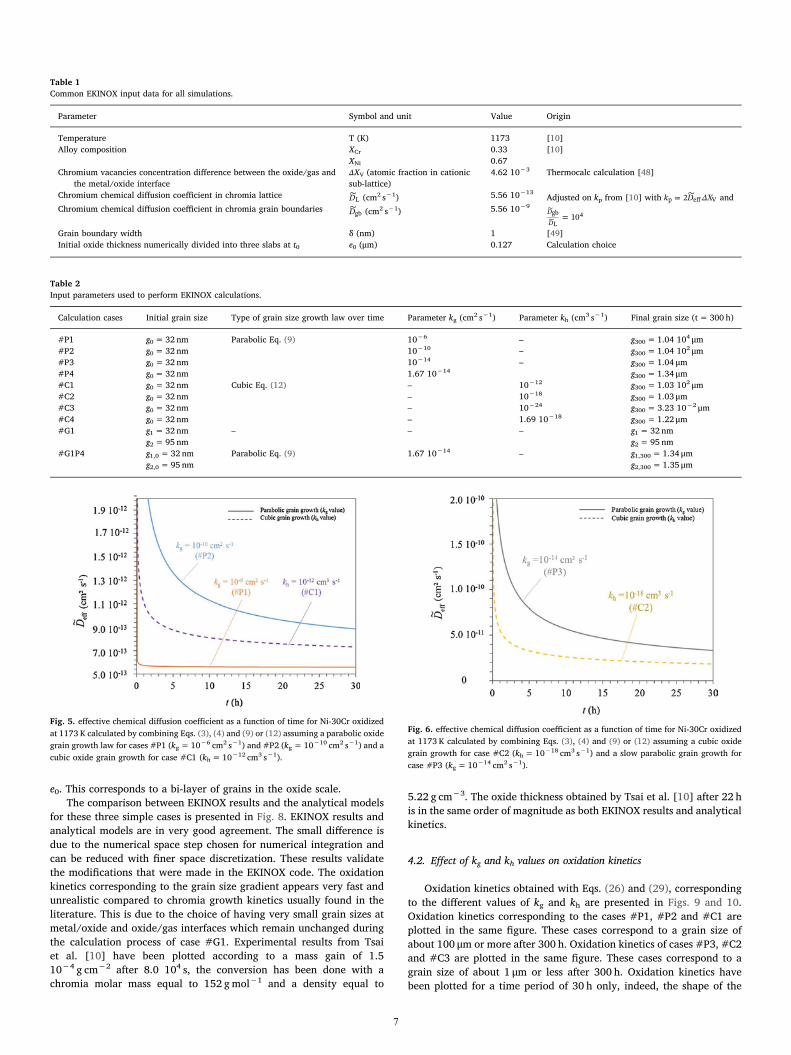
For each case, the effective diffusion coefficient is calculated bycombining Eqs. (3), (4) and (9) or (12). The effective diffusion coeffi-cients for each case are plotted in Figs. 5–7. When the grain growth isfast, both the proportion of short-circuit diffusion and the effectivediffusion coefficient decrease rapidly. As a result, the faster the oxidegrain growth the larger slowing effect on the oxidation kinetics.
4. EKINOX results
This section focuses on the results of EKINOX calculations. The firstpart deals with the validation of the numerical calculations. Oxidationkinetics obtained with EKINOX are compared with the analytical oxi-dation kinetics represented by Eq. (26), (29) and (34). The second partpresents the comparison of several EKINOX kinetics obtained for dif-ferent types of grain size evolution: case #P4 corresponds to a parabolicgrain growth, case #G1 corresponds to a grain size gradient, and case#G1P4 corresponds to a combination of a parabolic grain growth and agrain size gradient. Finally, a parametric study is carried out regardingthe influence of kg and kh parameters on the oxidation kinetics of dif-ferent cases: #P1, #P2, #P3 and #C1, #C2, #C3.
4.1. Comparison between EKINOX and analytical models
The initial grain size chosen for the comparison of these differentcases is g0= 32 nm. The growth grain constants kg and kh are chosen toreproduce the order of magnitude of the average oxide/gas grain sizeobserved experimentally by Tsai et al. [10] after 165 h, which is∼1 μm. kg and kh values are respectively 1.67 10−14 cm2 s−1 for case#P4 and 1.69 10−18 cm3 s−1 for case #C4. For the case assuming agrain size gradient within the oxide scale #G1, the chosen grain sizesare g1= 32 nm at the metal/oxide interface and g2= 95 nm at theoxide/gas interface.
These grain sizes were calculated to have a ratio of three between g1and g2, and so that the sum of g1 and g2 equals the initial oxide thickness
Fig. 4. Schematic representation of oxide/metal system in EKINOX model.
6
e0. This corresponds to a bi-layer of grains in the oxide scale.The comparison between EKINOX results and the analytical models
for these three simple cases is presented in Fig. 8. EKINOX results andanalytical models are in very good agreement. The small difference isdue to the numerical space step chosen for numerical integration andcan be reduced with finer space discretization. These results validatethe modifications that were made in the EKINOX code. The oxidationkinetics corresponding to the grain size gradient appears very fast andunrealistic compared to chromia growth kinetics usually found in theliterature. This is due to the choice of having very small grain sizes atmetal/oxide and oxide/gas interfaces which remain unchanged duringthe calculation process of case #G1. Experimental results from Tsaiet al. [10] have been plotted according to a mass gain of 1.510−4 g cm−2 after 8.0 104 s, the conversion has been done with achromia molar mass equal to 152 gmol−1 and a density equal to
5.22 g cm−3. The oxide thickness obtained by Tsai et al. [10] after 22 his in the same order of magnitude as both EKINOX results and analyticalkinetics.
4.2. Effect of kg and kh values on oxidation kinetics
Oxidation kinetics obtained with Eqs. (26) and (29), correspondingto the different values of kg and kh are presented in Figs. 9 and 10.Oxidation kinetics corresponding to the cases #P1, #P2 and #C1 areplotted in the same figure. These cases correspond to a grain size ofabout 100 μm or more after 300 h. Oxidation kinetics of cases #P3, #C2and #C3 are plotted in the same figure. These cases correspond to agrain size of about 1 μm or less after 300 h. Oxidation kinetics havebeen plotted for a time period of 30 h only, indeed, the shape of the
Table 1Common EKINOX input data for all simulations.
Parameter Symbol and unit Value Origin
Temperature T (K) 1173 [10]Alloy composition XCr 0.33 [10]
XNi 0.67Chromium vacancies concentration difference between the oxide/gas and
the metal/oxide interfaceΔXV (atomic fraction in cationicsub-lattice)
4.62 10−3 Thermocalc calculation [48]
Chromium chemical diffusion coefficient in chromia lattice ∼DL (cm2 s−1) 5.56 10−13Adjusted on kp from [10] with = ∼k D ΔX2p eff V and
=∼
∼ 10D
Dgb
L4
Chromium chemical diffusion coefficient in chromia grain boundaries ∼Dgb (cm2 s−1) 5.56 10−9
Grain boundary width δ (nm) 1 [49]Initial oxide thickness numerically divided into three slabs at t0 e0 (μm) 0.127 Calculation choice
Table 2Input parameters used to perform EKINOX calculations.
Calculation cases Initial grain size Type of grain size growth law over time Parameter kg (cm2 s−1) Parameter kh (cm3 s−1) Final grain size (t= 300 h)
#P1 g0= 32 nm Parabolic Eq. (9) 10−6 – g300= 1.04 104 μm#P2 g0= 32 nm 10−10 – g300= 1.04 102 μm#P3 g0= 32 nm 10−14 – g300= 1.04 μm#P4 g0= 32 nm 1.67 10−14 g300= 1.34 μm#C1 g0= 32 nm Cubic Eq. (12) – 10−12 g300= 1.03 102 μm#C2 g0= 32 nm – 10−18 g300= 1.03 μm#C3 g0= 32 nm – 10−24 g300= 3.23 10−2 μm#C4 g0= 32 nm – 1.69 10−18 g300= 1.22 μm#G1 g1= 32 nm – – – g1= 32 nm
g2= 95 nm g2= 95 nm#G1P4 g1,0= 32 nm Parabolic Eq. (9) 1.67 10−14 – g1,300= 1.34 μm
g2,0= 95 nm g2,300= 1.35 μm
Fig. 5. effective chemical diffusion coefficient as a function of time for Ni-30Cr oxidizedat 1173 K calculated by combining Eqs. (3), (4) and (9) or (12) assuming a parabolic oxidegrain growth law for cases #P1 (kg= 10−6 cm2 s−1) and #P2 (kg= 10−10 cm2 s−1) and acubic oxide grain growth for case #C1 (kh= 10−12 cm3 s−1).
Fig. 6. effective chemical diffusion coefficient as a function of time for Ni-30Cr oxidizedat 1173 K calculated by combining Eqs. (3), (4) and (9) or (12) assuming a cubic oxidegrain growth for case #C2 (kh= 10−18 cm3 s−1) and a slow parabolic grain growth forcase #P3 (kg= 10−14 cm2 s−1).
7

curves are more visible over short periods of time.The higher the value of kg or kh, the slower the oxidation kinetics.
This tendency was expected. It seems interesting however to notice thatthe general shape of the oxidation curves evolves with the chosen valueof kg or kh. For cases #P3 and #C3, which have the lowest values of kgand kh respectively, oxidation kinetics move away from a parabolic lawand appears to be more of a sub-parabolic pattern as shown in Fig. 10.For the highest values of kg and kh: 10−6 cm2 s−1 and 10−12 cm3 s−1
respectively, oxidation kinetics look like a parabolic law as shown inFig. 9. For the intermediate values of kg and kh: 10−10 cm2 s−1 and10−18 cm3 s−1 respectively, oxidation kinetics seem to display inter-mediate shapes as shown in Figs. 9 and 10 respectively.
4.3. Study of the combined effect of grain size gradient within the oxidescale and parabolic grain growth
In this part the three following cases were treated: (1) a parabolicgrain growth law for case #P4 according to Eq. (9) withkg= 1.67 10−14 cm2 s−1, (2) a grain size gradient for case #G1 withg1= 32 nm and g2= 95 nm; and (3) a combination of parabolic grainsize growth and grain size gradient for case #G1P4. These differentoxidation kinetics are presented in Fig. 11. They are plotted over shortoxidation time periods of up to 20 h: this time window corresponds tothe interest zone for the simulation parameters chosen.
During the very early stages of oxidation (up to 2 h), the oxidethickness corresponding to a parabolic growth law for case #P4 ishigher than the oxide thickness corresponding to the grain size gradientfor case #G1. After two hours, this tendency is reversed and the oxidethickness corresponding to the grain size gradient for case #G1 be-comes higher than the oxide thickness corresponding to the parabolicgrain size growth for case #P4. This result shows that the two oxidationkinetics do not follow the same law. According to Eq. (26), the oxida-tion kinetics corresponding to a parabolic grain size growth is sub-parabolic, whereas according to Eq. (34), the oxidation kinetics corre-sponding to a grain size gradient remains purely parabolic.
Concerning case #G1P4, with the combination of parabolic grainsize growth and grain size gradient, the oxide thickness is alwayssmaller than that of the two other cases. This result was expected sincein this case, the grain size cumulates both growth effects: in time and inspace. The proportion of short-circuit diffusion is thus the lowest of thethree cases. A similar conclusion can be made for a cubic grain growthlaw instead of a parabolic grain growth law.
Results from this section can be summarized as follows:
Fig. 7. effective chemical diffusion coefficient as a function of time for Ni-30Cr oxidizedat 1173 K calculated by combining Eqs. (3), (4) and (12) assuming a slow cubic graingrowth law for case #C3 (kh=10−24 cm3 s−1).
Fig. 8. chromia growth kinetics on Ni-30Cr at 1173 K calculated with EKINOX andanalytical models with g0= 32 nm, and kp,L= 1.18 10−14 cm2 s−1 for different hy-potheses: a parabolic grain size growth for case #P4 according to Eq. (9) withkg= 1.67 10−14 cm2 s−1, a cubic grain growth law for case #C4 according to Eq. (12)with kh= 1.69 10−18 cm3 s−1, and a grain size gradient for case #G1 with g1= 32 nmand g2= 95 nm. An experimental data [10] is also displayed.
Fig. 9. oxidation kinetics of Ni-30Cr oxidized at 1173 K calculated with Eqs. (26) or (29)assuming a parabolic oxide grain growth law for cases #P1 (kg= 10−6 cm2 s−1) and #P2(kg= 10−10 cm2 s−1) and cubic oxide grain growth for case #C1 (kh= 10−12 cm3 s−1).
Fig. 10. oxidation kinetics of Ni-30Cr oxidized at 1173 K, calculated with Eqs. (26) and(29) assuming a parabolic grain growth for case #P3 (kg= 10−14 cm2 s−1) and a cubicgrain growth for cases #C2 (kh= 10−18 cm3 s−1) and #C3 (kh= 10−24 cm3 s−1).
8

- A parametric study with analytical calculations showed that kg andkh parameters, which characterize the grain growth rate, can have amajor influence on the shape of oxidation kinetic curves whenconsidering the grain boundaries as a fast diffusion path.
- EKINOX calculations taking into account the combined effect ofgrain growth and grain size gradient across the oxide scale for case#G1P4, show that the resulting oxidation kinetics are closer to theoxidation kinetics corresponding to the grain size gradient only forcase #P4 for short times, and closer to the oxidation kinetics cor-responding to grain growth only for case #G1 for longer times.
Considering these points, it is interesting to discuss post-treatmentmethods of oxidation kinetics curves as well as derived extrapolationsover a longer time range.
5. Discussion
The aim of this discussion is to compare two different methods ofinterpretation and extrapolation of experimental oxidation kinetics: the“log-log” method and the “parabolic law” method. To do so, the resultsof the previous calculations are used as if they were experimental data.
5.1. Estimation of the parabolic rate constant values (kp) from calculatedkinetic curves
In this paragraph, oxidation kinetics simulated with EKINOX pre-sented in the previous section are post-treated according to the “para-bolic law” method with the local kp calculation method [43]. Thismethod is presented in Section 2.6.1. The oxidation kinetics consideredfor the calculation of local kp values for cases #P4, #G1 and #G1P4 areplotted in Fig. 11. Corresponding local values of kp are plotted over timein Fig. 12.
The local kp value corresponding to case #G1 with grain size gra-dient across the oxide scale but without grain growth is constant. Thisresult could have been predicted as the corresponding kinetics follows apure parabolic law as determined in Eq. (34). The local kp value cor-responding to the combination of a parabolic grain growth and a grainsize gradient for case #G1P4, is close to the local kp curve corre-sponding to a parabolic grain growth # P4. These two local kp curvescorresponding to cases with a grain size evolution over time: cases #P4and #G1P4, decrease rapidly of about one order of magnitude duringthe first hour of oxidation. It shows that for short time experiments thegrain growth can strongly affect the value of the parabolic rate constantdetermined by a classical fit on the whole kinetic curve. The fact that
the value of kp changes over time could explain the discrepancy of kpvalues found in the literature for different oxidation times as presentedin Fig. 1.
5.2. Treatment of oxidation kinetics obtained with EKINOX simulations,using several values for kg and kh
5.2.1. Log-log methodThe usual way of using the “log-log” method is to perform a linear
fit in a log–log plot on the whole kinetic curve. The “log-log” method isexplained more extensively on Section 2.6.2. This method over-estimates the weight of short times on the global interpretation becauseof the logarithm function. For long term extrapolation, a more accuratedescription of oxidation kinetics can be obtained by admitting the ex-istence of a transitory regime for short times. Thus, linear fits are per-formed on the final portions of the plots, which better describe thestationary regime. In this part, the extrapolation using the “log-log”method is compared to the extrapolation using the “parabolic law”method that also uses the final part of the oxidation kinetic curve. For afair comparison, this is carried out on the same time interval.
Examples of calculated oxidation kinetics are post-treated with the“log-log” method in Fig. 13 for the parabolic grain growth cases: #P1,#P2, and #P3. Linear fits are performed on a time range from 25 to30 h. According to the “log-log” method, the parameters m and klogfrom Eqs. (24) and (25) can be obtained. These values for the differentoxidation kinetics corresponding to the different values of kg and kh aregathered in Table 3.
The parameter m reflects the shape of the oxidation kinetics as itcorresponds to the value of the time exponent parameter according toEq. (24). For the fastest grain growth conditions: #P1 withkg= 10−6 cm2 s−1 and #C1 with kh= 10−12 cm3 s−1, the m parameterequals 1.4 and 1.7 respectively, that means that the shape of the oxi-dation kinetics can be bounded between a linear dependence with timeand a square root dependence with time. The global oxidation kineticscould thus be interpreted as an over-parabolic law. For the intermediaterate of grain growth with kg= 10−10 cm2 s−1 and the case withkh= 10−18 cm3 s−1 corresponding to cases # P2 and #C2 respectively,the m value equals 2.15, and 2.8 respectively, that means that the shapeof the oxidation kinetics can be bounded between a square root de-pendence with time and a cubic root dependence with time. The oxi-dation kinetic law can be interpreted as parabolic (if m parameter isclose to 2) or as an intermediate law between parabolic and cubic. Forthe slowest grain growth rate: case #P3 with kg= 10−14 cm2 s−1, the mparameter equals 3.8, that means that the shape of the oxidation
Fig. 11. chromia growth kinetics of Ni-30Cr at 1173 K calculated with the EKINOX modelcorresponding to different hypotheses: a parabolic grain size growth for case #P4(kg= 1.67 10−14 cm2 s−1), a grain size gradient for case #G1 with g1= 32 nm andg2= 95 nm, and a combination of the parabolic grain size growth and grain size gradientfor case #G1P4.
Fig. 12. local kp from chromia growth kinetics of Ni-30Cr at 1173 K, calculated with theEKINOX model corresponding to a parabolic grain growth for case #P4(kg= 1.67 10−14 cm2 s−1), a grain size gradient for case #G1 with g1= 32 nm andg2= 95 nm, and a parabolic grain size growth combined with a grain size gradient forcase #G1P4.
9

kinetics can be bounded between a cubic root dependence with timeand a fourth root dependence with time. In this case, the oxidationkinetics is close to a quadratic law as the m parameter is close to 4.Finally for the slowest cubic growth rate: case #C3 withkh= 10−24 cm3 s−1, the m parameter equals 3.0, the oxidation kineticlaw can be interpreted as cubic, the shape of the oxidation kinetics canbe approximated by a cubic root dependence with time. This last par-ticular case matches Rhines' observations [23,24] with a cubic graingrowth law associated with a cubic oxidation kinetics. The grain size isthus proportional to the oxide thickness.
By using the “log-log” method, oxidation kinetics could be plottedwith an over-parabolic, cubic or quadratic law despite the fact thatgrowth mechanisms remain identical (only kinetic constants change).
These results can be explained by means of the analytical oxidationmodels presented in part II of this work: Eq. (26) for a parabolic oxidegrain growth and Eq. (29) for a cubic oxide grain growth. The oxidationkinetic law given by Eq. (26) is composed of three terms. One termproportional to time, one term proportional to the square root of time,and one constant term. Depending on the values of the parameters ofthe law, one term of the kinetic law can become predominant comparedto the others for a given time range, and the global oxidation kineticsfollows the tendency given by the predominant term. If the pre-dominant term is the one proportional to time, the global oxidation
kinetics has a parabolic pattern, for example #P1 withkg= 10−6 cm2 s−1. If the predominant term is the one proportional tothe square root of time, the global oxidation kinetics has a quadraticpattern, for example #P3 with kg= 10−14 cm2 s−1. Transition values ofkg and kh from one type of law to the other can be determined for agiven duration of the experiment. This calculation is described inAppendix B.
Some oxide thickness extrapolations from 30 h oxidation kineticscan be calculated according to kinetic laws using Eq. (24) with the datagathered in Table 3. The corresponding extrapolated oxide thickness for1 year and 10 years of oxidation are gathered in Table 3. For compar-ison, real thicknesses from analytical laws (26) and (29) are also re-ported. Relative errors in the extrapolation range from 0.1% to 217%.The gap between extrapolated and analytical values increases withlonger extrapolation times and with the values of kg and kh. Indeed, therelative error is the highest for cases #P1 and #C1, which correspondrespectively to the highest values of kg and kh.
5.2.2. Complete parabolic law methodAnother post-treatment method applied to kinetic curves has been
carried out by using Eq. (22), which corresponds to the completeparabolic law. This law has been adjusted to fit the curves on the sametime interval as determined previously (for the “log-log” method): from25 to 30 h. kp,(25h), values obtained following these adjustments arelisted in Table 3.
kp,(25h) values given in Table 3 and obtained in the 25–30 h timeperiod are higher for cases with the lowest values of kg and kh. As grainsize increases continuously over time, the local kp value decreases overtime, and for a long enough time, the second part of Eqs. (26) and (29)become negligible compared to the first part of the relations. The kp,statvalue is expected to reach kp,L= 8.10−15 cm2 s−1 for an infinite time. Asimilar observation can be made on the values of the effective diffusioncoefficient plotted in Figs. 5–7, which decrease over time with the graingrowth. The effective diffusion coefficients are obviously expected toreach the lattice diffusion coefficient for an infinite time. In the casesstudied here, the time needed to reach this stationary regime dependson grain growth kinetics, and is thus linked to the values of kg and kh. Ifthe grain growth is fast, the effective diffusion coefficient quicklyreaches its stationary value. In contrast, if the grain growth is slow, theeffective diffusion coefficient reaches its stationary value after a longtime.
The kp,(25h) values obtained by parabolic fit gathered in Table 3 forcases #P1, #P2 and #C1 are of the same order of magnitude askp,L= 8.10−15 cm2 s−1. It can thus be assumed that, in these cases, thestationary regime is reached after 25 h. For cases #P3, #C2 and #C3however, the local kp value is different from the kp,L value, ranging fromone to three orders of magnitude. This is due to the fact that the sta-tionary regime has not been reached after 25 h. The kp values obtained
Fig. 13. oxidation kinetics of Ni-30Cr at 1173 K, calculated with Eq. (26), plotted on alog–log scale (e-e0 (cm), t(s)) assuming a parabolic growth law according to Eq. (9), andfor kg values of 10−14 cm2 s−1, 10−10 cm2 s−1 and 10−6 cm2 s−1. Linear fits are done forthe time interval going from 25 to 30 h. Solid lines correspond to calculated kinetics,dotted lines to linear fits.
Table 3Analytical oxide thickness calculated with Eqs. (26) and (29) respectively for parabolic grain growth #P1, #P2, #P3 and cubic grain growth #C1, #C2, #C3. m, klog, and kp,(25h)parameters are obtained from extrapolations of analytical oxidation kinetics of Ni-30Cr on 30 h at 1173 K according to “log-log” and “parabolic law” methods. Extrapolated oxidethicknesses corresponding to “log-log” and “parabolic law” extrapolation methods according to Eqs. (24) and (22) and calculated with parameters m, klog and kg,(25h) are given for 1 yearand 10 years. Finally, relative errors on oxide thickness between analytical and extrapolated values are given.
log–log method Parabolic law method
Calculation case Oxide grain growthparameter
Analytical oxidethickness (μm)
m klog elog-log (μm) Relative error onoxide thickness (%)
kp,(25h) = 1/C(cm2 s−1)
eparablaw (μm) Relative error onoxide thickness (%)
1 year 10 years 1 year 10 years 1 year 10 years 1 year 10 years 1 year 10 years
#P1 kg(cm2 s−1)
10−6 5.0 15.9 1.4 2.10−12 10.2 50.4 104 217 8.10−15 4.9 15.8 2 0.6#P2 10−10 5.2 16.1 2.15 4.10−15 4.8 14.3 8 11 8.10−15 5.1 16.0 2 0.6#P3 10−14 14.2 28.4 3.8 4.10−19 13.8 25.2 3 11 8.10−14 18.0 51.7 27 82#C1 kh
(cm3 s−1)10−12 5.2 16.2 1.7 2.10−13 7.6 29.6 46 83 9.10−15 5.3 16.5 2 2
#C2 10−18 14.4 33.1 2.8 4.10−16 14.8 33.7 3 2 9.10−14 18.2 54.6 21 67#C3 10−24 135.1 291.3 3.0 9.10−14 135.0 292.2 0.1 0.3 8.10−12 177.4 529.6 31 82
10

by parabolic fit for these three cases thus do not correspond to thestationary kp value. Consequently the parabolic extrapolation is notcorrect and should not be employed in these cases. The evolution oflocal kp values of cases #P1 and #C3 are plotted in Fig. 14. In case #P1,local kp is stationary throughout the entire time range chosen, whereasin case #C3, the value of kp decreases dramatically at early oxidationtimes and is still decreasing at the end of the experiment. This illustratesthat the stationary value of kp has not been reached at the end of theoxidation time chosen here.
The oxide thickness can be extrapolated using complete paraboliclaws with Eq. (22) and parameters given in Table 3. This same tabledisplays the values of these extrapolated oxide thicknesses for 1 yearand 10 years, and the corresponding analytical values calculated withEqs. (26) and (29). The relative errors between extrapolated and ana-lytical values range from 0.6% and 82%. Contrary to the extrapolationsobtained with the “log-log” method, discrepancies increase as values ofkg or kh decrease. Indeed, the most important relative errors are foundfor cases #P3, #C2 and #C3, those with the slowest grain growth rate,and therefore having the longest transient stage of oxidation. For theslowest grain growth rates, the oxidation kinetics is far from the para-bolic regime, even over a long time range. As shown in Fig. 14 with case#C3, local kp had still not reached its stationary value after 25 h.
To conclude this part, the best way to fit the experimental data is touse the local kp method first, in order to determine if the parabolicstationary regime is reached. If so, the best extrapolation is given by thecomplete parabolic law using the value of kp obtained for the stationaryregime, i.e. kp,stat. This method is more accurate than the one that uses apower law, even if this latter has been obtained by a fit over longeroxidation times. If no parabolic stationary regime can be determined forthe local kp curve, as is the case for very slow grain growth rates, it canbe then more appropriate to use the “log-log” method for extrapolation.
However, when possible, the best method is to perform a longer ex-periment until the stationary regime is reached, and to extrapolate withthe “parabolic law” method using the stationary kp and the completelaw. The alternative method consists in using an analytical or numericalmodel that includes grain growth kinetics, if the evolution of local kp isassumed to be due to the oxide grain size evolution.
6. Conclusion
The conclusions that can be drawn from this work are the following:
1) Grain boundary diffusion and oxide scale microstructure evolutionover time should be considered to interpret oxidation kinetics whichare not purely parabolic.
2) Analytical models are presented considering a cubic grain growthlaw and a grain size gradient across the oxide scale. A numericalresolution, using for example the EKINOX model, can be used tosimulate more complex cases of combination of grain size growthand grain size gradient but also other grain size growth laws.
3) Calculation results show that even when using the same oxidegrowth mechanism, i.e. control by faster diffusion in the oxide dueto grain boundaries diffusion, the evolution rate of diffusion short-circuit proportion over time modifies the oxide growth kinetics, andeven their global shapes.
4) Depending on grain growth kinetics, the experimental oxidationkinetics that derive from a mixed diffusion phenomenon in bulk andin grain boundaries can be globally interpreted with various lawsfrom over-parabolic to parabolic, sub-parabolic, cubic and evenquadratic.
5) Extrapolation of oxidation kinetics can be strongly affected by thechoice of the method, and also by the duration of the oxidationexperiment. The use of the “local kp” helps identifying if the para-bolic stationary regime is reached and thus helps performing accu-rate extrapolations of oxidation kinetics. If the stationary regime isnot reached during the oxidation time of the experiment, no extra-polation should be done. If longer experiment cannot be performed,extrapolation using the “log-log” method might be a better choice.However, experimenters have to keep in mind that this extrapola-tion is not based on clearly identified rate controlling phenomenaand then should be used with caution.
This study focuses on the growth of chromia, however, similarconclusions can be drawn on the growth of other oxides.
Acknowledgments
S. Gossé, C. Gueneau, P. Zeller and A. Chartier (CEA), forThermocalc calculations and constructive discussions are gratefullyacknowledged.
Appendix A. Symbols used
A, B, C: coefficients used for the “complete parabolic law fit” (respectively in s, s cm−1, s cm−2)XA
n: atomic site fraction of A in the slab n in the EKINOX modelXA: atomic site fraction of A (A=Cr or Ni) in alloyCX
n: site fraction for specie X calculated on EKINOX model in slab n (dimensionless)∼Deff : effective chemical diffusion coefficient (cm2 s−1)∼Dgb: grain boundary chemical diffusion coefficient (cm2 s−1)∼DL: chemical diffusion coefficient in oxide lattice (cm2 s−1)JX
n: flux of specie X calculated on EKINOX model in slab n (site m−2 s−1)e: oxide scale thickness, e0 corresponds to oxide thickness at initial time t0 (cm)f: atomic site fraction on short-circuits path per unit area (dimensionless)g: grain size, g0 grain size at initial time t0, g1 corresponds to oxide grain size at metal/oxide interface, g2 corresponds to oxide grain size at oxide/
gas interface (cm)
Fig. 14. local kp value corresponding to the oxidation kinetics of Ni-30Cr at 1173 K,calculated with Eqs. (26) and (29), corresponding respectively to kg= 10−6 cm2 s−1 forcase #P1 (scale on the left) and kh= 10−24 cm3 s−1 for case #C3 (scale on the right).
11

kg: parabolic coefficient for the grain growth law (cm2 s−1)kh: cubic coefficient for the grain growth law (cm3 s−1)kl: linear constant of the oxide scale growth (cm s−1) or (g cm−2 s−1)klog: kinetic parameter used for the power law kinetics of oxide scale growth (“log-log” method) (units depend on exponent of the power law: m)kp: parabolic constant of the oxide scale growth, kp,eff corresponds to effective parabolic constant in case of diffusion through lattice and grain
boundaries, kp,I corresponds to instantaneous parabolic constant of the oxide scale growth, kp,L corresponds to parabolic constant of the oxide scalegrowth in case of diffusion through lattice only, kp,stat corresponds to local parabolic constant corresponding to the stationary regime of the oxidescale growth (cm2 s−1) or (g2 cm−4 s−1)
m: exponent used for the power law kinetics of oxide scale growth (“log-log” method) (dimensionless)t: time, t0 corresponds to initial time (s) or (h)x: position in the oxide scale (cm)δ: short-circuit thickness, or grain boundary thickness (cm)ΔC: difference in defect concentration between the oxide/gas interface and the metal/oxide interface (atom cm−3)Δm: mass gain per unit area, Δmi corresponds to initial mass gain per unit area (g cm−2)ΔXV: difference between vacancy site fraction at oxide/gas and metal/oxide interfaces (dimensionless)Δy: difference of relative position in oxide scale (dimensionless)Ω: volume of oxide per oxide site (cm3 atom−1)
Appendix B. Calculation of transition kg and kh values
With an oxidation time of 30 h, a transition kg value, so called kgtr can be determined for transition between predominance of the square root part
of time. Right side of Eq. (26) and predominance of the linear part of time i.e. left side of Eq. (26).
+ = −∼
∼k t e t( 1)δk
k
D
Dp,L 02 4 p,L
gtr
gb
L(39)
leading to:
=⎛
⎝
⎜⎜ +
−⎞
⎠
⎟⎟
∼
∼kδk
k t
DD
4( 1)
et
gtr p,L
p,L
gb
L
2
02
(40)
Following the same approach, the transition value of the cubic growth rate of grain size khtr leading to different regimes of oxidation kinetics can
be determined:
=⎛
⎝
⎜⎜ +
−⎞
⎠
⎟⎟
∼
∼kδk
k t
DD
3( 1)
e
t
tr p,L
p,L1/3
gb
L
3
h02
2/3 (41)
By using the parameters chosen in this study for case #P2, with kg= 10−10 cm2 s−1, global oxidation kinetics have a mixed parabolic andquadratic tendency. For parameters corresponding to case #C2, with kh= 10−18 cm3 s−1, oxidation kinetics have a mixed parabolic and cubictendency.
In order to have the time proportionate term predominant in Eq. (26), the value of kg value must respect the condition: kg > > kgtr, this
corresponds to case #P1, with kg= 10−6 cm2 s−1. By using a similar approach for a cubic oxide grain growth law, the condition kh > > khtr
corresponds to case #C1, with kh= 10−12 cm3 s−1. These cases lead to oxidation kinetics following a parabolic law.In order to have the term proportional to the square root of time predominant in Eq. (26), the value of kg must respect the condition: kg < < kg
tr,this corresponds to case #P3, with kg= 10−14 cm2 s−1. By using a similar approach for a cubic oxide grain growth law, the condition kh > > kh
tr
corresponds to case #C3, with kh= 10−24 cm3 s−1. These cases lead to oxidation kinetics following a quadratic and a cubic law respectively.
Data availability
The processed data (output of EKINOX code) required to reproduce these findings, which are oxide thicknesses over time, and effective diffusioncoefficient, are already shared in graphs in Figs. 8 and 11.
References
[1] A. Atkinson, R.I. Taylor, G. Simkovich, V.S. Stubican (Eds.), Transport inNonstoichiometric Compounds, vol. 129, 1985, pp. 285–295.
[2] K.P. Lillerud, P. Kofstad, J. Electrochem. Soc. 127 (1980) 2410–2419.[3] D.J. Young, M. Cohen, J. Electrochem. Soc. 124 (1977) 769–774.[4] L. Cadiou, J. Paidassi, Mem. Scient. De La Revue De Metall. 66 (3) (1969) 217–225.[5] D. Caplan, G.I. Sproule, Oxid. Met. 9 (5) (1975) 459–472.[6] C.A. Phalnikar, E.B. Evans, W.M. Baldwin, J. Electrochem. Soc. 103 (1956)
429–438.[7] E.A. Gulbransen, K.F. Andrew, J. Electrochem. Soc. 99 (10) (1952) 402–406.[8] K. Taneichi, T. Narushima, Y. Iguchi, C. Ouchi, Materi. Trans. 47 (10) (2006)
2540–2546.[9] A.C.S. Sabioni, J.N.V. Souza, V. Ji, F. Jomard, V.B. Trindade, J.F. Carneiro, Solid
State Ionics 276 (2015) 1–8.
[10] S.C. Tsai, A.M. Huntz, C. Dolin, Mater. Sci. Eng. A 212 (1996) 6–13.[11] A.M. Huntz, A. Reckmann, C. Haut, C. Sévérac, M. Herbst, F.C.T. Resende,
A.C.S. Sabioni, Mater. Sci. Eng. A 447 (1–2) (2007) 266–276.[12] M. Kemdehoundja, J.F. Dinhut, J.L. Grosseau-Poussard, M. Jeannin, Mater. Sci.
Eng. A435 (2006) 666–671.[13] E. Schmucker, C. Petitjean, L. Martinelli, P.J. Panteix, S. Ben Lagha, M. Vilasi,
Corros. Sci. 111 (2016) 474–485.[14] W.C. Hagel, A.U. Seybolt, J. Electrochem. Soc. 108 (12) (1961) 1146–1152.[15] G.M. Ecer, G.M. Meier, Oxid. Met. 13 (2) (1979) 119–158.[16] L. Latu-Romain, Y. Parsa, S. Mathieu, M. Vilasi, A. Galerie, Y. Wouters, Corros. Sci.
126 (2017) 238–246.[17] R.E. Lobnig, H.P. Schmidt, K. Hennesen, H.J. Grabke, Oxid. Met. 37 (1/2) (1992)
81–93.[18] J.M. Perrow, W.W. Smeltzer, J.D. Embury, Acta Metall. 16 (1968) 1209–1218.[19] E. Essuman, G.H. Meier, J. Zurek, M. Hansel, T. Norby, L. Singheiser,
W.Q. Quadakkers, Corros. Sci. 50 (2008) 1753–1760.
12
[20] K. Przybylski, G.J. Yurek, J. Electrochem. Soc. 135 (2) (1988) 517–523.[21] E.W. Hart, Acta Metall. 5 (1957) 595.[22] R.J. Hussey, G.I. Sproule, D. Caplan, M.J. Graham, Oxid. Met. 11 (2) (1977) 65–79.[23] F.N. Rhines, R.G. Connell Jr., J. Electrochem. Soc. 124 (1977) 93–105.[24] F.N. Rhines, R.G. Connell Jr., M.S. Choi, J. Electrochem. Soc. 126 (6) (1979)
1061–1066.[25] D.E. Davies, U.R. Evans, J.N. Agar, Proc. Roy. Soc. A225 (1954) 443–462.[26] W.W. Smeltzer, R.R. Haering, J.S. Kirkaldy, Acta Metall. 9 (1961) 880–885.[27] S. Hallström, M. Halvarsson, L. Höglund, T. Jonsson, J. Agren, Solid State Ionics 240
(2013) 41–50.[28] P. Kofstad, K.P. Lillerud, J. Electrochem. Soc. 127 (11) (1980) 2410–2419.[29] M.W. Barsoum, J. Electrochem. Soc. 148 (2001) C544–C550.[30] J.L. Smialek, Corros. Sci. 91 (2015) 281–286.[31] R. Peraldi, D. Monceau, B. Pieraggi, Oxid. Met. 58 (2002) 249–273.[32] D. Naumenko, B. Gleeson, E. Wessel, L. Singheiser, W.J. Quadakkers, Metall. Mater.
Trans. A 38A (2007) 2974–2983.[33] H. Larsson, T. Jonsson, R. Naraghi, Y. Gong, R.C. Reed, J. Agren, Mater. Corros. 68
(2) (2017) 133–142.[34] T.J. Nijdam, W.G. Sloof, Acta Mater. 55 (2007) 5980–5987.[35] T.J. Nijdam, L.P.H. Jeurgens, W.G. Sloof, Acta Mater. 51 (2007) 5295–5307.[36] C. Desgranges, N. Bertrand, K. Abbas, D. Monceau, D. Poquillon, et al., P. Steinmetz
(Ed.), High Temperature Corrosion and Protection of Materials 6, Prt 1 and 2,Proceedings, Trans Tech Publications Ltd, 2004, pp. 481–488 461–464.
[37] N. Bertrand, C. Desgranges, M. Nastar, G. Girardin, D. Poquillon, D. Monceau,
P. Steinmetz, I.G. Wright, A. Galerie, D. Monceau, S. Mathieu (Eds.), HighTemperature Corrosion and Protection of Materials 7, Pts 1 and 2, Trans TechPublications Ltd, 2008, pp. 463–472 595–598.
[38] C. Desgranges, F. Lequien, E. Aublant, M. Nastar, D. Monceau, Oxid. Met. 79 (2013)93–105.
[39] Y. Adda, J. Philibert, La Diffusion dans les solides Bibliothèque Des Sciences EtTechniques Nucléaires, Institut National Des Sciences Et Techniques Nucléaires &Presses Universitaires De France, Paris, 1966.
[40] C. Wagner, Zeitshrift für Physik B21 (25) (1933).[41] I. Kaur, Y. Mishin, W. Gust, Fundamentals of Grain and Interphase Boundary
Diffusion, John Wiley, 1995.[42] L.G. Harrison, Trans. Faraday Soc. 57 (1961) 1191–1199.[43] D. Monceau, B. Pieraggi, Oxid. Met. 50 (1998) 477–493.[44] B. Pieraggi, Oxid. Met. 27 (1987) 177–185.[45] A. Atkinson, R.I. Taylor, A.E. Hugues, Philos. Mag. A 45 (5) (1982) 823–833.[46] J. Zurek, D.J. Young, E. Essuman, M. Hänsel, H.J. Penkalla, L. Niewolak,
W.J. Quadakkers, Mater. Sci. Eng. A 477 (2008) 259–270.[47] D.J. Young, D. Naumenko, L. Niewolak, E. Wessel, L. Singheiser, W.J. Quadakkers,
Mater. Corros. 61 (10) (2010) 838–844.[48] L. Kjellqvist, M. Selleby, CALPHAD 33 (2009) 393–397.[49] A.C.S. Sabioni, R.P.B. Ramos, V. Ji, F. Jomard, W.A.A. Macedo, P.L. Gastelois,
V.B. Trindade, Oxid. Met. 78 (2012) 211–220.[50] A. Atkinson, Oxid. Met. 28 (5/6) (1987) 353–389.
13