modelling of stormwater overland flow in urban areas
TRANSCRIPT

Modelling of stormwater overland
flow in urban areas
Final, 20 January 2012 T.M. Klok


Modelling of stormwater overland
flow in urban areas
Assessment of WOLK as an overland flow modelling
tool

Modelling of stormwater overland flow in urban areas
5\107
Responsibility
Title Modelling of stormwater overland flow in urban areas
Author(s) T.M. Klok
Project number 0322009
Number of pages 113 (excluding appendices)
Date 20 January 2012
Colophon
Timon Klok Supervisors: University of Twente dr. ir. D.C.M. Augustijn dr. ir. P.C. Roos Tauw bv dr. ir. J. Kluck Tauw bv Water department P.O. Box 20748 1001 NS Amsterdam The Netherlands Telephone +31 20 60 63 22 2 Fax number +31 20 68 48 92 1
intellectual property rights. Copyrights to this document remain with Tauw. The quality and continual improvement of products and
processes have the highest priority at Tauw. We operate under a management system that is certified and/or accredited according to:
- NEN-EN-ISO 9001

6\107
Modelling of stormwater overland flow in urban areas T.M.Klok
7\107
Preface Before you lies my master thesis written as the final stage of the specialization „Water Engineering and Management‟ within the master „Civil Engineering and Management‟ at the University of Twente. During the months in which I‟ve been conducting my research and writing this thesis, I learned a lot and gained valuable experiences about the development of overland flow models. The research is performed in cooperation with Tauw. In the company quite some people have helped me with my research. I‟d like to thank all of them for all their time, advice, support and the data they gave me without hesitation. Some people I‟d like to mention personally: Denie Augustijn and Pieter Roos, my mentors at the University of Twente, I‟d like to thank for their constructive feedback, advice, patience and guidance. I‟d also like to thank them for always making time when needed and helping me through the sometimes difficult steps of writing a thesis. I‟d like to thank Jeroen Kluck from Tauw for all his time, ideas and feedback. You were always supportive of my research and helped me with new insights into the world of urban water management. Finally, I‟d like to thank Merijn and my parents who have always believed in me and supported me in every way needed. Without your support I wouldn‟t be where I am now. Timon Klok Enschede, 2012

Modelling of stormwater overland flow in urban areas T.M.Klok
8\107
Contents
Responsibility and Colophon ....................................................................................................... 5
Preface ........................................................................................................................................ 7
Summary ...................................................................................................................................... 11
1 Introduction ................................................................................................................. 15
1.1 Overland flow models .................................................................................................... 16
1.2 Research motivation ...................................................................................................... 16
1.3 Research questions ....................................................................................................... 17
1.4 Methodology .................................................................................................................. 18
1.5 Report outline ................................................................................................................ 19
2 Urban Stormwater Management ................................................................................ 23
2.1 Urban water cycle .......................................................................................................... 23
2.1.1 Precipitation ............................................................................................................... 24
2.1.2 Infiltration .................................................................................................................... 25
2.1.3 Evaporation ................................................................................................................ 25
2.1.4 Sewer system ............................................................................................................. 25
2.1.5 Overland flow ............................................................................................................. 26
2.2 Urban stormwater models ............................................................................................. 26
2.2.1 Model layout ............................................................................................................... 27
2.2.2 Choice of model ......................................................................................................... 27
2.3 User demands ............................................................................................................... 28
2.3.1 Consequences of floods ............................................................................................. 28
2.4 Conclusions ................................................................................................................... 29
3 WOLK ........................................................................................................................... 33
4 Towards a uniform use of WOLK ............................................................................... 37
4.1 Filtering .......................................................................................................................... 37
4.2 Spatial interpolation ....................................................................................................... 38
4.2.1 Spline ......................................................................................................................... 38
4.2.2 Natural Neighbor ........................................................................................................ 39
4.2.3 Inverse Distance Weighting ....................................................................................... 40
4.2.4 Kriging ........................................................................................................................ 41
4.2.5 Overview of results from different interpolation methods in ArcGIS. .......................... 42
Modelling of stormwater overland flow in urban areas T.M.Klok
9\107
4.3 Raster cell size .............................................................................................................. 43
4.4 Conclusions ................................................................................................................... 44
5 Assessment of WOLK ................................................................................................. 47
5.1 Case description ............................................................................................................ 47
5.2 Comparison of WOLK „09 and „11 ................................................................................. 48
5.3 SWOT analysis .............................................................................................................. 53
5.4 Conclusion ..................................................................................................................... 54
6 New model ................................................................................................................... 57
6.1 Computation methodology of new model ...................................................................... 59
6.1.1 Intuitive distribution model .......................................................................................... 59
6.1.2 Manning-based model ................................................................................................ 60
6.2 Numerical scheme ......................................................................................................... 61
6.3 Testing ........................................................................................................................... 64
6.3.1 Results ....................................................................................................................... 65
6.4 Conclusions ................................................................................................................... 66
7 Comparison of WOLK and alternative models ......................................................... 71
7.1 Cases ............................................................................................................................ 71
7.2 Comparison of results ................................................................................................... 72
7.2.1 General ...................................................................................................................... 72
7.2.2 Uddel .......................................................................................................................... 73
7.2.3 Fire fighting water ....................................................................................................... 75
7.2.4 Deventer Centre ......................................................................................................... 77
7.3 Conclusion ..................................................................................................................... 79
8 Conclusions & Recommendations ............................................................................ 83
8.1 Conclusions ................................................................................................................... 83
8.2 Recommendations ........................................................................................................ 86
References ................................................................................................................................... 87
List of figures ............................................................................................................................... 89
List of tables ................................................................................................................................ 90
Appendix A - Overview of different urban hydrology models ................................................. 93
Appendix B – Interview questions ............................................................................................. 95

Modelling of stormwater overland flow in urban areas T.M.Klok
10\107
Appendix C – AHN data .............................................................................................................. 97
Appendix D – section of DEM Apeldoorn .................................................................................. 99
Appendix E – General St. Venant equations ........................................................................... 100
Appendix F – Catchment representation ................................................................................ 101
Appendix G – Manning’s n coefficient .................................................................................... 103
Appendix H – Test results of Manning-based model ............................................................. 105

Modelling of stormwater overland flow in urban areas T.M.Klok
11\107
Summary According to the Royal Dutch Meteorology Institute (KNMI) the rainfall intensity is likely to increase in the coming decades. The effects of this increase will be more severe in urban areas than elsewhere. The increase in precipitation intensity will likely cause the sewer capacity to be insufficient, resulting in flooded streets. In order to minimize these effects, measures have to be developed. Urban runoff models can aid in the design of alternative ways to deal with overland flow. There are several urban runoff models available with various degrees of complexity. One of such models is WOLK, developed by Tauw. WOLK is primarily developed to simulate overland flow in urban areas. WOLK is a grid-based model which computes surface runoff based on precipitation amounts and a Digital Elevation Model (DEM). GIS applications allow for a visual presentation of the output data, which is useful for stakeholder sessions in which different approaches and measures for dealing with overland flow can be discussed. A study was performed on overland flow models and in particular on the limitations and accuracy of WOLK. The goal of this research is therefore to assess the limitations and accuracy of WOLK and investigate alternative modelling procedures to complement for some of the limitations. An analysis of relevant aspects of urban Storm Water Management (SWM) shows that three parameters in the urban water cycle are relevant during extreme rainfall events for urban overland flow modelling. These parameters are: precipitation, infiltration and the sewer system. This information is used as input for the assessment of WOLK 2009. From the assessment of WOLK 2009, several limitations of the model have become apparent. These limitations are: runoff routing, the interaction between the sewer system and overland flow, interaction with open water, only information about the end situation of the simulation, the inconsistent working methods of the model users, the use of surface interpolation techniques and the availability of multiple versions of WOLK. The most significant of the limitations is the inconsequent working method. In order to deal with this issue a user guide has been developed, in which a different data handling method is advised, because of the increase in surface elevation accuracy. The user guide combines the available knowledge of data handling methods and presents a way to efficiently execute a WOLK, while minimizing the possibility of inconsistencies in working methods. The user guide forms the basis of WOLK 2011. In order to check the correctness of the newly developed guidelines, for a case the results of WOLK 2011 are compared with that of WOLK 2009. The assessment is based on user defined criteria, which have been established by interviewing several municipalities. Furthermore, photo and video material made by eyewitnesses is reviewed. To assess the importance of the other found limitations a SWOT analysis is conducted. The results of this analysis indicate that there is a need for alternative overland flow models, which differ in flow routing, simulation information, run time and presentation of results. To investigate the alternatives two alternative models have been developed in Matlab. The first model is a simple, intuitive based distribution model and the second model is based on Manning‟s flow equation for the computation of flow rates. Both alternative models have been calibrated on several test cases. In order to compare the alternative models with WOLK 2011, all models have been executed for the village of Uddel, part of the municipality of Apeldoorn, a fire fighting case and Deventer centre. The case results show that a stopping rule is recommended for the new models. The possibility of showing intermediate results during the computations is an advantage compared to WOLK 2011. The alternative flow routing procedures used showed that despite the change in computational methodology the intuitive distributed and Manning-based model show good agreement with the original WOLK. The final conclusion is that it depends on the need for a specific output which of the three models should be used. When only the final result of the simulation is relevant it is recommended to use WOLK. The alternative models are mostly suited for small research areas because of runtime, and are especially suited for a quantitative assessment of for instance maximum flood elevation levels as well as flood durations.


Introduction
1

Modelling of stormwater overland flow in urban areas T.M.Klok
15\107
1 Introduction
According to the Royal Dutch Meteorology Institute (KNMI) the rainfall intensity is likely to increase in the coming decades due to climate change (KNMI, 2008a). Other meteorological institutes around the Netherlands such as in the UK, Belgium, Germany, France and Denmark backup this research (IPCC, 2007). The KNMI developed climate scenarios based on their research. For each scenario the consequences for precipitation intensities have been computed (KNMI, 2008b). The worst case scenario (W+) for the one hour events shows an increase in precipitation intensity of 23%. When no changes are made to the sewer network it is likely that the increase in precipitation intensity will cause the sewer capacity to be insufficient, causing streets to flood, because they cannot drain to the sewer system, furthermore sewers will more frequently overflow during storm events in the future. A sewer system is designed with a certain required discharge capacity in mind. The discharge capacity depends on the social acceptance of urban flooding due to extreme rainfall events. Most Dutch experts and insurance companies agree that an extreme rainfall event is an event with at least a 1/10 year chance of occurrence, although really extreme events have a return period of at least 100 years. In 2000, this corresponded to 40 mm of rain in 24 hours, 53 mm in 48 hours or 67 mm in 72 hours (Kok, Dooper, & Lammers, 2000). These values can be updated due to for instance climate change. The Dutch RIONED Foundation recognizes the change in climate and the adaptation required to minimize the effects for urban areas (Stichting RIONED, 2007). They propose that the changes should not be made underground, by upgrading existing sewer systems; instead RIONED Foundation proposes to create measures, such as retention areas and more open water at the surface level. The retention areas and open waters can be used in situations where sewer
capacity will be insufficient. Urban runoff models can help to develop these measures, because they can help to determine the location where measures are required as well as the recommended capacity for the measures. Hydrological models used for estimating the retention and runoff of a catchment are fairly common, but specific urban runoff models become increasingly important. The need for such models is driven by the complexity of the urban water cycle. Furthermore there is a need for urban runoff models due to the expected precipitation change in long-term weather forecasts. Difficulty with the proposed change in working methodology by the RIONED Foundation is that the current runoff models in use, such as Infoworks or Sobek, are not suited for urban overland flow assessments. These models require a large amount of data input, furthermore
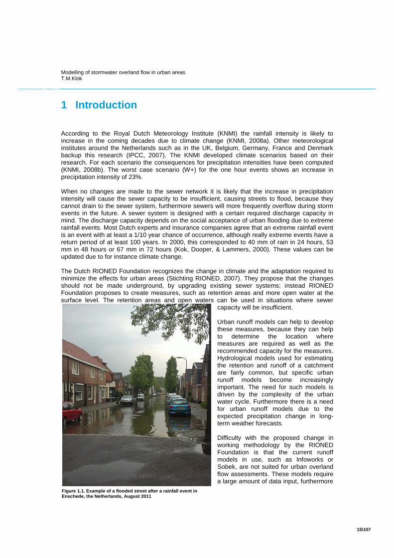
Figure 1.1. Example of a flooded street after a rainfall event in Enschede, the Netherlands, August 2011
Modelling of stormwater overland flow in urban areas T.M.Klok
16\107
the models are calibrated for average precipitation events, not extreme events. Such events demand different model structures.
1.1 Overland flow models In order to be able to perform overland flow assessments, alternative models have been developed. These models are called overland flow models. They are specifically designed to simulate extreme rainfall events. Overland flow models are mainly depended on a Digital Elevation Model (DEM), while „traditional‟ models, like Sobek depend on a linear representation of water streams. The advantage of a DEM is that water is allowed to flow in any direction in the model, instead of flowing through a preset network. There are different overland flow models available, for instance WOLK (WaterOverlast LandschapsKaart, from Tauw) and Wodan (Wateroverlast Oplossen door Driedimensionale Analyse, from Grontmij). The main difference between WOLK and Wodan is the flow routing methodology. This research will focus on WOLK. WOLK WOLK is a grid-based model which computes overland flow based on precipitation amounts and surface elevations. The purpose of WOLK is exploratory: to give an overview into overland flow routing and depression locations. The model is developed with the idea to use a minimal amount of input parameters, and produce relative accurate output. The surface elevations are described in a DEM, which are used to compute the flow direction of the surface runoff. The methodology of creating a DEM is subject to debate within Tauw. The surface elevations are also used to determine the location and size of depressions. Depressions are local depths in a surface grid, in which runoff can collect. After a preset amount of precipitation is distributed over the DEM, the depressions will collect some of the overland flow. By assessing each depression, the impact of the rainfall event can be determined. GIS applications allow for a visual presentation of the output data from WOLK. The visual presentation is useful for stakeholder sessions in which different approaches and measures for dealing with overland flow can be discussed. This application of WOLK has been proven to be useful in several cases, which had problems dealing with overland flow. In these projects however some limitations of WOLK emerged also. Some of the main drawbacks of WOLK were the flow routing and unknown time scale: it was unknown how much time has passed since the beginning of a rainfall event and the end situation computed by WOLK.
1.2 Research motivation As said before, some limitations of WOLK have become apparent during several cases. It is found necessary to further investigate these limitations. Furthermore, due to the low chance of occurrence of the precipitation events and the assumptions underlying WOLK, the accuracy of the model is uncertain. This research will focus on WOLK. Each aspect of the model will be reviewed: input data, limitations of the model, applicability of the model and the accuracy and relevance of the model output. Furthermore, in order to deal with the most urgent limitations, alternatives will be created and investigated. The research goal is: RESEARCH GOAL The goal of this research is to assess the accuracy and the limitations of WOLK and investigate alternative modelling procedures to complement for some of the limitations.

Modelling of stormwater overland flow in urban areas T.M.Klok
17\107
1.3 Research questions In order to establish the research goal a main research question and some sub questions have been formulated. The main research question is: MAIN RESEARCH QUESTION What are the strengths and limitations of WOLK and are there alternative methods to deal with these limitations? Sub-questions In order to answer the main question, the following research sub questions have been formulated. 1. Urban stormwater models In order to determine what the criteria are for a „good performing‟ overland flow model, the requirements from the user should be clarified. So the following questions are formulated:
1.1. Which processes are relevant in urban StormWater Management (SWM) during an extreme rainfall event?
1.2. What are the user requirements for an overland flow model? 1.3. What urban runoff models are available and how do these work?
2. Digital Elevation Model The Digital Elevation Model (DEM) has a substantial influence on the results of WOLK. In order to assess the performance of WOLK, an assessment of the influence of the DEM is required. The following questions are formulated to assess the influence of the DEM:
2.1. How does the DEM influence the output of WOLK? 2.2. Are there any issues related to the creation of a DEM for WOLK? 2.3. Which spatial interpolation techniques provide an accurate DEM?
3. Modelling Some issues related to WOLK, such as runtime, runoff routing and time dependency are known. A more extensive assessment of WOLK can reveal its strengths and weaknesses. The goal is to investigate alternatives for the limitations of WOLK. Therefore the following questions have been formulated:
3.1. What are the strengths and limitations of WOLK? 3.2. Which processes should be incorporated in WOLK in order to improve the
performance? 3.3. Are there alternative methods available to deal with the limitations of WOLK? 3.4. How do these alternatives influence the model results?
The interaction between sub-surface flow and overland flow can be complex and thus difficult to model and large amounts of data are required. Therefore the question stands:
3.5. Should WOLK deal with the interaction between sub-surface flow and overland flow and,if yes, how?

Modelling of stormwater overland flow in urban areas T.M.Klok
18\107
1.4 Methodology The methodology section will discuss how the research questions formulated in the previous section will be assessed. First, identification of relevant processes related to urban stormwater management, will be performed based on literature. The processes which are found relevant will be used to assess the input of WOLK later on. The relevancy also depends on the user requirements. The users of urban runoff models in the Netherlands are usually municipalities. The user requirements will be explored with interviews with Dutch municipalities. The user requirements will also be used to evaluate whether the purpose of WOLK is valid. Secondly, an assessment of available runoff models will be performed. This assessment will used to investigate whether the research has not already been conduced, or if there is something that can be learned from the found models. After that, a description of WOLK will be provided. The purpose is to get a thorough understanding of the model. The main limitations of WOLK will also be described here. The previous sections showed that the methodology for creating DEM files is inconsistent and therefore subject of debate. The quality of a DEM determines largely the results of overland flow computations in any model, thus a DEM should be as accurate as possible. The inconsistency in working method of creating a DEM will be assessed and a user guide will be developed which proposes a single methodology. Next, the proposed methodology in the user guide has to be evaluated. The user guide will therefore be used to execute WOLK for a case study. The case of Apeldoorn will be used. The assessment will be based on registered complains of overland flow and video/photo material from extreme rainfall events in the past. Video/photo material is used as an estimate of the accuracy of WOLK output. The assessment will give input for a SWOT analysis of WOLK. The SWOT analysis will show which limitations of WOLK should be used as a starting point for the development of alternative models. These alternative models will help determining if the original WOLK can and should be improved or not and which functions should be added then. WOLK is currently programmed in ArcGIS from ESRI. The use of ArcGIS brings advantages and limitations to the computation methodology. The use of Matlab is investigated as an alternative. One of the alternatives for WOLK will be a dynamic overland flow model. The dynamic model should be able to compute the dispersion of runoff through an urban area. An advantage of such an approach, compared to the ArcGIS method is that the results of WOLK will include more details, such as water heights and flow velocities. The alternatives will be tested in small idealized cases, to assess their performance and calibrate the models. After the alternative models are calibrated, they will be executed on several case areas. WOLK will also be executed for these cases. The results of alternative models will be compared that of WOLK. The comparison will be based on the differences in estimated waterlevels and flow routing computations between WOLK and the alternative models. The differences in estimated waterlevel will be computed with the use of ArcGIS, because of the spatial distribution of the WOLK output.
Modelling of stormwater overland flow in urban areas T.M.Klok
19\107
1.5 Report outline At first the field of urban stormwater management will be introduced in chapter 2. Furthermore the urban water cycle during extreme rainfall events is discussed, which gives insight into the relevant processes for modelling overland flow resulting from extreme rainfall events. A short review of the available models will show the difference between the more extensive urban runoff models and WOLK. Chapter 3 includes a description of WOLK. The known issues will also be described. Some issues that have been found related to WOLK are caused by different working methods within the Tauw organisation. Therefore in chapter 4 various alternatives for a user guide will be discussed. With the proposed user guide a WOLK has been executed. Chapter 5 shows the assessment of the results from the WOLK with the user guide and new data, which will be compared with a WOLK case from 2009 for the same area. The assessment will show the strengths, weaknesses, opportunities and limitations of WOLK. Based on the SWOT two alternative models have been in chapter 6. The alternatives are tested against previous WOLK cases in chapter 7. The assessment in this chapter shows whether the alternatives are valid improvements for WOLK. Chapter 8 will finish with some conclusions and recommendations.


Urban Stormwater Management
2
Use of models in urban stormwater management (SWM)


Modelling of stormwater overland flow in urban areas T.M.Klok
23\107
2 Urban Stormwater Management
Urban stormwater is defined as runoff from urban areas. Many factors influence the amount of stormwater, including: duration and intensity of rainfall, proportion of impervious surfaces, shape of the land, landuse and design & management of stormwater systems. Identifying treats and employ measures to counteract them is part of urban stormwater management. Large stormwater flows can cause sudden discharges from flooded sewer. Where properties are regularly affected, flood mitigation works have been constructed. Alternatively, the properties have been resumed and buildings demolished to create open space for recreation and use as flood detention basins. Increases in stormwater runoff volumes have resulted from increasing urbanization and the accompanying growth of impervious surfaces. Effective planning of flow paths across urban areas can reduce the speed and increase infiltration of stormwater runoff. Minimising the runoff from frequent storm events minimises sediment runoff and sewage overflows. The optimum solution for managing an increased volume of runoff is to encourage infiltration, storage and reuse.
2.1 Urban water cycle The processes in an urban water system are part of the water cycle. The difference between urbanized areas and natural areas is mainly the land cover type. Land cover affects the partitioning of water on that specific area. Urban areas partly consist of surfaces which are impermeable for water. These surfaces have a very slow infiltration rate and therefore generate more runoff compared to natural areas. Surface runoff can occur when a large enough amount of precipitation reaches the ground. In general precipitation can fall onto three types of surfaces: open water, permeable surface and impermeable surface. In most cities urban runoff is collected by (storm) sewer systems. Waste water from households is also collected by the sewer system. Sewer systems than transport the collected runoff and household wastewater to a waste water treatment plant (WWTP). In this example a combined sewer system is used. Other sewer systems include separated and improved separated systems, but for the purpose of explaining the relevant hydrology and hydraulic processes in urban water systems a combined sewer is used, because such a system includes all relevant processes. An overview of the relevant processes is given in Figure 2.1.

Modelling of stormwater overland flow in urban areas T.M.Klok
24\107
Figure 2.1. Overview of the relevant processes in an urban water system. Based on Shaw et al., 2011; Van Beek & Loucks, 2005; Noordhoff Atlasproducties, 2010
In the following sections the processes as shown in Figure 2.1 will be discussed, starting with precipitation, followed by infiltration and evaporation. After overland flow is formed the roughness becomes relevant as well as the routing of the runoff. Some of the runoff will flow into the sewers. Sewers can overflow, which also generates overland flow; therefore the processes around a sewer system will also be discussed. 2.1.1 Precipitation The effect of a rainfall event is based on two parameters, namely the intensity of rainfall, so the amount of precipitation in a given time period and the duration of the event. The definition of an extreme rainfall event is not stated clearly in literature. In the Netherlands the KNMI uses the following definition: 25 mm or more precipitation within one hour and/or at least 10 mm within 5 minutes (KNMI, 2008b). Such an event has a chance of occurrence of about once every ten years in the Netherlands. These statistics may change as a consequence of climate change. Table 2.1. Influence of KNMI climate scenarios on precipitation levels for several return periods. Klein Tank & Lenderink (2009).
Rainfall intensity
mm /hour mm/day
Return period Current G G+ W W+ Current G G+ W W+
1 year 14 15 15 17 17 33 36 35 39 36
10 years 27 30 30 33 33 54 60 57 66 60
100 years 43 48 48 53 53 79 80 84 84 88
The KNMI developed climate scenarios to predict the change in precipitation in the future. Four scenarios have been developed: G-scenario: is the most average scenario. It assumes 1 °C temperature increase on earth in the period 1990-2050. W-scenario: is the most average scenario. It assumes 2 °C temperature increase on earth in the period 1990-2050. + indicates that also a change in air flows is assumed with milder and wetter winters and wetter, while summers will be warmer and dryer.

Modelling of stormwater overland flow in urban areas T.M.Klok
25\107
The results of the scenarios in table 2.1 show that the predictions have a range, corresponding to a level of certainty of the predictions. The increase in precipitation intensity can be used to simulate the urban drainage system and overland flow in order to assess whether the system is robust enough to deal with the predictions of the KNMI. For modelling purposes the upper boundaries of the predictions can be used as a worst case scenario. 2.1.2 Infiltration An issue with infiltration is that measurements during extreme rainfall events in the Netherlands are almost none existent. Therefore a variety of modelling methods is proposed (Klok, 2011). In modelling practises infiltration is simulated with different methods, depending on the scale and purpose of the model. At, catchment scale, infiltration is sometimes used as a balancing parameter for the water balance (Van Beek & Loucks, 2005). A method that is similar to the balancing principle is modelling the infiltration by a runoff coefficient. A runoff coefficient is a ratio of surface runoff to rainfall. An alternative approach is to use information about the soil structure to estimate the saturated hydraulic conductivity. In practise this method will not work, because the hydraulic conductivity during extreme precipitation events is unknown. The easiest method for incorporating infiltration in urban overland flow modelling is describing infiltration as a percentage of the total amount of precipitation. 2.1.3 Evaporation In this research the focus is on modelling runoff during and just after storm water events. Mark et al. (2004) concluded that evaporation is insignificant for the simulation of maximum flood depths due to storm events. They found that evaporation per unit city area was approximately 0.5% of an accumulated precipitation event for Dhaka city in Bangladesh. Van Beek and Loucks (2005) as well as Grayson & Blöschl (2000) conclude that models designed to simulate storm runoff from particular rainfall events may safely ignore evaporation. Therefore during this research the amount of evapotranspiration is therefore assumed to be negligible during heavy rainfall events. 2.1.4 Sewer system A combined sewer system is also used to transport runoff from precipitation events. During extreme rainfall events sewers may become saturated. The excess amount of runoff will then become overland flow. It is unknown whether or not this behaviour is significant for overland flow modelling. It is therefore unknown if sewer flow should be incorporated in urban runoff modelling. Sewer flow can be modelled in different ways. The research found in the literature review (Klok, 2011) showed that sewer systems are often modelled as one dimensional flows (Hsu et al., 2000; Mark et al., 2004; Leandro et al., 2009). A difficulty with modelling is that discharge through a gravity pipe can either be free-surface when flow is below conduit capacity or supercritical when wastewater and/or stormwater are under pressure within a gravity drain. The reviewed articles all used some sort of derivation from the St. Venant equations (Appendix C). Most models use the St. Venant equations in some simplified form. In the simplifications processes like friction, evaporation, etc are not included. The description of sewer system modelling shows that such a model is complex in itself even when simplifications are used. In combination with an overland flow model the model would become even more complex. Moreover, because the sewer system is fully saturated during extreme events its need for complex modelling is decreased. Only at the beginning of and after the storm a detailed sewer model is expected to be relevant. Therefore the sewer system is included in the model as a single parameter. The parameter represents the maximum amount of discharge that the sewer system is designed for; the sewer system is thus assumed to be fully saturated. Any exchange of runoff between the sewer system and the overland flow will be ignored. This assumption means that sewer overflows are neglected.

Modelling of stormwater overland flow in urban areas T.M.Klok
26\107
2.1.5 Overland flow The term „overland flow‟ refers to the flow of water over a surface. Overland flow can be generated in two ways. First, it is generated when the rainfall intensity exceeds the surface infiltration capacity. This capacity depends on the soil characteristics as well as the surface slope. The excess rainfall then accumulates on the soil surface in small depressions. Once these depressions are filled, the water spills out and flows downslope as overland flow. Overland flow originating in this way is called Horton overland flow (Grayson & Blöschl, 2000). Overland flow is also generated when a rising water table intersects the soil surface, which means that the soil is fully saturated. This process is called seepage. Seepage then exits from the soil and becomes overland flow. Seepage is neglected in this research, because the time scale in which it occurs is significant larger compared to overland flow directly resulting from precipitation.
2.2 Urban stormwater models Overland flow is a portion of the total amount of runoff. The other part is sewer runoff, see also figure 2.2. Since the 1950s hydrologic models have been developed, which were used to calculate quantities of runoff, primarily for riverine flood forecasting. Today the focus is broadened to overland flow modelling of in urban areas also. There are several models available that can be used to simulate urban surface runoff with the use of a Digital Elevation Model (DEM). WOLK is an example of such a model. An overview of similar grid-based models that are available on the market is presented in Appendix A. Two examples of software packages that can simulate overland flow as well as sewer and
open water flows, are Sobek and Infoworks. Both these models are commonly used in the Netherlands. Sobek is developed to be used for flood forecasting as well as the simulation of drainage systems, irrigation systems, river morphology, salt intrusion and water quality. Infoworks on the other hand has been developed for the simulation of sewer systems, including the simulation of sewer overflow, sedimentation and water quality. Although both these software products use validated overland flow models, they are not used at Tauw for overland flow simulations. This is because the required extensions of overland flow are not cheap (which is important from a company point of view). Furthermore, in order to run these sophisticated models properly, they require lots of detailed inputTable 2.2 gives an overview of the required data input. The table only includes models which are available at Tauw.
Overland flow
Sewer runoff
Pre
cip
itat
ion
Infi
ltra
tio
n
RunoffSoil surface
Figure 2.2. Division and terminology of water after a precipitation event (Van Beek & Loucks, 2005).
Modelling of stormwater overland flow in urban areas T.M.Klok
27\107
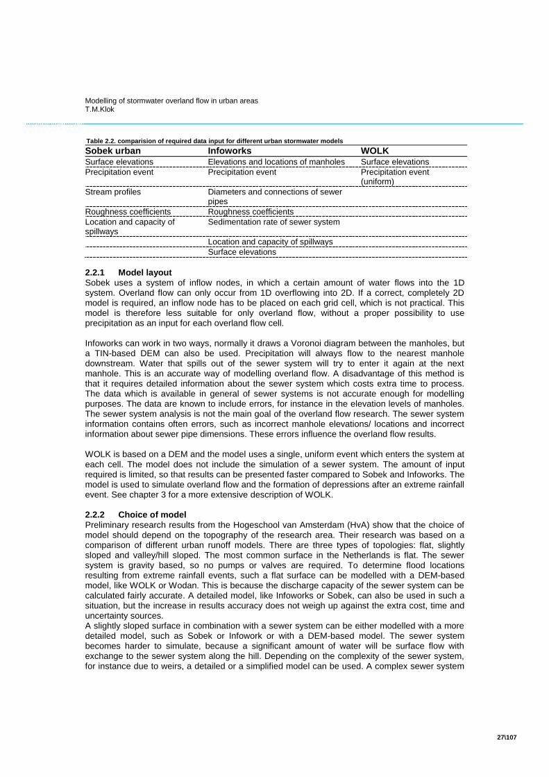
Table 2.2. comparision of required data input for different urban stormwater models
Sobek urban Infoworks WOLK Surface elevations Elevations and locations of manholes Surface elevations
Precipitation event Precipitation event Precipitation event (uniform)
Stream profiles Diameters and connections of sewer pipes
Roughness coefficients Roughness coefficients
Location and capacity of spillways
Sedimentation rate of sewer system
Location and capacity of spillways
Surface elevations
2.2.1 Model layout Sobek uses a system of inflow nodes, in which a certain amount of water flows into the 1D system. Overland flow can only occur from 1D overflowing into 2D. If a correct, completely 2D model is required, an inflow node has to be placed on each grid cell, which is not practical. This model is therefore less suitable for only overland flow, without a proper possibility to use precipitation as an input for each overland flow cell. Infoworks can work in two ways, normally it draws a Voronoi diagram between the manholes, but a TIN-based DEM can also be used. Precipitation will always flow to the nearest manhole downstream. Water that spills out of the sewer system will try to enter it again at the next manhole. This is an accurate way of modelling overland flow. A disadvantage of this method is that it requires detailed information about the sewer system which costs extra time to process. The data which is available in general of sewer systems is not accurate enough for modelling purposes. The data are known to include errors, for instance in the elevation levels of manholes. The sewer system analysis is not the main goal of the overland flow research. The sewer system information contains often errors, such as incorrect manhole elevations/ locations and incorrect information about sewer pipe dimensions. These errors influence the overland flow results. WOLK is based on a DEM and the model uses a single, uniform event which enters the system at each cell. The model does not include the simulation of a sewer system. The amount of input required is limited, so that results can be presented faster compared to Sobek and Infoworks. The model is used to simulate overland flow and the formation of depressions after an extreme rainfall event. See chapter 3 for a more extensive description of WOLK. 2.2.2 Choice of model Preliminary research results from the Hogeschool van Amsterdam (HvA) show that the choice of model should depend on the topography of the research area. Their research was based on a comparison of different urban runoff models. There are three types of topologies: flat, slightly sloped and valley/hill sloped. The most common surface in the Netherlands is flat. The sewer system is gravity based, so no pumps or valves are required. To determine flood locations resulting from extreme rainfall events, such a flat surface can be modelled with a DEM-based model, like WOLK or Wodan. This is because the discharge capacity of the sewer system can be calculated fairly accurate. A detailed model, like Infoworks or Sobek, can also be used in such a situation, but the increase in results accuracy does not weigh up against the extra cost, time and uncertainty sources. A slightly sloped surface in combination with a sewer system can be either modelled with a more detailed model, such as Sobek or Infowork or with a DEM-based model. The sewer system becomes harder to simulate, because a significant amount of water will be surface flow with exchange to the sewer system along the hill. Depending on the complexity of the sewer system, for instance due to weirs, a detailed or a simplified model can be used. A complex sewer system

Modelling of stormwater overland flow in urban areas T.M.Klok
28\107
is harder to capture in a single parameter for the whole research area. This results in the need for detailed models. The last surface type is a valley or hill shaped. Runoff will concentrate in the centre of the valley and disperse away from the top of the hill. This type of surface is best modelled with DEM-based models. If a sewer system exists, it is more likely to overflow in a valley than on top of a hill, so the flood location is similar to the depression location. Therefore the simulation of a sewer system will not significantly influence the results.
2.3 User demands A practical issue with models is that they are normally developed with a purpose and a user-group in mind. Some models have been developed specifically for modelling extreme rainfall events in urban areas. The user-group or client in this case is municipalities. Municipalities in the Netherlands are by law responsible for the collection and transportation of sewage. They are also responsible for the construction and maintenance of the sewer system and any problems caused by extreme rainfall. In order to understand what the demands are of the user-group in relation to urban runoff models, interview sessions have been set up as part of this research. The interviews have provided insight into the expectations of the user-group as well as their determinants for a useful model. For this research three representatives from the municipalities of Apeldoorn, Deventer and Eindhoven have been interviewed. These municipalities have been selected because they have had WOLK being executed recently for their municipality. An overview of the interview questions can be found in Appendix B. The interviews showed that in general municipalities are cautious with model output. They tend to rely more on expert knowledge of the area they are responsible for. An example given by a municipality of the use of expert knowledge was the determination of the location and size of a retention basin. Such a basin is used to collect an excess amount of precipitation. The location and the dimensions of the basin are determined by roughly estimating where a large amount of water flows and then estimating the upstream area. The upstream area times the precipitation amount determines the required retention capacity. The determination of the upstream area in urban environments is arbitrary, because of the complexity of the system. A model can help municipalities to compute the upstream area more easily and more accurate. The interviews showed that municipalities do not always want to use this option. The decision of using runoff models depends on the personal preference of the municipal representatives. From the interviews some general user demands can be determined. First of all, a model should not be a „black box‟. Municipality representatives should be able to understand the processes in the model. Secondly, the results of the model should be meaningful and usable. Although the interviews showed that each municipality has a different view on what is meaningful. 2.3.1 Consequences of floods The interviews revealed that some municipalities expect from models that they add something else. With the use of models not only the quantity of runoff can be simulated, but also the consequences of the runoff in the form of damage. Damage is a broad concept. Mark et al., (2004) and Kok et al., (2006) divided damage from urban floods into two categories: 1. Direct damage, this is mostly material damage caused by inundation and/or flowing water. 2. Indirect damage, this damage originates from the secondary effects of a flooding, such as
diseases and production losses of companies. The table below categorizes different types of damage into direct and indirect damage. Damage with an economic value are the easiest to calculate after a flood (or any other disaster) has

Modelling of stormwater overland flow in urban areas T.M.Klok
29\107
occurred. Damage which cannot be prized is also categorized, because this is also relevant for flood damage estimations. A more detailed description of the types above can be found in the report of Kok et al. (2006). This thesis will not discuss flood damage, because for an accurate computation of flood damage, the flood itself should be modelled more accurately. Table 2.3. Flood damage categories and examples for each category.
Damage Prized (monetary) Unprized
Direct Buildings Furniture Vehicles Capital goods Crops Infrastructure Company production loss (within flooded area) Dikes and weirs Evacuation and aid
Casualties Injured Animal casualties Social consequences Disruption of normal transport modes Public facilities out of service Communications resources out of service Cultural-historical objects Landscape, nature and environment Legal actions
Indirect Market disruption (outside flooded area) production losses of companies (outside
flooded area) Temporary housing Medical aid on long term
Society disruption Market disruption Damage for government Social consequences
The municipalities of Deventer and Apeldoorn are not interested in estimating damage risk caused by extreme rainfall events. Only the Eindhoven municipality is interested in damage estimations. Deventer and Apeldoorn argue that they do not suffer the consequences of damage. Instead claims are being paid by insurance companies. Both the municipalities of Deventer and Apeldoorn have the policy that in general they try to minimize inconvenience for inhabitants due to extreme rainfall. When inhabitants complain a lot, they get a higher priority. On the other side it is positive that municipalities distrust models, because that means that they will review model output critically. The downside is that municipalities will not explore the possibilities of models, because they distrust models in general.
2.4 Conclusions Stormwater management in the Netherlands is becoming increasingly important. The introduction discussed the climate scenarios developed by the KNMI. These climate scenarios make the field of urban stormwater management interesting, due to the high level of impermeable surfaces. Impermeable surfaces, such as buildings and roads, prevent water to infiltrate into the subsoil. The use of combined sewer systems in the Netherlands adds to the complexity of urban stormwater management. The choices made in the analysis of the relevant processes have been based with the purpose of WOLK in mind. The purpose of WOLK is exploratory; the model is developed with the idea to use a minimal amount of input parameters, and produce relative accurate output. The relevant processes for modelling overland flow have been found to be at least: the amount of precipitation and the surface elevation, although more accurate results can be produced when the surface type and infiltration are also included. More complex models include more processes, but this not always leads to more accurate results, because the interactions of these processes are not always clear. Furthermore the limited amount of data and other information which is available can be an issue. The users of overland flow models are municipalities. They are sceptical towards the use of such models, because they tend to rely more on expert knowledge. Therefore overland flow models are only useful when they add to the expert knowledge, and not try to replace the experts. In this way a model can be made which will be used by the user group it is intended for.


WOLK
3


Modelling of stormwater overland flow in urban areas T.M.Klok
33\107
3 WOLK


Towards a uniform use of WOLK
4
WOLK Guide

Modelling of stormwater overland flow in urban areas T.M.Klok
37\107
4 Towards a uniform use of WOLK
The previous chapter discussed the issues related to WOLK
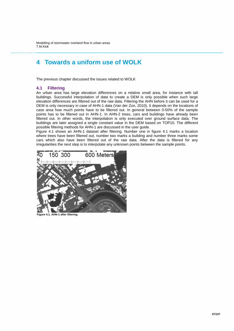
4.1 Filtering An urban area has large elevation differences on a relative small area, for instance with tall buildings. Successful interpolation of data to create a DEM is only possible when such large elevation differences are filtered out of the raw data. Filtering the AHN before it can be used for a DEM is only necessary in case of AHN-1 data (Van der Zon, 2010). It depends on the locations of case area how much points have to be filtered out. In general between 0-50% of the sample points has to be filtered out in AHN-1. In AHN-2 trees, cars and buildings have already been filtered out. In other words, the interpolation is only executed over ground surface data. The buildings are later assigned a single constant value in the DEM based on TOP10. The different possible filtering methods for AHN-1 are discussed in the user guide. Figure 4.1 shows an AHN-1 dataset after filtering. Number one in figure 4.1 marks a location where trees have been filtered out, number two marks a building and number three marks some cars which also have been filtered out of the raw data. After the data is filtered for any irregularities the next step is to interpolate any unknown points between the sample points.
Figure 4.1. AHN-1 after filtering.
1
2
3

Modelling of stormwater overland flow in urban areas T.M.Klok
38\107
4.2 Spatial interpolation ArcGIS provides several interpolation methods for spatial data. Below four interpolation methods will be discussed. The interpolation methods available in ArcGIS are: Spline, Natural Neighbor (NN), Inverse Distance Weighting (IDW) and Kriging. Each method will shortly be described and assessed on its usability for the purpose of DEM preparation. 4.2.1 Spline Spline interpolation connects sample points with a smooth continuous plane. A mathematical spline is constrained at the sample points, but between the points it flexes in a manner that results in a smoothly varying plane. Splines are not analytical nor statistical models. They are arbitrairy and devoid any theoretical basis (Davis, 2002). However they can be useful to interpolate surfaces quickly. The general Spline equation which is used in ArcGIS can be written as
(2.1)
Where: = spline surface
= 1, 2, …, n = number of sample points
= coefficients found by the solution of a system of linear equations
= the distance from point to the th point.
and are defined differently, depending on a selected option in ArcGIS. There are two
available options: regularized and tension.
For the regularized option and are defined as follows:
(2.2)
(2.3)
Where: and are the parameters entered at the command line in ArcGIS.
the Bessel function, see (Davis, 2002).
a constant equal to 0.577215.
= coefficients found by the solution of a system of linear equations.
For the tension option and are defined as follows:
(2.4)
(2.5)
Spline is not suitable for urban areas, because of the large spatial variability unless many sample points are available. This may be the case with AHN2 laser points, but this has not been tested. Furthermore, spline interpolation has the possibility to produce unusable results for a DEM. Therefore spline interpolation will not be used for further research.

Modelling of stormwater overland flow in urban areas T.M.Klok
39\107
4.2.2 Natural Neighbor Natural Neighbor (NN) interpolation finds for an unknown point several nearby known sample points and applies weights to them based. The weights are based on the proportionate areas of the known sample points (Davis, 2002). The areas around the sample points are determined by constructing Thiessen polygons. Initially a Thiessen diagram is constructed from all the sample points. When the unknown point is introduced a new Voronoi is drawn. The proportion of overlap between this new polygon and the initial polygons are then used as weights.
Figure 4.2.a. Voronoi diagram before introducing unknown point
Figure 4.2.b. Voronoi diagram after introducing unknown point. The value of the new point is based upon the value overlaping with the old polygons
The basic properties of NN are that it searches only local, furthermore the interpolated value will always stay within the range of the sampled data used, which is different from for instance the Inverse Distance Weighting. NN does not influence trends in the data nor does it introduce peaks, pits, ridges, etc. The interpolated surface with NN is a smooth surface except at the locations of the sample points (see figure 4.5). A disadvantage of NN is the possibility of clusters of sample points which can occur. These points are likely to have about the same value. The new value will therefore also likely have a value close to the grouped sample points average. A possibility to correct for such clustering is the use of Inverse Distance Weighting (IDW). Although in the case of WOLK, this is not really necessary, because the unknown point lie in a regular spaced grid. An issue with NN in ArcGIS is that it requires a significant amount of computer virtual memory (RAM). This is because for each sample point and Thiessen polygon the specifications have to be stored. Therefore, depending on the computer specifications, a maximum amount of sample points can be used as input for NN.
34
22
34
30
33
34
22
34
30
33

Modelling of stormwater overland flow in urban areas T.M.Klok
40\107
4.2.3 Inverse Distance Weighting Inverse Distance Weighting (IDW) is based on the principle that known points closer to an unknown point will predict the value at a new location better, compared to points which are further away. Therefore IDW assigns weights to each sample point relative to the unknown point. The larger a weight is, the more important a point is in predicting the unknown value. The standard weight function for IDW is:
(2.6)
Where is distance between a point and the unknown point. The power in function 2.6
represents the weighting function used in IDW. The weights that are assigned to the sample points according to the weighting function are adjusted to sum up to 1.0 (Davis, 2002). Therefore, the weighting function actually assigns proportionally weights and expresses the relative influence of each sample point on the unknown point.
Figure 4.3. IDW example layout
Figure 4.4. Effect of the power function in IDW, based on equation 2.6.
The value for the unknown point will be:
(2.7)
Where is the elevation value for the new point. An example of IDW, based on figure 4.3, with
Power “2” is given below:
A disadvantage of IDW is that it can produce a “bulls eye”. These are local extreme variations in the map. Bulls eyes are caused by one deviant sample value close by, which get a high weighting according to IDW. The example in figure 4.5.C. shows the bulls-eye effect. Other interpolation methods are less influenced by local extreme variations in a map, because they either compensate for this effect (Kriging) or the effect is less because no weighting is used (NN).
1
34
22
342.5
2
3
4
30
33
0
0.2
0.4
0.6
0.8
1
1 2 3
We
igh
t
Distance
Inverse Distance Weighting
1/D^1 1/D^2 1/D^3 1/D^4

Modelling of stormwater overland flow in urban areas T.M.Klok
41\107
4.2.4 Kriging Kriging is by far the most complicated interpolation technique. The principle of kriging is similar to IDW, in the sense that points that are closer by are assumed to have a higher correlation with the unknown point. But kriging also takes the correlation between the known points into account. In this way kriging corrects for spatial clustering in the sample points. In this way clusters of data, or the “bulls eye” effect of IDW are avoided. Only correlated sample points contribute to estimate at unvisited location. In order to do so the Standard Error of the kriging estimate at each grid node is computed (also called kriging estimation variance). The output is a map with interpolation uncertainty instead of a single value for the whole map. The kriging function is as follows:
(2.8)
Where, is the variable to be interpolated (in this case surface elevation).
= the estimated value of at the unvisited node
= the mean value of
= the kriging weight for the value of at the observation point
= the observed value of at the observation point = the total number of datapoints used in the estimation of at the unvisited node
The kriging weight is based on the semivariogram. The semivariogram includes a fitted model
through the sample points. The fitting is the most subjective part about kriging. There are multiple fitting methods possible, each resulting in different kriging maps (Davis, 2002). ArcGIS allows for the following fitting models: circular, spherical, exponential, gaussian and linear. It goes too far to explain each model and discuss the influences on the kriging results, but more information can be found in Davis (2002). The fitting of the models in a semivariogram requires expert knowledge of the method, furthermore kriging is a time consuming method. Kriging requires a large amount of computer power and memory. As a result of that the case area size has to be limited compared to the other interpolation methods. Smaller case areas are unwanted, because case borders can influence the overland flow. This issue is discussed in the user guide. Another issue with kriging is that the input data should not have trend in it. Thus, when kriging is used for areas at for instance a hillslope the trend in surface elevations has to be removed and later put back again. Based on all the disadvantages kriging is found not to be referenced for WOLK.
Modelling of stormwater overland flow in urban areas T.M.Klok
42\107
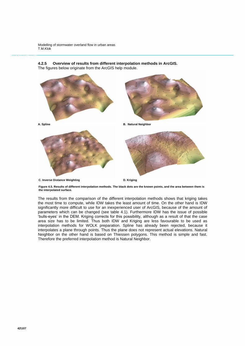
4.2.5 Overview of results from different interpolation methods in ArcGIS. The figures below originate from the ArcGIS help module.
A. Spline
B. Natural Neighbor
C. Inverse Distance Weighting
D. Kriging
Figure 4.5. Results of different interpolation methods. The black dots are the known points, and the area between them is the interpolated surface.
The results from the comparison of the different interpolation methods shows that kriging takes the most time to compute, while IDW takes the least amount of time. On the other hand is IDW significantly more difficult to use for an inexperienced user of ArcGIS, because of the amount of parameters which can be changed (see table 4.1). Furthermore IDW has the issue of possible „bulls-eyes‟ in the DEM. Kriging corrects for this possibility, although as a result of that the case area size has to be limited. Thus both IDW and Kriging are less favourable to be used as interpolation methods for WOLK preparation. Spline has already been rejected, because it interpolates a plane through points. Thus the plane does not represent actual elevations. Natural Neighbor on the other hand is based on Thiessen polygons. This method is simple and fast. Therefore the preferred interpolation method is Natural Neighbor.

Modelling of stormwater overland flow in urban areas T.M.Klok
43\107
Table 4.1. Overview of run time for various interpolation methods in ArcGIS. The same computer is used for all computations.
Interpolation method
Raster size (cells)
power Search method
search radius (m)
method Semivariogram model
Runtime (hh:mm:ss)
Spline 0.5 mln regularized 00:04:15
NN 0.5 mln 00:01:20
0.5 mln 00:06:21
1 mln 00:16:18
IDW 2 mln 2 fixed 1250 00:03:57
0.5 mln 3 fixed 5 00:02:31
0.5 mln 1 fixed 4 00:02:29
0.5 mln 3 variable 12 points, max 10m
00:03:30
1 mln 1 fixed 24 00:14:02
Kriging 0.5 mln ordinary spherical 04:54:28
The above interpolations methods are ArcGIS based. Spatial interpolations can also executed within other software environment. The interpolation techniques will not change, the only thing that might be changed is the effectiveness of the data handling. This might result in less runtime for the spatial interpolations. This option has not been investigated during this research, because the interpolation is a relative small step in the total process. Therefore the amount of runtime which can be gained from it is not significant enough at the moment. As a result of that, interpolation will be executed with ArcGIS.
4.3 Raster cell size Cell size is a discussion point with models in general, and WOLK is no exception. The cell size has an influence on the accuracy of the model. The flow routing is likely to vary depending on the raster size.
A. Grid size: 0.5 meter
B. Grid size: 1.0 meter
C. Grid size: 2.0 meter
Figure 4.6. Effects of different cell sizes on the accuracy of a DEM. Dark grey is low elevation, light grey is high elevation. White is unknown elevation (NoData). (1) are filtered out buildings and (2) are filtered out cars.
The above maps show differences between different cell sizes for urban areas. The maps show a street and buildings and parked cars on either side. The road is raised in the middle. Selecting a correct cell size is more important for urban areas than rural areas, because the spatial variability is larger. In urban areas, there are several small obstacles, such as road bumps, sidewalks and fences, which influence the flow of water. Especially when a cell size of 2x2 meter or larger is chosen the maps becomes distorted. A connection between two adjacent buildings in the 0.5x0.5 and 1x1 meter map is lost in the 2x2 meter map. Furthermore small details are lost. Such losses in detail can be significant in the case of flood routing. Water can flow in a different direction than is possible in reality, resulting in incorrect model output. On the other hand is a larger grid size an advantage on data handling, because if the number of cells in a grid decreases the process time also decreases. The choice for a grid size is a trade-off between accuracy and data handling. In the case of WOLK the level of detail requires at least a raster size of 1x1 meter, some test runs show that a more detailed raster size does not add much
2
1
1

Modelling of stormwater overland flow in urban areas T.M.Klok
44\107
accuracy to the results. This can also be explained by the obstacles in an urban area. Significant obstacles such as alleys or pathways are mostly larger than 1x1 meter, and thus will be visible. Fewtrell et al. (2008) arrive at the same conclusion. They suggest that model resolutions up to the characteristic length of buildings size and street width provide consistent and sufficiently accurate predictions of flooding. Although they use their model to simulate the effects of floods in urban areas, instead of overland flows, their observations are considered to be valid. Therefore the optimal raster size is chosen to be 1x1 meter.
4.4 Conclusions The assessment of spatial interpolation methods available in ArcGIS has shown that Natural Neighbor is the most preferable interpolation technique, mostly because it is the most user friendly technique. NN excludes as much human error by keeping the amount of parameters to the minimum. The choice of raster size is a trade-off between model accuracy and data handling. The level of trade-off is based on expert opinion. The break-even point is a raster size of 1x1 meter. Model accuracy is more important than data handling, but data handling is constrained by the available computational power available on the market.

Assessment of WOLK
5
An alternative approach to overland flow modelling


Modelling of stormwater overland flow in urban areas T.M.Klok
47\107
5 Assessment of WOLK
The user guide, which has been developed in the previous chapter, has been used to prepare the DEM for WOLK for the case of Apeldoorn. This case is used to assess the performance of WOLK by comparing the results of the model with recorded floods in Apeldoorn. Furthermore, the influence of a DEM on the results is assessed. The case of Apeldoorn has been chosen, because this case was available from Tauw and evaluated before.
5.1 Case description Apeldoorn is located in the centre of the Netherlands (figure 5.1) on some very gentle hill slopes and had about 136,600 inhabitants in 2009. Tauw was asked by the municipality of Apeldoorn to assess the overland flow problems in the city after a heavy rainfall event in 2009. In order to do so Tauw used WOLK to compute the inundation areas in the city based on the surface level, runoff routes and retention areas for the runoff. The surface levels were extracted from the Actueel Hoogtebestand Nederland (AHN-1) (Van der Zon, 2010).
Model changes The initial results of WOLK 2009 were not in line with the eyewitness statements from the rainfall event. This proves that the model results are not accurately simulating the consequences of the rainfall event. A discrepancy between model results and reality demands an assessment of the causes of these differences. During the project the conclusion was that the overland flow at several locations was estimated incorrectly. Thus either the runoff routing or the DEM were incorrect. The output has been discussed in guided sessions by Tauw with people from the municipal departments of water and sewer, transport, spatial planning and environment. Their recommendations as how to deal with problematic areas were used to make changes to the DEM and recalculate the case as well as the measures against floods. The result of this process was the selection of measures adapted specifically to minimize the direct damage of overland flow. In April 2011 a new AHN became available. The AHN-2 was measured in
2010, so the DEM is a relative accurate representation of current reality, because in Apeldoorn no large building projects are executed between 2010 and 2011. The difference with AHN-1, which is five years older, is that the new AHN has a higher density of sample points (Van der Zon, 2010). Furthermore, the vertical accuracy has also improved; see also the user guide for more information.
Figure 5.1. Research locations 1 and 2 marked on the map of Apeldoorn. Black lines represent the borders of case areas, red lines represent significant flood locations.

Modelling of stormwater overland flow in urban areas T.M.Klok
48\107
The renewed DEM was a reason to execute WOLK again for Apeldoorn. A disadvantage of the AHN-2 was that the process steps related to the preparation of the WOLK input data had to be redefined, due to the increase in data size. This has been described in the WOLK guideline in the previous section. The ArcGIS version in both the 2009 and 2011 case are the same, namely ArcGIS 9.2. WOLK 2011 uses newer data versions of the AHN, Infoworks (sewer) computations and land use (TOP10). The Infoworks results are used to evaluate the performance of WOLK. The surface usage is used to determine the locations of impermeable surfaces. The extreme event which is modelled remains 60 mm in one hour, where 40 mm becomes surface runoff. Furthermore, the grid size remains 1x1m for the WOLK computations. The largest difference between the two data versions, is that the 2009 version had to be filtered for trees, buildings, cars, etc. The remaining data was then interpolated with Natural Neighbor. The 2011 version based on AHN-2 data has more data points left after filtering, compared to the AHN-1 DEM. Therefore it is expected that the AHN-2 DEM will be more accurate than the AHN-1 DEM. For the 2011 version of the model new data of impermeable surfaces was used. The total area of impermeable surface has increased since 2009. Although for the analysis an area was chosen where the change in impermeable surface is minimal. Table 5.1. Differences and similarities between WOLK 2009 and WOLK 2011
WOLK 2009 WOLK 2011
Similarities
ArcGIS 9.2
60 mm of precipitation
Grid cell size
WOLK version
Differences
AHN-1 AHN-2
Impermeable surface 2009 Impermeable surface 2011
Tauw filtering method for AHN AHN already filtered
Sewer model 2009 Sewer model 2011
DEM based on IDW DEM prepared according to user guide
5.2 Comparison of WOLK ‘09 and ‘11 Based on the results of the stakeholder session of WOLK 2009, some locations have been selected, where the results of WOLK 2011 have been compared with the results of WOLK 2009. The locations are chosen based on the amount of predicted flooding and the amount of available data known by municipalities, such as photo and film material for confirmation. These locations are shown in figure 5.1. The results of both WOLK 2009 and 2011 are shown in figure 5.2 and 5.3. The results of WOLK 2009 and 2011 are similar, which was according to expectations. The DEM is not changed radically; therefore the larger depressions are the same. Furthermore there were no large land use changes in the observed period. Another similarity between WOLK 2009 and 2011 is the runtime. The runtime has been experienced as too large for WOLK to be usable in live stakeholder sessions, although for desk studies the runtime is well within acceptable ranges.. In an ideal situation WOLK is able to run within a minutes, so that measures can be computed during stakeholder sessions. This has also been discussed in chapter three. Between the output of WOLK 2009 and WOLK 2011 for Apeldoorn there are some differences. In the 2009 version there are more small depressions which are filled with runoff. The 2011 version of WOLK on the other hand is „smoother‟, in the sense that runoff is collected in larger depressions. Therefore the flooding of certain roads in WOLK 2011 is even more overestimated than it already was with the 2009 results. The overestimation will be discussed in more detail later on. Another difference is that the 2011 version has longer flow lines, which means that water can discharge continuously for a longer amount of time compare to the 2009 version of WOLK. The longer flow lines are partly caused by the overestimation and partly because the AHN-2 DEM is smoother, thus increasing the possibilities for overland flow to continue flowing. The flow lines

Modelling of stormwater overland flow in urban areas T.M.Klok
49\107
represent the runoff routing of overland flow. In figure 5.3 this is shown in the results as a dark blue flow path line. The longer flow lines are not realistic. In reality the flows are not as concentrated as computed by WOLK 2011, because overland flow is not likely to flow several kilometres in urban areas; instead it will discharge into the sewer system, infiltrate or reach a pond much sooner. Furthermore, water will disperse over a larger area. Overland flow in WOLK discharges only to the lowest adjacent raster cell, causing the concentrated flow. This behaviour of WOLK is a downside to the model, because when measures are developed, people cannot rely on the flow lines estimated by WOLK. Expert knowledge about the area remains necessary. When zooming in on specific locations within the area, the areas with a significant amount of flooding or overland flow have been marked with red circles. The upper dark red circle in the figures 5.2 and 5.3 indicates an area where flooding of basements has been reported by inhabitants after the rainfall event in 2009. In both the 2009 and 2011 version of WOLK the cause for these floods is not obvious. Therefore the assessment is not limited to inundation and flow lines, but the DEM is also used. The WOLK 2011 DEM for this area can be found in Appendix D. The inundated area on the north side near the buildings is a local depression. The precipitation has therefore no option other than to flow into the basements of the houses. WOLK 2009 results are more extreme than the 2011 version around the basements: the depressions are larger, especially around the most northern building inside the dark red circle. In the 2011 version an explanation might be found in the flow lines. A large flow path runs just aside of the flooded buildings, which would take up some of the overland flow, resulting in less inundation around the flooded buildings. The light red circle and the black dotted line mark areas where reports are filed concerning water on streets after the rainfall event in 2009. In both locations the estimated flood is worse in the 2011 version of WOLK. The area and depth of the floods is larger compared to the WOLK 2009 results. Two movies, shot by inhabitants, show a flood depth of up to one to two decimetres of water on the streets. The locations of the movies are marked in figures 5.2 and 5.3 by the black dotted line. The flood depth is estimated from the cars which run through the street; furthermore the walkways are completely flooded. Both WOLK 2009 and 2011 results show a flood depth of 4 to 7 decimetres. Caution is required, because the rainfall event in 2009 has occurred under different conditions than modelled here. The total amount of precipitation in the 2009 rainfall event was about 115 mm of rain in one and a half hour, which has a chance of occurance of less than once every 100 years. WOLK simulates an event of 60 mm which falls instantly. Still, the results of WOLK overestimate the amount of flooding. This is a known error of WOLK and is likely caused by the fact the sewer system is excluded from the model. The coloured dots are Infoworks CS results, which have been calculated independently of WOLK. The blue dots in the area show that there is sewer capacity left on these locations. Runoff will discharge into the sewer system on these locations. Orange dots are the opposite; there water will flow out of the sewer into the streets. For these computations a standardized Dutch rainfall event (bui10) was used. This is a precipitation event with a return period of 10 years, which is considerably less than the 100 year return period which is used as input for WOLK. Infoworks CS computations using rainfall events with larger return periods has no use, because as soon as the sewer system overflows, the model results become too uncertain. The uncertainty is caused by the overland flow, which is not incorporated in Infoworks CS. This has been discussed in chapter 2 of this report. At the locations where WOLK estimated floods, the orange dots show there is a shortage of capacity. The waterlevel is estimated by Infoworks to be 2 to 5 decimetres above the surface, which is thus in line with the WOLK results. The results of WOLK 2009, 2011 and Infoworks CS show the locations of floods correctly, although the quantity of the floods remains doubtful and therefore uncertain.

Modelling of stormwater overland flow in urban areas T.M.Klok
50\107
Another flood which looks significant is around the Gelre hospital, marked in figure 5.2 and 5.3 by the text „Gelre Ziekenhuizen‟. No flood was experienced around the hospital as far as known. According to experts at Tauw, WOLK can be unreliable around large buildings, such as hospitals, because such buildings have other methods to discharge runoff. WOLK computes the discharge from roofs to flow over the edge onto the ground, while actually a certain amount will flow into the sewer system via gutters or remains on the roofs. The retention of precipitation on roofs is factored in the 20 mm which is substracted from the 60 mm rainfall event. Overall evaluation During the stakeholder sessions in 2009, experts from the municipality of Apeldoorn found that most depressions simulated by WOLK are overestimating reality. They based their opinions on past rainfall events over Apeldoorn, but were not able to quantify their opinion. The overestimation occurred mostly in areas with a high density of impermeable areas, such as the city centre. The experts work in areas like road construction, nature development and sewer systems. They concluded that most WOLK results can only be used as discussion starters/input. A quantitative analysis with the results from a WOLK analysis is not possible. It depends on the expert how well he or she can cope with model results which cannot be trusted without a second thought, which can be an uncertainty factor when developing measures to reduce damage from overland flow. On the other hand the visual aspect of flood locations gives a new insight into overland flow problems, because normally they mostly rely on experiences. These experiences are sometimes described in photos or videos, but mostly memories, which is hard when they have to explain something to a colleague. WOLK therefore becomes an instrument to make implicit knowledge explicit, by discussing about it.
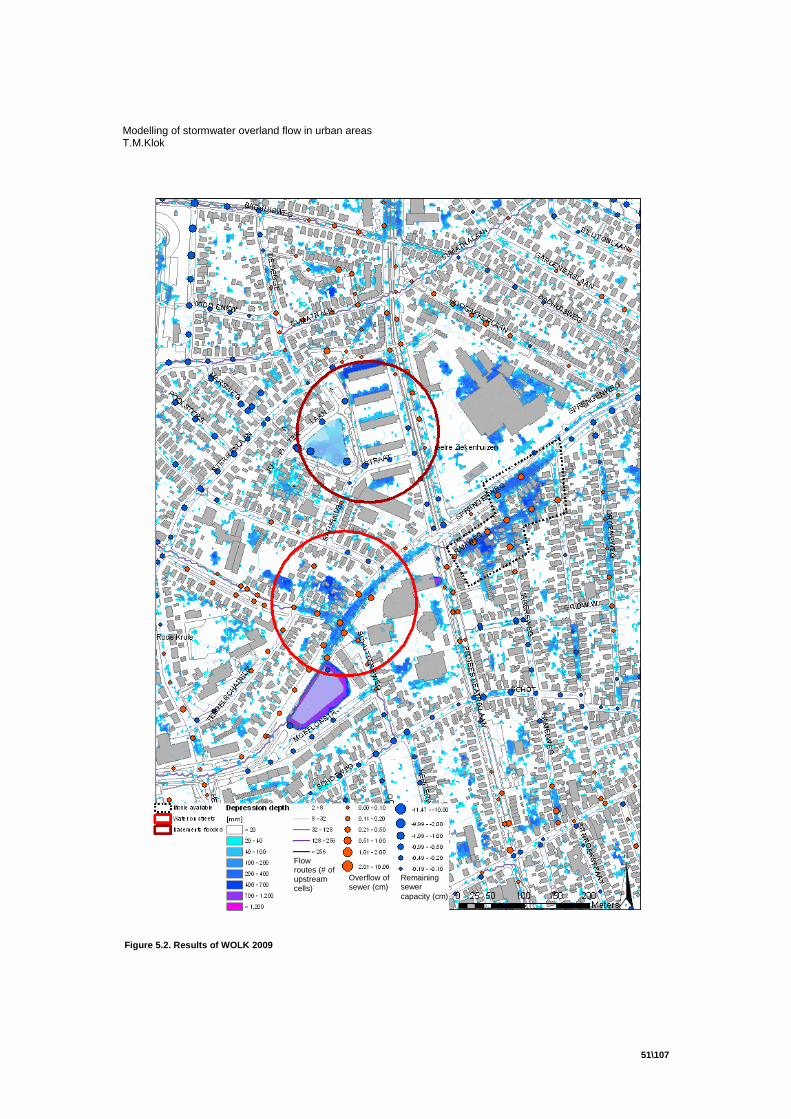
Modelling of stormwater overland flow in urban areas T.M.Klok
51\107
Figure 5.2. Results of WOLK 2009
Remaining sewer
capacity (cm)
Overflow of sewer (cm)
Flow routes (# of upstream cells)

Modelling of stormwater overland flow in urban areas T.M.Klok
52\107
Figure 5.3. Results of WOLK 2011
Flow routes (# of upstream
cells) Overflow of
sewer (cm)
Remaining sewer
capacity (cm)

Modelling of stormwater overland flow in urban areas T.M.Klok
53\107
5.3 SWOT analysis Based on the above assessment of WOLK, as well as the assessments in previous chapters the strengths and weaknesses of WOLK can be summarized in a SWOT-analysis. Table 5.2. SWOT-analysis of WOLK 2011
Strengths Few input parameters Visual output with maps Possibility to combine with output from other
models
Weaknesses Overestimation of overland flow WOLK cannot handle large data files Overland flow routing is limited to 1-directional
flow Can only simulate ”end situation” and routings Run time
Opportunities Increase in precipitation intensity demands
more overland flow modelling WOLK can also be used for other purposes
Threats Municipal budget for runoff models in relation
to cost of model Municipalities tend to rely more on expert
knowledge Other, similar, overland flow models
Strengths The strengths of WOLK are that the number of parameters required to run WOLK is small. Only a DEM, impermeable surface and a precipitation amount are required. The output of WOLK is also a strength, because the GIS environment allows for a wide range of views, including the possibility to combine WOLK results with results from other models, such as Infoworks CS. Weaknesses The weakness of WOLK that it cannot handle large amounts of data, is the cause for a large preparation time of the data which is used as input for WOLK. For instance, large DEMs have to be cut into smaller sections. The borders of these sections have to be chosen well, because otherwise the results of the model are influenced. Well chosen borders are for instance located in open water or high grounds, such as railways. These borders are essentially natural catchment boundaries. The overland flow is also a weakness of WOLK, because the output it generates is unusable for the development of measures. The same goes for the time dependency of WOLK. The output of WOLK only shows an “end situation”, but it is unknown when this situation is reached. Furthermore it is expected that when time is incorporated in WOLK the results will be different, but this assumption has to be proven in further research. An alternative model should be build, which is time based and which allows for a spreading of water flows to several adjacent cells. Opportunities Opportunities for WOLK are the expected increase of precipitation intensity by the KNMI. An increase in precipitation will increase the amount of overland flow. The need for models which can predict overland flow is likely to increase in the future. Next to that, WOLK can also be used for other purposes, such as the estimation of contaminated flows caused by industrial fires or other failures. Incidents like with the Chemie-Pack fire at Moerdijk in the Netherlands showed that possibility. Threads A thread to WOLK is the municipal budget for such models, because at the moment the largest client group is municipalities. One way to deal with this thread is to shift the use of WOLK more to fire fighting water flows, instead of precipitation flows. Although more research should be done to model the processes related to fire fighting water flows. The client group for such model analysis

Modelling of stormwater overland flow in urban areas T.M.Klok
54\107
would be commercial, like industry, instead of the governmental client group for a regular WOLK. It is unknown at the moment if there is a valid market for fire fighting flows. The first scouting projects were not finished at the time of this research. The next thread to WOLK are the municipal experts, because they mostly have to work with the WOLK output. If these people trust their own experience more, and do not see the value of WOLK, WOLK might become unused. On the other hand should experts not blindly trust the WOLK output, but they have to trust their own experience too. The last thread is considered to be similar overland flow models from competitors. One example is Wodan from Grontmij, because this model works slightly different it can have a market advantage.Keep developing WOLK should keep it up to date and help being competitive with similar overland flow models.
5.4 Conclusion The assessment of WOLK for the city of Apeldoorn with both AHN-1 and AHN-2 elevation models has shown several similarities as well as differences. As expected, most issues regarding the model results of WOLK remain with a newer version of the DEM. The assessment shows that the principle of WOLK itself is acceptable, in the sense that the simulated locations of inundation are similar to the experienced inundation, although when the WOLK results are compared to reality the sizes and depths of the depressions are overestimated up to two decimetres, although mostly less. If a verdict has to be made whether or not the use of AHN-2 improves the results of WOLK, then the verdict would be to use it. Mainly because the data is more up to date, furthermore the AHN-2 data does not have to be filtered anymore. Another advantage of AHN-2 is the amount of sample points per square meter which has increased compared to AHN-1. The methodology of WOLK itself is also subject of debate. The assumptions which lie at the base of WOLK should be reconsidered, because these assumptions cause the overestimation of overland flow. An increase of the infiltration/sewer parameter for instance should result in more accurate output. Two other possible solutions to the overestimation of the depression sizes is to use a dynamic flow model, instead of a catchment based single directional flow model. Runoff might flow differently when a rainfall event can be simulated over a period of time. This conclusion is also in line with the SWOT analysis, which has been performed in order to get an overall view of the various strong points and challenges concerning WOLK. The SWOT analysis summarizes the most prominent aspects of WOLK. The conclusion based on both the assessment of WOLK 2009, 2011 and the SWOT analysis is that the WOLK methodology has shortcomings. The user guide will help to minimize inconsistencies in working method, but other limitations, such as flow routing, intermediate results and time dependency remain. It is therefore worth investigating whether alternative model structure could solve the shortcomings of WOLK.

New model
6
An alternative overland flow model


Modelling of stormwater overland flow in urban areas T.M.Klok
57\107
6 New model
The previous chapter discussed the need for an alternative overland flow model. The main reasons for a different overland flow model are the unknown time scale in WOLK, thus only the final results of the computations are shown. Furthermore, the flow possibilities in WOLK are limited to only one direction. A requirement from the municipalities is also that the runtime of a model should be as low as possible, while still producing accurate results. With these three main requirements in mind a new overland flow model has been developed. The idea was to stay close to the assumptions made in simplified overland flow models (chapter 2), because the results from these models have proven to be relatively in line with practise. Thus, the assumptions that are used for the new model similar to those of WOLK:
- Precipitation will only flow from impermeable surfaces such as buildings and paved areas.
- A precipitation event of 60 mm in one hour will be taken for simulations, where 20 mm will infiltrate, evaporate or runoff into the sewer system. Therefore only 40 mm will become overland flow.
- The overland flow will be simulated based on Manning‟s flow equations. - The DEM will be unchanged, so a regular square spaced grid will be used. All other
layers will use the same type of raster. - Flow direction will be evaluated per grid cell. - Locations of impermeable areas, buildings and open water are the same as in the WOLK
2011 case. Model input For the development of the new model several input data are available, which is shown in figure 6.1. The surface elevation in the form of a DEM is based on the AHN data. The DEM remains the most important input data source, because the DEM has a significant influence on the results of the model. On top of the DEM the locations of impermeable surfaces are laid out. As described in the assumptions, the impermeable surfaces determine where rainfall will turn into overland flow. The impermeable areas can also be used in the determination of a roughness coefficient, which is needed when the model becomes time depended (Bates & De Roo, 2000; Berthier et al., 2004). The roughness coefficient would then become a forth layer. The top most layer in figure 6.1
shows at which locations open water is available. Furthermore this layer can be used to specify the locations at which precipitation will be located, for instance when rainfall occurs on a small portion of a larger case area or to simulate regional variability in rainfall intensity. Combining the three data sets in such a way that the overland flow is accurately simulated is the goal of this research section.
Figure 6.1. Available input for alternative models
Paved area & buildings
Surface elevation
Water
Roughness coefficients
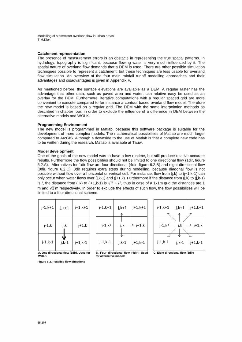
Modelling of stormwater overland flow in urban areas T.M.Klok
58\107
Catchment representation The presence of measurement errors is an obstacle in representing the true spatial patterns. In hydrology, topography is significant, because flowing water is very much influenced by it. The spatial nature of overland flow demands that a DEM is used. There are other possible simulation techniques possible to represent a catchment, but these techniques are less usable for overland flow simulation. An overview of the four main rainfall runoff modelling approaches and their advantages and disadvantages is given in Appendix F. As mentioned before, the surface elevations are available as a DEM. A regular raster has the advantage that other data, such as paved area and water, can relative easy be used as an overlay for the DEM. Furthermore, iterative computations with a regular spaced grid are more convenient to execute compared to for instance a contour based overland flow model. Therefore the new model is based on a regular grid. The DEM with the same interpolation methods as described in chapter four, in order to exclude the influence of a difference in DEM between the alternative models and WOLK. Programming Environment The new model is programmed in Matlab, because this software package is suitable for the development of more complex models. The mathematical possibilities of Matlab are much larger compared to ArcGIS. Although a downside to the use of Matlab is that a complete new code has to be written during the research. Matlab is available at Tauw. Model development One of the goals of the new model was to have a low runtime, but still produce relative accurate results. Furthermore the flow possibilities should not be limited to one directional flow (1dir, figure 6.2.A). Alternatives for 1dir flow are four directional (4dir, figure 6.2.B) and eight directional flow (8dir, figure 6.2.C). 8dir requires extra steps during modelling, because diagonal flow is not possible without flow over a horizontal or vertical cell. For instance, flow from (j,k) to (j+1,k-1) can only occur when water flows over (j,k-1) and (j+1,k). Furthermore if the distance from (j,k) to (j,k-1)
is , the distance from (j,k) to (j+1,k-1) is , thus in case of a 1x1m grid the distances are 1
m and m respectively. In order to exclude the effects of such flow, the flow possibilities will be limited to a four directional scheme.
A. One directional flow (1dir). Used for WOLK
B. Four directional flow (4dir). Used for alternative models
C. Eight directional flow (8dir)
Figure 6.2. Possible flow directions
j,k
j,k+1 j+1,k+1
j+1,k
j+1,k-1j,k-1j-1,k-1
j-1,k
j-1,k+1
j,k
j,k+1 j+1,k+1
j+1,k
j+1,k-1j,k-1j-1,k-1
j-1,k
j-1,k+1
j,k
j,k+1 j+1,k+1
j+1,k
j+1,k-1j,k-1j-1,k-1
j-1,k
j-1,k+1

Modelling of stormwater overland flow in urban areas T.M.Klok
59\107
6.1 Computation methodology of new model The different versions are based on different concepts for the simulation of overland flow. The concepts range from intuitive to theoretical based overland flow computation methodology. All versions have in common that they are based on the same principles: same input data and same build up of layers is used. Below the two main concepts will be discussed. 6.1.1 Intuitive distribution model The first version of the new model uses a method where all water from the origin cell (j,k) is taken and divided over all possible lower adjacent cells (equation 6.1). The goal of this alternative model is to use a 4-directional flow routing scheme and compute the results within minimal amount of runtime. This method is not time depended. In order to determine in which direction(s) the water will flow the DEM is used as well as the water layer. The real elevation and water level layers are summed up and form a total elevation layer (figure 6.7). The relative elevation difference from origin cell (j,k) to each adjacent cell is computed (equation 6.6). If a destination cell has a higher total elevation, then no water from the origin cell will reach it. This method only computes water flowing downhill, thus cells with a higher elevation are neglected. On the other hand, if a destination cell has a lower total elevation, then water from the origin cell is able to flow to the that destination cell, see also figure 6.3. The amount of overland flow that each of the lower destination cells receives is based on the elevation difference between two destination cells (equation 6.10).The equation shows only the flux into one of the four directions.
(6.1)
Where: = the flux between the origin cell (j,k) to a destination cell (j,k+1).
= the available precipitation volume in the origin cell
= the slope between the origin cell (j,k) to a destination cell
An example of the use of the model: two destination cells with the same total elevation will receive both 50% of the water from the origin cell. Whereas if one cell would have been twice as low as the other, the division would be 33% and 66%. At the end of the computation the origin cell is always empty. This computation cycle is repeated for each grid cell in the case area, which completes a single iteration. By re-evaluating the whole grid several times, in the order of 25,000 iterations, the final distribution of overland flow is computed.
t = t0
t = t1
Figure 6.3. Division of overland flow in an intuitive form

Modelling of stormwater overland flow in urban areas T.M.Klok
60\107
The main concerns with the empirical method are the lack of knowledge about the flow through time. Therefore a new version has been developed in which the flow of water has a time factor included in the computations. 6.1.2 Manning-based model
The Manning based overland flow model is based on the principles used in the LISFLOOD-FP model, as described by Bates & de Roo (2000) and Hunter et al. (2005). The LISFLOOD-FP model is originally used to simulate the wetting and drying of floodplains. This process is similar to the wetting and drying of surfaces in an urban area due to extreme rainfall events. An advantage of this script is that it also works with a 4-directional flow scheme. Although a disadvantage is that the time step has to be kept minimal in order to keep the model stable. The Manning based model is based on the St Venant equations, for which a description can be found in Appendix C. Two-dimensional overland flow is most often a slow and shallow phenomenon, with the exception of flood situations like dam-breaking. As such Bates & de Roo (2000) and others assume that overland flows are primarily influenced by bed roughness rather than velocity coefficients based on surface elevation differences, thus allowing for the inertial term to be neglected from the St Venant equations. A disadvantage of this method is that any supercritical effects are thus excluded. Each cell in the model is seen as a storage cell. The advantage of a storage cell method is that the fluxes are calculated analytically so the computational cots per time step are potentially lower than in equivalent numerical solutions of the full shallow water equations. t = t0
t = t1
Figure 6.4. Division of overland flow in a Manning-based form
The flow from an origin cell to its adjacent four neighbour destination cells is determined by the Manning formula (equation 6.3). The amount of overland flow that a destination cells receives depends on waterlevel differences, the roughness and the time step (see also figure 6.4). The flux out of the origin cell has to be limited, in order to prevent that more water leaves a cell than is available (figure 6.5). When the time step is chosen small enough, the model will be stable. The numerical scheme of the Manning based overland flow model will be discussed in the next section.
Figure 6.5. Limiting procedure
Original situation
End situation if no limiting is
used
Limiting procedure
End situation if limiting is used

Modelling of stormwater overland flow in urban areas T.M.Klok
61\107
6.2 Numerical scheme Both new models are based on the same numerical scheme, with the exception of the discharge determination. Due to the complexity of the Manning based model, the numerical scheme for this model will be described in this section. The numerical scheme of the Manning based model has been developed with a minimum amount of processes steps required. Most of the information about flow routing is derived from the DEM. The simplest way to model distributed routing of water is by treating each raster cell as a storage volume for which a continuity equation has to be solved (Bates & De Roo, 2000). The change in precipitation volume over time is therefore equal to the fluxes into and out of each cell during a time step.
Figure 6.6. Definition of positive directions in theoretical model
(6.2)
Where: = the precipitation volume per cell [m
3]
= time [s]
= discharge flow rates into or outside the reference cell. [m3 s
-1]
The equation above is solved explicitly using a finite difference discretization of the time derivative term. Therefore:
(6.3)
The volume can be rewritten as its individual parameters:
(6.4)
Where, and are the cell sizes in [m]. If , then can be written as: .
Combining equations 6.2, 6.3 and 6.4 gives:
(6.5)
Discharge is normally formulated as: (6.6)
Qj+1,kV
Qj,k-1
Qj,k+1
Qj-1,k
+

Modelling of stormwater overland flow in urban areas T.M.Klok
62\107
The velocity rates are computed using the Manning equation, although other flow formulas, such as Chézy, can also be used (Klok, 2011). The velocity is computed in four directions relative to the origin (j,k) cell. Equation 6.7 and further only describes the computations for one direction (j,k) -> (j,k+1). The flow velocity between two adjacent cells is then described as:
(6.7)
Where: = flow velocity between the cells (j,k) and (j,k+1). [m s
-1]
= the hydraulic radius at the interface of the cells (j,k) and (j,k+1). Normally the waterlevel [m]. = the water surface slope between the cells (j,k) and (j,k+1).
= the Manning friction coefficient. [m1/3
s-1
]
The hydraulic radius is normally defined as . But it can also be written in terms of :
(6.8)
Where: = the cross-sectional area in the interface between the cells (j,k) and (j,k+1). [m
2]
= wetted perimeter [m]. Is constant 1 meter in case of a 1x1 meter grid.
For an overview of parameters, see also figure 6.7 Combining equation 6.5, 6.7 and 6.8 gives the amount of discharge per time step between two cells. and are written in terms of . The flux between two adjacent cells in the direction is
then described as:
(6.9)
Where: = the discharge rate between the cells (j,k) and (j,k+1). [m
3 s
-1]
= the cross-sectional area in the interface between the cells (j,k) and (j,k+1). [m2]
Figure 6.7. Overview of the parameters used

Modelling of stormwater overland flow in urban areas T.M.Klok
63\107
Some remarks concerning the parameters in equation 6.9, for simplicity the Manning friction coefficient will only be varied for two types of surfaces: paved and unpaved areas. The values for these types of surfaces have been taken from the Manning table from Chow (1959). For paved (semi-impermeable) surfaces an average is taken from the road types: asphalt, concrete and stone pavement. The average gives a Manning friction coefficient of 0.015 m
1/3 s
-1. The coefficient
for unpaved area is an average of the surface types: grassland, crops and forest. The average gives a Manning friction coefficient of 0.030 m
1/3 s
-1. This assumption is considered sufficient
given all other uncertainties. The water surface slope is computed as:
(6.10)
Where: = surface elevation + water level in the cells (j,k) and (j,k+1). [m]
= length between the cell centre of the cells (j,k) and (j,k+1). [m] When the slope is negative, thus , the flux in that direction will be neglected. The
model works with a 1x1m grid, therefore:
(6.11)
Equations 6.9 and 6.11 can be combined and rewritten as:
(6.12)
In order to prevent more water leaving a cell than it contains, a limiter is introduced. To achieve the right amount of discharge from a cell, the discharge rates , , and are
first calculated as described above and then limited by a non-dimensional coefficient .
(6.13)
Where: = limiter coefficient [-]
= volume of water in the cell at time . [m3]
= discharge flow rates into or outside the reference cell. [m3 s
-1]
= time step. [s]
The limiter is only used during the drying up phase of a cell, thus when:
(6.14)
If a limiter is used, the limited flux is computed as .
Combining equations 6.5, 6.12 and 6.13 and 6.14 and solving them for each raster cell produces the results for one time step. Thus by evaluating the complete raster several times, the overland flow is simulated.
Modelling of stormwater overland flow in urban areas T.M.Klok
64\107
6.3 Testing Both the intuitive distribution model and the Manning-based model have been tested in order to assess their performance. The models have been assessed based on the cases shown in figure 6.8. These cases have been selected, because they can also occur in normal urban overland flow simulations. The models should be able to handle relative small volumes of water and large elevation differences between two cells. The small black lines in the figures show where overland flow is expected. The DEM is coloured from red to green, with red high elevation and green low elevation. The building in the centre of the map is an obstacle for the flow of the water. The depression in test 1 and 2 marks the expected location where the overland flow will be gathering. The dimensions of each test area are 21 by 21 cells, on a 1x1m grid. Thus the test area is 21 by 21 square meters. The amount of precipitation that is used is the same as in the overland flow cases, namely 40 mm. All values are calculated in meters. The lowest point has an elevation of -2 meters, while the highest point has an elevation of 10 meters. The negative elevation is chosen, because normal DEM elevations are computed relative to the Dutch Ordnance level (NAP), thus negative elevations can occur. The building and blockade have an elevation of 20 meters. During test 1 (figure 6.8a) the overland flow is expected to split and flow on both sides around the building. The amount of flow on each side should be equal. After the building the flow should recombine and flow towards the lowest point, the depression. In test 2 (figure 6.8b) the precipitation is located on top of a small, high surface. In this case a building. Due to the 4-directional flow scheme, the runoff should flow of the building on four sides. Then it should flow towards the lowest point on the left down corner. Unlike test 1 and 2, test 3 (figure 6.8c) uses a flat surface. The precipitation source is located on the centre cell, without extra elevation. The expected results are that the precipitation should disperse over the complete area via a regular pattern. Furthermore should the flows to each side be equal. Test 4 (figure 6.8d) again uses a sloped surface, but this time a slope from right to left. In the middle of the surface a blockade is formed. Water can only pass the blockade via a small gap in the centre. Water is released on one side of a blockade. The water is expected to flow through the blockade and disperse on the other side. Finally all water should have flown to the left side and collect at the lowest points.

Modelling of stormwater overland flow in urban areas T.M.Klok
65\107
Figure 6.8. Test situations for the new models.
6.3.1 Results Manning-based model The results of the tests show that the Manning-based model is relative slow, compared to the intuitive distribution model. The Manning-based model performs as expected. The flow behaves as predicted before. What can be seen from the Manning-based model is that the front of a water body flows relative rapidly, while the drying up and the back goes relative slow. Again, this is in line with what is expected from practise. Figure 6.9.A to D show some results during the computations of the various tests, which prove that the tests perform as expected. More extensive results can be found in Appendix H. The goal of the Manning-based l model was to simulate overland flow in a way that the time scale was known, the flow directions were according to a 4-dir or 8-dir scheme, and preferably that the results can be used in a quantitative assessment of a flood area. Both these goals have been met. The Manning-based model has been tested with several time steps. A smaller time step ensured a more smooth flow of the water. The maximum time step which could be used during the testing was 2 seconds, although best results were produced with time steps between 1 and 0.1 second. Time steps smaller than 0,1 second resulted in model run times which are practically unusable for large research areas. Another test for the Manning-based model was to investigate the influence of the limiting procedure. When no limiter is used, the fluxes became larger than the total volume of water available, which resulted in negative water volumes. With the limiter enabled, this behaviour did not occur. The volume of water in a cell returned to zero smoothly.
Building
Water
Depression
Water + building
Depression
Water
a. Test 1: flow around object b. Test 2: flow originating from high point
c. Test 3: flow dispersion on flat surface
Wa
ter
d. Test 4: flow through small opening in blockade
blo
cka
de
blo
ckad
e

Modelling of stormwater overland flow in urban areas T.M.Klok
66\107
A. Theoretical model during test 1
B. Theoretical model during test 2
C. Theoretical model during test 3
D. Theoretical model during test 4 Figure 6.9. Selection of test results of Manning-based model. More extensive results can be found in Appenidx H.
Intuitive distribution model The tests also have been executed for the intuitive distribution model. The general results of the intuitive distribution model are in line with the results from the Manning-based model. The amount of iterations required to produce the results was about 10% of the amount of iterations from the Manning-based model, which was one of the goals of the intuitive distribution model. But the way in which the results are produced give reason for debate. The results are influenced by the way in which the raster is processed. Furthermore a „checkerboard‟ effect can occur, which has been described by Hunter et al. (2005). The effect causes the overland flow to rapidly change positions over and over. The intuitive distribution model can be used to get an idea how the overland flow will develop over time, which time scale is unknown, but the results cannot be used in a quantitative analysis. WOLK-AML WOLK has not been executed for the test cases, but the model will show only the final result, thus the overland flow which has gathered in the lowest point in test 1, 2 and 4, while in test 3 the water will be evenly dispersed over the complete basin, except for the building. The flow lines will show that the overland flow will flow only on one side of the building in test 1 and 2. In test 3, flow lines will be seen diverging from the building. The flow lines in test 4 will show that the overland flow choose a single straight path to the lowest point in the basin, rather than the behaviour seen in 6.9.D.
6.4 Conclusions The current overland flow models have some drawbacks, such as the time scale, the flow scheme (1-directional) and the runtime. Furthermore it would be an advantage if the results of the current
Modelling of stormwater overland flow in urban areas T.M.Klok
67\107
overland flow model could be used in a quantitative analysis. The models developed in this chapter had to meet these goals. Therefore two alternative models have been developed, an intuitive distribution model and a Manning-based model. The intuitive distribution model does not give any information about time scale. The only advantages of this model were a low runtime of 10% of the intuitive distribution model and the 4-directional flow routing possibilities. It is unknown if the runtime of the intuitive distribution model is lower compared to that WOLK. Therefore a comparison between the intuitive distribution model and WOLK should be performed. In the Manning-based model on the other hand the flow is time depended in a 4-directional routing scheme. This resulted in a larger runtime of the Manning-based model compared to the intuitive distribution model. In order to assess the differences between the intuitive distribution model and the Manning-based model some test cases have been set up. The results from the tests show that the intuitive distribution model performs not as expected. The flow in general is acceptable, in the sense that water does flow downhill, and the results are produced faster than the Manning-based model, but that is all. On a small scale, like the test cases, the model is not usable due to the checkerboard effect. It is expected that this effect is less significant on larger scale case areas, due to the topography of an urban area. There is less interaction between the water containing cells, and overland flow has more directions to flow to. The Manning-based model on the other hand gave results which were in line with the expected physical behaviour. The time step which had to be used was small, resulting in a large runtime of the Manning-based model. Furthermore, the time reference scale is an advantage compared to the intuitive distribution model. The results could be used in a quantitative analysis. Therefore all goals have been accomplished with the Manning-based model, except for the runtime. The intuitive distribution and the Manning-based model both have the potential to give reasonable results. Therefore both models will be assessed and compared with WOLK results and with results from practise. Testing both versions of the new models against cases which also have been modelled with WOLK, should prove whether the new models produce results which are in line with WOLK results and if the new models are usable in practise or not. After that it can be concluded if WOLK can be improved with the alternative models.


Comparison of WOLK and alternative models
7


Modelling of stormwater overland flow in urban areas T.M.Klok
71\107
7 Comparison of WOLK and alternative models
The performance of the newly developed models has been assessed with test cases, but the real test will be the assessment of the intuitive distribution model and the Manning-based model against the results from WOLK. In order to do so, three areas have been selected. For all three areas a WOLK has recently been executed. The case areas are the village of Uddel, Deventer centre and a fire fighting water case. The research case from chapter 5 could not be used for this assessment, because the case area is too large, which resulted in unwanted large runtimes for both the alternative models.
7.1 Cases The first area is a typical WOLK case of an urbanized area. The case area is the village of Uddel, which is part of the municipality of Apeldoorn. The DEM is based on AHN-2 data. The village is surrounded by woods and agricultural land. Therefore it is assumed that only a minimal amount of overland flow is entering the system from the sides. Furthermore, the precipitation in both new models enters the system the same way as WOLK: via the impermeable surfaces. The second area is different in the sense that it has been used for a WOLK fire fighting water flow case. The computation methodology is the same as for normal WOLK computations. The main difference is the amount of water and the starting locations of the water. The possibilities for a fire fighting modelling case have been discussed in the SWOT analysis in chapter five. The amount of water that is available in a fire fighting case is based on data from industrial fire fighting cases,
such as the recent fire at Chemie-Pack, Moerdijk in the Netherlands. The total amount of water that has been used there during the fire extinguishing is about 2.5 m
3 per square meter of burning
building. The fire took ten hours before it was put out by fire fighters. The resulting flow from the factory site contains all kinds of pollutions. From environmental and health perspective it is important to know where the contaminated waste water will flow to. In this way measures can be taken to prevent polluted water to flow to unwanted locations such as agricultural land or urbanized areas.
The third case is the city centre of Deventer. The Deventer case is used for the comparison, because for this case detailed complaints are available. The DEM is based on the older AHN-1 data. These data are less accurate, which will influence the results of all models. The comparison will be limited to the intuitive distribution model, not the Manning-based model. Due to the area size of almost 2 million square meters, the runtime of the Manning-based model would be too large. Deventer centre is almost completely surrounded by water. Therefore the area is assumed to have no interaction with surrounding areas.
Figure 7.1. Fire at Chemie Pack, Moerdijk, the Netherlands (Zantingh, 2011)
Modelling of stormwater overland flow in urban areas T.M.Klok
72\107
7.2 Comparison of results 7.2.1 General The goals for the new models have been formulated in chapter five and they were: low runtime, improved flow scheme, temporal flow characteristics and time depended computations. The comparison of results from WOLK and the intuitive distribution model and Manning-based model is based on these goals. The results for the two test cases are presented on the next pages in figure 7.2 through 7.4. Runtime From this analysis can be concluded that both the intuitive distribution and the Manning-based new model are not suitable for large research areas. The runtime per iteration just take too long, because each cell has to be evaluated individually, which makes it economical irresponsible. An iteration consists of the evaluation of the complete case area. The use of the new model will therefore only be reviewed for small research areas (<250,000 cells). Therefore the runtime goal for the new models is met partially, because the runtime is only minimal for small research areas. The runtime of the new models was in line with the expectations from the test runs. The intuitive distribution model was able to compute the overland flow faster compared to the Manning-based model. An issue that came up with especially the intuitive distribution model is that it is unknown when the model is finished with computing, because there is no stopping rule. A stopping is difficult to implement, because of the checkerboard effect (Hunter et al., 2005). This effect prevents the overland flow to stop flowing completely. The Manning-based model does not have this problem, because one can set a desired simulation period, ranging from one second up to several hours, although the latter is unreliable, because the Manning-based model is still too simplified to model over a period longer than several hours. This is because some neglected runoff processes become relevant when simulated over a longer period. For instance the evaporation and groundwater change: the infiltration can no longer be seen as a constant parameter. Furthermore, is it likely that new rainfall events occur when even longer periods are modelled, thus influencing the simulating outcome. Time dependent flow routing Furthermore the model has the possibility to show results during the computations. During the calculation both the intuitive distribution model and the Manning-based model create a time lapsed gif. When the gif is opened the results appear as flowing runoff. The time lapsed gif proved to be helpful in the overland flow assessments. The gif made clear where certain amounts of water had flown, compared to static results with runoff routes. Other shortcomings of WOLK are the flow possibilities and the information that can be derived from the analysis, see also chapter 5. The model shows only the final results, when all the water is either flown out of the system, or caught in depressions. The streamlines represent where the water has flown, although these streamlines are based on the assumption that all the water will always flow in the steepest downhill direction. The alternative models do not have these specific disadvantages. The flow of water is simulated by computing for each individual cell the amount of water and the direction in which it will flow. Water is able to flow in 4 directions (4dir), based on water level differences between the four adjacent cells. Due to the 4 directional flow scheme, results of the new models are different compared to the results of the one-directional flow in WOLK, although the similarities between the two models are stunning.

Modelling of stormwater overland flow in urban areas T.M.Klok
73\107
7.2.2 Uddel The results from Uddel (figure 7.2) are compared with complaints registered by the municipality of Apeldoorn. The precipitation amount in both cases is 60 mm where on impermeable surfaces 40 mm becomes overland flow. The locations of impermeable surface are based on data from 2011. The DEM in both cases is based on AHN-2. The complaints show that in general there are no large overland flow related flood problems. The only real issues are at the location marked with a number 3 in figure 7.2.A. The crossing at that location is known to flood during extreme rainfall events. Both WOLK and the new models do not simulate this correctly. The cause for this lies in the subsurface: the sewer system. At that specific location the sewer will overflow, according to Infoworks simulations. Overland flow models will not be able to simulate this behaviour correctly, unless they also compute the sewer system. Locations 1, 2 and 4-6 in figure 7.2 mark locations where there is a difference between the intuitive distribution model and the WOLK-AML. At location 1, the new model shows a flooded road, while in the AML results there is no flood. The difference is likely to be caused by the way in which the new model works: it takes a relative large amount of time before this street is cleared from overland flow. The new model should have been executed for a longer period of time. The number of iterations should be increased in order to compute the overland flow leaving location 1. The numbers 2 and 4 mark locations where the depression area is larger in the new model results compared to the WOLK-AML results, while number 5 and 6 are locations where the AML computes a larger depression compared to the new empirical model. The only explanation for these differences can be found in the 4 directional flow scheme from the new models, as well as the more realistic flow depth. At this moment it is unknown if and which model is correct.

Modelling of stormwater overland flow in urban areas T.M.Klok
74\107
A). Results of WOLK.
B). Results of the intuitive distribution model.
Figure 7.2. Map of Uddel (municipality of Apeldoorn). Green-red represents low-high surface elevation; depressions are shown in blue; impermeable surfaces (buildings and roads) are shown in gray.
1
2
3
4
5 6

Modelling of stormwater overland flow in urban areas T.M.Klok
75\107
7.2.3 Fire fighting water The second case which has been used to compare WOLK and alternative models is a fire fighting case. In both models the same DEM and impermeable surfaces are used. The DEM is based on AHN-2 data. The results of both types of models differ significantly. The difference is mainly caused by the flow procedures in both types of models. This difference manifests itself at locations of open water. The WOLK-AML works with catchments and open water is modelled as a single catchment, therefore when overland flow reaches open water, it will immediately disperse over a large area. The new models on the other hand treat open water just as any other surface. Overland flow which reaches open water will disperse each time step with a certain amount, with a maximum of the current cell value of a grid cell. Therefore by default it would take several time steps until the effect of the overland flow is measurable over the complete section of open water. The computation method of the new models causes an unwanted build up of water at the entrance location of the open water. In case of small sections of open water, as is the case at locations 1 and 2 in figure 7.3, the overland flow reaches the opposite site of the open water and continues flowing on land. This effect is unrealistic, and therefore unwanted. A solution for the open water effect is to treat open water as a single cell or a single catchment, thus replicating the effect as described in WOLK-AML. Another possibility is to treat open water as nodata, thus eliminating the open water from the simulation. Overland flow will only be able to enter open water, but it will not be able to leave it. In case of a pool or a small gutter, this method will not produce realistic results, because a pool or gutter should be able to overflow. Therefore the transformation of open water to nodata should be executed with care. Another effect which causes unrealistic results in the new models is the initial set-up of the models. The fire fighting water is simulated as water which at t=t0 located adjacent to the relevant buildings, the orange buildings in figure 7.3. This results in unrealistic high water values of several cubic meters at these cells. More realistic results would be obtained when the fire fighting water is entering the computational area over a certain period, for instance one hour. Each time step a certain amount of water should be added to the model, instead of the complete amount at the beginning of the simulation. This large amount acts like a flash flood in the model, instead of overland flow. Only the Manning-based model is suited for such inflow spread over time, because both the WOLK-AML and the intuitive distribution model have an unknown time scale. From the comparison of WOLK and the intuitive distribution model in fire fighting cases can be concluded that the set-up of the DEM has a significant influence on the results of all models. The issue with the fire fighting cases is that there are no data to check the model results with. Only after an event data can be acquired. Therefore it is unknown at the moment if and which model is correct.

Modelling of stormwater overland flow in urban areas T.M.Klok
76\107
A. Results when the original WOLK-AML is used.
B. Results when the intuitive distribution model is used.
Figure 7.3. Results for the inundation and overland flow due to fire fighting water.
1
2
Modelling of stormwater overland flow in urban areas T.M.Klok
77\107
7.2.4 Deventer Centre The third case for comparison is the city centre of Deventer. Again, the results of the intuitive distribution model are similar to the results of WOLK-AML. Some depressions in the intuitive distribution model are larger compared to the WOLK-AML. The depression at location 1 in figure 7.4.A is larger compared to the same location in figure 7.4.B. According to complaints registered by the municipality, the depression at location 1 has never been reported. Therefore both models are inaccurate. A possible explanation for the inaccuracy is that the DEM is likely inaccurate, which is caused by the use of AHN-1 data. AHN-2 allows for a smaller cell size, thus increasing the accuracy of the DEM. Furthermore, it is likely that an alley is missed in the surface data, which is caused by the impermeable surface data. The source for this data is a Top10 vector. The depression at location 2 in figure 7.4.B is significantly larger compared to the depression in figure 7.4.A. The only explanation for this result is that the intuitive distribution model required more iterations before an end situation was achieved. Figure 7.4.B. therefore shows a snap shot of results during computations. Running the intuitive distribution model for a longer period of time would allow the runoff to reach the open water and flow into it. The location of this water nuisance is also reported by inhabitants for the area. Therefore it is assumed that the location of the depression is correct, although the size, as modelled by the intuitive distribution model, is too large. The third location as marked in figure 7.4.B. shows another difference between the WOLK-AML and the intuitive distribution model. The area is a park with mostly grassland and scattered trees. The overland flow is generated from the park roads. In practice, such areas have several smaller depressions, due to the nature of grassland. Therefore the intuitive distribution model could have modelled the overland flow correctly. Another explanation can be that the model has to run for a longer period of time, thus allowing the overland flow to reach open water, which is next to the park. From the comparison of both models in the Deventer case can be concluded that it is important to know when the new model has reached an end state in which all overland flow has either reached a depression or has left the system. Therefore an improvement for the intuitive distribution model would be to enclose some sort of stopping rule for the model. As stated before, this is difficult to implement, because of the checkerboard effect.

Modelling of stormwater overland flow in urban areas T.M.Klok
78\107
A. Results when the original WOLK-AML is used.
B. Results when when intuitive distribution model model is used. Figure 7.4. Results for Deventer Centre for WOLK and the intuitive distribution model. Dark blue are inundation areas, light blue is open water, grey is buildings and white is grassland.
1
2
3

Modelling of stormwater overland flow in urban areas T.M.Klok
79\107
7.3 Conclusion The goals for the new models were: low runtime, improved flow scheme, temporal flow characteristics and the presentation of results. Based on the goals formulated for the new models and the comparison of the new models with WOLK-AML can be concluded that the goals are met partially. The first goal, not only showing final results, has been achieved. Both new models have the possibility to create time lapsed gifs as well as GIS maps of intermediate results. These intermediate results are partly the reason why the new models have a larger runtime compared to WOLK-AML. The second goal, the low runtime, has not been met. The runtime of the new models, especially the theoretical model, is in most cases much longer compared to the WOLK-AML. The third goal was the improved flow scheme. Both new models apply a four-directional flow scheme, although with differences. The 4-directional flow scheme results in different simulations compared to a one-directional flow scheme. It depends on the scale at which the results are reviewed. On macro scale, the results of both types of flow schemes do not vary significantly, although on micro scale they can do. A micro scale assessment of the results is for instance an assessment to determine the water level against houses, for instance for flood damage estimations. In that case the Manning-based model could be applied. When only general flow patterns are required, both the intuitive distribution model and WOLK can be used. The WOLK-AML can be applied when only the final state of the overland flow is relevant. The flow paths in the WOLK-AML are for reference, because they give less information than the flows in the new models. A disadvantage of the new models is that there is no record of the flow paths, therefore at the end of the analysis it is unknown how much water has discharged through a particular street for instance. The models should have to be adapted for this analysis. The fourth goal concerns the time dependency in the overland flow computations. The flow of runoff should be related to a time scale. Such an improvement can give more information about the durations of floods. The Manning-based model has reached this goal. The model is able to compute overland flows based on Manning‟s flow equations. The model is able to compute overland flow with a time step with a maximum of 1 second. A larger time step gives unreliable results. The comparison of the Manning-based model with the other models showed that the runtime is significantly larger, about 10 times larger compared to the intuitive distribution model and even larger compared to WOLK. It takes more runtime for the Manning-based model to reach the same final flow state as the intuitive distribution model and the WOLK-AML. The advantage of the Manning-based model compared to the intuitive distribution model is that the flow is more constant, thus more reliable to use in micro scale analysis. On the other hand, the nature of the analysis is uncertain in itself. The models try to simulate a particular rainfall event with a chance of occurrence of once every one hundred years. The assumptions which lie at the basis of all models, a constant infiltration and sewer parameter, causes uncertainty, which is not eliminated with a more accurate model. Therefore the question should be asked whether or not a theoretical based overland flow model pretends to give accurate results, while in reality this is not possible. The illusion of confidence is created with a Manning-based model. In that sense are the results of WOLK good, because people know that the model does not give 100% accurate results.

Modelling of stormwater overland flow in urban areas T.M.Klok
80\107
It depends on the focus of an analysis which model should be chosen. Table 7.1 below is a summary of the conclusions drawn in this chapter. Table 7.1. Overview of goals met by the three models
WOLK-AML Intuitive model Manning-based model
Low runtime /
Suitable for large case areas
Show results during computations
Improved flow scheme /
Time depended
Use for type of analysis
Macro scale, where final results are relevant.
Macro scale where flow routing and intermediate results are more important
Micro scale analysis, where flow routing and waterlevels of overland flow are important to know.

Conclusions & Recommendations
8


Final
Modelling of stormwater overland flow in urban areas
83\107
8 Conclusions & Recommendations
8.1 Conclusions The main goal of this research was to assess the accuracy and the limitations of WOLK and investigate alternative modelling procedures to complement for some of the limitations. Based on the goal the main research question and sub questions have been formulated. By answering the sub questions in this chapter, the main research question can be answered. Urban stormwater models The first step in answering the main research question included an assessment of the relevant processes in urban stormwater management. The assessment of the urban water cycle showed that for an simplified overland flow model the precipitation, surface elevation, infiltration and sewer capacity are at least required as input. This conclusion is backed up by a review of multiple overland flow models. It depends on the required accuracy of a model which level of detail of the processes is needed. Furthermore, in order to determine what the criteria are for a „good performing‟ overland flow model, the requirements of the user should be clarified. The assessment of the user requirements was based on interviews with municipal representatives. The interviews show that each municipality has a different method of using model results, and they mostly rely on expert knowledge. The municipalities use models mostly as confirmation of their knowledge. Therefore they either need a simple model for a quick overview, or a detailed model which can be used for the development of measures. With the assessment of the relevant processes and the user requirements in mind several urban runoff models have been reviewed. The most simplified overland flow models are WOLK and Wodan. More detailed models in general include more processes and therefore require more data input. Sobek, Mike Urban and Infoworks CS are considered to be detailed runoff models. The assessment of the different runoff models concluded that WOLK should not be developed up to the level of the detailed models, because then the purpose of WOLK was abandoned. The purpose of WOLK is exploratory: to give an overview into overland flow routing and depression locations. Digital Elevation Model (DEM) and user guide A similarity between all overland flow models is that their results are significantly influenced by a DEM. In order to assess the performance of WOLK, an assessment of the influence of a DEM was required. In the Netherlands the DEM is based on AHN data. WOLK is especially influenced by the DEM, because it uses a one-directional flow scheme. Therefore a small difference in the DEM could potentially result in a different outcome. The AHN data has to be processed before it can be used in models. The surface elevations have unwanted nodata values; therefore an assessment of the available filtering and interpolation techniques for a DEM has been executed. The DEM preparation is executed with ArcGIS, which limits the available filtering and interpolation techniques. Kriging is the most accurate interpolation technique, but drawbacks are its complexity, the runtime and the need to detrend the surface elevations. Inverse Distance Weighting (IDW), has the issue of a possible „bulls-eye‟ effect, the relative importance of a single outlier in the data, which influences the DEM. Kriging corrects for this possibility, although as a result of that the case area size has to be limited. Thus both IDW and Kriging are less favourable to be used as interpolation methods for WOLK preparation.

Final
Modelling of stormwater overland flow in urban areas
84\107
Natural Neighbor (NN) is based on Thiessen polygons. This method is considered to be simple and fast. NN is best suited for large research areas of several square kilometres. Due to its applicability, NN is the preferred interpolation method for creating a DEM from AHN data. The methodology of DEM preparation as well as other data preparation steps is combined in a guideline for WOLK executing. Modelling After the input data for WOLK is assessed, the research focused on the assessment of the model itself. The way to do this was comparing the simulation results with eye witness statements. The purpose of the WOLK assessment is to find out how and where to improve the accuracy of the model results. A SWOT analysis was used as an assessment tool. The results show that an advantage of the model is the limited amount of parameters, which means that the model has the potential to be used in cases where the amount of data is limited, which can be the case in developing countries. The analysis showed furthermore that the simulation results generally appear to estimate the location of floods correct, although the size of the flood is overestimated. User experience showed that the overestimation is naturally considered by experts. According to experts at Tauw, disadvantages of WOLK are the static results map, an unknown time scale, the runtime in relation to the purpose and the uncertainty and inaccuracy in the flow routing. The experts at Tauw wish to use WOLK at stakeholder sessions in which measures against floods can be developed which requires a low runtime of WOLK. Based on the user requirements and the SWOT analysis the conclusion is drawn that the market position of WOLK is likely to decrease in the future. A possible improvement could be to include damage estimation in the model, although the overestimation of floods can become an issue. The assessment of WOLK gave reason to develop an alternative model for WOLK. The objective of the alternative model was to compensate for some of the weaknesses of WOLK. During the process it was discovered that more than one alternative model had to be developed: an intuitive distribution and a Manning-based model. Both models are programmed in Matlab, because it has a wider range of computation capabilities compared to ArcGIS-AML. The new models are tested in simple cases and they are also compared with WOLK results. The intuitive distribution model is the closest to the original WOLK model: the assumptions which form the basis are the same. The main differences between the intuitive distribution model and WOLK are the flow scheme, 4-directional and 1-directional respectively, and the possibility to show results during the computations. Based on the test results it can be concluded that the intuitive distribution model is not so different from the original model. Advantages of the intuitive distribution model are that the overestimation of floods is less and the possibility to create a time lapsed gif of the results during computations. The main disadvantages of the intuitive distribution model are the runtime, which is larger than WOLK, and the lack of a stopping rule for the model. A stopping rule cannot be build in easily, because of the „checkerboard‟ effect. Based on these results the intuitive distribution model is only recommended for WOLK in specific cases where the overland flow needs to be visualized. Such cases are for instance possible during stakeholder sessions to illustrate the flow of water quickly. For other cases WOLK is recommended. The Manning-based model on the other hand computes the overland flow of each raster cell based on the Manning equation. The use of this equation meant that new data sources had to be included, i.e. a roughness coefficient. The comparison of the Manning-based model with the WOLK-AML showed that the results are similar. As with the intuitive distribution model the locations of depressions show similarities, which is not strange because all models are based on the same DEM. The extra information received from the time scale should weigh against the extra costs. This consideration has to be made for each project individually. A novelty with the Manning-based model is the possibility to simulate rainfall events over a longer period of time. In the WOLK-AML it is only possible to set a single precipitation amount, which enters the system at

Final
Modelling of stormwater overland flow in urban areas
85\107
the start of the simulation. The Manning-based model allows for precipitation to be spread over a period of time, for instance ten minutes or an hour. Furthermore is the Manning-based model the best candidate for the development of an overland flow damage estimation model compared with the other two models. A disadvantage of the Manning-based model is the runtime, which is considerable larger compared to the two other models. Another, more serious disadvantage of the Manning-based model is the perceived accuracy. The model pretends to simulate the overland flow more correctly compared to the other two models, while in fact it is not. This effect is also apparent with the two other models, but more significant for the Manning-based model. The assumptions which lie at the basis of all models limit the accuracy, especially the exclusion of the sewer system. By excluding the interaction with the sewer system, the system becomes easier to catch in a model, but the result is that the model can only be used for cases with a 100 year chance of occurrence rainfall event when sewer systems are completely filled. A more practical use of the models would be to use it for standardized events with a 1/10 years chance of occurrence. More complex models, such as Sobek or Infoworks, have to be used for such simulations. The perceived accuracy can therefore be a potential pitfall in measure development. The measures might only work in extreme rainfall events, not the normal rainfall events. Therefore extra care should be taken when the Manning-based model is used for overland flow simulations. Main question The main research question was: What are the strengths and limitations of WOLK and are there alternative methods to deal with these limitations? Both new models have aided in the determination of possible performance improvements for WOLK. The alternative models showed that by including a 4-directional flow scheme or a time dependency in the models, the results did not vary significantly. Including results of intermediate computation steps will improve the attractiveness of WOLK, but would not change the overland flow computations itself. The main issue found during the research was the amount of data which had to be handled. The data files were several gigabytes during computations for both the WOLK-AML and the two Matlab models. The computer power at the moment can just handle all this information. It is expected that in the future the runtime for an overland flow analysis could be decreased. Based on all three model results the conclusion is drawn that the simulation results of WOLK is less favourable for micro overland flow analysis of a research area, because the uncertainties related to the size of depression as well as the flow routing prevent this. The model is recommended to be used for macro analysis, where only the locations of depressions and the general flow routing are relevant. The use of all models is limited to the extreme rainfall events, because the sewer system is taken as a constant parameter. Within this framework all three models perform as expected. The value of all three models lies in simplicity: with a few data sources and preparation steps an overland flow analysis can be executed. But, the simplicity is also its weakness, because the framework in which the models can be used is narrow. The main conclusion is that the current WOLK can be used to model overland flow from extreme rainfall events. Some minor adjustments can be made, but expanding the model would increase the runtime, and thus make it less usable, which is against its own purpose.

Final
Modelling of stormwater overland flow in urban areas
86\107
8.2 Recommendations This research focussed mainly on WOLK itself, but it could be valuable to compare WOLK and the Manning-based model with other, more detailed, urban runoff models, such as Sobek or Infoworks. Such an assessment could give more insight into the accuracy and the (dis)advantages of WOLK. Furthermore, one user recommendation from the interviews was to think further than flood level modelling and include damage estimation in the overland flow model. This is worth investigating further. The possibility to estimate damage due to inundation relative accurately with a minimal amount of input data has a potential. In order to be able to execute WOLK in the future with newer versions of ArcGIS, it is recommended to use the Python version of WOLK. But this version needs more testing and adapting before it can be safely used for overland flow computations. The Python script also allows for some of the aspects of the alternative models to be included into WOLK, such as the flow routing.
Final
Modelling of stormwater overland flow in urban areas
87\107
References
Bates, P., & De Roo, A. (2000). A simple raster-based model for flood inundation simulation. Journal of Hydrology (236), 54-77. doi:10.1016/S0022-1694(00)00278-X.
Berthier, E., Andieu, H., & Creutin, J. D. (2004). The role of soil in the generation of urban runoff: development and evaluation of a 2D model. Journal of Hydrology (299), 252-266. doi: 10.1016/j.hydrol.2004.08.008.
Chow, V. T. (1959). Open-channel hydraulics. Columbus: McGraw-Hill.
Davis, J. C. (2002). Statistics and Data Analysis in Geology. Hoboken: John Wiley & Sons, Inc.
Fewtrell, T. J., Bates, P. D., Horritt, M., & Hunter, N. M. (2008). Evaluating the effect of scale in flood inundation modelling in urban environments. Hydrological Processes (22), 5107–5118.
doi:10.1002/hyp.7148.
Grayson, R., & Blöschl, G. (2000). Spatial patterns in catchment hydrology: observations and modelling. Cambridge: Cambridge University Press.
Hsu, M., Chen, S., & Chang, T. (2000). Inundation simulation for urban drainage basin with storm sewer system. Journal of Hydrology (234), 21-37. doi:10.1016/S0022-1694(00)00237-7.
Hunter, N. M., Horrit, M. S., Bates, P. D., Wilson, M. D., & Werner, M. G. (2005). An adaptive time step solution for raster-based storage cell modelling of floodplain inundation. Advances in Water Resources (28), 975-991. doi:10.1016/j.advwatres.2005.03.007.
IPCC. (2007). IPCC Fourth Assessment Report: Climate Change 2007. Geneva: IPCC.
Jakeman, A. J., Letcher, R. A., & Norton, J. P. (2006). Ten iterative steps in development and evaluation of environmental models. Environmental Modelling & Software (5), 602-614. doi:10.1016/j.envsoft.2006.01.004.
Kadaster. (2011, November 3). TOP10NL. Retrieved December 16, 2011, from Kadaster: http://www.kadaster.nl/window.html?inhoud=/top10nl/
Klein Tank, A. M., & Lenderink, G. (2009). Klimaatverandering in Nederland; Aanvullingen op de KNMI’06 scenario’s. De Bilt: KNMI.
Klok, T. M. (2011). Research Proposal & Literature review. Enschede: Twente University.
KNMI. (2008a). De toestand van het klimaat in Nederland 2008. Den Haag: Drukkerij Opmeer.
KNMI. (2008b). Risicosignalering Zware Regen. De Bilt: KNMI.
Kok, M., Dooper, H. F., & Lammers, I. B. (2000). Verzekeren van regenschade. Het Waterschap , 803-807.
Kok, M., Theunissen, R., Jonkman, B., & Vrijling, H. (2006). Schade door overstroming: Ervaringen uit New Orleans. Lelystad: HKV lijn in water & TUDelft.
Leandro, J., Chen, A., Djordjevic, S., & Savic, D. (2009). Comparison of 1D/1D and 1D/2D coupled (sewer/surface) hydraulic models for urban flood simulation. Journal of hydraulic engineering (135), 495-504. doi:10.1061/(ASCE)HY.1943-7900.0000037.
Final
Modelling of stormwater overland flow in urban areas
88\107
Mark, O., Weesakul, S., Apirumanekul, C., Aroonnet, S. B., & Djordjevic, S. (2004). Potential and limitations of 1D modelling of urban flooding. Journal of Hydrology (299), 284–299. doi: 10.1016/j.jhydrol.2004.08.014.
Stichting RIONED. (2007). Visie van Stichting RIONED; Klimaatverandering, hevige buien en riolering. Ede.
Van Beek, E., & Loucks, D. P. (2005). Water resources systems planning and management. Turin:
Unesco.
Van der Zon, N. (2010). Kwaliteitsdocument AHN-2. Delft: Rijkswaterstaat Data-ICT Dienst.
Zantingh, P. (2011, January 5). Brand Moerdijk onder controle. Retrieved November 30, 2011, from NRC: http://www.nrc.nl/nieuws/2011/01/05/grote-brand-chemisch-bedrijf-moerdijk/

Final
Modelling of stormwater overland flow in urban areas
89\107
List of figures
Figure 1.1. Example of a flooded street after a rainfall event in Enschede, the Netherlands, August 2011 .............................................................................................................................................................. 15
Figure 2.1. Overview of the relevant processes in an urban water system. Based on Shaw et al., 2011; Van Beek & Loucks, 2005; Noordhoff Atlasproducties, 2010 ............................................................... 24
Figure 2.2. Division and terminology of water after a precipitation event (Van Beek & Loucks, 2005). . 26 Figure 3.1. Overview of process steps in WOLK ....................................... Fout! Bladwijzer niet gedefinieerd. Figure 3.2. Simplified layout of a depression and the available precipitation ............... Fout! Bladwijzer niet
gedefinieerd. Figure 3.3. Catchment boundary determination by ArcGIS. .................... Fout! Bladwijzer niet gedefinieerd. Figure 4.1. AHN-1 after filtering. ....................................................................................................................... 37 Figure 4.2.a. Voronoi diagram before introducing unknown point ................................................................ 39 Figure 4.3. IDW example layout ........................................................................................................................ 40 Figure 4.4. Effect of the power function in IDW, based on equation 2.6. .................................................... 40 Figure 4.5. Results of different interpolation methods. The black dots are the known points, and the
area between them is the interpolated surface. ...................................................................................... 42 Figure 4.6. Effects of different cell sizes on the accuracy of a DEM. Dark grey is low elevation, light
grey is high elevation. White is unknown elevation (NoData). (1) are filtered out buildings and (2) are filtered out cars. .................................................................................................................................... 43
Figure 5.1. Research locations 1 and 2 marked on the map of Apeldoorn. Black lines represent the borders of case areas, red lines represent significant flood locations. ................................................ 47
Figure 5.2. Results of WOLK 2009 ................................................................................................................... 51 Figure 5.3. Results of WOLK 2011 ................................................................................................................... 52 Figure 6.1. Available input for alternative models ........................................................................................... 57 Figure 6.2. Possible flow directions .................................................................................................................. 58 Figure 6.3. Division of overland flow in an intuitive form ............................................................................... 59 Figure 6.4. Division of overland flow in a Manning-based form .................................................................... 60 Figure 6.5. Limiting procedure ........................................................................................................................... 60 Figure 6.6. Definition of positive directions in theoretical model................................................................... 61 Figure 6.7. Overview of the parameters used ................................................................................................. 62 Figure 6.8. Test situations for the new models. .............................................................................................. 65 Figure 6.9. Selection of test results of Manning-based model. More extensive results can be found in
Appenidx H. ................................................................................................................................................. 66 Figure 7.1. Fire at Chemie Pack, Moerdijk, the Netherlands (Zantingh, 2011) .......................................... 71 Figure 7.2. Map of Uddel (municipality of Apeldoorn). Green-red represents low-high surface elevation;
depressions are shown in blue; impermeable surfaces (buildings and roads) are shown in gray. . 74 Figure 7.3. Results for the inundation and overland flow due to fire fighting water. .................................. 76 Figure 7.4. Results for Deventer Centre for WOLK and the intuitive distribution model. Dark blue are
inundation areas, light blue is open water, grey is buildings and white is grassland. ....................... 78 Figure C.0.1.Cause of measurements gaps next to tall buildings ................................................................ 97 Figure D.0.1. Section of DEM AHN-2 Apeldoorn. ........................................................................................... 99 Figure H.0.1. Test 1 .......................................................................................................................................... 105 Figure H.0.2. Test 3 .......................................................................................................................................... 106 Figure H.0.3. Test 4 .......................................................................................................................................... 107

Final
Modelling of stormwater overland flow in urban areas
90\107
List of tables
Table 2.1. Influence of KNMI climate scenarios on precipitation levels for several return periods. Klein Tank & Lenderink (2009). .......................................................................................................................... 24
Table 2.2. comparision of required data input for different urban stormwater models .............................. 27 Table 2.3. Flood damage categories and examples for each category. ..................................................... 29 Table 4.1. Overview of run time for various interpolation methods in ArcGIS. The same computer is
used for all computations. .......................................................................................................................... 43 Table 5.1. Differences and similarities between WOLK 2009 and WOLK 2011 ........................................ 48 Table 5.2. SWOT-analysis of WOLK 2011 ...................................................................................................... 53 Table 7.1. Overview of goals met by the three models .................................................................................. 80 Table C.0.1. Measurement errors of AHN-1 and AHN-2. Adapted from Van der Zon (2010) .................. 97 Table F.0.1 Overview of the geometry of four process-oriented rainfall runoff models (Grayson &
Blöschl, 2000; Huisman & de By, 2009) ................................................................................................ 101 Table G.0.1. Manning's n for Channels (Chow, 1959). ................................................................................ 103

Appendices

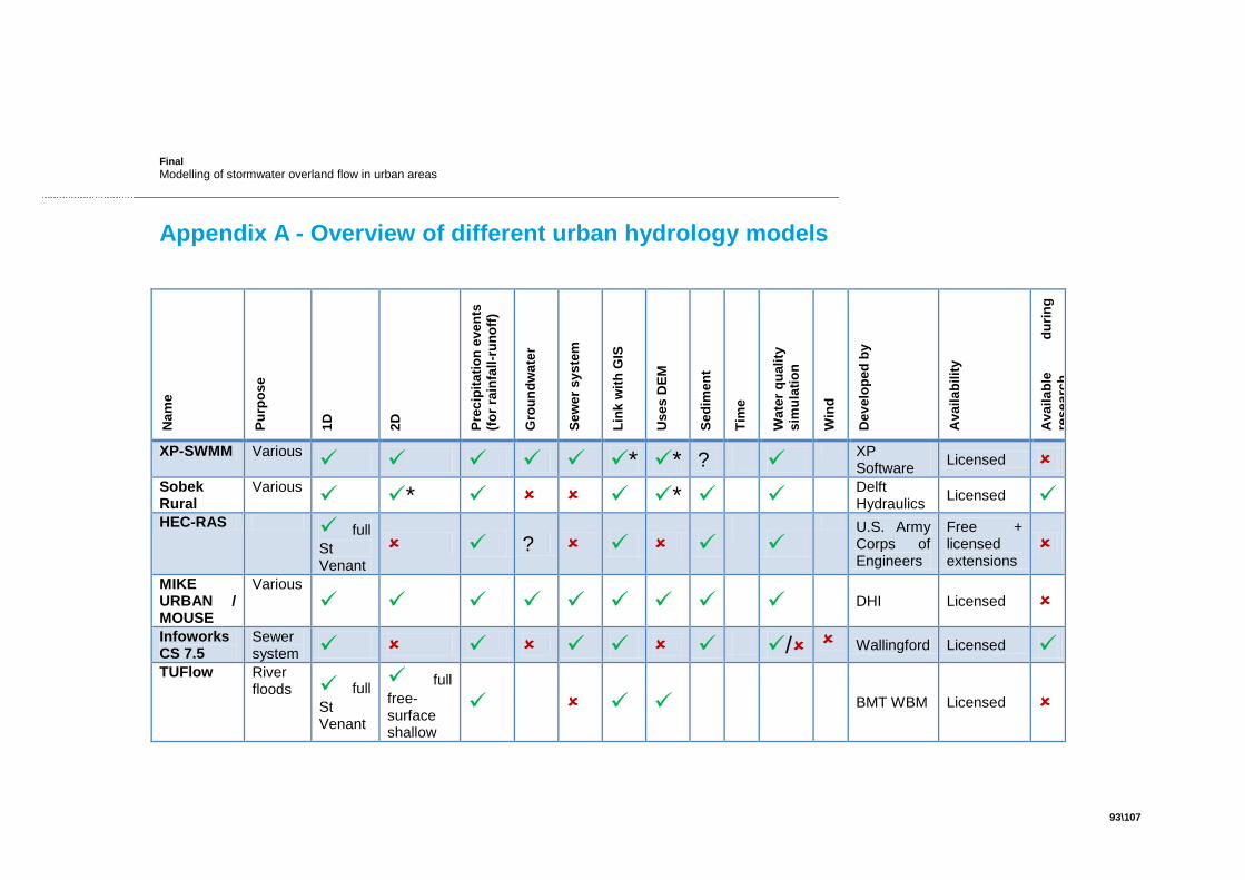
Final
Modelling of stormwater overland flow in urban areas
93\107
Appendix A - Overview of different urban hydrology models
Nam
e
Pu
rpo
se
1D
2D
Pre
cip
ita
tio
n e
ve
nts
(fo
r ra
infa
ll-r
un
off
)
Gro
un
dw
ate
r
Se
we
r s
ys
tem
Lin
k w
ith
GIS
Use
s D
EM
Se
dim
en
t
Tim
e
Wa
ter
qu
ali
ty
sim
ula
tio
n
Win
d
Dev
elo
pe
d b
y
Ava
ila
bilit
y
Ava
ila
ble
d
uri
ng
res
ea
rch
XP-SWMM Various * * ?
XP Software
Licensed
Sobek Rural
Various * *
Delft Hydraulics
Licensed
HEC-RAS full
St Venant
?
U.S. Army Corps of Engineers
Free + licensed extensions
MIKE URBAN / MOUSE
Various
DHI Licensed
Infoworks CS 7.5
Sewer system / Wallingford Licensed
TUFlow River floods full
St Venant
full
free-surface shallow
BMT WBM Licensed

Final
Modelling of stormwater overland flow in urban areas
94\107
water eq.
DUFlow * *
Stowa Licensed RMA2
Navier-Stokes eq.
U.S. Army Corps of Engineers
Licensed
TELEMAC-2D
Full
2D St. Venant equations or shallow water eq.
?
? freeware ?
LISFLOOD FP
River flood only
main channel
diffusion eq. for floodplain
EU-Joint Research Centre, runs in PCRaster
Non-commercial only
WOLK Surface runoff / Tauw
Private application
Wodan Surface runoff / Grontmij
Private application
PCRaster Various
Utrecht University
Freeware + licensed extensions
?
* Depending on the which extensions of the model are used.

Final
Modelling of stormwater overland flow in urban areas
95\107
Appendix B – Interview questions
Eerst algemeen: - Hoe lang kent u Tauw al/ hoeveel projecten heeft u ongeveer al met ze uitgevoerd? ->
expertise/beeld van Tauw bepalen - Hoe lang bent u zelf al bezig met stedelijk waterbeheer? -> expertise bepalen - Hoe is de samenwerking met Tauw bij het WOLK project verlopen. -> beeld van Tauw
bepalen Inzoomen op het project:
- Zijn er tijdens het project zaken anders gegaan dan u zou willen? Hoe kan Tauw hierin de aanpak veranderen?
- Wat waren de vragen die de gemeente van tevoren had met betrekking tot wateroverlast?
- Zijn alle vragen die de gemeente had beantwoord met de WOLK analyse? Wat wel en wat niet?
Inzoomen op WOLK: - Vond u de resultaten voldoende nauwkeurig? - Vind u dat het gebruik van WOLK terecht was? Met andere woorden, is WOLK gebruikt
voor het juiste doel? - Vind u dat er nog zaken toegevoegd moeten worden aan WOLK
(hierbij is te denken aan riolering, grondwater, etc.) - Wat vind u van de prijs/kwaliteit verhouding van WOLK? - In WOLK worden alleen extreme buien gebruikt als invoer. Wat vind u hiervan? Vind u
het nuttiger als er exteme buien of ontwerpbuien (bui08/bui10) worden gebruikt? - Tussen de extreme buien en ontwerpbuien zit een gat met buien waarvan de
herhalingstijd van ongeveer 10 a 75 jaar hebben. Vind u het interessant om te weten wat het effect zou zijn van deze buien, of vind u een extreme bui (100jr) voldoende informatie geven?
- Wat wordt er gedaan met de resultaten van WOLK? Bijv als communicatie/bewustwordingsmiddel of echt om op detail niveau maatregelen te ontwerpen en deze uit te voeren?
- Met een analyse van de WOLK resultaten zijn oplossingen voor de wateroverlast te bedenken. Zijn er naast WOLK resultaten nog meer gegevens nodig om ook daadwerkelijk oplossingen te kunnen implementeren? Welke dan?
- Vind u dat deze gegevens ook al in de analyse van WOLK meegenomen moeten worden?
- Hoe denkt u (de resultaten van) WOLK in de toekomst te gaan gebruiken?


Final
Modelling of stormwater overland flow in urban areas
97\107
Appendix C – AHN data
The first series of surface elevation measurements has been carried out in the Netherlands between 1997 and 2003. These first measurements provided a DEM, the AHN-1, with at least one measurement point per 16m
2 but up to 1m
2. A vertical accuracy of 20cm in 68% of the
measurements could be assured (Van der Zon, 2010). The measurements from this period are outdated on some locations: new housing development have occurred, riverbeds have been changed, etc. Furthermore new measurements techniques have come available. Therefore, in 2007 a new measurement round started with the goal of creating an even more accurate DEM: the AHN-2. This round is expected to be complete in 2012, and the result will be a DEM with raster size 0.5x0.5 meter and a 10cm vertical accuracy in 68% of the cases. The goal is to repeat the measurements of the AHN each 5 years so the data is kept up to date. An improvement of the measuring techniques in combination with repeated measurements can be used for analysis such as ground subsidence. An overview of the measurement accuracy of both the AHN-1 and AHN-2 can be found in the table below.
Table C.0.1. Measurement errors of AHN-1 and AHN-2. Adapted from Van der Zon (2010)
AHN-1 AHN-2 Systematic error 5 cm 5 cm
Stochastic error 15 cm 5 cm
The accuracy of >68.2% (systematic + 1*stochatic error) 20 cm 10 cm
The accuracy of >95.4% (systematic + 2*stochatic error) 35 cm 15 cm
The accuracy of >99.7% (systematic + 3*stochatic error) 50 cm 20 cm
An issue which influences the amount of available data points per square meter is the reflection ability of the surface. Surfaces like asphalt roads and black roof tiles don‟t reflect the laser beam. Another issue that influences the measurement uncertainty are data gaps next to tall buildings. The survey is conducted from the air with 100m wide beams. Especially in cities with tall buildings the gap can be in the order of several meters. The effect is minimized by using a narrower beam and altering flight level. The surface level in the gaps is interpolated during data processing.
Figure C.0.1.Cause of measurements gaps next to tall buildings
The gaps next to tall buildings are mostly walkways, which are important in the modelling of urban surface runoff. The possibility of measurement errors in cities with tall buildings should be kept in mind.

Final
Modelling of stormwater overland flow in urban areas
98\107
The measurements with laser altimetry provide surface elevations (Digital Surface Model (DSM)). This is not the same as ground elevations: Digital Elevation Model (DEM) or Digital Terrain Model (DTM). Buildings, cars, vegetation, etc stand on top of the ground, thus obscuring the measurement of the „real‟ terrain elevation. The measurements are therefore filtered for any items on top of the surface. In order to minimize the errors due to vegetation, the surveys are only conducted between December 1st and March 31st, because during this period the amount of vegetation density is minimal. Errors might also occur due to snow, tidal influences or flooding. Tidal influences are minimized by surveying only in a two-hour window around low tide. Floodings in winter period are mainly found on agricultural areas, so this is not an issue for urban areas.

Final
Modelling of stormwater overland flow in urban areas
99\107
Appendix D – section of DEM Apeldoorn
Figure D.0.1. Section of DEM AHN-2 Apeldoorn.

Final
Modelling of stormwater overland flow in urban areas
100\107
Appendix E – General St. Venant equations
The general St. Venant equations are: Continuity
(C.1)
Momentum
(C.2)
= discharge at the section (m
3/s)
= cross-sectional area of flow (m2)
= width of the top of the section
= lateral flow per unit length of channel (m3/s/m)
= position of the section measured from the upstream end (m)
= depth of flow (m) = acceleration due to gravity (m/s
2)
= time (s)
= sin = = bed slope
= energy loss/unit length of channel/unit weight of fluid. can be either Chezy or Manning.

Final
Modelling of stormwater overland flow in urban areas
101\107
Appendix F – Catchment representation
Table F.0.1 Overview of the geometry of four process-oriented rainfall runoff models (Grayson & Blöschl,
2000; Huisman & de By, 2009)
Approach Schematic diagram Advantages Disadvantages
Regular tessellation: grids
DEMs are often available as grids Computationally simple to set up
dynamic models Simple to overlay other spatial
information
Flow direction not straightforward to define: only in 8 directions.
Uniform raster size can increase runtime
Contours and streamlines
More naturally suited to the routing of surface flow
Able to assume 1D flow in each element
Does not allow flow to cross streamline
Few models use this structure, because dynamic modelling is challenging
Triangulated Irregular Network (TIN) facets
Most efficient form of surface definition – least number of elements for most terrain detail
The problem with TINs for distributed modelling is that flow paths are difficult to represent
Few models are designed for this structure
Data type is not common, and difficult to overlay other spatial data.
There are many different TINs possible for a given input set of points

Final
Modelling of stormwater overland flow in urban areas
102\107
Conceptual elements of hillslopes and stream segments
Based on the assumption that it is only those features preserved in the elements (such as: average slope, flow path length, area) that are important to model response
Able to assume 1D flow in each element
Smaller number of elements required and thus a faster model run time
Manually discretisation required Uncertainty about the
validity of the main assumptions I some applications

Final
Modelling of stormwater overland flow in urban areas
103\107
Appendix G – Manning’s n coefficient
Table G.0.1. Manning's n for Channels (Chow, 1959).
Type of Channel and Description Minimum Normal Maximum
Main Channels
clean, straight, full stage, no rifts or deep pools 0.025 0.030 0.033
very weedy reaches, deep pools, or floodways with heavy stand of timber and underbrush
0.075 0.100 0.150
Floodplains
short grass 0.025 0.030 0.035
high grass 0.030 0.035 0.050
Cultivated areas: no crop 0.020 0.030 0.040
Cultivated areas: mature row crops 0.025 0.035 0.045
Cultivated areas: mature field crops 0.030 0.040 0.050
scattered brush, heavy weeds 0.035 0.050 0.070
light brush and trees, in winter 0.035 0.050 0.060
light brush and trees, in summer 0.040 0.060 0.080
medium to dense brush, in winter 0.045 0.070 0.110
medium to dense brush, in summer 0.070 0.100 0.160
Trees: dense willows, summer, straight 0.110 0.150 0.200
cleared land with tree stumps, no sprouts 0.030 0.040 0.050
Excavated or Dredged Channels
clean, recently completed 0.016 0.018 0.020
with short grass, few weeds 0.022 0.027 0.033
Dragline-excavated or dredged: no vegetation 0.025 0.028 0.033
Dragline-excavated or dredged : light brush on banks 0.035 0.050 0.060
dense weeds, high as flow depth 0.050 0.080 0.120
clean bottom, brush on sides 0.040 0.050 0.080
Lined or Constructed Channels
Concrete 0.011 0.013 0.015
Sewer with manholes, inlet, etc., straight 0.013 0.015 0.017
Brick: glazed 0.011 0.013 0.015
Brick: in cement mortar 0.012 0.015 0.018
Dressed ashlar/stone paving 0.013 0.015 0.017
Asphalt: smooth 0.013 0.013
Asphalt: rough 0.016 0.016


Final
Modelling of stormwater overland flow in urban areas
105\107
Appendix H – Test results of Manning-based model
Figure H.1. Test 1

Final
Modelling of stormwater overland flow in urban areas
106\107
Figure H.2. Test 3

Final
Modelling of stormwater overland flow in urban areas
107\107
Figure H.3. Test 4