modelling of solvation thermodynamics by using a combination of
TRANSCRIPT
Modelling of Solvation Thermodynamics byUsing a Combination of Reference InteractionSite Model Theory and Multi-grid Numerical
Methods
Volodymyr Sergiievskyi
Department of Physics; Scottish Universities Physics Alliance
A thesis presented in fulfilment of the requirements for the degree of
Doctor of Philosophy
2012

This thesis is the result of the author’s original research. It has been composed by the
author and has not been previously submitted for examination which has led to award of a
degree.
The copyright of this thesis belongs to the author under the terms of the United Kingdom
Copyright Acts as qualified by University of Strathclyde Regulation 3.50. Due acknowledgement
must always be made of the use of any material contained in, or derived from, this thesis.
Signed:
Date:

To my wolverine
Abstract
Solvation Free Energy (SFE) is a fundamental property in chemical physics. It describes sova-
tion behavior of substances in a liquid media and has many important applications in solution
chemistry, biophysics, pharmaceutics, medicine, and environmental sciences. In many appli-
cations (for example screening of drug-candidate databases in drug-discovery process) it is
important to have a fast and accurate method for solvation free energy calculation. In this
thesis two new methods for fast and accurate SFE calculations are proposed. The methods
combine a theoretical basis of the integral equation theory of liquids with advanced computa-
tional techniques. The theoretical part of the methods is based on the Reference Interaction
Site Model (RISM) and the three-dimensional RISM (3DRISM) molecular theories and semi-
empirical models for SFE calculations. The computational part of the methods is based on
the multi-grid scheme which drastically increase the computational performance. Additional
investigations of speed and accuracy of calculations are performed to determine the optimal
parameters of the methods which allow one to calculate the SFE with the required accuracy
with the minimal computational expenses. The methods are benchmarked on extended sets
of small organic and drug-like compounds. It is shown that both (RISM and 3DRISM-based)
methods can be successfully used for SFE calculations. It was shown that the parameters of
the methods are transferable between different classes of compounds. The average computa-
tion time per typical drug-like compound of about 20 atoms is 17 seconds for the RISM-based
method and about 3.5 minutes for the more accurate 3DRISM-based method.
i
Acknowledgements
I would like to acknowledge my supervisor, Prof. Maxim Fedorov for organizing of my PhD
research. I am thankful to Prof. Gennady N. Chuev for organizing the course of lectures in
Statistical Mechanics in the Max Planck Institute for Mathematics in the Sciences which I
attended during my PhD study. These lectures helped my to understand the basics of the
Integral Equation Theory of Liquids which is the theoretical base of my current research. I am
deeply grateful to Dr. Andrey I. Frolov for fruitful discussions which helped me a lot to improve
my understanding of physical chemistry and statistical physics. I would like to thank Dr.
Ekaterina Ratkova for useful advices and consultations in Quantum Mechanical calculations. I
am grateful to Wolfgang Hackbusch for insightful discussions on different aspects of multi-grid
mathematical background. I would like to acknowledge Dr. David S. Palmer for productive
collaboration.
I would like to acknowledge financial support of Max Planck Society, University of Strath-
clyde, Deutsche Forschungsgemeinschaft (DFG) - German Research Foundation, Research Grant
FE 1156/2-1 and REA Research Executive Agency, Grant No. 247500 ”BioSol”, Programme:
FP7-PEOPLE-2009-IRSES.
ii
Contents
1 Introduction 1
1.1 Goals . . . . . . . . . . . . . . . . . . . . . . . . . . . . . . . . . . . . . . . . . . 5
1.2 Structure of the thesis . . . . . . . . . . . . . . . . . . . . . . . . . . . . . . . . 6
2 Statistical Mechanical background 7
2.1 Systems under investigation . . . . . . . . . . . . . . . . . . . . . . . . . . . . 7
2.2 Phase space. Ensemble. Micro-canonical ensemble . . . . . . . . . . . . . . . . 8
2.3 Continuity equation . . . . . . . . . . . . . . . . . . . . . . . . . . . . . . . . . 9
2.4 Liouville equation . . . . . . . . . . . . . . . . . . . . . . . . . . . . . . . . . . . 12
2.5 Gibbs distribution . . . . . . . . . . . . . . . . . . . . . . . . . . . . . . . . . . . 13
2.6 Entropy . . . . . . . . . . . . . . . . . . . . . . . . . . . . . . . . . . . . . . . . 17
2.7 Temperature . . . . . . . . . . . . . . . . . . . . . . . . . . . . . . . . . . . . . . 19
2.8 Free Energy . . . . . . . . . . . . . . . . . . . . . . . . . . . . . . . . . . . . . . 21
2.9 Grand Canonical Ensemble . . . . . . . . . . . . . . . . . . . . . . . . . . . . . . 22
2.10 Solubility and Solvation Free energy . . . . . . . . . . . . . . . . . . . . . . . . . 24
3 Integral Equation Theory of Liquids. RISM and 3DRISM 26
3.1 System under investigation . . . . . . . . . . . . . . . . . . . . . . . . . . . . . . 26
3.2 Configurational integral . . . . . . . . . . . . . . . . . . . . . . . . . . . . . . . 27
3.3 Density distribution functions . . . . . . . . . . . . . . . . . . . . . . . . . . . . 30
3.4 Free Energy functional . . . . . . . . . . . . . . . . . . . . . . . . . . . . . . . . 32
3.4.1 Minimization property of the free energy functional . . . . . . . . . . . . 33
3.5 Free Energy Functional of the Ideal Gas . . . . . . . . . . . . . . . . . . . . . . 34
3.6 Functional derivatives . . . . . . . . . . . . . . . . . . . . . . . . . . . . . . . . . 36
3.7 Direct correlation functions . . . . . . . . . . . . . . . . . . . . . . . . . . . . . 37
3.8 Long-range approximation of direct correlation functions . . . . . . . . . . . . . 39
3.9 Ornstein-Zernike equation . . . . . . . . . . . . . . . . . . . . . . . . . . . . . . 40
3.10 Closure relation . . . . . . . . . . . . . . . . . . . . . . . . . . . . . . . . . . . . 43
3.11 Reference interaction site model . . . . . . . . . . . . . . . . . . . . . . . . . . . 45
iii
iv CONTENTS
3.12 Closure relation for the RISM equations . . . . . . . . . . . . . . . . . . . . . . 49
3.13 RISM equations in a Fourier space . . . . . . . . . . . . . . . . . . . . . . . . . 50
3.14 Reducing the RISM equations to the system of one-dimensional equations . . . 51
3.15 Bessel-Fourier transformation . . . . . . . . . . . . . . . . . . . . . . . . . . . . 51
3.16 Inverse Bessel-Fourier transformation . . . . . . . . . . . . . . . . . . . . . . . . 52
3.17 RISM equations in a matrix representation . . . . . . . . . . . . . . . . . . . . . 55
3.18 3DRISM equations . . . . . . . . . . . . . . . . . . . . . . . . . . . . . . . . . . 57
4 Solvation Free Energy calculation in RISM and 3DRISM 59
4.1 Thermodynamic integration . . . . . . . . . . . . . . . . . . . . . . . . . . . . . 59
4.2 Thermodynamic integration in the RISM approximation . . . . . . . . . . . . . 60
4.3 RISM-HNC Solvation Free Energy expression . . . . . . . . . . . . . . . . . . . 61
4.4 Other Solvation Free Energy Expressions . . . . . . . . . . . . . . . . . . . . . . 64
4.5 Semi-Empirical Solvation Free Energy expressions . . . . . . . . . . . . . . . . . 67
4.6 Models based on the partial molar volume correction . . . . . . . . . . . . . . . 69
5 RISM Multi-grid algorithm 71
5.1 Iterative representation of RISM equations . . . . . . . . . . . . . . . . . . . . . 71
5.1.1 Indirect correlation functions . . . . . . . . . . . . . . . . . . . . . . . . 71
5.1.2 RISM equations for short-range functions . . . . . . . . . . . . . . . . . . 73
5.1.3 RISM equations in a recurrent form . . . . . . . . . . . . . . . . . . . . . 74
5.2 Discretization of the problem . . . . . . . . . . . . . . . . . . . . . . . . . . . . 75
5.3 Picard iteration . . . . . . . . . . . . . . . . . . . . . . . . . . . . . . . . . . . . 77
5.4 Moving between the grids . . . . . . . . . . . . . . . . . . . . . . . . . . . . . . 78
5.5 Nested Picard iteration . . . . . . . . . . . . . . . . . . . . . . . . . . . . . . . . 79
5.6 Two- and multi-grid iteration . . . . . . . . . . . . . . . . . . . . . . . . . . . . 80
5.7 Nested multi-grid . . . . . . . . . . . . . . . . . . . . . . . . . . . . . . . . . . . 84
5.8 Optimal number of coarse-grid steps . . . . . . . . . . . . . . . . . . . . . . . . 85
5.9 Optimal parameters for calculations . . . . . . . . . . . . . . . . . . . . . . . . . 86
5.10 Optimal grid parameters . . . . . . . . . . . . . . . . . . . . . . . . . . . . . . . 88
5.11 The RISM-MOL solver . . . . . . . . . . . . . . . . . . . . . . . . . . . . . . . . 89
5.12 Performance of the algorithm . . . . . . . . . . . . . . . . . . . . . . . . . . . . 92
5.13 Calculation of Hydration Free Energy of drug-like compounds . . . . . . . . . . 93
5.14 Conclusions . . . . . . . . . . . . . . . . . . . . . . . . . . . . . . . . . . . . . . 101
6 3DRISM multi-grid algorithm 102
6.1 Iterative solution of the 3DRISM equations . . . . . . . . . . . . . . . . . . . . 102
CONTENTS v
6.2 DIIS and MDIIS iteration . . . . . . . . . . . . . . . . . . . . . . . . . . . . . . 105
6.3 Multi-grid . . . . . . . . . . . . . . . . . . . . . . . . . . . . . . . . . . . . . . . 106
6.4 Finding the optimal grid parameters . . . . . . . . . . . . . . . . . . . . . . . . 111
6.5 Dependencies of the computational time on the η and λ parameters . . . . . . . 111
6.6 Performance of the solver . . . . . . . . . . . . . . . . . . . . . . . . . . . . . . . 112
6.7 Benchmarks on a large set of molecules . . . . . . . . . . . . . . . . . . . . . . . 116
6.8 Conclusions . . . . . . . . . . . . . . . . . . . . . . . . . . . . . . . . . . . . . . 121
7 Conclusions and further work 124
7.1 Conclusions . . . . . . . . . . . . . . . . . . . . . . . . . . . . . . . . . . . . . . 124
7.2 Future work . . . . . . . . . . . . . . . . . . . . . . . . . . . . . . . . . . . . . . 126
7.2.1 Approaches for solving 6D OZ equation . . . . . . . . . . . . . . . . . . . 126
7.2.2 Proper closure for the OZ equations . . . . . . . . . . . . . . . . . . . . . 127
7.2.3 Finding of the most probable binding positions of solvent molecules . . . 129
7.3 Concluding remarks . . . . . . . . . . . . . . . . . . . . . . . . . . . . . . . . . . 131
A Low rank representation of multidimensional functions 133
List of Figures
5.1 Dependencies of the RISM SFE error on the grid step . . . . . . . . . . . . . . . 88
5.2 Dependencies of the RISM SFE error on the cutoff distance . . . . . . . . . . . . 89
5.3 Speedup of different RISM solvers . . . . . . . . . . . . . . . . . . . . . . . . . . 90
5.4 Speedup with regards to the nested Picard RISM solver . . . . . . . . . . . . . . 90
6.1 Buffer and spacing . . . . . . . . . . . . . . . . . . . . . . . . . . . . . . . . . . 104
6.2 Constant and variable decay factor in 3DRISM multi-grid iterations . . . . . . . 109
6.3 Dependency of the error on the grid spacing . . . . . . . . . . . . . . . . . . . . 112
6.4 Dependency of the errors on the buffer . . . . . . . . . . . . . . . . . . . . . . . 113
6.5 Dependency of the computation time of lambda for MG-Picard . . . . . . . . . . 113
6.6 Dependency of the computation time of lambda for MG-MDIIS . . . . . . . . . 114
6.7 Dependency of the computation time on eta . . . . . . . . . . . . . . . . . . . . 114
6.8 Speedup of the 3DRISM calculations . . . . . . . . . . . . . . . . . . . . . . . . 115
6.9 Benchmarking of the MG-MDIIS algorithm . . . . . . . . . . . . . . . . . . . . . 117
6.10 Correlations of experimental and calculated SFEs . . . . . . . . . . . . . . . . . 123
7.1 Water binding sites for the deprotonated benzoic acid in water . . . . . . . . . . 129
7.2 Water binding sites for the α-cyclodextrin in water . . . . . . . . . . . . . . . . 130
vi

List of Tables
5.1 Comparison of the multi-grid and the nested Picard iteration . . . . . . . . . . . 91
5.2 Compounds in the SAMPL1 set . . . . . . . . . . . . . . . . . . . . . . . . . . . 93
5.3 Results of the RISM SFE calculations . . . . . . . . . . . . . . . . . . . . . . . . 99
5.4 Results of the RISM parameterization . . . . . . . . . . . . . . . . . . . . . . . . 100
5.5 Parameterization coefficients for the RISM expressions . . . . . . . . . . . . . . 100
6.1 Computational expenses for 3DRISM calculations . . . . . . . . . . . . . . . . . 115
6.2 Molecules in the training set . . . . . . . . . . . . . . . . . . . . . . . . . . . . . 117
6.3 Molecules in the test set . . . . . . . . . . . . . . . . . . . . . . . . . . . . . . . 118
vii

List of abbreviations
1D one dimensional3D three dimensional6D six dimensionalB3LYP Becke, three-parameter, Lee-Yang-Parr (method)CHELPG CHarges from Electrical Potential Grid-based methodDIIS Direct Inverse in the itarative subspace (method)DME DiMethy EtherFFT Fast Fourier TransformGB Generalized-Born (equation)GF Gaussian Fluctuations (expression)GMRES Generalized Minimal RESidual (method)HFE Hydration Free EnergyHNC Hyper Netted Chain (closure)IETL Integral Equation Theroy of LiquidsKH Kovalenko-Hirata (closure)MDIIS Modified DIIS (method)MD Molecular DynamicsMG Multi-grid (method)MOZ Molecular Ornstein Zernike (equation)MSPCE, MSPC/E Modified SPC/E (water model)NR Newton-Raphson (method)OPLS Optimized Potentials for Liquid SimulationsOZ Ornstein-Zernike (euqation)PB Poisson-Boltzmann (equation)PMV Partial Molar VolumePW Partial Wave (expression)RISM Reference Interaction Site ModelRMSD Root Mean Square DeviationSCF Self-Consisten FieldSFE Solvation Free EnergySPCE, SPC/E Simple Point Charge, Extended (water model)UC Universal Correction (method)

Chapter 1
Introduction
Eo quod in multa sapientia multa sit indignatio
et qui addit scientiam addat et laborem
Ecclesiastes 1:18
Accurate calculation of the hydration free energies of organic molecules is a long-standing
challenge in computational chemistry and is important in many aspects of research in the phar-
maceutical and agrochemical industries. For example, many of the pharmacokinetic properties
of potential drug molecules are defined by their in vivo solvation and acid-base behavior, which
can be estimated from their hydration free energies. [1, 2, 3, 4, 5, 6, 7]
Commonly used methods to calculate hydration free energy may be categorized as either
explicit or implicit solvent models. In the first approach, each solvent molecule is included
explicitly and molecular simulation methods are used to sample their conformational freedom
[1, 2, 8, 9, 10, 11, 12, 13]. In the second approach, the implicit effect of solvent on solute is
included by solving either the Poisson-Boltzmann (PB) or Generalized-Born (GB) equation
[14, 15, 16, 17, 18]. While explicit solvent methods are more scientifically rigorous, implicit
models are often preferred because they are less computationally expensive. Explicit models
can be successfully used in scientific investigations. However in many cases they are too slow to
be used in practical industrial applications. One of applications there the speed of calculations
is critical is a drug-discovery industry, where one need to filter large databases of drug-like
candidates which can contain thousands and millions of compounds. For such kind of appli-
cations only implicit methods can be applied. However not all of the implicit methods are
accurate enough. In some cases the errors of Solvation Free Energy (SFE) predictions can be of
2.5-3.5 kcal/mol, which equates to a ∼ 2 log unit error in the related pharmacokinetic property
(estimated from ∆Gsolv = −RT lnK) and is not enough for chemical applications[19, 20, 21]
. Integral Equation Theory of Liquids (IETL) is an alternative framework for the calculation
of hydration free energies [22, 23, 24]. Unlike PB or GB methods, it retains information about
1

2 CHAPTER 1. INTRODUCTION
the solvent structure (in terms of density correlation functions), but estimates the solute chem-
ical potential without long molecular dynamics (MD) or Monte Carlo (MC) simulations. At
present, there are several approaches based on integral equations. The six-dimensional molec-
ular Ornstein–Zernike (MOZ) theory is used to calculate the three-dimensional (3D) hydration
structure in molecular liquids.[25, 26] The site–site Ornstein–Zernike (SSOZ) integral equation
is used to calculate the properties of complex solute-solvent systems in the Reference Interac-
tion Site Model (RISM) formalism developed by Chandler and Anderson and others [27, 28, 29].
The theory has been applied successfully to calculation of the structural and thermodynamic
properties of various chemical and biological systems [30, 31, 32, 33, 34, 35, 36, 37, 38, 39]. Re-
cently Integral Equation Theory of Liquids was also successfully applied to some biochemical
applications [40, 41, 42, 43, 44, 45].
In terms of computational expenses IETL offers a compromise between computationally ex-
pensive fully-atomistic simulations [46, 47, 48] and rather approximate continuum electrostatic
models [17, 14, 49]. To solve an OZ equation one should complete this by a closure relation
which makes the system OZ+closure solvable. However, the closure relation incorporates a so-
called bridge function, which is practically incomputable due to the infinite number of terms in
the exact representation of this functional[50, 51]. Therefore, in practice one uses approximate
closure relations [52, 24].
Nowadays, only few methods exist for solving the six-dimensional MOZ equation. This
can be explained by the computational complexity of the problem. Although with modern
computers straightforward calculations on the six-dimensional grid with moderate resolution
are already feasible they are still extremely computationally demanding[53]. Other class of
methods uses low-rank decomposition of the correlation functions. In that case the translational
and rotational components are separated and basis functions are used for representation of the
rotational degrees of freedom. Typically, for the rotational degrees of freedom the basis set of
rotational invariants is used [54, 55]. In some cases some advanced techniques like hierarchical
matrix decomposition, could be used to reduce the computational complexity of the method[56].
For additional discussion of the computational complexity of operations in different the low-rank
formats one may refer to the appendix A of this thesis.
Despite the recent progress in the six-dimensional MOZ theory, for a time being it was tested
only for small and simple molecules only. This can be explained by the high computational cost
of solution of six-dimensional problem with reasonable accuracy. In practical applications one
usually uses simplified models and the Reference Interaction Sites Model (RISM) is one of the
most popular among them. The main assumption in the model is that the molecular correlation
functions can be represented as a sum of spherically symmetric functions corresponding to the
selected parts of the molecule (so-called sites). As a result, the operations with the spherically

3
symmetric functions can be reduced to the operations with only their radial parts and that
makes the RISM integral equations effectively one-dimensional. The six-dimensional MOZ
equation is replaced by a set of one-dimensional non-linear integral equations. Despite of its
relative simplicity RISM-based methods have several important applications. RISM equations
can be self-consistently used to introduce an implicit solvent model in Quantum mechanical
calculations (RISM-SCF method) [57, 58, 59, 60, 61]. From a computational point of view it
is relatively inexpensive to solve the RISM equations numerically for small molecular solutes
(< 102 atoms) with modern computers; and, typically, solutions of the RISM equations give
a qualitatively correct description of the solvent structure around the solute. In addition,
RISM theory gives end-point expressions for solvation free energy calculation which simplifies
calculations [52, 62]. We note though that the original formulae for SFE calculations [52, 62]
provide only qualitative predictions of trends in the differences of SFEs for different compounds
[63]. Recently there were proposed several methods for parameterizing RISM solvation free
energy calculations that predict SFEs with the accuracy of around 1 kcal/mol [63, 64, 65, 66, 67].
However, decomposition of molecular functions to site-site spherically symmetric functions
leads to inaccurate representation of molecular structure. Therefore, a considerable number
of empirical corrections is necessary to achieve a good accuracy of predictions.
Another approximation of the Ornstein-Zernike equation is the three-dimensional RISM
(3DRISM) [68, 69] where a solute molecule is represented as a three dimensional object. The
3DRISM operates with a set of three-dimensional equations and that model provides bet-
ter spatial description of solute-solvent correlations than the RISM. The 3DRISM method
is currently widely used in biochemical applications for description of solvation properties of
biomolecules [70, 42, 71, 72]. As it was recently shown, a 3DRISM-based method (so-called
Universal Correction (UC) method) accurately predicts thermodynamic parameters of hydrated
organic molecules including drug-like molecules[73, 74]. However, for small molecules, numerical
solution of the multidimensional 3DRISM equations requires significantly more computational
time than solution of the RISM equations [74]. High computational expenses of 3DRISM cal-
culations is a real bottleneck of this method that inhibits wider applications of this technique.
Coming back to the history of the IETL, the first algorithm used for solving OZ-like integral
equations was presumably the Picard iteration method [22]. This method is easy to implement.
However, it has a comparably low convergence rate. One may use faster convergent schemes,
such as the Newton-Raphson (NR) iteration [75], NR-GMRES algorithm [76], method of direct
inversion in iterative subspace(DIIS)[77] , combination of modified NR and DIIS iteration[78]
or vector extrapolation technique [79] . For the 3DRISM equations it was recently proposed to
use the Modified DIIS (MDIIS) method [77]. Recently an efficient 3DRISM equations solver
which uses the MDIIS algorithm was implemented in the Amber molecular modeling software

4 CHAPTER 1. INTRODUCTION
[71]. However, for the grids with a large number of points and/or molecular systems with a
large number of interacting sites these methods are computationally expensive. An alternative
way to increase efficiency is to use a multi-scale approach. Commonly used approach is a
combined two-level NR-Picard scheme, so-called Gillan method [80] . Similar two-level NR-
Picard schemes are used also in the Labık-Malijevsky-Vonka method [81, 82] or wavelet-based
methods [83, 84, 85, 56]. Although two-level methods give an essential improvement with
respect to the Picard iteration, two level approaches have limitations because fine-grid and
coarse-grid resolutions cannot differ too much. Multi-level methods can be used to overcome
these limitations. Recently an effective multilevel NR-GMRES algorithm has been applied to
the problem [86]. This algorithm does not have such restrictions as the two-level methods;
NR-GMRES algorithm is a fast convergent method and it needs much less iteration steps to
converge than the Picard iteration. However, faster convergence in terms of number of iteration
steps does not necessarily mean better performance in terms of computer time. The Newton-
Raphson method requires computation and inversion of a Jacobian matrix of size N × N ,
where N is a number of discretization points on the coarse grid (typically N ≈ 50 − 100).
Although the implementation in the work [86] does not require inversion of a Jacobian matrix it
nevertheless requires operations with matrices of size N ×N which demand additional storage
and computational time and make each iteration step computationally expensive. For the
RISM, where number of coarse-grid points N is not very large these additional computational
expenses for each iteration step can be compensated with much smaller number of iteration
steps. However, it is not so for the three dimensional problem where the number of grid points
grows cubically with respect to the one-dimensional problem.
Despite the fact that many methods use sophisticated algorithms to enhance computational
performance often these methods do not fully exploit the advantages of the multi-scale approach.
The multi-grid method is a multi-scale technique in a sense that the iteration makes use of
different grids (different discretization levels) and is more efficient than simple nested iteration
schemes [87]. The multi-grid scheme is not restricted to a specific type of iterations and can
be applied to any kind of iteration process. Multi-grid methods are actively used in different
applications in computational chemistry [88, 89, 90, 91]. Recently it has been shown that a
multi-grid technique incorporating the Picard iteration for 1D OZ equation for simple liquids
is able to improve the computational efficiency of the algorithm up to the several dozen times
[92].
In our work we propose algorithms for solving RISM and 3DRISM equations based on the
multi-grid scheme. We are focused on the practical application of the algorithms to the solvation
free energy calculations. We perform additional investigations to determine some guidelines for
choosing algorithms’ parameters which are optimal for the solvation free energy calculations.

1.1. GOALS 5
We compare the numerical performance of the proposed RISM multi-grid algorithm to the
one-grid Picard iteration and to the nested Picard iteration methods. The general multi-grid
framework for solving equations allows one to combine this method with other different numer-
ical solvers. In our work we investigate the performance of two modifications of the 3DRISM
multi-grid algorithm where the multi-grid is combined with (i) the Picard iteration method
(MG-Picard); and (ii) with the MDIIS method (MG-MDIIS) respectively. By benchmarking of
these methods on a set of model compounds we determine the optimal grid parameters for sol-
vation (hydration) free energy calculations. We test the numerical performance of the proposed
methods and compare it to the performance of the standard Picard iteration method and the
MDIIS method.
To test the effectiveness of the proposed methods we benchmark the speed and accuracy
of the methods on extended sets of organic compounds. To test the effectiveness of developed
RISM multi-grid algorithm for calculation of SFE of bioactive drug-like molecules we use the
set of 63 compounds from Ref. [93]. In our work we perform the RISM calculations for 63
compounds from Ref. [93], discuss efficiency of different RISM-SFE expressions and perform
a parameterization which allow to improve computational results. For testing of the 3DRISM
algorithm the set of 99 organic compounds from the paper [74] was chosen. Firstly, we test
computational performance of the algorithm. Then we test the accuracy of the SFE calculations
with the Universal Correction model (UC) as proposed in [64]. To check the accuracy of the free
energy results we calculate the correlation coefficient and root mean square deviation between
calculated and experimental data.
1.1 Goals
The main goal of the thesis is developing of fast and accurate methods for Solvation Free
Energy (SFE) calculations reliable for molecular biophysics and medicine. This goal poses
computational and theoretical challenges. On the one hand, in many cases it is critical to have
fast methods for SFE calculation. On the other hand, the method should provide a reasonable
accuracy of the SFE calculations to be useful for practical applications. To achieve the goal
the combination of RISM and 3DRISM molecular theories in combination with semi-empirical
SFE calculation methods is used in this work. The multi-grid technique is used to speed-up
RISM and 3DRISM calculations. The tasks of the current work are:
1. Developing of the fast multi-grid methods for solving of RISM and 3DRISM equations.
2. Investigation of the accuracy of different semi-empirical SFE expressions on the sets of the
compounds from different chemical classes, including drug-like polyfragment compounds.

6 CHAPTER 1. INTRODUCTION
3. Investigation of the computational errors and computational performance of the algo-
rithms and determining the optimal parameters for the fast and accurate calculations.
1.2 Structure of the thesis
The thesis consists of 7 chapters and appendix.
The first chapter is introduction.
In the chapter 2 some basic concepts of the statistical mechanics and thermodynamics are
described.
The chapter 3 contains description of the theoretical background of the integral equation
theory of liquids and Reference interaction site model(RISM) and three-dimensional RISM
(3DRISM), which are the theoretical base for the methods proposed in the current work.
In the chapter 4 the the ways to calculate the solvation free energy in the RISM and 3DRISM
approximations are discussed.
In the chapters 5 and 6 the RISM and 3DRISM multi-grid algorithms for calculation of
the solvation free energy are described. Descriptions of both methods have the same structure
which includes three parts: (i) description of the numerical method (ii) determining of the
optimal parameters of the method (iii) benchmarking of speed and accuracy of the method on
a set of organic compounds.
In the chapter 7 the perspectives of the theory are discussed and some preliminary results
of the ongoing research are described.
In the appendix the low-rank format for efficient operations with the multi-dimensional
functions is described.

Chapter 2
Statistical Mechanical background
In this chapter the basic concepts in statistical mechanics, such as ensemble average, partition
function, free energy etc are described. The chapter is mostly based on Refs. [94] and [95].
2.1 Systems under investigation
One of the main tasks of the statistical mechanics is description of common laws of the many
particle systems. Let there be N particles in the system, and each of the particles have m
degrees of freedom. Then the total number of degrees of freedom of the system is s = m · NAccording to the Hamilton’s equation the system which has s degrees of freedom can be de-
scribed by the s generalized coordinates (q1(t), . . . , qs(t)) and s generalized momenta compo-
nents (p1(t), . . . , ps(t)). For such a system the Hamiltonian equations hold [96]:
qi =∂H∂pi
pi = −∂H∂qi
i = 1 . . . s (2.1)
where pi = ∂pi/∂t, qi = ∂qi/∂t, H = H(p1, . . . , ps, q1, . . . , qs) is the Hamiltonian of the system.
If the Hamiltonian H is known the equations (2.1) can be solved numerically for any initial
conditions pi(t0) = p0i , qi(t0) = q0i , i = 1 . . . s which allows to predict the state of the system
at any moment t. Using this information it is possible to calculate the quantities of interest:
temperature, pressure, density, residence time etc. This approach is the base for Molecular Dy-
namics (MD) simulations. Despite of simplicity and universality of this method MD simulations
require comparably large computational resources. Today typical size of simulated systems is
only about 1000-10000 molecules and typical simulation time is 100 ns. The limit which can
be achieved with the modern computational resources lies at 106-107 molecules simulated for
1-2 µs.
7

8 CHAPTER 2. STATISTICAL MECHANICAL BACKGROUND
2.2 Phase space. Ensemble. Micro-canonical ensemble
In contrast to the simulation methods statistical physics gives the possibility to find the physical-
chemical quantities of interest without considering the movement of a single particle. Typically
in reality the movement of the particles in the systems is quasi-random. This means, that the
probability to find the particle in some point does not depend on the initial conditions and
during the large period of time the system will reach any of the possible states. These assump-
tions allow us to assume that all the initial states are equivalently probable. The movement
of N particles with generalized coordinates q1, . . . , qs and generalized momenta p1, . . . , ps can
be equivalently described by the movement of the point with coordinates (p1, . . . , ps, q1, . . . , qs)
in 2s-dimensional space. However, the system cannot reach all the points in 2s dimensional
space due to some restrictions. Such restrictions can be for example constant volume of the
system, constant pressure, temperature etc. The set of states of the system which satisfy some
restrictions is called ensemble. One of the simplest example of restrictions which can exist
is the energy conservation law. The ensemble which contains the fixed number of particles
where the energy conservation law holds is called the microcanonical ensemble. The amount
of points which system can reach in 2s dimensional space which correspond to the states
of ensemble is called the phase space of the system. We introduce the distribution function
f(p1, . . . , ps, q1, . . . , qs, t) such, that f(p1, . . . , ps, q1, . . . , qs, t)dp1 . . . dpsdq1 . . . dqsdt is the prob-
ability to find the system during the infinitesimal time interval [t; t + dt] in the infinitesimal
parallelepiped of size dp1×· · ·×dpsdq1×· · ·×dqs in the vicinity of the point (p1, . . . , ps, q1, . . . , qs).
We note, that because the distribution function represents a probability it satisfies the following
normalization condition:∫
f(p1, . . . , ps, q1, . . . , qs, t)dp1 . . . dpsdq1 . . . dqs = 1 (2.2)
where integral is taken over all the possible states at moment t.
Note, that although we consider the system of classical particles, due to the uncertainty
principle there is a so small elements of phase space that we are not able to distinguish different
points in it. For each degree of freedom it holds that dpidqi ≥ 2π~ [95]. Thus for s degrees of
freedom the elementary volume in the phase space is ≥ (2π~)s. Also, the uncertainty principle
implies that for any finite system there is only finite number of distinguishable states. For each
element of volume ∆p1 × · · · ×∆ps ×∆q1 × · · · ×∆qs the maximum number of distinguishable
states is ∆p1 . . .∆ps∆q1 . . .∆qs)/(2π~)s.
In most of the cases in the physical chemistry the goal of the investigation of the system is to
determine some average physical quantity which describe the system (e.g. temperature, mean
energy, density etc). Depending on approach that we use the algorithm for the calculation of
these averages is different. Let X(p1, . . . , ps, q1, . . . , qs, t) be some physical value which depends

2.3. CONTINUITY EQUATION 9
on the phase coordinates of the system. If we perform the MD simulations the trajectory of
the system in the phase space is known. That means we know dependencies qi(t), pi(t), i =
1, . . . , s. In that case we are able to calculate time average X of the value X by the following
formula[50]:
X = limT→∞
1
T
T∫
0
X(p1(t), . . . , ps(t), q1(t), . . . , qs(t), t)dt (2.3)
In case of the thermodynamic description of the system we do not have the information
about the trajectories of the particles. Instead of this we do have the density distribution
function f(p1, . . . , ps, q1, . . . , qs, t) which define the probability to find the system in the state
(p1, . . . , ps, q1, . . . , qs) at the moment t. Then instead of the time average we use the ensemble
average. To do this we find the expected value < X > of the physical value X:
< X >= limT→∞
1
T
∫
X(p1, . . . , ps, q1, . . . , qs, t)f(p1, . . . , ps, q1, . . . , qs, t)dp1 . . . dpsdq1 . . . dqsdt
(2.4)
where the integration is performed over all distinguishable states in the phase space. If both:
the physical value X and the distribution function f are independent of time, the integration
over time can be omitted and the ensemble average (2.4) can be rewritten as following:
< X >=
∫
X(p1, . . . , ps, q1, . . . , qs)f(p1, . . . , ps, q1, . . . , qs)dp1 . . . dpsdq1 . . . dqs (2.5)
According to the basic assumptions of the statistical physics the ensemble average (2.4) is
equivalent to the time average (2.3)
2.3 Continuity equation
Let’s consider the motion of different points in a phase space. Although formally there are
infinite number of points in the phase space it was discussed above that due to the uncertainty
principle we should consider only finite number of them. Let V =∫dp1 . . . dpsdq1 . . . dqs be
the volume of the phase space. Then the maximum number of distinguishable points is M =
V/(2π~)s. So, let us consider M points in the phase space which at the initial moment t0
are distributed according to the distribution function f , which means that in the phase volume
element of size ∆V = ∆p1×· · ·×∆ps×∆q1×· · ·×∆qs near the phase point (p1, . . . , ps, q1, . . . , qs)
there are (approximately) M · f(p1, . . . , ps, q1, . . . , qs, t0)∆V points. Equation (2.1) uniquely
defines trajectories of these points. The points cannot disappear, the new points cannot appear
in time, so the total number of points is all the time constant. For the sake of uniformity we
introduce the new coordinates (x1, . . . , x2s) in a following way:
xi = qi xi+s = qi i = 1, . . . , s (2.6)

10 CHAPTER 2. STATISTICAL MECHANICAL BACKGROUND
Then the density distribution function f can be written as a function of (x1, . . . , x2s):
f(x1, . . . , x2s, t) ≡ f(p1, . . . , ps, q1, . . . , qs, t) (2.7)
According to the Hamiltonian’s equations (2.1) the time derivatives (velocities) of the coordi-
nates (x1, . . . , x2s) are known at each point of the phase space at each moment of time:
xi(x1, . . . , x2s, t) ≡ pi = −∂H(x1, . . . , x2s)
∂xi+s
xi+s(x1, . . . , x2s, t) ≡ qi =∂H(x1, . . . , x2s)
∂xi
(2.8)
where xj ≡ ∂xj/∂t , j = 1 . . . 2s.
Let us consider a small parallelepiped in the 2s-dimensional space with the center at
(x01, . . . , x
02s) and the volume of ∆x1 × · · · × ∆x2s with the edges parallel to the coordinate
axes. Because the total number of points in the system is constant, the number of points inside
the parallelepiped changes only due to the particle flow through the faces of the parallelepiped.
The parallelepiped in 2s dimensional space has 4s faces (two faces in each direction). Each face
of the parallelepiped is 2s− 1 dimensional set of points which is obtained by fixing one of the
coordinates. Let us define by F+i and F−
i two faces in the direction xi, namely:
F−i = (x1, . . . , xi−1, x
0i −
∆xi
2, xi+1, . . . , x2s) : x
0j −
∆xj
2≤ xj ≤ x0
j +∆xj
2wherej 6= i
F+i = (x1, . . . , xi−1, x
0i +
∆xi
2, xi+1, . . . , x2s) : x
0j −
∆xj
2≤ xj ≤ x0
j +∆xj
2wherej 6= i
(2.9)
Let us consider motion of the system at moment t during so small period of time ∆t that
all the velocities of phase points xi and the distribution function f(x1, . . . , x2s, t) do not change
much. We define by n(F±i , t) the number of particles which flows through the face F±
i during
the time interval [t, t + ∆t]. The density of the phase points near the face is defined by the
distribution function f , the velocity of the particles in the direction xi is xi. Thus the number
of particles which flows through the face F±i can be calculated by integrating over the face the
product of density multiplied by velocity:
n(F±i , t) = ∆t
∫
F±i
f(x1, . . . , x0i±
∆xi
2, . . . x2s, t)·xi(x1, . . . , x
0i±
∆xi
2, . . . x2s, t)dx1 . . . dxi−1dxi+1 . . . dx2s
(2.10)
If the parallelepiped is small enough the integral in (2.10) can be approximated by the
product:
n(F±i , t) ≈ f(x0
1, . . . , x0i±
∆xi
2, . . . x0
2s, t)xi(x01, . . . , x
0i±
∆xi
2, . . . x0
2s, t)∆x1 . . .∆xi−1∆xi+1 . . .∆x2s∆t
(2.11)
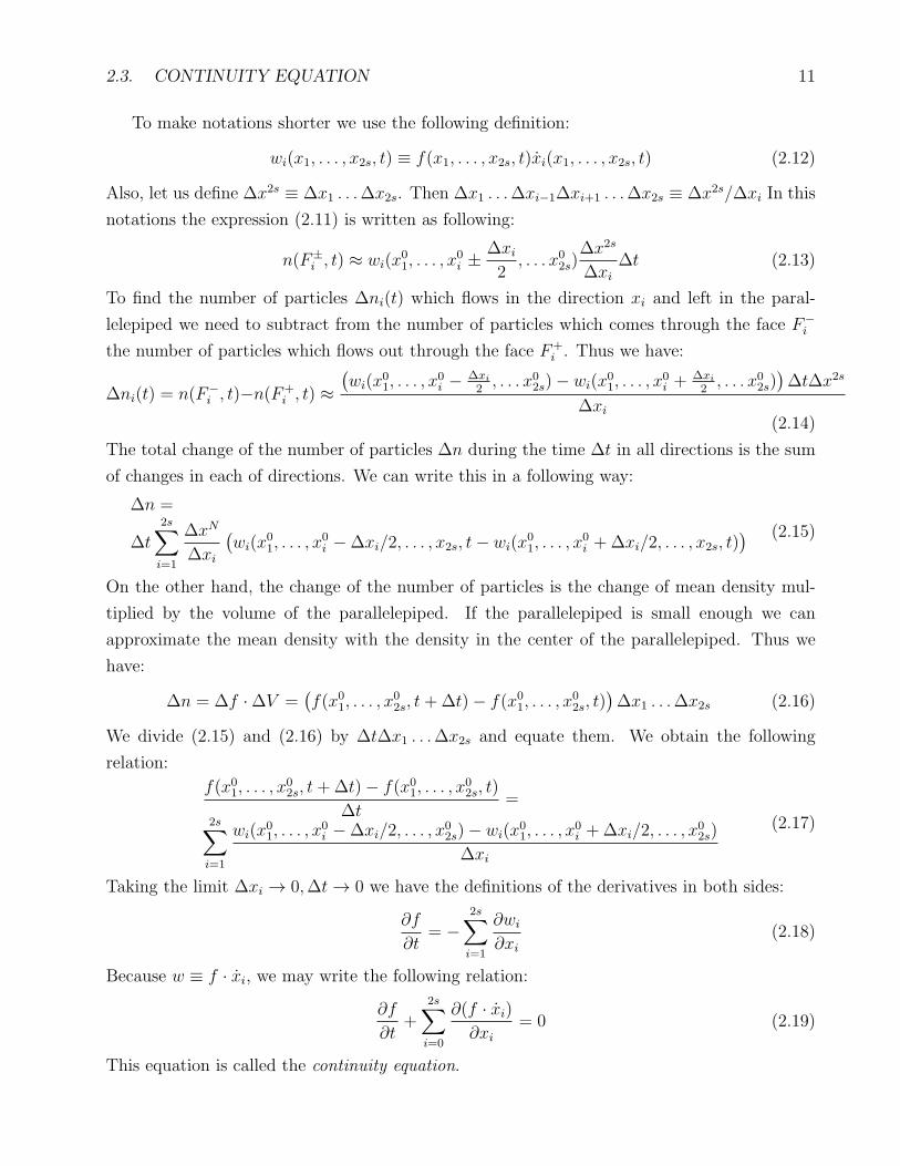
2.3. CONTINUITY EQUATION 11
To make notations shorter we use the following definition:
wi(x1, . . . , x2s, t) ≡ f(x1, . . . , x2s, t)xi(x1, . . . , x2s, t) (2.12)
Also, let us define ∆x2s ≡ ∆x1 . . .∆x2s. Then ∆x1 . . .∆xi−1∆xi+1 . . .∆x2s ≡ ∆x2s/∆xi In this
notations the expression (2.11) is written as following:
n(F±i , t) ≈ wi(x
01, . . . , x
0i ±
∆xi
2, . . . x0
2s)∆x2s
∆xi
∆t (2.13)
To find the number of particles ∆ni(t) which flows in the direction xi and left in the paral-
lelepiped we need to subtract from the number of particles which comes through the face F−i
the number of particles which flows out through the face F+i . Thus we have:
∆ni(t) = n(F−i , t)−n(F+
i , t) ≈(wi(x
01, . . . , x
0i − ∆xi
2, . . . x0
2s)− wi(x01, . . . , x
0i +
∆xi
2, . . . x0
2s))∆t∆x2s
∆xi
(2.14)
The total change of the number of particles ∆n during the time ∆t in all directions is the sum
of changes in each of directions. We can write this in a following way:
∆n =
∆t
2s∑
i=1
∆xN
∆xi
(wi(x
01, . . . , x
0i −∆xi/2, . . . , x2s, t− wi(x
01, . . . , x
0i +∆xi/2, . . . , x2s, t)
) (2.15)
On the other hand, the change of the number of particles is the change of mean density mul-
tiplied by the volume of the parallelepiped. If the parallelepiped is small enough we can
approximate the mean density with the density in the center of the parallelepiped. Thus we
have:
∆n = ∆f ·∆V =(f(x0
1, . . . , x02s, t+∆t)− f(x0
1, . . . , x02s, t)
)∆x1 . . .∆x2s (2.16)
We divide (2.15) and (2.16) by ∆t∆x1 . . .∆x2s and equate them. We obtain the following
relation:
f(x01, . . . , x
02s, t+∆t)− f(x0
1, . . . , x02s, t)
∆t=
2s∑
i=1
wi(x01, . . . , x
0i −∆xi/2, . . . , x
02s)− wi(x
01, . . . , x
0i +∆xi/2, . . . , x
02s)
∆xi
(2.17)
Taking the limit ∆xi → 0,∆t → 0 we have the definitions of the derivatives in both sides:
∂f
∂t= −
2s∑
i=1
∂wi
∂xi
(2.18)
Because w ≡ f · xi, we may write the following relation:
∂f
∂t+
2s∑
i=0
∂(f · xi)
∂xi
= 0 (2.19)
This equation is called the continuity equation.

12 CHAPTER 2. STATISTICAL MECHANICAL BACKGROUND
2.4 Liouville equation
Using the formulae (2.6) we can write the continuity equation (2.19) in the phase coordinates
pi, qi. In that case, the continuity equation (2.19) is written as
∂f
∂t+
s∑
i=1
(∂(f · qi)
∂qi+
∂(f · pi)∂pi
)
= 0 (2.20)
Opening the brackets in derivatives, we have
∂f
∂t+
s∑
i=1
(∂f
∂qiqi +
∂f
∂pipi
)
+s∑
i=1
f ·(∂qi∂qi
+∂pi∂pi
)
= 0 (2.21)
From the Hamiltonian equations (2.1) we have:
∂pi∂pi
= − ∂2H∂qi∂pi
∂qi∂qi
=∂2H∂pi∂qi
This means, that second sum in (2.21) is canceled, and equation reads as:
∂f
∂t+
s∑
i=1
(∂f
∂qiqi +
∂f
∂pipi
)
= 0 (2.22)
One can also notice that the left hand side of equation (2.22) is the full derivative of the phase
density f . Thus, the equation can be rewritten in a more compact way:
df
dt= 0 (2.23)
There is an important corollary of the Liouville equation (2.23). Let us consider a closed
system in the equilibrium state. This means that the distribution function f of this system
does not explicitly depend on time:
f(p1, . . . , ps, q1, . . . , qs, t) ≡ f(p1, . . . , ps, q1, . . . , qs) (2.24)
By integrating the Liouville equation (2.23) we have:
t1∫
t0
df
dtdt = f(p1(t1), . . . , ps(t1), q1(t1), . . . , qs(t1))− f(p1(t0), . . . , ps(t0), q1(t0), . . . , qs(t0)) = 0
(2.25)
Under considerations of the statistical mechanics the probability to find the system in certain
state does not depend on the initial configuration. Thus relation (2.25) means that distribution
function is a constant of motion of the system:
f(p1, . . . , ps, q1, . . . , qs) = f0 = const (2.26)
2.5. GIBBS DISTRIBUTION 13
And this in turn means that all the states of the system are equiprobable. Although the above
conclusions were obtained for the microcanonical ensemble where the energy conservation and
Hamiltonian equations (2.1) hold the same in principle could be true for some other systems as
well. Let in the system itself the energy conservation law does not hold. As it was mentioned
above due to the uncertainty principle the finite system can have only finite number of distin-
guishable states and thus only the finite number of different energies. Let ǫ1, ǫ2, ..., ǫm be all the
possible energies of the system. Let Ai be the set of all possible states with the energy ǫi. We
will call these sets energy levels of the system. One of the basic assumptions of the statistical
physics is that the probability to find the particle in certain state does not depend on the initial
state and on the particular trajectories of the particles. Thus, we can assume that the system
stays at each energy level for relatively long time. In that time the energy of the system is
constant and thus there exists such Hamiltonian H that satisfies Hamiltonian equations (2.1),
and thus all the states with the same energy level are equiprobable and the probability to find
the system in a certain state depends only on the energy of this state.
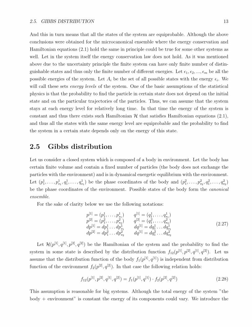
2.5 Gibbs distribution
Let us consider a closed system which is composed of a body in environment. Let the body has
certain finite volume and contain a fixed number of particles (the body does not exchange the
particles with the environment) and is in dynamical energetic equilibrium with the environment.
Let (p11, . . . , p1s1, q11, . . . , q
1s1) be the phase coordinates of the body and (p21, . . . , p
2s2, q21, . . . , q
2s2)
be the phase coordinates of the environment. Possible states of the body form the canonical
ensemble.
For the sake of clarity below we use the following notations:
p[1] = (p11, . . . , p1s1) q[1] = (q11, . . . , q
1s1)
p[2] = (p21, . . . , p2s2) q[2] = (q21, . . . , q
2s2)
dp[1] = dp11 . . . dp1s1
dq[1] = dq11 . . . dq1s1
dp[2] = dp21 . . . dp2s2
dq[1] = dq21 . . . dq2s2
(2.27)
Let H(p[1], q[1], p[2], q[2]) be the Hamiltonian of the system and the probability to find the
system in some state is described by the distribution function f12(p[1], p[2], q[1], q[2]). Let us
assume that the distribution function of the body f1(p[1], q[1]) is independent from distribution
function of the environment f2(p[2], q[2]). In that case the following relation holds:
f12(p[1], p[2], q[1], q[2]) = f1(p
[1], q[1]) · f2(p[2], q[2]) (2.28)
This assumption is reasonable for big systems. Although the total energy of the system ”the
body + environment” is constant the energy of its components could vary. We introduce the
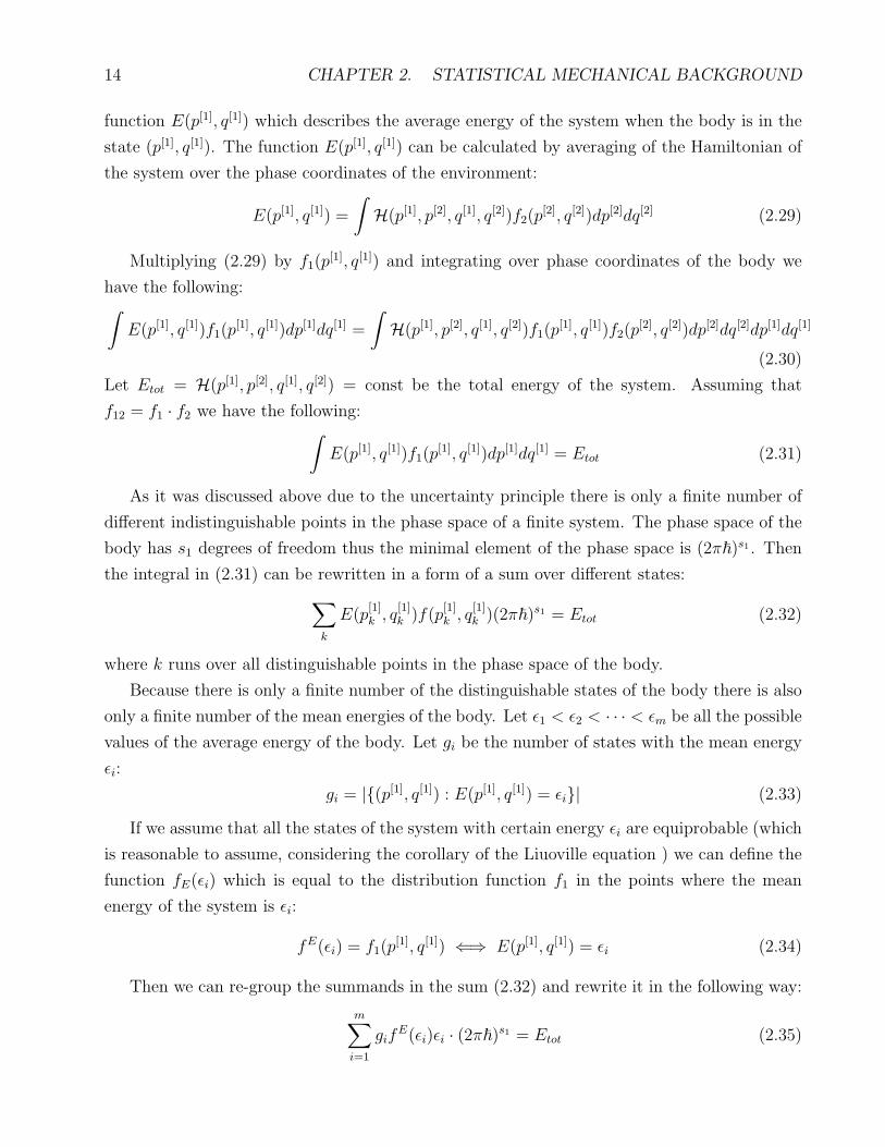
14 CHAPTER 2. STATISTICAL MECHANICAL BACKGROUND
function E(p[1], q[1]) which describes the average energy of the system when the body is in the
state (p[1], q[1]). The function E(p[1], q[1]) can be calculated by averaging of the Hamiltonian of
the system over the phase coordinates of the environment:
E(p[1], q[1]) =
∫
H(p[1], p[2], q[1], q[2])f2(p[2], q[2])dp[2]dq[2] (2.29)
Multiplying (2.29) by f1(p[1], q[1]) and integrating over phase coordinates of the body we
have the following:∫
E(p[1], q[1])f1(p[1], q[1])dp[1]dq[1] =
∫
H(p[1], p[2], q[1], q[2])f1(p[1], q[1])f2(p
[2], q[2])dp[2]dq[2]dp[1]dq[1]
(2.30)
Let Etot = H(p[1], p[2], q[1], q[2]) = const be the total energy of the system. Assuming that
f12 = f1 · f2 we have the following:∫
E(p[1], q[1])f1(p[1], q[1])dp[1]dq[1] = Etot (2.31)
As it was discussed above due to the uncertainty principle there is only a finite number of
different indistinguishable points in the phase space of a finite system. The phase space of the
body has s1 degrees of freedom thus the minimal element of the phase space is (2π~)s1 . Then
the integral in (2.31) can be rewritten in a form of a sum over different states:
∑
k
E(p[1]k , q
[1]k )f(p
[1]k , q
[1]k )(2π~)s1 = Etot (2.32)
where k runs over all distinguishable points in the phase space of the body.
Because there is only a finite number of the distinguishable states of the body there is also
only a finite number of the mean energies of the body. Let ǫ1 < ǫ2 < · · · < ǫm be all the possible
values of the average energy of the body. Let gi be the number of states with the mean energy
ǫi:
gi = |(p[1], q[1]) : E(p[1], q[1]) = ǫi| (2.33)
If we assume that all the states of the system with certain energy ǫi are equiprobable (which
is reasonable to assume, considering the corollary of the Liuoville equation ) we can define the
function fE(ǫi) which is equal to the distribution function f1 in the points where the mean
energy of the system is ǫi:
fE(ǫi) = f1(p[1], q[1]) ⇐⇒ E(p[1], q[1]) = ǫi (2.34)
Then we can re-group the summands in the sum (2.32) and rewrite it in the following way:
m∑
i=1
gifE(ǫi)ǫi · (2π~)s1 = Etot (2.35)

2.5. GIBBS DISTRIBUTION 15
Let us consider the system at some moments t1, t2, . . . , tN such that the distribution func-
tions at these moments are independent of each other. Let ni be the number of moments when
the mean energy of the system is ǫi:
ni = |tk : E(p[1](tk), q[1](tk)) = ǫi| (2.36)
Obviously the sum of ni is N :
m∑
i=1
ni = N (2.37)
If the number of moments N is large enough, then ni is proportional to the probability P (ǫi)
to find the body in the state with the mean energy ǫi:
P (ǫi) ≈ni
N(2.38)
The distribution function fE for the states with certain energy ǫi can be found using the
following formula:
fE(ǫi) · (2π~)s1 =P (ǫi)
gi(2.39)
where gi is defined by (2.33) and (2π~)s1 is an elementary element of the phase space of the body
which corresponds to one state. Putting (2.39) to the (2.35) we have the following relation:
m∑
i=1
P (ǫi)ǫi = Etot (2.40)
Using (2.38) we have the following constraint for ni:
m∑
i=1
niǫi = N · Etot (2.41)
Let us consider that n1, . . . , nm are given. Let us now count the number W of ways to
choose different states of the system at the moments t1, . . . , tN such that there will be n1 states
with the energy ǫ1, n2 states with the energy ǫ2 etc. To do it let us count the number of ways
to choose ni states at each energy level. As it was defined above, there are gi states in the
system which give the energy ǫi. We need to choose ni of them. Because the system can in
principle in two moments come to the same state, there are in total gni
i variants to do such
choice. However, if we are interested only in the number of the states but not distinguish the
order, we need to divide the total number of ways by the number of possible permutations of ni
objects, which is ni!. Thus the total number Wi of ways to choose ni states from gi possibilities
not regarding the order of chosen states is gni
i /ni!:
Wi =gni
i
ni!(2.42)
16 CHAPTER 2. STATISTICAL MECHANICAL BACKGROUND
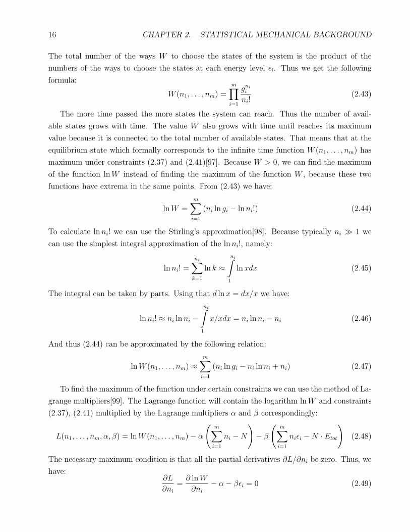
The total number of the ways W to choose the states of the system is the product of the
numbers of the ways to choose the states at each energy level ǫi. Thus we get the following
formula:
W (n1, . . . , nm) =m∏
i=1
gni
i
ni!(2.43)
The more time passed the more states the system can reach. Thus the number of avail-
able states grows with time. The value W also grows with time until reaches its maximum
value because it is connected to the total number of available states. That means that at the
equilibrium state which formally corresponds to the infinite time function W (n1, . . . , nm) has
maximum under constraints (2.37) and (2.41)[97]. Because W > 0, we can find the maximum
of the function lnW instead of finding the maximum of the function W , because these two
functions have extrema in the same points. From (2.43) we have:
lnW =m∑
i=1
(ni ln gi − lnni!) (2.44)
To calculate lnni! we can use the Stirling’s approximation[98]. Because typically ni ≫ 1 we
can use the simplest integral approximation of the lnni!, namely:
lnni! =
ni∑
k=1
ln k ≈ni∫
1
ln xdx (2.45)
The integral can be taken by parts. Using that d ln x = dx/x we have:
lnni! ≈ ni lnni −ni∫
1
x/xdx = ni lnni − ni (2.46)
And thus (2.44) can be approximated by the following relation:
lnW (n1, . . . , nm) ≈m∑
i=1
(ni ln gi − ni lnni + ni) (2.47)
To find the maximum of the function under certain constraints we can use the method of La-
grange multipliers[99]. The Lagrange function will contain the logarithm lnW and constraints
(2.37), (2.41) multiplied by the Lagrange multipliers α and β correspondingly:
L(n1, . . . , nm, α, β) = lnW (n1, . . . , nm)− α
(m∑
i=1
ni −N
)
− β
(m∑
i=1
niǫi −N · Etot
)
(2.48)
The necessary maximum condition is that all the partial derivatives ∂L/∂ni be zero. Thus, we
have:∂L
∂ni
=∂ lnW
∂ni
− α− βǫi = 0 (2.49)

2.6. ENTROPY 17
Using approximation (2.47) we get the following relation:
ln gi − lnni − 1 + 1− α− βǫi = 0 (2.50)
Now we can find the number of states ni:
ni = gie−α−βǫi (2.51)
Using the definitions of (2.38), (2.39) we can find the distribution function fE(ǫi):
fE(ǫi) =P (ǫi)
gi(2π~)s1=
ni
Ngi(2π~)s1= Ae−βǫi (2.52)
where A ≡ e−α/(N(2π~)s1). It is necessary to note, that constants A and β are the properties of
the whole system and do not depend on the current state of the system. Also, in the constraint
(2.41) Etot is the total energy of the system ”body+environment”. However, we always can
choose the zero level for the energy in such a way, that mean energy of the environment is
zero. Because the interactions between the body and environment are weak and we assume
that the distribution functions of the body and environment are independent from each other,
we may neglect the contribution to the total energy from the interactions between the particles
of body and environment. In that case the relation (2.52) signifies that the probability to find
the body in the state (p[1], q[1]) is exponentially proportional to the mean energy of this state.
The probability distribution of kind (2.52) is called Gibbs distribution.
2.6 Entropy
From the above considerations we see that the number of accessible states of the system plays
an important role in statistical mechanics. Let us consider the microcanonical ensemble with
the constant energy. Let QS be the number of states in the system. QS is a multiplicative value.
Indeed, let we have a complex system which is composed of two independent subsystems. Let
QS1 and QS
2 be the numbers of accessible states in each of subsystems correspondingly. Then
for each of QS1 states of the first system one can choose any of QS
2 states of the second systems.
The total number of states in the system is the product of numbers of states in its subsystems:
QS = QS1 ·QS
2 (2.53)
However, in practice it is more convenient to have some additive quantity which is directly
connected to QS. Such a quantity is lnQS. Thus, for the microcanonical ensemble we define
the entropy of the system in a following way:
S = kB lnQS (2.54)

18 CHAPTER 2. STATISTICAL MECHANICAL BACKGROUND
where QS is the number of accessible states in the microcanonical ensemble, kB ≈ 1.3806503 ·10−23J/K is the Boltzmann constant which is introduced due to the historical reasons and is a
coefficient in proportionality between energy and temperature. In the microcanonical ensemble
the Liouville equation (2.23) holds and all the states are equiprobable. Let f(p1, . . . , ps, q1, . . . , qs) ≡fE(E0) is the distribution function of the system, where E0 is the energy of the system. Let us
write the normalization condition for the function f :
∫
f(p1, . . . , ps, q1, . . . , qs)dp1 . . . dpsdq1 . . . dqs = 1 (2.55)
Using the discreteness of the phase space and considering that the distribution function is
constant we have the following:
QS
∑
j=1
(2π~)sfE(E0) = QS(2π~)sfE(E0) = 1 (2.56)
And so we have the relation for the number of states in the system:
QS =1
(2π~)sfE(E0)(2.57)
Putting this to (2.54) we have the following relation for the entropy:
S = −kB ln((2π~)sfE(E0)
)(2.58)
For the systems with non-constant total energy the entropy is defined by statistical averaging
the entropies of different energy levels. Thus in the canonical ensemble we have the following
definition for the entropy
S = −kB
m∑
i=1
P (ǫi) ln((2π~)sfE(ǫi)
)(2.59)
where ǫ1 < · · · < ǫm are the energy levels of the body, P (ǫi) is the probability to find the body
at the energy level ǫi, fE(ǫi) = P (ǫi)/gi where gi is the number of states on the energy level
ǫi. Considering that in canonical ensemble the distribution function fE(ǫi) follows the Gibbs
distribution (2.52) we have the following expression:
S = −kB
m∑
i=1
P (ǫi) (ln ((2π~)sA)− βǫi) (2.60)
Using the relation (2.41) and the normalizing rule∑
i P (ǫi) = 1 we get the following:
S = −kB(ln ((2π~)sA)− βE
)(2.61)
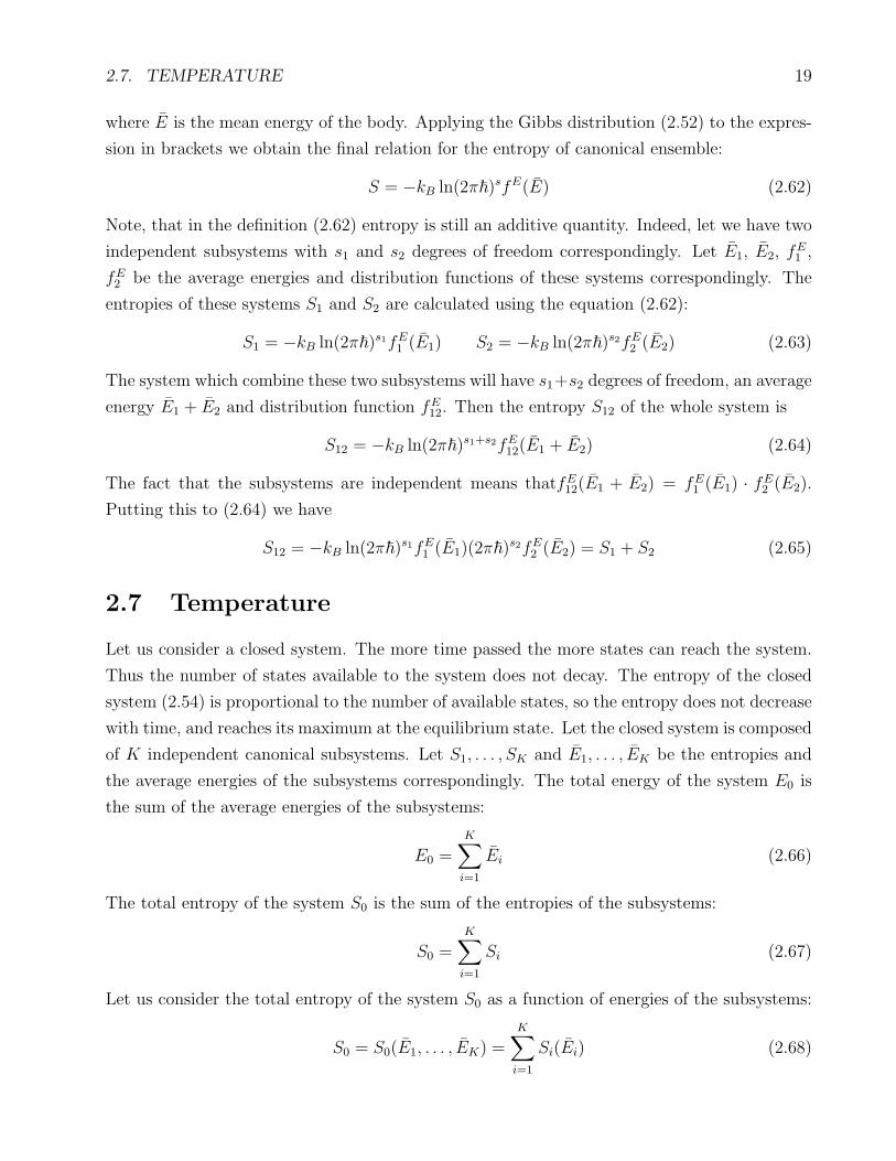
2.7. TEMPERATURE 19
where E is the mean energy of the body. Applying the Gibbs distribution (2.52) to the expres-
sion in brackets we obtain the final relation for the entropy of canonical ensemble:
S = −kB ln(2π~)sfE(E) (2.62)
Note, that in the definition (2.62) entropy is still an additive quantity. Indeed, let we have two
independent subsystems with s1 and s2 degrees of freedom correspondingly. Let E1, E2, fE1 ,
fE2 be the average energies and distribution functions of these systems correspondingly. The
entropies of these systems S1 and S2 are calculated using the equation (2.62):
S1 = −kB ln(2π~)s1fE1 (E1) S2 = −kB ln(2π~)s2fE
2 (E2) (2.63)
The system which combine these two subsystems will have s1+s2 degrees of freedom, an average
energy E1 + E2 and distribution function fE12. Then the entropy S12 of the whole system is
S12 = −kB ln(2π~)s1+s2fE12(E1 + E2) (2.64)
The fact that the subsystems are independent means thatfE12(E1 + E2) = fE
1 (E1) · fE2 (E2).
Putting this to (2.64) we have
S12 = −kB ln(2π~)s1fE1 (E1)(2π~)
s2fE2 (E2) = S1 + S2 (2.65)
2.7 Temperature
Let us consider a closed system. The more time passed the more states can reach the system.
Thus the number of states available to the system does not decay. The entropy of the closed
system (2.54) is proportional to the number of available states, so the entropy does not decrease
with time, and reaches its maximum at the equilibrium state. Let the closed system is composed
of K independent canonical subsystems. Let S1, . . . , SK and E1, . . . , EK be the entropies and
the average energies of the subsystems correspondingly. The total energy of the system E0 is
the sum of the average energies of the subsystems:
E0 =K∑
i=1
Ei (2.66)
The total entropy of the system S0 is the sum of the entropies of the subsystems:
S0 =K∑
i=1
Si (2.67)
Let us consider the total entropy of the system S0 as a function of energies of the subsystems:
S0 = S0(E1, . . . , EK) =K∑
i=1
Si(Ei) (2.68)

20 CHAPTER 2. STATISTICAL MECHANICAL BACKGROUND
At the equilibrium state the entropy of the system S0(E1, . . . , EK) has a local maximum pro-
vided that the constraint (2.66) holds. We use the Lagrange’s multipliers method and write
the Lagrange function for the entropy S0[95]:
L(Ei, . . . , EK , γ) =K∑
i=1
Si(Ei)− γ
(K∑
i=1
Ei − E0
)
(2.69)
The necessary extremum condition is equality of all the partial derivatives ∂L/∂Ei to zero.
This leads us to following equations:
∂L
∂Ei
=∂Si
∂Ei
− γ = 0 i = 1, . . . , K (2.70)
Because the entropy Si(Ei) depends only on one energy Ei the partial derivatives ∂Si/∂Ei can
be replaced with the full derivatives dSi/dEi. From (2.70) it follows that for any 1 ≤ i, j ≤ K
it holds the following:dSi
dEi
=dSj
dEj
= γ = const (2.71)
Let us introduce the value T = 1/γ which we call the temperature of the system. Note, that
for the system in the equilibrium state the temperature of all its subsystems is constant. So,
in the canonical ensemble in the equilibrium three values remain constant: number of particles
N , volume V and temperature T . That’s why the canonical ensembles are often referenced as
NVT ensembles. Now we can determine the unknown coefficients A, β in the Gibbs distribution
(2.52). Using the entropy representation (2.61) for the entropies Si we have the following:
Si = −kB(ln ((2π~)siAi)− βiEi) (2.72)
where Ai, βi are unknown Lagrange multipliers. Putting (2.72) to (2.71) we have:
dSi
dEi
= kBβi = γ =1
T= const (2.73)
So, for any 1 < i, j < K it holds βi = 1/(kBT ) = βj ≡ β.
Now we can also calculate the coefficient A in the Gibbs distribution (2.52). To do this we
can use the normalization condition for the density distribution. Putting the Gibbs distribution
(2.52) to the normalization condition (2.2) we have the following relation:
A
∫
e−βE(p1,...,ps,q1,...,qs)dp1 . . . dpsdq1 . . . dqs = 1 (2.74)
where β = (kBT )−1. Let us introduce the partition function of the system, which is defined in
a following way:
ZN = (2π~)−s
∫
e−βE(p1,...,ps,q1,...,qs)dp1 . . . dpsdq1 . . . dqs (2.75)
2.8. FREE ENERGY 21
Thus the Gibbs distribution (2.52) for the canonical ensemble read as following:
f(p1, . . . , ps, q1, . . . , qs) =1
(2π~)sZN
e−βE(p1,...,ps,q1,...,qs) (2.76)
2.8 Free Energy
Let us try to determine the physical meaning of the partition function ZN and coefficient A
in the Gibbs distribution (2.52). Let us write the definition of entropy of the system (2.62)
considering the Gibbs distribution (2.52). We obtain the following:
S = −kB ln
(1
ZN
e−βE
)
= kB lnZN +kBkBT
E (2.77)
Multiplying both parts by the temperature T and rearranging the summand we come to the
following relation:
− kBT lnZN = E − TS (2.78)
The quantity −kBT lnZN is called Helmholtz free energy of the system. We will denote it by
the symbol F :
F = −kBT lnZN = E − TS (2.79)
Let’s determine the thermodynamical sense of the Helmholtz free energy. In the thermo-
dynamics the energy which the body receives via the thermal interaction is called heat and is
denoted by Q. The first principle of thermodynamics which follows from the energy conserva-
tion law states that the sum of the change of internal energy and the work performed by the
body is equal to the heat transfered to the body:
dQ = dE + dW (2.80)
where W is the work performed by the body. Typically we assume that the work of the body is
a mechanical work performed due to changing of the volume of the body. As it is known from
mechanics, the work is a scalar product of the force by the displacement, and the force in turn
is a product of the pressure by the surface area. In the equilibrium state the average pressure
P is constant at each point and the pressure itself varies very little around the average value.
Let the surface area of the reservoir which contain the body is A. Let after performing of the
work dW each infinitesimal part of surface area dAi moved by the distance dri in the direction
perpendicular to the surface element dAi. The force which acts on the surface element dAi is
P dAi and the work to move this element is dWi = P dAidri. The value dAidri is an elementary
change of volume dVi. Thus dWi = P dVi. The total work dW can be found as the sum of
elementary works:
dW =∑
P dVi = P dV (2.81)
22 CHAPTER 2. STATISTICAL MECHANICAL BACKGROUND
In the canonical ensemble the volume is fixed thus dV = 0 and mechanical work is not per-
formed: dW = 0. Then from (2.80) we have dQ = dE. Considering (2.73) we can conclude
that the whole heat in canonical ensemble is transfered to the entropy:
dQ = dE = TdS (2.82)
Let us consider two phase process. At the first phase the body receives some heat dQ but
the volume of body is constant. In that case the energy change dE1 increases the entropy of
the body dQ = dE1 = TdS. At the second phase the body does not receive heat, but increase
its volume by dV . According to (2.80) we have 0 = dE2+PdV where dE2 is the energy change
at second phase. The total energy change of the process dE is the sum of total energies of the
pases:
dE = dE1 + dE2 = TdS − PdV = TdS − dW (2.83)
Rearranging the summands and using the definition (2.79) we can conclude that the work
performed by the body is equal to the decrease of the Helmholtz free energy dF :
dW = −(dE − TdS) = −dF (2.84)
So Helmholtz free energy shows an ability of the body to perform a work in the isothermal
process. It is necessary to notice that Helmholtz free energy should not be used for processes
where the volume is not constant. Relation (2.84) only shows that amount of the energy
received during the heat transfer in canonical ensemble in principle can be released in some
other process. To describe a processes where the volume of the system we can use the Gibbs
free energy which includes the term PV which reflects the mechanical work potential. The
definition of the Gibbs free energy G is written in a following way:
G = F + PV = H − TS = E + PV − TS (2.85)
where H is enthalpy of the system.
The change of the free energy shows whether the process is probable or not. If free energy
decreases then the energy is released during the process, so this process is spontaneous. So,
free energy can be used to determine the most probable state of the system.
2.9 Grand Canonical Ensemble
Before we considered only the systems which have a fixed number of particles. However, in the
physical chemistry it is often necessary to describe the processes where the concentrations of
substances may change. Such processes are for example diffusion and chemical reactions.

2.9. GRAND CANONICAL ENSEMBLE 23
Let us consider the system which containsm substances with changeable concentrations. Let
Ni, i = 1 . . . ,m be the quantity of the particles of ith type introduced to the system. The average
energy of the system E depends on the number of the introduced particles: E = E(N1, . . . , Nm).
Let µi, i = 1 . . . m be the energy change after introducing of one particle of ith type to the system.
Formally we can write the following relation:
µi =∂E(N1, . . . , Nm)
∂Ni
(2.86)
where E is the average energy of the system and partial derivative means the energy change after
the minimal possible change of the number of particles. The value µi is called the chemical po-
tential of the particles of ith type in the given system. Strictly speaking chemical potential of the
particle depends on the concentrations of the substances in the system, i.e µi = µi(N1, . . . , Nm).
However if the numbers of introduced particles N1, . . . , Nm are small with respect to the total
number of particles in the system the concentrations will not essentially change and thus the
chemical potentials µ1, . . . , µm can be assumed to be constant.
Let us consider the system at a fixed temperature T in a fixed volume V with fixed chemical
potentials of particles µ1, . . . , µm. Considering that for the fixed number of particles dE = TdS
the full differential of the energy can be written in a following way:
dE = TdS +m∑
i=1
µidNi (2.87)
By rearranging the summands and dividing by T we obtain the following relation for dS:
dS =dE
T−
m∑
i=1
µi
TdNi (2.88)
IfNi, i = 1, . . . ,m are small, we can assume that the entropy is linear with respect toN1, . . . , Nm.
From (2.77) it follows that the entropy is also linear with respect to the energy.
So, considering the coefficients in (2.88) we can write the following relation for the entropy:
S(N1, . . . , Nm) =1
T
(
−Ω + E −m∑
i=1
Niµi
)
(2.89)
where Ω is some constant called Grand potential. From (2.89) immediately follows the definition
of the grand potential:
Ω = E − TS −m∑
i=1
µiNi (2.90)
Let us find the probability density fG(E,N1, . . . , Nm) to find the system is in some state
(p1, . . . , ps, q1, . . . , qs) given that the average energy of this state is E and the numbers of

24 CHAPTER 2. STATISTICAL MECHANICAL BACKGROUND
introduced particles of types 1 . . . m are N1, . . . , Nm. The definition of fG given above can be
written rigorously in a following way:
fG(E0, N1, . . . , Nm) = f(p1, . . . , ps, q1, . . . , qs) ⇐⇒ s = s0+m∑
i=1
Nisi, E(p1, . . . , ps, q1, . . . , qs) = E0
(2.91)
where s0 is the number of degrees of freedom in the system without any introduced particles,
si is the number of degrees of freedom of the particle of ith type, E(p1, . . . , ps, q1, . . . , qs) is the
average energy of the system in certain state defined by (2.29). Using the relation (2.62) we
can find the entropy for any given number of introduced particles N1, . . . , Nm:
S(N1, . . . , Nm) = −kB ln(2π~)s0+∑
NisifG(E,N1, . . . , Nm) (2.92)
Putting this to (2.89) we have the following:
− kB ln(2π~)s0+∑
NisifG(E,N1, . . . , Nm) =1
T
(
−Ω + E −m∑
i=1
µiNi
)
(2.93)
From this relation we can find fG:
fG(E,N1, . . . , Nm) =1
(2π~)s0+∑
NisieβΩe−βE+
∑
βµiNi (2.94)
The grand partition function Ω can be found from the normalization rule for fG. The total
probability to find the system in some state with some number of particles N1, . . . , Nm is unity.
Thus, considering (2.94) we can write the following normalization:
eβΩ ·∑
N1,...,Nm
λN11 . . . λNm
m
(2π~)s0+∑
Nisi
∫
e−βE(p1,...,ps,q1,...,qs)dp1 . . . dpsdq1 . . . dqs = 1 (2.95)
where sum is taken over all possible values of N1, . . . , Nm, λi ≡ eµi is activity of the ith type of
particles. The grand potential can be written in a following form:
Ω = kBT ln1
Ξ= −kBT ln Ξ (2.96)
where Ξ =∑
N1,...NmλN11 . . . λNm
m ZN1,...,Nmis the Grand partition function, ZN1,...,Nm
is the canon-
ical partition function for particular values N1, . . . , Nm.
2.10 Solubility and Solvation Free energy
The solubility in water and other fluids in the human body is one of the important proper-
ties of drugs and drug-like compounds used in medicine, because it shows the drug ability

2.10. SOLUBILITY AND SOLVATION FREE ENERGY 25
to be delivered to the place there it works. Free energy is the energetic characteristic of the
chemical system which allow to describe and predict many chemical processes including the
dissolution process. The dissolution process by itself can be divided into two phases: 1) De-
stroying the crystal structure, transition from the crystal to the “free” state. 2) Solvatation of
the molecule. The energy of the transition from the crystal to the “free” state can be with a
reasonable accuracy estimated with quantum-mechanical methods[7]. The second phase (sol-
vation of the molecule) is energetically described by the solvation free energy (SFE). SFE is
the free energy change during the transfer of the compound from the free (gas) phase to a solu-
tion. Although SFE can be measured experimentally, these experiments are quite complicated
from the technical point of view especially for compounds with low solubility and low volatility
[65]. Computation of the SFE is also a challenging task, because solvation process involves a
many-body interactions of the solvent molecules. Typically calculation of the SFE with the
molecular dynamics or Monte Carlo simulations may take several days or even weeks, and will
not necessarily be accurate enough. In our work we use much faster method which is based on
the classical density functional theory and integral equation theory of liquids.

Chapter 3
Integral Equation Theory of Liquids.
RISM and 3DRISM
In this chapter the basics of the classical density functional theory and the reference interac-
tion site model (RISM) are described. The chapter contains definitions of the distribution and
correlation functions, free-energy functional methods, derivation of Ornstein-Zernike,RISM and
3DRISM equations and closure relations. Theoretical questions which are necessary for numer-
ical solution of RISM equations are discussed. The chapter is mostly based on Refs. [50], [95]
and [24]. Some derivations are adopted for the six-dimensional case and multi-particle systems.
Many technicalities can be found in the specialized mathematical literature.
3.1 System under investigation
We did not make any assumptions about the particles in the systems which we described.
We only assume that there are many particles in the system, and that the motion of the
particles is quasi-chaotic. We define the macroscopic parameters of the system, such as Entropy,
Temperature and Free energy and relate them to each other. This allows us to predict the state
of the system and the energy changes in the thermodynamic processes. Integral equation theory
of liquids (IETL) allows to predict some specific microscopic and macroscopic thermodynamic
parameters of fluids, i.e. the local solvent structure around the solute, free energy of solvation
etc.
The simplest model of fluid is the system composed of the spherical particles which interact
via pairwise additive potential. This model allows us to describe noble gases, electrolyte solu-
tions and other systems where the shape of the particles does not affect much the properties of
the fluid. However, properties of many physical chemical systems of interest essentially depend
on the shape of the molecules and partial charges of the atoms of the molecules. For those
systems the model of spherical particles is unable to give reliable results. That’s why we will
26

3.2. CONFIGURATIONAL INTEGRAL 27
use the model which accounts the shape of the molecules. The molecules in our model are
described as the rigid objects, which means that the distances of the atoms in the molecule
are fixed. Position of the rigid molecule can be described by three coordinates of the center of
mass r = (x, y, z) and three Euler angles θ = (θx, θy, θz). Interactions between the molecules
can be described by the potential U12(r2 − r1,θ1 − θ2) where (r1,θ1) and (r2,θ2) are the
positions and rotations of the first and second molecules correspondingly. This model gives
much better description of the fluid than the spherical particles model. However, it also does
not consider many effects related to the motion of the molecules, e.g. conformational changes
of the molecules, vibrations of the atoms etc. The model gives relatively good description of
the fluids composed of the small or rigid molecules, e.g. water, carbon hydroxide, benzene etc.
This model is not ideal by any means, however it can give insights to many important systems
in physical chemistry. The reason why we use this model is that more detailed models with
non-rigid molecules often appear to be too complicated to be simulated from the computational
point of view.
3.2 Configurational integral
In many cases the general formula (2.79) is not suitable for practical free energy calculations
due to unknown partition function (2.75). However there are some systems for which the
partition function can be calculated easily. One of such systems is the ideal gas. For non-
ideal gas systems one can separate the ideal and non-ideal contributions to the free energy
which also can simplify the calculations. Let us now consider the general case of the system
of N interacting rigid particles. Total energy of the system can be represented as a sum of
kinetic energy term K and potential energy term U , where kinetic energy depends only on
the generalized momenta of the system and the potential energy depends only on generalized
coordinates of the system. Let us consider the canonical ensemble which contains N molecules.
We consider that the molecules are rigid. Then the potential energy U depends on positions
r1, . . . , rN and orientations θ1, . . . ,θN : U = U(r1, . . . , rN,θ1, . . . ,θN ). From the mechanics it
is known that the motion of the rigid body can be described by the movement of its center
of mass and rotation of the body around the perpendicular axes which come through the
center of mass of the body[96]. Let pk = (pkx, pky, p
kz) be the linear momentum of the kth
particle, lk = (lkx, lky , l
kz ) be the angular momentum of the kth particle around the perpendicular
axes which come through the center of mass of the body. As it is known from the course of
mechanics, the kinetic energy of the body is a sum of translational and rotational kinetic energy.
Let v0(t) be the velocity of the center of mass of the molecule. At each moment of time t we
can introduce the coordinate system which is located in the center of mass of the molecule and

28 CHAPTER 3. INTEGRAL EQUATION THEORY OF LIQUIDS. RISM AND 3DRISM
moving with the speed v0(t). Let us choose at the moment t the coordinate axes of the system
in some known ”local” directions (e.g. which go through some certain atoms of the molecule).
However, let the orientation of the axes be fixed with respect to the initial system. Let there
are M different types of molecules in the system. Let ak ∈ 1, . . . ,M be the type of the kth
molecule. Let mak be the mass of the molecule of type ak. Thus, in a new coordinate system
the center of mass of the molecule is immovable, however the molecule by itself is rotating. The
kinetic energy with respect to this system differs from the kinetic energy with respect to initial
system by makv0(t)2/2. Let Jx
ak, Jy
ak, Jz
akbe the moments of inertia of the molecule of type
ak about the chosen axes. Then the rotational kinetic energy can be found by the following
relation:
Krot =(lkx)
2
2Jxak
+(lky)
2
2Jyak
+(lkz )
2
2Jzak
(3.1)
The total kinetic energy of the molecule is a sum of the rotational kinetic energy and the
translational kinetic energy of the center of mass of the molecule. It can be written in a
following way:
Kk =(pkx)
2 + (pky)2 + (pkz)
2
2mak
+(lkx)
2
2Jxak
+(lky)
2
2Jyak
+(lkz )
2
2Jzak
(3.2)
For the sake of uniformity, let us use the following definitions:
p6k−5 ≡ pkx p6k−2 ≡ lkxp6k−4 ≡ pky p6k−1 ≡ lkyp6k−3 ≡ pkz p6k ≡ lkz
(3.3)
B6k−5 ≡ B6k−4 ≡ B6k−3 ≡ mak
B6k−2 ≡ Jxak
B6k−1 ≡ Jyak
B6k ≡ Jzak
(3.4)
where k = 1 . . . N
Using the above definitions the kinetic energy of the system can be written in a following
way:
K(p1, . . . , p6N ) =6N∑
i=1
p2i2Bi
(3.5)
The total energy of the system is a sum of kinetic and potential energy components. This can
be written in a following way:
E(p1, . . . , p6N , r1, . . . , rN,θ1, . . . ,θN ) =6N∑
i=1
p2i2Bi
+ U(r1, . . . , rN,θ1, . . . ,θN ) (3.6)
where U(r1, . . . , rN,θ1, . . . ,θN ) is a potential energy of the system. Here and below saying “the
total energy of the system” we mean the total average energy of the system, where averaging
is done over the degrees of freedom of the environment as it was done in the the section 2.5.

3.2. CONFIGURATIONAL INTEGRAL 29
Let us find the partition function of the system ZN1...NMwhere N1 . . . NM are the numbers
of particles of different kind in the system. In the general definition of partition function (2.75)
the integration is performed over all distinguishable states of the system. We suppose that the
particles of each kind are indistinguishable. Then there are Nk! ways to select Nk particles of
kind k. The total number of ways to select particles of all kinds is N1! · · · · ·NM !. We need to
normalize the integral in the definition of the partition function considering this number. Then
the partition function ZN1...NMis defined in a following way:
ZN1...NM=
1
(2π~)6NN1! . . . NM !
∫
e−β
∑6Ni=1
p2i2Bi
−βU(r1,...,rN,θ1,...,θN )dp1 . . . dp6Ndr1 . . . drNdθ1 . . . dθN
(3.7)
One can notice that the integration over momenta components can be done separately:
∫
e−β
∑6Ni=1
p2i2Bi dp1 . . . dp6N =
6N∏
i=1
∞∫
−∞
e−β
p2i2Bi dpi (3.8)
To calculate contribution of each component we can use a known formula for Gaussian integral
[100]:∞∫
−∞
e−x2
dx =√π (3.9)
To prove this relation we define I =∫∞−∞ e−x2
dx. Then I2 =∫e−x2
dx∫e−y2dy =
∫ ∫e−(x2+y2)dxdy.
Switching to the polar coordinates we have x = r cosφ, y = r sinφ, dxdy = rdrdφ, I2 =∫∞0
∫ 2π
0e−r2rdrdφ = −π
∫∞0
e−r2(−2r)dr. Considering that −2rdr = d(−r2) we have I2 =
−π(e∞ − e0) = π, thus I =√π. Using this equality we can write the following:
6N∏
i=1
∞∫
−∞
e−β
p2i2Bi dpi =
6N∏
i=1
√
2BikBT
∫
e−(
pi√2BikBT
)2
dpi√2BikBT
=6N∏
i=1
√
2πBikBT (3.10)
Considering the definitions of Bi (3.4) we can return to the original masses and momenta of
inertia of the particles:
6N∏
i=1
√
2πBikBT =N∏
i=1
(2πkBT )6/2(mai)
3/2(JxaiJyaiJzai)1/2 (3.11)
Putting this to the definition of the partition function (3.7) and considering that (2π~)6N =∏
a(2π~)6Na we have the following:
ZN1...NM=
M∏
a=1
((2π~kBT )
3(m3aJ
xaJ
yaJ
za )
1/2
(2π~)6
)Na1
Na!
∫
e−βU(r1,...,rN,θ1,...,θN )dr1 . . . drNdθ1 . . . dθN
(3.12)

30 CHAPTER 3. INTEGRAL EQUATION THEORY OF LIQUIDS. RISM AND 3DRISM
We define the configurational integral QN1...NMin a following way:
QN1...NM=
∫
e−βU(r1,...,rN,θ1,...,θN )dr1 . . . drNdθ1 . . . dθN (3.13)
Then the partition function can be written in a following form:
ZN1...NM=
M∏
a=1
DNaa
Na!QN1...NM
(3.14)
where Da
√
m3aJ
xaJ
yaJz
a (kBT )3(2π)−3
~−6.
We will use the functions ZN1...NMand QN1...NM
in our work. However, we find it also
necessary to write the exact expression for the functions ZN and QN for the liquid of N
identical spherical particles. In that case there will be no integration over the angular degrees
of freedom in (3.7), and the partition function ZN is written in a following way:
ZN =1
Λ3NN !QN (3.15)
where QN =∫exp(−βU(r1, . . . , rN))dr1 . . . drN, Λ =
√
2π~2/(mkBT ) is a thermal de Broglie
wavelength, m is a mass of the particle.
3.3 Density distribution functions
Putting the expression for the average energy of the system (3.6) to the Gibbs distribution
(2.52) we obtain the following:
f(p1, . . . , p6N , r1, . . . , rN,θ1, . . . ,θN ) =6N∏
i=1
e−β
p2i2Bi
~√2πBikBT
· N1! . . . NM !
QN1...NM
e−βU(r1,...,rN,θ1,...,θN )
(3.16)
≡ fp(p1, . . . , p6N) · fq(r1, . . . , rN,θ1, . . . ,θN )
where kinetic and potential components fp, fq of the distribution function f are defined in a
following way:
fp(p1, . . . , p6N ) =6N∏
i=1
1
~√2πBikBT
e−β
p2i2Bi (3.17)
fq(r1, . . . , rN,θ1, . . . ,θN ) =N1! . . . NM !
QN1...NM
e−βU(r1,...,rN,θ1,...,θN ) (3.18)
We can see that kinetic component fp is product of the probability distributions of momenta
components. In such a way we can find the probability that the momenta degree of freedom
has a certain value pi:
f ip(pi) =
1
2π~√BikBT
e−β
p2i2Bi (3.19)

3.3. DENSITY DISTRIBUTION FUNCTIONS 31
For the distribution fq in a general case such a representation is not possible, because the
potential energy U connects the coordinates of all particles.
Speaking about the potential component, we also rarely need to know positions of all parti-
cles. It is more useful to know the mean number of particles at some selected positions, where
number of such positions is much smaller than number of particles. For the one-component
system we define the n-particle density distribution function ρ(n)(r1, . . . , rn,θ1, . . . ,θn)) in a
following way:
ρ(n)(r1, . . . , rn,θ1, . . . ,θn) =N !
(N − n)!
∫e−βU(r1,...,rN,θ1,...,θN )
QN1...NM
drn+1 . . . drNdθn+1 . . . dθN
(3.20)
The similar definition can be given for the multi-component systems as well. However, in
general case this definition is too cumbersome to be written. For the practical application the
most interesting are one-particle and two-particle density distribution functions. We define the
one-particle distribution function ρa of particles of type a in a following way:
ρa(r1,θ1) = Na
∫e−βU(r1,...,rN,θ1,...,θN )
QN1...NM
dr2 . . . drNdθ2 . . . dθN (3.21)
where it is assumed that the particle with coordinates (r1,θ1) has type a. Two-particle distri-
bution function ρab for the particles of types a, b is defined in a following way:
ρab(r1, r2,θ1,θ2) = Na(Nb − δab)
∫e−βU(r1,...,rN,θ1,...,θN )
QN1...NM
dr3 . . . drNdθ3 . . . dθN (3.22)
where δab is a Kronecker’s delta and it is assumed that the particles with the coordinates
(r1,θ1), (r2,θ2) have types a and b correspondingly.
Also, we define the dimensionless pair density correlation function gab in a following way:
gab(r1, r2,θ1,θ2) =ρab(r1, r2,θ1,θ2)
ρa(r1,θ1)ρb(r2,θ2)(3.23)
We note that considering the properties of the Dirac delta-function the definitions of the
density distribution functions (3.21), (3.22) can be written in a following form[50]:
ρa(r1,θ1) =
∫ Na∑
i=1
δ(rai − r1)δ(θai − θ1)
e−βU(r1,...,rN,θ1,...,θN )
QN1...NM
dr1 . . . drNdθ1 . . . dθN (3.24)
=
⟨Na∑
i=1
δ(rai − r1)δ(θai − θ1)
⟩
ρab(r1, r2,θ1,θ2) =
⟨Na∑
i=1
Nb∑
j=1
(1− δabδij)δ(rai − r1)δ(θ
ai − θ1)δ(r
bj − r2)δ(θ
bj − θ2)
⟩
(3.25)
32 CHAPTER 3. INTEGRAL EQUATION THEORY OF LIQUIDS. RISM AND 3DRISM
where (rai ,θai ) is the coordinates of ith particle of type a.
We should also note, that (4.3) can be simplified for the systems with pairwise additive
potential. Let the particles in the system interact via the pair-additive potential U(r[N ],θ[N ]),
which is defined in a following way:
U(r[N ],θ[N ]) =1
2
M∑
b=1
M∑
c=1
Nb∑
i=1
Nc∑
j=1
(1− δbcδij)ubc(rcj − rbi ,θ
cj − θc
i ) (3.26)
where ubc(r,θ) is the interaction potential between the particles of type b and c.
Let the potential energy linearly depends on λ. So, the functions ubc(r[N ],θ[N ];λ) are defined
in a following way:
ubc(r,θ;λ) = ubc0 (r,θ) + λ∆u(r,θ) (3.27)
where ubc0 , is the particle interaction potential in the initial system, ∆ubc = ubc
1 −ubc0 , u
bc1 (r,θ) is
particle interaction potential in the final system. In such considerations we have ∂U/∂λ = ∆U ,
where ∆U is defined in a following way:
∆U(r[N ],θ[N ]) =1
2
M∑
b=1
M∑
c=1
Nb∑
i=1
Nc∑
j=1
(1− δbcδij)∆ubc(rcj − rbi ,θcj − θc
i ) (3.28)
Putting this representation to the thermodynamical integration formula (4.3) we have the
following expression:
〈∂U/∂λ〉 =1
2
M∑
b=1
M∑
c=1
Nb∑
i=1
Nc∑
j=1
(1− δbcδij)
∫
drbidθbidr
cjdθ
cj∆ubc(rcj − rbi ,θ
cj − θc
i )
(∫
e−βU(r[N ],θ[N ] dr[N ]dθ[N ]
drbidθbidr
cjdθ
cj
)
(3.29)
Using the definition of the pair correlation function (3.22) and changing the sum over identical
particles to the product we come to the following expression for the thermodynamic integration
process:
∆F =1
2
M∑
b=1
M∑
c=1
∫
ρbc(r2 − r1,θ2 − θ1)∆ubc(r2 − r1,θ2 − θ1)dr1dr2dθ1dθ2 (3.30)
3.4 Free Energy functional
Before we consider systems with the uniform density. However, if some external field acts on
the particles of the system the density can change. Also, we can consider not necessarily the
equilibrium state of the system. In such cases it can be necessary to consider dependency of the
free energy of the system on the external factors such as external field or density distribution.

3.4. FREE ENERGY FUNCTIONAL 33
Let the system contains N1, . . . , NM particles of types 1, . . . ,M correspondingly. We denote as
(rai ,θai ) the coordinates of the i
th particle of type a. Then the external field VN can be expressed
as follows:
VN(r[N ],θ[N ]) =
M∑
a=1
Na∑
i=1
φa(rai ,θai ) (3.31)
where N =∑
aNa, r[N ] ≡ (r11, . . . , r
1N1, . . . , rM1 , . . . , rMNM
),
θ[N ] ≡ (θ11, . . . ,θ
1N1, . . . ,θM
1 , . . . ,θMNM
), φa(r,θ) is an external field which acts on the particle of
type a at position (r,θ).
Using the Gibbs distribution (2.76) together with the relation (3.16) we can write the
following:
fp(p1, . . . , p6N )fq(r[N ],θ[N ]) =
1
(2π~)6NZN1...NM
e−β
∑ p2i2Bi
−βU(r[N ],θ[N ])−βV (r[N ],θ[N ])(3.32)
Integrating both parts over the momenta components p1, . . . , p6N we get the following:
fq(r[N ],θ[N ]) =
M∏
a=1
DNaa
Na!
1
ZN1...NM
e−βU(r[N ],θ[N ])−βV (r[N ],θ[N ]) (3.33)
Form this relation we can express ZN1...NMas a function of fq in certain point (r1, . . . , rN,θ1, . . . ,θN ):
ZN1...NM(r[N ],θ[N ]) =
M∏
a=1
DNaa
Na!
e−βU(r[N ],θ[N ])−βV (r[N ],θ[N ])
fq(r[N ],θ[N ])(3.34)
Similarly to the general definition of the free energy of the system (2.79) we can define the free
energy as a function of the density in certain point:
F(r[N ],θ[N ]) = −kBT lnZN1...NM=
kBT lnM∏
a=1
Na!
DNaa
+ kBT ln fq(r1, . . . , rN,θ1, . . . ,θN ) + U(r[N ],θ[N ]) + V (r[N ],θ[N ])(3.35)
We introduce the Free energy functional as the ensemble average of the expression (3.35) over
all distinguishable points of the phase space, namely:
F [fq] =⟨F(r[N ],θ[N ])
⟩=
kBTM∑
a=1
lnNa!
DNaa
+
∫
fq(r[N ],θ[N ])
(kBT ln fq(r
[N ],θ[N ]) + U(r[N ],θ[N ]) + V (r[N ],θ[N ]))dr[N ]dθ[N ]
(3.36)
3.4.1 Minimization property of the free energy functional
One of the important properties of the free energy functional is that for the equilibrium density
f 0q = A/ZN1...NM
exp(−βU − βV ) where A =∏
aDNaa /Na! it has the minimum1.
1In this section we omit the arguments (r[N ],θ[N ]) of fq, f0q for the sake of simplicity.

34 CHAPTER 3. INTEGRAL EQUATION THEORY OF LIQUIDS. RISM AND 3DRISM
For the f 0q it holds the following:
kBT ln f 0q (r
[N ],θ[N ]) = kBT lnA/ZN1...NM− U − V (3.37)
Putting this to the definition of the free energy (3.36) we have the following:
F [f0q ] =
∫
f 0q (r
[N ],θ[N ]) (kBT lnA/ZN1...NM− U − V + U + V ) dr[N ]dθ[N ] = kBT lnA/ZN1...NM
(3.38)
Using this formula we can find the difference ∆F = F [fq]−F [f0q ]. We will have the following:
∆F =
∫
fq
(
kBT ln fq + kBT lnA
ZN1...NM
− kBT ln f 0q
)
dr[N ]dθ[N ] − kBT lnA
ZN1...NM
(3.39)
where U + V was changed to kT lnA/Z − kT ln f 0q as a result of (3.37). Considering, that due
to normalization∫fq =
∫f 0q = 1, we have the following
∆F = kBT
∫ (
fq lnfqf 0q
+ fq − f 0q
)
dr[N ]dθ[N ] = kBT
∫
f 0q
(fqf 0q
lnfqf 0q
+fqf 0q
− 1
)
dr[N ]dθ[N ]
(3.40)
The integrand is always positive. To prove it we denote fq/f0q ≡ 1/B. We have fq
f0qln fq
f0q+ fq
f0q−1 =
1/B ln 1/B + 1/B − 1 = 1/B(− lnB + 1 − B). It is known, that for any B > 0 it holds that
lnB ≤ B − 1, thus considering that fq, f0q ≥ 0 we conclude that the integrand is always
non-negative and ∆F ≥ 0.
3.5 Free energy functional of the ideal gas in an external
field
One of the basic assumptions of the density functional theory is that the free energy functional
can be expressed as a functional of one-particle densities ρ1(r1,θ1), . . . , ρM(rM ,θM ) of the
particles of types 1, . . . ,M correspondingly. In the ideal gas the particles do not interact
to each other, so the probability to find the system in certain configuration is a product of
probabilities to find one-particle at certain position. Considering the normalization of ρa(r,θ)
we can write the following:
fq(rN ,θN ) =
M∏
a=1
Na∏
i=1
ρa(rai ,θai )
Na
(3.41)
Putting this to the definition of the free energy functional (3.36) and considering that for ideal
gas in external field U = 0 we have the following:
F [ρ1, . . . ,ρM ] = S1 + S2 + S3 (3.42)

3.5. FREE ENERGY FUNCTIONAL OF THE IDEAL GAS 35
where summands S1, S2, S3 are defined in a following way
S1 =M∑
a=1
kBT lnNa!
DNaa
(3.43)
S2 = kBT
∫ M∏
b=1
Nb∏
j=1
ρb(rbj,θbj)
Nb
lnM∏
a=1
Na∏
i=1
ρa(rai ,θai )
Na
dr[N ]dθ[N ] (3.44)
S3 =
∫ M∏
b=1
Nb∏
j=1
ρb(rbj ,θbj)
Nb
M∑
a=1
Na∑
i=1
φa(rai ,θai )dr
[N ]dθ[N ] (3.45)
Using the Stirling’s approximation (2.46) we rewrite the first summand in a following way:
S1 ≈ kBT
M∑
a=1
(Na lnNa −Na −Na lnDa) = kBT
M∑
a=1
Na(lnNa
Da
− 1) (3.46)
Considering the normalization∫ρa = Na the first summand can be re-written in a following
way:
S1 ≈ kBT
M∑
a=1
∫
ρa(r,θ)
(
lnNa
Da
− 1
)
drdθ (3.47)
Considering that the logarithm of the product is the sum of logarithms we can re-write the
second summand in a following way:
S2 =M∑
a=1
Na∑
i=1
kBT
∫
drai dθai
ρa(rai ,θai )
Na
lnρa(rai ,θ
ai )
Na
∫∏
j 6=i
ρa(raj ,θaj )
Na
∏
b 6=a
Nb∏
k=1
ρb(rbk,θbk)
Nb
dr[N ]/drai dθ[N ]/dθa
i
(3.48)
where dr[N ]/drai dθ[N ]/dθa
i means integration over all coordinates except (rai ,θai ). From the
normalization∫ρa/Na = 1 we conclude that integral over dr[N ]/drai dθ
[N ]/dθai gives unity. Also,
considering that all particles of the same type are indistinguishable, we can substitute the
sum over i by the multiplication by Na. Thus we have the following expression for the second
summand:
S2 =M∑
a=1
∫
ρa(r,θ) lnρa(r,θ)
Na
drdθ (3.49)
Similarly, the third summand (3.45) can be expressed in a following way:
S3 =M∑
a=1
Na∑
i=1
∫
drai dθai
ρa(rai ,θai )
Na
φa(rai ,θai )
∫∏
j 6=i
ρa(raj ,θaj )
Na
∏
b 6=a
Nb∏
k=1
ρb(rbk,θbk)
Nb
dr[N ]/drai dθ[N ]/dθa
i
(3.50)
Considering the normalization of the ρa and changing sum over Na identical particles to mul-
tiplication we have the following expression:
S3 =Na∑
a=1
∫
ρa(r,θ)φa(r,θ)drdθ (3.51)
36 CHAPTER 3. INTEGRAL EQUATION THEORY OF LIQUIDS. RISM AND 3DRISM
Combining the expressions for S1, S2, S3 we have:
F [ρ1, . . . ,ρM ] =M∑
a=1
kBT
∫
ρa(r,θ)
(
lnNa
Da
− 1 + lnρa(r,θ)
Na
)
drdθ+Na∑
a=1
∫
ρa(r,θ)φa(r,θ)drdθ
(3.52)
Considering that the sum of logarithms is a logarithm of product we can avoid Na and write
the final expression for the free energy functional of ideal gas:
F id[ρ1, . . . ,ρM ] =M∑
a=1
kBT
∫
ρa(r,θ)
(
lnρa(r,θ)
Da
− 1
)
drdθ +M∑
a=1
∫
ρa(r,θ)φa(r,θ)drdθ
(3.53)
In the general case of non-ideal gas the free energy can be expressed as a sum of ideal and
exchange parts:
F [ρ1, . . . ,ρM ] = F id[ρ1, . . . ,ρM ] + F ex[ρ1, . . . ,ρM ] (3.54)
3.6 Functional derivatives
Let us consider a linear functional F [ρ] which maps the function ρ : R3 → R to the real space.
Let us consider the case then the functional F can be represented in a following way:
F [ρ] =
∫
R3
A[ρ](r)ρ(r)dr (3.55)
where A[ρ] : R3 → R is defined for each ρ. In that case the functional is called differentiable
and the expression A[ρ] is called functional derivative of the functional F . The functional
derivative of the functional F with respect to the function ρ in the point r is denoted in a
following way:
A[ρ](r) ≡ δFδρ(r)
(3.56)
For non-linear functionals the functional derivative can be introduced by linearization of the
functionals in some neighborhood. Let now F be a non-linear functional and there exists such
neighborhood of a function ρ0 that for any function ρ from this neighborhood the following
relation holds:
F [ρ] = F [ρ0] +
∫
R3
A[ρ0](r) (ρ(r)− ρ0(r)) dr+ o(||ρ− ρ0||) (3.57)
where || · || is some norm of the functions defined on R3. In that case the functional F is called
differentiable in the point ρ0 and A[ρ0] is called the functional derivative. We should note that
more strict and general definition of the functional derivatives can be given using the concepts
of Frechet and Gateaux derivatives. More information can be found in Ref. [101].

3.7. DIRECT CORRELATION FUNCTIONS 37
Many properties of functional derivatives can be determined using the properties of the
partial derivatives. Let us consider the case when the functional F is defined only for the
piecewise constant functions. Let additionally these piecewise constant functions have final
support V ⊂ R3. Let the set V is divided to the non-intersecting subsets V1, . . . , VN . We define
the functional F for all functions ρ(r) which have constant values on the sets Vi. We choose
the points r1, . . . , rN in such a way that ri ∈ Vi, i = 1, . . . , N . In that case expression (3.57)
can be written in a following way:
F [ρ] = F [ρ0] +N∑
i=1
δFδρ0(ri)
µ(Vi)(ρi − ρ0i
)+ o(||ρ− ρ0||) (3.58)
where µ(Vi) is the volume of the set Vi, ρi = ρ(ri), ρ0i = ρ0(ri). Using the properties of the
partial derivatives we come to the following relation:
δFδρ0(ri)
µ(Vi) =∂F∂ρ0i
(3.59)
Using this relation when N → ∞ it is possible to obtain the properties of the functional
derivatives.
For example, let us consider one of the simplest functional F [ρ] ≡ ρ(r0) where ir0 is some
given point. Our aim is to find the functional derivative δF/δρ(r) ≡ δρ(r0)/δρ(r). Let us
consider a case of piecewise constant functions. Let r0 ∈ V1, r ∈ Vi. From (3.59) we have the
following:δρ(r0)
δρ(r)µ(Vi) =
∂ρ0i∂ρi
= δ1i (3.60)
where δ1i is the Kronecker delta. Now we consider the case N → ∞, µ(Vi) → 0. We have the
following relation:δρ(r0)
δρ(r)= lim
µ(Vi)→0
δ1iµ(Vi)
= δ(r− r0) (3.61)
where δ(r− r0) is Dirac delta function.
Other properties of the functional derivatives can be obtained using the similar procedure.
The most of the properties of the partial derivatives are also valid for the functional derivatives
if one changes symbols ∂ to δ and summation to the integration over R3.
3.7 Direct correlation functions
In the density functional theory responses of the free energy functionals to the local change
of the density play an important role. To characterize this response one needs to know the
functional derivatives of the free energy functional with respect to the density. Let us find the
functional derivative of the free energy functional (3.54) with respect to the density of particles

38 CHAPTER 3. INTEGRAL EQUATION THEORY OF LIQUIDS. RISM AND 3DRISM
of type a in the point (r1,θ1). Using the properties of functional derivatives we write the
following:
δFδρa(r1,θ1)
=M∑
b=1
∫ (
kBTδρb(r,θ)
δρa(r1,θ1)ln
ρb(r,θ)
Da
+δρb(r,θ)
δρa(r1,θ1)φa(r,θ)
)
drdθ +δF ex
δρa(r1,θ1)
(3.62)
From the properties of the functional derivatives it we conclude that the following relation
holds:δρb(r,θ)
δρa(r1,θ1)= δabδ(r1 − r,θ1 − θ) (3.63)
where δ(r1−r,θ1−θ) = δ(r1−r)δ(θ1−θ) Using this relation we come to the following relation:
δFδρa(r1,θ1)
= kBT lnρa(r1,θ1)
Da
+ φa(r1,θ1) +δF ex
δρa(r1,θ1)(3.64)
We define the direct correlation function ca(r1,θ) in a following way:
ca(r1,θ) ≡ −βδF ex
δρa(r1,θ1)(3.65)
As it was proven in the section 3.4.1 the free energy functional reaches its minimum at the
equilibrium density under constrains of the density normalization which can be written as∫ρa = Na, a = 1, . . . ,M . To find this minimum we use the Lagrange multipliers method for
functionals[101]. The Lagrange functional of the system can be written in a following way:
L[ρ1, . . . ,ρM , µ1, . . . , µM ] = F [ρ1, . . . ,ρM ]−M∑
a=1
µa
(∫
ρa(r,θ)drdθ −Na
)
(3.66)
The necessary condition of the minimum is δL/δρa(r1,θ1) = 0. So we have the following:
δL
δρa(r1,θ1)=
δFδρa(r1,θ1)
− µa = 0 (3.67)
Using (3.64) and (3.65) we obtain the following expression for the direct correlation function:
ca(r1,θ1) = −βµa + βφa(r1,θ1) + lnρa(r1,θ1)
Da
(3.68)
Expressing ρa from the above relation we have the following:
ρa(r1,θ1) = Daeβµae−βφa(r1,θ1)+ca(r1,θ1) = ρ0e
−βφa(r1,θ1)+ca(r1,θ1) (3.69)
where ρ0 ≡ Daeβµa is the uniform bulk density when there are no external force acting on the
system.

3.8. LONG-RANGE APPROXIMATION OF DIRECT CORRELATION FUNCTIONS 39
We can also introduce multi-particle direct correlation functions which are proportional
to the higher derivatives of the free energy functional. The most interesting in practice is
two-particle direct correlation function cab(r1, r2,θ1,θ2) which is defined in a following way:
cab(r1, r2,θ1,θ2) ≡δca(r1,θ1)
δρb(r2,θ2)= −β
δ2Fδρa(r1,θ1)δρb(r2,θ2)
(3.70)
Taking the functional derivative over ρb(r2,θ2) from the expression (3.68) and using the prop-
erties of the functional derivatives we express the two particle function at the equilibrium state
in a following way:
cab(r1, r2,θ1,θ2) = βδφa(r1,θ1)
δρb(r2,θ2)+
δabδ(r1 − r2,θ1 − θ2)
ρa(r1,θ1)(3.71)
From this expression we can find the derivative δφa(r1,θ1)/δρb(r2,θ2):
δφa(r1,θ1)
δρb(r2,θ2)= kBT
(
cab(r1, r2,θ1,θ2)−δabδ(r1 − r2,θ1 − θ2)
ρa(r1,θ1)
)
(3.72)
3.8 Long-range approximation of direct correlation func-
tions
Let us consider a smooth transition process from the ideal gas state to the state with interacting
particles. The summands which correspond to the ideal gas state are the same in the initial and
in the final state the change of free energy is only due to the exchange part: ∆F = F ex. From
the other side the change of the free energy can be found using the thermodynamic integration
method. Assuming that the potential is pairwise-additive we can use expression (3.30). We
obtain the following expression for the F ex:
F ex =1
2
M∑
c=1
M∑
d=1
∫
ρcd(r′′ − r′,θ′′ − θ′)ucd(r′′ − r′,θ′′ − θ′)dr′dr′′dθ′dθ′′ (3.73)
In a very rude approximation we may consider that the distributions of different particles are
independent. In that case we have ρcd(r2 − r1,θ2 − θ1) = ρc(r1,θ1)ρd(r2,θ2). Putting this to
the expression for F ex we have the following:
F ex =1
2
M∑
c=1
M∑
d=1
∫
ρc(r′,θ′)ρd(r′′,θ′′)ucd(r′′ − r′,θ′′ − θ′)dr′dr′′dθ′dθ′′ (3.74)
Taking the functional derivative of this expression we have the following:
δF ex
δρa(r1,θ1)=
1
2
(M∑
c=1
∫
ρc(r′,θ′)uca(r1 − r′,θ1 − θ′)dr′dθ′ +M∑
d=1
∫
ρd(r′′,θ′′)uad(r′′)− r1,θ′′ − θ1)dr
′′dθ′′
)
(3.75)

40 CHAPTER 3. INTEGRAL EQUATION THEORY OF LIQUIDS. RISM AND 3DRISM
Because uab(r,θ) = uba(−r,−θ) both summands are identical, so we have the following:
δF ex
δρa(r1,θ1)=
M∑
c=1
∫
ρc(r′,θ′)uca(r1 − r′,θ1 − θ′)dr′dθ′ (3.76)
Taking the second derivative of this expression we have the following:
δ2F ex
δρa(r1,θ1)δρb(r2,θ2)= uab(r2 − r1,θ2 − θ1) (3.77)
Using the definition of the pair direct correlation function (3.113) we have the following ap-
proximation:
cab(r1, r2,θ1,θ2) ≈ −βuab(r2 − r1,θ2 − θ1) (3.78)
We note that this approximation is only valid for the case then the density distributions of
particles are independent from each other. And this in turn is only valid at large distances. So,
expression (3.78) can be used as a long-range approximation of direct correlation functions.
3.9 Ornstein-Zernike equation
In this section we adopt the derivation of OZ equation from Ref.[102] to the case of multicom-
ponent solutions The free energy functional can be regarded as a functional of the external
field (3.31). In that case we can find a functional derivative of F with respect to φa. Using the
definition of the Helmholtz free energy (2.79) we can write the following:
δFδφa(r,θ)
= −kBTδ lnZN1...NM
δφa(r,θ)=
−kBT
ZN1...NM
δZN1...NM
δφa(r,θ)(3.79)
Using the relation (3.14) between the partition function ZN1...NMand the configurational integral
QN1...NMwe come to the following relation:
δFδφa(r,θ)
=−kBT
QN1...NM
δQN1...NM
δφa(r,θ)(3.80)
Using the definition of the configurational integral (3.13) and properties of functional derivatives
we have the following:
δFδφa(r1,θ1)
=−kBT
QN1...NM
∫
e−βU(r[N ],θ[N ])−β∑M
b=1
∑Nbi=1 φ
b(rbi ,θbi )(−β)
M∑
b=1
Nb∑
i=1
δφb(rbi ,θbi )
δφa(r1,θ1)dr[N ]dθ[N ]
(3.81)
Using that δφb(rbi ,θbi )/δφ
a(r1,θ1) = δabδ(rbi − r1,θ
bi − θ1) we have the following relation:
δFδφa(r1,θ1)
=
∫e−βU(r[N ],θ[N ])−β
∑Mb=1
∑Nbi=1 φ
b(rbi ,θbi )
QN1...NM
Na∑
i=1
δ(rai − r1,θai − θ1)dr
[N ]dθ[N ] (3.82)
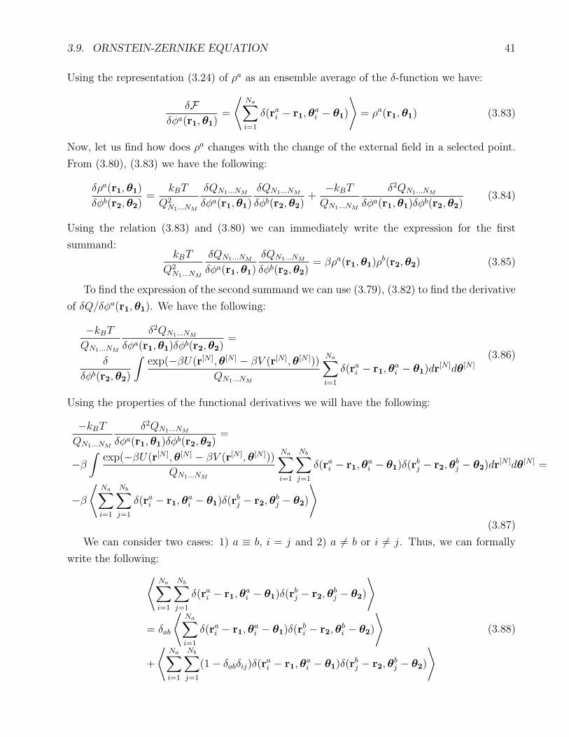
3.9. ORNSTEIN-ZERNIKE EQUATION 41
Using the representation (3.24) of ρa as an ensemble average of the δ-function we have:
δFδφa(r1,θ1)
=
⟨Na∑
i=1
δ(rai − r1,θai − θ1)
⟩
= ρa(r1,θ1) (3.83)
Now, let us find how does ρa changes with the change of the external field in a selected point.
From (3.80), (3.83) we have the following:
δρa(r1,θ1)
δφb(r2,θ2)=
kBT
Q2N1...NM
δQN1...NM
δφa(r1,θ1)
δQN1...NM
δφb(r2,θ2)+
−kBT
QN1...NM
δ2QN1...NM
δφa(r1,θ1)δφb(r2,θ2)(3.84)
Using the relation (3.83) and (3.80) we can immediately write the expression for the first
summand:kBT
Q2N1...NM
δQN1...NM
δφa(r1,θ1)
δQN1...NM
δφb(r2,θ2)= βρa(r1,θ1)ρ
b(r2,θ2) (3.85)
To find the expression of the second summand we can use (3.79), (3.82) to find the derivative
of δQ/δφa(r1,θ1). We have the following:
−kBT
QN1...NM
δ2QN1...NM
δφa(r1,θ1)δφb(r2,θ2)=
δ
δφb(r2,θ2)
∫exp(−βU(r[N ],θ[N ] − βV (r[N ],θ[N ]))
QN1...NM
Na∑
i=1
δ(rai − r1,θai − θ1)dr
[N ]dθ[N ](3.86)
Using the properties of the functional derivatives we will have the following:
−kBT
QN1...NM
δ2QN1...NM
δφa(r1,θ1)δφb(r2,θ2)=
−β
∫exp(−βU(r[N ],θ[N ] − βV (r[N ],θ[N ]))
QN1...NM
Na∑
i=1
Nb∑
j=1
δ(rai − r1,θai − θ1)δ(r
bj − r2,θ
bj − θ2)dr
[N ]dθ[N ] =
−β
⟨Na∑
i=1
Nb∑
j=1
δ(rai − r1,θai − θ1)δ(r
bj − r2,θ
bj − θ2)
⟩
(3.87)
We can consider two cases: 1) a ≡ b, i = j and 2) a 6= b or i 6= j. Thus, we can formally
write the following:
⟨Na∑
i=1
Nb∑
j=1
δ(rai − r1,θai − θ1)δ(r
bj − r2,θ
bj − θ2)
⟩
= δab
⟨Na∑
i=1
δ(rai − r1,θai − θ1)δ(r
bi − r2,θ
bi − θ2)
⟩
+
⟨Na∑
i=1
Nb∑
j=1
(1− δabδij)δ(rai − r1,θ
ai − θ1)δ(r
bj − r2,θ
bj − θ2)
⟩
(3.88)
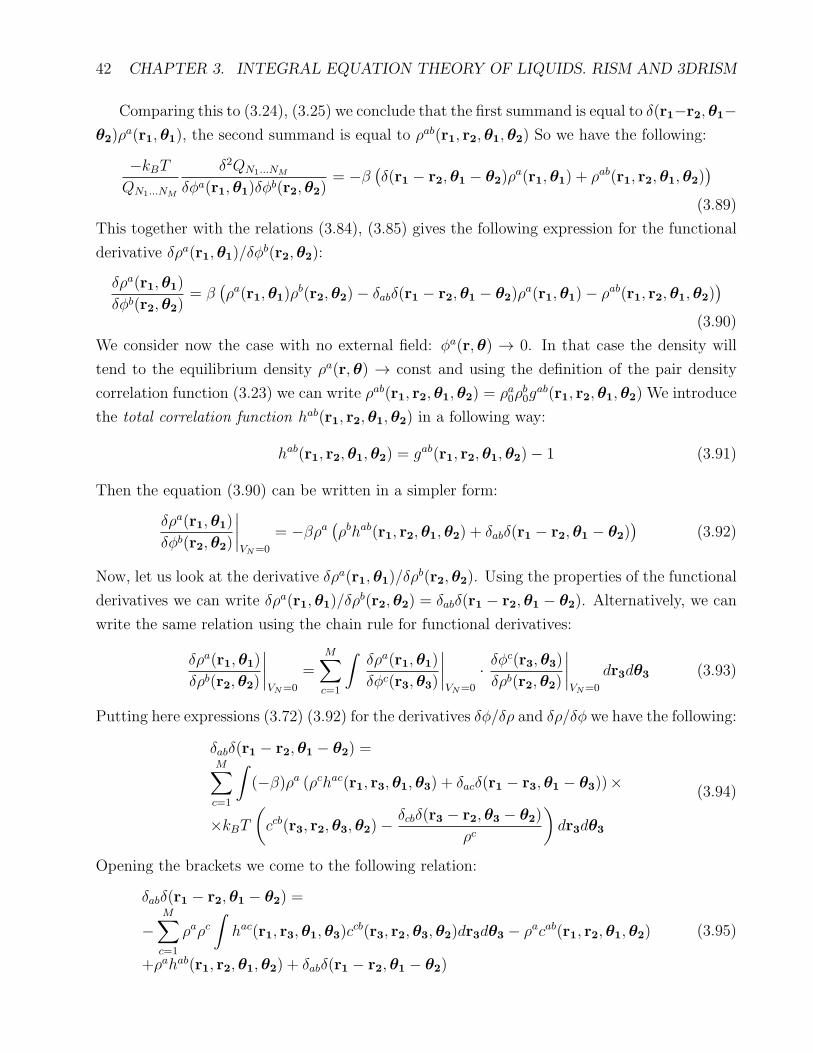
42 CHAPTER 3. INTEGRAL EQUATION THEORY OF LIQUIDS. RISM AND 3DRISM
Comparing this to (3.24), (3.25) we conclude that the first summand is equal to δ(r1−r2,θ1−θ2)ρ
a(r1,θ1), the second summand is equal to ρab(r1, r2,θ1,θ2) So we have the following:
−kBT
QN1...NM
δ2QN1...NM
δφa(r1,θ1)δφb(r2,θ2)= −β
(δ(r1 − r2,θ1 − θ2)ρ
a(r1,θ1) + ρab(r1, r2,θ1,θ2))
(3.89)
This together with the relations (3.84), (3.85) gives the following expression for the functional
derivative δρa(r1,θ1)/δφb(r2,θ2):
δρa(r1,θ1)
δφb(r2,θ2)= β
(ρa(r1,θ1)ρ
b(r2,θ2)− δabδ(r1 − r2,θ1 − θ2)ρa(r1,θ1)− ρab(r1, r2,θ1,θ2)
)
(3.90)
We consider now the case with no external field: φa(r,θ) → 0. In that case the density will
tend to the equilibrium density ρa(r,θ) → const and using the definition of the pair density
correlation function (3.23) we can write ρab(r1, r2,θ1,θ2) = ρa0ρb0g
ab(r1, r2,θ1,θ2) We introduce
the total correlation function hab(r1, r2,θ1,θ2) in a following way:
hab(r1, r2,θ1,θ2) = gab(r1, r2,θ1,θ2)− 1 (3.91)
Then the equation (3.90) can be written in a simpler form:
δρa(r1,θ1)
δφb(r2,θ2)
∣∣∣∣VN=0
= −βρa(ρbhab(r1, r2,θ1,θ2) + δabδ(r1 − r2,θ1 − θ2)
)(3.92)
Now, let us look at the derivative δρa(r1,θ1)/δρb(r2,θ2). Using the properties of the functional
derivatives we can write δρa(r1,θ1)/δρb(r2,θ2) = δabδ(r1 − r2,θ1 − θ2). Alternatively, we can
write the same relation using the chain rule for functional derivatives:
δρa(r1,θ1)
δρb(r2,θ2)
∣∣∣∣VN=0
=M∑
c=1
∫δρa(r1,θ1)
δφc(r3,θ3)
∣∣∣∣VN=0
· δφc(r3,θ3)
δρb(r2,θ2)
∣∣∣∣VN=0
dr3dθ3 (3.93)
Putting here expressions (3.72) (3.92) for the derivatives δφ/δρ and δρ/δφ we have the following:
δabδ(r1 − r2,θ1 − θ2) =M∑
c=1
∫
(−β)ρa (ρchac(r1, r3,θ1,θ3) + δacδ(r1 − r3,θ1 − θ3))×
×kBT
(
ccb(r3, r2,θ3,θ2)−δcbδ(r3 − r2,θ3 − θ2)
ρc
)
dr3dθ3
(3.94)
Opening the brackets we come to the following relation:
δabδ(r1 − r2,θ1 − θ2) =
−M∑
c=1
ρaρc∫
hac(r1, r3,θ1,θ3)ccb(r3, r2,θ3,θ2)dr3dθ3 − ρacab(r1, r2,θ1,θ2)
+ρahab(r1, r2,θ1,θ2) + δabδ(r1 − r2,θ1 − θ2)
(3.95)

3.10. CLOSURE RELATION 43
Canceling δabδ(r1 − r2,θ1 − θ2) and dividing both parts by ρa we come to the set of Ornstein-
Zernike (OZ) equations:
hab(r1, r2,θ1,θ2) = cab(r1, r2,θ1,θ2) +M∑
c=1
ρc∫
hac(r1, r3,θ1,θ3)ccb(r3, r2,θ3,θ2)dr3dθ3
a, b = 1, . . . ,M(3.96)
We note, that because the functions hab, cab, are symmetric with respect to their arguments,
we can rewrite the OZ-equations in a following way:
hba(r2, r1,θ2,θ1) = cba(r2, r1,θ2,θ1) +M∑
c=1
ρc∫
hca(r3, r1,θ3,θ1)cbc(r2, r3,θ2,θ3)dr3dθ3
(3.97)
Changing the labels a ↔ b, r1 ↔ r2, θ1 ↔ θ2 we come to the familiar form of the OZ equations:
hab(r1, r2,θ1,θ2) = cab(r1, r2,θ1,θ2) +M∑
c=1
ρc∫
cac(r1, r3,θ1,θ3)hcb(r3, r2,θ3,θ2)dr3dθ3
(3.98)
We also note, that in the uniform fluids the functions cab, hab depend only on relative shifts
between the particles but not on positions of particles themselves. Thus, the OZ equation for
uniform fluids can be written in a following form:
hab(r2−r1,θ2−θ1) = cab(r2−r1,θ2−θ1)+M∑
c=1
ρc∫
cac(r3−r1,θ3−θ1)hcb(r2−r3,θ2−θ3)dr3dθ3
(3.99)
3.10 Closure relation
Although the Ornstein-Zernike equations (3.98) are fundamental equations of the integral equa-
tion theory of liquids they are not enough to calculate the correlation functions. Equations
(3.98) give only M2 relations for 2M2 unknown correlation functions hab, cab. To make the
system of equations solvable we need to find yet M2 independent relations between the func-
tions hab, cab. Such relations can be found using the density functional theory. Let us consider
the system with the origin connected to one of the particles. Let this particle has type a. We
denote as (r0,θ0) ≡ (0,0) the coordinates of this particle. Let the particles in the system
interact via the pairwise-additive potential (3.26). In the coordinate system associated with
one of the particles we can consider that other particles move in the external field generated by
this particle. We denote this external field as V (r[N ],θ[N ]). It can be expressed in a following
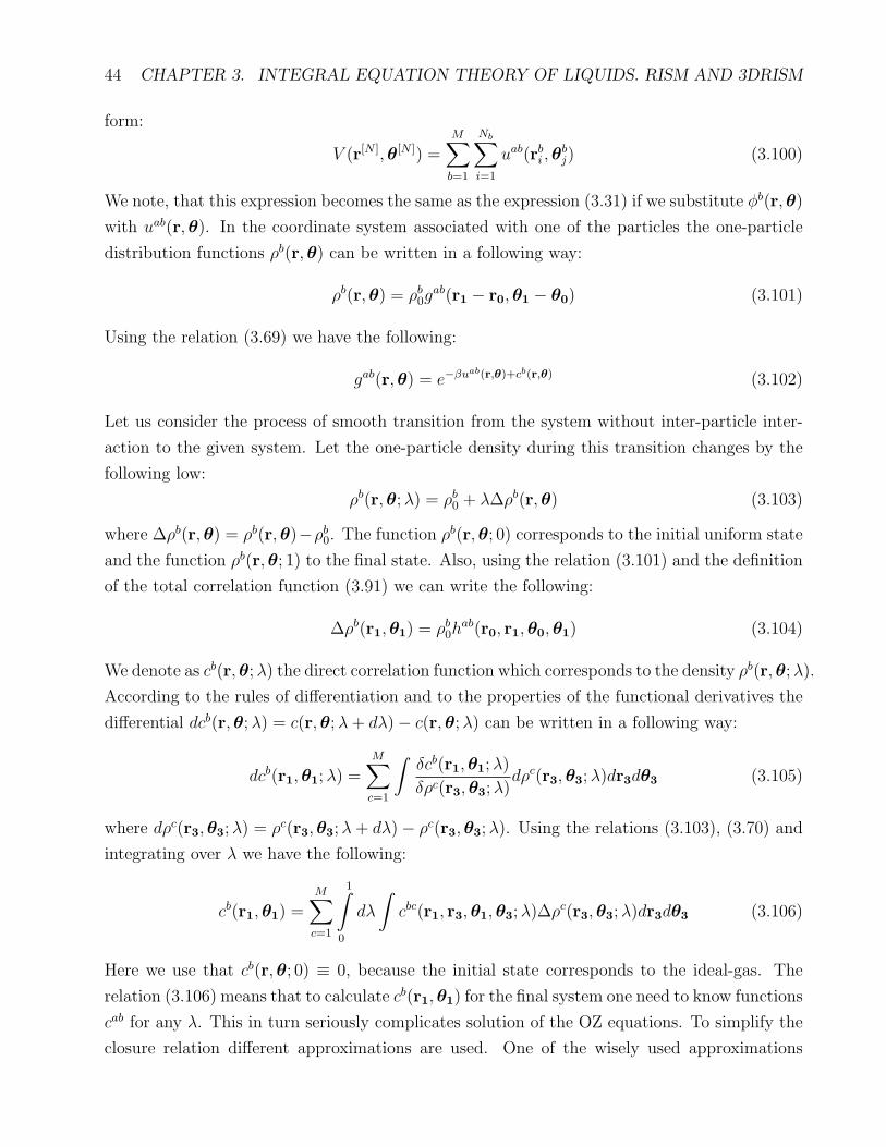
44 CHAPTER 3. INTEGRAL EQUATION THEORY OF LIQUIDS. RISM AND 3DRISM
form:
V (r[N ],θ[N ]) =M∑
b=1
Nb∑
i=1
uab(rbi ,θbj) (3.100)
We note, that this expression becomes the same as the expression (3.31) if we substitute φb(r,θ)
with uab(r,θ). In the coordinate system associated with one of the particles the one-particle
distribution functions ρb(r,θ) can be written in a following way:
ρb(r,θ) = ρb0gab(r1 − r0,θ1 − θ0) (3.101)
Using the relation (3.69) we have the following:
gab(r,θ) = e−βuab(r,θ)+cb(r,θ) (3.102)
Let us consider the process of smooth transition from the system without inter-particle inter-
action to the given system. Let the one-particle density during this transition changes by the
following low:
ρb(r,θ;λ) = ρb0 + λ∆ρb(r,θ) (3.103)
where ∆ρb(r,θ) = ρb(r,θ)−ρb0. The function ρb(r,θ; 0) corresponds to the initial uniform state
and the function ρb(r,θ; 1) to the final state. Also, using the relation (3.101) and the definition
of the total correlation function (3.91) we can write the following:
∆ρb(r1,θ1) = ρb0hab(r0, r1,θ0,θ1) (3.104)
We denote as cb(r,θ;λ) the direct correlation function which corresponds to the density ρb(r,θ;λ).
According to the rules of differentiation and to the properties of the functional derivatives the
differential dcb(r,θ;λ) = c(r,θ;λ+ dλ)− c(r,θ;λ) can be written in a following way:
dcb(r1,θ1;λ) =M∑
c=1
∫δcb(r1,θ1;λ)
δρc(r3,θ3;λ)dρc(r3,θ3;λ)dr3dθ3 (3.105)
where dρc(r3,θ3;λ) = ρc(r3,θ3;λ+ dλ)− ρc(r3,θ3;λ). Using the relations (3.103), (3.70) and
integrating over λ we have the following:
cb(r1,θ1) =M∑
c=1
1∫
0
dλ
∫
cbc(r1, r3,θ1,θ3;λ)∆ρc(r3,θ3;λ)dr3dθ3 (3.106)
Here we use that cb(r,θ; 0) ≡ 0, because the initial state corresponds to the ideal-gas. The
relation (3.106) means that to calculate cb(r1,θ1) for the final system one need to know functions
cab for any λ. This in turn seriously complicates solution of the OZ equations. To simplify the
closure relation different approximations are used. One of the wisely used approximations
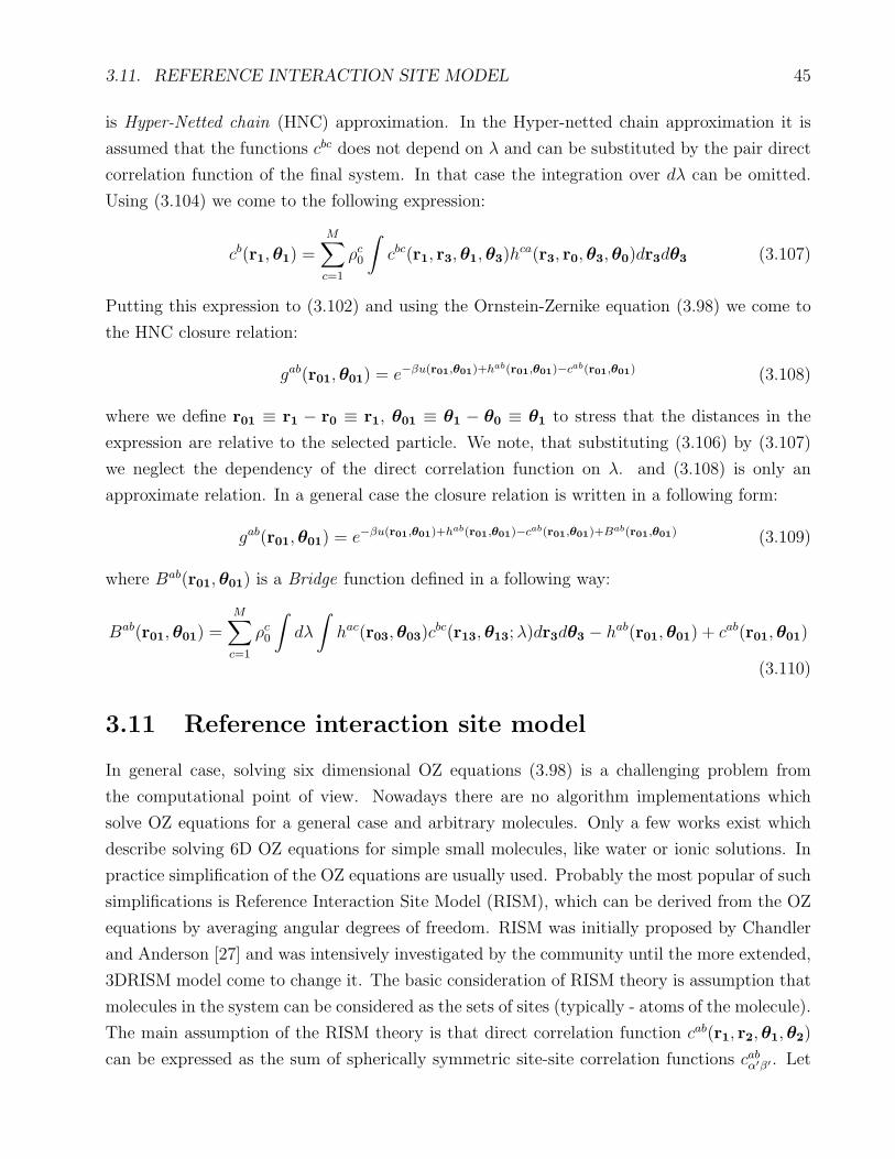
3.11. REFERENCE INTERACTION SITE MODEL 45
is Hyper-Netted chain (HNC) approximation. In the Hyper-netted chain approximation it is
assumed that the functions cbc does not depend on λ and can be substituted by the pair direct
correlation function of the final system. In that case the integration over dλ can be omitted.
Using (3.104) we come to the following expression:
cb(r1,θ1) =M∑
c=1
ρc0
∫
cbc(r1, r3,θ1,θ3)hca(r3, r0,θ3,θ0)dr3dθ3 (3.107)
Putting this expression to (3.102) and using the Ornstein-Zernike equation (3.98) we come to
the HNC closure relation:
gab(r01,θ01) = e−βu(r01,θ01)+hab(r01,θ01)−cab(r01,θ01) (3.108)
where we define r01 ≡ r1 − r0 ≡ r1, θ01 ≡ θ1 − θ0 ≡ θ1 to stress that the distances in the
expression are relative to the selected particle. We note, that substituting (3.106) by (3.107)
we neglect the dependency of the direct correlation function on λ. and (3.108) is only an
approximate relation. In a general case the closure relation is written in a following form:
gab(r01,θ01) = e−βu(r01,θ01)+hab(r01,θ01)−cab(r01,θ01)+Bab(r01,θ01) (3.109)
where Bab(r01,θ01) is a Bridge function defined in a following way:
Bab(r01,θ01) =M∑
c=1
ρc0
∫
dλ
∫
hac(r03,θ03)cbc(r13,θ13;λ)dr3dθ3 − hab(r01,θ01) + cab(r01,θ01)
(3.110)
3.11 Reference interaction site model
In general case, solving six dimensional OZ equations (3.98) is a challenging problem from
the computational point of view. Nowadays there are no algorithm implementations which
solve OZ equations for a general case and arbitrary molecules. Only a few works exist which
describe solving 6D OZ equations for simple small molecules, like water or ionic solutions. In
practice simplification of the OZ equations are usually used. Probably the most popular of such
simplifications is Reference Interaction Site Model (RISM), which can be derived from the OZ
equations by averaging angular degrees of freedom. RISM was initially proposed by Chandler
and Anderson [27] and was intensively investigated by the community until the more extended,
3DRISM model come to change it. The basic consideration of RISM theory is assumption that
molecules in the system can be considered as the sets of sites (typically - atoms of the molecule).
The main assumption of the RISM theory is that direct correlation function cab(r1, r2,θ1,θ2)
can be expressed as the sum of spherically symmetric site-site correlation functions cabα′β′ . Let
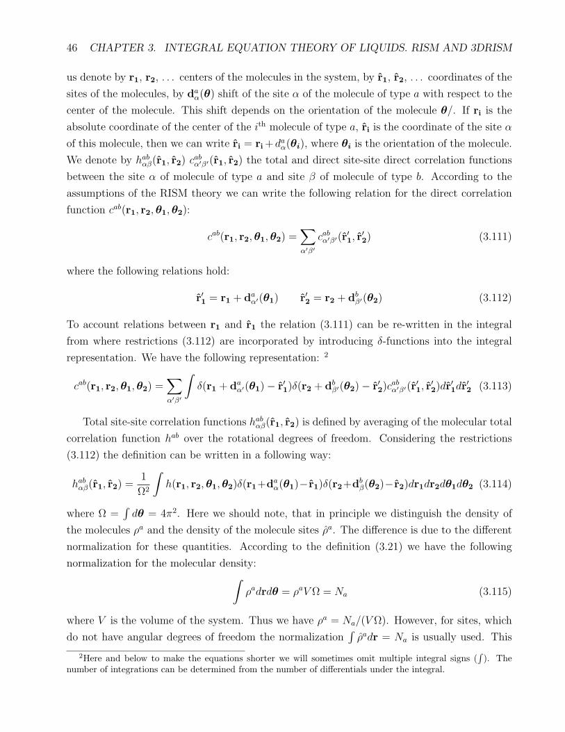
46 CHAPTER 3. INTEGRAL EQUATION THEORY OF LIQUIDS. RISM AND 3DRISM
us denote by r1, r2, . . . centers of the molecules in the system, by r1, r2, . . . coordinates of the
sites of the molecules, by daα(θ) shift of the site α of the molecule of type a with respect to the
center of the molecule. This shift depends on the orientation of the molecule θ/. If ri is the
absolute coordinate of the center of the ith molecule of type a, ri is the coordinate of the site α
of this molecule, then we can write ri = ri+daα(θi), where θi is the orientation of the molecule.
We denote by habαβ(r1, r2) c
abα′β′(r1, r2) the total and direct site-site direct correlation functions
between the site α of molecule of type a and site β of molecule of type b. According to the
assumptions of the RISM theory we can write the following relation for the direct correlation
function cab(r1, r2,θ1,θ2):
cab(r1, r2,θ1,θ2) =∑
α′β′
cabα′β′(r′1, r′2) (3.111)
where the following relations hold:
r′1 = r1 + daα′(θ1) r′2 = r2 + db
β′(θ2) (3.112)
To account relations between r1 and r1 the relation (3.111) can be re-written in the integral
from where restrictions (3.112) are incorporated by introducing δ-functions into the integral
representation. We have the following representation: 2
cab(r1, r2,θ1,θ2) =∑
α′β′
∫
δ(r1 + daα′(θ1)− r′1)δ(r2 + db
β′(θ2)− r′2)cabα′β′(r′1, r
′2)dr
′1dr
′2 (3.113)
Total site-site correlation functions habαβ(r1, r2) is defined by averaging of the molecular total
correlation function hab over the rotational degrees of freedom. Considering the restrictions
(3.112) the definition can be written in a following way:
habαβ(r1, r2) =
1
Ω2
∫
h(r1, r2,θ1,θ2)δ(r1+daα(θ1)−r1)δ(r2+db
β(θ2)−r2)dr1dr2dθ1dθ2 (3.114)
where Ω =∫dθ = 4π2. Here we should note, that in principle we distinguish the density of
the molecules ρa and the density of the molecule sites ρa. The difference is due to the different
normalization for these quantities. According to the definition (3.21) we have the following
normalization for the molecular density:∫
ρadrdθ = ρaV Ω = Na (3.115)
where V is the volume of the system. Thus we have ρa = Na/(V Ω). However, for sites, which
do not have angular degrees of freedom the normalization∫ρadr = Na is usually used. This
2Here and below to make the equations shorter we will sometimes omit multiple integral signs (∫). The
number of integrations can be determined from the number of differentials under the integral.
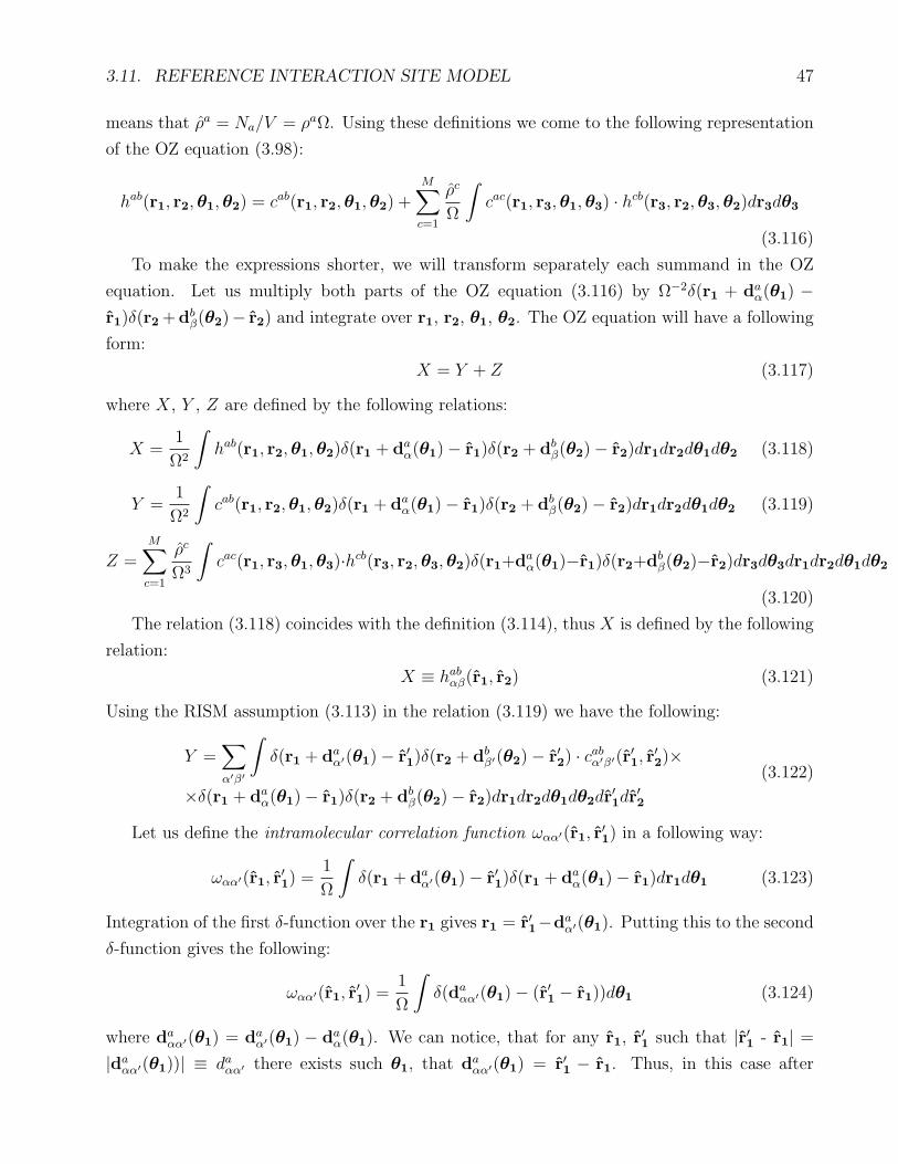
3.11. REFERENCE INTERACTION SITE MODEL 47
means that ρa = Na/V = ρaΩ. Using these definitions we come to the following representation
of the OZ equation (3.98):
hab(r1, r2,θ1,θ2) = cab(r1, r2,θ1,θ2) +M∑
c=1
ρc
Ω
∫
cac(r1, r3,θ1,θ3) · hcb(r3, r2,θ3,θ2)dr3dθ3
(3.116)
To make the expressions shorter, we will transform separately each summand in the OZ
equation. Let us multiply both parts of the OZ equation (3.116) by Ω−2δ(r1 + daα(θ1) −
r1)δ(r2 +dbβ(θ2)− r2) and integrate over r1, r2, θ1, θ2. The OZ equation will have a following
form:
X = Y + Z (3.117)
where X, Y , Z are defined by the following relations:
X =1
Ω2
∫
hab(r1, r2,θ1,θ2)δ(r1 + daα(θ1)− r1)δ(r2 + db
β(θ2)− r2)dr1dr2dθ1dθ2 (3.118)
Y =1
Ω2
∫
cab(r1, r2,θ1,θ2)δ(r1 + daα(θ1)− r1)δ(r2 + db
β(θ2)− r2)dr1dr2dθ1dθ2 (3.119)
Z =M∑
c=1
ρc
Ω3
∫
cac(r1, r3,θ1,θ3)·hcb(r3, r2,θ3,θ2)δ(r1+daα(θ1)−r1)δ(r2+db
β(θ2)−r2)dr3dθ3dr1dr2dθ1dθ2
(3.120)
The relation (3.118) coincides with the definition (3.114), thus X is defined by the following
relation:
X ≡ habαβ(r1, r2) (3.121)
Using the RISM assumption (3.113) in the relation (3.119) we have the following:
Y =∑
α′β′
∫
δ(r1 + daα′(θ1)− r′1)δ(r2 + db
β′(θ2)− r′2) · cabα′β′(r′1, r′2)×
×δ(r1 + daα(θ1)− r1)δ(r2 + db
β(θ2)− r2)dr1dr2dθ1dθ2dr′1dr
′2
(3.122)
Let us define the intramolecular correlation function ωαα′(r1, r′1) in a following way:
ωαα′(r1, r′1) =
1
Ω
∫
δ(r1 + daα′(θ1)− r′1)δ(r1 + da
α(θ1)− r1)dr1dθ1 (3.123)
Integration of the first δ-function over the r1 gives r1 = r′1−daα′(θ1). Putting this to the second
δ-function gives the following:
ωαα′(r1, r′1) =
1
Ω
∫
δ(daαα′(θ1)− (r′1 − r1))dθ1 (3.124)
where daαα′(θ1) = da
α′(θ1) − daα(θ1). We can notice, that for any r1, r
′1 such that |r′1 - r1| =
|daαα′(θ1))| ≡ daαα′ there exists such θ1, that da
αα′(θ1) = r′1 − r1. Thus, in this case after
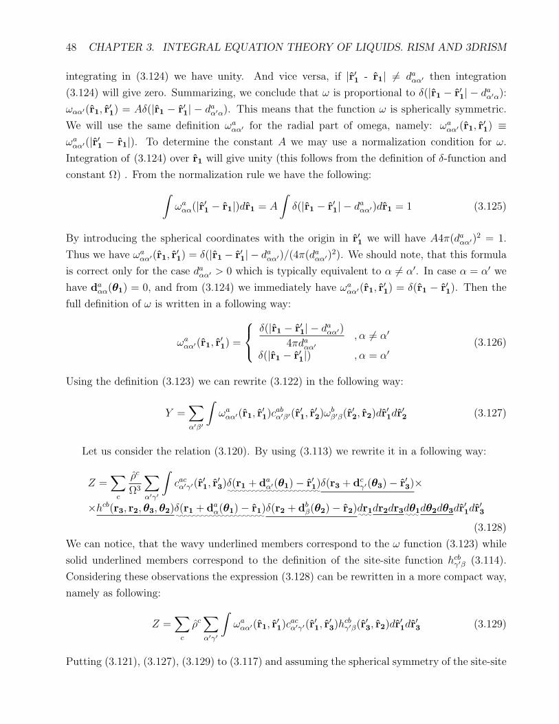
48 CHAPTER 3. INTEGRAL EQUATION THEORY OF LIQUIDS. RISM AND 3DRISM
integrating in (3.124) we have unity. And vice versa, if |r′1 - r1| 6= daαα′ then integration
(3.124) will give zero. Summarizing, we conclude that ω is proportional to δ(|r1 − r′1| − daα′α):
ωαα′(r1, r′1) = Aδ(|r1 − r′1| − daα′α). This means that the function ω is spherically symmetric.
We will use the same definition ωaαα′ for the radial part of omega, namely: ωa
αα′(r1, r′1) ≡
ωaαα′(|r′1 − r1|). To determine the constant A we may use a normalization condition for ω.
Integration of (3.124) over r1 will give unity (this follows from the definition of δ-function and
constant Ω) . From the normalization rule we have the following:
∫
ωaαα(|r′1 − r1|)dr1 = A
∫
δ(|r1 − r′1| − daαα′)dr1 = 1 (3.125)
By introducing the spherical coordinates with the origin in r′1 we will have A4π(daαα′)2 = 1.
Thus we have ωaαα′(r1, r
′1) = δ(|r1 − r′1| − daαα′)/(4π(daαα′)2). We should note, that this formula
is correct only for the case daαα′ > 0 which is typically equivalent to α 6= α′. In case α = α′ we
have daαα(θ1) = 0, and from (3.124) we immediately have ωa
αα′(r1, r′1) = δ(r1 − r′1). Then the
full definition of ω is written in a following way:
ωaαα′(r1, r
′1) =
δ(|r1 − r′1| − daαα′)
4πdaαα′
, α 6= α′
δ(|r1 − r′1|) , α = α′(3.126)
Using the definition (3.123) we can rewrite (3.122) in the following way:
Y =∑
α′β′
∫
ωaαα′(r1, r
′1)c
abα′β′(r′1, r
′2)ω
bβ′β(r
′2, r2)dr
′1dr
′2 (3.127)
Let us consider the relation (3.120). By using (3.113) we rewrite it in a following way:
Z =∑
c
ρc
Ω3
∑
α′γ′
∫
cacα′γ′(r′1, r′3)δ(r1 + da
α′(θ1)− r′1)
δ(r3 + dcγ′(θ3)− r′3)×
×hcb(r3, r2,θ3,θ2)δ(r1 + daα(θ1)− r1)
δ(r2 + dbβ(θ2)− r2)dr1
dr2dr3dθ1
dθ2dθ3dr′1dr
′3
(3.128)
We can notice, that the wavy underlined members correspond to the ω function (3.123) while
solid underlined members correspond to the definition of the site-site function hcbγ′β (3.114).
Considering these observations the expression (3.128) can be rewritten in a more compact way,
namely as following:
Z =∑
c
ρc∑
α′γ′
∫
ωaαα′(r1, r
′1)c
acα′γ′(r′1, r
′3)h
cbγ′β(r
′3, r2)dr
′1dr
′3 (3.129)
Putting (3.121), (3.127), (3.129) to (3.117) and assuming the spherical symmetry of the site-site

3.12. CLOSURE RELATION FOR THE RISM EQUATIONS 49
correlation function we obtain the RISM equations, namely:
habαβ(|r2 − r1|) =
∑
α′β′
∫
ωaαα′(|r′1 − r1|)cabα′β′(|r′2 − r′1|)ωb
β′β(|r2 − r′2|)dr′1dr′2
+∑
c
ρc∑
α′γ′
∫
ωaαα′(|r′1 − r1|)cacα′γ′(|r′3 − r′1|)hcb
γ′β(|r2 − r′3|)dr′1dr′3(3.130)
3.12 Closure relation for the RISM equations
Similarly to the OZ equation (3.98), RISM equation need to be comprised with the closure
relation. In the RISM theory it is assumed that sites interact to each other independently.
Thus, the closure relation can be written for each pair of sites independently. By analogy to
(3.109) we can write the set of site-site closure relations:
habsα(r) + 1 = e−βuab
sα(r)+habsα(r)−cabsα(r)+Bab
sα(r) (3.131)
where uabsα(r) is the site-site interaction potential, Bab
sα(r) is the site-site bridge function. By
analogy to the six-dimensional HNC approximation (3.108) we can write the site-site HNC
closure in a following way[52]:
habsα(r) + 1 = e−βuab
sα(r)+habsα(r)−cabsα(r) (3.132)
We note, that this is quite rude approximation. There are two sources of errors: 1) As in the
six-dimensional case neglecting the bridge functional leads to some errors 2) The assumption,
that sites interact independently introduces even more RISM-specific errors. Typically, by using
HNC approximation one cannot get good quantitative agreements of the calculated physical
quantities to the experimentally measured quantities or quantities calculated using molecular
simulations. Moreover: overestimation of the first peaks of the total correlation functions
often lead to divergence of the numerical algorithms which solve RISM equations. There are
several different bridge approximations. To mention few: Percus-Yevick bridge [103], Martynov-
Sarkisov approximation [104], Modified Verlet bridge[105] and others[106]. The search for new
bridge functionals is currently actively performed [107, 108]. For some specific conditions, for
example for Ornstein-Zernike equations for mixtures of Lennard-Jones spheres, the mentioned
above bridges can give satisfactorily results. However, the functional which is good for a
wide range of different systems is still not known. In the current work it is not our goal to
find an universal bridge. However, it is necessary to use the closure which at least warrant
the convergence of the algorithm (as was mentioned above, HNC closure is not good in this
respect). To improve convergence of the algorithm one can linearize the exponent in the closure
relation (3.131) when the argument of the exponent is positive. This method was proposed by
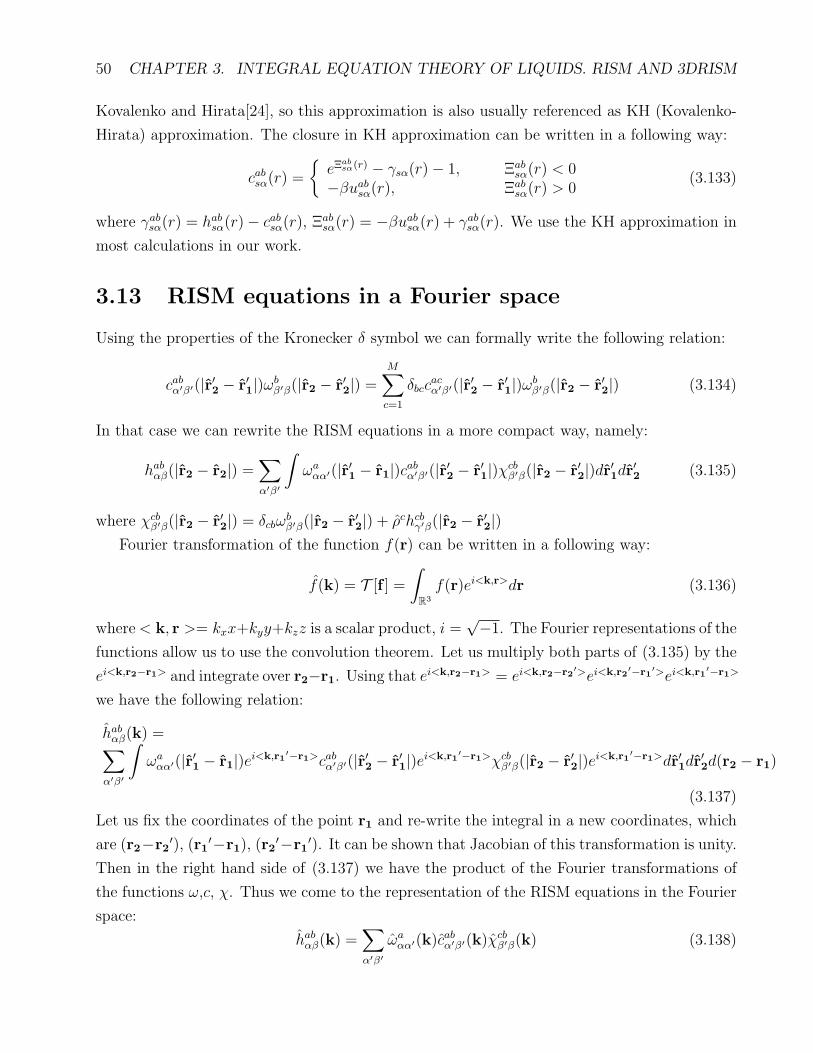
50 CHAPTER 3. INTEGRAL EQUATION THEORY OF LIQUIDS. RISM AND 3DRISM
Kovalenko and Hirata[24], so this approximation is also usually referenced as KH (Kovalenko-
Hirata) approximation. The closure in KH approximation can be written in a following way:
cabsα(r) =
eΞabsα(r) − γsα(r)− 1, Ξab
sα(r) < 0−βuab
sα(r), Ξabsα(r) > 0
(3.133)
where γabsα(r) = hab
sα(r)− cabsα(r), Ξabsα(r) = −βuab
sα(r) + γabsα(r). We use the KH approximation in
most calculations in our work.
3.13 RISM equations in a Fourier space
Using the properties of the Kronecker δ symbol we can formally write the following relation:
cabα′β′(|r′2 − r′1|)ωbβ′β(|r2 − r′2|) =
M∑
c=1
δbccacα′β′(|r′2 − r′1|)ωb
β′β(|r2 − r′2|) (3.134)
In that case we can rewrite the RISM equations in a more compact way, namely:
habαβ(|r2 − r2|) =
∑
α′β′
∫
ωaαα′(|r′1 − r1|)cabα′β′(|r′2 − r′1|)χcb
β′β(|r2 − r′2|)dr′1dr′2 (3.135)
where χcbβ′β(|r2 − r′2|) = δcbω
bβ′β(|r2 − r′2|) + ρchcb
γ′β(|r2 − r′2|)Fourier transformation of the function f(r) can be written in a following way:
f(k) = T [f ] =
∫
R3
f(r)ei<k,r>dr (3.136)
where< k, r >= kxx+kyy+kzz is a scalar product, i =√−1. The Fourier representations of the
functions allow us to use the convolution theorem. Let us multiply both parts of (3.135) by the
ei<k,r2−r1> and integrate over r2−r1. Using that ei<k,r2−r1> = ei<k,r2−r2
′>ei<k,r2′−r1′>ei<k,r1′−r1>
we have the following relation:
habαβ(k) =∑
α′β′
∫
ωaαα′(|r′1 − r1|)ei<k,r1′−r1>cabα′β′(|r′2 − r′1|)ei<k,r1′−r1>χcb
β′β(|r2 − r′2|)ei<k,r1′−r1>dr′1dr′2d(r2 − r1)
(3.137)
Let us fix the coordinates of the point r1 and re-write the integral in a new coordinates, which
are (r2−r2′), (r1
′−r1), (r2′−r1
′). It can be shown that Jacobian of this transformation is unity.
Then in the right hand side of (3.137) we have the product of the Fourier transformations of
the functions ω,c, χ. Thus we come to the representation of the RISM equations in the Fourier
space:
habαβ(k) =
∑
α′β′
ωaαα′(k)cabα′β′(k)χcb
β′β(k) (3.138)

3.14. REDUCING THE RISM EQUATIONS TO THE SYSTEMOFONE-DIMENSIONAL EQUATIONS
3.14 Reducing the RISM equations to the system of
one-dimensional equations
Formally, Fourier transformations in (3.138) are three-dimensional. However, there is no need to
numerically calculate the three dimensional Fourier transformation of the spherically symmetric
functions . The Fourier transform of the spherically symmetric function f(|r|) is spherically
symmetric itself. It is easy to proof. Let |k1| = |k2|. Then there is a rotation which transforms
the vector k1 into the vector k2. Let A be the matrix of this rotation, i.e k2 = Ak1. The
Fourier transform of the radially symmetric function f(|r|) is written in the following way:
f(k1) =
∫
eik1T rf(|r|)dr (3.139)
Let us rewrite this relation in a new coordinates x = Ar. Due to the properties of the rotation
matrix the Jacobian of such transformation is det(A) = 1, thus dx = dr. Also, it is known that
for matrices which represent rotation it holds A−1 = AT , thus r = ATx. Also, the rotation
do not change the size of the vectors, so |r| = |Ar| = |x|. Using all this knowledge we rewrite
(3.139) in a following way:
f(k1) =
∫
eik1TATxf(|x|)dx (3.140)
Using that k1TAT = (Ak1)
T = k2T we have the definition of the Fourier transform in the
point k2 in the right hand side of the equation. Thus f(k1) = f(k2) and f(k) is spherically
symmetric. This allows us to rewrite (3.138) for radial part k = |k|:
habαβ(k) =
∑
α′β′
ωaαα′(k)cabα′β′(k)χcb
β′β(k) (3.141)
3.15 Bessel-Fourier transformation
The knowledge that the 3D Fourier transform of spherically symmetric function is spherically
symmetric does not give by itself the algorithm how to calculate this Fourier transform in a
simple way. Let us obtain this formula. Because the Fourier transform is spherically symmetric
we only need to know its values along one of the axis. Let us calculate the values f(0, 0, kz).
The Fourier transform of the function f(x, y, z) is written in a following way:
f(k) = f(kx, ky, kz) =
∞∫
−∞
∞∫
−∞
∞∫
−∞
f(r)eikxx+ikyy+ikzzdxdydz (3.142)
where i =√−1. The values at the kz axis are:
f(0, 0, kz) =
∞∫
−∞
∞∫
−∞
∞∫
−∞
f(r)eikzzdxdydz (3.143)

52 CHAPTER 3. INTEGRAL EQUATION THEORY OF LIQUIDS. RISM AND 3DRISM
For the sake of simplicity we denote k ≡ kz, f(0, 0, kz) ≡ f(k). Transferring to the spherical
coordinates we have the following:
f(k) =
∞∫
0
π∫
0
π∫
−π
f(r)eikr cos θr2 sin θdrdθdφ (3.144)
where x = r sin θ cosφ, y = r sin θ sinφ, z = r cos θ, dxdydz = r2 sin θdrdθdφ. Integration over
φ gives 2π. Introducing the variable ξ = cosθ, dξ = − sin θdθ, ξ ∈ [cos 0; cos π] = [1;−1], we
have the following:
f(k) = −2π
∞∫
0
−1∫
1
f(r)eikrξr2dξdr (3.145)
After calculation of the internal integral over ξ we have the following:
f(k) = 2π
∞∫
0
f(r)
(eikr − e−ikr
ikr
)
r2dr (3.146)
Using the Euler’s formula sinα = eiα−e−iα
2iwe obtain the following transformation:
f(k) =4π
k
∞∫
0
f(r)r sin krdr (3.147)
This transformation is called the Bessel-Fourier transformation.
3.16 Inverse Bessel-Fourier transformation
Expression (3.147) can be re-written in a form of the sine transform of the function rf(r),
namely:
kf(k) = 4π
∞∫
0
(rf(r)) sin krdr (3.148)
Because the sine transform is inverse to itself in a general case the inverse Bessel-Fourier
transform can be written in a following way:
r′f(r′) = A
∞∫
0
(
kf(k))
sin kr′dk (3.149)
where A is a normalization constant. It is necessary to note that one need to be cautious in
calculations. It is known that the integral over sin kr has only conditional convergence at the
interval [0;∞). This means that the value of the integral depends on the discretization of the

3.16. INVERSE BESSEL-FOURIER TRANSFORMATION 53
function. In practice one typically uses the discretization on the equispaced grid. Let us assume
that the function f(r) has the support [0;R] and is defined at the points with the discretization
step ∆r = RN. Assuming that the function have some finite integral we can write it using the
Dirac delta-function:
f(r) =N∑
n=1
f(rn)δ(r − rn)∆r =R
N
N∑
n=1
f(rn)δ(r − rn) (3.150)
Putting (3.150) to the transformation (3.148) we obtain the discrete Bessel-Fourier transform,
namely:
kf(k) = 4π
∞∫
0
r
N∑
n=1
f(rn)δ(r − rn)∆r sin krdr (3.151)
Using the properties of the δ-function we have the following:
kf(k) = 4πR
N
N∑
n=1
nR
Nf(
nR
N) sin k
nR
N(3.152)
Let r′ = m∆r = mRN, m ∈ N. Let us change the infinite integration limit in the expression
(3.149) by the finite number πNR. As we show below such a value is necessary for orthogonality
of the eigenfunctions sin k nRN. Equation (3.149) is transformed to the following expression:
mR
Nf(
mR
N) = A
πNR∫
0
kf(k) sin kmR
Ndk (3.153)
Putting (3.152) to (3.153) we have the following:
mR
Nf(
mR
N) = 4π
R
NA
N∑
n=1
nR
Nf(
nR
N)
πNR∫
0
sin knR
Nsin k
mR
Ndk (3.154)
The set of the functions sin knRN
, n ∈ N, k ∈ R is orthogonal in a sense of the L2 scalar
product on the interval k ∈ [0; πNR]. If m 6= n we have the following:
πNR∫
0
sin knR
Nsin k
mR
Ndk =
1
2
πNR∫
0
cos k(m− n)R
N− cos k
(m+ n)R
Ndk =
1
2
N
m− nsin
π(m− n)NR
RN− 1
2
N
m+ nsin
π(m+ n)NR
RN= 0
(3.155)

54 CHAPTER 3. INTEGRAL EQUATION THEORY OF LIQUIDS. RISM AND 3DRISM
When m = n we have the following:
πNR∫
0
sin2 nR
Ndk =
1
2
πNR∫
0
(
1− cos2knR
N
)
dk =πN
2R(3.156)
Combining (3.155) and (3.156) we write the following:
πNR∫
0
sin knR
Nsin k
mR
Ndk =
πN
2Rδmn (3.157)
where δmn is a Kronecker delta.
Putting (3.157) into (3.154) and using that∑
nnRNf(nR
N)δmn = mR
Nf(mR
N) we have the fol-
lowing:mR
Nf(
mR
N) = 4πA
R
N
mR
Nf(
mR
N)πN
2R(3.158)
Because this equality is true for any function f(r) we conclude that the following relation holds:
1 = 4πAR
N
πN
2R(3.159)
From this relation we can express the coefficient A:
A =1
2π2(3.160)
Taking a limit N → ∞ and dividing both parts of the expression (3.153) by r′ = mRN
we
obtain the following expression for the inverse Bessel-Fourier transform:
f(r′) =1
2πr′
∞∫
0
kf(k) sin kr′dk (3.161)
We need to note, that one should be cautious using expressions (3.147),(3.161) because on
the infinite gird the results may depend on a grid. To avoid problems it is better to use discrete
formulae (3.152),(3.153).
Often for the calculation of the integral over k in the equation (3.153) the zero-order inte-
gration approximation is used. In that case to cover the interval (0; πNR) one need to choose the
grid step in the Fourier space ∆k considering the relation N∆k = πNR. This gives the following
relation for the ∆k
∆k =π
R(3.162)
where R is a top boundary of the support of the function f(r). The step of the equispaced
N -point grid in the real space is ∆r = RN. Thus from the expression (3.162) we find the relation
between the steps in the real and Fourier spaces:
∆r∆k =π
N(3.163)

3.17. RISM EQUATIONS IN A MATRIX REPRESENTATION 55
We define km = m∆k, rn = n∆r. Using (3.163) we obtain the following:
rnkm =πmn
N(3.164)
In these definitions the forward and inverse Bessel-Fourier transforms are defined by the for-
mulae (3.165), (3.166) correspondingly.
f(km) =4π
km
N∑
n=1
f(rn)rn sin(πmn
N)∆r (3.165)
f(rm) =1
π2rn
N∑
m=1
f(km)km sin(πmn
N)∆k (3.166)
There are effective FFT-based algorithms which are able to calculate the expressions (3.165),
(3.166) in time proportional to NlogN .
3.17 RISM equations in a matrix representation
Let the molecule of type a has Ka sites. We can define the following matrices of the correlation
functions:
Hab(k) = [habsα(k)]Ka×Kb
=
hab11(k) . . . hab
1Kb(k)
.... . .
...
habKa1
(k) . . . habKaKb
(k)
(3.167)
Cab = [cabsα(k)]Ka×Kb=
cab11(k) . . . cab1Kb(k)
.... . .
...cabKa1
(k) . . . cabKaKb(k)
(3.168)
Wa = [ωasα(k)]Ka×Ka
=
ωa11(k) . . . ωa
1Ka(k)
.... . .
...ωaKa1
(k) . . . ωaKaKa
(k)
(3.169)
Then using the definition of the matrix multiplication we can rewrite the RISM equations
(3.141) in a following way:
Hab(k) =∑
c
Wa(k)Cac(k)Xcb(k) (3.170)
where Xcb(k) = δcbWb(k) + ρcHcb(k)
We define the matrices H, C, W in a following way:
H(k) =
H11(k) . . . H1M(k)...
. . ....
HM1(k) . . . HMM(k)
(3.171)
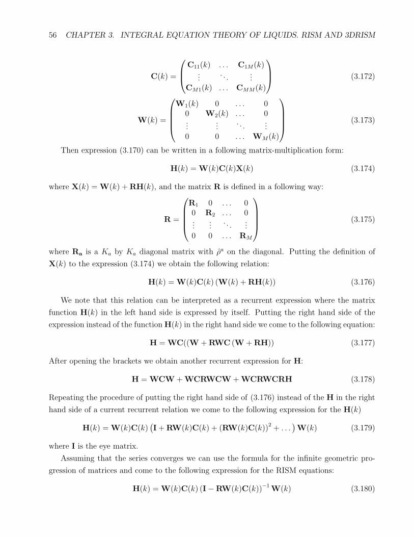
56 CHAPTER 3. INTEGRAL EQUATION THEORY OF LIQUIDS. RISM AND 3DRISM
C(k) =
C11(k) . . . C1M(k)...
. . ....
CM1(k) . . . CMM(k)
(3.172)
W(k) =
W1(k) 0 . . . 00 W2(k) . . . 0...
.... . .
...0 0 . . . WM(k)
(3.173)
Then expression (3.170) can be written in a following matrix-multiplication form:
H(k) = W(k)C(k)X(k) (3.174)
where X(k) = W(k) +RH(k), and the matrix R is defined in a following way:
R =
R1 0 . . . 00 R2 . . . 0...
.... . .
...0 0 . . . RM
(3.175)
where Ra is a Ka by Ka diagonal matrix with ρa on the diagonal. Putting the definition of
X(k) to the expression (3.174) we obtain the following relation:
H(k) = W(k)C(k) (W(k) +RH(k)) (3.176)
We note that this relation can be interpreted as a recurrent expression where the matrix
function H(k) in the left hand side is expressed by itself. Putting the right hand side of the
expression instead of the functionH(k) in the right hand side we come to the following equation:
H = WC((W +RWC (W +RH)) (3.177)
After opening the brackets we obtain another recurrent expression for H:
H = WCW +WCRWCW +WCRWCRH (3.178)
Repeating the procedure of putting the right hand side of (3.176) instead of the H in the right
hand side of a current recurrent relation we come to the following expression for the H(k)
H(k) = W(k)C(k)(I+RW(k)C(k) + (RW(k)C(k))2 + . . .
)W(k) (3.179)
where I is the eye matrix.
Assuming that the series converges we can use the formula for the infinite geometric pro-
gression of matrices and come to the following expression for the RISM equations:
H(k) = W(k)C(k) (I−RW(k)C(k))−1W(k) (3.180)

3.18. 3DRISM EQUATIONS 57
3.18 3DRISM equations
As it was mentioned above for the solvation free energy calculations one need to know the cor-
relation functions between the solute and solvent molecules where solute is at infinite dilution.
To calculate these functions we consider the model system where the single solute molecule is
fixed in the origin and surrounded by moving solvent molecules. We will refer to the solute
molecule using the superscript index 0. Considering that the solute is infinitely diluted we can
write the OZ equations (3.98) for the solute-solvent correlation functions in a following way:
h0a(r0, r2,θ0,θ2) = c0a(r0, r2,θ0,θ2) +M∑
c=1
ρc
Ω
∫
c0c(r0, r3,θ0,θ3)hca(r3, r2,θ3,θ2)dr3dθ3
(3.181)
where (r0,θ0) at the coordinates of the solute molecule.
It was discussed that due to a computational complexity solving of OZ equations is not the
best method for SFE calculations. From the other hand it is also known that the RISM approx-
imation introduces many additional errors and is unable to treat correctly the molecule geom-
etry. The compromise between these methods is so-called 3DRISM -approximation, where the
solvent molecules are teated in a RISM approximation, while the solute is a three-dimensional
object[69]. To obtain the RISM equations we introduce the solute-site total and direct corre-
lation functions, which are averaged over the solvent rotational degrees of freedom molecular
correlation functions. By the analogy to the site-site correlation functions (3.114) the total
solute-site correlation function haα(r) of site α of molecule a is defined in a following way:
haα(rα) =
1
Ω
∫
h0a(r0, r2,θ0,θ2)δ(r2 + daα(θ2)− r)dr2dθ2 (3.182)
where daα(θ) is a displacement of the site α of the molecule of type a with respect to the center
of the molecule if the orientation of the molecule is defined by the Euler angles θ. The main
assumption of the 3DRISM theory is that the molecular direct correlation functions c0a can be
represented as a sum of solute-site direct correlation functions caα′ , namely:
c(r0, r2,θ0,θ2) =∑
α′
∫
caα′(r′)δ(r2 + daα(θ2)− r′)dr′ (3.183)
Multiplying (3.181) by Ω−1δ(r2 + daα(θ2) − r), integrating over the r2, θ2 and using (3.182),
(3.183) we come to the following relation:
haα(r) = X + Y (3.184)
where X, Y are defined by the following relations:
X =∑
α′
1
Ω
∫
caα′(r)δ(r2 + daα′(θ2)− r)δ(r2 + da
α(θ2)− r)dr′dr2dθ2 (3.185)
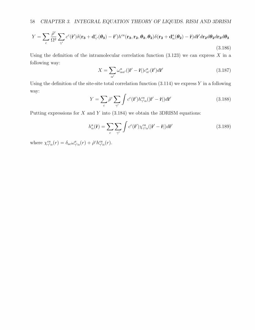
58 CHAPTER 3. INTEGRAL EQUATION THEORY OF LIQUIDS. RISM AND 3DRISM
Y =∑
c
ρc
Ω2
∑
γ′
cc(r′)δ(r3 + dcγ′(θ3)− r′)hca(r3, r2,θ3,θ2)δ(r2 + da
α(θ2)− r)dr′dr2dθ2dr3dθ3
(3.186)
Using the definition of the intramolecular correlation function (3.123) we can express X in a
following way:
X =∑
α′
ωaαα′(|r′ − r|)caα′(r′)dr′ (3.187)
Using the definition of the site-site total correlation function (3.114) we express Y in a following
way:
Y =∑
c
ρc∑
γ′
∫
cc(r′)hcaγ′α(|r′ − r|)dr′ (3.188)
Putting expressions for X and Y into (3.184) we obtain the 3DRISM equations:
haα(r) =
∑
c
∑
γ′
∫
cc(r′)χcaγ′α(|r′ − r|)dr′ (3.189)
where χcaγ′α(r) = δacω
aγ′α(r) + ρchca
γ′α(r).

Chapter 4
Solvation Free Energy Calculation in
RISM and 3DRISM
In this chapter the ways to calculate the solvation free energy in the RISM and 3DRISM ap-
proximations are discussed. The main reference for this chapter is Ref. [24]. The description of
the semi-empirical solvation free energy expressions can be found in Refs. [64],[65],[109],[66],[74]
4.1 Thermodynamic integration method for calculation
of the free energy change
Although we have the formal definition of the Helmholtz free energy (2.79), it is difficult to use
it in practice. The partition function (3.7) is formally defined as the 12N -fold integral, where
N is the number of particles in the system, which is a very big number. However, we rarely
need to find the total free energy of the system. For most of applications one need to know only
relative free energy change in one or another process. To find such changes one can use the
thermodynamic integration method [110]. In this method it is assumed that the potential energy
of the system depends on some parameter λ. When λ = 0 the potential is the same as the
potential in the initial state, when λ = 1 the potential coincides with the potential of the final
state of the system. We would like to find a convenient expression for the free energy change.
To do it we find a derivative of the free energy (2.79) over the λ. Using the definitions of the
configurational integral (3.13) and partition function (3.14) we obtain the following relation:
∂F∂λ
=−kBT
QN1...NM
∂QN1...NM
∂λ= −kBT
∫
(−β)∂U(r[N ],θ[N ];λ)
∂λ
e−βU(r[N ],θ[N ];λ)
QN1...NM
dr[N ]dθ[N ] (4.1)
Using the definition of the ensemble average we can write the following:
∂F∂λ
=
⟨∂U
∂λ
⟩
(4.2)
59
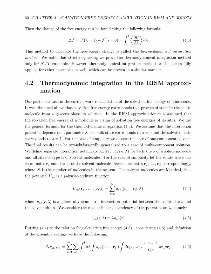
60 CHAPTER 4. SOLVATION FREE ENERGY CALCULATION IN RISM AND 3DRISM
Then the change of the free energy can be found using the following formula:
∆F = F(λ = 1)−F(λ = 0) =
∫ 1
0
⟨∂U
∂λ
⟩
dλ (4.3)
This method to calculate the free energy change is called the thermodynamical integration
method. We note, that strictly speaking we prove the thermodynamical integration method
only for NV T ensemble. However, thermodynamical integration method can be successfully
applied for other ensembles as well, which can be proven in a similar manner.
4.2 Thermodynamic integration in the RISM approxi-
mation
Our particular task in the current work is calculation of the solvation free energy of a molecule.
It was discussed above that solvation free energy corresponds to a process of transfer the solute
molecule from a gaseous phase to solution. In the RISM approximation it is assumed that
the solvation free energy of a molecule is a sum of solvation free energies of its sites. We use
the general formula for the thermodynamic integration (4.3). We assume that the interaction
potential depends on a parameter λ, the bulk state corresponds to λ = 0 and the solvated state
corresponds to λ = 1. For the sake of simplicity we discuss the case of one-component solvent.
The final results can be straightforwardly generalized to a case of multi-component solution.
We define separate interaction potentials Usα(r1, . . . , rN , λ) for each site s of a solute molecule
and all sites of type α of solvent molecules. For the sake of simplicity let the solute site s has
coordinates r1 and sites α of the solvent molecules have coordinates r2, . . . , rN correspondingly,
where N is the number of molecules in the system. The solvent molecules are identical, thus
the potential Usα is a pairwise-additive function:
Usα(r1, . . . , rN , λ) =N∑
j=2
usα(|rj − r1|, λ) (4.4)
where usα(r, λ) is a spherically symmetric interaction potential between the solute site s and
the solvent site α. We consider the case of linear dependency of the potential on λ, namely:
usα(r, λ) ≡ λusα(r) (4.5)
Putting (4.4) to the relation for calculating free energy (4.3) , considering (4.5) and definition
of the ensemble average we have the following:
∆FRISM =N∑
j=2
∑
sα
∫ 1
0
dλ
∫
usα(|rj − r1|)∫
dr1 . . . drNe−βUsα(λ)
QN
dr1drj (4.6)
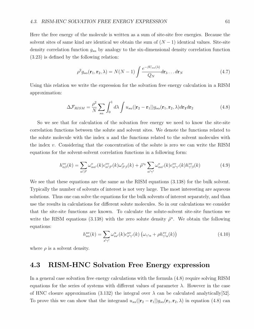
4.3. RISM-HNC SOLVATION FREE ENERGY EXPRESSION 61
Here the free energy of the molecule is written as a sum of site-site free energies. Because the
solvent sites of same kind are identical we obtain the sum of (N − 1) identical values. Site-site
density correlation function gsα by analogy to the six-dimensional density correlation function
(3.23) is defined by the following relation:
ρ2gsα(r1, r2, λ) = N(N − 1)
∫e−βUsα(λ)
QN
dr3 . . . drN (4.7)
Using this relation we write the expression for the solvation free energy calculation in a RISM
approximation:
∆FRISM =ρ2
N
∑
sα
∫ 1
0
dλ
∫
usα(|r2 − r1|)gsα(r1, r2, λ)dr1dr2 (4.8)
So we see that for calculation of the solvation free energy we need to know the site-site
correlation functions between the solute and solvent sites. We denote the functions related to
the solute molecule with the index u and the functions related to the solvent molecules with
the index v. Considering that the concentration of the solute is zero we can write the RISM
equations for the solvent-solvent correlation functions in a following form:
hvvαβ(k) =
∑
α′β′
ωvαα′(k)cvvα′β′(k)ωv
β′β(k) + ρvk∑
α′γ′
ωvαα′(k)cvvα′γ′(k)hvv
γ′β(k) (4.9)
We see that these equations are the same as the RISM equations (3.138) for the bulk solvent.
Typically the number of solvents of interest is not very large. The most interesting are aqueous
solutions. Thus one can solve the equations for the bulk solvents of interest separately, and than
use the results in calculations for different solute molecules. So in our calculations we consider
that the site-site functions are known. To calculate the solute-solvent site-site functions we
write the RISM equations (3.138) with the zero solute density ρu. We obtain the following
equations:
huvsα(k) =
∑
s′γ′
ωuss′(k)c
uvs′γ′(k)
(ωγ′α + ρhvv
γ′α(k))
(4.10)
where ρ is a solvent density.
4.3 RISM-HNC Solvation Free Energy expression
In a general case solvation free energy calculations with the formula (4.8) require solving RISM
equations for the series of systems with different values of parameter λ. However in the case
of HNC closure approximation (3.132) the integral over λ can be calculated analytically[52].
To prove this we can show that the integrand usα(|r2 − r1|)gsα(r1, r2, λ) in equation (4.8) can
62 CHAPTER 4. SOLVATION FREE ENERGY CALCULATION IN RISM AND 3DRISM
be represented as a full derivative over λ. By taking the derivative over λ of the HNC closure
(3.131) for usα(r;λ) = λusα(r) we obtain the following relation:
∂hsα(r, λ)
∂λ= e−βusα(r;λ)+hsα(r,λ)−csα(r,λ) ·
(
−βusα(r) +∂hsα(r, λ)
∂λ− ∂csα(r, λ)
∂λ
)
(4.11)
Putting the left hand side of the HNC closure to the right hand side of (4.11) and using that
gsα(r, λ) = hsα(r, λ) + 1 we come to the following expression:
∂hsα(r, λ)
∂λ= −βgsα(r, λ)usα(r) + (hsα(r, λ) + 1)
∂
∂λ(hsα(r, λ)− csα(r, λ)) (4.12)
After opening the brackets in the right hand side of this expression we obtain the following:
∂hsα(r, λ)
∂λ= −βgsα(r, λ)usα(r) + hsα(r, λ)
∂hsα(r, λ)
∂λ+
∂hsα(r, λ)
∂λ− h
∂csα(r, λ)
∂λ− ∂csα(r, λ)
∂λ(4.13)
Canceling ∂h∂λ
and using the relation h∂h∂λ
= ∂∂λ(h
2
2) we have the following:
gsα(r, λ)usα(r) =1
β
(∂
∂λ
(h2sα(r, λ)
2− csα(r, λ)
)
− hsα(r, λ)∂csα(r, λ)
∂λ
)
(4.14)
Putting it to the expression (4.8) and using that β = 1kBT
we have the following:
∆FHNC =ρ2
N
∑
sα
∫ (h2sα(r)
2− csα(r)
)
dr1dr2−∑
sα
∫
dr1dr2
∫ 1
0
dλhsα(r, λ)∂csα(r, λ)
∂λ(4.15)
where hsα(r, λ = 1) ≡ hsα(r), csα(r, λ = 1) ≡ csα(r) and hsα(r, λ = 0) = csα(r, λ = 0) = 0.
The first summand in (4.15) is already expressed without the integration over λ. To avoid
the integration over λ in the second summand we use the integration by parts method and
obtain the following relation:
∑
sα
∫
dr1dr2
∫ 1
0
dλhsα(r, λ)∂csα(r, λ)
∂λ=
∑
sα
(∫
dr1dr2hsα(r)csα(r)−∫
dr1dr2
∫ 1
0
dλcsα(r, λ)∂hsα(r, λ)
∂λ
) (4.16)
Let us show that the following equality holds:
∑
sα
∫
dr1dr2hsα(r, λ)∂csα(r, λ)
∂λ=∑
sα
∫
dr1dr2csα(r, λ)∂hsα(r, λ)
∂λ(4.17)
To do this we use the RISM equations (4.10) in a real-space representation, namely:
hsα(|r2 − r1|, λ) =∑
s′α′
∫
ωss′(|r1 − r′|)cs′α′(|r′ − r′′|, λ)χα′α(|r′′ − r2|)dr′dr′′ (4.18)
4.3. RISM-HNC SOLVATION FREE ENERGY EXPRESSION 63
Using the equation (4.18) we find the left and right hand sides of (4.17) . The left hand side
can be expressed in a following way:
∑
sα
∫
dr1dr2hsα(r, λ)∂csα(r, λ)
∂λ=
∑
sα
∑
s′α′
∫
dr1dr2dr′dr′′ωss′(|r1 − r′|)cs′α′(|r′ − r′′|, λ)χα′α(|r′′ − r2|)
∂csα(|r1 − r2|, λ)∂λ
(4.19)
The right hand side has a following representation:
∑
sα
∫
dr1dr2csα(r, λ)∂hsα(r, λ)
∂λ=
∑
sα
∑
s′α′
∫
dr1dr2dr′dr′′csα(|r1 − r2|, λ)ωss′(|r1 − r′|)∂cs′α′(|r′ − r′′|, λ)
∂λχα′α(|r′′ − r2|) (4.20)
We can see that after renaming variables (r1 ↔ r′ ,r2 ↔ r′′ ) the right hand side of expression
(4.19) coincides with the right hand side of (4.20) In such a way the relation (4.17) is proved.
Putting it to expression (4.16) we have the following:
∑
sα
∫
dr1dr2
∫ 1
0
dλhsα(r, λ)∂csα(r, λ)
∂λ=
1
2
∑
sα
∫
dr1dr2hsα(r)csα(r) (4.21)
Putting (4.21) to (4.15) we obtain the following Solvation Free Energy expression for the HNC
approximation:
∆FHNC =ρ2
NkBT
∑
sα
∫
dr1dr2
(h2sα(r)
2− csα(r)−
1
2hsα(r)csα(r)
)
(4.22)
The functions hsα(r), csα(r) depend only on the relative displacement of molecule sites. Intro-
ducing the variable r = r2 − r1 we can avoid the double integration. The integral over r1 gives
the volume V . So, we obtain the following expression:
∆FHNC = ρkBT∑
sα
∫ (h2sα(r)
2− csα(r)−
1
2hsα(r)csα(r)
)
dr (4.23)
Using the spherical symmetry of the functions hsα(r), csα(r) the integral can be calculated as
a integral of the radial part (in spherical coordinates). So the final formula for calculation the
SFE in HNC approximation is the following:
∆FHNC = 4πρkBT∑
sα
∞∫
0
(h2sα(r)
2− csα(r)−
1
2hsα(r)csα(r)
)
r2dr (4.24)
64 CHAPTER 4. SOLVATION FREE ENERGY CALCULATION IN RISM AND 3DRISM
Doing the similar transformations for the KH closure (3.133) one can obtain the following
solvation free energy expression:
∆FKH = 4πρkBT∑
sα
∞∫
0
(h2sα(r)
2θ(−hsα(r))− csα(r)−
1
2hsα(r)csα(r)
)
r2dr (4.25)
where θ(r) is a Heaviside step function.
4.4 Other Solvation Free Energy Expressions
In spite that formulae (4.24) and (4.25) were obtained from the rigorous mathematical trans-
formations, they are quite inaccurate in practical applications[62]. Two main sources of errors
are the RISM approximations and assumption that the free energy of the molecule is a sum of
free energies of its sites. As it was mentioned above the main assumptions of the RISM theory
are:
1. The assumption, that the molecular direct correlation function c(r,θ) can be represented
as a sum of site-site functions (3.111).
2. The assumption, that the molecular closure relation (3.109) can be substituted by the set
of site-site closure relations (3.131)
3. The assumption, that the solvation free energy of a molecule is a sum of solvation free
energies of its sites.
The first assumption simply states, that the six-dimensional function can be reconstructed
from its site-site projections. It is true at the large distances (where c is proportional to the
potential). Of course, not any six-dimensional function is a sum of one-dimensional projections.
However, in most cases this assumption should not lead to large errors. The same is not true for
the second and third assumptions. These assumptions actually are equivalent to the assumption
that the sites of the solvent molecules do no interact to each other, which is not true. Although
RISM equations (3.130) are obtained by averaging of the six-dimensional OZ equation, the
RISM closure relation (3.131) cannot be obtained by averaging of the six-dimensional closure
relation, and thus contradicts it. The same situation is with the RISM SFE expressions. In
this section we will consider the RISM-HNC solvation free energy expression in more details.
In the previous section the HNC expression for RISM approximation was derived. Similarly
the HNC solvation free energy expression for the six-dimensional OZ equation can be derived.

4.4. OTHER SOLVATION FREE ENERGY EXPRESSIONS 65
The six-dimensional analogy of the expression (4.22) is written in a following way:
∆GHNC =ρ2
NΩ2
∫ (1
2(h(r1, r2,θ1,θ2))
2 − c(r1, r2,θ1,θ2)−1
2h(r1, r2,θ1,θ2)c(r1, r2,θ1,θ2)
)
dr1dr2dθ1dθ2
(4.26)
where Ω =∫dθ. For the sake of simplicity this expression can be written in a more compact
form:
∆GHNC =ρ2
N
(1
2X − Y − 1
2Z
)
(4.27)
where X = Ω−2∫(h(r1, r2,θ1,θ2))
2 dr1dr2dθ1dθ2, Y = Ω−2∫c(r1, r2,θ1,θ2)dr1dr2dθ1dθ2,
Z = Ω−2∫h(r1, r2,θ1,θ2)c(r1, r2,θ1,θ2)dr1dr2dθ1dθ2. We will use only the first RISM ap-
proximation (3.113) to obtain the proper SFE expression. Putting (3.113) to the second sum-
mand in (4.27) we get the following relation:
Y =∑
sα
∫ (1
Ω
∫
δ(r1 + dus (θ1)− r1)dr1dθ1
)(1
Ω
∫
δ(r2 + dvα(θ2)− r2)dr2dθ2
)
csα(r1, r2)dr1dr2
(4.28)
Considering that∫δ(r+dv
α(θ)− r)dr = 1,∫dθ = Ω, we get the following expression for Y :
Y =∑
sα
∫
csα(r1, r2)dr1dr2 (4.29)
Putting (3.113) to the third summand in (4.27) we get the following expression:
Z =∑
sα
∫ (1
Ω2
∫
δ(r1 + dus (θ1)− r1)δ(r2 + dv
α(θ2)− r2)h(r1, r2,θ1,θ2)dr1dr2dθ1dθ2
)
csα(r1, r2)dr1dr2
(4.30)
Using the definition of the site-site total correlation function (3.114) we get the following ex-
pression:
Z =∑
sα
∫
hsα(r1, r2)csα(r1, r2)dr1dr2 (4.31)
We note, that the expressions for the summands (4.29), (4.31) are the same as the expressions
for the second and third summand in the RISM-HNC solvation free energy expression (4.22).
Thus, this part of the RISM-HNC expression is consistent with the six-dimensional expression.
However, it is not so for the first summand. Indeed, the first summand does not contain c-
function, thus it could not be straightforwardly reduced to the site-site form. And it is not
equal the sum of the site-site summands:
X =
∫
(h(r1, r2,θ1,θ2))2 dr1dr2dθ1dθ2 6=
∑
sα
∫
h2sα(r)dr1dr2 (4.32)
66 CHAPTER 4. SOLVATION FREE ENERGY CALCULATION IN RISM AND 3DRISM
This is one of the main sources of the errors of the RISM-HNC and RISM-KH expression (4.24),
(4.25). For example, it was shown, that RISM-HNC solvation free energy grows linearly with
the number of sites in the molecule, even if the sites are artificially introduced and have the
same coordinates [111]. Such a behavior is unphysical.
There were proposed several other SFE formulae which try to correct the errors of the
RISM-HNC solvation free energy approximations. In Ref. [112] the sources of the errors were
analyzed and it was pointed out that the HNC model typically overestimates the hydrogen bond
contribution to the solvation free energy. In that work it was proposed to introduce additional
correction to the SFE expression which contains the additional repulsing potential. This model
is typically called HNC with the repulsive bridge correction (HNCB). The solvation free energy
in the HNCB model is calculated using the following formula:
∆FHNCB = ∆FHNC + 4πρkBT∑
sα
(hsα(r) + 1)(e−bRsα(r) − 1)r2dr (4.33)
where bRsα(r) is defined with the following relation:
e−bRsα(|r|) =∏
β 6=α
∫
V
ωαβ(|r′ − r|) exp(
−βǫsβ
(σsβ
|r|
)12)
dr′ (4.34)
where σsβ, ǫsβ are pair Lennard-Jones parameters of the solute-solvent site-site potential.
Another approximation is Gaussian Fluctuations, (GF) formula which was initially proposed
in Ref. [113].
∆FGF = 4πρkBT∑
sα
∞∫
0
(
−csα(r)−1
2hsα(r)csα(r)
)
r2dr (4.35)
We see, that this formula simply neglects the first summand (h2/2) of the RISM-HNC expres-
sion, and in such a way avoids the linear dependency of the solvation free energy on the number
of sites in the molecule. However, neglecting of the “problematic” summand can also introduce
additional errors.
More elegant way was proposed in Ref. [62] by Ten-no et al. In this work the first summand
in the six-dimensional HNC expression is approximated using the Partial Wave (PW) method.
In the partial wave method the expression for the solvation free energy calculation has the
following form:
∆FPW = ∆FGF + 2πρkBT∑
sα
∫ ∞
0
hsα(r)hsα(r)r2dr (4.36)
where the Fourier transform of the functions hsα(r) is defined in a following way:
hsα(k) =∑
s′α′
ωuss′(k)hsα(k)ω
vα′α(k) (4.37)
4.5. SEMI-EMPIRICAL SOLVATION FREE ENERGY EXPRESSIONS 67
where ωuss′(k), ω
vα′α(k) are the elements of matrices which are inverse to the matrices of in-
tramolecular functions Wu and Wv (3.169). It was shown that the PW expression is more
suitable for the SFE calculations than KH and GF expressions [65].
4.5 Semi-Empirical methods for RISM Solvation Free
Energy calculation
As it was discussed above, advanced RISM solvation free energy expressions can correct some
systematic errors of the RISM calculations. Nevertheless, accuracy of these methods still often
appears to be too low for the practical applications. That’s why semi-empirical approaches are
used for the accurate SFE calculations with RISM and 3DRISM. One of the way to develop
the semi-empirical SFE calculation method is to parameterize the difference between the ex-
perimentally measured SFE ∆Gexp and the value ∆GRISM calculated with one of the RISM
SFE expressions. To parameterize this difference one can use some known parameters of the
molecule (descriptors). The most straightforward is the linear parameterization model where
the error is assumed to be linearly proportional to the descriptors. Let D1, . . . , DM be the
descriptors. Then the linear parameterization model can be written as follows:
ε = ∆Gexp −∆GRISM =M∑
i=1
aiDi (4.38)
where a1, . . . , aM are the free coefficients. The free coefficients a1, . . . , aM can be calculated
using the least squares method. To calculate them the training set of compounds should be
chosen. It is assumed that for this set of compounds experimentally measured SFEs and the
values of all descriptors D1, . . . , DM are known. Let ∆GkRISM , ∆Gk
exp be the calculated and the
experimentally measured SFEs of the kth molecule in the training set. Let Dk1 , . . . , D
kM be the
descriptors of the kth molecule in the training set. Using the linear model (4.38) we can write
the following approximate relations for all the molecules in the training set:
εk = ∆Gkexp −∆Gk
RISM ≈M∑
i=1
aiDki (4.39)
Following the least squares method the coefficients a1, . . . , aM should be chosen in the way that
minimizes the following expression:
N∑
k=1
(
εk −M∑
i=1
aiDki
)2
→ min (4.40)
where N is the number of the molecules in the training set. Using the matrix representation
we can rewrite this expression in a following way:
(ε−Da)T (ε−Da) → min (4.41)

68 CHAPTER 4. SOLVATION FREE ENERGY CALCULATION IN RISM AND 3DRISM
where ε = (ε1, . . . , εN)T , D = [Dk
i ]N×M , a = (a1, . . . , aM)T . The necessary condition of the
minimum is equality of the partial derivatives over the all parameters a1, . . . , aM to zero. We
obtain the following relation:
N∑
k=1
(εk −M∑
i=1
aiDki ) ·Dk
j = 0
j = 1 . . .M
(4.42)
This relation in a matrix form can be written in a following way:
(ε−Da)T D = 0 (4.43)
From this relation the free coefficients a can be expressed in a following form:
aT = εTD(DTD
)−1(4.44)
After calculating of the free coefficients the formula for the semi-empirical SFE calculations is
determined. It reads as follows:
∆Gcorr = ∆GRISM +M∑
i=1
aiDi (4.45)
To check accuracy of this expression one need to perform SFE calculations on the test set
of compounds and compare results to the experimental ones. The test and the training sets
of compounds should not overlap. To check how good is the semi-empirical expression the
following quantities can be calculated on the test set of compounds:
• Correlation coefficient between the experimental and calculated values.
• Mean deviation MD(∆Gcorr,∆Gexp) :
MD(∆Gcorr,∆Gexp) =
N1∑
k=1
(∆Gk
corr −∆Gkexp
)
• Root Mean Squared Deviation (RMSD):
RMSD(∆Gcorr,∆Gexp) =
√√√√ 1
N1
N1∑
k=1
(∆Gk
corr −∆Gkexp
)2
• Standard Deviation (SD):
SD(∆Gcorr,∆Gexp) =√
RMSD(∆Gcorr,∆Gexp)2 −MD(∆Gcorr,∆Gexp)2
where N1 is the number of compounds in the training set.
4.6. MODELS BASED ON THE PARTIAL MOLAR VOLUME CORRECTION 69
4.6 Semi-empirical models based on the partial molar
volume correction
Predictability of a semi-empirical model strongly depends on the choice of descriptors. The
descriptors used in the model should met the following requirements:
• The values of the descriptors should be known or simply computable for any molecule to
which the model is applicable.
• The values of the descriptors should correlate with the errors of the RISM SFE expression
used in calculations (otherwise these descriptors are not useful).
One of the perspective descriptors for the RISM SFE calculations is the Partial Molar Volume
(PMV) of the molecule. It was shown that the error of RISM expressions correlate with
PMV[37]. Also, PMV can be simply calculated from the site-site correlation functions in both:
RISM and 3DRISM theories[24]. In Ref. [37] it was proposed to parameterize RISM SFE
expressions with PMV and the number of OH-groups in the molecule. It was shown that using
this parameterization method it is possible to predict SFE of the limited number of small organic
molecules with the accuracy of about 1 kcal/mol. This approach was developed afterwards in
the Structural Descriptor Correction (SDC) method, which includes PMV descriptor and the
structural descriptors, e.g. number of double bonds in the molecule, number of branches,
number of specific groups etc. [65]. This method was tested on a large set of more than 100
organic compounds. It was shown that the method is able to predict SFE with the accuracy
of 1-1.2 kcal/mol. Later on the SDC method was used for the calculation of the SFE of the
pollutants[66]. It was shown that for this set of molecules the error of the SDC model is about
0.9 kcal/mol. In such a way the transferability of the method was proven.
Despite of the amazing results, there are some compounds for which the SDC method
is hardly applicable. To use the SDC method one needs to calculate first the values of all
descriptors. However, it can be non-trivial task for some complicated molecules, because often
there are more than one way to divide these molecules into the functional groups. For such
molecules the simplified atomic-type correction (ATC) can be applied. In the ATC model the
descriptors are PMV and the numbers of atoms of each type in the molecule [64]. Typically,
atomic type correction model gives worse results in comparison to the SDC model. However,
it can be applied to any kind of molecule of arbitrary complexity, while SDC is limited to the
molecules which could be simply divided into the molecular groups.
The PMV-based parameterization model was also proposed for 3DRISM. It was shown, that
using only two descriptors (PMV and shift) it is possible to predict SFE with the accuracy of
1 kcal/mol [109]. This model was called Universal Correction (UC) model. UC model for a

70 CHAPTER 4. SOLVATION FREE ENERGY CALCULATION IN RISM AND 3DRISM
different sets of organic and drug-like compounds and demonstrated quite good accuracy of
predictions [74].
In our work we use the ATC model for the RISM and the UC model for the 3DRISM SFE
calculations.

Chapter 5
RISM Multi-Grid algorithm for
Solvation Free Energy calculations
In this chapter the multi-grid algorithm for solving RISM equations is described. The applica-
bility of the algorithm to the solvation free energy calculation is checked by benchmarking on
the set of drug-like compounds. This chapter is based on Refs. [114] and [67].
5.1 RISM equations representation suitable for the nu-
merical solution
5.1.1 Indirect correlation functions
The RISM equations in form (3.138) are not suitable for the numerical solution. The main
causes are: 1) the site-site correlation functions decay slowly, and thus cannot be effectively
discretized, 2) the closure relation in a form (3.131) cannot be used to express c-functions due
to huge numerical errors. We will discuss below these problems in details and also give a more
suitable notation for RISM equation which can be used for the iterative solution. For the
sake of simplicity we discuss below the case of one component solvent. The equations can be
straightforwardly generalized to a case of for multi-component solvents as well. The following
functions are involved in the RISM equation for the infinitely diluted solution: (i) total and
direct site-site correlation functions hsα(r) and csα(r) describing correlations between the
site s of the solute molecule and sites α of the solvent molecules, (ii) intramolecular correla-
tion functions wss′(r) describing the structure of the solute molecule, and (iii) bulk solvent
susceptibility functions χαα′(r) describing the structure of the pure solvent. Assume that
the solute molecule has M sites and the solvent molecule has K sites. The RISM convolution
equation is easier to formulate in the Fourier space:
H = W · C · X, (5.1)
71
72 CHAPTER 5. RISM MULTI-GRID ALGORITHM
where the matrices H, C, W, X are defined as follows: H = [hsα(k)]M×K , C = [csα(k)]M×K ,
W = [wss′(k)]M×M , X = [χαα′(k)]K×K . Here the hat symbol (ˆ) denotes the Fourier trans-
formed function. The transformation of a spherically symmetric function f(r) is defined by the
Bessel-Fourier transform (3.147).
Intramolecular correlation functions in the Fourier space wss′(k) are found via the relation
wss′(k) = δss′ + (1− δss′)sin krss′
krss′, (5.2)
where δss′ is the Kronecker delta and rss′ is the distance between the sites s and s′ of the solute
molecule. Susceptibility functions of bulk solvent functions are defined as
χαα′(k) = wsolvαα′ (k) + ρhsolv
αα′ (k), (5.3)
where ρ is the density of the solvent and wsolvαα′ (k) and hsolv
αα′ (k) are intramolecular and total
correlation functions of the bulk solvent. In the current work we use previously calculated
water susceptibility functions [83], therefore we do not discuss these calculations here, and just
assume them to be known functions in (5.1). Equation (5.1) is completed by the following
closure relation:
hsα(r) + 1 = exp (−βusα(r) + hsα(r)− csα(r) + Bsα(r)) , (5.4)
where β = 1/kBT , kB is a Boltzmann constant, T is a temperature, usα(r) is the site-site
potential and Bsα(r) is a bridge function.
It was discussed above that generally the exact expression for the Bridge function is not
known. We use the Kovalenko-Hirata closure relation in our calculations [115]:
hsα(r) + 1 =
eΞsα(r), Ξsα(r) < 0,Ξsα(r) Ξsα(r) > 0,
(5.5)
where Ξsα(r) = −βusα(r)+hsα(r)− csα(r) appears in the argument of the exponential function
in (5.4).
Typical iteration scheme of solving RISM equations includes two phases on each iteration
step: 1) From the RISM equations (5.1) obtain hsα and 2) From the closure relation (5.4) obtain
csα functions which can when be put to the (5.1). After that the procedure can be repeated
from the phase 1. Both of the phases seem to be straightforward. If we express csα functions
from the closure relation (5.4) we come to the following relation:
csα(r) = ln(hsα(r) + 1) + βusα(r) + hsα(r) + Bsα(r) (5.6)
The functions hsα(r) are connected to the site-site radial distribution functions gsα(r) in a
following way:
hsα(r) = gsα(r)− 1 (5.7)
5.1. ITERATIVE REPRESENTATION OF RISM EQUATIONS 73
Obviously two molecules cannot be simultaneously in the same place. The site-site correlation
functions are proportional to the probability to find the sites at the separation r there is some
radius r0 where with a good accuracy the following relations holds:
guvsα(r) = huvsα(r) + 1 = 0, r < r0 (5.8)
Putting (5.8) to (5.6) for the distances r < r0 we have to calculate the logarithm of zero. Of
cause, this is not exact zero, this is only almost a zero, because the probability to find one
particle inside the core of other one is non-zero. However nevertheless calculating logarithms
of so small numbers is numerically problematic and can cause an overflow or at least huge
numerical errors. To avoid these problems we define the indirect correlation functions γsα(r) =
hsα(r) − csα(r). Putting the expression for the indirect functions to the RISM equations we
obtain the following result:
γsα(k) =∑
s′α′
ωss′(k)cs′α′(k)χsolvα′α (k)− csα(k)
csα(r) = e−βusα(r)+γsα(r)+Bsα(r) − γsα(r)− 1s = 1 . . .M, α = 1 . . . K
(5.9)
Using equations in this form we can avoid taking the logarithm of the small values and associated
with it numerical problems.
5.1.2 RISM equations for short-range functions
Typically the direct correlation functions decay slow with a distance which can cause problems
with discretization of these functions. However, as it was discussed in the section 3.8 we know
asymptotic behavior of direct correlation functions, namely:
csα(r) = −βusα(r) (5.10)
For the charged particles the biggest contribution to the potential at the large distances is the
Coulomb interaction potential:1
usα(r) ≈qsqαr
r > r0 (5.11)
We introduce the short-range and long-range site-site potentials uSsα(r), u
Lsα(r) in a following
way:
uLsα(r) =
qsqαr
erf(τr) uSsα(r) = usα(r)− uL
sα(r) (5.12)
1 We use atomic units in our work to avoid scaling coefficients in the Coulomb interaction.

74 CHAPTER 5. RISM MULTI-GRID ALGORITHM
whereqsqαr
is a Coulomb potential, erf(r) = (2/√π)∫ r
0e−x2
dx is a Gauss error function, the
parameter τ determines the smoothness of the transition between the short-range and long-
range functions. The long-range direct correlation functions cLsα(r) are defined in a following
way:
cLsα(r) = −βuLsα(r) (5.13)
Short-range direct and indirect correlation functions cSsα(r) and γSsα(r) are defined as a difference
between the full and long range functions, namely:
cSsα(r) = csα(r)− cLsα(r) = csα(r) + βuLsα(r)
γSsα(r) = hsα(r)− cSsα(r) = γsα(r)− βuL
sα(r)(5.14)
Short-range functions are convenient for the numerical treatment of the task. They decay
rapidly with a distance and can be effectively approximated by the functions with a small
support. Putting the short-range functions to the closure relation we obtain the following
closure for the short-range functions:
cSsα(r) = e−βuSsα(r)−γS
sα(r)+Bsα(r) − γSsα(r)− 1 (5.15)
Following Ref. [116] we write the analytical representation of the Bessel-Fourier transform for
long-rang potential usα:
uLsα(k) =
4πqsqαk2
e−k2
4t2 (5.16)
We note that this function in the Fourier space is proportional to 1k2
and thus decays rapidly.
This enables us to use small-support grids in the Fourier space. Putting (5.14) to equation
(5.9) we obtain the following relations for the short-range functions:
γSsα(k) =
∑
s′ν
ωss′(k) ·(cSs′ν(k) + uL
sα(k))· (ωsolv
αν (k) + ρhsolvαν (k))− cSsα(k) (5.17)
5.1.3 RISM equations in a recurrent form
Equations (5.17), (5.15) can be represented in a matrix form. Let the solute and solvent
molecule have M and K sites correspondingly. We define the matrix of the short-range indirect
correlation functions Γ = [γSsα(r)]M×K and a matrix of the Fourier-transformed long range
potentials UL = [uLsα(k)]M×K in a following way:
Γ =
γS11(r) . . . γS
1K(r)...
. . ....
γSM1(r) . . . γS
MK(r)
(5.18)
UL =
uL11(k) . . . uL
1K(k)...
. . ....
uLM1(k) . . . uL
MK(k)
(5.19)
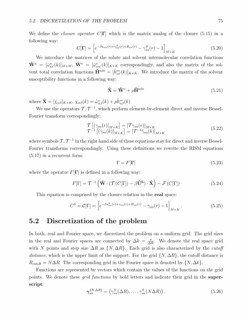
5.2. DISCRETIZATION OF THE PROBLEM 75
We define the closure operator C[Γ] which is the matrix analog of the closure (5.15) in a
following way:
C[Γ] =[
e−βusα(r)+γSsα(r)+Bsα(r) − γS
sα(r)− 1]
M×K(5.20)
We introduce the matrices of the solute and solvent intermolecular correlation functions
Wu = [ωuss′(k)]M×M , Wv = [ωv
αα′(k)]K×K correspondingly, and also the matrix of the sol-
vent total correlation functions Hsolv = [hvvss′(k)]K×K . We introduce the matrix of the solvent
susceptibility functions in a following way:
X = Wv + ρHsolv (5.21)
where X = [χαβ]K×K , χαβ(k) = ωvαβ(k) + ρhvv
αβ(k)
We use the operators T , T −1, which perform element-by-element direct and inverse Bessel-
Fourier transform correspondingly:
T[(γsα(r)]M×K
]= [T γsα(r)]M×K
T −1[(γsα(k)]M×K
]= [T −1γsα(k)]M×K
(5.22)
where symbols T , T −1 in the right hand side of these equations stay for direct and inverse Bessel-
Fourier transforms correspondingly. Using these definitions we rewrite the RISM equations
(5.17) in a recurrent form:
Γ = F [Γ] (5.23)
where the operator F [Γ] is defined in a following way:
F [Γ] = T −1(
W · (T (C[Γ])− βUL) · X)
−F (C[Γ]) (5.24)
This equation is comprised by the closure relation in the real space:
CS = C[Γ] =[
e−βuSsα(r)+γsα(r)+Bsα(r) − γsα(r)− 1
]
M×K. (5.25)
5.2 Discretization of the problem
In both, real and Fourier space, we discretized the problem on a uniform grid. The grid sizes
in the real and Fourier spaces are connected by ∆k = π∆R
. We denote the real space grid
with N points and step size ∆R as N,∆R. Each grid is also characterized by the cutoff
distance, which is the upper limit of the support. For the grid N,∆R, the cutoff distance is
Rcutoff = N∆R. The corresponding grid in the Fourier space is denoted by N,∆k.Functions are represented by vectors which contain the values of the functions on the grid
points. We denote these grid functions by bold letters and indicate their grid in the super-
script:
γN,∆Rsα =
(γSsα(∆R), . . . , γS
sα(N∆R)), (5.26)
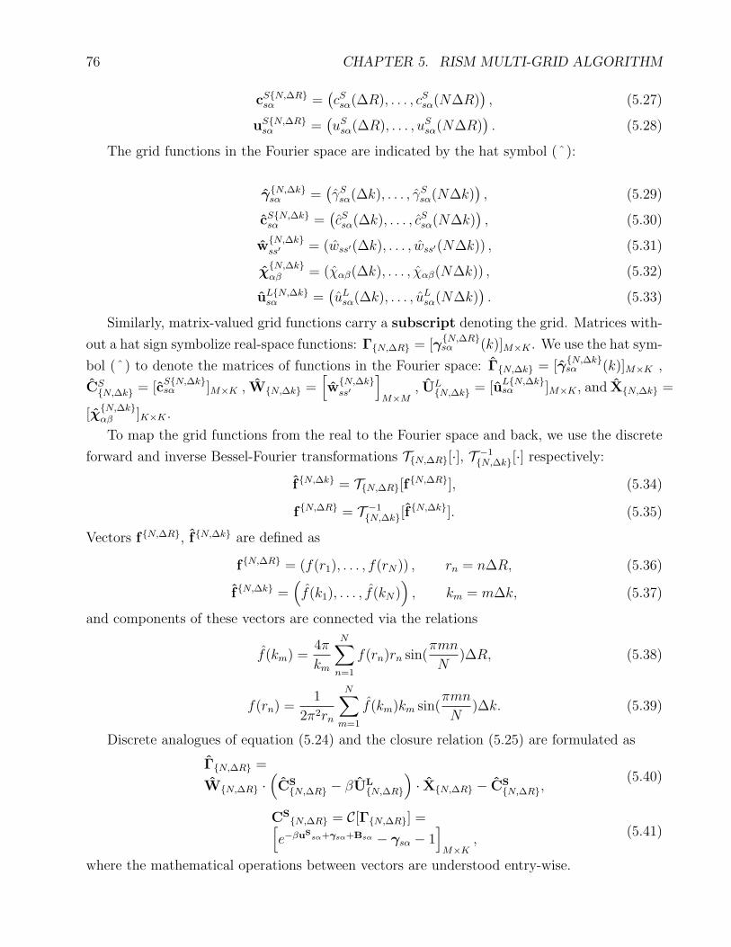
76 CHAPTER 5. RISM MULTI-GRID ALGORITHM
cSN,∆Rsα =
(cSsα(∆R), . . . , cSsα(N∆R)
), (5.27)
uSN,∆Rsα =
(uSsα(∆R), . . . , uS
sα(N∆R)). (5.28)
The grid functions in the Fourier space are indicated by the hat symbol (ˆ):
γN,∆ksα =
(γSsα(∆k), . . . , γS
sα(N∆k)), (5.29)
cSN,∆ksα =
(cSsα(∆k), . . . , cSsα(N∆k)
), (5.30)
wN,∆kss′ = (wss′(∆k), . . . , wss′(N∆k)) , (5.31)
χN,∆kαβ = (χαβ(∆k), . . . , χαβ(N∆k)) , (5.32)
uLN,∆ksα =
(uLsα(∆k), . . . , uL
sα(N∆k)). (5.33)
Similarly, matrix-valued grid functions carry a subscript denoting the grid. Matrices with-
out a hat sign symbolize real-space functions: ΓN,∆R = [γN,∆Rsα (k)]M×K . We use the hat sym-
bol (ˆ) to denote the matrices of functions in the Fourier space: ΓN,∆k = [γN,∆ksα (k)]M×K ,
CSN,∆k = [c
SN,∆ksα ]M×K , WN,∆k =
[
wN,∆kss′
]
M×M, UL
N,∆k = [uLN,∆ksα ]M×K , and XN,∆k =
[χN,∆kαβ ]K×K .
To map the grid functions from the real to the Fourier space and back, we use the discrete
forward and inverse Bessel-Fourier transformations TN,∆R[·], T −1N,∆k[·] respectively:
fN,∆k = TN,∆R[fN,∆R], (5.34)
fN,∆R = T −1N,∆k [f
N,∆k]. (5.35)
Vectors fN,∆R, fN,∆k are defined as
fN,∆R = (f(r1), . . . , f(rN)) , rn = n∆R, (5.36)
fN,∆k =(
f(k1), . . . , f(kN))
, km = m∆k, (5.37)
and components of these vectors are connected via the relations
f(km) =4π
km
N∑
n=1
f(rn)rn sin(πmn
N)∆R, (5.38)
f(rn) =1
2π2rn
N∑
m=1
f(km)km sin(πmn
N)∆k. (5.39)
Discrete analogues of equation (5.24) and the closure relation (5.25) are formulated as
ΓN,∆R =
WN,∆R ·(
CSN,∆R − βUL
N,∆R
)
· XN,∆R − CSN,∆R,
(5.40)
CSN,∆R = C[ΓN,∆R] =[
e−βuSsα+γsα+Bsα − γsα − 1
]
M×K,
(5.41)
where the mathematical operations between vectors are understood entry-wise.

5.3. PICARD ITERATION 77
5.3 Picard iteration
Combining (5.40) and(5.41) , we can define the iterative operator KN,∆R[·]:
KN,∆R[ΓN,∆R] ≡ T −1N,∆k
[
WN,∆k
(
TN,∆R[C[ΓN,∆R]
]− βUL
N,∆k
)
XN,∆k
−TN,∆R[C[ΓN,∆R]
]]
,
(5.42)
We consider the generalized task
ΓN,∆R = KN,∆R[ΓN,∆R] + fN,∆R (5.43)
for a given right-hand side vector fN,∆R. Problem (5.40) - (5.41) corresponds to the case
fN,∆R = 0. Necessity of introducing the generalized problem will be described bellow during
the description of the multi-grid method.
The n-th iterate of an iterative scheme is denoted by Γ(n)N,∆R. The damped Picard iteration
with the damping parameter λ is defined as
Γ(n+1)N,∆R = (1− λ)Γ
(n)N,∆R + λΓ′
N,∆R, (5.44)
where Γ′
N,∆R abbreviates
Γ′
N,∆R = KN,∆R[Γ(n)N,∆R] + fN,∆R. (5.45)
We use a short notation for this operator:
ΥN,∆R[Γ(n)N,∆R, fN,∆R]≡(1− λ)Γ
(n)N,∆R+ λΓ′
N,∆R. (5.46)
One iteration step of the algorithm consists of the partial steps
Γ(n)N,∆R
closure−−−−→(5.41)
CSN,∆R
BFT−−−→(5.34)
CSN,∆k
RISM−−−−→(5.40)
ΓN,∆kIBFT−−−→(5.35)
Γ′
N,∆Rdamping−−−−−→(5.44)
Γ(n+1)N,∆R.
(5.47)
As a measure of accuracy we use the L2 norm between two successive iterates averaged over
all site-site functions:∥∥∥Γ
(n+1)N,∆R − Γ
(n)N,∆R
∥∥∥ =
1
MK
∑
sα
√√√√
N∑
m=1
(γ(n+1)sα (m∆R)− γ(n)
sα (m∆R))2
∆R.(5.48)
We stop the iteration when the iterates differ by less than a given threshold ε :∥∥∥Γ
(n+1)N,∆R − Γ
(n)N,∆R
∥∥∥ ≤ ε. (5.49)

78 CHAPTER 5. RISM MULTI-GRID ALGORITHM
By n(N,∆R, ε) we denote the minimal number n such that (5.49) holds. So, using the
operator power notation, the iterative process to obtain the solution ΓεN,∆Rwith accuracy ε
can be written as
ΓεN,∆R =
(ΥN,∆R
)n(N,∆R,ε)[Γ
(0)N,∆R, fN,∆R]. (5.50)
5.4 Moving between the grids
In the multi-scale methods which we discuss below, several grids are used. Below we define
operators, which map grid functions from one grid to another: restriction operator r[·], inter-polation operator p[·] and extension operator e[·]
The restriction operator r[·] maps the matrix of grid functions to the coarser grid with
doubled grid size and, therefore, half the number of grid points. For example, the restriction
maps from the grid 2N,∆R to the grid N, 2∆R:
r[Γ2N,∆R] = ΓN,2∆R. (5.51)
In the current work we use the trivial injection as a restriction operator. Let Γ2N,∆R =
[γ2N,∆Rsα ]M×K , where
γ2N,∆Rsα = (γsα(∆R), γsα(2∆R) . . . , γsα(2N∆R)) (5.52)
and ΓN,2∆R = [γN,2∆Rsα ]M×K = r[Γ2N,∆R]. Then the vectors γ
N,2∆Rsα are defined by
γN,2∆Rsα = (γS
sα(2∆R), γSsα(4∆R), . . . , γS
sα(2N∆R)). (5.53)
We should mention that the restriction operator r[·] is linear:
r[aΓ′2N,∆R + bΓ′′
2N,∆R] =
a · r[Γ′2N,∆R] + b · r[Γ′′
2N,∆R].(5.54)
The interpolation operator p[·] maps the matrix of grid functions to the grid with half the
grid size and, thereby, the double number of grid points. For example, the interpolation maps
from the grid N, 2∆R to the grid 2N,∆R:
p[ΓN,2∆R] = Γ2N,∆R = [γ2N,∆Rsα ]. (5.55)
In the current work we use cubic spline interpolation as interpolation operator. Let ΓN,2∆R =
[γN,2∆Rsα ]M×K , where vectors γN,2∆R
sα are defined by (5.53) . Then γ2N,∆Rsα in (5.55) are
defined by
γ2N,∆Rsα = (γS
sα(∆R), γSsα(2∆R), γS
sα(3∆R), . . .. . . , γS
sα((2N − 1)∆R), γSsα(2N∆R)),
(5.56)

5.5. NESTED PICARD ITERATION 79
where the values γSsα((2k − 1)∆R) are obtained from the values γS
sα(2k∆R) using the cubic
spline interpolation.
We note that r[·] is the left-inverse of p[·], i.e., r[p[ΓN,2∆R]] = ΓN,2∆R, but not the
right-inverse:
Γ2N,∆R = p[r[Γ2N,∆R]] 6= Γ2N,∆R. (5.57)
However, sufficiently smooth functions satisfy
Γ2N,∆R = p[r[Γ2N,∆R]] = Γ2N,∆R +O(∆R). (5.58)
The extension operator e[·] does not change the grid size, but doubles the number of points.
For example, the extension maps from the grid N,∆R to the grid 2N,∆R:
e[ΓN,∆R] = Γ2N,∆R = [γ2N,∆Rsα ]M×K (5.59)
Indirect correlation functions decay fast to zero as the distance increases. Thus, it is natural to
extend them by zeros yielding the zero extension operator which we use in the current work.
Let ΓN,∆R = [γN,∆Rsα ]M×K with vectors γN,∆R
sα defined by (5.26). Then the functions
γ2N,∆Rsα in (5.59) are defined by
γ2N,∆Rsα = (γsα(∆R), . . . , γsα(N∆R), 0, . . . , 0
︸ ︷︷ ︸
N
). (5.60)
5.5 Nested Picard iteration
Independently of the convergence rate of an iterative scheme, the error of the n-th iterate
is the smaller the better the initial guess is. Having at hand different grids, the idea of the
nested Picard iteration [87] is straightforward: use as initial guess the (approximate) solution
from the coarse grid with a smaller number of grid points. Here we exploit that computations
in the coarse grid are cheaper. Below we describe the scheme of the nested Picard iteration.
Consider two grids: the “coarse” grid N, 2∆R and the “fine” grid 2N,∆R. We start from
the coarse-grid solution Γ(0)N,2∆R. We perform an iteration process of type (5.50) to obtain a
solution with accuracy ε on the coarse grid, interpolate it to the fine grid and use it as the
initial approximation for the fine-grid iteration.
The scheme for performing the two-grid nested Picard iteration is written as follows:
Γ(0)N,2∆R
ΥN,2∆R−−−−−→ ΓεN,2∆R
p−→→ Γ
(0)2N,∆R
Υ2N,∆R−−−−−→ Γε2N,∆R.
(5.61)
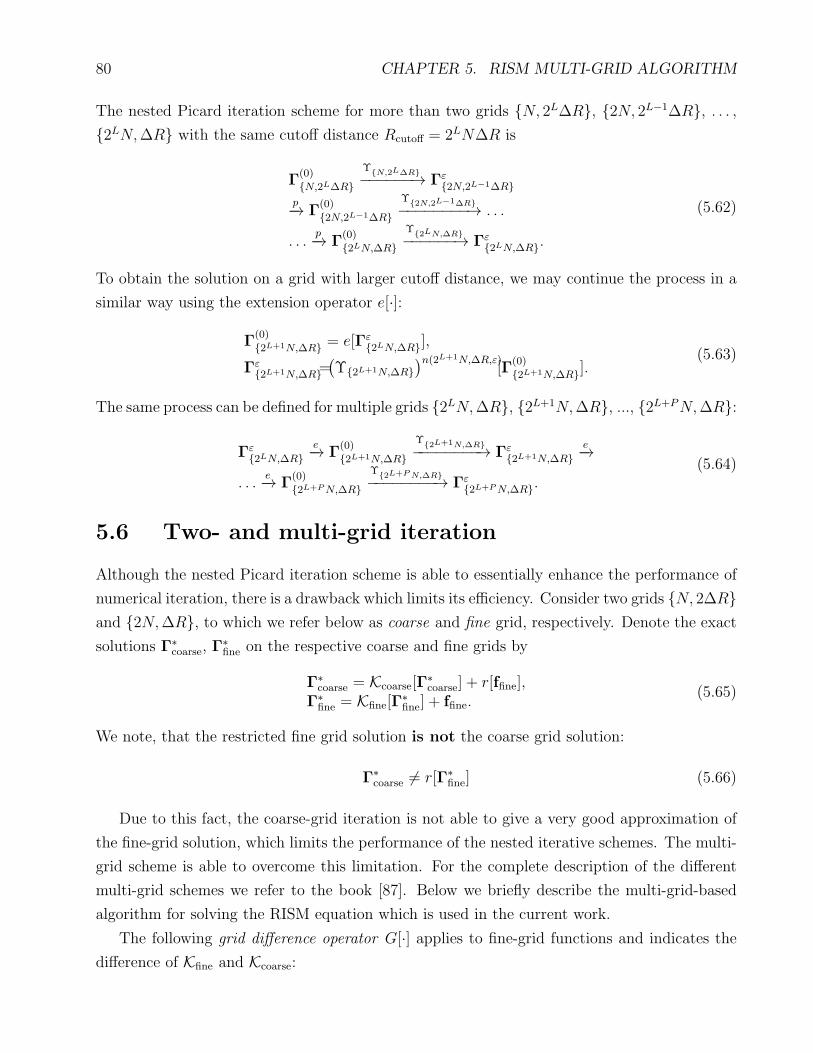
80 CHAPTER 5. RISM MULTI-GRID ALGORITHM
The nested Picard iteration scheme for more than two grids N, 2L∆R, 2N, 2L−1∆R, . . . ,2LN,∆R with the same cutoff distance Rcutoff = 2LN∆R is
Γ(0)
N,2L∆RΥ
N,2L∆R−−−−−−→ Γε2N,2L−1∆R
p−→ Γ(0)
2N,2L−1∆RΥ
2N,2L−1∆R−−−−−−−−→ . . .
. . .p−→ Γ
(0)
2LN,∆RΥ
2LN,∆R−−−−−−→ Γε2LN,∆R.
(5.62)
To obtain the solution on a grid with larger cutoff distance, we may continue the process in a
similar way using the extension operator e[·]:
Γ(0)
2L+1N,∆R = e[Γε2LN,∆R],
Γε2L+1N,∆R=
(Υ2L+1N,∆R
)n(2L+1N,∆R,ε)[Γ
(0)
2L+1N,∆R].(5.63)
The same process can be defined for multiple grids 2LN,∆R, 2L+1N,∆R, ..., 2L+PN,∆R:
Γε2LN,∆R
e−→ Γ(0)
2L+1N,∆RΥ
2L+1N,∆R−−−−−−−−→ Γε2L+1N,∆R
e−→
. . .e−→ Γ
(0)
2L+PN,∆RΥ
2L+PN,∆R−−−−−−−−→ Γε2L+PN,∆R.
(5.64)
5.6 Two- and multi-grid iteration
Although the nested Picard iteration scheme is able to essentially enhance the performance of
numerical iteration, there is a drawback which limits its efficiency. Consider two grids N, 2∆Rand 2N,∆R, to which we refer below as coarse and fine grid, respectively. Denote the exact
solutions Γ∗coarse, Γ
∗fine on the respective coarse and fine grids by
Γ∗coarse = Kcoarse[Γ
∗coarse] + r[ffine],
Γ∗fine = Kfine[Γ
∗fine] + ffine.
(5.65)
We note, that the restricted fine grid solution is not the coarse grid solution:
Γ∗coarse 6= r[Γ∗
fine] (5.66)
Due to this fact, the coarse-grid iteration is not able to give a very good approximation of
the fine-grid solution, which limits the performance of the nested iterative schemes. The multi-
grid scheme is able to overcome this limitation. For the complete description of the different
multi-grid schemes we refer to the book [87]. Below we briefly describe the multi-grid-based
algorithm for solving the RISM equation which is used in the current work.
The following grid difference operator G[·] applies to fine-grid functions and indicates the
difference of Kfine and Kcoarse:
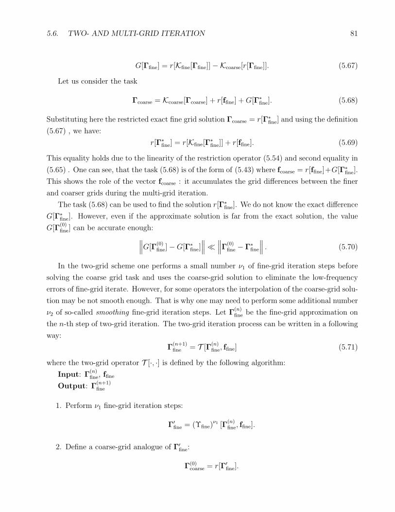
5.6. TWO- AND MULTI-GRID ITERATION 81
G[Γfine] = r[Kfine[Γfine]]−Kcoarse[r[Γfine]]. (5.67)
Let us consider the task
Γcoarse = Kcoarse[Γcoarse] + r[ffine] +G[Γ∗fine]. (5.68)
Substituting here the restricted exact fine grid solution Γcoarse = r[Γ∗fine] and using the definition
(5.67) , we have:
r[Γ∗fine] = r[Kfine[Γ
∗fine]] + r[ffine]. (5.69)
This equality holds due to the linearity of the restriction operator (5.54) and second equality in
(5.65) . One can see, that the task (5.68) is of the form of (5.43) where fcoarse = r[ffine]+G[Γ∗fine].
This shows the role of the vector fcoarse : it accumulates the grid differences between the finer
and coarser grids during the multi-grid iteration.
The task (5.68) can be used to find the solution r[Γ∗fine]. We do not know the exact difference
G[Γ∗fine]. However, even if the approximate solution is far from the exact solution, the value
G[Γ(0)fine] can be accurate enough:
∥∥∥G[Γ
(0)fine]−G[Γ∗
fine]∥∥∥≪
∥∥∥Γ
(0)fine − Γ∗
fine
∥∥∥ . (5.70)
In the two-grid scheme one performs a small number ν1 of fine-grid iteration steps before
solving the coarse grid task and uses the coarse-grid solution to eliminate the low-frequency
errors of fine-grid iterate. However, for some operators the interpolation of the coarse-grid solu-
tion may be not smooth enough. That is why one may need to perform some additional number
ν2 of so-called smoothing fine-grid iteration steps. Let Γ(n)fine be the fine-grid approximation on
the n-th step of two-grid iteration. The two-grid iteration process can be written in a following
way:
Γ(n+1)fine = T [Γ
(n)fine, ffine] (5.71)
where the two-grid operator T [·, ·] is defined by the following algorithm:
Input: Γ(n)fine, ffine
Output: Γ(n+1)fine
1. Perform ν1 fine-grid iteration steps:
Γ′fine = (Υfine)
ν1 [Γ(n)fine, ffine].
2. Define a coarse-grid analogue of Γ′fine:
Γ(0)coarse = r[Γ′
fine].
82 CHAPTER 5. RISM MULTI-GRID ALGORITHM
3. Calculate the grid correction G[Γ′fine]:
G[Γ′fine] = r[Kfine[Γ
′fine]]−Kcoarse[Γ
(0)coarse].
4. Determine the solution Γ∗coarse the coarse grid problem
Γcoarse = Kcoarse[Γcoarse] +G[Γ′fine] + r[ffine]. (5.72)
5. Add the coarse-grid correction:
Γ′′fine = Γ′
fine + p[Γ∗coarse − Γ(0)
coarse].
6. Perform ν2 smoothing fine-grid iteration steps:
Γ(n+1)fine = (Υfine)
ν2 [Γ′′fine, ffine].
In the two-grid algorithm it is not specified how the coarse-grid equation on the step 4 is
solved. If the same algorithm is used recursively for solving the coarse-grid problem, we obtain
the multi-grid iterative scheme [87]. Assume that we have the grids N, 2L∆R, 2N, 2L−1∆R,. . . , 2LN,∆R. We will use the subscript grid to refer to any of these grids. On each grid we
define the multi-grid iteration with iterative operator Mlevelgrid [Γ
(n)grid, fgrid]:
Γ(n+1)grid = Mlevel
grid [Γ(n)grid, fgrid], (5.73)
where Γ(n)grid is the n-th multi-grid iterate, fgrid is given, and the superscript level indicates the
number of recursions which are done while calculating the operator. The multi-grid iteration
converges to the solution of the task
Γgrid = Kgrid[Γgrid] + fgrid. (5.74)
The multi-grid operator at level zero is a single-grid solver of (5.74) on the coarsest grid.
In our work we use n steps of the damped Picard iteration:
M0N,2L∆R[Γ
(0)
N,2L∆R, fN,2L∆R] =(ΥN,2L∆R
)n[Γ
(0)
N,2L∆R, fN,2L∆R](5.75)
The proper choice of the number n of iteration steps on the coarsest grid is discussed in Section
5.8 . For the sake of brevity, below we use the subscript “fine” to refer to the grid 2ℓN, 2L−ℓ∆Rand the subscript “coarse” to refer to the grid 2ℓ−1N, 2L−ℓ+1∆R. The multi-grid operator
Mℓfine[Γ
(n)fine, ffine] of level ℓ > 0 is defined by the following algorithm:
Input: Γ(n)fine, ffine, ℓ
Output: Γ(n+1)fine

5.6. TWO- AND MULTI-GRID ITERATION 83
1. Perform ν1 steps of the fine-grid Picard iteration:
Γ′fine = (Υfine)
ν1 [Γ(n)fine, ffine].
2. Define a coarse-grid analogue of Γ′fine and use it as starting guess of the iteration in Step
4:
Γ(0)coarse = r[Γ′
fine].
3. Calculate grid correction G[Γ′fine]:
G[Γ′fine] = r[Kfine[Γ
′fine]]−Kcoarse[Γ
(0)coarse].
4. Perform, recursively, µ steps of the coarse-grid multi-grid iteration of level (ℓ− 1):
Γ(µ)coarse =
(Mℓ−1
coarse
)µ[Γ(0)
coarse, r[ffine] +G[Γ′fine]].
5. Add the coarse-grid correction:
Γ′′fine = Γ′
fine + p[Γ(µ)coarse − Γ(0)
coarse].
6. Perform ν2 steps of the fine-grid Picard iteration:
Γ(n+1)fine = (Υfine)
ν2 [Γ′′fine, ffine].
If in Step 4 the number of the multi-grid iteration steps is µ = 1, the multi-grid iteration is
called V-cycle. If µ = 2, the iteration is called W-cycle [87]. In the current work we use µ = 1.
In our case the iterative operator K[·] is smooth enough, thus for the multi-grid iteration we
use ν1 = 1 and ν2 = 0 on the steps 1, 6 of the algorithm, which is standard for the multi-grid
of the second kind [87].
Now we assume that grids with different cutoff distances are given: 2LN,∆R, 2L+1N,∆R,. . . , 2L+PN,∆R. We can use a scheme similar to (5.64) for the multi-grid iteration: having
solved the task on the grid 2LN,∆R by the multi-grid iteration up to accuracy ε, extend the
solution to the grid 2L+1N,∆R and use it as initial guess for a next multi-grid iteration and
so on. We denote by Γ(0)grid the initial approximation on the grid grid and by Γε
grid the solution
with the L2-norm accuracy ε, obtained via the iterative process (5.73) . The multi-grid iteration
with the grid extension can be written schematically as follows:
Γ(0)
2LN,∆R
ML
2LN,∆R−−−−−−−→ Γε2LN,∆R
e−→
Γ(0)
2L+1N,∆R
ML
2L+1N,∆R−−−−−−−−→ . . .
. . .e−→ Γ
(0)
2L+PN,∆R
ML
2L+PN,∆R−−−−−−−−→ Γε2L+PN,∆R.
(5.76)
84 CHAPTER 5. RISM MULTI-GRID ALGORITHM
5.7 Nested multi-grid
In any iteration the error of the n-th iterate is the smaller, the better the initial guess is. The
nested iteration technique suggests to use an approximate coarse-grid solution as initial guess
for the fine-grid iteration. In the multi-grid iteration the fine-grid initial guess can be found
via the multi-grid iteration on the coarser grid. Typically, it is enough to perform a single
multi-grid iteration on the coarser grid to obtain a good initial guess for the fine-grid iteration.
Assume grids N, 2L∆R, 2N, 2L−1∆R, . . . , 2LN,∆R and an initial guess Γ(0)
N,2L∆R on
the coarsest grid are given. We find an initial guess Γ(0)
2LN,∆R on the fine grid 2LN,∆R by
the following algorithm:
Input: Γ(0)
N,2L∆R
Output: Γ(0)
2LN,∆R
for ℓ=0. . .L-1:
1. Perform one multi-grid iteration on the coarse grid:
Γ(1)
2ℓN,2L−ℓ∆R = Mℓ2ℓN,2L−ℓ∆R(Γ
(0)
2ℓN,2L−ℓ∆R)
2. Interpolate the result to the finer grid:
Γ(0)
2ℓ+1N,2L−ℓ−1∆R = p[Γ(1)
2ℓN,2L−ℓ∆R]
The same can be written schematically:
Γ(0)
N,2L∆R
M0N,2L∆R−−−−−−−→ Γ
(1)
N,2L∆Rp−→
Γ(0)
2N,2L−1∆R
M12N,2L−1∆R−−−−−−−−−→ . . .
. . .ML−1
N,2L∆R−−−−−−−→ Γ(1)
2L−1N,2∆Rp−→
Γ(0)
2LN,∆R
(5.77)
Having the initial guess Γ(0)
2LN,∆R one can use the multi-grid iteration process (5.73) to
obtain the approximate solution on the grid 2LN,∆R with a given accuracy ε. After that,
using scheme (5.76) , one may extend the solution to the grid 2L+PN,∆R. In the current
paper we call the process (5.77) - (5.73)- (5.76) the nested multi-grid iteration, and compare its
performance to the multi-grid iteration (5.73) - (5.76) , to the nested Picard iteration (5.62)-
(5.64) , and to the one-level Picard iteration (5.47).

5.8. OPTIMAL NUMBER OF COARSE-GRID STEPS 85
5.8 Determining the optimal number of coarse-grid it-
eration steps
In the multi-grid algorithm on the coarsest grid we solve the task of type (5.72) with correction
G[Γ′fine]. Because G[Γ′
fine] is only an approximation of the G[Γ∗fine] there is no need to solve this
task with accuracy better than the accuracy εG[Γ′fine]
of calculation of G[Γ′fine], which is defined
as follows:
εG[Γ′fine]
= ‖G[Γ′fine]−G[Γ∗
fine]‖ . (5.78)
The value of εG[Γ′fine]
can be estimated using the expression
εG[Γ′fine]
≈∥∥∥G[Γ′
fine]−G[Γ(n+1)fine ]
∥∥∥ (5.79)
Let us assume that the error ε(n) of the solution decays exponentially with the number n
of the coarse-grid iteration steps:
ε(n) =∥∥Γ(n)
coarse − Γ∗coarse
∥∥ = ε(0) · δn (5.80)
The value of δ can be found to be
δ =ε(1)
ε(0)(5.81)
We may estimate ε(1) and ε(0) by the expressions
ε(1) ≈∥∥∥Γ
(1)coarse − Γ
(n)coarse
∥∥∥ ,
ε(0) ≈∥∥∥Γ
(0)coarse − Γ
(n)coarse
∥∥∥ .
(5.82)
For the optimal number nopt of iteration steps we obtain
ε(nopt) = ε(0) · δnopt = εG[Γ′fine]
(5.83)
Let the actual number of the iteration steps be n.
Dividing (5.80) by (5.83) we get
ε(n)
εG[Γ′]
=ε(0)δn
εG[Γ′]
= δn−nopt (5.84)
and find the optimal number of iteration steps as
nopt = logδεG[Γ′]
ε(0)(5.85)
where δ, εG[Γ′], ε(0) are estimated through (5.81), (5.79), (5.82) , respectively. So after each
multi-grid iteration step we may estimate the optimal number of iteration steps on the coarsest

86 CHAPTER 5. RISM MULTI-GRID ALGORITHM
grid and use this number in the next multi-grid iteration step. To avoid fast change of n from
one multi-grid iteration step to another, we start from some number n(0) of coarse-grid iteration
steps and use a damped iteration process for the number n(k) of the coarsest-grid iteration steps
on the k-th multi-grid iteration step:
n(k+1) = αn(k) + (1− α)nopt (5.86)
where 0 < α < 1 is the damping parameter.
5.9 Choice of optimal grid parameters for Hydration
Free Energy calculations
In the sections above we explained how to solve the RISM equations (5.40) - (5.41) numeri-
cally. During the numerical solution we perform iteration steps on several grids with different
grid sizes and cutoff distances. In principle, we are free to choose the parameters of the iter-
ations. However, we plan to apply the RISM for calculations of the Hydration Free Energy
(HFE). Thus, we would like to choose parameters which yield HFE values with given numerical
accuracy at minimal computational cost. HFE can be calculated using the Kirkwood’s ther-
modynamic integration formula [110]. In the RISM approximation, the HFE of a molecule is
found as the sum of the partial HFEs of the sites. In the scope of the HNC approximation,
the thermodynamic integration can be performed analytically and HFE (∆G) may be found
explicitly from the solutions of the RISM equation [52]:
∆GHNC =
2πρkT∑
sα
∞∫
0
[−2csα(r) + γsα(r) (csα(r) + γsα(r))] r2dr
(5.87)
where ρ is the bulk number density, k is the Boltzmann constant and T is the temperature.
Usually, HFE is measured in kilo-calories per mole (kcal/mol). The accuracy of experimental
HFE measurements for bioactive compounds is & 0.1 kcal/mol [93]. To make some theoretical
and statistical investigations, we typically need to obtain a computational accuracy of about 100
times higher than the experimental one. That means that we should choose the grid parameters
which allow us to calculate the expression (5.87) with accuracy of at least 0.001 kcal/mol. We
use a uniform grid which can be described by the grid size ∆R and cutoff distance Rcutoff . First,
we try to determine an appropriate grid size ∆R. We perform series of RISM calculations with
same cutoff distance and different grid sizes, and for each grid size we calculate the free energy
of solvation using (5.87) . We assume that the solution on the finest grid yields an almost exact
value of ∆GHNC . Let us denote by ∆G∆RHNC the HFE-value calculated on the grid with step

5.9. OPTIMAL PARAMETERS FOR CALCULATIONS 87
∆R, and by ∆GbestHNC the value of the HFE calculated on the finest grid. We can estimate the
error of the HFE calculations as difference of ∆G∆RHNC and the best value ∆Gbest
HNC :
Error(∆G∆RHNC) =
∣∣∆G∆R
HNC −∆GbestHNC
∣∣ (5.88)
In our calculations, we measure distances in atomic units (Bohr, 1 Bohr≈ 0.52 A) as they are
the most natural for the atomic scale. As the base grid size we choose ∆R0 = 0.1 Bohr, and then
make the solvation free energy calculations for the different grid sizes ∆R = ∆R0
2k, k = −3 . . . 6
(grid sizes from 0.8 Bohr to 1640
Bohr). The value of 1640
Bohr is taken to be an approximation
∆GbestHNC of the exact HFE-value. The cutoff distance is 204.8 Bohr. Calculations on all grids
are performed up to L2-norm accuracy ε = 10−10.
To find the optimal cutoff distance Rcutoff, we perform calculations with the fixed ∆R but
different Rcutoff . We estimate the error of HFE calculations by taking the integral in (5.87)
over the interval (Rcutoff,∞), because this is the part of the axis which we omit while using the
function with finite support:
Error(∆GHNC) =
2πρkT∑
sα
∞∫
Rcutoff
[−2csα(r) + γsα(r) (csα(r) + γsα(r))] r2dr (5.89)
To evaluate the infinite integral (5.89) , we can calculate functions γsα(r) and csα(r) on the grid
with a very large cutoff distance R∞cutoff and calculate the integral over the interval (Rcutoff,R
∞cutoff)
. As large cutoff distance we use R∞cutoff = 409.6 Bohr.
The most of computational time in the multi-grid iteration is spent on the coarsest grid.
The coarsest-grid solution should give a good approximation to the low-frequent part of the
exact solution. That means that using the coarsest-grid solution, we as well should be able
to roughly approximate chemical properties of the system, in particular the free energy of
hydration. HFE-values for a wide class of compounds lie in the range from -5 kcal/mol to +5
kcal/mol. That means that to obtain some qualitative information about the value of HFE
we need to have an accuracy in the calculations of at least 1-2 kcal/mol. In the current work
grid size and cutoff distance of the coarsest grid are chosen to give the numerical error in HFE
calculations ≤1 kcal/mol.
It is known that the solution of the RISM equations behave differently for neutral and
charged systems. That is why for determining the optimal grid parameters we have chosen five
different systems: single uncharged atom (Argon), simple charged ion pair (Sodium chloride),
uncharged molecule (methane), polar molecule with high partial charges of atoms (methanol)
and water.
We can find how much faster are nested Picard iteration, multi-grid and nested multi-grid
than the one-grid Picard iteration. To do the comparison we use the speed-up factors:

88 CHAPTER 5. RISM MULTI-GRID ALGORITHM
1/400.050.10.20.40.81.6
10−5
10−4
10−3
10−2
10−1
100
101
∆ R (Bohr)
Err
or o
f ∆ G
HN
C (
kcal
/mol
)
Desired coarsegrid accuracy
Desired fine−gridaccuracy
NaClArmethanemethanolwater
Figure 5.1: Dependencies of the error in hydration free energy calculations on the grid step ∆R(logarithmic scale). Calculations are done for the cutoff distance Rcutoff=204.8 Bohr.
SNMG(ε) =tone−grid(ε)
tNMG(ε)(5.90)
SMG(ε) =tone−grid(ε)
tMG(ε)(5.91)
SNest(ε) =tone−grid(ε)
tNP(ε)(5.92)
where tNMG(ε), tMG(ε), tNP(ε), tone−grid(ε) are the computer times to solve the RISM equa-
tions by the nested multi-grid method, multi-grid method, nested Picard iteration method
and one-level Picard iteration method up to the L2-norm accuracy ε respectively. The values
tNP(ε)/tMG(ε) and tNP(ε)/tNMG(ε) show how many times faster are the multi-grid and nested
multi-grid methods than the nested Picard iteration respectively.
5.10 Optimal grid parameters
To determine the appropriate grid parameters, the RISM Hydration Free Energy calculations
were performed for grids with different fine-grid sizes and different cutoff distances. One can
find details of calculation in the supporting information of the paper. In Figure 5.1 one can
see how the error of HFE calculations depends on the grid size. For all investigated systems

5.11. THE RISM-MOL SOLVER 89
12.8 25.6 51.2 102.4 204.810
−5
10−4
10−3
10−2
10−1
100
Rcutoff
(Bohr)
Err
or o
f ∆ G
HN
C (
kcal
/mol
)
Desired coarsegrid accuracy
Desired fine−gridaccuracy
NaClArmethanemethanolwater
Figure 5.2: Dependencies of the error in hydration free energy calculations on the cutoff distanceRcutoff (logarithmic scale).
starting from the grid size ∆R = 0.05 Bohr, the error is smaller than the desired threshold
0.001 kcal/mol. We take the grid with ∆R = 0.05 Bohr as the fine-grid for the numerical
solution of the RISM equations. To determine the optimal cutoff distance, we performed the
RISM calculations for the systems with very large cutoff distance R∞cutoff = 409.6 Bohr and
calculated the numerical error of HFE calculations with (5.89) for argon, sodium chloride,
methane, methanol and water. We use grids with 2p (p = 8 . . . 13) points which gives cutoff
distances from 12.8 Bohr to 409.6 Bohr. The results of the calculations are presented in Figure
5.2. We can see that to achieve the desired accuracy of HFE calculations one should use a
cutoff distance 204.8 Bohr, which corresponds to 4096 grid points with the grid size 0.05 Bohr.
Also, from Figures 5.1 and 5.2 one can see that a grid with ∆Rcoarse=0.8 Bohr, Rcoarsecutoff=25.6
Bohr is enough to give a numerical error in the HFE calculations less than 1 kcal/mol. Thus,
this grid size and cutoff distance are used in the current work as parameters of the coarsest-grid
in the multi-grid algorithm.
5.11 The RISM-MOL solver
In the current work the calculations of the RISM solute-solvent correlation functions were per-
formed with the RISM-MOL program package for fast solution of the RISM integral equations
developed by Maxim V. Fedorov and Volodymyr P. Sergiievskyi in the Computational Physical

90 CHAPTER 5. RISM MULTI-GRID ALGORITHM
10−10
10−8
10−6
10−4
0
5
10
15
20
25
30
35
40
45
L2−norm accuracy
spee
dup
(ton
e−le
vel/t m
etho
d)
4.5
27.2
31.3
Nested Picard
multi−grid
Nested multi−grid
Figure 5.3: Dependencies of the nested multi-grid speedup SNMG(ε) = tone−grid(ε)/tNMG(ε),the multi-grid speedup SMG(ε) = tone−grid(ε)/tMG(ε) and the nested Picard iteration speedupSNP(ε) = tone−grid(ε)/tNP(ε) on the L2-norm accuracy of calculations.
10−10
10−8
10−6
10−4
0
1
2
3
4
5
6
7
8
L2−norm accuracy
spee
dup:
t Nes
t/t MG
6.0
6.9multi−gridNested multi−grid
Figure 5.4: Dependencies of the nested multi-grid and multi-grid speedup with regards to thenested Picard iterations (tNP(ε)/tNMG(ε), tNP(ε)/tMG(ε)) on the L2-norm accuracy of calcula-tions.
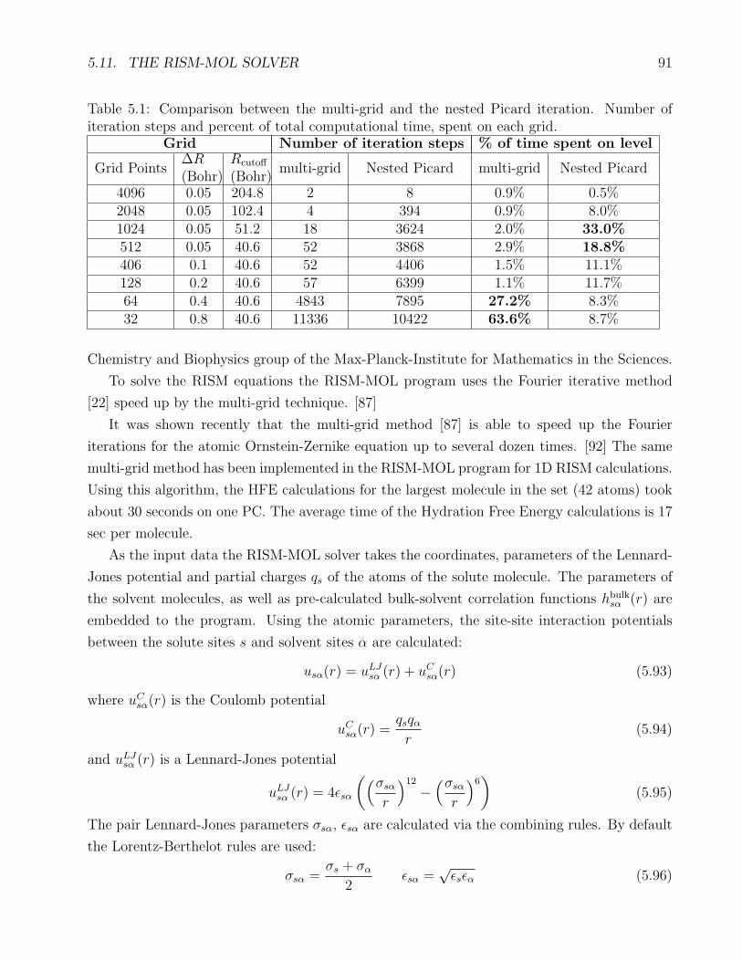
5.11. THE RISM-MOL SOLVER 91
Table 5.1: Comparison between the multi-grid and the nested Picard iteration. Number ofiteration steps and percent of total computational time, spent on each grid.
Grid Number of iteration steps % of time spent on level
Grid Points∆R(Bohr)
Rcutoff
(Bohr)multi-grid Nested Picard multi-grid Nested Picard
4096 0.05 204.8 2 8 0.9% 0.5%2048 0.05 102.4 4 394 0.9% 8.0%1024 0.05 51.2 18 3624 2.0% 33.0%
512 0.05 40.6 52 3868 2.9% 18.8%
406 0.1 40.6 52 4406 1.5% 11.1%128 0.2 40.6 57 6399 1.1% 11.7%64 0.4 40.6 4843 7895 27.2% 8.3%32 0.8 40.6 11336 10422 63.6% 8.7%
Chemistry and Biophysics group of the Max-Planck-Institute for Mathematics in the Sciences.
To solve the RISM equations the RISM-MOL program uses the Fourier iterative method
[22] speed up by the multi-grid technique. [87]
It was shown recently that the multi-grid method [87] is able to speed up the Fourier
iterations for the atomic Ornstein-Zernike equation up to several dozen times. [92] The same
multi-grid method has been implemented in the RISM-MOL program for 1D RISM calculations.
Using this algorithm, the HFE calculations for the largest molecule in the set (42 atoms) took
about 30 seconds on one PC. The average time of the Hydration Free Energy calculations is 17
sec per molecule.
As the input data the RISM-MOL solver takes the coordinates, parameters of the Lennard-
Jones potential and partial charges qs of the atoms of the solute molecule. The parameters of
the solvent molecules, as well as pre-calculated bulk-solvent correlation functions hbulksα (r) are
embedded to the program. Using the atomic parameters, the site-site interaction potentials
between the solute sites s and solvent sites α are calculated:
usα(r) = uLJsα (r) + uC
sα(r) (5.93)
where uCsα(r) is the Coulomb potential
uCsα(r) =
qsqαr
(5.94)
and uLJsα (r) is a Lennard-Jones potential
uLJsα (r) = 4ǫsα
((σsα
r
)12
−(σsα
r
)6)
(5.95)
The pair Lennard-Jones parameters σsα, ǫsα are calculated via the combining rules. By default
the Lorentz-Berthelot rules are used:
σsα =σs + σα
2ǫsα =
√ǫsǫα (5.96)

92 CHAPTER 5. RISM MULTI-GRID ALGORITHM
Other combining rules can be defined by the user.
In the RISM-MOL program, it is possible to vary the number of grids, the number of grid
points, the number of iterations and, hence, the accuracy of the calculation. In the current
study the six-grid iterations were used. The final solution was obtained on the grid with 4096
grid points and 0.05 Bohr step size with L2 -norm accuracy ε = 10−4.
The fast implementation of the algorithm for the numerical solution of the RISM equations
together with the presented possibilities for accurate hydration free energy calculations makes
the RISM-MOL solver a robust tool for investigating the thermodynamics of solution. The
program can be obtained for academic users free of charge from Maxim V. Fedorov by request.
The information how to get the RISM-MOL solver is also available in the Internet[117].
5.12 Comparison of performance of the one-grid Picard
iteration, nested Picard iteration, multi-grid and
nested multi-grid
We compare the numerical performance of the one-grid iteration (5.47) , the nested Picard iter-
ation (5.62) -(5.64) , the multi-grid iteration (5.73) - (5.76) and the nested multi-grid iteration
(5.77) - (5.73) (5.76) .
In the experiments, the coarsest grid has 32 grid points, grid size ∆R = 0.8 Bohr and cutoff
distance Rcutoff = 25.6 Bohr. The finest grid has 4096 grid points, grid size ∆R = 0.05 Bohr
and cutoff distance Rcutoff = 204.8 Bohr. The one-level iteration was performed on the finest
grid only.
To compare the efficiency of the methods, the RISM equations were solved numerically
for the same molecule (methane), with the same accuracy, with the one-level Picard iteration,
nested Picard iteration and the proposed multi-grid-based algorithms.
The dependencies of the speed-up factors (5.91), (5.92) on the accuracy of the calculations
are presented in Figure 5.3.
As one can see, the speed-up decreases when accuracy increases. This can be explained by
the fact that for higher accuracies high frequencies of the solution are essential, so we need to
perform more time-consuming Picard iteration steps on the fine grids. Nevertheless, even for
an accuracy of ε = 10−10 multi-grid methods are about 30 times faster than one-level iteration.
One can see, that for low accuracies multi-grid and nested multi-grid have almost the same
performance, while for the high accuracies nested multi-grid is slightly faster. The speedup
of the nested Picard iteration is lower and decreases faster. For ε = 10−10, the nested Picard
iteration is only 4.5 times faster than the one-level iteration. Figure 5.4 presents the dependency
of the multi-grid speedup tNP(ε)/tMG(ε) and nested multi-grid speedup tNP(ε)/tNMG(ε) with

5.13. CALCULATION OF HYDRATION FREE ENERGYOF DRUG-LIKE COMPOUNDS93
regard to the nested Picard iteration.
We see that for the low accuracy regime, the nested Picard iteration is less than 1.5 times
slower than the multi-grid iteration, but when the accuracy increases, the efficiency of the nested
Picard iteration becomes worse than the efficiency of the multi-grid methods. Indeed, for an
accuracy of ε = 10−10 the nested multi-grid iteration is almost 7 times faster than the nested
iteration method. This happens because in the nested Picard iteration there is no correction for
the difference between accurate solutions on different grids. While the accuracy of the solution
is less than the difference between the accurate solutions on different grids, the multi-grid and
nested Picard iteration have similar efficiency. But for the high accuracy regime, using the
nested Picard iteration process it is not possible to produce a correct result on the coarse grid,
thus the number of expensive fine-grid iteration steps increases and efficiency goes down. If we
look at the Table 5.1 , we see that for an accuracy of ε = 10−10 multi-grid performs most of
elementary iteration steps and spends most of the time on the coarse grids, while nested Picard
iteration method performs a large number of iteration steps on the fine grids.
5.13 Calculation of Hydration Free Energy of drug-like
compounds
One of the main applications of the RISM multi-grid method described above is calculation of
the solvation free energy of drug-like compounds. Below we demonstrate an example of solvation
free energy calculations for drug-like molecules based on the RISM Multi-grid algorithm. We
note that the proposed parameterization scheme described below is given mostly to demonstrate
basic concepts of RISM calculations and parameterization of the RISM results. There are the
works where using more carefully done and chemically justified parameterization methods much
better results were achieved [65, 66, 64].
For our investigation we choose the SAMPL1 molecule set published in Ref. [93]. The set
consists of 63 drug-like bioactive compounds. Table 5.2 contains the following information:
1) the list of compounds, 2) experimentally-measured solvation free energies 3) code names of
compounds (Cup08001-Cup08063).
Table 5.2: Experimentally measured solvation free ener-gies for 63 compounds from the SAMPL1 molecule set
Code name Chemical name ∆Fhydr(kcal/mol)cup08001 nitroglycol -5.73±0.10cup08002 1,2-dinitroxypropane -4.95±0.10cup08003 butyl nitrate -2.09±0.10
Continued on the next page

94 CHAPTER 5. RISM MULTI-GRID ALGORITHM
Code name Chemical name ∆Fhydr(kcal/mol)cup08004 2-butyl nitrate -1.82±0.10cup08005 isobutyl nitrate -1.88±0.10cup08006 ethyleneglycol mononitrate -8.18±0.10cup08007 alachlor -8.21±0.29cup08008 aldicarb -9.84±0.10cup08009 ametryn -7.65±0.45cup08010 azinphosmethyl -10.03±1.37cup08011 enefin -3.51±1.93cup08012 ensulfuron -17.17±1.93cup08013 bromacil -9.73±1.93cup08014 captan -9.01±1.93cup08015 carbaryl -9.45±0.10cup08016 carbofuran -9.61±0.30cup08017 carbophenothion -6.50±0.83cup08018 hlordane -3.44±0.10cup08019 chlorfenvinphos -7.07±1.37cup08020 chlorimuronethyl -14.01±1.93cup08021 chloropicrin -1.45±0.10cup08022 chlorpyrifos -5.04±0.21cup08023 dialifor -5.74±1.93cup08024 diazinon -6.48±0.13cup08025 dicamba -9.86±1.93cup08026 dichlobenil -4.71±1.93cup08027 dinitramine -5.66±1.93cup08028 dinoseb -6.23±1.93cup08029 endosulfan alpha -4.23±0.26cup08030 endrin -4.82±0.10cup08031 ethion -6.10±1.37cup08032 fenuron -9.13±1.93cup08033 heptachlor -2.55±0.10cup08034 isophorone -5.18±1.37cup08035 lindane -5.44±0.10cup08036 malathion -8.15±0.21cup08037 methomyl -10.65±1.93cup08038 methyparathion -7.19±0.10cup08039 metsulfuronmethyl -15.54±1.93cup08040 nitralin -7.98±1.93cup08041 nitroxyacetone -5.99±0.10cup08042 oxamyl -10.18±1.93cup08043 parathion -6.74±0.10cup08044 pebulate -3.63±1.93cup08045 phorate -4.37±0.10cup08046 profluralin -2.45±1.37
Continued on the next page
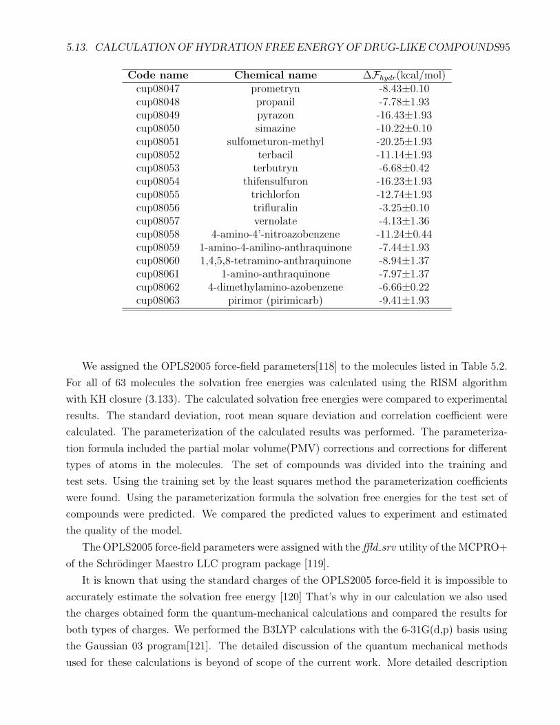
5.13. CALCULATION OF HYDRATION FREE ENERGYOF DRUG-LIKE COMPOUNDS95
Code name Chemical name ∆Fhydr(kcal/mol)cup08047 prometryn -8.43±0.10cup08048 propanil -7.78±1.93cup08049 pyrazon -16.43±1.93cup08050 simazine -10.22±0.10cup08051 sulfometuron-methyl -20.25±1.93cup08052 terbacil -11.14±1.93cup08053 terbutryn -6.68±0.42cup08054 thifensulfuron -16.23±1.93cup08055 trichlorfon -12.74±1.93cup08056 trifluralin -3.25±0.10cup08057 vernolate -4.13±1.36cup08058 4-amino-4’-nitroazobenzene -11.24±0.44cup08059 1-amino-4-anilino-anthraquinone -7.44±1.93cup08060 1,4,5,8-tetramino-anthraquinone -8.94±1.37cup08061 1-amino-anthraquinone -7.97±1.37cup08062 4-dimethylamino-azobenzene -6.66±0.22cup08063 pirimor (pirimicarb) -9.41±1.93
We assigned the OPLS2005 force-field parameters[118] to the molecules listed in Table 5.2.
For all of 63 molecules the solvation free energies was calculated using the RISM algorithm
with KH closure (3.133). The calculated solvation free energies were compared to experimental
results. The standard deviation, root mean square deviation and correlation coefficient were
calculated. The parameterization of the calculated results was performed. The parameteriza-
tion formula included the partial molar volume(PMV) corrections and corrections for different
types of atoms in the molecules. The set of compounds was divided into the training and
test sets. Using the training set by the least squares method the parameterization coefficients
were found. Using the parameterization formula the solvation free energies for the test set of
compounds were predicted. We compared the predicted values to experiment and estimated
the quality of the model.
The OPLS2005 force-field parameters were assigned with theffld srv utility of the MCPRO+
of the Schrodinger Maestro LLC program package [119].
It is known that using the standard charges of the OPLS2005 force-field it is impossible to
accurately estimate the solvation free energy [120] That’s why in our calculation we also used
the charges obtained form the quantum-mechanical calculations and compared the results for
both types of charges. We performed the B3LYP calculations with the 6-31G(d,p) basis using
the Gaussian 03 program[121]. The detailed discussion of the quantum mechanical methods
used for these calculations is beyond of scope of the current work. More detailed description

96 CHAPTER 5. RISM MULTI-GRID ALGORITHM
of B3LYP method can be found in Ref. [122]. The partial charges of the molecules were
calculated using the CHELPG (CHarges form Electrostatic Potential, Grid method), which
assumes that the partial charges were assigned in such a way that the electrical potential in
some chosen points is equal in classical and quantum mechanical approximations[123]. In the
standard procedure for calculating CHELPG charges there are no parameters for the Bromine
atom. In our quantum calculations we changed the Bromine atom in the molecule Cup08013 to
the Chlorine atom. For the numerical solution of the RISM equations (5.1) one need to know
solute intermolecular functions ωss′(k), solvent susceptibility functions χαα′(k) and pairwise
site-site potentials usα(r). The intermolecular functions can be simply calculated from the 3D
structure of the solute molecule. In the Fourier space the expressions for these functions can
be represented in a following way:
ωss′(k) =sin krss′
krss′(5.97)
where rss′ is the distance between the atoms s and s′ of the solute molecule. We perform RISM
and SFE calculations for the temperature T = 300K. We use the susceptibility functions from
Ref. [83] where these functions were calculated by using the wavelet-based algorithm for solving
RISM equations [84, 85, 56]. The site-site potential used in this work is a superposition of the
Coulomb potential uCsα(r) and Lennard-Jones potential uLJ
sα (r), namely:
usα(r) = uCsα(r) + uLJ
sα (r) (5.98)
The Coulomb potential is defined in a following way:
uCsα(r) =
qsqαr
(5.99)
where qs, qα are partial charges of the atoms s and α. We use atomic units to avoid scaling
a coefficient in Coulomb potential. The unite charge is the positron charge (e) and distance
between the atoms r is given in Bohr units (1 Bohr ≈ 0.52917 A ). Pair Lennard-Jones potential
is defined with a following relation:
uLJsα (r) = 4ǫsα
((σsα
r
)12
−(σsα
r
)6)
(5.100)
Pairwise parameters σsα, ǫsα are calculated from the atomic OPLS2005 parameters σs, σα, ǫs,
ǫα using the Lorentz-Berthelot mixing rules:
σsα =σs + σα
2ǫsα =
√ǫsǫα (5.101)
We note, that the standard OPLS2005 mixing rules differ from the Lorentz-Berthelot rules.
In OPLS2005 force-field it is assumed that σsα =√σsσα. The reason why we are using the
5.13. CALCULATION OF HYDRATION FREE ENERGYOF DRUG-LIKE COMPOUNDS97
Lorentz-Berthelot rules in our work is that for standard OPLS2005 rules the RISM equation
solver diverges for some molecules. In our work we use the modified SPC/E water model
(MSPC/E) [124]. The MSPC/E water model in contrast to the standard SPCE model [125]
has non-zero LJ potential for the Hydrogen atom. In our work we use the following Hydrogen
LJ parameters: σH = 0.8A, ǫH = 0.046 kcal/mol. The RISM and SFE calculations were
performed for the aqueous solutions at the temperature T = 300K and water density ρ = 33.7
particles/nm3. The calculations were performed with the RISM-MOL multi-grid solver[117]. In
our work the eight-level multi-grid method was used. The correlation functions were obtained
on the equispaced grid with the grid size 0.265A and 4096 discretization points. The KH-
closure was used for calculations. The calculations were performed for all the molecules listed
in Table 5.2. Two calculations for each molecule were performed: for OPLS2005 and CHELPG
partial charges correspondingly. Average computation time was 15 sec/molecule. After solving
the RISM equations the solvation free energy was calculated using four different expression:
KH, HNCB, GF, PW.
The results of the RISM SFE calculations were compared to the experimentally measured
values. We calculated the mean error, standard deviation (SD) and root mean squared devi-
ation(RMSD). The mean value and the standard deviation were calculated with the following
expressions:
M(∆G−∆Gexp) =1
N
∑
i∈S
(∆G(i) −∆G(i)
exp
)(5.102)
SD(∆G−∆Gexp) =√
1
N
∑
i∈S
(∆G(i) −∆G(i)
exp −M(∆G−∆Gexp))2 (5.103)
The RMSD can be calculated with the following formula:
RMSD(∆G, ∆Gexp)2 =
M(∆G−∆Gexp)2 + SD(∆G−∆Gexp)
2 (5.104)
In Ref. [37] it is shown that the partial molar volume (PMV) correction can essentially
increase the accuracy of the RISM SFE calculations for simple non-polar compounds. This
suggests that the parameterization of the SFE for the compounds from the SAMPL1 set can
also be useful.
In the RISM approximation the partial molar volume can be calculated as a limiting case
for the infinite dilution using the general formula for the partial molar volume[126]. This gives
the following expression for the PMV of the solute molecule:
Vex =1
ρ+
4π
Nsolute
∑
s
∞∫
0
(hsolvoo (r)− hso(r)
)r2dr. (5.105)

98 CHAPTER 5. RISM MULTI-GRID ALGORITHM
where hsolvoo is a total oxygen-oxygen correlation function of a pure water, hso(r) is a total cor-
relation function between the solute site s and water oxygen. For the parameterization it is
convenient to use dimensionless value. So we use the dimensionless value ρVex where ρ is a water
density. In Ref. [37] the systematic overestimation of the hydrogen-bond contribution to the
SFE in the RISM calculations for the molecules with highly charged groups is discussed. The
authors introduce the hydrogen-bond correction which accounts the number of hydroxyl groups
in the molecule. In our work we use the similar method. However, because the compounds in
the SAMPL1 set are much more complicated than ones in Ref. [37] we do not see the simple
way to divide these compounds into functional groups. Thus we simply introduce corrections
for each type of atoms in the molecule. The molecules in Table 5.2 contain Hydrogen, Carbon,
Oxygen, Nitrogen, Sulfur, Phosphorus, Chlorine, Fluorine and Bromine. To reduce the num-
ber of parametrization coefficients we do not distinguish Fluorine, Chlorine and Bromine and
introduce one Halogen correction (F,Cl,Br). We use the following parameterization formula:
∆Gcorr(b) = ∆GRISM + bV ρVex +∑
j
bjnj (5.106)
where summation is done over all atom types j ∈ H, C, N , O, Hal, P , S ( Hal means halo-
gen), nj is a number of atoms of type j in the molecule, b = bV , bH , bC , bN , bO, bHal, bP , bSare the parameterization coefficients. To calculate the parameterization coefficients the set of
compounds from Table 5.2 was divided into the training and test sets. The training set of com-
pounds is composed from all the compounds those codes end up with an odd digit (Cup08001,
Cup08003, . . . , Cup08063), the training set of compounds includes all the compounds those
numbers end up with a even digit (Cup08002, Cup08004, . . . , Cup08062). Coefficients b = bV ,
bH , bC , bN , bO, bHal, bP , bS were calculated with the least squares method on the training set
of compounds. In such a way the exact expression for prediction the solvation free energies was
determined. Using this formula the SFE of the compounds from the test set were calculated.
The results of the calculations were compared to the experimental values.
The results of the free energy calculations for different SFE expressions and OPLS2005 and
CHELPG charges are presented in Table 5.3. Sorting the results in ascending RMSD order we
can see that the worst results gives the KH expression, HNCB is the next one, the error of PW
and GF are approximately equal. We note that in case of PW expression the most contribution
to RMSD gives the systematic mean error shift while in GF formula the most contribution is due
to dispersion. All the expressions show not very big correlation with experiment. However for
all expression except KH the correlation coefficient is greater than 0.5. The largest correlation
with experiment is for the HNCB expression. This can be explained by the fact that the
additional repulsive potential introduced in (4.34) can be regarded as some kind of partial
molar volume correction. And this in turn means that despite the fact that HNCB results

5.13. CALCULATION OF HYDRATION FREE ENERGYOF DRUG-LIKE COMPOUNDS99
Table 5.3: Results of the RISM solvation free energy calculations. In the table the data forthe differences between the experimental and calculated data are presented: RMSD, meandeviation (M), standard deviation (SD) and correlation coefficient. Data is given in kcal/mol.Expression Charges RMSD M SD Correlation Coefficient
PW OPLS2005 11.366 9.978 5.442 0.637GF OPLS2005 11.932 -6.778 9.820 0.603
HNCB OPLS2005 14.084 -5.753 12.855 0.803KH OPLS2005 75.665 72.660 21.112 0.119PW CHELPG 12.758 -12.153 3.883 0.690GF CHELPG 8.421 4.139 7.333 0.651KH CHELPG 78.844 -75.362 23.173 0.065
HNCB CHELPG 11.985 2.870 11.636 0.794
correlate with the experimental measurements they could not be essentially improved by the
partial molar volume parameterization (this is shown below). Comparing results for CHELPG
and OPLS2005 charges we see that CHELPG charges provide better results. Although the
mean value of the error (M) and RMSD weakly depend on the partial charges. But in case of
the CHELPG charges standard deviation of the error is essentially smaller, which suggests that
the data calculated with CHELPG charges can be effectively parameterized.
The results of the calculations were parameterized using the expression (5.106) for KH,
HNCB, GF, PW solvation free energy expressions. In Table 5.4 the values of RMSD, mean
error and standard deviation of error on the test set of compounds are presented. To prove
additionally the necessity of RISM calculations we also performed “pure chemoinformatic”
parameterization without calculating solvation free energies. To do it we put to the formula
(5.106) zero instead of ∆G and perform the parameterization. We see that the best of OPLS2005
results is calculated with PW formula. The RMSD for this method is 3.1 kcal/mol, while pure
chemoinformatic parameterization for the same compounds gives an error 2.8 kcal/mol. So
OPLS2005 charges should not be used for SFE prediction.
In contrast to unsatisfactory results for OPLS2005 charges, the parameterization for CHELPG
charges allows to predict the SFE with RMSD=1.9 kcal/mol for the PW expression, which is
almost 1.5 times better than the best “pure chemoinformatics” result. Result for GF formula
(RMSD=2.5 kcal/mol) still can slightly improve the chemoinformatics result. KH and HNCB
expression show unsatisfactorily results (RMSD > 5 kcal/mol). We note that although HNCB
method without parameterization shows better results than KH, after the parameterization KH
becomes more effective. Coefficients b = bV , bH , bC , bN , bO, bHal, bP , bS for the CHELPG/PW
method are given in Table 5.5. Analyzing the coefficients we see that the most contribution to
the correction gives the Partial Molar Volume correction while other corrections are in average
4-5 times smaller.

100 CHAPTER 5. RISM MULTI-GRID ALGORITHM
Table 5.4: Results of parameterization for KH, HNCB, GF, PW expressions. In the tablethe following data for differences between the calculated and experimental values are given:RMSD, standard deviation (SD), mean error (M), correlation coefficient. Units in all casesare kcal/mol. The line with the expression “none” correspond to the pure chemoinformaticsparameterization.Expression Charges RMSD M SD Correlation coefficient
PW OPLS2005 3.075 -0.173 3.070 0.803GF OPLS2005 3.690 -0.378 3.671 0.791KH OPLS2005 5.541 -1.132 5.424 0.775
HNCB OPLS2005 6.902 -1.706 6.688 0.767none OPLS2005 2.837 0.350 2.815 0.651PW CHELPG 1.913 0.382 1.875 0.927GF CHELPG 2.542 0.375 2.514 0.912KH CHELPG 5.024 -0.318 5.013 0.825
HNCB CHELPG 6.197 -0.680 6.159 0.819none CHELPG 2.845 0.342 2.824 0.638
Table 5.5: Values of the parameterization coefficients for CHELPG/PW method. Units -kcal/molCoefficient Value
bV -7.773bH 0.797bC 1.578bN 1.466bO 1.863bHal 2.851bP 3.152bS 4.982
5.14. CONCLUSIONS 101
5.14 Conclusions
We described a new multi-grid-based algorithm for solving RISM equations. We adopted a
general non-linear multi-grid scheme for solving the RISM equations. We also proposed an
extension of the algorithm for the grids with different cutoff distances. Additionally we investi-
gated the efficiency of the coarse-grid solver and proposed an adaptive algorithm for calculating
the optimal number of iteration steps on the coarsest grid. We performed numerical investi-
gations to optimize the algorithm parameters to give the required numerical accuracy of the
Hydration Free Energy calculations by RISM. The investigated parameters were: fine-grid cut-
off distance, fine-grid discretization step, coarsest grid cutoff distance and coarsest grid size.
By numerical tests on polar and non-polar simple and multi-atom molecules it was shown that
RISM calculations with a fine grid 4096, 0.05 Bohr are able to give a numerical accuracy of
the Hydration Free Energy value of 0.001 kcal/mol, which is satisfactory for most of the chemi-
cal applications. It was shown that the multi-grid calculations with coarsest grid 32, 0.8 Bohrare optimal.
The proposed multi-grid methods were compared to the one-grid Picard iteration scheme,
which is the reference algorithm, and to the nested Picard iteration algorithm, which is the
most straightforward implementation of the multi-scale scheme. It was shown that for high
accuracies the proposed methods are about 30 times faster than the single-grid Picard itera-
tion, and almost 7 times faster than the nested Picard iteration. The solvation free energy
calculations for the SAMPL1 set of drug-like compounds from the paper [93] were performed
with the RISM multi-grid algorithm. The force-field for the calculation included LJ parameters
from the OPLS2005 force-field. Two types of the partial charges (OPLS2005 and CHELPG)
were used. Solvation free energy calculations were performed using the KH, HNCB, GF, PW
expressions. The calculated results for all expressions except KH have the correlation with
the experimental data. However, the results without parameterization cannot be considered
as satisfactorily (RMSD > 5 kcal/mol). The parameterization of the calculation results was
performed. The parameterization formula included corrections for partial molar volume and
number of atoms of each type in the mole The parameterization results showed that calcula-
tions with OPLS2005 charges do not give satisfactorily results (RMSD for the best method is
3.1 kcal/mol). In contrast, parameterization for the CHELPG charges showed that the RMSD
for the best method (CHELPG/PW) is 1.9 kcal/mol which is almost 1.5 fold better than the
verification “pure chemoinformatic” parameterization. Thus we conclude that although RISM
solvation free energy calculations do not immediately give the perfect results, after proper pa-
rameterization one can get the expression which is able to predict solvation free energies with
reasonable accuracy ( 1.9 kcal/mol). We also note that results depend on the correct choice of
partial charges calculation and also on RISM SFE expression.

Chapter 6
3DRISM Multi-grid Algorithm for Fast
Solvation Free Energy Calculations
In this chapter the multi-grid algorithm for solving 3DRISM equations is described and tested
on a set of organic compounds. The chapter is based on Ref. [127].
6.1 Iterative solution of the 3DRISM equations
In our work we use the Kovalenko-Hirata formulation of the 3D RISM theory [115, 128] in
order to describe infinitely diluted solutions of small organic solute molecules. Solvent (wa-
ter) molecules are described by the RISM approximation, while a solute molecule is a three-
dimensional object. Structure of the solvent is described by the total and direct correlation
functions hα(r), cα(r) where α indicates a solvent site. The 3DRISM equations are written in
the following way:
hα(r) =
Nsolvent∑
ξ=1
∫
R3
cξ(r′)χξα(r− r′)dr′ (6.1)
where Nsolvent is the number of solvent sites, χξα(r) is the solvent susceptibility function for
sites ξ and α. Solvent susceptibility functions χξα(r) are defined as following:
χξα(r) = ωξα(r) + ρhsolvξα (r), (6.2)
where r = |r|, ωξα(r) = δξα+(1− δξα)δ(r− rξα)/(4πr2ξα), rξα is the distance between the sites ξ
and α of a solvent molecule, hsolvξα (r) is the total site-site correlation function of the solvent sites
ξ and α, δξα is the Kronecker delta and δ(r) is the Dirac delta function. We used the functions
hsolvξα (r) calculated in [38].
(6.1) is completed by closure relations:
hα(r) = e−βUα((r))+hα(r)−cα(r)+Bα(r) − 1, (6.3)
102

6.1. ITERATIVE SOLUTION OF THE 3DRISM EQUATIONS 103
where β = 1/kBT , kB is the Boltzmann constant, T is the temperature, Uα(r) is the interaction
potential corresponding to a solute site α, Bα(r) is the bridge functional.
To use iterative solvers we rewrite (6.1) in the following form [129]:
γα(r) =
Nsolvent∑
ξ=1
∫
R3
C[γξ(r′ − r)] · χξα(r′)dr′ + θα(r)− C[γα(r)] (6.4)
where γα(r) = hα(r)− cSα(r), cSα(r) = cα(r) + βUL
α (r), Uα(r) = USα (r) + UL
α (r), USα (r) is a short
range potential, ULα (r) is a long range potential, θα(r) = −β
∑
ξ
∫
R3 ULξ (r− r′)χξα(r
′)dr′, C[·] isa closure (bridge) functional.
We use interaction potentials which are superpositions of the site-site interaction potentials:
USα (r) =
Nsolute∑
s=1
uSsα(|r− rs|); (6.5)
ULα (r) =
Nsolvent∑
s=1
uLsα(|r− rs|); (6.6)
where rs is the position of a solute site s with respect to the center of a molecule, Nsolute is the
number of solute sites. In our work the site-site potentials contain Lennard-Jones and Coulomb
part. Pair Lennard-Jones parameters are obtained from the atomic LJ parameters by using the
Lorentz-Berthelot mixing rules:
σsα =1
2(σs + σα) ǫsα =
√ǫsǫα (6.7)
To avoid divergence of the algorithm due to the long range behavior of the interaction potentials
we separate the short range and the long range of the potentials that we then treat separately by
using the Ng procedure [116]. We use the atomic units for distance and energy Bohr=0.52918 ·10−10m and Hartree=4.35974394 · 1018 J. This allows us to avoid scaling coefficients in the
representation of the Coulomb potential. Thus expressions for the short-range and long-range
potentials are written as following:
uSsα(r) = uLJ(short)
sα (r) + uCsα(r)(1− erf(τr)) (6.8)
uLsα(r) = uLJ(long)
sα (r) + uCsα(r)erf(τr) (6.9)
where uCsα(r) is the Coulomb component of the site-site potential, erf(r) =
∫ r
−∞ e−t2dt, τ=0.5
Bohr−1, uLJ(short)sα (r), u
LJ(long)sα (r) are short-range and long-range components of the Lennard-
Jones potential respectively. The latter are defined by the following relations:
uLJ(short)sα (r) =
uLJsα (r)− uLJ
sα (Rcut) when r < Rcut
0 otherwise(6.10)

104 CHAPTER 6. 3DRISM MULTI-GRID ALGORITHM
Figure 6.1: Spacing is the minimal distance between the grid points, buffer is the minimaldistance from the solute atoms to the boundaries of the grid
uLJ(long)sα (r) = uLJ
sα (r)− uLJ(short)sα (r) (6.11)
where uLJsα (r) is a Lennard-Jones component of a site-site potential, Rcut=8A .
In the article we use the Kovalenko-Hirata (KH) closure, which is defined as following [130]:
C[γα(r)] =
e−βUSα (r)+γα(r) − γα(r)− 1 when − βUS
α (r) + γα(r) > 0−βUS
α (r) otherwise(6.12)
In the numerical representation of (6.4) the functions γα(r), χξα(r), θα(r) are defined by
their values in the grid points of an uniform Cartesian grid. A grid is defined by two param-
eters: spacing and buffer. Spacing is the smallest distance between the grid points and buffer
is the minimal distance from the solute atoms to the boundaries of the grid (see Figure 6.1
for explanations). At first glance, such parameterization may seem to be inconvenient from
a theoretical point of view because the same buffer and spacing parameters may give differ-
ent grids for different solutes. However, our work is mostly oriented towards future practical
applications of the method and in practical applications we are interested in the accuracy of
calculations for different cutoff distances of the correlation functions; and these cutoff distances
for a Cartesian grid are defined by the buffer parameter. Using the same buffer parameter
we can adjust the size and the shape of the grid preserving a constant cutoff of the solvent
correlation functions for different solutes. That provides us a straightforward way to control
the accuracy of calculations.

6.2. DIIS AND MDIIS ITERATION 105
We denote the forward and the inverse Fourier transforms on the grid G as TG [·], T −1G [·]
correspondingly. Then a discrete analogue of (6.4) reads as:
ΓG = T −1G
[
X · TG[C[ΓG]]
]
+ΘG − C[ΓG] (6.13)
where ΓG =(γG1 , . . . ,γ
GNsolvent
)T, ΘG =
(θG1 , . . . ,θ
GNsolvent
)T, XG = [χG
ξα]Nsolvent×Nsolvent, χG
ξα =
FG[χξα], upper index G means that functions are given by their values in the grid points of the
grid G.Equation (6.13) can be written in a more compact way:
ΓG = F [ΓG] (6.14)
where F [ΓG] = T −1G
[
X · TG[C[ΓG]]
]
+ΘG − C[ΓG].
The Picard iteration method is defined by the following recurrent formula:
ΓGn+1 = (1− λ)ΓG
n + λF [ΓGn] (6.15)
where ΓGn is the n-th step approximation, λ is the coupling parameter.
6.2 DIIS and MDIIS iteration
Direct inverse in the iterative subspace (DIIS) method is an iteration method initially in-
troduced to improve convergence of Schrodinger equation solvers [131]. Later modified DIIS
(MDIIS) method was applied to the 3DRISM equations [77]. In the DIIS method on the n-
th iteration step one finds an approximate solution ΓG∗ which is a linear combination of the
approximations on the k previous iteration steps:
ΓG∗ =
k∑
i=1
CiΓGn−k+i (6.16)
Below we describe the DIIS and MDIIS algorithms which solve the 3DRISM equations in
the form (6.14). We also plan to use the MDIIS algorithm in our multi-grid scheme. This will
require to consider a generalized task in the following form:
ΓG = F [ΓG] +DG (6.17)
where DG =(dG1 , . . . ,d
GNsolvent
)Tis an arbitrary vector of corrections. The vector of corrections
will be calculated during the multi-grid algorithm when we move from one grid to another
one. This procedure is described in the next section. In the current section we describe one-
grid solvers where vector DG is given. Below we describe the DIIS and MDIIS algorithms for
106 CHAPTER 6. 3DRISM MULTI-GRID ALGORITHM
a general case of an arbitrary vector D having in mind that the 3DRISM equations (6.14)
correspond to the case DG ≡ 0.
In the DIIS method the coefficients Ci in (6.16) are chosen to minimize the norm of the
residue ∆G∗ = ΓG
∗ − F [ΓG∗ ]−DG. If one assumes linearity of the operator F (which for smooth
operators is locally true) then the task reduces to the following system of linear equations[131]:
a11 . . . a1k −1...
. . .... −1
ak1 . . . akk −11 . . . 1 0
C1...Ck
λ
=
0...01
(6.18)
where aij =∫
R3 ∆i(r)∆j(r)dr, ∆i(r) = ΓGn−k+i − F [ΓG
n−k+i] − DG. In the DIIS method ΓG∗ is
used as a solution approximation on the (n+1)-st iteration step. However, such a procedure
can lead to a linearly dependent system of equations. The MDIIS iteration method avoids this
problem by adding a weighted residue to the (n+1)-st step approximation [77]:
Γ′G = ΓG∗ + η
(F [ΓG
∗ ] +DG − ΓG∗)
(6.19)
where η is a weight for the residue. In combination with the standard damping technique the
solution approximation on the (n+1)-st step ΓGn+1 in the MDIIS method can be found by using
the following formula:
ΓGn+1 = (1− λ)ΓG
n + λΓG∗ + λη
(F [ΓG
∗ ] +DG − ΓG∗)
(6.20)
In our work we use λ = 0.5, η = 0.3. These values are sub-optimal and allow to ensure stability
of the algorithm and in the same time retain reasonable performance. Detailed description of
the dependence of the computation time on λ and η parameters is given below.
To make notations shorter we introduce the MDIIS operator Ξ[·, ·]:
Ξ[ΓGn,D
G ] = (1− λ)ΓGn + λΓG
∗ + λη(F [ΓG
∗ ] +DG − ΓG∗)
(6.21)
6.3 Multi-grid
We use the multi-grid technique in order to decrease the computation time spent on solving the
3DRISM equations. General description of the multi-grid theory can be found in the book [87].
Here we give only short description of the multi-grid method applied to the 3DRISM equations.
More information on the theoretical background of the method can be found in the previous
chapter.
In the multi-grid method the numerical task is discretized on several grids with the same
buffer but different spacings. Grids with smaller numbers of points and larger spacings are

6.3. MULTI-GRID 107
called coarse grids, grids with larger number of the points and smaller spacings are called fine
grids. In our work we consider grids where number of points differ by the factor of 2n, where
n = 0, 1, 2, ....
We introduce operators p[·], r[·], which convert a coarse grid to a finer one and vice versa.
We introduce an operator R[·] which map a fine-grid function to a coarse grid.
R[ΓG ] = Γr[G] (6.22)
Also we introduce an operator P [·] which interpolates a coarse-grid function to a fine grid:
P [Γr[G]] = ΓG1 (6.23)
We use the linear interpolation operator.
To make notations simpler we introduce an operator Λ[·; ·]:
Λ[ΓG ;DG ] = (1− λ)ΓG + λ
(FG[Γ
G] +DG) . (6.24)
A multi-grid iterative algorithm which solves the task (6.17) can be written in the following
form:
ΓGn+1 = Ml
G[ΓG
n;DG] , (6.25)
where ΓGn is the n-th step approximation, Ml
G[·; ·] is a multi-grid operator which performs one
multi-grid iteration step of the depth l on the grid G. To calculate the multi-grid operator
of the depth l = 0 one performs m0 one-grid iteration steps on the grid G. The multi-grid
technique can be applied to both: the Picard and the MDIIS iteration methods. We define a
generalized operator Φ[·; ·] in the following way:
Φ[ΓGn;D
G ] =
Λ[ΓG
n;DG ] for MG-Picard method
Ξ[ΓGn;D
G ] for MG-MDIIS method(6.26)
Then the multi-grid operator of the depth l = 0 is defined as:
M0G[ΓG;DG] = Φm0
[ΓG;DG] (6.27)
For l > 0, given the n-th step approximation ΓGn and the correction vectorDG, the multi-grid
operator MlG[·; ·] is calculated by the following algorithm:
Input parameters: ΓGn, D
G , l
Result: ΓGn+1 = Ml
G[ΓGn;D
G ]
1. Perform ν1 Picard iteration steps on the fine grid (in our work ν1 = 5):
Γ′G = Λν1[ΓG
n;DG]

108 CHAPTER 6. 3DRISM MULTI-GRID ALGORITHM
2. Move to the coarse grid r[G]:Γ
r[G](0) = R[Γ′G ];
3. Calculate the coarse-grid correction:
Er[G] = R[F [Γ′G ]
]− F [Γ
r[G](0) ]
4. Perform recursively µ multi-grid iteration steps of depth l − 1 on the coarse-grid (in our
work µ=1):
Γr[G](µ) =
(
Ml−1r[G]
)µ [
Γr[G](0) ;R[DG ] + Er[G]
]
5. Correct the fine-grid solution using the coarse-grid results:
Γ′′G = Γ′G + P[
Γr[G](µ) − Γ
r[G](0)
]
6. Perform ν2 Picard iteration steps on the fine grid (in our work ν2 = 0):
ΓGn+1 = Λν2
[Γ′′G;DG]
The number of the iteration steps m0 in the multi-grid operator of the depth l = 0 depends
on the number of the multi-grid iteration step n: m0 = m0(n). We define m0(n) in such a way
that after m0(n) iteration steps, a residue decays by the factor Kn:
Kn||Φm0(n)[ΓGn;D
G ]− Φm0(n)+1[ΓGn;D
G ]|| < ||ΓGn − Φ[ΓG
n;DG ]|| (6.28)
We call the value Kn the decay factor.
Constant decay factor may lead to a non-smooth decay of residue from one multi-grid
iteration step to another which in turn leads to increasing of the number of the idle coarse-grid
iteration steps (see Figure 6.2, solid line). To achieve a smoother decay of the error, in our
work we change Kn by the following recursive formula:
Kn+1 =
max( 1
αKn, Kmin) if ||ΓG
n,m0− Φ[ΓG
n,m0;DG ]|| < ||ΓG
n+1 − Φ[ΓGn+1;D
G ]||min(βKn, Kmax) otherwise
(6.29)
where ΓGn,m0
= (ΦG)m0(n)[ΓG
n;DG ], α = 2, β = 1.2. For the MG-Picard method we use K0 = 10,
Kmin = 5, Kmax = 100, for the MG-MDIIS method we use K0 = 100, Kmin = 10, Kmax = 100.
This allows us to smooth the decay of error and to reduce the total number of the iteration
steps (see Figure 6.2, dashed line).
Usually iterative algorithms stop when the norm of the residue is less than some threshold.
However, this method has its own disadvantages. The first one is that a small residue between
two iteration steps does not necessarily imply a small distance from the current approximation
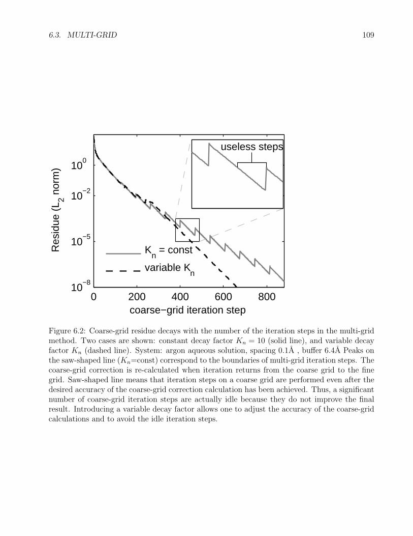
6.3. MULTI-GRID 109
0 200 400 600 80010
−8
10−5
10−2
100
coarse−grid iteration step
Res
idue
(L 2 n
orm
)
Kn = const
variable Kn
useless steps
Figure 6.2: Coarse-grid residue decays with the number of the iteration steps in the multi-gridmethod. Two cases are shown: constant decay factor Kn = 10 (solid line), and variable decayfactor Kn (dashed line). System: argon aqueous solution, spacing 0.1A , buffer 6.4A Peaks onthe saw-shaped line (Kn=const) correspond to the boundaries of multi-grid iteration steps. Thecoarse-grid correction is re-calculated when iteration returns from the coarse grid to the finegrid. Saw-shaped line means that iteration steps on a coarse grid are performed even after thedesired accuracy of the coarse-grid correction calculation has been achieved. Thus, a significantnumber of coarse-grid iteration steps are actually idle because they do not improve the finalresult. Introducing a variable decay factor allows one to adjust the accuracy of the coarse-gridcalculations and to avoid the idle iteration steps.
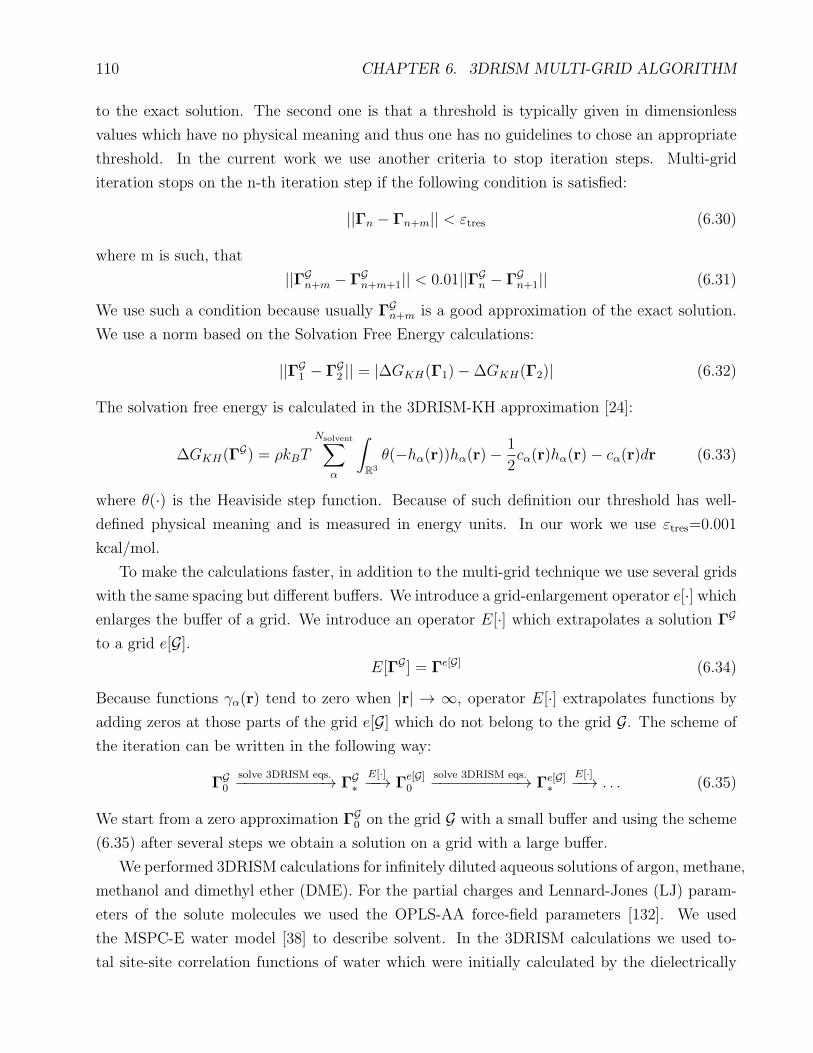
110 CHAPTER 6. 3DRISM MULTI-GRID ALGORITHM
to the exact solution. The second one is that a threshold is typically given in dimensionless
values which have no physical meaning and thus one has no guidelines to chose an appropriate
threshold. In the current work we use another criteria to stop iteration steps. Multi-grid
iteration stops on the n-th iteration step if the following condition is satisfied:
||Γn − Γn+m|| < εtres (6.30)
where m is such, that
||ΓGn+m − ΓG
n+m+1|| < 0.01||ΓGn − ΓG
n+1|| (6.31)
We use such a condition because usually ΓGn+m is a good approximation of the exact solution.
We use a norm based on the Solvation Free Energy calculations:
||ΓG1 − ΓG
2 || = |∆GKH(Γ1)−∆GKH(Γ2)| (6.32)
The solvation free energy is calculated in the 3DRISM-KH approximation [24]:
∆GKH(ΓG) = ρkBT
Nsolvent∑
α
∫
R3
θ(−hα(r))hα(r)−1
2cα(r)hα(r)− cα(r)dr (6.33)
where θ(·) is the Heaviside step function. Because of such definition our threshold has well-
defined physical meaning and is measured in energy units. In our work we use εtres=0.001
kcal/mol.
To make the calculations faster, in addition to the multi-grid technique we use several grids
with the same spacing but different buffers. We introduce a grid-enlargement operator e[·] whichenlarges the buffer of a grid. We introduce an operator E[·] which extrapolates a solution ΓG
to a grid e[G].E[ΓG] = Γe[G] (6.34)
Because functions γα(r) tend to zero when |r| → ∞, operator E[·] extrapolates functions by
adding zeros at those parts of the grid e[G] which do not belong to the grid G. The scheme of
the iteration can be written in the following way:
ΓG0
solve 3DRISM eqs.−−−−−−−−−−→ ΓG∗
E[·]−−→ Γe[G]0
solve 3DRISM eqs.−−−−−−−−−−→ Γe[G]∗
E[·]−−→ . . . (6.35)
We start from a zero approximation ΓG0 on the grid G with a small buffer and using the scheme
(6.35) after several steps we obtain a solution on a grid with a large buffer.
We performed 3DRISM calculations for infinitely diluted aqueous solutions of argon, methane,
methanol and dimethyl ether (DME). For the partial charges and Lennard-Jones (LJ) param-
eters of the solute molecules we used the OPLS-AA force-field parameters [132]. We used
the MSPC-E water model [38] to describe solvent. In the 3DRISM calculations we used to-
tal site-site correlation functions of water which were initially calculated by the dielectrically

6.4. FINDING THE OPTIMAL GRID PARAMETERS 111
consistent RISM technique [38]. Pairwise σ Lennard-Jones parameters were calculated as an
arithmetic mean of atomic parameters, pairwise ǫ Lennard-Jones parameters were calculated
as a geometric mean of atomic parameters:
σ12 =σ1 + σ2
2; ǫ12 =
√ǫ1 · ǫ2 (6.36)
Calculations were performed on the Intel(R) Xeon(R) CPU X5650 with the clocking 2.67GHz.
For calculation of the direct and inverse fast Fourier transforms the FFTW3 library was
used[133].
6.4 Finding the optimal grid parameters
We performed 3DRISM calculations for infinitely diluted aqueous solutions of four compounds:
argon, methane, methanol and DME. To determine the optimal grid parameters we performed
solvation free energy (SFE) calculations on grids with different spacing parameters and different
buffers. In Figure 6.3 the dependence of calculation errors on the spacing parameter is shown.
For the calculations we used several different grids with the fixed buffer of 8A and different
spacings which vary from 0.1A to 2A . Errors were calculated as absolute values of the differ-
ences between SFEs calculated on a current grid and SFEs calculated on the very fine grid with
the spacing of 0.05A and the buffer of 8A . The results show that the the grid with the spacing
of 0.2A provides an error that is less than 0.1 kcal/mol for all solutes which is acceptable for
the most of chemical applications. Thus in our work we use the grid with spacing of 0.2A .
In Figure 6.4 we show the dependency of calculation errors on the grid buffer. The calcu-
lations were performed on grids with fixed spacing of 0.2A and different buffers varying from
8A to 20A . Errors were calculated as differences between the SFEs calculated on the current
grid and the SFEs calculated on the very fine grid with spacing of 0.2A and buffer of 30A .
The figure shows that the grid with the buffer of 15A is enough to provide the accuracy of SFE
calculations 6 0.1kcal/mol.
6.5 Dependencies of the computational time on the η
and λ parameters
In the Figures 6.5-6.6 the dependencies of the computational time on the λ parameter for
MG-Picard and MG-MDIIS methods are shown. We can see that generally for both methods
the computational time decrease with increasing of λ parameter. However, with the large λ
(λ > 0.9) there MG-MDIIS method diverges for some of the systems. As well, for the small
λ (λ < 0.3) the method is also non-stable (this is because when the λ is small the vectors
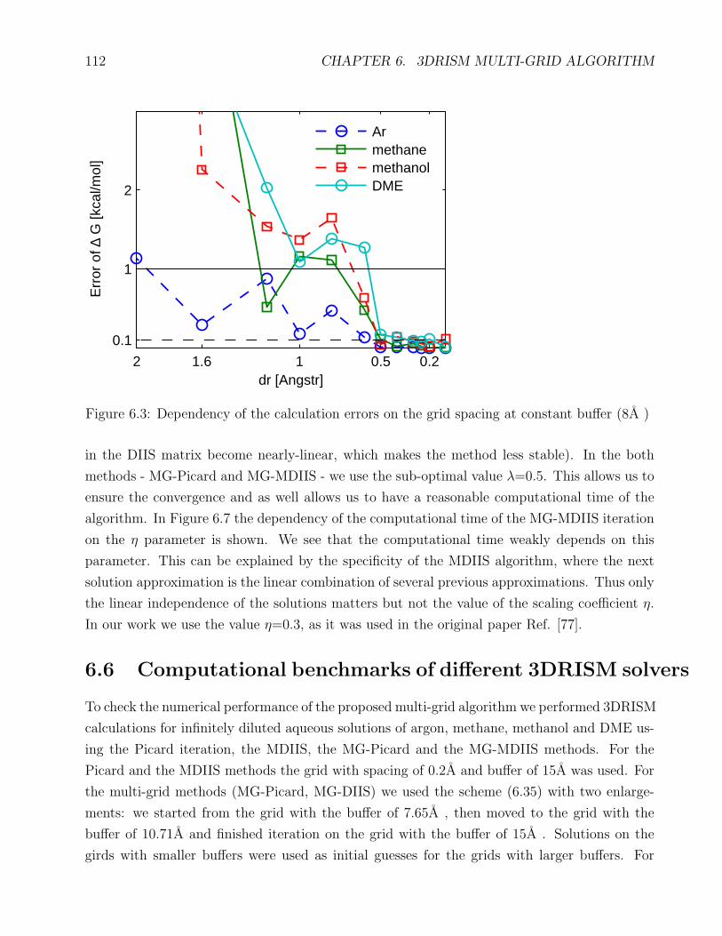
112 CHAPTER 6. 3DRISM MULTI-GRID ALGORITHM
0.20.511.62
0.1
1
2
dr [Angstr]
Err
or o
f ∆ G
[kca
l/mol
]
ArmethanemethanolDME
Figure 6.3: Dependency of the calculation errors on the grid spacing at constant buffer (8A )
in the DIIS matrix become nearly-linear, which makes the method less stable). In the both
methods - MG-Picard and MG-MDIIS - we use the sub-optimal value λ=0.5. This allows us to
ensure the convergence and as well allows us to have a reasonable computational time of the
algorithm. In Figure 6.7 the dependency of the computational time of the MG-MDIIS iteration
on the η parameter is shown. We see that the computational time weakly depends on this
parameter. This can be explained by the specificity of the MDIIS algorithm, where the next
solution approximation is the linear combination of several previous approximations. Thus only
the linear independence of the solutions matters but not the value of the scaling coefficient η.
In our work we use the value η=0.3, as it was used in the original paper Ref. [77].
6.6 Computational benchmarks of different 3DRISM solvers
To check the numerical performance of the proposed multi-grid algorithm we performed 3DRISM
calculations for infinitely diluted aqueous solutions of argon, methane, methanol and DME us-
ing the Picard iteration, the MDIIS, the MG-Picard and the MG-MDIIS methods. For the
Picard and the MDIIS methods the grid with spacing of 0.2A and buffer of 15A was used. For
the multi-grid methods (MG-Picard, MG-DIIS) we used the scheme (6.35) with two enlarge-
ments: we started from the grid with the buffer of 7.65A , then moved to the grid with the
buffer of 10.71A and finished iteration on the grid with the buffer of 15A . Solutions on the
girds with smaller buffers were used as initial guesses for the grids with larger buffers. For
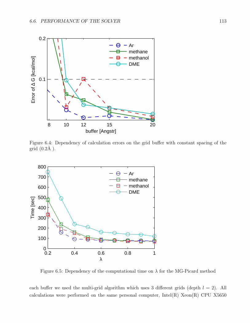
6.6. PERFORMANCE OF THE SOLVER 113
8 10 12 15 20
0.1
0.2
buffer [Angstr]
Err
or o
f ∆ G
[kca
l/mol
]
ArmethanemethanolDME
Figure 6.4: Dependency of calculation errors on the grid buffer with constant spacing of thegrid (0.2A ).
0.2 0.4 0.6 0.8 10
100
200
300
400
500
600
700
800
λ
Tim
e [s
ec]
ArmethanemethanolDME
Figure 6.5: Dependency of the computational time on λ for the MG-Picard method
each buffer we used the multi-grid algorithm which uses 3 different grids (depth l = 2). All
calculations were performed on the same personal computer, Intel(R) Xeon(R) CPU X5650

114 CHAPTER 6. 3DRISM MULTI-GRID ALGORITHM
0.2 0.4 0.6 0.8 10
100
200
300
400
500
600
λ
Tim
e [s
ec]
ArmethanemethanolDME
Figure 6.6: Dependency of the computational time on λ for the MG-MDIIS method
0.2 0.4 0.6 0.8 10
50
100
150
200
η
Tim
e [s
ec]
ArmethanemethanolDME
Figure 6.7: Dependency of the computational time on η for the MG-MDIIS method
with clocking 2.67GHz.
Computational expenses on solving 3DRISM equations for each of the investigated four
methods are presented in Table 6.1. These results show that the Picard iteration is the least
efficient method, while the most efficient is the MG-MDIIS method. We note that the multi-grid
methods in all investigated cases are more efficient than the one-grid methods.

6.6. PERFORMANCE OF THE SOLVER 115
Compound Picard iteration MDIIS MG-Picard MG-DIIS
argon 1148 sec 167 sec 46 sec 50 secmethane 1484 sec 154 sec 149 sec 82 secmethanol 1857 sec 416 sec 165 sec 83 sec
dimethyl ether 4462 sec 509 sec 241 sec 133 sec
Table 6.1: Computation expenses of 3DRISM calculations with the Picard iteration, MDIIS,MG-Picard and MG-MDIIS methods.
Ar methane methanol DME
5
10
20
spee
dup
[Tim
es]
MDIIS MG Picard MG MDIIS
Figure 6.8: Speed up of the calculations by using the MDIIS, the MG-Picard and the MG-MDIIS methods as compared to the Picard iteration method.
Figure 6.8 compares computational performance of the MDIIS, the MG-Picard and the
MG-MDIIS with the Picard iteration method. The figure shows that for all four compounds
multi-grid methods give more than 10 times speedup while for three of these four compounds
the MG-MDIIS method is more than 20 times faster than the Picard iteration method. Average
speedup factors with respect to the plain Picard method for the MDIIS, the MG-Picard and
the MG-MDIIS methods are correspondingly 7.4, 16.2 and 24.2. The most effective is the
MG-MDIIS method that is in average about 3.5 faster than the MDIIS method. Difference
between the multi-grid methods is not very large: the MG-MDIIS method is in average only
1.5 times faster than the MG-Picard method. The results show that the multi-grid scheme
can be effectively used in combination with different types of coarse-grid iteration methods for
solving the 3DRISM equations for aqueous solutions of small non-charged molecules.

116 CHAPTER 6. 3DRISM MULTI-GRID ALGORITHM
6.7 Computational benchmarks on a large set of organic
molecules
The main goal of this part of our study was to investigate the overall efficiency of the new
method in a view of large-scale practical applications like, e.g. physical-chemical profiling
of large sets of organic compounds. We performed an additional benchmark and tested the
efficiency of the new algorithm on a set of organic molecules as well as the accuracy of the
SFE prediction. We estimate average computational expenses for the 3DRISM calculations
also check whether numerical accuracy of the calculations is enough for accurate estimation of
SFE.
We have chosen a set of 99 organic molecules. This set of molecules is a part of the set
used in [74]. The list of the molecules in the set is given in the Table 6.2 and Table 6.3.The
experimental free energy values were taken from the Ref. [74]. The set includes alkanes,
ketones, alkyl-benzenes, alcohols, alkyl-phenols, ethers and other (polyfunctional) molecules.
Quantity of atoms in molecules of the set varies from 5 to 31. Average number of atoms in
a molecule is 16. The Antechamber tool [134] from the Amber Tools 1.4 Package [135] was
used for molecular structure optimization and assigning Force-Field parameters. Structures of
the molecules were optimized by using the AM1 method [136]. Atomic partial charges were
calculated by using the bond charge correction(BCC) method [137, 138]. LJ parameters from
the General Amber Force Field (GAFF) [139] were assigned to the solutes. The benchmark
calculations for simple molecules reported above show that the most effective is a combination of
the multi-grid and MDIIS(MG-MDIIS) methods. Therefore, we use the MG-MDIIS algorithm
in our benchmarking of the overall efficiency of the method.
Figure 6.9 shows dependency of the computational time spent on MG-MDIIS 3D-RISM
calculations on the number of atoms in a molecule. The plot shows that the computational
time can essentially vary for different molecules even if the molecules have the same number
of atoms. However, this somehow counterintuitive result has a straightforward explanation.
Indeed, convergence of the algorithm depends not only on the number of atoms but also on
the chemical composition of a molecule and its structure, particularly on the distribution of
atomic partial charges and the molecule surface accessible area. This is illustrated by the
results shown in Figure 6.3 and Figure 6.4 that show different error dependencies for polar and
non-polar molecules. Also, even if two different molecules have the same number of atoms,
they may still have rather different shapes. This can result in different grid sizes for them.
More compact molecules need smaller grids than the less compact molecules, even if they have
the same buffer and the same number of atoms. Therefore, combination of these two factors
causes this significant deviation of computational time for molecules of the same number of
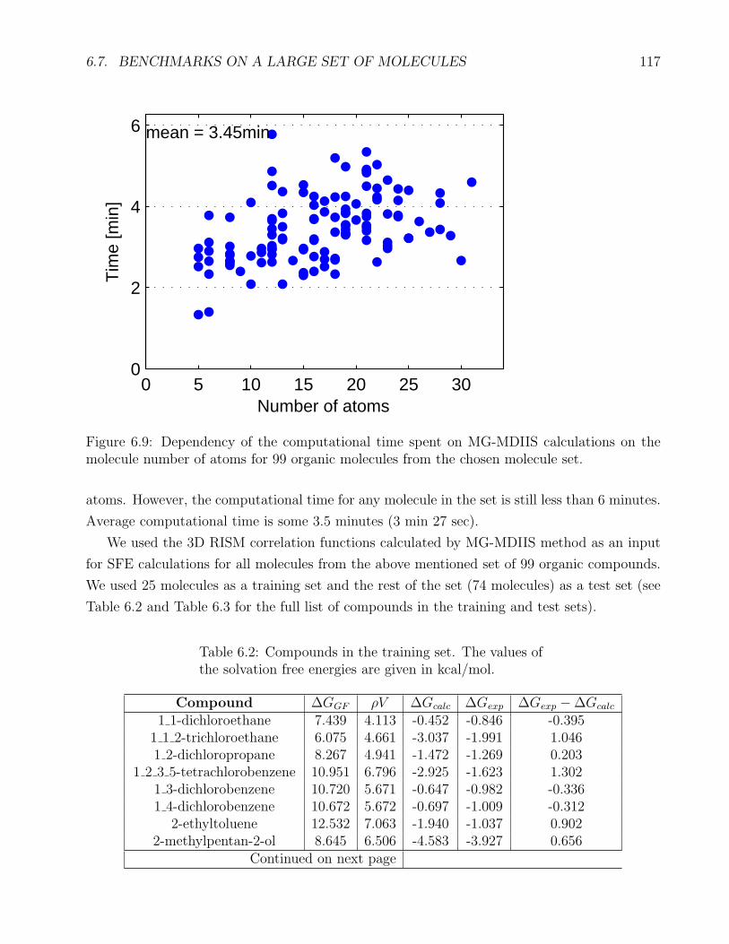
6.7. BENCHMARKS ON A LARGE SET OF MOLECULES 117
0 5 10 15 20 25 300
2
4
6
Number of atoms
Tim
e [m
in]
mean = 3.45min
Figure 6.9: Dependency of the computational time spent on MG-MDIIS calculations on themolecule number of atoms for 99 organic molecules from the chosen molecule set.
atoms. However, the computational time for any molecule in the set is still less than 6 minutes.
Average computational time is some 3.5 minutes (3 min 27 sec).
We used the 3D RISM correlation functions calculated by MG-MDIIS method as an input
for SFE calculations for all molecules from the above mentioned set of 99 organic compounds.
We used 25 molecules as a training set and the rest of the set (74 molecules) as a test set (see
Table 6.2 and Table 6.3 for the full list of compounds in the training and test sets).
Table 6.2: Compounds in the training set. The values ofthe solvation free energies are given in kcal/mol.
Compound ∆GGF ρV ∆Gcalc ∆Gexp ∆Gexp −∆Gcalc
1 1-dichloroethane 7.439 4.113 -0.452 -0.846 -0.3951 1 2-trichloroethane 6.075 4.661 -3.037 -1.991 1.0461 2-dichloropropane 8.267 4.941 -1.472 -1.269 0.203
1 2 3 5-tetrachlorobenzene 10.951 6.796 -2.925 -1.623 1.3021 3-dichlorobenzene 10.720 5.671 -0.647 -0.982 -0.3361 4-dichlorobenzene 10.672 5.672 -0.697 -1.009 -0.312
2-ethyltoluene 12.532 7.063 -1.940 -1.037 0.9022-methylpentan-2-ol 8.645 6.506 -4.583 -3.927 0.656
Continued on next page
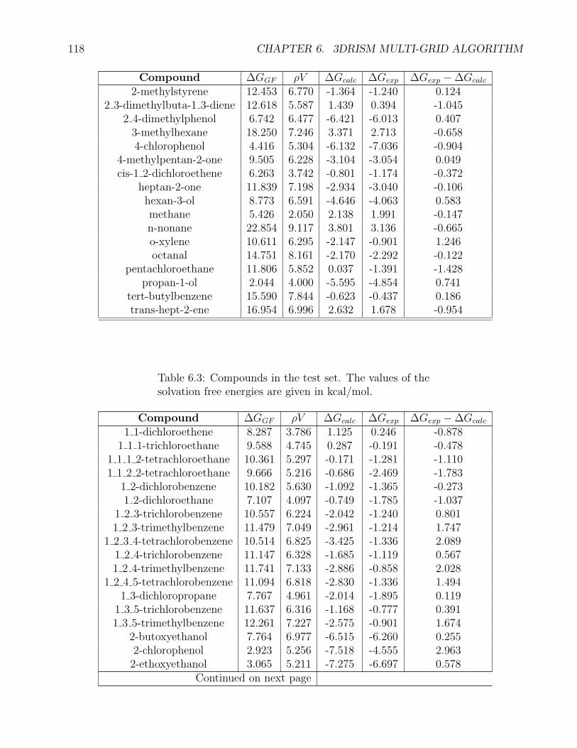
118 CHAPTER 6. 3DRISM MULTI-GRID ALGORITHM
Compound ∆GGF ρV ∆Gcalc ∆Gexp ∆Gexp −∆Gcalc
2-methylstyrene 12.453 6.770 -1.364 -1.240 0.1242 3-dimethylbuta-1 3-diene 12.618 5.587 1.439 0.394 -1.045
2 4-dimethylphenol 6.742 6.477 -6.421 -6.013 0.4073-methylhexane 18.250 7.246 3.371 2.713 -0.6584-chlorophenol 4.416 5.304 -6.132 -7.036 -0.904
4-methylpentan-2-one 9.505 6.228 -3.104 -3.054 0.049cis-1 2-dichloroethene 6.263 3.742 -0.801 -1.174 -0.372
heptan-2-one 11.839 7.198 -2.934 -3.040 -0.106hexan-3-ol 8.773 6.591 -4.646 -4.063 0.583methane 5.426 2.050 2.138 1.991 -0.147n-nonane 22.854 9.117 3.801 3.136 -0.665o-xylene 10.611 6.295 -2.147 -0.901 1.246octanal 14.751 8.161 -2.170 -2.292 -0.122
pentachloroethane 11.806 5.852 0.037 -1.391 -1.428propan-1-ol 2.044 4.000 -5.595 -4.854 0.741
tert-butylbenzene 15.590 7.844 -0.623 -0.437 0.186trans-hept-2-ene 16.954 6.996 2.632 1.678 -0.954
Table 6.3: Compounds in the test set. The values of thesolvation free energies are given in kcal/mol.
Compound ∆GGF ρV ∆Gcalc ∆Gexp ∆Gexp −∆Gcalc
1 1-dichloroethene 8.287 3.786 1.125 0.246 -0.8781 1 1-trichloroethane 9.588 4.745 0.287 -0.191 -0.478
1 1 1 2-tetrachloroethane 10.361 5.297 -0.171 -1.281 -1.1101 1 2 2-tetrachloroethane 9.666 5.216 -0.686 -2.469 -1.783
1 2-dichlorobenzene 10.182 5.630 -1.092 -1.365 -0.2731 2-dichloroethane 7.107 4.097 -0.749 -1.785 -1.037
1 2 3-trichlorobenzene 10.557 6.224 -2.042 -1.240 0.8011 2 3-trimethylbenzene 11.479 7.049 -2.961 -1.214 1.747
1 2 3 4-tetrachlorobenzene 10.514 6.825 -3.425 -1.336 2.0891 2 4-trichlorobenzene 11.147 6.328 -1.685 -1.119 0.5671 2 4-trimethylbenzene 11.741 7.133 -2.886 -0.858 2.028
1 2 4 5-tetrachlorobenzene 11.094 6.818 -2.830 -1.336 1.4941 3-dichloropropane 7.767 4.961 -2.014 -1.895 0.119
1 3 5-trichlorobenzene 11.637 6.316 -1.168 -0.777 0.3911 3 5-trimethylbenzene 12.261 7.227 -2.575 -0.901 1.674
2-butoxyethanol 7.764 6.977 -6.515 -6.260 0.2552-chlorophenol 2.923 5.256 -7.518 -4.555 2.9632-ethoxyethanol 3.065 5.211 -7.275 -6.697 0.578
Continued on next page

6.7. BENCHMARKS ON A LARGE SET OF MOLECULES 119
Compound ∆GGF ρV ∆Gcalc ∆Gexp ∆Gexp −∆Gcalc
2-methylbut-2-ene 12.450 5.190 2.157 1.310 -0.8482-methylbuta-1 3-diene 10.555 4.806 1.118 0.681 -0.4372-methylbutan-2-ol 6.349 5.639 -4.946 -4.431 0.5152-methylpentan-3-ol 8.800 6.482 -4.375 -3.886 0.4882-methylpentane 16.142 6.405 3.139 2.510 -0.629
2-methylpropan-1-ol 4.129 4.826 -5.353 -4.500 0.8532-phenylethanol 5.607 6.496 -7.600 -6.793 0.8072-propoxyethanol 5.621 6.099 -6.700 -6.410 0.290
2 2-dimethylpentane 17.996 7.114 3.410 2.878 -0.5322 3-dimethylpentane 17.926 7.113 3.344 2.524 -0.8202 3-dimethylphenol 6.698 6.427 -6.355 -6.164 0.191
2 3 4-trimethylpentane 19.810 7.855 3.572 2.565 -1.0082 5-dimethylphenol 6.431 6.478 -6.734 -5.918 0.8162 6-dimethylphenol 6.860 6.400 -6.132 -5.265 0.866
3-hydroxybenzaldehyde 1.655 5.527 -9.390 -9.505 -0.1153-methylpentane 15.983 6.357 3.086 2.510 -0.5773-phenylpropanol 5.872 7.389 -9.327 -6.929 2.3983 4-dimethylphenol 5.490 6.381 -7.459 -6.506 0.953
4-ethyltoluene 13.157 7.229 -1.683 -0.954 0.7294-hydroxybenzaldehyde 0.718 5.515 -10.300 -8.836 1.4644-methoxyacetophenone 9.543 7.321 -5.505 -4.405 1.100
benzyl alcohol 3.087 5.576 -8.068 -6.628 1.440buta-1 3-diene 8.528 3.998 0.892 0.614 -0.278chlorobenzene 9.777 5.139 -0.401 -1.119 -0.717decan-2-one 18.358 9.834 -2.295 -2.345 -0.050
dichloromethane 5.009 3.223 -0.897 -1.310 -0.413ethane 7.529 2.960 2.209 1.828 -0.381heptanal 12.527 7.276 -2.419 -2.672 -0.253
hexa-1 5-diene 13.075 5.761 1.508 1.009 -0.499hexan-1-ol 8.618 6.631 -4.890 -4.405 0.485hexanal 10.297 6.391 -2.675 -2.808 -0.134
isobutylbenzene 16.383 8.037 -0.261 0.163 0.423m-xylene 10.703 6.329 -2.130 -0.832 1.298methanol -2.399 2.229 -6.087 -5.100 0.986n-butane 11.710 4.680 2.555 2.072 -0.483n-heptane 18.470 7.363 3.330 2.672 -0.658nonan-1-ol 15.346 9.301 -4.118 -3.886 0.232nonan-2-one 16.218 8.956 -2.476 -2.495 -0.020nonanal 16.968 9.044 -1.921 -2.072 -0.151oct-1-ene 19.109 7.882 2.812 1.924 -0.888octan-1-ol 13.084 8.418 -4.410 -4.092 0.318octan-2-one 14.014 8.079 -2.722 -2.878 -0.155p-xylene 10.661 6.321 -2.154 -0.805 1.349
Continued on next page

120 CHAPTER 6. 3DRISM MULTI-GRID ALGORITHM
Compound ∆GGF ρV ∆Gcalc ∆Gexp ∆Gexp −∆Gcalc
pent-1-ene 12.477 5.232 2.091 1.678 -0.413penta-1 4-diene 11.058 4.893 1.428 0.927 -0.500pentan-1-ol 6.490 5.775 -5.107 -4.570 0.538pentan-2-ol 6.184 5.705 -5.257 -4.391 0.867pentan-3-ol 5.965 5.694 -5.453 -4.350 1.103propan-2-ol 1.713 3.984 -5.891 -4.747 1.145propene 8.024 3.475 1.556 1.322 -0.235
sec-butylbenzene 16.153 7.993 -0.393 -0.449 -0.056tetrachloroethene 10.552 4.921 0.858 0.096 -0.762tetrachloromethane 9.188 4.439 0.570 0.081 -0.489
trans-1 2-dichloroethene 7.498 3.763 0.388 -0.777 -1.165trichloroethene 8.741 4.347 0.329 -0.437 -0.767trichloromethane 7.225 3.831 -0.038 -1.078 -1.040
For accurate SFE calculations we used the Universal Correction (UC) method that was
introduced in recent papers [73, 74]. We tested two modifications of the UC method. The first
one (UC-KH method) is based on the Kovalenko-Hirata (KH) Free Energy functional (6.33).
The second one (UC-GF method) is based on the Free Energy calculations using the Gaussian
Fluctuations (GF) formula[113]:
∆GGF = ρkBT
Nsite∑
α=1
∫
R3
(−1
2hα(r)cα(r)− cα(r))dr (6.37)
where kB is the Boltzmann constant, T is the temperature, ρ is the number density of a bulk
solvent. In the UC-GF method (∆GGFUC) and in the UC-KH method (∆GKH
UC ) SFE is calculated
by using the following relations:
∆GGFUC = ∆GGF + aGFρV + bGF (6.38)
∆GKHUC = ∆GKH + aKHρV + bKH (6.39)
where V is the partial molar volume of the molecule, aGF , bGF , aKH , bKH are calculated by
using the linear regression method to fit experimental data. Partial molar volume of a molecule
was calculated by the following formula[33, 140]:
V =
1
ρ+ 4π
∞∫
0
(goo(r)− 1)r2dr
(
1− ρ
Nsite∑
α=1
∫
R3
cα(r)dr
)
(6.40)
where goo(r) is the oxygen-oxygen RDF of bulk water.

6.8. CONCLUSIONS 121
Using the training set of compounds, the following values of coefficients were obtained by
the linear regression fitting procedure [65, 74] : aGF=-2.23 kcal/mol bGF=1.28 kcal/mol for
the UC-GF method and aKH = -3.51 kcal/mol, bKH = 0.81 kcal/mol for the UC-KH. Figure
6.10(a) and Figure 6.10(b) shows the correlation between the experimental values ∆Gexp and the
calculated values ∆GGFUC and ∆GKH
UC . The correlation coefficient is 0.97 for the both methods.
Root mean square deviation (RMSD) on a test set is 0.96 kcal/mol for the UC-GF method and
0.84 kcal/mol for the UC-KH method. Accuracy of predictions is comparable with accuracies of
experimental methods [93, 66] and corresponds to accuracies of current state-of-the-art methods
for SFE calculations by molecular dynamics [141, 11, 120, 142] and other advanced molecular
theories (e.g. energy representation method by Matubayasi and Nakahara[9, 143, 144]) [63, 12].
Thus we show that the numerical accuracy of the algorithm is enough for SFE calculations and
parameterization of calculation results.
6.8 Conclusions
We proposed a new multi-grid based method which solves the 3DRISM equations. To determine
the optimal grid parameters we performed 3DRISM calculations for infinitely diluted aqueous
solutions of argon, methane, methanol and dimethyl ether. We showed that on the grid with the
spacing of 0.2A and the buffer of 15A the maximal error is less than 0.1 kcal/mol. We tested two
modifications of the multi-grid algorithm: MG-Picard and MG-MDIIS methods. We compared
the numerical efficiency of the multi-grid algorithms with the the numerical efficiency of the
standard Picard iteration method and the MDIIS method. We showed that the MG-MDIIS
algorithm is more than 24 times faster than the Picard iteration method and more than 3.5
times faster than the MDIIS method.
In turn, efficiencies of the MG-DIIS and MG-Picard methods do not differ very much. The
MG-DIIS method is about 1.5 times faster than the MG-Picard method. We suggest that the
most effective MG-MDIIS method can be used in the future as a fast tool for calculations of
Solvation Free Energy for organic molecules. To support this statement we performed 3DRISM
calculations for aqueous solutions of 99 organic compounds. For all compounds in the set the
computational time does not exceed 6 minutes per one molecule while the average computational
time is only 3.5 minutes per one molecule on a standard personal computer. We calculated
solvation free energies by using GF and KH expressions with the universal partial molar volume
corrections (UC-GF and UC-KH methods). We showed that calculated and experimental values
of solvation free energy are strongly correlated to each other (correlation coefficient is 0.97).
RMSD error for the test set of compounds is less than 1 kcal/mol for both UC-GF and UC-KH
methods. The performed tests show that the proposed algorithm can be used for fast and

122 CHAPTER 6. 3DRISM MULTI-GRID ALGORITHM
accurate predictions of aqueous solvation free energies of neutral molecules.

6.8. CONCLUSIONS 123
(a) Universal Correction based on the GF expression: ∆GGFUC = ∆GGF +
aGF ρV + bGF , where aGF = −2.23 kcal/mol, bGF = 1.28 kcal/mol
(b) Universal Correction based on the KH expression: ∆GKHUC = ∆GKH +
aKHρV + bKH , where aKH = −3.51 kcal/mol, bKH = 0.81 kcal/mol
Figure 6.10: Correlation of experimentally measured SFEs with the SFEs values calculated bythe Universal Correction method for the investigated set of organic molecules.
Chapter 7
Conclusions and further work
7.1 Conclusions
The goal of the current work was developing of fast and accurate methods for solvation free
energy calculations reliable for practical applications. RISM and 3DRISM molecular models in
combination with the semi-empirical methods for solvation free energy calculations were used
to achieve the high accuracy of the calculations. Multi-grid technology was used to accelerate
RISM and 3DRISM calculations. The following results were achieved in the current research:
• Multi-grid based numerical methods for solving RISM and 3DRISM were developed and
implemented in a form of computer programs[117, 145].
• The methods were optimized for fast solvation free energy calculations. To determine
the optimal grid parameters test calculations for simple molecule on various different
grids were performed. The optimal parameters which allow to calculate the SFE with a
required accuracy in the minimal computation time were determined.
• Computational performance of the proposed methods was compared to the performance
of the standard ones.
– The RISM multi-grid algorithm was compared to the one-grid Picard iteration
scheme, which is the reference algorithm, and to the nested Picard iteration algo-
rithm, which is the most straightforward implementation of the multi-scale scheme.
It was shown that for high accuracies the proposed method is about 30 times faster
than the single-grid Picard iteration, and almost 7 times faster than the nested
Picard iteration.
– For the 3DRISM multi-grid algorithm there were proposed two modifications: multi-
grid Picard (MG-Picard) and multi-grid MDIIS (MG-MDIIS) schemes. It was shown
124

7.1. CONCLUSIONS 125
that the MG-MDIIS algorithm is more than 24 times faster than the plain-Picard
iteration method and more than 3.5 times faster than the plain MDIIS method.
• Correlation functions calculated with the RISM and 3DRISM methods were used for
solvation free energy calculations using semi-empirical methods. The algorithms were
benchmarked on an extended sets of organic compounds from different chemical groups,
including ployfunctional drug-like compounds.
– To test the effectiveness of the developed RISM-based method for calculation of
SFE of bioactive drug-like molecules a set of 63 compounds from Ref. [93] was
used. It was shown that using the Atom type correction semi-empirical method
with the CHELPG charges and PW expression it is possible to get an accuracy of 1.9
kcal/mol which is almost 1.5 fold better than the verification “pure chemoinformatic”
parameterization. The average computation time on this set of compounds was about
15 sec/molecule.
– For testing of the 3DRISM-based method a set of 99 organic compounds from Ref.
[74] was chosen. For these compounds SFEs with the 3DRISM MG-MDIIS algorithm
were calculated and semi-empirical Universal Correction (UC) model was applied.
For all compounds in the set the computational time of 3DRISM calculations does
not exceed 6 minutes per one molecule while the average computational time is
only 3.5 minutes per one molecule on a standard personal computer. The solvation
free energies were calculated by using GF and KH expressions with the universal
partial molar volume corrections (UC-GF and UC-KH methods). It was shown that
calculated and experimental values of solvation free energy are strongly correlated to
each other (correlation coefficient is 0.97). RMSD error for the test set of compounds
is less than 1 kcal/mol for both UC-GF and UC-KH methods.
The performed tests show that the proposed methods are suitable for fast and accurate
calculations of solvation free energies of organic compounds form different chemical classes in
aqueous solutions. In such a way we conclude that all the goals of the thesis were successfully
achieved.

126 CHAPTER 7. CONCLUSIONS AND FURTHER WORK
7.2 Future work
7.2.1 Approaches for solving 6D OZ equation using the low-rank
representation of multidimensional functions
As it was shown, the methods based on RISM and 3DRISM theories can be successfully used for
prediction of SFE of bioactive compounds. However in some cases RISM and 3DRISM are not
able to give adequate description of the system. It is known that in RISM approximation the
structure of the solvent molecule is not represented correctly. In general RISM and 3DRISM can
give a good description for systems where the solvent molecule is relatively small (e.g. water,
supercritical CO2) while for the systems where the solvent molecule is a more complicated
compound (e.g. octanol, toluene, ionic liquids) RISM is not able to give a accurate description
of the solvent structure which also should have effect on the accuracy of SFE calculations. Most
straightforward method to overcome the disadvantages of RISM theory is to use six-dimensional
OZ equations instead, which are suitable for description of solvents of arbitrary complexity. It
is a challenging task to develop an algorithm which solves six dimensional integral equations.
Despite this fact there are some examples of successful solving the six-dimensional OZ equations
for a few different systems[54, 55, 146]. Unfortunately till now no universal algorithm which is
applicable to any system was proposed and tested. Thus there is still a place for investigations.
The most of the methods for solving OZ equations use explicitly or implicitly some kind
of tensor product representation for the correlation functions. This mean that to approximate
the function f(r,θ) the following representation is used:
f(r,θ) =n∑
j=1
fj(r)φj(θ) (7.1)
To represent the angular dependencies of the six-dimensional functions different basis functions
can be used including wavelets, rotational invariants and others. We propose to use harmonic
series for representing the angular dependencies. There are at least two reasons for it. Firstly,
at the large distances dipole-dipole interaction is proportional to r−3 cos θ there θ is the angle
between the dipole axes. It is known that the interaction of two neutral molecules can be
represented as a sum of dipole-dipole interaction of dipoles formed with the atoms of these
molecules. Thus the interaction of the molecules can be effectively described by the harmonic
series. Secondly harmonic basis is convenient from the computational point of view. Many
operations in harmonic basis can be reduced to the Fourier transformation which in turn can
be calculated with the FFT algorithm. So we propose to use the following representation for
all of the the six-dimensional functions which occur in OZ equation:
f(r,θ) =∑
k1,k2,k3
fk1k2k3(r)eik1θ1+ik2θ2+ik3θ3 (7.2)

7.2. FUTURE WORK 127
where θ = (θ1, θ2, θ3), k1 = 0 . . . N1(r), k2 = 0 . . . N2(r), k3 = 0 . . . N3(r), N1(r), N2(r), N3(r)
are the numbers of the discretization points of angular components at the spacial point r. We
propose to use equispaced grid for the spatial components and non-equispaced grid for the
angular components. Without the proper numerical experiments it is difficult to predict which
values of Ni(r) one need to use to achieve the reasonable accuracy of the calculations. However
it is reasonable to assume that at the distances of 5 − 10A Ni(r) ≈ 1 − 2, while near the
solute molecule these values can rise up to Ni ≈ 10 − 30. In that case the general number of
discretization points will not exceed much the number of discretization points for the 3DRISM
algorithm. The detailed description of the proposed format is out of the scope of the current
section. More detailed description and discussion of the format can be found in the Appendix
A. Here we only note that the most of operations in the format (7.2) require not more than
const · N logN operations, where N =∑
r(N1(r) + N2(r) + N3(r)) is the total number of
discretization points. Considering that at the large distances Ni(r) ≈ 1 − 2, the number N
should not exceed much the number of the discretization points in 3DRISM equations. Thus
the computational expenses for solution of the 6D equations in the proposed format should be
comparable to the computational expenses for 3DRISM method. So we think that 6D equation
should not be regarded any more as some unfeasible task and we hope that the six dimensional
methods can become a routine tool in chemical investigations in the next 3-5 years.
7.2.2 Proper closure for the OZ equations
We note that developing of the effective OZ equations solver is not enough to obtain the correct
computational results. As it was mentioned in the previous chapters it is impossible to solve
the OZ equation without the closure relation. And the existing closure relations, such as HNC
or KH, are not able to give correct results. In this section we propose the way to obtain more
accurate closure relation. To do it we recall the procedure for obtaining the HNC closure from
the chapter 3 section 3.10. So we consider a smooth transition form the gas phase to solution.
We consider the coordinate system connected to one of the molecules of type a and obtain the
following expression for the gab functions:
gab(r0, r1,θ0,θ1) = exp(−βuab(r1,θ1) + cb(r1,θ1)
)(7.3)
where (r0,θ0) ≡ (0,0). Assuming the linear change of the density from initial to the final
state ρb(r1,θ1;λ) = ρb(r1,θ1;λ = 0) + λ∆ρb(r1,θ1) and using the definition of the pair direct
correlation function (3.113) we obtain the following expression:
cb(r1,θ1) = cb(r1,θ1;λ = 0) +∑
c
∫
dλ
∫
ccb(r1, r2,θ1,θ2;λ)∆ρc(r2,θ2)dr2dθ2 (7.4)

128 CHAPTER 7. CONCLUSIONS AND FURTHER WORK
In the HNC model we assume that the state λ = 0 corresponds to the gaseous state and that
cab function does not change with lambda i.e. cab(r1, r2,θ1,θ2;λ) ≡ cab(r1, r2,θ1,θ2). As a
result we can avoid integration over λ and come to the HNC expression (3.108). In fact this
means that we make the transition from the gaseous phase to solution “in one jump”, which
is indeed rather rude approximation. However we can perform a smoother transition from the
gas to the solution. Let us smoothly change the particle interaction potential from zero to the
final one. So we have the following relation:
uab(r1,θ1; ξ) = ξ · u(r1,θ1) (7.5)
where ξ = 0 corresponds to a gaseous phase, ξ = 1 corresponds to the solvated phase. We
consider the states of the system at the points (ξ1, . . . , ξn) where ξk = k/n. We define with the
index k the correlation functions which correspond to the value ξk, e.g. cabk , hab
k , etc. Using the
equation (7.4) where λ = 0 corresponds to ξ = ξk, λ = 1 corresponds to ξ = ξk+1 we obtain the
following relation:
cbk+1(r1,θ1) = cbk(r1,θ1) +∑
c
∫
dλ
∫
ccb(r1, r2,θ1,θ2;λ)∆ρc(r2,θ2)dr2dθ2 (7.6)
where ∆ρ = ρk+1−ρk. We will use the approximation ccb(r1, r2,θ1,θ2;λ) ≡ ccbk+1(r1, r2,θ1,θ2).
We note that this approximation is much better than the HNC approximation because in
our case the step from ξk to ξk+1 is relatively small. Using that ∆ρc(r2,θ2) = ρck+1 − ρck =
ρc0(hack+1 − hac
k ) we obtain the following expression:
cbk+1(r1,θ1) = cbk(r1,θ1)+∑
c
ρc0
∫
ccbk+1(r1, r2,θ1,θ2)hack+1(r0, r2,θ0,θ2)dr2dθ2−
∑
c
ρc0
∫
ccbk+1(r1, r2,θ1,θ2)hack (r0, r2,θ0,θ2)dr2dθ2
(7.7)
Putting this expression to (7.3) and using the OZ equations for the function of the (k + 1)st
step we obtain the following closure for the OZ equations:
habk+1(r0, r1,θ0,θ1) + 1 =
e−βuab(r1,θ1;ξk+1)+cbk(r1,θ1)+hab
k+1(r0,r1,θ0,θ1)−cabk+1(r0,r1,θ0,θ1)×
×e−∑
c ρc0
∫
ccbk+1(r1,r2,θ1,θ2)h
ack(r0,r2,θ0θ2)dr2dθ2
(7.8)
Moving step by step from ξ0 = 0 to ξn = 1 at the (k+ 1)st step the functions from the kth step
are known. So the only unknown functions in the proposed closure relation are habk+1, c
abk+1. This
means that using this closure relation together with the OZ equations it is possible to calculate
the correlation functions on the (k + 1)st step, and moving to ξn = 1 obtain the solution of
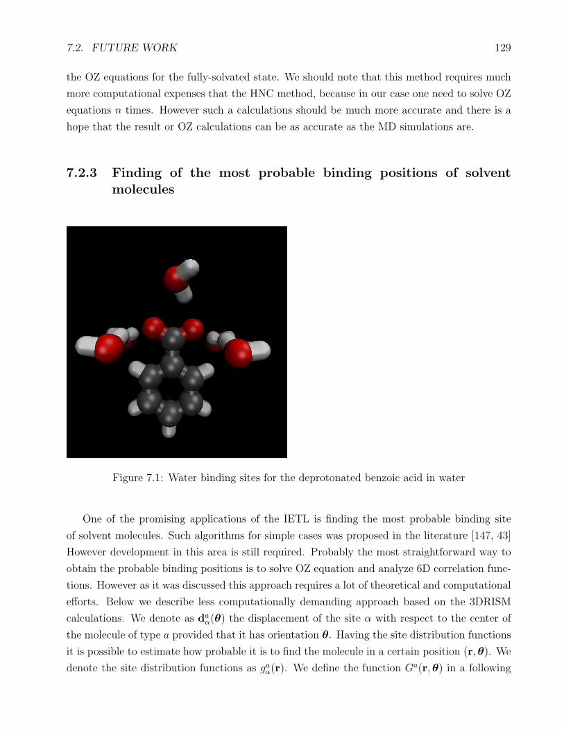
7.2. FUTURE WORK 129
the OZ equations for the fully-solvated state. We should note that this method requires much
more computational expenses that the HNC method, because in our case one need to solve OZ
equations n times. However such a calculations should be much more accurate and there is a
hope that the result or OZ calculations can be as accurate as the MD simulations are.
7.2.3 Finding of the most probable binding positions of solvent
molecules
Figure 7.1: Water binding sites for the deprotonated benzoic acid in water
One of the promising applications of the IETL is finding the most probable binding site
of solvent molecules. Such algorithms for simple cases was proposed in the literature [147, 43]
However development in this area is still required. Probably the most straightforward way to
obtain the probable binding positions is to solve OZ equation and analyze 6D correlation func-
tions. However as it was discussed this approach requires a lot of theoretical and computational
efforts. Below we describe less computationally demanding approach based on the 3DRISM
calculations. We denote as daα(θ) the displacement of the site α with respect to the center of
the molecule of type a provided that it has orientation θ. Having the site distribution functions
it is possible to estimate how probable it is to find the molecule in a certain position (r,θ). We
denote the site distribution functions as gaα(r). We define the function Ga(r,θ) in a following

130 CHAPTER 7. CONCLUSIONS AND FURTHER WORK
Figure 7.2: Water binding sites for the α-cyclodextrin in water
way:
Ga(r,θ) =
(Ka∏
α
gaα(r+ daα(θ))
)1/Ka
(7.9)
where Ka is the number of sites in the molecule a. The functions gaα are proportional to the
probability to find the site α in a certain position. The function Ga(r,θ) is proportional to the
probability to find the molecule a in a certain position (r,θ). We define the functions Gamax,
Θamax in a following way:
Gamax(r) = max
θGa(r,θ) (7.10)
Θamax(r) = argmaxθG
a(r,θ) (7.11)
The function Θamax(r) defines the most probable orientation of the molecule at the point r and
the function Gamax(r) is proportional to the maximal probability to find the molecule in the
point r . If we choose a certain threshold Gtres we can visualize the molecules in the positions
r1, . . . , rn such that Gamax(ri) > Gtres. The orientation of the visualized molecule is defined
by the function Θa(ri). To achieve a better visual effect it is reasonable to visualize only
one of the overlapping molecules in neighboring position, namely the molecule which have the
maximum value of Gmax(r) among all of the overlapping molecules. This method for visualizing
the binding sites was implemented as a plug-in for the Visual Molecular Dynamics program
[148]. This plug-in is an open-source program and is available for the online download [149]. To
illustrate the possibilities of the algorithm we performed the water binding site search for the
benzoic acid in a deprotonated state (CH5COO−). The results of the calculations are presented
in Figure 7.1. We see that the hydrogen atoms of water are oriented towards the negatively
7.3. CONCLUDING REMARKS 131
charged oxygens of COO− group which matches both: the common sense and the intuition. In
Figure 7.2 is presented the result of the water binding site calculations for α-cyclodextrin.
It is necessary to remind that RISM and 3DRISM models give a reasonably accurate descrip-
tion of small-molecule solvents. Due to this fact it is reasonable to assume that the described
above method for finding binding sites also works well only for small molecular solvents. Of
course for the solvents with larger molecules it is possible to use the 6D OZ equations which
immediately give the Ga(r,θ) functions. However, there are an alternative method. We can di-
vide a big solvent molecule into several fragments, for each of the fragments solve the 3DRISM
equations and calculate the Ga(r,θ) functions. Let Da(θ) be the displacement of the fragment
a with respect to the center of the solvent molecule in orientation θ. We define the function
G(r,θ) in a following way:
G(r,θ) =
(M∏
a=1
Gaα(r+Da(θ))
)1/M
(7.12)
where M is the number of fragments in the solvent molecule. The function G(r,θ) is pro-
portional to the probability to find a solvent molecule in the position (r,θ). Similarly as it
was done for Ga(r,θ) function we can find and visualize the most probable positions of big
solvent molecules. Of course this method is less accurate than the methods based on the OZ
equitations. However it is much simpler from the computational point of view and we think it
can be useful for practical applications.
7.3 Concluding remarks
Summarizing the current work and the future plans we can say that for a moment IETL is a
promising method which in principle in many cases can substitute computationally expansive
MD and MC simulations. In our work and in works of other researchers it was shown that
the integral equation theory can be of use for the accurate solvation free energy calculation[64,
65, 73, 66], predicting the self-assembling behavior[39] and many other applications[129, 150,
151]. From the other hand despite its potential the theory still is not widely used in practical
applications. This can be explained by the lack of developed theoretical and computational
methods. We mentioned three ways for future development of the theory and computational
methods, which are development of the universal six-dimensional OZ equation solver, search for
new closures and bridge functionals, developing new solvent binding methods. However there
are plenty other ways for development, which include for example the theory for confined and
non-uniform liquids, non-equilibrium density functional theory, theory for flexible molecules
etc. We hope that rapid development of the integral equation theory of liquids will result

132 CHAPTER 7. CONCLUSIONS AND FURTHER WORK
in a nearliest future in powerful methods which can be of use in variety of applications in
computational chemistry.
Appendix A
Low rank representation of
multidimensional functions
In this appendix the low-rank format for representation of multidimensional functions is de-
scribed. The low-rank format is quite general and is not necessarily be used for the repre-
sentation of the six-dimensional correlation functions which appear in the integral equation
theory of liquids. However, in this section we discuss the complexity of those operations with
the multidimensional functions in the low-rank format which are particularly relevant to the
numerical solution of the system of six-dimensional MOZ equations.
Low rank format
The idea of the low-rank format is to use different angle-grid resolutions at different distances to
the solute molecule. There are different ways to do that but the common idea may be illustrated
on the simple example and then generalized to more complicated systems. Let us consider a
simplified case when the correlation functions depend only on two variables: distance between
the molecules r and angle between the molecules θ. Such system for example describes the
interaction of the ball solute with the diatomic solvent. The function f(r, θ) can be represented
in a low-rank format. At the large distances all the functions in the OZ and closure equations
are smooth and tend to zero. This means, that at large distances one needs smaller number
of the basis functions to represent the initial function f(r, θ). This can be rewritten in such a
way: for each point r there is a rank M(r), which decays at large distances:
f(r, θ) =
M(r)∑
m=1
fm(r)φm(θ) (A.1)
where φm(θ) are some basis functions, M(r) ∈ N and M(r) → 0 when r → ∞.
133
134APPENDIX A. LOWRANKREPRESENTATIONOFMULTIDIMENSIONAL FUNCTIONS
Operation in the low rank format
Operations which we need to perform with the functions are:
• Converting to the low-rank format
• Reconstructing the function from the low-rank format
• Multiplication of the functions
• Calculation of the convolutions
Converting a function to the low rank format
To represent a function in the format (A.1) one needs to calculate the function only in certain
number of points. Let at the distance r the rank is M(r). We calculate the values of the
function f at the points (r, θn) where n = 1 . . .M(r). Using representation (A.1) we have:
f(r, θ1) =
M(r)∑
m=1
fm(r)φm(θ1)
. . .
f(r, θM(r)) =
M(r)∑
m=1
fm(r)φm(θM(r))
(A.2)
This is the system of linear equations with respect to the unknown coefficients f r1 . . . f
rM(r).
The matrix of the system Φ is the following:
Φ =
φ1(θ1) . . . φM(r)(θ1)...
. . ....
φ1(θM(r)) . . . φM(r)(θM(r))
(A.3)
We use the following definitions:
b = (f(r, θ1), . . . , f(r, θM(r))T , (A.4)
f = (f1(r), . . . , fM(r)(r))T (A.5)
Then the system (A.2) can be rewritten in the matrix notation:
Φf = b (A.6)
The coefficients f1, . . . , fM(r) can be found as
f = Φ−1b (A.7)
135
Because the matrix Φ consists of the values of the basis functions in the certain points
θ1, . . . , θM(r) the inverse matrix Φ−1 can be pre-computed before the calculations start, and
thus the calculation of the coefficients f at the point r will need M(r)2 operations. If the
distance r is discretized on the grid with N grid points, the total cost of the decomposition the
function f(r, θ) to the format (A.1) is∑N
n=1 M(rn)2 operations and only
∑Nn=1 M(r) function
calculations.
Reconstruction of the function from the low-rank format
To reconstruct the function from the low-rank format we should be able having the represen-
tation (A.1) to calculate the value of the function at any given point (r, θ). To do this, one
can simply use the formula (A.1). The computational cost of the calculation the value of the
function at the point (r, θ) is M(r) operations.
Multiplication in the low-rank format
Let we have two functions in the format (A.1):
f(r, θ) =
M1(r)∑
m1=1
fm1(r)φm1(θ)
g(r, θ) =
M2(r)∑
m2=1
gm2(r)φm2(θ)
(A.8)
We may formally multiply the representations:
f(r, θ)g(r, θ) =
M1(r)∑
m1=1
M2(r)∑
m2=1
fm1(r)gm2(r)φm1(θ)φm2(θ) (A.9)
Now we need to convert the product to the format (A.1). To do this we can find the
representation of the products φm1(θ)φm2(θ) in the following form:
φm1(θ)φm2(θ) =
M3∑
m3=1
am1m2m3φm3(θ) (A.10)
If such representation is known then the product (A.9) can be written as follows:
f(r, θ)g(r, θ) =
M3∑
m3=1
M1(r)∑
m1=1
M2(r)∑
m2=1
am1m2m3fm1(r)gm2(r)
· φm3(θ) (A.11)
which gives the representation in the format (A.1):
f(r, θ)g(r, θ) =
M3∑
m3=1
Pm3(r)φm3(θ) (A.12)

136APPENDIX A. LOWRANKREPRESENTATIONOFMULTIDIMENSIONAL FUNCTIONS
where Pm3(r) =∑M1(r)
m1=1
∑M2(r)m2=1 am1m2m3fm1(r)gm2(r)
This method needs M3 ·M1(r) ·M2(r) operations to calculate the coefficients at the certain
distance r, and thus∑N
n=1 M3 ·M1(rn) ·M2(rn) operation in total to perform the multiplication.
However, there is a simpler method. We assume, that the rank of the product at the point
r is fixed, and denote it M3(r). In that case we can just calculate for each r the values of the
product at the points (r, θ1), . . . , (r, θM3(r)) and reconstruct the coefficients using the formula
(A.7).
The computational cost of calculating of the product coefficients at the distance r includes:
• calculating the values of the functions f(r, θ) and g(r, θ) and their product at the points
(r, θ1), . . . , (r, θM3(r)). This takes M3(r)(M1(r) +M2(r) + 1) operations
• reconstructing the coefficients of the product from the values at the points (r, θ1), . . . , (r, θM3(r)).
This takes M3(r)2 operations.
So, in total, if there are N discretization points of the grid in distance direction the computa-
tional cost is∑N
n=1 M3(r)(M1(r) +M2(r) +M3(r) + 1) operations.
Calculating a convolution
Let we have two functions in the format (A.1):
f(r, θ) =∑M1(r)
m1=1 fm1(r)φm1(θ)
g(r, θ) =∑M2(r)
m2=1 gm2(r)φm2(θ)(A.13)
We may formally calculate the convolution of these functions:
∫ ∫
f(r′ − r, θ′ − θ)g(r′, θ′)dr′dθ′ =
M1(r)∑
m1=1
M2(r)∑
m2=1
∫
fm1(r′ − r)gm2(r
′)dr′∫
φm1(θ′ − θ)φm2(θ
′)dθ′
(A.14)
Now we need to convert the convolution to the format (A.1). To do this we can find the
representation of the convolutions∫φm1(θ
′ − θ)φm2(θ′)dθ′ in the following form:
∫
φm1(θ′ − θ)φm2(θ
′)dθ′ =
M3∑
m3=1
bm1m2m3φm3(θ) (A.15)
If such a representation is known, the convolution (A.14) can be written as follows:
∫
f(r′ − r, θ′ − θ)g(r′, θ′)dr′dθ′ =
M3∑
m3=1
M1(r)∑
m1=1
M2(r)∑
m2=1
bm1m2m3
∫
fm1(r′ − r)gm2(r
′)dr′
· φm3(θ)
(A.16)
137
which gives the representation in the format (A.1):
f(r, θ)g(r, θ) =
M3∑
m3=1
Cm3(r)φm3(θ) (A.17)
where Cm3(r) =∑M1(r)
m1=1
∑M2(r)m2=1 bm1m2m3
∫fm1(r
′ − r)gm2(r′)dr′
This method needs to calculate convolutions of each pair of functions fm1(r) and gm2(r).
Each convolution takes const · N log(N) operations. Because the convolution is a non-local
operation, the procedure will need const ·max(M1(r))max(M2(r))N log(N) operations.
Fourier low-rank representation
In the previous sections we did not make any assumptions about the basis set φ1(θ), . . . , φM(r)(θ).
However, by using the special basis sets one can essentially reduce the computational expanses.
One of the convenient basis sets for our calculations is the Fourier basis φm(θ) = e−imθ. How-
ever, for this format it is more natural to let m be negative: m ∈ Z So, finally the Fourier
analogue of the format (A.1) is the following:
f(r, θ) =
M(r)/2∑
−M(r)/2
fm(r)e−imθ (A.18)
The format is convenient by two reasons:
• Firstly, at large distances the angular component of the functions in the Ornstein-Zernike
equation can be approximated by the sin/cos functions with the high accuracy.
• Secondly, the Fourier basis essentially simplifies the calculations and allows us in many
cases to use the efficient FFT algorithm.
Below we will see how the Fourier basis can simplify the basic operations.
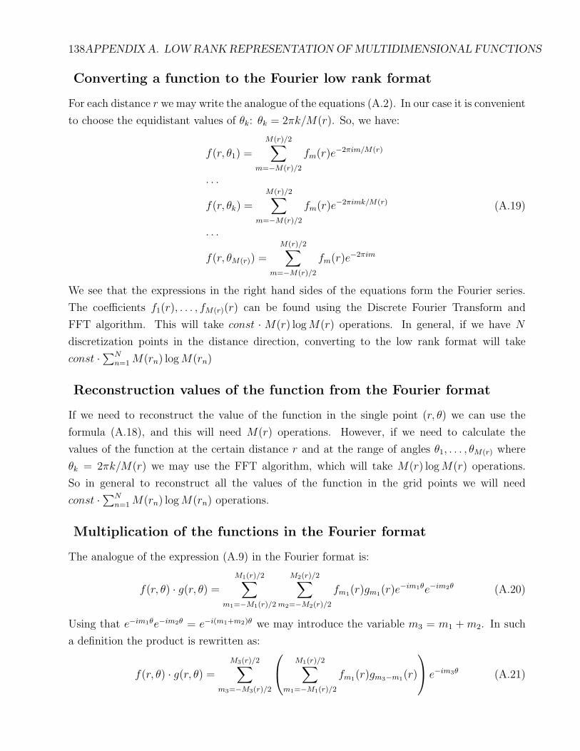
138APPENDIX A. LOWRANKREPRESENTATIONOFMULTIDIMENSIONAL FUNCTIONS
Converting a function to the Fourier low rank format
For each distance r we may write the analogue of the equations (A.2). In our case it is convenient
to choose the equidistant values of θk: θk = 2πk/M(r). So, we have:
f(r, θ1) =
M(r)/2∑
m=−M(r)/2
fm(r)e−2πim/M(r)
. . .
f(r, θk) =
M(r)/2∑
m=−M(r)/2
fm(r)e−2πimk/M(r)
. . .
f(r, θM(r)) =
M(r)/2∑
m=−M(r)/2
fm(r)e−2πim
(A.19)
We see that the expressions in the right hand sides of the equations form the Fourier series.
The coefficients f1(r), . . . , fM(r)(r) can be found using the Discrete Fourier Transform and
FFT algorithm. This will take const · M(r) logM(r) operations. In general, if we have N
discretization points in the distance direction, converting to the low rank format will take
const ·∑Nn=1 M(rn) logM(rn)
Reconstruction values of the function from the Fourier format
If we need to reconstruct the value of the function in the single point (r, θ) we can use the
formula (A.18), and this will need M(r) operations. However, if we need to calculate the
values of the function at the certain distance r and at the range of angles θ1, . . . , θM(r) where
θk = 2πk/M(r) we may use the FFT algorithm, which will take M(r) logM(r) operations.
So in general to reconstruct all the values of the function in the grid points we will need
const ·∑Nn=1 M(rn) logM(rn) operations.
Multiplication of the functions in the Fourier format
The analogue of the expression (A.9) in the Fourier format is:
f(r, θ) · g(r, θ) =M1(r)/2∑
m1=−M1(r)/2
M2(r)/2∑
m2=−M2(r)/2
fm1(r)gm1(r)e−im1θe−im2θ (A.20)
Using that e−im1θe−im2θ = e−i(m1+m2)θ we may introduce the variable m3 = m1 +m2. In such
a definition the product is rewritten as:
f(r, θ) · g(r, θ) =M3(r)/2∑
m3=−M3(r)/2
M1(r)/2∑
m1=−M1(r)/2
fm1(r)gm3−m1(r)
e−im3θ (A.21)
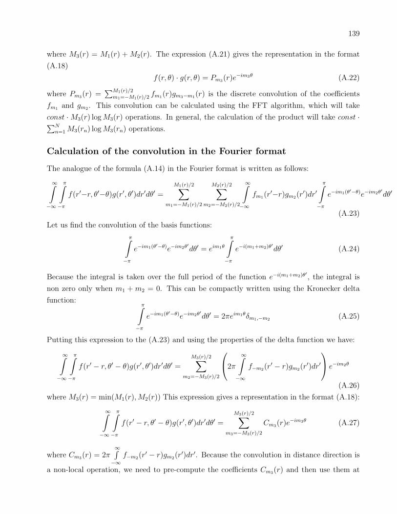
139
where M3(r) = M1(r) +M2(r). The expression (A.21) gives the representation in the format
(A.18)
f(r, θ) · g(r, θ) = Pm3(r)e−im3θ (A.22)
where Pm3(r) =∑M1(r)/2
m1=−M1(r)/2fm1(r)gm3−m1(r) is the discrete convolution of the coefficients
fm1 and gm2 . This convolution can be calculated using the FFT algorithm, which will take
const ·M3(r) logM3(r) operations. In general, the calculation of the product will take const ·∑N
n=1 M3(rn) logM3(rn) operations.
Calculation of the convolution in the Fourier format
The analogue of the formula (A.14) in the Fourier format is written as follows:
∞∫
−∞
π∫
−π
f(r′−r, θ′−θ)g(r′, θ′)dr′dθ′ =
M1(r)/2∑
m1=−M1(r)/2
M2(r)/2∑
m2=−M2(r)/2
∞∫
−∞
fm1(r′−r)gm2(r
′)dr′π∫
−π
e−im1(θ′−θ)e−im2θ′dθ′
(A.23)
Let us find the convolution of the basis functions:
π∫
−π
e−im1(θ′−θ)e−im2θ′dθ′ = eim1θ
π∫
−π
e−i(m1+m2)θ′dθ′ (A.24)
Because the integral is taken over the full period of the function e−i(m1+m2)θ′ , the integral is
non zero only when m1 + m2 = 0. This can be compactly written using the Kronecker delta
function:π∫
−π
e−im1(θ′−θ)e−im2θ′dθ′ = 2πeim1θδm1,−m2 (A.25)
Putting this expression to the (A.23) and using the properties of the delta function we have:
∞∫
−∞
π∫
−π
f(r′ − r, θ′ − θ)g(r′, θ′)dr′dθ′ =
M3(r)/2∑
m2=−M3(r)/2
2π
∞∫
−∞
f−m2(r′ − r)gm2(r
′)dr′
e−im2θ
(A.26)
where M3(r) = min(M1(r),M2(r)) This expression gives a representation in the format (A.18):
∞∫
−∞
π∫
−π
f(r′ − r, θ′ − θ)g(r′, θ′)dr′dθ′ =
M3(r)/2∑
m3=−M3(r)/2
Cm3(r)e−im3θ (A.27)
where Cm3(r) = 2π∞∫
−∞f−m2(r
′ − r)gm2(r′)dr′. Because the convolution in distance direction is
a non-local operation, we need to pre-compute the coefficients Cm3(r) and then use them at

140APPENDIX A. LOWRANKREPRESENTATIONOFMULTIDIMENSIONAL FUNCTIONS
any distance r. However, we need to calculate the convolutions only of the selected pairs of
the functions fm1(r) and gm2(r), namely of such of them that m1 = −m2. This will give only
M3 = min(maxr M1(r),maxr M2(r)) convolution calculations. Moreover, because the ranks
M1(r) and M2(r) decay at the large distances, that means that the support of the the functions
fm1(r) and gm2(r) will decay with the growth of the coefficients m1 and m2. And the functions
with the smaller support need smaller number of discretization points. We denote N(f(r)) the
number of points which is needed to descretize the function f(r). Then the total computational
cost to calculate the convolution is const ·∑M3/2
m3=−M3/2Nm3 logNm3 , where Nm3 = N(f−m3(r))+
N(gm3(r))
Bibliography
[1] C. A. Reynolds, P. M. King, and W. G. Richards. Free-energy calculations in molecular
biophysics. Molecular Physics, 76(2):251–275, June 1992.
[2] P. Kollman. Free-energy calculations - applications to chemical and biochemical phenom-
ena. Chemical Reviews, 93(7):2395–2417, November 1993.
[3] G.L. Perlovich and A. Bauer-Brandl. Solvation of drugs as a key for understanding parti-
tioning and passive transport exemplified by nsaids. Current Drug Delivery, 1(3):213–226,
July 2004.
[4] G. L. Perlovich, T. V. Volkova, and A. Bauer-Brandl. Towards an understanding of
the molecular mechanism of solvation of drug molecules: A thermodynamic approach by
crystal lattice energy, sublimation, and solubility exemplified by paracetamol, acetanilide,
and phenacetin. Journal of Pharmaceutical Sciences, 95(10):2158–2169, October 2006.
[5] G. L. Perlovich, L. K. Hansen, T. V. Volkova, S. Mirza, A. N. Manin, and A. Bauer-
Brandl. Thermodynamic and structural aspects of hydrated and unhydrated phases of
4-hydroxybenzamide. Crystal Growth & Design, 7(12):2643–2648, December 2007.
[6] L. D. Hughes, D. S. Palmer, F. Nigsch, and J. B. O. Mitchell. Why are some properties
more difficult to predict than others? a study of qspr models of solubility, melting point,
and log p. Journal of Chemical Information and Modeling, 48(1):220–232, January 2008.
[7] D. S. Palmer, A. Llinas, I. Morao, G. M. Day, J. M. Goodman, R. C. Glen, and J. B. O.
Mitchell. Predicting intrinsic aqueous solubility by a thermodynamic cycle. Molecular
Pharmaceutics, 5(2):266–279, March 2008.
[8] W. L. Jorgensen and J. TiradoRives. Free energies of hydration for organic molecules
from monte carlo simulations. Perspectives in Drug Discovery and Design, 3:123–138,
1995.
[9] N. Matubayasi and M. Nakahara. Theory of solutions in the energetic representation. i.
formulation. Journal of Chemical Physics, 113(15):6070–6081, October 2000.
141

142 BIBLIOGRAPHY
[10] N. Matubayasi and M. Nakahara. An approach to the solvation free energy in terms of
the distribution functions of the solute-solvent interaction energy. Journal of Molecular
Liquids, 119(1-3):23–29, May 2005.
[11] M. R. Shirts and V. S. Pande. Solvation free energies of amino acid side chain
analogs for common molecular mechanics water models. Journal of Chemical Physics,
122(13):134508, April 2005.
[12] N. Matubayasi. Free-energy analysis of solvation with the method of energy representa-
tion. Frontiers in Bioscience, 14:3536–3549, January 2009.
[13] J. L. Knight and C. L. Brooks. lambda-dynamics free energy simulation methods. Journal
of Computational Chemistry, 30(11):1692–1700, August 2009.
[14] J. Tomasi and M. Persico. Molecular-interactions in solution - an overview of methods
based on continuous distributions of the solvent. Chemical Reviews, 94(7):2027–2094,
November 1994.
[15] B. Roux and T. Simonson. Implicit solvent models. Biophysical Chemistry, 78(1-2):1–20,
April 1999.
[16] D. Bashford and D. A. Case. Generalized born models of macromolecular solvation effects.
Annual Review of Physical Chemistry, 51:129–152, 2000.
[17] J. Tomasi, B. Mennucci, and R. Cammi. Quantum mechanical continuum solvation
models. Chemical Reviews, 105(8):2999–3094, August 2005.
[18] M. B. Ulmschneider, J. P. Ulmschneider, M. S. P. Sansom, and A. Di Nola. A generalized
born implicit-membrane representation compared to experimental insertion free energies.
Biophysical Journal, 92(7):2338–2349, April 2007.
[19] A. V. Marenich, C. J. Cramer, and D. G. Truhlar. Performance of sm6, sm8, and smd on
the sampl1 test set for the prediction of small-molecule solvation free energies. Journal
of Physical Chemistry B, 113(14):4538–4543, March 2009.
[20] A. Klamt, F. Eckert, and M. Diedenhofen. Prediction of the free energy of hydra-
tion of a challenging set of pesticide-like compounds. Journal of Physical Chemistry
B, 113(14):4508–4510, March 2009.
[21] T. Sulea, D. Wanapun, S. Dennis, and E. O. Purisima. Prediction of sampl-1 hydra-
tion free energies using a continuum electrostatics-dispersion model. Journal of Physical
Chemistry B, 113(14):4511–4520, March 2009.
BIBLIOGRAPHY 143
[22] P. A. Monson and G. P. Morriss. Recent progress in the statistical-mechanics of interaction
site fluids. Advances in Chemical Physics, 77:451–550, 1990.
[23] J.-P. Hansen and I. R. McDonald. Theory of Simple Liquids, 3rd ed. Academic Press,
London, 1991.
[24] F. Hirata, editor. Molecular theory of solvation. Kluwer Academic Publishers, Dordrecht,
Netherlands, 2003.
[25] L. Blum and A. J. Torruella. Invariant expansion for two-body correlations: Thermo-
dynamic functions, scattering, and the Ornstein-Zernike equation. Journal of Chemical
Physics, 56(1):303–310, 1972.
[26] K. Amano and M. Kinoshita. Entropic insertion of a big sphere into a cylindrical vessel.
Chemical Physics Letters, 488(1-3):1–6, March 2010.
[27] D. Chandler and H. C. Andersen. Optimized cluster expansions for classical fluids. 2.
Theory of molecular liquids. Journal of Chemical Physics, 57(5):1930–1937, 1972.
[28] F. Hirata, B. M. Pettitt, and P. J. Rossky. Application of an extended RISM equation
to dipolar and quadrupolar fluids. Journal of Chemical Physics, 77(1):509–520, 1982.
[29] B. M. Pettitt and P. J. Rossky. Integral-equation predictions of liquid-state structure for
waterlike intermolecular potentials. Journal of Chemical Physics, 77(3):1451–1457, 1982.
[30] M. Kinoshita, Y. Okamoto, and F. Hirata. Calculation of solvation free energy using RISM
theory for peptide in salt solution. Journal of Computational Chemistry, 19(15):1724–
1735, November 1998.
[31] M. Kinoshita, Y. Okamoto, and F. Hirata. First-principle determination of peptide con-
formations in solvents: Combination of monte carlo simulated annealing and rism theory.
Journal of the American Chemical Society, 120(8):1855–1863, March 1998.
[32] M. Kinoshita, Y. Okamoto, and F. Hirata. Analysis on conformational stability of c-
peptide of ribonuclease a in water using the reference interaction site model theory and
monte carlo simulated annealing. Journal of Chemical Physics, 110(8):4090–4100, Febru-
ary 1999.
[33] T. Imai, M. Kinoshita, and F. Hirata. Salt effect on stability and solvation structure
of peptide: An integral equation study. Bulletin of the Chemical Society of Japan,
73(5):1113–1122, May 2000.
144 BIBLIOGRAPHY
[34] T. Imai, R. Hiraoka, A. Kovalenko, and F. Hirata. Water molecules in a protein cavity
detected by a statistical-mechanical theory. Journal of the American Chemical Society,
127(44):15334–15335, November 2005.
[35] N. Yoshida, S. Phongphanphanee, Y. Maruyama, T. Imai, and F. Hirata. Selective ion-
binding by protein probed with the 3d-rism theory. Journal of the American Chemical
Society, 128(37):12042–12043, September 2006.
[36] N. Yoshida, S. Phongphanphanee, and F. Hirata. Selective Ion Binding by Protein Probed
with the Statistical Mechanical Integral Equation Theory. Journal of Physical Chemistry
B, 111(17):4588–4595, 2007.
[37] G.N. Chuev, M.V. Fedorov, and J. Crain. Improved estimates for hydration free energy
obtained by the reference interaction site model. Chemical Physics Letters, 448(4-6):198–
202, 2007.
[38] M. V. Fedorov and A. A. Kornyshev. Unravelling the solvent response to neutral and
charged solutes. Molecular Physics, 105(1):1–16, January 2007.
[39] G. N. Chuev and M. V. Fedorov. Reference interaction site model study of self-aggregating
cyanine dyes. The Journal of Chemical Physics, 131:074503, 2009.
[40] T. Imai, Y. Harano, M. Kinoshita, A. Kovalenko, and F. Hirata. Theoretical analysis on
changes in thermodynamic quantities upon protein folding: Essential role of hydration.
Journal of Chemical Physics, 126(22):225102, June 2007.
[41] T. Imai, S. Ohyama, A. Kovalenko, and F. Hirata. Theoretical study of the partial molar
volume change associated with the pressure-induced structural transition of ubiquitin.
Protein Science, 16(9):1927–1933, September 2007.
[42] D. Yokogawa, H. Sato, T. Imai, and S. Sakaki. A highly parallelizable integral equation
theory for three dimensional solvent distribution function: Application to biomolecules.
Journal of Chemical Physics, 130(6):064111, February 2009.
[43] T. Imai, K. Oda, A. Kovalenko, F. Hirata, and A. Kidera. Ligand mapping on pro-
tein surfaces by the 3d-rism theory: Toward computational fragment-based drug design.
Journal of the American Chemical Society, 131(34):12430–12440, September 2009.
[44] Y. Kiyota, R. Hiraoka, N. Yoshida, Y. Maruyama, I. Imai, and F. Hirata. Theoretical
study of co escaping pathway in myoglobin with the 3d-rism theory. Journal of the
American Chemical Society, 131(11):3852–3853, March 2009.
BIBLIOGRAPHY 145
[45] K. Nishiyama, T. Yamaguchi, and F. Hirata. Solvation dynamics in polar solvents studied
by means of rism/mode-coupling theory. Journal of Physical Chemistry B, 113(9):2800–
2804, March 2009.
[46] D. Frenkel and B. Smit. Understanding molecular simulation. Academic Press, 2002.
[47] M. V. Fedorov, J. M. Goodman, and S. Schumm. The effect of sodium chloride on
poly-l-glutamate conformation. Chemical Communications, (8):896–898, 2009.
[48] M. V. Fedorov, J. M. Goodman, and S. Schumm. To switch or not to switch: The effects of
potassium and sodium ions on alpha-poly-l-glutamate conformations in aqueous solutions.
Journal of the American Chemical Society, 131(31):10854–10856, August 2009.
[49] Benedetta Mennucci and Roberto Cammi, editors. Continuum Solvation Models in Chem-
ical Physics. Wiley, Chippenham, Wiltshire, UK, 2007.
[50] J.-P. Hansen and I. R. McDonald. Theory of Simple Liquids, 4th ed. Elsevier Academic
Press, Amsterdam, The Netherlands, 2000.
[51] E. Meeron. Series expansion of distribution functions in multicomponent fluid systems.
Journal of Chemical Physics, 27(6):1238–1246, 1957.
[52] S. J. Singer and D. Chandler. Free-energy functions in the extended rism approximation.
Molecular Physics, 55(3):621–625, 1985.
[53] L. Gendre, R. Ramirez, and D. Borgis. Classical density functional theory of solvation
in molecular solvents: Angular grid implementation. Chemical Physics Letters, 474(4-
6):366–370, June 2009.
[54] R. Ramirez, R. Gebauer, M. Mareschal, and D. Borgis. Density functional theory of solva-
tion in a polar solvent: Extracting the functional from homogeneous solvent simulations.
Physical Review E, 66(3):031206, September 2002.
[55] T. Urbic, V. Vlachy, Y. V. Kalyuzhnyi, and K. A. Dill. Orientation-dependent integral
equation theory for a two-dimensional model of water. Journal of Chemical Physics,
118(12):5516–5525, March 2003.
[56] M. V. Fedorov, H. J. Flad, G. N. Chuev, L. Grasedyck, and B. N. Khoromskij. A
structured low-rank wavelet solver for the Ornstein-Zernike integral equation. Computing,
80(1):47–73, May 2007.

146 BIBLIOGRAPHY
[57] S. Ten-no, F. Hirata, and S. Kato. A hybrid approach for the solvent effect on the
electronic-structure of a solute based on the rism and hartree-fock equations. Chemical
Physics Letters, 214(3-4):391–396, November 1993.
[58] S. Ten-no, F. Hirata, and S. Kato. Reference interaction site model self-consistent-field
study for solvation effect on carbonyl-compounds in aqueous-solution. Journal of Chem-
ical Physics, 100(10):7443–7453, May 1994.
[59] H. Sato, F. Hirata, and S. Kato. Analytical energy gradient for the reference inter-
action site model multiconfigurational self-consistent-field method: Application to 1,2-
difluoroethylene in aqueous solution. Journal of Chemical Physics, 105(4):1546–1551,
July 1996.
[60] D. Yokogawa, H. Sato, and S. Sakaki. New generation of the reference interaction site
model self-consistent field method: Introduction of spatial electron density distribution
to the solvation theory. Journal of Chemical Physics, 126(24):244504, June 2007.
[61] D. Yokogawa, H. Sato, and S. Sakaki. The position of water molecules in bacteri-
orhodopsin: A three-dimensional distribution function study. Journal of Molecular Liq-
uids, 147(1-2):112–116, July 2009.
[62] S. Ten-no. Free energy of solvation for the reference interaction site model: Critical
comparison of expressions. Journal of Chemical Physics, 115(8):3724–3731, August 2001.
[63] Y. Karino, M. V. Fedorov, and N. Matubayasi. End-point calculation of solvation free
energy of amino-acid analogs by molecular theories of solution. Chemical Physics Letters,
496(4-6):351–355, August 2010.
[64] D. S. Palmer, V. P. Sergiievskyi, F. Jensen, and M. V. Fedorov. Accurate calculations
of the hydration free energies of druglike molecules using the reference interaction site
model. Journal of Chemical Physics, 133(4):044104, July 2010.
[65] E. L. Ratkova, G. N. Chuev, V. P. Sergiievskyi, and M. V. Fedorov. An accurate prediction
of hydration free energies by combination of molecular integral equations theory with
structural descriptors. Journal of Physical Chemistry B, 114(37):12068–12079, 2010.
[66] E. L. Ratkova and M. V. Fedorov. Combination of rism and cheminformatics for efficient
predictions of hydration free energy of polyfragment molecules: Application to a set of
organic pollutants. Journal of Chemical Theory and Computation, 7(5):1450–1457, 2011.

BIBLIOGRAPHY 147
[67] V. P. Sergiievskyi. Model for calculating the free energy of hydration of bioactive com-
pounds based on integral equations of the theory of liquids. Russian Journal of Physical
Chemistry B, 5(2):326–331, 2011.
[68] D. Chandler, J. D. Mccoy, and S. J. Singer. Density functional theory of nonuniform
polyatomic systems. 1. General formulation. Journal of Chemical Physics, 85(10):5971–
5976, 1986.
[69] D. Beglov and B. Roux. Numerical-solution of the hypernetted-chain equation for a solute
of arbitrary geometry in 3 dimensions. Journal of Chemical Physics, 103(1):360–364, July
1995.
[70] T. Imai. Molecular theory of partial molar volume and its applications to biomolecular
systems. Condensed Matter Physics, 10(3):343–361, 2007.
[71] T. Luchko, S. Gusarov, D. R. Roe, C. Simmerling, D. A. Case, J. Tuszynski, and A. Ko-
valenko. Three-dimensional molecular theory of solvation coupled with molecular dy-
namics in amber. Journal of Chemical Theory and Computation, 6(3):607–624, March
2010.
[72] M. C. Stumpe, N. Blinov, D. Wishart, A. Kovalenko, and V. S. Pande. Calculation of local
water densities in biological systems: A comparison of molecular dynamics simulations
and the 3d-rism-kh molecular theory of solvation. Journal of Physical Chemistry B,
115(2):319–328, January 2011.
[73] D. S. Palmer, G. N. Chuev, E. L. Ratkova, and M. V. Fedorov. In silico screening of
bioactive and biomimetic solutes by integral equation theory. Current Pharmaceutical
Design, 17(17):1695–1708, 2011.
[74] A. I. Frolov, E. L. Ratkova, D. S. Palmer, and M. V. Fedorov. Hydration thermodynamics
using the reference interaction site model: Speed or accuracy? The Journal of Physical
Chemistry B, 115(19):6011–6022, 2011.
[75] G. Zerah. An efficient newtons method for the numerical-solution of fluid integral-
equations. Journal of Computational Physics, 61(2):280–285, 1985.
[76] Michael J. Booth, A.G. Schlijper, L.E. Scales, and A.D.J. Haymet. Efficient solution
of liquid state integral equations using the newton–gmres algorithm. Computer Physics
Communications, 119:122–134, 1999.

148 BIBLIOGRAPHY
[77] A. Kovalenko, S. Ten-No, and F. Hirata. Solution of three-dimensional reference interac-
tion site model and hypernetted chain equations for simple point charge water by modified
method of direct inversion in iterative subspace. Journal of Computational Chemistry,
20(9):928–936, July 1999.
[78] M. Kawata, C. M. Cortis, and R. A. Friesner. Efficient recursive implementation of
the modified broyden method and the direct inversion in the iterative subspace method:
Acceleration of self-consistent calculations. Journal of Chemical Physics, 108(11):4426–
4438, March 1998.
[79] H.H.H. Homeier, S. Rast, and H. Krienke. Iterative solution of the Ornstein-Zernike equa-
tion with various closures using vector extrapolation. Computer Physics Communications,
92(2-3):188–202, 1995.
[80] M. J. Gillan. New method of solving the liquid structure integral-equations. Molecular
Physics, 38(6):1781–1794, 1979.
[81] S. Labik, A. Malijevsky, and P. Vonka. A rapidly convergent method of solving the
Ornstein-Zernike equation. Molecular Physics, 56(3):709–715, 1985.
[82] S. Woelki, H.H. Kohler, H. Krienke, and G. Schmeer. Improvements of DRISM calcula-
tions: symmetry reduction and hybrid algorithms. Physical Chemistry Chemical Physics,
10(6):898–910, 2008.
[83] G. N. Chuev and M. V. Fedorov. Wavelet algorithm for solving integral equations of
molecular liquids. a test for the reference interaction site model. Journal of Computational
Chemistry, 25(11):1369–1377, August 2004.
[84] G. N. Chuev and M. V. Fedorov. Wavelet treatment of structure and thermodynamics of
simple liquids. Journal of Chemical Physics, 120(3):1191–1196, January 2004.
[85] M. V. Fedorov and G. N. Chuev. Wavelet method for solving integral equations of simple
liquids. Journal of Molecular Liquids, 120(1–3):159–162, June 2005.
[86] C. T. Kelley and B. M. Pettitt. A fast solver for the Ornstein-Zernike equations. Journal
of Computational Physics, 197(2):491–501, JUL 2004.
[87] W. Hackbusch. Multi-grid methods and Applications. Springer-Verlag, Berlin, 1985.
[88] H. Y. Wang, W. Jiang, and Y. N. Wang. Implicit and electrostatic particle-in-cell/monte
carlo model in two-dimensional and axisymmetric geometry: I. analysis of numerical
techniques. Plasma Sources Science & Technology, 19(4):045023, August 2010.

BIBLIOGRAPHY 149
[89] M. Heiskanen, T. Torsti, M.J. Puska, and R.M. Nieminen. Multigrid method for electronic
structure calculations. Physical Review B, 63(24):245106, JUN 15 2001.
[90] W. Janke and T. Sauer. Multicanonical multigrid Monte-Carlo method. Physical Review
E, 49(4, Part B):3475–3479, APR 1994.
[91] F. Gygi and G. Galli. Real-space adaptive-coordinate electronic-structure calculations.
Physical Review B, 52(4):R2229–R2232, 1995.
[92] M. V. Fedorov and W. Hackbusch. A multigrid solver for the integral equations of the
theory of liquids. Preprint 88, Max-Planck-Institut fuer Mathematik in den Naturwis-
senschaften, 2008.
[93] J. P. Guthrie. A blind challenge for computational solvation free energies: Introduction
and overview. Journal of Physical Chemistry B, 113(14):4501–4507, April 2009.
[94] L. D. Landau and E. M. Lifshitz. Statistical Physics, Third Edition, Part 1: Volume 5
of Course of Theoretical Physics, volume 5. Butterworth-Heinemann, 3 edition, January
1980.
[95] V.I. Kalikmanov. Statistical physics of fluids: basic concepts and applications. Berlin;
New York: Springer, 2001.
[96] L. D. Landau and E. M. Lifshitz. Mechanics, Third Edition: Volume 1 of Course of
Theoretical Physics, volume 1. Butterworth-Heinemann, 3 edition, 1976.
[97] R.K. Pathria and Paul D. Beale. Statistical mechanics. 3rd. expanded ed. Boston, MA:
Academic Press. 744 p. , 2011.
[98] A letter from the late reverent mr. thomas bayes f.r.s to john canton, m.a. abd f.r.s,
http://www.york.ac.uk/depts/maths/histstat/letter.pdf.
[99] Lagrange multipliers. encyclopedia of mathematics., URL:
http://www.encyclopediaofmath.org/index.php?title=Lagrange multipliers.
[100] Eric W. Weisstein. Gaussian integral. from mathworld–a wolfram web resource.
http://mathworld.wolfram.com/gaussianintegral.html.
[101] V. M. Alekseev, V. M Tikhomirov, and S. V. Fomin. Optimal Control. New York :
Consultants Bureau, 1987.
[102] A. Ben-Naim. Molecular Theory of Solutions. Oxford University Press, USA, 2006.

150 BIBLIOGRAPHY
[103] J. K. Percus and G. J. Yevick. Analysis of classical statistical mechanics by means of
collective coordinates. Physical Review, 110(1):1–13, 1958.
[104] G. A. Martynov and G. N. Sarkisov. Exact equations and the theory of liquids .5.
Molecular Physics, 49(6):1495–1504, 1983.
[105] S. Labik, A. Malijevsky, and W. R. Smith. An accurate integral-equation for molecular
fluids .2. hard heteronuclear diatomics. Molecular Physics, 73(3):495–502, June 1991.
[106] H. C. Andersen. The structure of liquids. Annual Review of Physical Chemistry, 26:145–
166, 1975.
[107] V. N. Bondarev. Ising-like criticality derived from the theory of fluids. Physical Review
E, 77(5):050103, May 2008.
[108] V. P. Sergievskii and A. I. Frolov. Universal bridge functional for infinitely diluted so-
lutions: a case study for lennard-jones spheres of different diameter. Russian Journal of
Physical Chemistry A, 86(8):1254–1260, 2012. preprint: arXiv:1111.2257v1.
[109] S. Palmer, A. I. Frolov, E. L. Ratkova, and M. V. Fedorov. Towards a universal method
to calculate hydration free energies: a 3d reference interaction site model with partial
molar volume correction. Journal of Physics: Condensed Matter, 22(49):492101, 2010.
[110] J. G. Kirkwood. Statistical mechanics of fluid mixtures. Journal of Chemical Physics,
3:300–313, 1935.
[111] S. Ten-no and S. Iwata. On the connection between the reference interaction site model
integral equation theory and the partial wave expansion of the molecular Ornstein-Zernike
equation. Journal of Chemical Physics, 111(11):4865–4868, 1999.
[112] A. Kovalenko and F. Hirata. Hydration free energy of hydrophobic solutes studied by a
reference interaction site model with a repulsive bridge correction and a thermodynamic
perturbation method. Journal of Chemical Physics, 113:2793–2805, 2000.
[113] D. Chandler, Y. Singh, and D. M. Richardson. Excess electrons in simple fluids .1.
general equilibrium-theory for classical hard-sphere solvents. Journal of Chemical Physics,
81(4):1975–1982, 1984.
[114] V. P. Sergiievskyi, W. Hackbusch, and M. V. Fedorov. Multigrid solver for the reference
interaction site model of molecular liquids theory. Journal of Computational Chemistry,
32(9):1982–1992, 2011.

BIBLIOGRAPHY 151
[115] A. Kovalenko and F. Hirata. Potential of mean force between two molecular ions in
a polar molecular solvent: A study by the three-dimensional reference interaction site
model. Journal of Physical Chemistry B, 103:7942–7957, 1999.
[116] K. C. Ng. Hypernetted chain solutions for the classical one-component plasma up to
/gamma =7000. Journal of Chemical Physics, 61(7):2680–2689, 1974.
[117] Rism-mol solver: the program for fast and accurate rism solvation free energy calculations,
http://compchemmpi.wikispaces.com/RISM-MOL.
[118] W. L. Jorgensen and J. Tirado-Rives. Potential energy functions for atomic-level sim-
ulations of water and organic and biomolecular systems. Proceedings of the National
Academy of Sciences of the United States of America, 102(19):6665–6670, May 2005.
[119] W. L. Jorgensen and J. Tirado-Rives. Molecular modeling of organic and biomolecular
systems using boss and mcpro. Journal of Computational Chemistry, 26(16):1689–1700,
December 2005.
[120] D. Shivakumar, J. Williams, Y. J. Wu, W. Damm, J. Shelley, and W. Sherman. Prediction
of absolute solvation free energies using molecular dynamics free energy perturbation and
the opls force field. Journal of Chemical Theory and Computation, 6(5):1509–1519, May
2010.
[121] M. J. Frisch, G. W. Trucks, H. B. Schlegel, G. E. Scuseria, M. A. Robb, J. R. Cheese-
man, Montgomery, Jr., J. A., T. Vreven, K. N. Kudin, J. C. Burant, J. M. Millam,
S. S. Iyengar, J. Tomasi, V. Barone, B. Mennucci, M. Cossi, G. Scalmani, N. Rega,
G. A. Petersson, H. Nakatsuji, M. Hada, M. Ehara, K. Toyota, R. Fukuda, J. Hasegawa,
M. Ishida, T. Nakajima, Y. Honda, O. Kitao, H. Nakai, M. Klene, X. Li, J. E. Knox,
H. P. Hratchian, J. B. Cross, V. Bakken, C. Adamo, J. Jaramillo, R. Gomperts, R. E.
Stratmann, O. Yazyev, A. J. Austin, R. Cammi, C. Pomelli, J. W. Ochterski, P. Y. Ayala,
K. Morokuma, G. A. Voth, P. Salvador, J. J. Dannenberg, V. G. Zakrzewski, S. Dapprich,
A. D. Daniels, M. C. Strain, O. Farkas, D. K. Malick, A. D. Rabuck, K. Raghavachari,
J. B. Foresman, J. V. Ortiz, Q. Cui, A. G. Baboul, S. Clifford, J. Cioslowski, B. B. Ste-
fanov, G. Liu, A. Liashenko, P. Piskorz, I. Komaromi, R. L. Martin, D. J. Fox, T. Keith,
M. A. Al-Laham, C. Y. Peng, A. Nanayakkara, M. Challacombe, P. M. W. Gill, B. John-
son, W. Chen, M. W. Wong, C. Gonzalez, and J. A. Pople. Gaussian 03. Gaussian, Inc.,
Wallingford, CT, 2004.
[122] http://www.gaussian.com/g tech/g ur/k dft.htm.

152 BIBLIOGRAPHY
[123] C. M. Breneman and K. B. Wiberg. Determining atom-centered monopoles from
molecular electrostatic potentials. the need for high sampling density in formamide
conformational-analysis. Journal of Computational Chemistry, 11(3):361–373, April 1990.
[124] L. Lue and D. Blankschtein. Liquid-state theory of hydrocarbon water-systemsapplication
to methane, ethane, and propane. Journal of Physical Chemistry, 96(21):8582–8594,
October 1992.
[125] H. J. C. Berendsen, J. R. Grigera, and T. P. Straatsma. The missing term in effective
pair potentials. Journal of Physical Chemistry, 91(24):6269–6271, November 1987.
[126] J. G. Kirkwood and F. P. Buff. The statistical mechanical theory of solutions .1. Journal
of Chemical Physics, 19(6):774–777, 1951.
[127] Volodymyr .P Sergiievskyi and Maxim V. Fedorov. 3drism multigrid algorithm for fast sol-
vation free energy calculations. Journal of Chemical Theory and Computation, 8(6):2062–
2070, 2012.
[128] A. Kovalenko and F. Hirata. Potentials of mean force of simple ions in ambient aqueous so-
lution. II. Solvation structure from the three-dimensional reference interaction site model
approach, and comparison with simulations. Journal of Chemical Physics, 112(23):10403–
10417, June 2000.
[129] J. S. Perkyns, G. C. Lynch, J. J. Howard, and B. M. Pettitt. Protein solvation from theory
and simulation: Exact treatment of coulomb interactions in three-dimensional theories.
Journal of Chemical Physics, 132(6):064106, February 2010.
[130] A. Kovalenko and F. Hirata. Self-consistent description of a metal-water interface by the
kohn-sham density functional theory and the three-dimensional reference interaction site
model. Journal of Chemical Physics, 110:10095–10112, 1999.
[131] P. Pulay. Convergence acceleration of iterative sequences - the case of scf iteration.
Chemical Physics Letters, 73(2):393–398, 1980.
[132] W. L. Jorgensen, D. S. Maxwell, and J. Tirado-Rives. Development and testing of the
opls all-atom force field on conformational energetics and properties of organic liquids.
Journal of the American Chemical Society, 118(45):11225–11236, November 1996.
[133] M. Frigo. A fast fourier transform compiler. Acm Sigplan Notices, 34(5):169–180, May
1999.
BIBLIOGRAPHY 153
[134] J. M. Wang, W. Wang, P. A. Kollman, and D. A. Case. Automatic atom type and bond
type perception in molecular mechanical calculations. Journal of Molecular Graphics &
Modelling, 25(2):247–260, October 2006.
[135] D. A. Case, T. E. Cheatham, T. Darden, H. Gohlke, R. Luo, K. M. Merz, A. Onufriev,
C. Simmerling, B. Wang, and R. J. Woods. The amber biomolecular simulation programs.
Journal of Computational Chemistry, 26(16):1668–1688, December 2005.
[136] M. J. S. Dewar, E. G. Zoebisch, E. F. Healy, and J. J. P. Stewart. Am1 - a new general-
purpose quantum-mechanical molecular-model. Journal of the American Chemical Soci-
ety, 107(13):3902–3909, 1985.
[137] A. Jakalian, B. L. Bush, D. B. Jack, and C. I. Bayly. Fast, efficient generation of high-
quality atomic charges. am1-bcc model: I. method. Journal of Computational Chemistry,
21(2):132–146, January 2000.
[138] A. Jakalian, D. B. Jack, and C. I. Bayly. Fast, efficient generation of high-quality atomic
charges. am1-bcc model: Ii. parameterization and validation. Journal of Computational
Chemistry, 23(16):1623–1641, December 2002.
[139] J. M. Wang, R. M. Wolf, J. W. Caldwell, P. A. Kollman, and D. A. Case. Development and
testing of a general amber force field. Journal of Computational Chemistry, 25(9):1157–
1174, July 2004.
[140] T. Imai, Y. Harano, A. Kovalenko, and F. Hirata. Theoretical study for volume changes
associated with the helix-coil transition of peptides. Biopolymers, 59(7):512–519, Decem-
ber 2001.
[141] M. Udier-Blagovic, P. M. De Tirado, S. A. Pearlman, and W. L. Jorgensen. Accuracy of
free energies of hydration using cm1 and cm3 atomic charges. Journal of Computational
Chemistry, 25(11):1322–1332, August 2004.
[142] A. S. Paluch, J. K. Shah, and E. J. Maginn. Efficient solvation free energy calculations
of amino acid analogs by expanded ensemble molecular simulation. Journal of Chemical
Theory and Computation, 7(5):1394–1403, 2011.
[143] N. Matubayasi and M. Nakahara. Theory of solutions in the energy representation. ii.
functional for the chemical potential. Journal of Chemical Physics, 117(8):3605–3616,
August 2002.
154 BIBLIOGRAPHY
[144] N. Matubayasi and M. Nakahara. Theory of solutions in the energy representation. iii.
treatment of the molecular flexibility. Journal of Chemical Physics, 119(18):9686–9702,
November 2003.
[145] Rism-mol3d: Multi-grid 3drism equations solver, http://compchemmpi.wikispaces.com/RISM-
MOL-3D.
[146] S Zhao, Z. Jin, and J. Wu. Dft for rapid prediction of solvation free energy of ions in
water. Journal of the American Chemical Society, 2011.
[147] Daniel J. Sindhikara, Norio Yoshida, and Fumio Hirata. Placevent: An algorithm for
prediction of explicit solvent atom distribution—application to hiv-1 protease and f-atp
synthase. Journal of Computational Chemistry, 33(18):1536–1543, 2012.
[148] W. Humphrey, A. Dalke, and K. Schulten. VMD: Visual molecular dynamics. Journal of
Molecular Graphics, 14(1):33–38, February 1996.
[149] Rism-vmol: Vmd pluging for visualizing binding site of solvent molecules,
http://compchemmpi.wikispaces.com/RISM-VMol.
[150] T. Imai, N. Miyashita, Y. Sugita, A. Kovalenko, F. Hirata, and A. Kideras. Functionality
mapping on internal surfaces of multidrug transporter acrb based on molecular theory
of solvation: Implications for drug efflux pathway. Journal of Physical Chemistry B,
115(25):8288–8295, June 2011.
[151] T. Yamazaki and A. Kovalenko. Spatial decomposition of solvation free energy based on
the 3d integral equation theory of molecular liquid: Application to miniproteins. The
Journal of Physical Chemistry B, 115(2):310–318, 2011.