MODELLING OF PHOTONIC COMPONENTS ON THE OBSERVABLE POLARIZATION SPHERE IN THE MATLAB

ENVIRONMENT F. Dvořák

Department of Radar Technology, University of Defence, Brno

Abstract

The paper deals with the application of modelling of photonic components by means of Mueller matrices in the MATLAB® environment. The theoretical analyze of linear photonic components and the Observable Polarization sphere is conducted in the first part. The original application, which allows creation of optical paths and models of linear photonic components, is described in the following part. The determination of Mueller’s matrices of particular components, including theirs product matrix and mapping of the state of polarization (SOP) of the input and the output optical beams are the main outputs of this application. By means of this mapping the easier observation and analyze of the development of the SOP related to the phase shift caused by retarders, polarization maintaining fibers and the other components, are obtained. Values of the optical intensity of the input and the output optical beam are expressed by means of the Stokes vector. The comparison between original application and professional optical system “Optisystem 11” is conducted in the last part. That is focused upon verification of computed results of particular programs and also upon possibility of usage within the frame of experimental work in laboratory.

The example of mapping of the development of the SOP is shown in Fig. 1. For the development of the SOP invoked by the rotating linear retarder is very difficult to obtain the right idea of its behavior without any model, as is shown in Fig. 1. From this example the complexity of this application is obvious. The application allows the modelling of the behavior of optical beam in particular optical path and also in particular components.

Figure 1: The development of the SOP of elliptically polarized optical beam outgoing from the

rotating linear retarder.

Introduction A number of comprehensive programming systems, which are applicable for a wide scope of

scientific branches, are available. Systems like MathCAD, Mathematica, Maple and MATLAB belongs to the well known systems. A number of professional companies (Thorlabs, Skywise711, Lighttrans, Optiwave, etc.), scientific institutions and universities are focused on the modelling of photonics components and processing of measured data. The high price of purchased applications and particular limits of their features are main disadvantages. A preferable way is to purchase some comprehensive programming system, which allows to program original applications with exact features. For features of support in the field of mathematics, graphical interface, transmission of data among different environment and others the presented application was programmed in MATLAB environment.

1 Theoretical analyze Mueller matrix

The programmed application is based on the description of optical beam and photonic components by means of the Mueller matrix. This matrix is a principle of Mueller calculus, which is a mathematic algebraic matrix method of a description of optical beam and optical component, through which is the light propagating. The size of Mueller matrix is 4×4 and matrix describes relation between the output S2 and input S1 Stokes vectors of particular photonic component. For description of single mode fibers, multimode fibers and photonic components where is the superposition of optical wave the Mueller matrix is applied. Regarding to the description based upon the intensity of optical beam I the Mueller matrix can be applied independently of degree of polarization. The Mueller matrix can be written as [1], [2]

⎟⎟⎟⎟⎟

⎠

⎞

⎜⎜⎜⎜⎜

⎝

⎛

=

⎟⎟⎟⎟⎟

⎠

⎞

⎜⎜⎜⎜⎜

⎝

⎛

⎟⎟⎟⎟⎟

⎠

⎞

⎜⎜⎜⎜⎜

⎝

⎛

=

⎟⎟⎟⎟⎟

⎠

⎞

⎜⎜⎜⎜⎜

⎝

⎛

344243142041

334233132031

324223122021

314213112011

3

2

1

0

44434241

34333231

24232221

14131211

'3

'2

'1

'0

SMSMSMSMSMSMSMSMSMSMSMSMSMSMSMSM

SSSS

MMMMMMMMMMMMMMMM

SSSS

. (1)

For types of input optical beams S1(90°) and S1(0°) are Stokes elements S2 and S3 equal to zero and only the first column and the second column are applied. This conclusion is evident from Mueller matrix. Whether the input optical beams are type of S2(45°) and S2(-45°) the Stokes elements S1 and S3 are equal to zero and only the first and the third columns are applied. For types of optical beams SLC and SRC (left and right handed, respectively) with circular polarization only the first and the fourth columns are applied.

The standard algebraic rules are applied for computation of Mueller matrices. Matrices of particular components, through which the optical beam is propagating, are ordering in the opposite direction in comparison with the direction of the optical beam propagation. Following example of the mathematic notation describes the optical beam propagating through the four components 112342 SMMMMS = , (2) where the matrix M4 represents the last component in the direction of propagation.

Linear polarizer

The linear polarizer is a photonic component, which transmit the input unpolarized optical beam to the output linearly polarized optical beam. The input optical beam is separated into two linearly polarized orthogonal components by means of self mechanism of linear polarizer. One component is transmitted and second is suppressed. The ratio of the input optical intensity I and the output optical intensity of transmitting component is the major principal transmittance and for minimal transmittance the ratio is called minor principal transmittance. Their mutual ratio is called the principal transmittance and describes the rate of linear polarization [1], [3].

The task of finding the ordinary Mueller matrix for the arbitrary azimuth is simple, whether we know the matrix of polarizer in its orientation with its transmission component horizontal. By adding of the rotator matrix we can write [1]

( ) ( ) ( )RROTHLPRROTLP MMMM θθθ 22−= ’ (3) where MHLP is the Mueller matrix of polarizer with its transmission component horizontal, MROT(θR) and MROT(-θR) are rotator matrices with clockwise and counter clockwise directions, respectively, and θ is an ordinary polarizer azimuth. Substituting to (3) we obtain ordinary Mueller matrix with ordinary azimuth θ

( )

⎟⎟⎟⎟⎟

⎠

⎞

⎜⎜⎜⎜⎜

⎝

⎛

=

00000001

21

22222

22222

22

SSCSSCCCSC

MLP θ , (4)

where the elements of rotator matrix are expressed by symbols S2 and C2. These symbols can be written as

RR SC θθ 2sin,2cos 22 == . (5)

The ordinary azimuth θ in equation (4) is adequate to the angle of rotator matrices θR and defines the azimuth of transmission axis. The equation (5) is a mathematical principal for creating of linear polarizer program script within the frame of application and allows computing of particular Mueller matrix with specified azimuth.

Linear retarder

Retarders are photonic components which transform the type of polarization. These components transform the linear polarization to the elliptical, the elliptical to the circular and vice versa. By choosing of suitable retarders we can obtain the output optical beam with the arbitrary form of SOP. These components are also called retarder plate, wave plate or phase plate. The principle of retarders is based on the resolving of impacting beam into two orthogonal linearly polarized components. The phase of the one component is accelerated and the second is retarded. By means of this mechanism the required phase shift φ (retardation) of the output optical beam is achieved. Directions where orthogonal components are located are called eigenvectors and are marked as fast f and slow s axis of retarder. Basic parameters of retarders are the phase shift φ and the fast axis azimuth θr, which determines the angle between f and axis x (horizontal orientation).

The Mueller matrix of linear retarder with fast axis oriented to the x axis is [2]

⎟⎟⎟⎟⎟

⎠

⎞

⎜⎜⎜⎜⎜

⎝

⎛

−

=

φφ

φφ

cossin00sincos0000100001

LRM . (6)

To find the ordinary Mueller matrix of linear retarder with the variable phase shift and the azimuth of the fast axis can be used the same method as for the linear polarizer. The matrix from (6) is computed similarly as (3) by adding rotator matrices and we obtain the searched Mueller matrix

( )( )

⎟⎟⎟⎟⎟

⎠

⎞

⎜⎜⎜⎜⎜

⎝

⎛

−

+−

−−+=

φφθφθ

φθφθθφθθ

φθφθθφθθθφ

cossin2cossin2sin0sin2coscos2cos2sincos12sin2cos0sin2sin)cos1(2sin2coscos2sin2cos0

0001

, 22

22

RR

RRRRR

RRRRRrLRM (7)

It is obvious from (7) that the azimuth of fast axis θr is determined by angle of rotator matrices. The required Mueller matrix with particular phase shift and azimuth is obtained on the basis of ordinary matrix (7). The ordinary matrix of linear retarder with fast axis vertical (y axis) is expressed with the same results except of different signs of particular elements.

For the rotator the theoretical analyze is not necessary. This photonic component conducts the rotation of electric intensity vector, which is described by well known rotator matrix [1], [6]. The rotation in the application with the clockwise direction is specified by sign + and the counterclockwise direction is signed by sign –.

Observable Polarizarion Sphere

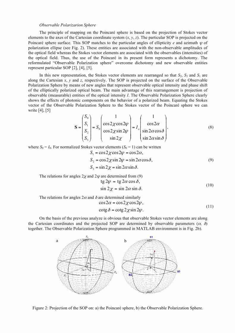
The principle of mapping on the Poincaré sphere is based on the projection of Stokes vector elements to the axes of the Cartesian coordinate system (x, y, z). The particular SOP is projected on the Poincaré sphere surface. This SOP matches to the particular angles of ellipticity e and azimuth ψ of polarization ellipse (see Fig. 2). These entities are associated with the non-observable amplitudes of the optical field whereas the Stokes vector elements are associated with the observables (intensities) of the optical field. Thus, the use of the Poincaré in its present form represents a dichotomy. The reformulated “Observable Polarization sphere” overcome dichotomy and new observable entities represent particular SOP [2], [4], [5].

In this new representation, the Stokes vector elements are rearranged so that S2, S3 and S1 are along the Cartesian x, y and z, respectively. The SOP is projected on the surface of the Observable Polarization Sphere by means of new angles that represent observable optical intensity and phase shift of the elliptically polarized optical beam. The main advantage of this rearrangement is projection of observable (measurable) entities of the optical intensity I. The Observable Polarization Sphere clearly shows the effects of photonic components on the behavior of a polarized beam. Equating the Stokes vector of the Observable Polarization Sphere to the Stokes vector of the Poincaré sphere we can write [4], [5]

⎟⎟⎟⎟⎟

⎠

⎞

⎜⎜⎜⎜⎜

⎝

⎛

=

⎟⎟⎟⎟⎟

⎠

⎞

⎜⎜⎜⎜⎜

⎝

⎛

=

⎟⎟⎟⎟⎟

⎠

⎞

⎜⎜⎜⎜⎜

⎝

⎛

=

δα

δα

α

χ

ψχ

ψχ

sin2sincos2sin2cos1

2sin2sin2cos2cos2cos

1

0

3

2

1

0

oIS

SSSS

S , (8)

where S0 = I0. For normalized Stokes vector elements (S0 = 1) can be written

.sin2sin2sin,cos2sin2sin2cos

,2cos2cos2cos

3

2

1

δαχ

δαψχ

αψχ

==

==

==

SSS

(9)

The relations for angles 2χ and 2ψ are determined from (9)

.sin2sin2sin,cos2tg2tgδαχ

δαψ

=

= (10)

The relations for angles 2α and δ are determined similarly

.2sin2cotgcotg,2cos2cos2cos

ψχδ

ψχα

=

= (11)

On the basis of the previous analyze is obvious that observable Stokes vector elements are along the Cartesian coordinates and the projected SOP are determined by observable parameters (α, δ) together. The Observable Polarization Sphere programmed in MATLAB environment is in Fig. 2b).

Figure 2: Projection of the SOP on: a) the Poincaré sphere, b) the Observable Polarization Sphere.

a)

2α

δ

b)

The relation for angles 2α a δ can be determined from Fig. 2 b) and can be written as

.arctg,tg

,arccos21,2cos

2

3

2

3

0

1

0

1

SS

SS

SS

SS

==

==

δδ

αα

(12)

The relations for the ellipticity and the azimuth of the polarization ellipse can be also derived from the Poincaré sphere in Fig. 2 a) and can be written as

.arcsin21tgtg,arctg

21

0

3

1

2

SS

abe

SSazimut ===== χψ (13)

2 Modelling of photonic components – application The application “Modelling of the photonic components on the Observable Polarization Sphere“

(OPS) is a comprehensive programming environment, shown in Fig. 3. The application enables to study the SOP development of the optical beam which is propagating through the optical system consisting of the fundamental linear photonic components. For modelling of the particular SOP the Muller matrices and the Stokes vector principals are used. The mapping of the SOP on the Observable Polarization Sphere is applied. The application is programmed by means of the Switched board programming method [7], [8]. This method is based on the utilization of Switch, Case instruction commands and the properties of functions to call them-self (callback).

After initiation of the application the panel for entering the required number of matrices (photonic components) is only opened (see Fig. 3). When the required number is inserted and OK button is pressed the second panel is opened. This panel enables to choose the required photonic components by means of ticking the particular radio buttons. For the linear polarizer, linear retarder, rotator are LP, LR, Rot abbreviations used, respectively. To express the right order of the photonic components the ordinal number of matrices is used. For example we can see that M1 is the first component of the optical path and M5 is the last component. The last panel enables to set the required parameters of particular components and insert Stokes vector values of the input optical beam. Whether the projection of the input Stokes vector is required, we can thick radio button Sin.

Figure 3: Modelling of photonic components – application.

When the OK button of the last panel is pressed the processing of the required data is conducted. The particular Mueller matrices with corresponding legend, input and output Stokes vectors and product Mueller matrix are displayed. The projection of the SOP on the Observable Polarization Sphere is also conducted. For better study of the development of the SOP the facilities of rotation and zoom are available by means of vertical and horizontal sliders and zoom on, zoom off buttons. The transmission of data between MATLAB and Microsoft Office Excel is conducted by means of xlswrite and xlsread command instructions, see left bottom in Fig. 3.

To program this application a lot of tasks were needed to sort out. To save and load data the object cell was chosen. This object enables to create cell array of empty matrices. The both type of data text strings and numbers can be applied to the one object unlike matrix. The script for programming of data field of application is shown in Fig. 4. All data are saved to the memory of the particular object with the corresponding handle by means of userdata configuration as shown in the last line in Fig. 4.

Figure 4: Creating of the data field by means of the cell command.

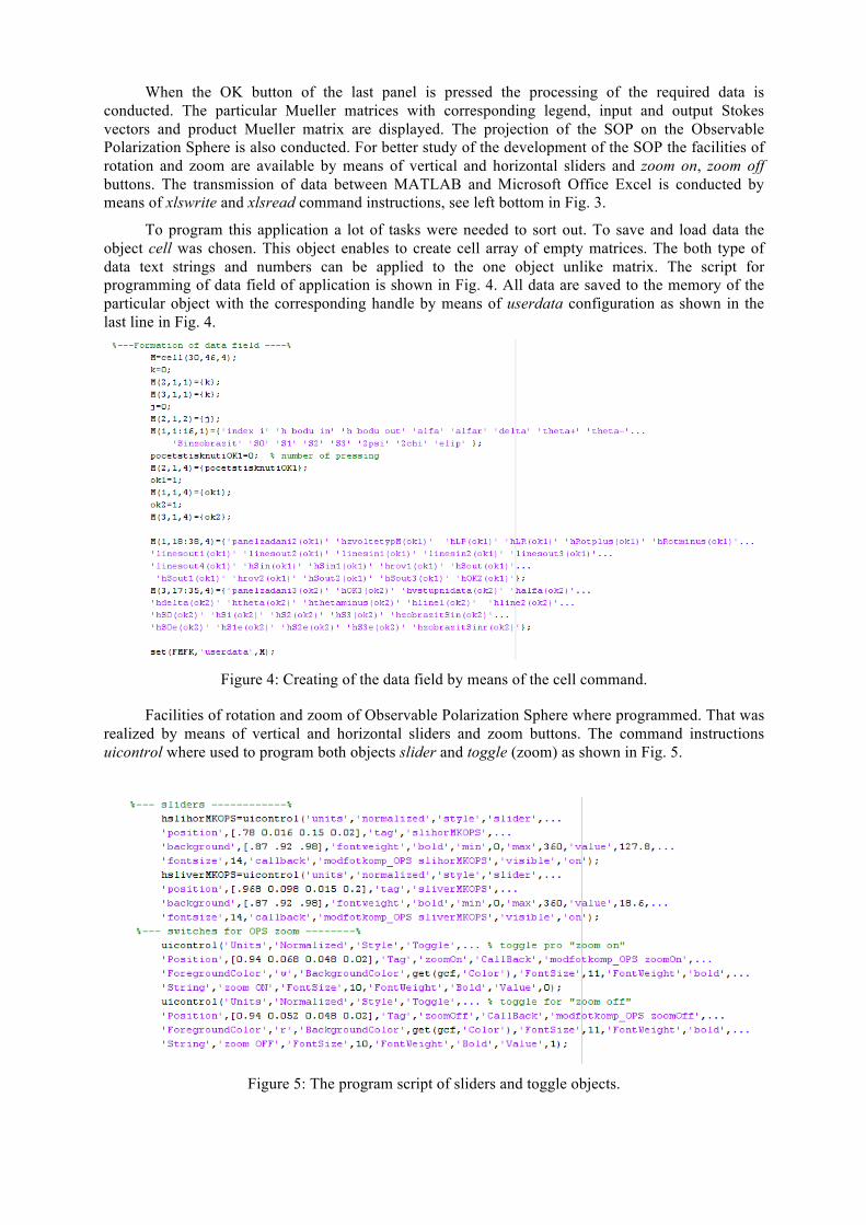
Facilities of rotation and zoom of Observable Polarization Sphere where programmed. That was realized by means of vertical and horizontal sliders and zoom buttons. The command instructions uicontrol where used to program both objects slider and toggle (zoom) as shown in Fig. 5.

Figure 5: The program script of sliders and toggle objects.

The response of sliders and zoom objects is shown in Fig. 6. The rotation of Observable Polarization Sphere is realized by means of get, set and view command instructions. The function zoom is realized by means of the adjustment zoom on or zoom off objects to the value 0 with using the command instructions zoom on and zoom off.

Figure 6: Programming of the response of sliders and zoom buttons.

The example of script for lines that enclose the particular matrix with its legend is in Fig. 5. At first the required number of matrices is fetched from particular object with tag. ‘hpocetmaticMe’. The helping objects and coordinates of matrices are programmed in next step. The projection of required matrices with theirs legend is conducted in cycle by means of command instruction line as shown in Fig. 7.

Figure 7: The program script of matrix projection in application.

3 Comparison with Optisystem 11 Optisystem is a comprehensive software design suite that enables users to plan, test, and

simulate optical links in the transmission layer of modern optical networks. The system enables connection with other systems like MATLAB, SIMULINK, Optispace, Agilent and Scilab. For comparison reason only particular part of Optisystem was applied. The same optical path as shown in Fig. 3 was modeled in Optisystem and is shown in Fig. 8.

Figure 8: The optical path model in Optisystem.

The principle of forming optical path is based on the insertion of icons from the left part of the window to the right active part. It means that left part can be imagined as a library or a source of particular photonic components. By means of clicking upon the particular icon, the window with computed data, parameters and other features is opened. The example of this window for polarization analyzer is shown in Fig. 8. These windows enable insertion of the required values of the particular photonic component parameters. We can see that principle of the creation of the optical path with adjusted components is generally similar. Meanwhile the presented application is more focused to the specific tasks, the Optisystem provide wide range of capabilities. Thus, the different graphical interpretation is obvious. Opposite to the presented application the SOP is projected on the Poincaré sphere and Optisystem doesn’t enable projection on the Observable Polarization Sphere. For conducted analyze the computed results of the output Stokes vector is performed in the table form as shown in Fig. 8. Values of S1, S2 and S3 are presented in normalized form meanwhile S0 is presented in [dBm] unit. This form is more adequate to the projection on the Poincaré sphere, but the relations among the particular Stokes vector elements are less understandable. Presented MATLAB application enables more clearly visualized computed results in Mueller matrices and the Stokes vector form that enables better understanding of the studied phenomenon. The main disadvantage of the Optisystem is an impossibility of projection of SOP development. The Optisystem enables to project only the one SOP at once. In Optisystem we must compute for experimentally obtained Stokes vector elements [9] of measured results to the form of ellipticity and azimuth by (13). The evident mistake of Optisystem

is wrongly computed value of the circular polarization azimuth as shown in Fig.8. Within the frame of testing work with Optisystem the different values (90°, -76°, etc.) of the circular polarization azimuth were obtained. As was mentioned above, for circular polarization the Stokes vector elements S1 and S2 are zero and is confirmed by (13) that we can not compute its azimuth. Thus, the azimuth of circular polarization isn’t mentioned.

Conclusion The chosen MATLAB environment is optimal tool for programming of particular applications

focused to the experimental research work. The method Switched board programming together with particular MATLAB objects and matrix processing of data is efficient instrument to program a number of applications. The presented application is mainly devoted to the experimental work in laboratory and enables get better understanding of studied problems. On the other hand the Optisystem is focused to the engineer style of work, where the exact knowledge of principles and structures of components is not necessary. This conclusion is in accordance with the presentation of producer.

Notes This research work was supported by the research programs of University of Defence PRO 207,

PRO 217 and by the group UDeMAG.

MATLAB® is a registered trade mark of The MathWorksTM, Inc.

References

[1] W. A. Shurcliff. Polarized light, production and use. Cambridge, Massachusetts: Harvard University Press, 1962.

[2] E. Collett. Polarized light in fiber optics. Lincroft, New Jersey (USA), 2003. [3] B. E. A. Saleh, M. C. Teich. Fundamentals of photonics. John Wiley&Sons, USA, second edition

2007. [4] E. Collett, B. Schaefer. Visualization and calculation of polarized light. I. The polarization ellipse,

the Poincaré sphere and the hybrid polarization sphere. Applied optics, vol.47, no. 22, 2008. [5] E. Collett, B. Schaefer. Visualization and calculation of polarized light. II. Applications of the

hybrid polarization sphere. Applied optics, vol.47, no. 22, 2008. [6] A. Howard. Elementary Linear Algebra. John Wiley & Sons, Inc., USA, ninth edition, 2005. [7] K. Zaplatílek, B. Doňar. MATLAB – creating of user applications. BEN-technical literature,

Prague, 2004, (in czech). [8] D. Hanselman, B. Littlefield. Mastering MATLAB® 7. Pearson Prentice Hall®, 2005. [9] M. Born, E. Wolf. Principles of optics. Oxford, England: Pergamon press Ltd., 6th edition 1986.

Filip Dvořák University of Defence, Brno, Czech republic, e-mail: filip.dvorak@unob.cz