modelling of hot water flooding - university of reading · pdf fileuniversity of reading...
TRANSCRIPT

University of Reading
Modelling of Hot Water Flooding
as an
Enhanced Oil Recovery Method
by
Zeinab Zargar
August 2013
Department of Mathematics
Submitted to the Department of Mathematics, University of Reading,
in Partial fulfilment of the requirements for the Degree of Master of Science in
Mathematics of Scientific and Industrial Computation

Acknowledgment
I would like to thank my supervisor Professor Mike Baines for his help and support. I also
would like to acknowledge Alison Morton and Paul Childs for their help and advice. Finally
special thanks to my husband and family for their encouragement and support.

Declaration
I confirm that this is my own work and the use of all materials from other sources has been
properly and fully acknowledged.
Signed ...............................................
Abstract
This dissertation describes and compares two numerical techniques that simulate one dimen-
sional hot water injection. In total four equations are introduced in order to model hot water
injection; the Buckley-Leverett equation, two mass balance equations for water and oil phases
and an energy balance equation, all of which are highly non-linear. The objective of the
mathematical model is to solve these equations under the appropriate initial and boundary
conditions. This solution provides space and time distributions of water and oil pressures,
saturations and temperature. One of the major difficulties with numerical modelling of this
process is the dependence of the fluid properties on the pressure and temperature. In the first
technique, the Buckley-Leverett equation is used to calculate oil and water saturation dis-
tributions which is a nonlinear hyperbolic equation. The second order Lax-Wendroff scheme
is used to solve this equation. The results of the saturations are used in the mass balance
equation, which is a nonlinear equation since its coefficients depend on temperature and pres-
sure. A fully implicit central scheme is used in order to discretize the equation and then the
Newton-Raphson method is used to solve this nonlinear system in order to find the pressure
distribution. Finally, the pressure results are used in the nonlinear energy equation to obtain
the temperature profile. In the second model, the implicit pressure/explicit saturation (IM-
PES) technique is used for the mass balance equations of water and oil phases in order to find
the pressure and saturation distributions, then the results are used in the energy equation to
get temperature profiles. Since all these equations are nonlinear and depend on each other,
the energy equation needs to be coupled with material balance equations. Results show that
saturation front in the first model lag behind that of the second model which can be a result
of incompressibility assumption used in it. The second model has to be applied with some
care as it can be easily become unstable, but if it is used in its stability domain the results
are more reliable.

Contents
1 Introduction 1
2 Characteristics of the Model 4
2.1 Assumptions . . . . . . . . . . . . . . . . . . . . . . . . . . . . . . . . . . . . . 4
2.2 Rock and Fluid Properties Description . . . . . . . . . . . . . . . . . . . . . . 5
2.2.1 Darcy’s Law . . . . . . . . . . . . . . . . . . . . . . . . . . . . . . . . . 5
2.2.2 Porosity . . . . . . . . . . . . . . . . . . . . . . . . . . . . . . . . . . . . 5
2.2.3 Saturation . . . . . . . . . . . . . . . . . . . . . . . . . . . . . . . . . . . 6
2.2.4 Permeabilities . . . . . . . . . . . . . . . . . . . . . . . . . . . . . . . . . 6
2.2.5 Hydrocarbon Viscosity . . . . . . . . . . . . . . . . . . . . . . . . . . . . 7
2.2.6 Phase Mass Density . . . . . . . . . . . . . . . . . . . . . . . . . . . . . 8
2.3 Introducing Model Equations . . . . . . . . . . . . . . . . . . . . . . . . . . . . 9
2.3.1 Buckley-Leverett . . . . . . . . . . . . . . . . . . . . . . . . . . . . . . . 9
2.3.2 Mass Balance Equation . . . . . . . . . . . . . . . . . . . . . . . . . . . 12
2.3.3 Energy Balance Equation . . . . . . . . . . . . . . . . . . . . . . . . . . 13
2.4 Initial and Boundary Conditions . . . . . . . . . . . . . . . . . . . . . . . . . . 14
2.5 Heat losses . . . . . . . . . . . . . . . . . . . . . . . . . . . . . . . . . . . . . . 15
3 First Model 17
3.1 Buckley-Leverett Discretization . . . . . . . . . . . . . . . . . . . . . . . . . . . 17
3.1.1 Effect of boundary conditions . . . . . . . . . . . . . . . . . . . . . . . 19
3.1.2 The CFL condition . . . . . . . . . . . . . . . . . . . . . . . . . . . . . . 20
3.2 Discretization of the Mass balance equation . . . . . . . . . . . . . . . . . . . . 21
3.3 Newton’s Method for Nonlinear Systems of Equations . . . . . . . . . . . . . . 24
3.4 Jacobian Matrix Definition for Mass Balance Equation . . . . . . . . . . . . . . 26
3.5 Well Coupling . . . . . . . . . . . . . . . . . . . . . . . . . . . . . . . . . . . . . 27
3.6 Energy Balance Equation Discretization . . . . . . . . . . . . . . . . . . . . . . 28
3.6.1 Discretization of Right Hand Side of the Energy Equation 3.57 . . . . . 29
3.6.2 Discretization of Left Hand Side of Energy Equation 3.57 for Middle
Cells ( i=2, . . . ,Nx) . . . . . . . . . . . . . . . . . . . . . . . . . . . . . 29
3.6.3 Calculations for the Left Boundary Cell (i=1) . . . . . . . . . . . . . . . 31
3.6.4 Calculations for the Right Boundary Cell (i=Nx) . . . . . . . . . . . . . 32
3.7 Summary of The First Model . . . . . . . . . . . . . . . . . . . . . . . . . . . . 36
4 Second Model 37
4.1 IMPES Technique . . . . . . . . . . . . . . . . . . . . . . . . . . . . . . . . . . 37

4.2 Jacobian Calculations for the Pressure Equation . . . . . . . . . . . . . . . . . 39
4.3 Saturation Calculations . . . . . . . . . . . . . . . . . . . . . . . . . . . . . . . 41
4.4 Summary of the Second Model . . . . . . . . . . . . . . . . . . . . . . . . . . . 42
5 Results 43
5.1 First Model Results . . . . . . . . . . . . . . . . . . . . . . . . . . . . . . . . . 43
5.2 Second Model Results . . . . . . . . . . . . . . . . . . . . . . . . . . . . . . . . 43
5.3 Comparing Two Models . . . . . . . . . . . . . . . . . . . . . . . . . . . . . . . 44
5.4 Sensitivity Analysis . . . . . . . . . . . . . . . . . . . . . . . . . . . . . . . . . . 44
6 Conclusion 54
6.1 Future work . . . . . . . . . . . . . . . . . . . . . . . . . . . . . . . . . . . . . . 54

1 Introduction
A hydrocarbon reservoir is an underground volume comprised of porous rock containing a
mixture of water and hydrocarbon fluids in the form of oil and gas, occupying the void space
of the pores in the rock. Oils can be divided into two categories, light oils and heavy oils.
Light oils have a low viscosity while heavy oils have a high viscosity. The viscosity of a fluid is
a measure of how easily that fluid will flow, for instance, water has a very low viscosity while
honey has a high viscosity.
When oil recovery is high due to high natural reservoir pressure. The rate of natural oil
production will diminish with time, but there are some oil recovery methods to improve the
production rate. Oil recovery processes involve the injection of fluid or a combination of fluid
and chemicals into the oil reservoir via injection wells to force as much oil as possible towards
and, hence, out of the production wells. Light oils are extracted under primary and secondary
recovery methods which involve allowing the fluid to flow out under the natural pressure of its
surrounding. These methods cannot be applied to the extraction of heavy oils, whose viscosity
is far too high for such methods to be effective; their viscosity needs to be reduced. This is
achieved by various thermal stimulation techniques like hot water flooding, steam injection,
in-situ combustion and so far which raise the temperature of the oil, effectively reducing its
viscosity. The approach which is under consideration here is hot water injection modeling. It is
necessary to model and simulate this process in order to provide information about production
and the future of the reservoir to get the best recovery.
All thermal recovery processes tend to raise the temperature of the crude in a reservoir to
reduce the reservoir flow resistance by reducing the viscosity of the crude [12]. It is desirable
to heat the reservoir efficiently, but inevitably some of the heat in the reservoir is lost through
produced fluids, and some is lost to the adjacent overburden and underburden formations.
The heat loss to the adjacent formations is controlled by conduction (heat transfer) which it
can be readily estimated.
In hot water flooding, as can be seen in figure 1.1 many reservoir equivalent volumes of hot
water are injected into a number of wells in order to reduce the viscosity and subsequently
displace the oil in place more easily towards oil production wells. Hot water injection may be
preferred in shallow reservoirs containing oils in the viscosity range of 100-1000 cp [4].
1

Figure 1.1: Schematic diagram of hot water injection process
The mathematical model representing the physical process of hot water injection requires rock
and fluid properties in order to describe the fluid flow and heat transfer with a set of partial
differential equations and algebraic equations, which are derived from physical principals. This
set of equations is derived from four main principles: Conservation of mass of phases (water
and oil); Darcy’s Law for volumetric flow rates which describes how the fluid phases flow
through the reservoir; volume balance equation, a condition which states that the fluid fills
the rock pore volume; conservation of energy of phases. Since the resulting equations are too
complex for more realistic models to be solved using analytic techniques, here is focused on
numerical techniques.
In this dissertation, two different models are applied and analyzed for the hot water injec-
tion process. Chapter 2 contains the problem definition and characteristics of the model.
Introducing some necessary concepts about rock and fluid properties, and required equations.
Initial and boundary conditions and heat loss in our model are also included in this part. The
first model is introduced in chapter 3, where in order to find the saturation distribution the
Buckley-Leverett equation is used. The nonlinear mass balance equation is solved by a fully
implicit central technique by using the results of oil and water saturations from the Buckley-
Levertt equation. Subsequently, the saturation and pressure results are applied to a nonlinear
energy equation discretized by a fully implicit method. Finally, the mass balance equation
2
(pressure equation) and energy balance equation (temperature equation) are coupled to find
the best result for pressure and temperature distribution, since these equations are highly non-
linear. In chapter 4 the second model is presented. In this model, implicit pressure explicit
saturation (IMPES) technique is applied to our hot water model. During one time step, the
results of IMPES are used in the temperature equation which is solved fully implicitly, and
finally there is a coupling between IMPES technique and fully implicit temperature equation
in order to find the final pressure, saturation and temperature distribution results. In both
approaches, bottom hole pressures at the boundaries for the two model are also calculated
using a well coupling method. Because of the complexity of the models we have tried to give
easier understanding of the models by summarizing the models in flowchart diagrams at the
end of each chapter. Chapter 5 shows and compares the results of the two models and some
sensitivity analysis are presented as well. Finally chapter 6 outlines the conclusions which are
drawn from the results.
3

2 Characteristics of the Model
In this project, we have tried to model the hot water flooding process in a reservoir which
is initially saturated with oil and water. The reservoir is considered to be one-dimensional
between an injection and production wells. A schematic diagram of the model is given in
figure 2.1. Hot water is injected with a constant rate and temperature into the porous
media which is filled with cold and heavy oil. In such a system fluid flow, heat transfer
and heat losses are modeled in order to give a better understanding of the process and its
effect on oil recovery.
Figure 2.1: Schematic diagram of the problem
2.1 Assumptions
The following assumptions are made to model the process;
1. In all reservoir processes, every point within the reservoir is in thermodynamics
equilibrium.
2. The injected fluid reaches thermal equilibrium instantaneously with the reservoir
fluids and sand, meaning that all phases and rock in the same location have the same
temperature.
4

3. The model simulates one-dimensional fluid flow and heat convection but two-
dimensional heat conduction throughout the underburden – reservoir –overburden
system.
4. There is a two-phase (water and oil) system which is immiscible.
5. There in no capillary pressure (PO = Pw = P ).
6. Gravity effects are neglected.
2.2 Rock and Fluid Properties Description
The data of rock and fluid properties are required to understand the concept of the model.
Among these, Darcy’s Law, porosity, saturation, permeabilities and phase viscosities and
densities are introduced briefly below.
2.2.1 Darcy’s Law
Darcy’s Law describes the flow of a fluid through a porous medium. It determines how fast
the phases flow through the reservoir and gives the phase velocities [1]. For one dimensional
flow, the Darcy’s phase velocities can be written
Vα = −CαKabs
(∂Pα∂x− ραg
∂d
∂x
)α = Oil, Water (2.1)
where
Cα =Krα
µα(2.2)
denotes phase mobilities (which are phase relative permeabilities divided by phase viscosities)
ρ denotes phase mass densities; ∂d∂x represents the depth gradient; and Kabs is the absolute
permeability of the reservoir; Pα is the pressure of each phase. The fluid flow is therefore due
to a pressure gradient and a gravitational potential, g. In this project, by assumptions 5 and
6 Darcy’ law is simplified to
Vα = −CαKabs
(∂P
∂x
)α = Oil, Water (2.3)
A fuller description of some of the terms in Darcy’ law is now given in more detail.
2.2.2 Porosity
Oil is contained in rocks which are a type of porous media. Porosity is the ratio of void space
over the bulk volume of the rock [1],
5

ϕ =Pore V olume (Vp)
Bulk V olume (Vb)(2.4)
2.2.3 Saturation
The pore volume space is not always filled with a single fluid. Saturation of each fluid (phase)
is defined as the ratio of its volume over the total pore volume occupied by all phases [1],
Si =Phase V olume (Vi)
Pore V olume ( Vp)(2.5)
By definition, the saturations are all non-negative, and sum to one.
2.2.4 Permeabilities
One of the main properties of porous rock is its capability to allow fluid flow through its
connected pores which is known as permeability. There are two definitions of permeability
in the oil industry; absolute and relative permeabilities. Under the condition of single phase
flow, this capability is named absolute permeability. But when the porous media is filled
by more than one phase, due to various ways the phases can occupy the pore volume, the
phases adversely affect the flow of each other in a complicated manner [1]. This effect is
described using phase relative permeabilities, Kro and Krw. The dependence of the relative
permeabilities on the rock and fluid properties is very complicated [2]; the Kro and Krw
considered here are non-negative functions of the saturation, S. In this case, it is necessary
that relative permeabilities must tend to zero as its saturations approaches zero. There are
different methods used to find relative permeabilities. In this project the Corey-type, which
is a power law in the water saturation, Sw, is chosen [3].
Krow (Sw) = Kmax
ro (1− Swn)no no = 3
Krw (Sw) = Kmaxrw .Snwwn nw = 3
(2.6)
where
Swn (Sw) =Sw − Swi
1− Swi − Sorw(2.7)
Krow (Swi) = Kmax
ro , Krow (1− Sor) = 0
Krw (Sw) = 0 , Krw (1− Sor) = Kmaxrw
(2.8)
6

Swi: Irreducible water saturation
Swc: Connate water saturation
Sorw: Residual water saturation (water-oil system )
Sw: Water saturation
Swn: Normalized water saturation
Figure 2.2 shows the results of water and oil relative permeabilities versus water saturation
in the system by applying the Corey correlation.In describing two-phase flow mathematically,
it is always the relative permeability ratio, KroKrw
, versus water saturations (for oil and water
system) that enters the equations.
Figure 2.2: Oil and water relative permeabilities using Corey correlation
2.2.5 Hydrocarbon Viscosity
Phase viscosity represents the resistance of a phase to flow under the influence of a pressure
gradient. The most obvious effect of thermal recovery on a reservoir fluids is the reduction of
oil viscosity. In figure 2.3 two points are evident. First, the rate of viscosity improvement is
greatest as the initial temperature increases. Little viscosity benefit is gained after reaching a
certain temperature. Second, greater viscosity reductions are experienced in the more viscous
low API gravity crudes (API is a degree of measurement for oil density) than in higher API
gravity crudes. Heating from 100oF to 200oF reduces the viscosity, 98% for 10oAPI crudes
but only 73% for 30oAPI oils. These observations show that the greatest viscosity reduction
occurs with the more viscous oils at the initial temperature increases [4].
7

Figure 2.3: Effect of temperature on viscosity
Viscosity is a function of temperature and pressure, but water and oil viscosities are stronger
functions of temperature in a thermal process rather than pressure. Since a thermal oil
recovery method is modeled in this project, the effect of pressure is neglected [5].
µo = 2.626× 10⁸ (T − 459.59)−2.91 (2.9)
µw =2.185
0.04012 (T − 459.59) + 5.154× 10⁻⁶ (T − 459.59)2 − 1(2.10)
2.2.6 Phase Mass Density
Phase density is defined as mass per unit volume for each phase. Water and oil densities
in this context are considered to be a function of temperature and pressure. In the absence
of experimental data, empirical relations are used to express densities of oil and water as
functions of both temperature and pressure [5]:
ρw = 63 exp(17.253× 10⁻⁵ (T − 459.59)
)exp
(4× 10⁻⁶ (P − 1000)
)(2.11)
ρo = 59 exp(−7.5885× 10⁻⁵ (T − 459.59)
)exp
(1× 1−5 (P − 1000)
)(2.12)
Figure 2.4 shows the effect of temperature and pressure increase on the densities of both
phases.
8

Figure 2.4: Effect of temperature and pressure on oil and water densities
2.3 Introducing Model Equations
In the two hot water models presented in this dissertation, four equations are required; the
Buckley-Leverett equation, mass balance equations for water and oil, and an energy Balance
equation.
2.3.1 Buckley-Leverett
The Buckley-Leverett (BL)equation is used in oil recovery in order to find the saturation
distribution in 1D reservoir. In the BL mechanism oil is displaced by water from a rock
in a similar as fluid is displaced from a cylinder by a leaky piston. In order to have better
understanding of the Buckley-Leverett equation, it is first necessary to introduce the fractional
flow equation.
2.3.1.1 Derivation of Fractional Flow for the Model
When oil is displaced by water in the system, from Darcy’s equation we have
qw = −1.127 KabsKrw
µwAx
(∂P
∂x
)(2.13)
9

qo = −1.127 KabsKro
µoAx
(∂P
∂x
)(2.14)
By adding the two equations
qw + qo = −1.127 KabsAx
(Krw
µw+Kro
µo
)∂P
∂x(2.15)
Substituting for
q = qw + qo (2.16)
and
fw =qwq
(2.17)
and solving for the fraction of water flowing, we obtain
fw =1
1 + Kroµo. µwKrw
(2.18)
since
Kr (Sw)⇒ fw(Sw) (2.19)
Now, the Buckley-Leveret equation is derived for a 1D sample based on mass conservation
and some assumptions [6], namely flow is linear and steady state, the fluid is incompressible,
capillary pressure (Pc) is just a function of the saturation and pressure gradient for two phases
is equal (dPcdS = 0), where Pc = Po − Pw.
By applying mass balance of water around a control volume (see figure 2.5) of length 4x we
get the following system for a time period of 4t :
Figure 2.5: Mass Balance Element for Fractional Flow Equation
The material balance may be written:[(ρwqw)x − (ρwqw)x+4x
]4t = A4xϕ
[(ρwSw)t+∆t − (ρwSw)t
](2.20)
which, when ∆x→ 0 and ∆t→ 0 , reduces to the continuity equation:
− ∂
∂x(ρwqw) = Aϕ
∂
∂t(ρwSw) (2.21)
10

by assuming an incompressible fluid ρw = constant and we have that qw = fwq,
Therefore
− ∂fw∂x
=Aϕ
q
∂Sw∂t
(2.22)
Since fw(Sw), equation 2.22 may be rewritten as [6]
− ∂fw∂Sw
∂Sw∂x
=Aϕ
q
∂Sw∂t
(2.23)
where fractional water flow is defined asfs (Scv) = 1
1+KroKw
.µwµo
= 1
1+(Kmaxro )
Kmaxrw
.(
1−SnSn
)3.µwµo
Sn = Sw−Swc1−Swc−Sor Swc < Sw < (1− Sor)
(2.24)
∂fw∂Sw
= 3
(µwµo
) (Kmaxro
Kmaxrw
)(1− Sn)2
(1− Sor − Swc) .S4n.
(1 + Kro
Krw.µwµo .
(1−SnSn
)3)2 (2.25)
fw = f (Kmaxro , Kmax
rw , µo, µw, Swc, Sor, Sw)
Figure 2.6 shows the fractional water flow function and its derivatives as a function of water
saturation
Figure 2.6: Fractional water function and its derivative versus water saturation
Equation 2.22 is known as the Buckley-Leverett equation which is a first order hyperbolic equa-
tion. The equation can be solved analytically by the method of characteristics and graphically
[7]. In this project a second order numerical scheme, the Lax-Wendroff scheme, is used to
solve it. The method is explained in more detail in the following chapters.
11

2.3.2 Mass Balance Equation
The main flow equation in reservoir engineering can simply be derived by applying material
balance to a control volume, as shown in figure 2.7. Mass accumulation inside a control volume
is the difference between input and generated mass and output and consumed mass as below:
˙(mi − mo)− (mcons − mgen) =∂M
∂t, m = Mass F lux = ρ . q (2.26)
whereq is flow rate , ρ is density , M is mass and t is time. Time
Based on what we have in equation 2.26 for 1D flow, the input mass rate for x direction shown
in figure 2.7 will be:
mix = ρ . ux .dAx (2.27)
dAx, ux and ρ are the normal cross sectional area in x direction, velocity and density respec-
tively.
Figure 2.7: Material Balance Control Volume
Using the Euler approximation for the mass rate
mi(x+dx) = mo = mi(x) +∂mix
∂x. dx (2.28)
The generation and consumption terms in reservoir engineering are production and injection
in wells and can be specified as:
mcons = ρ . qprod , qprod = Production Rate
mgen = ρ . qinj , qinj = Injection Rate(2.29)
By substituting equations 2.27 , 2.28 and 2.29 in equation 2.26:
− ∂
∂x(ρ.ux.dy.dz) .dx− (ρ.qp − ρ.qi) =
∂
∂t(ρ.ϕ. dx.dy.dz) (2.30)
Using Vb = dx . dy. dz and dividing both sides to Vb gives:
− ∂
∂x(ρ.ux)− 1
Vb(ρ.qprod − ρ.qinj) =
∂
∂t(ρ.ϕ) (2.31)
12

Equation 2.31 is the most general type of the mass conservation law in its one dimensional
form [8]. To make it more usable in reservoir engineering, Darcy law (equation 2.3) is used to
substitute the velocities. Hence, the result for multi-phase flow in porous media will be
∂
∂x
(ραµαKabsKrα
∂P
∂x
)− ραVb
(qprod − qinj) =∂
∂t(ρα.Sα.ϕ) (2.32)
In this dissertation, α denotes water and oil phases.
2.3.3 Energy Balance Equation
Thermal simulation is all about energy balance and temperature calculations. The energy
conservation law is very similar to the mass conservation law and can be written as:
(ei − eo)− (econs − egen) =∂E
∂t, e = Energy F lux (2.33)
In hot water modeling, the energy consumption and generation are related to injection or
production streams. There are two main heat transfer equations that are widely used for
energy balance, conduction and convection which are defined as,
Conduction heat transfer; q = −k. ∂T∂xConvection heat transfer; q = ρ.−→u .H
where k is thermal conductivity and H is enthalpy.
Therefore, the energy at each point can be written as:
e =
(−k.∂T
∂x+ ρ.−→u .H
)× Cross section area (2.34)
Similar to mass balance, energy balance can also be driven by applying equation 2.33 and
equation 2.34 on a single element like the one shown in figure 2.8.
Figure 2.8: Energy balance element
ex = eix =
(−k.∂T
∂x+ ρ.ux.H
)dydz (2.35)
13
e(x+dx) = eox =
[(−k.∂T
∂x+ ρ.ux.H
)+
∂
∂x
(−k.∂T
∂x+ ρ.ux.H
).dx
]dydz (2.36)
eix − eox =
(k∂2T
∂x2− ∂
∂x(ρ.ux.H)
)dxdydz =
(k∂2T
∂x2
)dxdydz +
∂
∂x
(ρ
µ.K.H.
∂P
∂x
)dxdydz
(2.37)
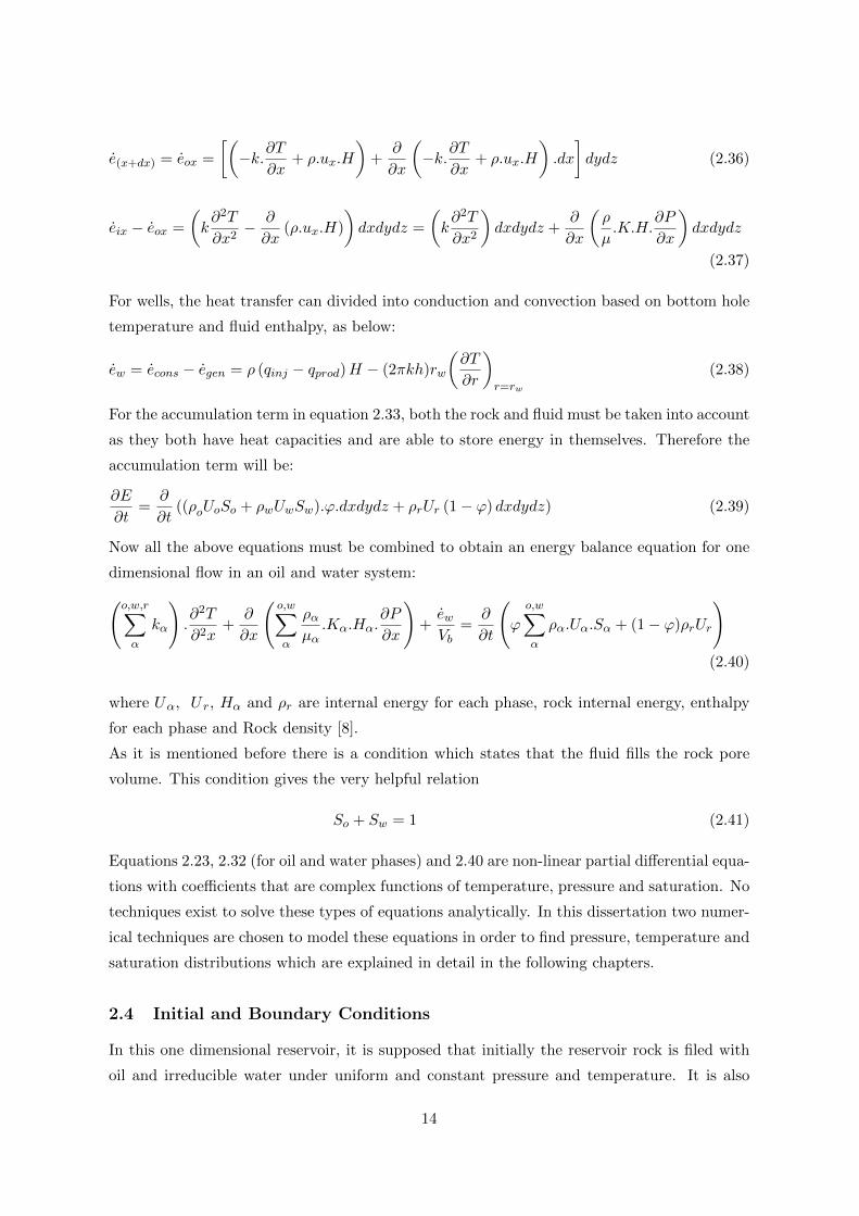
For wells, the heat transfer can divided into conduction and convection based on bottom hole
temperature and fluid enthalpy, as below:
ew = econs − egen = ρ (qinj − qprod)H − (2πkh)rw
(∂T
∂r
)r=rw
(2.38)
For the accumulation term in equation 2.33, both the rock and fluid must be taken into account
as they both have heat capacities and are able to store energy in themselves. Therefore the
accumulation term will be:
∂E
∂t=
∂
∂t((ρoUoSo + ρwUwSw).ϕ.dxdydz + ρrUr (1− ϕ) dxdydz) (2.39)
Now all the above equations must be combined to obtain an energy balance equation for one
dimensional flow in an oil and water system:(o,w,r∑α
kα
).∂2T
∂2x+
∂
∂x
(o,w∑α
ραµα.Kα.Hα.
∂P
∂x
)+ewVb
=∂
∂t
(ϕ
o,w∑α
ρα.Uα.Sα + (1− ϕ)ρrUr
)(2.40)
where Uα, U r, Hα and ρr are internal energy for each phase, rock internal energy, enthalpy
for each phase and Rock density [8].
As it is mentioned before there is a condition which states that the fluid fills the rock pore
volume. This condition gives the very helpful relation
So + Sw = 1 (2.41)
Equations 2.23, 2.32 (for oil and water phases) and 2.40 are non-linear partial differential equa-
tions with coefficients that are complex functions of temperature, pressure and saturation. No
techniques exist to solve these types of equations analytically. In this dissertation two numer-
ical techniques are chosen to model these equations in order to find pressure, temperature and
saturation distributions which are explained in detail in the following chapters.
2.4 Initial and Boundary Conditions
In this one dimensional reservoir, it is supposed that initially the reservoir rock is filed with
oil and irreducible water under uniform and constant pressure and temperature. It is also
14
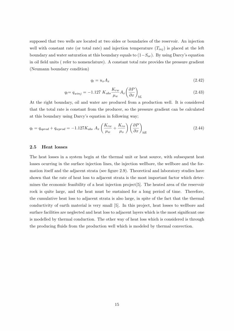
supposed that two wells are located at two sides or boundaries of the reservoir. An injection
well with constant rate (or total rate) and injection temperature (Tinj) is placed at the left
boundary and water saturation at this boundary equals to (1−Sor). By using Darcy’s equation
in oil field units ( refer to nomenclature). A constant total rate provides the pressure gradient
(Neumann boundary condition)
qt = uxAx (2.42)
qt= qwinj = −1.127 KabsKrw
µwAx
(∂P
∂x
)bL
(2.43)
At the right boundary, oil and water are produced from a production well. It is considered
that the total rate is constant from the producer, so the pressure gradient can be calculated
at this boundary using Darcy’s equation in following way;
qt = qoprod + qwprod = −1.127Kabs Ax
(Krw
µw+Kro
µo
)(∂P
∂x
)bR
(2.44)
2.5 Heat losses
The heat losses in a system begin at the thermal unit or heat source, with subsequent heat
losses ocurring in the surface injection lines, the injection wellbore, the wellbore and the for-
mation itself and the adjacent strata (see figure 2.9). Theoretical and laboratory studies have
shown that the rate of heat loss to adjacent strata is the most important factor which deter-
mines the economic feasibility of a heat injection project[5]. The heated area of the reservoir
rock is quite large, and the heat must be sustained for a long period of time. Therefore,
the cumulative heat loss to adjacent strata is also large, in spite of the fact that the thermal
conductivity of earth material is very small [5]. In this project, heat losses to wellbore and
surface facilities are neglected and heat loss to adjacent layers which is the most significant one
is modelled by thermal conduction. The other way of heat loss which is considered is through
the producing fluids from the production well which is modeled by thermal convection.
15

Figure 2.9: Illustration of heat losses which occur in a heat injection system
16

3 First Model
In this model, the Buckley-Leverett equation is used to find saturation profiles and then its
results are used in the pressure equation which is solved by a fully implicit numerical technique.
In order to find the temperature profile the saturation and pressure results are applied to a
fully implicit energy equation. Finally, the mass balance equation (pressure equation) and
the energy balance equation (temperature equation) are coupled to find the optimal result for
pressure and temperature distributions, since these equations are highly nonlinear.
3.1 Buckley-Leverett Discretization
In this model, the Buckley- Leverett equation is used to find the saturation distribution. The
numerical scheme used to solve this hyperbolic equation is the Lax-Wendroff scheme. The
scheme is a second order finite difference method where the derivatives are approximated by
differences of discrete values. An important requirement of numerical methods for such non-
linear hyperbolic equations is to be in conservative form to maintain the conservation property
of the equation. To derive the numerical method in conservative form we use standard finite
difference discretization of the conservative form of the partial differential saturation equation,
not the quasilinear form of the equation.
For a numerical scheme to be in conservation form [9] it must have the form
Un+1j = Unj −
4t4X{F (U
n+ 12
j+ 12
)− F (Un+ 1
2
j− 12
)}, (3.1)
where Unj is an approximation to the cell average of the analytic function, F(U
n+ 12
j+ 12
) is the
numerical flux function, 4t =tn+1−tn, and 4x =xj+ 12−xj− 1
2.
By using oil field units ( refer to nomenclature), the Buckley-Leverett equation will be,
(Aϕ
5.615 qt
)∂S
∂t+∂f
∂x= 0 (3.2)
By choosing,
17
X = xL ⇒ dX = 1
Ldx⇒∂...∂x = 1
L∂...∂X
tD = 5.615 qtA.ϕ.L t⇒ dtD = 5.615
A.ϕ.L dt
⇒ ∂...∂t = 5.615qt
A.ϕ.L∂...∂tD
(3.3)
the BL equation converts into the dimensionless equation,
∂S
∂tD+∂f
∂X= 0 (3.4)
In order to drive the Lax-Wendroff scheme applied to above equation to be in conservative
form, for all intermediate blocks (i = 2, . . . , Nx − 1), we start with;
∂S
∂tD+∂f
∂X= 0 ⇒ ∂S
∂tD= − ∂f
∂X(3.5)
and using Taylor-series expansion about tD
S (Xi, tD + ∆tD) = S (Xi, tD) + ∆tD∂S (Xi, tD)
∂tD+
∆t2D2
∂2S (Xi, tD)
∂t2D+O (∆tD)3 (3.6)
∂S∂tD
= − ∂f∂X
∂2S∂t2D
= − (fs)tD = − (ftD)X = −(∂f∂S .
∂S∂tD
)X
= −(∂f∂S (−fX)
)X
=(∂f∂S .
∂f∂X
)X
(3.7)
By substituting central differences for space derivatives
Sn+1i = Sni −∆tD
(fi+1−fi−1
2∆X
)+
∆t2D2
[( ∂f∂S .
∂f∂X )
i+ 12−( ∂f∂S .
∂S∂X )
i− 12
∆X
]Sn+1i = Sni −
∆tD∆x
[hi+ 1
2− hi− 1
2
]: Conservative form
(3.8)
⇒ By comparison:
hi+ 12
=1
2(fi+1 + fi)−
∆tD2
(∂f
∂S.∂f
∂X
)i+ 1
2
=1
2(fi+1 + fi)−
1
2νi+ 1
2. (fi+1 − fi) (3.9)
where
νi+ 12
=
∆tD∆X
(fi+1−fiSi+1−Si
)if Si 6= Si+1
∆tD∆X
(∂f∂S
)i
if Si = Si+1
(3.10)
18

Similarly hi− 12
= 12 (fi + fi−1)− νi− 1
2(fi − fi−1)
νi− 12
=
∆tD∆X
(fi−fi−1
Si−Si−1
)if Si 6= Si−1
∆tD∆X
(∂f∂S
)i−1
if Si = Si−1
(3.11)
3.1.1 Effect of boundary conditions
For the first cell (i = 1), it is supposed that there is a known value of S at the boundary
(S = 1−Sor). At this point the Lax-Wendroff scheme is derived based on the unequal spacing
(see figure 3.1)
Figure 3.1: Unequal spacing for the left boundary cell after introducing an imaginary node
f (X1 + ∆X) = f (X1) + ∆X.(∂f∂X
)X1
f (X1 −∆Xb) = f (X1)−∆Xb.(∂f∂X
)X1
⇒(∂f
∂X
)X1
=f2 − fb
∆X + ∆Xb(3.12)
Sn+11 = Sn1 −∆tD
(f2 − fb
∆X + ∆Xb
)+
(∆t2D
2
)(∂f∂S .
∂f∂X
)1+ ∆X
2
−(∂f∂S .
∂f∂X
)1−∆Xb
2
∆X/2 + ∆Xb/2
(3.13)
= Sn1 −∆tD
(∆X + ∆Xb)
{(f2 − fb)−∆tD
[(∂f
∂S.∂f
∂X
)1+ ∆X
2
−(∂f
∂S.∂f
∂X
)1−∆Xb
2
](3.14)
⇒
Sn+11 = Sn1 −
∆tD(∆X+∆Xb)
.(h1+ ∆X
2− h
1−∆Xb2
)h1+ ∆X
2= (f2 + f1)− ν1+ ∆X
2. (f2 − f1)
h1−∆Xb
2
= (f1 + fb)− ν1−∆Xb2
(f1 − fb)
(3.15)
19
where
ν1+ ∆X2
=
∆tD∆X .
f2−f1
S2−S1S2 6= S1
∆tD∆X .
(∂f∂S
)1
S2 = S1
ν1−∆Xb
2
=
∆tD∆Xb
. f1−fbS1−Sb Sb 6= S1
∆tD∆Xb
.(∂f∂S
)b
Sb = S1
(3.16)
All the fractional water values and its derivatives in above formulas are calculated from equa-
tions 2.24 and 2.25
For last cell (i =Nx), the equation 3.4 is discretized based on forward in time and backward
in space as follows,
Sn+1i − Sni
∆tD+f (Sni )− f
(Sni−1
)∆X
= 0 (3.17)
⇒ Sn+1i = Sni −
(∆tD∆X
) [f (Sni )− f
(Sni−1
)](3.18)
Finally, the result for all grid points is a linear system, which we denote it by
A.S = b (3.19)
where A is a tridiagonal matrix and S is a vector of unknowns (saturations), which is solved
to find the saturation profile.
3.1.2 The CFL condition
In order to have stability when using explicit numerical schemes, we are required to apply the
necessary condition known as the Courant-Friedrichs-Lewy condition. It is often referred to
as the CFL or Courant condition, [9] and [10], and is
µ=
∣∣∣∣a4t
4x
∣∣∣∣ ≤ µmax (3.20)
Where in this context, a = a (S) = ∂f∂S . Here 4t and 4x are the time and space steps, respec-
tively. The value of µmax changes with the method used to solve the discretized equation.
This condition is not sufficient for stability, as it is only a necessary condition for scheme to
be stable. The Lax-Wendroff scheme is known to be stable for the region µ=∣∣∣a4t4x
∣∣∣ ≤ 1.
The picture on the right of figure 3.2 shows the domain of dependence for this numerical
scheme. If a4t4x is the slope of AB then the CFL condition is satisfied because AB lies in
20

the stencil of the scheme, whilst the line AC violates the CFL condition, by lying outside the
domain of dependence.
Figure 3.2: Stencils for the Lax-Wendroff scheme
3.2 Discretization of the Mass balance equation
The equation 2.32 in oil field units ( refer to nomenclature), for oil phase and substituting
So = 1− S results in
∂
∂x
(ρoµoKabsKro
∂p
∂x
)− ρo
1.127Vb(qp − qi) =
1
6.328
∂
∂t(ρo.(1− S).ϕ) (3.21)
In order to discretize this equation, a fully implicit scheme is used. As mentioned before, the
coefficients of this equation depend on pressure, temperature and saturation. The results of
the saturation from the Buckley-leverett equation are used directly and indirectly (through
the relative permeability) in this equation.
In order to expand the right hand side of equation 3.21, we need to remember that density is
a function of pressure and temperature ( ρ = ρ(p (t) , T (t))), so we have
∂ρo∂t
=∂ρo∂p
.∂p
∂t+∂ρo∂T
.∂T
∂t= ρ′op.
(∂p
∂t
)+ ρ′oT
(∂T
∂t
)(3.22)
Hence, expansion of the equation 3.21 results in
∂
∂x
(ρoKo
µo
∂ρ
∂x
)+
ρoΣqo1.127Vb
=ϕ
6.328
[(1− S) ρ′op.
∂p
∂t+ (1− S) ρ′oT
∂T
∂t− ρ0
∂S
∂t
](3.23)
21
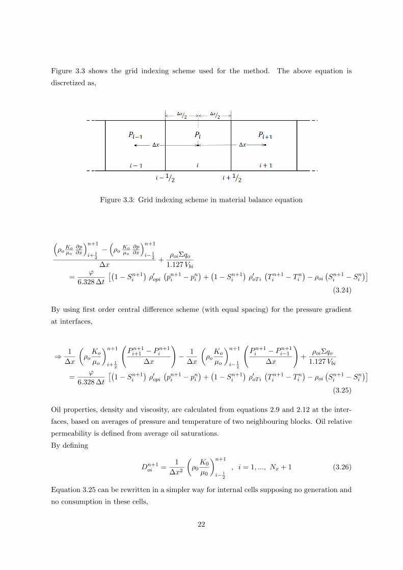
Figure 3.3 shows the grid indexing scheme used for the method. The above equation is
discretized as,
Figure 3.3: Grid indexing scheme in material balance equation
(ρo
Koµo
∂p∂x
)n+1
i+ 12
−(ρo
Koµo
∂p∂x
)n+1
i− 12
∆x+
ρoiΣqo1.127Vbi
=ϕ
6.328 ∆t
[(1− Sn+1
i
)ρ′opi
(pn+1i − pni
)+(1− Sn+1
i
)ρ′oT i
(Tn+1i − Tni
)− ρoi
(Sn+1i − Sni
)](3.24)
By using first order central difference scheme (with equal spacing) for the pressure gradient
at interfaces,
⇒ 1
∆x
(ρoKo
µo
)n+1
i+ 12
(Pn+1i+1 − P
n+1i
∆x
)− 1
∆x
(ρoKo
µo
)n+1
i− 12
(Pn+1i − Pn+1
i−1
∆x
)+
ρoiΣqo1.127Vbi
=ϕ
6.328 ∆t
[(1− Sn+1
i
)ρ′opi
(pn+1i − pni
)+(1− Sn+1
i
)ρ′oT i
(Tn+1i − Tni
)− ρoi
(Sn+1i − Sni
)](3.25)
Oil properties, density and viscosity, are calculated from equations 2.9 and 2.12 at the inter-
faces, based on averages of pressure and temperature of two neighbouring blocks. Oil relative
permeability is defined from average oil saturations.
By defining
Dn+1oi =
1
∆x2
(ρ0K0
µ0
)n+1
i− 12
, i = 1, ..., Nx + 1 (3.26)
Equation 3.25 can be rewritten in a simpler way for internal cells supposing no generation and
no consumption in these cells,
22

Dn+1oi+1
(pn+1i+1 − p
n+1i
)−Dn+1
oi
(pn+1i − pn+1
i−1
)=
ϕ
6.328 ∆t
[(1− Sn+1
i
)ρ′opi
(pn+1i − pni
)+(1− Sn+1
i
)ρ′oT i
(Tn+1i − Tni
)− ρoi
(Sn+1i − Sni
)](3.27)
So, general oil pressure equation for each middle cell (i=2,. . . ,Nx−1) is defined as a function
of three variable pi+1, pi and pi−1,
Dn+1oi .pn+1
i−1 −(Dn+1oi +Dn+1
oi+1 +ϕ
6.328 ∆t
(1− Sn+1
i
)ρ′opi
)pn+1i +Dn+1
oi+1pn+1i+1 =
− ϕ
6.328 ∆t
(1− Sn+1
i
)ρ′opi. p
ni +
ϕ
6.328 ∆t
(1− Sn+1
i
)ρ′oT i
(Tn+1i
− Tni −ϕ
6.328 ∆tρoi(Sn+1i − Sni
) (3.28)
Treating the equation for boundary cells is slightly different. For the first cell (i = 1), the
equation 3.23 is discretized as
(ρo
Koµo
∂P∂x
)n+1
i+ 12
−(ρo
Koµo
∂P∂x
)n+1
bl
∆x+
ρoiΣqo1.127Vbi
=ϕ
6.328 ∆t
[(1− Sn+1
i
)ρ′opi
(pn+1i − pni
)+(1− Sn+1
i
)ρ′oT i
(Tn+1i − Tni
)− ρoi
(Sn+1i − Sni
)](3.29)
Using equation 2.43 and boundary conditions help to find water properties and boundary
pressure gradient in above equation,
Sb = 1− Sor , Tb = Tinj , pb = pbl
Kwbl = Kabs.Krw (1− Sor) = Kabs.Kmaxrw
µwb = µw (Pbl, Tinj)
Pi − Pbl(∆x/2
) =
(∂P
∂x
)bl
= − qt.µwbl1.127KwblAn
= −GPI
(3.30)
Note that the injection well is located on the boundary, so the effect of generation terms is
considered in the boundary pressure gradient. Hence, the discretized oil pressure equation for
the first cell (i = 1) is
−
(Dn+1oi+1 +
ϕ(1− Sn+1
i
)ρ′opi
6.328 ∆t
)pn+1i +Dn+1
oi+1. pn+1i+1 = −Dn+1
oi .∆x.GPI
−ϕ(1− Sn+1
i
)ρ′opi
6.328 ∆tPni +
ϕ (1− Si) ρ′oT i6.328 ∆t
(Tn+1i − Tni
)− ϕρoi
6.328 ∆t
(Sn+1i − Sni
) (3.31)
23

Condition at the right boundary cell is different. Using equation 2.44 and defining a new
parameter, λtb, the pressure gradient for this boundary is calculated as
λtb =Krob
µob+Krwb
µwb⇒
(∂P
∂x
)b
= − qt1.127KabsAn λtb
= −GPO (3.32)
Boundary
conditions
(i = Nx)
Sb = 3
2 SNx −12 SNx−1
pb = pbr
Tb = 32 TNx −
12TNx−1x−1
⇒
Krob = Kro (1− Sb)Krwb = Krw (Sb)
µob = µo (pb, Tb)
µwb = µw (pb, Tb)
By substituting this term into the equation below (discretized pressure equation for the last
cell),
(ρo
Koµo
∂P∂x
)n+1
br−(ρo
Koµo
∂P∂x
)n+1
i− 12
∆x
=ϕ
6.328 ∆t
[(1− Sn+1
i
)ρ′opi
(pn+1i − pni
)+(1− Sn+1
i
)ρ′oT i
(Tn+1i − Tni
)− ρoi
(Sn+1i − Sni
)](3.33)
And noting that the generation and consumption term in the main equation 3.21 is replaced by the
effect of the boundary condition, we have the equation below for = Nx ,
Dn+1oi Pn+1
i−1 −
(Dn+1oi +
ϕ(1− Sn+1
i
)ρ′opi
6.328 ∆t
)Pn+1i = −Dn+1
oi .∆x.GPO
−ϕ(1− Sn+1
i
)ρ′opi
6.328 ∆tPni +
ϕ(1− Sn+1
i
)ρ′oT i
6.328 ∆t
(Tn+1i − Tni
)− ϕρoi
6.328∆t
(Sn+1i − Sni
) (3.34)
Finally, writing these equations for all grid blocks, we obtain the nonlinear system of AS = b
( where A is a tridiagonal matrix in which all its elements depend on the unknowns).Such a
system is not easy to solve, but in the following section we explained how to deal with this
difficulty.
3.3 Newton’s Method for Nonlinear Systems of Equations
To find the solution of a system (Ax = b) of Nx nonlinear equations in Nx unknowns [13], the
system can be written in the homogenous form
24

F (x) = Ax−B = 0 (3.35)
Consider the Taylor-Series expansion of F (x) about x = x0. Using only the first two terms of
the expansion, a first approximation to the root of F (x) can be obtained from
F (x) = F (x0 + ∆x) = F (x0) + (x− x0)∂F
∂x
∣∣∣∣∣ x0
Let ∂F∂x
∣∣∣∣∣ x0
= J (x0) giving F (x) = F (x0) + J (x0) (x− x0) = 0
⇒ (Ax0 −B) + J (x0) . (x− x0) = 0
⇒ (Ax0 −B) + J (x0) . x− J (x0) . x0 = 0
⇒ J (x0) . x = J (x0) .x0 − (Ax0 −B)
If AC = J (x0) , C = J (x0) . x0 − (Ax0 −B)
and x = x0 (a vector) represents the first guess of the solution, successive approximation to
the solution are obtained from
AC .x = C (3.36)
This is the Newton (Newton-Raphson) method for solving the system. It requires the evalu-
ation of the Jacobian matrix of the system which is defined as:
∂F
∂x
∣∣∣∣∣ x = J (x) =
∂F1∂x1
∂F1∂x2
· · · · · · ∂F1∂xN
∂F2∂x1
∂F2∂x2
· · · · · · ∂F2∂xN
......
......
∂FN∂x1
∂FN∂x2
· · · · · · ∂FN∂xN
(3.37)
Different convergence criteria can be applied to the system, to find the solution. In this
project, the maximum of the modulus difference of the between consecutive vectors is used to
be less than a certain tolerance (ε). In mathematical terms this is expressed as
max∣∣xn+1 − xn
∣∣ < ε (3.38)
The main complication with using Newton-Raphson to solve such a system of non-linear
equations is having to define all the functions ∂Fi∂xj
, for i, j = 1, 2, . . . , Nx, included in the
25

Jacobian. As the number of equations and unknowns, Nx , increases, so do the number of
elements in the Jacobian.
The convergence of Newton’s method is quadratic when the Jacobian matrix is non-singular
and the initial guess is close enough.
3.4 Jacobian Matrix Definition for Mass Balance Equation
In order to solve the nonlinear system resulted from applying fully implicit method to oil mass
conservation equation (oil pressure equation), the Jacobian is defined as follow,
For internal equations (i = 2, . . . , Nx − 1)
Fi(Pi−1, Pi, Pi+1) = Dn+1oi .pn+1
i−1 −(Dn+1oi +Dn+1
oi+1 +ϕ
6.328 ∆t
(1− Sn+1
i
)ρ′opi
)pn+1i +Dn+1
oi+1pn+1i+1
+ϕ
6.328 ∆t
(1− Sn+1
i
)ρ′opi. p
ni −
ϕ
6.328 ∆t
(1− Sn+1
i
)ρ′oT i
(Tn+1i − Tni
)+
ϕ
6.328 ∆tρoi(Sn+1i − Sni
)= 0
(3.39)
∂Fi∂Pi
=1
2Dn+1oi ηn+1
opi Pn+1i−1 −
(Dn+1oi +Dn+1
oi+1 +ϕ
6.328 ∆t
(1− Sn+1
i
)ρ′opi
)η(
Dn+1oi
2ηn+1opi +
Dn+1oi+1
2ηn+1opi+1 +
ϕ
6.328 ∆t
(1− Sn+1
i
)ρ′′oppi
)Pn+1i
+1
2Dn+1oi+1 η
n+1opi+1 P
n+1i+1 +
ϕ
6.328∆t
(1− Sn+1
i
)ρ′′oppi P
ni
− ϕ
6.328 ∆t
(1− Sn+1
i
)ρ′′oPT i
(Tn+1i − Tni
)+
ϕ
6.328 ∆tρ′opi
(Sn+1i − Sni
)(3.40)
∂Fi∂Pi−1
= Dn+1oi +
1
2Dn+1oi ηn+1
opi Pn+1i−1 −
1
2Dn+1oi ηn+1
opi Pn+1i = Dn+1
oi
[1 +
1
2ηn+1oi
(Pn+1i−1 − P
n+1i
)](3.41)
∂Fi∂Pi+1
= Dn+1oi+1
[1 +
1
2ηn+1opi+1
(Pn+1i+1 − P
n+1i
)](3.42)
For the first equation (i = 1)
∂Fi∂Pi
= −
(Dn+1oi+1 +
ϕ(1− Sn+1
i
)ρ′opi
6.328 ∆t
)−
(1
2ηn+1opi+1D
n+1oi+1 +
ϕ(1− Sn+1
i
)ρ′′oppi
6.328 ∆t
)Pn+1i
+1
2ηn+1opi+1D
n+1oi+1 P
n+1i+1 +
3
2GPI.∆x ηn+1
opi Dn+1oi +
3
2GPI.∆x.Dn+1
oi .µ′wpbµwb
+ϕ(1− Sn+1
i
)ρ′′oppi
6.328 ∆tPni −
ϕ(1− Sn+1
i
)ρ′′opT i
6.328 ∆t
(Tn+1i − Tni
)+
ϕρ′opi6.328 ∆t
(Sn+1i − Sni
)26

(3.43)
∂Fi∂Pi+1
=1
2ηn+1opi+1D
n+1oi+1
(Pn+1i+1 − P
n+1i
)+Dn+1
oi+1
− 1
2GPI.∆x. ηn+1
opi Dn+1oi − 1
2GPI.∆x.Dn+1
oi .µ′wpbµwb
(3.44)
For the last equation (i = Nx)
∂Fi∂Pi
=1
2Dn+1oi ηn+1
opi Pn+1i−1 −
(Dn+1oi +
ϕ(1− Sn+1
i
)ρ′opi
6.328∆t
)
−
(1
2Dn+1oi ηn+1
opi +ϕ(1− Sn+1
i
)ρ′′oppi
6.328∆t
)Pn+1i − 3
2Dn+1oi ηn+1
opi ∆x.GPO
+ϕ(1− Sn+1
i
)ρ′′oppi
6.328∆tPni −
ϕ(1− Sn+1
i
)ρ′′opT i
6.328∆t
(Tn+1i − Tni
)+
ϕρ′opi6.328∆t
(Sn+1i − Sni
)(3.45)
∂Fi∂Pi−1
= Dn+1oi
(1 +
1
2ηopi
(Pn+1i−1 − P
n+1i
))+
1
2Dn+1oi ηn+1
opi ∆x.GPO (3.46)
where
ηn+1opi =
(ρ′opρo−µ′opµo
)n+1
i− 12
i = 1, ..., Nx + 1 (3.47)
Derivatives of oil and water densities and viscosities to pressure and temperature are defined
using the equations 2.9 - 2.12.
3.5 Well Coupling
In order to find bottom hole pressures at the left and right boundaries, coupling between
the block and well pressures is performed. It starts by taking initial guesses for boundary
(well) pressures. Grid pressures are then solved based on these guesses. Because block and
well pressures are correlated, new well pressures can be calculated from equations 3.48 and
3.49 and these new values used in a new iteration to calculate new grid pressures. Iterations
continue to find fixed block and well pressures. These two equations are nonlinear for the well
pressures, the Newton-Raphson method is used to find the roots.
The left boundary well pressure equation is
qt= −1.127KabsK
maxrw An
µw(Pwl)
PB − Pwl∆x/2
(3.48)
27

The right boundary well pressure equation is
qt=1.127KabsAn
∆x/2
{Krw
µw(Pwr)+
Kro
µo(Pwr)
}(Pwr − PB) (3.49)
3.6 Energy Balance Equation Discretization
The energy equation 2.40 in oil field units ( refer to nomenclature) is rewritten as
∂
∂x.(24KH
∂T
∂x) + 6.328
∂
∂x.{(ρo
Ko
µoHo + ρw
Kw
µwHw)
∂P
∂x}+
Σe
V b
=∂
∂t{ϕ(ρoSoUo + ρwSwUw) + (1− ϕ)ρrUr}
(3.50)
Hα = Hrefα + CPα(T − Tref ) α = o, w
Uα = U refα + CV α(T − Tref ) α = o, w, r(3.51)
A fully implicit central finite difference scheme is used to discretize the equation. First, the
equation is expanded by substituting equation 3.51 and then new equation is shortened by
defining some parameters,
∂
∂x.(24KH
∂T
∂x) + 6.328
∂
∂x.{(ρo
Ko
µo(Href
o + CPo(T − Tref ))∂P
∂x}
+ 6.328∂
∂x{ρw
Kw
µw(Href
w + CPw(T − Tref ))∂P
∂x}+
Σe
V b=
∂
∂t{ϕ(ρoSo(U
refo + CV o(T − Tref )) + ρwSw(U refw + CV w(T − Tref )))
+ (1− ϕ)ρr(Urefr + CV r(T − Tref ))}
(3.52)
By defining,
HR = ρoKo
µo(Href
o − CPoTref ) + ρwKw
µw(Href
w − CPwTref ) (3.53)
HB = ρoKo
µoCPo + ρw
Kw
µwCPw (3.54)
UR = ϕ (ρoSo(Urefo −CV oTref ) + ρwSw(U refw −CV wTref )) + (1−ϕ)ρr(U
refr −CV rTref ) (3.55)
UB = ϕ (ρoSoCV o + ρwSwCV w) + (1− ϕ)ρrCV r (3.56)
Equation 3.52 is simplified to
28

∂
∂x.(24KH
∂T
∂x) + 6.328
∂
∂x((HR+HB.T )
∂P
∂x) +
∑e
Vb=
∂
∂t(UR+ UB × T ) (3.57)
3.6.1 Discretization of Right Hand Side of the Energy Equation 3.57
Replace the derivatives as follow
∂
∂t(UR+ UB.T ) =
1
∆t{(UR+ UB.T )n+1 − (UR+ UB.T )n}
= (URn+1 − URn
∆t) + (
UBn+1
∆t).Tn+1 − (
UBn
∆t)Tn
(3.58)
3.6.2 Discretization of Left Hand Side of Energy Equation 3.57 for Middle
Cells ( i=2, . . . ,Nx)
This side of the equation is divided into two terms; conductive and convective heat transfer.
Conduction is the transfer of heat energy by diffusion due to the temperature gradient. In
this project, conduction takes place in both rock and fluids. While convective heat transfer
takes place through advection mostly, in which heat is transferred by the motion of currents
in the fluid.
3.6.2.1 Conduction Term
In this dissertation, conductive heat is considered to transfer in two dimensions in order to
model heat loss to adjacent strata [11]. Figure 3.4 shows the schematic diagram of the model.
29

Figure 3.4: Heat transfer in the x and y direction by conduction
Using a central difference scheme with equal spacing in the x direction and unequal spacing
in the y direction results in
∂
∂x(24KH
∂T
∂x) +
∂
∂y(24Kr
∂T
∂Y) =
(24KH∂T∂x )n+1
i+ 12
− (24KH∂T∂x )n+1
i− 12
∆x+
(24kr∂T∂y )
n+1
UP−(24Kr
∂T∂y )
n+1
Down
y∞ + ∆y2
=
(24KH
∆x2)T
n+1i−1 −(
48KH
∆x2+
48kr∆y2
b
)Tn+1i +(
24KH
∆x2)T
n+1i+1 +(
48Kr
∆y2b
)T∞
(3.59)
where ∆yb = y∞ + ∆y2 .
3.6.2.2 Convection Term Discretization
Using a first order central scheme in space, this term will be discretized as,
6.328∂
∂x((HR+HB.T )
∂P
∂x) =
6.328
∆x{(HR+HB.T )× ∂P
∂x}n+1
i+ 12
−6.328
∆x{(HR+HB.T )
∂P
∂x}n+1
i− 12
(3.60)
and by defining GP i (pressure gradients) on the interfaces of blocks and taking an average
temperature on interfaces, between two neighbouring blocks,
(∂P∂x )n+1i− 1
2
= GPn+1i
i = 1, ..., Nx + 1
Ti+ 12
= (Ti + Ti+1)/2 , Ti− 12
= (Ti + Ti−1)/2
30

Convection term is sorted out as
6.328∂
∂x((HR+HB.T )
∂P
∂x) =
6.328
∆x(HRn+1
i+1 . GPn+1i+1 −HR
n+1i . GPn+1
i )− 6.328
2∆x(HBn+1
i . GPn+1i )T
n+1i +
6.328
2∆x(HBn+1
i+1 . GPn+1i+1 −HB
n+1i . GPn+1
i )Tn+1i +
6.328
2∆x(HBn+1
i+1 . GPn+1i+1 )T
n+1i
(3.61)
By combining equations 3.57, 3.58, 3.59 and 3.61 together, the general energy equation for
middle cells is obtained as( i = 2, . . . , Nx);
{24KH
∆x2− 6.328
2∆x(HBn+1
i . GPn+1i )}Tn+1
i {24KH∆x2 − 6.328
2∆x (HBn+1i . GPn+1
i )}Tn+1i
+ {−48KH
∆x2− 48kr
∆y2b
+6.328
2∆x(HBn+1
i+1 . GPn+1i+1 −HB
n+1i . GPn+1
i )−UBn+1
i
∆t}Tn+1
i
+ {24KH
∆x2+
6.328
2∆x(HBn+1
i+1 . GPn+1i+1 }T
n+1i+1 = (
URn+1i −URni
∆t)
− (UBn
i
∆t)T
ni −(
48Kr
∆y2b
)T∞ −6.328
∆x(HRn+1
i+1 . GPn+1i+1 −HR
n+1i . GPn+1
i )
(3.62)
3.6.3 Calculations for the Left Boundary Cell (i=1)
For this cell, the conduction and convection terms are treated differently because of the effect
of boundary conditions.
3.6.3.1 Conduction Term
Applying a central difference scheme to the conduction term in the x direction (with unequal
spacing) gives;
∂
∂x(24KH
∂T
∂x) =
24KH(Tn+1i+1 −T
ni
∆x )− 24KH(Tn+1i −Tinj
∆x/2 )
(3∆x2 )/2
(3.63)
and in the y direction
∂
∂y(24Kr
∂T
∂y) =
24kr(T∞−Tn+1
i∆y∞+∆y/2)− 24Kr(
Tn+1i −T∞
∆y∞+∆y/2)
(∆y∞ + ∆y/2)(3.64)
By adding these two together and rearranging the terms, the conduction term is written as
31

∂
∂x(24KH
∂T
∂x) +
∂
∂y(24Kr
∂T
∂y) = ∂
∂x(24KH∂T∂x ) + ∂
∂y (24Kr∂T∂y ) =
(−96KH
∆x2− 48Kr
∆y2b
)Tn+1i +(
32KH
∆x2)T
n+1i+1 +(
64KH
∆x2)Tinj + (
48Kr
∆y2b
)T∞
(3.65)
3.6.3.2 Convection Term
By expanding the convection term on the first cell and substituting the injection temperature,
6.328∂
∂x((HR+HB.T )
∂P
∂x) =
6.328
∆x{HR.GP +HB.GP.T}n+1
i+ 12
−6.328
∆x{HR.GP +HB.GP.T}n+1
b =
(3.164
∆x) (HBn+1
i+1 . GPn+1i+1 ) (T
n+1i +T
n+1i+1 ) + (
6.328
∆x) {HRn+1
i+1 . GPn+1i+1 −HR
n+1i . GPn+1
i }
− (6.328
∆x)(HBn+1
i . GPni )Tinj
(3.66)
Hence, the discretized energy equation is rearranged based on main variables (temperatures)
as below;
− {96KH
∆x2+
48Kr
∆y2b
− 3.164
∆x(HBn+1
i+1 . GPn+1i+1 )
+UBn+1
i
∆t}. Tn+1
i +{32KH
∆x2+
3.164
∆x(HBn+1
i+1 . GPn+1i+1 )}. Tn+1
i+1 =
1
∆t(URn+1
i −URni )− (UBn
i
∆t)T
ni +(
24Kr
∆y2b
)(Tinj − T∞)− (64KH
∆x2)Tinj − (
48Kr
∆y2b
)T∞
− (6.328
∆x) {HRn+1
i+1 . GPn+1i+1 −HR
n+1i . GPn+1
i }+ (6.328
∆x)(HBn+1
i . GPn+1i )Tinj
(3.67)
3.6.4 Calculations for the Right Boundary Cell (i=Nx)
Considering the right boundary conditions defined in the previous chapter, the conduction
term in the x direction is zero for this cell. In the y direction is defined as in the other blocks
from equation 3.64.
The convection term is derived in a similar way; the difference being to substitute
Tb = 12(3Ti − Ti−1) for Ti+1 so, it will be
32

6.328∂
∂x((HR+HB.T )
∂P
∂x) =
6.328
∆x(HRn+1
i+1 . GPn+1i+1 −HR
n+1i . GPn+1
i )
+ (3.164
∆x)(3. HBn+1
i+1 . GPn+1i+1 −HB
n+1i . GPn+1
i ). Tn+1i
− (3.164
∆x)(HBn+1
i+1 . GPn+1i+1 +HBn+1
i . GPn+1i ). T
n+1i−1
(3.68)
Heat loss is included in the energy term,
∑e
Vb= −(
24KH
∆x.∆x∞)(
3
2Tn+1i −1
2Tn+1i−1 −T∞) (3.69)
Hence, the energy equation in its discretized form for the last cell (i = Nx) is
{(−3.164
∆x)(HBn+1
i+1 . GPn+1i+1 +HBn+1
i . GPn+1i ) + (
12Kr
∆x.∆x∞)}Tn+1
i−1
+ {(3.164
∆x)(3HBn+1
i+1 . GPn+1i+1 −HB
n+1i . GPn+1
i )− (36Kr
∆x.∆x∞)− (
48Kr
∆y2b
)−UBn+1
i
∆t}Tn+1
i =
(−6.328
∆x) {HRn+1
i+1 . GPn+1i+1 −HR
n+1i . GPn+1
i }+1
∆t(URn+1
i −URni )
− (UBn
i
∆t)T
ni −(
24Kr
∆x.∆x∞)T∞ − (
48Kr
∆y2b
)T∞
(3.70)
Writing these equations for all grid blocks will result in a nonlinear system. To solve this
system, it is necessary to define the Jacobian. For simplicity, before calculating the Jacobian
, new parameters are defined as the derivatives of HBi, HRi , UBiand URi.
All these terms can be redefined using Doi(equation 3.26) so,
DHBi = DoiηoT iCPo +DwiηwTiCPw (3.71)
DHRi = DoiηoT i(Hrefo −CPo.Tref ) +DwiηwTi(H
refw −CPw.Tref ) (3.72)
DUBi = ϕρ′oT i Soi.CV o + ϕρ′wT i SwiCV w (3.73)
DURi = ϕρ′oT i Soi.(Urefo −CV oTref ) + ϕρ′wT i Swi(U
refw −CV wTref ) (3.74)
where
ηn+1αTi =
(ρ′αTρα−µ′αTµα
)n+1
i− 12
i = 1, ..., Nx + 1 and α = oil andwater (3.75)
Note that CPαand CV α are considered to be independent of temperature (constant) and the
derivatives of density and viscosity with respect to temperature and pressure are defined using
the equations 2.9 - 2.12.
33
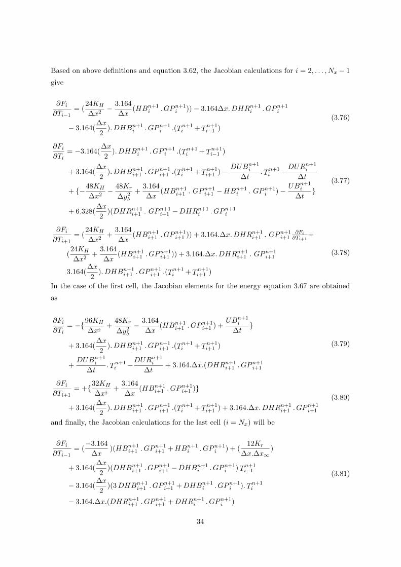
Based on above definitions and equation 3.62, the Jacobian calculations for i = 2, . . . , Nx − 1
give
∂Fi∂Ti−1
= (24KH
∆x2− 3.164
∆x(HBn+1
i . GPn+1i ))− 3.164∆x.DHRn+1
i . GPn+1i
− 3.164(∆x
2). DHBn+1
i . GPn+1i .(T
n+1i +T
n+1i−1 )
(3.76)
∂Fi∂Ti
= −3.164(∆x
2). DHBn+1
i . GPn+1i .(T
n+1i +T
n+1i−1 )
+ 3.164(∆x
2). DHBn+1
i+1 . GPn+1i+1 .(T
n+1i +T
n+1i+1 )−
DUBn+1i
∆t. T
n+1i −
DURn+1i
∆t
+ {−48KH
∆x2− 48Kr
∆y2b
+3.164
∆x(HBn+1
i+1 . GPn+1i+1 −HB
n+1i . GPn+1
i )−UBn+1
i
∆t}
+ 6.328(∆x
2)(DHRn+1
i+1 . GPn+1i+1 −DHR
n+1i . GPn+1
i
(3.77)
∂Fi∂Ti+1
= (24KH
∆x2+
3.164
∆x(HBn+1
i+1 . GPn+1i+1 )) + 3.164.∆x.DHRn+1
i+1 . GPn+1i+1
∂Fi∂Ti+1
+
(24KH
∆x2+
3.164
∆x(HBn+1
i+1 . GPn+1i+1 )) + 3.164.∆x.DHRn+1
i+1 . GPn+1i+1
3.164(∆x
2). DHBn+1
i+1 . GPn+1i+1 .(T
n+1i +T
n+1i+1 )
(3.78)
In the case of the first cell, the Jacobian elements for the energy equation 3.67 are obtained
as
∂Fi∂Ti
= −{96KH
∆x2+
48Kr
∆y2b
− 3.164
∆x(HBn+1
i+1 . GPn+1i+1 ) +
UBn+1i
∆t}
+ 3.164(∆x
2). DHBn+1
i+1 . GPn+1i+1 .(T
n+1i +T
n+1i+1 )
+DUBn+1
i
∆t. T
n+1i −
DURn+1i
∆t+ 3.164.∆x.(DHRn+1
i+1 . GPn+1i+1
(3.79)
∂Fi∂Ti+1
= +{32KH
∆x2+
3.164
∆x(HBn+1
i+1 . GPn+1i+1 )}
+ 3.164(∆x
2). DHBn+1
i+1 . GPn+1i+1 .(T
n+1i +T
n+1i+1 ) + 3.164.∆x.DHRn+1
i+1 . GPn+1i+1
(3.80)
and finally, the Jacobian calculations for the last cell (i = Nx) will be
∂Fi∂Ti−1
= (−3.164
∆x)(HBn+1
i+1 . GPn+1i+1 +HBn+1
i . GPn+1i ) + (
12Kr
∆x.∆x∞)
+ 3.164(∆x
2)(DHBn+1
i+1 . GPn+1i+1 −DHB
n+1i . GPn+1
i )Tn+1i−1
− 3.164(∆x
2)(3DHBn+1
i+1 . GPn+1i+1 +DHBn+1
i . GPn+1i ). T
n+1i
− 3.164.∆x.(DHRn+1i+1 . GP
n+1i+1 +DHRn+1
i . GPn+1i )
(3.81)
34

∂Fi∂T i
= {(3.164
∆x)(3HBn+1
i+1 . GPn+1i+1 −HB
n+1i . GPn+1
i )− (36Kr
∆x.∆x∞)− (
48Kr
∆y2b
)−UBn+1
i
∆t}
− 3.164(∆x
2)(3DHBn+1
i+1 . GPn+1i+1 +DHBn+1
i . GPn+1i ). T
n+1i−1
+ {3.164(∆x
2)(9DHBn+1
i+1 . GPn+1i+1 −DHB
n+1i . GPn+1
i )−DUBn+1
i
∆t}. Tn+1
i
+ 3.164.∆x.(3DHRn+1i+1 . GP
n+1i+1 −DHR
n+1i . GPn+1
i )−DURn+1
i
∆t(3.82)
35

3.7 Summary of The First Model
Figure 3.5: The First Model Calculations Flow Chart
36

4 Second Model
In this model, the pressure will be solved implicitly and after finding the pressure solution,
saturation values can be determined explicitly. This technique is called IMPES and is much
used in the oil industry [8]. During one time step the results of IMPES are used in the tem-
perature equation which is solved fully implicitly, and finally there will a coupling between
the IMPES technique and the fully implicit temperature equation in order to find the final
pressure, saturation and temperature distribution results.
4.1 IMPES Technique
In the oil and water system, the general 3D equations for oil and water are
⇀∇ .(ρo
Koµo~∇Po
)+ ρoΣqo
1.127Vb= 1
6.328∂∂t (ρoϕSo)
⇀∇ .(ρw
Kwµw
~∇Pw)
+ ρwΣqw1.127Vb
= 16.328
∂∂t (ρwϕSw)
(4.1)
By considering the assumptions made in section 2.1 , and considering that generation and
consumption terms are replaced by boundary conditions and expansion of right hand side of
the equations, we have
∂∂x
(ρo
Koµo
∂P∂x
)= ϕ
6.328
[(1− S) ρ′op
∂P∂t + (1− S) ρ′oT
∂T∂t − ρo
∂S∂t
]∂∂x
(ρw
Kwµw
∂P∂x
)= ϕ
6.328
[S ρ′wp
∂P∂t + S ρ′wT
∂T∂t − ρw
∂S∂t
] (4.2)
Divide oil pressure equation by ρo and water pressure equation by ρw , then add them together,
and rearrange the final equation to find the discretized pressure equation for internal cells
(i = 2, . . . , Nx − 1 ), giving
1
ρo
∂
∂x
(ρoKo
µo
∂P
∂x
)+
1
ρw
∂
∂x
(ρwKw
µw
∂P
∂x
)=
ϕ
6.328
[(1− S)
ρ′opρo
+ Sρ′wpρw
]∂P
∂t+
ϕ
6.328
[(1− S)
ρ′oTρo
+ Sρ′wTρw
]∂T
∂t
(4.3)
37

For simplicity we define the equations parameters and terms to be similar to those defined
in the first model (refer to section 3.2). The above equation 4.3 is discretized using a fully
implicit scheme and by considering pressures as the main variables as follows,
(Dn+1oi
ρoi+Dn+1wi
ρwi)P
n+1i−1 −{
Dn+1oi +D
n+1oi+1
ρoi+Dn+1wi +D
n+1wi+1
ρwi+ϕ(1− Sni )
6.328∆t(ρ′opiρoi
) +ϕSni
6.328∆t(ρ′wpiρwi
)}Pn+1i
+ (Dn+1oi+1
ρoi+Dn+1wi+1
ρwi)P
n+1i+1 = −{ϕ(1− Sni )
6.328∆t(ρ′opiρoi
) +ϕSni
6.328∆t(ρ′wpiρwi
)}Pni +
ϕ(1− Sni )
6.328∆t(ρ′oT iρoi
) +ϕSni
6.328∆t(ρ′wT iρwi
)}(Tn+1i −Tni )
(4.4)
Different treatments are required to obtain the pressure equation for the left boundary cell
(i = 1), by considering its boundary conditions (refer to section 2.4).
1
ρoi.∆x{(ρo
Ko
µo
∂P
∂x)i+ 1
2− (ρo
Ko
µo
∂P
∂x)bl}+
1
ρwi∆x{(ρw
Kw
µw
∂P
∂x)i+ 1
2− (ρw
Kw
µw
∂P
∂x)bl}
=ϕ
6.328
[(1− S)
ρ′opρo
+ Sρ′wpρw
]∂P
∂t+
ϕ
6.328
[(1− S)
ρ′oTρo
+ Sρ′wTρw
]∂T
∂t
(4.5)
By using equation 3.30 for the pressure gradient on this boundary,
− {Dn+1oi+1
ρoi+Dn+1wi+1
ρwi+ϕ(1− Sni )
6.328∆t(ρ′opiρoi
) +ϕSni
6.328∆t(ρ′wpiρwi
)}Pn+1i
+ (Dn+1wi+1
ρwi+Dn+1oi+1
ρoi)P
n+1i+1 = −GPI.∆x.(D
n+1oi
ρoi+Dn+1wi
ρwi)
− {ϕ(1− Sni )
6.328∆t(ρ′opiρoi
) +ϕSni
6.328∆t(ρ′wpiρwi
)}Pni +
{ϕ(1− Sni )
6.328∆t(ρ′oT iρoi
) +ϕSni
6.328∆t(ρ′wTiρwi
)}(Tn+1i −Tni )
(4.6)
The investigation for the right boundary cell (i = Nx) shows that
1
ρoi∆x{(ρo
Ko
µo
∂P
∂x)n+1br − (ρo
Ko
µo
∂P
∂x)n+1i− 1
2
}+1
ρwi∆x{(ρw
Kw
µw
∂P
∂x)n+1br − (ρw
Kw
µw
∂P
∂x)n+1i− 1
2
=
ϕ
6.328
[(1− S)
ρ′opρo
+ Sρ′wpρw
]∂P
∂t+
ϕ
6.328
[(1− S)
ρ′oTρo
+ Sρ′wTρw
]∂T
∂t
(4.7)
By using equation 3.32 as the pressure gradient on this boundary and the oil and water
properties at boundary which are calculated from extrapolated temperature and saturation,
and using all these definitions, the discretized pressure equation for i = Nx is
38

(Dn+1oi
ρoi+Dn+1wi
ρwi)P
n+1i −{D
n+1oi
ρoi+Dn+1wi
ρwi+ϕ(1− Sni )
6.328∆t(ρ′opiρoi
) +ϕSni
6.328∆t(ρ′wpiρwi
)}Pn+1i =
GPO.∆x.(Dn+1oi+1
ρoi+Dn+1wi+1
ρwi)− {ϕ(1− Sni )
6.328∆t(ρ′opiρoi
) +ϕSni
6.328∆t(ρ′wpiρwi
)}Pni
− {ϕ(1− Sni )
6.328∆t(ρ′oT iρoi
) +ϕSni
6.328∆t(ρ′wTiρwi
)}(Tn+1i −Tni )
− {ϕ(1− Sni )
6.328∆t(ρ′oT iρoi
) +ϕSni
6.328∆t(ρ′wTiρwi
)}(Tn+1i −Tni )
(4.8)
The result of writing the pressure equation for all blocks is also a nonlinear system to solve,
so the definition of the Jacobian for this system is required.
4.2 Jacobian Calculations for the Pressure Equation
The general equation 4.4 is a function of three variables; Pi−1, Pi and Pi+1 , therefore the
Jacobian matrix is defined as follow
∂Fi∂Pi−1
=1
2(Dn+1wi
ρwiηn+1wpi +
Dn+1oi
ρoiηn+1opi )(P
n+1i−1 −P
n+1i ) + (
Dn+1oi
ρoi+Dn+1wi
ρwi) (4.9)
∂Fi∂Pi
= {Dn+1oi+1(
1
2
ηn+1opi+1
ρoi−ρ′opiρ2oi
) +Dn+1wi+1(
1
2
ηn+1wpi+1
ρwi−ρ′wpiρ2wi
)}Pn+1i+1
− {Dn+1oi +D
n+1oi+1
ρoi+Dn+1wi +D
n+1wi+1
ρwi+ϕ(1− Sni )
6.328∆t.ρ′opiρoi
+ϕSni
6.328∆t.ρ′wpiρwi}
− {Dn+1oi ηn+1
opi +Dn+1oi+1 η
n+1opi+1
2 ρoi+Dn+1wi ηn+1
wpi +Dn+1wi+1 η
n+1wpi+1
2 ρwi
− (Dn+1oi +D
n+1oi+1)(
ρ′opiρoi
)− (Dn+1wi +D
n+1wi+1)(
ρ′wpiρwi
) +ϕ(1− Sni )
6.328∆t.ρ′′oppi ρoi−(ρ′opi)
2
ρ2oi
+ϕSni
6.328∆t.ρ′′wppi ρwi−(ρ′wpi)
2
ρ2wi
}Pi + {Dn+1oi (
1
2
ηn+1opi
ρoi−ρ′opiρ2oi
) +Dn+1wi (
1
2
ηn+1wpi
ρwi−ρ′wpiρ2wi
)}Pn+1i−1
+ {ϕ(1− Sni )
6.328∆t.ρ′′oppi ρoi−(ρ′opi)
2
ρ2oi
+ϕSni
6.328∆t.ρ′′wppi ρwi−(ρ′wpi)
2
ρ2wi
}Pni
− {ϕ(1− Sni )
6.328∆t.ρ′′opT i ρoi−ρ′opi ρ′oT i
ρ2oi
+ϕSni
6.328∆t.ρ′′wpTi ρwi−ρ′wpi ρ′wTi
ρ2wi
}(Tn+1i −Tni )
(4.10)
∂Fi∂Pi+1
=1
2(Dn+1wi+1
ρwiηn+1wpi+1 +
Dn+1oi+1
ρoiηn+1opi+1)(P
n+1i+1 −P
n+1i ) + (
Dn+1oi+1
ρoi+Dn+1wi+1
ρwi) (4.11)
39

The first cell (i = 1) pressure equation depends on two variables; pi and pi+1 , so
∂Fi∂Pi
= {Dn+1oi+1(
1
2
ηn+1opi+1
ρoi−ρ′opiρ2oi
) +Dn+1wi+1(
1
2
ηn+1wpi+1
ρwi−ρ′wpiρ2wi
)}(Pn+1i+1 −P
n+1i )
− {ϕ(1− Sni )
6.328∆t.ρ′′oppi ρoi−(ρ′opi)
2
ρ2oi
+ϕSni
6.328∆t.ρ′′wppi ρwi−(ρ′wpi)
2
ρ2wi
}(Pn+1i −Pni )
− {Dn+1oi+1
ρoi+Dn+1wi+1
ρwi+ϕ(1− Sni )
6.328∆t.ρ′opiρoi
+ϕSni
6.328∆t.ρ′wpiρwi}
+GPI.∆x.{Dn+1oi .(
3
2
ηn+1opi
ρoi− ρ′opi
ρ2oi
) +Dn+1wi .(
3
2
ηn+1wpi
ρwi− ρ′wpi
ρ2wi
)}
+3
2.GPI.∆x.(
Dn+1oi
ρoi+Dn+1wi
ρwi)(µ′wpbµwb
)
− {ϕ(1− Sni )
6.328∆t.ρ′′opT i ρoi−ρ′opi ρ′oT i
ρ2oi
+ϕSni
6.328∆t.ρ′′wpTi ρwi−ρ′wpi ρ′wTi
ρ2wi
}(Tn+1i −Tni )
(4.12)
∂F i∂P i+1
=1
2(Dn+1wi+1
ρwiηn+1wpi+1 +
Dn+1oi+1
ρoiηn+1opi+1)(P
n+1i+1 −P
n+1i ) + (
Dn+1oi+1
ρoi+Dn+1wi+1
ρwi)
− 1
2GPI.∆x.{Dn+1
oi .(ηn+1opi
ρoi) +D
n+1wi .(
ηn+1wpi
ρwi)− 1
2.GPI.∆x.(
Dn+1oi
ρoi+Dn+1wi
ρwi)(µ′wpbµwb
)
(4.13)
and finally, for the last cell (i = Nx) pressure equation which is function of pi and pi−1, we
have;
∂Fi∂Pi−1
=1
2(Dn+1wi
ρwiηn+1wpi +
Dn+1oi
ρoiηn+1opi )(P
n+1i−1 −P
n+1i ) + (
Dn+1oi
ρoi+Dn+1wi
ρwi)
+1
2GPO.∆x(
Dn+1wi+1
ρwiηn+1wpi+1 +
Dn+1oi+1
ρoiηn+1opi+1)
(4.14)
∂Fi∂Pi
= {Dn+1oi (
1
2
ηn+1opi
ρoi−ρ′opiρ2oi
) +Dn+1wi (
1
2
ηn+1wpi
ρwi−ρ′wpiρ2wi
)} (Pn+1i−1 −P
n+1i )
ϕ(1− Sni )
6.328∆t.ρ′′oppi ρoi−(ρ′opi)
2
ρ2oi
+ϕSni
6.328∆t.ρ′′wppi ρwi−(ρ′wpi)
2
ρ2wi
}(Pn+1i −Pni )
− {Dn+1oi
ρoi+Dn+1wi
ρwi+ϕ(1− Sni )
6.328∆t.ρ′opiρoi
+ϕSni
6.328∆t.ρ′wpiρwi}
−GPO.∆x.{Dn+1oi+1 .(
3
2
ηn+1opi+1
ρoi− ρ′opi
ρ2oi
) +Dn+1wi+1 .(
3
2
ηn+1wpi+1
ρwi− ρ′wpi
ρ2wi
)}
− {ϕ(1− Sni )
6.328∆t.ρ′′opT i ρoi−ρ′opi ρ′oT i
ρ2oi
+ϕSni
6.328∆t.ρ′′wpTi ρwi−ρ′wpi ρ′wTi
ρ2wi
}(Tn+1i −Tni )
(4.15)
40

4.3 Saturation Calculations
Oil and water saturations are evaluated explicitly by using the results of the fully implicit
pressure equation. The following equations are applied to find the saturations
∂
∂x(ρo
Ko
µo
∂P
∂x) =
1
6.328
∂
∂t(ϕρoSo)
∂
∂x(ρw
Kw
µw
∂P
∂x) =
1
6.328
∂
∂t(ϕρwSw)
(4.16)
These equations are discretized as
Dn+1oi+1 .(P
n+1i+1 −P
n+1i )−Dn+1
oi (Pn+1i −Pn+1
i ) =ϕ
6.328{ρn+1
oi . Sn+1oi − ρ
noi S
noi}
Dn+1wi+1 .(P
n+1i+1 −P
n+1i )−Dn+1
wi (Pn+1i −Pn+1
i ) =ϕ
6.328{ρn+1
wi . Sn+1wi − ρ
nwi S
nwi}
(4.17)
Hence, oil and water saturations are calculated for internal cells (i = 2, . . . , Nx) from
Sn+1oi = (
6.328∆t
ϕ ρn+1oi
){Dn+1oi+1 . P
n+1i+1 −(D
n+1oi +D
n+1oi+1)P
n+1i +D
n+1oi . P
n+1i }+ (
ρnoi
ρn+1oi
)Snoi
Sn+1wi = (
6.328∆t
ϕ ρn+1wi
){Dn+1wi+1 . P
n+1i+1 −(D
n+1wi +D
n+1wi+1)P
n+1i +D
n+1wi . P
n+1i }+ (
ρnwi
ρn+1wi
)Snwi
(4.18)
For the first cell (i = 1),
Sn+1oi = (
6.328∆t
ϕ ρn+1oi
){Dn+1oi+1(P
n+1i+1 +P
n+1i ) +GPI.∆x.D
n+1oi }+ (
ρnoi
ρn+1oi
)Snoi
Sn+1wi = (
6.328∆t
ϕ ρn+1wi
){Dn+1wi+1(P
n+1i+1 +P
n+1i ) +GPI.∆x.D
n+1wi }+ (
ρnwi
ρn+1wi
)Snwi
(4.19)
and finally for the right boundary cell (i = Nx)
Sn+1oi = −(
6.328∆t
ϕ ρn+1oi
){Dn+1oi (P
n+1i −Pn+1
i−1 ) +GPO.∆x.Dn+1oi+1}+ (
ρnoi
ρn+1oi
)Snoi
Sn+1wi = −(
6.328∆t
ϕ ρn+1wi
){Dn+1wi (P
n+1i −Pn+1
i−1 ) +GPO.∆x.Dn+1wi+1}+ (
ρnwi
ρn+1wi
)Snwi
(4.20)
This is the whole procedure of the IMPES method for this model.
In summary, in this model pressure and saturations are calculated from the IMPES tech-
nique, but a similar method (fully implicit method) with the first model is used to find the
temperature distribution.
41

4.4 Summary of the Second Model
Figure 4.1: The Second Model Calculations Flow Chart
42

5 Results
It is interesting to see the results of the two different numerical techniques applied to a physical
process and to see how choosing between these different techniques can change the results using
the same inputs. Table 1 shows the values of the model parameters used in the two models.
5.1 First Model Results
In this model, the Buckley-Leverett equation and mass and energy balance equations are
solved using the Lax-Wendroff scheme and a fully implicit central schemes, respectively, in
order to find saturation, pressure and temperature distribution in the one dimensional hot
water model. The results for pressure, saturation and temperature profiles are shown in figure
5.1 using a step size of 4x = 5(ft) and a time step of 4t = 0.025(day). Distributions are plot-
ted after 100, 250 and 400 days. It can be seen from figure 5.1 (the water saturation profile)
that initially there is no steep front in the system but later, due to injection a shock (water
front) is created which moves to the right in time. The pressure profile changes based on the
water and oil properties and shock position. Surprisingly, there are no oscillations around
the discontinuity (water saturation front) although the second order accurate Lax-Wenderoff
scheme is used to solve Buckley-Leverett equation. Figure 5.2 shows that with higher number
of divisions the front is steeper, as expected, but still no oscillation is observed around this
steep front. This behavior might be related to using Lax-Wendroff for unequal spacing and
backward in space and forward in time schemes at the boundaries or front is not steep enough.
5.2 Second Model Results
The fully implicit pressure explicit saturation (IMPES) and fully implicit temperature tech-
niques are used to find pressure, saturation and temperature profiles in this model. Results
are presented in figure 5.3 by using similar step sizes and time steps to the first model. The
results show that there are similar trend for outputs.
43
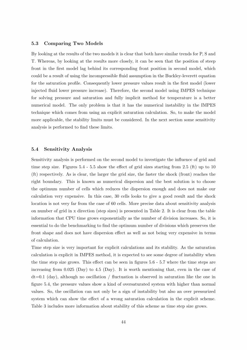
5.3 Comparing Two Models
By looking at the results of the two models it is clear that both have similar trends for P, S and
T. Whereas, by looking at the results more closely, it can be seen that the position of steep
front in the first model lag behind its corresponding front position in second model, which
could be a result of using the incompressible fluid assumption in the Buckley-leverett equation
for the saturation profile. Consequently lower pressure values result in the first model (lower
injected fluid lower pressure increase). Therefore, the second model using IMPES technique
for solving pressure and saturation and fully implicit method for temperature is a better
numerical model. The only problem is that it has the numerical instability in the IMPES
technique which comes from using an explicit saturation calculation. So, to make the model
more applicable, the stability limits must be considered. In the next section some sensitivity
analysis is performed to find these limits.
5.4 Sensitivity Analysis
Sensitivity analysis is performed on the second model to investigate the influence of grid and
time step size. Figures 5.4 - 5.5 show the effect of grid sizes starting from 2.5 (ft) up to 10
(ft) respectively. As is clear, the larger the grid size, the faster the shock (front) reaches the
right boundary. This is known as numerical dispersion and the best solution is to choose
the optimum number of cells which reduces the dispersion enough and does not make our
calculation very expensive. In this case, 30 cells looks to give a good result and the shock
location is not very far from the case of 60 cells. More precise data about sensitivity analysis
on number of grid in x direction (step sizes) is presented in Table 2. It is clear from the table
information that CPU time grows exponentially as the number of division increases. So, it is
essential to do the benchmarking to find the optimum number of divisions which preserves the
front shape and does not have dispersion effect as well as not being very expensive in terms
of calculation.
Time step size is very important for explicit calculations and its stability. As the saturation
calculation is explicit in IMPES method, it is expected to see some degree of instability when
the time step size grows. This effect can be seen in figures 5.6 - 5.7 where the time steps are
increasing from 0.025 (Day) to 4.5 (Day). It is worth mentioning that, even in the case of
dt=0.1 (day), although no oscillation / fluctuation is observed in saturation like the one in
figure 5.4, the pressure values show a kind of oversaturated system with higher than normal
values. So, the oscillation can not only be a sign of instability but also an over pressurized
system which can show the effect of a wrong saturation calculation in the explicit scheme.
Table 3 includes more information about stability of this scheme as time step size grows.
44
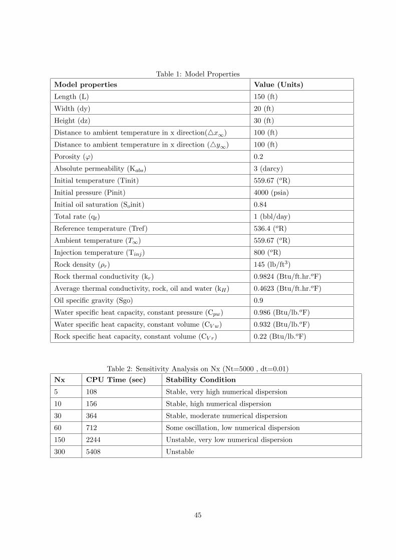
Table 1: Model Properties
Model properties Value (Units)
Length (L) 150 (ft)
Width (dy) 20 (ft)
Height (dz) 30 (ft)
Distance to ambient temperature in x direction(4x∞) 100 (ft)
Distance to ambient temperature in x direction (4y∞) 100 (ft)
Porosity (ϕ) 0.2
Absolute permeability (Kabs) 3 (darcy)
Initial temperature (Tinit) 559.67 (oR)
Initial pressure (Pinit) 4000 (psia)
Initial oil saturation (Soinit) 0.84
Total rate (qt) 1 (bbl/day)
Reference temperature (Tref) 536.4 (oR)
Ambient temperature (T∞) 559.67 (oR)
Injection temperature (Tinj) 800 (oR)
Rock density (ρr) 145 (lb/ft3)
Rock thermal conductivity (kr) 0.9824 (Btu/ft.hr.oF)
Average thermal conductivity, rock, oil and water (kH) 0.4623 (Btu/ft.hr.oF)
Oil specific gravity (Sgo) 0.9
Water specific heat capacity, constant pressure (Cpw) 0.986 (Btu/lb.oF)
Water specific heat capacity, constant volume (CV w) 0.932 (Btu/lb.oF)
Rock specific heat capacity, constant volume (CV r) 0.22 (Btu/lb.oF)
Table 2: Sensitivity Analysis on Nx (Nt=5000 , dt=0.01)
Nx CPU Time (sec) Stability Condition
5 108 Stable, very high numerical dispersion
10 156 Stable, high numerical dispersion
30 364 Stable, moderate numerical dispersion
60 712 Some oscillation, low numerical dispersion
150 2244 Unstable, very low numerical dispersion
300 5408 Unstable
45

Table 3: Sensitivity Analysis on dt (Nx=30 , Final time=50 Day)
Nx CPU Time (sec) Stability Condition
0.01 364 Stable
0.05 76 Stable
0.1 36 No oscillation, over-saturated
0.5 8 No oscillation, over-saturated
1 8 Some oscillation
2 8 More oscillation
5 – Nearly singular matrix - no result
46

Figure 5.1: The First Model Pressure, Saturation and Temperature Results
47

Figure 5.2: The First Model Pressure, Saturation and Temperature Results , Nx=300
48

Figure 5.3: The Second Model Pressure, Saturation and Temperature Results
49

Figure 5.4: Pressure, Saturation and Temperature Profiles for the second model for Nx=15
50

Figure 5.5: Pressure, Saturation and Temperature Profiles for the second model for Nx=60
51

Figure 5.6: The Second Model Pressure, Saturation and Temperature Profiles (dt=0.1 Day)
52

Figure 5.7: The Second Model Pressure, Saturation and Temperature Profiles (dt=4.5 Day)
53

6 Conclusion
In this dissertation two numerical models have been applied to a method of oil recovery, hot
water injection. This physical process can be described using oil and water mass conservation
equations, energy balance and Buckley-Leverett equations. Hot water injection is modeled by
using these equations in order to find pressure, saturation and temperature profiles.
In first model Lax-Wendroff and fully implicit scheme have been used to solve Buckley-
Leverett, oil mass and energy balance equations respectively. The model may be less reli-
able since one of the basic assumptions of Buckley-Leverett equation is considering fluids as
incompressible which is not a reasonable assumption in this study. It is worth noticing that
Lax-Wendroff method is a second order accurate scheme, and it is a well-known fact that
second order accurate numerical schemes produce oscillations at discontinuities, but there are
no oscillations in the saturation profile of this study and the results around shock are smooth.
The reason may be related to, using backward in space and forward in time scheme at right
boundary and Lax-Wendroff based on unequal step size at left boundary.
Implicit pressure explicit saturation (IMPES) and fully implicit energy equation have been
implemented to obtain the distributions in the second model. This technique seems to be more
reliable as it has been driven by considering fluid compressibility which is an effective factor in
thermal processes. However, the explicit saturation calculations make this method sensitive
to stability so, the stability of this model is under question and has to be treated carefully
to get correct results. Sometimes, it seems there is no visual instability in water saturation
profile but saturation can easily be overestimated resulting in over-pressurization of the system.
6.1 Future work
• The model can be easily extended to a two- or three-dimension. There would be similar
trend but calculations would be more expensive.
• Other phenomena such as gravity, capillary pressure, and temperature dependence of
relative permeability can be included in the models which cause higher degree of non-
linearity.
• Other numerical methods can be applied to the set of equations and compare their
54

results with the result of this study. For instance, oil and water mass balance equations
and energy balance equation can be modeled using fully implicit method for all of them
and solve them simultaneously which is a well-known method but, it is really expensive
technique in calculation.
• Using different boundary conditions (well models) to investigate their effect on the sat-
uration, pressure and temperature distributions in the system.
• In first model, other numerical methods like Warming-Beam, Fromm, etc., can be used
to find the saturation in Buckley-Leverett equation.
55

Nomenclature
P Pressure (psia)
V Volume (cu ft)
ρ Density (lbm/cu ft)
u Velocity (ft/days)
g Gravitational acceleration
d Reservoir depth (ft)
x Distance along the x direction (ft)
4x Grid size in x-direction (ft)
4t Grid size in temporal direction (days)
K Permeability (darcy)
Kr Relative permeability (dimensionless)
µ Viscosity (cp)
ϕ Porosity (fraction)
S Saturation (fraction)
APIo Oil gravity measurement
q Flow rate (bbl/days)
A Area (sq ft)
f Fractional fluid flow (dimensionless)
t Time (days)
mo Mass flux (lbm/days)
M Mass (lbm)
E Total rock and fluid energy (Btu/cu ft)
eo Energy flux (Btu/days)
U Internal energy (Btu/lbm)
H Enthalpy (Btu/lbm)
Q Amount of heat (Btu/lbm)
T Temperature (0R)
Cp Heat capacity at constant pressure (Btu/lbm. 0F)
CV Heat capacity at constant volume (Btu/lbm. 0F)
k Thermal conductivity (Btu/hr. ft. 0F)
rw Well radius (ft)
h Reservoir thickness (ft)
X Dimensionless distance
L Distance between injection and production wells (ft)
56

Subscripts and Superscripts
α Phase index (o = oil, w = water)
w Water phase
o Oil phase
b Boundary
c Capillary pressure
abs Absolute
p Pore or Pressure
r Relative or Rock
t Total
prod Production
inj Injection
gen Generation
cons Consumption
V Volume
or Residual oil
wc Connate water
av Average
ref Reference
57

References
[1] Tarek Ahmed, Reservoir Engineering Handbook , Second Edition, Gulf Professional Pub-
lishing, 2001, pp.184-228, 281-286.
[2] R. E. Ewing, The Mathematics of Reservoir Simulation , SIAM, Philadelphia, (1983)
[3] A. T.Corey,The Interrelation Between Gas and Oil Relative Permeabilities , Producers
Monthly, 1954, pp.38-41
[4] www.most.gov.mm/techuni/media/PE 05045 2.pdf.
[5] M.Y. Soliman, W.E. Brigham, Raj Raghavan, Numerical Simulation of Thermal Recovery
Processes , SPE 9942, 1981.
[6] Professor Jon Kleppe, TPG4150 Reservoir Recovery Techniques , Handout notes 4 :
Buckley-Leverett Analysis, Norwegian University of Science and Technology, Department
of Petroleum Engineering and Applied Geology, Sep. 2012.
[7] B.C.Craft, M.Hawkins, Applied Petroleum Reservoir Engineering , Second Edition, Pren-
tice Hall PTR, 1991.
[8] Chen Z.,Huan G.,Ma Y, Computational Methods for Multiphase Flow in Porous Media ,
SIAM Publications, 2006, pp.10-14, 265-267, 382-384.
[9] P.K Sweby,Numerical Solution of Conservation Laws Lecture notes, University of Reading
(2002).
[10] K.W. Morton and D.F. Mayers,Numerical Solution of Partial Differential Equations ,
Cambridge university press, (1994).
[11] H.G. Weinstein, J.A. Wheeler, E.G. Woods, Numerical Model for Thermal Processes ,
SPE 4759, 1974.
[12] Prats, Michael, Thermal Recovery , New York, (1986).
[13] C. T. Kelley, Solving Nonlinear Equations with Newton’s Method, No. 1 in Fundamentals
of Algorithms, SIAM, 2003.
58