Modelling micro:bit sensor data captured with Bluetooth Adrian Oldknow Jan 2nd 2017

Martin Woolley has generously made available free Apps for Android and Apple mobile devices to read and

display data captured from micro:bit sensors in real-time. The current versions of the Bitty Data Logger Apps

are described here.

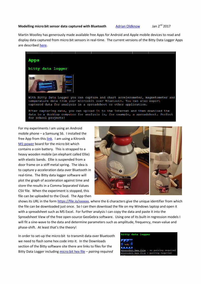
For my experiments I am using an Android

mobile phone – a Samsung S6. I installed the

free App from this link. I am using a Kitronik

M1:power board for the micro:bit which

contains a coin battery. This is strapped to a

heavy wooden mobile (an elephant called Ellie)

with elastic bands. Ellie is suspended from a

door frame on a stiff metal spring. The idea is

to capture y-acceleration data over Bluetooth in

real-time. The Bitty data logger software will

plot the graph of acceleration against time and

store the results in a Comma Separated Values

CSV file. When the experiment is stopped, this

file can be uploaded to the Cloud. The App then

shows its URL in the form https://file.io/xxxxxx, where the 6 characters give the unique identifier from which

the file can be downloaded just once. So I can then download the file on my Windows laptop and open it

with a spreadsheet such as MS Excel. For further analysis I can copy the data and paste it into the

Spreadsheet View of the free open-source GeoGebra software. Using one of its built-in regression models I

will fit a sine-wave to the data and determine parameters such as amplitude, frequency, mean-value and

phase-shift. At least that’s the theory!

In order to set-up the micro:bit to transmit data over Bluetooth

we need to flash some hex code into it. In the Downloads

section of the Bitty software site there are links to files for the

Bitty Data Logger including micro:bit hex file – pairing required

and micro:bit hex file – no pairing required. Download one of these and flash

it to your micro:bit. The PXT version of the program is shown alongside. The

Bitty site has an excellent collection of videos and guides to help you

understand what to do and what is going on. The program enables Bluetooth

connections for the micro:bit’s accelerometers, magnetometers and

temperature sensors and detects whether or not it is connected to a

Bluetooth device. The first time it is run it will ask you to “draw a circle” using

a single flashing led. When you have completed a large letter “O” it will show

a smiley face to let you know the magnetometers have been calibrated. Once you have the code flashed and

running (and, if necessary, completed the pairing) then the Bitty software is all set to go.

Using the Scan tab you can see which (of possibly many)

micro:bits the App can detect. When you tap on the one you

want it will connect to it, and the letter “C” should appear on

the micro:bit to let you know that the connection was

successful. Using the Options tab you can set up the sensors

you want to use, as well as the sampling rate. I have

selected just the Y accelerometer, with a rate of 50 readings

per second. Now everything is set up for the experiment, so

return to the main screen using Back, and then press the

green Start button on the screen.

The blue graph is showing that accelerations are

varying smoothly around a mean value of about 1 –

which is what should be expected since the units of

the values of acceleration returned are multiples of

the acceleration due to gravity g. When you have a

few clear waves, press the red Stop button on the

screen.

If you now select the Results tab you will see a list

of recent CSV files. Tap on the most recent file to

see information about it. Tap on the Upload tab to

send it to the Cloud. Now you have the URL you

need to download the CSV file on whatever device

you want to use for the data analysis:

https://file.io/nb6R9K .

Opening the CSV file on my Windows laptop takes it

straight into MS Excel. I have deleted the first few

lines of information. If you scroll down the sheet you

will see that after the accelerometer data there are

further data sets from the magnetometer and the

temperature sensors, so I have deleted these

unwanted rows. You will also see that there are

columns of data for the X and Z accelerations, so I

have deleted them as well. So the lean and mean

version of the spreadsheet now just has two columns,

from which I can draw a scattergraph. Excel has an

option to `add a trend-line’ which could be linear,

polynomial, power or exponential – but does not

include a sine-wave. So we can copy the data from

the A and B columns and paste them into columns of a

Spreadsheet View in the free GeoGebra software.

Column C is just column A divided by 1000 to convert times into seconds, and D is just a copy of B. Selecting

C and D we can carry out a 2-variable regression analysis of acceleration against time, and select `sin’ as the

regression model. A scattergram is drawn and we can see that a sine-wave gives a very good fit to the data.

The mean value of 1.03 is very close to expected value of 1 (at rest the vertical acceleration would just be 1g

ms-2 downwards.) We can also see that the amplitude of the oscillations is 0.13g ms-2 and that the period is

2π/4.19 or about 1.5 seconds. There is also a phase shift of 0.28.

For a more sophisticated approach we could simultaneously collect displacement data for Ellie. It would be

nice if we could attach a distance sensor – and I am sure that this can happen soon! In the meantime we can

use a video clip of the experiment to capture distances. I have used Blue-Tack to attach the micro:bit to the

base of Ellie and facing down – so this time we

need to set up the Bitty Data Logger to capture z-

accelerations. I have also mounted a digital

camera on a tripod lined up with Ellie at rest. This

will take video clips at 30 frames per second and

save them in the AVI video format.

At the same time as Ellie is released and the Bitty

Data Logger starts recording z-accelerations, my

assistant starts the camera recording a video of

the motion. We both stop recording after we

have a few clear oscillations. The resulting

acceleration data is stored as a CSV file and

uploaded to the cloud, from where we can open it

in Excel, as before.

The time in milliseconds is in column A. The z-

acceleration data has been copied to column C.

The times have been divided by 1000 in column B

to give the time in seconds. A scatterplot of z

against t has had a trend-line drawn – as a linear

fit. From which we can see that the mean value of

acceleration is again slightly over-estimated as

1.03g. Column D is just a copy of column B and

column E is the accelerations in column C with the

mean value of 1.03 subtracted. The scatter-plot of

z1 against t1 shows a decent approximation to a

sine-wave for changes in acceleration. Now we

swop software from Excel to the free Tracker video software for physics. Dr. Tony Houghton and I have

produced a MOOC to show how to extract position data from a video clip and to analyse it in GeoGebra.

The AVI file has been copied from my camera to my Windows laptop, and opened in Tracker.

The blue measuring stick is set to the distance from Ellie’s base to the bottom of the spring, which has been

measured as 0.23m. Axes have been selected and dragged so we can measure displacements from a

suitable base-line (which can be easily adjusted). The AVI clip is marked with its frame rate (30 fps) so

Tracker already has a `clock’ for the timing of each frame. We just need to mark the position of a chosen

feature of Ellie as she oscillates. I have chosen to `auto-track’ her left eye which has a distinctive black and

white pattern. The t, x and y coordinates of the trace are automatically stored in the Table for mass A. I

have also asked Tracker to numerically estimate velocity vy and acceleration ay data from the y and t values.

The 3 graphs show that each has a similar form. As you step through the video you can see which row of

data corresponds to the current frame, and see

the corresponding points on each graph. You can

carry out analysis in Tracker itself. I have

exported the data as a CSV file which we can open

in Excel. The scatterplot of y against t is shown.

We can now copy the data starting from row 5

down to the last row for which an acceleration

has been computed. Then we can paste this into

a GeoGebra spreadsheet view, as before.

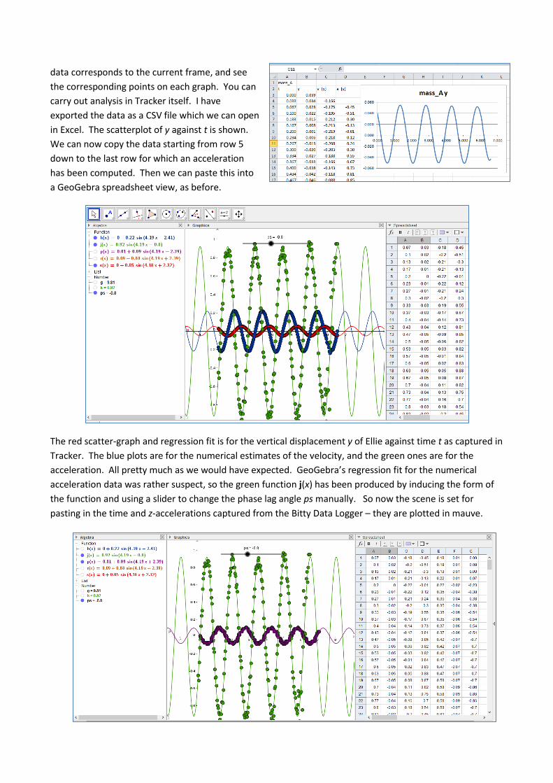
The red scatter-graph and regression fit is for the vertical displacement y of Ellie against time t as captured in

Tracker. The blue plots are for the numerical estimates of the velocity, and the green ones are for the

acceleration. All pretty much as we would have expected. GeoGebra’s regression fit for the numerical

acceleration data was rather suspect, so the green function j(x) has been produced by inducing the form of

the function and using a slider to change the phase lag angle ps manually. So now the scene is set for

pasting in the time and z-accelerations captured from the Bitty Data Logger – they are plotted in mauve.

At first sight this seems to be a disaster! The mauve Bitty accelerations seem to be a factor of about 10

smaller than the green Tracker ones – but why? The answer is in the units. The Tracker accelerations are in

ms-2, whereas the Bitty ones are in multiples of g – which is nearly 10 ms-2. So if we rescale the Bitty

accelerations by multiplying by 9.81 we can see that we are indeed now on the same wavelength!

Column G is just the net accelerations in column F multiplied by g = 9.81. The corrected accelerations from

Bitty are shown in brown. All is now nearly as the physics would have predicted. Certainly the brown and

red functions intersect on the x-axis as expected. But we would also expect the accelerations to be negative

when the velocities are decreasing, and positive when they are increasing. That reminds us that we should

have multiplied F values by –g rather than +g,

since the acceleration due to gravity is actually -

9.81 ms-2.

The final relationships between the models for

micro:bit acceleration data in green, the Tracker

displacement data in red and the Tracker

estimates for velocity in blue are shown clearly

in the GeoGebra graphs of Ellie’s oscillations.

I hope this has given something of the flavour of

how scientific and engineering experiments can

be easily measured using micro:bit’s on-board

sensors, possibly enhanced with other devices.

And how powerful free software tools such as

Tracker and GeoGebra can used to analyse and

model the data mathematically. It is quite

amazing that about £15 not only buys you an

impressive array of sensors, but also the whole

micro:bit with its ARM mBed processor and BlueTooth Low Energy transmission.