modelling ‘evo-devo’ with rna

Modelling ‘evo-devo’ with RNAWalter Fontana

SummaryThe folding of RNA sequences into secondary structuresis a simple yet biophysically grounded model of agenotype–phenotype map. Its computational and math-ematical analysis has uncovered a surprisingly richstatistical structure characterized by shape space cover-ing, neutral networks and plastogenetic congruence. Ireview these concepts and discuss their evolutionaryimplications. BioEssays 24:1164–1177, 2002.� 2002 Wiley Periodicals, Inc.

Introduction

Phenotype refers to the physical, organizational and beha-

vioral expression of an organism during its lifetime. Genotype

refers to a heritable repository of information that instructs

the production ofmoleculeswhose interactions, in conjunction

with the environment, generate and maintain the phenotype.

The processes linking genotype to phenotype are known as

development. They intervene in the genesis of phenotypic

novelty from genetic mutation. Evolutionary trajectories there-

fore depend on development. In turn, evolutionary proces-

ses shape development, creating a feed-back known as ‘‘evo-

devo’’.(1,2)

The main thrust of this review is to show that some key

aspects of this feedback are present even in the microcosm

of RNA folding. In a narrow sense, the relation between RNA

sequences and their shapes is treated as a problem in bio-

physics. Yet, in awider sense,RNA folding can be regardedas

a minimal model of a genotype–phenotype relation.(3)

The RNA model is not a representation of organismal de-

velopment. The regulatory networks of gene expression and

signal transduction that coordinate the spatiotemporal unfold-

ing of complex molecular processes in organismal devel-

opment (for recent overviews see Refs. 4,5) have no concrete

analogue in the RNA sequence-to-structure map. Devel-

opmental processes themselves evolve and this too is out-

side the scope of the rather simple notion of RNA folding

considered here. Yet, the RNA folding map transparently

implements concepts like epistasis and phenotypic plasticity,

thus enabling the study of constraints to variation, canali-

zation, modularity, phenotypic robustness and evolvability.

As detailed in this review, the statistical architecture of the

sequence-to-structure map in RNA offers explanations for

patterns of phenotypic evolution, such as directionality and

the partially punctuated nature of evolutionary change. This

statistical architecture is critically shaped by ‘developmental

neutrality’ that is, the extent towhichmany genotypesmap into

the same phenotype. The RNAmodel is an abstract analogue

of development that grounds a discussion of these issues

within a simple biophysical and formal framework. The fact

that neutrality is a key factor in organizing the genotype-

phenotype relation does not hinge on the nature of develop-

mental mechanisms generating neutrality, but, of course, the

extent of neutrality does. Whether the features present in the

RNA map carry over to more complex genotype–phenotype

maps will depend on the genetic robustness of developmental

mechanisms.

An important purpose of simple and abstract models in

biology is to sharpen the questions—perhaps even to under-

stand what the questions are. In this vein, the RNA model

contributes in making more precise what we mean when we

speak of ‘‘phenotype space’’. Like any other phenotype, an

RNA shape cannot be heritably modified in a direct way, but

requires a change in the underlying sequence. This indirection

in transforming one phenotype into another makes the struc-

ture of phenotype space dependent on the structure of geno-

type space and the mapping from genotype to phenotype.

The absence of a formal theory addressing the latter depen-

dence in the neo-Darwinian school of evolutionary thought

has led to unwarranted assumptions about the structure of

phenotype space and to much confusion about continuity and

discontinuity in evolution (for a discussion see Ref. 6).

RNA phenotypes

Secondary structureRNA structure can be defined at several levels of resolution.

The level known as secondary structure is presently the best

compromise between theoretical tractability and empirical

accessibility on a large scale. The term secondary structure

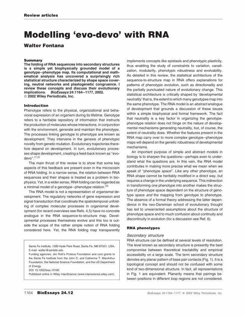
denotes any planar pattern of base pair contacts (Fig. 1). It is a

topological concept and should not be confused with some

kind of two-dimensional structure. In fact, all representations

in Fig. 1 are equivalent. Planarity means that pairings be-

tween positions in different loop regions are not considered.

1164 BioEssays 24.12 BioEssays 24:1164–1177, � 2002 Wiley Periodicals, Inc.

Santa Fe Institute, 1399 Hyde Park Road, Santa Fe, NM 87501, USA.

E-mail: [email protected]

Funding agencies: Jim Rutt’s Proteus Foundation and core grants to

the Santa Fe Institute from the John D. and Catherine T. MacArthur

Foundation, the National Science Foundation, and the US Department

of Energy.

DOI 10.1002/bies.10190

Published online in Wiley InterScience (www.interscience.wiley.com).

Review articles

In the circle representation of Fig. 1B, chords never cross.

The secondary structure repertoire of a sequence consists of

all base pairings that are compatible with the rules A �U, G �Cand G �U.

A secondary structure graph can be uniquely decomposed

into loops and stacks.(7) A stack is a run of adjacent pairs,

corresponding to a double-helical arrangement in the three-

dimensional structure. A loop consists of varying numbers of

unpaired bases and stacks that originate from it (Fig. 1A). The

major stabilizing free energy contribution comes from stacking

interactions between adjacent base pairs. The G �C/G �Cstacking interaction is roughly 3(2) times the A �U/A�U(A �U/G �C) interaction.(8) Loops, in contrast, are destabilizing. The

formation of a stack necessarily causes the formation of a

loop. This ‘‘frustrated’’ energetics can generate a very rugged

energy landscape over the secondary structure space of a

given sequence. Because the energetically relevant units are

loops and stacks rather than individual base pairs, a structure

that minimizes free energy is oftentimes unique and quite

different from one that maximizes the base pair count. For

example, the 77nucleotide histidine tRNAhis (EMBLaccession

RH1660) has one minimum free energy secondary structure

(22basepairs) and149,126 secondary structures realizing the

maximum of 26 base pairs.(9)

The free energy contributions of stack and loop elements

have been empirically determined.(8,10–13) Combinatorial

algorithms,(7,14–16) based on a powerful optimization techni-

que known as dynamic programming,(17) reference these

parameters when computing the minimum free energy stru-

cture of a sequence. This procedure, however, does not

consider the dynamical folding process by which a sequence

acquires its structure.

Base pairings that break planarity are called pseudoknots

and are considered to be tertiary structure elements. Thermo-

dynamic(18) and kinetic(19) algorithms that account for pseu-

doknots have been developed recently. Although widespread

in naturally occurring RNAs, pseudoknots will not be consi-

dered here.

The secondary structure participates as a geometric,

kinetic and thermodynamic scaffold(20) in the formation of the

three-dimensional structure, which involves bringing secon-

dary structure elements into proximity by means of pseudo-

knots, non-standard base pairings and bivalent counter

ions. Its correlation with functional properties of the tertiary

Figure 1. RNA secondary structure representa-

tions. A secondary structure is a graph of contacts

between nucleotides at positions i¼1, . . . , n along

the sequence. Position 1 is the 50 end. The graph

has two types of edges: the backbone connecting

nucleotide i with nucleotide iþ1 (red) and hydro-

gen-bonded base pairings between non-adjacent

positions (green). The set of base pairings,P, must

satisfy two conditions: (i) each nucleotide can pair

with atmost one other nucleotide (green edges inAor B) and (ii) pairings cannot cross (this is best

expressed by representation B where chords,

standing for base pairs, are not allowed to

intersect). Condition (ii) expresses (outer) planar-

ity.A: Typical visualization of a structure.B: Circlerepresentation. C: Line-oriented representation.

A dot stands for an unpaired position and a pair of

matching parentheses indicates paired positions.

D: Tree representation. Base pairs are internal

nodes and unpaired positions correspond to

leaves. The top node (square) keeps the tree

rooted for structures with dangling 50 or 30 ends andjoints. (A–D) contain exactly the same structure

information.

Review articles

BioEssays 24.12 1165

structure is evidenced by phylogenetic conservation.(21)

Further details on the biophysical and computational aspects

of RNA secondary structure can be found in several re-

views.(7,22–24)

I will henceforth refer to the (minimum free energy) secon-

dary structure as (mfe) shape. In the following, I will discuss

various notions of phenotype that can be defined and

computed at this level of structure (Fig. 2).

Energy (kinetic) landscapeThermodynamic folding algorithms only map a sequence

into its global mfe shape. In contrast, kinetic algorithms are

concernedwith howa sequence folds and hencewith the rates

and paths through configuration space that constrain and

promote folding.(19,25–28) A sequence may fold reliably into a

shape other than the mfe shape or it may switch between

metastable shapes with a long lifetime relative to the mole-

cule’s interaction time scale.(29,30)

In modelling the folding process, the key concept is the

energy (or kinetic) landscape (Fig. 2A). The configuration

space of the many shapes compatible with a given sequence

is defined in terms of elementary ‘‘moves’’ that interconvert

shapes. The free energy associated with each shape gives

rise to an energy landscape over the configuration space and

the energy differences between adjacent shapes determine

(roughly) the transition probabilities.(19,28,31)

The energy landscape of a sequence is the RNA analogue

of Waddington’s developmental or epigenetic landscape.(32)

Sequences folding into the same mfe shape can differ pro-

foundly in their energy landscapes. In this limited sense, the

RNA model is capable of mimicking an ‘‘evolution of deve-

lopment’’. The analogy breaks down when themechanisms of

development themselves evolve.(33) After all, an RNA sequ-

ence does not code for the base pairing rules.

Phenotypic plasticityA sequence can wiggle between alternative low-energy

shapes as a consequence of energy fluctuations comprising

a few kT (k is the Boltzmann constant and T the absolute

temperature). The phenotypic plasticity of a sequence is

quantified by the probability pij that positions i and j are paired

with one another. The pij are obtained from a calculation of

the partition function,(34) Z¼Si exp(�E(Si)/kT), where E(Si) is

the free energy of shape Si. Fig. 2B depicts a matrix of such

probabilities (upper triangle), compared to a rendering in the

same format of the mfe shape (lower triangle). To further ex-

press plasticity as a single number, the matrix of base pairing

probabilities can be collapsed into an entropy-like quantity.(35)

A useful description of plasticity, to which I shall return

later, is the set of all shapes within a free energy interval of,

say, 5kT (3 kcal/mol at 378C) from thegroundstate(9) (Fig. 2C).

This set is termed the plastic repertoire.(36)

Knowing the partition function Z and assuming thermo-

dynamic equilibration, we compute the fraction of time that

a molecule spends in any shape Si of its plastic repertoire as

p(Si)¼ exp(�E(Si)/kT )/Z. The extent to which the mfe shape

is the most-occupied configuration varies significantly among

sequences.

Plasticity so-defined emphasizes an intrinsic phenotypic

variance, induced bymolecular energy fluctuations at nonzero

temperature. A more traditional use of the term, known as

norm of reaction,(37) refers to persistent phenotypic change

as a function of environmental parameters. The biophysical

analogue in RNA is the melting profile, that is, the suite of mfe

shapes as a function of temperature (Fig. 2D), or its statistical

equivalent, the specific heat (Fig. 2E).

The difference between the two plasticities (intrinsic vari-

ance and norm of reaction) is best understood in terms of

the free energy landscape underlying the folding behavior of

a sequence. The topography of a free energy landscape

depends non-monotonically on the temperature (the environ-

ment). Plasticity understood as a norm of reaction refers to

transitions between mfe shapes as the free energy landscape

is deformed by temperature, while plasticity understood as

intrinsic phenotypic variance refers to transitions between

different shapes on a fixed free energy landscape.

Loop-structureA shape can be coarse-grained by disregarding the size of

loops and the length of stacks, retaining only the relative

arrangements of loops (Fig. 2F). This skeletal morphology will

be referred to as loop-structure.

Interaction phenotypesBase pairs may be formed within or between molecules.

Straightforward extensions of standard thermodynamic and

kinetic folding algorithms yield the joint shape acquired by

two (or more) sequences.(22) This defines a natural notion

of interaction (Fig. 2G) which could form the basis for RNA

models of coevolution.

Neutrality, epistasis, canalization

I begin with some terminology. Sequences that differ from a

reference sequence by n point mutations are called n-error

neighbors. A neutral mutation is a nucleotide substitution that

preserves the mfe shape (but it may affect everything else,

such as free energy, plastic repertoire and kinetic landscape).

A one-error neighbor that preserves the same mfe shape is

termed a neutral neighbor. A sequence position that allows

for at least one neutral mutation is termed a neutral position

(Fig. 3). The neutrality of a sequence is the fraction of neutral

(one-error) neighbors.

Neutrality is here defined with respect to mfe shape, not

fitness. Fitness is a function from phenotypes to numbers and

if phenotype is defined as mfe shape, then neutrality extends

Review articles

1166 BioEssays 24.12

to fitness as well. If phenotype and fitness are defined in terms

of the plastic repertoire of a sequence, I shall still refer to

sequences that share the same mfe shape as neutral, even

when their plastic repertoires (and fitness) differ.

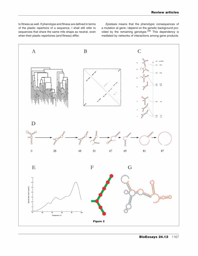
Epistasis means that the phenotypic consequences of

a mutation at gene i depend on the genetic background pro-

vided by the remaining genotype.(38) This dependency is

mediated by networks of interactions among gene products.

Figure 2

Review articles


The same concept applies to RNA, when substituting ‘‘gene’’

with ‘‘sequence position’’. The transparency (but also the

limitation) of the RNA genotype–phenotype model derives

from the identity of epigenetic and epistatic interactions, since

phenotype is defined directly in terms of interactions among

sequence positions.

A mutation changes the base pairing possibilities of a

sequence and hence the network of epistatic interactions.

Themfe shape shown at the top left of Fig. 3 remains the same

if C is substituted byG at the position labelled x. Yet, whether x

is C or G determines which mfe shape is obtained as a result

of mutating position y from G to A. More subtly, the neutral

substitution from C to G at x alters the number and identity of

neutral positions.

The tendency of a sequence to adopt a different shape

upon mutation (variability) is a prerequisite for its capacity

Figure 2. RNA phenotypes. All examples refer to the sequence of Fig. 1. A: Developmental landscape. The graph shows the barrier-

tree28 of the low-energy portion of the free energy landscape. The barrier tree depicts the likelihood of a conversion from one shape

configuration into another. This is how it should be read. The vertical dimensionmeans free energy. The leaves of the tree are shapes (not

shown) that correspond to local energyminimaand thehighest point on the route fromoneminimum toanyother indicates theenergybarrier

that controls the likelihoodof that route. The likelihood (at constant temperature) of switching betweenany two configurations is exponential

in the (negative) height of that barrier.Highbarriersmeanvery longcrossing times (or lowcrossingprobabilities). Thestructureof this barrier

landscape determines the folding paths and rates.B: Thematrix of base-pairing probabilities. The size of a dot at location (i, j) in the upper

triangle depicts the probability that position i is paired with position j (i< j ). For comparison, the lower triangle displays the pairing pattern of

the mfe shape. While the mfe pattern is predominant in the upper triangle, dots of significant size exist at alternative positions, indicating

different folds.C:Plastic repertoire. Theset of shapeswithin 5 kT (3 kcal/mol at 378C) from themfe shape.Only a fewshapesare shownand

their relative energy is indicated on the vertical bar whose total length corresponds to 3 kcal/mol.D:Norm of reaction I (melting profile). The

seriesofmfe shapes is shownas the temperature is raised from08C to the temperatureatwhich this sequence losesall secondarystructure.

E:Normof reaction II (specific heat). The specific heat is given byH¼�Td2G/dT 2withG¼�RT logZ (G is theGibbs free energy,R the gas

constant, T the absolute temperature and Z the partition function). H profiles the changes in the statistical weights of the shape

configurations available to an RNA sequence as the temperature is raised. The humps in the specific heat indicate the major melting

transitions at 288, 488, 678 and 878 shown in D. This function can be measured by differential scanning calorimetry. F: Loop structure: the

relative arrangement of loops disregarding the size of stacks and loops.G: Joint shape of two hybridized RNA sequences.

Figure 3. Epistasis. Bullets indicate a neutral posi-

tion. In the top left sequence, position x is neutral

because the substitution of G for C preserves the

shape, as shown at the top on the right. Yet, neutral

positions do change as a consequence of a neutral

mutation. The green and red bullets indicate positions

that have become or stopped being neutral, respec-

tively. The lower part illustrates that the neutral

mutation fromC toGat x influences the consequences

of swapping A for G at the (non-neutral) position y.

Review articles


to evolve in response to selective pressures (evolvability).

In this sense, variability underlies evolvability.(2,39) Fig. 3

illustrates that variability (quantified as the number of non-

neutral neighbors) is sequence dependent. Variability can

therefore evolve.(39,40)

Canalization(41–43) is a biological concept related to robu-

stness in physics and engineering(44) aimed at quantifying

a system’s resilience to perturbation. Biologists distinguish

between environmental and genetic canalization, depending

on the nature of the perturbation. In our highly simplified RNA

context, genetic canalization is phenotypic robustness to

mutation and environmental canalization is phenotypic robust-

ness to environmental change or noise. Neutrality, as defined

here, is basically a measure of genetic canalization, while

plasticity is the converse of environmental canalization.

The statistical deep-structure of the

RNA-folding map and its consequences

When RNA folding was employed as a toy-model to study

evolution in populations of individuals equipped with a bio-

physical genotype–phenotype relation,(45) it soon became

clear that the evolutionary dynamics can only be understood in

terms of the statistical characteristics of folding. Frequency

distributions of structural elements and shape correlation

functions in sequence space were estimated by means of

randomwalks and by folding large ensembles of randomRNA

sequences of varying length, nucleotide alphabet and compo-

sition.(46–49) This simple shift towards a statistical view of the

foldingmapbrought into focus features that were insensitive to

variations in the free energy parameters, the algorithmic

details and the accuracy of shape prediction. Here I focus on

this ‘‘deep structure’’ of the folding map and its consequences

for evolutionary innovation and dynamics.

One phenotype, many genotypesThere are significantly more sequences than secondary

structures.(50) An asymptotic upper bound on the number of

possible shapes, Sn, for sequences of length n is Sn¼ 1.48

n�3/2 1.85n, compared to 4n possible sequences.(51) Exhaus-

tive folding indicates that the number of actually realized

shapes is considerably smaller than this upper bound.(52) The

situation is not altered significantly by accounting for pseu-

doknots.(53) To appreciate the degree of degeneracy of the

folding map, consider the set of all possible binary GC sequ-

ences of length 30 (GC-30). 1.07 � 109 (¼ 230) sequences fold

into only 218,820 shapes.(52,54)

The frequency of shapes is strongly biased. The rank-

ordered frequency distribution follows qualitatively a general-

ized Zipf-law(50), f(r )¼A(Bþr )�g, where r denotes rank (the

most frequent shape has rank 1) and f(r) is the fraction of sequ-

ences folding into the shape of rank r. For AUGC sequences

of meaningful size, such distributions can be presently com-

puted for loop-structures only. Abundancy distributions for

fully resolved secondary structures were obtained by exhaus-

tively foldingallGC-30sequences.(52) TheconstantsA,Band gdepend on sequence length and nucleotide alphabet. Exam-

ples for g -values are 1.7 (AUGC-100, loop-structures) and

2.9 (GC-30, full secondary structures). The Zipf-distribution

assigns a high abundancy to a tiny number of shapes com-

pared to those in the power-tail. A frequent shape may be

defined as one realized by more sequences than the aver-

age,(55) 4n/Sn, which amounts to 4907 in the case of GC-30

sequences. With this definition, only 10.4% of the GC-30

shapes are frequent, yet 93% of all GC-30 sequences fold

into them. As sequence length increases, a decreasing per-

centage of shapes is frequent, while being realized by an

increasing percentage of sequences.(52)

A frequent shape compromises between two opposing

trends. First, it must be realizable with sufficient thermody-

namic stability. Otherwise, mutations would be too likely to

alter the shape, reducing the number of sequences folding

into it. Second, it must be frequent on combinatorial grounds.

While long stacks enhance the thermodynamic stability of a

shape, they lower its combinatorial realizability by constraining

the choice of nucleotides at paired positions. The open chain is

combinatorially best, but thermodynamically among the worst

(for longer sequences). The opposite is the case for a long

hairpin. Frequent shapes occupy a middle ground by allocat-

ing base pairs to separate stacks, since each stack creates a

loop that enhances combinatorial realizability. One is tempted

to speculate that among these shapes are also the most

‘interesting’ ones, since thediversity of structural elements can

be exploited at the tertiary level to create elements with

potential functionality, such as ‘‘pockets’’, ‘‘arms’’, ‘‘tweezers’’,

‘‘spacers’’ and the like.

Neutral networksA sequence folding into a frequent shape has typically a

significant fraction of neutral one- or two-error neighbors.

The same holds for these neighbors.

This results in an extensive, mutationally connected net-

work of sequences, for which we coined the term neutral net-

work (50) (see, for a schematic example, the ‘‘green’’ network

in Fig. 4). Models based on random graphs formalize neutral

networks as a percolation phenomenon.(56) The possibility of

changing the genotype while preserving its phenotype is both

a manifestation of phenotypic robustness to genetic muta-

tions and a key factor underlying evolvability. This is not a

contradiction. Imagine a population with phenotype A in a

situation where phenotype Bwould be advantageous. Pheno-

type B, however, may not be accessible in the vicinity of

the population’s current location in genotype space. In the

mythical image of a rugged fitness (or adaptive) landscape,(57)

the population would be stuck at a local peak, forever waiting

for an exceedingly unlikely event to deliver the right com-

bination of several mutations. Yet, if phenotype A has an

Review articles


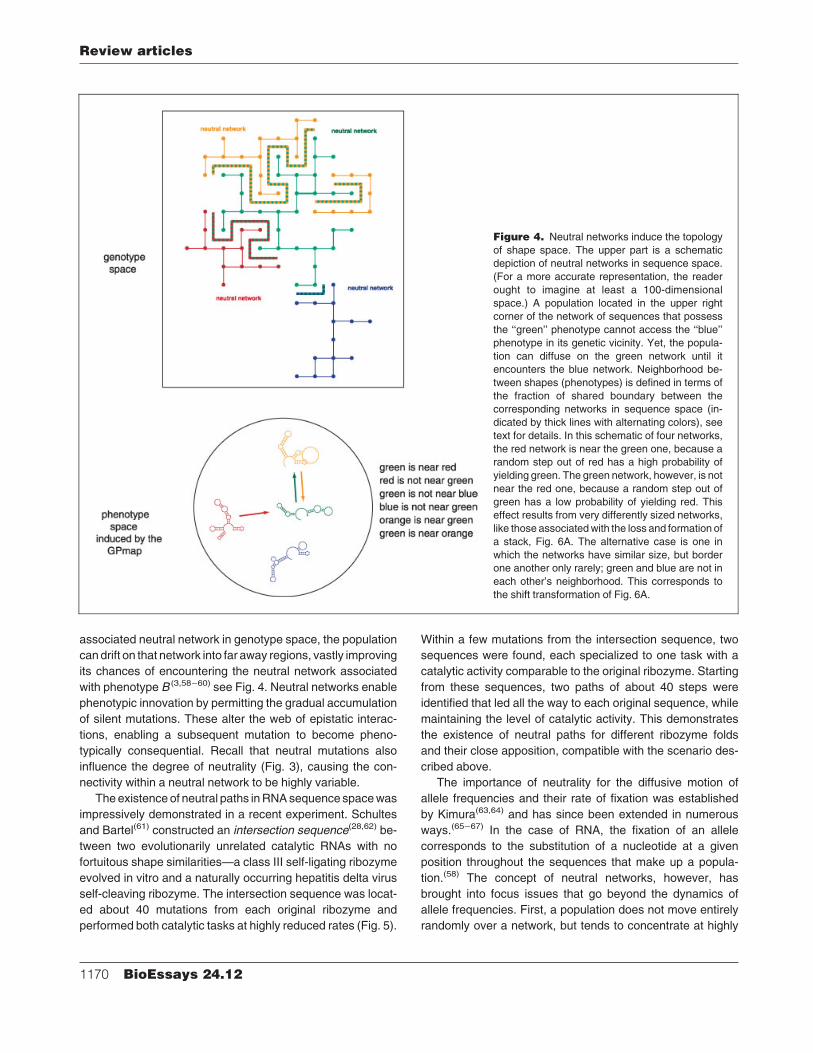
associated neutral network in genotype space, the population

candrift on that network into far away regions, vastly improving

its chances of encountering the neutral network associated

with phenotype B (3,58–60) see Fig. 4. Neutral networks enable

phenotypic innovation by permitting the gradual accumulation

of silent mutations. These alter the web of epistatic interac-

tions, enabling a subsequent mutation to become pheno-

typically consequential. Recall that neutral mutations also

influence the degree of neutrality (Fig. 3), causing the con-

nectivity within a neutral network to be highly variable.

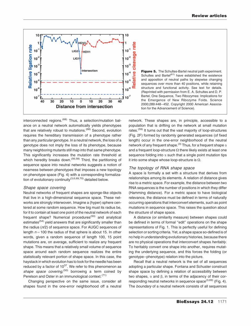
Theexistence of neutral paths inRNAsequence spacewas

impressively demonstrated in a recent experiment. Schultes

and Bartel(61) constructed an intersection sequence(28,62) be-

tween two evolutionarily unrelated catalytic RNAs with no

fortuitous shape similarities—a class III self-ligating ribozyme

evolved in vitro and a naturally occurring hepatitis delta virus

self-cleaving ribozyme. The intersection sequence was locat-

ed about 40 mutations from each original ribozyme and

performed both catalytic tasks at highly reduced rates (Fig. 5).

Within a few mutations from the intersection sequence, two

sequences were found, each specialized to one task with a

catalytic activity comparable to the original ribozyme. Starting

from these sequences, two paths of about 40 steps were

identified that led all the way to each original sequence, while

maintaining the level of catalytic activity. This demonstrates

the existence of neutral paths for different ribozyme folds

and their close apposition, compatible with the scenario des-

cribed above.

The importance of neutrality for the diffusive motion of

allele frequencies and their rate of fixation was established

by Kimura(63,64) and has since been extended in numerous

ways.(65–67) In the case of RNA, the fixation of an allele

corresponds to the substitution of a nucleotide at a given

position throughout the sequences that make up a popula-

tion.(58) The concept of neutral networks, however, has

brought into focus issues that go beyond the dynamics of

allele frequencies. First, a population does not move entirely

randomly over a network, but tends to concentrate at highly

Figure 4. Neutral networks induce the topology

of shape space. The upper part is a schematic

depiction of neutral networks in sequence space.

(For a more accurate representation, the reader

ought to imagine at least a 100-dimensional

space.) A population located in the upper right

corner of the network of sequences that possess

the ‘‘green’’ phenotype cannot access the ‘‘blue’’

phenotype in its genetic vicinity. Yet, the popula-

tion can diffuse on the green network until it

encounters the blue network. Neighborhood be-

tween shapes (phenotypes) is defined in terms of

the fraction of shared boundary between the

corresponding networks in sequence space (in-

dicated by thick lines with alternating colors), see

text for details. In this schematic of four networks,

the red network is near the green one, because a

random step out of red has a high probability of

yielding green. The green network, however, is not

near the red one, because a random step out of

green has a low probability of yielding red. This

effect results from very differently sized networks,

like those associatedwith the loss and formation of

a stack, Fig. 6A. The alternative case is one in

which the networks have similar size, but border

one another only rarely; green and blue are not in

each other’s neighborhood. This corresponds to

the shift transformation of Fig. 6A.

Review articles


interconnected regions.(68) Thus, a selection/mutation bal-

ance on a neutral network automatically yields phenotypes

that are relatively robust to mutations.(68) Second, evolution

requires the hereditary transmission of a phenotype rather

than any particular genotype. In a neutral network, the loss of a

genotype does not imply the loss of its phenotype, because

many neighboringmutants still map into that same phenotype.

This significantly increases the mutation rate threshold at

which heredity breaks down.(56,58) Third, the partitioning of

sequence space into neutral networks suggests a notion of

nearness between phenotypes that imposes a new topology

on phenotype space (Fig. 4) with a corresponding formaliza-

tion of evolutionary continuity(3,6,69,70) detailed below.

Shape space coveringNeutral networks of frequent shapes are sponge-like objects

that live in a high-dimensional sequence space. These net-

works are strongly interwoven. Imagine a (hyper) sphere cen-

tered at some random sequence. How big must its radius be,

for it to contain at least one point of the neutral network of each

frequent shape? Numerical procedures(50) and analytical

estimates(54) yield answers that are significantly smaller than

the radius (n/2) of sequence space. For AUGC sequences of

length n¼ 100 the radius of that sphere is about 15. In other

words, given a random sequence of length 100, 15 point

mutations are, on average, sufficient to realize any frequent

shape. This means that a relatively small volume of sequence

space around each random sequence realizes the entire

statistically relevant portion of shape space. In this case, the

haystack inwhich evolution has to look for the needle has been

reduced by a factor of 1037. We refer to this phenomenon as

shape space covering,(50) borrowing a term coined by

Perelson and Oster in an immunological context.(71)

Changing perspective on the same issue, consider all

shapes found in the one-error neighborhood off a neutral

network. These shapes are, in principle, accessible to a

population that is drifting on the network at small mutation

rates.(59) It turns out that the vast majority of loop-structures

(Fig. 2F) formed by randomly generated sequences (of fixed

length) occur in the one-error neighborhood of the neutral

network of any frequent shape.(3) Thus, for a frequent shape aand a frequent loop-structure O there likely exists at least one

sequence folding into a such that a single point mutation tips

it into some shape whose loop-structure is O.

The topology of RNA shape spaceA space is formally a set with a structure that derives from

relationships among its elements. A relation of distance gives

rise to a metric space. For example, the distance between two

RNA sequences is the number of positions in which they differ

(Hamming distance). For a metric space to have biological

relevance, the distance must be defined in terms of naturally

occurring operations that interconvert elements, such as point

mutations in sequence space. This raises the question about

the structure of shape space.

A distance (or similarity measure) between shapes could

be defined in terms of formal ‘‘edit’’ operations on the shape

representations of Fig. 1. This is perfectly useful for defining

selection or sorting criteria. Yet, a shape space so-defined is of

no help in understanding evolutionary histories, because there

are no physical operations that interconvert shapes heritably.

To heritably convert one shape into another, requires mutat-

ing the underlying sequence, and this forces the folding (or

genotype–phenotype) relation into the picture.

Recall that a neutral network is the set of all sequences

adopting a particular shape. Fontana and Schuster construct

shape space by defining a relation of accessibility between

two shapes, a and b, in terms of the adjacency of their cor-

responding neutral networks in sequence space(3,69) (Fig. 4).

The boundary of a neutral network consists of all sequences

Figure 5. The Schultes-Bartel neutral path experiment.

Schultes and Bartel(61) have established the existence

and apposition of neutral paths by stepwise changing

sequences over more than 40 positions, while retaining

structure and functional activity. See text for details.

(Reprinted with permission from E. A. Schultes and D. P.

Bartel, One Sequence, Two Ribozymes: Implications for

the Emergence of New Ribozyme Folds. Science

2000;289:448–452. Copyright 2000 American Associa-

tion for the Advancement of Science).

Review articles


that are one mutation off the network. The intersection of the

neutral network of bwith the boundary of the neutral network ofa, relative to the total boundary of a’s network, is a measure of

the probability that one step off a random point on the neutral

network of a there is a sequence folding into b. Accessibility,however, is not symmetric and thereforenot adistance (Fig. 4).

To wit: the loss and formation of a stack. A stack in shape awillbe only marginally stable in most sequences realizing a. As a

consequence, pointmutations aremore likely to cause its loss.

In contrast, creating a stack in a single mutation requires

specially poised sequences. RNA folding is a simple mechan-

ism giving rise to strongly asymmetric transition probabilities.

A shape bmay be significantly easier to access from shape athan the other way around.

To convert accessibility distributions into a binary attribute

of nearness, we define the neighborhood of shape a as the setcontaining a and all shapes accessible from a above a certain

likelihood(3,69)—a ‘‘frequent neighbor’’ akin to the notion of a

frequent shape. The major implications of this construction do

not depend on the exact value of the cutoff point.(6) Because

accessibility is asymmetric, shape bmay be near (read: in the

neighborhood of) a, but amay not be near b. This constructionof shape-neighborhood is technically consistent with the

formalization of the neighborhood concept in topology.(6,72)

Phenotype space has thus been organized into neighbor-

hoods without assuming a distance. To non-topologists, this

may seem counterintuitive, since common sense conceives

neighborhood in terms of ‘‘small distance’’.

The notion of neighborhood is sufficient to define continuity

mathematically. In the present context, a genetic path is con-

tinuous, if the offspring of a sequence is near that sequence

in the topology of genotype space. Specifically, offspring

and parent differ by one point mutation. Similarly, a path in

phenotype space is continuous if the phenotype of the off-

spring is near the phenotype of the parent in the accessibility

topology just defined. Think of an evolutionary trajectory as a

time series of genotypes (G) with their associated phenotypes

(P)—a GP path. A GP path is continuous, if it is continuous

at the genetic and the associated phenotypic level. The key

question now becomes: given any two shapes, is there a con-

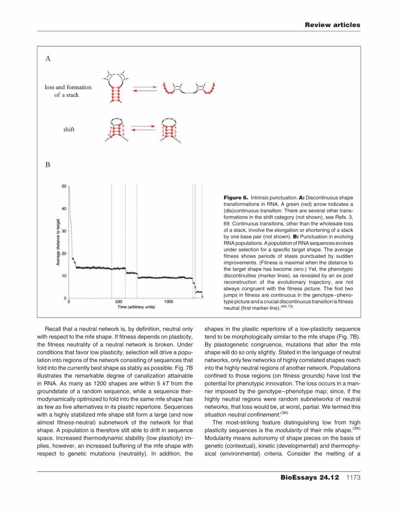
tinuous GP path connecting them? The answer is no. There is

a well-defined class of shape transformations (Fig. 6A) that is

discontinuous along any continuous genetic path.(3) A transi-

tion from one neutral network to another involving such a

shape transformation, while possible by a single point muta-

tion, depends on very special, hence relatively rare, sequ-

ences. The two classes of discontinuous transformations

are stack formations and shifts (Fig. 6A). They both require

the simultaneous change of several base pairs, since par-

tial rearrangements result in thermodynamically unstable

intermediates. The notion of discontinuity reflects precisely

those transformations that are difficult to achieve by virtue of

the mechanisms underlying the map from genotype to

phenotype. This is the RNA analogue of ‘‘developmental

constraints’’.

A fewobservations deserveemphasis. First, (dis)continuity

cross-cuts morphological (dis)similarity. Some transitions be-

tween similar shapes are discontinuous (e.g. the shift in

Fig. 6A) and some transitions between dissimilar shapes are

continuous (e.g. the loss of a stack). Second, the notion of

discontinuity defined here is not related to sudden jumps in

fitnessor thediscreteness in thevariationofa trait. Theclasses

of discontinuity are caused by the genotype–phenotype map

and thus remain the same regardless of the further mapping

from phenotypes to fitness. (Of course, the particular shapes

observed at discontinuous transitions will depend on the

fitness map.) Third, the dynamical signature of this phenotype

topology ispunctuation (Fig. 6B).Apopulationof replicating and

mutating sequences under selection drifts on the neutral net-

work of the currently best shape until it encounters a gateway to

a network that conveys some advantage or is fitness-neutral.

That encounter, however, is evidently not under the control of

selection. While similar to the phenomenon of punctuated

equilibrium recognized by Eldredge and Gould(74) in the fossil

record of species evolution, punctuation in evolving RNA popu-

lations occurs in the absence of externalities (such asmeteorite

impact or abrupt climate change in the species case). We refer

to it as intrinsic punctuation since it reflects the variational

properties of the underlying developmental architecture.

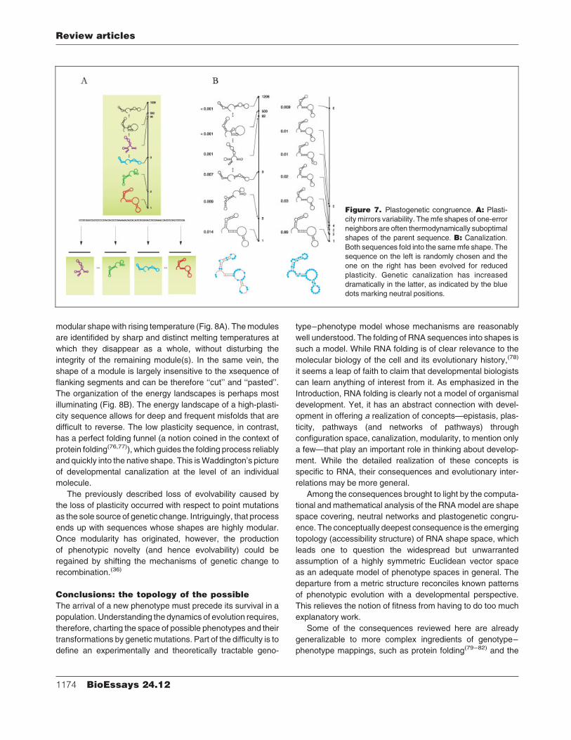
Plastogenetic congruence,canalization and modularityThe RNA folding map exhibits a consequential correlation

between plasticity and variability. The mfe shapes realized

in the one-error neighborhood of a sequence are, with high

frequency, a subset of the shapes in the plastic repertoire

of that sequence(36) (Fig. 7A). A point mutation oftentimes

stabilizes a shape that is suboptimal in the parent, promoting

it to mfe shape in the mutant. We termed this correlation

plastogenetic congruence(36) to emphasize that plasticity and

(genetic) variability are correlated, because both depend on

the same structure-forming mechanisms. The significance

of such congruence consists in directly coupling a change

in plasticity to a change in genetic variability. While genetic

variability is a property affecting the future evolution of a

lineage, plasticity affects an individual in the present and can

be an easy target of selection. Since plasticity correlates with

the shape of things to come, selection on plasticity has a direct

impact on a future capacity. In RNA, environmental canaliza-

tion (the reduction of plasticity by tightening the genetic deter-

mination of the mfe shape) entails genetic canalization (the

curtailing of phenotypic novelty accessible by mutation). This

was hypothesized by Wagner et al.(75) on the basis of popula-

tion genetic models. Selection pressures favoring the reduc-

tion of plasticity may arise from the fitness costs associated

with plasticity.(37)

Review articles


Recall that a neutral network is, by definition, neutral only

with respect to the mfe shape. If fitness depends on plasticity,

the fitness neutrality of a neutral network is broken. Under

conditions that favor low plasticity, selection will drive a popu-

lation into regions of the network consisting of sequences that

fold into the currently best shape as stably as possible. Fig. 7B

illustrates the remarkable degree of canalization attainable

in RNA. As many as 1200 shapes are within 5 kT from the

groundstate of a random sequence, while a sequence ther-

modynamically optimized to fold into the samemfe shape has

as few as five alternatives in its plastic repertoire. Sequences

with a highly stabilized mfe shape still form a large (and now

almost fitness-neutral) subnetwork of the network for that

shape. A population is therefore still able to drift in sequence

space. Increased thermodynamic stability (low plasticity) im-

plies, however, an increased buffering of the mfe shape with

respect to genetic mutations (neutrality). In addition, the

shapes in the plastic repertoire of a low-plasticity sequence

tend to be morphologically similar to the mfe shape (Fig. 7B).

By plastogenetic congruence, mutations that alter the mfe

shape will do so only slightly. Stated in the language of neutral

networks, only few networks of highly correlated shapes reach

into the highly neutral regions of another network. Populations

confined to those regions (on fitness grounds) have lost the

potential for phenotypic innovation. The loss occurs in a man-

ner imposed by the genotype–phenotype map; since, if the

highly neutral regions were random subnetworks of neutral

networks, that loss would be, at worst, partial. We termed this

situation neutral confinement.(36)

The most-striking feature distinguishing low from high

plasticity sequences is the modularity of their mfe shape.(36)

Modularity means autonomy of shape pieces on the basis of

genetic (contextual), kinetic (developmental) and thermophy-

sical (environmental) criteria. Consider the melting of a

Figure 6. Intrinsic punctuation.A:Discontinuous shapetransformations in RNA. A green (red) arrow indicates a

(dis)continuous transition. There are several other trans-

formations in the shift category (not shown), see Refs. 3,

69. Continuous transitions, other than the wholesale loss

of a stack, involve the elongation or shortening of a stack

by one base pair (not shown). B: Punctuation in evolving

RNApopulations.ApopulationofRNAsequencesevolves

under selection for a specific target shape. The average

fitness shows periods of stasis punctuated by sudden

improvements. (Fitness is maximal when the distance to

the target shape has become zero.) Yet, the phenotypic

discontinuities (marker lines), as revealed by an ex post

reconstruction of the evolutionary trajectory, are not

always congruent with the fitness picture. The first two

jumps in fitness are continuous in the genotype–pheno-

typepicture andacrucial discontinuous transition is fitness

neutral (first marker line).(69,73)

Review articles


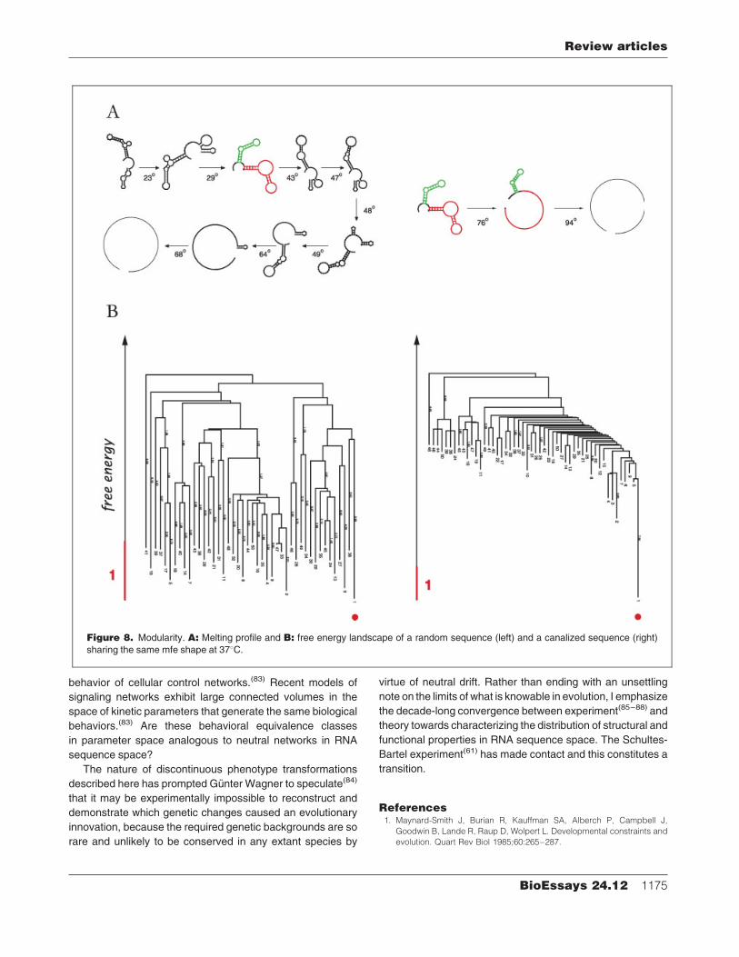
modular shapewith rising temperature (Fig. 8A). Themodules

are identifided by sharp and distinct melting temperatures at

which they disappear as a whole, without disturbing the

integrity of the remaining module(s). In the same vein, the

shape of a module is largely insensitive to the xsequence of

flanking segments and can be therefore ‘‘cut’’ and ‘‘pasted’’.

The organization of the energy landscapes is perhaps most

illuminating (Fig. 8B). The energy landscape of a high-plasti-

city sequence allows for deep and frequent misfolds that are

difficult to reverse. The low plasticity sequence, in contrast,

has a perfect folding funnel (a notion coined in the context of

protein folding(76,77)), which guides the folding process reliably

and quickly into the native shape. This isWaddington’s picture

of developmental canalization at the level of an individual

molecule.

The previously described loss of evolvability caused by

the loss of plasticity occurred with respect to point mutations

as the sole source of genetic change. Intriguingly, that process

ends up with sequences whose shapes are highly modular.

Once modularity has originated, however, the production

of phenotypic novelty (and hence evolvability) could be

regained by shifting the mechanisms of genetic change to

recombination.(36)

Conclusions: the topology of the possible

The arrival of a new phenotype must precede its survival in a

population. Understanding the dynamics of evolution requires,

therefore, charting the space of possible phenotypes and their

transformations by genetic mutations. Part of the difficulty is to

define an experimentally and theoretically tractable geno-

type–phenotype model whose mechanisms are reasonably

well understood. The folding of RNA sequences into shapes is

such a model. While RNA folding is of clear relevance to the

molecular biology of the cell and its evolutionary history,(78)

it seems a leap of faith to claim that developmental biologists

can learn anything of interest from it. As emphasized in the

Introduction, RNA folding is clearly not a model of organismal

development. Yet, it has an abstract connection with devel-

opment in offering a realization of concepts—epistasis, plas-

ticity, pathways (and networks of pathways) through

configuration space, canalization, modularity, to mention only

a few—that play an important role in thinking about develop-

ment. While the detailed realization of these concepts is

specific to RNA, their consequences and evolutionary inter-

relations may be more general.

Among the consequences brought to light by the computa-

tional and mathematical analysis of the RNAmodel are shape

space covering, neutral networks and plastogenetic congru-

ence. The conceptually deepest consequence is the emerging

topology (accessibility structure) of RNA shape space, which

leads one to question the widespread but unwarranted

assumption of a highly symmetric Euclidean vector space

as an adequate model of phenotype spaces in general. The

departure from a metric structure reconciles known patterns

of phenotypic evolution with a developmental perspective.

This relieves the notion of fitness from having to do too much

explanatory work.

Some of the consequences reviewed here are already

generalizable to more complex ingredients of genotype–

phenotype mappings, such as protein folding(79–82) and the

Figure 7. Plastogenetic congruence. A: Plasti-city mirrors variability. Themfe shapes of one-error

neighbors are often thermodynamically suboptimal

shapes of the parent sequence. B: Canalization.Both sequences fold into the samemfe shape. The

sequence on the left is randomly chosen and the

one on the right has been evolved for reduced

plasticity. Genetic canalization has increased

dramatically in the latter, as indicated by the blue

dots marking neutral positions.

Review articles


behavior of cellular control networks.(83) Recent models of

signaling networks exhibit large connected volumes in the

space of kinetic parameters that generate the same biological

behaviors.(83) Are these behavioral equivalence classes

in parameter space analogous to neutral networks in RNA

sequence space?

The nature of discontinuous phenotype transformations

described here has prompted Gunter Wagner to speculate(84)

that it may be experimentally impossible to reconstruct and

demonstrate which genetic changes caused an evolutionary

innovation, because the required genetic backgrounds are so

rare and unlikely to be conserved in any extant species by

virtue of neutral drift. Rather than ending with an unsettling

note on the limits of what is knowable in evolution, I emphasize

the decade-long convergence between experiment(85–88) and

theory towards characterizing the distribution of structural and

functional properties in RNA sequence space. The Schultes-

Bartel experiment(61) has made contact and this constitutes a

transition.

References1. Maynard-Smith J, Burian R, Kauffman SA, Alberch P, Campbell J,

Goodwin B, Lande R, Raup D, Wolpert L. Developmental constraints and

evolution. Quart Rev Biol 1985;60:265–287.

Figure 8. Modularity. A: Melting profile and B: free energy landscape of a random sequence (left) and a canalized sequence (right)

sharing the same mfe shape at 378C.

Review articles


2. Gould SJ. The Structure of Evolutionary Theory. Cambridge, MA:

Belknap/Harvard University Press; 2002.

3. Fontana W, Schuster P. Continuity in evolution: On the nature of transi-

tions. Science 1998;280:1451–1455.

4. Carroll SB, Grenier JK, Weatherbee SD. From DNA to diversity. Malden,

Massachusetts: Blackwell Science; 2001.

5. Wilkins AS. The evolution of developmental pathways. Sunderland,

Massachusetts: Sinauer Associates, Inc; 2002.

6. Stadler BMR, Stadler PF, Wagner G, Fontana W. The topology of the

possible: Formal spaces underlying patterns of evolutionary change.

J Theor Biol 2001;213:241–274.

7. Zuker M, Sankoff D. RNA secondary structures and their prediction. Bull.

Math. Biol 1984;46:591–621.

8. Turner DH, Sugimoto N, Freier S. RNA structure prediction. Ann Rev

Biophys Biophys Chem 1988;17:167–192.

9. Wuchty S, Fontana W, Hofacker IL, Schuster P. Complete suboptimal

folding of RNA and the stability of secondary structures. Biopolymers

1999;49:145–165.

10. Jaeger JA, Turner DH, Zuker M. Improved predictions of secon-

dary structures for RNA. Proc Natl Acad Sci USA 1989;86:7706–

7710.

11. He L, Kierzek R, SantaLucia J, Walter AE, Turner DH. Nearest-neighbour

parameters for G-U mismatches. Biochemistry 1991;30:11124.

12. Walter AE, Turner DH, Kim J, Lyttle MH, Muller P, Mathews DH, Zuker M.

Coaxial stacking of helices enhances binding of oligoribonucleotides

and improves prediction of RNA folding. Proc Natl Acad Sci 1994;91:

9218–9222.

13. Mathews DH, Sabina J, Zuker M, Turner DH. Expanded sequence

dependence of thermodynamic parameters improves prediction of RNA

secondary structure. J Mol Biol 1999;288:911–940.

14. Waterman MS, Smith TF. RNA secondary structure: A complete

mathematical analysis. Mathematical Biosciences 1978;42:257–266.

15. Nussinov R, Jacobson AB. Fast algorithm for predicting the secondary

structure of single-stranded RNA. Proc Natl Acad Sci USA 1980;77:

6309–6313.

16. Zuker M, Stiegler P. Optimal computer folding of larger RNA sequences

using thermodynamics and auxiliary information. Nucleic Acids Res

1981;9:133–148.

17. Bellman RE. Dynamic Programming. Princeton, NJ: Princeton University

Press; 1957.

18. Rivas E, Eddy SR. A dynamic programming algorithm for RNA

structure prediction including pseudoknots. J Mol Biol 1999;285:2053–

2068.

19. Isambert H, Siggia ED. Modeling RNA folding paths with pseudoknots:

Application to hepatitis delta virus ribozyme. Proc Natl Acad Sci USA

2000;97:6515–6520.

20. Banerjee AR, Jaeger JA, Turner DH. Thermal unfolding of a group I

ribozyme: The low-temperature transition is primarily disruption of tertiary

structure. Biochemistry 1993;32:153–163.

21. Gutell RR. Evolutionary chracteristics of RNA: Inferring higher order

structure from patterns of sequence variation. Curr Opin Struct Biol 1993;

3:313–322.

22. Hofacker IL, Fontana W, Stadler PF, Bonhoeffer S, Tacker M, Schuster P.

Fast folding and comparison of RNA secondary structures. Mh. Chem

1994;125:167–188.

23. Waterman MS. Introduction to Computational Biology: Sequences, Maps

and Genomes. London: Chapman & Hall; 1995.

24. Higgs P. RNA secondary structure: physical and computational aspects.

Quart Rev Biophys 2000;33:199–253.

25. Mironov A, Lebedev VF. A kinetic model of RNA folding. BioSystems

1993;30:49–56.

26. Gultyaev AP, van Batenburg FHD, Pleij CWA. The computer simulation of

RNA folding pathways using a genetic algorithm. J Mol Biol 1995;250:

37–41.

27. Morgan SR, Higgs PG. Evidence for kinetic effects in the folding of large

RNA molecules. J Chem Phys 1996;105:7152–7157.

28. Flamm C, Fontana W, Hofacker IL, Schuster P. RNA folding at elementary

step resolution. RNA 2000;6:325–338.

29. Biebricher CK, Luce R. In vitro recombination and terminal elongation of

RNA by Qb replicase. EMBO J 1992;11:5129–5135.

30. Flamm C, Hofacker IL, Maurer-Stroh S, Stadler PF, Zehl M. Design of

multistable RNA molecules. RNA 2001;7:254–265.

31. Jacob C, Breton N, Daegelen P. Stochastic theories of the activated

complex and the activated collision:The RNA example. J Chem Phys

1997;107:2903–2912.

32. Waddington CH. The Strategy of the Genes. New York, NY: MacMillan

Co; 1957.

33. Griesemer J. The units of evolutionary transition. Selection 2000;1:67–70.

34. McCaskill JS. The equilibrium partition function and base pair binding

probabilities for RNA secondary structure. Biopolymers 1990;29:1105–

1119.

35. Huynen M, Gutell R, Konings D. Assessing the reliability of RNA folding

using statistical mechanics. J Mol Biol 1997;267:1104–1112.

36. Ancel L, Fontana W. Plasticity, evolvability and modularity in RNA. J of

Exp. Zoology (Molecular and Developmental Evolution) 2000;288:242–

283.

37. Scheiner SM. Genetics and evolution of phenotypic plasticity. Annu Rev

Ecol Syst 1993;24:35–38.

38. Wagner GP, Laubichler MD, Bagheri-Chaichian H. Genetic measure-

ment theory of epistatic effects. Genetica 1998;102(103):569–580.

39. Wagner GP, Altenberg L. Complex adaptations and the evolution of

evolvability. Evolution 1996;50:967–976.

40. Wagner A. Does evolutionary plasticity evolve? Evolution 1996;50:1008–

1023.

41. Waddington CH. Canalization of development and the inheritance of

acquired characters. Nature 1942;3811:563–565.

42. Wilkins AS. Genetic analysis of animal development. New York, NY: John

Wiley and Sons; 1986.

43. Scharloo W. Canalization: Genetic and developmental aspects. Annu

Rev Ecol Syst 1991;22:65–73.

44. Csete ME, Doyle JC. Reverse engineering of biological complexity.

Nature 2002;295:1664–1669.

45. Fontana W, Schuster P. A Computer Model of Evolutionary Optimization.

Biophys Chem 1987;26:123–147.

46. Fontana W, Stadler PF, Bornberg-Bauer EG, Griesmacher T, Hofacker IL,

Tacker M, Tarazona P, Weinberger ED, Schuster P. RNA folding and

combinatory landscapes. Phys Rev E 1993;47:2083–2099.

47. Fontana W, Konings DAM, Stadler PF, Schuster P. Statistics of RNA

secondary structures. Biopolymers 1993;33:1389–1404.

48. Tacker M, Stadler PF, Bornberg-Bauer EG, Hofacker IL, Schuster P.

Algorithm independent properties of RNA secondary structure predic-

tions. Eur Biophys J 1996;25:115–130.

49. Schultes E, Hraber PT, LaBean T. Estimating the contributions of

selection and self-organisation in RNA secondary structure. J Mol Evol

1999;49:76–83.

50. Schuster P, Fontana W, Stadler PF, Hofacker I. From sequences to

shapes and back: A case study in RNA secondary structures. Proc Roy

Soc. (London)B 1994;255:279–284.

51. Hofacker IL, Schuster P, Stadler PF. Combinatorics of RNA secondary

structures. Discr Appl Math 1999;89:177–207.

52. Gruner W, Giegerich R, Strothmann D, Reidys C, Weber J, Hofacker IL,

Stadler PF, Schuster P. Analysis of RNA sequence structure maps by

exhaustive enumeration. I. Neutral networks. Mh Chem 1996;127:355–

374.

53. Haslinger C, Stadler PF. RNA structures with pseudo-knots. Bull Math

Biol 1999;61:437–467.

54. Gruner W, Giegerich R, Strothmann D, Reidys C, Weber J, Hofacker IL,

Stadler PF, Schuster P. Analysis of RNA sequence structure maps by

exhaustive enumeration. II. Structure of neutral networks and shape

space covering. Mh Chem 1996;127:375–389.

55. Schuster P. Landscapes and molecular evolution. Physica D 1997;107:

351–365.

56. Reidys C, Stadler PF, Schuster P. Generic properties of combinatory

maps. Neutral networks of RNA secondary structures. Bull Math Biol

1997;59:339–397.

57. Wright S. Evolution in mendelian populations. Genetics 1931;16:97–

159.

58. Huynen MA, Stadler P, Fontana W. Smoothness within ruggedness: The

role of neutrality in adaptation. Proc Natl Acad Sci USA 1996;93:397–

401.

Review articles


59. Huynen MA. Exploring phenotype space through neutral evolution. J Mol

Evol 1996;43:165–169.

60. van Nimwegen E, Crutchfield JP. Metastable evolutionary dynamics:

Crossing fitness barriers or escaping via neutral paths? Bull Math Biol

2000;62:799–848.

61. Schultes EA, Bartel DP. One sequence, two ribozymes: Implications

for the emergence of new ribozyme folds. Science 2000;289:448–452.

62. Reidys C, Stadler PF. Bio-molecular shapes and algebraic structures.

Computers Chem 1996;20:85–94.

63. Kimura M. Evolutionary rate at the molecular level. Nature 1968;217:624–

626.

64. Kimura M. The Neutral Theory of Molecular Evolution. Cambridge, UK:

Cambridge University Press; 1983.

65. Derrida B, Peliti L. Evolution in a flat fitness landscape. Bull Math Biol

1991;53:355–382.

66. Gavrilets S. Evolution and speciation on holey adaptive landscapes.

Trends Ecol Evol 1997;12:307–312.

67. Newman MEJ, Engelhardt R. Effects of selective neutrality on the evolu-

tion of molecular species. Proc Roy Soc (London)B 1998;265:1333–1338.

68. van Nimwegen E, Crutchfield JP, Huynen M. Neutral evolution of

mutational robustness. Proc Natl Acad Sci USA 1999;96:9716–9720.

69. Fontana W, Schuster P. Shaping space: The possible and the attainable

in RNA genotype-phenotype mapping. J Theor Biol 1998;194:491–515.

70. Cupal J, Kopp S, Stadler PF. RNA shape space topology. Artificial Life

2000;6:3.

71. Perelson AS, Oster GF. Theoretical studies on clonal selection: minimal

antibody repertoire size and reliability of self-non-self discrimination.

J Theor Biol 1979;81:645–670.

72. Gaal SA. Point Set Topology. New York: Academic Press; 1964.

73. Schuster P, Fontana W. Chance and necessity in evolution: Lessons from

RNA. Physica D 1999;133:427–452.

74. Eldredge N, Gould SJ. Punctuated equilibria: an alternative to phyletic

gradualism. In: Schopf TJM, editor. Models in Paleobiology San

Francisco CA: Freeman: Cooper & Co; 1972;82–115.

75. Wagner GP, Booth G, Bagheri-Chaichian H. A population genetic theory

of canalization. Evolution 1997;51:329–347.

76. Leopold PE, Montal M, Onuchic JN. Protein folding funnels -a kinetic

approach to the sequence structure relationship. Proc Natl Acad Sci

USA 1992;89:8721–8725.

77. Dill KA, Chan HS. From Levinthal to pathways to funnels. Nature Struct

Biol 1997;4:10–19.

78. Gilbert W. The RNA world. Nature 1986;319:618.

79. Vendruscolo M, Maritan A, Banavar JR. Stability threshold as a

selection principle for protein design. Phys Rev Lett 1997;78:3967–

3970.

80. Bussemaker HJ, Thirumalai D, Bhattacharjee JK. Thermodynamic

stability of folded proteins against mutations. Phys Rev Lett 1997;79:

3530–3533.

81. Bornberg-Bauer E, Chan HS. Modeling evolutionary landscapes: Muta-

tional stability, topology, and superfunnels in sequence space. Proc Natl

Acad Sci USA 1999;96:10689–10694.

82. Buchler NEG, Goldstein RA. Surveying determinants of protein structure

designability across different energy models and amino-acid alphabets:

A consensus. J Chem Phys 2000;112:2533–2547.

83. von Dassow G, Meir E, Munro E, Odell GM. The segment polarity

network is a robust developmental module. Nature 2000;406:188–

192.

84. Wagner GP. What is the promise of developmental evolution? Part II:

A causal explanation of evolutionary innovations may be impossible.

J Exp Zool (Mol Dev Evol) 2001;291:305–309.

85. Spiegelman S. An approach to experimental analysis of precellular

evolution. Quart Rev Biophys 1971;4:213–253.

86. Ellington AD, Szostak JW. In vitro selection of RNA molecules that bind

specific ligands. Nature 1990;346:818–822.

87. Bartel DP, Szostak JW. Isolation of new ribozymes from a large pool of

random sequences. Science 1993;261:1411–1418.

88. Wright MC, Joyce GF. Continuous in vitro evolution of catalytic function.

Science 1997;276: 614–617.

Review articles


modelling ‘evo-devo’ with rna

Documents