modelling dependence in ﬁnance using...

Modelling dependence in finance

using copulas∗

Statistics 2001, Concordia University, Montreal†

Thierry Roncalli

Groupe de Recherche OperationnelleCredit Lyonnais

∗These slides may be downloaded from http://gro.creditlyonnais.fr (the direct linkis http://gro.creditlyonnais.fr/content/wp/copula-stat2001-canada.pdf).†I would like to thank Professor Christian Genest for his invitation.

Agenda

1. The Gaussian assumption in finance

2. Copulas and multivariate financial models

3. An open field for risk management

• Market risk

• Operational risk

• Credit risk

4. New pricing methods with copulas

• Multi-asset options

• Credit derivatives

Modelling dependence in finance using copulas 1

1 The Gaussian assumption in finance

We consider the ‘universal’ financial model. Let (Ω,F ,P) be theprobability space. The asset prices processes S1 (t) and S2 (t) aregiven by the SDE representation

dS1 (t) = µ1S1 (t) dt + σ1S1 (t) dW1 (t)dS2 (t) = µ2S2 (t) dt + σ2S2 (t) dW2 (t)

where W1 (t) and W2 (t) are two Ft–brownian motions with

E[

W1 (t)W2 (t) | Ft0

]

= ρ (t− t0)

It comes that the logarithm return of assets is gaussian (= Gaussianassumption in finance).

Empirical facts: Asset returns are not gaussian (see the financialeconometric literature on ARCH, long-memory, Levy processes, etc.).

Problem: Univariate financial models are not gaussian, butmultivariate financial models are gaussian!

Modelling dependence in finance using copulasThe Gaussian assumption in finance 1-1

2 Copulas and multivariate financial models1. How to define multivariate financial models compatible with

univariate non-Gaussian financial models?

Copula = a powerful tool

2. How to obtain tractable multivariate financial models (in terms ofcomputational time)?

3. How to specify multivariate financial models which may beunderstood/used by the finance industry?

Copula = a promising tool

Copulas have been already incorporated in some software solutions:

• SAS Risk Dimensions

• Palisade @Risk

Modelling dependence in finance using copulasCopulas and multivariate financial models 2-1

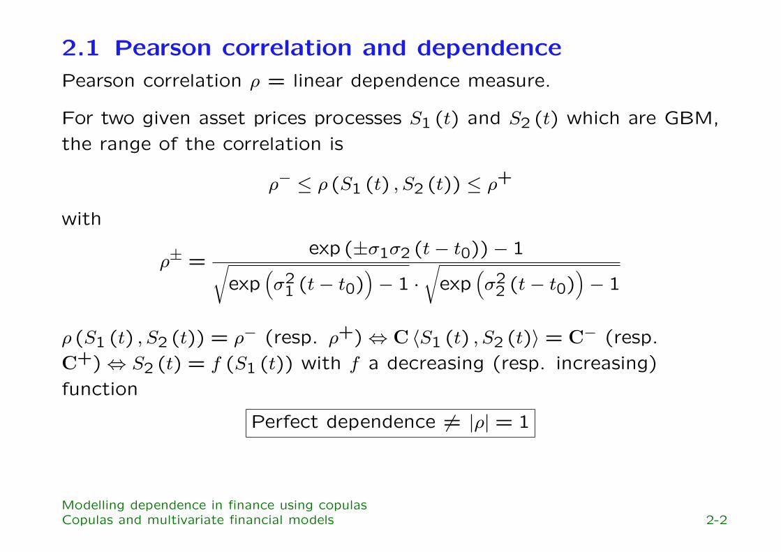
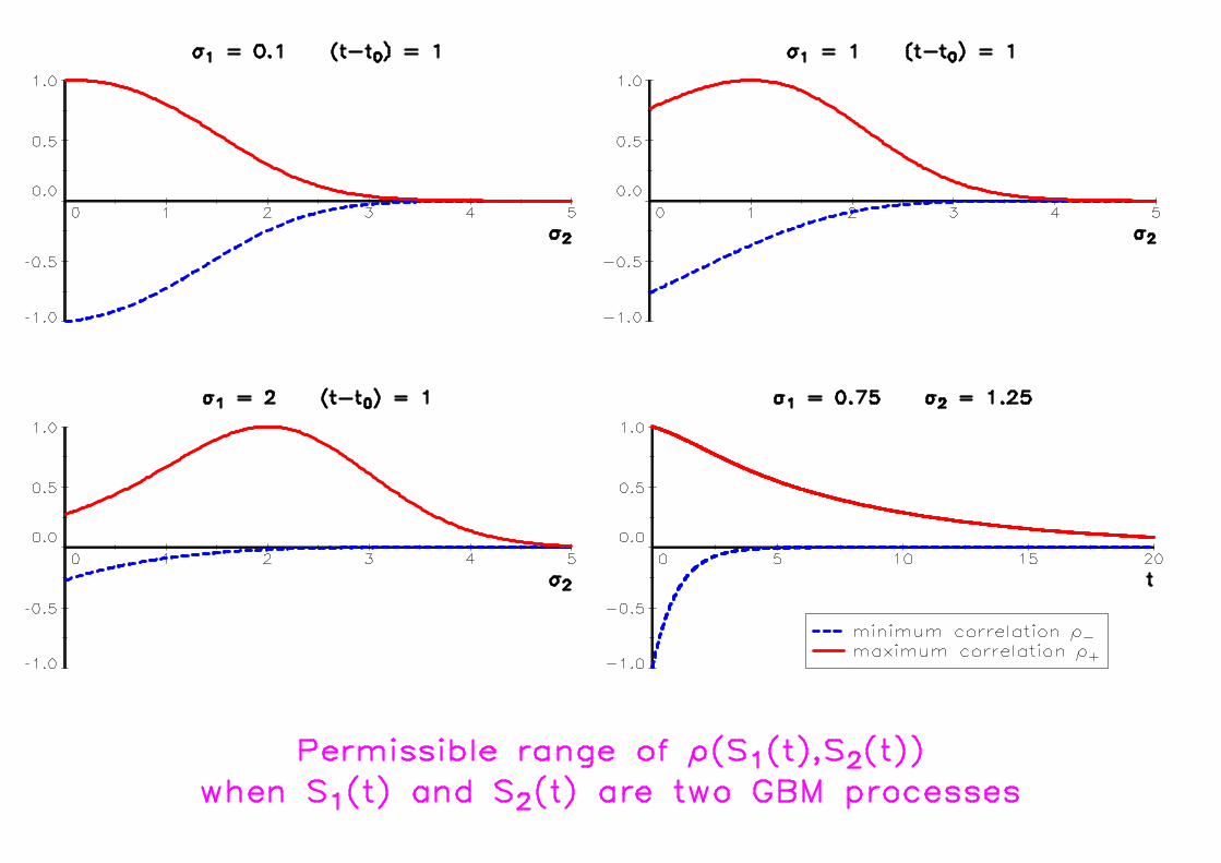
2.1 Pearson correlation and dependencePearson correlation ρ = linear dependence measure.

For two given asset prices processes S1 (t) and S2 (t) which are GBM,the range of the correlation is

ρ− ≤ ρ (S1 (t) , S2 (t)) ≤ ρ+

with

ρ± =exp (±σ1σ2 (t− t0))− 1

√

exp(

σ21 (t− t0)

)

− 1 ·√

exp(

σ22 (t− t0)

)

− 1

ρ (S1 (t) , S2 (t)) = ρ− (resp. ρ+) ⇔ C 〈S1 (t) , S2 (t)〉 = C− (resp.C+) ⇔ S2 (t) = f (S1 (t)) with f a decreasing (resp. increasing)function

Perfect dependence 6= |ρ| = 1


2.2 Copula: a new tool in finance

• introduced by Embrechts et al. [14].

• Market risk: Bouye et al. [2], Cherubini et al. [8], Durrleman etal. [13], Embrechts et al. [15], Luciano et al. [24], Tibiletti [33].

• Credit risk: Coutant et al. [11], Frey et al. [17], Georges et al.[18], Giesecke [19], Hamilton et al. [20], Lindskog et al. [23],Maccarinelli et al. [25].

• Operational risk: Ceske et al. [5] [6], Frachot et al. [16].

• Asset prices modelling: Bouye et al. [4], Malavergne et al. [26],Patton [27], Rockinger et al. [28], Scaillet [31].

• Credit derivatives pricing: Li [21], Georges et al. [18],Schonbucher et al. [32].

• Multi-asset options pricing: Bikos [1], Cherubini et al. [7],Coutant et al. [10], Durrleman [12], Rosenberg [29] [30].


2.3 Copulas in a nutshell

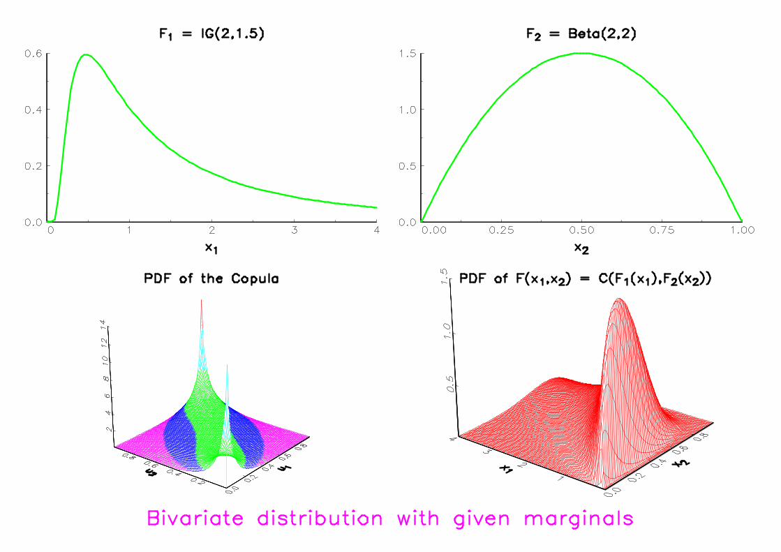
A copula function C is a multivariate probability distribution withuniform [0,1] margins.

C (F1 (x1) , . . . ,FN (xN)) defines a multivariate cdf F with marginsF1, . . . ,FN ⇒ F is a probability distribution with given marginals.

The copula function of the random variables (X1, . . . , XN) isinvariant under strictly increasing transformations (∂xhn (x) > 0):

C 〈X1, . . . , XN〉 = C 〈h1 (X1) , . . . , hN (XN)〉

... the copula is invariant while the margins may be changed at will,it follows that is precisely the copula which captures those propertiesof the joint distribution which are invariant under a.s. stricklyincreasing transformations (Schweizer and Wolff [1981]).

⇒ Copula = dependence function of r.v. (Deheuvels [1978]).


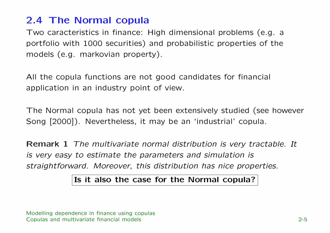
2.4 The Normal copulaTwo caracteristics in finance: High dimensional problems (e.g. aportfolio with 1000 securities) and probabilistic properties of themodels (e.g. markovian property).

All the copula functions are not good candidates for financialapplication in an industry point of view.

The Normal copula has not yet been extensively studied (see howeverSong [2000]). Nevertheless, it may be an ‘industrial’ copula.

Remark 1 The multivariate normal distribution is very tractable. Itis very easy to estimate the parameters and simulation isstraightforward. Moreover, this distribution has nice properties.

Is it also the case for the Normal copula?


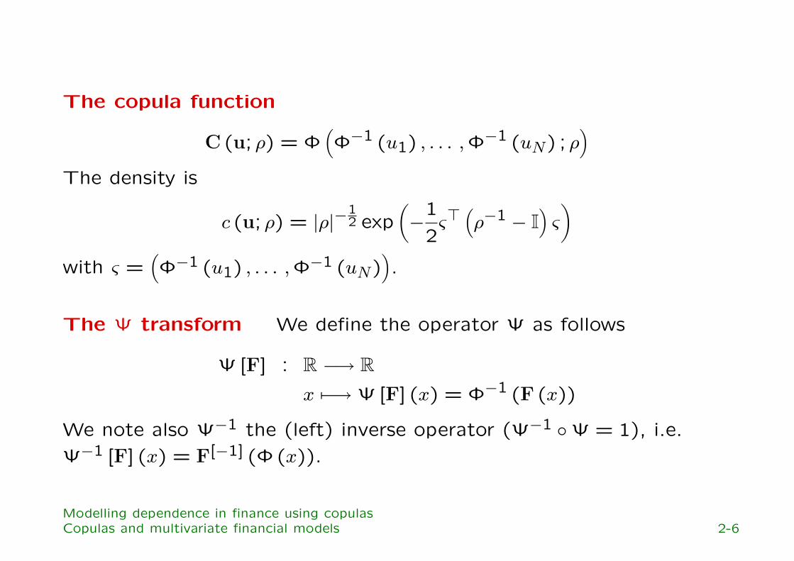
The copula function

C (u; ρ) = Φ(

Φ−1 (u1) , . . . ,Φ−1 (uN) ; ρ)

The density is

c (u; ρ) = |ρ|−12 exp

(

−12

ς>(

ρ−1 − I)

ς)

with ς =(

Φ−1 (u1) , . . . ,Φ−1 (uN))

.

The Ψ transform We define the operator Ψ as follows

Ψ [F] : R −→ Rx 7−→ Ψ[F] (x) = Φ−1 (F (x))

We note also Ψ−1 the (left) inverse operator (Ψ−1 Ψ = 1), i.e.Ψ−1 [F] (x) = F[−1] (Φ (x)).


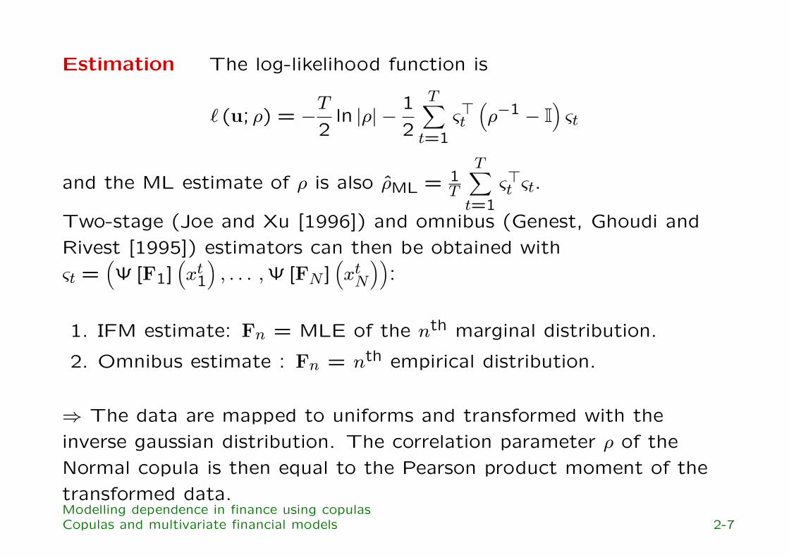
Estimation The log-likelihood function is

` (u; ρ) = −T2

ln |ρ| −12

T∑

t=1ς>t

(

ρ−1 − I)

ςt

and the ML estimate of ρ is also ρML = 1T

T∑

t=1ς>t ςt.

Two-stage (Joe and Xu [1996]) and omnibus (Genest, Ghoudi andRivest [1995]) estimators can then be obtained withςt =

(

Ψ[F1](

xt1

)

, . . . ,Ψ[FN ](

xtN

))

:

1. IFM estimate: Fn = MLE of the nth marginal distribution.

2. Omnibus estimate : Fn = nth empirical distribution.

⇒ The data are mapped to uniforms and transformed with theinverse gaussian distribution. The correlation parameter ρ of theNormal copula is then equal to the Pearson product moment of thetransformed data.Modelling dependence in finance using copulasCopulas and multivariate financial models 2-7

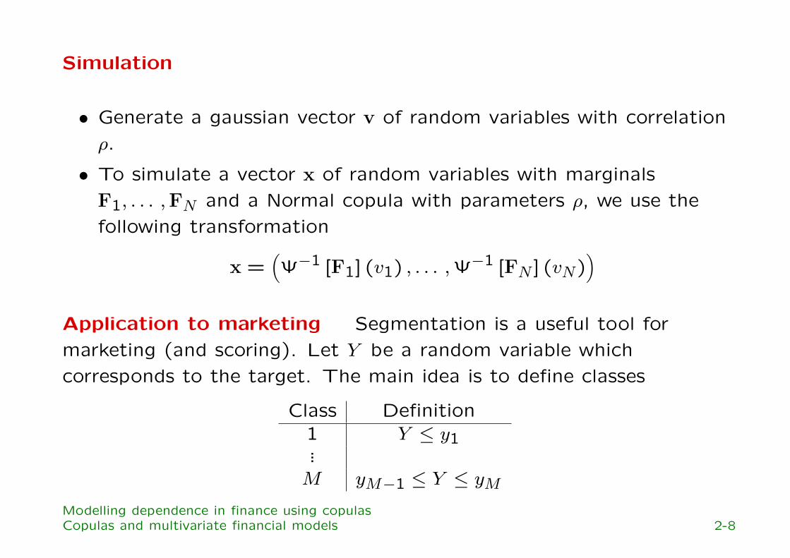
Simulation

• Generate a gaussian vector v of random variables with correlationρ.

• To simulate a vector x of random variables with marginalsF1, . . . ,FN and a Normal copula with parameters ρ, we use thefollowing transformation

x =(

Ψ−1 [F1] (v1) , . . . ,Ψ−1 [FN ] (vN))

Application to marketing Segmentation is a useful tool formarketing (and scoring). Let Y be a random variable whichcorresponds to the target. The main idea is to define classes

Class Definition1 Y ≤ y1...

M yM−1 ≤ Y ≤ yM


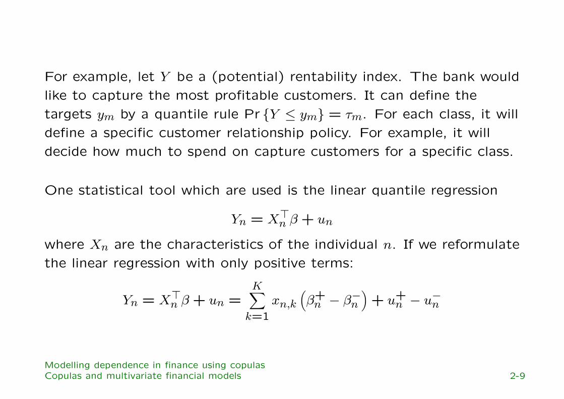
For example, let Y be a (potential) rentability index. The bank wouldlike to capture the most profitable customers. It can define thetargets ym by a quantile rule Pr Y ≤ ym = τm. For each class, it willdefine a specific customer relationship policy. For example, it willdecide how much to spend on capture customers for a specific class.

One statistical tool which are used is the linear quantile regression

Yn = X>n β + un

where Xn are the characteristics of the individual n. If we reformulatethe linear regression with only positive terms:

Yn = X>n β + un =

K∑

k=1xn,k

(

β+n − β−n

)

+ u+n − u−n


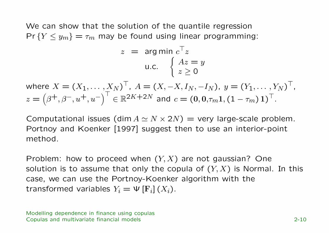
We can show that the solution of the quantile regressionPr Y ≤ ym = τm may be found using linear programming:

z = argmin c>z

u.c.

Az = yz ≥ 0

where X = (X1, . . . , XN)>, A = (X,−X, IN ,−IN), y = (Y1, . . . , YN)>,

z =(

β+, β−, u+, u−)>

∈ R2K+2N and c = (0, 0,τm1, (1− τm) 1)>.

Computational issues (dimA ' N × 2N) = very large-scale problem.Portnoy and Koenker [1997] suggest then to use an interior-pointmethod.

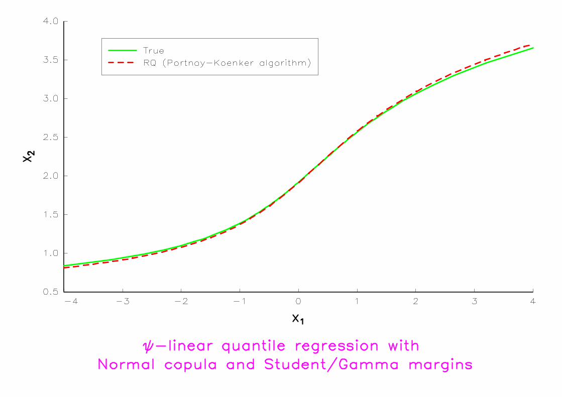
Problem: how to proceed when (Y, X) are not gaussian? Onesolution is to assume that only the copula of (Y, X) is Normal. In thiscase, we can use the Portnoy-Koenker algorithm with thetransformed variables Yi = Ψ[Fi] (Xi).


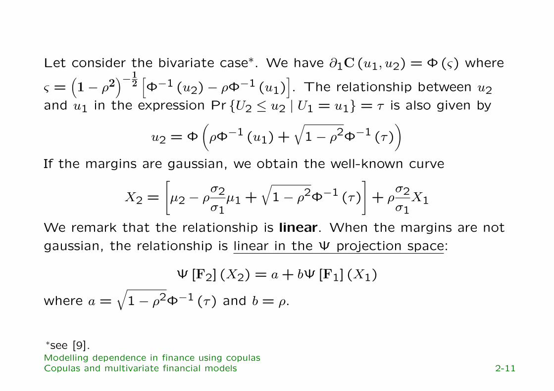
Let consider the bivariate case∗. We have ∂1C (u1, u2) = Φ(ς) where

ς =(

1− ρ2)−1

2[

Φ−1 (u2)− ρΦ−1 (u1)]

. The relationship between u2and u1 in the expression Pr U2 ≤ u2 | U1 = u1 = τ is also given by

u2 = Φ(

ρΦ−1 (u1) +√

1− ρ2Φ−1 (τ))

If the margins are gaussian, we obtain the well-known curve

X2 =

[

µ2 − ρσ2

σ1µ1 +

√

1− ρ2Φ−1 (τ)

]

+ ρσ2

σ1X1

We remark that the relationship is linear. When the margins are notgaussian, the relationship is linear in the Ψ projection space:

Ψ [F2] (X2) = a + bΨ[F1] (X1)

where a =√

1− ρ2Φ−1 (τ) and b = ρ.

∗see [9].Modelling dependence in finance using copulasCopulas and multivariate financial models 2-11

3 An open field for risk management

The bank must compute the capital needed to support the riskexposure of an operation (market, credit, operational, etc.). Ingeneral, the capital charge is determined so that the estimatedprobability of unexpected loss exhausting capital is less than sometarget insolvency rate.

Modelling dependence in finance using copulasAn open field for risk management 3-1

3.1 General framework of capital allocation

Quantile notion of the risk Let F be the (potential) lossprobability distribution (we denote ϑ the corresponding r.v.) and1− α be the target insolvency rate. The capital charge VaR (orCapital-at-Risk/Value-at-Risk) is defined by

Pr ϑ > VaR = 1− α

or by

VaR = inf x | F (x)≥ 1−α

In general, we distinguish Economic Capital (computed with internalmodels) and Regulatory Capital (computed according to methodsgiven by the Basel Commitee on Banking Supervision).


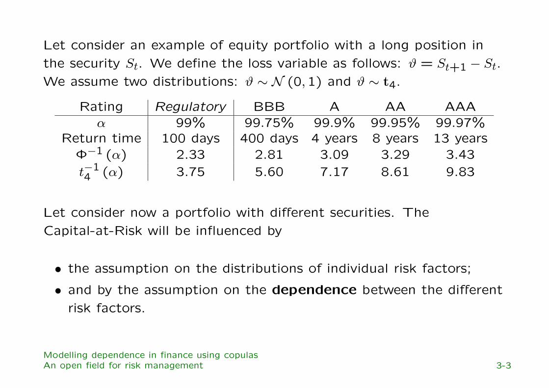
Let consider an example of equity portfolio with a long position inthe security St. We define the loss variable as follows: ϑ = St+1 − St.We assume two distributions: ϑ ∼ N (0,1) and ϑ ∼ t4.

Rating Regulatory BBB A AA AAAα 99% 99.75% 99.9% 99.95% 99.97%

Return time 100 days 400 days 4 years 8 years 13 yearsΦ−1 (α) 2.33 2.81 3.09 3.29 3.43t−14 (α) 3.75 5.60 7.17 8.61 9.83

Let consider now a portfolio with different securities. TheCapital-at-Risk will be influenced by

• the assumption on the distributions of individual risk factors;

• and by the assumption on the dependence between the differentrisk factors.


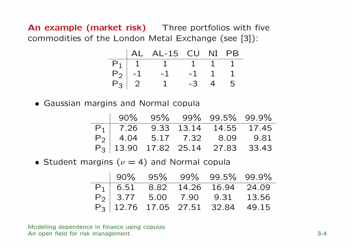
An example (market risk) Three portfolios with fivecommodities of the London Metal Exchange (see [3]):

AL AL-15 CU NI PBP1 1 1 1 1 1P2 -1 -1 -1 1 1P3 2 1 -3 4 5

• Gaussian margins and Normal copula

90% 95% 99% 99.5% 99.9%P1 7.26 9.33 13.14 14.55 17.45P2 4.04 5.17 7.32 8.09 9.81P3 13.90 17.82 25.14 27.83 33.43

• Student margins (ν = 4) and Normal copula

90% 95% 99% 99.5% 99.9%P1 6.51 8.82 14.26 16.94 24.09P2 3.77 5.00 7.90 9.31 13.56P3 12.76 17.05 27.51 32.84 49.15


3.2 Operational risk

Industry definition = “the risk of direct or indirect loss resulting frominadequate or failed internal processs, people and systems or fromexternal events” (thefts, desasters, etc.).

Operational risk is now explicitly concerned by the New Basel CapitalAccord (banks have to allocate capital for operational risk since2005).

Loss Distribution Approach (LDA) Under this approach, thebank estimates, for each business line/risk type cell, the probabilitydistributions of the severity (single event impact) and of the one yearevent frequency using its internal data. With these two distributions,the bank then computes the probability distribution of the aggregateoperational loss. The total required capital is the sum of theValue-at-Risk of each business line and event type combination.


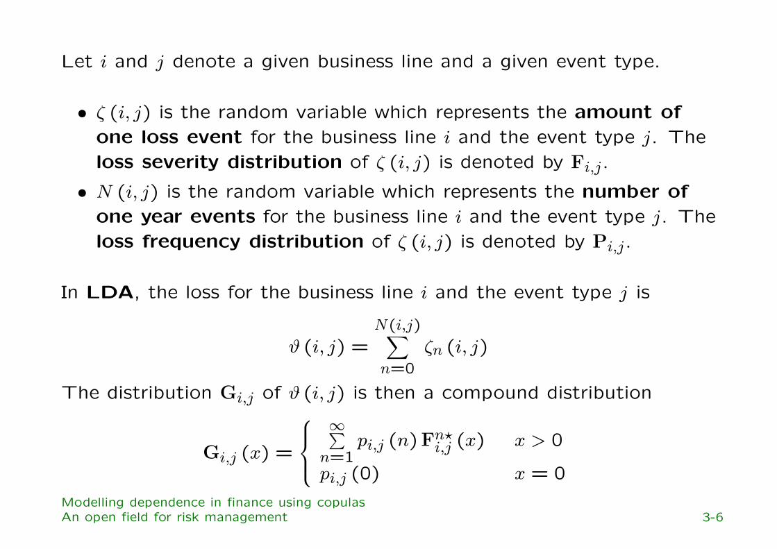
Let i and j denote a given business line and a given event type.

• ζ (i, j) is the random variable which represents the amount ofone loss event for the business line i and the event type j. Theloss severity distribution of ζ (i, j) is denoted by Fi,j.

• N (i, j) is the random variable which represents the number ofone year events for the business line i and the event type j. Theloss frequency distribution of ζ (i, j) is denoted by Pi,j.

In LDA, the loss for the business line i and the event type j is

ϑ (i, j) =N(i,j)

∑

n=0ζn (i, j)

The distribution Gi,j of ϑ (i, j) is then a compound distribution

Gi,j (x) =

∞∑

n=1pi,j (n)Fn?

i,j (x) x > 0

pi,j (0) x = 0


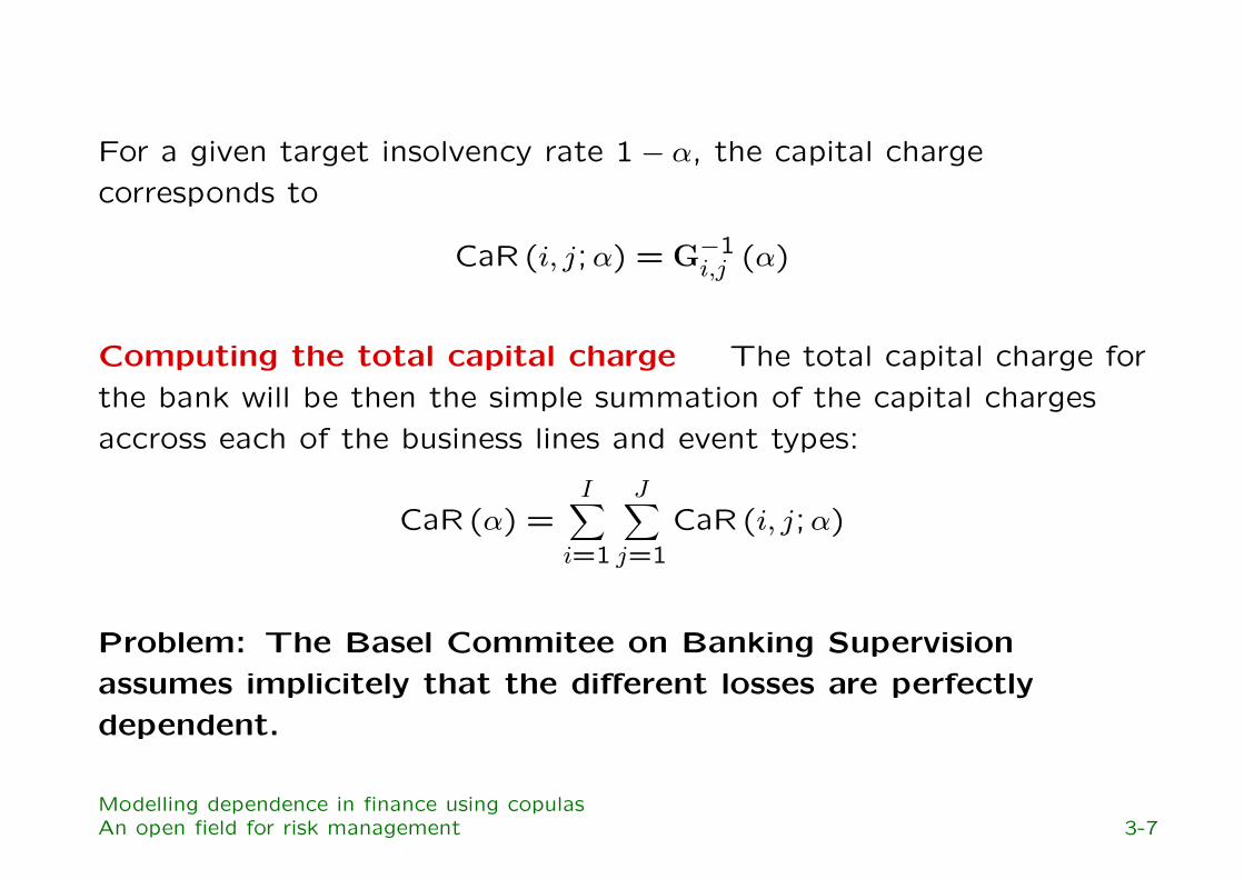
For a given target insolvency rate 1− α, the capital chargecorresponds to

CaR(i, j;α) = G−1i,j (α)

Computing the total capital charge The total capital charge forthe bank will be then the simple summation of the capital chargesaccross each of the business lines and event types:

CaR(α) =I

∑

i=1

J∑

j=1CaR(i, j;α)

Problem: The Basel Commitee on Banking Supervisionassumes implicitely that the different losses are perfectlydependent.


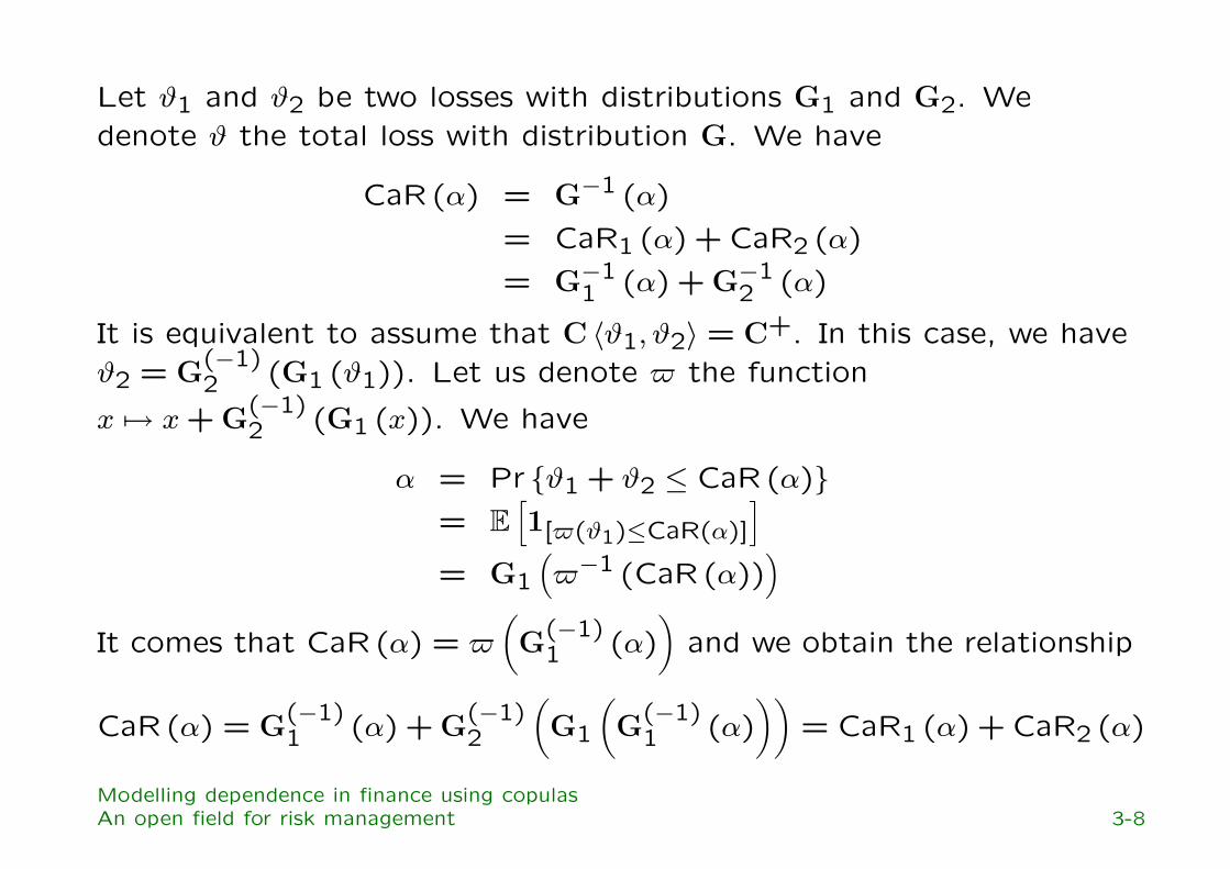
Let ϑ1 and ϑ2 be two losses with distributions G1 and G2. Wedenote ϑ the total loss with distribution G. We have

CaR(α) = G−1 (α)

= CaR1 (α) + CaR2 (α)

= G−11 (α) + G−1

2 (α)

It is equivalent to assume that C 〈ϑ1, ϑ2〉 = C+. In this case, we haveϑ2 = G(−1)

2 (G1 (ϑ1)). Let us denote $ the function

x 7→ x + G(−1)2 (G1 (x)). We have

α = Pr ϑ1 + ϑ2 ≤ CaR(α)= E

[

1[$(ϑ1)≤CaR(α)]

]

= G1(

$−1 (CaR(α)))

It comes that CaR(α) = $(

G(−1)1 (α)

)

and we obtain the relationship

CaR(α) = G(−1)1 (α) + G(−1)

2

(

G1

(

G(−1)1 (α)

))

= CaR1 (α) + CaR2 (α)


Correlated aggregate loss distributions or correlatedfrequencies? The total loss distribution ϑ for the bank as whole isdefined by

ϑ =I

∑

i=1

J∑

j=1ϑ (i, j)

In this case, we could introduce the dependence directly between theaggregate loss distributions.

Or, we could introduce the dependence indirectly between thefrequency distributions:

ϑ =I

∑

i=1

J∑

j=1

N(i,j)∑

n=0ζn (i, j)

For example, we could use multivarariate Poisson distributionsgenerated from the Normal copula (Song [2000]).


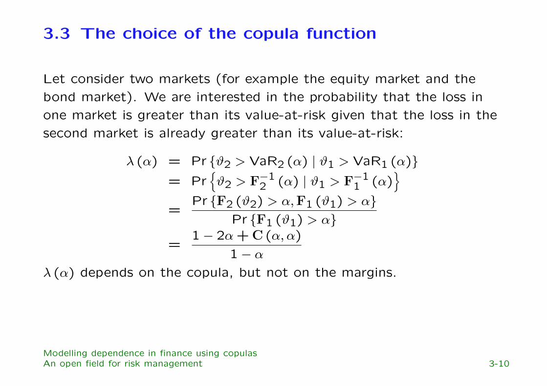
3.3 The choice of the copula function

Let consider two markets (for example the equity market and thebond market). We are interested in the probability that the loss inone market is greater than its value-at-risk given that the loss in thesecond market is already greater than its value-at-risk:

λ (α) = Pr ϑ2 > VaR2 (α) | ϑ1 > VaR1 (α)= Pr

ϑ2 > F−12 (α) | ϑ1 > F−1

1 (α)

=Pr F2 (ϑ2) > α,F1 (ϑ1) > α

Pr F1 (ϑ1) > α

=1− 2α + C (α, α)

1− αλ (α) depends on the copula, but not on the margins.


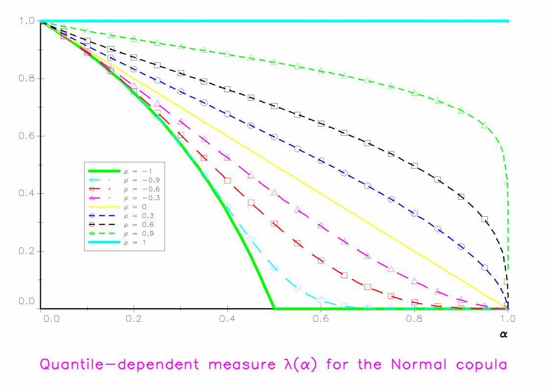
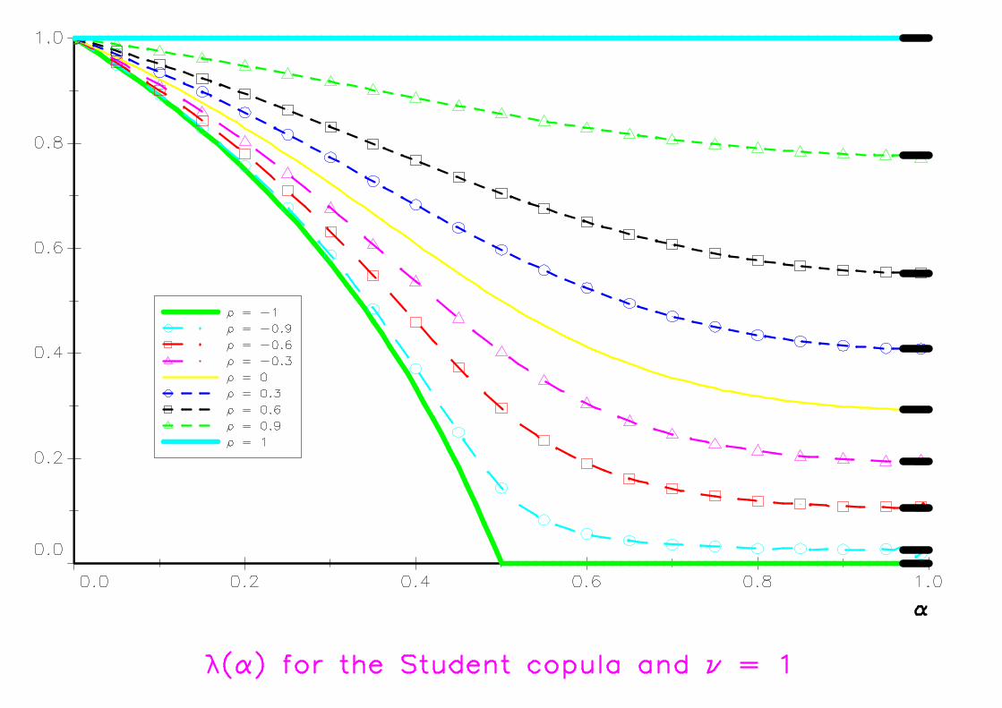
The limit case λ = limα→1 λ (α) is called the tail dependencecoefficient.

Remark 2 The measure λ is the probability that one variable isextreme given that the other is extreme.

1. Normal copula ⇒ extremes are asymptotically independent forρ 6= 1, i.e λ = 0 for ρ < 1.

2. Student copula ⇒ extremes are asymptotically dependent forρ 6= −1.

The copula function has then a great influence of the aggregation ofrisks (in particular, stress-testing is very sensitive to the choice of thecopula — see [2]).


4 New pricing methods with copulas

Let consider an European Call option. The payoff isG (T ) = (S (T )−K)+. Under some conditions, the price P (t0) of thiscontingent claim is given by

P (t0) = e−r(T−t0)EQ[

G (T )| Ft0

]

with Q the martingale probability measure.

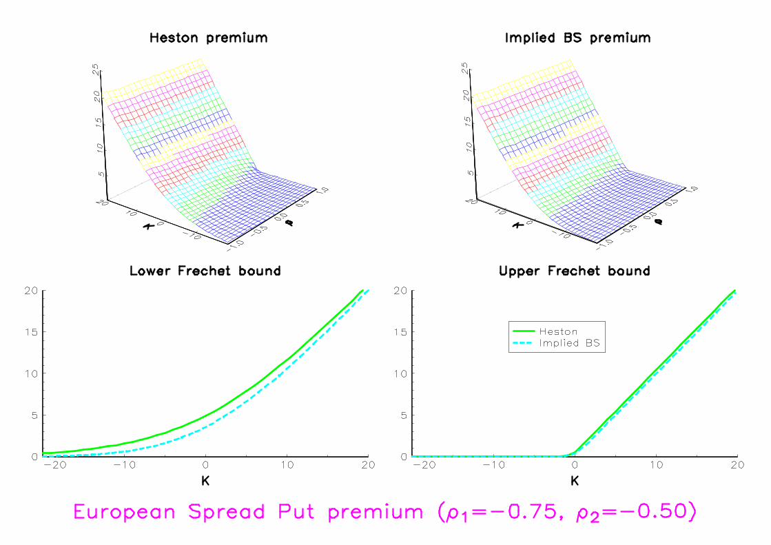
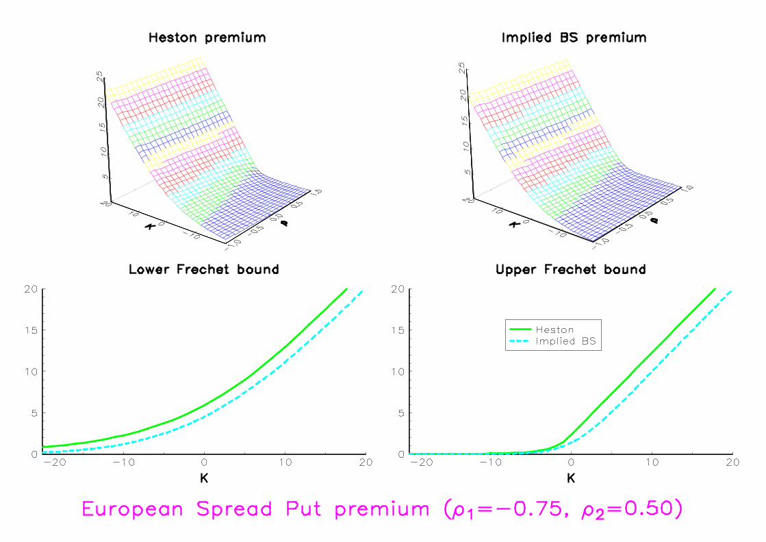
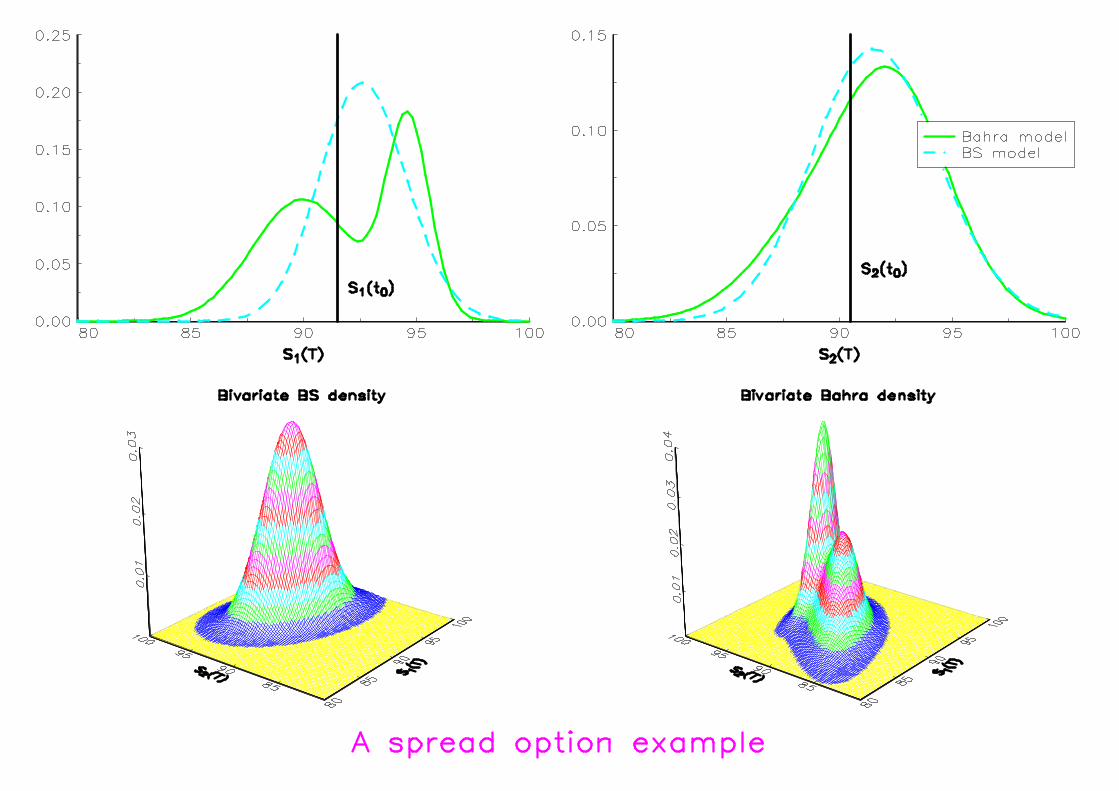
For a spread option, we have G (T ) = (S2 (T )− S1 (T )−K)+ and weobtain a similar expression for the price.

Spread option is a special case of two-asset options. Since someyears, multi-asset options are traded very frequently. The maindifference with option with only one underlying is that the martingaleprobability measure is multidimensional.

Modelling dependence in finance using copulasNew pricing methods with copulas 4-1

4.1 Coherent valuation of multi-asset options

The Black-Scholes model In the BS model, we have

dS (t) = rS (t) dt + σS (t) dW (t)

under Q. The price of an European option is then a function of thevolatility σ. However, when we compute the implied volatility fromthe option prices for different values of the strike K, it is notconstant. This is the volatility smile effect.

Option models in banks Banks have then developpedsophisticated models (e.g. stochastic volatility models) to take intoaccount the smile effect.

To this day, therefore, the BS model continues to be used, out ofanalytical and computational convenience, for contingent claimsbased on different assets.


Problem: the margins of the multivariate Risk-Neutral Distribution(RND) are not the univariate RND.

⇒ In this case, we may show that there exists arbitrage opportunitiesinside the same bank (see [10]).

⇒ Moreover, one-asset options could be viewed as limits ofmulti-asset options — see e.g. the Basket optionG (T ) = (α1S1 (T ) + α2S2 (T )−K)+.

The copula construction Let Q be the multivariate RND of therandom vector S (T ) | Ft0. In [10], we show that the margins of Q arenecessarily univariate RND∗. Using Sklar’s theorem, it comes that Qadmits the following canonical decomposition

Q (S1 (T ) , . . . , SN (T )) = CQ (Q1 (S1 (T )) , . . . ,QN (SN (T )))

CQ is called the risk-neutral copula (RNC).∗We prove this by using properties of the Girsanov theorem applied to multivariateprobability measure.


Relationships between CQ and CP

Let P be the objective (or historical) distribution. We denote by CP

the objective copula. We can prove the following proposition:

Proposition 1 If the drift and the diffusion of the asset prices vectorS (t) are of the form µ (t) S (t) and σ (t) S (t) and if risk premiumsare non stochastic, then the risk-neutral copula CQ is equal to theobjective copula CP.

Implication of this proposition: in this case, the univariate RND canbe estimated using the options market whereas the RNC can beestimated using the spot market. So, the spot market contains usefulinformation to price multi-asset options.


The case of the spread option In [12], Valdo Durrleman showsthat the price P (t0) is

P (t0) = S2 (t0)− S1 (t0)−Ke−r(T−t0) +

e−r(T−t0)∫ K

−∞

∫ +∞

0f1 (x) · ∂1CQ (F1 (x) ,F2 (x + y)) dxdy

A remark The copula construction implies that we can associatea risk-neutral copula to a multivariate risk-neutral distribution. But itdoes not mean that the combination of univariate RND with a copuladefine necessarily a multivariate risk-neutral distribution (see [10] forfurther details).


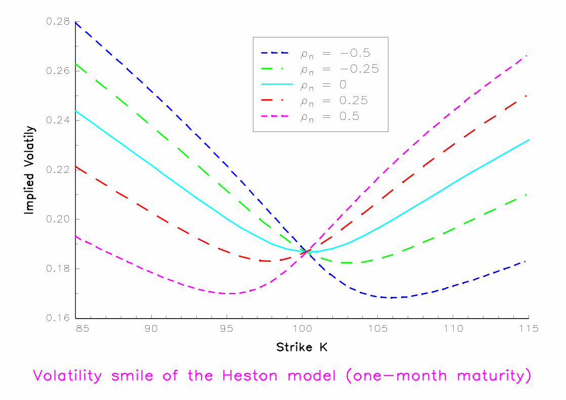
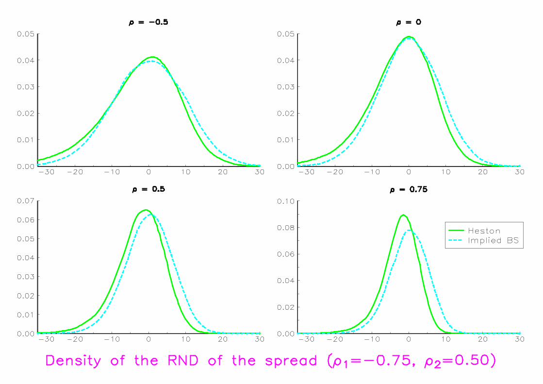
BS pricing in stochastic volatility environment We assumethat the asset prices Sn (t) are given by the Heston model

dSn (t) = µnSn (t) dt +√

Vn (t)Sn (t) dW1n (t)

dVn (t) = κn (Vn (∞)− Vn (t)) dt + σn√

Vn (t) dW2n (t)

with E[

W1n (t)W2

n (t) | Ft0

]

= ρn (t− t0), κn > 0, Vn (∞) > 0 andσn > 0. The market prices of risk processes areλ1

n (t) = (µn − r) /√

Vn (t) and λ2n (t) = λnσ−1

n

√

Vn (t).

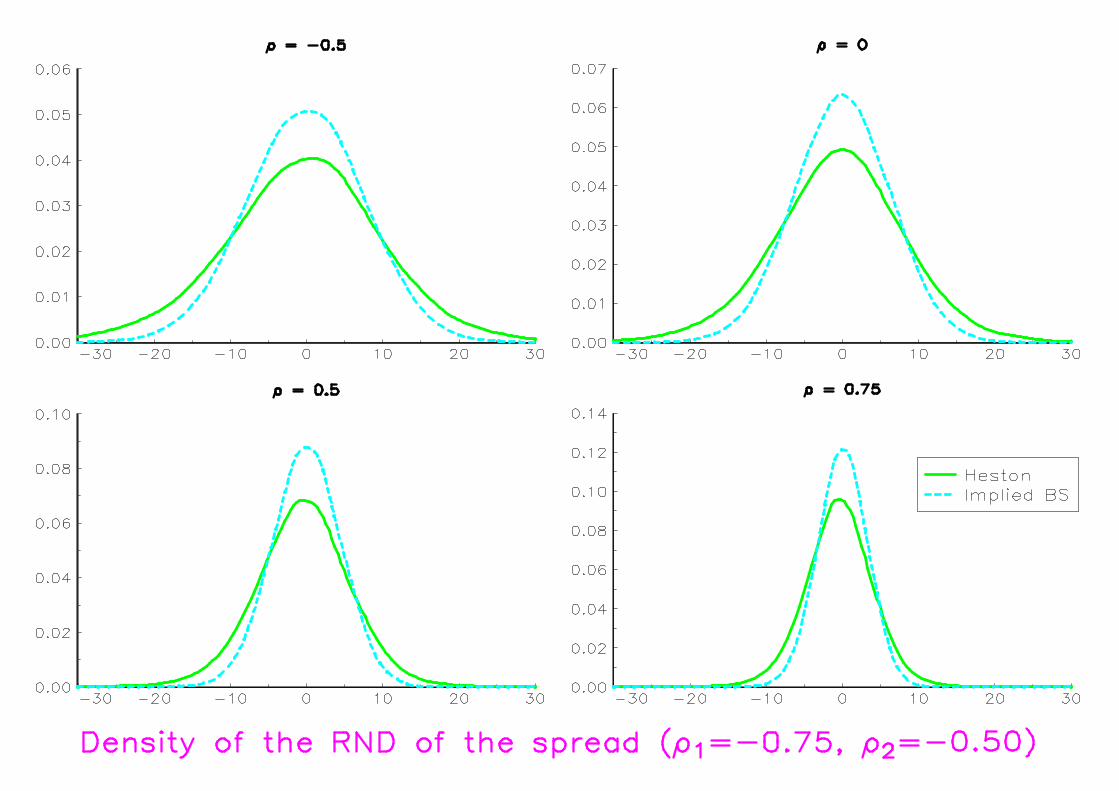
To compute prices of spread options, we consider that the RNC is theNormal copula with parameter ρ. We compare then the Heston priceswith these given by the BS model using ATM implied volatilities.

Numerical values (two assets with same characteristics except ρn):Sn (t0) = 100, τ = 1/12, r = 5%, Vn (t0) = Vn (∞) =

√20%, κn = 0.5,

σn = 90% and λn = 0.


How to build ‘forward-looking’ indicators for the dependencefunction?

In [1], Aris Bikos suggests the following method:

1. estimate the univariate RND Qn using Vanilla options;

2. estimate the copula C using multi-asset options by imposing thatQn = Qn;

3. derive “forward-looking” indicators directly from C.


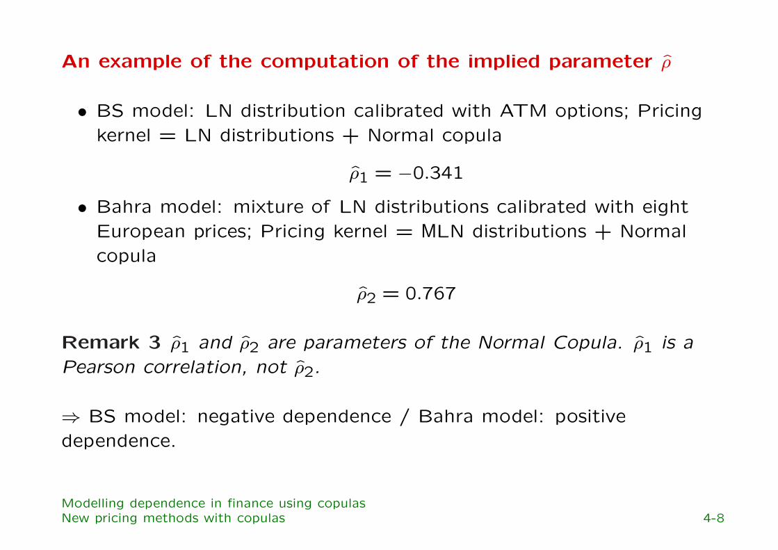
An example of the computation of the implied parameter ρ

• BS model: LN distribution calibrated with ATM options; Pricingkernel = LN distributions + Normal copula

ρ1 = −0.341

• Bahra model: mixture of LN distributions calibrated with eightEuropean prices; Pricing kernel = MLN distributions + Normalcopula

ρ2 = 0.767

Remark 3 ρ1 and ρ2 are parameters of the Normal Copula. ρ1 is aPearson correlation, not ρ2.

⇒ BS model: negative dependence / Bahra model: positivedependence.


4.2 The pricing of credit derivativesIn multi-asset options, the risk is a market risk (because of thevolatility of the asset prices). In credit derivatives, the risk is a creditrisk (because of the default of the counterparties).

A default is generally described by a survival functionS (t) = Pr T > t. Let C be a survival copula. A multivariate survivalfunction S can be defined as follows

S (t1, . . . , tN) = C (S1 (t1) , . . . ,SN (tN))

where (S1, . . . ,SN) are the marginal survival functions. Nelsen [1999]notices that “C couples the joint survival function to its univariatemargins in a manner completely analogous to the way in which acopula connects the joint distribution function to its margins”.

⇒ Introducing dependence between defaultable securities can then bedone using the copula framework (see [21] and [25]).


Some examples∗

The Default Digital Put (DDP) option

The European DDP “pays off 1 at t iff there has been a default atsome time before (or including) t”.

If we assume that the interest rate and the first default τ =∧N

n=1 Tnare independent, the price at time t0 of the DDP of maturity t isthen†

DDP (t0, t) = E[

e−

∫ tt0

r(s) ds1[τ<t]

]

= (1− Sτ (t))P (t0, t)=

(

1− C (S1 (t) , . . . ,SN (t)))

P (t0, t)

∗These examples are taken from [18].†P (t0, t) is the default-free bond price.Modelling dependence in finance using copulasNew pricing methods with copulas 4-10

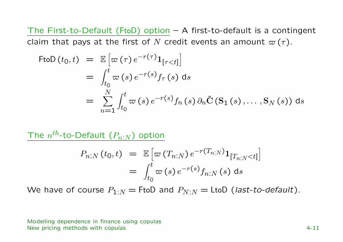
The First-to-Default (FtoD) option – A first-to-default is a contingentclaim that pays at the first of N credit events an amount $ (τ).

FtoD (t0, t) = E[

$ (τ) e−r(τ)1[τ<t]

]

=∫ t

t0$ (s) e−r(s)fτ (s) ds

=N∑

n=1

∫ t

t0$ (s) e−r(s)fn (s) ∂nC (S1 (s) , . . . ,SN (s)) ds

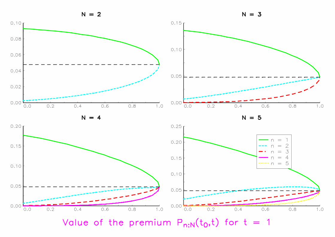
The nth-to-Default (Pn:N) option

Pn:N (t0, t) = E[

$ (Tn:N) e−r(Tn:N)1[Tn:N<t]

]

=∫ t

t0$ (s) e−r(s)fn:N (s) ds

We have of course P1:N = FtoD and PN :N = LtoD (last-to-default).


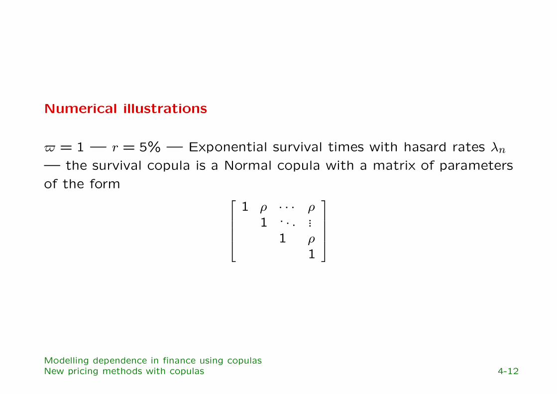
Numerical illustrations

$ = 1 — r = 5% — Exponential survival times with hasard rates λn

— the survival copula is a Normal copula with a matrix of parametersof the form

1 ρ · · · ρ1 .. . ...

1 ρ1


5 Conclusion

The use of copulas in finance is very recent.

However, private communications with professionals of other banksindicate that copulas are largely studied (and used) in most banks.

And professionals expect a lot from copulas to solve (andunderstand) many financial problems.

Modelling dependence in finance using copulasConclusion 5-1

6 References (Copulas and Finance)

[1] Bikos, A. [2000], Bivariate FX PDFs: a Sterling ERI application, Bank of England, WorkingPaper

[2] Bouye, E., V. Durrleman, A. Nikeghbali, G. Riboulet and T. Roncalli [2000], Copulas forfinance — a reading guide and some applications, Groupe de Recherche Operationnelle, CreditLyonnais, Working Paper

[3] Bouye, E., V. Durrleman, A. Nikeghbali, G. Riboulet and T. Roncalli [2000], Copulas: an openfield for risk management, Groupe de Recherche Operationnelle, Credit Lyonnais, WorkingPaper

[4] Bouye, E., N. Gaussel and M. Salmon [2000], Investigating dynamic dependence using copulae,Financial Econometric Research Centre, City University Business School, Working Paper

[5] Ceske, R. and J.V. Hernandez [1999], Where theory meets practice, Risk Magazine(Operational Risk Report), 12, November, 17-20

[6] Ceske, R., J.V. Hernandez and L.M. Sanchez [2000], Quantifying event risk: the nextconvergence, The Journal of Risk Finance, 1(3), 9-23

[7] Cherubini, U. and E. Luciano [2000], Multivariate option pricing with copulas, University ofTurin, Working Paper

[8] Cherubini, U. and E. Luciano [2000], Value at risk trade-off and capital allocation withcopulas, University of Turin, Working Paper

Modelling dependence in finance using copulasReferences (Copulas and Finance) 6-1

[9] Costinot, A., T. Roncalli and J. Teiletche [2000], Revisiting the dependence between financialmarkets with copulas, Groupe de Recherche Operationnelle, Credit Lyonnais, Working Paper

[10] Coutant, S., V. Durrleman, G. Rapuch and T. Roncalli [2001], Copulas, multivariaterisk-neutral distributions and implied dependence functions, Groupe de RechercheOperationnelle, Credit Lyonnais, Working Paper

[11] Coutant, S., P. Martineu, J. Messines, G. Riboulet and T. Roncalli [2001], Credit riskmodelling with copulas, Groupe de Recherche Operationnelle, Credit Lyonnais, Working Paper

[12] Durrleman, V. [2001], Implied correlation and spread options, Princeton University, WorkingPaper

[13] Durrleman, V., A. Nikeghbali and T. Roncalli [2000], How to get bounds for distributionconvolutions? A simulation study and an application to risk management, Groupe deRecherche Operationnelle, Credit Lyonnais, Working Paper

[14] Embrechts, P., A.J. McNeil and D. Straumann [1999], Correlation and dependency in riskmanagement: properties and pitfalls, ETH Zurich, Working Paper

[15] Embrechts, P., A. Hoeing and A. Juri [2001], Using copulae to bound the value-at-risk forfunctions of dependent risk, ETH Zurich, Working Paper

[16] Frachot, A., P. Georges and T. Roncalli [2001], Loss Distribution Approach for operationalrisk, Groupe de Recherche Operationnelle, Credit Lyonnais, Working Paper

[17] Frey, A. and A.J. McNeil [2000], Modelling dependent defaults, ETH Zurich, Working Paper

[18] Georges, P., A-G. Lamy, E. Nicolas, G. Quibel and T. Roncalli [2001], Multivariate survivalmodelling: a unified approach with copulas, Groupe de Recherche Operationnelle, CreditLyonnais, Working Paper

[19] Giesecke, K. [2001], Structural modeling of correlated defaults with incomplete information,Humboldt-Universitat zu Berlin, Working Paper

[20] Hamilton, D., J. James and N. Webber [2001], Copula methods and the analysis of credit risk,University of Warwick, Working Paper (original version December 2000)

[21] Li, D.X. [2000], On default correlation: a copula function approach, Journal of Fixed Income,9(4), 43-54

[22] Lindskog, F. [2000], Modelling dependence with copulas, ETH Zurich, Master Thesis

[23] Lindskog, F. and A.J. McNeil [2001], Common poisson shock models, RiskLab, Research Paper

[24] Luciano, E. and M. Marena [2001], Value at risk bounds for portfolios of non-normal returns,University of Turin, Working Paper

[25] Maccarinelli, M. and V. Maggiolini [2000], The envolving practice of credit risk management inglobal financial institutions, Risk Conference, 26/27 September, Paris

[26] Malevergne, Y. and D. Sornette [2001], General framework for a portfolio theory withnon-Gaussian risks and non-linear correlations, University of Nice, Working Paper

[27] Patton, A. [2000], Modelling time-varying exchange rate dependence using the conditionalcopula, University of California, San Diego, Working Paper

[28] Rockinger, M. and E. Jondeau [2001], Conditional dependency of financial series: anapplication of copulas, Groupe HEC, Cahier de Recherche, 723/2001

[29] Rosenberg, J.V. [1999], Semiparametric pricing of multivariate contingent claims, Stern Schoolof Business, Working Paper, S-99-35

[30] Rosenberg, J.V. [2000], Nonparametric pricing of multivariate contingent claims, Stern Schoolof Business, Working Paper, FIN-00-001

[31] Scaillet, O. [2000], Nonparametric estimation of copulas for time series, Universite Catholiquede Louvain, Working Paper

[32] Schonbucher, P.J. and D. Schubert [2001], Copula-dependent default risk in intensity models,Bonn University, Working Paper

[33] Tibiletti L. [2000], Incremental value at risk and VaR with background-risk: traps andmisinterpretations, University of Turin, Working Paper

7 Other references

[1] Deheuvels, P. [1978], Caracterisation complete des lois extremes multivariees et de laconvergence des types extremes, Publications de l’Institut de Statistique de l’Universite deParis, 23, 1-36

[2] Genest, C., K. Ghoudi and L-P Rivest [1995], A semiparametric estimation procedure fordependence parameters in multivariate families of distributions, Biometrika, 82(3), 543-552

[3] Genest, C. and J. MacKay [1986], Copules archimediennes et familles de lois bidimensionnellesdont les marges sont donnees, Canadian Journal of Statistics, 14(2), 145-159

[4] Joe, H. and J.J. Xu [1996], The estimation method of inference functions for margins formultivariate models, Department of Statistics, University of British Columbia, TechnicalReport, 166

[5] Nelsen, R.B. [1998], An Introduction to Copulas, Lectures Notes in Statistics, 139, SpringerVerlag, New York

[6] Schweizer, B. and E. Wolff [1981], On nonparametric measures of dependence for randomvariables, Annals of Statistics, 9, 879-885

[7] Song, P. X-K. [2000], Multivariate dispersion models generated from Gaussian copula,Scandinavian Journal of Statistics, 27-2, 305-320

Modelling dependence in finance using copulasOther references 7-1

modelling dependence in ﬁnance using...

Documents