modelling and quasistatic simulation of the stiffness

Ope n Pe e r Re v ie w on Qe iosOpe n Pe e r Re v ie w on Qe ios

Modelling and quasistatic simulation ofthe stiffness degradation of concretebased on physical measurements

Jürgen Ries

Abstract

AIM:

T he description of the mechanical properties of concrete is usually done with two

pairs of values "stress-strain" within the "elastic area" which are defining the slope

(Young's modulus) and the peak value (strength). T he post-peak-behaviour

(softening) is usually defined only by a theory giving the decreasing curve e.g.

exponential softening. T herefore the aim of this project is the metrological

recording of the complete stress-strain-curve for the integration into the material

model, reproducing the "linear" and the nonlinear area (softening) within the

nonlinear simulation exactly.

T he quality of simulation results should improve when using physical measured

values as input data of the material model.

PROCEDURE:

According to the statistical evaluation of the experimentally determined material

parameters (compressive-, bending -, tensile-, splitting tensile strength), the bending

strength was identified as the material parameter with the least deviation from the

mean value (relative scattering coefficient, the coefficient of variation). T his leads to

the objective of implementing the electronically recorded measurement data of the

carried out deformation controlled 4-point-bending-tests (according to test

guideline German committee for reinforced concrete DAfStB) into the material

model. T he experimentally recorded forces and displacements were linearly

converted into normalized stresses and strains according to the rules of statics. T he

input for the elastic-degrading material model of the steel-fibre-concrete are 20

pairs of values, taken from the measured data of the 4-point bending test.

T he material model (smeared cracking method) of the unreinforced fibre concrete

and it’s softening is thus based exclusively on experimentally measured data, taken

from the 4-point-bending-tests. T he theoretical material models available in "Ansys

Mechanical", e.g. “Mohr-Coulomb” or “Drucker-Prager”, have not been applied here.

Qeios, CC-BY 4.0 · Article, May 8, 2019

Qeios ID: 649497 · https://doi.org/10.32388/649497 1/19

https://www.qeios.com/read/article/279#reviews

https://www.qeios.com/profile/1340

T he usual input data of the uniaxial tensile- and compressive strength were also not

included in the simulation.

When evaluating the 4-point tests, the lowest force-displacement curve is decisive

(minimum work performed); this corresponds to the main crack in midspan. In the

area of the damage between the load applications, the constant (bending) normal-

stress corresponds to the equivalent stress because of the lack of (bending) shear-

stress. T he (bending) normal-stress together with the plastic strain are the

experimental input values of the material model.

CONCLUSION:

Element size and deformation rate have to be minimal for a good quality simulation

result. T here are deviations between simulation and experiment in the „elastic zone“

and also concerning the peak value (bending strength) because within the simulation

all cracks are smeared homogeneously.

Sufficient local and temporal discretization / sufficient small mesh size and

deformation speed bring the nonlinear simulation close to the physical reality. T he

optimum quality of results is achieved with a specific mesh density and a specific

deformation speed - too small values, on the other hand, will worsen the quality of

results (optimization process). T he elastic-degrading/multilinear-elastic simulation

using a physically based material model showed no convergence problems.

1 . Mat er i a l Model1 . Mat er i a l ModelBased on 4-point bending experiments (beam 15x15x70cm)Based on 4-point bending experiments (beam 15x15x70cm)

T he statistic analysis of the material parameters, determined by experiments with the

small specimen, delivered the following „coefficient of variation“ results for steel-fibre-

concrete C30/37 containing 25kg/m³ steel fibres and 0,5kg/m³ plastic fibres.

Figure 1: Mean scatter of the material parameters for the preferenced concrete mix (COV coefficient of

variation [%])

T he bending tensile strength can be identified as the material parameter with the lowest

coefficient of variation. T herefore, according to the project‘s aim, the electronic



measured data of the 4-point-bending-tests (test guideline "Steel fibre concrete" of the

"DAFStB german committee for reinforced concrete") is implemented in the material

model.

Figure 2: 4-point bending experiment, deformation-controlled , beam 15x15x70cm, span length 60cm,

test duration about 20min, test guideline "Steel fibre concrete" of the "German committee for reinforced

concrete DAfStB"

T he recorded experimental forces and displacements have been converted to

normalized stress and strain data acc. the rules of statics. T wenty experimental pairs of

values have been recalculated to stress-strain data and implemented into a multi-linear-

elastic material model.

T herefore the material model of the steel-fibre-concrete is only based on the

measurements of the 4-point-bending-tests. T heoretic material models provided by

„Ansys Mechanical“ have not been used. No uniaxial tensile strength resp. compressive

strength has been included in the model.

Figure 3: Input data in Ansys „Mela“ for the elastic-degrading material model of the steel-fibre-concrete.



20 pair of values force-displacement (4-point-bending experiment) have been recalculated to stress-

strain data.

Please find here a short video file (1min) of the 4-point-bending experiment:

https://www.researchgate.net/profile/Juergen_Ries

Subsequent some figures concerning the quasistatic simulation of the 4-point bending

test.

Figure 4: Side view, first principal stress



Figure 5: Bottom view, first principal stress

Figure 6: Side view, equivalent stress



Figure 7: Bottom view, equivalent stress

Figure 8: Side view, first plastic strain



Figure 9: Bottom view, first plastic strain

Figure 10: Comparison between experimental data and the theory of „Bach-Schüle“

T he power law from Bach and Schüle

σn = E ∗ ϵ is very close to the experimental curve and describes the softening of the

concrete very well.

Within the evaluation of the 4-point-bending tests, the lowest force-displacement-curve

is decisive (minimal serviced work); this refers to the main crack in midspan.



Figure 11: Main crack located in the mid-span and symmetric area of degradation

Acc. to the rules of static there is a constant bending moment between the applied loads,

but there is no shear force. T he area of degradation spreads out uniformly to the left

and right side of the main crack located in midspan. In the area of damage between the

applied loads, the normal stress from bending equals the equivalent stress - because of

the missing shear stress. Normal stress and plastic strain represent the input values of

the material model.

T he next graph shows the simulation/verification of the 4-point-bending-test. All implicit

simulations within this article have been done in Ansys Mechanical.

Figure 12: Experiment and quasistatic simulation of the 4-point-bending-test done in „Ansys

Mechanical“; the calculation time increases with decreasing deformation step / with increasing time

discretization.

Element size and deformation rate have to be minimal for a good quality simulation

result. T here are deviations between simulation and experiment in the „elastic zone“ and



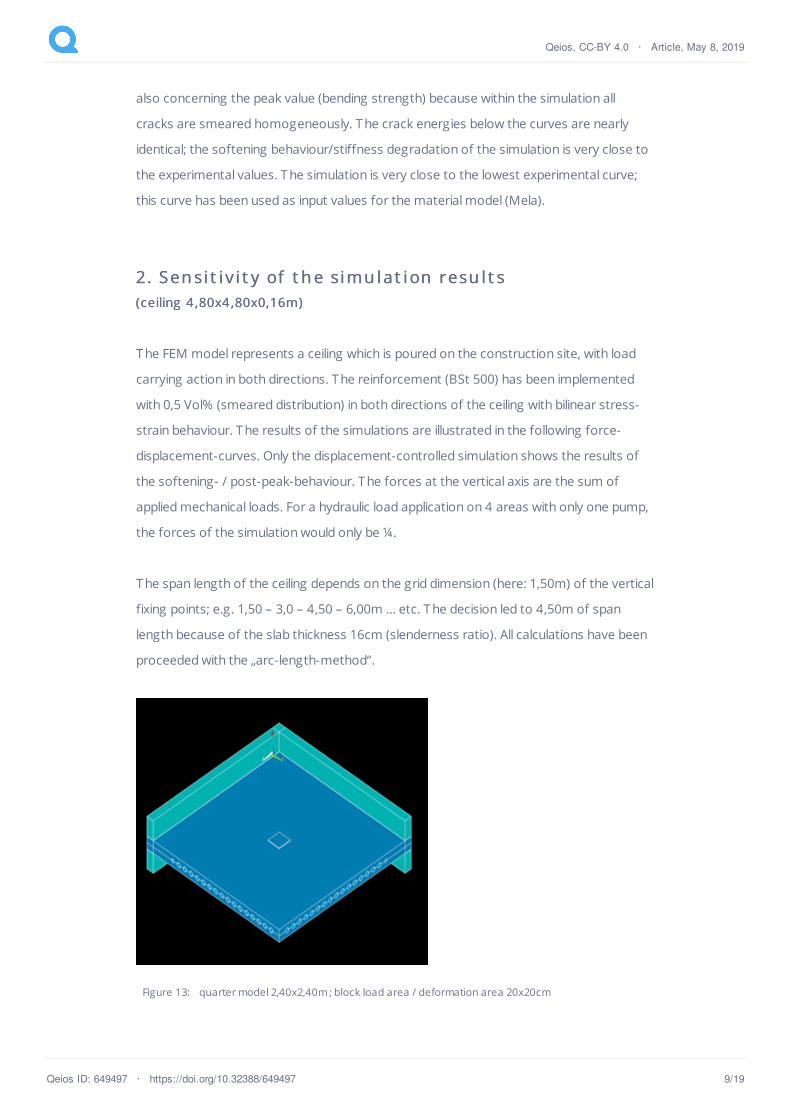
Figure 13: quarter model 2,40x2,40m ; block load area / deformation area 20x20cm

also concerning the peak value (bending strength) because within the simulation all

cracks are smeared homogeneously. T he crack energies below the curves are nearly

identical; the softening behaviour/stiffness degradation of the simulation is very close to

the experimental values. T he simulation is very close to the lowest experimental curve;

this curve has been used as input values for the material model (Mela).

2. Sen si t i v i t y of t h e si mu l at i on resu l t s2. Sen si t i v i t y of t h e si mu l at i on resu l t s(ceiling 4 ,80x4 ,80x0,16m)(ceiling 4 ,80x4 ,80x0,16m)

T he FEM model represents a ceiling which is poured on the construction site, with load

carrying action in both directions. T he reinforcement (BSt 500) has been implemented

with 0,5 Vol% (smeared distribution) in both directions of the ceiling with bilinear stress-

strain behaviour. T he results of the simulations are illustrated in the following force-

displacement-curves. Only the displacement-controlled simulation shows the results of

the softening- / post-peak-behaviour. T he forces at the vertical axis are the sum of

applied mechanical loads. For a hydraulic load application on 4 areas with only one pump,

the forces of the simulation would only be ¼.

T he span length of the ceiling depends on the grid dimension (here: 1,50m) of the vertical

fixing points; e.g. 1,50 – 3,0 – 4,50 – 6,00m … etc. T he decision led to 4,50m of span

length because of the slab thickness 16cm (slenderness ratio). All calculations have been

proceeded with the „arc-length-method“.



Figure 14: quarter model 2,40x2,40m ; view inside the CC-structures of the ceiling

Figure 15: Influence of mesh size (LESIZE) and load case – the displacement controlled simulations

show the softening after the peak of the load; the calculation time increases with decreasing element

size / with increasing geometric discretization (LESIZE).



Figure 16: Influence of the element size/mesh size: with smaller mesh size the simulation converges

towards the physical reality; the calculation time increases with decreasing element size / with

increasing geometric discretization (LESIZE).

Figure 17: three different load scenarios: only with the displacement-controlled simulation the

softening can be shown, the force-controlled simulations converge only pre-peak.



Figure 18: Influence of deformation rate: the deformation rate has to be small enough as well, to

receive a simulation result near to physical reality; the calculation time increases with decreasing

deformation step / with increasing time discretization.

Figure 19: Comparison of the massive and hollow ceiling, the prediction for the experiment



T ill about 300KN (15KN/m²) the massive and the hollow construction can be seen as

equivalent, the curves are parallel to each other. T he massive construction will hold a

higher load level for >400KN. T his load level won’t be reached in reality, for normal use

the level is scheduled with 5KN/m² (100KN). T he degree of restraint of the simulated

supports has to be calibrated with the experimental strain measurements along the

supports.

With smaller mesh size and smaller deformation rate, the simulation will get closer to

physical reality. T he boundary conditions of the simulation have to be calibrated with the

experimental strain measurements along the supports. T he elastic degrading/multilinear

elastic simulation using a physically based material model showed no convergence

problems. T he physically measured strains at the upper side of the ceiling

(photogrammetry) will be compared with the simulated values; the differences will show

good and bad areas. Finally, optimization potentials can be identified by specifying the

origin of the differences.

T he element size converged at LESIZE=3cm, the deformation step size converged at

0,1mm. T he increase of local discretization or time discretization / the reduction of mesh

size or deformation step size (time step size) will minimize the strain energy – the

physical process will be reproduced.

Up to the target value (element size 3cm or deformation rate 0,1mm), the simulation

results showed the behaviour of a monotonic convergence. When the target value was

exceeded, the behaviour of the results changed to an oscillating convergence, which in

turn severely degraded the quality of the results.

Subsequent some pictures of the last simulation / prediction for the experiment

(LESIZE=0.03m deformation step=0.1mm). T he print of displacement is 10x inflated.



Figure 20: Top side, first principal stress

Figure 21: Lower side, first principal stress



Figure 22: Top side, first plastic strain

Figure 23: Lower side, first plastic strain



Figure 24: Top side, equivalent stress

Figure 25: Lower side, equivalent stress



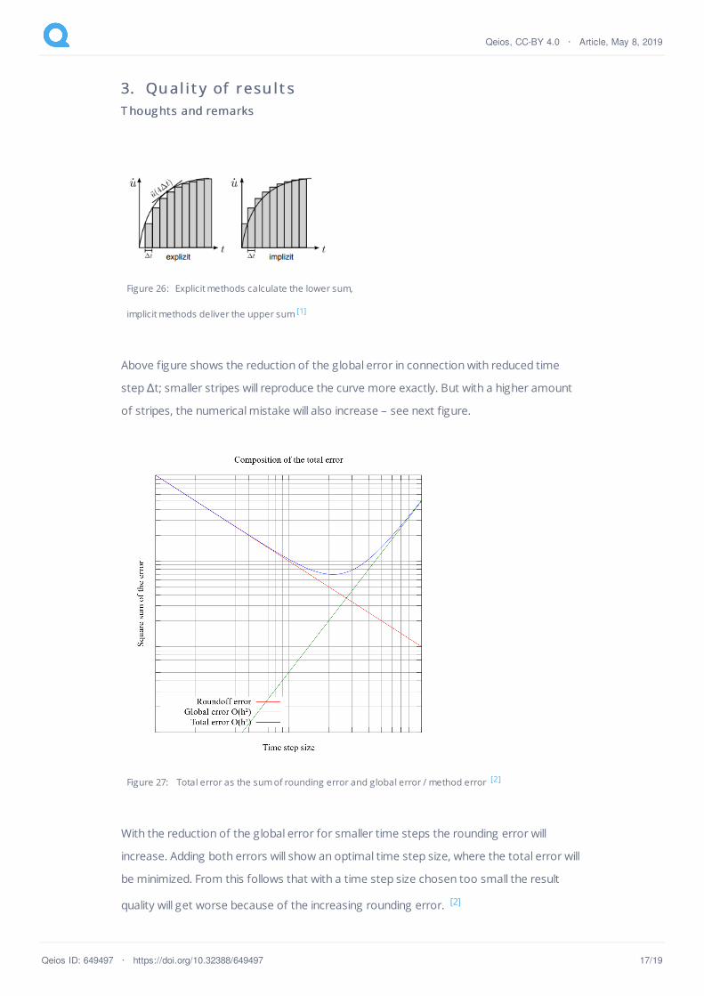
3. Qu al i t y of resu l t s3. Qu al i t y of resu l t sT houg hts and remarksT houg hts and remarks

Figure 26: Explicit methods calculate the lower sum,

implicit methods deliver the upper sum [1]

Above figure shows the reduction of the global error in connection with reduced time

step ∆t; smaller stripes will reproduce the curve more exactly. But with a higher amount

of stripes, the numerical mistake will also increase – see next figure.

Figure 27: Total error as the sum of rounding error and global error / method error [2]

With the reduction of the global error for smaller time steps the rounding error will

increase. Adding both errors will show an optimal time step size, where the total error will

be minimized. From this follows that with a time step size chosen too small the result

quality will get worse because of the increasing rounding error. [2]



T his relationship should also be valid for the element size – with smaller element size the

rounding error will increase while the global error/method error will decrease. T herefore

too small element sizes will worsen the result quality because of the increasing total

error.

4 . Su mmary an d ou t l ook4 . Su mmary an d ou t l ook

With decreasing element size or deformation speed, the simulation gets closer to

physical reality. Reducing these parameters over a certain level the force-displacement-

curve did not get lower anymore and took place above the last curve – this behaviour has

to be reviewed more exactly in future research projects. T he optimal result quality with a

minimized total error can be reached with certain values for element size and

deformation speed; these parameters have to be found. T he exceeding of these optimal

parameters has to be avoided; choosing an element size or deformation speed too small

will cause a significant worsening of the total result quality. T he origin of the abrupt

worsening result quality should have it’s source within the increasing numerical error of

the calculation; with decreasing element size or time step (deformation step/load step)

the numerical error increases.

Choosing the discretization of geometry or time will depend on the system stiffness. For

a short beam, the parameters have to be much smaller compared to a ceiling with larger

span length; e.g. applicable evaluation criteria could be the slenderness ratio. Even within

the implicit quasistatic analysis, the discretization of time by deformation step or load

step has a big influence on the simulation result. T herefore the quasistatic simulation has

to be seen as a time-dependent simulation.

H ypothesisH ypothesis ::

T he author formulates the hypothesis, that the convergence concerning the

deformation speed (here: 0,1mm) results from the deformation speed of the 4-point-

bending experiment. T he experimental curve of the 4-point-bending test is time-

dependent; the usage as the input of the material model transfers the damping

behaviour of the concrete to the model. T he equation of motion includes the velocity as

the first derivative of movement. T his means the only unknown variable in the model is

the discretization of geometry / the element size.

More detailed information concerning the project „CC-technology“ can be found here:



https://www.researchgate.net/profile/Juergen_Ries

T he references have been translated by the author.

References

1. ^ Simon Adler. (2014). Entwicklung von Verfahren zur interaktiven Simulation minimal-

invasiver Operationsmethoden. Fakultät für Informatik, Dissertation Uni Magdeburg,

http://www.vismd.de/lib/exe/fetch.php?media=files:misc:adler2014.pdf (Stand

17.04.2019)

2. a, b Ingo Berg. (2019). Über die Genauigkeit numerischer Integrationsverfahren.

http://beltoforion.de/article.php?a=runge-kutta_vs_euler&hl=de (Stand 17.04.2019)



modelling and quasistatic simulation of the stiffness

Documents