modelling and control of wind turbines, solar photovoltaic...
TRANSCRIPT

Modelling and Control of Wind Turbines, Solar
Photovoltaic and Electric Vehicles in Residential
Grids
by
Brindusa Bogdan Mihai
Aalborg University
Department of Energy Technology
Group: EPSH3-934
Date: 5th of January 2018

Title: [Modelling and Control of Wind Turbines, Solar Photovoltaic and Electric
Vehicles in Residential Grids]
Semester: [4]
Semester theme: [Master’s Thesis]
Project period: [2nd of February – 5th of January]
ECTS: [50]
Supervisors: [Weihao Hu, Chi Su]
Project group: [EPSH4-934]
Bogdan Mihai Brindusa
______________________
Pages, total: [91]
Appendix: [1]
Supplements: [-]
By accepting the request from the fellow student who uploads the study group’s project report in
Digital Exam System, you confirm that all group members have participated in the project work,
and thereby all members are collectively liable for the contents of the report. Furthermore, all
group members confirm that the report does not include plagiarism.
SYNOPSIS:
The predictions regarding the energy trends are showing that by
2050 Denmark should be fossil-fuel independent. Renewable
generation being hardly predictable, the need of storing the energy
in periods of extra generation, occurs. The main aim of this master
thesis is to determine the maximum renewable generation that can
be integrated in the system, using Heat Pumps and Electric
Vehicles, as variable loads. Firstly, the validation of the IEEE 13
bus network is achieved, in order to have a suitable benchmark for
the upcoming studies. Secondly, the maximum renewable
generation is found by gradually increasing the integration level, for
both January and July until one of the critical limits is reached.
Furthermore, active and reactive power control methods are used to
increase even further, the maximum renewable generation. Finally,
a techno-economical study regarding the charging methods of the
Electric Vehicles is studied, determining the profit the EV owners
could benefit.

List of abbreviations
EVs Electric vehicles
V2G Vehicle-to-grid
G2V Grid-to-vehicle
HP Heat pump
DSO Distribution System Operator
TSO Transmission System Operator
PVs Photovoltaic panels
LV Low voltage
MV Medium voltage
DPL Digital programming language
WT Wind turbine
HV High Voltage

Contents List of abbreviations ................................................................................................................... 3
List of Figures ............................................................................................................................. 7
Summary ..................................................................................................................................... 9
1 Introduction ........................................................................................................................... 10
1.1 Background and motivation ........................................................................................... 10
1.1.1 Wind Power ............................................................................................................ 11
1.1.2 Solar Power ............................................................................................................. 12
1.1.3 Electric Vehicles ..................................................................................................... 14
1.1.4 Heat Pumps ............................................................................................................. 17
1.2 Danish Electricity Sector ................................................................................................ 18
1.3 Danish Smart Grid .......................................................................................................... 19
1.4 Electricity market in Denmark ....................................................................................... 21
1.4.2 Regulating power market ........................................................................................ 21
1.4.3 Balancing Power ..................................................................................................... 22
1.4.4 Elspot – Nord Pool Spot’s Day-ahead Auction Market .......................................... 22
1.5 Project Objectives .......................................................................................................... 23
1.6 Methodology .................................................................................................................. 24
1.7 Limitations ..................................................................................................................... 25
1.8 Outline of the thesis........................................................................................................ 25
2 Description and validation of the system .............................................................................. 27
2.1 Power Flow Analysis ..................................................................................................... 27
2.1.1 Voltage Controlled Bus........................................................................................... 28
2.1.2 PQ Bus (Load Bus) ................................................................................................. 29
2.1.3 Slack Bus ................................................................................................................ 29
2.1.4 The Bus Admittance Matrix.................................................................................... 29
2.2 IEEE 13 bus distribution system validation ................................................................... 33
2.3 Summary ........................................................................................................................ 36
3 Modelling of the generation and consumption profiles ........................................................ 38
Summary ................................................................................................................................... 40
3.1 Wind Turbines Power Simulation .................................................................................. 42
3.2 Photovoltaic Panels Power Simulation .......................................................................... 43

3.2.1 Total tilted irradiance calculation ........................................................................... 44
3.2.2 PV cell temperature calculation .............................................................................. 46
3.3 Heat Pump Power Demand ............................................................................................ 47
3.4 Electric Vehicle Integration ........................................................................................... 49
3.4.1 Number of EVs ....................................................................................................... 49
3.4.2 Driving Distance ..................................................................................................... 50
3.4.3 Charging power levels ............................................................................................ 50
3.4.4 Charging Profiles .................................................................................................... 51
3.4.5 Consumption needed for EVs ................................................................................. 51
3.5 Summary ........................................................................................................................ 52
4 Maximum Allowable Renewable Integration with and without Heat Pump Integration ..... 53
4.1 Household consumption ................................................................................................. 54
4.2 Maximum Renewable Integration .................................................................................. 55
4.2.1 January Case ........................................................................................................... 55
4.2.2 July Case ................................................................................................................. 60
4.3 Integration of Heat Pumps in the system ....................................................................... 64
4.4 Summary ........................................................................................................................ 66
5 Control Methods to Increase Maximum Allowable Renewable Integration ........................ 68
5.1 Active Power Control ..................................................................................................... 68
5.2 Reactive Power Control ................................................................................................. 73
5.3 Summary ........................................................................................................................ 76
6 Technical-Economic Analysis .............................................................................................. 78
6.1 January Case ................................................................................................................... 78
6.1.1 Dumb Charging ....................................................................................................... 78
6.1.2 Smart Charging. ...................................................................................................... 81
6.2 July Case ........................................................................................................................ 84
6.3 Economic Analysis ......................................................................................................... 86
6.3.1 January Case ........................................................................................................... 86
6.3.2 July Case ................................................................................................................. 87
6.4 Summary ........................................................................................................................ 87
7 Conclusion ............................................................................................................................ 89

8 Future Work .......................................................................................................................... 91
Bibliography ............................................................................................................................. 92
Appendix 1 ................................................................................................................................ 94

7
List of Figures
Figure 1-1 Installed RE Capacity in Europe [MW] 2000-20016 [3] ............................................ 11
Figure 1-2 Installed Wind Capacity in Denmark [3] .................................................................... 11
Figure 1-3 Wind Turbines by Capacity in Denmark [4] ............................................................... 12
Figure 1-4 Installed Capacity of Photovoltaic Panels in Denmark [3] ......................................... 13
Figure 1-5 Number of PVs in Denmark [4] .................................................................................. 13
Figure 1-6 Comparison of the costs of ownership of EVs compared to Petrol and Diesel Vehicles
[10] ................................................................................................................................................ 16
Figure 1-7 Expected Future EV share [8] ..................................................................................... 16
Figure 1-8 Heat Pump Cycle [14] ................................................................................................. 17
Figure 1-9 Challenged in Distribution Grids [7]........................................................................... 18
Figure 1-10 Illustration of the Elements of a Danish Smart Grid [20] ......................................... 20
Figure 1-11 The commercial players and the electricity exchange [21] ....................................... 21
Figure 1-12 Price setting in the regulating power market [21] ..................................................... 22
Figure 1-13 Supply Demand per one day [21].............................................................................. 22
Figure 2-1 Load Flow Parameters................................................................................................. 27
Figure 2-2 Transmission Line Model ........................................................................................... 28
Figure 2-3 PV Bus ........................................................................................................................ 28
Figure 2-4 Load Bus Model .......................................................................................................... 29
Figure 2-5 Simple 4 Bus Network ................................................................................................ 30
Figure 2-6 Simple 4 Bus Network with variables [19] ................................................................. 30
Figure 2-7 Bus Admittance Diagram ............................................................................................ 31
Figure 2-8 IEEE 13 Bus Test Network [25] ................................................................................. 33
Figure 2-9 DigSilent PowerFactory 13 Bus Network ................................................................... 34
Figure 3-1 Wind power generation and household electricity consumption for January and July41
Figure 3-2 Wind Speed vs Power Curve for Osiris 10 turbine ..................................................... 42
Figure 3-3 Wind Speed and Wind Power Generation for 1 day in January/July .......................... 43
Figure 3-4 PV Power Generation July and January ...................................................................... 47
Figure 3-5 The Lift [59] ................................................................................................................ 48
Figure 3-6 COP vs Lift [30] .......................................................................................................... 48
Figure 3-7 Thermal Energy vs Electrical Energy ......................................................................... 49
Figure 3-8 Average daily driving distance in DK [32] ................................................................. 50
Figure 4-1 The Critical Components of the system ...................................................................... 53
Figure 4-2 Household Electricity Consumption January/July 2013 ............................................. 55

8
Figure 4-3 Max Renewable Cases 1-4 January............................................................................. 57
Figure 4-4 Node 675 Voltage Levels January .............................................................................. 58
Figure 4-5 Transformer Loading January ..................................................................................... 58
Figure 4-6Line Loading January Case .......................................................................................... 59
Figure 4-7 Max Renewable Generation (WT+PV) January ......................................................... 60
Figure 4-8 Maximum Renewable integration July ....................................................................... 61
Figure 4-9 Transformer Loading in July ....................................................................................... 62
Figure 4-10 Node 675 Voltage in July .......................................................................................... 63
Figure 4-11 Lines Loading July .................................................................................................... 64
Figure 4-12 Renewable Maximum Generation July ..................................................................... 64
Figure 4-13 New Maximum Renewable Generation January ....................................................... 65
Figure 4-14 Old vs New Generation January ............................................................................... 66
Figure 5-1 Active Power Control Flowchart ................................................................................ 69
Figure 5-2 Max WT January ......................................................................................................... 70
Figure 5-3 Voltage, Transformer and Line profiles for 85o WTs (January) ................................ 71
Figure 5-4 Max WT July (600 WTs) ............................................................................................ 72
Figure 5-5 Voltage, Transformer and Main Line profiles for 600 WTs (July)............................. 73
Figure 5-6 Reactive Power Control profiles (January) ................................................................. 75
Figure 5-7 Reactive Power Control (July) .................................................................................... 76
Figure 6-1 Simulation Method of EV Charging ........................................................................... 79
Figure 6-2 Dumb Charging January ............................................................................................. 81
Figure 6-3 Loading difference between the Main and Second Transformer ................................ 82
Figure 6-4 Smart Charging Profiles .............................................................................................. 84
Figure 6-5 Dumb charging profiles- July...................................................................................... 86

9
Summary
Renewable Generation such as Wind Power Generation as well as Solar Power Generation, is on
a continual rise. Relying this much on renewable integration, may stress the system, and also
generate unbalances in the system. Methods to store the extra energy when the production is
bigger than consumption (especially in the night). Loads such as Electric Vehicles and Heat
Pumps.
In this master thesis, the renewable integration is modelled and raised to the maximum capability
that the system can support, regarding its limits. The system is modelled and validated on the
IEEE 13 Bus Network. Furthermore, Heat pumps are integrated as well into the system, in order
to increase the consumption, during the off-peak household consumption hours. After the
integration of heat pumps, the number of wind turbines possible to operate in the system,
increases by 10 times.
Control Methods are further analyzed, to increase even more the renewable generation that can
be integrated into the system. Active Power Control consists of lowering the power production in
the periods where the system limits may be violated.
Another type of control, analyzed in this project, is the reactive power control, based on
generating or consuming reactive power in order to keep the system in its established limits. By
doing this method, the maximum number of Wind Turbines and PV panels are found.
Finally, different charging strategies are studied, in order to find the highest profit for the EV
owners, while keeping the system under the limits.
10
1 Introduction
A study made by the Global Sustainability Institute shows that a significant number of countries
face severe shortage of fossil fuels [1]
Denmark is one of the countries which promotes renewable energies. The main goal regarding
this aspect is to become fossil fuel independent by 2050. Denmark is currently producing
approximately 25% of its energy from wind and is aiming for a 50% wind share of energy
production by 2025 [2]. Solar energy is also coming to a rise in the last years, with many
residential consumers installing them in their houses.
On the other hand, due to the high wind and solar penetration, EVs and Heat pumps can be used
to lower the excess power in the high peak periods. Electric Vehicles not only that are fossil fuel
free, but they also can use their battery and can act when connected to the network as a
controllable load and also as an energy storage device (Vehicle-to-grid V2G or Grid-to-Vehicle
G2V).
Heat pumps are as well fossil fuel independent which makes this combination (HP-EVs) to be
taken into consideration in order to achieve faster the goal of being fossil fuel independent. As
well as the EVs, heat pumps can store electric energy as heat from the excess energy generated
by the wind turbines and photovoltaic panels.
1.1 Background and motivation
Renewable energy interest increased tremendously compared to the previous years in Europe.
According to IRENA (International Renewable Energy Agency), the installation capacity on
renewable energy in Europe in the last years increased significantly, reaching more than double
capacity in 2016, 486 MWe, compared to year 2000 where there were installed only 186 MWe.
This rapid increase can be seen in Figure 1-1.

11
Figure 1-1 Installed RE Capacity in Europe [MW] 2000-20016 [3]
1.1.1 Wind Power
Regarding Denmark, it is well known that is has been a leader in wind power production,
reaching 42.1% of the total power produced in 2015 just from wind. In 2012, the Danish
government developed a plan to increase the share of electricity from wind to 50 % in 2020, and
to 84% in 2035 [2]. The on-shore and off-shore wind power production can be seen in Figure
1-2.
Figure 1-2 Installed Wind Capacity in Denmark [3]
As it can be seen in Figure 1-2 the annual wind power installation is on a continuous rise, having
5024 MW installed in 2016 compared to 2039 MW installed in 2000.
0
100
200
300
400
500
600
2000 2001 2002 2003 2004 2005 2006 2007 2008 2009 2010 2011 2012 2013 2014 2015 2016
Inst
alle
d C
apac
ity
[MW
]
OnShore Wind OffShore Wind
12
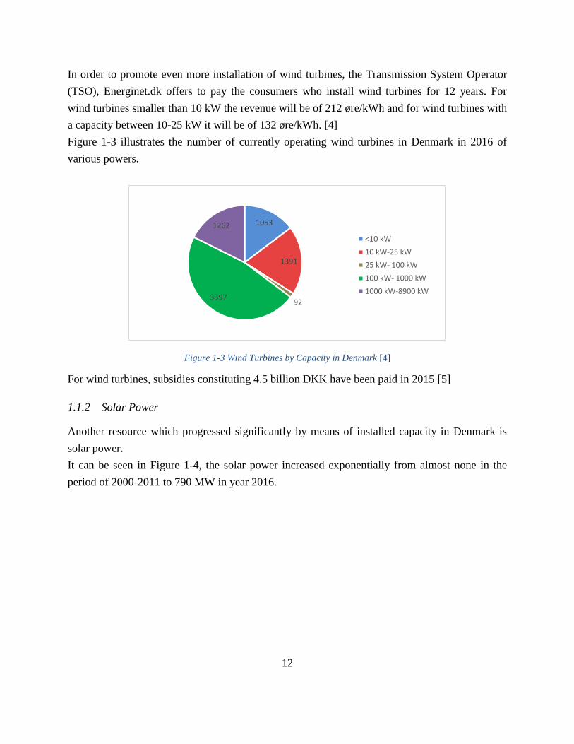
In order to promote even more installation of wind turbines, the Transmission System Operator
(TSO), Energinet.dk offers to pay the consumers who install wind turbines for 12 years. For
wind turbines smaller than 10 kW the revenue will be of 212 øre/kWh and for wind turbines with
a capacity between 10-25 kW it will be of 132 øre/kWh. [4]
Figure 1-3 illustrates the number of currently operating wind turbines in Denmark in 2016 of
various powers.
Figure 1-3 Wind Turbines by Capacity in Denmark [4]
For wind turbines, subsidies constituting 4.5 billion DKK have been paid in 2015 [5]
1.1.2 Solar Power
Another resource which progressed significantly by means of installed capacity in Denmark is
solar power.
It can be seen in Figure 1-4, the solar power increased exponentially from almost none in the
period of 2000-2011 to 790 MW in year 2016.
1053
1391
923397
1262
<10 kW
10 kW-25 kW
25 kW- 100 kW
100 kW- 1000 kW
1000 kW-8900 kW

13
Figure 1-4 Installed Capacity of Photovoltaic Panels in Denmark [3]
According to Energinet.dk, the installed capacity of PVs should reach to 2 115 MW in 2025,
three times larger than the current state, and it is estimated that they will produce 1.950 GWh,
which is equivalent to 5% of the total electricity consumption, making it a resource which should
be analyzed thoroughly. By 2013, the government implemented a new regulation in which it
encourages the installation of PV for net-metering scheme with 60 øre/kWh for first 10 years and
to 40 øre/kWh for the following 10 years.
In Figure 1-5 it is presented the number of currently working PV’s in Denmark under various
powers, with the small panels (under 6kW) being the majority.
Figure 1-5 Number of PVs in Denmark [4]
For solar cells, subsidies constituting 74 million DKK have been paid in 2015 [5]
91407
4300597
<6 kW
6 kW - 50 kW
50 kW - 400 kW

14
As it has been seen previously, wind and solar power are quite expanding at a rapid rate. Having
also the financial support from TSO for the consumers will lead to a change in system, from a
more centralized generation power plants, which are usually based on fossil fuels, to a more
distributed generation power plants based on renewable energy [6].
In this Project, January and July were taken as the months where the studies are done. These
months are representative for the higher consumption in January (Winter case) due to the heating
and lightening, and also high wind speeds. Where, compared to July where there are the periods
of the lowest consumption in the year, together with lower wind speeds, but much more solar
power.
1.1.3 Electric Vehicles
Electric vehicles are based on getting the power from an electric motor instead of a gasoline
engine. These Electric Vehicles can range from electric trains, boats, to electric cars.
By the year of 1830, the first electric vehicles were starting to be used for transportation. They
were considerably different from the electric vehicles known today, mainly because they didn’t
use rechargeable batteries. The first electric vehicles with proper rechargeable batteries, started
to be produced by 1859 [7]. Around 1900, electric vehicles became widely known and used
around the world [8]. However, due to the discoveries made in the oil field, which also took
place at around the same time, making the oil extremely cheap and accessible everywhere, made
the industry to change its attention to gasoline engines [20]. At the end of the 20th century the
electric vehicles regained their popularity due to the fossil fuel shortages, gas emissions and also
transportation regulations.
Compared to the conventional vehicles, EVs have the following advantages [8]
• Energy Efficiency: The conversion of electrical energy from the grid to the wheels is
around 59%-62%, compared to gasoline powered vehicles which can convert up to a
maximum of 17-21% of the energy which is stored in gasoline to the wheels.
• Performance: Electric Motors provide a smooth and quiet operation, with greater
acceleration and also, they require less maintenance compared with the conventional
combustion engines.
• Environmental Factors: Even though conventional gasoline engines have reduced their
emissions in the last years, they are still one important factor in the high percentage of
Greenhouse Gas Emissions generated around the world. On the other hand, EVs have
zero pollutant emissions.

15
• Encouragement Governmental Plans: In order to motivate the public into purchasing an
electric vehicle, and not a conventional one, Governments throughout the world are
supporting economically the people which are buying EVs by lowering the taxes for
them, even by 50%. For example, in Copenhagen, electric cars have free parking places.
[9]
• Solving high wind and solar power penetration: In the periods when there is excess power
from renewable sources, Electric Vehicles can be recharged in order to use the power
efficiently. Furthermore, there can be made an optimization plan with the DSO
(Distribution System Operator) to recharge when it is more suitable economically as well
as safe for the grid.
Even though EVs are rising in popularity at an extreme rate, there are still quite challenges when
buying an EV [10]:
• Driving Range: The range of a normal EV is 100-200 km. Although there are some
models which can reach 300-400 km with a fully charged battery.
• Battery Cost: Depending on the size of the battery, the price is quite high, and throughout
the life of the car, the battery may have to be replaced a couple of times.
• Recharging Times: A full recharge of the battery can take up to 4-8 hours, depending of
the size of the battery.
• Noise Awareness: Although the quiet sound produced by EVs is a plus, regarding the
safety issues it may be a disadvantage.
In Europe, the fuel prices in the last years, have been significantly higher than in North America.
As it can also be seen in Figure 1-6, the costs of owning an EV is lower than owning a
conventional vehicle.

16
Figure 1-6 Comparison of the costs of ownership of EVs compared to Petrol and Diesel Vehicles [10]
With the upcoming popularity of EVs and also because of the national energy policies and
charging infrastructure, the EVs are expected to grow from around 37 000 EVs in 2012 to an
astonishing 669 000 electric vehicles in 2020 according to [11]
Figure 1-7 Expected Future EV share [8]
As shown in Figure 1-7, the EVs will massively increase in the new vehicle market shares,
reaching around 80% of the new vehicles by 2030. This prediction may materialize, according to
[12] which shows companies like Volvo who will stop designing conventional vehicles by 2019.
Furthermore, Mercedes announced that from 2022 it will produce only electric and hybrid
vehicles. Another reason to understand that this trend will arise at an exponential rate is that in

17
2016 Germany’s Bundesrat, which is the federal council, passed a resolution forbidding
conventional vehicles by 2030 [13]
Currently, 20% of the total cars are electric vehicles, according to Figure 1-7. This assumption
will be further utilized in the project.
1.1.4 Heat Pumps
Another type of load to be used in a smart grid, solving the problem of high wind and solar
penetration is heat pump. In 2010, the Danish Energy Association announced that 300 000 heat
pumps will be installed in Denmark by 2025. In Figure 1-8 the cycle of an air-air heat pump is
presented.
Figure 1-8 Heat Pump Cycle [14]
Because of their flexibility potential and their capability to balance the high wind penetration, an
increasing number of research on heat pumps shows the rising interest for this technology in
Denmark [14]. [15]The principle on which a heat pump works is based on the fact that the
electricity needed to provide a certain amount of thermal energy is always lower than the thermal
energy provided, which makes them viable for implementing in homes.
The most common type of heat pump is the air-source heat pump, which transfers heat between
to the house and the outside air. Today's heat pump can reduce the electricity use for heating by

18
approximately 50% compared to the conventional electric resistance heating [30]. For example,
[16]found that if a conventional heater (electrical resistance) is replaced with an air-source heat
pump, the annual savings are around 3000 kWh (6360 DKK). The same heat pump was
compared with an oil system and the savings resulted as 6200 kWh and (13144 DKK). Also
predicts that by 2030 there will be a 40% market penetration for air-air heat pumps. [16]
1.2 Danish Electricity Sector
More than 10 years ago, wind power plants could be disconnected from the grid during
disturbances [7]. However, nowadays it is not possible to do so anymore. Due to the highly
integration of wind power in the power system, new challenges emerge for the system.
In Figure 1-9 it is presented how the generation and consumption affect the voltage in terms of
distance.
Figure 1-9 Challenged in Distribution Grids [7]
Further problems encountered in distribution grids are:
• Voltage rise = Mainly due to fluctuating power;
• Harmonics = Due to an increase of power electronics integrated in the grid;
• Flickers = Due to fluctuating power;
• Unbalances = Due to load demand not being even throughout the day.

19
Considering the above problems, grid codes need to be updated so that they can facilitate a
secure and a reliable system.
Electricity in Denmark sits at a mediocre price comparing to the rest of Europe (including costs
for cleaner energy), but because of the additional taxes, it makes it the highest electricity in
Europe [17]. According to Energinet, the Transmission System Operator, the price for a kWh is
approximately 2.1 DKK [4]. By 2015, the supply security in Denmark was over 99.99% being
one of the highest in the world [18],explaining in some manner why the electricity price is so
high.
The grid limits are presented in Table 1-1. Whereas electric vehicles are significantly heavy
loads reaching up to 11 kW, the voltage dips may be extremely high. Thus, extra-precaution may
be necessary, especially for the peak period (05:00 – 07:00 PM) when the consumers arrive
home and plug-in their EV’s.
Table 1-1 Power Quality Requirements [19]
Parameter Supply Voltage Limit
Frequency LV-MV (50 Hz) ±1%
Voltage Magnitude LV-MV ±10%
Supply Voltage Dips LV 10-50%
MV 10-15%
Short interruptions of supply
voltage LV-MV (up to 3 minutes) 10-900 times per year
Long Interruptions of supply
voltage LV-MV (more than 3 minutes) 48h/year
Harmonics
LV THD≤8% (for each harmonic)
MV THD≤5% (for each harmonic)
1.3 Danish Smart Grid
As previously stated, the electrical consumption is expected to increase in a rapid manner. The
consequences of this change will have an impact on the power quality, on grid losses and also
voltage profiles will be changed considerably. In order to ameliorate these changes, Denmark
when the concept of Smart Grid (Figure 1-10)

20
Figure 1-10 Illustration of the Elements of a Danish Smart Grid [20]
The objective is to make interactions between all the elements. As it can be seen in the figure
above, wind farm, PV panels, electric vehicle, heat pump and the others interact to reduce the
stress in the distribution grids, and also making the prices more economical for the consumers.
Consumers may participate in regulating the market, by charging their EVs in the night when the
electricity prices are lower [20]
Some of the most important concerns that are in a smart grid are:
• Frequency, which can be controlled by matching the generation and the consumption,
assuring that every customer gets the electricity at the same frequency (50 Hz), with
maximum 1% deviation as seen in Table 1-1.
• Voltage, especially voltage dips, which can be controlled by the usage of generators and
transformers, also with special equipment like STATCOMs.
• Current, that has to be maintained between certain levels in order not to exceed the upper
limit of the cables, consequently creating heating problems which translates into losses.

21
1.4 Electricity market in Denmark
Originally, the electricity market, like any other market, is divided into a wholesale market and a
retail market. The main players that participate in trading are the producers, the retailers and the
end users. Nevertheless, the electricity market trading system is more complex, new players such
as, traders and brokers, enter the scene (Figure 1-11) [21]
Figure 1-11 The commercial players and the electricity exchange [21]
Each player has its own role in the electricity market. In the trading process, the electricity is
owned by the player, being able to buy the electricity from a producer and sell it to a retailer or
to buy it from a retailer and sell it to another retailer. The broker acts as an intermediate in the
trading process. For example, a broker may help a retailer to find a suitable producer who will
sell an amount of electricity, at some time. Nord Pool Spot is an example of Nordic electricity
market, which covers countries like Denmark, Norway, Sweden, Finland and Estonia [21]
1.4.1.1 The transmission system operator (TSO)
The role of the TSO is to keep the grid electrically stable in a particular area, keeping the
frequency at 50 Hz and also to make sure that the end users receive the electricity. In Denmark,
the TSO is the state-owned company called Energinet.dk [21]
1.4.2 Regulating power market
When consumption exceeds production, the frequency falls below 50 Hz and it surpasses 50 Hz
in the other situation, therefore the system becomes unstable. As mentioned before, the TSO has
the responsibility to correct these unbalances in the system, by making the producers to increase

22
or decrease the production. These processes are called „up-regulation”, respectively „down-
regulation” [21]
1.4.3 Balancing Power
The electricity market transactions are made hourly. The figure below shows an example where
the electricity is traded for one particular hour, called the hour of operation. The purchase must
be made before the hour of operation.
Figure 1-12 Price setting in the regulating power market [21]
1.4.4 Elspot – Nord Pool Spot’s Day-ahead Auction Market
Elspot market is the Nord Pool Spot’s day-ahead auction market. In this market, the power
purchase orders or sell offers must be sent no later than noon the day before the power is
supplied to the system. The market electricity price for a particular hour is set by intersecting the
purchase curve with the demand curve (Figure 1-13). As both the buyers and the sellers have
submitted orders, the price calculation in this market is called „double auction” .
Figure 1-13 Supply Demand per one day [21]

23
1.5 Project Objectives
The main objective of this project is to conduct a technical analysis regarding the integration of
renewable energy, heat pumps and electric vehicles in a distribution network. The goal is to find
the maximum possible renewable generation for different scenarios of the system, as well as
different control methods. Furthermore, an optimization method is analyzed for different
charging strategies for electric vehicles.
The focus on renewable generation in Denmark is one of the highest in the world and it is
expected to increase even more. Relying this much on renewable generation may cause
improbabilities in generation.
The cold climate of Denmark, as a Nordic country, makes possible the need of heat pumps most
of the year, exception in the summer, where temperature rises towards 20-30 degrees Celsius.
Heat pumps are a great cheap environmental solution, as explained in 1.1.4.
Another solution for a cleaner environment is the electric vehicles, which are gaining
increasingly interest. Electric vehicles not only that are environmental friendly, but they also
help at integrating more renewable power as stated in 1.1.3, mainly due to their sizable load
which depends on the type of vehicle (3-11 kW).
The power variations caused by renewables may sometimes challenge the system. The problems
that may appear are presented in 1.2.
The project aims to identify and solve the problems caused by the high penetration of wind, solar
power, using active and reactive power control, according to the grid codes. Further, an
economic analysis regarding charging strategies of EVs will be analyzed.
In order to do this, the following objectives are considered:
• Modelling of renewable generation (wind and solar) and identify the maximum power
supported by the grid;
• Modelling of the load side (heat pumps and electric vehicles), analyze how will they
affect the system, and determine the new maximum renewable generation that can be
integrated in the system;
• Analyze and compare active power control and reactive power control regarding the
maximum renewable generation;
• Evaluate the impact of different charging strategies for electric vehicles technically as
well as economically.
As mentioned in 1.1, wind and solar power generation are the top two renewable resources in
Denmark, and will continue to be according to the experts’ predictions. For this reason, the two

24
renewable generations are chosen to be studied in this project. On the other hand, due to the high
penetration of renewables, EVs and heat pumps are integrated to balance the grid by consuming
the extra generation. For this analysis to be more accurate, two periods of the year are chosen
due to their differences in wind/solar production, January – high wind, low solar power
production and July – low wind, high solar power production.
With big variations in the power production, it may cause voltage problems, transformer
congestions and line loading problems. The main objective of the project is to determine the
maximum allowable amount of wind power and PV production as well as EVs charging on a
typical distribution grid with the help of active and reactive power control, while respecting all
the problems mentioned previously.
In addition, economic strategies will be made to optimize the energy cost for both aggregators
and consumers, while maintaining stable the operation of the system.
1.6 Methodology
In this master thesis the main program that is used is DigSILENT PowerFactory. With the help
of this program, the steady state analysis is performed. The Newton-Raphson calculation method
is used for load flow simulations. The control and optimization are made by using both Matlab
and DPL, which is the programming language of DigSILENT.
The power curves of heat pumps and wind turbines is calculated in Matlab/Simulink. The
optimization is based on the economical part of different charging schedules for the EVs.
Furthermore, Matlab is used to plot and analyze the output data from DigSILENT.
The described methodology is presented in steps as it follows:
• First, the validation of the IEEE 13 bus is made in order to have a common ground for all
the upcoming scenarios, in winter/summer cases.
• Secondly, the grid is tested to see the maximum allowable wind/solar power it can
support. Moreover, EVs and heat pumps are added to balance the system. Both cases are
economically compared.
• For the charging of EVs, the first case is considered dumb charging (charging as soon as
the consumer arrives home). To be a realistic case, the household consumption of Danish
houses, the driving patterns and the available charging times are analyzed.
• Active and reactive power control of the system just for the WT, due to the bigger impact
of wind speed in Denmark, and they are performed according to the grid codes.

25
• Furthermore, a smart charging strategy of the electric vehicles, the improvement of the
system is analyzed from a technical and economical point of view.
1.7 Limitations
The limitations encountered in this project are:
• In this project, the study is limited to a relatively small residential distribution grid, and
for this reason the wind speed and solar irradiation are considered equal for all wind
turbines and solar photovoltaic panels.
• The load profiles are taken for one day in January, representing a higher base household
consumption with more wind and lesser solar power, and one day in July, with slightly
lower base household consumption, and with more solar power and lesser wind power
generation.
• The wind turbines and photovoltaic panels are modelled as only active power generators
(power factor of 1), except the reactive power control which will have variable power
factor for the wind turbines. The heat pumps are modelled as loads with a power factor of
0.97, and the households are modelled with a power factor of 0.95. No heavy industry
which would have a lower power factor is represented in this simulation.
• The study is performed on IEEE 13 bus network and not on a real network, and it is
simulated with the fundamental frequency of 50 Hz (study is made for Denmark),
different to the original model which is modelled with 60 Hz, as the model originates
from America.
• The problems regarding the grid, such as voltage dips, flickering, harmonics are not
considered.
• The analysis of heat pump integration is studied only in January case due to temperatures,
in July being more or equal to the desired temperature (household temperature) which in
this project is set to 20° C.
• The control methods are conducted with regards to the wind turbine power only.
1.8 Outline of the thesis
Chapter 1 – Introduction-In this chapter the background, project objectives, methodology of
project, and project limitations, are studied for various components of the system.
Chapter 2 – Description of the distribution system – In order for the simulation to be as correct as
possible, the need of validation occurs. In this chapter the validation of the IEEE 13 Bus
Network is presented.

26
Chapter 3- Renewable Generation- For the simulation to be accurately performed, the profiles of
each component should be accurately modelled. In this chapter the WT, PV , HP, EV are being
modelled.
Chapter 4 – Maximum Allowable Renewable Integration with and without Heat Pump
Integration. Having the validation completed, the study of the maximum renewable integration is
performed. The impact of heat pumps is also analyzed with regards to the increase of renewable
generation.
Chapter 5 – Control Schemes- In this chapter, the maximum renewable generation, discovered in
chapter 4, is increased even more by performing active and reactive power control.
Chapter 6 – Economical Analysis- This chapter consists, of the techno-economic analysis, of
different charging methods. The profits for the EV owners is determined, for both January and
July.
Chapter 7- Conclusions and Future Work – In this chapter the conclusions determined by
performing this analysis are shown. Further, future improvements to the study are shown.

27
2 Description and validation of the system
In this section, the IEEE 13 bus distribution system is presented and validated. Firstly, the
process of power flow analysis is described, followed by the system description and finally, the
validation of the model.
2.1 Power Flow Analysis
The power system flow analysis is a computational procedure which uses numerical algorithms
to determine the steady state operating characteristics of a power system network from the given
line and bus data [22]
As shown in Figure 2-1, the input for the load flow, consists of the line data and bus data the
magnitude of bus voltage (|V|), and the angle of bus voltage referred to a common reference (δ)
[22]
Figure 2-1 Load Flow Parameters
This method is used in power systems (transmission and distribution) in order to have a fast
analysis of the current state of the system. The speed of the steady state analysis is highly
important, some simplified component models are used, as shown in Table 2-1.
Table 2-1 Simplified Models for Electrical Equipment [19]
Equipment Simplified Model
Short Lines (below 80 km) Series Impedance
Medium and Long Lines (above 80 km) π model
Transformer Series Reactance
Loads Constant Power
Generators Constant power source operating at a fixed
voltage
In Figure 2-2 the transmission line model (𝜋 model) is presented. It is modelled on the bases of
the 𝜋 model, where R + jX is the line impedance, and Y/2 is the half line charging admittance.

28
Figure 2-2 Transmission Line Model
In each load flow study, the type of each bus bar is divided in three types. Each of these types is
different, each having its role into performing the load flow analysis.
In each power flow study, there are three types of buses, which are determined by the known and
unknown variables. Depending on which components are present in the system and on the
known variables, the type of bus can be determined.
2.1.1 Voltage Controlled Bus
The model of the PV bus or Voltage controlled bus, where the generation is connected, is
presented in Figure 2-3. The value of the voltage magnitude is maintained at a constant level for
as long as the reactive power is maintained between the limits (Qmin < Qrequired< Qmax). If the
reactive power gets over the limits, the bus becomes a load bus (PQ bus) with the Q limit that has
been breached, as the new reactive power for the bus. Equation (1) describes the total generation
power at node “I”. [22]
Figure 2-3 PV Bus
Gi Gi GiS P jQ (1)

29
2.1.2 PQ Bus (Load Bus)
The model of PQ bus, also known as a load bus, is depicted in Figure 2-4. In a power system this
type of buses represent 85% of the total number of nodes. The total power demand is presented
in equation 2 [22]
Figure 2-4 Load Bus Model
Di Di DiS P jQ (2)
2.1.3 Slack Bus
The slack bus, also known as the reference bus, is limited to just one in every system. The phase
angles of all the other buses are relative to the slack bus angle. In real life, the slack bus doesn’t
exist, it is used just for simulations. All the losses in the system that are not supported by other
types of generators are supported by the slack bus.. Another important feature is that the slack
bus has to adjust the power to hold the voltage constant [22]
Table 2-2 Bus Types Specified vs Unspecified parameters presents the specified and unknown
variables for the load flow for all 3 types of buses.
Table 2-2 Bus Types Specified vs Unspecified parameters [22]
Bus Type Specified Variables Unknown Variables
PQ P, Q |V|, δ
PV Bus P,|V| Q, δ
Slack Bus |V|, δ P, Q
2.1.4 The Bus Admittance Matrix

30
The bus admittance matrix or the node admittance matrix is used in energy engineering to
describe a power system with N buses, which is a square matrix composed of N by N elements.
This matrix is used to calculate all the parameters necessary such as voltages or angles for each
node [50].
In Figure 2-5 it is presented a simple 4-bus network with 2 generation nodes and a transformer.
Figure 2-5 Simple 4 Bus Network
Considering the 4-bus network, it can be easily understood how the unknown variables can be
represented, knowing just two variables for each bus, using Table 2-2 [22]
Figure 2-6 Simple 4 Bus Network with variables [19]
Moreover, the normal network presented in Figure 2-5 needs to be transformed into a bus
admittance diagram. In Figure 2-7, it is presented the bus admittance diagram of the system
represented in Figure 2-5.

31
Figure 2-7 Bus Admittance Diagram
Further, the admittance elements yij are calculated for each point of the diagram. The formula is
presented in equation 3:
1 1
ij
ij ij ij
yZ R jX
(3)
Where, yij [IΩ-1I] is the admittance between nodes i and j; zij is the impedance from node i and j;
rij [Ω] is the resistance part, and xij [Ω] is the reactance between nodes i and j.
After the admittances for all the buses (yij, yii) have been calculated, the next step is to calculate
the mutual admittances, that will be used to build the admittance matrix. The equation is
presented in (3):
ij ijY y (3)
Furthermore, the self-admittance elements for each node must be calculated. They are equal to
the sum of admittances connected to that particular node. The position for each element will be
on the diagonal axis of the bus admittance matrix, and it can be calculated using equation (5):
1
N
ii i j innn i
Y y y
(4)
After all the necessary elements have been calculated, the admittance matrix can be built. For the
system presented in Figure 2-6, the admittance matrix is shown below:
11 12 13 14
21 22 23 24
31 32 33 34
41 42 43 44
nn
Y Y Y Y
Y Y Y YY
Y Y Y Y
Y Y Y Y
(5)

32
One big advantage of the Ybus is that it has symmetric elements along the diagonal axis, meaning
that Y12=Y21, Y13=Y31 and so on. Furthermore, in a power system not all the nodes are connected
together, making the bus admittance matrix a sparse matrix with many elements being 0. This
reduces significantly the computational time and the required storage [23]
As shown in Table 2-2 Bus Types Specified vs Unspecified parameters [22], there are different
types of buses, with different specified variables and unknown variables. By knowing what type
of bus is, there can be calculated the active and reactive power of the node, with the help of
power flow equations shown below:
N
k k j kj k j kj k jj=1
P = V V G cos(θ -θ )+B sin(θ -θ ) (6)
Q N
k k j kj k j kj k jj=1
= V V G sin(θ -θ )+B cos(θ -θ ) (7)
Where:
Pk=active power at node k; Qk=reactive power at node k; Vk=voltage at node k; Vj=voltage at
node j; Gkj=real component of the element in the admittance matrix between node k and j;
Bkj=imaginary component of the element in the admittance matrix between node k and j;
θk=voltage angle at node k; θj=voltage angle at node j.
For simple system networks, the power flow can be done manually using equations 7 and 8. For
more complex network systems, iterative methods are used.
The most important methods are:
• Gauss-Siedel Method (G-S);
• Newton-Raphson Method (N-R);
• Fast Decoupled Method (FDLF).
A comparison between the three methods, where criteria such as system size, storage and more is
presented in Table 2-3.

33
Table 2-3 Comparison between load flow methods.[24]
G-S N-R FDLF
System size Smaller Unlimited Unlimited
Storage Minimal Large 40% of N-R
Programming Easy Complex Less complex
Convergence Worst Best Good
Accuracy Less Most Good
As it can be seen in the table above, Newton-Raphson convergence method has the best results.
The only disadvantage is that the programming is complex. In Simulation programs such as
DigSILENT PowerFactory, the Newton-Raphson method is used.
2.2 IEEE 13 bus distribution system validation
The validation of the IEEE 13 bus network system is needed in order to create a benchmark
model of the distribution grid for the simulations which are performed on it. After the validation
is performed, renewables, electric vehicles and heat pumps are added, and the system is tested,
different scenarios and scenarios. In Figure 2-8, the IEEE 13 Bus test network is presented.[25]
Figure 2-8 IEEE 13 Bus Test Network [25]
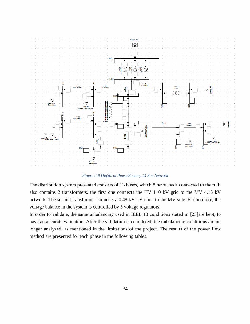
The distribution model [54], shown above, is modeled using DigSILENT Powerfactory, and it is
presented in Figure 2-9 including just the base model, where the validation is performed.
34
Figure 2-9 DigSilent PowerFactory 13 Bus Network
The distribution system presented consists of 13 buses, which 8 have loads connected to them. It
also contains 2 transformers, the first one connects the HV 110 kV grid to the MV 4.16 kV
network. The second transformer connects a 0.48 kV LV node to the MV side. Furthermore, the
voltage balance in the system is controlled by 3 voltage regulators.
In order to validate, the same unbalancing used in IEEE 13 conditions stated in [25]are kept, to
have an accurate validation. After the validation is completed, the unbalancing conditions are no
longer analyzed, as mentioned in the limitations of the project. The results of the power flow
method are presented for each phase in the following tables.

35
Table 2-4 Voltage and Power Profiles for Phase A
NODE Sim VA
(p.u.)
IEEE
VA
(p.u.)
Diff
(%)
Sim PA
(kW)
IEEE PA
(kW)
Diff
(%)
Sim QA
(kVAr)
IEEE
QA
(kVAr)
Diff
(%)
RG60 1.05 1.05 0 - - - - - -
632 1.0413 1.042 0.067 - - - - - -
645 1.0317 1.0329 0.116 - - - - - -
646 1.03 1.0311 0.1 - - - - - -
633 1.0392 1.041 0.17 - - - - - -
634 1.02 1.0218 0.176 160 160 0 110 110 0
671 1.0531 1.0529 0.1 390 385 1.3 219.3 220 0.4
684 - - - - - - - - -
611 - - - - - - - - -
692 1.0531 1.0529 0.1 - - - - - -
675 1.0551 1.0553 0.018 470 485 3.1 190 190 0
680 1.0531 1.0529 0.1 - - - - - -
652 - - - 120 123.56 2.9 80 83.02 3.7
Table 2-5 Voltage and Power Profiles for Phase B
NODE Sim VB
(p.u.)
IEE VB
(p.u.)
Diff
(%)
Sim PB
(kW)
IEE PB
(kW)
Diff
(%)
Sim QB
(kVAr)
IEEE
QB
(kVAr)
Diff
(%)
RG60 1.05 1.05 0 - - - - -
632 1.0413 1.042 0.067 - - - - - -
645 1.0317 1.0329 0.116 175.6 170 - 130 125 -
646 1.03 1.0311 0.1 242.1 240.66 - 136.5 138.12 -
633 1.0392 1.041 0.17 - - - - - -
634 1.02 1.0218 0.176 120 120 0 90 90 0
671 1.0531 1.0529 0.1 405.1 385 5.1 218 220 0.2
684 - - - - - - - - -
611 - - - - - - - - -

36
692 1.0531 1.0529 0.1 - - - - - -
675 1.0551 1.0553 0.018 73.2 68 3.1 68 60 3.8
680 1.0531 1.0529 0.1 - - - - - -
652 - - - - - - - - -
Table 2-6 Voltage and Power Profile for Phase C
NODE Sim VC
(p.u.)
IEEE
VC
(p.u.)
Diff
(%)
Sim PC
(kW)
IEEE PC
(kW)
Diff
(%)
Sim QC
(kVAr)
IEEE
QC
(kVAr)
Diff
(%)
RG60 1.05 1.05 0 - - - - - -
632 1.0413 1.042 0.067 - - - - - -
645 1.0317 1.0329 0.116 - - - - - -
646 1.03 1.0311 0.1 - - - - - -
633 1.0392 1.041 0.17 - - - - - -
634 1.02 1.0218 0.176 120 120 0 90 90 0
671 1.0531 1.0529 0.1 370 385 3.9 220 220 0
684 - - - - - - - - -
611 - - - 160 165.54 3.4 74.3 77.9 4.6
692 1.0531 1.0529 0.1 171.3 168.37 1.71 146.9 149.55 1.77
675 1.0551 1.0553 0.018 270 290 5.89 200 212 5.6
680 1.0531 1.0529 0.1 - - - - - -
652 - - - - - - - - -
2.3 Summary
After analyzing the tables mentioned above, it can be concluded that the highest differences are
for phase C for node 675. Here for active and reactive power the difference is 5.89 % and 5.6 %,
respectively. The difference for the reactive power can be explained by mentioning that the IEEE
13 bus network originates from America, where the nominal frequency is 60 Hz, not valid in
Europe. The simulations of the model with 50 Hz changes the reactance, as well as the reactive
power.

37
Because all the results are close to/below the 5% difference margin, it can be concluded that the
model is validated with respect to the IEEE 13 bus network model [52]. Therefore, the validated
model will be used for further investigations where maximum renewable energy is tested in
combination with electric vehicles and heat pumps. For the upcoming simulations, the voltage
regulators (phase A, phase B, phase C) are replaced by a 3-phase transformer since there will be
no more unbalances in the loads, everything being 3-phase.

38
3 Modelling of the generation and consumption profiles
As shown in List of Figures
Figure 1-1 Installed RE Capacity in Europe [MW] 2000-20016 [3] ............................................ 11
Figure 1-2 Installed Wind Capacity in Denmark [3] .................................................................... 11
Figure 1-3 Wind Turbines by Capacity in Denmark [4] ............................................................... 12
Figure 1-4 Installed Capacity of Photovoltaic Panels in Denmark [3] ......................................... 13
Figure 1-5 Number of PVs in Denmark [4] .................................................................................. 13
Figure 1-6 Comparison of the costs of ownership of EVs compared to Petrol and Diesel Vehicles
[10] ................................................................................................................................................ 16
Figure 1-7 Expected Future EV share [8] ..................................................................................... 16
Figure 1-8 Heat Pump Cycle [14] ................................................................................................. 17
Figure 1-9 Challenged in Distribution Grids [7]........................................................................... 18
Figure 1-10 Illustration of the Elements of a Danish Smart Grid [20] ......................................... 20
Figure 1-11 The commercial players and the electricity exchange [21] ....................................... 21
Figure 1-12 Price setting in the regulating power market [21] ..................................................... 22
Figure 1-13 Supply Demand per one day [21].............................................................................. 22
Figure 2-1 Load Flow Parameters................................................................................................. 27
Figure 2-2 Transmission Line Model ........................................................................................... 28
Figure 2-3 PV Bus ........................................................................................................................ 28
Figure 2-4 Load Bus Model .......................................................................................................... 29
Figure 2-5 Simple 4 Bus Network ................................................................................................ 30
Figure 2-6 Simple 4 Bus Network with variables [19] ................................................................. 30
Figure 2-7 Bus Admittance Diagram ............................................................................................ 31
Figure 2-8 IEEE 13 Bus Test Network [25] ................................................................................. 33
Figure 2-9 DigSilent PowerFactory 13 Bus Network .................................................................... 34
Figure 3-1 Wind power generation and household electricity consumption for January and July41
Figure 3-2 Wind Speed vs Power Curve for Osiris 10 turbine ..................................................... 42
Figure 3-3 Wind Speed and Wind Power Generation for 1 day in January/July .......................... 43
Figure 3-4 PV Power Generation July and January ...................................................................... 47
Figure 3-5 The Lift [59] ................................................................................................................ 48
Figure 3-6 COP vs Lift [30] .......................................................................................................... 48
Figure 3-7 Thermal Energy vs Electrical Energy ................................................................................ 49
Figure 3-8 Average daily driving distance in DK [32] ................................................................. 50

39
Figure 4-1 The Critical Components of the system ...................................................................... 53
Figure 4-2 Household Electricity Consumption January/July 2013 .................................................. 55
Figure 4-3 Max Renewable Cases 1-4 January............................................................................. 57
Figure 4-4 Node 675 Voltage Levels January .............................................................................. 58
Figure 4-5 Transformer Loading January ..................................................................................... 58
Figure 4-6Line Loading January Case .......................................................................................... 59
Figure 4-7 Max Renewable Generation (WT+PV) January ......................................................... 60
Figure 4-8 Maximum Renewable integration July ....................................................................... 61
Figure 4-9 Transformer Loading in July ....................................................................................... 62
Figure 4-10 Node 675 Voltage in July .......................................................................................... 63
Figure 4-11 Lines Loading July .................................................................................................... 64
Figure 4-12 Renewable Maximum Generation July ..................................................................... 64
Figure 4-13 New Maximum Renewable Generation January ....................................................... 65
Figure 4-14 Old vs New Generation January ............................................................................... 66
Figure 5-1 Active Power Control Flowchart ................................................................................. 69
Figure 5-2 Max WT January ......................................................................................................... 70
Figure 5-3 Voltage, Transformer and Line profiles for 85o WTs (January) ................................ 71
Figure 5-4 Max WT July (600 WTs) ............................................................................................. 72
Figure 5-5 Voltage, Transformer and Main Line profiles for 600 WTs (July) .............................. 73
Figure 5-6 Reactive Power Control profiles (January) ................................................................. 75
Figure 5-7 Reactive Power Control (July) ............................................................................................ 76
Figure 6-1 Simulation Method of EV Charging ........................................................................... 79
Figure 6-2 Dumb Charging January ............................................................................................. 81
Figure 6-3 Loading difference between the Main and Second Transformer ................................ 82
Figure 6-4 Smart Charging Profiles .............................................................................................. 84
Figure 6-5 Dumb charging profiles- July ...................................................................................... 86

40
Summary
Renewable Generation such as Wind Power Generation as well as Solar Power Generation, is on
a continual rise. Relying this much on renewable integration, may stress the system, and also
generate unbalances in the system. Methods to store the extra energy when the production is
bigger than consumption (especially in the night). Loads such as Electric Vehicles and Heat
Pumps.
In this master thesis, the renewable integration is modelled and raised to the maximum capability
that the system can support, regarding its limits. The system is modelled and validated on the
IEEE 13 Bus Network. Furthermore, Heat pumps are integrated as well into the system, in order
to increase the consumption, during the off-peak household consumption hours. After the
integration of heat pumps, the number of wind turbines possible to operate in the system,
increases by 10 times.
Control Methods are further analyzed, to increase even more the renewable generation that can
be integrated into the system. Active Power Control consists of lowering the power production in
the periods where the system limits may be violated.
Another type of control, analyzed in this project, is the reactive power control, based on
generating or consuming reactive power in order to keep the system in its established limits. By
doing this method, the maximum number of Wind Turbines and PV panels are found.
Finally, different charging strategies are studied, in order to find the highest profit for the EV
owners, while keeping the system under the limits.
Introduction, the number of PV installments in Denmark has abruptly increased over the last
years and it will continue to rise. Furthermore, wind turbines are widely used due to the high
winds available here.
In this chapter, the solar, wind, heat pumps and EVs power curves are presented by showing the
models which were used to determine the generated (WT and PV) or consumed (EV and HP)
power.

41
For this project, the data used to calculate the renewable generation power curves (WT+PV) is
based on [26], recorded in Aalborg, Denmark, for one year, from 01/01/2013 - 31/12/2013.
Two periods of the year, January and July, have been considered for further studies. These
months are representative for the higher consumption in January (Winter case) due to the heating
and lightening, and also high wind speeds. On the other hand, July has periods with the lowest
consumption in the year and lower wind speeds, but much more solar power. Furthermore, as the
wind is the most important renewable energy source in Denmark, a 2-week (17-01-2013 to 31-
01-2013 and 17-07-2013 to 31-07-2013) visualization profile is conducted in Figure 3-1 in order
to better understand the behavior of both wind production and consumption, for both periods. In
the figure below, it can be seen that on average, the wind power production is higher in January,
compared to July. For further analysis, 28-01-2013 and 26-07-2013 have been chosen, as their
wind power profiles are neither too low or too high.
Figure 3-1 Wind power generation and household electricity consumption for January and July
3.1 Wind Turbines Power Simulation
For the wind turbine generation case, the power is determined using a look-up table in
Matlab/Simulink, where the input is the wind speed and the output is the power generated. The
lookup table consists of a Wind vs Power curve (v-P) for the Osiris 10, 10 kW wind turbine. This
turbine is accepted in the Danish Market, according to [27]The control of the power is done with
the help of the active and passive pitch control [27]Some important specifications of the turbine
are shown below in Table 3-1.

42
Table 3-1 Osiris 10 Wind Turbine Specifications [28]
Specifications Values
Rated Power 10 kW
Cut in Wind Speed 2.5 m/s
Cut out Wind Speed 22 m/s
Rated Wind Speed 9.5 m/s
Passive Power Regulation Pitch angle adjustment
Blade Diameter 9.7 m
Furthermore, the wind speed – power curve used in the look-up table is shown in Wind Speed vs
Power Curve for Osiris 10 turbine.
Figure 3-2 Wind Speed vs Power Curve for Osiris 10 turbine
In Figure 3-3, the wind speed for a day in January and a day in July, as well as the power
generated by one wind turbine with the wind speed, are presented. During winter the wind is
more significant throughout the day, than during the night. Consequently, the power of the wind
turbines provided will be as well higher. For July, the power is almost zero until 12 AM, due to
the restriction of the turbine cut-in wind speed.

43
Figure 3-3 Wind Speed and Wind Power Generation for 1 day in January/July
3.2 Photovoltaic Panels Power Simulation
The PV system comprises 6 panels, with a rated power of 225 W each panel, resulting a total
rated a power of 1350 W.
For the Power Curve Simulation of the PV panels the following parameters were taken from
[26]:
• Global Horizontal Irradiance (G)
• Diffused Horizontal Irradiance (Gd)
• Solar Azimuth Angle (AZ)
• Air Temperature (Ta)
Considering 4 parameters instead of one, as in the case of Wind Power Simulation subchapter, a
more thorough calculation is needed to perform in order to accurately calculate the power curve.
Furthermore, taking into consideration these parameters, one can find the output power of the PV
in three steps. Firstly, the total tilted irradiance is calculated, using the Perez irradiance model
[4]. This is done with respect to the tilted angle of the PVs used in Denmark, which is 42o [2].
Secondly, The PV cell temperature is calculated, because the output power is dependent on the
air temperature. The air temperature is desired to be as low as possible for a better efficiency of
the PV panel. Finally, the PV power is calculated, with respect to the area of the PV panels,
which in this case were taken to be 4 PV panels summing up an area of 6.4 m2.

44
3.2.1 Total tilted irradiance calculation
The total tilted irradiance (𝐺𝑡𝑜𝑡𝑎𝑙−𝑡𝑖𝑙𝑡𝑒𝑑) has been calculated for one year from the provided data
using the Perez irradiance model. To calculate 𝐺𝑡𝑜𝑡𝑎𝑙−𝑡𝑖𝑙𝑡𝑒𝑑 the following calculations have been
conducted.
The direct horizontal irradiance (𝐺𝑏) is calculated using the equation below:
b dG G G (8)
The zenith angle (ZA) and the incidence angle (IA) are calculated using the following equations:
90ZA SA (9)
where SA is the solar altitude angle in degrees.
arccos[cos( ) cos( ) sin( ) cos( )]IA ZA AZ (10)
where AZ is the solar azimuth angle, in degrees, and is the tilt angle, considered 42 for
Denmark, according to [5].
Further, the day angle (B), in radians, is calculated:
2 ( 1)
365
dnB
(11)
where dn is the day number, for one year. And for this simulation dn=208 (July) and dn=28
(January).
The eccentricity correction factor of the earth’s orbit (𝐸0) using the day angle (B) value for each
day, is calculated:
0 1 0.034cos( ) 0.001sin( ) 0.0007cos(2 ) 0.00007sin(2 )E B B B B (12)
Next, 𝐸0 is used to calculate the extraterrestrial irradiance on horizontal surface (𝐺𝑜𝑛):
0on scG G E (13)
where 𝐺𝑠𝑐 = 1367 𝑊/𝑚2.
The relative optical air mass (m) is calculated below:
1.253 1[sin( ) 0.15( 3.885) ]m SA SA (14)
where SA is in degrees.

45
Further, the sky clearness () is calculated:
3
3
( )
( 1.041 )
(1 1.041 )
d b
d
G G
G ZA
ZA
(15)
where ZA is the zenith angle measured in radians, this time.
The irradiance coefficients are obtained from the table below, based on the value of .
Table 3-2 Irradiance Coefficients with respect to the Sky Clearness
F11 F12 F13 F21 F22 F23
1 -0.008 0.588 -0.062 -0.060 0.072 -0.022
2 0.130 0.683 -0.151 -0.019 0.066 -0.029
3 0.330 0.487 -0.221 0.055 -0.064 -0.026
4 0.568 0.187 -0.295 0.109 -0.152 -0.014
5 0.873 -0.392 -0.362 0.226 -0.462 0.001
6 1.132 -1.237 -0.412 0.288 -0.823 0.056
7 1.060 -1.600 -0.359 0.264 -1.127 0.131
8 0.678 -0.327 -0.250 0.156 -1.377 0.251
Using the irradiance coefficients from the table above, the circumsolar ( 𝐹1 ) and horizon
brightening coefficients (𝐹2) are calculated:
1 11 11 13F F F F Z (16)
2 21 22 23F F F F Z (17)
Where () is the sky’s brightness and it can be calculated using the equation below:
d
G m
G
(18)
Further, the beam, tilted irradiance and the reflected irradiance are calculated:
( )b b
aG G
b (19)
1 1 2
(1 cos( ))( ) (1 ) sin( )
2d d
aG G F F F
b
(20)

46
where: 𝑎 = max(0, cos(𝐼𝐴)) 𝑎𝑛𝑑 𝑏 = max (0.087, cos(𝑍𝐴))
(1 cos( ))
( )2
rG G pg
(21)
where: =42 and pg=0.2.
Finally, 𝐺𝑡𝑜𝑡𝑎𝑙−𝑡𝑖𝑙𝑡𝑒𝑑 is given by equation:
( ) ( ) ( )total tilted b d rG G G G (22)
3.2.2 PV cell temperature calculation
The total tilted irradiance, calculated before, is now used to calculate the temperature of the PV:
20
800c air total tilted
NOCTT T G
(23)
where NOCT is the normal operating cell temperature and it is considered 45.
PV output power calculation
Finally, the PV output power is calculated following the next steps:
[1 ( 25 )]pv ref T ck T (24)
where ηref =0.15 is the reference solar cell efficiency and kT=0.004 is the temperature coefficient.
pv pv total tiltedP G A (25)
where A is the PV module area, expressed in m2.
Finally, the power can be seen in Figure 3-4, shown below, for a day in July and one in January.
As expected, the power generated in July is bigger than the one generated in January, due to
more irradiance being available in July.

47
Figure 3-4 PV Power Generation July and January
3.3 Heat Pump Power Demand
As mentioned in chapter 1, heat pumps can act as a load, helping the system by storing the
excess power. In this project the air-air heat pumps will be used as being the most common in
Denmark.
Heat pumps efficiency is greatly depending on the operating temperatures. These temperatures
are the outside temperature, called ‘source temperature’ (environmental temperature), from
where the air is extracted. The temperature where the air is delivered is called ‘sink temperature’.
The difference between the source temperature and the sink temperature is also known as ‘lift’.
The smaller the lift is, the bigger the efficiency, due to the lesser energy needed to reach the
desired temperature. For example, the energy needed to heat an apartment at 20 °C with the
outside temperature of 2 °C, will be smaller than the energy needed to heat the apartment at the
same temperature, with the outside temperature being -10 °C. [29]
In Figure 3-5 a better representation of the lift is presented, from an outside temperature of -20
°C to a desired temperature of 20°C.

48
Figure 3-5 The Lift [59]
Heat Pumps heating efficiency can be expressed with the help of the performance coefficient
(COP). For heating purposes, COP can be expressed as the heat energy delivered by the heat
pump divided by the energy needed from the pump, compressor, and the fan [29]
heating
UsefulHeatingEnergyCOP
CompressorEnergy FanEnergy PumpEnergy
(26)
Since the energy required by the heat pump (compressor, fan and pump) is less than the actual
useful thermal energy provided by the heat pump, this coefficient (COP) will be always bigger
than 1. For example, for a COP equal to 3, excluding the energy drawn from the environment
calculations, a heat pump can provide 3 kWh thermal energy for heating with just 1 kWh
electrical energy [29]
Figure 3-6 COP vs Lift [30]
In Figure 3-6, a graphical relation between COP and Lift is presented for different types of heat
pumps. In this project, the most common Standard Air Sourced Heat Pump is utilized, which is
the heat pump with the lowest COP [30]
Finally, in Figure 3-7 the electrical energy needed for one day in January for an air-air heat
pump is shown. Between 00:00 -06:00 A.M., where the outside temperature is lower, it is seen
that the thermal power provided is big in order to keep the temperature constant at 20 °C.
Following the period of 12:00 to 06:00 P.M. no power is required due to the inside temperature
keeping constant at the set temperature (20°C).

49
Figure 3-7 Thermal Energy vs Electrical Energy
According to the Danish Energy Agency [31] in 2014 the percentage of heating for Denmark just
from heat pumps was approximately 12%. Since heat pump installations are on a continuing rise
as stated in chapter 1, the percentage of heat pumps in the current project is set to 12%.
3.4 Electric Vehicle Integration
To accurately integrate electric vehicles into the simulation, some important parameters have to
be taken in consideration, such as: percentage of EVs of the total vehicles, charging profiles,
arriving times of EVs, consumption/km, distances travelled.
For the parameters, three data sources will be used in this project [30]
• MDCars (Database of Odometer readings);
• TU Data (Danish National Transport Survey);
• AKTA Data (GPS-Based Data that Follows the Vehicles).
These sources analyze the behavior of the EV owners and record the data in order to better
predict certain aspects in the future.
3.4.1 Number of EVs

50
As presented in section Electric Vehiclesthe estimated number of EVs in Denmark is 20% of the
total vehicles. For this project, it is assumed that for all houses (6405 total) 20% of them have an
electric vehicle.
3.4.2 Driving Distance
The average driving distance for each day of the week is presented in Figure 3-8 The highest
distance travelled is 55 km in a Friday. For this project, the overall distance is taken as the
average distance of all days, 48 km [32]
Figure 3-8 Average daily driving distance in DK [32]
3.4.3 Charging power levels
The duration of the EV charging is determined by the charger power level. There are 3 types of
charging levels, depending on the power, as well as, where or how the EV is going to be charged.
According to [33]the EV owners prefer the second charging level as it takes less charging time of
the vehicle. Furthermore, the charging level 2 is chosen for this study with 11 kW power
capability of charging, according to [33]. This high level of power can be achieved because most
of the Danish houses have 3-phase electrical installation.

51
Table 3-3Charging Power Level[34]
Level Charger
location
Typical use Energy
supply
interface
Power level
Level 1
(Opportunity,
120V/230V)
On-board
1-phase
Home or
office
Convenience
outlet
Up to 2 kW
Level 2
(Primary,
240V/400V)
On-board
1 or 3 phases
Dedicated
outlets
Dedicated
outlet
4-20 kW
Level 3 (Fast,
480V/600V
or direct DC)
Off-board
3-phase
Commercial
filling station
Dedicated
EVSE
50-100 kW
3.4.4 Charging Profiles
Regarding the charging profiles, for this project two profiles have been chosen. One of them is
called ‘Dumb Charging’, where the owner comes home and starts charging the EV immediately
and the other one is called ‘Smart Charging’ or ‘Controlled Charging’, where with the help of the
DSO the EVs charge during the night, lowering the stress on the system, as well as providing
economical profit, due to charging at a cheaper price electricity hour.
3.4.5 Consumption needed for EVs
According to [32] the average consumption of a normal electric vehicle ranges between 0.12
kWh/km and 0.22 kWh/km. For this thesis, the energy needed for one EV is considered 0.22
kWh/km. From this and from the average distance found earlier in subchapter 3.4.2, the average
energy needed for each EV in one day can be calculated as:
0.22 / 48E kWh km km (27)
From the above equation it can be concluded that the average energy needed for each EV is
approximately 11 kWh.

52
3.5 Summary
This chapter focus is the description of the generation and load part used in this master thesis.
Different methods are used in modelling these parts in order to have a high accuracy. The input
data, such as wind speed or solar irradiance, give the power curves of the generation, as well as
from the measured thermal output power of the heat pump and the electricity consumed, the
efficiency can be calculated. This project is focusing mostly on the system behavior, meaning
that most of the EV parameters presented above were taken as average values.

53
4 Maximum Allowable Renewable Integration with and without Heat Pump
Integration
In this section, the maximum allowable renewable integration must be found. In order to do this,
the voltage and transformer/line loadings must be kept between the established boundaries.
Figure 4-1 The Critical Components of the system
The system limits of the main components shown in the figure above are presented below:
• Voltage limit – this voltage limit consists of the limit set between 0.95 and 1.05 p.u. For
this limit, the Node 675 will be analyzed. This node is chosen in particular as it is seen
later in Figure 4-3, that this is the weakest node. This is required in order to see the
fluctuations of the voltage (measured in p.u.).
• Main Line Loading – to not overload the lines and cause heating problems, this limit
should not exceed 100%.
• Main Transformer Loading- (HV side 115-4.16 kV LV side) presented in Figure 4-1, the
main transformer is shown. This is required to see the loading factor of the transformer in
the different scenarios investigated (measured in %). The transformers loading limit

54
should be kept under 100%, in order to not cause problems such as gassing of the
transformer.
• Second Transformer Loading- (HV side 4.16 – 0.48 kV LV side) Same as above, the
loading factor will be studied for this case.
To find this value, the generation is increased for one day until one of the limits specified in
chapter 1 is violated, or decreased if the limits are already violated, until the upper critical limit
is reached. This procedure is conducted for two different seasons, January and July. These
seasons are chosen due to their difference in load consumption throughout a day.
4.1 Household consumption
Initially, the base household consumption for January and July is present. The consumption in
normal houses depends directly on the number of persons living in the house. Therefore, the
consumption data is taken from with three different profiles, low, medium and high. Further,
there are presented the number of persons for each category, as well as the percentage of the final
consumption they represent, according to [35]
• Low Consumption = One Person (30% of final consumption)
• Medium Consumption = Male + Female + one children (51% of final consumption)
• High Consumption = Male + Female + three children (19%of final consumption)
Furthermore, in Figure 4-2 the curves are presented, with the averaged curve being the one
which will be used further in this project for January and July, respectively.

55
Figure 4-2 Household Electricity Consumption January/July 2013
Moreover, the number of houses at each node is established by keeping the load power close for
each node to the validation power. Another criterion was to keep the transformer loading at
around 70% with just the consumption.
Table 4-1 Node vs Houses
Node Number Nr. Of Houses
646 400
645 520
634 730
671 1830
611 400
692 400
675 1375
652 250
In Table 4-1 it is shown the number of households for each node. In total, there are 6405 houses,
totaling a consumption energy of 59 MWh for July case and 66 MWh for January case, for one
day.
4.2 Maximum Renewable Integration
4.2.1 January Case
According to Chapter 1, currently, there are 2444 wind turbines with the rated power below 25
kW (residential scale), and 22 851 of PV panels with the rated power below 6 kW (residential
scale) in Denmark. The ration between them is 1 wind turbine to each 9 PV panels. This ratio
between WT and PV is taken for each case.
With this ratio calculated, the number of wind turbines and photovoltaic panels is increased, and
4 different cases are shown. It is observed that in the fourth case, the maximum renewable
integration is found for January.
a) Case 1:1 WT and 9 PVs every 10 houses; (640 wind turbines and 5764 PV systems)
b) Case 2: 1 WT and 9 PVs every 40 houses; (160 wind turbines and 1441 PV systems)
c) Case 3: 1 WT and 9 PVs every 90 houses; (71 wind turbines and 640 PV systems)

56
d) Case 4: 1 WT and 9 PVs every 160 houses; (40 wind turbines and 360 PV systems)
In Figure 4-3 it can be seen that in first case (case 1), the voltage for all busbars is violated.
Further, in case 2 and 3 the voltage is still not respecting the limits. Although for case c 3 (third
case) an overvoltage is present just at node 675, meaning that this node is the weakest node of
the system. By identifying the weakest node, all voltage checks will be referred to node 675 in
order to establish the stability of the system.
The fourth case, with 1 WT at every 160 houses and 9 PV at every 160 houses, the limits are still
situated in the accepted range.
In Figure 4-4, the voltages for each hour of the day and for each case are presented, the base case
(no generation) being taken as a reference. It can be observed that most of the voltage violations
occur during the night, from 01:00 to 06:00 A.M., while in the rest of the day the voltage is
situated between accepted limits for all cases.

57
Figure 4-3 Max Renewable Cases 1-4 January
a)
b)
c)
d) 40WT and 360 PV

58
Figure 4-4 Node 675 Voltage Levels January
It can be seen in Figure 4-4, that due to the transformer tap ratio, the voltage is close to the 1.05
limit, in the night period, even for the base case (no generation). This will affect severely the
generation, mainly because the voltage limit will be violated fast.
Figure 4-5 Transformer Loading January

59
Figure 4-6Line Loading January Case
In Figure 4-5, the main transformer of the system is presented. Its role is to connect the system
to the outside grid. In this figure it can be observed that all the other cases have a lower
transformer loading compared to the base case (no generation). Case 1 presents the lowest
transformer loading, 10% during the night and 40% during the day. This is because of the large
amount of renewable generation which supplies the local consumption and relieves stress from
the transformer, due to less power going through it.
In Figure 4-6 the line loading is presented. The loading profile is similar to the main transformer
profile, due to the fact that this line is connected directly with the transformer.
In Figure 4-7, the maximum renewable power generation from 40 wind turbines and 360 PV
panels is presented (case 4). Although the number of WT is 9 times less, it can be observed that
the maximum is recorded in the evening, with 220 kW from 08:00 to 09:00 P.M. which is
provided just by the wind turbines

60
Figure 4-7 Max Renewable Generation (WT+PV) January
4.2.2 July Case
For this case, the same ratio of 1 WT:9 PV is considered, as well as the 4 cases where the
generation is changed from case to case.
a) Case 1: 1 WT and 9 PVs at every 10 houses; (640 wind turbines and 5764 PV systems)
b) Case 2: 1 WT and 9 PVs at every 15 houses; (427 wind turbines and 3843 PV systems)
c) Case3: 1 WT and 9 PVs at every 80 houses; (80 wind turbines and 720 PV systems)
d) Case 4: 1 WT and 9 PVs at every 105 houses; (61 wind turbines and 549 PV systems)

61
Figure 4-8 Maximum Renewable integration July
The 4 cases and their behavior are shown in Figure 4-8. The same procedure as in January case is
followed. The voltage limits being violated for all the busbars in the first case, the generation is
a)
b)
c)
d) 61 WT and 541 PV

62
decreased case by case until the optimal one is found. It can still be seen that in case 3 (third
case) bus bar 675 is still the only one with its limit violated.
In Figure 4-9 the transformer loading is presented, with the same behavior as presented in the
January case, lower loading for a bigger generation. This is due to the distributed generation
(WT and PV) feeding power to the consumers locally, lowering this way the power needed from
the grid, releasing stress of the transformer.
Figure 4-9 Transformer Loading in July

63
Figure 4-10 Node 675 Voltage in July
In Figure 4-10 the voltage profile for all the cases is represented. Compared to the January case,
the July case is similar regarding the period where the voltage violations occur, this being from
01:00 to 06:00 A.M. For the 17-18 it can be seen that comparing to the other hours, this hours is
the heaviest loaded, having the smallest amount of p.u. voltage, 0.995.

64
Figure 4-11 Lines Loading July
In Figure 4-11 the loading of the main line connecting the main transformer with the system is
shown. This line was chosen because it has the most loading stress compared to all the other
lines in the system. It can be observed that it has the same behavior as the transformer loading,
having its loading reduced as the generation increases.
Figure 4-12 Renewable Maximum Generation July
The maximum renewable generation for July is depicted in Figure 4-12. This generation is
produced by 61 wind turbines and 549 PV panels, which is higher than January case (40 WT and
360 PVs). Although, the generation of the wind turbines for a day in July is smaller than a day in
January, with 21 more wind turbines in July, compared to the previous case, the power
generation increases with 80 kW around 12:00 A.M, reaching 300 kW. To keep a valid
comparison between January and July, the number of WT and PV systems in July is lowered to
the numbers of WT and PVs in January case.
4.3 Integration of Heat Pumps in the system
As stated in previous chapters, heat pumps are good to store the extra energy as heat, being
extremely useful in periods of high wind penetration. According to the Danish Energy

65
Agency[36],around 12% of the total houses have heat pumps in Denmark. Regarding this
project, the number of heat pumps is taken with the same percentage, totaling a number of 768
heat pumps.
As seen in 4.2, the main limit of the renewable integration is the voltage upper limit. Integrating
heat pumps, which are acting like loads, the voltage decreases, giving the opportunity for more
renewable generation to be added.
Figure 4-13 New Maximum Renewable Generation January
The total energy for a day in January required by the heat pumps is 8.2 MWh. This added load,
allows for the January case an increase from 1 WT and 9 PV at each 160 houses, to 1 WT and
9PV at every 10 houses. The new numbers being 640 wind turbines and 5764 PV panels.
In Figure 4-13, the new renewable generation is presented in the upper plot, where it can be
clearly seen the astonishing difference between maximum renewable generation with and
without heat pumps. Secondly, the transformer loading as well as the voltage profile are
presented before and after the new maximum renewable generation is integrated. With the help
of the heat pumps, the voltage drops from being approximately constant at 1.05 p.u. during the
night, as shown in Figure 4-4 in chapter 4.2, to approximately 1.03, allowing this way for more
renewable integration.

66
It has been concluded in 4.2 that January case can integrate fewer number of WTs and PVs than
July. For a fair comparison between January and July, the same number of wind turbines and PV
panels is required for both cases (40 WTs and 360 PVs). Before the heat pump integration, the
number of WTs and PVs in July is adjusted to the numbers considered in January. Because
adding the heat pump in January permits considerably more renewable energy integration (640
WTs and 5760 PVs), a new number of WTs is set, according to the maximum renewable energy
integration in July. The final number of WTs and PVs is 61 and 549, respectively. The power
production in January before the heat pump integration and the new limited power production
according to July is shown in the figure below.
Figure 4-14 Old vs New Generation January
4.4 Summary
In this chapter, the number of households is determined by adjusting the power to match the one
in the IEEE 13 bus network consumption power. Furthermore, the maximum renewable
generation for January and July is found. This maximum is limited mainly by the voltage at node

67
675, available for both cases. It is shown that January can integrate fewer wind turbines and PV
panels than July. This is due to a higher generation in the January case. To select the number of
WTs and PVs between the two cases, the case which can integrate fewer systems is chosen as a
reference (40 WTs and 360 PVs).
Moreover, the weakest busbar of the system is found, represented by node 675, therefore all
voltage analysis is performed on this node. By finding it, lower simulation time is required for
future analysis of the system.
Regarding the heat pump integration, it can be seen that the renewable generation increases to
1WT and 9 PV at each 10 houses reaching 66 MW compared to 1WT and 9 PV at every 160
houses, reaching 4 MW. The final number of WTs and PVs is found by taking the maximum
renewable integration in July case as reference (61 WTs and 549 PVs).

68
5 Control Methods to Increase Maximum Allowable Renewable Integration
To increase the maximum allowable renewable integration control methods are conducted and
analyzed. In this master thesis, active and reactive power control are implemented to the wind
turbines power.
5.1 Active Power Control
As stated in the previous chapters, the interest in wind power is on a continuing rise. Having the
distributed generation on residential areas rising, makes the system more stressed. In this project
it was seen that the system allows 61 wind turbines, which is one turbine at each 105 houses for
both January and July. To be able to integrate more, control methods must be applied to the
system. First control method to be studied is the active power control. This control method is
based on connecting more wind turbines to the system, by limiting the active power for the hours
where one of the limits is violated. In the flowchart, the increased WT number is represented by
x, measured in percentages with regards to the based WTs number (61 WTs). The steps taken for
this control are presented in Figure 5-1:

69
Figure 5-1 Active Power Control Flowchart
Firstly, the base number of wind turbines (61 WTs) and the hour vector (hour 00 to 23) are
generated. Secondly, the voltage and loading limits are set. Thirdly the first hour of the updated
vector, is selected. At this particular hour, an input of “x %” of WT is given. For the start of the
simulation, x % is equal to the 61 WT. Following this step, the limits are checked. On one hand,
if the limits are violated, the x % returns to the previous value. After, the hour at which the
simulation took place is removed from the vector. Next, a new check is made, regarding the
hours in the vector. The simulation is stopped when the vector with hours is empty. If the vector
is not empty, the hour vector is updated, and the simulates starts again, with on this hour. On the
other hand, if the limit is not violated, the number of WT “x %” is increased with 1 % (always
the number of WT will be an absolute number) and it is added to the system, where the limits are
further checked.

70
The maximum number of wind turbines that can be integrated in the system is simulated, for
both January and July.
Figure 5-2 Max WT January
The method to find the number of wind turbines is to add wind turbines and limit the power
where the conditions are violated. This is done until the curtailment ratio of Wind Power reaches
7 % according to [37]as seen in Figure 5-2 for the January case. It was discovered that the
number of wind turbines at which the curtailment ratio is 7% is 850 Wind Turbines, producing
with active power control 38,523 MW, meaning 1 WT each 7 houses. The black dotted line
represents the curtailment between the controlled power curve and the un-controlled power
curve.

71
Figure 5-3 Voltage, Transformer and Line profiles for 85o WTs (January)
In the above Figure 5-3, the profiles of the voltage, transformer and line loading are presented for
January case. In the first plot it is represented the voltage at node 675 after the control scheme
was conducted. It can be seen that for some hours of the day (00:00-03:00 a.m. and 08:00-09:00
p.m.), the voltage is equal to 1.05, which represents the upper limit. For the transformer and line
loadings, after the control was performed (the blue line), the loading has decreased, mainly
because of the amount of renewable power generation is higher than the consumed power,
therefore the supplying is done locally, meaning that the power is not required to go through the
main transformer. For the case with 3600 WTs (January and July), the voltage profiles are
presented in Appendix.

72
Figure 5-4 Max WT July (600 WTs)
In Figure 5-4 the active power control for July case is presented. The control was done as in the
January case, with the stop point being at 7% of the curtailment ratio. It has been found that for
7% of the curtailment means 600 Wind Turbines, and 20.7 MW, meaning 1 WT each 10 houses.
The curtailment is marked by the black dotted line.

73
Figure 5-5 Voltage, Transformer and Main Line profiles for 600 WTs (July)
In Figure 5-5 the plots for July case are presented. Regarding the voltage, it can be seen that
throughout the night from 1 to 6 a.m. the voltage was already at the maximum limit, meaning
that no active power control is made in that period. This is one of the reason, why for July case
there is less power produced. The transformer and line loading present the same behavior as in
January case, having lower loading after the control is applied.
5.2 Reactive Power Control
Another method of controlling the power of WTs is Reactive Power Control, where in order to
keep the voltage below the critical limits, when increasing renewable generation, reactive power
is consumed by the converters of the wind turbine so that the voltage will decrease, and no limits
is violated.
The constraints for this control are:
• Transformer Loading <100%
• Line Loading <100%
• 0.95< V <1.05
• 0<Q(i) consumed<√𝑆2 − 𝑃𝑖2

74
Where S = 10 kVA, and P is the amount of active power produced at hour(i) in kW, as well as Q
being the amount of reactive power consumed at hour (i) measured in kVAR.
Firstly, the base number of wind turbines (61 WT) and the hour vector (hour 00 to 23) are
generated. Secondly, the limits are set, with 0<Q<√𝑆2 − 𝑃𝑖2 being the maximum reactive
power that the wind turbine can generate, with S being 10 kVA, and P being the power
produced at hour i by the turbine. Thirdly the power from “x% “of wind turbines is given
as an input. Following this step, the transformer limit is checked, which is followed by a
voltage check. The simulation is stopped when the transformer limit is met, due to the
fact that the transformer loading can’t be lowered. On the other hand, if the voltage limit
is violated, 1% of the maximum reactive power possible to consume from the Wind
Turbines is added to the variable y%. For the start of the process y% is considered 0%,

75
meaning the simulation starts with no reactive power consumed. Next, the hour where the
reactive power was consumed, is removed from the vector containing the hours, and the
next hour starts. If there is no limit violated, 1% more to the x% of Wind Turbine
number, is added. (this value will be an absolute value)
Figure 5-6 Reactive Power Control profiles (January)
In the Figure 5-6 the voltage is presented in the first subplot, (a). Without reactive power control,
the voltage would violate the limits for the most part of the day(from 00:00-07:00 a.m), while
with control, the voltage is kept between the bounds. In the second subplot (b), the transformer
loading is presented, in which it shows that between 8:00-9:00 p.m. the transformer loading
reaches 100%. This loading, limits the amount of integrated renewable generation possible to
integrate in the system at 1464 wind turbines, with the total power at 71.79 MW. If the
renewable generation would still be increased the transformer loading will increase over 100%,
which if the loading is kept for a long period over 100% will damage the transformer. Third (c),
the difference between the initial power provided by the base case (61 WT) and the new power,
achieved with reactive power control is presented. Lastly, the amount of consumed reactive
power is shown in (d).

76
Figure 5-7 Reactive Power Control (July)
Regarding the reactive power control performed for the July case, it is found that the system can
integrate 1384 WTs, (1 WT each 4 houses), totaling 51.48 MW. For the voltage profile shown in
subplot (a), it is seen that for 12:00-2:00 p.m., and for 7:00-11:00 p.m. the voltage rises above
the limit. Due to the reactive power control, the voltage remains below the 1.05 p.u. limit. For
subplot (b) the main transformer loading is shown, reaching the critical limit at 11:00 p.m.
stopping the increase in wind turbine number. For (c), the comparison between the power for
July-base scenario (61 WT) and the power increase after the reactive power control is shown. For
(d) the reactive power consumption is presented, showing the hours where it is needed for the
wind turbines to consume reactive power.
5.3 Summary
In this chapter the active and reactive power control has been studied. Regarding the active
power control, the maximum renewable generation is found to be 850 Wind Turbines, providing
35.29 MW for the January case. For the July case, 600 Wind Turbines were chosen based on the
curtailment ratio, providing 20.7 MW. The difference between January and July can be explained
in two ways. Firstly, the wind speed in January is bigger than July, meaning that more power will
be produced. Secondly, in July case, the voltage is already near the voltage limit 1.05, while in
January case, the voltage is at approximately 1.03 during the night, due to the HP integration,
which lowers the voltage. The number of wind turbines that can be integrated with active power

77
control is of 600 WT (1 WT each 10 houses). This number is given by the July case, where the
curtailment is reached faster than the January case.
Regarding the Reactive Power control, the voltage is controlled by consuming reactive power,
keeping the voltage between the boundaries. The critical limit that limits the increase in
renewable generation is the transformer loading. For the January case 1496 Wind Turbine can be
implemented in the system, providing a total power of 54.4 MW. For July 51.48 MW can be
achieved after implementing reactive power control, meaning 1WT each 4 houses. Seeing that in
July, the number of WT is smaller, the reference case is taken as July, with 51, 48 M, meaing a
WT at each 4 houses.

78
6 Technical-Economic Analysis
In this chapter, two different charging scenarios are tested. Dumb charging refers to charging
EVs from 17 when most of the people arrive home. Firstly, 17 o’clock is picked for the start of
the simulation because usually it is the highest loaded hour of the day regarding consumption.
Secondly, the smart charging is performed based on the values of the lowest electricity price of
the day, according to Elspot Market Prices. The integration of EVs is discussed both for January
and July. The analysis of the system behavior after the EVs are integrated is discussed.
Furthermore, the economic analysis is performed, in order to show the benefits of smart charging
over dumb charging. For this purpose, the base renewable generation case (without heat pump or
reactive/active control) is used, with 1 WT and 9 PV at every 105 houses, for both January and
July.
6.1 January Case
6.1.1 Dumb Charging
Firstly, the dumb charging is performed, where the EVs are charged as soon as the owner arrives
home. The equation used to determine the maximum allowable energy supported by the system
at each busbar is presented next:
max,( ) ( ) ( )17
n
i b p ik
P H EV Ch x
(28)
Where Pmax,s is the maximum supported power at each hour (i) to charge the EVs; Hb is the
number of houses at each busbar (b represents the node number), where; EV is the total
percentage of EVs (20% in this case); k is the start hour at which the EVs are considered to be
home; Chp is the charging power required by the EV (11 kW taken for this project), and x(i) is the
maximum allowed percentage of EVs to charge supported by the system for hour (i), shown in
tables: Table 6-1 Dumb Charging % January, Table 6-2 Smart Charging % January.
In this case the starting hour is 17, which is usually the hour with highest power loading. The
process of charging the EVs is explained in the figure below.

79
Figure 6-1 Simulation Method of EV Charging
In the above flowchart, the process of charging the electric vehicles for one day is explained for
both dumb and smart charging.
Firstly, the data such as electricity prices based on Elspot Market as well as the vector with the
hours of the day are input. Secondly, the three main constraints are set up: voltage, transformer
loading and line loading. Thirdly, the hour vector is arranged based on the type of charging. Next

80
step is to start allocating percentage of the total EVs (x%, y%, z%) for each busbar, using
equation (29),(30) and (31)depending on the case, , where (x% represents the total percentage
number of EVs that are limited by the second transformer limit, for dumb charging case. In dumb
charging, the only critical limit that is studied is the second transformer loading). For Smart
Charging case, it is shown in Figure 6-3, that the loading of the second transformer is reached
faster than the loading of the main transformer. z% represents the total number of EVs with
regards to the main transformer, while y% represents the total number of Evs with regards to the
second transformer. For the start of the simulation, 1% is chosen. Further, the limits are checked.
If they are violated, the hour that the EVs were charging is removed from the vector, and the
process is repeated for the following hour. On the other hand, if the limits are not violated, more
energy is added to the initial 1%. After that, the limits are checked again. The iteration stops
when there are no more EVs to be charged. In the table below, the maximum percentages of
energy allowed by the system for each hour is presented. The critical limit that gives the
maximum allowed energy to be supplied to the EVs is the second transformer loading, as shown
in Figure 6-2 Dumb Charging January
Table 6-1 Dumb Charging % January
DUMB CHARGING
i Hour
(i)
Percentage of Max P according
to the Second Transformer
x(i)
(%)
1 17 7
2 18 7
3 19 8
4 20 10
5 21 11
6 22 8
7 23 12
8 24 15
9 1 14
10 2 8
Total 100

81
Figure 6-2 Dumb Charging January
In the figure above, the loadings and voltage of the critical components in the system are
presented for the dumb charging in January case. To have a better understanding, of the effect of
dumb charging, the base case profiles are also shown.
In the period of charging the EVs from 17 to 2 as shown in Table 6-1 Dumb Charging %
January, the loadings of the transformers and lines have drastically increased. The first violation
that occurs when trying to charge the EVs is the loading of the second transformer, rising at
100% while the main transformer for the same energy required, rises around 90%. In subplot 3
the voltage profile of busbar 675 is presented, showing that even in the period of the charging
when the voltage drops, it still remains in the limits, reaching just 0,99 p.u. For this case, the
loading of the main line is between boundaries, reaching just 80% in the charging period.
6.1.2 Smart Charging.
Analyzing the flowchart mentioned above, it is seen that the iteration with regards to adding 1%
more to the number of EVs that can be charged, stops when one critical limit is violated. For
dumb charging, it is seen that the second transformer is that critical limit. It is seen that the
second transformer provides power just to the 146 EVs at node 634, as shown in Figure 6-3,
while all the other EVs (1135) are being supported with power provided from the main
transformer. In the figure below, for 19% of power provided for the EVs at each bus bar, the

82
loading for the main transformer is 97.6%, while for the second transformer it is 106.7%. The
second transformer must have no more than 15% power for the 146 EVs at Node 634, to be
under critical limits.
Figure 6-3 Loading difference between the Main and Second Transformer
Because of the reasons mentioned above, for the smart charging case there will use two
constraints: the second transformer loading will act as a constraint just for the 146 EVs in node
634, and the main transformer loading for the rest of 1135 EVs.
For the smart charging case, the charging will start from the lowest price hours based on Elspot
Market shown in 1.4. On one hand, this maximizes the profit and on the other hand a bigger
number of EVs can be charged, due to the system not being so stressed.
In the following table, the maximum energy supported by the transformer (in percentages) for
each hour for smart charging are presented, according to the two limits presented above. It can be
observed that all the EVs are charged in 7 hours, compared to the dumb charging case where 10
hours are required to fully charge all EVs. Also, because there are now 2 different constraints,
for the 1135 EVs, the charging is completed in almost 5 hours, compared to 7 hours for the 146
EVs. The first equation presented below, represents the energy at each hour for 1135 EVs that
have as constraint the main transformer.
1,max,( ) ( ) 1135 ( )i n p iP H EV Ch z (29)

83
The equation presented below represents the energy at each hour for 146 EVs that have as
constraint the second transformer.
2,max,( ) ( ) 146 ( )i n p iP H EV Ch y (30)
Table 6-2 Smart Charging % January
SMART CHARGING
i Hour based on price
(low-high)
Percentage of Max P
according to the Main
Transformer
zi
(%)
Percentage of Max P
according to the
Second Transformer
yi
(%)
1 24 19 15
2 5 22 18
3 1 18 14
4 4 20 16
5 3 20 15
6 2 1 16
7 6 - 6
Total 100% 100%
In Figure 6-4 the profiles of the main critical limits for smart charging are presented. Due to the
charging occurring at the cheaper electricity price hours, which usually occur during the night,
the loading of the transformers now is more distributed during the night than in the day. It can be
observed now, that the loadings for both transformers are around 100%, compared to the case of
dumb charging, where just the second transformer was operating at near 100% loading.

84
Figure 6-4 Smart Charging Profiles
6.2 July Case
In this subchapter, the dumb charging, as well as the smart charging are analyzed. The renewable
integration is the same as in January case, 1 WT and 9 PV at each 105 Houses.
In the table below Table 6-3, the maximum energy supported by the transformer (in percentages)
for dumb and smart charging is presented. Same as in January case, the constraint for dumb
charging is just the second transformer’s loading. For smart charging the constraint is divided
between the two transformers’ loading. For the 146 EVs (node 634) the second transformer
loading acts like a constraint. For the rest of the EVs at the other busbars, the main transformer
loading acts as a constraint. For dumb charging, the time needed to fully charge all EVs is 9
hours, while for smart charging case it is completed two times faster, meaning 5 hours.

85
Table 6-3Dumb Charging % July
In the following Figure 6-5, profiles of the main critical components of the system are presented
for both dumb and smart charging. Regarding the first subplot, for dumb charging case, the main
transformer does not reach 100%, showing that for dumb charging this component is not the
critical limit that sets the percentage. For smart charging, the main transformer reaches near
100% at midnight, and in the period between 3 to 6, representing the lowest price hours for that
day. The same pattern can be observed at the second transformer, but for a longer period. In
dumb charging, the second transformer loading is constant at 100%, proving that this limit is the
critical one, and all the percentages are set accordingly to it. For the voltage subplot, it can be
observed a decrease in voltage each hour the EVs are plugged in, but overall the voltage doesn’t
violate any constraint. Regarding the main line, it is observed an increase in loading. During the
smart charging, when the main transformer is operating near 100% loading, the main line limit
loading is as well near the critical point. Comparing to dumb charging, the main transformer is
operating at 90%, the main line loading being in this case at around 80%.
JULY
DUMB CHARGING SMART CHARGING
i Hour
(i)
Percentage of
Max P
according to
the Second
Transformer
(xi)
(%)
Hour
based on
price
(low-high)
(i)
Percentage of Max P
according to the Main
Transformer
(zi)
(%)
Percentage
of Max P
according to
the Second
Transformer
(yi)
(%)
1 17 8 6 26 23
2 18 7 5 25 22
3 19 7 4 25 22
4 20 10 24 21 17
5 21 12 3 3 16
6 22 13 - - -
7 23 16 - - -
8 24 17 - - -
9 1 10 - - -
Total 100 Total 100 10

86
Figure 6-5 Dumb charging profiles- July
6.3 Economic Analysis
6.3.1 January Case
This subchapter is conducted to show the economic benefits of the smart charging. Not only that
with smart charging, the EVs can be charged faster (5 hours vs 10 hours) but because of the
electricity prices being cheaper during the night, the customer has also the benefit of gaining a
profit.
First the charging cost of the dumb charging case is determined, using the below equation:
17
n
D i p ii
C x EV Ch p (31)
Where pi is the price of electricity for hour (i) and xi is the percentage of energy the system
supports for hour (i).
Below, the smart charging cost is presented:
1 2
n n
S i p i i p ik k
C z EV Ch p y EV Ch p (32)

87
Where EV1 is the number of EVs that have as the limit, the loading of the main transformer
(1135 EVs); EV2 corresponds to the number of EVs that have as the limit the loading of the
second transformer (146 EVs) and k is the hour at which the lowest price occurs; zi corresponds
to the percentage of energy at every busbar, (except for the busbar at the node 634), allowed by
the system at hour (i); yi represents the percentage of energy allowed by the second transformer
for busbar 634, at hour (i).
To see the profit, the cost of smart charging is substracted from the cost of dumb charging, as
shown in the following equation.
( ) 360 184940 PrD SC C DKK ofit (33)
As shown above, for the whole system the profit is 184 940 DKK for one year. For each vehicle
the profit would be for approximately 150 DKK per year.
6.3.2 July Case
For July case using the same equations, presented above, it was found that the profit for one year
is 144 570 DKK, for the whole system. For one EV the profit is 112 DKK per year. Due to the
variations in prices that occur during one year, an average between the two cases, January and
July, is done in order to have a more realistic number. Performing the average, it is discovered
that the profit is 164 755 DKK for the whole system by using smart charging over dumb
charging. Moreover, each EV owner would gain 128 DKK per year.
Realistically, not all the EV owners will perform smart charging due to various reasons. This
means that the owners who choose doing it, will charge at the very cheap hours of the night each
night, resulting into an even bigger profit. Assuming that only 40% of EV owners (512 EVs)
choose to do smart charging, it is discovered that for one year, for July, the profit becomes 127
DKK compared to 112 DKK, and for January it becomes 408 DKK per EV compared to 150
DKK per EV. The average for both cases for one year is 267.5 DKK.
This major increase for January is due to very low prices during the night, compared to the high
prices during the day.
6.4 Summary
In this chapter the dumb and smart charging scenarios were analyzed. An algorithm was made to
determine the maximum power at each busbar that can be supplied to the EVs.

88
Performing the algorithm for dumb charging case, it has been seen that the second transformer is
the first critical limit to be violated. Moreover, it is seen that having the second transformer
loading as the limit, will affect the power for all the other busbars. Acknowledging this for the
smart charging case, the limits are separated: the second transformer loading is now being
responsible just for the energy at node 634, and the main transformer is responsible for all the
other busbars. By doing this, the energy at the other nodes not being affected can charge with
approximately 24% (4% more energy each hour than node 634), faster than in dumb charging
where only the second transformer limits the energy.
Furthermore, it has been seen that performing the smart charging over the dumb charging, the
time needed to charge all EVs is approximately halved.
Regarding the economic analysis, for January case, one EV owner will save 150 DKK per year if
he uses smart charging, and 112 DKK for July. Taking into consideration that not all EV owners
will smart charge, an assumption is made, and the profit is calculated just for 40% of the EV
owners. Doing so, the profit increases for July from 112 DKK to 127 DKK, and for January from
150 DKK to 408 DKK.

89
7 Conclusion
The objective of this master thesis is to determine the maximum renewable integration of wind
and solar power for a residential grid. To maximize this integration, heat pumps, as well as active
and reactive power control are added/performed to the system. Furthermore, the electric vehicles
charging profiles have been studied technically as well as economically.
In order to get a valid benchmark for this project, IEEE 13 Bus Network has been built in
DIgSILENT PowerFactory and successfully validated. The validation is considered successful
with approximately 5% deviation from the original IEE 13. Following the validation, the load
flow is conducted for 24 hours in two different cases: one day in January (28 January 2013) and
one day in July (28 July 2013). These periods have been chosen due to their wind power
generation profile, which correspond to the average profile for that season (winter/summer).
The generation of each renewable unit (e.g wind turbine and PV unit) has been determined based
on the wind speed and irradiation profiles recorded in Aalborg. For the calculation of heat pump
electricity consumption profile, the thermal profile measured is used as an input. The EVs have
been modelled as aggregators.
The maximum renewable integration level has been determined by using a 'trial and error'
method, in which three constraints have been investigated (transformers loading, voltage at each
busbar, and loading of the lines). Four cases have been studies by the “trial and error” method. It
has been discovered that for the system to be stable in both cases, 1 WT and 9PVs at 160 houses,
totaling 40 WT and 360 PVs, is taken to be the maximum renewable generation for this case.
Further, after the heat pump integration, which has been done just for January, it has been
observed that the new maximum renewable generation is 1 WT and 9 PV at every 10 houses.
Although, now that January can sustain much more renewable generation, the July case can’t.
For this reason, the new number of WT is set accordingly to the July case, 1WT :9PVs at 105
houses.
Furthermore, active and reactive power control are conducted for the wind turbines, to establish
how much more renewable integration the system supports. For the active power control, a 7%
curtailment ratio is taken as the maximum limit. It is found that for this control, the maximum
number of Wind turbines to be 600, 1WT at each 10 houses, approximately, totaling a power of
20.7 MW
The reactive power control has the scope to keep the voltage between the limits, while increasing
the number of wind turbines, until the transformer limit has been reached. It was found that, the
maximum for this control is total power of 54,68 MW from 1368 Wind Turbines.

90
Regarding the economic analysis of the EVs, it can be concluded that using smart charging is
more profitable and the EVs charging time is two time less than in the dumb charging case.
Different strategies of charging and the profits were analyzed. If just 40% of all the EV owners
charge their EVs smart, the profit that it can be made per EV owner is 267.5 DKK (average
between January and July).
The voltage and line loading limits are kept between the boundaries, the only violations
occurring at the transformers. Because the second transformer is affected by 146 EVs, but it is
reaching the limit faster than the main one, two separate constraints were taken into
consideration, in order to allow for the other busbars to charge more. Therefore, the amount of
energy usable by the busbars is with 25% more than in just having the second transformer as a
constraint.

91
8 Future Work
• As shown in the steady state simulations, the transformer tap ratio is one big factor for
the small amount of renewable generation available in the night. A tap-control method
should be analyzed. By controlling the tap ratio during the night, the renewable
generation would increase.
• Due to the fact that the renewable generation is quickly changing during one day, an
analysis with a smaller time step should be conducted for better results.
• Considering that this thesis is made for Denmark, which is a country that does not have
warm temperatures during the summer, the heat pumps were not included for cooling in
July. If this study would be conducted for another region, the study of heat pumps in
summer should be analyzed.
• A possibility to regulate the energy market would be by integrating the V2G concept
which would also give the possibility to the EV owners to gain more profit other than the
one gained from smart charging.
• As seen in reactive power control as well as in EV integration, the main transformer is
the component of the system that reaches the limit first. A techno-economic analysis
should be conducted to determine if adding one more transformer in parallel to this one
would be suitable.
• Power quality problems should be investigated for a better understanding of the system’s
behavior. Other than this, dynamic simulations should be made, such as transient
analysis, for the renewable generation part.

92
Bibliography
[1] Anglia Ruskin University, “Country Resource Maps,” 2014.
[2] United Nations Intergovernmental Panel (IPCC), “Denmark ’ s commitment to 100 %
renewable energy,” pp. 1–7, 2014.
[3] “Reneweable Energy Integration,” 2017. .
[4] Energinet, “Energinet, ‘Danish national transmission system operator.’ [Online].” .
[5] “‘Annual Report 2015,’ p. 72, 2015.” .
[6] The Danish Energy Agency, “energy statistics 2013 – data tables statistics and maps.”
[7] J. Larminie and J. Lowry, Electric Vehicle Technology Explained. 2012.
[8] K. Hedegaard, H. Ravn, N. Juul, and P. Meibom, “Effects of electric vehicles on power
systems in Northern Europe,” Energy, vol. 48, no. 1, pp. 356–368, 2012.
[9] and G. E. W. Unter, J. Auer, “‘Integration of Electric Vehicles in the Austrian Electricity
System,’ vol. 99, no. 0057254,” 2013.
[10] D. S. Gautam, F. Musavi, M. Edington, W. Eberle, and W. G. Dunford, “An automotive
onboard 3.3-kW battery charger for PHEV application,” IEEE Trans. Veh. Technol., vol.
61, no. 8, pp. 3466–3474, 2012.
[11] “Sales By 2020, Navigante Search.” .
[12] “Volvo Stops Production of conventional vehicles.” .
[13] Forbes, “Volvo will stop produce conventional vehicles by 2019.” .
[14] AquaNexa, “Air-air Heat Pump Cycle.” .
[15] Energinet.dk, “Fra vindkraft til varmepumper,” p. 26, 2012.
[16] “Northeast Energy Efficiency Partnerships.” .
[17] Eurostat, “Electricity and Natural Gas Prices Statistics,” 2015.
[18] S. Report, “Supply report 2017,” 2017.
[19] H. Markiewicz and A. Klajn, “Voltage Disturbances,” Power Qual. Appl. Guid., vol.
5.4.2, pp. 4–11, 2004.
[20] C. C. C. CCC, “Denmark: a European Smart Grid Hub,” 2011.
[21] Nordic Energy Regulators, “Economical regulations of electricity grids in Nordic
countries,” p. www.nordicenergyregulators.org.
[22] G. Andersson, “Modelling and analysis of electric power systems,” EEH-Power Syst. Lab.
Swiss Fed. …, no. March, 2004.
[23] B. Espinoza, “Power_Systems_Anlaysis_by_Arthur_R_Bergen-libre.pdf,”
Facultar de Agronomía. pp. 103–127, 2007.
[24] J. R. Pillai, “Advance Power System Course,” 2017.
[25] W. H. Kersting, “Radial distribution test feeders,” Proc. IEEE Power Eng. Soc. Transm.
Distrib. Conf., vol. 2, no. WINTER MEETING, pp. 908–912, 2001.
[26] S. R. Overview, “SolarGIS ® Report,” pp. 1–9, 2014.
[27] “‘Nordisk Folkecenter for vedvarende energi.’ [Online],” p.
http://www.folkecenter.dk/dk/rd/vindkraft/smaa_vin.
[28] “‘Osiris Energy.’ [Online].,” p. http://www.osirisenergy.com/.
[29] Natural Resources Canada, Commercial Earth Energy Systems: A buyer’s guide. 2002.
[30] K. Katsavounis, P. Hou, W. Hu, and Z. Chen, “Optimized Control of a Residential Heat

93
Pump,” 2017.
[31] “‘Danish Energy Agency.’[Online].” .
[32] Z. LIU, Q. WU, L. CHRISTENSEN, A. RAUTIAINEN, and Y. XUE, “Driving pattern
analysis of Nordic region based on National Travel Surveys for electric vehicle
integration,” J. Mod. Power Syst. Clean Energy, vol. 3, no. 2, pp. 180–189, 2015.
[33] “Tesla Cars Charging Power,” p. www.tesla.com.
[34] I. I. E. V. and C. Engineering, “Types of Charging,” 2012.
[35] “Three European Domestic Electrical Consumption Profiles,” 2006.
[36] Danish Energy Agency, Denmark’s Energy and Climate Outlook 2017. 2017.
[37] A. E. G. For and R. E. By, “powE[R] 2030,” 2014.

94
Appendix 1
The voltage and line/trafo loading is presented for January, where 3600 Wind Turbines are
integrated.
The voltage and line/trafo loading is presented for July where 3600 Wint turbines are integrated.