modelling and autoresonantcontrol design of ultrasonically ... · control design of ultrasonically...
TRANSCRIPT

Loughborough UniversityInstitutional Repository
Modelling and autoresonantcontrol design of
ultrasonically assisteddrilling applications
This item was submitted to Loughborough University's Institutional Repositoryby the/an author.
Additional Information:
• A Doctoral Thesis. Submitted in partial fulfilment of the requirementsfor the award of Doctor of Philosophy of Loughborough University.
Metadata Record: https://dspace.lboro.ac.uk/2134/14451
Publisher: c© Xuan Li
Please cite the published version.

This item was submitted to Loughborough University as a PhD thesis by the author and is made available in the Institutional Repository
(https://dspace.lboro.ac.uk/) under the following Creative Commons Licence conditions.
For the full text of this licence, please go to: http://creativecommons.org/licenses/by-nc-nd/2.5/


I
Abstract
The target of the research is to employ the autoresonant control technique in order to
maintain the nonlinear oscillation mode at resonance (i.e. ultrasonic vibration at the tip of a
drill bit at a constant level) during vibro-impact process. Numerical simulations and
experiments have been executed. A simplified Matlab-Simulink model which simulates the
ultrasonically assisted machining process consists of two parts. The first part represents an
ultrasonic transducer that contains a piezoelectric transducer and a 2-step concentrator
(waveguide). The second part reflects the applied load to the ultrasonic transducer due to the
vibro-impact process. Parameters of the numerical models have been established based on
experimental measurements and the model validity has been confirmed through experiments
performed on an electromechanical ultrasonic transducer. The model of the ultrasonic
transducer together with the model of the applied load was supplemented with a model of the
autoresonant control system. The autoresonant control intends to provide the possibility of
self-tuning and self-adaptation mechanism for an ultrasonic transducer to maintain its
resonant regime of oscillations automatically by means of positive feedback. This is done
through a ‘signal to be controlled’ (please refer to Figure 7.2 and Figure 7.3) transformation
and amplification. In order to examine the effectiveness and the efficiency of the
autoresonant control system, three control strategies have been employed depending on the
attributes of the ‘signals to be controlled’. Mechanical feedback control uses a displacement
signal at the end of the 2nd
step of the ultrasonic transducer. The other two control strategies
are current feedback control and power feedback control. Current feedback control employs
the electrical current flowing through the piezoceramic rings (piezoelectric transducer) as the
‘signal to be controlled’ while power feedback control takes into account both the electrical
current and the power of the ultrasonic transducer. Comparison of the results of the ultrasonic
vibrating system excitation with different control strategies is presented. It should be noted
that during numerical simulation the tool effect is not considered due to the complexity of a
drill bit creates during the Ultrasonically Assisted Drilling (UAD) process. An effective
autoresonant control system was developed and manufactured for machining experiments.
Experiments on Ultrasonically Assisted Drilling (UAD) have been performed to validate and
compare with the numerical results. Two sizes of drill bits with diameters 3mm and 6mm
were applied in combination with three autoresonant control strategies. These were executed
during drilling aluminium alloys with one fixed rotational speed associated with several
different feed rates. Vibration levels, control efforts, feed force reduction were monitored
during experiments. Holes quality and surface finish examinations supplement analysis of the
autoresonant control results. In addition, another interesting research on the investigation of
the universal matchbox (transformer) has been carried out. Introducing a varying air gap
between two ferrite cores allows the optimization of the ultrasonic vibrating system, in terms
of the vibration level, effective matchbox inductance, voltage and current level, phase
difference between voltage and current, supplied active power etc (more details please refer
to Appendix I).

II
Keywords: Ultrasonically Assisted Drilling (UAD), vibration control, modelling of
ultrasonic transducer, autoresonant control, phase control, vibro-impact, filter design,
optimization.

III
Acknowledgement
I would like to take this opportunity to thank my supervisor Prof. Vladimir Babitsky for his
continuous support and guidance through my PhD research for 3 years. His insightful
suggestions always helped me walk out of the darkness. He not only supervised me in the
detailed work but also remind me to stand at a different angle and observe the whole picture
of the general problem which is of great importance. It was a great pleasure for me to spend a
week time with prof. Vladimir Babitsky for the 3rd
International Centre of VIBRO-IMPACT
Systems conference in July 2013 in Germany.
Besides, I am also grateful to the advices in terms of mechatronics from my supervisor Prof.
Robert Parkin. His financial support ensures the ultrasonic machining laboratory’s equipment
updated in time so that experiments could be accomplished smoothly and successfully.
Furthermore, Dr. Alan Meadows who works as a technician in the ultrasonic machining
laboratory was always to provide help when I encountered troubles and puzzles. His wittiness
and experiences taught me a PhD research should not only focus on theories, books and
mathematics but also emphasise the great importance of practical work. I appreciate Dr. Alan
Meadows and enjoy the entire working process with him, testing equipments, manufacturing
mechatronics circuits etc.
I also want to show my gratitude to the electronics workshop technician Steve Hammond and
David King for examining the electrical equipments. I appreciate the main work shop
technician Michael Porter to help me machine mechanical parts for experiments, Metrology
workshop technician Jagpal Singh to tutor me to perform the surface finish examination in
metrology laboratory, Keven Smith to receive numerous equipments, integrated circuits and
drill bits I ordered and Miss Mary Treasure for her assistance to fill in the purchase
requisition forms for me.
I want to thank my parents for their support, without them I am not able to achieve today’s
success.

IV
List of Figures
Figure 1.1 Ultrasonically Assisted Drilling (UAD) experimental setup for a 3mm drill bit
application
Figure 1.2 Comparison in drilling flexible aluminium plates and exit faces quality: (a)
Ultrasonically Assisted Drilling (UAD), (b) Conventional Drilling (CD)
Figure 1.3 Comparison of Ultrasonically Assisted Machining (UAM) and Conventional
Machining (CM)
Figure 1.4 Q factor explanation and illustration
Figure 1.5 Amplitude-frequency characteristic of a nonlinear system and jump
phenomenon
Figure 1.6 Illustration of amplitude-phase and amplitude-frequency characteristics of
nonlinear systems using phase control technique
Figure 1.7 Schematic of feedback of autoresonant control
Figure 2.1 Conventional Ultrasonic Machining (USM) process
Figure 2.2 Rotary Ultrasonic Machining (RUM) process
Figure 2.3 Ultrasonically Assisted Machining (UAM) Process
Figure 2.4 Ultrasonically Assisted Drilling (UAD): (a) UAD experimental setup, (b)
Schematic of UAD devices
Figure 2.5 Possible waveguide (concentrator) shapes: (a) exponential, (b) catenoidal, (c)
cosine, (d) conic, (e) stepped

V
Figure 2.6 Amplitude amplification for different cross section areas ratio: (a) exponential,
(b) catenoidal, (c), cosine, (d) conic, (e) stepped
Figure 2.7 Transducer tuning length for different conditions: (a) 1/2 wavelength, (b) 3/4
wavelength
Figure 2.8 Anti-Node condition of ultrasonic transducer
Figure 2.9 Ultrasonically Assisted Drilling (UAD) mechanism
Figure 2.10 Three possible excitation of drilling vibration: (a) axial excitation, (b) twist
(torsional) excitation (c) complex excitation (axial and torsional combination)
Figure 3.1 Amplitude-frequency characteristic as a demonstration of Q factor
Figure 3.2 Amplitude and frequency control: (a) amplitude control (b) frequency control
Figure 3.3 Amplitude-frequency characteristic with nonlinearity
Figure 3.4 Jump phenomenon illustration
Figure 3.5 A 3-D amplitude-phase-frequency curve for a single-degree-of-freedom linear
vibrating system
Figure 3.6 A 3-D amplitude-phase-frequency curve for a single-degree-freedom vibro-
impact system
Figure 3.7 Schematic diagram of autoresonant control
Figure 4.1 Structure and modelling of an electromechanical ultrasonic transducer: (a)
ultrasonic transducer dimensions, (b) transformation of ultrasonic transducer,
(c) a 2-DOF model as a placement of ultrasonic transducer
Figure 4.2 2-step concentrator structure

VI
Figure 4.3 Possible vibration mode of the 2-step concentrator
Figure 4.4 Graphical solution for tankxjtank(xj − L) = − S1S2
Figure 4.5 Experimental setup of electromechanical ultrasonic transducer
Figure 4.6 Amplitude-frequency characteristic of electromechanical ultrasonic transducer
Figure 4.7 2-DOF model as a replacement of 2-step concentrator
Figure 4.8 Experiment measurements of electromechanical ultrasonic transducer
Figure 4.9 Ultrasonic transducer model
Figure 4.10 Matlab-Simulink model of ultrasonic transducer in idle condition
Figure 4.11 Ultrasonic vibration of ultrasonic transducer model
Figure 4.12 Steady state ultrasonic vibration of ultrasonic transducer model
Figure 4.13 Experimental setup of vibro-impact
Figure 4.14 Detailed experimental setup of vibro-impact
Figure 4.15 Schematic diagram of instrumentation of vibro-impact experiment
Figure 4.16 Characteristics of ultrasonic transducer during Ultrasonically Asssited
Broaching (UAB): (a) laser vibrometer’s output, (b) charge amplifier’s output
Figure 4.17 Ultrasonic transducer interaction with an external load
Figure 4.18 Oscilloscope reading of interaction force between tool and work piece

VII
Figure 4.19 Matlab-Simulink model of ultrasonic transducer with applied load
Figure 4.20 Steady state ultrasonic vibration and interaction force of the loaded ultrasonic
vibrating system: (a) ultrasonic vibration, (b) interaction force
Figure 5.1 Schematic diagram of the phase control algorithm
Figure 5.2 Supplied voltage linear zone dependence of vibration amplitude identification:
(a) minimum voltage, (b) maximum voltage
Figure 5.3 Schematic diagram of amplitude-phase combined control algorithm
Figure 5.4 Autoresonant control system structure in Matlab-Simulink
Figure 5.5 Principle of a phase shifter: (a) original square wave, (b) phase shift, (c)
shifted square wave
Figure 5.6 A Linear-Time-Invariant (LTI) system
Figure 5.7 Amplitude-Phase-Frequency characteristics for two observation points x1 and
x2 of the linearization method: (a) 3-D amplitude-phase-frequency, (b)
amplitude-frequency, (c) phase-frequency, (d) amplitude-phase
Figure 5.8 Actuation force contribution from the stiffness and damping coefficient
Figure 5.9 Ultrasonic transducer model transformation: (a) original ultrasonic transducer,
(b) ultrasonic transducer with input supplied voltage (non-mechanical), (c)
ultrasonic transducer with input supplied voltage (mechanical)
Figure 5.10 Amplitude-Phase-Frequency characteristics for two observation points x1 and
x2 of dynamic differential method: (a) 3-D amplitude-phase-frequency, (b)
amplitude-frequency, (c) phase-frequency, (d) amplitude-phase

VIII
Figure 5.11 Amplitude-phase characteristic for both observation points x1 and x2
Figure 5.12 Amplitude-frequency characteristic of 1st step as excitation and observation
Figure 5.13 Stability analysis of 1st resonant regime with observation point x1 : (a)
amplitude response of 1st step, (b) amplitude response of 2
nd step
Figure 5.14 Stability analysis of 2nd
resonant regime with observation point x1 : (a)
amplitude response of 1st step, (b) amplitude response of 2nd step
Figure 5.15 Stability analysis of ‘anti-resonant’ regime with observation point x1 : (a)
amplitude response of 1st step, (b) amplitude response of 2
nd step
Figure 5.16 Amplitude-Frequency characteristics of three signals using dynamic equation
method: (a) ultrasonic vibration of 2nd
step concentrator, (b) power, (c) current
Figure 5.17 Amplitude-Frequency characteristics of three signals using computer
simulation method: (a) ultrasonic vibration of 2nd
step concentrator, (b) power,
(c) current
Figure 5.18 Experimental schematic diagram to acquire amplitude-frequency
characteristics of ultrasonic vibration, current, power and voltage
Figure 5.19 Amplitude-Frequency characteristics obtained experimentally: (a) ultrasonic
vibration of 2nd
step concentrator, (b) power, (c) current
Figure 5.20 Amplitude-Frequency characteristic of the supplied voltage
Figure 6.1 Frequency controlled ultrasonic vibration during changing contact stiffness :
(a) ultrasonic vibration at the end of 2nd
step concentrator, (b) change in
contact stiffness K

IX
Figure 6.2 Frequency controlled 2nd
step ultrasonic vibration during changing initial
interference ∆
Figure 6.3 Amplitude-frequency characteristic of the low-pass filter
Figure 6.4 Phase-frequency characteristic of the low-pass filter
Figure 6.5 Input and output of the low-pass filter: blue solid square wave – input to the
low-pass filter, red dashed curve – output from the low-pass filter
Figure 6.6 Amplitude-phase characteristic of the loaded ultrasonic transducer with
mechanical feedback control
Figure 6.7 Mechanical feedback during change in contact stiffness K: (a) RMS of the
feedback signal, (b) change in contact stiffness, (c) phase control, (d)
amplitude control
Figure 6.8 Mechanical feedback controlled 2nd
step ultrasonic vibration during change in
contact stiffness K: (a) controlled ultrasonic vibration, (b) change in applied
load, (c) change in contact stiffness
Figure 6.9 RMS of the 2nd
step ultrasonic vibration during change in contact stiffness K
Figure 6.10 Mechanical feedback during change in initial interference ∆: (a) RMS of the
feedback signal, (b) change in initial interference ∆, (c) phase control, (d)
amplitude control
Figure 6.11 Mechanical feedback controlled 2nd
step ultrasonic vibration during change in
initial interference ∆: (a) controlled ultrasonic vibration, (b) change in applied
load
Figure 6.12 RMS of the 2nd
step ultrasonic vibration during change in initial interference ∆

X
Figure 6.13 Amplitude-frequency characteristic of 3 bandwidths Butterworth filters: blue
solid curve – 4KHz bandwidth, red dashed curve - 8KHz bandwidth, green
dash-dotted curve - 12KHz bandwidth
Figure 6.14 Phase-frequency characteristic of 3 bandwidths Butterworth filters: blue solid
curve – 4KHz bandwidth, red dashed curve - 8KHz bandwidth, green dash-
dotted curve - 12KHz bandwidth
Figure 6.15 Input and output of the 2nd
order Butterworth filters: blue square wave – input
to the filters, red curve – output from a 4KHz filter, green dashed curve –
output from a 8KHz filter, pink dash-dotted curve – output from a 12KHz
filter
Figure 6.16 Current amplitude-phase characteristic of the loaded ultrasonic transducer
Figure 6.17 2nd
step ultrasonic vibration amplitude-phase characteristic of the loaded
ultrasonic transducer
Figure 6.18 Current amplitude-phase characteristic of the loaded ultrasonic transducer
Figure 6.19 2nd
step ultrasonic vibration amplitude-phase characteristic of the loaded
ultrasonic transducer
Figure 6.20 Current amplitude-phase characteristic of the loaded ultrasonic transducer
Figure 6.21 2nd
step ultrasonic vibration amplitude-phase characteristic of the loaded
ultrasonic transducer
Figure 6.22 Current feedback during changing contact stiffness: (a) RMS of feedback
signal (current), (b) change in contact stiffness, (c) phase control, (d)
amplitude control

XI
Figure 6.23 Current feedback controlled current during changing contact stiffness K: (a)
controlled current, (b) change in contact stiffness
Figure 6.24 Current feedback controlled 2nd
step ultrasonic vibration during change in
contact stiffness K: (a) controlled ultrasonic vibration, (b) change in applied
load, (c) change in contact stiffness
Figure 6.25 (a) RMS of current, (b) RMS of 2nd
step ultrasonic vibration
Figure 6.26 Current feedback during change in contact stiffness K : (a) RMS of the
feedback signal (current), (b) change in contact stiffness, (c) phase control, (d)
amplitude control
Figure 6.27 Current feedback controlled current during change in contact stiffness K: (a)
controlled current, (b) change in contact stiffness
Figure 6.28 Current feedback controlled 2nd
step ultrasonic vibration during change in
contact stiffness K: (a) controlled ultrasonic vibration, (b) change in applied
load, (c) change in contact stiffness
Figure 6.29 (a) RMS of current, (b) RMS of 2nd
step ultrasonic vibration
Figure 6.30 Current feedback during change in contact stiffness K : (a) RMS of the
feedback signal (current), (b) change in contact stiffness, (c) phase control, (d)
amplitude control
Figure 6.31 Current feedback controlled current during change in contact stiffness K: (a)
controlled current, (b) change in contact stiffness
Figure 6.32 Current feedback controlled 2nd
step ultrasonic vibration during change in
contact stiffness K: (a) controlled ultrasonic vibration, (b) change in applied
load, (c) change in contact stiffness

XII
Figure 6.33 (a) RMS of current, (b) RMS of 2nd
step ultrasonic vibration
Figure 6.34 Current feedback during change in initial interference ∆: (a) RMS of feedback
signal (current), (b) change in initial interference, (c) phase control, (d)
amplitude control
Figure 6.35 Current feedback controlled current during change in initial interference ∆: (a)
controlled current, (b) change in initial interference
Figure 6.36 Current feedback controlled 2nd
step ultrasonic vibration during change in
initial interference ∆ : (a) controlled ultrasonic vibration, (b) change in
nonlinear loading
Figure 6.37 (a) RMS of current, (b) RMS of 2nd
step ultrasonic vibration
Figure 6.38 Current feedback during change in initial interference ∆: (a) RMS of feedback
signal (current), (b) change in initial interference, (c) phase control, (d)
amplitude control
Figure 6.39 Current feedback controlled current during change in the initial interference ∆:
(a) controlled current, (b) change in initial interference
Figure 6.40 Current feedback controlled ultrasonic vibration of 2nd
step concentrator
during changing initial interference: (a) controlled ultrasonic vibration of 2nd
step, (b) change in nonlinear loading
Figure 6.41 (a) RMS of current, (b) RMS of 2nd
step ultrasonic vibration
Figure 6.42 Current feedback during change in initial interference ∆: (a) RMS of feedback
signal (current), (b) change in initial interference, (c) phase control, (d)
amplitude control

XIII
Figure 6.43 Current feedback controlled current during change in the initial interference ∆:
(a) controlled current, (b) change in initial interference
Figure 6.44 Current feedback controlled 2nd
step ultrasonic vibration during change in
initial interference ∆ : (a) controlled ultrasonic vibration, (b) change in
nonlinear loading
Figure 6.45 (a) RMS of current, (b) RMS of 2nd
step ultrasonic vibration
Figure 6.46 Power amplitude-phase characteristic of the loaded ultrasonic transducer
Figure 6.47 Amplitude-phase characteristic of loaded ultrasonic transducer vibration
Figure 6.48 Power feedback during change in contact stiffness K: (a) RMS of feedback
signal (average power), (b) change in contact stiffness, (c) phase control, (d)
amplitude control
Figure 6.49 Power feedback controlled average power during change in contact stiffness K:
(a) controlled power, (b) change in contact stiffness
Figure 6.50 Power feedback controlled 2nd
step ultrasonic vibration during change in
contact stiffness K: (a) controlled ultrasonic vibration, (b) change in applied
loading, (c) change in contact stiffness
Figure 6.51 (a) RMS of average power, (b) RMS of 2nd
step ultrasonic vibration
Figure 6.52 Power feedback during changing initial interference: (a) RMS of feedback
signal (average power), (b) change in initial interference, (c) phase control, (d)
amplitude control
Figure 6.53 Power feedback controlled average power during changing initial interference:
(a) controlled power, (b) change in initial interference

XIV
Figure 6.54 Power feedback controlled 2nd
step ultrasonic vibration during change in initial
interference ∆ : (a) controlled ultrasonic vibration, (b) change in nonlinear
loading
Figure 6.55 (a) RMS of power, (b) RMS of 2nd
step ultrasonic vibration
Figure 7.1 Q factor of the 2-step ultrasonic transducer: (a) no tool, (b) a 3mm drill bit
Figure 7.2 Autoresonant control schematic diagram
Figure 7.3 Autoresonant control block diagram: for mechanical feedback, both actuating
signal and signal to be controlled is the ultrasonic vibration; for current
feedback, both actuating signal and signal to be controlled is the current; for
power feedback, actuation signal is the current and signal to be controlled is
the power
Figure 7.4 Inductive sensor
Figure 7.5 Experimental setup for inductive sensor calibration
Figure 7.6 Inductive sensor calibration
Figure 7.7 Power sensor circuit diagram
Figure 7.8 Kistler dynamometer
Figure 7.9 Kistler dynamometer calibration experimental setup
Figure 7.10 Kistler dynamometer calibration
Figure 7.11 200W MOSFET amplifier
Figure 7.12 Universal matchbox components
XV
Figure 7.13 Phase shifter
Figure 7.14 Amplitude controller
Figure 7.15 Amplitude controller circuits diagram
Figure 7.16 Voltage-controlled amplifier
Figure 7.17 Voltage-controlled amplifier circuit diagram
Figure 7.18 True RMS Converter circuit
Figure 7.19 True RMS Converter circuit diagram
Figure 7.20 Properly adjusted ultrasonic vibrating system waveform
Figure 7.21 Frequency controlled 2nd
step ultrasonic vibration and control effort
Figure 7.22 Frequency control in association with amplitude control 2nd
step ultrasonic
vibration and control effort
Figure 7.23 Frequency control with amplitude control feed force versus Conventional
Drilling (CD)
Figure 7.24 Mechanical feedback controlled 2nd
step ultrasonic vibration and control effort
Figure 7.25 Mechanical feedback feed force reduction versus Conventional Drilling (CD)
Figure 7.26 Current feedback controlled 2nd
step ultrasonic vibration, current and control
effort
Figure 7.27 Current feedback feed force reduction versus Conventional Drilling (CD)

XVI
Figure 7.28 Power feedback controlled 2nd
step ultrasonic vibration, power and control
effort
Figure 7.29 Power feedback feed force reduction versus conventional drilling
Figure 7.30 4-piezoceramic rings ultrasonic transducer: (a) structure, (b) dimensions
Figure 7.31 A 6mm drill bit proper tuning
Figure 7.32 Q factor of the powerful ultrasonic transducer: (a) no tool, (b) a 6mm drill bit
Figure 7.33 Autoresonant control experimental setup for a 6mm drill bit application
Figure 7.34 Frequency controlled ultrasonic vibration and control effort
Figure 7.35 Frequency control and amplitude control ultrasonic vibration and control
effort
Figure 7.36 Frequency control with amplitude control force versus Conventional Drilling
(CD)
Figure 7.37 Mechanical feedback controlled ultrasonic vibration and control effort
Figure 7.38 Mechanical feedback force reduction versus Conventional Drilling (CD)
Figure 7.39 Current feedback controlled ultrasonic vibration, current and control effort
Figure 7.40 Current feedback force reduction versus Conventional Drilling (CD)
Figure 7.41 Power feedback controlled ultrasonic vibration, power and control effort
Figure 7.42 Power feedback force reduction versus Conventional Drilling (CD)
Figure 7.43 Surface roughness of a 3mm drill bit with a 0.03mm/rev feed rate

XVII
Figure 7.44 Surface roughness of a 3mm drill bit with a 0.09mm/rev feed rate
Figure 7.45 Surface roughness of a 6mm drill bit application with a 0.06mm/rev feed rate
Figure I.1 Internal structure of a universal matchbox and experimental setup
Figure I.2 Detailed connection of the universal matchbox
Figure I.3 Ideal transformer and induction law
Figure I.4 Two idealized B-H loops for a ferrite core with and without an air gap
Figure I.5 Schematic diagram of an ultrasonic vibrating system for the investigation of
the universal matchbox
Figure I.6 Resonant frequency change during increase the air gap
Figure I.7 Matchbox inductance change during increase the air gap
Figure I.8 Ultrasonic vibration at end of transducer during increase the air gap
Figure I.9 Lissajous curves of ultrasonic transducer driving voltage and current for each
air gap of ferrite cores in matchbox
Figure I.10 LTI Lissajous figures with the same frequency, eccentricity and direction of
rotation determined by phase shift
Figure I.11 Phase shift between voltage and current during increase the air gap
Figure I.12 Average power (active power) developed in the universal matchbox during
increase the air gap

XVIII
Figure I.13 Resonant piezoelectric device with static capacitance ‘neutralized’ by an
inductor
Figure II.1 Possible vibration mode of the 2-step concentrator

XIX
List of Tables
Table 4.1 Dimensions and material parameters of the 2-step concentrator
Table 4.2 Parameter of piezoelectric transducer
Table 6.1 Optimal phase shift values of the current and the 2nd
step ultrasonic vibration
for 3 bandwidths Butterworth filters
Table 6.2 Square wave voltage amplitude for three bandwidths Butterworth filters
Table 6.3 Deviation from the desired RMS level of the 2nd
step ultrasonic vibration for
three bandwidths Butterworth filters
Table 6.4 Deviation from the desired level of RMS of the 2nd
step ultrasonic vibration
for 3 feedback controls
Table 7.1 Q factor of a 2-step ultrasonic transducer with and without a 3mm drill bit
Table 7.2 Maximum deflection in RMS of the 2nd
step ultrasonic vibration of a 3mm
drill bit application
Table 7.3 Feed force reduction of a 3mm drill bit application
Table 7.4 Maximum deflection in RMS of the ultrasonic vibration of a 6mm drill bit
application
Table 7.5 Feed force reduction of a 6mm drill bit application
Table 7.6 Surface roughness test with a 0.03mm/rev and a 40rev/min of a 3mm drill bit
application

XX
Table 7.7 Surface roughness test with a 0.09mm/rev and a 40rev/min of a 3mm drill bit
application
Table 7.8 Surface roughness test with a 0.06mm/rev and a 40rev/min with a 6mm drill
bit

XXI
Nomenclature
Roman Letters � Acceleration (�/�2)
�1 Amplitude of 1st step Concentrator (�)
�2 Amplitude of 2nd
step Concentrator (�)
�1 Damping Coefficient of 1st Step Concentrator (��/�)
�2 Damping Coefficient of 2nd
Step Concentrator (��/�)
� Piezoelectric Charge Constant (�/�)
� Displacement of the Ultrasonic Transducer (�)
��� Energy Dissipation of Ultrasonic Transducer
�� Piezo Dielectric Displacement (�/�2)
� Young’s Modulus (��)
� Frequency (��)
�� Natural Frequency (��)
� Force (�)
�0 Force on Piezoceramic Plate from 1st Step Concentrator (�)
� Transfer Function of Ultrasonic Transducer
ℎ Piezoelectric Deformation Constant (�/�)
� Imaginary Number (�2 = −1)
� Wavenumber of Longitudinal Vibration in Ultrasonic Transducer
�1 Constant Stiffness of 1st Step Concentrator (�/�)
�2 Constant Stiffness of 2nd
Step Concentrator (�/�)
�0 Thickness of Piezoceramic Plate (�)

XXII
� Length of Entire Concentrator (�)
�1 Length of 1st Step Concentrator (�)
�2 Length of 2nd
Step Concentrator (�)
��� Lagrangian Product of Ultrasonic Transducer
� Mass Matrix
�1 Mass of 1st Step Concentrator (��)
�2 Mass of 2nd
Step Concentrator (��)
� Charge of Piezo-electric Transducer (�)
�1 Radius of 1st step Concentrator Cross Section (�)
�2 Radius of 2nd
step Concentrator Cross Section (�)
� Laplace Operator (� = ��)
�0 Area of Piezo-ceramic Plate (�2)
�1 Area of 1st Step Concentrator (�2)
�2 Area of 2nd
Step Concentrator (�2)
�� Elasticity Compliance at Constant Electric Field (�2/�)
� Time (�)
� Period of Vibration (�)
��� Kinetic Energy of Ultrasonic Transducer
� Voltage Supplied to Piezoceramic Plate (�)
� Distributed Energy of Ultrasonic Transducer (�) ��� Potential Energy of Ultrasonic Transducer
� Longitudinal Coordinate
�0 Displacement of a Single Piezoceramic Plate (�)
�1 Displacement of 1st Step Concentrator (�)
�2 Displacement of 2nd
Step Concentrator (�)

XXIII
�� Junction between 1st Step and 2
nd Step Concentrator (�)
Greek Letters � Strain
� Eigenvalues Matrix of Resonance Frequencies
� Density of Concentrator Material (��/�3)
� Stress (��)
� Frequency (���/�)
�� Natural Frequency (���/�)
�0 Permittivity of Free Space (�/�)
�� Permittivity at Constant Strain (�/�)
Σ Piezoelectric Field Strength (�/�)
Ψ Eigenvectors Matrix of Normalized Amplitude of Vibration
�1 Normalized Amplitude of Vibration for 1st Resonance Frequency
�2 Normalized Amplitude of Vibration for 2nd
Resonance Frequency

XXIV
Abbreviation
AVC Active Vibration Control
ASAC Active Structural Acoustic Control
BLT Bolt-clamped Langevin Transducer (BLT)
CB Conventional Boring/Conventional Broaching
CD Conventional Drilling
CG Conventional Grinding
CM Conventional Machining/Conventional Milling
DOF Degree of Freedom
FEM Finite Element Modelling
HSS High Speed Steel
LTI Linear Time Invariant
LQR Linear Quadratic Regulator
LQG Linear Quadratic Gaussian
MOSFET Metal-Oxide-Semiconductor Field-Effect Transistors
PID Proportional Integral Differential
RMS Root Mean Square
RUM Rotary Ultrasonic Machining
UAB Ultrasonically Assisted Boring
UAD Ultrasonically Assisted Drilling
UAG Ultrasonically Assisted Grinding
UAM Ultrasonically Assisted Machining/Ultrasonically Assisted Milling
UAT Ultrasonically Assisted Turning
USM Ultrasonic Machining

XXV
VCA Voltage-Controlled Amplifier

XXVI
Publications
1. X.Li, V.Babitsky, R.Parkin and A.Meadows. Autoresonant Excitation and Control of
Nonlinear Mode for Ultrasonically Assisted Drilling. Zeitschrift für Angewandte
Mathematik und Mechanik (Journal of Applied Mathematics and Mechanics).
(Accepted for Publication)
2. X.Li, A.Meadows, V.Babitsky and R.Parkin. Autoresonant Control of Ultrasonically
Assisted Drilling: Modelling and Experiments. Mechatronics. (Submitted)
3. X.Li, A.Meadows, V.Babitsky and R.Parkin. Optimization of a Universal Matchbox
on an Ultrasonic Vibrating System. Ultrasonics. (Accepted)

XXVII
Table of Content
Abstract I
Acknowledgement II
Nomenclature III
Abbreviation VI
Publications VII
Chapter One Introduction 1
1.1 Problem Formulation and Related Research 1
1.2 Aims and Objectives 11
1.2 Outline of Thesis 12
Chapter Two Literature Review 15
2.1 Ultrasonic Machining 15
2.1.1 Conventional Ultrasonic Machining (USM) 15
2.1.2 Rotary Ultrasonic Machining (RUM) 17
2.1.3 Ultrasonically Assisted Machining (UAM) 18
2.2 Description of Ultrasonically Assisted Machining (UAM) 20
2.2.1 Working Principle of Ultrasonic Assisted Drilling (UAD) 20
2.2.2 Design of Waveguide (Concentrator) 21
2.2.3 Ultrasonic Assisted Drilling (UAD) Mechanism and Drilling Velocity
Analysis 25
2.2.4 Ultrasonically Assisted Drilling (UAD) Vibration Direction 28
2.3 Summary 29
Chapter Three Vibration Control 30
3.1 Vibration Control Methodology 30

XXVIII
3.2 Quality Factor of Ultrasonic Vibrating System 31
3.3 Frequency Control of Ultrasonic Vibrating System 32
3.3.1 Vibro-Impact Induced Nonlinearity Nature of Ultrasonic Vibrating System 33
3.3.2 Phase Control of Ultrasonic Vibrating System 35
3.3.3 Autoresonant Control of Ultrasonic Vibrating System 37
3.4 Autoresonant Control Strategy 39
3.5 Summary 41
Chapter Four Ultrasonic Vibrating System Model 43
4.1 2-DOF Concentrator Model 45
4.1.1 Computation of Oscillation Modes and Natural Frequencies of 2-DOF
Concentrator Model 45
4.1.2 Experimental Verification and Comparison of Oscillation Modes and Natural
Frequencies of 2-DOF Concentrator Model 51
4.1.3 Eigenvalue-Eigenvector Analysis of 2-DOF Concentrator Model 52
4.2 Piezoelectric Transducer Model 59
4.3 Ultrasonic Transducer Model 61
4.4 Applied Load Calculation with Vibro-Impact 66
4.5 Summary 75
Chapter Five Control System Model 76
5.1 Autoresonant Control Algorithm 76
5.1.1 Phase Control Algorithm 77
5.1.2 Amplitude Control Algorithm 79
5.1.3 Amplitude-Phase Combined Control Algorithm 81
5.2 Autoresonant Control Model in Matlab-Simulink 82
5.3 Control Strategies of Mechanical Feedback and Electrical Feedback 87

XXIX
5.3.1 Amplitude-Phase-Frequency Characteristics Calculation Using Linearization
of Ultrasonic Transducer Model 89
5.3.2 Amplitude-Phase-Frequency Characteristics Calculation Using Dynamic
Differential Equations of Ultrasonic Transducer Model 91
5.3.3 Amplitude-Phase Characteristic Analysis for Both Observation Points 96
5.3.1.1 Stability Analysis of 1st Resonant Regime 98
5.3.1.2 Stability Analysis of 2nd
Resonant Regime 100
5.3.3.3 Stability Analysis of Anti-Resonant Regime 100
5.3.3.4 Conclusion of Stability Analysis 101
5.3.4 Amplitude-Frequency Characteristics Investigation for Ultrasonic Vibration,
Current and Power 102
5.3.4.1 Amplitude-Frequency Characteristics Calculation Using
Dynamic Differential Equations of Ultrasonic Transducer 102
5.3.4.2 Amplitude-Frequency Characteristics Calculation Using
Computer Simulation of Ultrasonic Transducer 105
5.3.4.3 Amplitude-Frequency Characteristics of Experiment 106
5.4 Summary 109
Chapter Six Control Evaluation in Numerical Simulation 111
6.1 Frequency Control 112
6.1.1 Change in Contact Stiffness 112
6.1.2 Change in Initial Interference 113
6.1.3 Conclusion 114
6.2 Mechanical Feedback Control 114
6.2.1 Low Pass Filter with a High Cut-Off Frequency Design 114
6.2.2 Amplitude-Phase Characteristic of Mechanical Feedback 118

XXX
6.2.3 Change in Contact Stiffness 119
6.2.4 Change in Initial Interference 122
6.2.5 Conclusion 125
6.3 Current Feedback Control 126
6.3.1 Band-Pass Filter Design 127
6.3.2 Amplitude-Phase Characteristics of Current and 2nd
Ultrasonic Vibration 130
6.3.2.1 Amplitude-Phase Characteristics of a 4KHz Butterworth Filter
131
6.3.2.2 Amplitude-Phase Characteristics of a 8KHz Butterworth Filter
133
6.3.2.3 Amplitude-Phase Characteristics of a 12KHz Butterworth Filter
134
6.3.3 Change in Contact Stiffness 136
6.3.3.1 A 4KHz Butterworth Filter Control 136
6.3.3.2 A 8KHz Butterworth Filter Control 139
6.3.3.3 A 12KHz Butterworth Filter Control 143
6.3.4 Change in Initial Interference 146
6.3.4.1 A 4KHz Butterworth Filter Control 146
6.3.4.2 A 8KHz Butterworth Filter Control 149
6.3.4.3 A 12KHz Butterworth Filter Control 153
6.3.5 Conclusion 156
6.4 Power Feedback Control 157
6.4.1 Amplitude-Phase Characteristic of Power and 2nd
step Ultrasonic Vibration158
6.4.2 Change in Contact Stiffness 159
6.4.3 Change in Initial Interference 163
6.5 Summary 166
Chapter Seven Experimental Results 167

XXXI
7.1 Quality Factor of 2-Step Ultrasonic Transducer with a 3mm Drill Bit 167
7.2 Experimental Devices 169
7.2.1 Autoresonant Control System 169
7.2.2 Data Recording Units 183
7.3 Autoresonant Control Analyses for Different Strategies and Drill Bits 185
7.3.1 A 3mm Diameter Standard Drill Bit 186
7.3.1.1 Frequency Control 186
7.3.1.2 Mechanical Feedback 191
7.3.1.3 Current Feedback 193
7.3.1.4 Power Feedback 196
7.3.1.5 Summary 198
7.3.2 A 6mm Diameter Standard Drill Bit 201
7.3.2.1 A 6mm Drill Bit Proper Tuning 203
7.3.2.2 Frequency Control 205
7.3.2.3 Mechanical Feedback 209
7.3.2.4 Current Feedback 212
7.3.2.5 Power Feedback 214
7.3.2.6 Summary 216
7.4 Holes Surface Roughness Examination 218
7.4.1 A 3mm Drill Bit Surface Roughness 219
7.4.2 A 6mm Drill Bit Surface Roughness 221
Chapter Eight Conclusions and Future Work 223
References 228
Appendix I Optimization of a Universal Matchbox 236
I.1 Universal Matchbox Structure and Working Principle 236

XXXII
I.2 Experimental Measurements 239
I.3 Summary 245
Appendix II 248
Derivation of equation (4.17) 248
Derivation of Figure 4.3 248
Appendix III 251

1
Chapter One Introduction
1.1 Problem Formulation and Related Research
Ultrasonic Machining (USM) is a non-conventional mechanical material removal process that
is used to erode holes and cavities in hard or brittle work pieces by employing shaped tools,
high-frequency mechanical motion and an abrasive slurry, which is generally associated with
low material removal rates [49,63]. The history of Ultrasonic Machining (USM) began with a
paper by R.W. Wood and A.L. Loomis in 1927 and the first patent was granted to L.
Balamuth in 1945 [29,55,69]. Ultrasonic Machining (USM) has been initially and variously
categorized into: ultrasonic drilling, ultrasonic cutting, ultrasonic dimensional machining,
ultrasonic abrasive machining and slurry drilling [63]. However, from the early 1950s it was
commonly known either as ultrasonic impact grinding or Ultrasonic Machining (USM) [63].
It has been reported that variations on either using a magnetostrictive transducer or a
piezoelectric transducer with brazed and screwed tooling include [63]: Conventional
Ultrasonic Machining (USM), Rotary Ultrasonic Machining (RUM) and Ultrasonically
Assisted Machining (UAM). Being different from Conventional Ultrasonic Machining
(USM) and Rotary Ultrasonic Machining (RUM), Ultrasonic Assisted Machining (UAM) is
claimed to reduce work piece residual stresses, strain hardening and improve work pieces
surface quality. This project focuses on the research of Ultrasonically Assisted Machining
(UAM) with an application of Ultrasonically Assisted Drilling (UAD). Ultrasonically
Assisted Drilling (UAD) happens when ultrasonic vibration is superimposed onto the relative
cutting motion between a drill bit and a work piece being drilled [64]. The experimental setup
for Ultrasonically Assisted Drilling (UAD) for the application of a 3mm drill bit is illustrated
in Figure 1.1.
The Ultrasonically Assisted Drilling (UAD) system mainly consists of: an ultrasonic
transducer which is formed by piezorings within a package together with a waveguide
(concentrator). During operation, the concentrator is gripped uniformly with a number of
bolts through an aluminium tube which is clamped into a three-jaw chuck on a lathe. A drill
bit is fixed in the tool holder at the thin end of the concentrator. The work piece is clamped
firmly against the vertical plane of a Kistler dynamometer installed on the saddle side. The
mechanism of Ultrasonically Assisted Drilling (UAD) is that it begins with the conversion of

2
a low-frequency electrical energy to a high-frequency electrical energy, which is further fed
to a piezoelectric transducer [2,19,28,31,45,63]. Then the piezoelectric transducer converts
the high-frequency electrical energy into mechanical vibrations which are transmitted through
an energy-focusing device, for instance, a horn or a tool assembly [25,35,37], and therefore
leads to the tool to vibrate longitudinally at a high frequency (usually≥ 20���) [31,63]. The
vibration amplitude is only a few micrometres on the tool in a direction parallel to the axis of
the tool feed [25,31,37]. Typical power ratings range from 50� to 3�� [59] and can reach
4�� in some machines [57]. However, the active power supplied to an ultrasonic transducer
is strongly depended on the process elements, for instance, the amplifier module and the
universal matchbox (transformer). It has been experimentally found that for an application of
a 6mm drill bit on a 4-ring powerful ultrasonic transducer with a high power amplifier
module the active power easily develops nearly 2��.
Figure 1.1 : Ultrasonically Assisted Drilling (UAD) experimental setup for a 3mm drill bit
application
A research project was previously conducted at Loughborough University on Ultrasonically
Assisted Drilling (UAD) [64] and results are shown in Figure 1.2. A standard twist drill bit
with diameter 9.5mm and a piece of thin aluminium alloy strip with thickness 0.9mm were
employed. Evidently, it can be observed from the upper row in Figure 1.2, the exit faces
quality with Ultrasonically Assisted Drilling (UAD) is superior over Conventional Drilling
(CD). The lower row illustrates that with a superimposition of ultrasonic vibration it is
possible to drill a piece of thin aluminium strip supported just at the end, where using

3
Conventional Drilling (CD) technique only results in severe deformation of the strip and no
penetration. The explanation for this phenomenal effect is the considerable force reduction
when the superimposition of the ultrasonic vibration on the tip of a drill bit, which enables
the tool to penetrate into the material with less thrust force.
Figure 1.2 : Comparison in drilling flexible aluminium plates and exit faces quality: (a)
Ultrasonically Assisted Drilling (UAD), (b) Conventional Drilling (CD)
Reproduced and Revised From [15,64]
Besides the application of Ultrasonic Machining (USM) in drilling, other applications have
been performed. Figure 1.3 shows surface finish quality comparison between Conventional
Machining (CM) and Ultrasonically Assisted Machining (UAM) which are applied to
Ultrasonically Assisted Turning (UAT), Ultrasonically Assisted Milling (UAM),
Ultrasonically Assisted Boring (UAB) and Ultrasonically Assisted Grinding (UAG) with
different materials as work pieces.

4
The finish quality improvement in these applications with Ultrasonically Assisted Machining
(UAM) and Conventional Machining (CM) technologies is significant. In the case of
Ultrasonically Assisted Turning (UAT) of Inconel, the technique produces a smoother surface
than Conventional Machining (CM). Similarly, Ultrasonically Assisted Milling (UAM)
makes a better quality in contrast to Conventional Milling (CM) which is likely to produce
some cracks [68]. For Conventional Boring (CB), there are clear tool marks observed, after
the implementation of Ultrasonically Assisted Boring (UAB), however, tool marks are almost
undistinguishable [23]. Furthermore, Conventional Grinding (CG) generates cracks and
fractures on the surface of work pieces, the grinding grooves are deep and narrow. For the
Ultrasonically Assisted Grinding (UAG), the dimensions of grinding grooves are smaller,
resulting in a smoother work surface [42].
Figure 1.3 : Comparison of Ultrasonically Assisted Machining (UAM) and Conventional
Machining (CM)
Reproduced and Revised From [23,42,68]
The significant effects in these applications indicate that Ultrasonically Assisted Machining
(UAM) can achieve a number of advantages over Conventional Machining (CM) in industrial
applications. Several advantages of introducing ultrasonic vibration in the tool have been
reported:
• Ultrasonic Assisted Machining (UAM) has proven to be an efficient technique in
improving the machinability of several materials such as aluminium [21] or Inconel
718 [4].

5
• Ultrasonic Assisted Machining (UAM) can significantly reduce cutting force, tool
wear, burr generation in several materials, as well as produce shorter chips [40].
• Ultrasonic Assisted Machining (UAM) improves the surface roughness, roundness
[40].
In spite of such advantages, Ultrasonically Assisted Machining (UAM) creates particular
problems. One of the essential issues is the proper control of the ultrasonic vibration. The
target of the ultrasonic vibration control is to maintain the nonlinear oscillation mode at
resonance, or equivalently, to achieve a stable vibration amplitude, in order to make full use
of the ultrasonic vibration for machining applications. Nonetheless, during the vibration
control process, a number of problems are encountered.
Theoretically, to maintain the ultrasonic vibration at resonant state during machining process,
a frequency generator could be used. With a conventional generator system, the horn
(waveguide) and tool are set up then mechanically tuned by adjusting their dimensions to
achieve resonance [63]. Yet, this traditional tuning method’s efficiency and its application
feasibility are dependent on the vibrating system’s characteristics. For systems which are
insensitive to the excitation variation, a conventional frequency generator can be used even
though it might not be the optimal option. Nevertheless, as the ultrasonic vibrating systems
react drastically and sensitively to the excitation frequency change, this tuning method
presents poor control performances which have been proved in experiments.
Figure 1.4 : Q factor explanation and illustration

6
In order to evaluate the sensitivity of the output response with respect to the input, a new
dimensionless parameter Q factor is introduced. In physics and engineering the Q factor
describes how under-damped an oscillator or resonator is [34], or equivalently, characterises
of a resonator’s bandwidth relative to its centre frequency [66]. A higher Q value indicates a
lower rate of energy loss (lower damping) relative to the stored energy of the oscillator. In
other words, oscillation dies out slowly. A high Q factor oscillating system reacts sensitively
to the variation in the input signal, which makes the ultrasonic vibration control by adjusting
the excitation frequency more difficult. In contrast, for a lower Q factor oscillating system,
the energy fades quickly relative to the stored energy, which indicates a moderate response
with respect to the variation in input signal. The Q factor illustration is in Figure 1.4.
A high Q factor oscillating system shows a sharp response at resonance frequency �0 in
comparison to the low one, which creates a difficulty to maintain the resonant state. In
addition, experiments proved that a high Q oscillating system was sensitive to change in the
operating load and the parameters, the vibration amplitude easily falls to an insignificant level.
Therefore, resonances following generators have become available which automatically
adjust the output high frequency to match the exact resonant frequency of the horn
(waveguide) and tool assembly [33]. However, problems transit to a more complicated level
when a tool is in contact with a work piece, i.e. nonlinearity occurs in the amplitude-
frequency characteristic in the vibrating system because of the vibro-impact nature
[18,24,54,60,61].
Figure 1.5 : Amplitude-frequency characteristic of a nonlinear system and jump phenomenon
Reproduced and Revised From [60]
7
The amplitude-frequency characteristic of nonlinearity due to vibro-impact is demonstrated in
Figure 1.5. One observation is that within a particular frequency range the amplitude-
frequency characteristic is not single-valued. In other words, one frequency corresponds to
several vibration amplitudes. This is one of the typical properties of the nonlinear oscillating
systems. In addition, a drop/jump (both downwards and upwards in this case, shown in
arrows) in amplitude at certain frequency is also illustrated, which is well-known as ‘jump
phenomenon’. The vibrating system’s excitation frequency increases gradually along with the
curve branch together with the growth of the magnitude to a furthermost point. After this, any
slight increase in the excitation frequency will result in a jump of the amplitude to a lower
value at its corresponding frequency on the lower branch of the curve. The lower branch will
dominate if the excitation frequency is adjusted in the opposite direction, which is
undesirable because of the low vibrating amplitude. Obviously, low amplitude in the
Ultrasonically Assisted Drilling (UAD) might cause a permanent separation/contact of a drill
bit with a work piece which leads to the efficiency loss of the technique [18].
The transition to ‘autoresonance’ has proven to be able to tackle the nonlinearity problem
caused by the vibro-impact effect during machining. The idea of the autoresonant control is
to design a resonant vibratory equipment as self-sustaining oscillating systems using
electronic and electromechanical positive feedback and a synchronous type actuator for self-
excitation of resonant vibration in combination with negative feedback for its stabilisation
[11,12]. The term was used later for the concept of vibration excitation in vibratory machines
based on the loss of stability due to artificial implementation of positive feedback into design
[6,11,18]. ‘Autoresonance’ was applied to a number of ultrasonic machining processes and
machines that were proved to be successful.
For instance, the autoresonant control design has been carried out on the Ultrasonically
Assisted Turning (UAT) [68] applications and results were promising. However,
Ultrasonically Assisted Turning (UAT) is a simple process in comparison with the
Ultrasonically Assisted Drilling (UAD). First of all, a cutter was used in Ultrasonically
Assisted Turning (UAT) which is negligible because a cutter has neither a complicated
geometry nor a reasonable length that can hardly be considered as an extension of the
waveguide. Therefore, the tool effect is insignificant during Ultrasonically Assisted Turning
(UAT) which essentially simplifies the machining process and the autoresonant control
design. A standard laser vibrometer could be effectively employed because the ultrasonic

8
transducer is non-rotational during Ultrasonically Assisted Turning (UAT). Therefore a
steady, reliable and direct mechanical vibration signal from the cutting zone is captured and
used for the feedback control and monitoring. In addition, the constant cutting depth of the
Ultrasonically Assisted Turning (UAT) is predefined by the user. This implies a less
challenge of the autoresonant control design. No information has been revealed on the
autoresonant control efficiency when a cutter is engaged with a variable cutting depth into a
work piece. Furthermore, autoresonant control in Ultrasonically Assisted Turning (UAT)
employs a limiting element which introduces a strong nonlinearity and brings in a filtering
process which complicates the control. However, this limiter has been removed and replaced
in the autoresonant control design in Ultrasonically Assisted Drilling (UAD). Last but not
least, author who worked on Ultrasonically Assisted Turning (UAT) attributes the low
vibration amplitude on the tip of a cutter to the low Q factor of the ultrasonic transducer
which is dubious. In Ultrasonically Assisted Drilling (UAD), however, it has been found that
the effective inductance of the universal matchbox has a great impact on the ultrasonic
vibration amplitude of an ultrasonic vibrating system. In other words, before each application
of the Ultrasonically Assisted Machining (UAM), the universal matchbox in the chain should
be optimized. This is done through introducing an air gap in the transformer. Details about
the optimization of the universal matchbox can be found in Appendix I.
In addition, during Ultrasonically Assisted Drilling (UAD) several drill bits with complicated
geometry [15,47,64,65] and different lengths have been employed in order to explore the
tools effect on the autoresonant control efficiency. The most challenging point of the
Ultrasonically Assisted Drilling (UAD) is the missing knowledge of the mechanical vibration
information of the cutting zone (on the tip of a drill bit) during vibro-impact. This certainly
complicates the design of the autoresonant control system. Furthermore, an introduction of a
drill bit to the ultrasonic transducer needs a proper tuning in order to match the entire
ultrasonic vibrating system acoustically because a drill bit cannot be neglected. In addition,
the rotational motion of an ultrasonic transducer disables the possibility of employment of a
laser vibrometer because no steady signal is captured on the rotating surface of the reflection
film. Consequently, a magnetic sensor has to be manufactured and placed at a distance from
the cutting zone to record the scaled mechanical vibration signal. Moreover, the drilling depth
in Ultrasonically Assisted Drilling (UAD) is a variable which requires the autoresonant
control system to be robust in order to deal with the time varying drilling depth.

9
The basic idea of the autoresonant control is to employ the phase control due to the fact that
the amplitude-phase characteristics are single-valued and gently sloping near the resonance
for most vibrating systems [60], which are distinct from the amplitude-frequency and the
phase-frequency characteristics [18]. The amplitude-phase and the amplitude-frequency
characteristics for a nonlinear oscillating system are illustrated in Figure 1.6. The nonlinearity
has been shown in the amplitude-frequency characteristic, it can be clearly seen that the peak
is sharp and the curve is not single-valued which makes a fixed frequency control
insufficient. In contrast, the amplitude-phase characteristic gently slopes near the resonance
which is smoother than the amplitude-frequency curve which provides an easier access to the
control design. Another observation of the amplitude-phase characteristic is that all points are
stable and the curve is single-valued. Therefore, design of an autoresonant system entirely
relies on the amplitude-phase characteristic of a vibrating system.
Figure 1.6 : Illustration of amplitude-phase and amplitude-frequency characteristics of
nonlinear systems using phase control technique
Reproduced From [60]
The working principle of the autoresonant control is the actuation forms an exciting force �
by means of positive feedback based on the transformation of a feedback sensor’s signal. The
feedback, in its simplest form, shifts the phase of the vibration signal from the sensor and
amplifies its magnitude and the produced powerful signal feeds a synchronous actuator which
transforms it to the excitation force � . The feedback loop also contains an additional
mechanism for the limitation of the excitation force. Hereafter, a synchronous actuator can
transform the alternating signal to an alternating excitation force with an exactly same

10
frequency and a predictable phase shift [18]. In this project, several sensors are available
which will be introduced. The synchronous actuator used here is a piezoelectric transducer
which can generate an excitation force for the ultrasonic vibrating system. The reason why a
piezoelectric transducer is employed over a magnetostrictive transducer is because
piezoelectric transducers used for machining applications provide a higher efficiency (lower
energy loss) than magnetostrictive transducers due to their higher Q factor value [16]. The
schematic of feedback control is shown in Figure 1.7.
Figure 1.7 : Schematic of feedback of autoresonant control
Reproduced and Revised from [13,18]
Interestingly, an autoresonant system does not have a prescribed frequency of excitation
which is contrary to the forced excitation with a prescribed frequency [18]. Frequency and
amplitude of the ultrasonic vibration are determined by the parameters of an ultrasonic
vibrating system and feedback elements. Parameters of the self-sustained vibration can be
controlled by changing the phase shift and/or the limitation level in the feedback circuit. In
most cases, autoresonant control is accomplished with a combination of phase control and
amplitude control, which will be explained later in Chapter Five. Another important issue
which may affect an autoresonant control design is the choice of sensor. Efficiency and
accuracy of an autoresonant control system mainly depends on the selection of a sensor.
Different selections of sensors have been described in a number of references; however,
according to the property of a sensor, there are two types available:
• Mechanical feedback sensor
A mechanical feedback sensor measures the mechanical displacement of an ultrasonic
transducer during the machining process; the outputs of the sensor could be
displacement, velocity or acceleration.

11
• Electrical feedback sensor
An electrical feedback sensor considers the electrical parameters as feedback signals,
which are either current or power of a piezoelectric transducer.
Mechanical feedback sensors and electrical feedback sensors show their advantages and
drawbacks in the early research. A mechanical feedback sensor measures the actual vibration
of an ultrasonic transducer which means the sensor should be placed at the end face of the
ultrasonic transducer along the direction of the ultrasonic vibration [16]. Even though a
precise measurement can be achieved by using a mechanical feedback sensor, there are some
problems with its permanent fixture to a transducer and some of the mechanical feedback
sensors need additional wiring to a control system. In comparison, an electrical feedback
sensor has a low cost and a possibility of remote operation; however, an electrical sensor’s
output reflects the efficiency of the mechanical system oscillations only in an indirect way. In
this project, sensor selections and explanations will be introduced and sensor performances
will be compared for mechanical feedback and electrical feedback.
1.2 Aims and Objectives
The development of the Ultrasonically Assisted Machining (UAM) has been widely applied
to manufacturing in recent years. However, control design of the Ultrasonically Assisted
Machining (UAM) remains undeveloped. Autoresonant control has only been applied to the
Ultrasonically Assisted Turning (UAT) [68], results were proven promising. However,
Ultrasonically Assisted Turning (UAT) is not as challenging as Ultrasonically Assisted
Drilling (UAD). Also, no research has been devoted to the investigation of control design on
the Ultrasonically Assisted Drilling (UAD). Therefore, a strategy providing an efficient and
reliable control of the ultrasonic vibration becomes a challenging and topical engineering
problem in the Ultrasonically Assisted Drilling (UAD) process. This is the main concern of
the project. In brief, a successful completion of the project will achieve the following targets:
• Establish an accurate numerical model in Matlab-Simulink which simulates the
ultrasonic transducer, according to the experimental measurements on an
electromechanical ultrasonic transducer. The created model should embrace similar
features to the electromechanical ultrasonic transducer.

12
• Acquire a reliable numerical model which simulates the applied load based on a
vibro-impact experiment performed on an electromechanical ultrasonic transducer.
The tuned parameters of the applied load model should produce a similar vibration
magnitude to the experimental measurements.
• Develop a control system on the principle of autoresonance in Matlab-Simulink. The
autoresonant control should be able to deal with different control strategies on an
ultrasonic vibrating system. In addition, the control system should be robust to
parameter changes in the applied load. Analyse and compare results between different
autoresonant control strategies.
• Design and manufacture a prototype autoresonant control system in experiment and
evaluate its efficiency and robustness on different control strategies for different
performance sensors. Execute autoresonant control experiments on a fixed spindle
rotation speed in combination with various feed rates for 3mm and 6mm in diameter
drill bits. Compare experimental results with simulation results for both sizes of drill
bits and analyse tool effect with different control strategies.
• Examine holes surface roughness produced by different control strategies for both
sizes of drill bits.
• Investigate the universal matchbox (transformer) effect on the ultrasonic vibration
level for different air gap distance between two ferrite cores and optimize the
universal matchbox for an ultrasonic vibrating system.
1.3 Outline of Thesis
The rest of the thesis consists of the following chapters.
Chapter Two is devoted to the literature review study. Ultrasonic Machining (USM) has been
overviewed including the descriptions of Conventional Ultrasonic Machining (USM), Rotary
Ultrasonic Machining (RUM) and Ultrasonically Assisted Machining (UAM). The working
principle of Ultrasonically Assisted Machining (UAM) has been elaborately described.

13
Advantages and disadvantages of different geometries of waveguides have been analysed and
a stepped concentrator has been employed to design an ultrasonic transducer. Vibro-impact
mechanism has been described in the application of Ultrasonically Assisted Drilling (UAD)
as well as the critical drilling velocity calculation. Ultrasonic vibration direction has been
selected as longitudinal due to the special property of the actuation elements (piezoceramic
rings) of the Ultrasonically Assisted Drilling (UAD) in this project.
Chapter Three is dedicated to the analysis of vibration control methodologies. Due to the fact
that an ultrasonic vibrating system normally shows a high Q factor, a classical control method
(frequency control) fails to maintain the nonlinear oscillating mode at resonance during
vibro-impact. In comparison, the phase-amplitude characteristic remains linear and gently
slopes near the resonance. Therefore, a specific control algorithm ‘autoresonance’ has been
developed to tackle the nonlinearity problem. Autoresonance control principle has been
described in details together with possible sensor selections. Two feedback control strategies
are available which are mechanical feedback control and electrical feedback control.
Chapter Four focuses on the establishment of a 2-DOF model which is employed to replace
the electromechanical ultrasonic transducer used in experiments. Dynamics of a distributed
parameter model which resembles the ultrasonic transducer has been analysed and resonant
frequencies have been computed. Results have been compared with the resonant frequency
measurement in experiments and the difference remains small which implies the validity of
the distributed parameter model. A 2-DOF model has been created including a piezoelectric
transducer together with a package of two spring-mass-damper sets. This model is used to
replace the ultrasonic transducer used in experiment. Parameters of the spring-mass-damper
sets have been calculated accordingly. The validity of the 2-DOF model has been confirmed
experimentally. An applied load model which consists of an elastic spring and a viscous
damper has been designed and model parameters are obtained through a vibro-impact
experiment. The loaded ultrasonic transducer model is established for the design and
evaluation of an autoresonant control system.
Autoresonant control system design principles and steps are discussed in Chapter Five. Each
element in the autoresonant control system and the functions have been thoroughly analysed.
Depending on the feedback control strategies, the phase-amplitude characteristics on different
observation points are obtained. Proper filters design is consequently required to pick up the

14
desired vibration regime depending on the feedback control strategies. Amplitude-frequency
characteristics of the mechanical parameters and the electrical characteristics in simulation
and experiments are obtained and compared. A high similarity between simulation and
experiments is confirmed.
Chapter Six is dedicated to the numerical simulation analysis on different control strategies. It
should be emphasized that the drill bit effect analysis is not involved in the numerical
simulation due to the complexity it creates during vibro-impact process. Frequency control,
mechanical feedback control and electrical feedback control are compared during the change
of the applied load parameters. Advantages and disadvantages are addressed in simulation for
different control strategies which lays a foundation for the autoresonant control system design
in experiments.
Chapter Seven concentrates on the analysis of the experimental results. A prototype
autoresonant control system has been designed and manufactured. Frequency control,
mechanical feedback and electrical feedback have been executed on a 3mm and a 6mm in
diameter drill bits together with different feed rates. Tool effect has been explored.
Efficiencies of different control strategies have been compared and analysed. Results show
consistencies with numerical simulation. Holes finish qualities have been examined.
Chapter Eight consists of the conclusions of the project and recommendations for the future
work.
Appendices are comprised of the structures of simulation blocks, equation derivations and
some interesting research results on the universal matchbox (transformer).

15
Chapter Two Literature Review
2.1 Ultrasonic Machining
Unlike other non-traditional processes such as laser beam and electrical discharge machining,
Ultrasonic Machining (USM) does not thermally damage the work piece or appear to
introduce significant levels of residual stress, which is important for the survival of the brittle
materials in service [63]. Ultrasonic Machining (USM) is a non-conventional mechanical
material removal process generally associated with low material removal rates. However, its
application is not limited by the electrical or chemical characteristics of the work piece
materials [63]. For industrial application, it is used for machining both conductive and non-
metallic materials, preferably those with low ductility and a hardness above 40 HRC
[33,55,62], namely, inorganic glasses, silicon nitride, nickel/titanium alloys. Depending on
the type of a transducer employed, the machining process with ultrasound application can be
classified into: Conventional Ultrasonic Machining (USM), Rotary Ultrasonic Machining
(RUM) and Ultrasonically Assisted Machining (UAM).
2.1.1 Conventional Ultrasonic Machining (USM)
The history of Ultrasonic Machining (USM) can be traced back to the American Engineer,
Lewis Balamuth, who discovered ultrasonic cutting in the 1940’s [46,58]. The technique was
exploited rapidly in industry and between 1953 and 1955 several countries began with the
manufacture of industrial prototypes of ultrasonic machine tools [58]. There exists a range of
applications where ultrasonic vibration alone is used to assist well known machining
operations: grinding, milling, turning, reaming and lapping [46].
The concept of the Conventional Ultrasonic Machining (USM) has been discussed in many
references. Basically, Ultrasonic Machining (USM), sometimes called ultrasonic impact
grinding, is a mechanical material removal process used to erode holes and cavities in hard or
brittle work pieces by using shaped tools, high-frequency mechanical motion and an abrasive
slurry [63]. It is effective and practical for all brittle materials, including glass, ceramics,
carbide and graphite [32].
Figure 2.1 demonstrates the process of the Conventional Ultrasonic Machining (USM). A
tool of desired shape vibrates at an ultrasonic frequency (19���~25���) with a vibration

16
amplitude around 15��~50�� at the work piece [44]. Generally the tool is pressed
downward with a static feed force driven by an acoustic horn (known as concentrator). The
horn can automatically adjust the process output frequency to maintain an acceptable
resonant frequency during operation [32]. Between the tool and the work piece, the
machining zone is flooded with hard abrasive particles generally in the form of water based
slurry. As the tool vibrates over the work piece, the abrasive particles act as the indenters and
indent both the work material and the tool. The abrasive particles, as they indent, the work
material, would remove the same, particularly if the work material is brittle, due to crack
initiation, propagation and brittle fracture of the material [44].
Figure 2.1 : Conventional Ultrasonic Machining (USM) process
Reproduced and Revised from [44]
The Conventional Ultrasonic Machining (USM) process is non-thermal, non-chemical and
non-electrical, leaving the chemical and physical properties of the work piece unchanged. In
addition, the Conventional Ultrasonic Machining (USM) is a loose abrasive machining
process that requires a very low force applied to the abrasive grain, which leads to reduced
material requirements and minimal to no damage to the surface of work piece. Extreme hard
and brittle materials can be easily machined like glass, semiconductor and ceramics etc [44].
Besides, highly accurate profiles and good surface finish of a work piece can be easily
obtained. Another benefit of the Conventional Ultrasonic Machining (USM) is that parts
machined ultrasonically often perform better in downstream machining processes than do
parts machined using more Conventional Machining (CM) methods. However, the
Conventional Ultrasonic Machining (USM) creates minor problems during machining
process. For instance, its sonotrode vibration uniformity may limit the process to objects less
than 4 inches in diameter and it has a low material-removal rate [32]. The Conventional

17
Ultrasonic Machining (USM) process is unsuitable for heavy metal removal. Moreover, for
soft materials this technique is infeasible.
2.1.2 Rotary Ultrasonic Machining (RUM)
Rotary Ultrasonic Machining (RUM) was invented in 1964 by Percy Legge, a technical
officer at United Kingdom Atomic Energy Authority [50]. The Rotary Ultrasonic Machining
(RUM) is demonstrated in Figure 2.2. A rotating core drill with metal-bonded diamond
abrasives is ultrasonically vibrated in the axial direction and fed towards the work piece at a
constant feed rate or constant force. Coolant pumped through the core of the drill washes
away the swarf, prevents jamming of the drill, and keeps it cool [41].
Figure 2.2 : Rotary Ultrasonic Machining (RUM) process
Reproduced From [51]
The Rotary Ultrasonic Machining (RUM) combines the material removal mechanisms of the
Ultrasonic Machining (USM) process and the conventional diamond grinding process, which
includes hammering, abrasion, and extraction. The combination of these three material

18
removal mechanisms results in higher material removal rates in the Rotary Ultrasonic
Machining (RUM) than those obtained by either the Ultrasonic Machining (USM) process or
conventional diamond grinding process [51]. In comparison with the Conventional Ultrasonic
Machining (USM), Rotary Ultrasonic Machining (RUM) is about 10 times faster [41]. It is
easier to drill deep and small holes with Rotary Ultrasonic Machining (RUM) than with
Conventional Ultrasonic Machining (USM) and hole accuracy could be improved [51].
Another difference between Conventional Ultrasonic Machining (USM) and Rotary
Ultrasonic Machining (RUM) is that the Conventional Ultrasonic Machining (USM) uses a
soft tool, such as stainless steel, brass or mild steel, and slurry loaded with hard abrasive
particles, while in Rotary Ultrasonic Machining (RUM) the hard abrasive particles are
diamond and are bonded on the tools. Additionally, Rotary Ultrasonic Machining (RUM) tool
rotates and vibrates simultaneously, while the Conventional Ultrasonic Machining (USM)
tool only vibrates. These differences enable Rotary Ultrasonic Machining (RUM) to provide
both speed and accuracy in ceramic and glass machining operations.
Among non-traditional machining processes being currently proposed for machining hard-to-
machine materials, Rotary Ultrasonic Machining (RUM) is a relatively low-cost,
environment-benign process that easily fits in with the infrastructure of the traditional
machining environment. Studies of various material removal processes applicable to
advanced ceramics indicate that the Rotary Ultrasonic Machining (RUM) has the potential for
high material removal rate while maintaining low machining pressure and resulting in less
surface damage [41]. The major limitation of the Rotary Ultrasonic Machining (RUM) is only
circular holes or cavities can be machined due to the rotary motion of a tool. Attempts have
been made by other researchers to extend rotary ultrasonic machining process to machining
flat surfaces or milling slots. However, these extensions either changed the material removal
mechanisms or had severe drawbacks [51].
2.1.3 Ultrasonically Assisted Machining (UAM)
The use of ultrasonic vibration in different manufacturing processes is well documented for
more than 50 years [40]. Recently, ultrasonic vibration was applied as an assisting technology
for Conventional Machining (CM) operations (turning and drilling) which is well-known as
Ultrasonically Assisted Machining (UAM) process. Figure 2.3 demonstrates ultrasonically
assisted turning. The ultrasonic transducer consists of piezorings clamped together with a

19
waveguide (concentrator) and a back section. A cutting tip is fixed in the tool holder installed
at the narrow end of the waveguide. The transducer is supported and rigidly clamped at its
nodal cross-section in a fixture mounted on the saddle of the lathe. The work piece is fixed by
a three-jaw spindle chuck and is rotated universally by a lathe drive [16]. When a high-
frequency signal from an electronic amplifier is fed to the input of the piezoelectric
transducer, it starts to vibrate due to piezoelectric effect. This vibration excites longitudinal
waves in the waveguide and through it the vibration can be transferred to the cutting tip.
Figure 2.3 : Ultrasonically Assisted Machining (UAM) Process
Reproduced From [16]
The Ultrasonically Assisted Machining (UAM) technique has been used both for high
precision machining applications and for difficult-to-cut materials machining such as
hardened steels, nickel-based alloys, titanium and aluminium metal matrix composites [40].
In comparison with the Conventional Machining (CM) technology, Ultrasonically Assisted
Machining (UAM) process proves to show a considerable decrease in cutting forces and
produce shorter chips [67]. Besides, Ultrasonically Assisted Machining (UAM) can provide
an improvement of finish quality by up to 50% (surface roughness and roundness).
Limitations of the Ultrasonically Assisted Machining (UAM) application are tool use life is a
challenging issue since it has to sustain the vibration and cutting of the work piece. Other
limitations of the Ultrasonically Assisted Machining (UAM) such as proper control of

20
vibration at resonance have been solved successfully by applying autoresonant control
technique.
2.2 Description of Ultrasonically Assisted Machining (UAM)
Ultrasonically Assisted Machining (UAM) happens when the ultrasonic vibration is
superimposed onto the relative cutting motion between the tool and the work piece being
machined [6,15,68]. In many industrial applications, Ultrasonically Assisted Turning (UAT)
and Ultrasonically Assisted Drilling (UAD) are two most pronounced development using
autoresonant control technique. Ultrasonically Assisted Turning (UAT) has been successfully
investigated and implemented in [68]. However, Ultrasonically Assisted Turning (UAT)
process is quite simple compared to Ultrasonically Assisted Drilling (UAD) process and the
proper autoresonant control on Ultrasonically Assisted Drilling (UAD) remains undeveloped
due to several limitations. For instance, in Ultrasonically Assisted Turning (UAT), a cutting
tool effect (single edge contact) on the process is not as drastic as a drill bit effect (multi
edges contact) on Ultrasonically Assisted Drilling (UAD) process since a drill bit creates
more complex dynamic behaviour and for larger sized drill bits proper acoustic matching
with waveguide is required as an extension of an ultrasonic vibrating system. Moreover,
being different from non-rotational ultrasonic transducer in Ultrasonically Assisted Turning
(UAT), the ultrasonic transducer rotates during Ultrasonically Assisted Drilling (UAD),
which will inevitably introduce torsional behaviours that might demand the autoresonant
control to be robust etc.
2.2.1 Working Principle of Ultrasonically Assisted Drilling (UAD)
Figure 2.4 demonstrates the working principles of the Ultrasonically Assisted Drilling
(UAD). An ultrasonic transducer is clamped in a three-jaw chuck of the lathe through the
intermediate bush and is energised by means of the slip ring assembly fitted to the hollow
shaft of the lathe at the end remote from the chuck [15]. Samples to be drilled are clamped
firmly by an external holder. In an ultrasonic vibrating system, the electromechanical
transducer generates a powerful ultrasonic oscillation due to piezoelectric effect [16], and
then the piezoelectric transducer converts high-frequency electrical signals from an electronic
amplifier into high-frequency vibrations. The vibration amplitude at the source (piezoelectric
transducer), however, is small, which enables the waveguide (concentrator or acoustic horn)
to amplify the vibration magnitude to the maximal at the tool tip. Normally, a drill bit

21
vibrates axially at around 20 ��� with amplitude of a cutting edge about 10 �� [2].
However, resonant frequency and vibration amplitude depends on the size of a drill bit and
structure of an ultrasonic transducer. A drill bit rotates whilst it vibrates along the axial
direction. To achieve a resonant vibration state for a drill bit as well as stabilise the ultrasonic
vibration, a feedback control system using autoresonant control is established, which defines
a resonant frequency and a driving voltage for the piezoelectric transducer. During vibration
propagation, the amplitude depends on the characteristics of the waveguide (concentrator).
Proper design of a concentrator enables an ultrasonic vibrating system to work at the most
efficient regime.
Figure 2.4 : Ultrasonically Assisted Drilling (UAD): (a) UAD experimental setup, (b)
Schematic of UAD devices
Reproduced From [2] and [15]
2.2.2 Design of Waveguide (Concentrator)
Generally speaking, there are five types of concentrators available in industrial applications
which are shown in Figure 2.5. (a) represents an exponential concentrator, (b) is a catenoidal
concentrator, (c) stands for a cosine shape concentrator, (d) is a form of conic shape

22
concentrator and (e) shows a stepped waveguide which consists of two steps with different
cross sectional areas. According to the amplification ratio calculation, the stepped shape
waveguide (concentrator) (e) demonstrates the maximum magnitude amplification in all
known concentrators given a same difference in cross sectional area [20].
Figure 2.5 : Possible waveguide (concentrator) shapes: (a) exponential, (b) catenoidal, (c)
cosine, (d) conic, (e) stepped
Reproduced From [8]
Figure 2.6 shows that for a fixed ratio of cross-sectional areas S0/S1, the stepped concentrator
presents maximum amplitude amplification K, while the conic shape concentrator has the
minimum amplification between all shapes of concentrators. Therefore, the stepped shape
concentrator has been selected to design an ultrasonic transducer. In addition, not only the
shape of a concentrator determines the amplification ratio, but also a proper length
distribution of a 2-step waveguide to contribute vibration amplitude. A well-designed horn
not only smoothly transfers and amplifies the ultrasonic amplitude, but also reduces the
occurrence of pressure concentrations [39]. To maximise both amplitude of ultrasonic

23
vibration on a drill bit and work piece removal rate, the resonance of a drill bit and
concentrator assembly needs to be within the adjustable frequency range of the Ultrasonically
Assisted Drilling (UAD) machine [68].
Figure 2.6 : Amplitude amplification for different cross section areas ratio: (a) exponential,
(b) catenoidal, (c), cosine, (d) conic, (e) stepped
Reproduced From [8]
Figure 2.7 : Transducer tuning length for different conditions: (a) 1/2 wavelength, (b) 3/4
wavelength
Reproduced and Revised From [64]
Figure 2.7 shows an example of a typical ultrasonic Bolt-clamped Langevin Transducer
(BLT). In this ultrasonic transducer, two piezoceramic elements are clamped between a mild

24
steel back section and an aluminium waveguide by a steel bolt. It has been investigated when
a transducer is manufactured with a �/2 wavelength of the vibration in concentrator, � is an
artificial number, as shown in Figure 2.7 (a) with 1/2 wavelength for instance, the amplitude
amplification ratio of the concentrator can only reach a maximum value of unity, this type of
design (tuning) does not significantly amplify the amplitude of the ultrasonic transducer [14].
However, for a concentrator with uniform area in cross-section and length of �/4, � here
represents an odd number, as shown in Figure 2.7 (b) with 3/4 wavelength for example, the
amplitude amplification is expected to reach a theoretical maximum value of infinity [64]. In
this case, the concentrator action is similar to a dynamic absorber ‘neutralising’ mechanical
vibration of the piezo element [14]. However, the infinite amplitude amplification ratio is
only a theoretical value where in reality material damping exists which leads to vibration to a
limitation.
Figure 2.8 : Anti-Node condition of ultrasonic transducer
Reproduced and Revised From [68]
Since the second method of design (tuning) produces the amplitudes of vibration essentially
bigger than the first, it has been employed to the design of an ultrasonic transducer. Besides,
the ultrasonic transducer needs to be 2-step shape as explained in Figure 2.6. The ultrasonic
transducer’s structure is illustrated in Figure 2.8 according to the design. The back section
length of the 2-step ultrasonic transducer is 1/4 of the longitudinal wavelength, piezoceramic
elements that are used to generate vibration are clamped tightly by a bolt. The piezorings act

25
as a physical nodal point. The entire length of the concentrator is 3/4 of the ultrasound
wavelength. The connection plane between 1st step and 2
nd step is another physical nodal
point which has been proved by experiments; Due to the cross section area difference
between the 1st step and the 2
nd step of concentrator, the vibration amplitude is expected to
reach its maximum at the end of the 2nd
step concentrator. The longitudinal vibration
amplitude has been illustrated in Figure 2.8.
An ultrasonic transducer system generally consists of two parts: a piezoelectric transducer
and a 2-step concentrator. The described design principle can only ensure the vibration
magnitude to reach certain maximum under ideal condition. In practice, however, all
components (tool holder, screws, drill bit etc) within the ultrasonic transducer assembly have
to be tuned and designed appropriately so that the energy transfer from the piezoelectric
transducer to the waveguide is the most efficient. For effective tuning of an Ultrasonically
Assisted Drilling (UAD) system, the matching of the dynamic qualities of a transducer and a
drill bit with dynamic load imposed by the cutting process is required [15]. The components
comprising the ultrasonic transducer are different in different materials, shapes etc, which
generates various resonant frequencies. The tuning rule shown in Figure 2.8 is a starting
point, dimensions and design could be slightly different in practice. In addition, for an
introduction of a drill bit into the ultrasonic transducer, it has to be treated as an additional
step which needs proper acoustic matching with the ultrasonic transducer.
2.2.3 Ultrasonically Assisted Drilling (UAD) Mechanism and
Drilling Velocity Analysis
During Ultrasonic Assisted Drilling (UAD), a drill bit vibrates in the axial direction whilst it
rotates. A work piece is clamped firmly with a tool holder and fed towards the drill bit.
Assuming the drill bit vibrates harmonically without signal distortions, the following motion
equation can be obtained:
� = �������̇ = ������� (2.1)
� represents the drill bit vibration displacement, �̇ is the vibration velocity of a drill bit, �
stands for the vibration magnitude, � is the natural frequency. The illustration of the

26
vibration motion process is shown in Figure 2.9. It should be noted that in order to explain
the vibro-impact process clearly, the details between the drill bit and the work piece has been
enlarged. The drill bit is oscillating whilst rotating around the centre axis. The work piece
travels at a feed speed � towards the drill bit. The drill bit has a harmonic vibration with
maximum amplitude � around its vibration origin point. During the process, the drill bit
contacts with the work piece initially at point � at �1 and keeps on penetration when it
reaches the maximum displacement with velocity 0 then it starts to withdraw. At point � at �2
the drill bit is separated from the work piece and continues its vibration. The second contact
between the drill bit and the work piece takes place at point � at �3 and the drill bit is
separated from the work piece again at point � at �4.
During the process, it is notable that in time interval �1 to �2 as well as �3 to �4, the drill bit
has a permanent contact with the work piece. In contrast, from �2 to �3 the drill bit is
separated from the work piece. This is the nature of vibro-impact which is essential in the
Ultrasonically Assisted Drilling (UAD). In addition, the work piece’s displacement during
this process is denoted as �� while the period of the ultrasonic vibration is �:
�� = �(�4 − �1)� =2�� (2.2)
The advantages of the Ultrasonically Assisted Drilling (UAD) root from the nature of the
vibro-impact response. In order to maintain the vibro-impact response during Ultrasonically
Assisted Drilling (UAD) the relation between feed speed of a work piece � and the vibration
velocity of a drill bit need to be precisely adjusted. Interestingly, from Figure 2.9 it can be
concluded that at both point � and �, the work piece feed velocity and drill bit vibrating
velocity are equivalent since the drill bit is at the edge of leaving the work piece. The
existence of vibro-impact is due to the fact that the maximum vibration velocity of a drill bit
is essentially greater than the feed speed of a work piece. Consequently, a critical vibration
velocity of a drill bit when it equals a work piece feed speed can be obtained:
�� = �� (2.3)

27
�� represents the critical vibration velocity of a drill bit, its value can be calculated from
equation (2.1). The vibro-impact response only happens if the maximum vibration velocity of
a drill bit is larger than the constant feed speed of the work piece, i.e. �� > �. In contrast,
when �� < �, the drill bit has a permanent contact with the work piece which indicates a
Conventional Drilling (CD) process. However, during Ultrasonically Assisted Drilling
(UAD) process, the feed rate of the work piece is considerably smaller than the ultrasonic
vibration velocity of the drill bit, i.e. �� ≫ �. Due to the power limitation of piezoelectric
transducer, a higher feed rate will normally cause a failure in autoresonant control.
Figure 2.9 : Ultrasonically Assisted Drilling (UAD) mechanism

28
2.2.4 Ultrasonically Assisted Drilling (UAD) Vibration Direction
Figure 2.10 : Three possible excitation of drilling vibration: (a) axial excitation, (b) twist
(torsional) excitation (c) complex excitation (axial and torsional combination)
Reproduced and Revised From [70]
Another important issue in Ultrasonically Assisted Drilling (UAD) is the vibration excitation
direction of a drill bit since it affects the drilled holes quality in terms of surface finish,
roughness and roundness etc. In Figure 2.10, three possible vibration excitation directions are
demonstrated.
Ultrasonically Assisted Drilling (UAD) could be achieved by applying the excitation of a
drill bit vibration twist (torsional) [38,70], axial [27,47,70] or complex (combined torsional
vibration and axial vibration) [70]. In many industrial applications the axial excitation takes
place most frequently [15] hence will be employed. It also should be noted that the vibration
excitation device used in Ultrasonically Assisted Drilling (UAD) is a piezoelectric transducer
which consists of piezoceramic rings that can generate axial vibrations shown in Figure 2.10
(a). However, for the torsional vibration generation, it requires different vibration excitation
elements also for the combined longitudinal vibration and torsional vibration. As observed in
experiments, however, the longitudinal vibration will simultaneously create torsional
vibration due to the special geometry of a drill bit. It has been observed from the experiments
that with the application of the longitudinal ultrasonic vibration on a drill bit, the torque
nearly vanished or sometimes becomes negative in comparison with the Conventional
Drilling (CD). This verifies the torsional vibration excitation from longitudinal vibration. In
addition, due to the imperfection of the piezoelectric effect (compression and extension in
both longitudinal direction and transverse direction), vibration produced from the
piezoelectric transducer is not only in axial direction but also slightly in transverse direction

29
which is strongly undesirable because the lateral vibration will severely worsen the holes
finish quality during drilling and sometime damage the drill bit.
2.3 Summary
In this chapter, the description of Conventional Ultrasonic Machining (USM), Rotary
Ultrasonic Machining (RUM) and Ultrasonically Assisted Machining (UAM) have been
introduced together with their advantages and limitations. Ultrasonically Assisted Machining
(UAM) has been widely developed in industrial applications nowadays including
Ultrasonically Assisted Turning (UAT) and Ultrasonically Assisted Drilling (UAD).
In addition, the basic working principle of Ultrasonically Assisted Machining (UAM) is
explained. Different geometries of waveguides (concentrators) are available and the stepped
one shows the maximal amplification therefore is selected to design the ultrasonic transducer.
More important issues during Ultrasonically Assisted Drilling (UAD) including mechanism,
critical velocity and ultrasonic vibration direction selection are also introduced.

30
Chapter Three Vibration Control
3.1 Vibration Control Methodology
Traditionally, vibration control refers to Active Vibration Control (AVC) in structures (such
as cylinders, pipes and plates etc) which is used to suppress the unwanted vibrations by using
an optimal controller such as PID (Proportional Integral Differential) controller, LQR (Linear
Quadratic Regulator)/LQG (Linear Quadratic Gaussian) controller, centralized/decentralized
gain controller and robust controller etc [30]. During industrial machining processes,
undesired vibrations take place frequently such as transverse vibrations in Ultrasonically
Assisted Machining (UAM). Such vibrations can damage surface finish quality and holes
circularity as well as damage the tool and accelerate machine tool wear. Meanwhile,
unwanted vibrations lead to considerable noise pollution. To suppress such vibrations, an
active vibration control strategy can be applied. In addition, to suppress the noise, the Active
Structural Acoustic Control (ASAC) [30] can be implemented into industrial machining.
However, traditional control methodologies have a number of limitations. First of all,
traditional control only deals with Linear Time Invariant (LTI) systems. In addition,
traditional control methods require considerable amount of power consumption (control
efforts) and force a system to function at a designed regime which is against its intention.
Furthermore, traditional control methods lack of ability of self-adaption and it is mainly
employed to ensure a system’s stability which is well known as negative feedback control.
In Ultrasonically Assisted Machining (UAM) process, nonlinearity in frequency-amplitude
characteristics will occur due to the vibro-impact nature between a cutting tool and a work
piece which suggest an employment of autoresonant control strategy. Being different from
the traditional control methodologies, autoresonant control employs the phase-amplitude
characteristic of an ultrasonic vibrating system and effectively controls the phase. This phase-
amplitude characteristic remains linear even under vibro-impact response. Hence, vibro-
impact induced nonlinearity problem can be tackled easily with autoresonance. In addition,
autoresonance allows an ultrasonic vibrating system to adapt itself under variant applied load
conditions rather than forces it to function. Furthermore, autoresonance normally requires
less power than traditional control however achieves a higher efficiency. Autoresonance is
devoted to the excitation and maintenance of desired level of ultrasonic vibrations during
machining. In other words, it is to keep the ultrasonic vibration amplitude at tip of a cutting

31
tool to allow it to work at the most efficient state. Obviously, a successful application of
autoresonant control during Ultrasonically Assisted Drilling (UAD) brings in a number of
benefits including the possibility to machine difficult to cut materials such as hardened steels,
nickel-based alloys, titanium and aluminium metal matrix composited [40], exhibition of a
considerable decrease in cutting forces and tool wear as well as production of shorter chips
[67] and improve surface roughness and roundness.
The application of autoresonant control allows the realisation of the vibration control in
Ultrasonically Assisted Machining (UAM) process. Autoresonant control is to keep the
ultrasonic vibration amplitude on a tool tip at a desired level so that an ultrasonic transducer
can work at resonance regardless of the machining condition (idle or loaded). In other words,
autoresonant control ensures that the excitation energy is expended only to overcome an
active load of the operating process and dissipative forces leading to the actuation energy
being used in the most efficient way [7]. However, during practical applications, autoresonant
control encounters a number of difficulties. Several factors of an ultrasonic vibrating system
need to be taken into account to design an autoresonant control system properly, such as Q
factor, characteristics including frequency-amplitude, amplitude-phase and frequency-phase,
proper sensor selections, feedback control strategy etc.
3.2 Quality Factor of Ultrasonic Vibrating System
Quality factor also called Q factor is a dimensionless parameter used to describe how under-
damped an oscillator or resonator [34] is or equivalently, characterise a resonator’s
bandwidth relative to its centre of frequency [66]. This parameter is widely employed in
physics and engineering field. A high Q factor oscillation system indicates a lower rate of
energy loss relative to the stored energy. In contrast, a low Q factor system’s energy dies out
faster relative to the stored energy. In Figure 3.1 frequency-amplitude characteristic for a
linear vibrating system is demonstrated, �0 represents the resonant frequency with magnitude ���� , �1 and �2 are frequency points corresponding to the half power (0.707 maximum
magnitude). The bandwidth of the frequency-amplitude characteristic is then defined as ∆� = �2 − �1. The Q factor hence can be calculated:
� =�0∆� =
�0�2 − �1 (3.1)

32
If a system has a high Q factor then it means the frequency-amplitude characteristic is sharp
at peak and the bandwidth is narrow, and vice versa. A Q factor value determines the
sensitivity of a vibrating system to the variation in the change of the excitation frequency; the
higher a value is the more sensitive a system reacts. In order to achieve the most efficient
operation state, resonant modes of a vibrating system should be used. In order to maintain the
ultrasonic vibration at peak, frequency control is employed.
Figure 3.1 : Amplitude-frequency characteristic as a demonstration of Q factor
3.3 Frequency Control of Ultrasonic Vibrating System
A method to maintain a vibrating system’s resonance is to adjust its excitation frequency.
Normally if a synchronous actuator is employed for a forced excitation, both amplitude � and
frequency � can be tuned respectively and independently in order to enable the vibrating
system to work consistently [60]. This is illustrated in Figure 3.2. However, systems with
high-Q factors tend to react sensitively to any slight change in the excitation frequency.
Therefore, an oscillating system that is sensitive to the applied load will lead to efficiency
loss when a load varies or with attachment of different cutting tools [16].
Resonance following generators can be used to automatically adjust the output high
frequency to match the exact resonance of an ultrasonic vibrating system, these resonance
following generators can also accommodate any small error in setup and tool wear, giving
minimum acoustic energy loss and very small heat generation [33]. The working principle of

33
the resonance following generators is based on minimising the phase difference between
voltage and current of the power supply to an ultrasonic transducer [68]. However,
drawbacks of such generators appear when an ultrasonic vibrating system suffers from
nonlinearity due to vibro-impact. In this case the magnitude response of the system
demonstrates ambiguity and jumps at certain frequencies close to the resonance, which makes
it difficult to maintain the peak performance. Theoretically, the actual steady state of an
ultrasonic vibrating system with frequency control is determined by the history of control, but
in no case, can the point of the optimal performance be reached [6]. Therefore, a fixed-
frequency or even resonance following generator is insufficient to achieve peak performance,
especially for high Q factor vibrating systems.
Figure 3.2 : Amplitude and frequency control : (a) amplitude control (b) frequency control
Reproduced and Revised From [60]
3.3.1 Vibro-Impact Induced Nonlinearity Nature of Ultrasonic
Vibrating System
Ultrasonic vibration is upgraded to a more complicated level when vibro-impact is
introduced. Vibro-impact means during ultrasonic machining applications, tools contact the
work piece with periodic impacts. In other words, vibro-impact effect has some impulsive
property. This effect can significantly change an ultrasonic vibration system’s natural
frequency and the characteristics of its amplitude-frequency response [7].
Distortion of amplitude-frequency characteristic from a linear system to a nonlinear system is
shown in Figure 3.3. Plot (a) presents a hardening nonlinearity that natural frequency
increases as vibration amplitude rises. In comparison, picture (b) shows a softening

34
nonlinearity in which the natural frequency declines as the vibration amplitude increases. The
curve line which follows the natural frequency of the vibration system is called the backbone
[8]. Hardening nonlinearities generally happen when an additional elastic restoring force is
applied to an ultrasonic vibration system. In contrast, a softening nonlinearity occurs when
plastic deformation takes place. During Ultrasonically Assisted Machining (UAM) process,
hardening nonlinearities happen due to elastic impacts, and softening nonlinearities take place
owing to plastic work piece deformation [64]. Another notable point in Figure 3.3 is one
frequency corresponds to several vibration amplitudes near the backbone region.
Consequently, the direction in which the excitation frequency changes will determine the
path (branch) an amplitude-frequency curve follows.
Figure 3.3 : Amplitude-frequency characteristic with nonlinearity
Reproduced From [7]
If the excitation frequency is increased or decreased gradually along one of the amplitude-
frequency curves in (a) or (b) in Figure 3.3, the ‘jump phenomenon’ will occur which will
complicate the process. ‘Jump phenomenon’ happens in amplitude-frequency curve
illustrated in Figure 3.4 which is a typical form of the hardening nonlinearity. In the
beginning, the excitation frequency continuously increases and the amplitude rises
simultaneously along the upper branch of the curve until it arrives at the furthermost point B.
Any slight increase in frequency will give rise to a jump of magnitude of a steady-state
regime to this frequency’s corresponding value on the lower branch of the curve (downward
dashed arrows). Further increase in the excitation frequency results in a decrease in amplitude
to a lower level. However, if the frequency is reduced from point C, system will not return
directly to the resonance, but will take the lower path of the curve and climb from point D to

35
point A (upwards dashed arrows). Further decrease in the excitation frequency will decrease
the vibration amplitude.
Figure 3.4 : Jump phenomenon illustration
Reproduced and Revised from [60]
It should be noted there is an additional path in Figure 3.4 depicted in dashed curve DB
(ambiguity). This dashed curve is the analytically predicted response of the system. It
indicates although the path theoretically fulfils the steady state vibration regime, it is unstable
and physically unreachable during experiment. Ultrasonic cutting processes are strongly
nonlinear especially at high feed rates due to vibro-impact nature. For this reason, when
employing frequency control, an ultrasonic vibrating system’s optimal performance can never
be reached [6].
3.3.2 Phase Control of Ultrasonic Vibrating System
The nature of the vibro-impact response between a tool and a work piece makes frequency
control or even resonance following generator insufficient to keep the ultrasonic vibration at
resonance. In order to overcome this problem, phase control is employed. The concept of
phase control is to control the ultrasonic vibration by means of changing the phase shift
between the exciting force and the vibrating system response [60], i.e. changing the phase
shift between the input and the output of an ultrasonic vibrating system. For a single-degree-
of-freedom system or a simplest two-degree-of-freedom system, resonant regime takes place

36
when the force is in phase with vibratory velocity (or lags 3�/2 in phase from vibratory
displacement), this control system is then designed as an autoresonant system [7,11]. Such a
system maintains the resonant regime of oscillations when the natural frequency of a
mechanical subsystem changes, as the phase shift changes, the regime of the oscillations
(amplitude, frequency) also changes. But basically, amplitude-phase curves determine the
system’s behaviour when phase shift changes purposely or accidentally [60]. These curves
play a same role in phase-controlled systems as traditional resonance curves play in
frequency-controlled systems. In Figure 3.5, a 3-D amplitude-phase-frequency characteristic
of a single-degree-of-freedom vibrating system is presented together with the projections. It
should be noted it is a vibrating system without an external load. Another notable point is that
in comparison with the amplitude-frequency characteristic which has a sharp peak at
resonance, the amplitude-phase characteristic presents a plainer and gently sloping response
around resonance.
Figure 3.5 : A 3-D amplitude-phase-frequency curve for a single-degree-of-freedom linear
vibrating system
Reproduced From [60]
When the ultrasonic vibrating system starts vibro-impact, the amplitude-phase-frequency
characteristics of the system will be inevitably altered. In Figure 3.6, the amplitude-phase-
frequency characteristics of a single-degree-of-freedom vibrating system with vibro-impact
response has been illustrated with projections. Obviously, in the amplitude-frequency
characteristic, nonlinearity occurs with ‘jump phenomenon’. Due to the nonlinearity of the

37
amplitude-frequency characteristic, it is difficult to apply frequency control or use resonance
following generators. However, even though vibro-impact changes the amplitude-frequency
characteristic drastically, the amplitude-phase characteristic remains flat and gently sloping
near resonance. In other words, a slight change in the amplitude-phase characteristic will not
significantly influence vibration amplitude which indicates phase control method could be
effectively employed in vibro-impact induced vibrating systems.
Figure 3.6 : A 3-D amplitude-phase-frequency curve for a single-degree-freedom vibro-
impact system
Reproduced From [18]
The phase control technique has been illustrated in Figure 1.6. Apparently, in comparison
with the amplitude-frequency response with a sharp peak and non-single-valued feature, the
amplitude-phase characteristic shows a smooth and flat peak near resonance as well as its
single-valued property. Furthermore, all points on the amplitude-phase characteristic
correspond to the stable regimes of vibration [60]. Phase control technique is the essential
part of autoresonant control.
3.3.3 Autoresonant Control of Ultrasonic Vibrating System
The fundamental principle of autoresonant control is to maintain the resonant regime of
oscillations automatically by means of positive feedback using phase shift and amplification

38
of a signal obtained from a performance sensor. The idea is that during resonance the phase
lag between the vibration of a drill bit and the excitation force applied to an ultrasonic
transducer remains constant [67]. Figure 3.7 illustrates the autoresonant control process. In
comparison with the traditional forced excitation with a prescribed frequency, autoresonant
excitation forms the excitation force by means of positive feedback based on the
transformation of either displacement/velocity/acceleration, current or power obtained from a
performance sensor. The feedback shifts the phase of the feedback signal from the sensor and
amplifies its power, and then the powerful signal feeds a synchronous actuator/motor which
transforms it into an excitation force. In the feedback loop, there is an additional mechanism
for the limitation of the excitation force, after this the synchronous actuator transforms the
alternating signal to an alternating excitation force with an exactly same frequency and a
predictable phase shift [18].
Figure 3.7 : Schematic diagram of autoresonant control
Reproduced From [18]
Autoresonant control provides a possibility of self-tuning and self-adaptation mechanisms for
a system to keep the nonlinear resonant mode of oscillation under unpredictable variation of
load, structure and parameters which allows a simple regulation of intensity of the process
whilst keeping a maximum efficiency at all times [14]. Amplitude-phase characteristic of an
ultrasonic vibrating system determines a proper design of an autoresonant control system. In

39
autoresonant control, positive feedback and negative are combined. Positive feedback often
leads a system to exponential divergences or the exponential growth of oscillations. In other
words, a system exhibiting positive feedback, in response to external perturbation, acts to
increase the magnitude of the perturbation. Consequently, under positive feedback and a lack
of stabilising forces, systems will typically accelerate towards a nonlinear region which may
stabilise the system or conversely destroy it. In spite of such a risk, autoresonant control
system still uses positive feedback so as to generate a self-oscillation for an ultrasonic
transducer. Instability as a result of excitation of ultrasonic vibrations in an autoresonant
system will be produced by the positive feedback. In this case, positive feedback enables the
ultrasonic vibrating system to freely oscillate at its natural frequency. To prevent the
possibility of system damage caused by the positive feedback, a limiter is added to the
positive feedback loop which acts as a negative feedback. Negative feedback is dedicated to
the control of a system’s stability, accelerate transient response to steady state response and
alleviate the system’s sensitivity.
3.4 Autoresonant Control Strategy
Autoresonant control can effectively maintain an ultrasonic vibrating system at a resonance
regime by controlling the phase shift and amplification of signal measured by a performance
sensor by means of positive feedback. The efficiency and accuracy of a sensor which is
shown in Figure 3.7 therefore plays an important role in autoresonant control design. A
sensor is a device that measures a physical quantity and converts it into a signal which can be
read by an observer or by an instrument. There are various sensors for different engineering
fields. For the ultrasonically assisted drilling process, the types of sensors available in
measuring ultrasonic vibration are:
• Laser vibrometer
• Accelerometer
• Ultrasonic microphone
• Inductive sensor
• Current sensor
• Power sensor

40
A laser vibrometer is a precise instrument provided with remote operation, but it is an
expensive instrument and not intended for use within an industrial environment [16]. In
addition, a laser vibrometer gathers ultrasonic vibration information through reflecting and
receiving a signal from a reflection film, due to the rotary motion of the ultrasonic transducer
in Ultrasonically Assisted Drilling (UAD), it is impractical to employ a laser vibrometer. A
standard instrumental accelerometer, as found during trials, suffered permanent damage and
would not withstand the prolonged and high level of vibration necessary for Ultrasonic
Machining (USM) [16]. There are also some problems with its permanent fixture to the
ultrasonic transducer as well as its influence on a drill bit’s performance during machining.
An accelerometer is not desirable of use in the Ultrasonically Assisted Drilling (UAD) [16].
In the case of an ultrasonic microphone, the sensor not only measures the ultrasonic vibration
but also absorbs noises. The measurement is inaccurate and it has been proved that noise
power is not equivalent to vibration amplitude, especially at particular frequencies.
Furthermore, the necessity for additional wiring to the control system for the ultrasonic
microphone makes it infeasible for industrial use [16]. An inductive sensor also called a
magnetic sensor is an electronic proximity sensor, which detects the metallic objects without
touching them. The magnetic sensor consists of an induction loop, an alternating current
generates a magnetic field which collapses generating a current falls asymptotically toward
zero from its initial level when the input electricity ceases. Such a sensor needs to be
calibrated before measurements. An inductive sensor is suitable for industrial application
therefore will be considered in Ultrasonically Assisted Drilling (UAD). A current sensor is a
sensor used to measure the current signal flowing through a piezoelectric transducer and a
power sensor is a sensor used to calculate the instantaneous power supplied to a piezoelectric
transducer.
The advantage of a mechanical sensor is that it reflects the ultrasonic vibration directly from
the cutting zone which provides the opportunity of direct detecting and control. However,
normally a mechanical sensor has a high price or needs calibration. In comparison, the
advantages of an electrical sensor are its low cost and the possibility of remote operation.
However, sensor output reflects the oscillation and efficiency of an ultrasonic vibrating
system only in an indirect way. However, due to the advantages electrical sensors will be
used. According to the choice of sensors, positive feedback loop in autoresonant control can
be generally classified into:

41
• Mechanical Feedback
Mechanical feedback employs a mechanical sensor which might be a laser vibrometer,
an accelerometer, an ultrasonic microphone or an inductive sensor. Such a sensor
measures the mechanical vibration directly.
• Electrical Feedback
Electrical feedback uses electrical sensors: either a current sensor or a power sensor.
Electrical sensors detects the electrical properties of an ultrasonic vibrating system
therefore reflects the mechanical vibrations indirectly.
Two types of feedback have their advantages and drawbacks. Electrical feedback sensors are
cheaper and their possibility of remote operation is suitable for industrial applications.
However, electrical feedback sensors can only measure the mechanical vibrations in an
indirect way. In contrary, mechanical feedback sensors detect the ultrasonic vibrations
directly from the cutting zone, which provides a direct access to autoresonant control design.
In spite of such advantages, mechanical feedback sensors are difficult to be properly fixed in
harsh machining conditions and the cost is relatively high. In comparison, electrical feedback
sensors are easier to be installed on an ultrasonic transducer and their costs are low.
In addition to a proper sensor selection, other designs such as filters design, amplifier design
and limiter design need to be investigated as well. The detailed investigation and comparison
between mechanical feedback and electrical feedback on Ultrasonically Assisted Drilling
(UAD) are the main task of the project which will be discussed in details in numerical
simulation and experiments. A reliable numerical model establishment of an ultrasonic
transducer is necessary for autoresonant control design.
3.5 Summary
In this chapter, the possible vibration control methodologies have been introduced. High Q
factor values in an ultrasonic vibrating system complicate the control design. However, this
can be solved by frequency control method or advanced resonance following generators.
Despite such success, the control design is further complicated due to the occurrence of the
nonlinearity caused by the vibro-impact nature between a cutting tool and a work piece. The
idea of employing the amplitude-phase characteristic in control design will effectively

42
resolve the ‘jump phenomenon’ and maintain the nonlinear oscillating mode of the ultrasonic
vibrating system at the resonance regime. Depending on the sensor selections, mechanical
feedback control and electrical feedback control are available which will be implemented and
compared in numerical simulations and experiments.

43
Chapter Four Ultrasonic Vibration System Model
In order to create an efficient and effective autoresonant control system, the establishment of
an accurate and simple model to simulate the electromechanical ultrasonic transducer seems
crucial. The created model should reflect the features of the electromechanical ultrasonic
transducer used in experiments. In literature review, a number of papers are dedicated to the
modelling of electromechanical ultrasonic transducers. Unsurprisingly, most descriptions
focus on Finite Element Modelling (FEM) [1]. One-dimensional numerical models with
nonlinear impact have hardly been investigated. In comparison with Finite Element
Modelling (FEM), a simple numerical simulation model provides a faster and easier access to
the analysis of an ultrasonic transducer’s dynamics and reveals the property of an ultrasonic
vibrating system [68]. An autoresonant control system design seems more feasible to be
executed on a simple one-dimensional numerical model rather than a complicated FEM
model.
This chapter mainly follows the numerical simulation procedures described in [68] together
with more thorough investigations. Modelling of the ultrasonic vibrating system in one-
dimensional has been presented. Furthermore, parameters calculation for the created model
will be included. In the end, vibro-impact model parameters are computed. The simulation
results have been verified through experiments on an electromechanical transducer. In Figure
4.1, the transformation from an electromechanical ultrasonic transducer to a 2-DOF model is
illustrated. The length of the back section equals a quarter of the wavelength of the ultrasound
used and the concentrator has length of three quarters of it. As a result, the transducer has two
nodal points: in position of piezorings and between two steps of the concentrator. Due to the
existence of the physical nodal point at the piezorings (actuation elements), the back section
has been removed during simulation (b). Due to another physical nodal point exists between
the 1st step and the 2
nd step (which will be proved numerically and experimentally)
concentrator, the connection point has been clamped.
Theoretically, a 2-DOF model (c) is sufficient to replace an electromechanical ultrasonic
transducer. It represents two experimentally active oscillation modes with two corresponding
resonant frequencies. The 1st resonant frequency corresponds to the 1
st step and 2
nd step
concentrator vibrate in same phase. The 2nd
resonant frequency shows the 1st step and 2
nd step
concentrator vibrate in anti-phase. It should be noted that the 2-DOF model shown in (c)

44
excludes a drill bit due to the complexity that it creates during Ultrasonic Machining (USM).
In other words, the 2-DOF model only represents the replacement of an electromechanical
ultrasonic transducer itself. Briefly speaking, the 2-DOF system consists of two parts:
• A piezoelectric transducer model
• A 2-step concentrator model shown as two mass-spring-damper sets
Provided the information above, the next step is to calculate the parameters for both the
piezoelectric transducer model and the 2-step concentrator model according to the known
dimensions and experimental measurements.
Figure 4.1 : Structure and modelling of an electromechanical ultrasonic transducer: (a)
ultrasonic transducer dimensions, (b) transformation of ultrasonic transducer, (c) a 2-DOF
model as a placement of ultrasonic transducer

45
4.1 2-DOF Concentrator Model
In this section, the parameters calculation of the 2-step concentrator will be performed,
following the method described in [68], eigenvalues-eigenvectors and the energy
conservation law will be used.
4.1.1 Computation of Oscillation Modes and Natural Frequencies
of 2-DOF Concentrator Model
Figure 4.2 : 2-step concentrator structure
The concentrator used is a 2-step aluminium alloy concentric bar with different cross-
sectional areas. Figure 4.2 shows the structures and dynamic motion of the 2-step
concentrator. Coordinate at the connection between the 1st step and 2
nd step is ��, �1 and �2
represent the 1st and 2
nd step cross-sectional areas. �1 and �2 are the length of the 1
st step and
2nd
step concentrators. � is the entire length of the 2-step concentrator. The piezoelectric plate
is temporarily removed and the left end is considered immovable. In the following sections,
the 2-step concentrator model dynamics will be analysed.
Longitudinal waves are characterised by a particle motion which is parallel to the direction of
propagation [30]. In order to obtain the differential motion equation of the longitudinal
vibration, a small arbitrary section �� is manually defined which is shown in Figure 4.2. The
displacement at coordinate � is �(�, �) . Applying the Newton second law to this small
arbitrary section �� gives:

46
�� = ∆� (4.1)
� represents the mass of the small arbitrary section �� and � is the acceleration produced by
the force difference ∆� over section �� . Mass, acceleration and force difference are
calculated:
� = ��1�� (4.2) � =�2�(�,�)��2 (4.3) ∆� = � + �� − � = �� (4.4)
� is the material density, � is the force at the cross-section � , hence the strain in the
concentrator equals [30]:
� =��(�,�)�� (4.5)
Thereafter, the expression of the force � can be further transformed into:
� = ��1� = ��1 ��(�,�)�� (4.6)
Where � is Young’s modulus. As a result, the force difference over the arbitrary section ��
becomes:
∆� = �� = ���1 ��(�,�)�� �′ �� = ��1 ∂2D(�,t)∂�2 �� (4.7)
Combining equation (4.1), (4.2), (4.3) and (4.7), the following motion equation is derived:
� ∂2D(�,t)∂�2 = � �2�(�,�)��2 (4.8)
Due to the fact that the concentrator has 2-step, equation (4.8) can be transformed into the
following form:

47
� �2��(�,�)��2 = � ∂2��(�,�)∂�2 (4.9)
Where the subscript � = 1,2 represents the step. Assuming the bar vibrates harmonically
without any distortions, the displacement of the arbitrary section �� has an expression �(�, �) = �(�)�����. Therefore, equation (4.9) can be revised:
�2��(�)��2 +��2� ��(�) = 0 (4.10)
Observing the 2nd
order dynamic differential equation (4.10), a general solution of the 1st
step
concentrator (0 < � ≤ ��) is defined as:
�1 (�) = �1sin (��) + �2cos (��) (4.11)
In equation (4.11), �1 and �2 are the vibration amplitudes. � stands for the wavenumber of
the longitudinal vibration which is:
� = ���2� (4.12)
Since the concentrator is fixed at the left end, the boundary condition of the 1st
step is:
�1|�=0 = 0 (4.13)
Substituting the boundary condition (4.13) into equation (4.11) gives �2 = 0; therefore, the
displacement of the 1st step concentrator is:
�1(�) = ����(��) (4.14)
Where � = �1. Similarly, the general solution of equation (4.10) for the 2nd
step (�� ≤ � ≤ �)
concentrator is:
�2(�) = �1sin (��) + �2cos (��) (4.15)

48
Where �1 and �2 are the amplitudes and � is the wavenumber shown in equation (4.12). Due
to the fact that the right end of the concentrator vibrates freely, the boundary condition of the
2nd
step concentrator is:
��2�� ��=� = 0 (4.16)
Consequently, the expression of the displacement of the 2nd
step concentrator can be obtained
(detailed derivation from equation (4.16) to equation (4.17) can be found in Appendix II):
�2(�) = ����[�(� − �)] (4.17)
Where � =�1sin (��)
.
Figure 4.3 illustrates the oscillation mode excited by the 2nd
resonant frequency of the 2-step
concentrator (1st step and 2
nd step concentrator vibrate in anti-phase). It can be observed that
the vibration amplitude reaches 0 at the 1st and 2
nd step connection point �� (detailed
derivation and proof can be found in Appendix II). In other words, point �� is found to be the
vibration nodal point at the resonant frequency in experiment when 1st step and 2
nd step
concentrator vibrate in anti-phase. On each structure, there are areas or points that have zero-
displacement at resonance and these are recognized as nodal points [56]. Nodal point
locations are determined by a system’s property and resonant frequency rather than a point
that is externally clamped or fixed, since the longitudinal wave can propagate in the structure
which enables the vibrations to flow internally therefore makes the fixed point vibrations
non-zero.
Figure 4.3 : Possible vibration mode of the 2-step concentrator

49
The nodal point of the 2-step concentrator is experimentally found to be located at the
connection point between the 1st
step and 2nd
step concentrator at resonance (when 1st step and
2nd
step concentrator vibrate in anti-phase, experimental proof will be shown later). At the
end of the 2nd
step concentrator, the vibration amplitude is expected to reach its maximum
which will also be experimentally proved. Taking equation (4.14) and (4.17) into account, the
longitudinal vibration equations of the 2-step concentrator are:
�(�) = �����(��) 0 < � < ������[�(� − �)] �� < � < � (4.18)
In order to explore the relation between the 1st and 2
nd step vibration magnitudes � and �,
another equation implies the equality of both steps at the connection point �� can be written:
�1|�=�� = �2|�=�� (4.19)
Substituting this equation into the expression of �1 in equation (4.14) and �2 in equation
(4.17) gives:
����(���) = ����[���� − ��] (4.20)
To search for another relation between � and �, another equality can be employed. At the
connection point between the 1st and 2
nd step concentrator, the reciprocal force acting on the
cross-section is equivalent for both steps:
�1�1 = �2�2 (4.21)
Taking the relation of stress and strain � = �� into account and assuming the vibration is
within the elastic region, the following equation can be derived:
��2�� ��=�� =�1�2 ��1�� ��=�� (4.22)
By replacing the expression of the displacement �1(�) in equation (4.14) and �2(�) in
equation (4.17) into equation (4.22) produces another relationship between � and �:

50
−����[���� − ��] =�1�2 ����(���) (4.23)
Hence the combination of equation (4.20) with equation (4.23) generates an expression of the
distributed parameters model of the 2-step concentrator shown in Figure 4.2:
tan (���)tan [���� − ��] = − �1�2 (4.24)
In Table 4.1, the dimensions and material parameters of the 2-step concentrator are
illustrated. �1 and �2 are the radius of the 1st step and 2
nd step concentrator. Using the
parameter values shown in Table 4.1, a graphical solution to equation (4.24) can be
calculated and shown in Figure 4.4. As can be seen, the red dashed straight line represents the
right side value and blue solid curve shows the left side value of equation (4.24). Taking the
wavenumber shown in equation (4.12) into account, the natural frequencies of the 2-step
distributed parameter model can be calculated:
�1 = 8.8����2 = 21.3��� (4.25)
Figure 4.4 : Graphical solution for ����������(�� − �) = − �1�2 �2 = 21.3��� has been chosen as the working frequency for the numerical model creation as
it is in the range of ultrasonic frequency (nominally over 20���) as well as the only solution

51
allows the 1st step and 2
nd step concentrators to oscillate in anti-phase (which will be proved
later) and this is normally used in practice.
Table 4.1 : Dimensions and material parameters of the 2-step concentrator
Variable �1(�) �2(�) �1(�) �2(�) �(�)
Value 0.027 0.016 0.12 0.06 0.18
Variable �� �(�/�2) �(��/�3) �1(�2) �2(�2)
Value 0.67� 0.7 × 10¹¹ 2.7 × 10³ 0.0023 0.0008
4.1.2 Experimental Verification and Comparison of Oscillation
Modes and Natural Frequencies of 2-DOF Model
In order to verify the accuracy of the calculated resonant frequencies shown in (4.25),
experiments on a 2-step electromechanical transducer have been executed. Experimental
setup is shown in Figure 4.5. Experiments indicated the nodal point was located at the
connection between the 1st and 2
nd step concentrator. Therefore, the connection point was
clamped by an aluminium tube with 8 bolts uniformly and the tube was fixed tightly to the
lathe. This ensures the energy propagation within the electromechanical ultrasonic transducer
the most efficient. The ultrasonic vibration signal was captured by a laser vibrometer
(Manufactured in Polytec Germany, OFV 512 & OFV 3001) and then transferred into a
PicoScope (PicoScope 4424 with bandwidth 20��� , details in [82]) for data analysis.
Frequency-amplitude characteristic over a frequency range is shown in Figure 4.6.
Figure 4.5 : Experimental setup of electromechanical ultrasonic transducer

52
Figure 4.6 : Amplitude-frequency characteristic of electromechanical ultrasonic transducer
The ultrasonic vibration signal was recorded at the end of the electromechanical ultrasonic
transducer without any drill bit attached as shown in Figure 4.5. Clearly, the zero-to-peak
vibration amplitude at the end of 2nd
step is 16�� with a resonant frequency 19.9��� .
Taking the resonant frequency value of equation (4.25) into account, the difference between
the results of the distributed parameter model shown in Figure 4.2 and the experiment
measurement shown in Figure 4.5 is about 6.6%. The contributions to this error could be: in
the distributed parameter model shown in Figure 4.2, the concentrator is assumed to be ideal,
i.e. completely solid, vibration direction is purely longitudinal etc. However, in experiments,
there were several uncertainties; for instance, transverse vibration participation, energy loss,
temperature change (which has been proved to shift the resonant frequency) etc. These
factors will change the electromechanical transducer’s behaviour.
4.1.3 Eigenvalue-Eigenvector Analysis of 2-DOF Model
As introduced before, a 2-DOF model can be a replacement of the electromechanical
ultrasonic transducer. The structure of the 2-DOF model is shown in Figure 4.7. �1 and �2
represent the stiffness, �1 and �2 are the mass, �1 and �2 are the absolute displacements of
the 1st and 2
nd step concentrator. Theoretically, a complete 2-DOF model should consist of
damping coefficients too. However, the involvement of the damping coefficients will
increase the number of unknown parameters therefore complicate the calculation of the
contact stiffness and the mass. More importantly, during ultrasonic vibration, natural

53
damping of an ultrasonic transducer is negligible because the ultrasonic vibration will not be
significantly affected. The damping which affects the ultrasonic vibration is the damping
created during ultrasonic machining process.
Figure 4.7 : 2-DOF model as a replacement of 2-step concentrator
According to the Euler-Lagrange mechanical motion equation [22]:
��� = ��� − ��� (4.26)
��� represents the Lagrangian product, ��� stands for the kinetic energy and ��� is the
potential energy of the 2-DOF model . Each of these energy terms will be calculated:
��� =12�1�̇12 +
12�2�̇22 (4.27) ��� =12�1�12 +
12�2(�1 − �2)2 (4.28) ��� =12�1�̇12 +
12�2�̇22 − 12�1�12 − 12�2(�1 − �2)2 (4.29)
Where �̇1 and �̇2 are the velocities of the 1st and 2
nd mass shown in Figure 4.7. Applying
derivative to both variables �1 and �2, the following equations are derived:
��� �������̇1 � − ������1 = 0 (4.30) ��� �������̇2 � − ������2 = 0 (4.31)
After transformation, following equations are derived:
�1�̈1 + �1�1 + �2(�1 − �2) = 0 (4.32)

54
�2�̈2 − �2(�1 − �2) = 0 (4.33)
Due to the longitudinal vibration is assumed harmonic, following assumptions are made:
�1 = �1sin (��) (4.34) �2 = �2sin (��) (4.35)
Where �1 and �2 are the vibration amplitude of �1 and �2 shown in Figure 4.7. �1 has the
same value as � shown in equation (4.14) which is the maximal amplitude of the 1st step
concentrator. �2 has the same value as � shown in equation (4.17) which is the maximal
amplitude at the end of the 2nd
step concentrator. Substituting equation (4.34) and (4.35) into
equation (4.32) and (4.33) gives:
(�1 + �2 −�1�2)�1 − �2�2 = 0 (4.36) −�2�1 + (�2 −�2�2)�2 = 0 (4.37)
As shown in equation (4.36) and (4.37), frequency is the only variable therefore is selected as
the eigenvalues. Due to the fact that the distributed parameter model shown in Figure 4.2 can
be replaced with a 2-DOF model shown in Figure 4.7, only the first two vibration modes’
corresponding frequencies participate in the calculation, which are �1 = 8.8��� and �2 = 21.3��� shown in equation (4.25). Rearranging equation (4.36) and (4.37) into matrix
form gives:
��� = �� (4.38)
In equation (4.38), � represents the mass matrix, � is the stiffness matrix, � is the
eigenvalues matrix which contains the frequency components, � is the eigenvector matrix
with vibration magnitudes. Expressions of these matrices are shown below:
� = ��1 0
0 �2� � = ��1 + �2 −�2−�2 �2 � � = ��12 0
0 �22� � = ��1 �21 1
� (4.39)

55
In equation (4.39), �1 and �2 are normalised amplitudes of ultrasonic vibration of the 1st
mass (ratio between 1st and 2
nd step) when 1
st and 2
nd oscillation mode is excited respectively.
�1 = �2 =�1�2 (4.40)
According to the eigenvalue-eigenvector decomposition [3]:
�� = �� (4.41)
Equation (4.38) can be rearranged:
�−1�� = �� (4.42)
A manual definition can be made that � = �−1�, where:
� = �ℎ1 ℎ2ℎ3 ℎ4� = ��1+�2�1 − �2�1− �2�2 �2�2 � (4.43)
According equation (4.38) to (4.43), the following equations are derived:
⎩⎪⎨⎪⎧ℎ1�1 + ℎ2 = �12�1ℎ3�1 + ℎ4 = �12ℎ1�2 + ℎ2 = �22�2ℎ3�2 + ℎ4 = �22 (4.44)
It should be noted that in equation (4.43), ℎ3 = −ℎ4. Substituting this equality into (4.44)
gives:
�12 − �22 = �12�2 − �22�1 (4.45)
Using equation (4.45), equation (4.44) can be reduced into:

56
�ℎ1�1 + ℎ2 = �12�1ℎ3�1 + ℎ4 = �12ℎ1�2 + ℎ2 = �22�2 (4.46)
As mentioned in equation (4.20) that as well as equation (4.23))
� =��������������−�� (4.47)
After arrangement gives:
�� =�������−�������� (4.48)
In order to obtain vibration amplitude ratio between the 1st
mass and 2nd
mass at resonant
frequency for the 2-DOF model shown in Figure 4.7, an experiment was performed. During
experiment, a strip of reflection film was adhered to the longitudinal surface of the
electromechanical ultrasonic transducer and the laser beam moved along the length of the
strip. Ultrasonic vibrations in the middle of the 1st step and 2
nd step concentrator as well as at
the connection point between the 1st step and 2
nd step concentrator were recorded literally.
Results are shown in Figure 4.8.
Figure 4.8 : Experiment measurements of electromechanical ultrasonic transducer

57
Red dashed curve represents the ultrasonic vibration at the end of the 2nd
step concentrator.
Blue solid curve stands for the vibration measured in the middle of 1st step. Pink dash-dotted
curve is ultrasonic vibration signal recorded at the connection point between 1st
step and 2nd
step which is nearly zero and clearly insignificant in comparison to the other two curves.
Therefore, the assumption has been experimentally proved that the physical nodal point is
located at the connection between the 1st step and 2
nd step concentrator. By clamping this
point allows most efficient energy propagation. Another notable point is the ratio between the
1st
step and 2nd
step is around 0.5 and the vibrations are in anti-phase in experiment (this has
been proved experimentally which cannot be observed from Figure 4.8 since data sets were
recorded separately).
Therefore, vibration ratio between the 1st step and 2
nd step concentrator at resonance is:
�2 =�� =
�1�2 = −0.5 (4.49)
As a result, the eigenvector of the 2nd
oscillation mode becomes:
� = �−0.5
1� (4.50)
Collectively, the eigenvector (normalized amplitude of vibration) of 1st
oscillation mode can
be calculated according to equation (4.45):
� = �0.75
1� → �1 = 0.75 (4.51)
After substituting the expression of ℎ1, ℎ2,ℎ3 and ℎ4 shown in equation (4.43) into equation
(4.46) produces:
�(�1�12 − �1 − �2)�1 − �2 = 0�2�12 + (�1 − 1)�2 = 0
(�1�22 − �1 − �2)�2 + �2 = 0
(4.52)

58
However, there are four unknown parameters (�1,�2,�1,�2) with only three independent
equations, solutions hence are in infinite combinations (infinite number of solutions). This
could be explained that a number of oscillation regimes develop a same natural frequency for
the 2-DOF system shown in Figure 4.7. Consequently, in order to seek for the unique solution
of the parameters (�1,�2,�1,�2), it is suggested to explore the 4th
equation related to these
unknown parameters. Law of conservation of energy is taken into account [68]. It is assumed
that during ultrasonic vibration, there is no energy loss which implies the energy distribution
to the 2-DOF model is completely propagated through the 2-step concentrator. The
distributed energy for the 2-step concentrator shown in Figure 4.2 is shown in the following:
� =�2 ��1 ∫ ���1(�)�� �2 �� +
��0 �2 ∫ ���2(�)�� �2 ����� � (4.53)
After rearrangement using expression of �1(�) and �2(�) in equation (4.14) and (4.17), the
energy expression is obtained:
� =�2 ��1 ∫ �2�2���2���� +
��0 �2 ∫ �2�2���2�(� − �)����� � (4.54)
Using the dimensions in Table 4.1 and assuming the 2-step concentrator is working at its 2nd
oscillation mode, i.e. � = �1 = −0.5 and � = �2 = 1:
� =�2 ��1�2�2 (
�2 +���2��4� )�0�� + �2�2�2 (
�2 − ���2[�(�−�)]4� )���� �=1.42 × 10⁹� (4.55)
The energy of the 2-DOF model shown in Figure 4.7 can be calculated as the potential energy
when it reaches the maximum vibration amplitude (since the velocity is zero when the
maximum amplitude is reached which implies zero kinetic energy):
� =12�1�12 +
12�2(�2 − �1)2 (4.56)
According to energy conservation law (Total amount of energy in an isolated system remains
constant over time):

59
12�1�22 +12�2(1− �2)2 = 1.42 × 10⁹ (4.57)
Taking equation array (4.52) into account, the following equation array is established:
⎩⎪⎨⎪⎧ (�1�12 − �1 − �2)�1 − �2 = 0�2�12 + (�1 − 1)�2 = 0
(�1�22 − �1 − �2)�2 + �2 = 0�1�22 + �2(1− �2)2 = 2.84 × 10⁹ (4.58)
Eventually, the parameters of the 2-DOF model shown in Figure 4.7 are obtained:
�1 = 1.145 × 10⁹�/��2 = 1.135 × 10⁹�/��1 = 0.25 ���2 = 0.1�� (4.59)
Interestingly, based on the dimensions of the 2-step concentrator shown in Table 4.1, the
calculation of the mass for the 1st and 2
nd concentrator gives:
�1 = ��1�1 = 0.742 ���2 = ��2�2 = 0.130 �� (4.60)
Two values shown in equation (4.60) are different from the values calculated from the 2-DOF
model shown in equation (4.59). This is due to the limitation of the scope of the 2-step
concentrator shown in Figure 4.2 to a 2-DOF system shown in Figure 4.7. In reality, the 2-
step concentrator has an infinite number of degree of freedom aggregations. The limited 2-
DOF system mass and spring coefficients works as efficiently and accurately as the real
electromechanical ultrasonic transducer.
4.2 Piezoelectric Transducer Model
The piezoelectric transducer used in the 2-step ultrasonic transducer is Navy I type, PZT-4
which is manufactured in Morgan Electronics. The material is ideally suited for ultrasonic
cleaning, sonar, and other high power-acoustic radiation applications. In addition, it produces
large mechanical drive amplitudes while maintaining low mechanical and dielectric losses.

60
Piezoelectric effect is understood as the linear electromechanical interaction between the
mechanical and the electrical states. The piezoelectric transducer can convert electrical
energy into vibration mechanical energy. For the 2-step ultrasonic transducer, piezoelectric
rings are used to generate ultrasonic vibrations for Ultrasonically Assisted Drilling (UAD)
process. A desired piezoelectric transducer model is used to define the interaction between
the displacement of piezoelectric transducer, the interaction force with the 2-step concentrator
and the voltage that is supplied to the piezoceramic rings.
According to the information in Morgan Electro Ceramic Solutions brochure [83] and the
reports in [48], to a good approximation, interaction between electrical and mechanical
behaviour of the piezoelectric medium can be described by the following relationships:
� = ��� + ��� = �� + ���� = −�� +���� = ��� + ��� = ���0�
(4.61)
Where � is strain, � is applied stress, �� is elastic compliance at constant electric field, � is
piezoelectric charge constant, � is dielectric displacement, � is electric field strength, �� is
permittivity under constant stress, � is voltage constant, �� is elastic compliance with
electrode circuit open, �0 is permittivity of free space which is normally 8.85 × 10⁻¹²�/�.
Taking � =�0�0, � =
��0, � =��0 into account and substituting them into equation (4.61):
�0 =�33� �0�0 �0 + �33�� = �33�0 +
�33� �0�0 � (4.62)
Where �0 is area and �0 is thickness of a piezoceramic ring, �0 is the force applied to the
piezoelectric transducer from the 2-step concentrator and � is the voltage supplied to the
piezoceramic rings, �0 is the displacement of a piezoceramic ring and � is the electrical
charge stored in it. In experiment, parameters of the piezoelectric transducer [26] have been
measured and shown in Table 4.2. Observation of equation (4.62) implies that the electrical

61
charge is related to the interaction force �0 and the supplied voltage � . Substituting
parameters shown in Table 4.2 into (4.62) generates:
�0 = 3.84 × 10⁻¹¹�0 + 3.4 × 10⁻¹⁰�� = 3.4 × 10⁻¹⁰�0 + 2.1 × 10⁻⁹� (4.63)
Table 4.2 : Parameter of piezoelectric transducer
Variable �0(�2) �0(�) �33� (�2/�) �33(�/�)
Value 2.29 × 10⁻³ 6.11 × 10⁻³ 14.4 × 10⁻¹² 340 × 10−12
Variable �33(��/�) �33� (�/�) �33� (�2/�) �0(�/�)
Value 25 × 10−3 635�0 7.9 × 10⁻¹² 8.85 × 10⁻¹²
Differentiating the charge � shown in equation (4.63) with respect to time develops current
flowing through the piezoelectric transducer, which will be further used for the control
design based on the current feedback (will be discussed in details).
4.3 Ultrasonic Transducer Model
After the creation of a 2-DOF model shown in Figure 4.7 and a piezoelectric transducer
model, the next step is to combine these two models and construct an entire model known as
an ultrasonic transducer model; the structure of ultrasonic transducer model is shown in
Figure 4.9:
Figure 4.9 : Ultrasonic transducer model
According to the Euler-Lagrange mechanical motion equation [22]:
��� = ��� − ��� (4.64)

62
��� represents the Lagrangian product, ��� stands for the kinetic energy and ��� is the
potential energy of the ultrasonic transducer model. Each of these energy terms can be
calculated:
��� =12�1�̇12 +
12�2�̇22 (4.65) ��� =12�1(�1 − �0)2 +
12�2(�2 − �1)2 (4.66) ��� =12�1�̇12 +
12�2�̇22 − 12�1(�1 − �0)2 − 12�2(�2 − �1)2 (4.67)
�1 and �2 represent the stiffness, �1 and �2 are the weights, �1 and �2 are displacements, �1
and �2 represent process damping coefficients, �̇1 and �̇2 are the velocities of the 1st mass and
2nd
mass. Being different from the undamped 2-DOF model shown in Figure 4.7, during
ultrasonic vibration, the ultrasonic transducer shown in Figure 4.9 creates more process
damping which is significant than physical damping of the material. As a result, energy
dissipation due to process damping ��� cannot be neglected. Applying derivative to both
variables �1 and �2, the following equations are produced:
��� �������̇1 � − ������1 +������̇1 = 0 (4.68) ��� �������̇2 � − ������2 +������̇1 = 0 (4.69)
Where ��� represents the energy dissipation in the ultrasonic transducer model which equals:
��� =12�1(�̇1 − �̇0)2 +
12�2(�̇2 − �̇1)2 (4.70)
After combination and substitution, the following equations are produced:
�1�̈1 + �1(�̇1 − �̇0) + �1(�1 − �0) + �2(�̇1 − �̇2) + �2(�1 − �2) = 0 (4.71) �2�̈2 − �2(�̇1 − �̇2) − �2(�1 − �2) = 0 (4.72)
Due to the interaction force between a piezocerrmic ring and the 1st
step concentrator is
reciprocal, expression of the applied force between the 2-step concentrator and the
piezoceramic ring is:

63
�0 = �1(�̇1 − �̇0) + �1(�1 − �0) (4.73)
�0 is displacement of a piezoceramic ring. Parameters of the undamped 2-DOF model shown
in Figure 4.2 (�1,�2,�1,�2) have been calculated. Calculation of the damping coefficients �1 and �2 is based on the fact that the ultrasonic vibration amplitude of the 2-DOF ultrasonic
transducer model shown in Figure 4.9 in simulation equals the amplitude of the
electromechanical ultrasonic transducer in experiment. As can be seen in Figure 4.6, the
vibration amplitude at the end of the 2nd
step concentrator at resonance is �2 = 16�� zero-
to-peak. Since �2 = −0.5 for the 2nd
oscillation mode, vibration amplitude of the 1st
step
concentrator can be calculated as �1 = 8�� zero-to-peak.
Figure 4.10 : Matlab-Simulink model of ultrasonic transducer in idle condition
In association with the motion equations of the piezoelectric transducer and the 2-DOF
ultrasonic transducer model, a prototype Matlab-Simulink model is created and demonstrated
in Figure 4.10. � represents voltage applied to a piezoelectric ring. �0 is interaction force
between the piezoelectric ring and the 1st
step concentrator. ‘Force’ stands for resultant force
that 1st
step concentrator receives (calculated from two sets of spring-damper). � is force
acting on the 2nd
step concentrator (calculated from the 2nd
set of spring-damper). Outputs of
the piezoelectric transducer, the 1st
step concentrator and 2nd
step concentrator are
[�0 �̇0�1�̇1�2 �̇2]. Output of the 1st
spring-damper set is �0 . Output of the2nd
spring-damper
set is � . Zero-to-peak amplitude of the supplied voltage in Matlab-Simulink model was
measured experimentally 200�. Therefore, the harmonic supplied voltage signal in Figure
4.10 can be written as:
� = 200 sin(��) (4.74)

64
� is the natural (resonant) frequency of the ultrasonic transducer shown in Figure 4.9. Taking
into account the ultrasonic vibration amplitudes of the 1st
step and 2nd
step in experiments, the
process damping coefficients can be computed by adjusting the ultrasonic vibration in the
simulation. Adjustment in Matlab-Simulink produces the following damping coefficients:
�1 = 7.75 ��/��2 = 7.25 ��/� (4.75)
Ultrasonic vibration of application of the voltage and corresponding parameters to the
ultrasonic transducer model shown in Figure 4.9 can be calculated in Matlab-Simulink and
results are shown in Figure 4.11. Green curve represents the ultrasonic vibration of the 2nd
mass �2 , pink curve depicts displacement of 1st
mass �1 and central blue curve shows
ultrasonic vibration of the piezoceramic ring �0. It can be clearly observed that the transient
response of the ultrasonic vibration lasts 0.06secs and then three curves gradually settle down
to their steady states. Steady ultrasonic vibration amplitude of the 1st
mass and 2nd
mass
shown in Figure 4.9 complies with experimental results.
Figure 4.11 : Ultrasonic vibration of ultrasonic transducer model
In order to verify the accuracy and validity of the Matlab-Simulink model, steady state
vibration has been enlarged and shown in Figure 4.12. Zero-to-peak vibration amplitude of
the 2nd
mass (shown in green solid curve) is roughly 16��, and zero-to-peak displacement of
the 1st
mass (shown in pink dashed curve) is about 8��, both coincide with experiment

65
measurements. The blue dash-dotted curve represents the vibration amplitude of the piezoring �0 which is insignificant compared with �1 and �2 . Moreover, the 1st
mass and 2nd
mass
vibrations are in anti-phase which ensures the ultrasonic vibration reaches its maximum
amplitude at the end of the 2nd
step which also proves �2 shown in (4.49).
In order to analyse the characteristics of the created ultrasonic transducer model in Matlab-
Simulink, linearization on the dynamic equation shown in (4.71) and (4.72) on the ultrasonic
transducer model shown in Figure 4.9 has been executed on the ultrasonic transducer model’s
equilibrium point. The input to the linearized model is the supplied voltage � and the output
from the linearized model is the 2nd
step concentrator (2nd
mass) displacement �2 .
Figure 4.12 : Steady state ultrasonic vibration of ultrasonic transducer model
As a result, the transfer function defines the relation between the input (supplied voltage �)
and the output (absolute displacement at the end of 2nd
step concentrator �2 ) is obtained:
� =�2 � =
108.1�+1.693×10¹⁰�4+131.2�3+2.028×10¹⁰�2+6.551×10¹¹�+4.979×10¹⁹ (4.76)
Where � represents the Laplace operator and � is the transfer function. The system poles
which can be calculated according to transfer function (4.76) are shown below:

66
�1 = −9.6 + 5.3 × 10⁴��2 = −9.6− 5.3 × 10⁴��3 = −56 + 1.3 × 10⁵��4 = −56 − 1.3 × 10⁵� (4.77)
Where � is a complex unit. The system response is stable because all system poles are located
in the negative s-plane. Observation of the system poles suggests that there are two resonant
frequencies. �1 and �2 contribute to the 1st
resonant frequency, �3 and �4 form the 2nd
resonant frequency. These two resonant frequencies are calculated:
�1 = 8.5 ����2 = 21.0 ��� (4.78)
The 2nd
resonant frequency �2 differs from the result in equation (4.25) by only 0.3���.
Therefore, it can be claimed that the linearization on the ultrasonic transducer and the
graphical solution shown in Figure 4.4 have a close agreement.
4.4 Applied Load Calculation with Vibro-Impact
Figure 4.13 : Experimental setup of vibro-impact
As discussed previously that an applied load can significantly change the amplitude-
frequency characteristic and generate a strong nonlinearity as well as create an instability in

67
the ultrasonic vibrating system which is undesirable for the autoresonant control. This
emphasises the great importance of simulating the effect of an applied load during machining
process (vibro-impact) in Matlab-Simulink in order to evaluate the model accuracy.
Experimental setup of vibro-impact is shown in Figure 4.13. It can be seen instead of
performing the vibro-impact experiment on the Ultrasonically Assisted Drilling (UAD),
Ultrasonically Assisted Broaching (UAB) was applied. During Ultrasonically Assisted
Broaching (UAB), more space was available for a cutter to make grooves as the work piece
feeds towards the ultrasonic transducer. In addition, it was more convenient for the laser
vibrometer to record the vibration signals. Furthermore, a Kistler dynamometer
(manufactured in Winterthur Switzerland, type 9271a, SN 40817) could be used to identify
the ultrasonic vibration occurrence when a cutter was engaged into the work piece. With an
activation of ultrasonic vibration, a sudden drop in charge amplifier’s (KIAG SWISS
Type:5001) output was expected to prove the advent of ultrasonic vibration. In contrast, if the
Ultrasonically Assisted Drilling (UAD) was chosen, a laser vibrometer could not be properly
used since the rotational motion of ultrasonic transducer was undesired for a laser beam to
capture signals from the reflection film. Alternatively, even if ultrasonic transducer was put at
the saddle side to enable the use of the laser vibrometer, work piece needed to be placed into
the three jaw chuck to rotate. As a result, ultrasonic vibration was unable to be identified as a
Kistler dynamometer was not used. In addition, a drill bit’s dynamic motion was more
complicated than a cutter. The purpose of the vibro-impact is to create a simple load model
for numerical simulation.
In Figure 4.13, ultrasonic transducer was fixed at the nodal point (the 1st and 2
nd step
concentrator connection point) by an aluminium tube which was held tightly to the lathe.
Work piece material was aluminium alloy with grade number 1050 and hardness 45��. The
aluminium sheets were stacked up against the vertical plane of the Kistler dynamometer.
Therefore, the Kitsler dynamometer could react quickly as soon as cutting process began.
Moreover, in order to provide the laser vibrometer with more space for recordings, a mirror
has been manually adjusted to reflect the laser beam onto the surface of the reflection film
that was attached on the tip of a cutter. In order to illustrate the experimental setup shown in
Figure 4.13 in details, Figure 4.14 has been drawn.

68
Figure 4.14 : Detailed experimental setup of vibro-impact
Figure 4.15 : Schematic diagram of instrumentation of vibro-impact experiment
The schematic diagram of the vibro-impact process and the components connections have
been illustrated in Figure 4.15. Initially, a SFG-2110 Synthesised Function Generator
produced a swept sine wave to a universal amplifier to intensify the actuation signal. The
amplifier’s output was further supplied to a universal matchbox (transformer) to adjust the
high impedance and low voltage signal to low impedance and high voltage signal to excite

69
the ultrasonic transducer. A Polytec Vibrometer (Manufactured in Polytec Germany, OFV
512 & OFV 3001) was used to collect ultrasonic vibration samples during vibro-impact. In
the meanwhile, a Kistler dynamometer was employed to record the axial feed force.
Recorded signals were stored in a PicoScope (PicoScope 4424 with bandwidth 20��� ,
details in [82]) which was further interfaced with a computer to perform data processing.
Figure 4.16 : Characteristics of ultrasonic transducer during Ultrasonically Assisted
Broaching (UAB): (a) laser vibrometer’s output, (b) charge amplifier’s output
During vibro-impact, a slow rotational speed 40rev/min with a slow feed rate 0.03mm/rev
was selected. Experimental results are shown in Figure 4.16. In the beginning, the ultrasonic
vibration was deactivated and the work piece was fed to the ultrasonic transducer. It can be
seen that the ultrasonic vibration was nearly zero. At 25sec, the initial contact between the
cutter and the work piece happened which resulted in a sudden increase in the charge
amplifier’s (charge amplifier is an amplifier connected to the Kistler dynamometer transducer
which is used to amplifier the tiny current generated by the quartz in the dynamometer, the
charge amplifier’s output is proportional to the measured thrust force, calibration of the
Kistler dynamometer has been done which can be found in Chapter Seven) output and this
Conventional Broaching (CB) process lasted for 25secs. At 50sec, the ultrasonic vibration
was switched on. As a result, a drop in the charge amplifier’s output and increases in the laser
vibrometer’s output have been witnessed. Since an applied load altered the frequency-

70
amplitude characteristic of the ultrasonic transducer, it was sensible to adjust the activation
frequency to bring the ultrasonic vibrating system to a newly established resonance regime.
This process happened from 50sec to 120sec. It can be clearly observed, the ultrasonic
vibration gradually climbed to a higher level. At 120sec, the ultrasonic vibration arrived at a
new resonant regime. It can be seen that the charge amplifier’s output dropped considerably
compared with the Conventional Broaching (CB) process.
Laser vibrometer’s steady state level was around 2.2� peak-to-peak shown in (a) in Figure
4.16. Another notable point was the signal seemed asymmetric around zero which was caused
by the applied load. A new resonant frequency was explored as 19.43��� eventually.
Taking the sensitivity of the laser vibrometer 1000mm/s/V into account, the zero-to-peak
ultrasonic vibration can be hence calculated:
A2 =1.1ω
=1.12×�×19430 ≈ 9�� (4.79)
As mentioned in [15], an axial load of the cutting tool is described with a help of a nonlinear
dynamic characteristics related to the tool’s displacement � and speed �̇, which is a generally
ill-defined function of cutting end vibration �. Under stationary conditions of machining, the
load can be transformed with a help of harmonic linearization as follows [5,6]:
� = �� + ��̇ + � (4.80)
� is the permanent component of the technological load under ultrasonic vibration (vibro-
induced force). � and � are coefficients characterising the equivalent elastic and dissipative
components of the applied load. Vibro-induced force � acts as an average and permanent
static load on the feed drive during machining applications and it is equalised by the drive
equipment. As a result, only dynamic force is taken into account [15].
Theoretically, the interaction force between a cutter and a work piece can be described by the
dynamic characteristic of the working process, which relates the force � acting on the work
piece to the tool’s displacement � and speed �̇ [8]. In the simplest form, this characteristic
comprises of a linear force dependence on the tool displacement or speed:

71
�� = ���� = ��̇ (4.81)
The 1st dependence �� in equation (4.81) describes a linear elastic load which appears during
the continuous deformation of an elastic specimen with stiffness � . In this instance,
deformation takes place in the elastic zone of the material’s stress-strain characteristic. The
2nd
dependence �� describes a linear dissipative load which has a coefficient of resistance �
that arises when the vibration occurs in a viscous fluid [36]. The complete characteristic is
well-known as a Kelvin-Voigt model [43]:
� = �� + ��̇ (4.82)
Equation (4.82) describes a linear elastic-dissipative load which will be encountered during
the deformation of elastic-viscous materials in experiment.
Figure 4.17 : Ultrasonic transducer interaction with an external load
Figure 4.17 illustrates an ultrasonic transducer model interaction with an external load of
Kelvin-Voigt model. The load is modelled parallel of a linear elastic spring and a viscous
damper as followed the structure of Kelvin-Voigt model. ∆ represents the initial interference
between the ultrasonic transducer and the applied load. Negative ∆ indicates an initial
interference while positive ∆ means an initial gap. This model can describe the dynamic
loading of the ultrasonic transducer during machining processing [12]. Due to the
introduction of ∆, interaction force shown in equation (4.82) can be further revised as:
� = ��� + ��̇, � > 0, �� + ��̇ > 0
0, � > 0, �� + ��̇ ≤ 0
0, � < 0 (4.83)

72
� = �2 − ∆ denotes relative displacement between the ultrasonic transducer and the applied
load, � represents the contact stiffness and � is the damping coefficient, �2 is the absolute
displacement at the end of the 2nd
step concentrator.
Equation (4.83) characterises the entire vibro-impact interaction force between the ultrasonic
transducer and the limiter (applied load). Initially, assuming there is a gap between the
ultrasonic transducer and the limiter, i.e. ∆> 0, the ultrasonic transducer starts its oscillation
towards the limiter. After a distance ∆, the ultrasonic transducer has its initial contact with the
limiter which produces the interaction force expression of 1st
term in equation (4.83). After
the relative displacement � arrives at its maximal, the ultrasonic transducer is rebounded by
the limiter. Intuitively, the ultrasonic transducer will not be separated from the limiter until it
reaches � = 0. However, there is a particular case the expression of �� + ��̇ ≤ 0 holds up.
Physically, it means the ultrasonic transducer is detached from the limiter due to the property
of the viscous damper while the relative displacement � is still positive. In other words, the
limiter is not able to follow the dynamic motion of the ultrasonic transducer before the
relative displacement reaches 0, which gives rise to the 2nd
term in equation (4.83). This has
been proved in simulation. Eventually, when the relative displacement � becomes negative,
the ultrasonic transducer is temporarily separated from the limiter before the entire process
starts again which produces the 3rd
term in equation (4.83).
Figure 4.18 : Oscilloscope reading of interaction force between tool and work piece
Reproduced From [9]
Additionally, it should be noted that the limiter is a non-mechanical element since it consists
of no mass. However, it joins as a part of the mechanical system of the ultrasonic transducer
during contact. However, if the ultrasonic transducer is separated from the limiter, it is
automatically removed from the mechanical system. In order to calculate the parameters of

73
the applied load, oscilloscope readings indicate force interaction between tool and work piece
obtained experimentally is shown in Figure 4.18 [9]. Figure 4.18 shows the interaction force
has an impulsive character which is caused by the vibro-impact nature. Interaction force acts
during the time interval �� with a maximum force amplitude �. During interval � − ��, the
tool is temporarily separated from the work piece but still vibrating, interaction force
becomes 0. In addition, it is observed the relation between �� and � is � ≈ 2��.
In Kelvin-Voigt model, both the initial interference ∆ and the contact stiffness � can impose
influence on interaction force � shown in equation (4.83) which has been implemented in
Matlab-Simulink. The value of the initial interference ∆ can be chosen arbitrarily small,
depending on the work piece material and machining conditions [68]. The value of the
contact stiffness � and the damping coefficient � can be adjusted to match the ultrasonic
vibration amplitude at the end of the 2nd
step concentrator obtained in Ultrasonically Assisted
Broaching (UAB) vibro-impact experiment.
Figure 4.19 : Matlab-Simulink model of ultrasonic transducer with applied load
Due to the introduction of the applied load to the ultrasonic transducer, a revision on Matlab-
Simulink model is shown in Figure 4.19. Yellow block represents the applied load in a form
of the Kelvin-Voigt model. The supplied voltage magnitude remains 200�. As a result, by
tuning parameters �, � and ∆ in Matlab-Simulink model, following values can be obtained:
∆ = −2 × 10⁻⁷ �� = 1 × 10⁸ �/�� = 26 ��/� (4.84)
Simulation results of the ultrasonic transducer in association with the applied load are
illustrated in Figure 4.20. (a) shows the steady state ultrasonic vibration magnitude of the 2nd

74
step concentrator with the applied load, red dashed line represents the initial interference
between the 2nd
step concentrator and the applied load, i.e. ∆ in equation (4.84). (b) illustrates
the interaction force � shown in equation (4.83). From (a) it can be observed that the
ultrasonic vibration amplitude is about 9�� zero-to-peak which complies with experiment
results shown in equation (4.79). Another notable point is ultrasonic transducer is vibrating
asymmetrically around zero line, which coincides with the experimental results shown in
Figure 4.16 (a). In contrast, asymmetry response is not observed in Figure 4.12 when
ultrasonic transducer is working in idle condition (no applied load).
Figure 4.20 : Steady state ultrasonic vibration and interaction force of the loaded ultrasonic
vibrating system: (a) ultrasonic vibration, (b) interaction force
Figure 4.20 (b) depicts the interaction force � shown in equation (4.83) during vibro-impact,
the peak force is around 900�. This interaction force characteristic presents a high similarity
with the curve shown in Figure 4.18, which proves the validity and feasibility of the use of
the Kelvin-Voigt model. The resonant frequency of the loaded ultrasonic vibrating system
shown in Figure 4.17 is calculated in equation (4.85). Ultrasonic vibrating system activated
with this frequency produces no overshoot in the transient response.
�� ≈ 21.176��� (4.85)

75
Therefore, the modelling of an ultrasonic transducer and an applied load in Matlab-Simulink
has been accomplished. Accuracy of the model has been confirmed experimentally which
lays the foundation for an autoresonant control system design.
4.5 Summary
This chapter mainly focuses on the creation of a 2-DOF model which most efficiently and
effectively resembles the electromechanical ultrasonic transducer used in the experiments.
Eigenvalue-eigenvector method is used to identify the natural frequency, stiffness, damping
coefficients and masses of the 2-DOF model, and results are accurate which have been
validated by experimental measurements.
In addition, a vibro-impact experiment on Ultrasonically Assisted Broaching (UAB) has been
performed to derive a reliable and accurate applied load model. Kelvin-Voigt model which
contains an elastic spring and a viscous damper connected parallel has been selected as the
form of the applied load; its parameters are calculated based on the agreement between the
experimental measurements and the computer simulation. In next chapter, the autoresonant
control system model will be introduced and described elaborately.

76
Chapter Five Control System Model
As introduced before in Figure 1.6 that an applied load can change the amplitude-frequency
characteristic of a vibrating system severely and cause nonlinearity and instability. In order to
tackle the instability problems associated with fixed frequency control or even adjusted
frequency control, autoresonant control systems have been developed [10]. Amplitude-phase
characteristics of ultrasonic vibrating systems show flat resonant peaks and their curves are
single-valued, therefore an autoresonant control system requires no precise maintenance of
phase shift in the feedback loop to maintain the systems near resonance [17].
Autoresonant control is a self-sustaining excitation of a vibration mode at the natural
frequency of a mechanical system, which maintains the resonant condition of oscillations
automatically by means of positive feedback based on the transformation (phase shift) and
amplification of the signal from a sensor [67]. In this chapter, an emphasis is laid on the
establishment of an autoresonant control system model, which consists of elaborate
descriptions of the autoresonant control algorithm and theoretical analysis of mechanical
feedback, current feedback and power feedback. In addition, comparisons between theoretical
analysis and experimental measurements are involved.
5.1 Autoresonant Control Algorithm
The aim of the autoresonant control is to maintain the nonlinear oscillation mode of an
electromechanical transducer (ultrasonic vibration amplitude at the end of the 2nd
step
concentrator numerically and ultrasonic vibration magnitude at the tip of a drill bit
experimentally) at a desired level (resonant regime) during machining (vibro-impact). This is
based on the fact that during resonance, the phase lag between the vibrations of the working
element (a drill bit) and the excitation force (driving voltage) is a constant [67].
Theoretically, an autoresonant control system generates a control signal by means of shifting
the phase of a sensor signal and changing the amplitude through an amplifier and a universal
matchbox (transformer). The produced powerful signal is then supplied to the piezoelectric
transducer to generate an exciting force which energises the ultrasonic vibration system and
forms the loop. According to a sensor selection, a control system can use different signals in
the feedback loop. A control system based on mechanical feedback measures the ultrasonic

77
vibration signal at the end of 2nd
step concentrator and applies it to a phase shifter and a
universal amplifier etc. In the case of electrical feedback, two sensors can be adopted namely
a current sensor and a power sensor. Once a current sensor is employed, it works as a
feedback signal which is handled by a phase shifter and an amplifier etc to drive the
ultrasonic transducer. However, in the case of power feedback, power signal is used to
determine the actual control effort needed while current signal is transformed and amplified
to form the positive feedback.
By changing the phase shift in the autoresonant loop allows the precise control of the
vibrating state and by changing the amplification factor is able to control the vibration level
[16]. In a better interpretation, a phase shifter acts as a minor precise tuning element in the
autoresonant loop while adjusting the amplification gain of an amplifier allows keeping the
ultrasonic vibration at a desired level.
During the actual ultrasonic drilling process with the presence of an applied load, the level of
ultrasonic vibration will be change in a time varying condition. In order to evaluate the level
of change in oscillations, Root Mean Square (RMS) for three feedback sensors is traced. With
evaluation of the RMS of different sensors, elaboration of new control values according to a
specific algorithm is performed and set up [16]. Basically, the control algorithm include
initial testing of the oscillating system, i.e. calculation of the optimal phase shift which
produces the maximal amplitude of vibrations at the initial state, amplitude control (adjusting
the amplification gain of an amplifier only), phase control (control of a phase shifter only)
and combined control (control of both elements). Amplitude control, phase control and
combined control will be introduced literally. Regarding the calculation of the optimal phase
shift, it will be carried out and analysed respectively with different filters applications for
mechanical feedback, current feedback and power feedback together with the autoresonant
control simulation results in Chapter Six.
5.1.1 Phase Control Algorithm
Phase control is designed to establish a phase shift value during vibro-impact in order to
provide the optimal phase shift in the system and maintain the ultrasonic vibration at the
resonant state. The phase control algorithm is demonstrated and explained in Figure 5.1. As
introduced in [16], by changing the phase shift of a sensor signal in the autoresonant loop

78
allows an efficient control of the vibrating state. In other words, since an applied load can
alter the resonant frequency of the ultrasonic vibrating system which inevitably changes the
amplitude-phase characteristic, the optimal phase shift has to be adjusted accordingly to
ensure the resonance is always maintained. As known, amplitude-phase characteristic of an
ultrasonic vibrating system under loading is gently sloping near resonance in contrast to the
nonlinear sharp peak of frequency-amplitude characteristic; a small variation in amplitude-
phase characteristic will not lead to a significant drop in the level of the ultrasonic vibration.
Figure 5.1 : Schematic diagram of the phase control algorithm
Reproduced and Revised From [68]
Hence, the following phase control algorithm can be proposed. The phase shift is changed by
0.01 phase control units (1 phase control unit equals 2�) initially and the changes in RMS of
the feedback signal are recorded. If the monitored RMS of the ‘current’ control cycle with
change in the phase shift is greater than the one in the previous control cycle, the direction of
change remains for the next control cycle. Otherwise the direction is reversed. In this way the
resonant regime is always kept. Taking mechanical feedback control as an example, the
feedback signal is the ultrasonic vibration at the end of the 2nd
step ultrasonic transducer

79
which is measured by a laser vibrometer or an inductive sensor. Initially phase shift has been
increased based on the optimal phase shift value and RMS is calculated and denoted as ��+1,
and if ��+1 is larger than the RMS value calculated before the phase shift is increased which
is denoted as ��, the phase shift will be increased again in the next control cycle. Otherwise
the phase shift is decreased. However, a particular case when ��+1 equals �� should be
considered. Such situation was never encountered during numerical simulation because the
RMS of the sensor’s signal always changes in time to reach to the desired value ��.
5.1.2 Amplitude Control Algorithm
The amplitude control algorithm provides an automatic control in an autoresonant loop by
adjusting the amplification gain which is further applied to the manipulated sensor signal
after the phase shifter in order to keep the RMS of the reference signal at a constant level
during the ultrasonic machining process [16]. Obviously, during ultrasonic machining process
an applied load can drastically affect the level of the ultrasonic vibration and an essential
drop in oscillation is expected as the applied load increases. In order to compensate for the
change in the level of oscillations, an amplitude value based on the following algorithm is
created:
��+1 = �� ����+1 (5.1)
Where �� represents the desired RMS of the feedback sensor signal, �� is the control voltage
amplitude in the ‘current’ control cycle; ��+1 is RMS of the sensor signal obtained in the next
control cycle after the amplitude control algorithm is established, ��+1 is the elaborated
control voltage amplitude to be set up. It should be noted that the newly developed amplitude
control algorithm has been improved from the one formulated in [16]. Amplitude control
algorithm shown in equation (5.1) employs the RMS of the sensor signal in the next control
cycle ��+1 instead of using �� in the ‘current’ control cycle. The improved algorithm
computes the newly elaborated control voltage amplitude ��+1 based on the RMS in the same
control cycle ��+1 which can ensure the calculation accuracy of ��+1. In contrast, amplitude
control algorithm described in [16] predicts elaborate control voltage amplitude ��+1with the
RMS in the previous control cycle �� which can deteriorate the precise calculation.
According to equation (5.1), the change in newly elaborated control voltage amplitude ��+1
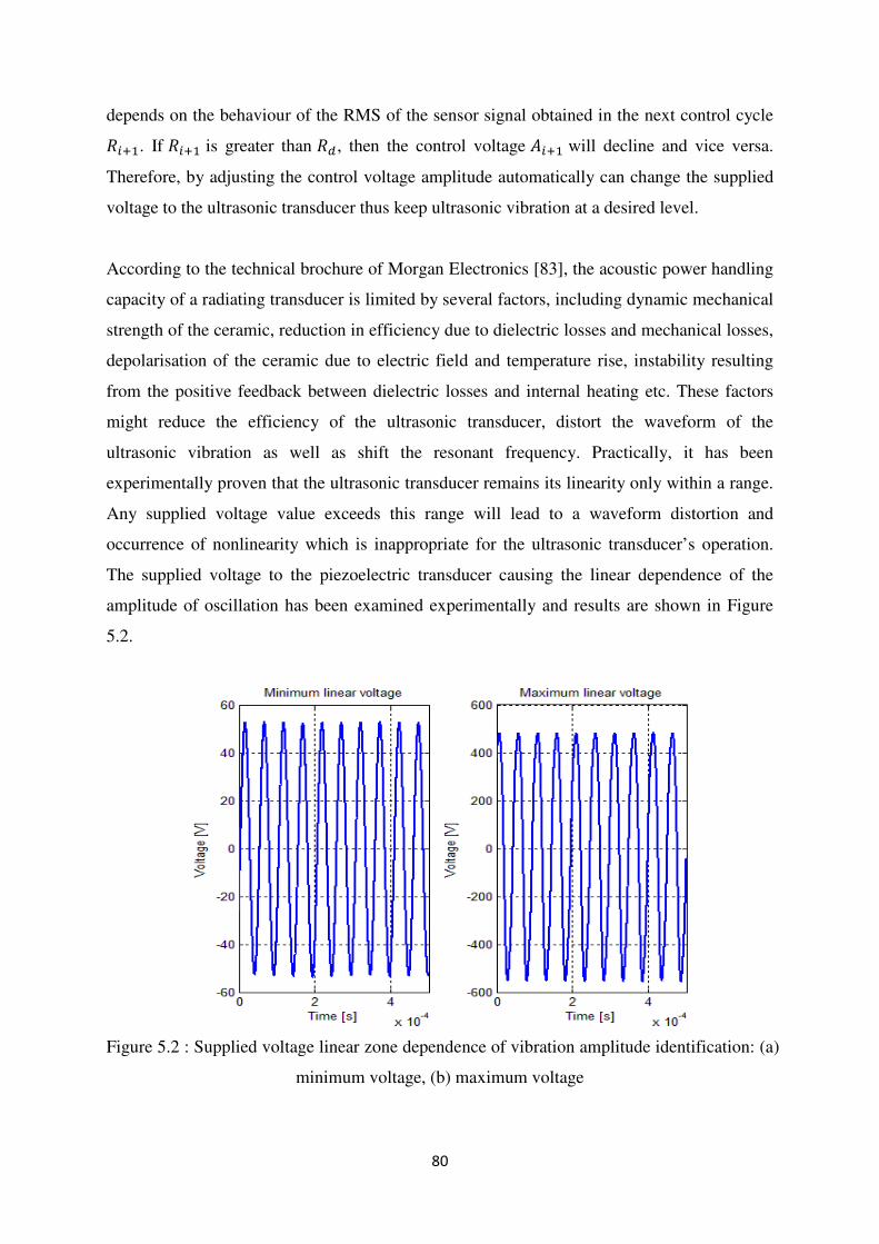
80
depends on the behaviour of the RMS of the sensor signal obtained in the next control cycle ��+1. If ��+1 is greater than �� , then the control voltage ��+1 will decline and vice versa.
Therefore, by adjusting the control voltage amplitude automatically can change the supplied
voltage to the ultrasonic transducer thus keep ultrasonic vibration at a desired level.
According to the technical brochure of Morgan Electronics [83], the acoustic power handling
capacity of a radiating transducer is limited by several factors, including dynamic mechanical
strength of the ceramic, reduction in efficiency due to dielectric losses and mechanical losses,
depolarisation of the ceramic due to electric field and temperature rise, instability resulting
from the positive feedback between dielectric losses and internal heating etc. These factors
might reduce the efficiency of the ultrasonic transducer, distort the waveform of the
ultrasonic vibration as well as shift the resonant frequency. Practically, it has been
experimentally proven that the ultrasonic transducer remains its linearity only within a range.
Any supplied voltage value exceeds this range will lead to a waveform distortion and
occurrence of nonlinearity which is inappropriate for the ultrasonic transducer’s operation.
The supplied voltage to the piezoelectric transducer causing the linear dependence of the
amplitude of oscillation has been examined experimentally and results are shown in Figure
5.2.
Figure 5.2 : Supplied voltage linear zone dependence of vibration amplitude identification: (a)
minimum voltage, (b) maximum voltage

81
It can be observed that the minimum voltage is 50� zero-to-peak in (a) and the maximum
voltage is around 500� zero-to-peak in (b). During experiments, the resonant regime has
been manually achieved by tuning the excitation frequency from a SFG-2110 Synthesized
Function Generator. After this, the amplification knob is adjusted accordingly to explore the
linear response of the ultrasonic vibration. Meanwhile, an electronic differential probe
GE8115 is used to measure the supplied voltage. The linear interval of the supplied voltage
which generates the linear ultrasonic vibrations is 50�~500� zero-to-peak. Therefore, each
set of the calculated control voltage amplitude in the autoresonant control system will be
checked to see whether it lies within the linear interval. For those exceed the upper limit,
500� will be used. Likewise, for those are less than the minimum, 50� will be used.
5.1.3 Amplitude-Phase Combined Control Algorithm
The combined amplitude-phase control algorithm enables the possibility of simultaneous
control of the phase shift and the control voltage amplitude. As introduced in section 5.1.1,
phase control is to maintain the resonant regime against the change in the feedback sensor’s
level during machining. Due to the fact that the amplitude-phase characteristic of an
ultrasonic transducer is flat near the resonant peak during machining, a slight change in phase
shift will not significantly affect the level of the ultrasonic vibration. Once there is a
significant drop in the level of oscillation because of essential applied load, amplitude control
needs to take part in to compensate the changes in the level of vibration and stabilise it.
In order to execute the switch between phase control and amplitude control, a new term �� is
introduced which represents the critical RMS of a feedback sensor signal. If the difference
between �� and the RMS in the ‘current’ control cycle �� is less than ��, then the sequence
flows through phase control algorithm and a new phase shift will be calculated and used for
next control cycle, in the meanwhile, control voltage amplitude remains as the previous cycle.
On the other hand, when �� exceeds �� by more than �� then the amplitude control algorithm
will be executed, i.e. a new control voltage amplitude is established according to equation
(5.1). However, phase shift remains unchanged. The combined amplitude-phase control
algorithm is illustrated in Figure 5.3.
The amplitude-phase combined control algorithm is a comprehensive control which aims at
keeping the ultrasonic vibration at a desired level during machining. Its basic principle has

82
been described, regarding the details of how phase shift is executed and control voltage is
changed, these will be introduced later. In the next section, a created Matlab-Simulink model
is introduced which consists of all elements and functions in the autoresonant control loop.
Figure 5.3 : Schematic diagram of amplitude-phase combined control algorithm
Reproduced and Revised From [68]
5.2 Autoresonant Control Model in Matlab-Simulink
Figure 5.4 : Autoresonant control system structure in Matlab-Simulink
Reproduced and Revised from [68]
The autoresonant control algorithm including phase control, amplitude control and combined
amplitude-phase control is illustrated in Figure 5.4. There are 8 function blocks in this
autoresonant control diagram and each of them will be introduced in details.

83
• Root-Mean-Square
Root-Mean-Square block is designed to collect the sensor samples and calculate the RMS for
each control cycle (will be defined by the author in the computer simulation). Input to the
block is the sensor signals and output from the block is the RMS and counter values (integer
number of oscillation periods which constitutes one control cycle). Depending on the
feedback type, a sensor signal could be the ultrasonic vibration at the end of the 2nd
step of an
ultrasonic transducer, a current or a power of a piezoelectric transducer. In order to compute
the RMS, following equation has been established:
��� = �1� ∫ �(�)2���0 (5.2)
In equation (5.2), RMS is the calculated Root-Mean-Square value of the ‘current’ control
cycle, � is the period of a control cycle which normally equals several hundreds of oscillation
periods. Selection of � will be introduced later. �(�) represents a sensor signal. Design of this
block can be found in Appendix III. Another notable point is that the RMS remains constant
within one control cycle and will not change until the beginning of next one.
• Phase Control
Phase control block is designed to adjust the phase shift according to the change in the RMS
of a sensor signal. As described in section 5.1.1 that phase control aims at keeping the
ultrasonic vibrations at theresonant state during Ultrasonic Machining (USM) process. In this
block, RMS of each control cycle is calculated based on the collected sensor samples. The
calculated RMS is compared with the RMS in previous cycle. If the RMS in the ‘current’
control cycle has increased from the previous one, then the phase shift will be added by 0.01
phase control unit. Otherwise a 0.01 phase control unit will be subtracted.
Inputs to the phase control block are the RMS values and counter values calculated by the
Root-Mean-Square block. Counter values are recorded as a number of oscillation periods
used to form one control cycle. Output from this block is the actual phase shift value
determined by the phase control algorithm which will be further processed by the phase
shifter block. The detailed structure of this block is shown in Appendix III.

84
• Amplitude Control
Amplitude control block is designed to control the autoresonant loop automatically with the
help of adjustment of an amplification gain in order to provide extra power to the ultrasonic
transducer to maintain the ultrasonic vibration at a desired level during an applied load. The
amplitude control block is designed to ensure the stability caused by the positive feedback.
The elaborated amplitude control value is calculated in equation (5.1). There are two inputs to
this block which are identical to those to the phase control block. Output from this block is
the calculated amplitude values which will be supplied into the amplifier block.
Consequently, function of the combined amplitude-phase control algorithm can be easily
implemented in association with phase control and amplitude control. The structure of the
amplitude control block is demonstrated in Appendix III.
• Mean Value
Mean value block is designed to calculate the mean values of a sensor signal which is well-
known as bias and then subtract it from the original sensor signals. For instance, the
ultrasonic vibration at the end of the 2nd
step of an ultrasonic transducer is asymmetric around
zero with an applied load which has been proven numerically and experimentally. However,
this procedure is negligible for current feedback and power feedback because electric signals
are symmetric. Input to this block is a sensor signal and output from this block is a symmetric
signal. An equation used to calculate the mean value of a sensor signal is shown below:
�(�)����� =1� ∫ �(�)���0 (5.3)
Where �(�) represents a sensor signal, � is one oscillation period and �(�)����� are the mean
values of the sensor signals. Technically, the mean values remain constant within one
oscillation period. The structure of the mean value block can be found in Appendix III.
• Sign
This block is designed to transform a sinusoidal wave into a square wave with a unity gain.
Basically, for a symmetric sinusoidal signal centred around zero, this block convers its half

85
positive wave into a positive straight unity line and transforms its half negative wave into a
negative straight unity line. Therefore, a set of square wave is generated with an exactly same
frequency as the original sensor signal. The converted square wave is prepared for the phase
shifter.
• Phase Shifter
Figure 5.5 : Principle of a phase shifter: (a) original square wave, (b) phase shift, (c) shifted
square wave
Reproduced and Revised from [68]

86
The phase shifter block is designed to shift the phase of the square wave signal according to
the phase shift value calculated from phase control block. It should be noted that this block is
only applicable to a square wave signal. The underlying principle of the phase shifter block is
shown in Figure 5.5.
The square wave signal with unity gains is the source of the phase shifter block which is
shown in (a) in Figure 5.5. Clearly, the original square wave signal consists of one rising
edge and one falling edge within one oscillation period. In order to shift the square wave and
generate a new one, the phase shift value calculated from the phase control block has been
used. In (b), the phase shift value has been multiplied by one oscillation period which is
expressed as a part of one oscillation period. Red dashed line represents one oscillation
period and dark blue dash dot line stands for the phase shift as a part of one oscillation
period. Once a rising edge is detected, the phase shifter performs an integration of a unity
constant and produces an inclined green solid line. The same procedure has been applied to a
falling edge which generates an inclined pink solid line. After each rising edge and falling
edge has been integrated, the phase shift is subtracted from the integration respectively.
Resultant inclined lines are shown in dash lines in green for rising edge and pink for falling
edge. These newly produced inclined lines meet zero at shifted points which establish a new
square wave with corresponding rising edges and falling edges shown (c). In this way, phase
shifting process is executed. The newly generated square wave can be further processed by an
amplifier. Theoretically, the phase shifter is able to handle a phase shift in an interval [0,2�].
Design of the phase shifter block in Matlab-Simulink can be referred to Appendix III.
• Amplifier
This block is designed to amplify the shifted square wave by multiplying a control voltage
calculated from the amplitude control block.
• Filtering
This block is designed to smooth the amplified square wave signal. Basically, this is done to
get rid of the high frequency components (noises) which might damage the piezoelectric
transducer. Practically, depending on the type of the control feedback, different filters should

87
be used. For instance, a low-pass filter is suitable for mechanical feedback. In contrast,
current feedback employs a band-pass Butterworth filter.
5.3 Control Strategies of Mechanical Feedback and Electrical
Feedback
As introduced in section 1.1 that there are mainly two types of control strategies depending
on sensor selections, which are either mechanical feedback with mechanical sensors or
electrical feedback with electrical sensors.
• Mechanical Feedback
Mechanical feedback employs a mechanical sensor to measure the
displacement/velocity/acceleration of an ultrasonic transducer during vibro-impact
• Electrical Feedback Sensor
Electrical feedback uses an electrical sensor to consider the electrical parameters as
feedback signals, which are either a current or a power of a piezoelectric transducer
In the case of mechanical feedback control, a mechanical sensor is chosen to measure the
mechanical vibration. The vibration signals could be displacement, velocity or acceleration.
Generally, mechanical sensors include a laser vibrometer, an accelerometer, an ultrasonic
microphone and an inductive (magnetic) sensor. A laser vibrometer and an inductive sensor
will be used in the autoresonant control in Ultrasonically Assisted Drilling (UAD). The
advantages of a mechanical sensor are it detects the ultrasonic vibration directly from the
cutting zone which guarantees the accuracy and reliability for autoresonant control design.
Despite such advantages, however, mechanical feedback sensors are difficult to be
appropriately mounted under ultrasonic machining conditions. Moreover, cost of mechanical
feedback sensors is relatively high.
For electrical feedback control aspect of view, an electrical sensor is selected to record the
electrical characteristics of an ultrasonic transducer during operation. Briefly, a current sensor
and a power sensor are available in experiments. Being different from mechanical feedback
sensors, electrical feedback sensors are cheaper and their possibility of remote operation is
preferable and suitable for industrial applications. Nevertheless, such sensors can only reflect
the ultrasonic vibration in an indirect way. In spite of this, electrical feedback sensors are

88
easier to be fixed on an ultrasonic transducer compared with mechanical feedback sensors.
Therefore, electrical sensors will also be employed in experiments.
As introduced before, an autoresonant control design relies on the amplitude-phase
characteristics of an ultrasonic transducer with an applied load, even though such
characteristics are time varying under machining conditions. The excitation force of an
ultrasonic transducer is produced through piezoelectric effect. However, for mechanical
feedback and electrical feedback, observation variables are different depending on the
locations on an ultrasonic transducer. Consequently, amplitude-frequency-phase
characteristics of these two types of control strategies are expected to show differently. For
the ultrasonic transducer model displayed in Figure 4.9, the excitation force produced by the
piezoelectric transducer is directly applied to the 1st step concentrator, whereas, depending on
the type of feedback control strategies, observation points for optimal phase shift are:
• For mechanical feedback, an inductive sensor or a laser vibrometer measures the
ultrasonic vibration signal at the end of the 2nd
step of an ultrasonic transducer which
indicates the observation variable is the absolute displacement of the 2nd
step �2.
• For electrical feedback, a current sensor measures the current of an piezoelectric
transducer. According to equation (4.63) and equation (4.73), current is computed as
the derivative of the electrical charge, which is related to both the excitation force �0
and the input voltage �. The excitation force �0 can be expressed as a function of the
displacement of the piezoring �0 and the displacement of the 1st step concentrator �1.
In addition, the input voltage � can be transformed as a function of the excitation
force �0 and the piezoring displacement �0 . Therefore, the observation point for
electrical feedback is the absolute displacement of the 1st
step �1.
In order to obtain the amplitude-phase-frequency characteristics for both observation
variables �1 and �2 , two methods can be used. The 1st
method relies on the frequency
response of the linearization of the ultrasonic transducer model shown in Figure 4.9. The
linear relationship between the input and output of the ultrasonic transducer can be expressed
as a transfer function. In comparison, the 2nd
method is to employ the ultrasonic transducer
differential equations shown from (4.71) to (4.73). A further transformation of these
differential equations will be executed to acquire the amplitude-phase-frequency

89
characteristics for both observation points. Features of the amplitude-phase characteristics for
both observations points and their implications will be analysed. In addition, comparisons and
discussions of the results for these two methods will also be involved. After the analysis of
the amplitude-phase-frequency characteristics for both feedback types, amplitude-frequency
characteristics of mechanical feedback signal, i.e. the displacement of 2nd
step �2 and
electrical feedback signal i.e. the current and power of the piezoelectric transducer will be
calculated respectively. Similarly, there are 2 methods to perform the calculations. One of
them is to numerically analyse and utilize the dynamic different equations of the ultrasonic
transducer from (4.71) to (4.73). Another approach is to simulate the ultrasonic transducer
Matlab-Simulink model shown in Figure 4.10 within an interested frequency range. Results
of these 2 methods will be compared and further analysed. In the end, the experimental
measurements will be brought in to compare with the simulation results.
5.3.1 Amplitude-Phase-Frequency Characteristics Calculation
Using Linearization of Ultrasonic Transducer Model
Theoretically, for a Linear-Time-Invariant (LTI) system with a transfer function �(�), its
output with a sine wave indicates the input is also a sine wave, but with a different amplitude
and phase. Assuming that the input to the system is �(�) and the output is �(�), then the
output response at a particular frequency � = 2�� is given by the gain and the phase of the
frequency response �(��) at that frequency �. For a system shown in Figure 5.6, assuming
the input and output after the initial transients are:
�(�) = ����(��)�(�) = ����(�� + �) (5.4)
Figure 5.6 : A Linear-Time-Invariant (LTI) system
The gain and the phase at a particular frequency � are then given by:
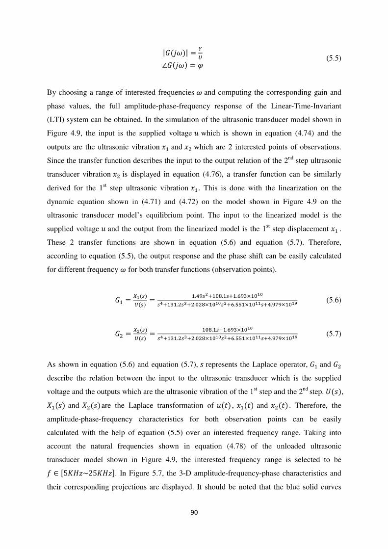
90
|�(��)| =��∠�(��) = � (5.5)
By choosing a range of interested frequencies � and computing the corresponding gain and
phase values, the full amplitude-phase-frequency response of the Linear-Time-Invariant
(LTI) system can be obtained. In the simulation of the ultrasonic transducer model shown in
Figure 4.9, the input is the supplied voltage � which is shown in equation (4.74) and the
outputs are the ultrasonic vibration �1 and �2 which are 2 interested points of observations.
Since the transfer function describes the input to the output relation of the 2nd
step ultrasonic
transducer vibration �2 is displayed in equation (4.76), a transfer function can be similarly
derived for the 1st step ultrasonic vibration �1. This is done with the linearization on the
dynamic equation shown in (4.71) and (4.72) on the model shown in Figure 4.9 on the
ultrasonic transducer model’s equilibrium point. The input to the linearized model is the
supplied voltage � and the output from the linearized model is the 1st step displacement �1 .
These 2 transfer functions are shown in equation (5.6) and equation (5.7). Therefore,
according to equation (5.5), the output response and the phase shift can be easily calculated
for different frequency � for both transfer functions (observation points).
�1 =�1(�)�(�)
=1.49�2+108.1�+1.693×10¹⁰�4+131.2�3+2.028×10¹⁰�2+6.551×10¹¹�+4.979×10¹⁹ (5.6)
�2 =�2(�)�(�)
=108.1�+1.693×10¹⁰�4+131.2�3+2.028×10¹⁰�2+6.551×10¹¹�+4.979×10¹⁹ (5.7)
As shown in equation (5.6) and equation (5.7), � represents the Laplace operator, �1 and �2
describe the relation between the input to the ultrasonic transducer which is the supplied
voltage and the outputs which are the ultrasonic vibration of the 1st step and the 2
nd step. �(�), �1(�) and �2(�)are the Laplace transformation of �(�) , �1(�) and �2(�) . Therefore, the
amplitude-phase-frequency characteristics for both observation points can be easily
calculated with the help of equation (5.5) over an interested frequency range. Taking into
account the natural frequencies shown in equation (4.78) of the unloaded ultrasonic
transducer model shown in Figure 4.9, the interested frequency range is selected to be � ∈ [5���~25���]. In Figure 5.7, the 3-D amplitude-frequency-phase characteristics and
their corresponding projections are displayed. It should be noted that the blue solid curves

91
represent the characteristics when the ultrasonic vibration of the 2nd
step �2 is the observation
point; the red dashed curve lines show the characteristic when the ultrasonic vibration of the
1st step �1 is the observation point. It should be noted that, the phase values for both curves
are all positive. Practically it means the output (the ultrasonic vibration of the 1st step �1 and
the 2nd
step �2) of the ultrasonic transducer lags the input supplied voltage �.
Figure 5.7 : Amplitude-Phase-Frequency characteristics for two observation points �1 and �2
of the linearization method: (a) 3-D amplitude-phase-frequency, (b) amplitude-frequency, (c)
phase-frequency, (d) amplitude-phase
In order to verify the accuracy of the calculated amplitude-phase-frequency characteristics for
both observation points, another method can be adopted in the next section which is based on
the transformation of the dynamic differential equations of the ultrasonic transducer.
5.3.2 Amplitude-Phase-Frequency Characteristics Calculation
Using Dynamic Differential Equations of Ultrasonic
Transducer Model

92
Since the input to the ultrasonic transducer model is the supplied voltage �, it is sensible to
combine the piezoelectric transducer model described in section 4.2 with the 2-DOF
concentrator model shown in Figure 4.7. Recalling the piezoelectric transducer equations:
�0 =1�01 �0 + �02��0 = �1(�̇1 − �̇0) + �1(�1 − �0)
(5.8)
Where � is supplied voltage, �0 is the small displacement of a piezoring, � is the electrical
charge stored in a piezoring and �0 is the interaction force (actuation force) between a
piezoring and the 1st step concentrator. �01,�02 are the known parameters which are �01 =13.84×10⁻¹¹ and �02 = 3.4 × 10⁻¹⁰ . �1 is the displacement in the middle of the 1
st step
concentrator, �1 and �1 are concentrator stiffness and damping coefficient of the 1st step.
Observing the expression of �0 in equation (5.8), it implies that the piezoelectric transducer
(piezoring) has two components. One of them is the scaled supplied voltage �02�, another
component is 1�01 �0. It can be considered that �01 is the contact stiffness of one piezoelectric
ring which interacts with the 1st step concentrator at force �0. However, the interaction force �0 is related to both stiffness and damping coefficient of the 1
st step concentrator, which
means theoretically the stiffness �01 and �1 are not connected simply in series. As a result, �01 is connected to the 1st spring-damper set directly without any mass in the middle which is
shown in (b) in Figure 5.9. However, this is not a reasonable linkage between dynamic
components because a mass is indispensable in a dynamic system.
As known to all, a dynamic system without a mass attached is not a purely mechanical
system. On the other hand, however, as can be seen in Figure 5.8 that the contributions to
interaction force �0 from damper �1 and spring �1 are significantly different. Contribution
from damper �1 (red curve) can be neglected compared to contribution from �1 (blue curve).
Therefore, the approximation can be made that the interaction force �0 is only generated by
the spring �1. Consequently, the stiffness �01 can be considered to connect in series with the
stiffness �1 and these two springs are arranged in parallel with the damper �1 which is
demonstrated in (c) in Figure 5.9 with the supplied voltage � acting as the input signal.

93
The dynamic partial differential equations (4.71) and (4.72) of the ultrasonic transducer hence
can be further modified into:
�1�̈1+�1(�̇1 − �02�̇)+��(�1 − �02�) + �2(�̇1 − �̇2) + �2(�1 − �2) = 0�2�̈2 − �2(�̇1 − �̇2) − �2(�1 − �2) = 0 (5.9)
Where in equation (5.9), �� is the effective contact stiffness of 2 springs connected in series.
Supplied voltage � acts as the input to the ultrasonic transducer which can be assumed as the
following form:
�� =�01�1�01+�1 (5.10) � = ����� (5.11)
Figure 5.8 : Actuation force contribution from the stiffness and damping coefficient
Substitute equation (5.11) into equation (5.9) produces:
�1�̈1+(�1 + �2)�̇1+(�� + �2)�1 − �2�̇2 − �2�2 = ���02����� + �1�02��������2�̈2 − �2�̇1 + �2�̇2 − �2�1 + �2�2 = 0 (5.12)
Rearranging the above equations into matrix form gives:
��̈ + ��̇ + �� = ����� (5.13)

94
Where � = ��1�2� is the displacement vector of the ultrasonic transducer, � = ��1 0
0 �2� is
the mass matrix,� = ��1 + �2 −�2−�2 �2 � is the damping matrix, � = ��� + �2 −�2−�2 �2 � is the
stiffness matrix and � = ����02� + �1�02���0
� is the actuation force vector. After the
transient response, the ultrasonic vibrations will gradually arrive at the steady states with the
following forms:
�1 = �1����−�1 = �1�����2 = �2����−�2 = �2���� (5.14)
Figure 5.9 : Ultrasonic transducer model transformation: (a) original ultrasonic transducer, (b)
ultrasonic transducer with input supplied voltage (non-mechanical), (c) ultrasonic transducer
with input supplied voltage (mechanical)
Where �1 and �2 are the ultrasonic vibration amplitudes of the 1st step and 2
nd step
concentrator, �1 and �2 are the phase shifts with respect to the actuation force (supplied

95
voltage), �1 and �2 are the complex vibration amplitudes of the 1st step and 2
nd step
concentrator which take into account phase shifts. By replacing the expressions of �1 and �2
into equation (5.13), the relation between the system vibrations � and the actuation force
(supplied voltage) � can be obtained:
(−�2� + ��� + �)�� = � (5.15)
�� = ��1�2� is the complex vibration amplitude vector. Dynamic stiffness is equal to the ratio
between a force which acts on the measurement point and the complex displacement
amplitude [8]. Therefore, the dynamic stiffness matrix of the ultrasonic transducer becomes:
�(��) = [−�2� + ��� + �] (5.16)
Figure 5.10 : Amplitude-Phase-Frequency characteristics for two observation points �1 and �2 of dynamic differential method: (a) 3-D amplitude-phase-frequency, (b) amplitude-
frequency, (c) phase-frequency, (d) amplitude-phase

96
Therefore, the complex vibration amplitude �1, �2 and the corresponding phase shift �1, �2
can be calculated with the same interested frequency range � ∈ [5���~25���] . The
amplitude-phase-frequency characteristics of the ultrasonic transducer for both observation
variables are shown in Figure 5.10. Similarly, the blue solid curves show the observation
point of the ultrasonic vibration of the 2nd
step concentrator �2 and red dashed curves
illustrate the observation point of the ultrasonic vibration of the 1st
step concentrator �1. In
addition, it can be observed clearly that Figure 5.7 and Figure 5.10 have a close agreement in
shape, resonant frequency and magnitude. Therefore, both methods are applicable and
feasible for amplitude-phase-frequency characteristics calculation of the ultrasonic transducer.
5.3.3 Amplitude-Phase Characteristic Analysis for both
Observation Points
Since the autoresonant control strategy relies on the amplitude-phase characteristic,
amplitude-phase characteristics for both feedback types (observation points) are enlarged for
successive analysis which is shown in Figure 5.11. Blue curve represents the characteristic
when the 2nd
step ultrasonic vibration �2 is selected to be observed and red dashed curve
stands for the observation point of the 1st step ultrasonic vibration �1. Several features can be
concluded from this picture.
Figure 5.11 : Amplitude-phase characteristic for both observation points �1 and �2

97
• Both curves present a gently sloping bell shape near the resonant peak. In comparison,
the amplitude-frequency characteristic shown in (b) in either Figure 5.7 or Figure 5.10
exhibits an extremely sharp peak near the resonant frequencies which strongly
suggests the possibility and feasibility of the employment of phase control.
• At phase shift �2, one of the vibration magnitudes of the 1
st step concentrator and the
vibration amplitude of the 2nd
step concentrator demonstrates a several hundred
micrometres value which seems unreasonably large. This was not observed during
experiments with resonant frequency around 8.5���. This is due to the limitation of
simplification of the ultrasonic transducer into a 2-DOF model. In other words, a
simplified 2-DOF model is only valid within a certain range in terms of resonant
frequency and vibration amplitude. The performance of a 2-DOF model is not
guaranteed for those frequencies out of the range.
• The blue curve which represents the characteristic of the ultrasonic vibration �2 at the
end of the 2nd
step concentrator displays a single-valued property. In other words, one
phase shift corresponds to fixed amplitude. In contrast, the red-dashed curve that
stands for the characteristic of the ultrasonic vibration in the middle of the 1st step
concentrator �1 exhibits certain ambiguity which indicates one phase shift reflects
three different vibration amplitudes.
In Figure 5.11, it is clear that one phase shift generates 3 oscillation regimes with different
vibration amplitudes when the 1st step concentrator’s ultrasonic vibration �1 is selected to be
the observation point. These 3 oscillation regimes are excited respectively with 3 different
frequencies shown in (b) in Figure 5.7 and Figure 5.10. The first 2 regimes are the products
of the 1st and 2
nd oscillation modes and the 3
rd regime with the lowest amplitude is known as
an ‘anti-resonant’ regime. Nonetheless, despite the first 2 resonant regimes can be seen
clearly, the ‘anti-resonant’ regime seems less obvious. Therefore, the display of amplitude of
(b) in Figure 5.7 and Figure 5.10 has been further revised into logarithm when the 1st step
concentrator’s ultrasonic vibration �1 is involved both in excitation and observation.
Figure 5.12 shows the amplitude-frequency characteristic when the 1st step concentrator’s
ultrasonic vibration �1 is selected to be the excitation signal and the observation point.
Clearly, 2 resonant regimes with resonant frequencies 8.5��� and 21.0��� corresponds to

98
the first 2 vibration regimes shown in Figure 5.11. The 3rd
vibration regime displays a distinct
property of an ‘anti-resonant’ regime which arrives at the valley peak and this ‘anti-resonant
regime’ is the one shown in Figure 5.11 with the lowest magnitude. According to numerical
calculation, the ‘anti-resonant’ vibration regime has a anti-resonant frequency 17.0���.
Figure 5.12 : Amplitude-frequency characteristic of 1st step as excitation and observation
In the following sections, stability analysis for these 3 vibration regimes will be executed in
computer simulation. Generally speaking, the procedure for the stability investigation is that
the ultrasonic transducer is initially excited with 3 vibration regimes’ resonant frequencies.
After the ultrasonic vibration arrives at a steady state level, the loop is closed and the
ultrasonic vibration of the 1st step concentrator �1 is employed as the feedback signal.
Meanwhile, changes in the ultrasonic vibration for both the 1st step �1 and the 2
nd step �2 are
monitored. Theoretically, a continuation of the ultrasonic vibration is expected after the loop
is closed which confirms a stability of the corresponding vibration regime. In comparison, a
sudden change (disappearance or essential increase) in the ultrasonic vibration signal
concludes instability.
5.3.3.1 Stability Analysis of 1st
Resonant Regime
As calculated before, the 1st resonant regime has a resonant frequency 8.5���. Therefore,
the ultrasonic transducer model is initially excited with this frequency. When the ultrasonic
vibration arrives at its steady-state, the loop is closed with the ultrasonic vibration of 1st step

99
�1 acting as the feedback signal and the phase shift is tuned to be near �2 as indicated in
Figure 5.11. Simultaneously, the ultrasonic vibrations of both steps of the ultrasonic
transducer are recorded accordingly.
Figure 5.13 : Stability analysis of 1st resonant regime with observation point �1 : (a)
amplitude response of 1st step, (b) amplitude response of 2
nd step
In Figure 5.13, ultrasonic vibrations of the 1st step and 2
nd step ultrasonic transducer are
displayed. As can be seen, the ultrasonic vibrations for both steps are gradually boosted up
and reach their steady states at 0.4sec. The steady state vibration amplitudes for both steps are
equivalent to the 1st peak values shown in Figure 5.11 (blue solid curve and red dashed
curve). After the ultrasonic transducer oscillates for a reasonably long time, the loop is closed
at 1.0sec. Clearly, both steps continue to oscillate as before even though the level of
oscillations is increased by certain amount which is likely caused by the filter within the loop.
The filter is used to rectify an amplified and phase-shifted square wave to create a quasi-
sinusoidal signal with reasonable magnitude which is then supplied into the ultrasonic
transducer. Filter design will be described elaborately in Chapter Six. Consequently, since the
self-sustaining process has not lead to a sudden change to the ultrasonic vibration for both
steps, it can be concluded that the 1st resonant regime is stable.

100
5.3.3.2 Stability Analysis of 2nd
Resonant Regime
Figure 5.14 : Stability analysis of 2nd
resonant regime with observation point �1: (a)
amplitude response of 1st step, (b) amplitude response of 2
nd step
The 2nd
regime oscillates at a resonant frequency 21.0��� which is shown in Figure 5.12.
Consequently, the supplied voltage � uses this frequency to initially boost up the ultrasonic
transducer. The operation procedure is exactly the same as the description in section 5.3.3.1.
In Figure 5.14, the 1st step and 2
nd step ultrasonic vibrations are illustrated. Clearly, both steps
ultrasonic vibrations quickly climb to their corresponding steady states which take less than
0.1secs. The steady state oscillation amplitudes have equal values as the amplitudes shown in
Figure 5.11. After this, the ultrasonic transducer keeps vibrating before the loop is closed
which takes place at 1.0sec. Both steps continue to vibrate as usual in spite of a slight
increase in the amplitude, which again, is caused by the filtering process. As a result, the 2nd
resonant regime is also a stable vibration regime because the closed loop system produces no
essential change to the ultrasonic vibration amplitudes for both steps.
5.3.3.3 Stability Analysis of Anti-Resonant Regime
The ‘anti-resonant’ frequency shown in Figure 5.12 is approximately 17.0���. Hence, the
ultrasonic transducer is activated with this frequency initially. Procedure remains same. In

101
Figure 5.15, results are shown. In the beginning, the ultrasonic transducer is actuated and the
ultrasonic vibrations seem small which corresponds to the ‘anti-resonance’ values for both
steps. At 1.0sec, the loop is closed and the 1st step ultrasonic vibration acts as the feedback
signal. It can be observed that the ultrasonic vibrations suddenly soar into huge values for
both steps. The closed loop ultrasonic vibration steady state values equal the steady state
values of the 1st resonant regime. In other words, the feedback system ‘jumps’ from the ‘anti-
resonant’ regime to the 1st resonant regime. Therefore, as a ‘jump’ phenomenon takes place
in the closed loop system, the ‘anti-resonant’ regime is instable.
Figure 5.15 : Stability analysis of ‘anti-resonant’ regime with observation point �1: (a)
amplitude response of 1st step, (b) amplitude response of 2
nd step
5.3.3.4 Conclusion of Stability Analysis
According to stability analysis of the 1st resonant regime, 2
nd resonant regime and the ‘anti-
resonant’ regime, it can be concluded that both resonant regimes can be maintained under
phase control. In contrast, the ‘anti-resonant’ regime exhibits a ‘jump’ to the 1st
resonant
regime in the closed loop which indicates the ‘anti-resonant’ regime is unstable and
physically cannot be attained under phase control.

102
Even though both resonant regimes are stable and can be controlled under phase control, one
phase shift corresponds to 2 different vibration amplitudes when the 1st step ultrasonic
vibration �1 participates in both excitation and observation. This non-single valued property
will cause ‘confusion’ to the closed loop system under phase control when the current is
selected as the feedback signal. Therefore, a filtration process is strongly recommended for
the electrical feedback in order to pick up the desired vibration regime whilst filter out the
others. According to the computer simulation, this filtration process brings tremendous
problems to the control design as a filter can shift the phase of the amplified square wave.
This additional phase shift introduced by a filter is uncontrollable and unchangeable with
autoresonant control. Filter selection and electrical feedback will be investigated and
examined closely with mechanical feedback later.
5.3.4 Amplitude-Frequency Characteristics Investigation for
Ultrasonic Vibration, Current and Power
It has been introduced in section 5.3 that mechanical feedback and electrical feedback employ
different sensor signals. Mechanical feedback uses a mechanical sensor to measure the
ultrasonic vibration. In contrast, electrical feedback employs electrical signals to form the
feedback loop which can be either a current or a power of a piezoelectric transducer. In order
to examine the effect on the control system design for these 2 feedback types, amplitude-
frequency characteristics of the ultrasonic vibration, current and power have been
numerically and experimentally obtained. Basically, there are 2 methods to calculate the
amplitude-frequency characteristics numerically. One method relies on the dynamic
differential equations described in section 5.3.2. Dynamic equations for current and power
can be subsequently deducted according to the current expression in equation (4.63). Another
way is to simulate the ultrasonic transducer model in Matlab-Simulink within an interested
frequency range then record the ultrasonic vibration, current and power respectively. Apart
from the numerical computation, an experiment has been performed to record 3 signals. In
the end, comparison and analysis of the amplitude-frequency characteristics for mechanical
feedback and electrical feedback will be involved.
5.3.4.1 Amplitude-Frequency Characteristics Calculation Using
Dynamic Differential Equations of Ultrasonic Transducer

103
As shown in Figure 5.8 that the interaction force �0 contribution from the elastic spring �1 is
essential compared to the contribution from the viscous damper �1. Therefore, the interaction
force �0 displayed in equation (5.8) can be modified:
�0 =1�01 �0 + �02��0 ≈ �1(�1 − �0)
(5.17)
Recalling the electrical charge � in equation (4.63) of the piezoelectric transducer, by taking
the derivative to the charge with respect to time obtains the current which has the following
form:
� = �03�0 + �04�� = �̇ = �03�̇0 + �04�̇ (5.18)
Where �03 = 3.4 × 10⁻¹⁰ and �04 = 2.1 × 10⁻⁹ are the coefficients shown in equation
(4.63), � is the electrical charge, � is the supplied voltage and � is the current flows through
the piezoelectric transducer. After rearrangement of equation (5.17), expression of the
interaction force �0 in terms of �1 and � can be obtained as:
�0 =�01�1�1−�01�02�1��01+�1 (5.19)
Substituting the expression of �0 shown in equation (5.19) into equation (5.18) produces the
current:
� =�01�03�1�̇1+(�01�04+�04�1−�01�02�03�1)�̇�01+�1 (5.20)
Thus, the current expression is derived. It is presumed that after the ultrasonic transducer
passes its transient response and reaches the steady state, the current also arrives at its steady
state which has following form:
� = �����−�� = ��̅��� (5.21)

104
� is the current amplitude and �� is the phase shift between the current � and the supplied
voltage �, � ̅is the complex amplitude of the current � which takes the phase shift �� into
account. Moreover, the steady state ultrasonic vibration of the 1st step concentrator and the
supplied voltage � has been assumed in section 5.3.2. Therefore after substitution of equation
(5.21) into equation (5.20) allows:
� ̅ = ���01+�1 [�01�03�1��1 + (�01�04 + �04�1 − �01�02�03�1)�] (5.22)
Hence, the amplitude-frequency characteristics for the current can be calculated within the
interested frequency range. In the case of power, it is assumed to be a sinusoidal signal at
steady state, and then it can be calculated in the following format:
� =1� ∫ �����0 (5.23)
� is the average power of the ultrasonic transducer, � is the supplied voltage and � is the
current, � is the calculated period of oscillations. Assume the supplied voltage � and the
current � with following form: � = ������ = �����−�� (5.24)
Substituting equation (5.24) into equation (5.23) gives the expression of the average power :
� =12�����(��) =
12��ℜℯ������ =12ℜℯ(��) (5.25)
Where ℜℯ represents the real part of a complex number. Since the expressions of the voltage � and current � have been introduced in equation (5.24), the average power can then be
calculated successively by taking the real part of the product of the supplied voltage � and the
current �.
In Figure 5.16, the amplitude-frequency characteristics of the ultrasonic vibration at the end
of the 2nd
step concentrator, current and average power are shown respectively. 3 curves are
obtained within an interested range of � ∈ [20.5���~21.5���] which centres around the
ultrasonic vibration resonant frequency 21.0���. It can be observed clearly that the resonant

105
peak of the ultrasonic vibration (a) has an accurate coincidence with the peak in average
power (b) as well as with current (c) even if the current seems to have a slight reflection after
the minimal value. As described before, an autoresonant control system always targets at the
resonant regime. Since three signals coincide at the same resonant frequency, the supplied
voltage � used to drive the ultrasonic transducer in the feedback loop in Matlab-Simulink
model for mechanical feedback, current feedback and power feedback is supposed to have a
similar value. This can be verified in Chapter Six. In next section, the characteristics results
acquired from computer simulation will be demonstrated.
Figure 5.16 : Amplitude-Frequency characteristics of three signals using dynamic equation
method: (a) ultrasonic vibration of 2nd
step concentrator, (b) power, (c) current
5.3.4.2 Amplitude-Frequency Characteristics Calculation Using
Computer Simulation of Ultrasonic Transducer
Another approach used to calculate the amplitude-frequency characteristics for the ultrasonic
vibration of the 2nd
step �2, current and power is to use computer simulation of an ultrasonic
transducer model. During simulation process, an interested frequency interval is � ∈[20.5���~21.5���] . The ultrasonic vibration at the end of the 2
nd step concentrator,
current and power of the piezoelectric transducer are recorded literally.

106
Figure 5.17 demonstrates the amplitude-frequency characteristics of the ultrasonic vibration
of the 2nd
step, average power and current of the piezoelectric transducer. As can be seen, the
ultrasonic vibration meets at a same resonant frequency with the current and the power which
indicates a similar supplied voltage � in feedback loop. In conclusion, both approaches used
to calculate amplitude-frequency characteristics of mechanical feedback signal and electrical
feedback signals are accurate and effective. In order to verify the preciseness of the
amplitude-frequency characteristics obtained for numerical model, an experiment on an
electromechanical ultrasonic transducer has been carried.
Figure 5.17 : Amplitude-Frequency characteristics of three signals using computer simulation
method: (a) ultrasonic vibration of 2nd
step concentrator, (b) power, (c) current
5.3.4.3 Amplitude-Frequency Characteristics of Experiment
In order to acquire the characteristics of an electromechanical ultrasonic transducer (without a
drill bit attached), an experiment has been performed and the schematic diagram of the
experimental setup is shown Figure 5.18. To start with the experiment, a swept sine wave is
generated from a SFG-2110 Synthesized Function Generator with reasonable amplitude.
Before the swept sine wave is supplied into a universal amplifier, the resonant frequency ��
of the ultrasonic vibration is manually explored by slowly changing the excitation frequency.
Therefore, an interested frequency range can be defined which centres around ��. The swept

107
sine wave is fed to a universal amplifier to amplify the driving signal at a primary stage. After
this, the amplified signal is supplied into a universal matchbox (transformer) to adjust the
high impedance of the universal amplifier to the low impedance of the ultrasonic transducer
(structure and explanation of the universal matchbox will be introduced in Appendix I). As a
result, a high voltage is generated by the universal matchbox (transformer) which is used to
drive the ultrasonic transducer. A GE8115 Differential Probe is employed to collect the
supplied voltage signals, the measurement range of the differential probe is −1500�~1500�. Furthermore, a LEM HEME Ltd PR 30 Current probe is connected in
order to acquire samples of the current flows through the piezorings. In addition, a power
sensor has been manufactured to calculate the product of the voltage � and the current � in
real time. After the instantaneous power has been collected, the average power of the
ultrasonic transducer can be computed using the following equation:
P =1T∫ uidt
To (5.30)
Figure 5.18 : Experimental schematic diagram to acquire amplitude-frequency characteristics
of ultrasonic vibration, current, power and voltage

108
� represents the average power, � is one oscillation period, � and � are the voltage and the
current. Apart from the electrical signals, the actual mechanical vibration at the end of the 2nd
step concentrator �2 is measured by a Polytec Vibrometer. This is realized by shining a laser
beam to the vertical surface of a flatly attached reflection film at the end of the 2nd
step
concentrator. Eventually, both mechanical signal and electrical signals are stored in a
PicoScope which is further connected to a computer for data processing. The increment of the
excitation frequency has been chosen as 0.01��� in order to allow sufficient frequency
points to be captured. This high resolution is important especially for those characteristics
near resonance.
Results obtained from experiment are showed in Figure 5.19. As can be seen, the ultrasonic
vibration’s resonance (a) coincides with the resonance of the average power (b) and the
current (c). Besides, the shape of 3 signals conforms to the numerical curves which enhance
the numerical results. The distinction between the numerical calculation and the experiment
is the shift in the resonant frequency. Nonetheless, a simple 2-DOF ultrasonic transducer
model exhibits a high validity and similarity to the electromechanical ultrasonic transducer in
spite of such resonant frequency shift.
Figure 5.19 : Amplitude-Frequency characteristics obtained experimentally: (a) ultrasonic
vibration of 2nd
step concentrator, (b) power, (c) current

109
The supplied voltage � is recorded simultaneously which is shown in Figure 5.20. Clearly,
the resonant frequency of the voltage signal also coincides with other 3 signals. However, the
shape of the voltage shows a more drastic change over the resonant frequency compared with
the current. The maximum voltage is nearly 300� where the minimum voltage is around 20�.
At the frequency range beyond resonance, voltage remains around 100�.
Figure 5.20 : Amplitude-Frequency characteristic of the supplied voltage
As a matter of fact, the supplied voltage � depends on several factors. One of them is the air
gap distance between two ferrite cores in the universal matchbox. It has been experimentally
found by adjusting the position of one ferrite is able to change the voltage level and signals
wave forms significantly. The ultrasonic vibration amplitude can be optimized (maximized)
by adjusting the position of the ferrite core. Investigation and optimization of the universal
matchbox can be found in Appendix I. The supplied voltage � has been selected as 200� in
the numerical simulation which is a normal working voltage of the ultrasonic transducer at
resonance.
5.4 Summary
In this chapter, the algorithms of phase control, amplitude control and phase-amplitude
combined control have been introduced. A Matlab-Simulink model describes these
algorithms is illustrated and each function block is explained and analysed in details.

110
In order to better understand the autoresonant control system, the characteristics for both
mechanical feedback and electrical feedback systems are obtained with a number of reliable
and feasible methods. Results of these methods show a high similarity with each other which
confirmed the validity and accuracy of the 2-DOF model. Due to the fact that the key
principle of the autoresonant control is to control the phase between the input and output of
the ultrasonic transducer, the amplitude-phase characteristics for mechanical feedback
observation point �2 and electrical observation point �1 are depicted. The conclusion implies
that the amplitude-phase characteristic of the mechanical feedback observation point �2
displays a bell-shape feature with a one-to-one mapping between the phase shift value and the
amplitude value. This suggests that a simple low pass filter is able to rectify the square wave
to act as the supplied voltage. In contrast, the amplitude-phase characteristic for the electrical
feedback observation point �1 exhibits an ambiguity property. In other words, the non-single
value feature indicates that one phase shift reflects 3 different oscillation regimes. These
regimes’ stabilities have been investigated numerically which recommends a proper filtration
process in order to pick up the desired oscillation regime.
In addition, the amplitude-frequency characteristics for mechanical feedback vibration �2 and
electrical feedback signals (current � and average power � ) are computed in numerical
simulation with several methodologies. These characteristics have been recorded in
experiment too in order to validate the numerical results. As mechanical feedback signal
reflects the ultrasonic vibration �2 in a direct way whilst electrical feedback only reflect it in
an indirect way, this theoretical investigation and experimental analysis comparison seems
necessary for the impact these two feedback types may impose on the autoresonant control
system design.

111
Chapter Six Control Evaluation in Numerical Simulation
This chapter is dedicated to the numerical simulation of the control evaluation for several
feedback control strategies. Before mechanical feedback and electrical feedback are tested,
frequency controlled ultrasonic vibration will be explored.
Mechanical feedback employs a mechanical sensor to measure the actual ultrasonic vibration
at the end of the 2nd
step concentrator �2 and apply it as a feedback signal. Since mechanical
feedback directly reflects the ultrasonic vibration, it is supposed to present a better control
than electrical feedback. In contrast, electrical feedback uses electrical characteristics of a
piezoelectric transducer which can be either a current or a power as a feedback signal. Due to
the fact that electrical signals reflect the ultrasonic vibration in an indirect way, this type of
feedback control is assumed to present a more inferior result than mechanical feedback.
Basically, the effectiveness of electrical feedback control relies on the dynamic coupling
(formula) between electrical parameters and mechanical vibration.
An autoresonant control system is designed to keep the ultrasonic vibration at the end of 2nd
step �2 at a desired level during vibro-impact process. In numerical simulation,the applied
load will be changed and the RMS of the sensor signals will be monitored for each control
cycle. Generally speaking, as can be seen in Figure 4.17, there are several parameters in
Kelvin-Voigt model affecting the applied load (feed force). One of them is the contact
stiffness � which is an essential contributor to the loading; the other one is the viscous
damper � which an insignificant contributor to the applied load. In addition, change in initial
interference ∆ is also a subject of interest for control evaluation. Therefore, two types of tests
are evaluated: change in contact stiffness � and change in initial interference ∆ between the
ultrasonic transducer and the applied load.
The range of the change for the increase in contact stiffness is � ∈ [1 × 10⁸�/�~7 ×
108�/�] with an increment 1 × 10⁸�/�. The interval of the change in initial interference
is ∆∈ [−2 × 10⁻⁷�~ − 1 × 10⁻⁵�] with an increment −2 × 10⁻⁶� . Changes for both
contact stiffness � and initial interference ∆ are applied to mechanical feedback, current
feedback and power feedback respectively. It should be noted that in numerical simulation,

112
the ultrasonic transducer is not attached with a drill bit. In other words, tool effect is not
explored and control evaluation is purely carried out on the ultrasonic transducer.
6.1 Frequency Control
In order to evaluate and compare all the control strategies, the loaded ultrasonic vibrating
system controlled with a fixed resonant frequency will be examined first. The procedure for
the frequency controlled ultrasonic vibrating system is: the ultrasonic transducer described in
Figure 4.17 with the parameters shown in equation (4.84) has been initially excited by a
supplied voltage � with a resonant frequency shown in equation (4.85). The ultrasonic
vibration at the end of the 2nd
step concentrator �2 is monitored. Once the steady state
vibration is reached, the contact stiffness � or the initial interference ∆ is increased and the
changes in the ultrasonic vibration of the 2nd
step �2 are recorded.
6.1.1 Change in Contact Stiffness
Figure 6.1 : Frequency controlled ultrasonic vibration during changing contact stiffness � :
(a) ultrasonic vibration at the end of 2nd
step concentrator, (b) change in contact stiffness �
Results of the frequency controlled ultrasonic vibration during changing the contact stiffness � are shown in Figure 6.1. (a) shows the 2nd
step ultrasonic vibration �2 during the change in
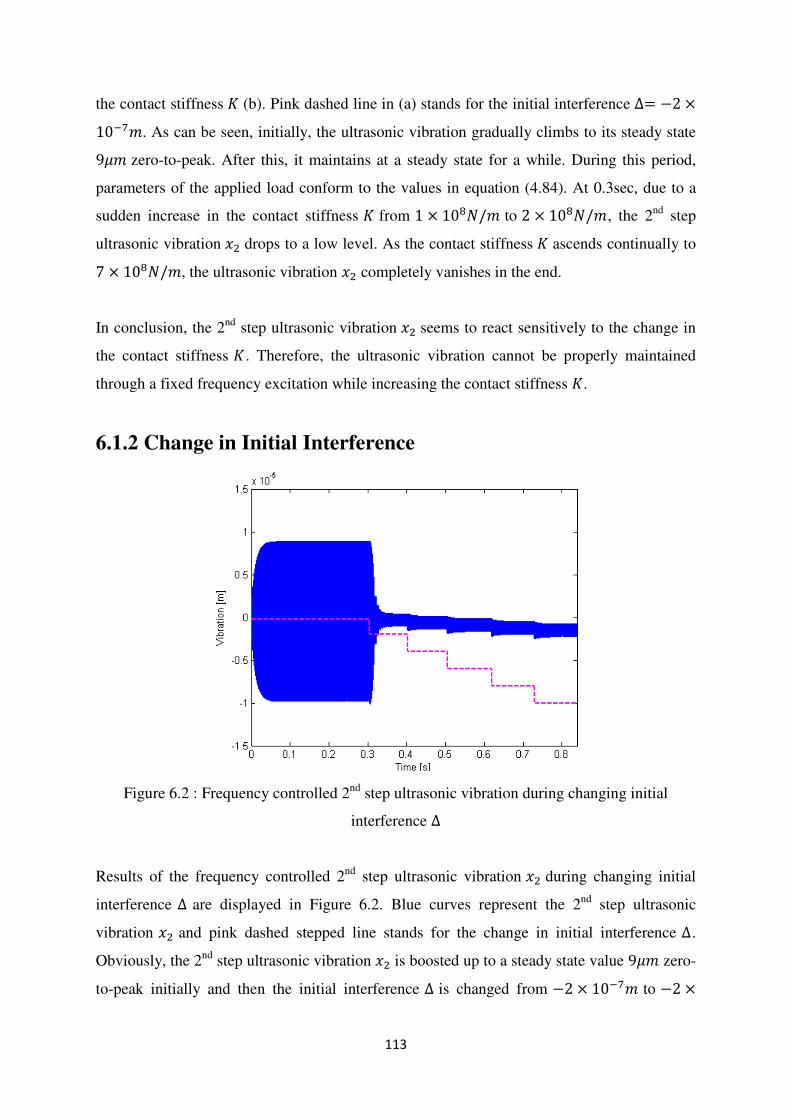
113
the contact stiffness � (b). Pink dashed line in (a) stands for the initial interference ∆= −2 ×
10−7�. As can be seen, initially, the ultrasonic vibration gradually climbs to its steady state
9�� zero-to-peak. After this, it maintains at a steady state for a while. During this period,
parameters of the applied load conform to the values in equation (4.84). At 0.3sec, due to a
sudden increase in the contact stiffness � from 1 × 10⁸�/� to 2 × 10⁸�/�, the 2nd
step
ultrasonic vibration �2 drops to a low level. As the contact stiffness � ascends continually to
7 × 10⁸�/�, the ultrasonic vibration �2 completely vanishes in the end.
In conclusion, the 2nd
step ultrasonic vibration �2 seems to react sensitively to the change in
the contact stiffness �. Therefore, the ultrasonic vibration cannot be properly maintained
through a fixed frequency excitation while increasing the contact stiffness �.
6.1.2 Change in Initial Interference
Figure 6.2 : Frequency controlled 2nd
step ultrasonic vibration during changing initial
interference ∆
Results of the frequency controlled 2nd
step ultrasonic vibration �2 during changing initial
interference ∆ are displayed in Figure 6.2. Blue curves represent the 2nd
step ultrasonic
vibration �2 and pink dashed stepped line stands for the change in initial interference ∆.
Obviously, the 2nd
step ultrasonic vibration �2 is boosted up to a steady state value 9�� zero-
to-peak initially and then the initial interference ∆ is changed from −2 × 10⁻⁷� to −2 ×

114
10−6� which leads to an essential decrease in the ultrasonic vibration magnitude at the end
of 2nd
step concentrator �2. As the initial interference ∆ keeps on increasing, the 2nd
step
ultrasonic vibration level �2 remains low. Another important notice is that the ultrasonic
vibration tends to shift downwards which is likely caused by the increase in the initial
engagement ∆ of the ultrasonic transducer into the applied load. Consequently, a fixed
frequency excitation on the ultrasonic transducer is not able to maintain the 2nd
step ultrasonic
vibration against the change in the initial interference ∆.
6.1.3 Conclusion
According to the simulation of a frequency controlled ultrasonic vibration, both change in the
contact stiffness � and in the initial interference ∆ have a significant impact on the ultrasonic
vibration at the end of 2nd
step concentrator �2. As parameters change, the 2nd
step ultrasonic
vibration �2 drops significantly. Hence, a robust control is strongly suggested to maintain the
2nd
step ultrasonic vibration �2 therefore autoresonance control has been developed.
6.2 Mechanical Feedback Control
Mechanical feedback uses the actual ultrasonic vibration at the end of 2nd
step concentrator �2 as feedback signal and aims at maintaining the ultrasonic vibration of 2nd
step �2 at a
desired level against the change in the contact stiffness � or the initial interference ∆ of the
applied load. Before mechanical feedback control is evaluated, a filter complementation on
the control system will be carried out.
6.2.1 Low-Pass Filter with a High Cut-Off Frequency
As introduced in Chapter Five that the filtering block in autoresonant control feedback
system plays a role in rectification (smoothing) of the amplified square wave in order to
generate a quasi-sine wave which eliminates the high frequency components. This quasi-sine
wave can be further supplied to the ultrasonic transducer to excite it and thus form the
feedback loop. Moreover, the filtering process can essentially eliminate a possible damage to
the piezorings due to high frequency noises. In other words, a properly designed filter is
required to cut off the high frequency components.

115
According to the amplitude-phase characteristic of observation point �2 shown in Figure
5.11, the curve is smooth and gently sloping near resonance. More importantly, the
characteristic of �2 is single-valued (one phase corresponds to one vibration magnitude)
which suggests a low-pass filter to the mechanical feedback in order to effectively get rid of
the high frequency noises. As is known to all, due to the frequency dependence property, a
filter involvement will inevitably introduce additional amplitude changes and phase shifts to
the original square wave (the square wave which has been operated by the phase shifter block
and the amplitude control block) which cannot be properly controlled by autoresonance.
Therefore, a properly designed filter is significant in feedback. After a careful consideration,
a first-order low-pass filter has been selected; a low-pass filter is a filter that passes low
frequency signals but attenuates (reduces the magnitude of) signals with frequencies higher
than the cut-off frequency. The transfer function of a first-order low-pass filter chosen for the
mechanical feedback system is obtained:
�(�) =10.000002�+1 (6.1)
Figure 6.3 : Amplitude-frequency characteristic of the low-pass filter
� is the Laplace operator. Time constant in this transfer function is � = 0.000002 therefore
the cut-off frequency in the amplitude-frequency characteristic of the transfer function shown
in equation (6.1) is � =1� = 500000���/� which equals 80���. Amplitude-frequency and
phase-frequency characteristics are illustrated in Figure 6.3 and Figure 6.4.

116
An interested frequency range to evaluate the low-pass filter has been selected � ∈[17���~25���] which centres on the ultrasonic transducer natural frequency shown in
equation (4.85). As can be seen in Figure 6.3, amplitude of the low-pass filter is kept roughly
at a constant level over a 8��� frequency range. To be exact, the gain that the feedback loop
is likely to benefit is around 0.965 which corresponds the resonant frequency (4.85) of the
ultrasonic vibrating system shown in Figure 4.17. As the contact stiffness � or the initial
interference ∆ increases, the resonant frequency of the ultrasonic vibrating system will shift.
However, maximal change in the resonant frequency is no more than 1��� (calculated
numerically) which according to Figure 6.3, the gain value of the low-pass filter hardly
changes. This is desirable for the autoresonant control design because the amplitude change
in the 2nd
step ultrasonic vibration �2 caused by the low-pass filter can be neglected.
Figure 6.4 : Phase-frequency characteristic of the low-pass filter
Phase-frequency characteristic of the low-pass filter (6.1) is displayed in Figure 6.4. This
characteristic is obtained in the same frequency range � ∈ [17���~25���] . It can be
observed that the phase shift introduced by the low-pass filter is insignificant. Phase change
due to the low-pass filter over the interested frequency range produce has a value −12~ − 17
degrees. Since change in the contact stiffness � or the initial interference ∆ will shift the
resonant frequency of the loaded ultrasonic transducer by no more than 1���, phase shift
introduced by the low-pass filter has a static value around −15 degrees. This value will not

117
essentially affect autoresonant control system because this is only a minor phase shift caused
by the low-pass filter.
Effectiveness of the low-pass filter smoothing the amplified square wave into a quasi-sin
wave has been examined and results are shown in Figure 6.5. Observing the input square
wave and the output quasi-sin wave, several conclusions can be drawn.
Figure 6.5 : Input and output of the low-pass filter: blue solid square wave – input to the low-
pass filter, red dashed curve – output from the low-pass filter
• The input signal and the output signal have a similar magnitude
• Output from the low-pass filter shows a minor phase shift and it will not drastically
affect the autoresonant control system
• Although the output signal is not a purely sine wave, it is still a workable actuation
signal in the feedback. On the other hand, the low-pass filter is able to reduce the high
frequency components which might cause serious damages to the piezorings.
Consequently, the selected low-pass filter has been applied to the mechanical feedback
control. In next section, amplitude-phase characteristic of the mechanical feedback system
will be presented before the control evaluation is examined because the autoresonant control
algorithm is based on phase control.

118
6.2.2 Amplitude-Phase Characteristic of Mechanical Feedback
Before mechanical feedback control is investigated, amplitude-phase characteristic of the
loaded ultrasonic transducer shown in Figure 4.17 should be obtained. To identify which
phase shift generates the optimal (maximal) vibration magnitude at the end of 2nd
step
concentrator �2, the phase has been slowly changed from a starting point and the peak values
of the ultrasonic vibration of 2nd
step concentrator �2 have been tracked literally. Amplitude-
phase characteristic of the mechanical feedback is shown in Figure 6.6.
Figure 6.6 : Amplitude-phase characteristic of the loaded ultrasonic transducer with
mechanical feedback control
It can be seen clearly, the curve is smooth and gently sloping near the peak which maps 0.2
phase control unit with a nearly 11�� zero-to-peak amplitude �2. It should be noted that 1
phase control unit equals 2�. Therefore the phase shift which gives the maximal ultrasonic
vibration magnitude is:
0.2 ∗ 2� = 0.4� (6.2)
Equation (6.2) indicates that by setting up a 0.4� phase shift between the 2nd
step ultrasonic
vibration �2 and the supplied voltage � to the ultrasonic transducer, the feedback is able to
tune itself at the most efficient state. Generally speaking, amplitude-phase characteristic
curve is reasonably flat around the resonance; hence amplitude will not change significantly

119
with a minor phase shift around the optimal value. In following sections, control evaluation
against the change in the contact stiffness � and the initial interference ∆ will be evaluated.
6.2.3 Change in Contact Stiffness
Mechanical feedback control aims at maintaining the ultrasonic vibration at the end of 2nd
step concentrator �2 at a constant level against the change in the applied load. The feedback
signal is the actual ultrasonic vibration of 2nd
step concentrator �2 . Mechanical feedback
employs �2 as an actuating signal and computes the RMS of �2 for each control cycle in
order to perform phase control and amplitude control according to the described amplitude-
phase control algorithm in section 5.1. Results are shown in Figure 6.7 during change in the
contact stiffness � in the applied load.
Figure 6.7 : Mechanical feedback during change in contact stiffness �: (a) RMS of the
feedback signal, (b) change in contact stiffness, (c) phase control, (d) amplitude control
Figure 6.7 (a) illustrates the RMS of the feedback signal �2 (black curve); pink dash-dotted
line illustrates the boundaries of the phase control zone, in this case, �� = 5%��. Red dotted
line represents the desired value of the ultrasonic vibration at the end of 2nd
step �2 in the
loaded ultrasonic transducer which has a notation ��. Since the displacement of 2nd
step �2 in
the loaded ultrasonic transducer has a value 9�� zero-to-peak, the desired RMS of �2 is

120
chosen to be �� ≈ 6.6��. Blue curve stands for the RMS of �2 calculated in infinite time
which has an equation:
��� = �1∞∫ �(�)2��∞0 (6.3)
In equation (6.3), RMS indicates the RMS value calculated in infinite time, �(�) is the sensor
signal. Figure 6.7 (b) depicts the change in contact stiffness �. Again, the range is � ∈ [1 ×
108�/� ~7 × 10⁸�/�] with an increment 1 × 10⁸�/�. (c) shows phase control and (d)
demonstrates amplitude control.
Operation procedure for the mechanical feedback control is: the closed loop of the
mechanical feedback with the ultrasonic vibration of 2nd
step �2 acting as the feedback signal
and the actuating signal. However, the 2nd
step ultrasonic vibration amplitude �2 shown in
Figure 6.6 presents a nearly 11�� zero-to-peak amplitude with an optimal phase shift 0.4�.
This mismatches the desired 9�� zero-to-peak which seems to be caused by the low-pass
filter. Therefore, the amplitude of the square wave has been adjusted to 170� zero-to-peak
which is further applied to the low-pass filter in order to generate a quasi-sin wave to drive
the ultrasonic transducer. Optimal phase shift 0.4� is set up initially in the closed loop. The
newly established 170� driving voltage produces a 9�� zero-to-peak vibration magnitude at
the end of 2nd
step in the closed loop. The RMS of the displacement at the end of 2nd
step �2
has been calculated for each control cycle. After the RMS signal stabilises, the combined
amplitude-phase algorithm will be applied. In this case, the stabilisation time for the RMS has
been explored as 5000 oscillation periods which equals around 0.25secs illustrated in Figure
6.7. The actual control cycle mentioned in equation (5.2) is chosen to be 200 oscillation
periods which equals around 0.01secs illustrated in Figure 6.7 (a) and (c). Control algorithm
is not executed until the steady state of the RMS is reached.
As can be seen clearly in Figure 6.7 that during the change in contact stiffness �, the RMS of
2nd
step vibration �2 for each control cycle does not leave phase control zone which gives rise
to no amplitude control participation shown in (d). This can be explained that the amplitude-
phase characteristic of the 2nd
step ultrasonic vibration �2 is reasonably flat around resonance.
In other words, the ultrasonic vibration of 2nd
step �2 can be controlled steadily by the phase

121
control algorithm which is demonstrated in (c). Obviously, change in the phase is about 0.06
phase control units starting from the optimal value 0.2 phase control units. Resonant
frequency of the loaded ultrasonic transducer with parameters in equation (4.84) is around
21.176��� which is calculated in equation (4.85). As the contact stiffness � changes, the
resonant frequency gradually shifts to 21.906��� when � = 7 × 10⁸�/�. In order to fully
understand the control effectiveness, the 2nd
step ultrasonic vibration �2 and the applied load
during change in the contact stiffness � are shown in Figure 6.8.
Figure 6.8 : Mechanical feedback controlled 2nd
step ultrasonic vibration during change in
contact stiffness �: (a) controlled ultrasonic vibration, (b) change in applied load, (c) change
in contact stiffness
Figure 6.8 (a) depicts ultrasonic vibration at the end of 2nd
step concentrator �2 while
changing the contact stiffness � of the applied load (c). The vibration signal seems stable
despite essential increase in the contact stiffness �. Another observation is the ultrasonic
vibration �2 tends to shift downwards as the increase in �; this is caused by the increase in
the applied load. (b) illustrates the applied load as the increase in the contact stiffness �.
Loading climbs up gradually from less than 1000� initially to nearly 5000� eventually.
Essential increase in the contact stiffness � imitates a promotion in the material (work piece)
elasticity. In spite of this, the mechanical feedback control is still capable of handling such a

122
drastic change and keeping the 2nd
step ultrasonic vibration �2 at a constant level. This
promising result implies the importance of a direct employment of the ultrasonic vibration as
a feedback signal and enhances the reliability and feasibility of the mechanical feedback
application.
Figure 6.9 is the enlarged picture of (a) in Figure 6.7. As can be seen, the black curve (RMS
of �2 for each control cycle) stays within the phase control zone (pink dash-dotted line)
which is kept closely to the desired RMS of the 2nd
step ultrasonic vibration �2 (shown in red-
dashed straight line). The maximum deviation of mechanical feedback in RMS of �2
monitoring from its desired �� = 6.6�� is around 0.3�� which equals 4%��.
Figure 6.9 : RMS of the 2nd
step ultrasonic vibration during change in contact stiffness �
6.2.4 Change in Initial Interference
Another parameter can also be changed to examine the efficiency of the mechanical feedback
is the initial interference ∆. It has been described that the change in ∆∈ [−2 × 10⁻⁷�~ −1 × 10⁻⁵�] with an increment −2 × 10⁻⁶� . Change in the initial interference ∆ will
inevitably shift the resonant frequency of the loaded ultrasonic transducer which according to
numerical calculation, resonant frequency shifts from 21.176��� to 21.188���. Results of
the mechanical feedback control during the change in initial interference ∆ are shown in
Figure 6.10.

123
Similarly, in Figure 6.10 (a) black curve is the RMS of �2 for each control cycle, blue curve
stands for the RMS of the 2nd
step ultrasonic vibration �2 calculated in infinite time, pink
dash-dotted lines define the upper and lower boundaries of the phase control zone which is
chosen to be �� = 5%�� , red dashed line is the desired RMS of the 2nd
step ultrasonic
vibration �2 that equals �� = 6.6��.
Figure 6.10 : Mechanical feedback during change in initial interference ∆: (a) RMS of the
feedback signal, (b) change in initial interference ∆, (c) phase control, (d) amplitude control
As can be seen, RMS of �2 (black curve) drops out of phase control zone a number of times,
which means by purely adjusting the phase is not able to keep the 2nd
step ultrasonic vibration �2 as a constant. Therefore, amplitude control has to be involved to inject more power into
the ultrasonic transducer in order to compensate the drop in the 2nd
step ultrasonic vibration �2 due to the change in the machining conditions (change in initial interference ∆ ).
Amplitude control has been showed in (d). Amplitude of the square wave has been increased
from initial 170� to nearly 260� when the initial interference changes from −2 × 10⁻⁷� to −1 × 10⁻⁵� illustrated in (b). Phase control in this case increases from 0.2 phase control
units to 0.27 phase control units. For the change in the initial interference ∆, algorithm of the

124
combined amplitude-phase algorithm has been employed to maintain the 2nd
step ultrasonic
vibration �2.
Figure 6.11 illustrates the mechanical feedback controlled ultrasonic vibration of 2nd
step
concentrator �2 and applied load during the change in the initial interference ∆. As can be
seen in (a) that the 2nd
step ultrasonic vibration �2 can be generally kept at a constant level
during change in the initial interference ∆ (pink dashed line). Similar to the case of change in
the contact stiffness � , controlled ultrasonic vibration presents a shifting downwards
characteristic because of the change in the initial interference ∆. Physically it means an
increase engagement of a tool into the target work piece. Applied load increases from initial
1000� to more than 1500� in the end which is essentially smaller than the applied load
increase in the case of change in the contact stiffness �.
Figure 6.11 : Mechanical feedback controlled 2nd
step ultrasonic vibration during change in
initial interference ∆: (a) controlled ultrasonic vibration, (b) change in applied load
Figure 6.12 is the enlarged picture of (a) in Figure 6.10. As can be seen, the RMS of �2 drops
out of phase control zone a number of times which suggests an amplitude control
participation. As a result, an extra power supply provided by the amplitude control
automatically restores the RMS of 2nd
step ultrasonic vibration �2 to the desired level ��. The

125
maximal deflection of RMS of �2 from its desired �� against change in the initial
interference ∆ is about 0.4�� that equals 6%��. Results presented above prove autoresonant
control is able to cope with the change in the initial interference ∆ with a combined
amplitude-phase control algorithm.
Figure 6.12 : RMS of the 2nd
step ultrasonic vibration during change in initial interference ∆
6.2.5 Conclusion
In conclusion, mechanical feedback control is capable of maintaining the ultrasonic vibration
of the 2nd
step concentrator �2 at a constant level. In the case of change in the contact
stiffness �, phase control algorithm suffices to keep the 2nd
step ultrasonic vibration �2 at a
desired level. Maximal deflection of the RMS of the ultrasonic vibration �2 is 0.3�� which
equals 4%�� . In contrast, change in the initial interference ∆ in the applied load model
requires a combined amplitude-phase control algorithm for the loaded ultrasonic transducer
to acquire more power to keep the ultrasonic vibration of 2nd
step �2 at a constant. Deviation
of RMS of �2 in change in the initial interference ∆ is 0.4�� equals 6%��.
In next section, electrical feedback control will be evaluated. Basically, electrical feedback
control consists of two strategies which are current feedback control and power feedback
control. Filter design is introduced before the control efficiency is evaluated. The influence of
different bandwidth of filters selection on the autoresonant control will be investigated.

126
Electrical feedback will also be tested on the change in the contact stiffness � ∈[1 × 10⁸�/�~7 × 108�/�] with an increment 1 × 10⁸�/� and the change in the initial
interference ∆∈ [−2 × 10⁻⁷�~− 1 × 10⁻⁵�] with an increment −2 × 10⁻⁶�.
6.3 Current Feedback Control
In this section, current feedback control will be examined during the change in the contact
stiffness � and the change in the initial interference ∆. Before the autoresonant control on the
current feedback is examined, filters design will be carried out. As analysed in Figure 5.11 in
section 5.3.3 that the amplitude-phase characteristic displays an ambiguity property when the
1st step concentrator vibration �1 is chosen to be the observation point. Therefore, it is
strongly suggested a filtration process participation into the feedback. In other words, in the
amplitude-phase characteristic, one phase shift reflects several vibration magnitudes which
will inevitably bring ‘confusion’ to feedback when the current � is selected to be the feedback
signal. Hence, a band-pass filter is recommended to pick up the wanted vibration regimes. In
addition, in order to check the filter bandwidth effect on the autoresonant control, several
bandwidths will be applied to rectify the amplified square wave signal in the current
feedback.
Current feedback control uses the current � as both a feedback signal and an actuation signal.
The target of the current feedback control is to maintain the 2nd
step ultrasonic vibration �2
through stabilising current during the change in the applied load. Current feedback control is
an indirect control method compared with mechanical feedback control, so the control is
expected to be not efficient as mechanical feedback control.
Recalling the expressions of the current of the piezoelectric transducer shown in equation
(5.18) has the following form:
� = �̇ = �03�̇0 + �04�̇ (6.4)
Where �03 = 3.4 × 10⁻¹⁰ and �04 = 2.1 × 10⁻⁹ are coefficients shown in equation (4.63), �
is the charge, � is the supplied voltage and �0 is the interaction force between a piezoring and
the 1st step concentrator. The expression of �0 and �0 are shown in the following:

127
�0 =1�01 �0 + �02� (6.5)
�0 = �1(�̇1 − �̇0) + �1(�1 − �0) (6.6)
Where �01 and �02 are parameters shown in equation (4.63) and �1 and �1 are parameters
shown in equation (4.59) and (4.75).
6.3.1 Band-Pass Filter Design
As described in Figure 5.11 that the amplitude-phase characteristic is ambiguous when the 1st
step ultrasonic vibration �1 is the observation point which suggests a band-pass filter
participation to filter out the desired oscillation regime. After several types of band-pass filter
investigations, a 2nd
order Butterworth filter has been eventually employed. A Butterworth
filter is a type of signal processing filter designed to have as flat a frequency response as
possible in the pass-band which also refers to as a maximally flat magnitude filter. Ideally, a
filter should not only completely reject the unwanted frequencies but should also have an
uniform sensitivity for the wanted frequencies.
The frequency response of a Butterworth filter is maximally flat (i.e. has no ripples) in the
pass-band and rolls off towards zero in the stop-band. Figure 5.11 shows 3 possible
oscillation regimes when the 1st step concentrator ultrasonic vibration �1 is selected to be the
observation point. Each of the 3 oscillation regimes reflects a different amplitude-frequency
characteristic. Consequently, by choosing a proper bandwidth for a Butterworth filter allows
the desired oscillation regime to be kept while the other 2 are rejected. Due to the fact that
during change in the contact stiffness � of the applied load, the resonant frequency shifts
from 21.176��� to 21.906���, the bandwidth of a Butterworth filter has been selected to
centre around 21.54��� consequently. 3 bandwidths of the Butterworth filters have been
chosen which are 19.54���~23.54��� corresponds to a 4���
bandwidth, 17.54���~25.54��� corresponds to a 8��� bandwidth and
15.54���~27.54��� corresponds to a 12��� bandwidth. These 3 filters bandwidths
centre on 21.54��� . The frequency range used to calculate the characteristics of the
Butterworth filters is selected � ∈ [12���~30�ℎ�]. The transfer functions for the 4���,
8���, and 12��� Butterworth filters are:

128
�4��� =6.317×10⁸�2�4+3.554×10⁴�3+3.695×10¹⁰�2+6.454×10¹⁴�+3.297×10²⁰ (6.7)
�8��� =2.527×10⁹�2−2.739×10⁻¹⁰�−398.8�4+7.109×10⁴�3+3.79×10¹⁰�2+1.257×10¹⁵�+3.128×10²⁰ (6.8)
�12��� =5.685×10⁹�2−3.082×10⁻¹⁰�−566.3�4+1.066×10⁵�3+3.948×10¹⁰�2+1.802×10¹⁵�+2.855×10²⁰ (6.9)
Figure 6.13 demonstrates the amplitude-frequency characteristics for 3 bandwidths
Butterworth filters. Blue solid curve represents a 4��� bandwidth Butterworth filter, red
dashed curve stands for a 8��� bandwidth Butterworth filter and green dash-dotted curve
shows a 12��� bandwidth Butterworth filter. As can be seen clearly, 3 Butterworth filters
have a flat magnitude response within their own pass-band. In contrast, for those frequencies
beyond the pass-band, magnitude response falls quickly to a low level. Theoretically, a wider
bandwidth in a Butterworth filter is advised to participate in the feedback since it provides a
wider range of flat magnitude response. This provides the loaded ultrasonic transducer with
more freedom to adapt itself in order to deal with the change in the applied load.
Figure 6.13 : Amplitude-frequency characteristic of 3 bandwidths Butterworth filters: blue
solid curve – 4��� bandwidth, red dashed curve - 8��� bandwidth, green dash-dotted curve
- 12��� bandwidth

129
Phase-frequency characteristics of 3 bandwidths Butterworth filters are shown in Figure 6.14.
Blue solid curve means a 4��� bandwidth Butterworth filter, red dashed curve stands for a
8��� bandwidth Butterworth filter and green dash-dotted curve shows a 12��� bandwidth
Butterworth filter. Clearly, a narrower band Butterworth filter presents a more drastic change
in phase compared with a wider one. The phase shift introduced by the filter is uncontrollable
by the phase control algorithm. As can be seen, the phase shift for a 4��� Butterworth filter
equals 140~− 140 degrees, the phase shift for a 8��� and a 12��� Butterworth filter have
a similar phase shift within their corresponding pass-band. However, the slopes of the 8���
and the 12��� Butterworth filters are much gentler in comparison with the slope of the
4��� Butterworth filter. Generally, the change in phase caused by the filter needs to be small
around the operation frequency. A conclusion hence can be pre-drawn that a 8��� and a
12��� Butterworth filters are supposed to be more efficient than a 4��� Butterworth filter.
Figure 6.14 : Phase-frequency characteristic of 3 bandwidths Butterworth filters: blue solid
curve – 4��� bandwidth, red dashed curve - 8��� bandwidth, green dash-dotted curve -
12��� bandwidth
Smoothed square waves by 3 bandwidths Butterworth filters have been shown in Figure 6.15.
Blue square wave represents the amplified input signal into the 2nd
order Butterworth filters,
red curve is the output from a 4��� bandwidth Butterworth filter, green dashed curve stands
for the output from a 8��� bandwidth Butterworth filter and pink dash-dotted curve
indicates the output from a 12��� bandwidth Butterworth filter. As can be seen, the square

130
wave has been smoothed by 3 Butterworth filters at a frequency 21.176��� which is the
resonant frequency of the loaded ultrasonic transducer with parameters shown in equation
(4.85). Phase shifts of the generated sinusoidal waves reflect the 21.176��� corresponded
phase values in Figure 6.14 for 3 Butterworth filters. Another notable point in Figure 6.15 is
that each of the filtered sinusoidal wave signals has enlarged amplitudes than the amplitude
of the square wave. However, according to Figure 6.13, the gain of the Butterworth filters
within the pass-band is unity. This seems controversial. However, the amplification is
because a Butterworth filter only takes the 1st harmonic frequency corresponded component
which is always larger than the amplitude of the square wave. The 2nd
, 3rd
and higher order of
harmonic frequency components have been effectively removed by the Butterworth filters.
Figure 6.15 : Input and output of the 2nd
order Butterworth filters: blue square wave – input to
the filters, red curve – output from a 4��� filter, green dashed curve – output from a 8���
filter, pink dash-dotted curve – output from a 12��� filter
6.3.2 Amplitude-Phase Characteristics of Current and 2nd
step
Ultrasonic Vibration
Equation (6.4) shows the current calculation which will be used to form the current feedback.
The current � is related to both the interaction force �0 between a piezoring and the 1st step
concentrator and the supplied voltage �. Current � has been used as both the feedback signal
and the actuation signal.

131
This section is dedicated to the investigation of autoresonance control of the current feedback
with 3 bandwidths Butterworth filters applications. Results are compared and analysed.
Control evaluation is carried out on the change in the contact stiffness � and the change in
the initial interference ∆ of the applied load model described in Figure 4.17. Before the
control is evaluated, the amplitude-phase characteristics of the current feedback for both the
current � and the 2nd
step ultrasonic vibration �2 for 3 Butterworth filters need to be obtained.
Since the current feedback relies on the amplitude-phase characteristic of the current � flows
through the piezoelectric transducer as it acts as both the feedback signal and the actuation
signal, it is sensible to obtain the amplitude-phase characteristic of the current � initially.
Meanwhile, it is worth to draw the amplitude-phase characteristic of the 2nd
step ultrasonic
vibration �2.
Operation procedure of this process is that the loop is closed in the beginning and the phase
shift is slowly changed with an increment 0.01 phase control unit between the current � and
the supplied voltage �. Both current � and the 2nd
step ultrasonic vibration �2 is recorded
accordingly. It should be noted that there are 3 Butterworth filters with 4�� ,8��� and
12��� bandwidths respectively. These filters will be applied to the current feedback
literally. Therefore, 3 amplitude-phase characteristics for the current � and 3 characteristics
for the 2nd
step ultrasonic vibration �2 are obtained.
6.3.2.1 Amplitude-Phase Characteristics of a ���� Butterworth
Filter
Figure 6.16 illustrates the current amplitude-phase characteristic of the loaded ultrasonic
transducer with a 4��� bandwidth Butterworth filter application. As can be seen, when the
phase shift between the current � and the supplied voltage � is 0.08 phase control units which
equals 0.16�, the optimal regime for current feedback is reached with a peak value 0.323�
zero-to-peak. Physically, it indicates by setting up a 0.16� phase shift in the feedback loop
allows the current to tune itself at the most efficient state.
Figure 6.17 demonstrates the amplitude-phase characteristic of the 2
nd step ultrasonic
vibration �2 with a 4��� bandwidth Butterworth filter application. It can be observed that a
0.05 phase shift equivalently 0.1� ensures the 2nd
step ultrasonic vibration �2 to have a

132
resonant regime with an amplitude 11.93�� zero-to-peak. Due to the Butterworth filter
effect, a 0.08 phase shift corresponded ultrasonic vibration amplitude also has a mismatch
with desired amplitude 9�� zero-to-peak. Therefore, the supplied voltage � has been tuned
in order to match the 2nd
step ultrasonic vibration amplitude 9�� zero-to-peak at resonance.
As a result, optimal phase shift with an application of a 4��� bandwidth Butterworth filter in
the current feedback control is tuned to be 0.16�.
Figure 6.16 : Current amplitude-phase characteristic of the loaded ultrasonic transducer
Figure 6.17 : 2nd
step ultrasonic vibration amplitude-phase characteristic of the loaded
ultrasonic transducer

133
6.3.2.2 Amplitude-Phase Characteristics of a ���� Butterworth
Filter
Figure 6.18 : Current amplitude-phase characteristic of the loaded ultrasonic transducer
Figure 6.19 : 2nd
step ultrasonic vibration amplitude-phase characteristic of the loaded
ultrasonic transducer
Figure 6.18 presents the current amplitude-phase characteristic of the loaded ultrasonic
transducer with a 8��� bandwidth Butterworth filter application. The 8��� Butterworth
filter enables the current feedback to reach its resonant state at a phase shift 0.05 phase

134
control units which equals 0.1� . In other words, the current � has a maximal amplitude
0.323� zero-to-peak with a phase shift 0.1�.
Figure 6.19 depicts the 2nd
step ultrasonic vibration �2 amplitude-phase characteristic with a
8��� bandwidth Butterworth filter application. Clearly, a phase shift 0.05 phase control unit
( 0.1� ) permits the 2nd
step ultrasonic vibration �2 to reach its resonant state with an
amplitude 11.59�� zero-to-peak. Therefore, for a 8��� bandwidth Butterworth filter
application, phase shift has been tuned as 0.1� to guarantee the ultrasonic transducer to reach
the current resonant regime. Again, due to the Butterworth filter effect, the supplied voltage �
will be adjusted to conform to the ultrasonic vibration amplitude at the end of the 2nd
step of
the loaded ultrasonic transducer to be 9�� zero-to-peak at the resonant state.
6.3.2.3 Amplitude-Phase Characteristics of a �����
Butterworth Filter
Figure 6.20 : Current amplitude-phase characteristic of the loaded ultrasonic transducer
The amplitude-phase characteristics of the current � and the 2nd
step ultrasonic vibration �2
with a 12��� bandwidth Butterworth filter application are illustrated in Figure 6.20 and
Figure 6.21. In Figure 6.20, it indicates that the current � arrives at its resonant state with a
phase shift 0.06 phase control units (0.12�) and amplitude of current is 0.319� zero-to-peak.
Figure 6.21 implies that a shift of 0.05 phase control units (0.1� ) permits the 2nd
step
ultrasonic vibration �2 to reach its resonant state with an amplitude 11�� zero-to-peak. The

135
supplied voltage � has to be adjusted in order to match the desired 2nd
step ultrasonic
vibration amplitude 9�� zero-to-peak.
Figure 6.21 : 2nd
step ultrasonic vibration amplitude-phase characteristic of the loaded
ultrasonic transducer
As a result, the optimal phase shift value for the current feedback control system for 3
bandwidths Butterworth filters are obtained respectively. Simultaneously, current feedback
controlled 2nd
step ultrasonic vibration optimal phase shift values are also calculated. These
optimal phase shift values are shown in Table 6.1. As can be seen, the peak response of the
2nd
step ultrasonic vibration �2 with current feedback control seems to be achieved with a
fixed phase shift 0.1� despite the change in the bandwidth in Butterworth filters. Another
notable point is that only the 8��� bandwidth Butterworth filter generates a coincidence
phase shift between the current � and the 2nd
step ultrasonic vibration �2.
Table 6.1 : Optimal phase shift values of the current and the 2nd
step ultrasonic vibration for 3
bandwidths Butterworth filters
Bandwidth
Optimal Ph.Shift
4��� 8��� 12���
Current 0.16� 0.1� 0.12�
2nd
step ultrasonic vibration 0.1� 0.1� 0.1�

136
In next section, these optimal phase shifts will be applied to the current feedback control on
the loaded ultrasonic transducer model in Matlab-Simulink. Before the current feedback is
evaluated, amplitude of the square wave of the supplied voltage � should be computed in
order to match the 2nd
step ultrasonic vibration amplitude 9�� zero-to-peak for 3 bandwidths
Butterworth filters. The adjusted voltage amplitudes are shown in Table 6.2.
Table 6.2 : Square wave voltage amplitude for three bandwidths Butterworth filters
Bandwidth 4��� 8��� 12���
Voltage amplitude (V) 170 170 183
6.3.3 Change in Contact Stiffness
6.3.3.1 A ���� Butterworth Filter
For a 4��� bandwidth Butterworth filter application in the current feedback, the supplied
voltage amplitude of the square wave is around 170� zero-to-peak shown in Table 6.2.
Therefore, the corresponding current amplitude can be calculated by applying the phase shift
0.16� shown in Table 6.1 to the feedback loop. The desired RMS of current � hence is 0.18�
which produces the RMS of the 2nd
step ultrasonic vibration �2 6.6��. The current feedback
control results are shown in Figure 6.22.
(a) represents the RMS of the current for each control cycle (200 oscillation periods, same as
the mechanical feedback) shown in black line. Blue curve is the current RMS calculated in
infinite time. Red dashed straight line represents the desired RMS of the current which is �� = 0.18� and pink dash-dotted lines are the boundaries of the phase control zone. In this
case, �� = 10%�� . (b) demonstrates the increase in the contact stiffness � in the applied
load and the range is � ∈ [1 × 10⁸�/� ~7 × 10⁸�/�] . (c) indicates the phase control
during the change in the contact stiffness � and it conforms to the phase control algorithm.
(d) is amplitude control which follows the amplitude control algorithm. As can be seen, RMS
of the feedback signal (current) does not leave the phase control zone (pink dash-dotted line).
Therefore, no change is witnessed in the amplitude control and it is kept as a constant 170�.
For phase control, the value generally decreases from 0.08 phase control units to almost 0.01
phase control unit despite some fluctuations during the change in the contact stiffness �. This
is caused by the additional phase shift introduced by a 4��� Butterworth filter as can be
observed in phase-frequency characteristic in Figure 6.14. The resonant frequency of the

137
loaded ultrasonic transducer shifts from 21.176��� to 21.906��� due to the change in the
contact stiffness � which inevitably gives rise to a considerable phase shift in the Butterworth
filter. A narrow bandwidth Butterworth filter exhibits a relatively drastic phase shift
compared to a wider bandwidth Butterworth filter.
Figure 6.22 : Current feedback during changing contact stiffness: (a) RMS of feedback signal
(current), (b) change in contact stiffness, (c) phase control, (d) amplitude control
Figure 6.23 shows the controlled current during the change in the contact stiffness �. As can
be seen in (a), current remains stable during the change in � (b) despite some moderate drops
and ripples. However, the target of the current feedback is to maintain the ultrasonic vibration
of 2nd
step concentrator �2 as a constant by keeping the current signal stable. Hence, it is
advisable to evaluate the control of 2nd
step ultrasonic vibration �2.
Figure 6.24 demonstrates the current feedback controlled ultrasonic vibration of 2nd
step
concentrator �2 with a 4��� bandwidth Butterworth filter application. As can be seen in (a),
the 2nd
step ultrasonic vibration �2 is kept at a stable level during the change in the contact
stiffness � (c). Applied load (b) increases essentially from 1000� to nearly 5000� . Red
dashed line in (a) represents the initial interference ∆= −2 × 10⁻⁷�. Generally speaking, the
2nd
step ultrasonic vibration �2 tends to shift downwards which has been observed also in the

138
mechanical feedback control. This is caused by a significant increase in the contact stiffness � . A difficult-to-engage into the material due to the elasticity increase produces certain
asymmetry in the 2nd
step ultrasonic vibration �2.
Figure 6.23 : Current feedback controlled current during changing contact stiffness �: (a)
controlled current, (b) change in contact stiffness
Figure 6.24 : Current feedback controlled 2nd
step ultrasonic vibration during change in
contact stiffness �: (a) controlled ultrasonic vibration, (b) change in applied load, (c) change
in contact stiffness

139
Figure 6.25 depicts the RMS of the current � and the 2nd
step ultrasonic vibration �2
respectively. (a) is the enlarged image of (a) in Figure 6.22. As can be seen, only phase
control algorithm is applied during the change in the contact stiffness � due to the fact that
the RMS of feedback signal (current) does not leave the phase control zone. (b) demonstrates
the RMS of the 2nd
step ultrasonic vibration �2 for each control cycle (black curve). The
maximal deviation of the RMS of the 2nd
step ultrasonic vibration �2 from the desired level �� = 6.6�� is around 0.7�� which equals 11%��. To this point, current feedback with an
application of a 4��� bandwidth Butterworth filter during the change in the contact stiffness � seems inferior than the mechanical feedback control which only has a RMS 0.3��
(4%��) deflection. In next section, a 8��� bandwidth Butterworth filter application on the
current feedback during the change in the contact stiffness � will be carried out.
Figure 6.25 : (a) RMS of current, (b) RMS of 2nd
step ultrasonic vibration
6.3.3.2 A ���� Butterworth Filter
For a 8��� bandwidth Butterworth filter application in the current feedback, the supplied
voltage amplitude is also170� zero-to-peak shown in Table 6.2. The desired RMS of the
current is 0.18� which generates RMS of the 2nd
step ultrasonic vibration 6.6��. In Figure
6.26, (a) represents the RMS of the current � for each control cycle (200 oscillation periods,
same as the mechanical feedback) shown in black line. Blue curve is the current RMS

140
calculated in infinite time. Red dashed straight line represents the desired RMS of the current � which is �� = 0.18� and pink dash-dotted boundaries are the phase control zone. In this
case, �� = 10%�� . (b) demonstrates the increase in the contact stiffness � in the applied
load and the range is � ∈ [1 × 10⁸�/� ~7 × 10⁸�/�]. (c) is the phase control during the
change in the contact stiffness � and it conforms to the phase control algorithm. (d) is the
amplitude control which follows the amplitude control algorithm. As can be seen, RMS of the
feedback signal (current) does not leave the phase control zone (pink dash-dotted line) which
leads to no changes in the amplitude control. For phase control, the value generally decreases
from 0.05 phase control units to 0.03 phase control unit. Compared with a 4��� Butterworth
filter application, a 8��� filter effect on the phase shift seems much alleviated because of an
increased bandwidth.
Figure 6.26 : Current feedback during change in contact stiffness �: (a) RMS of the feedback
signal (current), (b) change in contact stiffness, (c) phase control, (d) amplitude control
Figure 6.27 shows the controlled current during the change in the contact stiffness �. As can
be seen in (a) that the current remains stable during the change in the contact stiffness (b).
This is similar to a 4��� bandwidth Butterworth filter application. Nonetheless, the aim of
the current feedback is to keep the 2nd
step ultrasonic vibration �2 at a constant level by

141
maintaining current � steady. Consequently, it is important to examine the control of the 2nd
step ultrasonic vibration �2.
Figure 6.27 : Current feedback controlled current during change in contact stiffness �: (a)
controlled current, (b) change in contact stiffness
Figure 6.28 shows the current feedback controlled ultrasonic vibration of 2nd
step
concentrator �2 with a 8��� bandwidth Butterworth filter application. As can be seen in (a),
being similar to the 4��� filter application case, the 2nd
step ultrasonic vibration �2 is kept at
a stable level during the change in the contact stiffness � (c). Applied load (b) increases
considerably from 1000� to nearly 5000� . Red dashed line represents the initial
interference ∆= −2 × 10⁻⁷� . Again, the 2nd
step ultrasonic vibration �2 tends to shift
downwards which is caused by a significant increase in the contact stiffness �.
Figure 6.29 depicts the RMS of the current � and the 2nd
step ultrasonic vibration �2. (a) is the
enlarged picture of (a) in Figure 6.26. (b) demonstrates the RMS of the 2nd
step ultrasonic
vibration �2 for each control cycle (black curve). According to the simulation results,
maximal deflection in RMS of the 2nd
step ultrasonic vibration �2 from the desired value �� = 6.6�� is around 0.5�� that equals 8%�� . To this point, the current feedback with
application of a 8��� bandwidth Butterworth filter during the change in the contact stiffness

142
� seems slightly worse than the mechanical feedback which only has a RMS 0.3�� (4%��)
deviation. However, the application of a 8��� bandwidth Butterworth filter in current
feedback still demonstrates certain improvement from a 4��� bandwidth Butterworth filter
which has a 0.7�� that equals 11%�� . In next section, a 12��� bandwidth Butterworth
filter application during the change in contact stiffness � will be examined.
Figure 6.28 : Current feedback controlled 2nd
step ultrasonic vibration during change in
contact stiffness �: (a) controlled ultrasonic vibration, (b) change in applied load, (c) change
in contact stiffness
Figure 6.29 : (a) RMS of current, (b) RMS of 2nd
step ultrasonic vibration
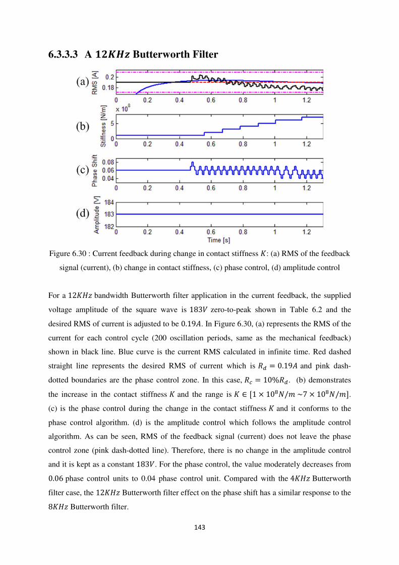
143
6.3.3.3 A ����� Butterworth Filter
Figure 6.30 : Current feedback during change in contact stiffness �: (a) RMS of the feedback
signal (current), (b) change in contact stiffness, (c) phase control, (d) amplitude control
For a 12��� bandwidth Butterworth filter application in the current feedback, the supplied
voltage amplitude of the square wave is 183� zero-to-peak shown in Table 6.2 and the
desired RMS of current is adjusted to be 0.19�. In Figure 6.30, (a) represents the RMS of the
current for each control cycle (200 oscillation periods, same as the mechanical feedback)
shown in black line. Blue curve is the current RMS calculated in infinite time. Red dashed
straight line represents the desired RMS of current which is �� = 0.19� and pink dash-
dotted boundaries are the phase control zone. In this case, �� = 10%��. (b) demonstrates
the increase in the contact stiffness � and the range is � ∈ [1 × 10⁸�/� ~7 × 10⁸�/�].
(c) is the phase control during the change in the contact stiffness � and it conforms to the
phase control algorithm. (d) is the amplitude control which follows the amplitude control
algorithm. As can be seen, RMS of the feedback signal (current) does not leave the phase
control zone (pink dash-dotted line). Therefore, there is no change in the amplitude control
and it is kept as a constant 183�. For the phase control, the value moderately decreases from
0.06 phase control units to 0.04 phase control unit. Compared with the 4��� Butterworth
filter case, the 12��� Butterworth filter effect on the phase shift has a similar response to the
8��� Butterworth filter.

144
Figure 6.31 : Current feedback controlled current during change in contact stiffness �: (a)
controlled current, (b) change in contact stiffness
Figure 6.32 : Current feedback controlled 2nd
step ultrasonic vibration during change in
contact stiffness �: (a) controlled ultrasonic vibration, (b) change in applied load, (c) change
in contact stiffness
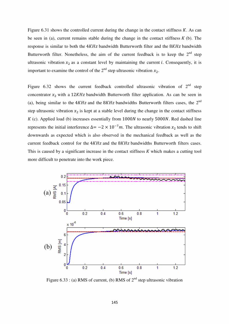
145
Figure 6.31 shows the controlled current during the change in the contact stiffness �. As can
be seen in (a), current remains stable during the change in the contact stiffness � (b). The
response is similar to both the 4��� bandwidth Butterworth filter and the 8��� bandwidth
Butterworth filter. Nonetheless, the aim of the current feedback is to keep the 2nd
step
ultrasonic vibration �2 as a constant level by maintaining the current �. Consequently, it is
important to examine the control of the 2nd
step ultrasonic vibration �2.
Figure 6.32 shows the current feedback controlled ultrasonic vibration of 2nd
step
concentrator �2 with a 12��� bandwidth Butterworth filter application. As can be seen in
(a), being similar to the 4��� and the 8��� bandwidths Butterworth filters cases, the 2nd
step ultrasonic vibration �2 is kept at a stable level during the change in the contact stiffness � (c). Applied load (b) increases essentially from 1000� to nearly 5000�. Red dashed line
represents the initial interference ∆= −2 × 10⁻⁷�. The ultrasonic vibration �2 tends to shift
downwards as expected which is also observed in the mechanical feedback as well as the
current feedback control for the 4��� and the 8��� bandwidths Butterworth filters cases.
This is caused by a significant increase in the contact stiffness � which makes a cutting tool
more difficult to penetrate into the work piece.
Figure 6.33 : (a) RMS of current, (b) RMS of 2nd
step ultrasonic vibration

146
Figure 6.33 depicts the RMS of the current � and the 2nd
step ultrasonic vibration �2. (a) is the
enlarged picture of (a) in Figure 6.30. As can be seen, phase control is able to keep the
current � as a constant during the change in the contact stiffness �. (b) demonstrates the RMS
of the 2nd
step ultrasonic vibration �2 for each control cycle (black curve). Maximal
deflection of the RMS of the 2nd
step ultrasonic vibration �2 from the desired value �� =
6.6�� is around 0.5�� which equals 8%��. To this point, a 12��� bandwidth Butterworth
filter application in the current feedback control during the change in the contact stiffness �
seems worse than the mechanical feedback which only has a RMS 0.3�� (4%��) deviation.
However, the performance of a 12��� bandwidth Butterworth filter application is still better
than the 4��� bandwidth Butterworth filter application which has a deviation 0.7��
(11%��) and is similar to the 8��� bandwidth Butterworth filter application which has a
deflection 0.5�� (8%��). In next section, current feedback control during the change in the
initial interference ∆ for 3 bandwidths Butterworth filters will be examined and compared.
6.3.4 Change in Initial Interference
6.3.4.1 A ���� Butterworth Filter
For a 4��� bandwidth Butterworth filter application in the current feedback, the supplied
voltage amplitude is around 170� zero-to-peak, the desired RMS of current hence is 0.18�
and the optimal phase shift is 0.16� initially which is same as the case of the 4���
Butterworth filter during the change in the contact stiffness �. In Figure 6.34, (a) represents
the RMS of the current for each control cycle (200 oscillation periods, same as the
mechanical feedback) shown in black line. Blue curve is the current RMS calculated in
infinite time. Red dashed straight line represents the desired RMS of the current which is �� = 0.18� and pink dash-dotted boundaries are the phase control zone. In this case, �� = 10%��. (b) demonstrates the increase in the initial interference ∆ in the applied load
and the range is ∆∈ [−2 × 10⁻⁷� ~− 1 × 10⁻⁵�] . (c) is the phase control during the
change in the initial interference ∆ and it conforms to the phase control algorithm. (d) is the
amplitude control and it conforms to the amplitude control algorithm. As can be seen, RMS
of the feedback signal (current) leaves phase control zone (pink dash-dotted line) several
times which causes increase in the amplitude control to nearly 220� eventually. For phase
control, the value generally decreases from 0.08 phase control units to almost 0.04 phase
control unit which seems less drastic compared with the change in the contact stiffness �.

147
This is because the increase in the initial interference ∆ shifts the resonant frequency of the
loaded ultrasonic transducer only from 21.176��� to 21.188���.
Figure 6.34 : Current feedback during change in initial interference ∆: (a) RMS of feedback
signal (current), (b) change in initial interference, (c) phase control, (d) amplitude control
Figure 6.35 shows the controlled current during the change in the initial interference ∆. As
can be seen in (a), current remains stable during the change in the initial interference ∆ (b)
even though some increases have been detected because of extra supplied voltage. However,
the target of the current feedback is to maintain the ultrasonic vibration of 2nd
step
concentrator �2 at a constant level by keeping current � stable. Therefore, it is important to
evaluate the control of 2nd
step ultrasonic vibration �2.
Figure 6.36 demonstrates the current feedback controlled 2nd
step ultrasonic vibration �2 with
a 4��� bandwidth Butterworth filter application. As can be seen in (a), the 2nd
step
ultrasonic vibration �2 is kept at a stable level during the change in the initial interference ∆
shown in pink dashed line. Applied load (b) increases from 1000� to nearly 1500� .
Generally speaking, the 2nd
step ultrasonic vibration �2 fluctuates around the desired level
with the help of the amplitude control.

148
Figure 6.35 : Current feedback controlled current during change in initial interference ∆: (a)
controlled current, (b) change in initial interference
Figure 6.36 : Current feedback controlled 2nd
step ultrasonic vibration during change in initial
interference ∆: (a) controlled ultrasonic vibration, (b) change in nonlinear loading
Figure 6.37 depicts the RMS of the current and the ultrasonic vibration of 2nd
step
concentrator. (a) is the enlarged picture of (a) in Figure 6.34. Amplitude-phase combined

149
control algorithm has been applied during the current feedback control as a result of the RMS
dropping out of the phase control zone. (b) demonstrates the RMS of the ultrasonic vibration
of 2nd
step concentrator �2 for each control cycle (black curve). Maximal deflection of the
RMS of the 2nd
step ultrasonic vibration �2 from the desired value �� = 6.6�� is around
0.8�� which equals 12%�� . To this point, the current feedback with an application of a
4��� bandwidth Butterworth filter during the change in the initial interference ∆ seems
worse than the mechanical feedback which only has a RMS 0.4�� (6%��) deflection. In
next section, a 8��� bandwidth Butterworth filter application on the current feedback
control during the change in the initial interference ∆ will be carried out.
Figure 6.37 : (a) RMS of current, (b) RMS of 2nd
step ultrasonic vibration
6.3.4.2 A ���� Butterworth Filter
For a 8��� bandwidth Butterworth filter application on the current feedback control, the
supplied voltage amplitude is 170� zero-to-peak, optimal phase shift is 0.1� and the desired
RMS of the current hence is 0.18� which generates the RMS of the 2nd
step ultrasonic
vibration 6.6��. The conditions are same as the 8��� Butterworth filter application during
the change in the contact stiffness �. In Figure 6.38, (a) represents the RMS of the current for
each control cycle (200 oscillation periods, same as the mechanical feedback) shown in black
line. Blue curve is the current RMS calculated in infinite time. Red dashed straight line
represents the desired RMS of the current which is �� = 0.18� and pink dash-dotted

150
boundaries are the phase control zone. In this case, �� = 10%�� . (b) demonstrates the
increase in the initial interference ∆ in the applied load and the range is ∆∈ [−2 ×
10−7� ~− 1 × 10⁻⁵�]. (c) is the phase control during the change in the initial interference ∆ and it conforms to the phase control algorithm. (d) is the amplitude control which follows
the amplitude control algorithm. As can be seen, RMS of the feedback signal (current) leaves
the phase control zone (pink dash-dotted line) several times; therefore, the supplied voltage
amplitude has been increased to nearly 220� eventually. For phase control, the value
generally maintains the 0.05 phase control units despite some fluctuations.
Figure 6.38 : Current feedback during change in initial interference ∆: (a) RMS of feedback
signal (current), (b) change in initial interference, (c) phase control, (d) amplitude control
Figure 6.39 shows the controlled current during the change in the initial interference ∆. As
can be seen in (a), the current remains stable during the change in ∆ despite some fluctuations
which is caused by the increase in the supplied voltage. However, the target of current
feedback is to maintain the 2nd
step ultrasonic vibration �2 at a constant by keeping the
current � stable. As a result, it is important to evaluate the control of 2nd
step ultrasonic
vibration �2.

151
Figure 6.39 : Current feedback controlled current during change in the initial interference ∆:
(a) controlled current, (b) change in initial interference
Figure 6.40 : Current feedback controlled ultrasonic vibration of 2nd
step concentrator during
changing initial interference : (a) controlled ultrasonic vibration of 2nd
step, (b) change in
nonlinear loading

152
Figure 6.40 demonstrates the controlled ultrasonic vibration of 2nd
step concentrator �2 with
the current feedback associated with a 8��� bandwidth Butterworth filter. As can be seen in
(a), the 2nd
step ultrasonic vibration �2 is kept at a stable level during the change in the initial
interference (pink dashed line). Applied load (b) increases slightly from 1000� to over
1500�. Generally, the 2nd
step ultrasonic vibration �2 tends to shift downwards which is also
observed in the mechanical feedback. However, the control seems not as perfect as
mechanical feedback but behaves similarly to the 4��� bandwidth Butterworth filter case.
Figure 6.41 : (a) RMS of current, (b) RMS of 2nd
step ultrasonic vibration
Figure 6.41 depicts the RMS of the current and the ultrasonic vibration of 2nd
step
concentrator. (a) is the enlarged image of (a) in Figure 6.38. In this case, amplitude-phase
combined control algorithm is applied during the change in the initial interference ∆. (b)
demonstrates the RMS of the ultrasonic vibration of 2nd
step concentrator �2 for each control
cycle (black curve). Maximal deviation in RMS of the 2nd
step ultrasonic vibration �2 from
the desired level �� = 6.6�� is around 0.9�� which equals 14%��. To this point, current
feedback with an application of a 8��� bandwidth Butterworth filter during the change in
the initial interference ∆ seems worse than the mechanical feedback which only has a RMS
0.4�� (6%�� ) deviation. However, the performance is similar to the 4��� bandwidth
Butterworth filter application which has 0.8�� ( 12%�� ) deflection. In next section, a

153
12��� bandwidth Butterworth filter application on the current feedback control during the
change in the initial interference ∆ will be carried out.
6.3.4.3 A ����� Butterworth Filter
Figure 6.42 : Current feedback during change in initial interference ∆: (a) RMS of feedback
signal (current), (b) change in initial interference, (c) phase control, (d) amplitude control
For a 12��� bandwidth Butterworth filter application on the current feedback control, the
supplied voltage is around 183� zero-to-peak, optimal phase shift is 0.12� and the desired
RMS of the current is 0.19� which produces the RMS of the ultrasonic vibration at the end
of 2nd
step �2 6.6��. The situation is exactly identical to the 12��� bandwidth Butterworth
filter application during the change in the contact stiffness �. In Figure 6.42, (a) represents
the RMS of the current � for each control cycle (200 oscillation periods, same as the
mechanical feedback) shown in black line. Blue curve is the current RMS calculated in
infinite time. Red dashed straight line represents the desired RMS of the current which is �� = 0.19� and pink dash-dotted boundaries are the phase control zone. In this case, �� = 10%��. (b) demonstrates the increase in the initial interference ∆ in the applied load.
Similarly, the range is ∆∈ [−2 × 10⁻⁷� ~− 1 × 10⁻⁵�]. (c) is the phase control during the
change in the initial interference ∆ and it conforms to the phase control algorithm. (d) is the
amplitude control and it follows the amplitude control theory. As can be seen, RMS of the

154
feedback signal (current) leaves the phase control zone (pink dash-dotted line) several times.
Therefore, the amplitude control has been excited to nearly 250� eventually. For phase
control, the value generally maintains 0.06 phase control units.
Figure 6.43 : Current feedback controlled current during change in the initial interference ∆:
(a) controlled current, (b) change in initial interference
Figure 6.43 shows the controlled current during the change in the initial interference ∆. As
can be seen in (a), current remains stable during the change in the initial interference (b) in
spite of some ups and downs which is caused by the additional supplied power. However, the
target of the current feedback is to maintain the 2nd
step ultrasonic vibration �2 at a constant
by keeping current � stable. As a result, it is important to evaluate the control of the 2nd
step
ultrasonic vibration �2.
Figure 6.44 demonstrates the current feedback controlled 2nd
step ultrasonic vibration �2
combined with a 12��� bandwidth Butterworth filter. As can be seen in (a), the 2nd
step
ultrasonic vibration �2 is kept at a stable level during the change in the initial interference ∆.
Applied load (b) increases slightly from 1000� to 1500�. Generally speaking, the 2nd
step
ultrasonic vibration �2 tends to shift downwards which is also observed in the mechanical

155
feedback. However, the control seems not as perfect as the mechanical feedback but similar
to the 4��� and 8��� bandwidths Butterworth filters applications.
Figure 6.44 : Current feedback controlled 2nd
step ultrasonic vibration during change in initial
interference ∆: (a) controlled ultrasonic vibration, (b) change in nonlinear loading
Figure 6.45 : (a) RMS of current, (b) RMS of 2nd
step ultrasonic vibration

156
Figure 6.45 depicts the RMS of the current � and the ultrasonic vibration of 2nd
step
concentrator �2 . (a) represents the enlarged picture of (a) in Figure 6.42. The combined
phase-amplitude control algorithm has been applied in this case. (b) demonstrates the RMS of
the ultrasonic vibration of 2nd
step concentrator �2 for each control cycle (black curve). The
maximal deviation of the RMS from the desired value �� = 6.6�� is around 1�� which
equals 15%��. To this point, the current feedback with application of a 12��� bandwidth
Butterworth filter during the change in the initial interference ∆ seems worse than the
mechanical feedback control which only has a RMS 0.4�� (6%��) deviation. However, the
performance has a comparable similarity to the 4��� and the 8��� bandwidths Butterworth
filters applications which have 0.8�� ( 12%�� ) and 0.9�� ( 14%�� ) deflections
respectively.
6.3.5 Conclusion
In the above sections, the current feedback with 3 bandwidths Butterworth filters has been
thoroughly investigated. The current feedback control for each situation presents various
performances. The reason for this difference is due to the current feedback is an indirect
control strategy of 2nd
step ultrasonic vibration �2. Therefore, the effectiveness of controlling
the 2nd
step ultrasonic vibration �2 completely relies on the dynamic coupling between the
current � and the ultrasonic vibration of 2nd
step concentrator �2 and how accurately that the
current can reflect the mechanical vibration.
3 bandwidth Butterworth filters exhibit a comparable control on the ultrasonic vibration of
2nd
step concentrator �2 during the change in the contact stiffness � although the 8��� and
the 12��� bandwidths Butterworth filters seem to keep the 2nd
step ultrasonic vibration �2
closer to the desired level. A similar performance has been observed in the control during the
change in the initial interference ∆ even if the control of a 4��� Butterworth filter
application is slightly better than the 8��� and 12��� Butterworth filters. In order to
visually witness and compare the control with different bandwidths Butterworth filters
application, maximal deflection calculated from the desired level of the 2nd
step ultrasonic
vibration �2 for each bandwidth Butterworth filter application has been shown in Table 6.3.
It should be noted that the phase control zone (critical RMS denoted as �� ) and desired
current RMS value �� for each bandwidth Butterworth filter application is different. The

157
principle is to allow the change in the contact stiffness � to be coped only with the phase
control algorithm in order to compare with each other without the help of the amplitude
control. However, once the phase control zone is determined for one bandwidth Butterworth
filter application, it is kept during the change in the initial interference ∆. Due to different
bandwidths Butterworth filters effect, the control voltage amplitudes are tuned to match the
desired amplitude of ultrasonic vibration of 2nd
step concentrator 9�� zero-to-peak which
corresponds to a RMS �� = 6.6��.
Table 6.3 : Deviation from the desired RMS level of the 2nd
step ultrasonic vibration for three
bandwidths Butterworth filters
Bandwidth
Deflection
4��� 8��� 12���
Change in contact stiffness 0.7�� (11%) 0.5�� (8%) 0.5�� (8%)
Change in initial interference 0.8�� (12%) 0.9�� (14%) 1.0�� (15%)
As can be seen clearly in Table 6.3, the 8��� bandwidth Butterworth filter produces a
comparably lower level of deviation from the desired RMS of the 2nd
step ultrasonic vibration �2 even though the deflection of the 8��� filter is slightly larger than that of the 4���
during change in the initial interference ∆. Therefore, the 8��� Butterworth filter has been
selected to perform the power feedback control. In next section, power feedback control
during the change in the contact stiffness � and during the change in the initial interference ∆
will be carried out. The amplitude-phase characteristics of the average power � and the 2nd
step ultrasonic vibration �2 will be obtained before the control is evaluated.
6.4 Power Feedback Control
As introduced before, power feedback control employs the average power � as the feedback
signal but still uses the current � to actuate the positive feedback loop (detailed block diagram
please refer to Figure 7.2 and Figure 7.3). The purpose of the power feedback control is to
keep the 2nd
step ultrasonic vibration �2 as a constant level and this is achieved by
maintaining the average power � of the loaded ultrasonic transducer. In order to operate the
power feedback at the most efficient state, the phase shift which produces the maximal
average power � for the loaded ultrasonic transducer has to be obtained. The characteristic

158
curve is achieved by slowly changing the phase shift in the feedback and tracking the peak
value of the average power �. The increment for the phase shift is 0.01 phase control unit.
6.4.1 Amplitude-Phase Characteristic of Power and 2nd
step
Ultrasonic Vibration
Figure 6.46 : Power amplitude-phase characteristic of the loaded ultrasonic transducer
As investigated in the current feedback in section 6.3.3.2 and section 6.3.4.2, a 8���
bandwidth Butterworth filter generates the overall best control during the change in the
contact stiffness � and in the initial interference ∆ . Consequently, power feedback is
established based on this bandwidth Butterworth filter.
Power feedback uses the average power � as the feedback signal to define the actual phase
shift and the supplied voltage needed for the current to perform the positive feedback based
on the combined amplitude-phase algorithm. A quasi sine wave is generated by a 8���
bandwidth Butterworth filter. Amplitude-phase characteristic of the average power � is
showed in Figure 6.46.
As can be seen, the average power � arrives at its most efficient state with a phase shift 0.04
phase control units. The peak average power � value is around 39.05�. In other words, a
0.04 phase control unit will be applied to the power feedback in order to operate the loaded

159
ultrasonic transducer at the most efficient state. Meanwhile, it is also important to depict the
amplitude-phase characteristic of the 2nd
step ultrasonic vibration �2. Results are shown in
Figure 6.47.
Similarly, a phase shift 0.04 phase control units enables the ultrasonic vibration of 2nd
step �2
to reach its resonant state with an oscillation amplitude 11.78�� zero-to-peak. As a result,
the amplitude for the square wave has to be tuned in order to match the desired vibration
amplitude of 2nd
step 9�� zero-to-peak. Amplitude of square wave is calculated as 170�.
Figure 6.47 : Amplitude-phase characteristic of loaded ultrasonic transducer vibration
6.4.2 Change in Contact Stiffness
Change in contact stiffness for the applied load has a range � ∈ [1 × 10⁸�/� ~ 7 ×
108�/�] which shifts the loaded ultrasonic transducer resonant frequency from 21.176���
to 21.906���. The desired RMS value of the average power � is �� = 27.5�. The power
feedback control during the change in the contact stiffness � is illustrated in Figure 6.48.
As can be seen in Figure 6.48, (a) demonstrates the RMS of the average power � which acts
as the feedback signal. Black curve represents the power RMS calculated for each control
cycle (200 oscillation periods, same as the mechanical feedback and current feedback) while
the blue curve stands for the RMS of the average power � calculated in infinite time. Pink

160
dash-dotted boundary defines the phase control zone. In this case �� = 35%�� to make sure
only the phase control algorithm is applied during the change in the contact stiffness �. Red-
dashed straight line is the desire RMS of the average power �. As the increase in the contact
stiffness � (b), RMS of the average power � does not leave the phase control zone even if it
tends to decline drastically. Therefore, only phase control algorithm has been applied (c).
Phase control generally fluctuates around its optimal value 0.04 phase control units. (d)
shows the amplitude control.
Figure 6.48 : Power feedback during change in contact stiffness �: (a) RMS of feedback
signal (average power), (b) change in contact stiffness, (c) phase control, (d) amplitude
control
Figure 6.49 shows the controlled average power during the change in the contact stiffness �.
As can be seen in (a), RMS of the average power decreases from 27.5� to around 20�.
Physically, it means that a considerable amount of power has consumed to deal with the
increase in the elasticity in the material (changed vibro-impact regime). (b) indicates the
increase in the contact stiffness �.
Figure 6.50 illustrates the power feedback controlled 2nd
step ultrasonic vibration �2 during
the change in the contact stiffness �. In (a), the 2nd
step ultrasonic vibration �2 generally can
be kept at a constant level as the increase in the contact stiffness � (c). The 2nd
step ultrasonic

161
vibration �2 tends to shift downwards which has been observed in the mechanical feedback
and the current feedback. This is caused by the essential increase in the contact stiffness �
which changes the elasticity property of the applied load. Such change makes the cutting tool
more difficult to penetrate into the work piece. Red dashed straight line represents the initial
interference ∆= −2 × 10⁻⁷�. Significant increase in the contact stiffness � leads to the 2nd
step ultrasonic vibration �2 asymmetric around the red dashed line. The applied load has
gradually risen from 1000� to 5000�.
Figure 6.49 : Power feedback controlled average power during change in contact stiffness �:
(a) controlled power, (b) change in contact stiffness
Figure 6.51 shows the RMS of the average power � and RMS of the 2nd
step ultrasonic
vibration �2. As can be observed in (a), RMS of the average power � for each control cycle
never leaves the phase control zone. However, it has a significant drop from its desired level.
In (b), the RMS of the ultrasonic vibration at the end of 2nd
step concentrator �2 for each
control cycle seems closely adhered to the desired level (red dashed straight line). Maximal
deviation of the RMS of the 2nd
step ultrasonic vibration �2 from its desired level is around
0.4�� which equals 6%��. This performance is slightly worse than the mechanical feedback
deviation 0.3�� (4%��) however is better than the current feedback with a 8��� bandwidth
Butterworth filter deviation 0.5�� (8%��).

162
Figure 6.50 : Power feedback controlled 2nd
step ultrasonic vibration during change in contact
stiffness �: (a) controlled ultrasonic vibration, (b) change in applied loading, (c) change in
contact stiffness
Figure 6.51 : (a) RMS of average power, (b) RMS of 2nd
step ultrasonic vibration

163
6.4.3 Change in Initial Interference
The change in the initial interference is ∆∈ [−2 × 10⁻⁷� ~− 1 × 10⁻⁵�] which gives rise
to the resonant frequency of the loaded ultrasonic transducer shifts from 21.176��� to
21.188���. The desired RMS level of the average power � remains �� = 27.5�. In this
case, the phase control zone is selected to be �� = 10%�� which matches the condition of
the current feedback in order to involve the amplitude-phase combined control algorithm
during the change in the initial interference ∆.
Figure 6.52 : Power feedback during changing initial interference: (a) RMS of feedback
signal (average power), (b) change in initial interference, (c) phase control, (d) amplitude
control
Clearly, in Figure 6.52 (a), RMS of the average power � for each control cycle (200
oscillation periods black line) exceeds the phase control zone (pink dash-dotted line) several
times which results in the change in the amplitude control (d) from 170� to nearly 240�
with ups and downs. Phase control increases from 0.04 phase control units to nearly 0.08
phase control units in order to tune itself at the most efficient resonant state. (b) demonstrates
the change in the initial interference ∆.

164
Figure 6.53 shows the RMS monitoring of the average power and the 2nd
step ultrasonic
vibration �2. In (a), the RMS of the average power � is maintained at the desired level with
fluctuations which are caused by the sudden changes in the supplied voltage �. (b) shows the
change in the initial interference ∆.
Figure 6.53 : Power feedback controlled average power during changing initial interference:
(a) controlled power, (b) change in initial interference
Figure 6.54 depicts the power feedback controlled 2nd
step ultrasonic vibration �2. In (a), it
shows that the 2nd
step ultrasonic vibration �2 declines to a moderately lower level during the
change in the initial interference ∆ shown in pink dashed line. (b) demonstrates the
interaction force increases gradually from 1000� to nearly 1500�.
Figure 6.55 illustrates the RMS of the average power � and the 2nd
step ultrasonic vibration �2 for each control cycle. In (a), it shows the RMS of the average power � drops out of the
phase control zone several times which suggests an amplitude-phase combined control
algorithm. In (b), the RMS of the 2nd
step ultrasonic vibration �2 has been drawn. As can be
seen, the maximal deflection from the desired level of RMS of the 2nd
step ultrasonic
vibration �2 is 0.9�� which equals 14%��. This performance has a similarity to the current
feedback with a 8��� bandwidth Butterworth filter application 9�� (14%��) deflection.

165
However, compared with the mechanical feedback during the change in the initial
interference ∆ with a deviation 0.4�� (6%�� ), the power feedback control has a worse
performance.
Figure 6.54 : Power feedback controlled 2nd
step ultrasonic vibration during change in initial
interference ∆: (a) controlled ultrasonic vibration, (b) change in nonlinear loading
Figure 6.55 : (a) RMS of power, (b) RMS of 2nd
step ultrasonic vibration

166
6.5 Summary
In this chapter, the mechanical feedback control, current feedback control and power
feedback control are obtained together with the fixed frequency control. Comparison and
analysis emphasise the importance of the employment of the autoresonant control. 3
bandwidths Butterworth filters have been employed in the current feedback to explore the
filter effect on the control during the change in the contact stiffness � and during the change
in the initial interference ∆. In conclusion, a 8��� bandwidth Butterworth filter has been
selected as it produces a more superior control on the 2nd
step ultrasonic vibration �2.
In order to compare the mechanical feedback control, current feedback control and power
feedback control, the maximal deflections from the desired level of RMS of the 2nd
step
ultrasonic vibration �� = 6.6�� have been calculated and shown in Table 6.4. As can be
observed, mechanical feedback shows the overall best control of the 2nd
step ultrasonic
vibration �2 during the change in the contact stiffness � and in the initial interference ∆.
Current feedback and power feedback presents a similar performance. Generally speaking, 3
feedback control strategies share a similar performance during the change in the contact
stiffness �. In terms of the change in the initial interference ∆, mechanical feedback shows a
high superiority than current feedback and power feedback.
Table 6.4 : Deviation from the desired level of RMS of the 2nd
step ultrasonic vibration for 3
feedback controls
Feedback
Deflection
Mechanical Current Power
Change in contact stiffness 0.3�� (4%) 0.5�� (8%) 0.4�� (6%)
Change in initial interference 0.4�� (6%) 0.9�� (14%) 0.9�� (14%)

167
Chapter Seven Experimental Results
In order to verify the simulation results with different control strategies and explore the drill
bits effect on the control efficiency, experiment results are presented. Literally, the following
control strategies will be investigated: fixed frequency control, mechanical feedback control,
current feedback control and power feedback control. A prototype autoresonant control
system has been manufactured and tested with the technical support of Dr. Alan Meadows.
Experiments were carried out on a Harrison M300 lathe. A number of aluminium alloy
specimens have been used and eventually the aluminium alloy plates with grade number 5083
are selected. These work pieces have hardness 77HV with thickness 15mm. Two sizes of drill
bits 3mm and 6mm in diameter are used. A fixed rotational speed of the spindle in
combination with various feed rates has been employed in order to examine the robustness
and the limitations of the listed control strategies. Characteristics of the ultrasonic transducers
have been recorded. In addition, holes surface roughness has been evaluated.
7.1 Q Factor of 2-Step Ultrasonic Transducer with a 3mm Drill
Bit
Figure 7.1 : Q factor of the 2-step ultrasonic transducer: (a) no tool, (b) a 3mm drill bit

168
Before autoresonant control is applied to a 2-step ultrasonic transducer to evaluate the control
effectiveness, it is advisable to calculate the Q factor of the ultrasonic vibrating system
without and with a 3mm drill bit attached so as to study the difficulties that might be
encountered during machining. Figure 7.1 illustrates the Q factor calculations in two
conditions: (a) a 2-step ultrasonic transducer without any tool attached, (b) attached with a
3mm standard twist drill bit. A 3mm drill bit was properly clamped to ensure no loose screws
effect. During data acquisition, the ultrasonic vibrations at the end of 2nd
step �2 have been
measured with a laser vibrometer (Manufactured by Polytec, OFV 512 + OFV3001) together
with the excitation frequencies. A proper range sweep of frequencies was established which
centred on the resonant frequency for each condition. As can be observed in Figure 7.1,
according to the definition of Q factor, the resonant frequency and half power (√2/2
maximum magnitude) corresponding frequencies are marked in red circles. The ratio between
the resonant frequency and the bandwidth (Q factor) has been calculated and shown in Table
7.1.
Table 7.1 shows the resonant frequencies and bandwidths as well as the calculated Q factor
values for the ultrasonic vibrating system without and with an attachment of a 3mm drill bit.
The resonant frequency shifts to a lower value when there was a 3mm drill bit attached which
conforms to the findings in [16]. In addition, a 3mm drill bit with mass 28 grams attached to
the 2-step ultrasonic transducer results in a 17% decrease in the 2nd
step ultrasonic vibration �2. This suggests a waveform change of the ultrasonic vibrating system with an attachment of
a small 3mm drill bit. The Q factor of the ultrasonic vibrating system increases by a small
amount with a 3mm drill bit attachment and values conform to the value of properly tuned
ultrasonic transducer, as stated in [68], which is normally in the range 200-250 for the same
sweep rate. In following sections, the experimental setup of the autoresonant control will be
introduced and each component will be described elaborately.
Table 7.1 : Q factor of a 2-step ultrasonic transducer with and without a 3mm drill bit
Tool Attachment Resonant Frequency (���) Bandwidth (���) Quality Factor
None 19.67 0.0842 233
A 3mm drill bit 18.94 0.0773 245

169
7.2 Experimental Devices
Figure 7.2 demonstrates the autoresonant control schematic diagram of the Ultrasonically
Assisted Drilling (UAD) process. There are mainly 3 parts: sensor contour (1), autoresonant
control contour (2) and data recording contour (3). In the following, each component will be
introduced.
7.2.1 Autoresonant Control System
Figure 7.2 : Autoresonant control schematic diagram
Autoresonant control schematic diagram is illustrated in Figure 7.2. In order to explain the
negative feedback loop and positive feedback loop in details, an autoresonant control block
diagram has been drawn and shown in Figure 7.3. The working principles of positive
feedback and negative feedback loop will be explained elaborately in the following sections.
An autoresonant control system consists of several performance sensors, a phase shifter, an
amplitude controller, a voltage-controlled amplifier, a universal amplifier, a capacitors box
and a universal matchbox. Now each of these components will be considered.

170
Figure 7.3 : Autoresonant control block diagram: for mechanical feedback, both actuating
signal and signal to be controlled is the ultrasonic vibration; for current feedback, both
actuating signal and signal to be controlled is the current; for power feedback, actuation
signal is the current and signal to be controlled is the power
• Performance Sensors (Box 1)
There are 4 sensors used in the autoresonant control experiments, namely an inductive sensor,
a current sensor, a power sensor and a Kistler dynamometer. Depending on the control
strategy, different sensor signals are employed to form different feedback loops. Mechanical
feedback uses the ultrasonic vibration of the 2-step transducer �2 during Ultrasonically
Assisted Drilling (UAD) process and considers it as both the ‘actuating signal’ and the ‘signal
to be controlled’ (shown in Figure 7.2 and Figure 7.3). These 2 signals are to define the
optimal phase shift and automatically adjust the supplied voltage � to the piezoelectric
transducer. Both current feedback and power feedback employ the current signal as the
‘actuating signal’ in the positive feedback. However, power feedback adopts power as the
‘signal to be controlled’ to perform the negative feedback where current feedback still uses
the current sensor’s output to participate in the negative feedback. A Kistler dynamometer is
used to measure the axial feed force during ultrasonic assisted drilling process.

171
Inductive Sensor
The structure of the inductive sensor designed and employed in the experiments can be found
in Figure 7.4. Basically, it comprises a magnet which is bonded concentrically to a wooden
frame with the same dimension that is wrapped around with coils. The centric hole diameter
of the inductive sensor is slightly larger than the diameter of the 2nd
step concentrator to allow
reasonable clearances during measurements.
Figure 7.4 : Inductive sensor
When the ultrasonic vibrating system is activated, the grub screws (used to grip the drill bit)
and the drill bit (high speed steel, cobalt material) vibrate longitudinally in the hole of the
inductive sensor hence change the flux flowing through the magnet. As a result, the intense
vibration generates a strong signal in the coil due to the presence of the magnetic field. In
Figure 7.4, the red wire is the live terminal while black wire stands for earth. The value of the
inductive sensor’s inductance was measured by an ‘Atlas LCR’ meter as 13.24��.
In order to examine the reliability and accuracy of the inductive sensor, a calibration
experiment has been performed. The experimental setup is shown in Figure 7.5. The
inductive sensor was clamped firmly and located at the end of the 2nd
step of the ultrasonic
transducer. To compare with the signals captured by the inductive sensor, the laser
vibrometer (Manufactured by Polytec, OFV512 + OFV 3001) was used as standard
equipment. The procedure of the calibration is that the ultrasonic transducer was excited with
a frequency generator (GW INSTEK SFG-2110 Synthesized Function Generator) and a range
of frequency points near the resonance together with the ultrasonic vibration at the end of the
2nd
step have been recorded for both sensors. Results are shown in Figure 7.6.

172
Figure 7.5 : Experimental setup for inductive sensor calibration
Figure 7.6 : Inductive sensor calibration
As can be seen, the blue circles curve represents the signal output of the laser vibrometer
while the red stars curve shows the signal output of the inductive sensor. As can be seen, both
curves exhibit a consistent trajectory except certain discrepancies near the resonance.

173
Therefore, such a high similarity suggests that the inductive sensor is a reliable device which
can be a replacement of the laser vibrometer. The practical use of this inductive sensor has
several advantages compared with laser vibrometer: First of all, its manufacturing cost is
significantly lower than the laser vibrometer. In addition, for particular industrial application
such as Ultrasonically Assisted Drilling (UAD), a laser vibrometer cannot be used due to the
fact that the optical measurement requires a perfectly flat reflection surface which should be
non-rotating in order to capture steady signals. Such requirement cannot be met when an
ultrasonic transducer rotates. Alternatively, an inductive sensor can be simply placed around
the ultrasonic transducer to capture signals from the magnetic field without any physical
contact with the target objects. The inductive sensor signals are only related to the strength of
the magnetic field created irrespective the geometries of the objects. Consequently, the
development and calibration of such proximity sensor is prominent and useful.
Current Sensor
A Hall Effect current sensor (manufactured by LEM, Switzerland) [16] has been used in the
experiments to measure the current signal flowing through the piezoelectric transducer. The
current sensor is placed between the output of the universal matchbox (transformer) and the
input to the ultrasonic transducer.
Power Sensor
A power sensor was manufactured for the Ultrasonically Assisted Drilling (UAD)
experiments. The circuit diagram of the power sensor is illustrated in Figure 7.7. As can be
seen, ′�′ represents the supplied voltage signal measured by the differential probe. A 0.22��
capacitor has been placed afterwards in order to smooth the signal. A quad operational
amplifier (LM348N, details in [79]) is employed with a negative feedback tuneable gain
potential meter 50�Ω. It should be noted that the operational amplifier performs an inverting
amplification. Theoretically, the positive terminal of an operational amplifier is connected
directly to the earth potential during the inverting amplification. In Figure 7.8, however, 2
1�Ω resistors are added both for negative terminal and positive terminal to balance each
other. A similar connection can be observed in the case of the current signal where the
current amplification set uses a fixed 100�Ω resistor as a gain.

174
Figure 7.7 : Power sensor circuit diagram
After the voltage signal and the current signal are captured at a primary stage, they are
supplied into a four-quadrant multiplication integrated circuit (AD633AN, details in [80]) to
calculate the product. Once the product is obtained, the signal is supplied to the positive
terminal of a secondary stage operational amplifier (UA741CN, details in [85]) through a
10�Ω resistor. The negative terminal is connected to earth through a 4.72�Ω resistance and
the negative feedback is an adjustable 100�Ω resistor. The UA741CN performs a non-
inverting amplification as the amplifier’s output signal is supposed to be a true scaled
reflection of the instantaneous power. It should be addressed that 2 potential meters (50�Ω
and 100�Ω) can be adjusted independently to obtain a desired level of the instantaneous
power before machining. The rest of the selected resistor values are for the protection of the
signals overloading.
Kistler Dynamometer
Figure 7.8 shows the structure of a two-component piezoelectric Kistler dynamometer
(manufactured in Winterthur Switzerland, type 9271a, SN 40817). The dynamometer is able
to measure simultaneously a force parallel to the transducer axis and a moment in the plane

175
normal to the line of application of the force. The electrical charges generated by the platform
are strictly proportional to the applied loads to be measured; the charge amplifiers convert the
dynamometer’s outputs into analogue DC voltage signals to be recorded by a PicoScope and
a computer. 2 signal ports are shown in Figure 7.8 and the resonant frequency of the
dynamometer is about 4��� in axial direction in practice for both ports. However, the charge
amplifiers (KIAG SWISS Type:5001) used to amplify the low current signal generated by the
inbuilt quartz in the dynamometer has a bandwidth �� = 100�� which is too slow to follow
the ultrasonic frequency during vibro-impact. Therefore, signal outputs of the charge
amplifiers are calculated in average. During Ultrasonically Assisted Drilling (UAD), only
axial force is recorded to identify steady thrust feeding force.
Figure 7.8 : Kistler dynamometer
Figure 7.9 : Kistler dynamometer calibration experimental setup

176
Figure 7.9 illustrates the Kistler dynamometer’s calibration experimental setup. There are 6
mass blocks and each of them weighs 5��. The Kistler dynamometer was placed on the
ground with the axial force channel connected to a PicoScope for data recording. During
calibration, each mass has been stacked up to the top of the Kistler dynamometer literally
after the stabilization of the charge amplifier’s output. Signals correspond to
[5��, 10��, 15��, 20��, 25��, 30��] have been recorded subsequently.
Figure 7.10 demonstrates the Kistler dynamometer calibration with 4 amplification gains
[100, 200, 500, 1000] which are tunable on the charge amplifier’s channel. As can be
observed, the charge amplifier’s outputs present a clear linearity regardless of varying the
gains or the weights. The amplification gain 100 has been used to record the axial feed force
during drilling. The sensitivity of the gain 100 can be calculated according to the blue circles
as 33�/�.
Figure 7.10 : Kistler dynamometer calibration
• Universal Amplifier
A 200W MOSFET (Metal-Oxide-Semiconductor Field-Effect Transistors) universal
amplifier (Model No MF200 manufactured and supplied from B.K. Electronics) [71] shown

177
in Figure 7.11 was placed after the voltage-controlled amplifier. For both the frequency
controlled ultrasonic vibrating system and the autoresonant control feedback, the universal
amplifier is an indispensable element to amplify the signal at a primary stage. The gain of the
universal amplifier has been experimentally found as 65 and its signal linear operational zone
is ±70� . Any output exceeds this interval will be truncated and thus affect the signal
waveform. However, reasonable overload in the universal amplifier has been observed during
experiments.
Figure 7.11 : 200W MOSFET amplifier
• Capacitors
Between the universal amplifier and the universal matchbox (transformer), an additional box
that consists of two capacitors of 16�� connected in parallel has been placed. Generally
speaking, the transformer in the universal matchbox desires to work with pure AC signals
because DC signals might produce a constant current flow which generates an electrical field
thus influence the ultrasonic vibrating system. Moreover, DC signals can also produce heat.
Therefore, the capacitor box is employed to eliminate DC signals in the transformer. More
importantly, it can purify the universal amplifier’s output signal.
• Universal Matchbox
A matchbox is used to adjust a low voltage and high current signal of the universal amplifier
to a high voltage and low current signal to the ultrasonic transducer. This process is achieved
by a transformer consisting of an input coil set and an output coil set inside the matchbox
shown in Figure 7.12. The detailed connections of input and output of the universal matchbox
can be found in Appendix I. The model number of the matchbox used in this project is EVB-
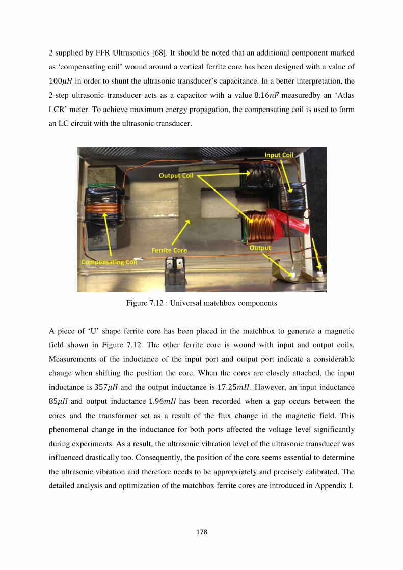
178
2 supplied by FFR Ultrasonics [68]. It should be noted that an additional component marked
as ‘compensating coil’ wound around a vertical ferrite core has been designed with a value of
100�� in order to shunt the ultrasonic transducer’s capacitance. In a better interpretation, the
2-step ultrasonic transducer acts as a capacitor with a value 8.16�� measuredby an ‘Atlas
LCR’ meter. To achieve maximum energy propagation, the compensating coil is used to form
an LC circuit with the ultrasonic transducer.
Figure 7.12 : Universal matchbox components
A piece of ‘U’ shape ferrite core has been placed in the matchbox to generate a magnetic
field shown in Figure 7.12. The other ferrite core is wound with input and output coils.
Measurements of the inductance of the input port and output port indicate a considerable
change when shifting the position the core. When the cores are closely attached, the input
inductance is 357�� and the output inductance is 17.25��. However, an input inductance
85�� and output inductance 1.96�� has been recorded when a gap occurs between the
cores and the transformer set as a result of the flux change in the magnetic field. This
phenomenal change in the inductance for both ports affected the voltage level significantly
during experiments. As a result, the ultrasonic vibration level of the ultrasonic transducer was
influenced drastically too. Consequently, the position of the core seems essential to determine
the ultrasonic vibration and therefore needs to be appropriately and precisely calibrated. The
detailed analysis and optimization of the matchbox ferrite cores are introduced in Appendix I.

179
• Phase Shifter
The phase shifter is designed to provide a full circle (360°) phase shift within the resonant
frequency range 15���~25��� of the ultrasonic transducer using both manual and remote
control [16]. As can be seen in Figure 7.13, the knob can be adjusted in order to bring the
ultrasonic vibrating system to the resonance. There is a switch that allows the gain settings to
be either 1 or 10 to inject more power into the universal matchbox (transformer). As observed
during experiments, however, a gain setting 10 will normally cause output signal
overloading. The gain of the phase shifter is frequency dependent, therefore the phase shifter
has been put before the voltage-controlled amplifier (shown in Figure 7.2 and Figure 7.3) to
limit the signal level [16]. At the back face of the phase shifter, another port is available to
perform the automatic phase shift controlled by a DC signal. In this project, however, the
phase shifter is operated manually. In other words, once the knob is adjusted to bring the
ultrasonic vibrating system to a desired resonant regime, it remains unchanged during
machining.
Figure 7.13 : Phase shifter
As explained before that the phase-amplitude characteristic of the ultrasonic vibrating system
presents a bell shape which implies little effect imposed on the phase controlled ultrasonic
vibrating system even though the resonant frequency will be shifted when the machining
condition changes. An essential drop of the ultrasonic vibration level due to the harsh
machining process can be tackled by an amplitude controller in combination with a voltage-
controlled amplifier. Observations on the frequency shift of the ultrasonic transducers when
the vibro-impact happens during experiments show a less than 0.2��� value. This slight
resonant frequency shift indicates little change in the phase-amplitude characteristics.

180
• Amplitude Controller
An amplitude controller is employed to generate a DC control voltage signal for the voltage-
controlled amplifier. Compared with the phase shifter, the amplitude controller plays a role in
supplying more power against the change in the ‘signal to be controlled’ measured by a
performance sensor. The amplitude controller circuits are shown in Figure 7.14. ‘Signal to be
controlled’ can be the 2nd
step ultrasonic vibration �2 , the current � or the power �. The
detailed working principle of the amplitude controller circuit is described below.
Figure 7.14 : Amplitude controller
Figure 7.15 illustrates the amplitude controller circuits’ components. In the beginning, the
True RMS-to-DC converter (AD536ADJ details in [72]) collects the performance sensors’
samples marked as ‘�������’ which is the 2nd
step ultrasonic vibration, the current or the
instantaneous power depending on the feedback type. After this, a 12�Ω resistor is placed in
case of signal overload. The true RMS value of the sensor signal is further compared with a
DC voltage determined by a potential meter 50�Ω which is placed between a 12� power
supply and the earth potential. During operation, the potential meter 50�Ω is adjusted to
ensure a similar signal level between the negative terminal and the positive terminal. The
difference is further amplified by an OP07 (details in [73]) offset amplifier. A 50�Ω
potential meter has been connected in the negative feedback loop of the OP07 amplifier
which is adjustable to determine the negative feedback loop gain. Subsequently, a DC voltage
is generated marked as ‘���’. Theoretically, during vibro-impact process the sensor signal

181
will drop due to energy loss on the tip of a drill bit. This drop will give rise to a decrease at
the positive terminal of the offset amplifier OP07. Hence, a negative difference value will be
produced which is amplified by the adjustable potential meter 50�Ω in order to bring the ′���′ to the operational zone for the voltage-controlled amplifier further on (the voltage-
controlled amplifier will be introduced next).
Figure 7.15 : Amplitude controller circuits diagram
• Voltage-Controlled Amplifier
In order to implement the negative feedback loop, a voltage-controlled amplifier (VCA810
details in [74]) has been placed after the phase shifter. The structure of the voltage-controlled
amplifier circuit is shown in Figure 7.16 and the detailed connection of the components is
illustrated in Figure 7.17.
As can be seen, the input to the voltage-controlled amplifier is an AC actuating signal which
is the output of the phase shifter. Depending on the feedback type, the actuating signal could
be the 2nd
step ultrasonic vibration measured by the inductive sensor during mechanical
feedback control, the current flowing through the piezoelectric transducer measured by the
current sensor during current feedback control and during power feedback control. A 10�Ω
potential meter (normally not used or tuned to be 0�Ω) has been put after the actuating signal
in case of signal overloading. The control input to the voltage-controlled amplifier is the DC
voltage signal generated by the amplitude controller marked as ‘���’.

182
Figure 7.16 : Voltage-controlled amplifier
Figure 7.17 : Voltage-controlled amplifier circuit diagram
The main improvement of the autoresonant control on Ultrasonically Assisted Drilling
(UAD) in comparison with the previous autoresonant control on Ultrasonically Assisted
Turning (UAT) is the replacement of the limiter with a DC-coupled, wideband, continuously
variable, voltage-controlled gain amplifier VCA810. The application of the VCA810 not only
gets rid of the use of either a low-pass filter or a Butterworth filter to recreate a sine wave
supplied voltage signal base on a square wave produced by the limiter, but also reduces the
strong nonlinearity caused by the limiter. Basically, the operational range of the VCA810 is
between −40��~40�� with a control voltage varying from 0� to −2� (���). Within this

183
range, VCA810 is able to attenuate or amplify a sine wave without breaching its original
waveform.
Being different from the autoresonant control principle described in section 5.1 (numerical
simulations), the experiments employ the phase shifter, the amplitude controller and the
voltage-controlled amplifier simultaneously and process them in real time. It should be re-
emphasized that the phase shifter is an essential element in positive feedback loop for
autoresonant control and the amplitude controller acts in the negative feedback loop which is
an element for additional power injection during harsh machining conditions.
7.2.2 Data Recording Units (Box 3)
There are 3 components used to record and process the data of the autoresonant controlled
ultrasonic vibrating system which are the True RMS-to-DC converters (AD536ADJ details in
[72]), a 4-channel PicoScope and a computer. Each of them will be introduced below.
In Figure 7.18 the True RMS-to-DC converter circuit is shown. The input to the circuit is the
AC signal to be observed. The RMS converter collects samples and calculates the DC level
RMS value which is transferred to the output port. In order to understand the detailed
connections in the circuit board, the electrical diagram is drawn and presented in Figure 7.19.
Figure 7.18 : True RMS Converter circuit

184
Figure 7.19 : True RMS Converter circuit diagram
The input ‘���’to the RMS converter is the AC signal to be observed. In this project, several
sensor signals are monitored simultaneously depending on the feedback type which might be
the inductive sensor’s output (the 2nd
step ultrasonic vibration �2 ), the ‘signal to be
controlled’ (the signal used to determine the required amount of effort for the ultrasonic
vibrating system) and the voltage-controlled amplifier’s output (the universal amplifier’s
input, actual original driving signal of the ultrasonic transducer) as shown in Figure 7.2 and
Figure 7.3. A 1�� capacitor has been put after the input AC signals to smooth them and
eliminate the DC components. In order to filter the unwanted high frequency noises, 2 RC
circuits (resistance 10�٠and capacitance 1��) [76] have been employed before the pure DC
RMS signal ‘����’ is recorded. It should be noted that a same set of RC filters are connected
to earth potential. The reason for this is the rotational motion of the ultrasonic transducer and
the high power voltage inverter used to drive the lathe had a great impact on the signal
recording during experiments. Such effect results in a non-zero value in the earth potential.
This is likely caused by the high frequency components and therefore low pass filters are
used to ensure a zero signal level in the earth potential. There are 4 sets of RMS converters
available in the experiments.
In order to record the RMS signals produced by the True RMS-to-DC converters, a 4-channel
PicoScope (PicoScope 4424 with a bandwidth 20��� , details in [82]) was used. The
PicoScope is connected to a TOSHIBA laptop to process the RMS signals for further

185
analysis. The PicoScope allows maximum 4 signals to be monitored and recorded
simultaneously during experiments.
7.3 Autoresonant Control Analysis for Different Strategies and
Drill Bits
In this section, fixed frequency control, mechanical feedback, current feedback and power
feedback on 2 sizes of drill bits with a fixed rotational speed of the spindle in combination
with several feed rates are examined. The listed control strategies are applied on 2 sizes of
drill bits which are 3mm and 6mm in diameter. As explained in [15], only in drilling small
holes with diameters smaller than 3mm a drill bit can be treated as a small lamp mass
attached to the ultrasonic transducer. In contrast, with an increase in diameters of holes a
successful application of the Ultrasonically Assisted Drilling (UAD) needs acoustical
matching of the drill bit as a continuous system with a transducer. Therefore, a drill bit
greater than 3mm in diameter with a reasonable length, complicated geometry and dynamics
should be treated as an additional step of waveguide (concentrator).
Figure 7.20 : Properly adjusted ultrasonic vibrating system waveform
Figure 7.20 illustrates an ideal situation of a possible waveform of a properly tuned 2-step
ultrasonic transducer with a drill bit during resonance. It has been experimentally proved that
at the end of 2nd
step concentrator the ultrasonic vibration achieves a maximal without a drill
bit attached. However, a drill bit attachment requires a proper acoustic matching with the
ultrasonic transducer in order to ensure the additional step (drill bit) as a continuation of the
original vibrating system. Due to the material and geometry difference, such waveform

186
shown in Figure 7.20 is difficult to be achieved which has been confirmed experimentally.
On the other hand, however, the 2nd
step ultrasonic vibration is physically in relation with the
ultrasonic vibration magnitude on the tip of a drill bit. Therefore, owing to the unavailable
information of the ultrasonic vibration on the tip of a drill bit during machining, the ultrasonic
vibration at the end of the 2nd
step concentrator �2 has been selected as the observation point
for the ultrasonic vibration.
7.3.1 A 3mm Diameter Standard Drill Bit
During the Ultrasonically Assisted Drilling (UAD) process, a 3mm diameter HSS-Co 8% tin
coated heavy duty jobber drill bit was used. Point angle of the 3mm drill bit is 135° and helix
angle is 28°. The overall length is 61mm and flute length is 33mm with weight 28 grams. 4
grub screws were used to clamp a 3mm drill bit at the end of the 2nd
step concentrator �2
uniformly and tightly from 4 directions. The entire ultrasonic vibrating system was properly
centred with the help of a centring gauge. Such a 3mm drill bit needs no proper tuning since
it can be treated as a small mass. The rotational speed of the spindle for the application of the
3mm drill bit was fixed as 40rev/min. 3 feed rates 0.03mm/rev, 0.06mm/rev and 0.09mm/rev
were applied. Experimental setup of a 3mm drill bit application during the autoresonant
control is shown in Figure 1.1.
7.3.1.1 Frequency Control
In frequency control, a SFG-2110 synthesized function generator was used to generate an
actuating sinusoidal signal with a resonant frequency and proper amplitude which is supplied
to the universal amplifier and the universal matchbox (transformer) to drive the ultrasonic
vibrating system. During the Ultrasonically Assisted Drilling (UAD), RMS of the 2nd
step
ultrasonic vibration �2 was measured by an inductive sensor because the information of the
ultrasonic vibration is unavailable on the tip of a 3mm drill bit. Meanwhile, the RMS of the
control effort which is the actual original driving signal of the universal amplifier is recorded.
As introduced before that the linear operational interval of universal amplifier is ±70� with a
gain 65 which corresponds to a RMS 0.76� , any amplitude greater than this will be
truncated. However, certain reasonable overloading is necessary for high feed rate. Results of
the frequency control are illustrated in Figure 7.21.
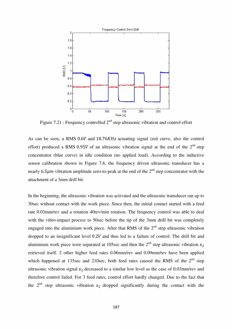
187
Figure 7.21 : Frequency controlled 2nd
step ultrasonic vibration and control effort
As can be seen, a RMS 0.6� and 18.76��� actuating signal (red curve, also the control
effort) produced a RMS 0.95� of an ultrasonic vibration signal at the end of the 2nd
step
concentrator (blue curve) in idle condition (no applied load). According to the inductive
sensor calibration shown in Figure 7.6, the frequency driven ultrasonic transducer has a
nearly 6.5�� vibration amplitude zero-to-peak at the end of the 2nd
step concentrator with the
attachment of a 3mm drill bit.
In the beginning, the ultrasonic vibration was activated and the ultrasonic transducer ran up to
30sec without contact with the work piece. Since then, the initial contact started with a feed
rate 0.03mm/rev and a rotation 40rev/min rotation. The frequency control was able to deal
with the vibro-impact process to 50sec before the tip of the 3mm drill bit was completely
engaged into the aluminium work piece. After that RMS of the 2nd
step ultrasonic vibration
dropped to an insignificant level 0.2� and thus led to a failure of control. The drill bit and
aluminium work piece were separated at 105sec and then the 2nd
step ultrasonic vibration �2
retrieved itself. 2 other higher feed rates 0.06mm/rev and 0.09mm/rev have been applied
which happened at 135sec and 210sec, both feed rates caused the RMS of the 2nd
step
ultrasonic vibration signal �2 decreased to a similar low level as the case of 0.03mm/rev and
therefore control failed. For 3 feed rates, control effort hardly changed. Due to the fact that
the 2nd
step ultrasonic vibration �2 dropped significantly during the contact with the

188
aluminium work piece, the ultrasonic vibrating system lost its benefits hence no obvious feed
force reduction was observed.
Figure 7.22 : Frequency control in association with amplitude control 2nd
step ultrasonic
vibration and control effort
In order to explore whether the 2nd
step ultrasonic vibration can be maintained with the help
of the amplitude control system, negative feedback loop shown in Figure 7.2 and Figure 7.3
has been connected to the frequency controlled ultrasonic vibrating system. During this
process, the function generator’s output signal with a pre-defined frequency acts as the
‘actuating signal’ and the inductive sensor’s output (the RMS of the 2nd
step ultrasonic
vibration) is the ‘signal to be controlled’. The phase shifter was removed from the loop and
the output of the voltage-controlled amplifier is supplied to the universal amplifier to drive
the ultrasonic vibrating system. Results are shown in Figure 7.22.
As can be seen in Figure 7.22, the initial contact between the 3mm drill bit and the work
piece took place at 40sec with a rotation 40rev/min and a feed rate 0.03mm/rev. RMS of the
2nd
step ultrasonic vibration �2 dropped moderately and the RMS of the control effort
increased against the drop in the 2nd
step ultrasonic vibration �2. This process implies a fast
and accurate working principle of the negative feedback control loop which is to compensate
the decrease in the RMS of the 2nd
step ultrasonic vibration signal. The drill bit and the work
piece were separated at 175sec. Feed rates 0.06mm/rev and 0.09mm/rev were applied at

189
210sec and 315sec. As a result, RMS of the 2nd
step ultrasonic vibration decreased to 0.4�
and RMS of the control effort increased considerably to 1.5� for both feed rates which
completely exceeded the linear operational region of the universal amplifier. Drilling depths
for three feed rates were 2.7mm, 2.8mm and 3.6mm.
In comparison with the frequency control, the ultrasonic vibrating system with the help of the
amplitude control system was able to deal with a low feed rate 0.03mm/rev. However, for
high feed rates 0.06mm/rev and 0.09mm/rev, the 2nd
step ultrasonic vibration �2 decreased
considerably even if the amplitude control system generated enormous voltage for the
ultrasonic transducer to compensate for the change in the sensor signal. The remarkable drop
in the inductive sensor’s signal for high feed rate can be attributed to the high Q factor of the
ultrasonic vibrating system attached with a 3mm drill bit. A high feed rate driven ultrasonic
vibrating system had a larger resonant frequency shift in the frequency-amplitude
characteristic which consequently caused the ultrasonic vibration magnitude �2 decreased to
a low level. Nonetheless, the stable RMS of the 2nd
step ultrasonic vibration with the help of
amplitude control system for 0.06mm/rev and 0.09mm/rev feed rates showed a 0.4� value as
a result of tremendously increased voltage supply. However, since the RMS of the control
efforts completely exceeded the linear operational zone of the universal amplifier for high
feed rates, RMS of the 2nd
step ultrasonic vibration would not increase over 0.4�. In contrast,
as shown in Figure 7.21, high feed rates resulted in a 0.2� stable RMS of the 2nd
step
ultrasonic vibration without the amplitude control participation.
In order to verify the existence of the ultrasonic vibration on the tip of the 3mm drill bit
during drilling, feed force measurement has been recorded by the Kistler dynamometer.
Results are shown in Figure 7.23. The initial contact between the 3mm drill bit and the work
piece happened at 30sec. Due to the participation of the amplitude control, Ultrasonically
Assisted Drilling (UAD) lasted for 65secs with a spindle rotation 40 rev/min and a feed rate
0.03mm/rev. Thrust force during this process is less than 5�. At 95sec, both the frequency
generator and the control system were switched off and the ultrasonic vibration disappeared.
The steady feed force turned into nearly 25� as a result of the Conventional Drilling (CD)
domination. The control system was turned on after the separation of the drill bit and the
work piece and higher feed rates 0.06mm/rev and 0.09mm/rev were applied at 185sec and
340sec. After the Kistler dynamometer’s output signal became stable, the control system was
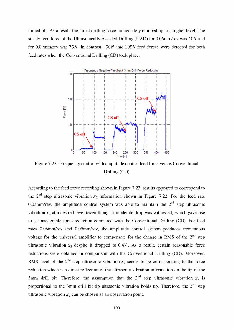
190
turned off. As a result, the thrust drilling force immediately climbed up to a higher level. The
steady feed force of the Ultrasonically Assisted Drilling (UAD) for 0.06mm/rev was 40� and
for 0.09mm/rev was 75�. In contrast, 50� amd 105� feed forces were detected for both
feed rates when the Conventional Drilling (CD) took place.
Figure 7.23 : Frequency control with amplitude control feed force versus Conventional
Drilling (CD)
According to the feed force recording shown in Figure 7.23, results appeared to correspond to
the 2nd
step ultrasonic vibration �2 information shown in Figure 7.22. For the feed rate
0.03mm/rev, the amplitude control system was able to maintain the 2nd
step ultrasonic
vibration �2 at a desired level (even though a moderate drop was witnessed) which gave rise
to a considerable force reduction compared with the Conventional Drilling (CD). For feed
rates 0.06mm/rev and 0.09mm/rev, the amplitude control system produces tremendous
voltage for the universal amplifier to compensate for the change in RMS of the 2nd
step
ultrasonic vibration �2 despite it dropped to 0.4� . As a result, certain reasonable force
reductions were obtained in comparison with the Conventional Drilling (CD). Moreover,
RMS level of the 2nd
step ultrasonic vibration �2 seems to be corresponding to the force
reduction which is a direct reflection of the ultrasonic vibration information on the tip of the
3mm drill bit. Therefore, the assumption that the 2nd
step ultrasonic vibration �2 is
proportional to the 3mm drill bit tip ultrasonic vibration holds up. Therefore, the 2nd
step
ultrasonic vibration �2 can be chosen as an observation point.

191
7.3.1.2 Mechanical Feedback
Mechanical feedback employs the actual ultrasonic vibration of the 2nd
step �2 measured by
an inductive sensor as both the ‘actuating signal’ and the ‘signal to be controlled’ as indicated
in Figure 7.2 and Figure 7.3. The aim of this strategy is to maintain the ultrasonic vibration
on the tip of the 3mm drill bit at a constant during drilling. This is done through keeping the
2nd
step ultrasonic vibration �2 stable based on the assumption that it is in proportion with the
ultrasonic vibration on the tip of the 3mm drill bit. Since the mechanical feedback measures
and controls the mechanical vibration directly, it is supposed to have the overall best results.
The operational procedure of mechanical feedback control is that the phase shifter was
manually adjusted in order to bring the RMS of the 2nd
step ultrasonic vibration �2 to the
resonance. After this the potential meter ‘50�Ω’ shown in Figure 7.15 connected between the
negative port of offset amplifier OP07 and output ‘���’ was tuned to the maximum in order
to allow the negative feedback to have the maximum gain. Then the potential meter marked
as ‘50�Ω’ connected between the 12� and the earth was tuned until both the outputs of the
voltage-controlled amplifier (control effort) and the inductive sensor’s output presented a
reasonable peak value. During drilling, the phase shifter and each element in the negative
feedback were fixed. Results of the mechanical feedback are shown in Figure 7.24.
Figure 7.24 : Mechanical feedback controlled 2nd
step ultrasonic vibration and control effort
The red curve represents the RMS of the control effort and the blue line is the RMS of the 2nd
step ultrasonic vibration �2. An ultrasonic vibration level 0.85� was obtained with a RMS of

192
the control effort 0.3�. As can be seen, the initial contact between the drill bit and the work
piece happened at 30sec with a 0.03mm/rev feed rate and a 40rev/min rotation. As the drill
bit was engaged deeper into the material, the ultrasonic vibrating system required more power
to deal with the energy loss on the 3mm drill bit tip. RMS of the control effort increased from
0.3� to more than 0.4� . Meanwhile, RMS of the 2nd
step ultrasonic vibration �2 was
maintained at a constant level. At 170sec, the drill bit and the work piece were separated with
a recovery of both RMS in the 2nd
step ultrasonic vibration �2 and RMS in the control effort.
At 205sec, a higher feed rate 0.06mm/rev was applied. The Ultrasonically Assisted Drilling
(UAD) process lasted for 120secs with the control effort increased from 0.3� to more than
0.5� which is twice as high as of the previous feed rate. RMS of the 2nd
step ultrasonic
vibration slightly decreased as the drill bit penetrated deeper into the work piece but still can
be kept at a desired level. The drill bit was removed from the work piece at 325sec.
0.09mm/rev feed rate was applied at 360sec. For this feed rate, the 2nd
step ultrasonic
vibration �2 could still be maintained even if a more obvious drop was witnessed when the
drill bit was deeply engaged. RMS of the control effort increased from 0.3� to nearly 0.7�.
For all 3 feed rates, the control effort climbed up gradually against the change in the
inductive sensor signals and as the feed rate increased, the control effort showed a
proportional trend as the change in the RMS of the 2nd
step ultrasonic vibration �2 which
seemed to drop proportionally. It should be emphasized that the resonant frequency has been
monitored; the maximal change in the resonant frequency was no more than 0.2��� which
hardly altered the phase in the phase-amplitude characteristic of the ultrasonic vibrating
system. Drilling depths for three feed rates were 2.8mm, 4.8mm and 7.8mm.
In order to examine the existence of the ultrasonic vibration on the tip of the 3mm drill bit,
feed force was monitored during drilling and results are shown in Figure 7.25. The initial
contact with a 0.03mm/rev feed rate and a 40rev/min rotation happened at 15sec with the
mechanical feedback control and the Ultrasonically Assisted Drilling (UAD) process lasted
for 65secs until the feed force stabilised. The thrust force level during this period was low. At
80sec, the mechanical feedback control system was switched off which resulted in a sudden
increase in the thrust force to 25� . This process showed the transition from the
Ultrasonically Assisted Drilling (UAD) to the Conventional Drilling (CD). The drill bit and
the work piece were separated at 135sec and the control system was turned on. A higher feed
rate 0.06mm/rev was applied at 170sec and feed force increased to 6�. This Ultrasonically

193
Assisted Drilling (UAD) process lasted until 225sec with a switch-off of the mechanical
feedback control system. As a result, Conventional Drilling (CD) took place which produced
a nearly 60� force. Feed rate 0.09mm/rev was executed at 330sec with a sudden increase in
the feed force which confirmed the drill bit tip penetration process into the material. The
thrust force gradually arrived at its stable regime with an approximately 12� value. The
mechanical feedback system was turned off at 400sec which resulted in a considerable
increase in the thrust force to more than 110�. Such tremendous force reductions from the
Conventional Drilling (CD) to the Ultrasonically Assisted Drilling (UAD) for 3 feed rates
proved a strong ultrasonic vibration at the tip of the 3mm drill bit. In contrast to the frequency
control with help of the amplitude control shown in Figure 7.22 and Figure 7.23, mechanical
feedback control was able to handle a feed rate up to 0.09mm/rev.
Figure 7.25 : Mechanical feedback feed force reduction versus Conventional Drilling (CD)
7.3.1.3 Current Feedback
Current feedback uses a current probe which is placed between the universal matchbox
(transformer) and the ultrasonic transducer to measure the current � flowing through the
piezoelectric transducer and consider it as both the ‘actuating signal’ and the ‘signal to be
controlled’ in the feedback loop. This strategy aims at maintaining the 2nd
step ultrasonic
vibration �2 that is proportional to the ultrasonic vibration on the tip of the 3mm drill bit at a
constant level during drilling. This is done through stabilising the current signal �. Since
current feedback controls the 2nd
step ultrasonic vibration �2 in an indirect way, the

194
effectiveness of the control entirely relies on the dynamic coupling between the current � and
the mechanical vibration �2 characteristics. The experimental procedure is the phase shifter
was adjusted to reach the current resonance and then the potential meter shown in Figure 7.15
marked as ‘50�Ω’ was tuned to the maximum to allow the maximum gain in the negative
feedback loop and the other ‘50�Ω’ potential meter was adjusted until both the output of the
voltage-controlled amplifier (control effort) and the output of the current probe reached
resonance. It should be addressed that no band-pass filters or Butterworth filters were
employed to tackle the ambiguity characteristic of the current signal during drilling.
However, a Butterworth filter is indispensable during the numerical simulation for the
electrical feedback. This controversy questions the accuracy and applicability of the current
calculation equation (4.62) in practice. Again, the piezoelectric effect is a very complicated
process. Therefore, the current signal in reality might include other variables besides only the
actuation force �0 and the supplied voltage �. Each element in the current feedback control
system remained unchanged during drilling. Results of the current feedback are presented in
Figure 7.26.
Figure 7.26 : Current feedback controlled 2nd
step ultrasonic vibration, current and control
effort
Figure 7.26 represents the oscilloscope readings of the drilling experiment with current
feedback control system. Blue curve is the RMS of the 2nd
step ultrasonic vibration �2, pink
curve stands for the RMS of the current � and red curve represents the RMS of the control

195
effort. A RMS of the 2nd
step ultrasonic vibration �2 value 0.85� was obtained with a RMS
value of 0.33� for the control effort and a RMS value of 0.65� for the current �. Same as the
mechanical feedback experiment, 3 different feed rates have been applied which were:
0.03mm/rev (at 15sec), 0.06mm/rev (at 185sec) and 0.09mm/rev (at 345sec). For all the 3
intervals when the feed was applied, the increase in the control effort was observed which
seemed to rise proportionally. This increase in the control effort demonstrated the control
system was working to compensate for the changes in the current sensor’s output which was
caused by the applied load. The current sensor’s output, on the other hand, slightly dropped
during drilling but could still be maintained at a desired level. This showed the efficiency of
the control system as it was able to stabilise the amplitude of the ‘signal to be controlled’, in
this case, current � . In terms of the inductive sensor’s output, it demonstrated moderate
decreases for 3 feed rates which implied a strong dynamic coupling between the current � and
the mechanical vibration �2 characteristic in reality. In a better interpretation, stabilising the
ultrasonic vibration �2 through keeping the current � was an effective method. Consequently,
the reliability and convenience of the current feedback control was confirmed. The resonant
frequency shift during the Ultrasonically Assisted Drilling (UAD) process was no more than
0.2��� which indicated little phase change in the amplitude-phase characteristic of the
current signal. Drilling depths for three feed rates were 3.0mm, 5.2mm and 7.5mm.
Figure 7.27 : Current feedback feed force reduction versus Conventional Drilling (CD)

196
The feed force reduction experiment from the Conventional Drilling (CD) to the current
feedback controlled Ultrasonically Assisted Drilling (UAD) has been executed. Results are
shown in Figure 7.27. 3 feed rates were executed with the autoresonant controlled ultrasonic
vibration which happened at 25sec, 160sec and 330sec. When the Ultrasonic Assisted
Drilling (UAD) process stabilised, the current feedback control system was turned off and
these occurred at 80sec, 240sec and 400sec. As a result, the steady average feed force rose
significantly to a higher level. Therefore, considerable feed force reduction from the
Ultrasonically Assisted Drilling (UAD) to the Conventional Drilling (CD) for 3 feed rates
indicated a strong ultrasonic vibration at the tip of the 3mm drill bit. Current feedback control
worked efficiently to maintain the ultrasonic vibration on the tip of the 3mm drill bit during
vibro-impact through stabilising the current signal and hence is a reliable autoresonant
control strategy.
7.3.1.4 Power Feedback
Figure 7.28 : Power feedback controlled 2nd
step ultrasonic vibration, power and control
effort
Power feedback employs a power sensor shown in Figure 7.7 (manufactured in the ultrasonic
machining laboratory, Loughborough University) to measure the scaled instantaneous power
and applies it as the ‘signal to be controlled’ in the negative feedback loop. Current flows
through the piezoelectric transducer acts as the ‘actuating signal’ to form the positive
feedback. This strategy aims at maintaining the 2nd
step ultrasonic vibration �2 which is in

197
proportion to the ultrasonic vibration on the tip of the 3mm drill bit at a constant level
through stabilising power during drilling. The experimental procedure is the phase shifter and
potential meter marked as 100�Ω as well as 50�Ω in Figure 7.7 were properly adjusted. The
50�Ω potential meter in Figure 7.15 was tuned to the maximum to achieve the maximum
gain and the other 50�Ω potential meter was adjusted to reach power signal resonance which
was designed to have a similar level of current RMS in the current feedback. Each element in
the power feedback control remained fixed during drilling. Results of the power feedback are
showed in Figure 7.28.
Blue curve represents the RMS of the 2nd
step ultrasonic vibration �2 measured by the
inductive sensor, pink curve stands for RMS of the scaled instantaneous power measured by
the power sensor and red curve is RMS the of control effort which is the output of the
voltage-controlled amplifier. A RMS 0.95� of the 2nd
step ultrasonic vibration �2, a RMS
0.45� of the control effort and a RMS 0.78� of the instantaneous power were obtained
initially. In this instance, 3 feed rates 0.03mm/rev, 0.06mm/rev and 0.09mm/rev were applied
which took place at 35sec, 200sec and 340sec. The control effort can be clearly observed as it
showed some difference from the mechanical feedback and the current feedback. RMS of the
power sensor’s output indicated a roughly constant level for low feed rate 0.03mm/rev which
required a little increase in the control effort. In comparison, RMS of the power for high feed
rates presented obvious drops which gave rise to the enormous increase in the control effort.
In addition, high feed rates caused the control effort completely exceeded the linear
operational range of the universal amplifier. Therefore the resultant supplied voltage would
be partially truncated. This was not observed during mechanical feedback and current
feedback whose control efforts were strictly within the linear zone.
In terms of the inductive sensor’s output, there was a slightly more decrease for 3 feed rates
than the other 2 feedbacks even though the control effort was tremendous. This implies a
weakened dynamic coupling between the mechanical vibration characteristic and the
instantaneous power signal than the current for the loaded ultrasonic vibrating system.
Resonant frequency shift monitored during the power feedback controlled Ultrasonically
Assisted Drilling (UAD) was no more than 0.2��� which meant little change in the
amplitude-phase characteristics of the power signal. Drilling depths for three feed rates were
2.9mm, 4.8mm and 7.8mm.

198
Feed force reductions from the power feedback controlled Ultrasonically Assisted Drilling
(UAD) to the Conventional Drilling (CD) is illustrated in Figure 7.29. 3 feed rates
0.03mm/rev, 0.06mm/rev and 0.09mm/rev were examined which happened at 20sec, 220sec
and 395sec. Power feedback controlled ultrasonic vibrating system was switched on initially
and after certain depth of the Ultrasonically Assisted Drilling (UAD) with a stabilization of
the Kistler dynamometer’s output, control was turned off. As can be observed, tremendous
feed force reduction indicated strong ultrasonic vibrations on the tip of the 3mm drill bit
during vibro-impact for three feed rates. The ultrasonic vibration amplitude can be
maintained through keeping the power at a constant level. Similar to the current feedback,
this remote control strategy also emphasises the convenience and feasibility of the
employment of the instantaneous power as a feedback signal.
Figure 7.29 : Power feedback feed force reduction versus conventional drilling
7.3.1.5 Summary
In the above sections, the listed control strategies have been explored on a 2-step ultrasonic
transducer attached with a 3mm drill bit shown in Figure 1.1. In order to analyse the results
more thoroughly, the maximum deflection in the RMS of the 2nd
step ultrasonic vibration �2
from the desired levels, feed force reductions from the Ultrasonically Assisted Drilling
(UAD) to the Conventional Drilling (CD) for each feed rate have been shown in Table 7.2
and Table 7.3.

199
As can be seen in Table 7.2, the frequency control seems lacking of ability to maintain the 2nd
step ultrasonic vibration �2 with a constant control effort as the maximal deviations from the
desired levels present considerably large values. Therefore, no feed force reductions have
been observed for 3 feed rates. With the help of the amplitude control system, the RMS of the
2nd
step ultrasonic vibration �2 with a low feed rate 0.03mm/rev can be maintained at a
desired level with 7.5% deflection. Feed force reduction for the 0.03mm/rev feed rate is
phenomenal which presents an 88.9% value shown in Table 7.3. For the high feed rates
0.06mm/rev and 0.09mm/rev, the amplitude control system generated huge control efforts
against the considerable drops in the inductive sensor’s output. However, the improvement in
the RMS of the 2nd
step ultrasonic vibration �2 is small compared with frequency control.
This is due to the high Q factor of the ultrasonic vibrating system where the resonant
frequency shifted under significant applied load which resulted in a considerable amplitude
drop in the frequency-amplitude characteristic. Moreover, even though huge control effort
was produced by the negative feedback loop to the universal amplifier, no further benefit
could be achieved from the increased control effort because it completely exceeded the linear
zone. Reasonable feed force reductions 24% and 25.5% have been witnessed for high feed
rates shown in Table 7.3. This can be ascribed to the huge control effort.
Table 7.2 : Maximum deflection in RMS of the 2nd
step ultrasonic vibration of a 3mm drill bit
application
Strategy
Deflection
Frequency
Control
Freq+Amp
control
Mechanical
Feedback
Current
Feedback
Power
Feedback
0.03mm/rev
78.7%
7.5%
0.5%
1.2%
2.5%
0.06mm/rev
79.8%
56.9%
1.2%
2.4%
6.3%
0.09mm/rev
80.8%
58.1%
3.4%
3.7%
6.7%
For the 3 autoresonant control strategies, they are able to keep the nonlinear resonant mode of
the oscillations in ill-defined and time changing conditions. A completed investigation on a
3mm drill bit application reveals that mechanical feedback shows an overall best performance

200
with a minimum deflection in RMS of the 2nd
step ultrasonic vibration �2 from the desired
levels shown in Table 7.2 and the largest force reductions shown in Table 7.3 for 3 feed rates.
This superior control can be ascribed to the fact that mechanical feedback employs the 2nd
step ultrasonic vibration information �2 as the ‘signal to be controlled’ and manipulates it
directly as the location of the sensor reflects the true ultrasonic vibration information. In
contrast, current feedback shows a slightly worse control in terms of the RMS of the 2nd
step
ultrasonic vibration �2 deflection and feed force reduction for 3 feed rates. To this point, it
can be concluded that the characteristic of the current � is physically and strongly coupled to
the mechanical vibration �2 . Therefore, such indirect control strategy realises the remote
control possibility for industrial use. Power feedback presents an overall worst performance
compared with the other 2 strategies in the sense of maximal deviation in the RMS of the 2nd
step ultrasonic vibration �2 from the desired levels. This control strategy is debatable,
because as the vibro-impact process continues, a drill bit penetrates deeper into the work
piece and therefore larger power consumption from the piezoelectric transducer is required.
However, the power feedback control is to maintain the RMS of the ultrasonic vibration �2
through keeping the power at a constant level rather than increasing it. It is strongly
recommended that the overall power should be increased in the power feedback control in
order to stabilise the ultrasonic vibration level. In contrast, in current feedback, current signal
is to be maintained at a desired level and this is done through increasing the supplied voltage
(control effort) to the piezoelectric transducer. As a result, the overall power during the vibro-
impact for the current feedback will be higher than a prescribed level.
Table 7.3 : Feed force reduction of a 3mm drill bit application
Strategy
Reduction
Freq+Amp
control
Mechanical
Feedback
Current
Feedback
Power
Feedback
0.03mm/rev
88.9%
90.2%
89.2%
96.2%
0.06mm/rev
24.0%
89.8%
88.4%
89.1%
0.09mm/rev
25.5%
88.4%
87.8%
84.4%

201
However, in terms of the feed force reduction, power feedback has a comparable level with
the current feedback. For the low feed rate the feed force reduction is even superior over
mechanical feedback. This is due to the higher level of control effort that the power feedback
generated which can be seen in Figure 7.28. It should be mentioned that the control effort
level entirely depends on the change in the ‘signal to be controlled’ (feedback sensor’s
output). Even though drops were more obvious in the RMS of the 2nd
step ultrasonic vibration
for 3 feed rates for the power feedback, considerable feed force reduction results prove it is
still an efficient and valid control strategy. It should be re-emphasized that electrical feedback
strategies need neither band-pass filters nor Butterworth filters which again highlights the
difference between the piezoelectric transducer in theory and piezoelectric effect in practice.
Generally speaking, by observing the results shown in Table 7.2 and Table 7.3, improvement
of using the autoresonant control from the frequency control even with the help of the
amplitude control system is remarkable, especially in dealing with high Q factor oscillation
systems. In order to explore which control strategy presents the overall best control, surface
roughness examination will be presented later which is a direct informative reflection of the
control.
7.3.2 A 6mm Diameter Standard Drill Bit
The 6mm drill bit used during Ultrasonically Assisted Drilling (UAD) experiments is a HSS-
Co 8% tin coated heavy duty jobber drill bit. Point angle of such a 6mm drill bit is 135° and
helix angle is 28°. The overall length is 93mm and the flute length is 57mm, it weighs 154
grams. The autoresonant control strategies and the frequency control were applied to the 2-
step ultrasonic transducer shown in Figure 1.1 attached with a 6mm drill bit. Unfortunately,
the 2-step ultrasonic transducer was not powerful to drive the 6mm drill bit during drilling.
Therefore, a more powerful ultrasonic transducer is strongly recommended. A 4-
piezoceramic rings transducer was available in the ultrasonic machining laboratory in
Wolfson School of Mechanical and Manufacturing Engineering in Loughborough University
and it was employed for the investigation of the autoresonant control on a 6mm drill bit
application. The 4-piezoceramic rings powerful transducer structure and dimensions are
shown in Figure 7.30.

202
Figure 7.30 : 4-piezoceramic rings ultrasonic transducer: (a) structure, (b) dimensions
As can be seen, there are 2 pairs of piezoceramic rings connected together. The back section
of the concentrator is made from steel and the concentrator material is titanium. The
ultrasonic transducer was assembled with a tensioning bolt. In order to fix a 6mm drill bit to
the ultrasonic transducer, a 2-step aluminium adaptor has been manufactured which was
screwed to the titanium concentrator. At the end of the aluminium adaptor, 4 grub screws
were used to hold a 6mm drill bit. As introduced in Figure 7.20, an application of a 6mm drill

203
bit to the ultrasonic transducer needs acoustical matching as such a diameter size should be
treated as an additional step of the waveguide (concentrator).
7.3.2.1 A 6mm Drill Bit Proper Tuning
Figure 7.31 : A 6mm drill bit proper tuning
Theoretically, the waveform shown in Figure 7.20 for an appropriately adjusted ultrasonic
vibrating system should be achieved. In practice, however, this is difficult to be realized due
to the material difference, geometry complexity etc. Therefore, in order to properly tune the
6mm drill bit so as to enable it to match with the ultrasonic transducer acoustically, the
following experiment has been performed. 30mm from the end of the shank of a 6mm drill
bit was selected which was then divided into 6 equal segments with a marker. The drill bit
was fixed to the ultrasonic transducer with the shank inserted to the following length: 5mm,
10mm, 15mm, 20mm, 25mm and 30mm. The resonant frequencies of different insertion
depths of the 6mm drill bit of the ultrasonic vibrating system were explored with the help of
the SFG-2110 synthesized function generator. A thin reflection film was attached to the tip of
the 6mm drill bit in order to record the ultrasonic vibration magnitude at resonance. The
insertion depth which generates the maximum vibration magnitude at the tip of the drill bit
will be used for the investigation of the autoresonant control. Results are shown in Figure
7.31. Experiment revealed that an insertion depth of 25mm of the 6mm drill bit shank into the
ultrasonic transducer was able to develop the largest vibration magnitude 11.2�� zero-to-

204
peak. Therefore, the 6mm drill bit was fixed with an insertion depth 25mm into the tool
holder.
Figure 7.32 : Q factor of the powerful ultrasonic transducer: (a) no tool, (b) a 6mm drill bit
In order to study the difficulties that might be encountered during the investigation of the
listed autoresonant control strategies, the Q factor of the 4-rings ultrasonic transducer shown
in Figure 7.30 with and without the attachment of a 6mm drill bit was experimentally
explored. Results are shown in Figure 7.32. (a) represents the frequency-amplitude
characteristics of the 4-rings ultrasonic transducer. (b) shows the frequency-amplitude
characteristics of the 4-rings ultrasonic transducer attached with a 6mm drill bit. As can be
seen, a 6mm drill bit hardly shifts the resonant frequency of the 4-ring ultrasonic transducer;
however, it considerably narrows down the half power bandwidth of the characteristic which
results in a tremendous increase in Q factor value. Experiments data suggests a Q factor value
of the 4-rings ultrasonic transducer without a 6mm drill bit attachment 20 (a). In comparison,
a 178 Q factor value was obtained with a 6mm drill bit attached (b). Unsurprisingly, this Q
factor with attachment of a 6mm drill bit exhibits a low value as research shows that a
properly tuned ultrasonic transducer normally has a value 200-250 for the same sweep rate

205
[68]. In other words, the autoresonant control strategies might not be more superior over the
frequency control provided with a sufficient driving voltage because a low Q factor system
implies a moderate sloping peak in the frequency-amplitude characteristic.
Figure 7.33 : Autoresonant control experimental setup for a 6mm drill bit application
Experimental setup for the investigation of the autoresonant control for a 6mm drill bit
application is shown in Figure 7.33. 4 grub screws were used to clamp the 6mm drill bit at the
end of the aluminium adaptor uniformly and tightly from 4 directions. The entire ultrasonic
vibrating system was properly centred with the help of a centring gauge. The inductive sensor
was placed at the end of the aluminium adaptor to capture the ultrasonic vibration
information during machining. An aluminium work piece was clamped firmly to the vertical
plane surface of the Kistler dynamometer which measures the axial feed force. The rotational
speed of the spindle was fixed as 40rev/min. 2 feed rates 0.03mm/rev and 0.06mm/rev were
applied.
7.3.2.2 Frequency Control
As can be seen in Figure 7.34, a RMS 0.38� and 26.20��� actuating signal (red curve, also
the control effort) was able to produce a RMS 2.75� of ultrasonic vibration signal at the end
of aluminium adaptor (blue curve) in idle condition (no machining). In the beginning, the
ultrasonic vibration was activated and the ultrasonic transducer developed 40sec without
contact with the work piece. Since then, the initial contact started with a feed rate
0.03mm/rev and a 40rev/min rotation. The frequency control was able to deal with the vibro-

206
impact process until 110sec before the tip of the 6mm drill bit was completely engaged into
the aluminium work piece even though certain drop was observed in the RMS of the
ultrasonic vibration signal. After that RMS of the ultrasonic vibration dropped to an
insignificant level 0.2� it led to a failure of frequency control. The 6mm drill bit and the
aluminium work piece were separated at 105sec and then the ultrasonic vibration retrieved.
Feed rate 0.06mm/rev was applied at 240sec, and this feed rate caused the RMS of the
ultrasonic vibration decreased to a similar low level as the case of the 0.03mm/rev feed rate.
Therefore control failed. For both feed rates, the control effort hardly changed. Due to the
fact that the ultrasonic vibration at the end of the aluminium adaptor dropped significantly
during the contact with the aluminium work piece, the ultrasonic vibrating system lost its
benefits hence no obvious force reduction was witnessed. The ultrasonic vibration measured
at the end of the aluminium adaptor was proportional to the ultrasonic vibration at the tip of
the 6mm drill bit, since the ultrasonic vibration system conforms to certain waveform during
resonance.
Figure 7.34 : Frequency controlled ultrasonic vibration and control effort
In order to explore whether the ultrasonic vibration can be maintained with the help of the
amplitude control system, negative feedback loop shown in Figure 7.2 and Figure 7.3 was
connected to the frequency controlled ultrasonic vibrating system. During this process, the
SFG-2110 synthesized function generator’s output signal with a pre-defined frequency
(26.20��� ) acted as the ‘actuating signal’ and the inductive sensor’s output (RMS of the
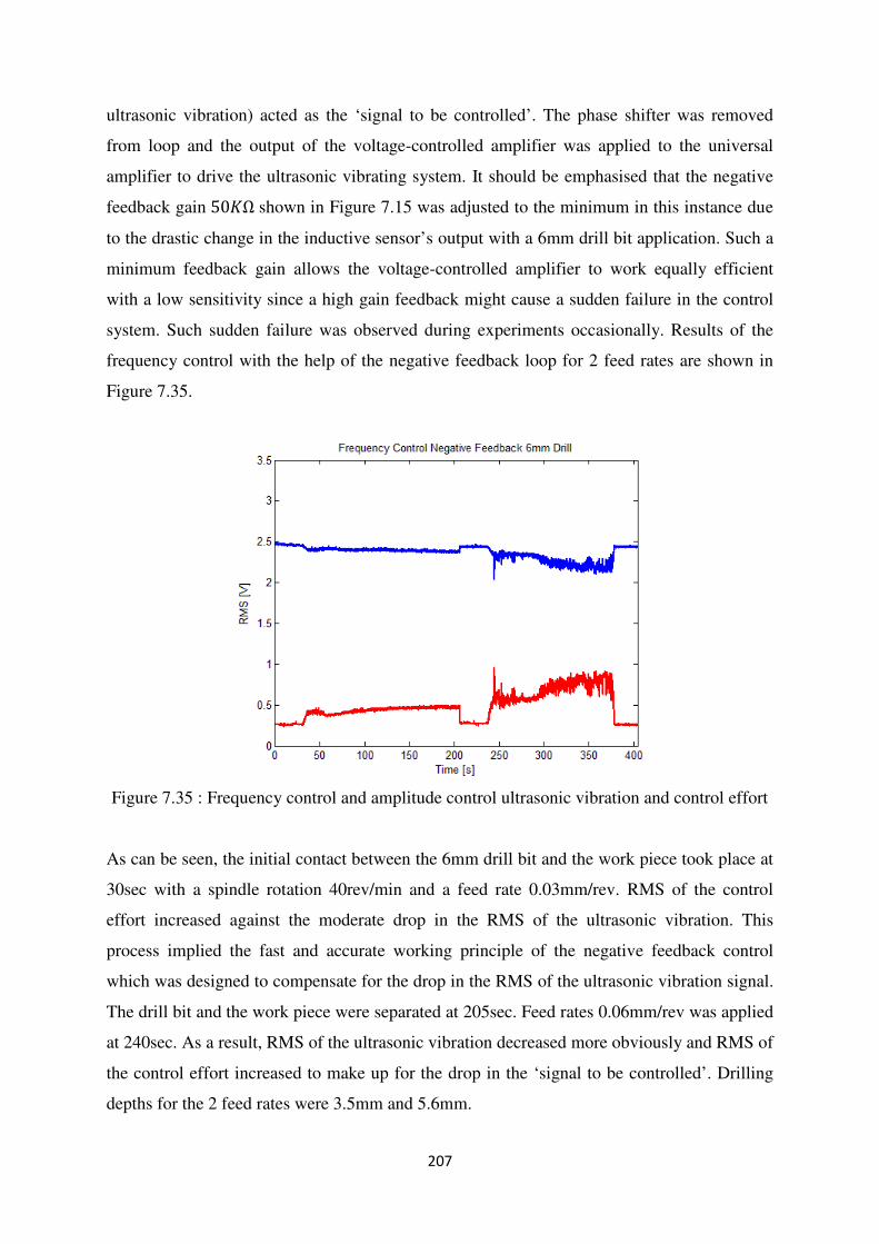
207
ultrasonic vibration) acted as the ‘signal to be controlled’. The phase shifter was removed
from loop and the output of the voltage-controlled amplifier was applied to the universal
amplifier to drive the ultrasonic vibrating system. It should be emphasised that the negative
feedback gain 50�Ω shown in Figure 7.15 was adjusted to the minimum in this instance due
to the drastic change in the inductive sensor’s output with a 6mm drill bit application. Such a
minimum feedback gain allows the voltage-controlled amplifier to work equally efficient
with a low sensitivity since a high gain feedback might cause a sudden failure in the control
system. Such sudden failure was observed during experiments occasionally. Results of the
frequency control with the help of the negative feedback loop for 2 feed rates are shown in
Figure 7.35.
Figure 7.35 : Frequency control and amplitude control ultrasonic vibration and control effort
As can be seen, the initial contact between the 6mm drill bit and the work piece took place at
30sec with a spindle rotation 40rev/min and a feed rate 0.03mm/rev. RMS of the control
effort increased against the moderate drop in the RMS of the ultrasonic vibration. This
process implied the fast and accurate working principle of the negative feedback control
which was designed to compensate for the drop in the RMS of the ultrasonic vibration signal.
The drill bit and the work piece were separated at 205sec. Feed rates 0.06mm/rev was applied
at 240sec. As a result, RMS of the ultrasonic vibration decreased more obviously and RMS of
the control effort increased to make up for the drop in the ‘signal to be controlled’. Drilling
depths for the 2 feed rates were 3.5mm and 5.6mm.

208
Such an improved control result revealed the effectiveness of the negative feedback control.
The voltage-controlled amplifier worked to react against the drop in the RMS of the
ultrasonic vibration and provided the ultrasonic vibrating system with more voltage to
compensate for the energy loss at the tip of the 6mm drill bit during vibro-impact.
Nevertheless, such superior control results could be attributed to the low Q factor of the
ultrasonic vibrating system as the resonant frequency shift during vibro-impact was small
which implied little drop in the amplitude in the frequency-amplitude characteristic. In
addition, nonlinearity was hardly developed with the application of a low feed rate and a low
spindle rotation with a low Q factor oscillating system. The increased voltage supply to a 4-
rings piezoelectric transducer was able to maintain the ultrasonic vibration at a desired level
during machining.
Figure 7.36 : Frequency control with amplitude control force versus conventional drilling
In comparison with the fixed frequency control, the ultrasonic vibrating system with the help
of the amplitude control system was able to deal with both feed rates and considerable
drilling depths. Therefore, remarkable force reductions during drilling for both feed rates
were expected. Results are shown in Figure 7.36. The initial contact of the 6mm drill bit with
the work piece happened at 15sec. Due to the participation of the amplitude control,
Ultrasonically Assisted Drilling (UAD) lasted for 90secs with a 40 rev/min spindle rotation
and a 0.03mm/rev feed rate. The steady thrust force during this process is less than 5�. At
105sec, both the frequency generator and the negative feedback control system were switched

209
off and the ultrasonic vibration vanished. Steady feed force turned into nearly 40� as a result
of the Conventional Drilling (CD). Control system was turned on after the separation of the
drill bit and the work piece and a higher feed rates 0.06mm/rev was applied at 235sec. As
soon as the Kistler dynamometer’s output signal became stable, the control system was
turned off. As a result, the thrust force immediately climbed up to a higher level 70�. Such
phenomenal force reductions for both feed rates seemed to correspond to the results shown in
Figure 7.35. A strong ultrasonic vibration existence at the tip of the 6mm drill bit during
drilling was implied. In addition, certain regular waveform of the 6mm drill bit during
machining was confirmed. In other words, RMS of the ultrasonic vibration at the end of
aluminium adaptor is a reliable observation point and can be treated as a ‘signal to be
controlled’ source.
7.3.2.3 Mechanical Feedback
Figure 7.37 : Mechanical feedback controlled ultrasonic vibration and control effort
Mechanical feedback control employs the actual ultrasonic vibration measured by an
inductive sensor as both the ‘actuating signal’ and the ‘signal to be controlled’. The aim of
this strategy is to maintain the ultrasonic vibration at the tip of a 6mm drill bit at a constant
during drilling through keeping the ultrasonic vibration at the end of the adaptor constant
based on the assumption that vibrations obtained from two positions are proportional. Since
mechanical feedback measures and controls the mechanical vibration directly, it is supposed
to present the overall best results. The operational procedure is that the phase shifter was

210
manually adjusted in order to bring the RMS of the ultrasonic vibration at the end of the
aluminium adaptor to the resonance. After this the potential meter ‘50�Ω’ shown in Figure
7.15 connected between the negative port of the offset amplifier OP07 and the output ‘���’
was tuned to the minimum. Such adjustments prevented the voltage-controlled amplifier’s
sudden failure due to the drastic change in the inductive sensor’s output during drilling. Then
the potential meter marked as ‘50�Ω’ connected between 12� and earth was adjusted until
both the voltage-controlled amplifier’s output (control effort) and the inductive sensor’s
output presented peak values. During drilling, the phase shifter and each element in the
negative feedback were fixed. Results of the mechanical feedback control are shown in
Figure 7.37.
The red curve represents the RMS of the control effort and the blue line stands for the RMS
of the ultrasonic vibration measured at the end of the adaptor. An ultrasonic vibration level
2.45� was obtained with a control effort RMS 0.3� . As can be seen, the initial contact
between the 6mm drill bit and the work piece happened at 15sec with a 0.03mm/rev feed rate
and a 40rev/min spindle rotation. As the drill bit penetrated deeper into the work piece, the
ultrasonic vibrating system required more energy to deal with the energy loss on the 6mm
drill bit tip. RMS of the control effort increased from 0.3� to 0.5�. Meanwhile, RMS of the
ultrasonic vibration was maintained perfectly at a constant. At 195sec, the drill bit and the
work piece were separated with a recovery of both the RMS in the ultrasonic vibration and
the control effort. At 225sec, a higher feed rate 0.06mm/rev was applied. Ultrasonically
Assisted Drilling (UAD) lasted for 140secs with the control effort increased from 0.3� to
0.7� which was twice as high as the control effort of the previous feed rate. RMS of the
ultrasonic vibration slightly decreased as the 6mm drill bit was engaged deeper into the work
piece but still can be kept at a constant level. For both feed rates, the control effort climbed
up gradually against the change in the inductive sensor’s output. In comparison, mechanical
feedback shows a superior control over the frequency control with the help of the negative
feedback shown in Figure 7.35. This emphasised the importance of the employment of phase
control rather than frequency control. For the same feed rate, the phase-amplitude
characteristic presents a more gently sloping peak than the frequency-amplitude characteristic
even though the Q factor of the ultrasonic vibrating system was reasonably low. It should be
emphasised that the resonant frequency has been monitored; the maximal change in the
resonant frequency was no more than 0.2��� which hardly altered the phase in the phase-

211
amplitude characteristic of the ultrasonic vibrating system. Drilling depth for 2 feed rates
were 3.7mm and 5.6mm.
Figure 7.38 : Mechanical feedback force reduction versus Conventional Drilling (CD)
In order to examine the existence of the ultrasonic vibration on the tip of the 6mm drill bit
during machining, the feed force was monitored and results are shown in Figure 7.38. The
initial contact with a 0.03mm/rev feed rate and a 40rev/min rotation happened at 25sec and
Ultrasonically Assisted Drilling (UAD) process lasted for 90secs until the feed force
stabilised. The thrust force level during this process was around 5� . At 115sec, the
mechanical feedback control system was switched off which resulted in a sudden increase in
the thrust force to 40�. This process showed the transition from the Ultrasonically Assisted
Drilling (UAD) to the Conventional Drilling (CD). The drill bit and the work piece were
separated at 195sec and the control system was turned on. A higher feed rate 0.06mm/rev was
applied at 240sec and feed force increased to 8� . This Ultrasonically Assisted Drilling
(UAD) process lasted until 315sec with a switch-off of the mechanical feedback control. As a
result, Conventional Drilling (CD) took place which produced a nearly 75� feed force. Such
tremendous force reductions from the Conventional Drilling (CD) to the Ultrasonically
Assisted Drilling (UAD) for both feed rates proved a strong ultrasonic vibration at the tip of
the 6mm drill bit.

212
7.3.2.4 Current Feedback
Figure 7.39 : Current feedback controlled ultrasonic vibration, current and control effort
Current feedback uses a current probe which is placed between the universal matchbox
(transformer) and the ultrasonic transducer to measure the current � flowing through the
pizeoceramic rings and considers it as both the ‘actuating signal’ and the ‘signal to be
controlled’. This strategy aims at maintaining the ultrasonic vibration at the end of the
adaptor which is proportional to the ultrasonic vibration on the tip of a 6mm drill bit at a
constant level during drilling. This is done through stabilising the current �. Since current
feedback controls the mechanical vibration in an indirect way, the effectiveness of the control
entirely relies on the dynamic coupling between the current and the mechanical vibration
characteristics. The experimental procedure is the phase shifter was adjusted to reach the
current resonance and then the potential meter marked as ‘50�Ω’ shown in Figure 7.15 was
adjusted to allow the maximum gain (since the electrical characteristics are obtained at a
distance from the machining zone therefore the changes are small) in the negative feedback
loop. This negative feedback gain values depend on the change in the ‘signal to be
controlled’. It was experimentally found that the drop in the current signal was not as drastic
as the ultrasonic vibration as the electrical parameters were located at a distance from the
machining zone which was affect less than the mechanical characteristics. The other ‘50�Ω’
potential meter in Figure 7.15 was adjusted until both the output of the voltage-controlled
amplifier (control effort) and the output of the current probe reached resonance. It should be
emphasised, being similar to a 3mm drill bit application, neither a band-pass filter nor a

213
Butterworth filter was employed to tackle the ambiguity characteristic of the current signal
during drilling. Each element in the current feedback remained unchanged during drilling.
Results of the current feedback are presented in Figure 7.39.
Figure 7.39 presents the oscilloscope readings of the drilling experiment with the current
feedback control system on a 6mm drill bit. Blue curve represents the RMS of the ultrasonic
vibration, pink curve stands for the RMS of the current and red curve shows the RMS of the
control effort. A RMS of the ultrasonic vibration 2.75� was obtained with a RMS of 0.38�
for control effort and a RMS of 0.85� for current. Same as the previous experiment, 2 feed
rates had been applied which were: 0.03mm/rev (20sec) and 0.06mm/rev (245sec). For the 2
intervals when the feed rates were applied, the increase in the control effort could be
observed. This increase in the control effort demonstrated the control system was working to
compensate for the changes in the current sensor’s output which was caused by the applied
load. Current sensor’s output, on the other hand, slightly dropped during drilling but still
could be maintained at a desired level. This showed the efficiency of the control system as it
was able to stabilise the amplitude of the ‘signal to be controlled’. In terms of the inductive
sensor’s output, it demonstrated obvious decreases especially for the high feed rate which
implied a weakened coupling between the current and the mechanical vibration in reality for
a 6mm drill bit application. In a better interpretation, although stabilising the ultrasonic
vibration through keeping the current is still an effective method, current feedback worked
not efficient as mechanical feedback. Instead, it has a comparable performance with the
frequency control with help of the negative feedback control system. Resonant frequency
shift during the Ultrasonically Assisted Drilling (UAD) process was no more than 0.2���
which indicated little phase change. Drilling depth for 3 feed rates were 3.7mm and 6.4 mm.
The force reduction experiment for the current feedback has been executed. Results are
shown in Figure 7.40. 2 feed rates were executed with current feedback which happened at
20sec and 230sec. When the Ultrasonic Assisted Drilling (UAD) process stabilised, the
current feedback control was turned off which occurred at 110sec and 310sec. As a result, the
steady feed force increased significantly to a higher level. Therefore, considerable force
reductions for 2 feed rates indicated a strong ultrasonic vibration at the tip of the 6mm drill
bit. Current feedback control worked efficiently to maintain the ultrasonic vibration on the tip

214
of the 6mm drill bit during vibro-impact through stabilising the current and hence is a reliable
control strategy.
Figure 7.40 : Current feedback force reduction versus Conventional Drilling (CD)
7.3.2.5 Power Feedback
Figure 7.41 : Power feedback controlled ultrasonic vibration, power and control effort
Power feedback employs a power sensor shown in Figure 7.7 (manufactured in the ultrasonic
machining laboratory, Loughborough University) to measure the scaled instantaneous power
and applies it as the ‘signal to be controlled’ in negative feedback loop. Current flows
through the piezoelectric transducer still acts as the ‘actuating signal’ to form the positive

215
feedback. This strategy aims at maintaining the ultrasonic vibration at the end of the adaptor
which is in proportion to the ultrasonic vibration on the tip of the 6mm drill bit at a constant
level through stabilising power. The experimental procedure is the phase shifter and potential
meter marked as 100�Ω and 50�Ω in Figure 7.7 were properly adjusted. The 50�Ω
potential meter shown in Figure 7.15 had been tuned to achieve the maximum gain (since the
electrical characteristics are obtained at a distance from the machining zone therefore the
changes are small) and the other 50�Ω potential meter was adjusted to reach the power
resonance which was designed to have a similar level as the RMS of the current in the current
feedback. Each element in the power feedback system remained fixed during drilling. Results
of the power feedback are showed in Figure 7.41.
Blue curve represents the RMS of the ultrasonic vibration measured by an inductive sensor,
pink curve stands for the RMS of the scaled instantaneous power measured by a power sensor
and red curve is the RMS of the control effort which is the output of the voltage-controlled
amplifier. A RMS 2.7� of the ultrasonic vibration, a RMS 0.38� of the control effort
together with a RMS 0.89� of the instantaneous power was obtained initially. In this
instance, 2 feed rates 0.03mm/rev and 0.06mm/rev were applied which happened at 15sec
and 230sec. Control effort can be clearly observed which indicated that the power feedback
control was working to compensate for the decrease in the RMS of the instantaneous power.
RMS of the power sensor’s output indicated a nearly constant level for both feed rates which
required a little increase in the control effort. In terms of the inductive sensor’s output, there
were more obvious decreases for 2 feed rates than the other 2 feedbacks. This implies a
weaker coupling between the mechanical vibration characteristic and the instantaneous power
signal than the current signal. Resonant frequency monitored during the power feedback
controlled Ultrasonically Assisted Drilling (UAD) showed no more than 0.2��� which
meant little change in the phase in phase-amplitude characteristics. Drilling depth for 2 feed
rates were 3.6mm and 5.9mm.
Force reductions for the power feedback are illustrated in Figure 7.42. 2 feed rates
0.03mm/rev and 0.06mm/rev were examined which happened at 20sec and 220sec. Power
feedback controlled ultrasonic vibrating system was switched on initially and after certain
depth of Ultrasonically Assisted Drilling (UAD) with a stabilisation of the Kistler
dynamometer’s output, control system was turned off. As can be observed, tremendous force

216
reductions indicated strong ultrasonic vibrations on the tip of the 6mm drill bit during vibro-
impact. The ultrasonic vibration amplitude can be kept through keeping the RMS of the
instantaneous power at a constant level. Being similar to the current feedback, this remote
control strategy also emphasises the convenience and feasibility of the employment of the
instantaneous power as a feedback signal, although this remote control strategy might not be
as effective as the mechanical feedback.
Figure 7.42 : Power feedback force reduction versus Conventional Drilling (CD)
7.3.2.6 Summary
Being similarly to the investigation of a 3mm drill bit application, in order to analyse the
efficiency of different control strategies more clearly, the maximum deflection in RMS of the
ultrasonic vibration from the desired levels, drilling force reductions for each feed rate for a
6mm drill bit application have been shown in Table 7.4 and Table 7.5.
As can be seen in Table 7.4, maximum deflection of the RMS of the ultrasonic vibration
presents tremendously large values for both feed rates for the fixed frequency control which
indicates a failure. Therefore, no force reduction was observed. With the help of the
amplitude control system, RMS of the ultrasonic vibration at the end of the transducer can be
maintained at a desired level even though a high feed rate 0.06mm/rev shows a greater
deflection. Consequently, force reduction for both feed rates is phenomenal shown in Table
7.5. The improvement of the control with the help of negative feedback indicates a low Q

217
factor of the ultrasonic vibrating system. In other words, sufficient voltage supply is able to
keep the ultrasonic vibration at a desired level during vibro-impact regardless of a small
resonant frequency shift.
Table 7.4 : Maximum deflection in RMS of the ultrasonic vibration of a 6mm drill bit
application
Strategy
Deflection
Frequency
Control
Freq+Amp
control
Mechanical
Feedback
Current
Feedback
Power
Feedback
0.03mm/rev
93.4%
3.7%
2.5%
4.0%
8.2%
0.06mm/rev
95.7%
11.6%
0.1%
11.0%
17.3%
Table 7.5 : Feed force reduction of a 6mm drill bit application
Strategy
Reduction
Freq+Amp
control
Mechanical
Feedback
Current
Feedback
Power
Feedback
0.03mm/rev
89.3%
88.0%
86.3%
86.0%
0.06mm/rev
88.2%
90.7%
88.0%
87.7%
For 3 autoresonant control strategies, experiments reveal that mechanical feedback shows an
overall best performance with a minimum deflection in the RMS of the ultrasonic vibration
from the desired levels shown in Table 7.4. Meanwhile, considerable force reductions shown
in Table 7.5 for 2 feed rates are observed for mechanical feedback. This superior control can
be ascribed to that mechanical feedback employs the ultrasonic vibration at the end of the
transducer as the ‘signal to be controlled’ and controls it directly. In contrast, current
feedback shows a worse control in terms of the deflection in the RMS of the ultrasonic
vibration at the end of the transducer and the force reduction for 2 feed rates. To this point, it
can be concluded that the characteristic of the current is related to the ultrasonic vibration.
However, compared with the application of a 3mm drill bit, an increased sized drill bit seems

218
to have more effect on the current feedback control. Therefore, such an indirect control
strategy still realises the remote control possibility for the industrial use but not efficient as
the mechanical feedback. Power feedback presents an overall worst performance compared
with the other 2 strategies in the sense of the maximal deviation in the RMS of the ultrasonic
vibration. Again, this control strategy’s principle is debatable since the target of negative
feedback is to increase the supplied power to the ultrasonic vibrating system rather than
stabilise it. It’s strongly suggested a modification is executed to increase the supplied power
during power feedback control. Nonetheless, considerable force reductions of the power
feedback show it has a comparable control to the current feedback.
Generally speaking, by observing the results shown in Table 7.4 and Table 7.5, the
improvement of using autoresonant control from the fixed frequency control is remarkable,
especially dealing with high Q factor oscillating systems. In order to explore which control
strategy presents the overall best performance, surface roughness examination which is a
direct informative reflection of control will be presented.
7.4 Holes Surface Roughness Examination
In order to explore the impact of different control strategies impose on the aluminium plates,
holes have been produced for both diameters of drill bit 3mm and 6mm with several feed
rates (0.03mm/rev and 0.09mm/rev for a 3mm drill bit, 0.06mm/rev for a 6mm drill bit) and a
fixed spindle rotation 40 rev/min. Theoretically, a number of measurements can be executed
on the specimens in order to evaluate the holes quality, including roundness, burr formation,
tool wear, surface roughness etc. However, for such handmade ultrasonic vibrating systems,
circularity measurement is not able to reveal the advantages and the disadvantages of each
control strategies because it needs a high precision ultrasonic vibrating system setup. Instead,
surface roughness reflects the direct information of the ultrasonic drilling with different
control strategies. Therefore, the surface roughness experiments have been carried out.
The aluminium specimens have a thickness 15mm, 2 diameters of drill bits were used to
produce through holes with different control strategies. After that, holes have been milled
through the middle and the inner surface quality of the grooves was measured. A
TALYSURF CLI 2000 machine [84] was available in the Metrology Laboratory in
Loughborough University which was used to perform the surface roughness test. It should be

219
noted that the measurement length for each groove was 12 mm and for each case the
measurement settings remain same for each set of experiment. Surface roughness results for a
3mm drill bit and a 6mm drill bit can be seen in the following.
7.4.1 A 3mm Drill Bit Surface Roughness
Figure 7.43 : Surface roughness of a 3mm drill bit with a 0.03mm/rev feed rate
Table 7.6 : Surface roughness test with a 0.03mm/rev and a 40rev/min of a 3mm drill bit
application
Strategy �� (��) �� (��) �� (��) �� (��) �� (��) �� (��)
Conventional 5.527 46.543 12.585 13.695 6.5487 26.28
Frequency
Control 4.7738 49.565 12.413 12.679 5.9565 25.093
Current
Feedback 1.9024 22.905 5.3005 6.7074 2.4411 12.008
Power
Feedback 1.7453 15.087 4.3032 4.6882 2.1402 8.9914
Mechanical
Feedback 1.5337 21.218 3.7739 5.8589 2.0575 9.6328
Figure 7.43 shows the holes surface roughness profiles deviations from their ideal surfaces
produced by a 3mm drill bit with a feed rate 0.03mm/rev and a rotation 40rev/min with
different control strategies. (a) represents the surface roughness of the Conventional Drilling

220
(CD) (non-ultrasonic), (b) shows the fixed frequency control, (c) demonstrates the current
feedback, (d) stands for the power feedback and (e) is the mechanical feedback. Horizontal
axis is the groove length and vertical axis is the surface profiles. As can be seen, the surface
roughness profiles were considerably improved with an application of the autoresonant
control as the curves show smaller deviations. Parameters of the surface roughness for the
holes produced by different control strategies can be seen in Table 7.6.
Figure 7.44 : Surface roughness of a 3mm drill bit with a 0.09mm/rev feed rate
�� means the arithmetic average of the absolute values which is the most commonly used
measurement parameters. �� is the range of the collected roughness data points. �� is the
maximum peak height and �� is the maximum valley depth. �� is the root mean squared
values of evaluated data points. �� is the average distance between the highest peak and
lowest valley each sampling length. All the measurement parameters have units ��. As can
be seen, the most commonly used parameter �� indicates an overall maximum deviation of
data points for the Conventional Drilling (CD) and a minimum deviation for the mechanical
feedback control. Current feedback and power feedback show a slightly larger deviation, but
improvement of the autoresonant control produced holes quality is remarkable.
Figure 7.44 shows the surface roughness profile of a 3mm drill bit produced holes with
different control strategies for a 0.09mm/rev feed rate and a 40rev/min rotation of the spindle.

221
(a), (b), (c), (d) and (e) have the same meanings as the 0.03mm/rev feed rate. As can be seen
in Table 7.7, the power feedback shows an overall smallest deviation �� where Conventional
Drilling (CD) exhibits the maximum. The current feedback and the mechanical feedback
seem slightly worse than the power feedback in the surface roughness evaluation however
still show superiority over the Conventional Drilling (CD) and the fixed frequency control.
This emphasises the advantages of the employment of the autoresonant control even with a
high feed rate.
Table 7.7 : Surface roughness test with a 0.09mm/rev and a 40rev/min of a 3mm drill bit
application
Strategy �� (��) �� (��) �� (��) �� (��) �� (��) �� (��)
Conventional 6.0497 58.745 13.86 15.859 7.4142 29.719
Frequency
Control 4.9983 53.675 12.632 15.032 6.3811 27.664
Current
Feedback 2.8994 33.697 7.5257 9.0908 3.7056 16.616
Power
Feedback 2.1256 24.319 5.026 7.9691 2.7001 12.995
Mechanical
Feedback 3.4921 27.499 7.6466 10.362 4.2895 18.008
7.4.2 A 6mm Drill Bit Surface Roughness
Figure 7.45 : Surface roughness of a 6mm drill bit application with a 0.06mm/rev feed rate

222
Figure 7.45 shows the surface roughness profile of a 6mm drill bit produced holes with
different control strategies for a 0.06mm/rev feed rate and a 40rev/min rotation of the spindle.
(a), (b), (c), (d) and (e) represent the control strategies same as Figure 7.43 and Figure 7.44.
As can be seen in Table 7.8, mechanical feedback, current feedback and power feedback
show a comparable deviation �� where the Conventional Drilling (CD) or even the fixed
frequency control exhibits a several times larger value. This emphasises the advantages of the
employment of the autoresonant control even with an increased diameter drill bit.
Table 7.8 : Surface roughness test with a 0.06mm/rev and a 40rev/min with a 6mm drill bit
Strategy �� (��) �� (��) �� (��) �� (��) �� (��) �� (��)
Conventional 8.0287 95.593 18.396 22.926 10.158 41.322
Frequency
Control 6.5282 48.596 15.039 14.351 7.7196 29.39
Current
Feedback 3.4254 35.18 9.3441 11.896 4.4622 21.24
Power
Feedback 3.3696 27.542 8.8707 10.097 4.2268 18.968
Mechanical
Feedback 3.4742 35.105 8.2785 13.167 4.507 21.445

223
Chapter Eight Conclusions and Future Work
Ultrasonically Assisted Drilling (UAD) has won recognition in industrial applications due to
its prominent advantages over Conventional Drilling (CD), i.e. tremendous force reduction,
burr elimination, shorter chip formation, surface roughness and circularity improvement,
strong ability to machine difficult-to-cut materials etc. Analysis on the dynamics of a
distributed parameter model suggests a simplified 2-DOF model which consists of 2 sets of
spring-mass-damper as a replacement of a 2-step electromechanical ultrasonic transducer
used in experiments. Despite resonant frequencies of the 2-step electromechanical transducer
and the 2-DOF model are different, an agreement of the ultrasonic vibration amplitude at the
end of the 2nd
step concentrator confirms the feasibility and possibility to employ such a
simple 2-DOF model in numerical simulation. In order to complete an ultrasonic vibrating
system, an applied load model with a Kelvin-Voigt form has been developed, parameters
have been computed and confirmed according to a vibro-impact experiment performed on an
Ultrasonically Assisted Broaching (UAB) experiment. Consistency of the simulation results
and the experimental results verifies the accuracy of the applied load model.
An autoresonant control feedback system which combines the phase control and the
amplitude control has been created in Matlab-Simulink. 3 feedback control strategies namely
mechanical feedback control, current feedback control and power feedback control have been
executed and compared. A Butterworth filter with a proper bandwidth has been selected to
perform the current feedback and the power feedback. By changing the applied load
parameters, mechanical feedback shows an overall best result over current feedback and
power feedback. However, the difference between these three feedback control strategies
remains small. The explanation for such little difference could be that the drill bit effect is
ignored during numerical simulation. Frankly speaking, efficiency of the electrical feedback
control entirely depends on the dynamic coupling between the electrical parameters and the
mechanical vibration characteristics. Currently, formulae which describe the electrical current
and the mechanical state are only available in piezoceramics supplier’s technical
specification. The linear operational interval of the piezoelectric transducer might be changed
in reality depending on the piezoceramic material etc. This implies a simplified process of the
piezoelectric transducer in numerical simulation. Nonetheless, the autoresonant controlled
ultrasonic vibration level during change in the applied load presents a superior performance

224
in comparison with the fixed frequency control and the non-ultrasonic machining which react
sensitively to the applied load. It should be emphasised that in numerical simulation a tool is
not attached due to a complex dynamics and geometry of a drill bit creates during the applied
load which will complicate the simulation process.
In order to verify the numerical results and investigate the drill bit effects on the autoresonant
control, experiments have been performed. A prototype autoresonant control system has been
designed and manufactured and 2 dimensions of drill bits 3mm and 6mm in diameter were
employed to execute the Ultrasonically Assisted Drilling (UAD) experiments. Different feed
rates in combination with a fixed spindle rotation speed were applied to 3 control strategies.
A completed investigation reveals that the mechanical feedback shows the overall superior
control over the other 2 feedback control strategies. This emphasises the importance and
efficiency of using the direct ultrasonic vibration information which is obtained by a
mechanical sensor placed in the machining zone. 2 dimensions of drill bits applications on
the autoresonant control present the highest efficiency of maintaining the RMS of the
ultrasonic vibration in the mechanical feedback. Although the ultrasonic vibration at the tip of
a drill bit is unavailable during machining, it has been experimentally proved that the
ultrasonic vibration at the end of the concentrator is proportional to the vibration at the tip of
a drill bit due to a regular waveform of an ultrasonic vibrating system. In industrial
applications, the inductive sensor could be effectively employed as a replacement of the laser
vibrometer due to its low cost. In order to ensure the persistency and safety of the
Ultrasonically Assisted Drilling (UAD) process, the inductive sensor can be placed anywhere
(apart from the nodal point) along the direction of the waveguide where is far from the
machining zone. The ultrasonic vibration level on the tip of the drill bit could be maintained
through keeping the inductive sensor’s output stable due to the fact that the ultrasonic
vibrating system conforms to a regular waveform at resonance.
In comparison, electrical feedback use a current sensor or a power sensor to measure the
electrical characteristics of the piezoelectric transducer then employ them as the ‘actuating
signal’ and the ‘signal to be controlled’ in the feedback loop. Therefore, electrical feedback
reflects the mechanical vibration in an indirect way which inevitably worsens the control
accuracy of the ultrasonic vibration. Furthermore, the electrical parameters are less affected
by the machining zone compared with mechanical characteristics which also explains the
reduced efficiency of the electrical feedback control during maintaining. Ultrasonically

225
Assisted Drilling (UAD) experiments showed that the power feedback exhibited a slightly
worse control than the current feedback and this deterioration was aggravated as the diameter
of a drill bit increased. Generally speaking, power feedback shows the lowest efficiency in
keeping the ultrasonic vibration level and the explanation is the ultrasonic vibrating system
requires more power during vibro-impact process. However, power feedback is designed to
keep the power at a constant level which is debatable. It is therefore strongly recommended
that more power should be produced in the power feedback control in order to compensate
the the energy loss and stabilise the mechanical vibration. Current feedback, on the other
hand, aims to stabilise the current by increasing the control effort which results in an overall
power increase. It should be emphasised that being contrary to the numerical simulation, the
electrical feedback required no Butterworth filters to tackle the ‘confusion’ problem (one
phase corresponds to several vibration regimes). This conflict reveals the difference between
the theory and the practice. The piezoelectric effect is a complicated process in reality which
can be affected by many factors. Whereas, a formula describes the mechanical state and the
electrical current has been employed in the numerical simulation which essentially simplify
the piezoelectric effect. Surface roughness profiles for a 3mm drill bit and a 6mm drill bit
generally conforms to the experimental results except certain particular feed rates.
The limitation of the autoresonant control technology is the driving power of the ultrasonic
vibrating system. As explained that a 2-piezoceramic rings transducer used for the application
of a 3mm drill bit was insufficient to drive a 6mm drill bit. Therefore, a more powerful
transducer with 4-piezoceramic rings acting as the actuating elements was employed for the
application of a 6mm drill bit. Even though, a feed rate higher than 0.06mm/rev in
combination with a spindle rotation 40rev/min led to a failure in control. The acoustic power
handling capacity of a radiating transducer is limited by several factors including the dynamic
mechanical strength of the ceramic, the reduced efficiency due to the dielectric loss and the
mechanical loss, the depolarisation of the ceramic which disable the piezoelectric rings to
benefit more vibrations from increased supplied voltage and therefore results in saturation.
One of the possible solutions to tackle the power limitation of the piezoelectric transducer is
to add more piezoceramic rings to drive the ultrasonic transducer. However, it’s been
explored in experiment that a 4-ring piezoelectric transducer does not indicate a doubled
power compared with a 2-ring piezoelectric transducer. Alternatively, more powerful
piezoceramic rings can be employed to such as PZT-8. Ideally, an increased voltage supply to

226
the actuation elements should generate stronger ultrasonic vibrations at the tip of a tool.
Therefore, it is strongly recommended the linear operation voltage interval of a piezoelectric
transducer should be extended. In order to achieve this, another option is to replace the
universal amplifier and the universal matchbox (transformer) with a valve amplifier which
allows operating at a higher voltage without any waveform distortion. As introduced before,
the universal amplifier’s linear operational zone is ±70� and any signal output exceeds this
range will be truncated. According to experiments, such a narrow zone limits the effective
control efforts supplied to the universal matchbox (transformer). The autoresonant control
realises the possibility of maintaining the nonlinear resonant mode of oscillations caused by
the applied load in ill-defined and time changing conditions where the fixed frequency
control or even an adjusted frequency control seems insufficient. In order to show the high
efficiency of the autoresonant control technique, a high Q factor ultrasonic vibrating system
is strongly recommended.
In addition to the limitation of the supplied power to the piezoelectric transducer, an
improved design of a drill bit is suggested. The drill bits used in the autoresonant control
during Ultrasonically Assisted Drilling (UAD) are conventional, standard, heavy duty drill
bits with regular helix angles and high point angles which have stronger cutting edges and
produce narrow chips, such drill bits are used in materials that have been hardened or
extremely tough. Such drill bits were able to develop a considerable force reduction during
autoresonant control on the specimens of aluminium with hardness 77HV. However, it was
explored that when the hardness of the aluminium alloy was increased or different materials
were applied, the autoresonant control was not so efficient. This is partially due to the
limitation on the supplied power to the ultrasonic transducer and the changed material
properties, i.e. hardness etc. Another important reason is the geometry of the drill bits.
Therefore, it is also a subject of interest to investigate different geometry of drill bits to
examine the tool effect on the autoresonant control. A successful design of a drill bit could
improve the efficiency and robustness of an autoresonant control system.
An optimization on the universal matchbox for the application of a 6mm drill bit on a 4-
piezoring ultrasonic transducer has been executed and the results are promising and
interesting. The idea of the optimization process is to increase the gap between 2 ferrite cores
until the maximal ultrasonic vibration amplitude is achieved with a fixed input signal to the
universal amplifier. Experimental results indicate that an air gap ∆= 2.5�� is the optimal

227
gap distance which develops the largest ultrasonic vibration, a nearly �2 phase shift between
the voltage and the current across the universal matchbox (transformer), maximal voltage and
maximal current as well as a peak power. Analysis shows that the optimal air gap is able to
cancel the phase different between the voltage and the current in an LC circuit which is a
simplified form of the universal matchbox (transformer) and the ultrasonic transducer.
Therefore, a maximal energy transfer from the source to the piezoelectric transducer is
achieved. This enables the ultrasonic transducer to work at the most efficient regime at
resonance.
For each ultrasonic vibrating system, the universal matchbox (transformer) optimization
process is critical and indispensable as the effective inductance of the universal matchbox
(transformer) will change considerably as the air gap develops which will inevitably change
the behaviour of the ultrasonic vibrating system in terms of resonant frequency, vibration
amplitude, driving voltage etc. It should be mentioned that at the end phase of the project, a
more powerful amplifier module MF450 was purchased to replace the defected MF200
module. The new amplifier module proves to deliver extremely powerful signal to the
ultrasonic transducer. The driving voltage for the ultrasonic transducer easily exceeds 3000
volts peak-to-peak. As a result, the piezoceramic rings seems not to reject such a high voltage
as observed in experiments. Therefore, it is strongly recommended to explore a bigger size
drill bit for the autoresonant control. Moreover, it is also worth to explore the maximal
working voltage of the piezoceramic rings.

228
References
[1] Abboud, N.N., Wojcik, G.L., Vaughan, D.K., J. Mould, D.J. Powell and L. Nikodym
(1998). Finite Element Modelling for Ultrasonic Transducers. Proceedings – SPIE the
international society for optical engineering. Issue 3341: pp. 19-42.
[2] Alam, K., Mitrofanov, A.V. and Silberschmidt, V.V. (2011). Experimental
investigations of forces and torque in conventional and ultrasonically assisted drilling
of cortical bone. Medical Engineering & Physics. Vol.33: pp. 234-239.
[3] Anton, H. and Rorres, C. (2000). Elementary Linear Algebra.(Applications Version),
8th
Edition, John Wiley. (Chpater 7, hard copy)
[4] Azarhoushang, B. and Akbari, J. (2007). Ultrasonic-assisted drilling of Inconel 738-
LC. International Journal of Machine Tools&Manufacture 47: pp. 1027-1033.
[5] Astashev, V.K. (1981). Calculation of rod concentrators with a nonlinear load.
Soviet Physics-Acoustics 27(6).
[6] Astashev, V.K. and Babitsky, V.I. (1998). ‘Ultrasonic cutting as a nonlinear (vibro-
impact) process’. Ultrasonics Vol. 36 (n. 1-5): pp. 89-96.
[7] Astashev, V.K. and Babitsky, V.I. (2000). Dynamics and Control of Machines. Berlin,
Springer, ISBN: 3540637222.
[8] Astashev, V.K. and Babitsky, V.I. (2007). Ultrasonic Processes and Machines –
Dynamics, Control and Applications. Berlin, Springer, ISBN: 978-3-540-72060-7.
[9] Astashev, V.K. and Sakayan, A.R. (1967). Experimental investigation of the dynamics
of the vibrating system of an ultrasonic lathe. Mashinovedenie.Vol.4 (n.3-n.7). (in
Russian)

229
[10] Babitsky, V.I. (1992). Some Applications of Autoresonant Strongly Nonlinear
Vibratory Systems. Machine Vibration Vol.1 (n.2): pp. 110-119.
[11] Babitsky, V.I. (1995). Autoresonant mechatronic systems. Mechatronics. Vol.5: pp.
483-495.
[12] Babitsky, V.I. (1998). Theory of Vibro-Impact Systems and Applications. Berlin,
Springer. Revised translation from Russian, Moscow, Nauka, 1978.
[13] Babitsky, V.I. (2009). Autoresonant excitation and control of nonlinear vibration
modes. Physcon, Catania, Italy.
[14] Babitsky, V.I., Astashev, V.K. and Kalashnikov, A.N. (2004). Autoresonant control
of nonlinear mode in ultrasonic transducer for machining applications. Ultrasonics
42: pp. 29-35.
[15] Babitsky, V.I., Astashev, V.K. and Meadows, A. (2007). Vibration excitation and
energy transfer during ultrasonically assisted drilling. Journal of Sound and
Vibration 308: pp. 805-814.
[16] Babitsky, V.I., Kalashnikov, A.N. and Molodtsov, F.V. (2004). Autoresonant control
of ultrasonically assisted cutting. Mechatronics, Vol. 14 (n.1): pp. 91-114.
[17] Babitsky, V.I. and Sokolov, I.J. (2002). Autoresonance Control of Vibratory Systems.
The sixth international conference on Motion and Vibration Control. Saitama, Japan.
Japan Society of Mechanical Engineers: pp. 643-648.
[18] Babitsky, V.I. and Sokolov, I.J. (2007). Autoresonant homeostat concept for
engineering application of nonlinear vibration modes. Nonlinear Dyn 50: pp. 447-
460.
[19] Balamuth, L. (1964). Ultrasonic vibrations assist cutting tools. Metalwork. Prod.
108(24): pp. 75-77.

230
[20] Bogomolov, S. and Simson, E. (1981). Optimal design of ultrasonic concentrators.
Acoustical Journal. Vol.27 (4) (in Russian)
[21] Brehl, D.E. and Dow, T.A. (2008). Review of vibration-assisted machining. Precision
Engineering, Vol.32 Issure 3: pp. 153-172.
[22] Bruce, T. (1984). ‘Energy Methods’. Advanced Dynamics for Engineers. HRW Series
in Mechanical Engineering. United States of America: CBS College Publishing. ISBN
0-03-063366-4.
[23] Chern, G.L. and Liang, J.M. (2007). Study on boring and drilling with vibration
cutting. International Journal of Machine Tools&Manufacture 47: pp. 133-140.
[24] Chew, E.K (1988). Response of a rotating machine supported on nonlinear springs.
[25] Clifton, D., Imal, Y. and Mc-Geough, J.A. (1993). Some ultrasonic effects on
machining materials encountered in the offshore industries. In: Proceedings of the
30th International MATADOR Conference: pp. 119-123.
[26] Day, R.A. (1996). PVDF and Array Transducers. Lawrence Livermore National
Laboratory.
[27] Devine, J. (1985). Ultrasonically assisted metal removal. Source Book: American
Society for Metals, Fabrication of Composite Materials.
[28] Farago, F.T. (1980). Abrasive Methods Engineering. Industrial Press.Vol.2: pp. 480-
481.
[29] Farrer, J.O. (1948). USM. English Patent No. 602801
[30] Fuller, C.R., Elliott, S.J. and Nelson, P.A. (1996). Active Control of Vibration.
Academic Press INC, ISBN:0-12-269440-6.

231
[31] Gary, F.B. (1987). Book on Non-Traditional Manufacturing Processes. Marcel
Dekker, nc, New York: pp. 67-86 Chap 6.
[32] Ghahramani, B. and Wang, Z.Y. (2001). Precision ultrasonic machining process: a
case study of stress analysis of ceramic (��2�3). International Journal of Machine
Tools & Manufacture.Vol.41: pp. 1189-1208.
[33] Gilmore, R. (1990). Ultrasonic machining of ceramics. SME Paper.MS90-346 (12).
[34] Harlow, J.H. (2004). Electric power transformer engineering. CRC Press: pp.2-216.
ISBN 9780849317040.
[35] Kennedy, D.C. and Grieve, R.J. (1975). Ultrasonic machining – a review. Prod. Eng.
54(9): pp. 481-486.
[36] Kikuchi, Y. (1969). Ultrasonic transducers. Corona.
[37] Kremer, D. (1991). New developments on ultrasonic machining. SME Technical
Paper MR91-522: pp. 13.
[38] Kumabe, J. (1979). Vibratory Cutting. Jikkoyo Publisher, Tokyo(in Japanese).
[39] Kuo, K.L. (2009). Ultrasonic vibrating system design and tool analysis. Transactions
of Nonferrous metals Society of China. s225-s231.
[40] Lacalle, L.D. and Norberto, L. (2008). Ultrasonic assisted machining. SciTopics.
[41] Li, Z.C., Jiao, Y., Deines, T.W., Pei, Z.J. and Treadwell, C. (2005). Rotary ultrasonic
machining of ceramic matrix composites: feasibility study and designed experiments.
International Journal of machine Tools & Manufacture. Vol.45: pp. 1402-1411.
[42] Liang, Z.Q., Wu, Y.B., Wang, X.B. and Zhao, W.X. (2010). A new two-dimensional
ultrasonic assisted grinding (2D-UAG) method and its fundamental performance in

232
monocrystal silicon machining. International Journal of Machine Tools&Manufacture
50: pp. 728-736.
[43] Madan, V.P., submitted by Dolph, C.L. (1969). On Longitudinal Vibrations of a
Semi-Infinite Voigt-Kelvin Rod with Non-Uniform Viscoelastic Properties.Journal of
Mathematical Analysis and Applications 28, 88-92.
[44] Module 9, Non-conventional machining. Lesson 36 Ultrasonic Machining (USM).
Version 2 ME, IIT Kharagpur.
[45] Neppiras, E.A. (1956). Report on ultrasonic machining. Metalworking Prod. Vol.100
: pp. 1283-1288,1333-1336,1377-1382,1420-1424,1464-1468,1554-1560,1599-1604.
[46] Neppiras, E.A. (1964). Ultrasonic Machining and Forming. Ultrasonics for industry.
[47] Neugebauer, R. and Stoll, A. (2004). Ultrasonic application in drilling. Journal of
Materials Processing Technology 149.
[48] Newcomb, C.V and Flinn, I. (1982). Improving the Linearity of Piezo-electric
Ceramic Actuators. Electronic Letters 18. No. 11: pp. 442-444.
[49] Nishimura, G. (1954). Ultrasonic machining – Part I. J.Fac. Engg. Tokyo
University.Vol.2 (n.3): pp. 65-100.
[50] Pei, Z.J. and Ferreira, P.M. (1997). Modelling of ductile-mode material removal in
rotary ultrasonic machining. International Journal of Machine Tools &
Manufacture.Vol.38: pp. 1399-1418.
[51] Pei, Z.J., Ferreira, P.M., Kapoor, S.G. and Haselkorn, M. (1994). Rotary Ultrasonic
Machining for Face Milling of Ceramics. International Journal of Machine Tools &
Manufacture.Vol.35.No.7: pp. 1033-1046.
[52] Perkins, J. (1972). An outline of power ultrasonics. Technical Report by Kerry
Ultrasonics: pp. 7.

233
[53] PIEZOELECTRICITY. By Brush Clevite Europe’s leading manufacturers of
Piezoelectric Ceramics. BRUSH CLEVITE, THORNHILL SOUTHAMPTON.
[54] Rong, H.W, Wang, X.D, Xu, W and Fang, T (2010). Resonant response of a non-
linear vibro-impact system to combined deterministic harmonic and random
excitations. International Journal of Non-Linear Mechanics.
[55] Rozenberg, L.D. and Kazantsev, V.F. et al (1964). Ultrasonic cutting. Consultant
Bureau, New York.
[56] Samir, L. and Nermina, Z.U..Recognition of Vibration Mode Shapes Using 3D
Computer Visualisation.
[57] Scab, K.H.W. (1990). Parametric studies of ultrasonic machining. SME Tech. Paper
MR90-294: PP. 11.
[58] Seah, K.H.W., Wong, Y.S. and Lee, L.C. (1993). Design of tool holders for ultrasonic
machining using FEM. Journal of Materials Processing Technology.Vol.37: pp. 801-
816.
[59] Shaw, M.C. (1956). Ultrasonic grinding. Microtechnic 10(6): pp. 257-265.
[60] Sokolov, I.J. and Babitsky, V.I. (2001). ‘Phase control of self-sustained vibration.’
Journal of Sound and Vibration Vol.248 (n.4): pp. 725-744.
[61] Sokolov, I.J., Babitsky, V.I. and Halliwell, N.A. (2007). Autoresonant vibro-impact
system with electromagnetic excitation. Journal of Sound and Vibration 308: pp. 375-
391.
[62] Soundararajan, V. and Radhakrishnan, V. (1986). An experimental investigation on
the basic mechanisms involved in ultrasonic machining. Int. J. MTDR. Vol.16(5): pp.
307-321.

234
[63] Thoe, T.B., Aspinwall, D.K. and Wise, M.L.H. (1998). Review on ultrasonic
machining. Int. J. Mach. Tools Manufacturing.Vol.38(n.4): pp. 239-255.
[64] Thomas, P.N.H. (2008). Modelling of an Ultrasonically Assisted Drill Bit. Journal of
Sound and Vibration.
[65] Thomas, P.N.H. and Babitsky, V.I. (2007). Experiments and simulations on
ultrasonically assisted drilling. Journal of Sound and Vibration 208: pp. 815-830.
[66] Tooley, M.H. (2006). Electronic circuits: fundamentals and applications. Newnes:
pp. 77-78. ISBN 9780750669238.
[67] Voronina, S., Babitsky, V.I. and Meadows, A. (2007). Modelling of autoresonant
control of ultrasonic transducer for machining applications. Proc. IMechE Vol.222
Part C: J. Mechanical Engineering Science.
[68] Voronina, S., Biabitsky, V.I and Meadows, A. (2008). Modelling of Autoresonant
Control of an Ultrasonic Transducer for Machining Applications. Journal of
Mechanical Engineering Science. Vol. 222(n.10): pp. 1957-1974.
[69] Weller, E.J. (1984). Non-traditional machining processes(2nd
edn.). Soc of Manuf.
Engineers: pp. 15-171.
[70] Wang, L.P., Wang, L.J., He, Y.H. and Yang, Z.J (1998). Prediction and computer
simulation of dynamic thrust and torque in vibration drilling.37 (199
[71] Amplifier modules. http://www.bkelec.com/Modules/Amplifiers.htm
[72] ANALOG DEVICES. Integrated Circuit True RMS-to-DC Converter AD536A.
http://pdf1.alldatasheet.com/datasheet-pdf/view/48036/AD/AD536A.html
[73] ANALOG DEVICES. UltralowOffset Voltage Operational Amplifier OP07.
http://pdf1.alldatasheet.com/datasheet-pdf/view/225183/AD/OP07.html

235
[74] Burr-Brown Products from Texas Instruments. High Gain Adjust Range, Wideband,
Voltage-Controlled Amplifier VCA810. http://pdf1.alldatasheet.com/datasheet-
pdf/view/86944/BURR-BROWN/VCA810.html
[75] Faraday’s law of induction.
http://en.wikipedia.org/wiki/Faraday%27s_law_of_induction#Faraday.27s_law
[76] Filter Circuits.LABORATORY ELECTRONICS II.
http://www.niu.edu/~mfortner/labelec/lect/p575_07a.pdf
[77] Inductance. http://en.wikipedia.org/wiki/Inductance
[78] Lissajous curve. http://en.wikipedia.org/wiki/Lissajous_curve
[79] LM148,LM248,LM348 QUADRUPLE OPERATIONAL AMPLIFIERS. Texas
Instruments. http://www.ti.com/lit/ds/symlink/lm348.pdf
[80] Low Cost Analog Multiplier AD633. ANALOG DEVICES.
http://pdf1.alldatasheet.com/datasheet-pdf/view/48102/AD/AD633AN.html
[81] Permeability. http://en.wikipedia.org/wiki/Permeability_(electromagnetism)
[82] Permeability. http://en.wikipedia.org/wiki/Permeability_(electromagnetism)
[83] PIEZOELECTRIC CERAMICS. MorganElectroCeramics. ELECTRO CERAMICS
SOLUTIONS. http://www.morganelectroceramics.com/resources/literature/
[84] Talysurf CLI 2000. http://taylor-hobson.virtualsite.co.uk/talysurf2000.htm
[85] UA741 GENERAOL PURPOSE SINGLE OPERATIONAL AMPLIFIER. ST.
http://www.datasheetcatalog.org/datasheet/stmicroelectronics/5304.pdf

236
Appendix I Optimization of a Universal Matchbox
As described in Chapter Seven that a matchbox is an important equipment used to step up a
voltage from a universal amplifier to a higher value in order to excite an ultrasonic
transducer, this research is dedicated to a thorough investigation of the gap distance between
2 ferrite cores effect on the mechanical vibration, inductance, resonant frequency, phase
difference between the supplied voltage and the current and the average active power of an
ultrasonic vibrating system together with the gap optimization of the universal matchbox
(transformer). First of all, the basic working principle of a transformer will be explained.
After that, experimental measurements together with elaborate analyses will be presented.
I.1 Universal Matchbox Structure and Working Principle
Figure I.1 : Internal structure of a universal matchbox and experimental setup
The internal structure of the universal matchbox is shown in Figure I.1. As can be seen, the
input signal is connected to an independent compensating coil with an inductance 100��
wound on a vertical ferrite core in order to shunt the ultrasonic transducer’s capacitance.
After this, the signal is applied to a transformer consisting of an input coil set and an output
coil set wound around a flat ferrite core. Another ferrite core which is placed on the right
hand side of the picture is attached with a Micrometre and appropriately aligned parallel with
the wall of the universal matchbox (transformer) in order to make sure the movement is
purely horizontal during the increase of the gap. In order to understand the detailed
connection of the compensating coil with the input coil set and output coil set, Figure I.2 has
been illustrated.

237
Figure I.2 : Detailed connection of the universal matchbox
Figure I.3 : Ideal transformer and induction law
Figure I.3 illustrates an ideal transformer and the induction law together with the introduction
of an air gap in the cores. The input AC voltage is ���, the output AC voltage is ����, the
input winding has ��� turns, the output winding has ���� turns, an air gap distance between 2
ferrite core is ∆, the magnetic flux through the cores is denoted as Φ, � means the inductance, � is the current. A varying current produced by the input AC voltage ��� creates a varying
magnetic flux in the ferrite core and thus a varying magnetic flux through the output winding
is produced. This varying magnetic flux induces a varying voltage ���� in the output core.
Due to the fixed ratio between the input and the output windings, the input and the output
voltages are in proportion. According to the Faraday’s law of induction [75] and the
definition of inductance [77]:
� = −� �Φ�� = −� ���� (I.1)
Re-arranging equation (I.1) gives:
� = � ��� (I.2)

238
Figure I.4 presents 2 idealized B-H loops for a ferrite core with and without an air gap. The
steep slope is for a core without an air gap which means a high permeability. The more
gradual slope loop represents the same core with a small gap which refers to a low
permeability. Vertical scale means the flux density � and horizontal scale represents the
magnetizing force �. The relation between the magnetic flux density � and the magnetizing
force � can be described with the help of the material permeability [81]:
� = �� (I.3)
Where the permeability of the ferrite material can be up to 8 × 10⁻⁴�/� and the
permeability of the air is 1.26 × 10⁻⁶�/� . Therefore, it is expected that the electrical
characteristics of the universal matchbox (transformer) will be affected significantly by
introducing a small air gap as the permeability of the ferrite and the permeability of the air
vary nearly several hundred times.
Figure I.4 : Two idealized B-H loops for a ferrite core with and without an air gap

239
As can be seen in Figure I.4, the flux density � is proportional to a time invariant square
input voltage ���. The peak value �� is projected right so as to intersect with the non-gapped
and gapped B-H loops and the margin between the peak working point �� and the saturation ���� remains the same with or without an air gap. The magnetizing force � is proportional to
the induced current. The increase in the magnetizing current between the non-gapped and the
gapped cores is clearly shown in the projection. Therefore, if the input voltage to the
transformer is fixed, which results in an invariance of flux density �, an increase in the
magnetizing current � in the core will give rise to a decrease in the core inductance �
according to equation (I.2). This change in inductance during the increase in the air gap ∆
will inevitably affect the performance of the universal matchbox (transformer) and further
influence the whole ultrasonic vibrating system. In order to explore the effect, experimental
measurements are presented.
I.2 Experimental Measurements
Figure I.5 : Schematic diagram of an ultrasonic vibrating system for the investigation of the
universal matchbox

240
The schematic diagram of the ultrasonic vibrating system to investigate the universal
matchbox (transformer) effect is illustrated in Figure I.5. A model number SFG-2110
synthesized function generator generates a swept sine wave with fixed amplitude (the
frequency generator does not run at its maximal power) to a universal amplifier. It should be
mentioned that due to the age of the 200W MOSFET amplifier module MF200, a more
powerful 450W MOSFET amplifier module MF450 [71] has been purchased as a
replacement. It has been experimentally explored that the linear working voltage interval of
the MF450 amplifier module is ±180� where the MF200 is only able to handle a voltage
level within ±70�. The output of the amplifier module is applied to the universal matchbox
(transformer) which is shown in Figure I.1. After that, a high voltage signal is developed to
drive the ultrasonic transducer. The transducer with a 6mm drill bit attached used to act as a
dynamic loading which has 4-piezoceramic rings and its structure is shown in Figure 7.30.
The procedure of the investigation on the universal matchbox (transformer) is to move one
ferrite core gradually and precisely away from the other one wound around with the input and
the output coils, and then adjust the excitation frequency of the ultrasonic vibrating system
for each gap in order to bring the ultrasonic vibrating system to a new resonant regime.
Simultaneously, the mechanical characteristics and electrical characteristics are measured and
recorded. It has been experimentally determined that the change in the air gap is ∆∈{0��~10��} with an increment of 0.5�� with the help of a Micrometer shown.
Figure I.6 : Resonant frequency change during increase the air gap

241
Figure I.6 illustrtes the change in the resonant frequencies as the increase in the air gap ∆. As
can be seen, the resonant frequency has increased from 26.5��� to 29.5��� and gradually
saturates. The slope of the change in the resonant frequency as the air gap ∆ increases shows
the steepest when the gap distance ∆= 2.5��. When the gap is increased furthermore, the
resonant frequency seems to increase less drastically. Generally speaking, the change in the
resonant frequencies is a result of the appropriate adjustment of the entire ultrasonic vibrating
system as the ultrasonic transducer is an active dynamic loading.
Figure I.7 shows the change in the matchbox inductance as the increase in the air gap ∆. As
can be seen that the inductance is nearly 50�� when zero gap. However, it drops
immediately to less than 5�� when a small gap is developed. The inductance value � seems
to react sensitively to the change in air gap ∆ which is consistent with analysis in section I.1.
Due to the essential differences in the permeability of the ferrite and the air, even if a tiny gap
is introduced, the effective inductance � will be affected drastically. Moreover, when the gap
reaches up to 2.5�� , the inductance � seems to saturate which implies the air gap
permeability dominates where the permeability of the ferrite becomes less important.
Figure I.7 : Matchbox inductance change during increase the air gap
Figure I.8 shows the change in mechanical vibration level at end of the ultrasonic transducer
measured by a laser vibrometer as the air gap ∆ increases. As can be seen, interestingly, the

242
ultrasonic vibration is extremely low when zero gap and it increases aggresively to the
maximal over 7�� zero to peak when an air gap ∆= 2.5�� is developed. After that, the
ultrasonic vibration level drops down and stabilizes to less than 5�� . The remarkable
increase in the ultrasonic vibraiton level from zero gap to 2.5�� gap seems to be inversely
proportional to the drop in the matchbox inductance shown in Figure I.7.
Figure I.8 : Ultrasonic vibration at end of transducer during increase the air gap
In order to better understand the effect of the increased gap between 2 ferrite cores on the
ultrasonic vibrating system, the output voltage (actual driving voltage of the piezoeelctric
transducer) of the matchbox and the current have been recorded for each air gap ∆. In Figure
I.9, the Lissajous curves [78] with horizontal scale the current and vertical scale the voltage
have been drawn for each air gap ∆. As can be seen, the circles are enlarging drastically as
the air gap ∆ increases from zero to 2.5�� which indicates an increase in both the voltage
and the current. This is consistent with the observation in the increase in ultrasonic vibration
amplitude in Figure I.8. Amazingly, at air gap ∆= 2.5��, the voltage generated by the
universal matchbox has a nearly 3000� peak-to-peak value even if the ultrasonic vibrating
system is not full powered by the synthesized function generator. The current level also
climbs to a nearly 5� peak-to-peak. This powerful signal will definitely develop a dominant
ultrasonic vibration at the end of the ultrasonic transducer which is proved in Figure I.8.
However, the voltage drops when an air gap ∆> 2.5�� and eventually arrives at 1000�

243
peak-to-peak with a 3� current peak-to-peak. This gradual decrease in both current and
voltage with a more visible gap is also consistent with ultrasonic vibration drop in Figure I.8.
Another function of the Lissajous curves is to observe the phase difference between 2 signals.
As can be seen in Figure I.9 that all the curves for each gap are rotating anti-clockwise, and
the curves have positive slopes. These voltage and current Lissajous curves resemble the
curves shown a phase shift � ∈ {−45°~ − 90°} shown in Figure I.10, where the voltage
(vertical scale) lags the current (horizontal scale). This indicates that the dynamic loading
(ultrasonic transducer) acts as a purely capacitor at resonance where the voltage lags current
by 90° for an idea capacitor..
Figure I.9 : Lissajous curves of ultrasonic transducer driving voltage and current for each air
gap of ferrite cores in matchbox
However, it is difficult to calculate the exact phase different between the current and the
voltage for each gap ∆ by observing the Lissajous curves shown in Figure I.9. Therefore, the
phase shift for each air gap ∆ has been precisely calculated by capturing the current signal
and the voltage signal in time domain. Results are shown in Figure I.11. As can be seen, the
voltage lags the current by only less than 0.38π when zero gap. However, when the air gap
distance ∆ gradually increases to 2mm, the phase shift turns to over 0.46π which is very
close to 0.5π which indicates the dynamic loading is dominant and acts nearly as a pure
capacitor at resonance. If the air gap distance is further increased, the phase shift has a slight
decrease but slowly stabilises to 0.45π . This phase shift trend seems to be inversely
proportional to the change in effective inductance � of the unviersal matchbox in Figure I.7.

244
Figure I.10 : LTI Lissajous figures with the same frequency, eccentricity and direction of
rotation determined by phase shift
Reproduced and Revised from [78]
Figure I.11 : Phase shift between voltage and current during increase the air gap

245
The average (active) power developed by the universal matchbox has been calcualted for
each air gap ∆ according to equation (I.4). Results of the average (active) power are shown in
Figure I.12. As can be seen that at air gap ∆= 2.5�� the average power (active power)
develops to nearly 1.6�� where the power increase from zero gap to 2.5�� gap is
remarkable. If the gap is further increased, the average delivered power (active power) drops
quickly and stabilizes to 200�. It has been confirmed that higher power is able to develops
larger vibration magnitudes and the piezoceramics can sustain 1500� zero-to-peak or even
higher voltages on the 4-piezoceramic rings powerful ultrasonic transducer.
� =12�����(�) (I.4)
Where � and � are the voltage and the current magnitudes respectively. � is the phase
difference between the current and the voltage.
Figure I.12 : Average power (active power) developed in the universal matchbox during
increase the air gap
I.3 Summary
In order to explore the whole process deeply, Figure I.13 is illustrated which describes the
connection between the universal matchbox and the ultrasonic transducer. As can be seen, �
represents the series inductance, i.e. the effective inductance of the universal matchbox
values which are shown in Figure I.7 for each air gap distance ∆. � is the static capacitance of

246
the ultrasonic transducer shown in Figure 7.30 and the value has been measured by an ‘Atlas
LCR’ meter as 15.17��. The static capacitor is connected parallel with an impedance of the
resonant mechanical system, i.e. the ultrasonic transducer impedance during resonance
because the electrical impedance of a piezoelectric device is more complicated in reality than
a simple capacitor. During resonance, the impedance of the ultrasonic transducer may
become a resistance of relatively low value and it is shunted by a static capacitor [53]. The
static capacitance is undesirable because it acts as a load on the active part of the ultrasonic
transducer and reduces the electrical output. In a better interpretation, this static capacitor
limits the supplied power from the amplifier to the ultrasonic transducer since the voltage is
lagging current 0.5� across the capacitance. Therefore, the static capacitance � is
‘neutralized’ by employing a shunt or series inductor � chosen to resonate with the static
capacitance at the operating frequency [53].
Figure I.13 : Resonant piezoelectric device with static capacitance ‘neutralized’ by an
inductor [53]
The compensating coil with value 100�� shown in Figure I.1 was originally and specially
designed to act as the shunting inductor � . Ideally, for different ultrasonic transducer
applications, this compensating coil should be optimized until the �� circuit delivers the
maximal power to the resonant mechanical device. In other words, the �� circuit is designed
to minimize the phase difference between the voltage and the current. One of the options to
execute the optimization is to change the air gap distance ∆ in order to adjust the effective
inductance of the universal matchbox � which has been shown. Another possible solution is
to change the effective inductance of the universal matchbox � electrically through a
connection with an external DC voltage power supply. By controlling the input current to the
compensating coil is able to realize the change in the effective inductance thus achieve the
optimization.

247
In conclusion, for the application of a 6mm drill bit on a 4-piezorings powerful ultrasonic
transducer, an air gap ∆= 2.5�� develops the largest vibration amplitude 7.13�� zero-to-
peak at a resonant frequency 27.59��� . The effective inductance of the matchbox is � = 3.696��. With this optimal inductance value, the voltage lags the current by 82° which
indicates the ultrasonic transducer is almost working as a pure and dominating capacitor at
resonance. Amazingly, the developed voltage has a 1453� zero-to-peak value and the
developed current has a 2.43� zero-to-peak value. Such current and voltage signals generate
an overall 1.58�� for the ultrasonic transducer even if the synthesized function generator is
not operated at its maximal power. During autoresonant control, phase will be slightly tuned
together with the air gap until the maximum ultrasonic vibration amplitude is achieved.
However, phase will not change as considerably as frequency since the phase-amplitude
characteristic is more gently sloping and always linear compared with frequency-amplitude
characteristic. Once the phase and the optimal gap has been developed, they will be fixed for
the machining process as a drill bit penetrates into the work piece at a slow rotation and a low
feed rate.

248
Appendix II
• Derivation of equation (4.17):
Taking the expression of 2nd
step concentrator displacement shown in equation (4.15) into
account and applying the boundary condition of the 2nd
step concentrator shown in equation
(4.16) gives:
�1����(��)− �2����(��)|�=� = 0 (II.1)
Therefore, the relationship between �1 and �2 can be obtained:
�2 = �1 cos (��)sin (��) (II.2)
Replacing the expression of �2 into the expression of 2nd
step concentrator displacement �2(�) in equation (4.15) produces:
�2(�) = �1���(��) + �1 cos (��)sin (��)cos (��) (II.3) �2(�)sin (��) = �1���(��)sin (��) + �1cos (��)cos (��) (II.4)
Consequently, the expression of displacement of the 2nd
step concentrator can be obtained:
�2(�) = ����[�(� − �)] (II.5)
Where � =�1sin (��)
. Equation (II.5) is same as equation (4.17).
• Derivation of Figure 4.3:
As can be seen in Figure II.1 (which is the copy of Figure 4.3), there are two expressions of
the longitudinal wave equations for the 1st step and 2
nd step concentrator respectively. The
equations are shown in (4.18). Obviously, at the origin point when � = 0, we have:
����(��)|�=0 = 0 (II.6)

249
Figure II.1 : Possible vibration mode of the 2-step concentrator
In the middle of the 1st step concentrator, the absolute displacement of the 1
st step is supposed
to arrive at its maximal:
�1 ���2 � = ����(� ��2 ) (II.7)
Where � is the vibration amplitude, � is the wavenumber shown in equation (4.12). Taking
the values of �, �, �� shown in Table 4.1 and the resonant frequency �2 in equation (4.25)
into account, the displacement of �1 in (II.7) can be calculated:
�1 ���2 � = ���� ��2700×(2×�×21300)20.7×1011 × 0.06� = ����(90.36°) ≈ � (II.8)
At the connection coordinate �� between the 1st step and 2
nd step concentrator, a nodal point
is identified at the resonant frequency shown in equation (4.25) when the 1st step and 2
nd step
concentrator vibrate in anti-phase.
Therefore, at the connection coordinate ��, the 1st step concentrator longitudinal vibration has
an expression:
�1���� = ����(���) (II.9)
Where � is the vibration amplitude, � is the wavenumber shown in equation (4.12). Taking
the values of �, �, �� shown in Table 4.1 and the resonant frequency �2 in equation (4.25)
into account, the displacement of �1 in (II.9) can be calculated:

250
�1���� = ���� ��2700×(2×�×21300)20.7×1011 × 0.12� = ����(180.716°) ≈ 0 (II.10)
Similarly, at the connection coordinate ��, the 2nd
step concentrator longitudinal vibration has
an expression:
�2���� = ����[�(�� − �)] (II.11)
Where � is the vibration amplitude, � is the wavenumber shown in equation (4.12). Taking
the values of �, �, �� shown in Table 4.1 and the resonant frequency �2 in equation (4.25)
into account, the displacement of �2 in (II.11) can be calculated:
�2���� = ���� �−�2700×(2×�×21300)20.7×1011 × 0.06� = ����(−90.36°) ≈ 0 (II.12)
As can be seen in Figure II.1, the calculated displacement of the 1st step concentrator and the
2nd
step concentrator shown in equation (II.10) and (II.12) both equal 0 which confirms the
physical nodal point at the connection coordinate ��. At the end of the 2nd
step concentrator,
the longitudinal vibration is supposed to achieve its maximal value:
�2(�) = ����[�(� − �)] = � (II.13)

251
Appendix III
Root-Mean-Square

252
Phase Control

253
Amplitude Control

254
Mean Value

255
Phase Shifter