FEDERAL RESERVE BANK OF ST. LOUIS Research Division

P.O. Box 442 St. Louis, MO 63166

______________________________________________________________________________________

The views expressed are those of the individual authors and do not necessarily reflect official positions of the Federal Reserve Bank of St. Louis, the Federal Reserve System, or the Board of Governors.

Federal Reserve Bank of St. Louis Working Papers are preliminary materials circulated to stimulate discussion and critical comment. References in publications to Federal Reserve Bank of St. Louis Working Papers (other than an acknowledgment that the writer has had access to unpublished material) should be cleared with the author or authors.

RESEARCH DIVISIONWorking Paper Series

Modeling Time-Varying Uncertainty of Multiple-Horizon ForecastErrors

Todd E. ClarkMichael W. McCracken

and Elmar Mertens

Working Paper 2017-026Ahttps://doi.org/10.20955/wp.2017.026

August 2017

Modeling Time-Varying Uncertainty of

Multiple-Horizon Forecast Errors ∗

Todd E. ClarkFederal Reserve Bank of Cleveland

todd.clark@clev.frb.org

Michael W. McCrackenFederal Reserve Bank of St. Louismichael.w.mccracken@stls.frb.org

Elmar MertensBank for International Settlements

elmar.mertens@bis.org

This draft: August 31, 2017

Abstract

We develop uncertainty measures for point forecasts from surveys such as the Surveyof Professional Forecasters, Blue Chip, or the Federal Open Market Committee’s Sum-mary of Economic Projections. At a given point of time, these surveys provide forecastsfor macroeconomic variables at multiple horizons. To track time-varying uncertainty inthe associated forecast errors, we derive a multiple-horizon specification of stochasticvolatility. Compared to constant-variance approaches, our stochastic-volatility modelimproves the accuracy of uncertainty measures for survey forecasts.

Keywords: Stochastic volatility, survey forecasts, fan chartsJEL classification codes: E37, C53

∗The views expressed herein are solely those of the authors and do not necessarily reflect the views of theFederal Reserve Bank of Cleveland, Federal Reserve Bank of St. Louis, Federal Reserve System, or the Bankfor International Settlements. We gratefully acknowledge helpful discussions with Malte Knuppel, SerenaNg, Jonathan Wright, and seminar or conference participants at the BIS, Federal Reserve Bank of St. Louis,University of Montreal, University of Pennsylvania, SNDE meeting in Paris, IAAE meeting in Sapporo,2017 NBER Summer Institute, and the CIRANO/CIREQ/Philadelphia Fed conference on real-time dataanalysis. We also thank Tom Stark for help with the Greenbook data from the Federal Reserve Bank ofPhiladelphia’s real-time datasets.

1 Introduction

A number of central banks use the size of historical forecast errors to quantify the uncer-

tainty around their forecasts. For example, for some years, the Reserve Bank of Australia

and the European Central Bank have published forecast fan charts with uncertainty bands

derived from historical forecast errors. In the case of the Federal Reserve, since March 2017,

the Federal Open Market Committee’s (FOMC) Summary of Economic Projections (SEP)

has included forecast fan charts with uncertainty bands computed with the root mean square

errors (RMSEs) of historical forecasts. (Since 2007, the SEP has included tables of RMSEs

of historical forecasts.) As detailed in Reifschneider and Tulip (2007, 2017), the RMSEs

are computed from the errors of several different forecasts, including, among others, the

Survey of Professional Forecasters (SPF), Blue Chip Consensus, and Congressional Budget

Office (CBO). The historical RMSEs are intended to provide an approximate 70 percent

confidence interval around the forecast indicated by the median of the FOMC participants’

projections.

One important choice central banks must make in such calculations is the sample period

of the historical forecast errors. It appears to be commonly recognized that structural

changes such as the Great Moderation or unusual periods such as the recent Great Recession

can lead to significant shifts in the sizes of forecast errors. For example, in their analysis

of historical forecast accuracy (work that underlay the Federal Reserve’s initial publication

of forecast accuracy measures in the SEP), Reifschneider and Tulip (2007) explicitly chose

a sample starting in 1986 to capture accuracy in the period since the start of the Great

Moderation. The more recent analysis of Reifschneider and Tulip (2017) discusses some

simple evidence of changes in the sizes of forecast errors. In practice, the historical accuracy

measures published in the Federal Reserve’s SEP are based on a 20-year window of forecast

errors. The fan charts of the Bank of England are constructed using information that

includes measures of the accuracy over the previous 10 years. Failure to appropriately

capture time variation in forecast error variances may result in forecast confidence bands

that are either too wide or too narrow, or harm the accuracy of other aspects of density

forecasts.

A fairly large literature on the forecast performance of time series or structural models

have shown that it is possible to effectively model time variation in forecast error variances.1

1The forecasting literature builds on the initial work of Cogley and Sargent (2005) and Primiceri (2005)

1

In this work, time variation in estimated forecast errors turns out to be large, and modeling

it significantly improves the accuracy or calibration of density forecasts. Most such studies

have focused on vector autoregressive (VAR) models with stochastic volatility: examples

include Carriero, Clark, and Marcellino (2016), Clark (2011), Clark and Ravazzolo (2015),

and D’Agostino, Gambetti, and Giannone (2013).2 Diebold, Schorfheide, and Shin (2016)

provide similar evidence for DSGE models with stochastic volatility.

In light of this evidence of time-varying volatility, the accuracy of measures of uncer-

tainty from the historical errors of sources such as SPF, CBO, or the Federal Reserve’s

Greenbook (known as the Tealbook since mid-2010) might be improved by explicitly mod-

eling their variances as time-varying. Based on the efficacy of stochastic volatility with VAR

or DSGE models, a natural starting point might be modeling the available forecast errors as

following a stochastic volatility (SV) process. However, the available forecast errors do not

immediately fit within the framework of typical models, because these forecast errors span

multiple forecast horizons, with some correlation or overlap across the horizons. No model

exists for the case in which the multi-step forecast errors are primitives.3 In parametric time

series models, multi-step errors are commonly generated by recursion over the sequence of

one-step errors generated by the model.

Accordingly, in this paper, we develop a multiple-horizon specification of stochastic

volatility for forecast errors from sources such as SPF, Blue Chip, the Fed’s Greenbook, the

FOMC’s SEP, or the CBO, for the purpose of improving the accuracy of uncertainty esti-

mates around the forecasts.4 Our approach can be used to form confidence bands around

forecasts that allow for variation over time in the width of the confidence bands; the explicit

modeling of time variation of volatility eliminates the need for somewhat arbitrary judg-

ments of sample stability. We focus on forecasts of GDP growth, unemployment, nominal

short-term interest rates and inflation from the SPF, including some supplemental results

based on forecasts from the Federal Reserve’s Greenbook. At each forecast origin, we ob-

serve the forecast error from the previous quarter (measured from advance release data in

on VARs with stochastic volatility and Justiniano and Primiceri (2008) on DSGE models with stochasticvolatility.

2Clark and Ravazzolo (2015) also consider VARs with GARCH and find that VARs with stochasticvolatility yield more accurate forecasts.

3Knuppel (2014) develops an approach for estimating forecast accuracy that accounts for the availabilityof information across horizons, but under an underlying assumption that forecast error variances are constantover time.

4As will become clear below, with forecasts such as SPF or Blue Chip, we will work with single forecastscaptured by the mean rather than the forecasts of the individual respondents.

2

the case of NIPA variables, as we detail below) and forecasts for the current quarter and

the subsequent four quarters. To address the challenge of overlap in forecast errors across

horizons, we formulate the model to make use of the current quarter (period t) nowcast

error and the forecast updates for subsequent quarters (forecasts made in period t less fore-

casts made in period t − 1). These observations reflect the same information as the set

of forecast errors for all horizons. However, unlike the vector of forecast errors covering

multi-step horizons, the vector containing the forecast updates is serially uncorrelated, un-

der the assumption that SPF forecasts represent a vector of conditional expectations. For

this vector of observations, we specify a multiple-horizon stochastic volatility model that

can be estimated with Bayesian MCMC methods. From the estimates, we are able to com-

pute the time-varying conditional variance of forecast errors at each horizon of interest. Of

course, forecasts from sources such as SPF may not be optimal, such that forecast updates

are not entirely serially uncorrelated. As we detail below, we also consider a version of

our model extended to allow a low-order VAR specification of the data vector containing

forecast updates.

After developing the model and estimation algorithm, we provide a range of results.

First, we document considerable time variation in historical forecast error variances by es-

timating the model over the full sample of data for each variable (growth, unemployment,

nominal short-term interest rate, inflation). Consistent with evidence from the VAR and

DSGE literatures, the forecast error variances shrink significantly with the Great Modera-

tion and tend to rise — temporarily — with each recession, most sharply for the most recent

Great Recession. Error variances move together strongly – but not perfectly — across fore-

cast horizons. Second, we produce quasi-real time estimates of forecast uncertainty and

evaluate density forecasts implied by the SPF and Greenbook errors and our estimated un-

certainty bands. Specifically, we assess forecast coverage rates and the accuracy of density

forecasts as measured by the continuous ranked probability score. We show that, by these

measures, our proposed approach yields forecasts more accurate than those obtained using

sample variances computed with rolling windows of forecast errors as in approaches such as

Reifschneider and Tulip (2007, 2017).

Some survey-based forecasts make available measures of what is commonly termed ex

ante uncertainty, reflected in forecasts of probability distributions. In the U.S., the one such

forecast source is the SPF, and in principle, it would be interesting to compare our measures

3

against theirs. However, in the SPF, these probability distributions are provided for just

fixed-event forecasts (forecasts for the current and next calendar year) rather than fixed-

horizon forecasts, making it difficult to use the information to compute uncertainty around

fixed-horizon forecasts like those available in the point forecasts of SPF. Thus, making use

of the SPF’s probability distributions to compare to our main results is hardly feasible

(without some very tenuous assumptions necessary to approximate fixed-horizon forecasts

from fixed-event forecasts). Moreover, some research has documented flaws in survey-based

probability forecasts, including rounding of responses (e.g., D’Amico and Orphanides 2008

and Boero, Smith, and Wallis 2015) and overstatement of forecast uncertainty at shorter

forecast horizons (Clements 2014).5 Clements (2016) finds that density forecasts obtained

from SPF histograms are no more accurate than density forecasts estimated from the his-

torical distributions of past point forecast errors.

Given the vast literature on forecasting, we should emphasize some other choices we have

made to constrain the scope of the analysis. The first concerns the distinction between ag-

gregate forecast uncertainty and disagreement across individual forecasters. These concepts

are related but distinct (see, e.g., Lahiri and Sheng 2010), and in practice, estimates of the

correlations among measures of uncertainty and disagreement vary in the literature. In

keeping with the intention of sources such as central bank fan charts, we focus on aggre-

gate forecast uncertainty and leave the direct treatment of disagreement to future research.

The second choice concerns the forecasts. In our baseline analysis, we take the forecasts

of SPF and Greenbook as given; we do not try to improve them. On this dimension, too,

our choice is motivated in part by practices associated with central bank fan charts. For

the most part, we leave as a subject for future research the possibility of improving the

source forecasts — and in turn our uncertainty estimates — by in some way incorporating

additional information from models. However, our extended model that includes a vector

autoregressive component is an attempt to allow for possible bias and serial correlation in

the expectational updates.

Our treatment of forecasts raises some other important aspects in which our work is

5Using data from the ECB’s SPF, Abel, et al. (2016) conclude that the squared errors of point forecastsare little correlated with ex ante uncertainty obtained from probability distribution forecasts and cautionagainst the use of heteroskedasticity-based measures of uncertainty. However, their comparison uses justsquared forecast errors at each moment in time and not more formal, smoother measures of volatility.Moreover, the simple correlation they report does not mean that models of time-varying volatility cannot beused to form reliable confidence intervals around forecasts. In contrast, in an earlier analysis of data fromthe U.S. SPF, Giordani and Soderlind (2003) find that some GARCH models imply uncertainty estimatesthat are correlated with ex ante uncertainty obtained from probability distribution forecasts.

4

distinct from some of the literature on measuring uncertainty and its macroeconomic effects.

For example, Jurado, Ludvigson, and Ng (2015) use factor-augmented autoregressive models

to capture the conditional means of macro variables and obtain estimates of stochastic

volatility, abstracting from considerations of real-time data. Taking the resulting volatility

estimates as given, they go on to define uncertainty as an average across variables of (ex post)

forecast error variances and assess its macroeconomic effects with a vector autoregression.

We instead take point forecasts as given from a source such as SPF — remaining agnostic

about the data-generating process of the underlying data as well as details of the forecasting

model — and focus on the measurement of possibly time-varying uncertainty around each

forecast, in a real-time, ex ante data setting.6 With alternative uncertainty estimates in

hand, we evaluate their efficacy.

The paper proceeds as follows. Section 2 describes the SPF and Federal Reserve Green-

book forecasts and real time data used in evaluation. Section 3 presents our model of

time-varying variances in data representing multi-horizon forecasts. Section 4 describes

our forecast evaluation approach. Section 5 provides results, first on full-sample estimates

of volatility and then on various measures of the accuracy of density forecasts. Section 6

concludes.

2 Data

Reflecting in part the professional forecasts available, we focus on quarterly forecasts for

a basic set of major macroeconomic aggregates: GDP growth, the unemployment rate,

inflation in the GDP price index and CPI, and the 3-month Treasury bill rate.7 (For

simplicity, we use “GDP” and “GDP price index” to refer to output and price series, even

though, in our real time data, the measures are based on GNP and a fixed weight deflator for

much of the sample.) These variables are commonly included in research on the forecasting

performance of models such as VARs or DSGE models. The FOMC’s quarterly SEP covers

a very similar set of variables, with inflation in the PCE and core PCE price indexes in

lieu of the GDP price index or CPI and the federal funds rate in lieu of the T-bill rate.

We base most of our results on quarterly forecasts from the SPF, because these forecasts

6Jo and Sekkel (2017) also take SPF forecasts as given and obtain a measure of macroeconomic uncer-tainty from a factor model with stochastic volatility applied to the one-step ahead forecast errors of a fewSPF variables. They use the estimate to assess its macroeconomic effects rather to assess the accuracy ofuncertainty estimates.

7The unemployment rate and T-bill rates are defined as quarterly averages of monthly data. CPI inflationis computed as the percent change in the quarterly average level of the price index.

5

offer two advantages: first, they are publicly available; and second, they offer the longest

available quarterly time series of professional forecasts. Alternatives such as Blue Chip are

not available publicly or for as long a sample.8 In addition, we provide some results using

forecasts from the Federal Reserve’s Greenbook.

We obtained SPF forecasts of growth, unemployment, inflation, and the T-bill rate from

the website of the Federal Reserve Bank of Philadelphia. Reflecting the data available, our

estimation samples start with 1969:Q1 for GDP growth, unemployment, and GDP inflation

and 1981:Q4 for CPI inflation and the T-bill rate; the sample end point is 2017:Q2. At

each forecast origin, the available forecasts typically span five quarterly horizons, from the

current quarter through the next four quarters. We form the point forecasts using the mean

SPF responses.

We also obtained Greenbook forecasts of growth, unemployment, and inflation from

the website of the Federal Reserve Bank of Philadelphia. Although the Federal Reserve

prepares forecasts for each FOMC meeting (currently eight meetings per year), we select

four forecasts within each year, chosen to align as closely as possible to the timing of the

SPF forecast published each quarter. We use forecasts published starting in 1966:Q1 and

ending in 2011:Q4 (however, forecasts for CPI inflation do not begin until 1980:Q1). The

end of the sample reflects the five year delay in the Federal Reserve’s public release of the

forecasts. Greenbook forecasts for the T-bill rate are not provided by the Philadelphia Fed’s

data files.9 At each forecast origin, we include forecasts spanning five quarterly horizons,

from the current quarter through the next four quarters.

Quantifying the forecast errors underlying our analysis requires a choice of outcomes

against which to measure the forecasts.10 To form accurate confidence bands around the

forecast (and density forecasts more generally) at the time the forecast is produced, in

roughly the middle of quarter t, we measure the quarter t − 1 forecast error with the first

(in time) estimate of the outcome. Specifically, for real GNP/GDP and the associated price

deflator, we obtain real-time measures for quarter t − 1 data as it was publicly available

8Reifschneider and Tulip (2007, 2017) find a range of forecast sources, including SPF, Greenbook, andBlue Chip, to have similar accuracy of point forecasts.

9Studies such as Faust and Wright (2008) and Reifschneider and Tulip (2017) make use of short-terminterest rate forecasts from Greenbook obtained from the Federal Reserve’s Board of Governors. However,as discussed in Faust and Wright (2008, 2009), for much of the available history, these forecasts have beentied to conditioning assumptions about monetary policy, rather than unconditional forecasts. Accordingly,we do not include interest rates in our Greenbook assessment.

10Sources such as Romer and Romer (2000), Sims (2002), and Croushore (2006) discuss various consider-ations for assessing the accuracy of real-time forecasts.

6

in quarter t from the quarterly files of real-time data compiled by the Federal Reserve

Bank of Philadelphia’s Real Time Data Set for Macroeconomists (RTDSM). As described in

Croushore and Stark (2001), the vintages of the RTDSM are dated to reflect the information

available around the middle of each quarter. Because revisions to quarterly data for the

unemployment rate, CPI inflation, and the T-bill rate are relatively small or non-existent

in the case of the T-bill rate, we simply use the currently available data to measure the

outcomes and corresponding forecast errors for these variables.11 We obtained data on the

unemployment rate, CPI, and 3-month Treasury bill rate from the FRED database of the

Federal Reserve Bank of St. Louis.

Before we turn from data to our model, note that as a general matter, our model can

be readily applied to forecasts from other sources. As the introduction notes, the forecasts

need to be of the fixed horizon type (not fixed event) and cover (in sequence) multiple

forecast horizons. The forecasts can be at any data frequency, although quarterly would

be most typical in macroeconomic settings. Although our data on growth and inflation are

quarter-on-quarter percent changes, our model could be applied to use year-on-year percent

changes.12

3 Model

To set the stage for our multivariate analysis, we first review the implications of a simple,

standard autoregressive model with stochastic volatility. We then turn to the more complex

setting of the forecasts available to us and the model we consider in this paper. We conclude

by describing a constant variance benchmark included in the empirical analysis.

3.1 Example of standard AR-SV specification

In standard time series models — univariate or multivariate — allowing time-variation in

forecast uncertainty has become common and straightforward.13 For example, a simple

time series model for a scalar variable yt could take the form of an AR(1) specification with

11For evidence on CPI revisions, see Kozicki and Hoffman (2004).12In this case, the primary changes would relate to the specifics of the aggregation matrix polynomial

B(L) described below.13See, for example, Clark (2011) and D’Agostino, Gambetti, and Giannone (2013).

7

stochastic volatility:

yt = byt−1 + λ0.5t εt, εt ∼ i.i.d. N(0, 1)

log(λt) = log(λt−1) + νt, νt ∼ i.i.d. N(0, φ).

In this case, at the population level, the h-step ahead prediction error (from a forecast origin

of period t) is given by

et+h = λ0.5t+hεt+h + bλ0.5t+h−1εt+h−1 + · · ·+ bh−1λ0.5t+1εt+1,

with forecast error variance

Ete2t+h = Et(λt+h + b2λt+h−1 + · · ·+ b2(h−1)λt+1)

= λt

h−1∑j=0

b2 j exp

(1

2(h− j)φ

).

Forecast uncertainty at all horizons is time-varying due to the stochastic volatility process,

given by the random walk model for log(λt). (Jurado, Ludvigson, and Ng (2015) provide a

similar result for a factor-augmented AR model with stochastic volatility.) In practice, for

such a model, forecast uncertainty is typically estimated using simulations of the posterior

distribution of forecasts, which involve simulating future realizations of volatility, shocks,

and y paths. Note, however, that these simulations key off the single process for yt and

the single process for log(λt). Contrary to the observed data on survey forecasts, such a

model would thus imply that the volatilities of forecast errors are perfectly correlated across

forecast horizons.

3.2 Our model for multi-horizon forecasts

Accommodating time-variation in forecast uncertainty associated with forecasts such as SPF

or Blue Chip (or the FOMC’s SEP) is more complicated than in the standard autoregressive

model with stochastic volatility applied to time series data. In this section we make clear

why and our solution to the complication.

3.2.1 Forecast error decomposition

We assume a data environment that closely reflects the one we actually face with SPF

forecasts (the same applies with forecasts from sources such as Blue Chip and the Federal

Reserve’s Greenbook). At any given forecast origin t, we observe forecasts of a scalar

8

variable yt. Reflecting data availability, the previous quarter’s outcome, yt−1, is known to

the forecaster, and we assume the current-quarter outcome yt is unknown to the forecaster.

For simplicity, we define the forecast horizon h as the number of calendar time periods

relative to period t, and we denote the longest forecast horizon available as H. We describe

the forecast for period t + h as an h-step ahead forecast, although outcomes for period

t are not yet known. The SPF compiled at quarter t provides forecasts for t + h, where

h = 0, 1, 2, 3, 4, and H = 4, such that, at each forecast horizon, we have available H + 1

forecasts.

In practice, exactly how the forecast is constructed is unknown, except that the forecast

likely includes some subjective judgment and need not come from a simple time series

model. We will treat the point forecast as the conditional expectation Etyt+h; at the

forecast origin t, we observe the forecasts Etyt, Etyt+1, . . . , Etyt+H , as well as the forecasts

made in previous periods. Reflecting real-time data timing, the conditioning information

underlying the expectation does not include the actual value of yt. We seek to estimate

forecast uncertainty defined as the conditional variance, vart(yt+h), allowing the forecast

uncertainty to be time-varying.

The challenge in this environment is in accounting for possible overlapping information

in the multi-step forecasts (or forecast errors) observed at each forecast horizon. Knuppel

(2014) develops an approach for estimating forecast accuracy that accounts for such overlap

in observed forecast errors, but under the implicit assumption that forecast error variances

are constant over time. To model time variation in forecast uncertainty in overlapping fore-

casts, we make use of a decomposition of the multi-step forecast error into a nowcast error

and the sum of changes (from the previous period to the current period) in forecasts for

subsequent periods. For our baseline model, we appeal to the martingale difference prop-

erty of optimal forecasts and treat the vector of forecast updates as serially uncorrelated.

However, even without that assumption, our use of this decomposition can be seen as a

form of pre-whitening of the multi-step forecast errors, which will be useful for specification

of an extended model described further below.

To simplify notation, let a subscript on the left-side of a variable refer to the period

in which the expectation is formed and a subscript on the right side refer to the period of

observation. So yt t+h refers to the h-step ahead expectation of yt+h formed at t, and et t+h

refers to the corresponding forecast error. We will refer to the error et+h t+h — the error

9

in predicting period t + h from an origin of period t + h without known outcomes for the

period — as the nowcast error. Denote the forecast updates — which we will refer to as

expectational updates — as µt+h|t ≡ yt t+h − yt−1 t+h = (Et − Et−1)yt+h.

The starting point of our decomposition is an accounting identity, which makes the h-

step ahead forecast error equal the sum of (i) the error in the nowcast that will be formed

h steps ahead and (2) a sequence of expectational updates that occur between the current

period through the next h periods for the expected value at t+ h:14

et t+h = et+h t+h +

h∑i=1

µt+h|t+i, ∀ h ≥ 1. (1)

To see the basis of this relationship, consider a simple example of a two-step ahead forecast

error. We obtain the relationship by starting from the usual expression for the two-step

error and then adding and subtracting forecasts from the right side as follows:

et t+2 = yt+2 − yt t+2

= (yt+2 − yt+2 t+2) + ( yt+2 t+2 − yt t+2)

= (yt+2 − yt+2 t+2) + ( yt+2 t+2 − yt+1 t+2) + ( yt+1 t+2 − yt t+2)

= et+2 t+2 + µt+2|t+2 + µt+2|t+1.

Note that, in this decomposition, the information structure of real-time forecasts from a

source such as SPF — in which, as noted above, forecasts made at time t reflect information

that does not yet include knowledge of the realized value of yt — adds a term to the

decomposition that would not exist with textbook setups of time series models in which

forecasts made at t reflect information through t.15

To obtain our baseline econometric framework, we proceed to embed some basic expec-

tational restrictions. By construction, the expectational update µt+h|t forms a martingale

difference sequence:

Et−1 µt+h|t = 0. (2)

14Some previous studies have also made use of expectational updates, for different purposes. For example,Patton and Timmermann (2012) write a short-horizon forecast as a sum of a long-horizon forecast andforecast revisions and use it as the basis of an optimal revision regression to test forecast optimality. Asanother example, Hendry and Martinez (2017) express the difference in h-step ahead forecast errors as afunction of one-step ahead errors to improve small-sample estimates of the second moment matrix of forecasterrors.

15With a standard time series model setup, in which it is typically assumed that Etyt = yt, the accountingidentity would contain h components, taking the same form as in (1) but without the first term (whichequals 0 in the standard time series setup): et t+h =

∑hi=1 µt+h|t+i.

10

Assuming that, at every forecast origin t, the forecast source (SPF or Greenbook) provides

us with a vector of conditional expectations, it then follows from (2) that the terms in (1)

are uncorrelated with each other. As detailed below, we will exploit this in our econometric

model and in our (Bayesian) simulation of the posterior distribution of forecast errors,

from which we are able to compute the uncertainty around multi-step forecasts using the

decomposition (1) with uncorrelated terms.

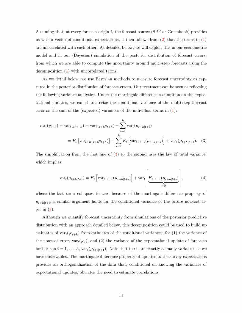
As we detail below, we use Bayesian methods to measure forecast uncertainty as cap-

tured in the posterior distribution of forecast errors. Our treatment can be seen as reflecting

the following variance analytics. Under the martingale difference assumption on the expec-

tational updates, we can characterize the conditional variance of the multi-step forecast

error as the sum of the (expected) variances of the individual terms in (1):

vart(yt+h) = vart( et t+h) = vart( et+h t+h) +

h∑i=1

vart(µt+h|t+i)

= Et

[vart+h( et+h t+h)

]+

h∑i=2

Et

[vart+i−1(µt+h|t+i)

]+ vart(µt+h|t+1). (3)

The simplification from the first line of (3) to the second uses the law of total variance,

which implies:

vart(µt+h|t+i) = Et

[vart+i−1(µt+h|t+i)

]+ vart

Et+i−1(µt+h|t+i)︸ ︷︷ ︸=0

, (4)

where the last term collapses to zero because of the martingale difference property of

µt+h|t+i; a similar argument holds for the conditional variance of the future nowcast er-

ror in (3).

Although we quantify forecast uncertainty from simulations of the posterior predictive

distribution with an approach detailed below, this decomposition could be used to build up

estimates of vart( et t+h) from estimates of the conditional variances, for (1) the variance of

the nowcast error, vart( et t), and (2) the variance of the expectational update of forecasts

for horizon i = 1, . . . , h, vart(µt+i|t+1). Note that these are exactly as many variances as we

have observables. The martingale difference property of updates to the survey expectations

provides an orthogonalization of the data that, conditional on knowing the variances of

expectational updates, obviates the need to estimate correlations.

11

3.2.2 Model of time-varying volatility

Based on the decomposition (1) and the martingale difference assumption (2), we specify

a multivariate stochastic volatility model for the available nowcast error and expectational

updates. As noted above, the forecast origin (denoted t) is roughly the middle of quarter

t, corresponding to the publication of the survey forecast. At the time the forecasters

construct their projections, they have data on quarter t− 1 and some macroeconomic data

on quarter t. We construct a data vector strictly contained in that information set and

define the data vector to contain H + 1 elements: the nowcast error for quarter t − 1 and

the revisions in forecasts for outcomes in quarters t through t+H − 1. (Although at origin

t the forecasts go through period t + H, the available forecast revisions only go through

period t + H − 1.) In the case of the SPF, which publishes forecasts for the current and

next four quarters, corresponding to H = 4 in our notation, we have the nowcast error and

four forecast updates to use. For comparability, our analysis of Greenbook forecasts relies

on the same choice of horizons.16

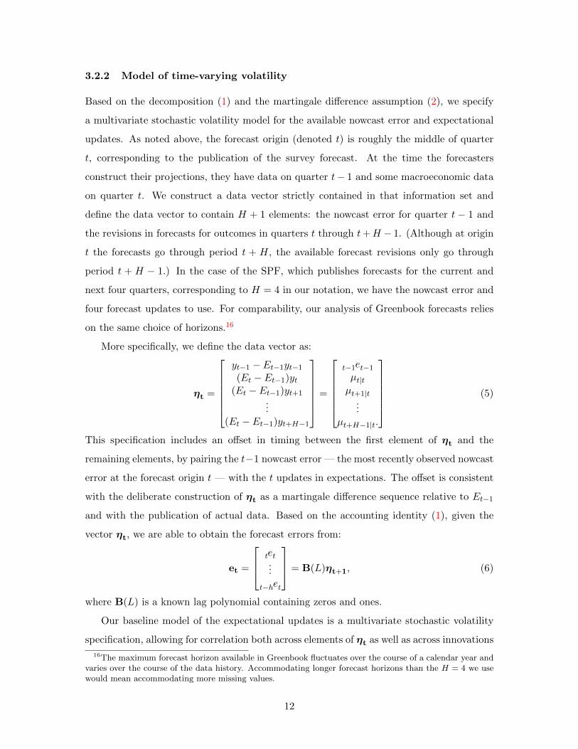
More specifically, we define the data vector as:

ηt =

yt−1 − Et−1yt−1(Et − Et−1)yt

(Et − Et−1)yt+1...

(Et − Et−1)yt+H−1

=

et−1 t−1µt|tµt+1|t

...µt+H−1|t.

(5)

This specification includes an offset in timing between the first element of ηt and the

remaining elements, by pairing the t−1 nowcast error — the most recently observed nowcast

error at the forecast origin t — with the t updates in expectations. The offset is consistent

with the deliberate construction of ηt as a martingale difference sequence relative to Et−1

and with the publication of actual data. Based on the accounting identity (1), given the

vector ηt, we are able to obtain the forecast errors from:

et =

et t...et−h t

= B(L)ηt+1, (6)

where B(L) is a known lag polynomial containing zeros and ones.

Our baseline model of the expectational updates is a multivariate stochastic volatility

specification, allowing for correlation both across elements of ηt as well as across innovations

16The maximum forecast horizon available in Greenbook fluctuates over the course of a calendar year andvaries over the course of the data history. Accommodating longer forecast horizons than the H = 4 we usewould mean accommodating more missing values.

12

to the log volatilities of each component of ηt. In other words we allow for correlation

between both level and scale shocks to η:

ηt = Aη̃t A =

1 0 0 . . . 0a21 1 0 . . . 0...

. . ....

aH+1,1 aH+1,2 . . . 1

(7)

η̃t = Λt0.5εt, εt ∼ i.i.d. N(0, IH+1), Λt ≡ diag(λ1,t, . . . , λH+1,t)

log(λi,t) = log(λi,t−1) + νi,t, i = 1, . . . ,H + 1

νt ≡ (ν1,t, ν2,t, . . . , νH+1,t)′ ∼ i.i.d. N(0,Φ).

where A, a lower triangular matrix with values of 1 on the diagonal, serves to capture cor-

relations across the components of ηt while correlations across the innovations to stochastic

volatility are captured by Φ. The variance-covariance matrix of ηt is given by Σt = AΛtA′.

While measures of correlation between elements of η do not enter directly in the vari-

ance calculus laid out above, the inclusion of non-zero lower-triangular coefficients in A

matters, at least somewhat, for our estimates, since we need to resort to full-information,

Bayesian sampling methods to estimate the time-varying volatilities as explained further

below. Moreover, some non-zero correlation between elements of ηt should generally be

expected, as persistence in the underlying macroeconomic variables forecasted by the SPF

should lead survey respondents to jointly revise updates in expectations of a given variable

at different horizons. In fact, if SPF forecasts were generated from the simple, univariate

AR-SV specification described above, expectational updates contained in ηt would be per-

fectly correlated with each other. For similar reasons, we allow innovations to log volatilities

to be correlated across the components of ηt, following the multivariate volatility specifica-

tion of studies such as Primiceri (2005). We obtained similar results for a model treating

the volatility innovations as mutually independent (as in, e.g., Cogley and Sargent 2005).

As this specification suggests, our focus in this paper is on a model of time-varying

volatility. For that purpose, we build the model around forecast errors and expectational

updates that are assumed mean zero.17 Reifschneider and Tulip (2017) also assume future

forecasts to be unbiased, treating any past historical bias as transitory.

By choosing an otherwise conventional, conditionally linear and Gaussian data-generating

process, our approach will yield prediction intervals and densities that are symmetric. In

17In preliminary analysis, we obtained similar results when, before estimating the model, we demeanedthe elements of the data vector ηt using a quasi-real time approach to computing a time-varying mean, withone-sided exponential smoothing.

13

doing so, we follow the broader literature (see references above) on including stochastic

volatility in time series models for macroeconomic forecasting. The last subsection of the

results section discusses possible extensions to accommodate asymmetries.

Although the baseline model features symmetry, the observed forecast errors and ex-

pectational updates need not be Gaussian. The model makes use of conditional innovations

(in εt) that are Gaussian, but this does not imply the observed forecast errors and expec-

tational updates to be Gaussian. In fact, the model implies that the distributions of the

observed expectational updates and forecast errors feature fat tails. We discuss below a

model extension to treat the conditional innovations εt as having fat tails.

3.2.3 Generalized model without MDS assumption

As noted above, our baseline specification reflects an assumption that the vector of expec-

tational updates forms a martingale difference sequence, consistent with full rationality of

the forecasts. This assumption helps to yield a parsimonious model, and parsimony is well

known to be helpful in forecasting. However, studies such as Croushore (2010) and Reif-

schneider and Tulip (2017) provide evidence of some biases in forecasts from sources such

as SPF and Greenbook. Moreover, recent research by Coibion and Gorodnichenko (2015)

and Mertens and Nason (2015), among others, has shown survey-based forecasts to display

information rigidities, reflected in some serial correlation in forecast errors.

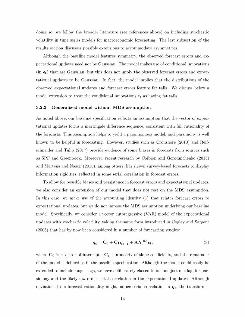
To allow for possible biases and persistence in forecast errors and expectational updates,

we also consider an extension of our model that does not rest on the MDS assumption.

In this case, we make use of the accounting identity (1) that relates forecast errors to

expectational updates, but we do not impose the MDS assumption underlying our baseline

model. Specifically, we consider a vector autoregressive (VAR) model of the expectational

updates with stochastic volatility, taking the same form introduced in Cogley and Sargent

(2005) that has by now been considered in a number of forecasting studies:

ηt = C0 + C1ηt−1 + AΛt0.5εt, (8)

where C0 is a vector of intercepts, C1 is a matrix of slope coefficients, and the remainder

of the model is defined as in the baseline specification. Although the model could easily be

extended to include longer lags, we have deliberately chosen to include just one lag, for par-

simony and the likely low-order serial correlation in the expectational updates. Although

deviations from forecast rationality might induce serial correlation in ηt, the transforma-

14

tion from forecast errors to forecast updates still serves as a pre-whitening step, given that

deviations from rationality in survey forecasts appear limited. As a simple check of the

serial correlation in the expectational updates, for each variable we estimated vector au-

toregressions based on the vector ηt using 0 to 4 lags and assessed fit with the BIC. The

BIC indicates the optimal lag order to be 0 for the unemployment rate and CPI inflation

and 1 for GDP growth, GDP inflation, and the T-bill rate. Our use of a (Bayesian) VAR

with one lag appears consistent with this simple check.

As detailed below, we estimate this extended model — referred to below as the VAR-

SV specification — with conventional Minnesota-type priors on C0 and C1.18 This model

allows for non-zero means and serial correlation of the expectational updates. We obtain

the forecast errors using the accounting identity et = B(L)ηt+1, where B(L) is a known

lag polynomial containing zeros and ones.

3.2.4 Estimating the model and forecast uncertainty

The baseline model of (7) and the extension (8) can be estimated by Bayesian Markov

chain Monte Carlo methods (a Gibbs sampler). We focus on describing the estimation of

the baseline specification; the estimation of the VAR model involves adding a conventional

Gibbs step to draw the VAR coefficients from their conditional posterior (see, e.g., Clark and

Ravazzolo 2015). The baseline model’s algorithm involves iterating over the following three

blocks: First, taking estimates of Λt0.5 as given, we employ recursive Bayesian regressions

with diffuse priors to estimate the lower triangular coefficients of A, which is tantamount

to a Choleski decomposition of η into η̃.19 Second, we estimate the stochastic volatilities

of η̃t using the multivariate version of the Kim, Shephard, and Chib (1998) [henceforth,

KSC] algorithm introduced into macroeconomics by Primiceri (2005). Third, given draws

for the sequences of log (λi,t) for all i and t we estimate the variance-covariance matrix

of innovations to the SV processes, Φ, using an inverse Wishart conjugate-prior centered

around a mean equal to a diagonal matrix with 0.22 on its diagonal using 9 + H degrees

of freedom, which makes the prior slightly informative. Note that our setting of the prior

mean is in line with settings used in some studies of stochastic volatility, including Stock

and Watson (2007) and Clark (2011).

18For the VAR’s coefficients, the prior means are all zero, and the standard deviations take the Minnesotaform, with the hyperparameter governing overall shrinkage set at 0.2, the hyperparameter for “other” lagsrelative to “own” lags set at 0.5, and the hyperparameter governing intercept shrinkage set at 1.

19To initialize the Gibbs sampler, we draw initial values for each lower-triangular coefficients of A fromindependent standard normal distributions.

15

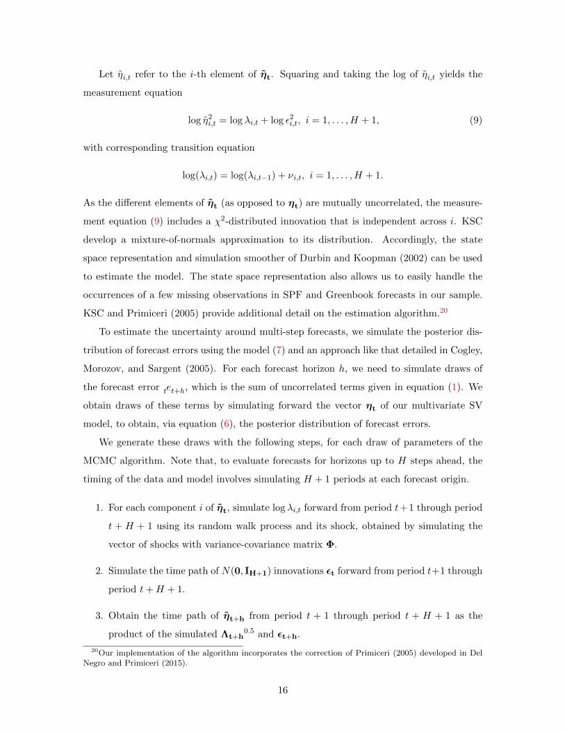
Let η̃i,t refer to the i-th element of η̃t. Squaring and taking the log of η̃i,t yields the

measurement equation

log η̃2i,t = log λi,t + log ε2i,t, i = 1, . . . ,H + 1, (9)

with corresponding transition equation

log(λi,t) = log(λi,t−1) + νi,t, i = 1, . . . ,H + 1.

As the different elements of η̃t (as opposed to ηt) are mutually uncorrelated, the measure-

ment equation (9) includes a χ2-distributed innovation that is independent across i. KSC

develop a mixture-of-normals approximation to its distribution. Accordingly, the state

space representation and simulation smoother of Durbin and Koopman (2002) can be used

to estimate the model. The state space representation also allows us to easily handle the

occurrences of a few missing observations in SPF and Greenbook forecasts in our sample.

KSC and Primiceri (2005) provide additional detail on the estimation algorithm.20

To estimate the uncertainty around multi-step forecasts, we simulate the posterior dis-

tribution of forecast errors using the model (7) and an approach like that detailed in Cogley,

Morozov, and Sargent (2005). For each forecast horizon h, we need to simulate draws of

the forecast error et t+h, which is the sum of uncorrelated terms given in equation (1). We

obtain draws of these terms by simulating forward the vector ηt of our multivariate SV

model, to obtain, via equation (6), the posterior distribution of forecast errors.

We generate these draws with the following steps, for each draw of parameters of the

MCMC algorithm. Note that, to evaluate forecasts for horizons up to H steps ahead, the

timing of the data and model involves simulating H + 1 periods at each forecast origin.

1. For each component i of η̃t, simulate log λi,t forward from period t+1 through period

t + H + 1 using its random walk process and its shock, obtained by simulating the

vector of shocks with variance-covariance matrix Φ.

2. Simulate the time path of N(0, IH+1) innovations εt forward from period t+1 through

period t+H + 1.

3. Obtain the time path of η̃t+h from period t + 1 through period t + H + 1 as the

product of the simulated Λt+h0.5 and εt+h.

20Our implementation of the algorithm incorporates the correction of Primiceri (2005) developed in DelNegro and Primiceri (2015).

16

4. Transform η̃t into ηt by multiplication with A.

5. At each horizon h, construct the draw of the forecast error by summing the relevant

terms from the previous step according to the decomposition (1). Construct the draw

of the forecast by adding the forecast error to the corresponding point forecast from

SPF.

Given the set of draws produced by this algorithm, we compute the forecast statistics

of interest. For example, we compute the standard deviation of the forecast errors and the

percentage of observations falling within a plus/minus one standard-error band. In the next

section, we detail these and the other forecast evaluation metrics considered.

3.2.5 An alternative approach assuming constant variances of forecast errors

In light of common central bank practice (e.g., Reifschneider and Tulip 2007, 2017 and

the fan charts in the Federal Reserve’s SEP), the most natural benchmark against which

to compare our proposed model-based approach is one based on historical forecast error

variances treated as constant over some window of time and into the future. That is, at

each forecast origin t, prediction intervals and forecast densities can be computed assuming

normally distributed forecast errors with variance equal to the variance of historical forecast

errors over the most recent R periods (e.g., the SEP fan charts are based on forecast errors

collected over the previous 20 calendar years).21 Accordingly, we report results obtained

under a similar approach, where we will collect continuously updated estimates generated

from rolling windows of forecast errors covering the most recent R = 60 quarterly obser-

vations. For simplicity, below we will refer to this specification as the “constant variance”

approach and denote it with “FE-CONST,” even though it acknowledges the potential for

variance changes over time by using a rolling window of observations.22 Note, too, that this

benchmark approach differs from our model-based approach in that the benchmark uses

forecast errors directly, whereas our model-based approach uses the expectational updates

and obtains forecast errors as linear combinations of the expectational updates. In addi-

tion, the FE-CONST approach differs in that it relies merely on sample moments without

21A number of other studies, such as Kenny, Kostka, and Masera (2014) and Rossi and Sekhposyan (2014),have also used normal distributions based on a given point forecast and error variance.

22We obtained very similar results with a more parametric approach or model assuming a time-invariantnormal distribution for the nowcast error and the expectational updates collected in ηt (while maintainingthe martingale difference sequence assumption): ηt ∼ N(0,Σ). We employ Bayesian methods to estimatethis model within the quasi-real-time setup described above, assuming a diffuse inverse-Wishart prior.

17

specifying an explicit probability model for the data.

Of course, a key choice is the size of the rolling window (R) used in the constant variance

approach. As noted above, some central banks use windows of 40 or 80 quarterly observa-

tions; Clements (2016) uses 50 quarterly observations. In our analysis, there is an important

sample tradeoff in data availability: making the rolling window bigger shortens the forecast

sample available for evaluation. Accordingly, in our baseline results, we essentially split the

difference, so to speak, and use a rolling window of 60 observations in the constant variance

benchmark. With this setting, we have available the following samples for the evaluation

of SPF forecasts: 1984:Q1–2017:Q1 for GDP growth, unemployment, and GDP inflation;

and 1996:Q4–2017:Q1 for CPI inflation and the T-bill rate. While the sample of available

Greenbook forecasts permits similar start dates, the end date for evaluating is 2011:Q4, re-

flecting the five-year blackout period for publication. As we detail in the robustness results

below, our main findings apply to rolling windows shorter or longer than the baseline.

4 Evaluation metrics

The previous section described two alternative volatility models — our proposed stochastic

volatility model, our extension to a VAR with stochastic volatility, and a constant-variance

benchmark. This section considers two measures of density forecast accuracy to assess the

absolute and relative performance of these models. The first measure focuses on the ac-

curacy of prediction intervals. In light of central bank interest in uncertainty surrounding

forecasts, confidence intervals, and fan charts, a natural starting point for forecast density

evaluation is interval forecasts — that is, coverage rates. Recent studies such as Giordani

and Villani (2010) and Clark (2011) have used interval forecasts as a measure of the cali-

bration of macroeconomic density forecasts. Accordingly, we will report the frequency with

which real-time outcomes for growth, unemployment, inflation, and the Treasury bill rate

fall inside one-standard deviation prediction intervals. We compare these coverage rates to

the nominal coverage rate implied by the percentiles of the normal distribution for the area

between plus/minus a one standard-deviation error; up to rounding this covers 68 percent.23

A frequency of more (less) than 68 percent means that, on average over a given sample, the

estimated forecast density is too wide (narrow). We judge the significance of the results

23We also considered analyzing results for the 90 percent prediction interval. However, with more obser-vations available at the 68 percent level than the 90 percent level, we chose to devote attention to the formerrather than the latter.

18

using p-values of t-statistics for the null hypothesis that the empirical coverage rate equals

the nominal rate of 68 percent; we compute the t-statistics with the HAC-robust variance

estimate of Newey and West (1987) and a lag order equal to the forecast horizon plus 2.

Our second measure of density accuracy is the continuous ranked probability score

(CRPS). As indicated in Gneiting and Raftery (2007) and Gneiting and Ranjan (2011),

some researchers view the CRPS as having advantages over the log score.24 In particular,

the CRPS does a better job of rewarding values from the predictive density that are close

to but not equal to the outcome, and it is less sensitive to outlier outcomes. The CRPS,

defined such that a lower number is a better score, is given by

CRPSt(yot+h) =

∫ ∞−∞

(F (z)− 1{yot+h ≤ z}

)2dz = Ef |Yt+h − yot+h| − 0.5Ef |Yt+h − Y ′t+h|,

(10)

where F denotes the cumulative distribution function associated with the predictive density

f , 1{yot+h ≤ z} denotes an indicator function taking value 1 if the outcome yot+h ≤ z and 0

otherwise, and Yt+h and Y ′t+h are independent random draws from the posterior predictive

density. We compute the CRPS using the empirical CDF-based approximation given in

equation (10) of Krueger, et al. (2017). We gauge the significance of differences in CRPS on

the basis of p-values of t-statistics for equality of average CRPS, using HAC-robust variances

computed with the Newey and West (1987) estimator and a lag order equal to the forecast

horizon plus 2.

As noted above, a number of studies have compared the density forecast performance

of time series models with stochastic volatility against time series models with constant

variances (e.g., Clark 2011, Clark and Ravazzolo 2015, D’Agostino, Gambetti, and Giannone

2013, and Diebold, Schorfheide, and Shin 2016). In some cases, the models with constant

variances are estimated with rolling windows of data. In some respects, the comparisons

in this paper are similar to these studies. However, a key difference is that we take the

point forecasts as given from a source such as the SPF, whereas, in these papers, the point

forecasts vary with each model. So, for example, in Clark’s (2011) comparison of a BVAR

with stochastic volatility against a BVAR with constant variances estimated over a rolling

window of data, the use of a rolling window affects the point forecasts. As a result, the

evidence on density forecast accuracy from the VAR and DSGE literature commingles effects

of conditional means and variances with rolling windows versus other estimators and other

24Recent applications can be found, for example, in Ravazzolo and Vahey (2014) and Clark and Ravazzolo(2015).

19

models. In contrast, in this paper, by using point forecasts from SPF or Greenbook, we are

isolating influences on density accuracy due to variances.

5 Results

We begin this section of results with a brief review of the data properties and with full-

sample estimates of stochastic volatility. We then provide the out-of-sample forecast results,

first on coverage and then on density accuracy as measured with the CRPS. The next

subsection provides a summary of various robustness checks, including results for Greenbook

forecasts. The section concludes with a discussion of directions in which the model could

be extended.

5.1 Full-sample

As noted above, the data used to estimate our model are the expectational updates (for

simplicity, defined broadly here to include the nowcast error) contained in ηt. Figures 1

and 2 report these data for GDP growth and the unemployment rate, respectively; the data

for the other variables, along with the forecast errors, are provided in the supplementary

appendix, in the interest of brevity. Qualitatively, the results we highlight for GDP growth

and unemployment also apply to the other variables.

As implied by the forecast error decomposition underlying our model, the expectational

updates are fairly noisy. Although there is some small to modest serial correlation in the

data on the longer-horizon expectational updates, this serial correlation is much smaller

than that in the multi-step forecast errors. As an example, for the unemployment rate,

compare the 4-step ahead expectational update in Figure 2 to the 4-step ahead forecast

errors in the Supplementary Appendix’s Figure 5.

Another notable feature of the data is that, at longer forecast horizons, the expectational

updates are smaller in absolute size than are the corresponding forecast errors. This feature

is more or less inherent to expectational updates. In addition, in most cases (less clearly so

for the unemployment rate than the other variables), the absolute sizes of the expectational

updates appear to be larger in the period before the mid-1980s than afterward, consistent

with the Great Moderation widely documented in other studies. For growth, unemployment,

and the T-bill rate, the expectational errors tend to be larger (in absolute value) in recessions

than expansions.

20

Figures 3 to 7 provide the time-varying volatility estimates obtained with the expecta-

tional updates. Specifically, the red lines in each figure provide the full-sample (smoothed)

estimates of stochastic volatility (reported as standard deviations, or λ0.5i,t in the model

notation). For comparison, the figures include (in gray bars) the absolute values of the

expectational updates, which roughly correspond to the objects that drive the model’s

volatility estimates, as well as quasi-real time estimates of stochastic volatility (black lines).

The quasi-real time estimates are obtained by looping over time and estimating an historical

volatility path at each forecast origin; these estimates underlay the forecast results consid-

ered in the next section. Note that, to improve chart readability by limiting the number

of panels on each page to four, we omit from each chart the estimates for the 3-step ahead

forecast horizon; these unreported estimates are consistent with the results summarized

below.

Across variables, the volatility estimates display several broad features, as follows.

• The time variation in volatility is considerable. The highs in the volatility estimates

are typically 3 to 4 times the levels of the lows in the estimates.

• Some of the time variation occurs at low frequencies, chiefly with the Great Mod-

eration of the 1980s. The Great Moderation is most evident for GDP growth, the

unemployment rate (less so for the nowcast horizon than longer horizons), and infla-

tion in the GDP price index. For CPI inflation, the volatility estimate declines even

though the available sample cuts off most of the period preceding the typical dating

of the Great Moderation. For the T-bill rate, for which the sample is shorter, as with

the CPI, the SV estimate shows a sharp falloff at the beginning of the sample; this

falloff is consistent with SV estimates from time series models obtained with longer

samples of data (e.g., Clark and Ravazzolo 2015).

• Some of the time variation is cyclical, as volatility has some tendency to rise temporar-

ily around recessions. For example, the volatility of GDP growth and unemployment

rises with most recessions, and the volatility of the T-bill rate picks up around the 2001

and 2007-2009 recessions. The cyclical pattern appears smaller for inflation, except

that CPI inflation spiked sharply around the time of the Great Recession, presumably

due to the dramatic, unexpected falloff in inflation that occurred as commodity prices

collapsed.

21

• The overall magnitude of volatility for the nowcast horizon versus the expectational

updates for longer horizons varies by variable, probably reflecting data timing. For

growth and both measures of inflation, the level of volatility at the nowcast horizon

exceeds the level of volatility at longer horizons. However, for the unemployment

rate and T-bill rate, nowcast volatility is lower than longer-horizon update volatility,

probably because the nowcast is often or always formed with the benefit of one month

of data (for the unemployment rate and T-bill rate) on the quarter.

• For the most part, for the period since the 1980s, the contours of SV estimates for

inflation in the GDP price index and CPI are similar. There are of course some

differences, including the relatively sharp late-2000’s rise for the CPI that probably

reflects a bigger influence of commodity prices on CPI inflation than GDP inflation and

a larger rise in CPI volatility in 1991 that may reflect a shorter sample for estimation

than is available with the GDP price index.

• As expected, the full sample (smoothed) SV estimates are modestly smoother than

the quasi-real time (QRT) estimates. One dimension of this smoothness is that the

QRT estimates tend to respond to recessions with a little delay; around recessions,

the full sample estimates rise sooner than do the QRT estimates. In addition, in the

case of CPI inflation, the late 2000’s rise in volatility is larger in quasi-real time than

in the full sample estimates.

5.2 Out-of-Sample Forecasts

As noted above, to assess forecast accuracy, we consider both interval forecasts and density

accuracy as measured by the CRPS. We begin with the interval forecasts. Figures 8-12

report the forecast errors for each variable along with one-standard deviation intervals, one

set (in blue) obtained with the constant variance approach applied to a 60 observation rolling

window of forecast errors and the other (in red) obtained from our stochastic volatility model

of ηt. (We focus on forecast errors for simplicity; instead reporting the point forecasts and

confidence bands around the forecasts would yield the same findings.) Again, for readability,

we omit from the charts the estimates for the 3-step ahead horizon. Figures 8-12 provide

a read on time variation in the width of confidence intervals and the accuracy of the two

approaches. Table 1 quantifies empirical coverage rates. In the discussion below, we focus

on one-standard deviation (treated as 68 percent, as noted above) coverage rates, because

22

there are far fewer observations available for evaluating accuracy further out in the tails of

the distributions.

The charts of the time paths of one-standard deviation confidence intervals display the

following broad patterns.

• Both types of estimates (constant variances with rolling windows and our SV-based

estimates) display considerable time variation in the width of the intervals. For GDP

growth, unemployment, and GDP inflation (for which the evaluation sample dates

back to 1984), the width of the constant variance estimates progressively narrows over

the first half of the sample, reflecting the increasing influence of the Great Moderation

on the rolling window variance estimates. In contrast, for CPI inflation, for which the

sample is also shorter, the constant variance bands tend to widen as the sample moves

forward.

• Consistent with the SV estimates discussed above, the width of the confidence bands

based on our SV model-based approach varies more than does the width of intervals

based on constant variances. For GDP growth, unemployment, and GDP inflation,

the SV model-based intervals narrow sharply in the first part of the sample (more so

than the constant variance estimates) and then widen significantly (again, more so

than the constant variance estimates) with the Crisis and, in the case of GDP growth

and the T-bill rate, the recession of 2001. For most of the sample, the interval widths

are narrower with the SV approach than the constant variance approach; however,

this pattern does not so generally apply to CPI inflation.

• Across horizons, the contours of the confidence intervals (for a given approach) are

very similar. With the SV model-based estimates, the similarities across horizons

are particularly strong for horizons 1 through 4 (omitting the nowcast horizon).25

Although the intervals display some differences in scales, they move together across

horizons. In the model estimates, this comovement is reflected in estimates of the

volatility innovation variance matrix Φ, which allows and captures some strong cor-

relation in volatility innovations across horizons.26 More broadly, with these variance

25Note that, for the unemployment and T-bill rates, the interval widths for the nowcast are narrowerthan those at longer horizons probably due to data timing, with forecasters often (unemployment) or always(T-bill rate) having available one month of data on the quarter.

26In unreported results, we have used the estimates of Φ at each forecast origin to construct the correlationmatrix of the innovations to the volatility processes of the model. These estimates are fairly stable over

23

estimates reflecting forecast uncertainty, as uncertainty varies over time, that uncer-

tainty likely affects all forecast horizons, in a way captured by these SV estimates.

The coverage rates reported in Table 1 for SPF forecasts quantify the accuracy of the

one-standard deviation intervals shown in Figures 8-12. These show the intervals based on

our stochastic volatility model to be consistently more accurate than the intervals based on

the constant variance approach applied to forecast errors. Although we cannot claim that

the SV-based approach yields correct coverage in all cases, it does so in the large majority

of cases; the gap between the empirical and nominal rate is significant only in the case of

TBILL forecasts at short horizons. Moreover, the SV-based approach typically improves

on the alternative approach, which in most cases yields coverage rates above 68 percent,

reflecting bands that are too wide. For example, for GDP growth, the SV-based coverage

rates range (across horizons) from 69.5 percent to 72.9 percent, with no departures from

68 percent large enough to be statistically significant, whereas the constant variance-based

rates range from 76.5 percent to 79.7 percent, with all five departures from 68 percent large

enough to be statistically significant. For the T-bill rate, the SV-based rates are much

lower than the constant-variance-based rates at forecast horizons of 2 quarters or more —

e.g., at the 2-step horizon, 72.84 percent with SV versus 83.95 percent for the constant

variance baseline. For the inflation measures considered, results for the GDP price index

are comparable to those for real GDP. But for CPI inflation, the coverage rates obtained

with our SV model are similar to those obtained with the constant variance benchmark

approach.

To provide a broader assessment of density forecast accuracy, Table 2 reports the average

CRPS. To simplify comparison, the table reports the level of the CRPS obtained with the

constant variance approach and the percentage improvement in the CRPS of the SV-based

forecasts relative to the constant variance-based forecasts. With SPF forecasts, for all

variables, our SV model consistently offers density accuracy gains over the constant variance

specification. The gains are largest for the T-bill rate, ranging from 5 to 12 percent. For

GDP growth, the gains are still healthy, ranging from 3 to 9 percent. The gains in CRPS

accuracy over the benchmark are statistically significant for growth and the T-bill rate.

For the unemployment rate and the inflation measures, the gains are smaller (and only

occasionally significant), but consistently positive, ranging from 0.9 to 3.3 percent. As

time, with a largest eigenvalue between 2 and 3 (depending on the variable), the second largest eigenvalueequal to about 1, and the remaining eigenvalues progressively smaller, but none close to 0.

24

noted above, although some studies have found modestly larger density gains associated

with SV, these studies typically commingle benefits to point forecasts with benefits to the

variance aspect of the density forecasts. In our case, the point forecasts are the same across

the approaches, so any gains in density accuracy come entirely from variance-related aspects

of the forecast distribution.

5.2.1 Robustness to Rolling Window Choice

We have also examined the performance of SV against the constant variance approach with

the rolling window underlying the constant variance specification either shorter or longer

than the 60 observation setting of our baseline results. One alternative is to lengthen

the rolling window to 80 observations, in line with the roughly 20 year sample underlying

the historical forecast RMSEs reported in the Federal Reserve’s SEP (Table 2).27 Note,

however, that with this setting, the comparison to the baseline isn’t entirely a clean one,

because the longer rolling window shortens (pulling the start point forward) the forecast

evaluation sample by 20 observations.

Lengthening the rolling window underlying the benchmark constant variance approach

does not alter the picture we painted above: the constant variance approach commonly

yields coverage rates in excess of the nominal rate of 68 percent (see Appendix Table 1).

In many cases, the coverage rates are higher with the 80 observation window than the 60

observation window. With the exception of CPI inflation, the empirical coverage rates for

SPF forecasts are almost all significantly above 68 percent. Lengthening the rolling window

underlying the benchmark constant variance approach does not alter the broader picture

of density forecast accuracy characterized above for the CRPS. It remains the case that

our SV specification offers consistent gains to CRPS accuracy over the constant variance

approach.

The other alternative we consider shortens the rolling window to 40 observations. With

this window setting, we could lengthen the evaluation sample, but to facilitate comparisons

to the baseline case, we leave the evaluation sample unchanged from the baseline. In the

estimates, shortening the rolling window to 40 observations does not materially change the

picture provided by the baseline results, although in forecast coverage, it slightly reduces

the advantage of our SV-based model. As detailed in the appendix (Appendix Table 3),

coverage rates fall some for GDP growth and GDP inflation, making rates for the constant

27For details, see http://www.federalreserve.gov/foia/files/20140409-historical-forecast-errors.pdf.

25

variance benchmark broadly comparable to those for the SV model. However, even with the

shorter observation window for the constant variance approach, the SV model yields better

coverage for the unemployment and T-bill rates. Density accuracy as measured by the

CRPS is only modestly affected (see Appendix Table 4) by shortening the rolling window

from 60 to 40 observations, such that our SV model-based approach maintains the same

consistent advantage described above.

5.2.2 Out-of-Sample Results for VAR-SV specification

In the interest of brevity, in examining the efficacy of extending our baseline SV model to the

VAR-SV specification, we present the out-of-sample results and omit figures with the full-

sample VAR-SV estimates of volatility. The full-sample estimates for the VAR-SV model

are qualitatively similar to the baseline SV estimates. Tables 3 and 4 provide one-standard

deviation coverage rates and CRPS values for the VAR-SV model, with comparison to the

baseline constant forecast error variance approach (repeating these results from Tables 1

and 2 for convenience).

The coverage rates reported in Table 3 for SPF forecasts show the intervals based on

the VAR-SV model to be modestly more accurate than the intervals based on the constant

variance approach applied to forecast errors (for convenience, Table 3 contains benchmark

coverage rates also provided in Table 1). In broad terms, the advantages of the VAR-SV

model over the benchmark constant variance case can be seen in the number of asterisks,

with fewer statistically significant departures from correct coverage. As examples, the VAR-

SV model yields coverage rates much lower than the constant variance benchmark for the

unemployment and T-bill rates. However, in most cases, the advantages of the VAR-SV

model are smaller than those of the baseline SV model. In most cases, coverage rates are

higher with the VAR-SV model than the baseline SV model. This is associated with less

accurate coverage in most cases, except for the T-bill rate.

For broader density forecast accuracy, the CRPS averages provided in Table 4 for SPF

forecasts show the VAR-SV specification to be useful for some variables and not others.

For GDP growth, the unemployment rate, and the T-bill rate, the VAR-SV model yields

density forecasts more accurate than those obtained with the benchmark constant vari-

ance approach, with gains up to 6 percent for growth, up to 9 percent for unemployment,

and up to 23 percent for the T-bill rate. For the inflation variables, the VAR-SV model

yields density forecasts modestly less accurate than the benchmark. When compared to the

26

baseline SV model, the extension provided by the VAR-SV model is somewhat helpful for

unemployment and T-bill forecasts (boosting the CRPS noticeably) and somewhat harmful

for the other variables.

On balance, this evidence suggests that extending our baseline SV model to depart

from its MDS assumption has a mixed payoff. It helps along some, but not all, dimensions.

This finding suggests that the pre-whitening of multi-step forecast errors provided by the

accounting identity used to obtain our baseline model is largely sufficient, although there

are some variables for which adding VAR dynamics is a useful supplement to the baseline

pre-whitening.

5.2.3 Out-of-Sample Results for Greenbook

In the interest of brevity, in examining the robustness of our results to the use of Greenbook

rather than SPF forecasts, we present the out-of-sample results and omit figures with the

full-sample ηt and SV estimates. The full-sample estimates with Greenbook are qualita-

tively similar to those for SPF.

Figures 13-16 report the Greenbook forecast errors for each variable along with one-

standard deviation intervals, one set (in blue) obtained with the constant variance approach

applied to forecast errors and a 60 observation rolling window of observations and the

other (in red) obtained from our stochastic volatility model. The lower portion of Table 1

quantifies empirical coverage rates of one-standard deviation intervals, taking the nominal

rate to be 68 percent.

In broad terms, along most dimensions, the pattern of interval forecast results for Green-

book are similar to those for SPF (in reviewing the charts, recall that the Greenbook sample

ends almost six years earlier). First, as in the SPF results, both types of volatility estimates

(constant variances with rolling windows and our SV-based estimates) display considerable

time variation in the width of the intervals. However, in this dimension, the Greenbook

results appear somewhat different in that, up to the mid-2000s, the bands around CPI in-

flation are fairly stable in width, whereas the SPF-based bands become gradually wider.

Second, the width of the confidence bands based on our SV approach varies more than

does the width of intervals based on constant variances. For example, for most variables,

the bands widen substantially with the Great Recession and with earlier recessions. Third,

across horizons, the contours of the confidence intervals (for a given approach) are very

similar.

27

The coverage rates for Greenbook forecasts reported in Table 1 quantify the accuracy

of the one-standard deviation intervals shown in Figures 13-16. On balance, the intervals

based on our stochastic volatility model perform comparably to those based on the constant

variance approach. For CPI inflation, coverage rates are moderately better with stochastic

volatility than in the benchmark. For the unemployment rate, coverage rates also tend

to be somewhat closer to the nominal size with the stochastic volatility model than the

constant variance approach. But for GDP growth and inflation, coverage rates are quite

similar across the two approaches.

The CRPS averages for Greenbook forecasts given in the lower part of Table 2 show

that, in most cases, our SV model consistently offers some density accuracy gains over

the constant variance specification. In broad terms, the gains are comparable to those

observed with SPF forecasts, but a little smaller in most cases. For example, for GDP

growth, the gains range from about 3 to 9 percent with SPF forecasts and 2 to 6 percent

with Greenbook forecasts. For the extension to the VAR-SV models, the patterns in the

Greenbook forecasts are similar to those described above for the SPF forecasts. In 68

percent coverage, extending the SV model to include VAR dynamics does not seem to help

much. But in broader density accuracy as captured by the CRPS, the extension to include

VAR dynamics reduces accuracy for inflation variables but mostly preserves or extends the

gains from SV for GDP growth and unemployment.

On balance, our main results obtained with SPF forecasts are corroborated by estimates

with Greenbook forecasts, although perhaps the efficacy of stochastic volatility is modestly

less compelling with Greenbook than with SPF forecasts.

6 Model extensions

Along several dimensions, the model and data could be extended to include additional

features. In the interest of brevity, we don’t pursue these extensions, but we briefly describe

them, leaving them as subjects for future research.

First, the multivariate stochastic volatility model could be extended to allow fat tails in

the conditional errors εt, drawing on the specification of Jacquier, Polson, and Rossi (2004)

or an outlier-filtering approach of Stock and Watson (2016). Some macroeconomic studies

have used fat-tailed SV specifications with time series or structural models, with varying

success (e.g., Chiu, Mumtaz, Pinter 2015; Clark and Ravazzolo 2015; Curdia, Del Negro,

28

Greenwald 2015). Stock and Watson (2016) find a related, mixture of normals approach

to filtering inflation outliers to be helpful. We actually examined extending our model to

include the Stock-Watson mixture. In our setting with SPF forecasts, this model extension

helped to reduce the influence of some outliers on our stochastic volatility estimates but to

have little effect on our baseline forecast results.

Second, the model could be extended to make use of forecasts from multiple sources. In

Reifschneider and Tulip (2007, 2017) and the Federal Reserve’s SEP, forecast accuracy is es-

timated by averaging the root mean square errors of a range of forecasts. In our framework,

multiple forecasts could be exploited by treating each forecast source as a different mea-

surement on a common volatility process. That is, the data vector ηt could be expanded to

include multiple measurements of the nowcast error and each of the expectational updates,

driven by a common set of the H + 1 volatility processes and conditional errors.28

Third, the multivariate stochastic volatility model could be extended to include all of

the variables being forecast. We have proceeded on a variable-by-variable to keep the

computations tractable. However, it is likely possible — although more complicated — to

consider some variables jointly, with the model extended (as described above) to permit

correlation across the nowcast errors and expectational updates of different variables.

Finally, there are some ways our model might in future research be extended to allow

asymmetries in the forecast (error) distributions. As noted above, we have interpreted past

periods of non-zero forecast errors as biases and removed them, allowing some slow time

variation intended to be consistent with evidence in Croushore (2010), before estimation and

forecast evaluation. However, some might interpret these past periods of non-zero errors as

representing asymmetries in the forecast distribution that should be explicitly modeled. It

could be possible to draw on the finance literature on stochastic volatility with asymmetries

(see, e.g., Asai, McAleer, and Yu’s (2006) review of multivariate SV models with asymme-

tries) to extend our macroeconomic model to allow asymmetries. Some might also believe

it important to explicitly model asymmetries in variables such as the unemployment rate

and T-bill rate, particularly given effective lower bounds on these variables and historical

work such as Neftci (1984) and Montgomery, et al. (1998) on the evidence of asymmetries

in the unemployment rate.

28The model could further be extended by easing up on the common factor restrictions by, for example,introducing some measurement noise to each forecast source.

29

7 Conclusions

Motivated in part by central bank fan charts that use historical forecast errors to quantify

the uncertainty around forecasts, this paper develops a multiple-horizon specification of

stochastic volatility for forecast errors from sources such as SPF, Blue Chip, or the Fed’s

Greenbook, for the purpose of improving the accuracy of uncertainty estimates around

the forecasts. Our approach can be used to form confidence bands around forecasts that

allow for variation over time in the width of the confidence bands; the explicit modeling of

time variation of volatility eliminates the need for somewhat arbitrary judgments of sample

stability.

At each forecast origin, we have available the forecast error from the previous quarter

and forecasts for the current quarter and the subsequent four quarters. To address the

challenge of overlap in forecast errors across horizons, we formulate the model to make use

of the current quarter (period t) nowcast error and the forecast updates for subsequent

quarters (forecasts made in period t less forecasts made in period t−1). These observations

reflect the same information as the set of forecast errors for all horizons. However, unlike

the vector of forecast errors covering multi-step horizons, the vector containing the forecast

updates is serially uncorrelated, under conventional assumptions that the forecasts represent

a vector of conditional expectations. For this vector of observations, we specify a multiple-

horizon stochastic volatility model that can be estimated with Bayesian MCMC methods.

From the estimates, we are able to compute the time-varying conditional variance of forecast

errors at each horizon of interest.

Estimates of the model with the full sample of forecasts display considerable historical

variation in forecast error variances, at each forecast horizon. Consistent with evidence

from the VAR and DSGE literatures, the forecast error variances shrink significantly with

the Great Moderation and tend to rise — temporarily — with each recession, most sharply

for the most recent Great Recession. To assess the performance of our approach in out-of-

sample forecasting we assess forecast coverage rates and the accuracy of density forecasts

as measured by the continuous ranked probability score. We show that, by these measures,

our proposed approach yields forecasts more accurate than those obtained using sample

variances computed with rolling windows of forecast errors as in approaches such as Reif-

schneider and Tulip (2007, 2017).

30

References

Abel, Joshua, Robert Rich, Joseph Song, and Joseph Tracy (2016), “The Measurement andBehavior of Uncertainty: Evidence from the ECB Survey of Professional Forecasters,”Journal of Applied Econometrics 31, 533-550. https://doi.org/10.1002/jae.2430

Asai, Manabu, Michael McAleer, and Jun Yu (2006), “Multivariate Stochastic Volatility: AReview,” Econometric Reviews 25, 145-175. https://doi.org/10.1080/07474930600713564

Boero, Gianna, Jeremy Smith, and Kenneth F. Wallis (2015), “The Measurement and Char-acteristics of Professional Forecasters’ Uncertainty,” Journal of Applied Econometrics30, 1029-1046. https://doi.org/10.1002/jae.2400

Carriero, Andrea, Todd E. Clark, and Massimiliano Marcellino (2016), “Common DriftingVolatility in Large Bayesian VARs,” Journal of Business and Economic Statistics 34,375-390. https://doi.org/10.1080/07350015.2015.1040116

Chiu, Ching-Wai (Jeremy), Haroon Mumtaz, and Gabor Pinter (2015), “Forecasting withVAR models: Fat Tails and Stochastic Volatility,” Bank of England Working Paper No.528.

Clark, Todd E. (2011), “Real-time Density Forecasts from BVARs with Stochastic Volatil-ity,” Journal of Business and Economic Statistics 29, 327-341. https://doi.org/10.1198/jbes.2010.09248

Clark, Todd E. and Francesco Ravazzolo (2015), “Macroeconomic Forecasting Performanceunder Alternative Specifications of Time-Varying Volatility,” Journal of Applied Econo-metrics 30, 551-575. https://doi.org/10.1002/jae.2379

Clements, Michael P. (2014), “Forecast Uncertainty Ex Ante and Ex Post: U.S. Inflationand Output Growth,” Journal of Business and Economic Statistics 32, 206-216. https://doi.org/10.1080/07350015.2013.859618

Clements, Michael P. (2016), “Are Macroeconomic Density Forecasts Informative?” Dis-cussion Paper ICM-2016-02, Henley Business School, University of Reading.

Cogley, Timothy, and Thomas J. Sargent (2005), “Drifts and Volatilities: Monetary Policiesand Outcomes in the Post-World War II U.S.,” Review of Economic Dynamics 8, 262-302. https://doi.org/10.1016/j.red.2004.10.009

Cogley, Timothy, Sergei Morozov, and Thomas J. Sargent (2005), “Bayesian Fan Chartsfor U.K. Inflation: Forecasting and Sources of Uncertainty in an Evolving MonetarySystem,” Journal of Economic Dynamics and Control 29, 1893-1925. https://doi.org/10.1016/j.jedc.2005.06.005

Coibion, Olivier, and Yuriy Gorodnichenko (2015), “Information Rigidity and the Expecta-tions Formation Process: A Simple Framework and New Facts,” American EconomicReview 105, 2644-2678. https://doi.org/10.1257/aer.20110306

Croushore, Dean (2006), “Forecasting with Real-Time Macroeconomic Data,” in Handbookof Economic Forecasting, G. Elliott G, C. Granger C, and A. Timmermann (eds), NorthHolland: Amsterdam.

Croushore, Dean (2010), “An Evaluation of Inflation Forecasts from Surveys Using Real-

31

Time Data,” BE Journal of Macroeconomics: Contributions 10, Article 10.

Croushore, Dean, and Tom Stark (2001), “A Real-Time Data Set for Macroeconomists,”Journal of Econometrics 105, 111-130. https://doi.org/10.1016/S0304-4076(01)00072-0

Curdia, Vasco, Marco Del Negro, and Daniel Greenwald (2015), “Rare Shocks, Great Reces-sions,” Journal of Applied Econometrics 29, 1031-1052. https://doi.org/10.1002/jae.2395

D’Agostino, Antonello, Luca Gambetti, and Domenico Giannone (2013), “MacroeconomicForecasting and Structural Change,” Journal of Applied Econometrics 28, 82-101.https://doi.org/10.1002/jae.1257

D’Amico, Stefania, and Athanasios Orphanides (2008), “Uncertainty and Disagreement inEconomic Forecasting,” Finance and Economics Discussion Series Working Paper 2008-56, Federal Reserve Board of Governors.

Del Negro, Marco, and Giorgio E. Primiceri (2015), “Time Varying Structural Vector Au-toregressions and Monetary Policy: a Corrigendum,” Review of Economic Studies 82,1342-1345. https://doi.org/10.1093/restud/rdv024

Diebold, Francis X., and Roberto S. Mariano (1995), “Comparing Predictive Accuracy,”Journal of Business and Economic Statistics 13, 253-263.

Diebold, Francis X., Frank Schorfheide, and Minchul Shin (2016), “Real-Time ForecastEvaluation of DSGE Models with Stochastic Volatility,” Journal of Econometrics, forth-coming.

Durbin, J., and S.J. Koopman (2002), “A Simple and Efficient Simulation Smoother forState Space Time Series Analysis,” Biometrika 89, 603-615. https://doi.org/10.1093/biomet/89.3.603

Faust, Jon, and Jonathan H. Wright (2008), “Efficient Forecast Tests for Conditional Pol-icy Forecasts,” Journal of Econometrics 146, 293-303. https://doi.org/10.1016/j.jeconom.2008.08.024

Faust, Jon, and Jonathan H. Wright (2009), “Comparing Greenbook and Reduced FormForecasts using a Large Realtime Dataset,” Journal of Business and Economic Statistics27, 468-479. https://doi.org/10.1198/jbes.2009.07214

Giordani, Paolo, and Paul Soderlind (2003), “Inflation Forecast Uncertainty,” EuropeanEconomic Review 47, 1037-1059. https://doi.org/10.1016/S0014-2921(02)00236-2

Giordani, Paolo, and Mattias Villani (2010), “Forecasting Macroeconomic Time Series withLocally Adaptive Signal Extraction,” International Journal of Forecasting 26, 312-325.https://doi.org/10.1016/j.ijforecast.2009.12.011

Gneiting, Tilmann, and Adrian E. Raftery (2007), “Strictly Proper Scoring Rules, Predic-tion, and Estimation,” Journal of the American Statistical Association 102, 359-378.https://doi.org/10.1198/016214506000001437

Gneiting, Tilmann, and Roopesh Ranjan (2011), “Comparing Density Forecasts UsingThreshold and Quantile Weighted Proper Scoring Rules,” Journal of Business and

32

Economic Statistics 29, 411-422. https://doi.org/10.1198/jbes.2010.08110

Hendry, David F., and Andrew B. Martinez (2017), “Evaluating Multi-Step System Fore-casts with Relatively Few Forecast-Error Observations,” International Journal of Fore-casting 33, 359-372. https://doi.org/10.1016/j.ijforecast.2016.08.007

Jacquier, Eric, Nicholas G. Polson, and Peter E. Rossi (2004), Bayesian Analysis of Stochas-tic Volatility Models with Fat-Tails and Correlated Errors,” Journal of Econometrics122, 185-212. https://doi.org/10.1016/j.jeconom.2003.09.001

Jo, Soojin, and Rodrigo Sekkel (2017), “Macroeconomic Uncertainty Through the Lens ofProfessional Forecasters,” Journal of Business and Economic Statistics, forthcoming.https://doi.org/10.1080/07350015.2017.1356729

Jurado, Kyle, Sydney C. Ludvigson, and Serena Ng (2015), “Measuring Uncertainty,” Amer-ican Economic Review 105, 1177-1216. https://doi.org/10.1257/aer.20131193

Justiniano, Alejandro and Giorgio E. Primiceri (2008), “The Time-Varying Volatility ofMacroeconomic Fluctuations,” American Economic Review 93, 604-641. https://doi.org/10.1257/aer.98.3.604

Kenny, Geoff, Thomas Kostka, and Federico Masera (2014), “How Informative are theSubjective Density Forecasts of Macroeconomists?” Journal of Forecasting 33, 163-185. https://doi.org/10.1002/for.2281

Kim, Sangjoon, Neil Shephard, and Siddhartha Chib (1998), “Stochastic Volatility: Likeli-hood Inference and Comparison with ARCH Models,” Review of Economic Studies 65,361-393. https://doi.org/10.1111/1467-937X.00050

Knuppel, Malte (2014), “Efficient Estimation of Forecast Uncertainty Based on RecentForecast Errors,” International Journal of Forecasting 30, 257-267. https://doi.org/10.1016/j.ijforecast.2013.08.004

Kozicki, Sharon, and Barak Hoffman (2004), “Rounding Error: A Distorting Influence onIndex Data,” Journal of Money, Credit, and Banking 36, 319-338. https://doi.org/10.1353/mcb.2004.0056

Krueger, Fabian, Sebastian Lerch, Thordis L. Thorarinsdottir, and Tilmann Gneiting (2017),“Probabilistic Forecasting and Comparative Model Assessment Based on Markov ChainMonte Carlo Output,” manuscript.

Lahiri, Kajal, and Xuguang Sheng (2010), “Measuring Forecast Uncertainty by Disagree-ment: the Missing Link,” Journal of Applied Econometrics 25, 514-538. https://doi.org/10.1002/jae.1167

Mertens, Elmar, and James M. Nason (2015), “Time-varying Stickiness in ProfessionalInflation Forecasts,” manuscript.

Montgomery, Alan L., Victor Zarnowitz, Ruey S. Tsay, and George C. Tiao (1998), “Fore-casting the U.S. Unemployment Rate,” Journal of the American Statistical Association93, 478-93. https://doi.org/10.1080/01621459.1998.10473696

Neftci, Salih N. (1994), “Are Economic Time Series Asymmetric over the Business Cycle?”Journal of Political Economy 92, 307-328. https://doi.org/10.1086/261226

33

Newey, Whitney K., and Kenneth D. West (1987), “A Simple, Positive Semi-definite, Het-eroskedasticity and Autocorrelation Consistent Covariance Matrix,” Econometrica 55,703-708. https://doi.org/10.2307/1913610

Patton, Andrew J., and Allan Timmermann (2012), “Forecast Rationality Tests Based onMulti-Horizon Bounds,” Journal of Business and Economic Statistics 30, 1-17. https://doi.org/10.1080/07350015.2012.634337

Primiceri, Giorgio E. (2005), “Time Varying Structural Vector Autoregressions and Mone-tary Policy,” Review of Economic Studies 72, 821-852. https://doi.org/10.1111/j.1467-937X.2005.00353.x

Ravazzolo, Francesco and Shaun P. Vahey (2014), “Forecast Densities for Economic Aggre-gates from Disaggregate Ensembles,” Studies in Nonlinear Dynamics & Econometrics18, 367-381.

Reifschneider, David, and Peter Tulip (2007), “Gauging the Uncertainty of the EconomicOutlook from Historical Forecasting Errors,” FEDS working paper 2007-60, FederalReserve Board of Governors.

Reifschneider, David, and Peter Tulip (2017), “Gauging the Uncertainty of the EconomicOutlook Using Historical Forecasting Errors: The Federal Reserve’s Approach,” FEDSworking paper 2017-20, Federal Reserve Board of Governors.

Rossi, Barbara, and Tatevik Sekhposyan (2014), “Evaluating Predictive Densities of USOutput Growth and Inflation in a Large Macroeconomic Data Set,” International Jour-nal of Forecasting 30, 662-682. https://doi.org/10.1016/j.ijforecast.2013.03.005

Romer, Christina D., and David H. Romer (2000), “Federal Reserve Information and theBehavior of Interest Rates,” American Economic Review 90, 429-457. https://doi.org/10.1257/aer.90.3.429

Sims, Christopher A. (2002), “The Role of Models and Probabilities in the Monetary PolicyProcess,” Brookings Papers on Economic Activity 2, 1-40. https://doi.org/10.1353/eca.2003.0009

Stock, James H., and Mark W. Watson (2007), “Has U.S. Inflation Become Harder toForecast?” Journal of Money, Credit, and Banking 39, 3-33. https://doi.org/10.1111/j.1538-4616.2007.00014.x

Stock, James H., and Mark W. Watson (2016), “Core Inflation and Trend Inflation,” Reviewof Economics and Statistics 98, 770-784. https://doi.org/10.1162/REST_a_00608

34

Table 1: Forecast error coverage rates: one-standard deviation bands

Forecast horizon

Variable 0 1 2 3 4 eval. begin

Panel A: SV

RGDP-SPF 72.73 71.76 72.31 72.87 69.53 1984:Q1UNRATE-SPF 74.63 75.19 69.70 66.41 63.85 1984:Q1PGDP-SPF 73.48 72.52 73.85 71.32 71.09 1984:Q1CPI-SPF 68.67 64.63 64.20 67.50 69.62 1996:Q4TBILL-SPF 80.72∗∗ 80.49∗∗ 72.84 65.00 51.90 1996:Q4RGDP-Greenbook 73.98 81.15∗∗∗ 76.86∗∗ 78.33∗∗ 82.35∗∗∗ 1981:Q1UNRATE-Greenbook 73.39 70.73 75.41 71.90 66.67 1981:Q1PGDP-Greenbook 71.54 77.87∗∗ 77.69∗∗ 79.17∗∗ 78.15∗∗ 1981:Q1CPI-Greenbook 69.12 67.16 66.67 67.69 68.75 1995:Q1

Panel B: FE-CONST

RGDP-SPF 76.52∗∗ 78.63∗∗ 76.92∗ 78.29∗ 79.69∗∗ 1984:Q1UNRATE-SPF 73.13 82.71∗∗∗ 87.12∗∗∗ 87.79∗∗∗ 86.92∗∗∗ 1984:Q1PGDP-SPF 74.24 78.63∗∗∗ 77.69∗∗ 79.07∗∗ 79.69∗∗ 1984:Q1CPI-SPF 71.08 63.41 67.90 66.25 70.89 1996:Q4TBILL-SPF 79.52∗∗ 87.80∗∗∗ 83.95∗∗ 80.00 78.48 1996:Q4RGDP-Greenbook 76.42∗∗ 80.33∗∗∗ 74.38 77.50 77.31 1981:Q1UNRATE-Greenbook 69.35 72.36 75.41 75.21 78.33∗ 1981:Q1PGDP-Greenbook 75.61∗ 79.51∗∗∗ 76.03 78.33∗ 73.11 1981:Q1CPI-Greenbook 64.71 65.67 60.61 55.38 57.81 1995:Q1

Note: The table reports the empirical coverage rates of one-standard deviation bands. Thesample uses predictions made from the date given in the right-most column through 2017:Q2,in case of the SPF, and through 2011:Q4, in case of the Greenbook (evaluated against realizeddata as far as available in both cases). The upper panel provides results based on our proposedmulti-horizon SV model. The lower panel provides results based on a constant-variancemodel estimated over rolling windows with 60 quarterly observations. Statistically significantdepartures from a nominal coverage of 68% (as predicted under a normal distribution) areindicated by *, **, or ***, corresponding to 10, 5, and 1 percent significance, respectively.

35

Table 2: Density forecast accuracy as measured by CRPS

Forecast horizon

Variable 0 1 2 3 4 eval. begin

RGDP-SPF(SV rel.) 3.04%∗∗ 7.19%∗∗∗ 7.55%∗∗∗ 8.52%∗∗∗ 6.33%∗∗ 1984:Q1(FE-CONST) 0.83 1.02 1.11 1.17 1.19

UNRATE-SPF(SV rel.) 0.91% 1.75%∗ 2.48%∗ 2.51% 1.56% 1984:Q1(FE-CONST) 0.08 0.17 0.25 0.34 0.44

PGDP-SPF(SV rel.) 0.58% 1.61% 2.37%∗ 2.43% 3.26% 1984:Q1(FE-CONST) 0.50 0.56 0.60 0.63 0.68

CPI-SPF(SV rel.) 1.08% 1.14% 1.53% 2.65% 2.12% 1996:Q4(FE-CONST) 0.67 1.06 1.11 1.11 1.11

TBILL-SPF(SV rel.) 8.65%∗∗∗ 12.09%∗∗∗ 11.20%∗∗∗ 8.07%∗ 5.19% 1996:Q4(FE-CONST) 0.08 0.24 0.41 0.59 0.77

RGDP-GB(SV rel.) 2.41%∗ 5.25%∗∗∗ 5.59%∗∗∗ 5.57%∗∗ 2.73% 1981:Q1(FE-CONST) 0.89 1.18 1.33 1.40 1.35

UNRATE-GB(SV rel.) 1.13% 1.47% 2.59%∗ 2.16% 1.20% 1981:Q1(FE-CONST) 0.10 0.20 0.30 0.40 0.50

PGDP-GB(SV rel.) 1.36% 0.48% 1.86% 2.35% 3.26%∗ 1981:Q1(FE-CONST) 0.54 0.60 0.61 0.65 0.69

CPI-GB(SV rel.) 3.60% 2.90% 4.93%∗ 3.80% 3.90% 1995:Q1(FE-CONST) 0.55 1.11 1.23 1.25 1.23

Note: The table reports CRPS results for out-of-sample density forecasts. The sample usespredictions made from the date given in the right-most column through 2017:Q2, in case ofthe SPF, and through 2011:Q4, in case of the Greenbook (evaluated against realized dataas far as available in both cases). For each variable, the top row reports the relative CRPScalculated as the percentage decrease of the CRPS when using SV over constant variance(relative to the constant-variance CRPS); positive numbers indicate improvement of SV overthe constant-variance case. The bottom row reports the CRPS for the constant-variance case,in which case the constant-variance model is estimated over rolling windows with 60 quarterlyobservations. Statistical significance of the differences in average CRPS — assessed with aDiebold-Mariano (1995) test — is indicated by *, **, or ***, corresponding to 10, 5, and 1percent significance, respectively.

36

Table 3: Forecast error coverage rates: one-standard deviation bands, VAR-SVspecification

Forecast horizon

Variable 0 1 2 3 4 eval. begin

Panel A: VAR-SV

RGDP-SPF 73.48 75.57∗ 73.85 75.97 71.09 1984:Q1UNRATE-SPF 71.64 77.44∗∗ 74.24 78.63∗∗ 73.85 1984:Q1PGDP-SPF 72.73 76.34∗∗ 78.46∗∗ 78.29∗∗ 78.12∗∗ 1984:Q1CPI-SPF 68.67 68.29 69.14 72.50 75.95 1996:Q4TBILL-SPF 69.88 80.49∗∗ 72.84 68.75 68.35 1996:Q4RGDP-Greenbook 75.61∗∗ 81.15∗∗∗ 81.82∗∗∗ 81.67∗∗∗ 82.35∗∗∗ 1981:Q1UNRATE-Greenbook 70.97 69.92 76.23 76.03 73.33 1981:Q1PGDP-Greenbook 72.36 76.23∗∗ 79.34∗∗∗ 79.17∗∗ 79.83∗∗ 1981:Q1CPI-Greenbook 69.12 68.66 68.18 70.77 70.31 1995:Q1

Panel B: FE-CONST

RGDP-SPF 76.52∗∗ 78.63∗∗ 76.92∗ 78.29∗ 79.69∗∗ 1984:Q1UNRATE-SPF 73.13 82.71∗∗∗ 87.12∗∗∗ 87.79∗∗∗ 86.92∗∗∗ 1984:Q1PGDP-SPF 74.24 78.63∗∗∗ 77.69∗∗ 79.07∗∗ 79.69∗∗ 1984:Q1CPI-SPF 71.08 63.41 67.90 66.25 70.89 1996:Q4TBILL-SPF 79.52∗∗ 87.80∗∗∗ 83.95∗∗ 80.00 78.48 1996:Q4RGDP-Greenbook 76.42∗∗ 80.33∗∗∗ 74.38 77.50 77.31 1981:Q1UNRATE-Greenbook 69.35 72.36 75.41 75.21 78.33∗ 1981:Q1PGDP-Greenbook 75.61∗ 79.51∗∗∗ 76.03 78.33∗ 73.11 1981:Q1CPI-Greenbook 64.71 65.67 60.61 55.38 57.81 1995:Q1

Note: The table reports the empirical coverage rates of one-standard deviation bands. Thesample uses predictions made from the date given in the right-most column through 2017:Q2,in case of the SPF, and through 2011:Q4, in case of the Greenbook (evaluated against realizeddata as far as available in both cases). The upper panel provides results based on our VAR-SVmodel. The lower panel provides results based on a constant-variance model estimated overrolling windows with 60 quarterly observations. Statistically significant departures from anominal coverage of 68% (as predicted under a normal distribution) are indicated by *, **,or ***, corresponding to 10, 5, and 1 percent significance, respectively.

37

Table 4: Density forecast accuracy as measured by CRPS, VAR-SV specification

Forecast horizon

Variable 0 1 2 3 4 eval. begin

RGDP-SPF(VAR-SV rel.) 2.24% 6.22%∗∗∗ 4.66%∗∗ 5.92%∗∗ 2.98% 1984:Q1(FE-CONST) 0.83 1.02 1.11 1.17 1.19

UNRATE-SPF(VAR-SV rel.) 9.28%∗∗∗ 7.84%∗∗ 7.36%∗ 5.93% 3.14% 1984:Q1(FE-CONST) 0.08 0.17 0.25 0.34 0.44

PGDP-SPF(VAR-SV rel.) −1.82% −3.15% −2.74% −4.63% −5.51% 1984:Q1(FE-CONST) 0.50 0.56 0.60 0.63 0.68

CPI-SPF(VAR-SV rel.) −0.92% −1.46% −1.87% −2.55% −3.94% 1996:Q4(FE-CONST) 0.67 1.06 1.11 1.11 1.11

TBILL-SPF(VAR-SV rel.) 19.73%∗∗∗ 21.92%∗∗∗ 22.69%∗∗∗ 19.83%∗∗∗ 17.37%∗∗∗ 1996:Q4(FE-CONST) 0.08 0.24 0.41 0.59 0.77

RGDP-GB(VAR-SV rel.) 1.63% 5.60%∗∗ 5.04%∗∗∗ 4.88%∗∗ 1.58% 1981:Q1(FE-CONST) 0.89 1.18 1.33 1.40 1.35

UNRATE-GB(VAR-SV rel.) 5.89%∗ 5.05%∗ 4.78% 3.40% 1.48% 1981:Q1(FE-CONST) 0.10 0.20 0.30 0.40 0.50

PGDP-GB(VAR-SV rel.) −0.98% −5.35%∗∗ −9.70%∗∗∗ −13.59%∗∗∗ −16.60%∗∗∗ 1981:Q1(FE-CONST) 0.54 0.60 0.61 0.65 0.69

CPI-GB(VAR-SV rel.) 2.45% −2.24% −0.30% −1.71% −2.81% 1995:Q1(FE-CONST) 0.55 1.11 1.23 1.25 1.23

Note: The table reports CRPS results for out-of-sample density forecasts. The sample usespredictions made from the date given in the right-most column through 2017:Q2, in case ofthe SPF, and through 2011:Q4, in case of the Greenbook (evaluated against realized dataas far as available in both cases). For each variable, the top row reports the relative CRPScalculated as the percentage decrease of the CRPS when using VAR-SV over constant variance(relative to the constant-variance CRPS); positive numbers indicate improvement of SV overthe constant-variance case. The bottom row reports the CRPS for the constant-variance case,in which case the constant-variance model is estimated over rolling windows with 60 quarterlyobservations. Statistical significance of the differences in average CRPS — assessed with aDiebold-Mariano (1995) test — is indicated by *, **, or ***, corresponding to 10, 5, and 1percent significance, respectively.

38

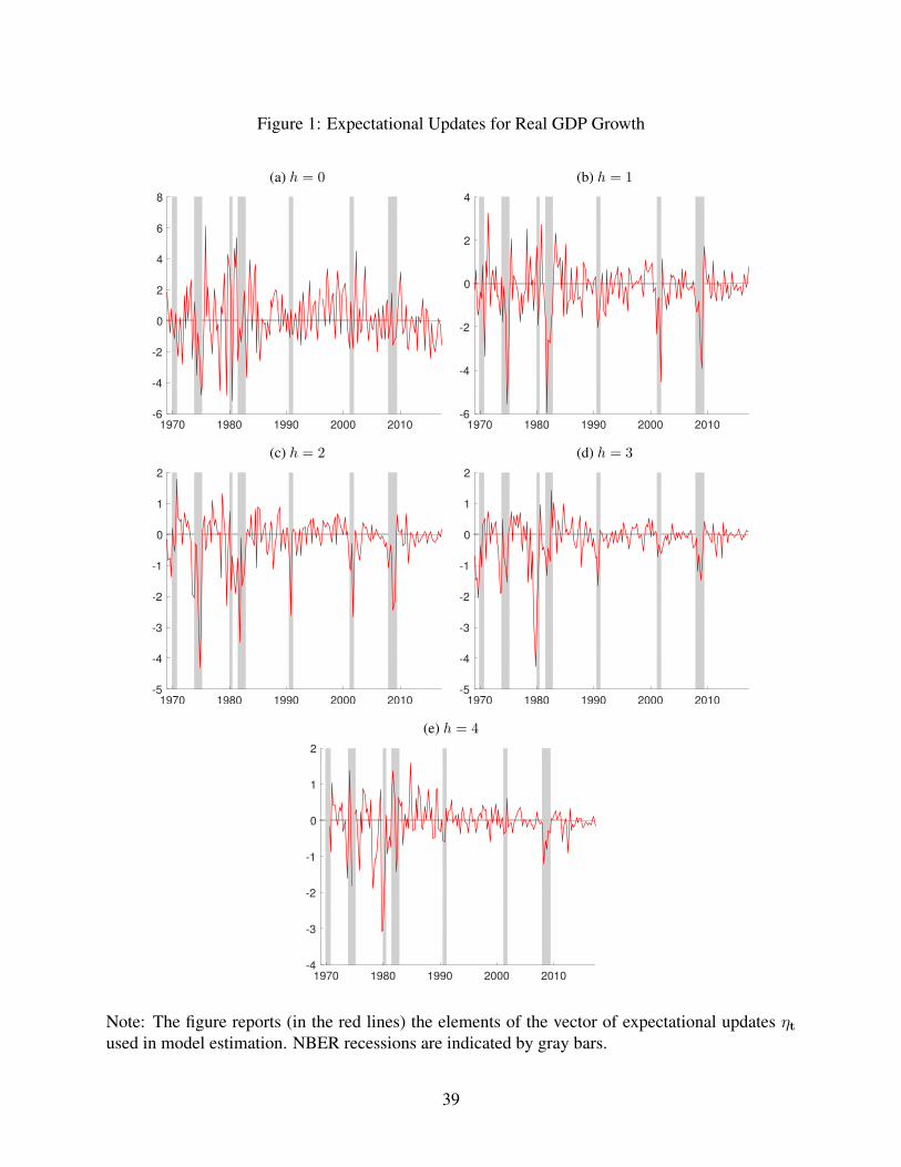
Figure 1: Expectational Updates for Real GDP Growth

(a) h = 0

1970 1980 1990 2000 2010

-6

-4

-2

0

2

4

6

8

(b) h = 1

1970 1980 1990 2000 2010

-6

-4

-2

0

2

4

(c) h = 2

1970 1980 1990 2000 2010

-5

-4

-3

-2

-1

0

1

2

(d) h = 3

1970 1980 1990 2000 2010

-5

-4

-3

-2

-1

0

1

2

(e) h = 4

1970 1980 1990 2000 2010

-4

-3

-2

-1

0

1

2

Note: The figure reports (in the red lines) the elements of the vector of expectational updates ηtused in model estimation. NBER recessions are indicated by gray bars.

39

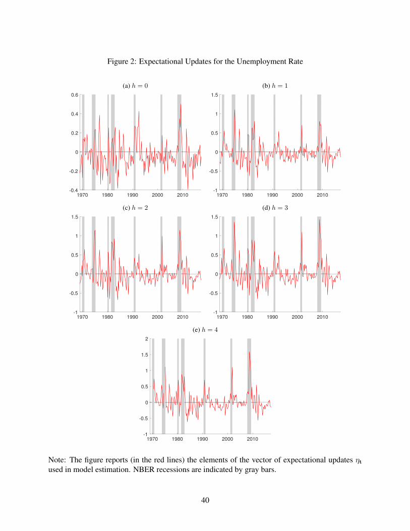
Figure 2: Expectational Updates for the Unemployment Rate

(a) h = 0

1970 1980 1990 2000 2010

-0.4

-0.2

0

0.2

0.4

0.6

(b) h = 1

1970 1980 1990 2000 2010

-1

-0.5

0

0.5

1

1.5

(c) h = 2

1970 1980 1990 2000 2010

-1

-0.5

0

0.5

1

1.5

(d) h = 3

1970 1980 1990 2000 2010

-1

-0.5

0

0.5

1

1.5

(e) h = 4

1970 1980 1990 2000 2010

-1

-0.5

0

0.5

1

1.5

2

Note: The figure reports (in the red lines) the elements of the vector of expectational updates ηtused in model estimation. NBER recessions are indicated by gray bars.

40

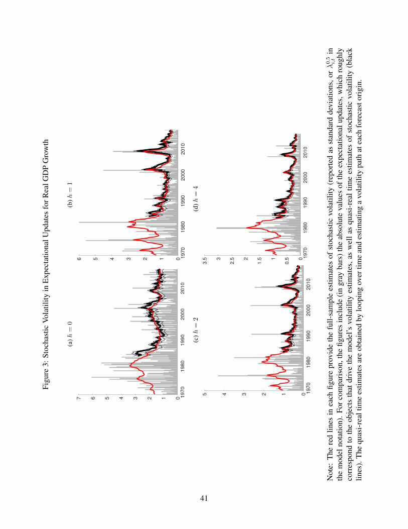
Figu

re3:

Stoc

hast

icVo

latil

ityin

Exp

ecta

tiona

lUpd

ates

forR

ealG

DP

Gro

wth

(a)h

=0

1970

1980

1990

2000

2010

01234567

(b)h

=1

1970

1980

1990

2000

2010

0123456

(c)h

=2

1970

1980

1990

2000

2010

012345

(d)h

=4

19

70

19

80

19

90

20

00

20

10

0

0.51

1.52

2.53

3.5

Not

e:T

here

dlin

esin

each

figur

epr

ovid

eth

efu

ll-sa

mpl

ees

timat

esof

stoc

hast

icvo

latil

ity(r

epor

ted

asst

anda

rdde

viat

ions

,orλ0.5

i,t

inth

em

odel

nota

tion)

.Fo

rco

mpa

riso

n,th

efig

ures

incl

ude

(in

gray

bars

)the

abso

lute

valu

esof

the

expe

ctat

iona

lupd

ates

,whi

chro

ughl

yco

rres

pond

toth

eob

ject

sth

atdr

ive

the

mod

el’s

vola

tility

estim

ates

,as

wel

las

quas

i-re

altim

ees

timat

esof

stoc

hast

icvo

latil

ity(b

lack

lines

).T

hequ

asi-

real

time

estim

ates

are

obta

ined

bylo

opin

gov

ertim

ean

des

timat

ing

avo

latil

itypa

that

each

fore

cast

orig

in.

41

Figu

re4:

Stoc

hast

icVo

latil

ityin

Exp

ecta

tiona

lUpd

ates

fort

heU

nem

ploy

men

tRat

e

(a)h

=0

19

70

19

80

19

90

20

00

20

10

0

0.1

0.2

0.3

0.4

0.5

0.6

(b)h

=1

19

70

19

80

19

90

20

00

20

10

0

0.2

0.4

0.6

0.81

1.2

(c)h

=2

19

70

19

80

19

90

20

00

20

10

0

0.2

0.4

0.6

0.81

1.2

(d)h

=4

19

70

19

80

19

90

20

00

20

10

0

0.2

0.4

0.6

0.81

1.2

1.4

1.6

Not

e:T

here

dlin

esin

each

figur

epr

ovid

eth

efu

ll-sa

mpl

ees

timat

esof

stoc

hast

icvo

latil

ity(r

epor

ted

asst

anda

rdde

viat

ions

,orλ0.5

i,t

inth

em

odel

nota

tion)

.Fo

rco

mpa

riso

n,th

efig

ures

incl

ude

(in

gray

bars

)the

abso

lute

valu

esof

the

expe

ctat

iona

lupd

ates

,whi

chro

ughl

yco

rres

pond

toth

eob

ject

sth

atdr

ive

the

mod

el’s

vola

tility

estim

ates

,as

wel

las

quas

i-re

altim

ees

timat

esof

stoc

hast

icvo

latil

ity(b

lack

lines

).T

hequ

asi-

real

time

estim

ates

are

obta

ined

bylo

opin

gov

ertim

ean

des

timat

ing

avo

latil

itypa

that

each

fore

cast

orig

in.

42

Figu

re5:

Stoc

hast

icVo

latil

ityin

Exp

ecta

tiona

lUpd

ates

forG

DP

Defl

ator

Infla

tion

(a)h

=0

19

70

19

80

19

90

20

00

20

10

0

0.51

1.52

2.53

3.54

(b)h

=1

19

70

19

80

19

90

20

00

20

10

0

0.51

1.52

2.5

(c)h

=2

19

70

19

80

19

90

20

00

20

10

0

0.51

1.52

(d)h

=4

19

70

19

80

19

90

20

00

20

10

0

0.2

0.4

0.6

0.81

1.2

1.4

1.6

Not

e:T

here

dlin

esin

each

figur

epr

ovid

eth

efu

ll-sa

mpl

ees

timat

esof

stoc

hast

icvo

latil

ity(r

epor

ted

asst

anda

rdde

viat

ions

,orλ0.5

i,t

inth

em

odel

nota

tion)

.Fo

rco

mpa

riso

n,th

efig

ures

incl

ude

(in

gray

bars

)the

abso

lute

valu

esof

the

expe

ctat

iona

lupd

ates

,whi

chro

ughl

yco

rres

pond

toth

eob

ject

sth

atdr

ive

the

mod

el’s

vola

tility

estim

ates

,as

wel

las

quas

i-re

altim

ees

timat

esof

stoc

hast

icvo

latil

ity(b

lack

lines

).T

hequ

asi-

real

time

estim

ates

are

obta

ined

bylo

opin

gov

ertim

ean

des

timat

ing

avo

latil

itypa

that

each

fore

cast

orig

in.

43

Figu

re6:

Stoc

hast

icVo

latil

ityin

Exp

ecta

tiona

lUpd

ates

forC

PIIn

flatio

n

(a)h

=0

1985

1990

1995

2000

2005

2010

2015

01234567

(b)h

=1

1985

1990

1995

2000

2005

201

02015

0123456

(c)h

=2

19

85

19

90

19

95

20

00

20

05

20

10

20

15

0

0.51

1.52

2.5

(d)h

=4

19

85

19

90

19

95

20

00

20

05

20

10

20

15

0

0.2

0.4

0.6

0.81

1.2

1.4

1.6

Not

e:T

here

dlin

esin

each

figur

epr

ovid

eth

efu

ll-sa

mpl

ees

timat

esof

stoc

hast

icvo

latil

ity(r

epor

ted

asst

anda

rdde

viat

ions

,orλ0.5

i,t

inth

em

odel

nota

tion)

.Fo

rco

mpa

riso

n,th

efig

ures

incl

ude

(in

gray

bars

)the

abso

lute

valu

esof

the

expe

ctat

iona

lupd

ates

,whi

chro

ughl

yco

rres

pond

toth

eob

ject

sth

atdr

ive

the

mod

el’s

vola

tility

estim

ates

,as

wel

las

quas

i-re

altim

ees

timat

esof

stoc

hast

icvo

latil

ity(b

lack

lines

).T

hequ

asi-

real

time

estim

ates

are

obta

ined

bylo

opin

gov

ertim

ean

des

timat

ing

avo

latil

itypa

that

each

fore

cast

orig

in.

44

Figu

re7:

Stoc

hast

icVo

latil

ityin

Exp

ecta

tiona

lUpd

ates

fort

heT

hree

-Mon

thT

bill

Rat

e

(a)h

=0

19

85

19

90

19

95

20

00

20

05

20

10

20

15

0

0.2

0.4

0.6

0.81

(b)h

=1

19

85

19

90

19

95

20

00

20

05

20

10

20

15

0

0.51

1.52

2.53

(c)h

=2

19

85

19

90

19

95

20

00

20

05

20

10

20

15

0

0.51

1.52

2.53

3.5

(d)h

=4

19

85

19

90

19

95

20

00

20

05

20

10

20

15

0

0.51

1.52

2.53

3.5

Not

e:T

here

dlin

esin

each

figur

epr

ovid

eth

efu

ll-sa

mpl

ees

timat

esof

stoc

hast

icvo

latil

ity(r

epor

ted

asst

anda

rdde

viat

ions

,orλ0.5

i,t

inth

em

odel

nota

tion)

.Fo

rco

mpa

riso

n,th

efig

ures

incl

ude

(in

gray

bars

)the

abso

lute

valu

esof

the

expe

ctat

iona

lupd

ates

,whi

chro

ughl

yco

rres

pond

toth

eob

ject

sth

atdr

ive

the

mod

el’s

vola

tility

estim

ates

,as

wel

las

quas

i-re

altim

ees

timat

esof

stoc

hast

icvo

latil

ity(b

lack

lines

).T

hequ

asi-

real

time

estim

ates

are

obta

ined

bylo

opin

gov

ertim

ean

des

timat

ing

avo

latil

itypa

that

each

fore

cast

orig

in.

45

Figu

re8:

Ex-

Ant

eU

ncer

tain

tyB

ands

and

Ex-

Post

Fore

cast

Err

ors

forR

ealG

DP

Gro

wth

(a)h

=0

1985

1990

1995

2000

2005

2010

2015

-3-2-1

012345

(b)h

=1

1985

1990

1995

2000

2005

2010

2015

-6-4-2

0246

(c)h

=2

1985

1990

1995

2000

2005

2010

2015

-8-6-4-2

0246

(d)h

=4

19

85

19

90

19

95

20

00

20

05

20

10

20

15

-10-5

05

Not

e:E

ach

figur

ere

port

sfo

reca

ster

rors

for

each

vari

able

alon

gw

ithon

e-st

anda

rdde

viat

ion

confi

denc

ein

terv

als,

one

set

(in

blue

)ob

tain

edw

ithth

eco

nsta

ntva

rian

ceap

proa

chan

da

60ob

serv

atio

nro

lling

win

dow

ofob

serv

atio

nsan

dth

eot

her(

inre

d)ob

tain

edfr

omou

rsto

chas

ticvo

latil

itym

odel

.

46

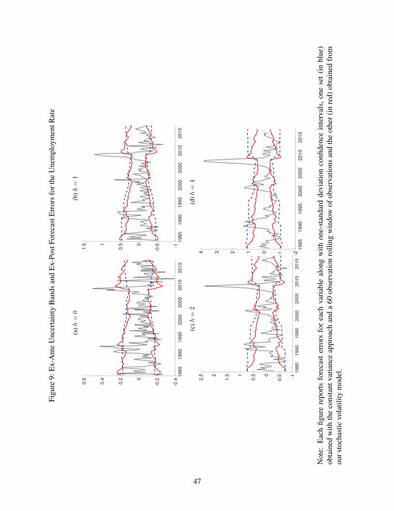
Figu

re9:

Ex-

Ant

eU

ncer

tain

tyB

ands

and

Ex-

Post

Fore

cast

Err

ors

fort

heU

nem

ploy

men

tRat

e

(a)h

=0

19

85

19

90

19

95

20

00

20

05

20

10

20

15

-0.4

-0.20

0.2

0.4

0.6

(b)h

=1

19

85

19

90

19

95

20

00

20

05

20

10

20

15

-1

-0.50

0.51

1.5

(c)h

=2

19

85

19

90

19

95

20

00

20

05

20

10

20

15

-1

-0.50

0.51

1.52

2.5

(d)h

=4

1985

1990

1995

2000

2005

2010

2015

-2-1

01234

Not

e:E

ach

figur

ere

port

sfo

reca

ster

rors

for

each

vari

able

alon

gw

ithon

e-st

anda

rdde

viat

ion

confi

denc

ein

terv

als,

one

set

(in

blue

)ob

tain

edw

ithth

eco

nsta

ntva

rian

ceap

proa

chan

da

60ob

serv

atio

nro

lling

win

dow

ofob

serv

atio

nsan

dth

eot

her(

inre

d)ob

tain

edfr

omou

rsto

chas

ticvo

latil

itym

odel

.

47

Figu

re10

:Ex-

Ant

eU

ncer

tain

tyB

ands

and

Ex-

Post

Fore

cast

Err

ors

forG

DP

Defl

ator

Infla

tion

(a)h

=0

1985

1990

1995

2000

2005

2010

2015

-3-2-1

0123

(b)h

=1

1985

1990

1995

2000

2005

2010

2015

-3-2-1

0123

(c)h

=2

1985

1990

1995

2000

2005

2010

2015

-3-2-1

0123

(d)h

=4

1985

1990

1995

2000

2005

2010

2015

-4-3-2-1

01234

Not

e:E

ach

figur

ere

port

sfo

reca

ster

rors

for

each

vari

able

alon

gw

ithon

e-st

anda

rdde

viat

ion

confi

denc

ein

terv

als,

one

set

(in

blue

)ob

tain

edw

ithth

eco

nsta

ntva

rian

ceap

proa

chan

da

60ob

serv

atio

nro

lling

win

dow

ofob

serv

atio

nsan

dth

eot

her(

inre

d)ob

tain

edfr

omou

rsto

chas

ticvo

latil

itym

odel

.

48

Figu

re11

:Ex-

Ant

eU

ncer

tain

tyB

ands

and

Ex-

Post

Fore

cast

Err

ors

forC

PIIn

flatio

n

(a)h

=0

19

97

20

00

20

02

20

05

20

07

20

10

20

12

20

15

-8-6-4-2

024

(b)h

=1

19

97

20

00

20

02

20

05

20

07

20

10

20

12

20

15

-15

-10-5

05

(c)h

=2

19

97

20

00

20

02

20

05

20

07

20

10

20

12

20

15

-15

-10-5

05

10

(d)h

=4

19

97

20

00

20

02

20

05

20

07

20

10

20

12

20

15

-15

-10-5

05

10

Not

e:E

ach

figur

ere

port

sfo

reca

ster

rors

for

each

vari

able

alon

gw

ithon

e-st

anda

rdde

viat

ion

confi

denc

ein

terv

als,

one

set

(in

blue

)ob

tain

edw

ithth

eco

nsta

ntva

rian

ceap

proa

chan

da

60ob

serv

atio

nro

lling

win

dow

ofob

serv

atio

nsan

dth

eot

her(

inre

d)ob

tain

edfr

omou

rsto

chas

ticvo

latil

itym

odel

.

49

Figu

re12

:Ex-

Ant

eU

ncer

tain

tyB

ands

and

Ex-

Post

Fore

cast

Err

ors

fort

heT

hree

-Mon

thT

bill

Rat

e

(a)h

=0

1997

2000

2002

2005

2007

2010

2012

2015

-0.6

-0.4

-0.20

0.2

0.4

(b)h

=1

1997

2000

2002

2005

2007

2010

2012

2015

-2

-1.5-1

-0.50

0.51

(c)h

=2

19

97

20

00

20

02

20

05

20

07

20

10

20

12

20

15

-3-2-1

012

(d)h

=4

19

97

20

00

20

02

20

05

20

07

20

10

20

12

20

15

-4-3-2-1

0123

Not

e:E

ach

figur

ere

port

sfo

reca

ster

rors

for

each

vari

able

alon

gw

ithon

e-st

anda

rdde

viat

ion

confi

denc

ein

terv

als,

one

set

(in

blue

)ob

tain

edw

ithth

eco

nsta

ntva

rian

ceap

proa

chan

da

60ob

serv

atio

nro

lling

win

dow

ofob

serv

atio

nsan

dth

eot

her(

inre

d)ob

tain

edfr

omou

rsto

chas

ticvo

latil

itym

odel

.

50

Figu

re13

:Ex-

Ant

eU

ncer

tain

tyB

ands

and

Ex-

Post

Fore

cast

Err

ors

forR

ealG

DP

Gro

wth

:Gre

enbo

okFo

reca

sts

(a)h

=0

1985

1990

1995

2000

2005

2010

-6-4-2

0246

(b)h

=1

1985

1990

1995

2000

2005

2010

-8-6-4-2

02468

(c)h

=2

19

85

19

90

19

95

20

00

20

05

20

10

-10-5

05

10

(d)h

=4

19

85

19

90

19

95

20

00

20

05

20

10

-15

-10-5

05

10

15

Not

e:E

ach

figur

ere

port

sfo

reca

ster

rors

for

each

vari

able

alon

gw

ithon

e-st

anda

rdde

viat

ion

confi

denc

ein

terv

als,

one

set

(in

blue

)ob

tain

edw

ithth

eco

nsta

ntva

rian

ceap

proa

chan

da

60ob

serv

atio

nro

lling

win

dow

ofob

serv

atio

nsan

dth

eot

her(

inre

d)ob

tain

edfr

omou

rsto

chas

ticvo

latil

itym

odel

.

51

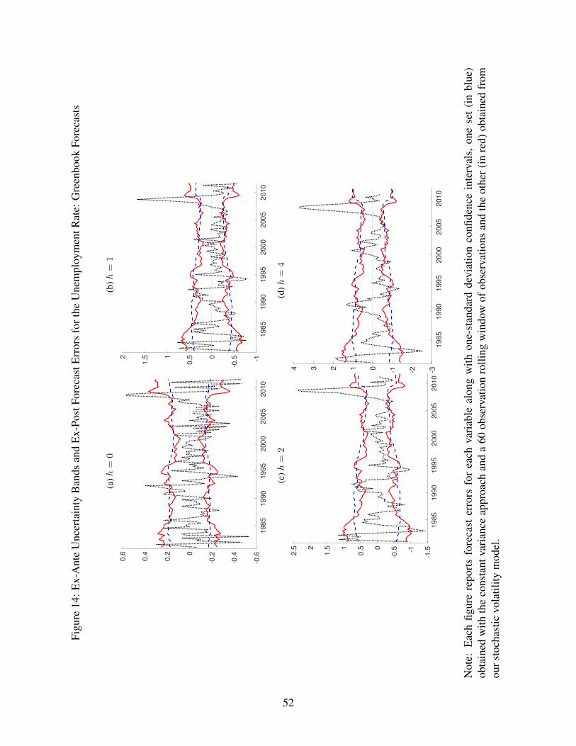
Figu

re14

:Ex-

Ant

eU

ncer

tain

tyB

ands

and

Ex-

Post

Fore

cast

Err

ors

fort

heU

nem

ploy

men

tRat

e:G

reen

book

Fore

cast

s

(a)h

=0

19

85

19

90

19

95

20

00

20

05

20

10

-0.6

-0.4

-0.20

0.2

0.4

0.6

(b)h

=1

19

85

19

90

19

95

20

00

20

05

20

10

-1

-0.50

0.51

1.52

(c)h

=2

19

85

19

90

19

95

20

00

20

05

20

10

-1.5-1

-0.50

0.51

1.52

2.5

(d)h

=4

1985

1990

1995

2000

2005

2010

-3-2-1

01234

Not

e:E

ach

figur

ere

port

sfo

reca

ster

rors

for

each

vari

able

alon

gw

ithon

e-st

anda

rdde

viat

ion

confi

denc

ein

terv

als,

one

set

(in

blue

)ob

tain

edw

ithth

eco

nsta

ntva

rian

ceap

proa

chan

da

60ob

serv

atio

nro

lling

win

dow

ofob

serv

atio

nsan

dth

eot

her(

inre

d)ob

tain

edfr

omou

rsto

chas

ticvo

latil

itym

odel

.

52

Figu

re15

:Ex-

Ant

eU

ncer

tain

tyB

ands

and

Ex-

Post

Fore

cast

Err

ors

forG

DP

Defl

ator

Infla

tion:

Gre

enbo

okFo

reca

sts

(a)h

=0

1985

1990

1995

2000

2005

2010

-5-4-3-2-1

0123

(b)h

=1

1985

1990

1995

2000

2005

2010

-4-3-2-1

0123

(c)h

=2

1985

1990

1995

2000

2005

2010

-3-2-1

0123

(d)h

=4

1985

1990

1995

2000

2005

2010

-6-4-2

024

Not

e:E

ach

figur

ere

port

sfo

reca

ster

rors

for

each

vari

able

alon

gw

ithon

e-st

anda

rdde

viat

ion

confi

denc

ein

terv

als,

one

set

(in

blue

)ob

tain

edw

ithth

eco

nsta

ntva

rian

ceap

proa

chan

da

60ob

serv

atio

nro

lling

win

dow

ofob

serv

atio

nsan

dth

eot

her(

inre

d)ob

tain

edfr

omou

rsto

chas

ticvo

latil

itym

odel

.

53

Figu

re16

:Ex-

Ant

eU

ncer

tain

tyB

ands

and

Ex-

Post

Fore

cast

Err

ors

forC

PIIn

flatio

n:G

reen

book

Fore

cast

s

(a)h

=0

1996

1998

2000

2002

2004

2006

2008

2010

-6-4-2

024

(b)h

=1

19

96

19

98

20

00

20

02

20

04

20

06

20

08

20

10

-15

-10-5

05

(c)h

=2

19

96

19

98

20

00

20

02

20

04

20

06

20

08

20

10

-15

-10-5

05

(d)h

=4

19

96

19

98

20

00

20

02

20

04

20

06

20

08

20

10

-15

-10-5

05

Not

e:E

ach

figur

ere

port

sfo

reca

ster

rors

for

each

vari

able

alon

gw

ithon

e-st

anda

rdde

viat

ion

confi

denc

ein

terv

als,

one

set

(in

blue

)ob

tain

edw

ithth

eco

nsta

ntva

rian

ceap

proa

chan

da

60ob

serv

atio

nro

lling

win

dow

ofob

serv

atio

nsan

dth

eot

her(

inre

d)ob

tain

edfr

omou

rsto

chas

ticvo

latil

itym

odel

.

54