modeling the propagation of computer viruses
TRANSCRIPT
Modeling the propagation of computer viruses
Dr. Stefano Zanero, PhD
Assistant Professor (Ricercatore)Dipartimento di Elettronica e Informazione
Politecnico di [email protected]
S. Zanero (DEI) Modeling the propagation of computer viruses 1 / 41

Lecture Outline
Introduction: computer viruses
History of viruses
Existing models
Graph-based models, file exchange virusesPropagation of e-mail virusesContinuous and discrete models for wormsAdvanced models and issues
Open research questions and conclusions
S. Zanero (DEI) Modeling the propagation of computer viruses 2 / 41
What is a computer virus?
First named by Cohen in [1] and [2]
Research areas in computer virology :
theoretical study of the properties of self-replicating codecreation of new viruses and viral vectorsdevelopment of new techniques for detection and containmentstudy of in-the-wild samples and automation thereofmodeling code replication and propagation behavior
S. Zanero (DEI) Modeling the propagation of computer viruses 3 / 41
A few definitions
Malware: also known as “malicious code”, is code that is intentionallywritten to violate a security policy
Virus: piece of code that self-propagates (i.e. copies itself) byinfecting other files
Worm: self-propagating program which copies itself, often byexploiting host vulnerabilities, or by social engineering (e.g.mail worms)
Trojan horse: program with malicious (e.g. backdoor) capabilities,sometimes masqueraded as benign software
Rootkits: combination of trojans and techniques to hide them
S. Zanero (DEI) Modeling the propagation of computer viruses 4 / 41

A brief history of viruses
1966 von Neumann publishes “Theory of self-reproducingautomata”
1971 Creeper, worm infecting PDP-10 via ARPANET
1974 Wabbit, fork-bomb program; also ANIMAL, a trojan,self-copying program
1981 First reported virus outbreak; first reported boot sector virus:Elk cloner (Apple 2)
1983 Virus definition by Cohen; demonstration of file infection
1986 First PC virus (MS-DOS), Brain (boot sector); VirDemdemoes infection of .com files
1987 First self-encrypting virus (Cascade); first purposefullydestructive virus (Jerusalem, “Friday 13 virus”); SCA, bootsector virus for Amiga
S. Zanero (DEI) Modeling the propagation of computer viruses 5 / 41

A brief history of viruses: the worm age
1988 First self-propagating worm: Morris worm [3]
1989 First multipartite virus: Ghostball
1990 First polymorphic virus: Chameleon
1992 Michelangelo: mass-media hysteria on timebomb
1995 “Concept”, first macro virus
1998 Back orifice; CIH destructive massmailer
1999 Melissa virus (Word+Outlook MM); Knark rootkit; conceptof “zombie”; Happy99 worm email attachment
2000 Loveletter worm
2001 Sadmind worm (Sun+MS IIS); Code Red Worm; Nimda andSircam Worm (multihole)
2003 SQL Slammer worm (UDP!); Blaster worm
S. Zanero (DEI) Modeling the propagation of computer viruses 6 / 41

A brief history of viruses: 2004, annus horribilis
2004 MyDoom, record massmailing worm; Witty worm (multihole,exploits security product, fastest disclosure-to-worm, firstdestructive, limited impact); Sasses worm, last huge UDPworm; Santy is the first webworm
2006 First MacOSX trojan
2007 Storm, massmailer, creates the Storm botnet. At June 30,1.7M computers in it.
2008 Mocmex trojan found in digital photoframe; Torpig (trojan,anti-antivirus) creates a botnet which is later taken over anddestroyed by researchers; Conficker worm infects millions ofmachines creating a botnet; Koobface, facebook andmyspace worm
2009 Scareware and fake-av success
2010 Stuxnet: SCADA trojan; likely targeted
S. Zanero (DEI) Modeling the propagation of computer viruses 7 / 41
Viral code propagation
Viruses need a way to infect a host program, a way to executethemselves when the program is run, and a way to propagate
Common method of propagation in the 80s: floppy disk exchangeCavity infection, appending, prepending; boot code infectionMacro viruses extremely similar
Worms need only a way to propagate and a way to executethemselves automatically
Propagation: social engineering (in particular massmailing) orexploitationExecution through persistent infection of the system
S. Zanero (DEI) Modeling the propagation of computer viruses 8 / 41
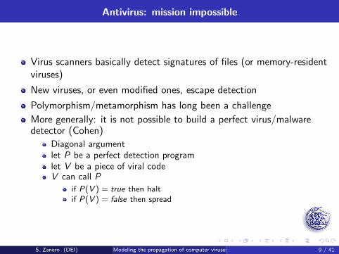
Antivirus: mission impossible
Virus scanners basically detect signatures of files (or memory-residentviruses)
New viruses, or even modified ones, escape detection
Polymorphism/metamorphism has long been a challenge
More generally: it is not possible to build a perfect virus/malwaredetector (Cohen)
Diagonal argumentlet P be a perfect detection programlet V be a piece of viral codeV can call P
if P(V ) = true then haltif P(V ) = false then spread
S. Zanero (DEI) Modeling the propagation of computer viruses 9 / 41
Motivation for creating viral propagation models
Creating reliable models is beneficial for many reasons
It allows to better understand the threat posed by new attack vectorand new propagation techniques. Use of models of worm propagationallowed to predict with a stunning precision the behavior of futuremalware [4]It allows to develop and test improved containment and disinfectionstrategies [5]Combined with load modelling, such models help to predict failures ofthe global network infrastructureSuch models can be used to develop early detection mechanisms bydescribing characteristic symptoms of worm activity (e.g. asymptomatic propagation curve)
For a review (missing out some of the newest developments) see [6]
For an older review of models see [7].
S. Zanero (DEI) Modeling the propagation of computer viruses 10 / 41
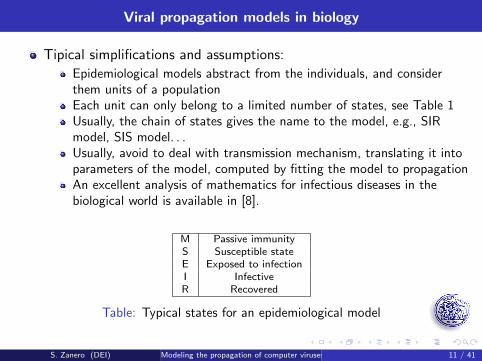
Viral propagation models in biology
Tipical simplifications and assumptions:
Epidemiological models abstract from the individuals, and considerthem units of a populationEach unit can only belong to a limited number of states, see Table 1Usually, the chain of states gives the name to the model, e.g., SIRmodel, SIS model. . .Usually, avoid to deal with transmission mechanism, translating it intoparameters of the model, computed by fitting the model to propagationAn excellent analysis of mathematics for infectious diseases in thebiological world is available in [8].
M Passive immunityS Susceptible stateE Exposed to infectionI InfectiveR Recovered
Table: Typical states for an epidemiological model
S. Zanero (DEI) Modeling the propagation of computer viruses 11 / 41

Modeling file infectors
First model, developed in [9]Tries to overcome two limitations of tipical biological models:
being homogeneous, i.e. an infected individual is equally likely to infectany other individualbeing symmetric, which means that there is no privileged direction oftransmission
Tipically, file exchange happened in cliques and with a specificdirection of flowBoth shortcomings addressed by transferring a SIS model onto adirected random graphimportant effects of the topology of the graph on propagation
Sparse graph (node with small, constant average degree) allows forconditions where infection dies outLocal graph (where probability of having a vertex between nodes Band C is significantly higher if both have a vertex connected to thesame node A), shows higher propagation rate
SIR model would have been interesting to study for file infectors; butthe appearance of the Internet changed the system. . .
S. Zanero (DEI) Modeling the propagation of computer viruses 12 / 41
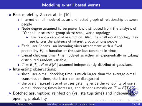
Modeling e-mail based worms
Best model by Zou et al. in [10]Internet e-mail modeled as an undirected graph of relationship betweenpeopleNode degree assumed to be power law distributed from the analysis of“Yahoo!” discussion group sizes; small world topology
This is not a very solid assumption. Also, the small world topology theyuse ignores the existence of interest groups among people
Each user “opens” an incoming virus attachment with a fixedprobability Pi , a function of the user but constant in time.E-mail checking time Ti is modeled as either an exponentially or Erlangdistributed random variable.T = E [Ti ], P = E [Pi ] assumed independently distributed gaussians.
Interesting observations:since user e-mail checking time is much larger than the average e-mailtransmission time, the latter can be disregardedthe overall spread rate of viruses gets higher as the variability of users’e-mail checking times increases, and depends mostly on T = E [Ti ]
Botched assumption: reinfection (vs. startup time) and independentopening probability
S. Zanero (DEI) Modeling the propagation of computer viruses 13 / 41

Modeling scanning worms
Random Constant Spread (RCS) model [4]
Developed using empirical data derived from the outbreak of theCode Red v2 worm
Released in version 1 on 13 Jul 2001 and immediately analyzed [11, 12]Propagates using the .ida vulnerability discovered by eEye on June18th 2001 [13], thus infecting vulnerable web servers running MicrosoftIIS version 4.0 and 5.0.On the infected host it launches 99 threads, which randomly generateIP addresses (excluding subnets 127.0.0.0/8, loopback, and224.0.0.0/8, multicast) and try to compromise the hosts at thoseaddressesversion 1 had flawed random number generator; version 2 fixes this andadds subroutine for DDoS attack against www1.whitehouse.gov onthe days between the 20th and the 28th of each month, thenreactivating on the 1st of the following month.No resident infection: a simple reboot eliminates it, but allowsreinfection. Patching makes instead the machine invulnerable toreinfection.
S. Zanero (DEI) Modeling the propagation of computer viruses 14 / 41

The RCS model
Let N be the total number of vulnerable servers which can bepotentially compromised from the Internet
ignores that systems can be patched, powered and shut down, deployedor disconnectedignores target networks behind NAT devicesignores that recent researches as much as the 5% of the routed (andused) address space is not reachable by various portions of thenetwork [14]
Let K be the average compromise rate, i.e. the number of vulnerablehosts that an infected host can compromise per unit of time
The model assumes that K is constantAssumes that a machine cannot be compromised multiple times
Let a(t) be the share of vulnerable machines which have beencompromised at the instant t
Then it follows that the number n of machines that will becompromised in the interval dt is:
n = (Na) · K (1 − a)dt
S. Zanero (DEI) Modeling the propagation of computer viruses 15 / 41
The RCS model(2)
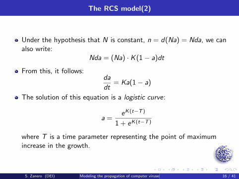
Under the hypothesis that N is constant, n = d(Na) = Nda, we canalso write:
Nda = (Na) · K (1 − a)dt
From this, it follows:da
dt= Ka(1 − a)
The solution of this equation is a logistic curve:
a =eK(t−T )
1 + eK(t−T )
where T is a time parameter representing the point of maximumincrease in the growth.
S. Zanero (DEI) Modeling the propagation of computer viruses 16 / 41
Fitting RCS against CodeRed
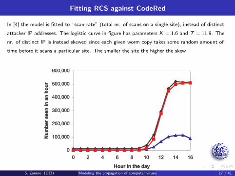
In [4] the model is fitted to “scan rate” (total nr. of scans on a single site), instead of distinct
attacker IP addresses. The logistic curve in figure has parameters K = 1.6 and T = 11.9. The
nr. of distinct IP is instead skewed since each given worm copy takes some random amount of
time before it scans a particular site. The smaller the site the higher the skew
S. Zanero (DEI) Modeling the propagation of computer viruses 17 / 41
Fitting RCS against CodeRed (2)
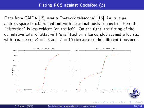
Data from CAIDA [15] uses a “network telescope” [16], i.e. a largeaddress-space block, routed but with no actual hosts connected. Here the“distortion” is less evident (on the left). On the right, the fitting of thecumulative total of attacker IPs is fitted on a loglog plot against a logisticwith parameters K = 1.8 and T = 16 (because of the different timezone).
S. Zanero (DEI) Modeling the propagation of computer viruses 18 / 41
Fitting RCS against CodeRed (3)
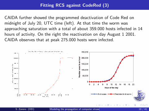
CAIDA further showed the programmed deactivation of Code Red onmidnight of July 20, UTC time (left). At that time the worm wasapproaching saturation with a total of about 359.000 hosts infected in 14hours of activity. On the right the reactivation on day August 1 2001.CAIDA observes that at peak 275.000 hosts were infected.
S. Zanero (DEI) Modeling the propagation of computer viruses 19 / 41
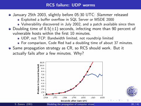
RCS failure: UDP worms
January 25th 2003, slightly before 05:30 UTC: Slammer releasedExploited a buffer overflow in SQL Server or MSDE 2000Vulnerability discovered in July 2002, and a patch available since then
Doubling time of 8.5(±1) seconds, infecting more than 90 percent ofvulnerable hosts within the first 10 minutes.
UDP, not TCP. Bandwidth limited, not roundtrip limitedFor comparison, Code Red had a doubling time of about 37 minutes.
Same propagation strategy as CR, so RCS should work. But itactually fails after a few minutes. Why?
S. Zanero (DEI) Modeling the propagation of computer viruses 20 / 41

Compartment models and understanding the data
We must understand that after 3 minutes, the worm achieved a rateof 55 million scans per second. This affected the Internet:
by slowing down and throttling the scans through bottleneck linksby throttling the observation link
We can build a compartment based model [6]densely connected regions where the worm propagates unhindered,following RCSintra-region propagation with a bottleneck
Denoting with Ni and ai the parameters of a single region, andsupposing K to be constant across all of the n regions: dai
dt =
aiK NiN +
n∑j=1j 6=i
Nj
NiajK
NiN
(1 − ai ) 1 ≤ i ≤ n
Think of the result of the integration of each equation as a logisticfunction somehow “forced” in its growth by the second additive term(which represents the attacks incoming from outside the region)
S. Zanero (DEI) Modeling the propagation of computer viruses 21 / 41
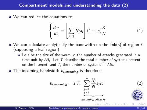
Compartment models and understanding the data (2)
We can reduce the equations to:daidt
=
n∑j=1
Njaj
(1 − ai )K
N(1)
We can calculate analytically the bandwidth on the link(s) of region i(supposing a leaf region)
Le s be the size of the worm, rj the number of attacks generated in atime unit by ASj . Let T describe the total number of systems presenton the Internet, and Ti the number of systems in ASi .
The incoming bandwidth bi ,incoming is therefore:
bi ,incoming = s Ti
n∑j=1j 6=i
Nj
NajK
︸ ︷︷ ︸incoming attacks
(2)
S. Zanero (DEI) Modeling the propagation of computer viruses 22 / 41
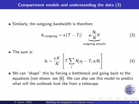
Compartment models and understanding the data (3)
Similarly, the outgoing bandwidth is therefore:
bi ,outgoing = s (T − Ti ) aiNi
NK︸ ︷︷ ︸
outgoing attacks
(3)
The sum is:
bi =s K
N
T ∑j
Njaj − Ti aiNi
(4)
We can “shape” this by forcing a bottleneck and going back to theequations (not shown, see [6]. We can also use this model to predictwhat will the outbreak look like from a telescope.
S. Zanero (DEI) Modeling the propagation of computer viruses 23 / 41

Compartment models and understanding the data (4)
Figure: A comparison between the unrestricted growth predicted by an RCSmodel and the growth restricted by bandwidth constraints, on the left. On theright, the number of attack rates seen by a global network telescope, under thehypothesis that some links fail and saturate during the outbreak
S. Zanero (DEI) Modeling the propagation of computer viruses 24 / 41
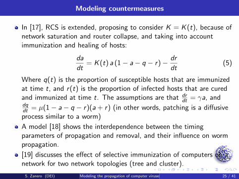
Modeling countermeasures
In [17], RCS is extended, proposing to consider K = K (t), because ofnetwork saturation and router collapse, and taking into accountimmunization and healing of hosts:
da
dt= K (t) a (1 − a− q − r) − dr
dt(5)
Where q(t) is the proportion of susceptible hosts that are immunizedat time t, and r(t) is the proportion of infected hosts that are curedand immunized at time t. The assumptions are that dr
dt = γa, anddqdt = µ(1 − a− q − r)(a + r) (in other words, patching is a diffusiveprocess similar to a worm)
A model [18] shows the interdependence between the timingparameters of propagation and removal, and their influence on wormpropagation.
[19] discusses the effect of selective immunization of computers on anetwork for two network topologies (tree and cluster).
S. Zanero (DEI) Modeling the propagation of computer viruses 25 / 41

Developing new countermeasures from models
In [20] a monitoring and alerting system is proposed, based ondistributed ingress and egress sensors for worm activity. They alsopropose the use of a Kalman filter for estimating parameters such asK , N and a from the observations, and thus have a detailedunderstanding of how much damage the spreading worm couldgenerate. In addition, using some properties of the filter, it can beused to generate and early warning of worm activity as early as when1% ≤ a ≤ 2%.
Quarantine [21] and self-quarantine [22] have been extensivelydiscussed and modeled.
S. Zanero (DEI) Modeling the propagation of computer viruses 26 / 41

Modeling Bluetooth worms
Bluetooth standard enables close range transmission of files
Worm propagation problemPotential for attacks
A huge number of people crying wolf (and sellingwolf-protection-systems, which makes them less credible. . . )
Modeling and assessing the threat is difficult, because of localityissues
Despite claims, no one has performed serious studies on this (hint toreviewers: please, don’t just google it up and see the number of thehits. . . )
S. Zanero (DEI) Modeling the propagation of computer viruses 27 / 41
A Bluetooth primer
Bluetooth is a short range short-wave radio communication protocol
Alternative to IrDA, no line of sight required
This creates a potential for worm transmission. Woo-hoo!
Range between 1-100m, most devices 10m
Robust security and crypto mechanisms
Also, you cannot sniff on common hw because of pseudorandomhopping
Unluckily, plethora of implementation bugs, leading to DoS,command execution, etc.
Worms reportedly exist:
Propagation through an OBEX push connection (e.g. Cabir [23])Multidropper worms targeting both PC and cellphone
. . . do they, actually?
S. Zanero (DEI) Modeling the propagation of computer viruses 28 / 41

First research effort: BlueBag
S. Zanero (DEI) Modeling the propagation of computer viruses 29 / 41

Worm propagation modeling
Used CMMTool to emulate movements
Omitted layer-1 aspects and shielding (this was a bad assumption aswe will see)
Used real environment characteristics and data collected during oursurvey to create scenarios
Gave scary estimates of propagation speed and probability [24]
We are now creating BlueBat, an experimental honeypot forBluetooth attacks
S. Zanero (DEI) Modeling the propagation of computer viruses 30 / 41
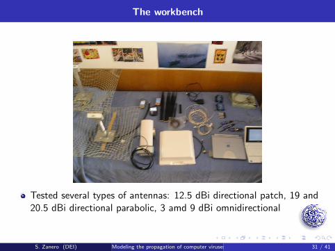
The workbench
Tested several types of antennas: 12.5 dBi directional patch, 19 and20.5 dBi directional parabolic, 3 amd 9 dBi omnidirectional
S. Zanero (DEI) Modeling the propagation of computer viruses 31 / 41

Ranges, ranges . . .
Range tests [25]Two class 2 phones, open space, range approximately 20mClass 1 dongle (without an antenna) and phone, open space, approx60mLinksys dongle with external antenna and phone, open space, approx90mAircable dongle, open space, 110m (with a 3dBi omnidirectionalantenna), 175m (9 dBi omnidirectional antenna), 400m (12.5 dBipatch antenna), 1.48Km (20.5 dbi parabolic antenna).
S. Zanero (DEI) Modeling the propagation of computer viruses 32 / 41
In the wild results
Days of observation in crowded places in Milan, plus 6 months ofcontinuous operation of 2 portable devices
Hundreds of visible devices passed by
A total of 3 files were received:
sarah.jpeg (do I actually need to explain what this is?)Leading brand of footwear commercialUnknown .sis file (485zp6x6 .sis, an executable for the Symbianplatform (corrupt. . . )
Trying to push an innocuous file: 6%–8% of individuals carelesslyaccept unknown file transfers from unknown sources. This didn’tchange from BlueBag in 2006 to BlueBat in 2008.
S. Zanero (DEI) Modeling the propagation of computer viruses 33 / 41
Models and open questions
A number of models have been proposed for Bluetooth wormpropagation, almost invariably showing great propagation potentials[26, 24, 27, 28].
This potential failed to materialize, in our opinion because of thedifficulty of casual transmission. This was actually predicted in [29],which went against the common perception that mobility helpedspreading such worms [27].
“Human shield” effect!
Low-level description of transmission may not be the best approach;we are thinking of using a model based on scale-free networks
. . . 30 years later, we are back to propagations over graphs!
S. Zanero (DEI) Modeling the propagation of computer viruses 34 / 41
References I
[1] Fred Cohen.
Computer Viruses.
PhD thesis, University of Southern California, 1985.
[2] Fred Cohen.
Computer viruses – theory and experiments.
Computers & Security, 6(1):22–35, 1987.
[3] E. H. Spafford.
Crisis and aftermath.
Communications of the ACM, 32(6):678–687, 1989.
[4] Stuart Staniford, Vern Paxson, and Nicholas Weaver.
How to 0wn the internet in your spare time.
In Proceedings of the 11th USENIX Security Symposium (Security ’02), 2002.
S. Zanero (DEI) Modeling the propagation of computer viruses 35 / 41
References II
[5] Ian Whalley, Bill Arnold, David Chess, John Morar, Alla Segal, and MortonSwimmer.
An environment for controlled worm replication and analysis.
In Proceedings of the Virus Bulletin Conference, September 2000.
[6] Giuseppe Serazzi and Stefano Zanero.
Computer virus propagation models.
In Mariacarla Calzarossa and Erol Gelenbe, editors, Performance Tools andApplications to Networked Systems, Revised Tutorial Lectures [from MASCOTS2003], volume 2965 of Lecture Notes in Computer Science, pages 26–50. Springer,2004.
[7] Steve R. White.
Open problems in computer virus research.
In Proceedings of the Virus Bulletin Conference, Oct 1998.
[8] Herbert W. Hethcote.
The mathematics of infectious diseases.
SIAM Review, 42(4):599–653, 2000.
S. Zanero (DEI) Modeling the propagation of computer viruses 36 / 41

References III
[9] J. O. Kephart and S. R. White.
Directed-graph epidemiological models of computer viruses.
In IEEE Symposium on Security and Privacy, pages 343–361, 1991.
[10] Cliff Changchun Zou, Don Towsley, and Weibo Gong.
Email virus propagation modeling and analysis.
Technical Report TR-CSE-03-04, University of Massachussets, Amherst.
[11] Ryan Permeh and Marc Maiffret.
.ida ’code red’ worm.
Advisory AL20010717, July 2001.
[12] Ryan Permeh and Marc Maiffret.
Code red disassembly.
Assembly code and research paper, July 2001.
[13] Ryan Permeh and Riley Hassell.
Microsoft i.i.s. remote buffer overflow.
Advisory AD20010618, June 2001.
S. Zanero (DEI) Modeling the propagation of computer viruses 37 / 41
References IV
[14] Abha Ahuja Craig Labovitz and Michael Bailey.
Shining light on dark address space.
Technical report, Arbor networks, Nov 2001.
[15] David Moore, Colleen Shannon, and Jeffery Brown.
Code-red: a case study on the spread and victims of an internet worm.
In Proceedings of the ACM SIGCOMM/USENIX Internet Measurement Workshop,Nov 2002.
[16] David Moore.
Network telescopes: Observing small or distant security events.
In Proceedings of the 11th USENIX Security Symposium, Aug 2002.
[17] Cliff Changchun Zou, Weibo Gong, and Don Towsley.
Code red worm propagation modeling and analysis.
In Proceedings of the 9th ACM conference on Computer and communicationssecurity, pages 138–147. ACM Press, 2002.
S. Zanero (DEI) Modeling the propagation of computer viruses 38 / 41

References V
[18] Yang Wang and Chenxi Wang.
Modelling the effects of timing parameters on virus propagation.
In Proceedings of the ACM CCS Workshop on Rapid Malcode (WORM’03), Oct2003.
[19] Chenxi Wang, J. C. Knight, and M. C. Elder.
On computer viral infection and the effect of immunization.
In ACSAC, pages 246–256, 2000.
[20] Cliff Changchun Zou, Lixin Gao, Weibo Gong, and Don Towsley.
Monitoring and early warning for internet worms.
In Proceedings of the 10th ACM conference on Computer and communicationsecurity, pages 190–199. ACM Press, 2003.
[21] David Moore, Colleen Shannon, Geoffrey M. Voelker, and Stefan Savage.
Internet quarantine: Requirements for containing self-propagating code.
In INFOCOM, 2003.
S. Zanero (DEI) Modeling the propagation of computer viruses 39 / 41

References VI
[22] Cliff Changchun Zou, Weibo Gong, and Don Towsley.
Worm propagation modeling and analysis under dynamic quarantine defense.
In Proceedings of the ACM CCS Workshop on Rapid Malcode (WORM’03), Oct2003.
[23] Cabir.
Analysis available online at http://www.symantec.com/security_response/writeup.jsp?docid=2004-061419-4412-99.
[24] Luca Carettoni, Claudio Merloni, and Stefano Zanero.
Studying bluetooth malware propagation: The bluebag project.
IEEE Security and Privacy, 5(2):17–25, 2007.
[25] A. Galante, A. Kokos, and S. Zanero.
Bluebat: Towards practical bluetooth honeypots.
In 2009 IEEE International Conference on Communications, Dresden, Germany,June 2009.
S. Zanero (DEI) Modeling the propagation of computer viruses 40 / 41
References VII
[26] Jing Su, Kelvin K. W. Chan, Andrew G. Miklas, Kenneth Po, Ali Akhavan, StefanSaroiu, Eyal de Lara, and Ashvin Goel.
A preliminary investigation of worm infections in a bluetooth environment.
In WORM ’06: Proceedings of the 4th ACM workshop on Recurring malcode,pages 9–16, New York, NY, USA, 2006. ACM.
[27] James W. Mickens and Brian D. Noble.
Modeling epidemic spreading in mobile environments.
In WiSe ’05: Proceedings of the 4th ACM workshop on Wireless security, pages77–86, New York, NY, USA, 2005. ACM.
[28] Guanhua Yan and Stephan Eidenbenz.
Modeling propagation dynamics of bluetooth worms (extended version).
IEEE Transactions on Mobile Computing, 8(3):353–368, 2009.
[29] Guanhua Yan and Stephan Eidenbenz.
Bluetooth worms: Models, dynamics, and defense implications.
In ACSAC ’06: Proceedings of the 22nd Annual Computer Security ApplicationsConference, pages 245–256, Washington, DC, USA, 2006. IEEE Computer Society.
S. Zanero (DEI) Modeling the propagation of computer viruses 41 / 41