modeling the mechanisms underlying the formation …
TRANSCRIPT

MODELING THE MECHANISMS UNDERLYING THE FORMATION OF
COLLAGEN-MIMETIC TRIPLE HELICES AND MICROFIBRILS
By
VYSHNAVI S. KARRA
A thesis submitted to the
Graduate School – New Brunswick
Rutgers, The State University of New Jersey
In partial fulfillment of the requirements
For the degree of
Master of Science
Graduate Program in Chemical and Biochemical Engineering
Written under the direction of
Dr. Meenakshi Dutt
And approved by
_________________________________________
_________________________________________
_________________________________________
New Brunswick, New Jersey
October, 2017
ii
ABSTRACT OF THE THESIS
Modeling the Mechanisms Underlying the Formation of Collagen-Mimetic Triple Helices
and Microfibrils
By VYSHNAVI S. KARRA
Thesis Director:
Dr. Meenakshi Dutt
Collagen is an abundant and integral protein within the body, due to its mechanical strength
and elastisticity. These properties arise from the structural hierarchy of collagen, from the
peptide strands, to tropocollagen, to microfibrils, to fibers. Understanding the formation
mechanisms of collagen can aid in the research of various collagen related disorders, such
as heart disease, skin aging, Oseteogenesis Imperfecta, etc. In this study, we simulated
three short, simplified collagen peptide strands using the MARTINI coarse grained scheme.
Once the tropocollagen was formed, it was replicated five more times and simulated to
form a microfibril. Using mathematical equations of a helix, we characterized the
tropocollagen to have a curvature (κ) of 0.9237 and a torsion (τ) of 0.6395. The maximum
average interaction count occurs between two of the three strands for the tropocollagen at
fifteen, suggesting in partial uncoiling of the triple helix. The average interaction counts
for the microfibril are around eight, suggesting that the formation mechanism is the
individual peptide strands bundling to form a microfibril-like structure, rather than forming
tropocollagens and then microfibrils.

iii
Acknowledgements:
Pursuing an M.S. degree within the past year has been quite an experience, and I
cannot have done as well as I have without the support and help from the Computational
Hybrid Soft Materials Laboratory group members. I would like to thank my thesis advisor,
Dr. Meenakshi Dutt, for her guidance and mentoring for the past four years, both as an
undergraduate and a graduate student.
It is my privilege to have Dr. Nina Shapley and Dr. Wilma Olson as my committee
members. I would like to thank them for accepting my invitation and working to try and
find a suitable date for the thesis defense during their busy summer schedules.
I would like to thank my collaborators – Srinivas Mushnoori, Sarah Libring, and
Brian Ronan – for their help and guidance throughout this project. I would like to thank
Akash Banarjee and Jia Li for their help with the helicity and the interaction counts,
respectively.
I would like to thank XSEDE for the computational resources, using Stampede and
Stampede2 from Texas Advanced Computing Center (TACC) and Bridges from Pittsburge
Supercomputing Center (PSC). In addition, I would like to thank Rutgers Discovery
Informatics Institute (RDI2) for providing access to ELF/Caliburn. I would like to thank
the creators of NLREG for providing a demonstration version of their program.
Finally, I would like to dedicate this thesis to my younger brother, a special needs
individual that always provided the motivation to pursue my academic goals with his
cheerful humor and infinite love.

iv
Table of Contents
ABSTRACT OF THE THESIS...........................................................................................ii
Acknowledgements............................................................................................................iii
Table of Contents................................................................................................................iv
List of Tables.......................................................................................................................v
List of Illustrations..............................................................................................................v
Chapter 1: Introduction.......................................................................................................1
Chapter 2: Background.......................................................................................................8
Chapter 3: Methodology...................................................................................................13
3.1 Molecular Dynamics.......................................................................................13
3.2 Molecular Interaction Potentials.....................................................................15
3.3 Protein Models................................................................................................17
3.4 The Model.......................................................................................................20
Chapter 4: Triple Helix Simulations.................................................................................26
Chapter 5: Microfibril Simulations..................................................................................30
Chapter 6: Results & Discussion......................................................................................33
6.1 Helicity of the Triple Helix............................................................................33
6.2 Interaction Counts..........................................................................................33
Chapter 7: Conclusions.....................................................................................................43
Chapter 8: Future Work....................................................................................................44
Bibliography.....................................................................................................................45
v
List of Tables
Table 1: Types of collagen within the body.......................................................................1
Table 2: Select coarse grain protein models......................................................................17
Table 3: Interaction matrix between all bead subtypes.....................................................22
Table 4: Bead types for glycine, proline and hydroxyproline...........................................23
Table 5: Bond, angle, and dihedral parameters.................................................................23
List of Illustrations
Figure 1: Aging of the arteries............................................................................................3
Figure 2: Collagen bundles in young skin versus old skin.................................................4
Figure 3: Structure of the extracellular matrix...................................................................5
Figure 4: Biosynthetic pathway of collagen formation......................................................6
Figure 5: Structural hierarchy of collagen..........................................................................8
Figure 6: Collagen microfibril structure.............................................................................9
Figure 7: Osteogenesis Imperfecta example......................................................................10
Figure 8: Molecular modeling and applications................................................................14
Figure 9: Bonding potentials and interactions...................................................................16
Figure 10: Comparison of all-atom and coarse-grained modeling....................................19
Figure 11: MARTINI coarse-grained representation........................................................20
Figure 12: MARTINI mapping for 20 amino acids...........................................................21
Figure 13: One peptide strand...........................................................................................24
Figure 14: Initial configuration of three peptide strands...................................................27
Figure 15: Three peptide strands after 120 ns...................................................................28
Figure 16: Three peptide strands after 320 ns...................................................................29
vi
Figure 17: Initial configuration of six tropocollagens.......................................................30
Figure 18: Six tropocollagens after 560 ns........................................................................31
Figure 19: Six tropocollagens after 1.1 μs.........................................................................31
Figure 20: Mean angle for a collagen helix.......................................................................34
Figure 21: Schematic of the calculated angles..................................................................35
Figure 22: Collagen triple helix parameters......................................................................36
Figure 23: Average number of interaction counts for the triple helix...............................39
Figure 24: Average number of interaction counts for the microfibril...............................40
Figure 25: Microfibril system with only the glycine backbone beads..............................41

1
Chapter 1: Introduction
Collagen is one of the most integral proteins in the human body because of its
physical properties: 1) elasticity and 2) mechanical strength and stability. In addition to
these properties, there are at least sixteen types of collagen. However, the majority of all
of the collagen found within the human body are types I, II, and III. Some of the major
collagen types are shown below:
Type Molecular
Composition
Structural Features Representative
Tissues
Fibrillar Collagens
I [α1(I)]2[α2(I)] 300 nm long fibrils Skin, tendon, bone,
ligaments, dentin,
interstitial tissues
II [α1(II)]3 300 nm long fibrils
Cartilage, vitreous
humor
III [α(III)]3 300 nm long fibrils
Often with type I
Skin, muscle, blood
vessels
V [α(V)]3 390 nm long fibrils with globular
N-terminal
Often with type I
Similar to type I
Also cell cultures,
fetal tissues
Fibril-Associated Collagens
VI [α1(VI)][α2(VI)] Lateral association with type I
Periodic globular domains
Most interstitial
tissues
IX [α1(IX)][α2(IX)]
[α3(IX)]
Lateral association with type II
N-terminal globular domain
Bound glycosaminoglycan
Cartilage, vitreous
humor
Sheet-Forming Collagens
IV [α1(IV)]2[α2(IV)] Two dimensional network
All basal lamina
VII [α1(VII)]3 Long fibrils Below basal lamina
of the skin
XV [α1(XV)]3 Core protein of chondroitin sulfate
proteoglycan
Widespread
Near basal lamina in
muscle
Transmembrane Collagens
XIII [α1(XIII)]3 Integral membrane protein
Hemidesmosomes in
skin

2
XVII [α1(XVII)]3 Integral membrane protein Hemidesmosomes in
skin
Host Defense Collagens
Collectins Oligomers of triple helix
Lectin domains
Blood, alveolar space
C1q Oligomers of triple helix
Blood (complement)
Class A scavenger
receptors
Homotrimeric membrane proteins Macrophages
Table 1: Types of collagens with their compositions, primary functions and locations within the body.19
Collagen is found within a plethora of systems within the body, with a multitude of
functions, ranging from macrophages to the vitreous humor, the transparent tissue with
jelly-like consistency that fills the eyeball behind the lens.
Fibrillar collagens are among the most abundant and versatile collagen types.
They are made up of long thin fibrils, which are very fine fibers and can then bundle to
form fibers. These long thin fibrils arise from a triple helix, where three peptide form a
characteristic right handed triple helix. These helices then bundle to form microfibrils
that then make up the larger fibrils and collagen fibers. The hierarchy within collagen is
the reason for the mechanical strength and stability and the elasticity, which explains the
abundance of these types of collagen19.
For example, researchers at the Oregon State University Linus Pauling Institute
found that blood vessels lose their elasticity and stiffen as they age, which could be the
root cause of many heart problems that is more prevalent in the older populations.
3
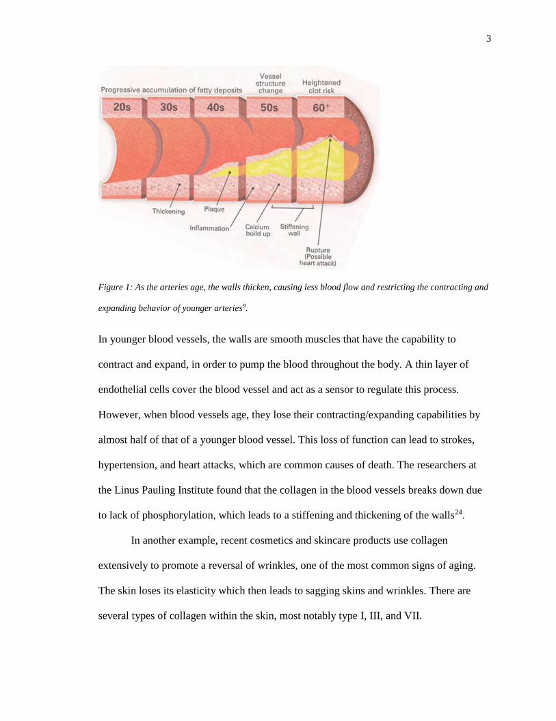
Figure 1: As the arteries age, the walls thicken, causing less blood flow and restricting the contracting and
expanding behavior of younger arteries9.
In younger blood vessels, the walls are smooth muscles that have the capability to
contract and expand, in order to pump the blood throughout the body. A thin layer of
endothelial cells cover the blood vessel and act as a sensor to regulate this process.
However, when blood vessels age, they lose their contracting/expanding capabilities by
almost half of that of a younger blood vessel. This loss of function can lead to strokes,
hypertension, and heart attacks, which are common causes of death. The researchers at
the Linus Pauling Institute found that the collagen in the blood vessels breaks down due
to lack of phosphorylation, which leads to a stiffening and thickening of the walls24.
In another example, recent cosmetics and skincare products use collagen
extensively to promote a reversal of wrinkles, one of the most common signs of aging.
The skin loses its elasticity which then leads to sagging skins and wrinkles. There are
several types of collagen within the skin, most notably type I, III, and VII.
4
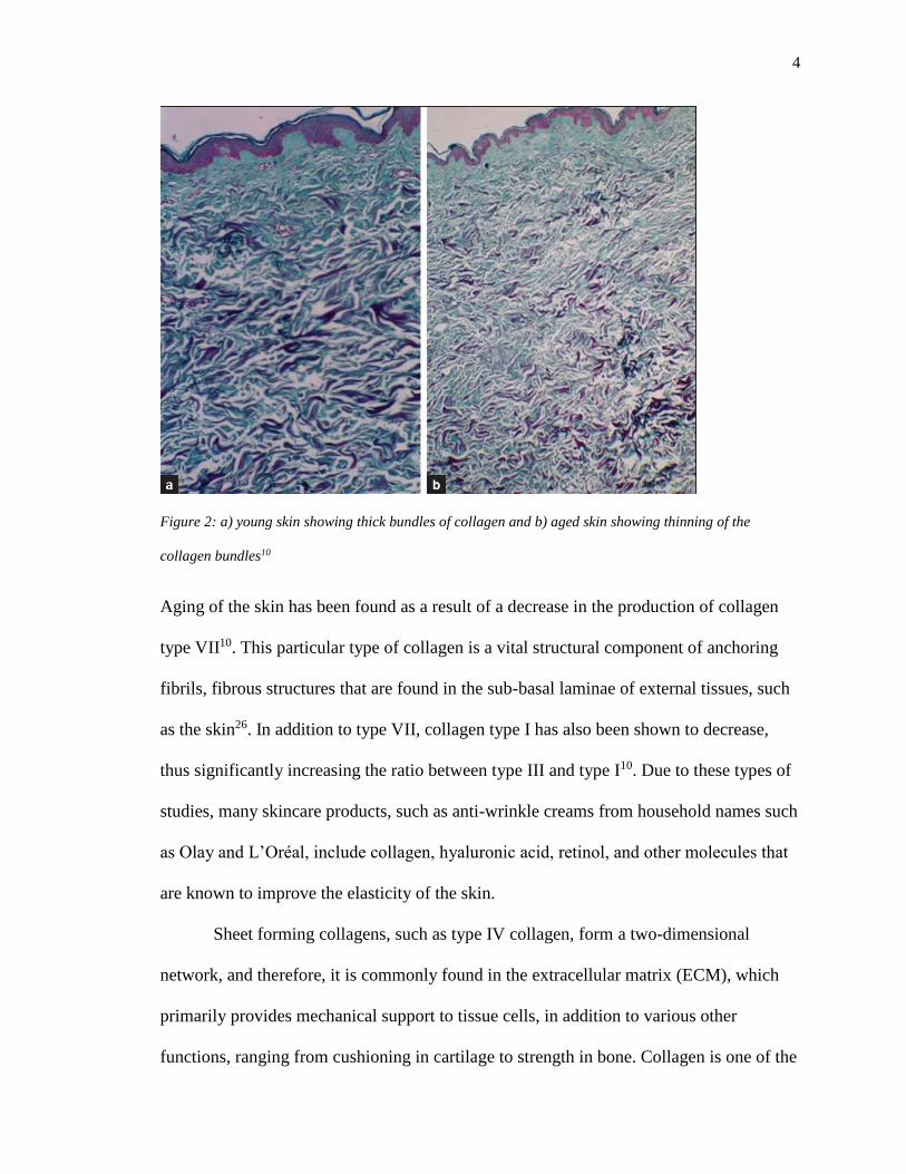
Figure 2: a) young skin showing thick bundles of collagen and b) aged skin showing thinning of the
collagen bundles10
Aging of the skin has been found as a result of a decrease in the production of collagen
type VII10. This particular type of collagen is a vital structural component of anchoring
fibrils, fibrous structures that are found in the sub-basal laminae of external tissues, such
as the skin26. In addition to type VII, collagen type I has also been shown to decrease,
thus significantly increasing the ratio between type III and type I10. Due to these types of
studies, many skincare products, such as anti-wrinkle creams from household names such
as Olay and L’Oréal, include collagen, hyaluronic acid, retinol, and other molecules that
are known to improve the elasticity of the skin.
Sheet forming collagens, such as type IV collagen, form a two-dimensional
network, and therefore, it is commonly found in the extracellular matrix (ECM), which
primarily provides mechanical support to tissue cells, in addition to various other
functions, ranging from cushioning in cartilage to strength in bone. Collagen is one of the

5
three most abundant components of the ECM, along with proteoglycans and soluble
multi-adhesive proteins such as fibronectin. The basal lamina is a special type of ECM,
and primarily separates the connective tissue from the epithelial cells. Type IV and
laminin, a family of multi-adhesive proteins, form their own two-dimensional networks,
which are linked together by entactin molecules, which also helps integrate other
components into the ECM, and perlecan molecules, which are multidomain
proteoglycans that links the ECM components and cell-surface molecules19.
Figure 3: The extracellular matrix is made up of a mesh-like structure of Type IV collagen and laminin,
with entactin and perlecan anchoring the mesh-like structure to different tissues depending on the location
within the body19.
Although the biosynthetic pathway of collagen is complex, there have been extensive
research done to understand the process. The steps are outlined below:
6
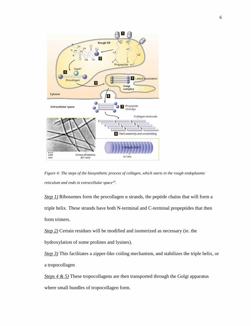
Figure 4: The steps of the biosynthetic process of collagen, which starts in the rough endoplasmic
reticulum and ends in extracellular space19.
Step 1) Ribosomes form the procollagen α strands, the peptide chains that will form a
triple helix. These strands have both N-terminal and C-terminal propeptides that then
form trimers.
Step 2) Certain residues will be modified and isomerized as necessary (ie. the
hydroxylation of some prolines and lysines).
Step 3) This facilitates a zipper-like coiling mechanism, and stabilizes the triple helix, or
a tropocollagen
Steps 4 & 5) These tropocollagens are then transported through the Golgi apparatus
where small bundles of tropocollagen form.

7
Steps 6-8) Once these bundles are in extracellular space, the propeptides are cleaved and
multiple bundles form cross-links in a staggered array, forming a microfibril19.
8
Chapter 2: Background
The abundance of collagen is because of their versatile functionality, primarily
due to their mechanical strength and elasticity. These properties arise from the multiscale
hierarchy of collagen.
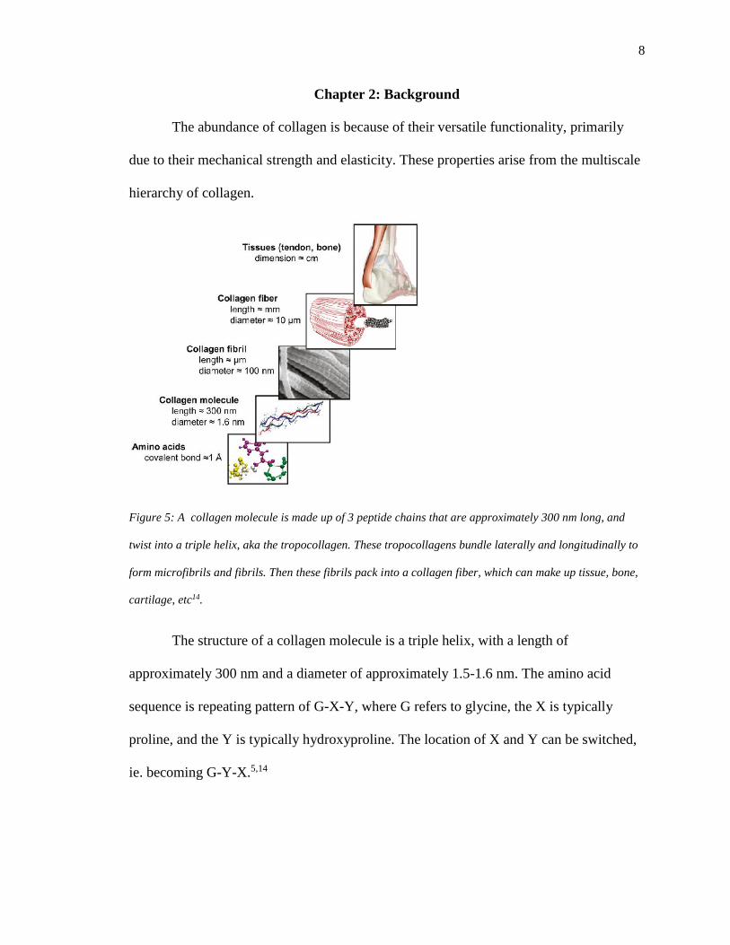
Figure 5: A collagen molecule is made up of 3 peptide chains that are approximately 300 nm long, and
twist into a triple helix, aka the tropocollagen. These tropocollagens bundle laterally and longitudinally to
form microfibrils and fibrils. Then these fibrils pack into a collagen fiber, which can make up tissue, bone,
cartilage, etc14.
The structure of a collagen molecule is a triple helix, with a length of
approximately 300 nm and a diameter of approximately 1.5-1.6 nm. The amino acid
sequence is repeating pattern of G-X-Y, where G refers to glycine, the X is typically
proline, and the Y is typically hydroxyproline. The location of X and Y can be switched,
ie. becoming G-Y-X.5,14
9
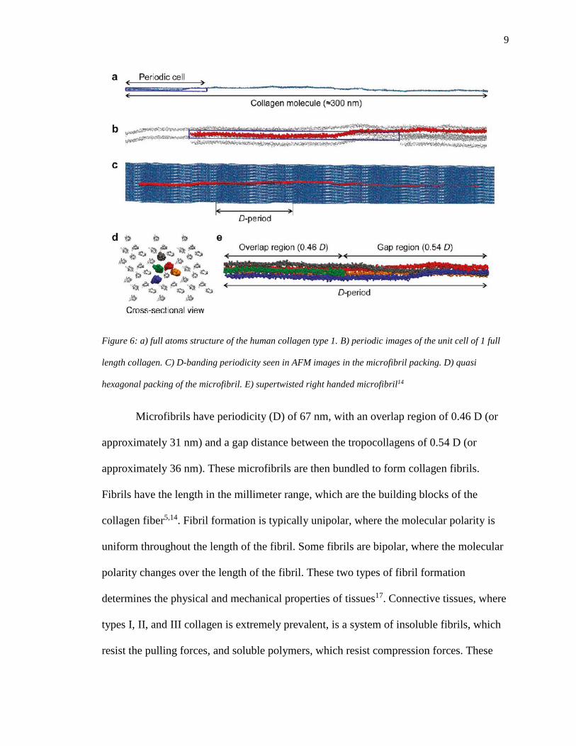
Figure 6: a) full atoms structure of the human collagen type 1. B) periodic images of the unit cell of 1 full
length collagen. C) D-banding periodicity seen in AFM images in the microfibril packing. D) quasi
hexagonal packing of the microfibril. E) supertwisted right handed microfibril14
Microfibrils have periodicity (D) of 67 nm, with an overlap region of 0.46 D (or
approximately 31 nm) and a gap distance between the tropocollagens of 0.54 D (or
approximately 36 nm). These microfibrils are then bundled to form collagen fibrils.
Fibrils have the length in the millimeter range, which are the building blocks of the
collagen fiber5,14. Fibril formation is typically unipolar, where the molecular polarity is
uniform throughout the length of the fibril. Some fibrils are bipolar, where the molecular
polarity changes over the length of the fibril. These two types of fibril formation
determines the physical and mechanical properties of tissues17. Connective tissues, where
types I, II, and III collagen is extremely prevalent, is a system of insoluble fibrils, which
resist the pulling forces, and soluble polymers, which resist compression forces. These
10
molecules aggregate in a “quarter stagger” arrays: 75% of each molecule is in contact
with neighbors next to each other29.
When the structural integrity of collagen is defective, a number of diseases can
arise: Ehlers-Danlos, osteogenesis imperfecta (OI), scurvy, Caffey disease, etc6,28. There
are many different types of collagen, depending on the type of tissue, the form, and the
function, ranging from types I to XI17.
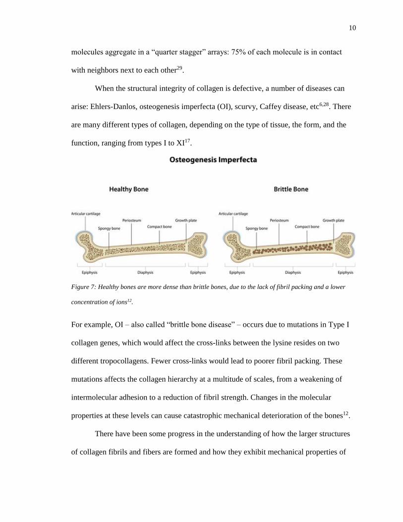
Figure 7: Healthy bones are more dense than brittle bones, due to the lack of fibril packing and a lower
concentration of ions12.
For example, OI – also called “brittle bone disease” – occurs due to mutations in Type I
collagen genes, which would affect the cross-links between the lysine resides on two
different tropocollagens. Fewer cross-links would lead to poorer fibril packing. These
mutations affects the collagen hierarchy at a multitude of scales, from a weakening of
intermolecular adhesion to a reduction of fibril strength. Changes in the molecular
properties at these levels can cause catastrophic mechanical deterioration of the bones12.
There have been some progress in the understanding of how the larger structures
of collagen fibrils and fibers are formed and how they exhibit mechanical properties of

11
strength and stability. Gautieri et al14 validated the experimental data on the mechanical
and elastic properties of a collagen microfibril by using an atomistic simulation.
However, larger scale simulations of fibrils and fibers would get too computationally
expensive. Therefore, the method of coarse-graining would need to be implemented.
Buehler et al5 used atomistic level computer simulations to examine the mechanical and
elastic properties of a full-length collagen molecule in order to create a mesoscopic,
coarse-grained system.
These types of modeling have been primarily steered molecular dynamics (SMD)
in order to test the viscoelasticity of collagen, and calculate the Young’s modulus, a ratio
between tensile stress (𝜎(𝜀)) and strain (𝜀) to calculate the stiffness of a material.
Eq. 1 𝐸 =𝜎(𝜀)
𝜀
Gautieri et al13 found that for collagen, the Young’s modulus ranges from 6 to 16 Gpa.
Ghodsi and Darvish15 also tested the viscoelasticity of a collagen-mimetic microfibril,
composed of two tropocollagens, and found a Young’s modulus of 2.24-3.27 Gpa.
However, much of the focus in these computational studies has not been done on
the mechanism of the triple helix formation and microfibril formation. Some
experimental studies have looked into the kinetics of collagen fibril assembly22, which
have not then been researched in computational studies. This is primarily due to the
complexity of the chemistry surrounding collagen microfibril formation, as well as the
lack of supercomputing power to simulate multiple full length collagen tropocollagens in
a periodic box. With technological advances in supercomputing power, it can be possible
to explore these mechanisms in order to understand the full extent of the collagen

12
hierarchy, which can shed light on how mutations and damage can deform and denature
collagen fibers.
13
Chapter 3: Methodology
3.1 Molecular Dynamics
Computer simulations bridge two different time and length scales, ie. microscopic
and macroscopic. They also bridge theory and experiments; theories can be tested using a
model, which can then be validated with data from experimental studies. There are many
families of simulation techniques that can be utilized in computational studies. Two such
families are Monte Carlo (MC) and molecular dynamics (MD). MC tends to favor gas
and low density systems, whereas MD tends to favor liquid systems and time-dependent
simulations2. For this study, as the tropocollagen molecules will be in an explicit solvent,
MD was chosen because the focus was on the structure and the dynamics of the
tropocollagens and the microfibrils. MC was not chosen because it does not give accurate
structural details or have time significance.
Within MD, there are three main ensembles that can be implemented on a system:
microcanonical, canonical, and isothermal-isobaric. Microcanonical (NVE) ensembles
have a fixed number of molecules, volume, and energy, and corresponds to adiabatic
processes. Canonical (NVT) ensembles differ from NVE in that they do not have a fixed
energy but instead have a fixed temperature. NVT ensembles employ the use of
thermostat algorithms, such as rescaling the velocity, in order to add or remove energy
from the MD simulation boundaries to maintain a constant temperature. Isothermal-
isobaric (NPT) ensembles require a thermostat as well as a barostat since the pressure,
temperature, and number of molecules are fixed1,8.

14
Figure 8: Molecular modeling and it’s application ranges with the approximate time and length scales for
each. This can be expanded into multi-scale schemes18.
However, often times simulating all-atom representations of complex systems,
such as multiple tropocollagens or microfibrils, can get too expensive, even with the
advances in technology. All-atom simulations are primarily limited to small systems and
shorter time scales. As a result, coarse-grained representations reduce the computational
expense and time needed to model various phenomena. Coarse-grained molecular
dynamics (CGMD) simulations can explore larger systems and/or longer time scales.
Well-designed CGMD models can reasonably reproduce the structures of all-atom
simulations, which creates new opportunities to explore multi-scale modeling, combining
the speed of CGMD and the accuracy of all-atom MD18.
In both all-atom or coarse-grained MD, Newton’s equations are solved at every
iteration for each molecule I within the system.
Eq. 2 𝐹𝑖(𝑡) = 𝑚𝑖𝑎𝑖(𝑡)
15
Eq. 3 𝑣𝑖(𝑡) = ∫𝑎𝑖 (𝑡)𝑑𝑡
To solve these equations with discrete time steps, where Δt > 0, the Verlet integration
algorithm is utilized to calculate the trajectories. Within this algorithm, the goal is to
construct a series of positions at each time step using the previous time step’s position.
This does not explicitly calculate velocity. This process is repeated for the duration of the
simulations.
3.2 Molecular Interaction Potentials
These equations can be represented differently, with potential energy (U).
Eq. 4 𝑚𝑖�̈�𝑖 = 𝒇𝑖 where 𝒇𝑖 = −𝜕
𝜕𝒓𝑖𝑈
Potential energy can then be split up into non-bonded and bonded interactions. Non-
bonded interactions can be represented by a sum of N-body interactions.
Eq. 5 𝑈𝑛𝑜𝑛−𝑏𝑜𝑛𝑑𝑒𝑑(𝒓𝑁) = ∑ 𝑢(𝒓𝑖)𝑖 + ∑ ∑ 𝑣(𝒓𝑖, 𝒓𝑗)𝑗>𝑖 +⋯𝑖
The first term is the externally applied potential field, which is dropped for fully periodic
simulations. The second term is the pair potential, and it is common to neglect higher
order interactions (3-body and higher n-body). For complex fluids, it is typically
sufficient to use the simplest models to represent the essential physics and dynamics.
Continuous and differentiable pair-potentials are commonly used, such as Lennard-Jones
and/or Weeks-Chandler-Anderson.
16
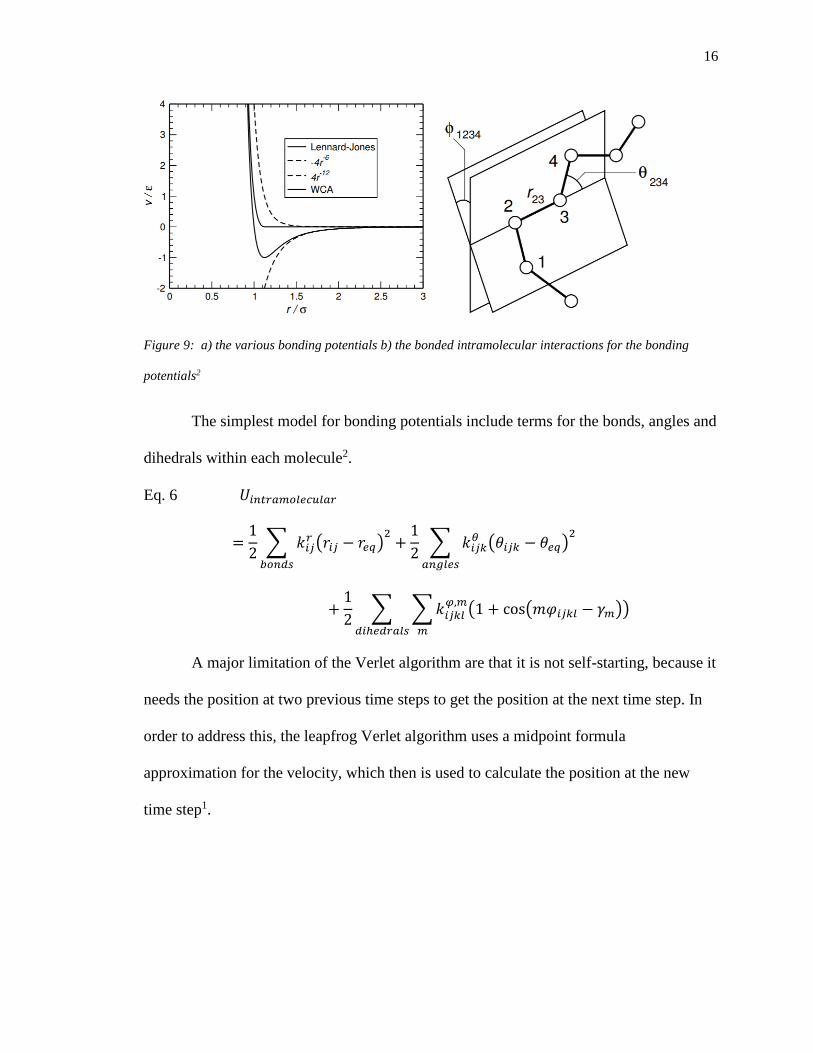
Figure 9: a) the various bonding potentials b) the bonded intramolecular interactions for the bonding
potentials2
The simplest model for bonding potentials include terms for the bonds, angles and
dihedrals within each molecule2.
Eq. 6 𝑈𝑖𝑛𝑡𝑟𝑎𝑚𝑜𝑙𝑒𝑐𝑢𝑙𝑎𝑟
=1
2∑ 𝑘𝑖𝑗
𝑟 (𝑟𝑖𝑗 − 𝑟𝑒𝑞)2
𝑏𝑜𝑛𝑑𝑠
+1
2∑ 𝑘𝑖𝑗𝑘
𝜃 (𝜃𝑖𝑗𝑘 − 𝜃𝑒𝑞)2
𝑎𝑛𝑔𝑙𝑒𝑠
+1
2∑ ∑𝑘𝑖𝑗𝑘𝑙
𝜑,𝑚(1 + cos(𝑚𝜑𝑖𝑗𝑘𝑙 − 𝛾𝑚))
𝑚𝑑𝑖ℎ𝑒𝑑𝑟𝑎𝑙𝑠
A major limitation of the Verlet algorithm are that it is not self-starting, because it
needs the position at two previous time steps to get the position at the next time step. In
order to address this, the leapfrog Verlet algorithm uses a midpoint formula
approximation for the velocity, which then is used to calculate the position at the new
time step1.

17
3.3 Protein Models
There are many different CGMD models for protein simulations, with a wide
variety of applications, ranging from protein folding mechanisms to protein structure
predictions to protein-protein recognition.
Coarse-grained
Model
Acronym/Name
Acronym’s
Meaning
Model Design Example Applications
AWSEM Associated
memory,
Water
mediated,
Structure and
Energy
Model
Up to 3 bead
representation: Cα,
Cβ, and O.
Ab initio structure
preditction of globular
proteins; modeling the
mechanisms of misfolding
and aggregation
Bereau and
Deresno
-- Up to 4 bead
representation: 3
backbone beads (N,
Cα and C’) and 1
side chain bead at
Cβ
Studying protein folding
and aggregation
CABS C-Alpha, C-
Beta, Side
chain
Up to 4 bead
representation: Cα,
Cβ, center of the
side chain, and
center of the peptide
bond.
Ab initio protein structure
prediction; ab initio
simulations of protein
folding
MARTINI -- Up to 5 bead
representation: 1
backbone bead and
up to 4 side chain
beads
Originally for lipids and has
expanded for proteins. Most
popular for coarse-grained
modeling of membrane
proteins in the membrane
environment
OPEP Optimized
Potential for
Efficient
protein
Up to 6 bead
representation: full
atom for backbone
(N, HN, Cα, C’, O)
and 1 bead for side
Modeling of proteins,
DNA-RNA complexes and
amyloid fibril formation;
structure prediction of
peptides and small proteins

18
structure
Prediction
chains (sans PRO
with 3 beads)
PaLaCe Pasi-Lavery-
Ceres
2-tier representation
– 1 for bonded and 1
for non-bonded
interactions
Modeling dynamic
fluctuations of folded
proteins; protein flexibility
prediction
PRIMO -- Up to 7 bead
representation: 3
backbone beads (N,
Cα, CO) and 1 to 5
side chain beads
Modeling peptide and small
protein structure prediction;
been expanded to
membrane environments
Rosetta -- Representation by
all backbone atoms,
Cβ, and center of
side chain.
Widely used for protein
structure prediction
SCORPION Solvated
Coarse-
grained
Protein
Interaction
Up to 3 bead
representation: 1
backbone bead and
1 to 2 side chain
beads
Initially for scoring protein-
protein complexes; later
used for protein-protein
recognition in a solvated
environment
UNRES United
Residue
3 bead
representation: Cα,
peptide group and
side chain
Modeling loop structure
prediction; protein-DNA
interactions; large-scale
rearrangements of protein
complexes Table 2: Select coarse grain protein models, with their model design and some applications18.
The UNRES model is the most classical model of intermediate resolution, with a
dependable and a quick reconstruction of the all-atom representation. CABS is another
model of intermediate resolution, similar to UNRES, but it differs in its interactions and
sampling concepts. PRIMO has a higher resolution than CABS or UNRES, which makes
it closer to all-atom representation. The MARTINI model’s mapping scheme provides an
effective and straightforward method of switching between all-atom and coarse-grained
representations, with a plethora of biological applications. The Rosetta model has 2

19
protein representations: the all-atom and the coarse-grained, combined with the presence
of all of the hydrogen atoms. This allows the model to define a confirmation of a protein
in with respect to the dihedral space. This is a versatile model for resolution as the
program can switch between low and high resolution for a system18.
Figure 10: Comparing all-atom and coarse-grained modeling for aggregation processes. The “Under
construction” region refers to the current inability of mapping the intermediate aggregation stages to all-
atom modeling18.
Despite the gains made within protein modeling and the mapping that occurs
between all-atom and coarse-grained representations, there is still some areas that can be
explored. The opportunity to use coarse-grained models to describe aggregation at larger
length scales and longer time scales goes beyond the limitations of atomistic
simulations18. Collagen is one such target for these types of coarse-grained models.
Gautieri, Buehler, and their colleagues have started the aggregation process of collagen
20
peptides into tropocollagens and some microfibril formation. However, mapping the
microfibril to fibril networks has not yet been explored, a gateway into understanding the
formation of gels from fibrils.
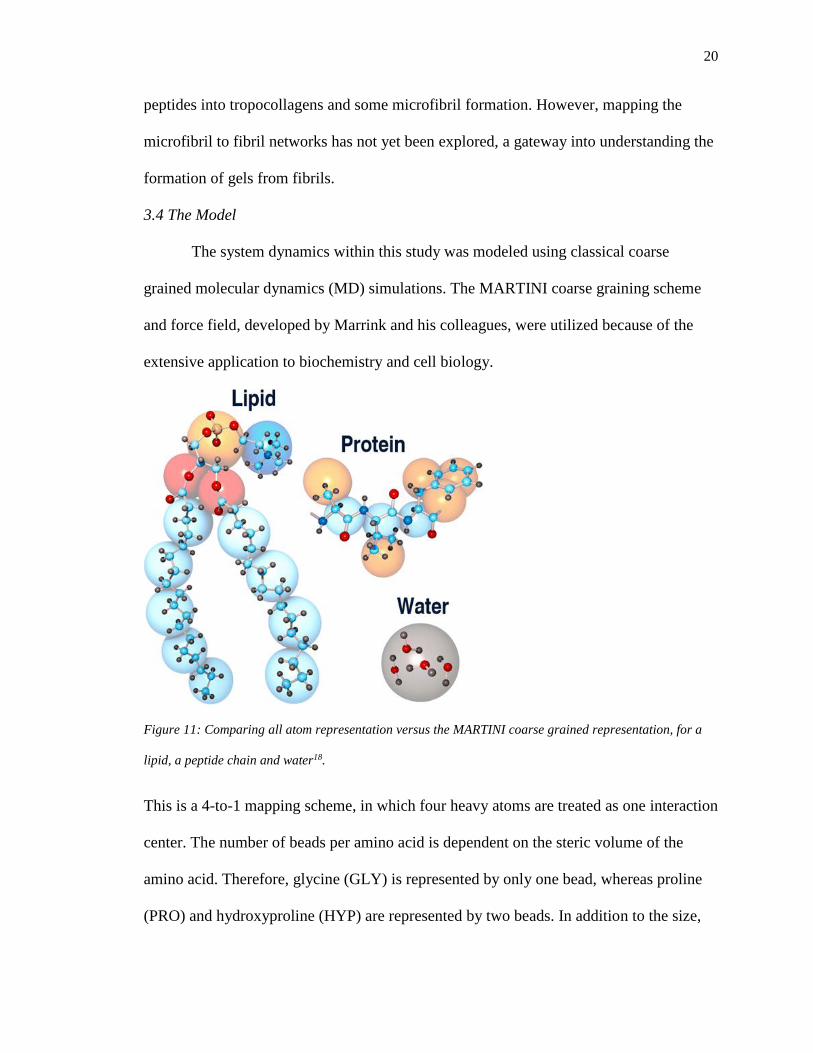
3.4 The Model
The system dynamics within this study was modeled using classical coarse
grained molecular dynamics (MD) simulations. The MARTINI coarse graining scheme
and force field, developed by Marrink and his colleagues, were utilized because of the
extensive application to biochemistry and cell biology.
Figure 11: Comparing all atom representation versus the MARTINI coarse grained representation, for a
lipid, a peptide chain and water18.
This is a 4-to-1 mapping scheme, in which four heavy atoms are treated as one interaction
center. The number of beads per amino acid is dependent on the steric volume of the
amino acid. Therefore, glycine (GLY) is represented by only one bead, whereas proline
(PRO) and hydroxyproline (HYP) are represented by two beads. In addition to the size,

21
there are four types of interactions: polar, nonpolar, apolar, and charged. Within each
type, subtypes are distinguished by hydrogen bonding capabilities (donor, acceptor, both,
none) and degree of polarity (from 1 as the lowest polarity to 5 as the highest polarity).
As a result, an amino acid’s specific chemistry is retained.
Figure 12: MARTINI mapping for all 20 amino acids, where the names are in the three letter code21.
Non-bonded interactions of particle pairs I and j at a distance rij are modeled via
the (12, 6) Lennard-Jones (LJ) potential.
Eq. 7 𝑉𝐿𝐽(𝑟𝑖𝑗) = 4𝜀𝑖𝑗[(𝜎𝑖𝑗
𝑟𝑖𝑗)12 − (
𝜎𝑖𝑗
𝑟𝑖𝑗)6]
The strength of the interactions are based on the depth of the attractive well, governed by
the parameter ε. Charged groups not only interact via the Lennard-Jones potential, but
also via a Coulombic energy function.
Eq. 8 𝑉𝐶𝑜𝑢𝑙𝑜𝑚𝑏 =𝑞𝑖𝑞𝑗
4𝜋𝜀0𝜀𝑟𝑒𝑙𝑟𝑖𝑗

22
Bonded interactions between bonded sites I, j, k, and l are described by a set of harmonic
potential energy functions for the deformations of the bond length, angles, and
dihedrals20.
Eq. 9 𝑉𝑏𝑜𝑛𝑑 =1
2𝐾𝑏𝑜𝑛𝑑(𝑑𝑖𝑗 − 𝑑𝑏𝑜𝑛𝑑)
2
Eq. 10 𝑉𝑎𝑛𝑔𝑙𝑒 =1
2𝐾𝑎𝑛𝑔𝑙𝑒[cos(𝜑𝑖𝑗𝑘) − cos(𝜑𝑎𝑛𝑔𝑙𝑒)]
2
Eq. 11 𝑉𝑑𝑖ℎ𝑒𝑑𝑟𝑎𝑙 = 𝐾𝑑𝑖ℎ𝑒𝑑𝑟𝑎𝑙[1 + cos(𝑛𝜓𝑖𝑗𝑘𝑙 − 𝜓𝑑𝑖ℎ𝑒𝑑𝑟𝑎𝑙)]
The interactions between the different bead types is based on the well depth (ε) of
the LJ potential: IX=2.0 kJ/mol, VIII=2.0 kJ/mol, VII=2.3 kJ/mol, VI=2.7 kJ/mol, V=3.1
kJ/mol, IV=3.5 kJ/mol, III=4.0 kJ/mol, II=4.5 kJ/mol, I=5.0 kJ/mol, O=5.6 kJ/mol.
Q P N C
Sub Da d a 0 5 4 3 2 1 da d a 0 5 4 3 2 1
Q Da O O O II O O O I I I I I IV V VI VII IX IX
D O I O II O O O I I I III I IV V VI VII IX IX
A O O I II O O O I I I I III IV V VI VII IX IX
0 II II II IV I O I II III III III III IV V VI VII IX IX
P 5 O O O I O O O O O I I I IV V VI VI VII VIII
4 O O O O O I I II II III III III IV V VI VI VII VIII
3 O O O I O I I II II II II II IV IV V V VI VII
2 I I I II O II II II II II II II III IV IV V VI VII
1 I I I III O II II II II II II II II IV IV IV V VI
N Da I I I III I III II II II II II II IV IV V VI VI VI
D I III I III I III II II II II III II IV IV V VI VI VI
A I I III III I III II II II II II III IV IV V VI VI VI
0 IV IV IV IV IV IV IV III IV IV IV IV IV IV IV IV V VI
C 5 V V V V V V IV IV IV IV IV IV IV IV IV IV V V
4 VI VI VI VI VI VI V IV V V V V IV IV IV IV V V
3 VII VII VII VII VI VI V V VI VI VI VI IV IV IV IV IV IV
2 IX IX IX IX VII VII VI VI VI VI VI VI V V V IV IV IV
1 IX IX IX IX VIII VIII VII VII VI VI VI VI VI V V IV IV IV
Table 3: Interaction matrix between all bead subtypes20.

23
In its extension to proteins, Monticelli et al21 set basic parametrization for bond
length, angles, dihedrals, force constants, etc. Gautieri et al11 applied the MARTINI
model to collagen amino acids, and characterized HYP according to the mapping and its
corresponding parameters. For this study, the tripeptide periodic sequence consists of
GLY, PRO, and HYP, based on the characterization by Gautieri et al, with a few changes.
Amino Acid Backbone
bead type
Side chain
bead type
GLY N0* --
PRO C5 C2**
HYP C5 P1 Table 4: *In Monticelli et al21, for GLY in helices, the BB bead type was modified to N0 from C5 to account
for the properties of a helix. **In MARTINI version 2.0, this was AC2, which is used by Gautieri et al11, but
from version 2.1 this was C2.
𝑑𝑏𝑜𝑛𝑑 [nm]
𝐾𝑏𝑜𝑛𝑑 [kJ mol-1 nm-2]
𝜑𝑎𝑛𝑔𝑙𝑒
[deg]
𝐾𝑎𝑛𝑔𝑙𝑒
[KJ mol-1]±
𝜓𝑑𝑖ℎ𝑒𝑑𝑟𝑎𝑙 [deg]**
𝐾𝑑𝑖ℎ𝑒𝑑𝑟𝑎𝑙 [KJ mol-1]**
BB-BB 0.365 100* 98** 1250 60 400
BB-SC 0.300 7500 100 1250 60 400 Table 5: *Decreased this force constant from the reported value of 200 for a coil by Monticelli et al21 to
introduce more flexibility of the triple helical formation and then the coiling of the tropocollagens in the
microfibril formation. ** this were the reported values for a helix. ±Increased this force constant from the
reported value of 700 for a helix by Monticelli et al21 to introduce more rigidity of the PRO and HYP side
chain beads for the microfibril formation.
The major changes from the previous works for these parameters occur with the
backbone to backbone force constants. The force constant of the bond was decreased in
order to facilitate more flexibility of the assembled tropocollagen for the microfibril
formation. Tropocollagens form a right handed coil when assembling into a microfibril.
The added flexibility was added to ensure that the triple helix does not undo when coiling
into a microfibril27. The force constant of the angle was increased in order to increase the

24
rigidity of the angle and maintain an average distance of 0.5 nm between the PRO and
HYP side chain beads4. Using these values, we created a Martini coarse grained
simplified collagen molecule of only [GLY-PRO-HYP]27 repeats.
Figure 13: 1 peptide strand that consists of [GLY-PRO-HYP]9 where GLY is in green, PRO is in yellow,
and HYP is in magenta
This amounts to 45 MARTINI coarse grained beads for one peptide strand. All of the
simulations were run using Groningen Machine for Chemical Simulations (GROMACS),
an MD package intended for the simulations of cellular level biology – primarily
proteins, lipids, and nucleic acids. GROMACS was originally started at the Department
of Biophysical Chemistry at the University of Groningen in the Netherlands. Its goal was
to create a parallel computer system specifically for molecular simulations. This
particular package was selected because of it is extremely fast at calculating non-bonded
interactions, which tend to dominate simulations, It can run on central processing units
(CPUs) and graphics processing units (GPUs), allowing for a wider application of the
software package without compromising accuracy and speed. The speed varies from 3 to

25
10 times faster than many other simulation programs. GROMACS’s ability to be
executed in parallel is another reason why this particular software package was chosen. In
addition, the data output files can easily be viewed in software packages such as Visual
Molecular Dynamics (VMD), which was used for this particular study16.

26
Chapter 4: Triple Helix Simulations
A MATLAB code was created based on the MARTINI coarse-grained mapping
of the various amino acids, including HYP. This code wrote the input files of one [GLY-
PRO-HYP]27 peptide strand, based on an input sequence. As a result, future studies that
change the sequence can still utilize this code. This one peptide strand was then simulated
using the MARTINI force field version 2.2. The system was equilibrated, using the
steepest descent algorithm, for about 1 ns with a time step of 1 fs in an extremely large
periodic box (30x30x30 nm3), to ensure a stable structure. This particular equilibration
occurred without any water molecules because one of the goals was to ensure that the
input parameters did not cause the simulation to blow up. The other goal was to measure
the length of the peptide strand, for the next simulations. With a large periodic box, the
inclusion of water molecules will greatly slow down the computational speed. In
addition, the presence of only one peptide strand in water would not yield any significant
results for this particular study. In addition, the time step is fairly small to track to the
changes in the potential energy as the
The total length of the peptide strand was found to be approximately 6.9 nm. This
length is particularly useful in calculating the size of the periodic box for the
tropocollagen simulations. A common guideline for computer simulations is to have a
periodic box size that is about 1.5 times larger than the length of the molecule. This is to
ensure that one end of the molecule does not interact with its other end through the
periodic boundary walls. As a result, the tropocollagen simulations had a periodic box
size of 11x11x11 nm3. Then the one peptide strand was replicated two more times, to
have a total of 3 peptide strands, with a total of 135 MARTINI coarse-grained beads,

27
placed randomly within the periodic box. Once this was solvated with water and positive
ions, there were approximately 10,600 water beads and enough positive ions to ensure
that the charge of the system is neutral.
Figure 14: A zoomed-in view of the 3 peptide strands in solvent, where GLY is green, PRO is yellow, HYP
is magenta.
Sodium ions were chosen due to the polarity of the HYP beads and the
interactions between them and the water beads. The energy of this system was minimized
for 1 ns with a time step of 1 fs, similar to how the energy of the 1 peptide strand was
minimized earlier. Then, the Molecular Dynamics simulation ran for 320 ns with a time
step of 8 fs. Typically, the time steps for coarse-grained molecular simulations are around
20 to 30 fs. However, with the presence of dihedrals, the time step is often around 10 fs,
due to the extra constraints that dihedrals present to the calculations.
The MD simulation was done in the GROMACS package using the standard
integrator, a leap-frog algorithm for integrating Newton’s equations of motion16. This
system operates at NVT, with the temperature at 310 K, which is approximately 37°C or

28
the average body temperature. The temperature coupling for the themostat was done
using velocity rescaling, which is similar to the Berendsen thermostat. This allows for
random seeds to be set manually. The Parrinello-Rahman barostat was also applied, in
order to keep the temperature constant20.
Figure 15: After 120 ns, the tropocollagen appears to have formed a complete triple helix. It is unclear at
this point of the simulation whether it is stable.
After 120 ns are completed in the simulation, the tropocollagen is in a complete triple
helix-like configuration. The completeness refers to the three strands being twisted
around throughout the length of the tropocollagen. To test the stability of this
tropocollagen, the system was simulated for another 200 ns. Within these 200 ns, the
29
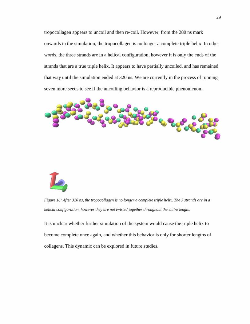
tropocollagen appears to uncoil and then re-coil. However, from the 280 ns mark
onwards in the simulation, the tropocollagen is no longer a complete triple helix. In other
words, the three strands are in a helical configuration, however it is only the ends of the
strands that are a true triple helix. It appears to have partially uncoiled, and has remained
that way until the simulation ended at 320 ns. We are currently in the process of running
seven more seeds to see if the uncoiling behavior is a reproducible phenomenon.
Figure 16: After 320 ns, the tropocollagen is no longer a complete triple helix. The 3 strands are in a
helical configuration, however they are not twisted together throughout the entire length.
It is unclear whether further simulation of the system would cause the triple helix to
become complete once again, and whether this behavior is only for shorter lengths of
collagens. This dynamic can be explored in future studies.

30
Chapter 5: Microfibril Simulations
Once a stable triple helix was formed, it was then replicated five more times, to
get a total of six triple helices or 18 peptide strands. With the increase of strands, the
periodic box size was increased to 20x20x20 nm3, resulting in ~63000 water beads and a
corresponding increase in positive ions.
Figure 17: The initial configuration of the 6 tropocollagens within the periodic box.
These strands were then simulated for approximately 1.1 μs, using the same MD
simulation parameters as before with the tropocollagen simulations. The increase in
simulation time is because of the larger number of particles. For the tropocollagen
simulation, there were only approximately 10,600 particles in total. For the microfibril
31
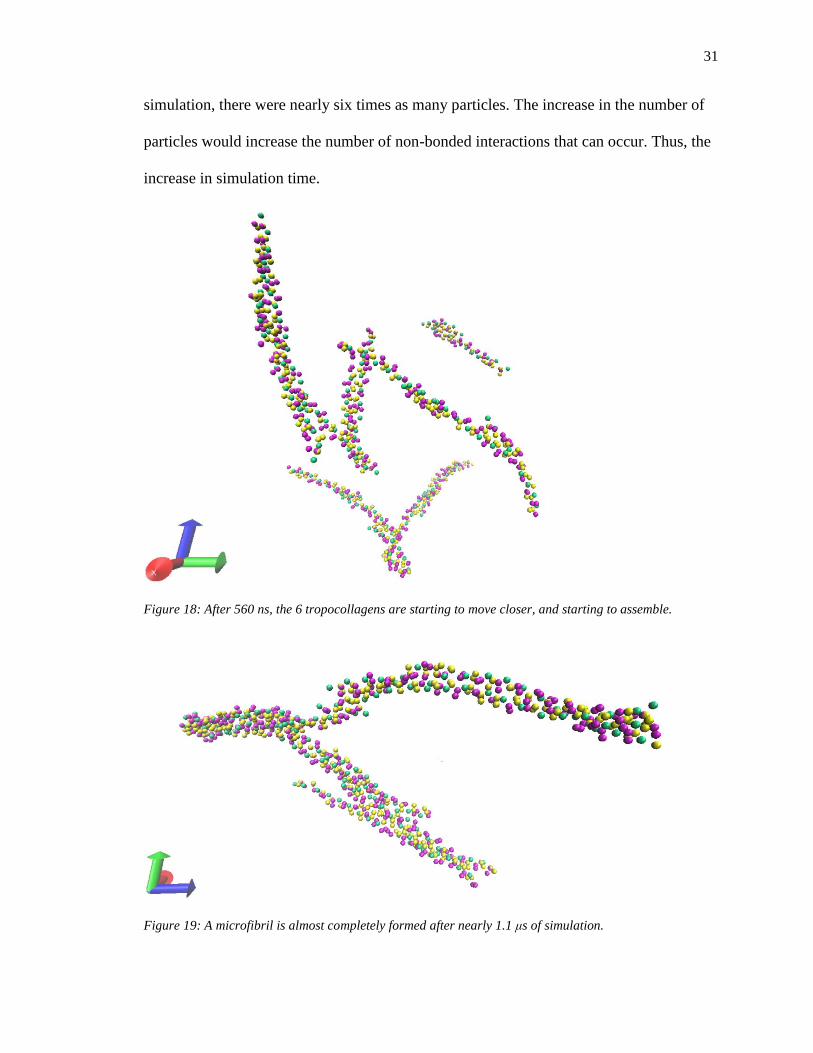
simulation, there were nearly six times as many particles. The increase in the number of
particles would increase the number of non-bonded interactions that can occur. Thus, the
increase in simulation time.
Figure 18: After 560 ns, the 6 tropocollagens are starting to move closer, and starting to assemble.
Figure 19: A microfibril is almost completely formed after nearly 1.1 μs of simulation.

32
After nearly 1.1 μs of simulation, an almost complete microfibril-like bundle is formed. It
spans nearly the entire periodic box’s diagonal, and the strands appear to twist around
each other. It is unclear at this point whether those strands are forming tropocollagens
and then those tropocollagens are forming a microfibril, or the strands are all twisting
around each other to form a microfibril-like structure. Future studies may be able to
characterize the structures formed to determine the correct mechanism of the assembly.

33
Chapter 6: Results & Discussion
6.1 Helicity of the Triple Helix
First, we had to ensure that the tropocollagen is indeed a triple helix, or at least in
some sort of helical configuration. Based on the VMD images, it qualitatively seems to
be a triple helix, especially when it is fully twisted. Even when it is partially uncoiled, it
still appears to be in a helical configuration. However, the characteristics of a helix can
be quantified. The tilt of each of the strands within the triple helix was calculated, using
the Nonlinear Regression Analysis Program (NLREG) demonstration code provided by
Phillip H. Sherrod. NLREG works by taking the data and attempting to find the curve of
best fit for the data provided. In order to do so for a 3-dimensional molecule, the data had
to be independent of one of the 3 directions (x, y, z). This is done by setting one direction
equal to zero (ie. z=0)23.

34
Figure 20: For a collagen helix, the mean angle (θ) is approximately 57°, and δ is the disorder width, or
the range in which the angle could reside. Therefore, the range is between 23° and 90° for a collagen
helix30.
The regression was done for each strand each of the three directions, by setting x=0, then
y=0, then z=0, to figure out which 2-dimensional projection would work best with the
data. Therefore 9 different regressions were performed, and it was found that a projection
on the XY plane worked best for this particular tropocollagen.

35
These angles fall within the range of angles for a collagen helix (23° to 90°),
based on experimental data30. This characterization is not enough to show that a stable
triple helix has been achieved. To further quantify the tropocollagen, we went back to the
literature. A collagen triple helix has an axial rise of 2.86 nm, a diameter of
approximately 1.5 nm, with the PRO ring on one strand and the HYP ring on another
strand being about 0.5 nm apart. Notably, collagen can either be in a “relaxed” triple
helix or a “rigid” triple helix. The “relaxed” form is the 10/3 (10 amino acids per 3 turns)
and the “rigid” form is the 7/2 (7 amino acids per 2 turns)4.
Strand 1 (green) 87.9790°
Strand 2 (red) 26.5993°
Strand 3 (blue) 55.6253°
Figure 21: Schematic of the angles calculated for the 3 peptide strands. The table shows the calculated
angles from the NLREG code.
θ2
θ1
θ3
+z

36
Figure 22: A collagen triple helix parameters, where the axial rise is 2.86 nm and the distance between the
PRO ring and the HYP ring is 0.5 nm4.
In addition, a helix can be mathematically represented by a set of three parametric
equations.
Eq. 12 𝑥 = 𝑟𝑐𝑜𝑠(𝑡)
Eq. 13 𝑦 = 𝑟𝑠𝑖𝑛(𝑡)
Eq. 14 𝑧 = 𝑐𝑡 = (𝑎𝑥𝑖𝑎𝑙𝑟𝑖𝑠𝑒
2𝜋)𝑡
For the reported values of a collagen triple helix, these parametric equations then
become:
Eq. 15 𝑥 = (0.75)𝑐𝑜𝑠(𝑡)
Eq. 16 𝑦 = (0.75)𝑠𝑖𝑛(𝑡)
Eq. 17 𝑧 = (0.4551)𝑡

37
Based on these equations, it is possible to calculate the curvature (κ) and torsion (τ) of a
helix. Curvature is the rate of change of a unit vector along the direction of motion along
the curve. Essentially, it is the rate at which a curve bends. The radius of curvature is 1/ κ.
Torsion is the magnitude of the rate at which a curve twists around an axis3,7.
Mathematically for a helix, they can be expressed like this:
Eq. 18 κ =𝑟
(𝑟2+𝑐2)
Eq. 19 τ =𝑐
(𝑟2+𝑐2)
For the collagen triple helix, κ = 0.9744 and τ = 0.5914. In order to calculate the
curvature and torsion for the simulated tropocollagen, the coordinates were found using
VMD and an approximate axial rise and diameter were calculated. For this simulated
tropocollagen, the approximate diameter is 1.55 nm and the approximate axial rise is 3.18
nm. Therefore, the κ = 0.9237 and τ = 0.6395. The approximate axial rise is slightly off
from the reported value of 2.86 nm, however, there have been some discrepancies
regarding this value. Experimental studies have shown that different types of collagen
have different values for the axial rise. This arises from the fact that the amino acid
sequence for collagen is not merely a repeating tripeptide of GLY-PRO-HYP. There is
much variability, with some collagen types having regions with multiple axial rises along
the same tropocollagen25. The curvature is approximately the same, however the torsion
is noticeably different. This result may be due to the short length of the tropocollagen,
which may not be long enough for the strands to twist tightly around the axis, so the
torsion is higher.
Next, we checked the distance between the side chain beads of a PRO residue that
of a HYP residue on one strand. Similar to the curvature and torsion, the coordinates of

38
the side chain beads were found using VMD, and a simple 3-dimensional distance
formula was applied.
Eq. 20 𝑑 = √((𝑥𝑃𝑅𝑂 − 𝑥𝐻𝑌𝑃)2 + (𝑦𝑃𝑅𝑂 − 𝑦𝐻𝑌𝑃)2 + (𝑧𝑃𝑅𝑂 − 𝑧𝐻𝑌𝑃)2)2
For this simulated tropocollagen, the distance was approximately 0.55 ± 0.08 nm, which
is close to the reported value of 0.5 nm4. This indicates that the hypothesis of increasing
the force constant of the angle in order to achieve the reported value between the PRO
and HYP side chain beads is correct. This can be further optimized in future studies.
6.2 Interaction Counts
To find out whether or not the collagen triple helix did uncoil after 320 ns, we
calculated the interaction counts. For this study, an interaction count is when two beads
on different strands are within the LJ cutoff of 1.2 nm. Any distance less than the cutoff
would result in the two beads interacting following the LJ potential, whereas any distance
greater than the cutoff would result in the two beads not interacting at all. The
calculations were done by creating a MATLAB code that reads the positions of each of
the beads on one strand, and then finds the distance to the beads on the other strands. In
order to figure out if the various strands are interacting, the distance was checked against
the cutoff. The interactions for the triple helix would occur between strands 1 and 2, 2
and 3, and 3 and 1, resulting in three separate interaction counts. An average was taken
over time to find out the average interaction count for each strand pair.

39
Figure 23: The average number of interactions between the strand pairs. The highest consistently occurs
between strand 2 and 3. On the other hand, strand 1 is minimally interacting with either strand 2 or strand
3.
For the triple helix, strands 3 and 2 had the highest average interaction count throughout
the simulation, with approximately sixteen interaction counts. This corresponds to the
parallel orientation of these two strands, as shown by figure 16. Therefore, these two
strands are interacting throughout the length of the strand. Strand 1 minimally interacts
with the other two strands, as shown by figure 16. This strand is only interacting with the
other two at the ends, which is why the average interaction count is approximately two.
These results can lead to the conclusion that the triple helix has partially uncoiled.
The same logic was then applied to the microfibril system. The code was
modified for this system so that it would count the interaction between strand 1 and
strands 2-18, etc. This results in eighteen different average interaction counts over the
duration of the simulation.
0
2
4
6
8
10
12
14
16
Aver
age
Num
ber
of
Inte
ract
ions
bet
wee
n p
airs
Strands 2 to 1 Strands 3 to 2 Strands 1 to 3

40
Figure 24: The average interaction counts for each of the 18 interactions. Each bar in the histogram refers
to the strand to which the pairs were taken -- ie. Strand 1 implies the interactions between sstrands2 to 1, 3
to 1, etc.
A similar pattern appears for the microfibril system as compared to the tropocollagen
system. Strand 17 has the fewest interactions with the others, and strand 1 has the second
fewest. The strands with less than eight interactions with the other strands are 3, 5, 7, 9,
11, 13, 14, 15, 16, and 18. The strands with more than eight interactions are 2, 4, 6, 8, 10,
and 12. These two groups have less than the maximum average interaction counts from
the tropocollagen system of fifteen.
0
1
2
3
4
5
6
7
8
9
10
11
Aver
age
Num
ber
of
Inte
ract
ions
per
Str
and
Strand 1 Strand 2 Strand 3 Strand 4 Strand 5 Strand 6
Strand 7 Strand 8 Strand 9 Strand 10 Strand 11 Strand 12
Strand 13 Strand 14 Strand 15 Strand 16 Strand 17 Strand 18
41
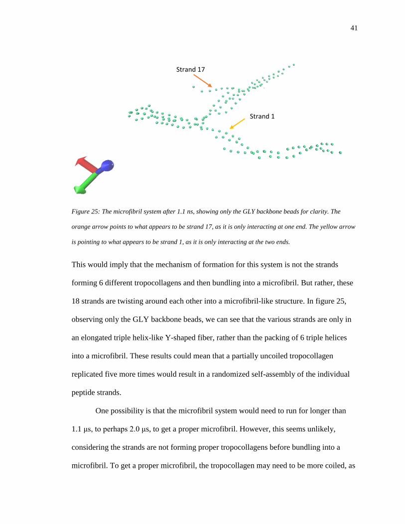
Figure 25: The microfibril system after 1.1 ns, showing only the GLY backbone beads for clarity. The
orange arrow points to what appears to be strand 17, as it is only interacting at one end. The yellow arrow
is pointing to what appears to be strand 1, as it is only interacting at the two ends.
This would imply that the mechanism of formation for this system is not the strands
forming 6 different tropocollagens and then bundling into a microfibril. But rather, these
18 strands are twisting around each other into a microfibril-like structure. In figure 25,
observing only the GLY backbone beads, we can see that the various strands are only in
an elongated triple helix-like Y-shaped fiber, rather than the packing of 6 triple helices
into a microfibril. These results could mean that a partially uncoiled tropocollagen
replicated five more times would result in a randomized self-assembly of the individual
peptide strands.
One possibility is that the microfibril system would need to run for longer than
1.1 μs, to perhaps 2.0 μs, to get a proper microfibril. However, this seems unlikely,
considering the strands are not forming proper tropocollagens before bundling into a
microfibril. To get a proper microfibril, the tropocollagen may need to be more coiled, as
Strand 17
Strand 1
42
it appeared to be in about 120 ns into the first simulation. This process would need to be
further optimized in future studies, in order to form a stable tropocollagen that does not
coil, even partially, and to form the microfibril. One such optimization method could be
to utilize SMD in order to force the tropocollagens to form a microfibril. This may be
closer to the biological pathway of collagen formation, as various “helper” molecules,
ribosomes, enzymes, and even the propeptides at the ends of the collagen peptide strands
aid in the formation of triple helices and fibrils. We are currently in the process of
simulating this microfibril system up to 2.0 μs, as well as running seven more seeds to
determine if this mechanism is a reoccurring phenomenon.
43
Chapter 7: Conclusions
In this study, we have simulated three strands made up of [GLY-PRO-HYP]27 in
order to form a triple helix-like structure. This structure was then characterized using the
parametric equations for a helix, with a curvature κ = 0.9237 and a torsion τ = 0.6395,
which are extremely similar to the ones calculated using the reported values of a collagen
triple helix. We also calculated the distance between the PRO side chain beads on one
strand with the HYP side chain beads on another strand. The distance was found to be
0.55 nm, which is extremely similar to the reported 0.5 nm value for a collagen triple
helix. Therefore, we were able to characterize the triple helix using mathematical
equations. However, the triple helix appeared to have partially uncoiled.
Then, we went on to calculate the interaction count by comparing the distance
between beads on different strands with the LJ cutoff value of 1.2 nm. When we
calculated the average interaction counts between the strands for the triple helix, we
found that only strands 2 and 3 had interactions throughout the length of the strand. The
corresponds to the VMD image of the tropocollagen at 320 ns, where these two strands
appear to be twisting around each other and strand 1 is interacting with them at the ends.
A similar story appeared for the microfibril system, where strand 1 and 17 had the fewest
interactions, a result that corresponded to the VMD image. Therefore, it appears that the
individual strands are bundling to form a microfibril-like structure, or an elongated triple
helix-like structure. It appears to not form a properly coiled tropocollagen, with a more
stable triple helix. It is unclear whether or not this is due to the length of the strands.
Future studies can explore this by simulating a much longer peptide strand, around 50
residues, in order to see if the same sort of coiling and bundling mechanism occurs.

44
Chapter 8: Future Work
Future studies can optimize the results found in this study, by lengthening the
peptide strand, tuning the force parameters, utilizing SMD, etc. Once the interactions are
better understood within a microfibril, this MARTINI coarse grained scheme can be
mapped to an “ultra-coarse grained” scheme that can simulate hundreds of tropocollagens
to form gels and much larger networks. A larger scale could also explore the mechanisms
of deterioration of the collagen fibers.

45
Bibliography
1. Allen, M.P.; Tildesley, D.J. Computer Simulation of Liquids; Clarendon Press:
Oxford, 1989.
2. Attig, Norbert; Binder Kurt; Grumüller, Helmut; Kremer, Kurt (Eds). Computational
Soft Matter: from Synthetic Polymers to Proteins; NIC-Directors: Jülich, Germany,
2004.
3. Bahrami, Amir Houshang; Jalali, Mir Abbas. Vesicle deformations by clusters of
transmembrane proteins. J. Chem. Phys. 2011, 134.
4. Brinckmann, Jurgen; Notbohm, Holger; Müller, P.K. Collagen: primer in structure,
processing and assembly. Top Curr. Chem. 2005, 247.
5. Buehler, Markus J. Atomistic and continuum modeling of mechanical properties of
collagen: elasticity, fracture, and self-assembly. J. Mater. Res. 2006, 21, 1947-1961.
6. Buehler, Markus J. Nature designs tough collagen: explaining the nanostructure of
collagen fibrils. PNAS. 2006, 103, 12285-12290.
7. de Carmo, Mantredo P. Differential Geometry of Curves and Surfaces; Prentice-Hall:
Englewood Cliffs, New Jersey, 1976.
8. Frenkel, Daan; Smit, Berend. Understanding Molecular Simulation: From Algorithms
to Applications; Academic Press: New York, 2001.
9. Forever Living Dream. https://foreverlivingdream.com/2012/02/10/what-is-your-
arterial-age (accessed June 2017).
10. Ganceviciene, Ruta; Liakou, Aikaterini L.; Theodioridis, Athanasios; Makrantonaki,
Evgenia; Zouboulis, Christos C. Skin anti-aging strategies. Dermatoendocrinol. 2012,
4, 308-319.
46
11. Gautieri, Alfonso; Russo, Antonio; Vesetini, Simone; Redaelli, Alberto; Buehler,
Markus J. Coarse-grained model of collagen molecules using an extended MARTINI
force field. J. Chem. Theory Comput. 2010, 6, 1210-1218. 4
12. Gautieri, Alfonso; Uzel, Sebastien; Vesentini, Simone; Redaelli, Alberto; Buehler,
Markus J. Molecular and mesoscale mechanisms of osteogenesis imperfecta disease
in collagen fibrils. Biophys. J. 2009, 97, 857-865.
13. Gautieri, Alfonso; Vesentini, Simone; Redaelli, Alberto; Ballarini Roberto. Modeling
and measuring visco-elastic properties: from collagen molecules to collagen fibrils.
Int. J. Nonlinear Mech. 2013, 56, 25-33.
14. Gautieri, Alfonso; Vesetini, Simone; Redaelli, Alberto; Buehler, Markus J.
Hierarchial structure and nanomechanics of collagen microfibrils from the atomistic
scale up. Nano Lett. 2011, 11, 757-766.
15. Ghodsi, Hossein; Darvish, Kurosh. Characterization of the viscoelastic behavior of a
simplified collagen microfibril based on molecular dynamics simulations. J. Mech.
Behav. Biomed. Mater. 2016, 63, 26-34.
16. GROMACS. http://www.gromacs.org (accessed Aug 2016).
17. Kadler, K. F.; Holmes, D. F.; Trotter, J.A.; Chapman, J.A. Collagen fibril formation.
Biochem. J. 1996, 316, 1-11.
18. Kmiecik, Sebastian; Gront, Dominik; Kolinski, Michael; Wieteska, Lukasz; Dawid,
Aleksandra Elzbieta; Kolinski, Andzej. Course-grained protein models and their
applications. Chem. Rev. 2016, 116, 7898-7936.
19. Lodish, Harvey; Bark, Arnold; Zipursky, S. Lawrence; Matsudaira, Paul; Baltimore,
David; Darnell, James. Molecular Cell Biology; W.H. Freeman: New York, 2000.

47
20. Marrink, Siewart-Jan; Risselada, H. Jelger; Yefimov, Serge; Tieleman, D. Peter; de
Vries, Alex H. The MARTINI force field: coarse grained model for biomolecular
simulations. J. Phys. Chem. B. 2007, 111, 7812-7824.
21. Monticelli, Luca; Kandasamy, Senthil K.; Periole, Xavier; Larson, Ronald G.;
Tieleman, D. Peter; Marrink, Siewart-Jan. The MARTINI coarse-grained force field:
extension to proteins. J. Chem. Theory and Comput. 2008, 4, 819-834.
22. Na, George C.; Butz, Linda J.; Carroll, Robbert J. Mechanism of in vitro collagen
fibril assembly. J. Biol. Chem. 1986, 261, 12290-12299.
23. Nonlinear Regression and Curve Fitting. http://www.nlreg.com (accessed May 2017).
24. Oregon State University.
http://www.sciencedaily.com/releases/2006/11/061103104048.htm (accessed July
2017).
25. Orgel, Joseph P. R. O.; Persikov, Anton; Antipova, Olga. Variation in the helical
structure of native collagen. PLoS ONE. 2014, 9.
26. Sakai, Lynn Y.; Keene, Douglas R.; Morris, Nicholas P.; Burgeson, Robert E. Type
VII collagen is a major structural component of anchoring fibrils. J. Cell Biol. 1986,
103, 1577-1586.
27. San Antonio, James D.; Schweitzer, Mary H.; Jensen, Shane T.; Kalluri, Raghu;
Buckley, Michael; Orgel, Joseph P. R. O. Dinosaur peptides suggest mechanism of
protein survival. PLoS ONE. 2011, 6.
28. Sandhu, Simarpreet V.; Gupta, Shruti; Bansal, Himanta; Singla, Kartesh. Collagen in
Health and Disease. J. Orofac. Res. 2012, 2, 153-159.
48
29. Scott, John E. Proteoglycan-fibrillar collagen interactions. Biochem. J. 1988, 252,
313-323.
30. Tiaho, François; Recher, Graëlle; Rouèdee, Dennis. Estimation of helical angles of
myosin and collagen by second harmonic generation imaging microscopy. Opt.
Express. 2007, 15, 12286-12295.