modeling supermarket refrigeration systems for smart grid...

Modeling Supermarket Refrigeration Systemsfor Smart Grid Control

Seyed Ehsan Shafiei

Automation and ControlDepartment of Electronic Systems

Aalborg [email protected]

June 11, 2012

30

Modeling Sup. Ref.Sys. for Smart Grid

Seyed Ehsan Shafiei

2 Introduction

Booster Configuration

ModelingDisplay cases

Suction manifold

Condenser

System model

Simulations

Simulations

Automation & ControlElectronic SystemsAalborg University

The main idea

X Shifting cooling functionI from day to night hoursI from high price to low price hoursI to take part in balancing the grid

X Employing the heat capacity of food stuffs to store energy ascoldness

30


Seyed Ehsan Shafiei

3 Introduction



Suction manifold

Condenser

System model

Simulations

Simulations


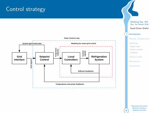
Control strategy

Decentralized Production Units

Distributers(Other Interfaces)

Grid Controller(s)

Aggregators(Service Providers)

Intelligent Consumers

MajorUnits Controvertible

Units

RefrigerationSystem

Local Controllers

SetpointControl

GridInterface

Different feedbacks

Temperatures and power feedbacks

System (grid node) data

Outer Control Loop

Gri

d S

ign

al

Te

mp

retu

re

setp

on

ts

Co

ntr

ol

sig

nal

s

Modeling for smart grid control

30


Seyed Ehsan Shafiei

4 Introduction



Suction manifold

Condenser

System model

Simulations

Simulations


Acknowledgement

I ESO2 project

“ESO2 Optimization of Supermarket Refrigeration Systems”

Lars Norbert Petersen, Henrik Madsenand Christian Heerup

I Danfoss

30


Seyed Ehsan Shafiei

Introduction

5 Booster Configuration


Suction manifold

Condenser

System model

Simulations

Simulations


A typical CO2 booster configuration

Mathematically, the optimal high side pressure PH can be obtainedby solving the following differential equation:

@COP@PH

¼ 0 ð2Þ

To solve Eq. (2), Eq. (1) is rearranged as:

COP ¼ yðh9 � h8Þ þ ð1� yÞðh11 � h10Þh1�h151�x

� �þ ð1� yÞðh12 � h11Þ

ð3Þ

Let,

F1 ¼ yðh9 � h8Þ þ ð1� yÞðh11 � h10Þ ð4Þand,

F2 ¼ ð1� yÞðh12 � h11Þ ð5Þthen,

COP ¼ F1

h1�h151�x

� �þ F2

ð6Þ

Therefore, Eq. (2) is derived as:

@COP@PH

¼@F1@PH

h1�h151�x

� �þ F2

h i� F1

@ h1�h15@PHð Þ@PH

þ @F2@PH

h ih1�h151�x

� �þ F2

h i2 ¼ 0 ð7Þ

Since both F1 and F2 are independent of PH, both@F1@PH

and @F2@PH

equalto zero. Therefore, Eq. (7) can be simplified as:

@ h1�h151�x

� �@PH

¼@ h1s�h15

ð1�xÞgis

h i@PH

¼ 0 ð8Þ

where the isentropic efficiency gis of the high stage compressor canbe calculated as:

gis ¼h1s � h15

h1 � h15¼ A� B� Rp ¼ A 1� B

A� Rp

� �

¼ Að1� Rab � RpÞ ð9Þwhere Rab ¼ B

A.Accordingly, Eq. (8) can therefore be rearranged as:

@ h1s�h15ð1�xÞ�ð1�RabRpÞ

h i@PH

¼ 0 ð10Þ

1.0

10.0

0 100 200 300 400 500 600 700

Pres

sure

(MPa

)

Enthalpy (kJ/kg)

123

47

8

5

10

12

11

614

139 15

1s

Fig. 2. P–H diagram of transcritical cycle in the CO2 booster system.

Gas cooler /Condenser

MT Evaporator

LT Evaporator

TEV_LT

TEV_MT

CV_HP

BPV_2

BPV_1

SHX

REC

COMP_LO

COMP_HI_

12

3

4

7 8

5 6

10

9

11

12

13

14

15

Fig. 1. A typical CO2 booster system applied in supermarket refrigeration system.

1870 Y.T. Ge, S.A. Tassou / Energy Conversion and Management 52 (2011) 1868–1875

[Y.T. Ge, S.A. Tassou, 2011, “Thermodynamic analysis of transcriticalCO2 booster refrigeration systems”]

30


Seyed Ehsan Shafiei

Introduction

6 Booster Configuration


Suction manifold

Condenser

System model

Simulations

Simulations


P–H diagram of transcritical cycle

Mathematically, the optimal high side pressure PH can be obtainedby solving the following differential equation:

@COP@PH

¼ 0 ð2Þ

To solve Eq. (2), Eq. (1) is rearranged as:

COP ¼ yðh9 � h8Þ þ ð1� yÞðh11 � h10Þh1�h151�x

� �þ ð1� yÞðh12 � h11Þ

ð3Þ

Let,

F1 ¼ yðh9 � h8Þ þ ð1� yÞðh11 � h10Þ ð4Þand,

F2 ¼ ð1� yÞðh12 � h11Þ ð5Þthen,

COP ¼ F1

h1�h151�x

� �þ F2

ð6Þ

Therefore, Eq. (2) is derived as:

@COP@PH

¼@F1@PH

h1�h151�x

� �þ F2

h i� F1

@ h1�h15@PHð Þ@PH

þ @F2@PH

h ih1�h151�x

� �þ F2

h i2 ¼ 0 ð7Þ

Since both F1 and F2 are independent of PH, both@F1@PH

and @F2@PH

equalto zero. Therefore, Eq. (7) can be simplified as:

@ h1�h151�x

� �@PH

¼@ h1s�h15

ð1�xÞgis

h i@PH

¼ 0 ð8Þ

where the isentropic efficiency gis of the high stage compressor canbe calculated as:

gis ¼h1s � h15

h1 � h15¼ A� B� Rp ¼ A 1� B

A� Rp

� �

¼ Að1� Rab � RpÞ ð9Þwhere Rab ¼ B

A.Accordingly, Eq. (8) can therefore be rearranged as:

@ h1s�h15ð1�xÞ�ð1�RabRpÞ

h i@PH

¼ 0 ð10Þ

1.0

10.0

0 100 200 300 400 500 600 700

Pres

sure

(MPa

)

Enthalpy (kJ/kg)

123

47

8

5

10

12

11

614

139 15

1s

Fig. 2. P–H diagram of transcritical cycle in the CO2 booster system.

Gas cooler /Condenser

MT Evaporator

LT Evaporator

TEV_LT

TEV_MT

CV_HP

BPV_2

BPV_1

SHX

REC

COMP_LO

COMP_HI_

12

3

4

7 8

5 6

10

9

11

12

13

14

15

Fig. 1. A typical CO2 booster system applied in supermarket refrigeration system.

1870 Y.T. Ge, S.A. Tassou / Energy Conversion and Management 52 (2011) 1868–1875

[Y.T. Ge, S.A. Tassou, 2011, “Thermodynamic analysis of transcriticalCO2 booster refrigeration systems”]

30


Seyed Ehsan Shafiei

Introduction


7 ModelingDisplay cases

Suction manifold

Condenser

System model

Simulations

Simulations


Modular approach

� Display casesI Dynamical equationsI Gray-Box modelingI Simulation and validation

� Suction manifoldI Dynamical equationsI parameter estimationsI Simulation and validation

� CondenserI Dynamical equationsI parameter estimationsI Simulation and validation

30


Seyed Ehsan Shafiei

Introduction


Modeling8 Display cases

Suction manifold

Condenser

System model

Simulations

Simulations


Dynamical equations

MfoodsCpfoodsdTfoods

dt = −Qfoodsair

MwallCpwalldTwall

dt = Qairwall − Qe + Qfan

Mair Cpair � MwallCpwall ⇒ Qfoodsair + Qload − Qairwall = 0

Qfoodsair = UAfoodsair (Tfoods − Tair )

Qairwall = UAairwall (Tair − Twall )

Qload = UAload (Tindoor − Tair )

30


Seyed Ehsan Shafiei

Introduction



Suction manifold

Condenser

System model

Simulations

Simulations


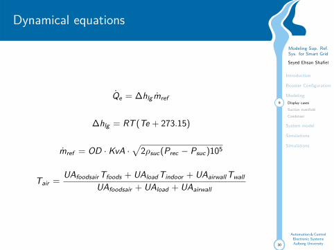
Dynamical equations

Qe = ∆hlgmref

∆hlg = RT (Te + 273.15)

mref = OD · KvA ·√

2ρsuc(Prec − Psuc)105

Tair =UAfoodsair Tfoods + UAloadTindoor + UAairwallTwall

UAfoodsair + UAload + UAairwall

30


Seyed Ehsan Shafiei

Introduction



Suction manifold

Condenser

System model

Simulations

Simulations


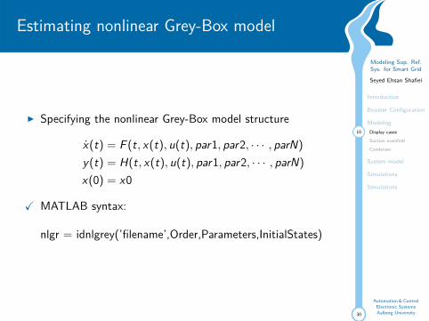
Estimating nonlinear Grey-Box model

I Specifying the nonlinear Grey-Box model structure

x(t) = F (t, x(t), u(t), par1, par2, · · · , parN)

y(t) = H(t, x(t), u(t), par1, par2, · · · , parN)

x(0) = x0

X MATLAB syntax:

nlgr = idnlgrey(’filename’,Order,Parameters,InitialStates)

30


Seyed Ehsan Shafiei

Introduction



Suction manifold

Condenser

System model

Simulations

Simulations


Estimating nonlinear Grey-Box model

I Prediction error minimization method

θ = argminθ

VN(θ)

VN(θ) =N∑

k=1||ydata(k)− y(k)||2

[Lennart Ljung, 2002, “Prediction error estimation methods”]

X MATLAB syntax:

nlgr = pem(data,nlgr)

30


Seyed Ehsan Shafiei

Introduction



Suction manifold

Condenser

System model

Simulations

Simulations


Input-output pair and parameters

I Input-output pair for identification

u =[Psuc Tindoor OD1 · · · ODN

]Ty = [mcr Tair ,1 Twall,1 Tfoods,1 · · · Tair ,N Twall,N Tfoods,N ]T

I predefined parametersPrec = 38, Cpwall = 385, Cpfoods = 1000 (The same as ESO2report)

I To be estimated parametersUAload , UAairwall , UAfoodsair , Mwall , Mfoods , Qfan, KvA

30


Seyed Ehsan Shafiei

Introduction



Suction manifold

Condenser

System model

Simulations

Simulations


Estimation results

UAload =

21.4838.90

3121.4829.1614.638.02

UAairwall =

471.77835.55579.03363.42488.90345.95278.77

UAfoodsair =

84.14141.71146.96174.60351.6958.1895.87

Mwall =

209.06451.38401.14299.31161.19159.27262.23

Mfoods =

2316.46450.4

13364.619112

97939907.45133.4

Qfan =

251.24231.05804.85

5.200.00

436.223.89

KvA = [0.89 1.60 1.50 1.10 2.18 0.57 0.83]× 10−6

30


Seyed Ehsan Shafiei

Introduction



Suction manifold

Condenser

System model

Simulations

Simulations


Estimation results (training data)

02468

Tai

r,1

MeasurementError: 0.71

−20246

Tai

r,2


−202468

Tai

r,3


024

Tai

r,4


−20246

Tai

r,5


02468

Tai

r,6


1 61 121 181 241 301−1

01

Tai

r,7


30


Seyed Ehsan Shafiei

Introduction



Suction manifold

Condenser

System model

Simulations

Simulations


Estimation results (test data)

−20246

Tai

r,1


−20246

Tai

r,2

MeasurementError: 1

−20246

Tai

r,3


024

Tai

r,4


−2024

Tai

r,5

MeasurementError: 1

02468

Tai

r,6

MeasurementError: 1

1 61 121 181 241 301−0.50

0.511.5

Tai

r,7


30


Seyed Ehsan Shafiei

Introduction



16 Suction manifold

Condenser

System model

Simulations

Simulations


Suction manifold dynamical equations

dPsucdt =

mcr + mdist − Vcompρsuc

VsucdρsucdPsuc

Vcomp =cap100 · ηvol · Vd

Wcomp =1

ηcompVcompρsuc(hic − hoe)

hic = hoe +1ηis

(his − hoe)

Vd = 6.5× 70/50 + 120, Vsuc = 2, ηvol =?, ηis =?, ηcomp =?

30


Seyed Ehsan Shafiei

Introduction



17 Suction manifold

Condenser

System model

Simulations

Simulations


Estimating compressor parameters

50 100 150 200 250 300

2

4

6

8

10

12

14

Wcom

p[K

W]

dWcompdWcomp

est

ηvol = 0.535, ηis = 0.836, and ηcomp = 0.465

30


Seyed Ehsan Shafiei

Introduction



18 Suction manifold

Condenser

System model

Simulations

Simulations


Suction manifold simulation

25

26

27

28

Psu

c

Psuc

Psucest

50 100 150 200 250 3002

4

6

8

10

12

Wcom

p[K

W]

dWcomp

dWcompest

u =[Pc mref cap

]T and y =[Psuc Wcomp

]T

30


Seyed Ehsan Shafiei

Introduction



Suction manifold

19 Condenser

System model

Simulations

Simulations


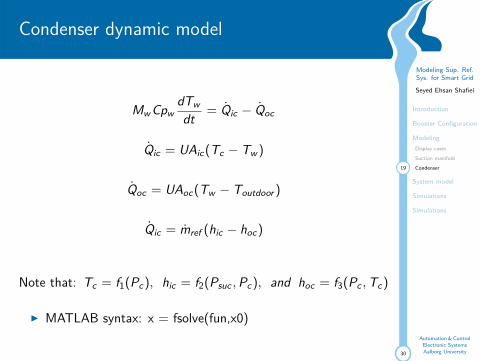
Condenser dynamic model

Mw CpwdTwdt = Qic − Qoc

Qic = UAic(Tc − Tw )

Qoc = UAoc(Tw − Toutdoor )

Qic = mref (hic − hoc)

Note that: Tc = f1(Pc), hic = f2(Psuc ,Pc), and hoc = f3(Pc ,Tc)

I MATLAB syntax: x = fsolve(fun,x0)

30


Seyed Ehsan Shafiei

Introduction



Suction manifold

20 Condenser

System model

Simulations

Simulations


Condenser simulation

50 100 150 200 250 300

44

46

48

50

52

54

56

Pc

Pc

Pcest

u =[mref Toutdoor Psuc

]T and y = Pc

30


Seyed Ehsan Shafiei

Introduction



Suction manifold

Condenser

21 System model

Simulations

Simulations


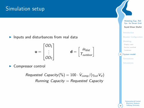
Simulation setup

I Inputs and disturbances from real data

u =

OD1...

OD7

d =

[mdist

Toutdoor

]

I Compressor control

Requested Capacity(%) = 100 · Vcomp/(ηvolVd )

Running Capacity = Requested Capacity

30


Seyed Ehsan Shafiei

Introduction



Suction manifold

Condenser

22 System model

Simulations

Simulations


Modeling results

50 100 150 200 250 300−2

0246

Tcr

1

MeasurementsModel

50 100 150 200 250 300−2

0246

Tcr

2

MeasurementsModel

50 100 150 200 250 300−2

0246

Tcr

3

MeasurementsModel

50 100 150 200 250 300−2

024

Tcr

4

MeasurementsModel

50 100 150 200 250 300−4−2

024

Tcr

5

MeasurementsModel

50 100 150 200 250 30002468

Tcr

6

MeasurementsModel

50 100 150 200 250 300−0.5

00.5

11.5

Tcr

7

MeasurementsModel

30


Seyed Ehsan Shafiei

Introduction



Suction manifold

Condenser

23 System model

Simulations

Simulations


Modeling results

50 100 150 200 250 3000

2

4

6

8

10

Wcom

p[K

W]

MeasurementModel

30


Seyed Ehsan Shafiei

Introduction



Suction manifold

Condenser

System model

24 Simulations

Simulations


Simulation set up

I Time setting

Sampling time = 60 s simulationtime = 2 days

I Solver

ODE45

30


Seyed Ehsan Shafiei

Introduction



Suction manifold

Condenser

System model

25 Simulations

Simulations


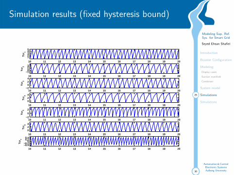
Simulation results (fixed hysteresis bound)

10 11 12 13 14 15 16 17 18 19 20

12345

Tcr

1

10 11 12 13 14 15 16 17 18 19 20

−10123

Tcr

2

10 11 12 13 14 15 16 17 18 19 20−2

024

Tcr

3

10 11 12 13 14 15 16 17 18 19 20

024

Tcr

4

10 11 12 13 14 15 16 17 18 19 20−2

0

2

Tcr

5

10 11 12 13 14 15 16 17 18 19 20

024

Tcr

6

10 11 12 13 14 15 16 17 18 19 20−0.4−0.2

00.20.4

Tcr

7

30


Seyed Ehsan Shafiei

Introduction



Suction manifold

Condenser

System model

26 Simulations

Simulations



10 11 12 13 14 15 16 17 18 19 200

0.5

1

OD

1

10 11 12 13 14 15 16 17 18 19 200

0.5

1

OD

2

10 11 12 13 14 15 16 17 18 19 200

0.5

1

OD

3

10 11 12 13 14 15 16 17 18 19 200

0.5

1

OD

4

10 11 12 13 14 15 16 17 18 19 200

0.5

1

OD

5

10 11 12 13 14 15 16 17 18 19 200

0.5

1

OD

6

10 11 12 13 14 15 16 17 18 19 200

0.5

1

OD

7

30


Seyed Ehsan Shafiei

Introduction



Suction manifold

Condenser

System model

27 Simulations

Simulations



0 5 10 15 20 25 30 35 40 452

4

6

8

10

12

14

16

Wcom

p[K

W]

0 5 10 15 20 25 30 35 40 454

6

8

10

12

14

16

To

utd

oo

r

30


Seyed Ehsan Shafiei

Introduction



Suction manifold

Condenser

System model

28 Simulations

Simulations


Simulation results (varying hysteresis bound)

0 5 10 15 205

1015

To

utd

oo

r

0 5 10 15 20

12345

Tcr

1

0 5 10 15 20

024

Tcr

2

0 5 10 15 20−2

02

Tcr

3

0 5 10 15 20024

Tcr

4

0 5 10 15 20−2

02

Tcr

5

0 5 10 15 20024

Tcr

6

0 5 10 15 20−0.4−0.20

0.20.4

Tcr

7

30


Seyed Ehsan Shafiei

Introduction



Suction manifold

Condenser

System model

29 Simulations

Simulations


Simulation results (varying hysteresis bound)

0 5 10 15 20

4

6

8

10

12

14

16

Wcom

p[K

W]

0 5 10 15 204

6

8

10

12

14

16

To

utd

oo

r

30


Seyed Ehsan Shafiei

Introduction



Suction manifold

Condenser

System model

Simulations

30 Simulations


Future works

� Improving the modelI Modifying the subsystems and parametersI Modeling freezer roomsI Considering opening and closing hoursI Identifying a model for closing hours

� Using the model toI Estimate available thermal capacityI Develop energy storage model/functionI Define system flexibilityI Investigate different control scenariosI · · ·

modeling supermarket refrigeration systems for smart grid...

Documents