Abstract

ICR1SAT (International Crops Research Institute for theSemi-Arid Tropics). 1989. Modeling the Growth and Devel-opment of Sorghum and Pearl Millet. Research Bulletin no. 12.(Virmani, S.M., Tandon, H.L.S., and Alagarswamy, G. eds.).Patancheru, A.P. 502 324, India: ICRISAT.

The 1980s have witnessed substantial increases in food produc-t ion. This has raised expectations that improved systems offarming wil l be rapidly adopted by small farmers in developingcountries. The agroecological environment of such farms isfragile and the fanners are resource-poor. Therefore, strategiesrecommended for increasing food production must be ecologi-cally sound and should result in sustainable agriculture.

System modeling can greatly expedite the search for improv-ed development strategies. Recent advances in crop modelinghave made it possible to simulate yields and growth of severalcrops under varied soil and weather conditions with differentmanagement practices. This bulletin describes the frameworkof CERES (Crop Estimation Through Resource and Environ-ment Synthesis) models developed by the International Bench-mark Sites Network for Agrotechnology Transfer ( IBSNAT)and The International Crops Research Institute for the Semi-Ar id Tropics ( ICRISAT) . Recent work on the simulation ofnitrogen transformation in soils at the International FertilizerDevelopment Center ( IFDC) is discussed. A section on riskanalyzes the cost-benefit implications of various inputs forincreased crop production. RESCAP—a resource capturemodel developed at I C R I S A T Center is presented.

This publication is a cogent source book on the current statusof development of CERES and RESCAP models, their dataneeds, outputs, and applications.

ISBN-92-9066-174-7

The International Crops Research Institute for the Semi-Arid Tropics is a nonprofit , scientific, research and training institutereceiving support f rom donors through the Consultative Group on International Agricultural Research. Donors to I C R I S A T includegovernments and agencies of Austral ia, Belgium, Canada, Federal Republic of Germany, Finland, France, India, Italy, Japan,Netherlands, Norway, Sweden, Switzerland, United Kingdom, United States of America, and the fol lowing international and privateorganizations: Asian Development Bank, Deutsche Gesellschaft fur Technische Zusammenarbeit (GTZ), International DevelopmentResearch Centre, International Fund for Agricul tural Development, The European Economic Community, The Opec Fund forInternational Development, The Wor ld Bank, and United Nations Development Programme. Information and conclusions in thispublication do not necessarily reflect the position of the aforementioned governments, agencies, and international and privateorganizations.

The opinions in this publication are those of the authors and not necessarily those of ICRISAT. The designations employed and thepresentation of the material in this publication do not imply the expression of any opinion whatsoever on the part of I C R I S A Tconcerning the legal status of any country, terr i tory, city, or area, or of its authorities, or concerning the delimitation of its frontiers orboundaries. Where trade names are used this does not constitute endorsement of or discrimination against any product by theInstitute.

Modeling the Growth and Developmentof Sorghum and Pearl Millet

Edited by

S.M. Virmani, H.L.S. Tandon, and G. Alagarswamy

Sponsored by

International Benchmark Sites Network for Agrotechnology Transfer(IBSNAT)

IBSNAT

ICRISAT

International Crops Research Institute for the Semi-Arid Tropics(ICRISAT)

International Fertilizer Development Center(IFDC)

ICRISAT

Research Bulletin no. 12International Crops Research Institute for the Semi-Arid Tropics

Patancheru, Andhra Pradesh 502 324, India

1989

Scientific EditorsS.M. Virmani, H.L.S. Tandon, and G. Alagarswamy

Publication EditorSeth R. Beckerman

Editorial CoordinationSarwat Hussain

Cover DesignSheila Bhatnagar

Data Base ManagementSystems ( D B M S )

Nitrogen in Soils

Soil Water Balanceand Weather Generation

Valuation of Risksto Crop Production

Physiology of Sorghumand Pearl Mil let

Modeling Sorghumand Pearl Mil let

Conclusion

Glossaries

Contents

Foreword

Preface

IBSNAT's Decision Support System for Agrotechnology Trans ferUpendra Singh

Use and Applications of Data Base Management SystemsUpendra Singh and G. Alagarswamy

Discussion

Simulation of Nitrogen Transformation in SoilD C . Godwin

Modeling Nitrogen Uptake and Response in Sorghum and Pear l MilletG. Alagarswamy, Upendra Singh, and D.C. Godwin

Discussion

Description of Soil Water BalanceJ.T. Ritchie and D.C. Godwin

Obtaining Soil Input for the CERES ModelJ.T. Ritchie and D.C. Godwin

Weather Generator ProgramD.C. Godwin

Discussion

Risk AnalysisD.C. Godwin and Upendra Singh

Discussion

Simulation of Sorghum and Pearl Millet PhenologyJ.T. Ritchie and G. Alagarswamy

Genetic Coefficients for the CERES Models J.T. Ritchie and G. Alagarswamy

Discussion

RESCAP: A Resource Capture Model for Sorghum and Pearl M illetJ.L. Monteith, A.K.S. Huda, and D. Midya

Simulation of Growth and Development in CERES ModelsJ.T. Ritchie and G. Alagarswamy

Discussion

Models, Software, and DocumentationJ.T. Ritchie, J.L. Monteith, D.C. Godwin, and A.K.S. Huda

Participants

CERES Glossary, RESCAP Glossary

1

2

3

5

7

8

11

13

14

16

18

20

21

23

24

27

29

30

34

39

40

41

44

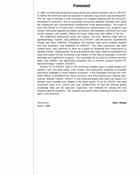
Foreword

In 1982, an international group of agricultural and system scientists met at ICRISATto define the minimum data set required to simulate crop growth and development.The aim was to develop a solid foundation for research dealing with the soil-plant-atmosphere continuum, and to encourage strong links between scientists who studythe biophysical and socioeconomic components of the agroecosystem. The scope ofwork was limited to 10 food crops, including four cereals (maize, rice, sorghum, andwheat), three grain legumes (dry beans, groundnut, and soybean), and three root crops(aroid, cassava, and potato). Barley and pearl millet were later added to the list.

The conference participants wrote two reports. The first, Minimum Data Sets for Agrotechnology Transfer, was published by ICRISAT, and the second, Experimental Design and Data Collection Procedures: the minimum data set for systems analysis and crop simulation, was published by IBSNAT. The latter publication has beenrevised twice, and continues to serve as a guide for designing field experiments tovalidate models. Subsequently, the group decided there was a need to standardize theinput and output format of existing crop models so that they all accessed a commondata base and application program. This eventually led to a plan to combine the database, crop models, and application programs into a Decision Support System forAgrotechnology Transfer (DSSAT).

Version 2.0 of DSSAT used in this workshop enables users to easily access soil,weather, and crop data bases, crop models, and application programs to evaluatealternative strategies to attain desired outcomes. It was developed through the com-bined efforts of scientists from many countries, and international and regional agri-cultural research centers. DSSAT is still being developed and users can expect it tobecome more versatile and reliable in the years ahead. To do so, DSSAT will needcontinued input from current and new collaborators so that the existing globalknowledge base can be captured, organized, and retrieved for solving site and'situation-specific problems. The sorghum and pearl millet modeling workshop is onestep in this direction.

Honolulu, Goro UeharaMarch 1989

Preface

In recent years, crop models have advanced from restricted academic exercises to toolswith potential for wide applications in agriculture. Builders of the CERES series ofmodels, for example, aim at predicting the yield of any genotype, in any soil, at anylocation, and in any weather.

One of ICRISAT's mandates is to identify constraints to agricultural developmentin the semi-arid tropics and evaluate means of alleviating them. Another is to assist inthe development and transfer of technology by sponsoring workshops, conferences,and training programs. It was thus appropriate that ICRISAT, in cooperation withIBSNAT and IFDC, hosted the training workshop on sorghum and pearl milletmodeling.

The aim was to familiarize and train agricultural researchers in the principles andoperational aspects of crop modeling, and obtain feedback about the potential andlimitations of current models.

In an evaluation of the workshop conducted by ICRISAT's Training Program, a majority of the participants gave high marks to the workshop. About two-thirds of therespondents said the number of handouts should be increased, and almost all felt thatthey had benefited from the computer exercises. Exposure to modeling, hands-oncomputer time working with models, and understanding subroutines were identifiedas the areas of greatest benefit.

Participants anticipated continued contact with workshop organizers throughupdates and documentation. They felt there should have been more computer time,more printers and visual aids, more time to discuss group findings from hands-onexercises, and provision of computer manuals and documentation before theworkshop.

Summaries of the papers, discussions, and a list of documents distributed during theworkshop are provided in this report. The Resource Management Program of ICRI -SAT, along with IBSNAT and IFDC, welcomes comments or requests for detailedinformation.

The work of the organizing committees of the three collaborating institutions wasmarked by a constructive spirit. Considerable assistance was received from G. Uehara,T. Tsuji, and J.T. Ritchie representing IBSNAT; D.C. Godwin, L.L. Hammond, andP.L.G. Vlek of IFDC in program planning and the identification of potential partici-pants; and B.C.G. Gunasekera, S.M. Virmani, J.R. Burford, J.W. Estes, J.M. Pea-cock, D.L. Oswalt. G. Alagarswamy, T.J. Rego, and A.K.S. Huda from ICRISAT inhelping to define the objectives and making the preparations for the workshop. Theiradvice and guidance is appreciated. Finally, thanks are due to S.M. Virmani forconceptualizing and coordinating the workshop so efficiently.

ICRISAT J.L. MonteithMarch 1989

2

Data Base Management Systems(DBMS)

IBSNAT's Decision Support System forAgrotechnology Transfer

Upendra Singh

A decision-making system consists of a user who utilizes a system to carry out a task ina given environment. The components of a decision support system are:• a data base;• a model base; and• a control program.

The dialogue generator links the user to each of the above. The system is designed todefine, organize, process, and retrieve information in a way that is useful to the user.The decision support system is intended to provide information effectively andefficiently. Much of the power and flexibility of the system is derived from theinteraction between the system and the user.

The Decision Support System for Agrotechnology Transfer (DSSAT) developed byIBSNAT is a computerized system to help resource planners and farmers makedecisions as they seek solutions to specific agricultural problems. These includeresource allocation, land use planning, and environmental protection. It can predict,diagnose problems, and prescribe appropriate solutions. As an educational tool, ithelps users understand agricultural systems and provides an opportunity to exploreimportant biological, physical, and chemical relationships in agriculture.

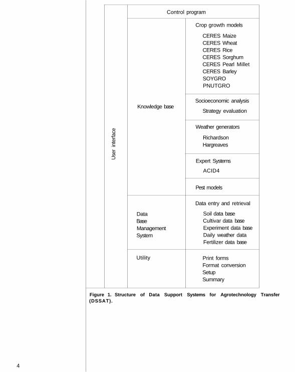
DSSAT provides convenient access to soil, crop, and climatic data bases; cropsimulation models; weather generators; expert systems; strategy evaluation; andutility programs for formatting, retrieving, and graphing information. Crop models,weather generators, expert systems, and strategy analyses form the knowledge base ofDSSAT. DSSAT's modular structure (Fig. 1) and standardized input-output formatlend themselves to incorporation of new models and expert systems to accommodatean expanding knowledge base.

The most important component of DSSAT is the data base, which stores theminimum data set (MDS) for soil, crop, management, and weather data from colla-borators around the world. The convenient, interactive, and efficient access to thesedata facilitates the development, modification, and validation of crop models, expertsystems, and weather generators.

Validation is the cornerstone of evaluation. It ensures that models perform correctlywhen tested against observed data. Validated models can be used to reliably simulatecrop yields and other output variables in different environments. Simulated resultsfrom many years of real-time or generated weather can be used to estimate yieldvariability and risk under alternative management options.

It is envisioned that new models which describe the effects of nutrients other thannitrogen, pests and pesticides, groundwater quality, farming systems, and socioeco-nomic variables will appear within the foreseeable future, and can be accommodatedas DSSAT is further developed. In addition, statistical analysis and other evaluationprograms for model validation, weather generators, and expert systems can be easilycoupled to DSSAT.

With the inclusion of nutrient, pest, and farming systems models, DSSAT will beable to facilitate the design of agrotechnology packages better suited to resources andfarmer objectives. The ultimate objective of DSSAT is to improve the decision-making ability of farmers.

3

4

Use

r in

terfa

ce

Control program

Knowledge base

DataBaseManagementSystem

Utility

Crop growth models

CERES MaizeCERES WheatCERES RiceCERES SorghumCERES Pearl MilletCERES BarleySOYGROPNUTGRO

Socioeconomic analysis

Strategy evaluation

Weather generators

RichardsonHargreaves

Expert Systems

ACID4

Pest models

Data entry and retrieval

Soil data baseCultivar data baseExperiment data baseDaily weather dataFertilizer data base

Print formsFormat conversionSetupSummary

Figure 1. Structure of Data Support Systems for Agrotechnol ogy Transfer(DSSAT).

Reference

Use and Applications of Data Base ManagementSystems

Upendra Singh and G. Alagarswamy

A data base management system (DBMS) is designed to organize and store data,provide user-friendly data entry and retrieval programs, and integrate data fromseveral sources into a computerized system. It also provides an interface between thedata base and specific application programs with a control program, usually referredto as a data base processing system. A well-designed DBMS occupies as little diskspace as possible, can be quickly searched, indexed or queried, and answers users'questions easily, including those that its designers had not anticipated. It also helpsusers avoid data errors, and provides a means to check and account for data integrity.In order to be effective, a DBMS requires a symbiosis between the users and thesystem.

The DBMS component of DSSAT is a relational data base. Thus, the informationneeded to support agrotechnology transfer functions is stored in a group of relateddata base files. These files store data on site weather, experimental details, soil pedon,profile description, and crop-specific genetic coefficients. The coded forms (A-S) inIBSNAT Technical Report 1 (1988) describe these and data collection methods. Thefiles are related by common key index fields in such a way that data can be retrieved asrequired. The key indices used are crop identification (ID), institute ID , site I D , andexperiment ID. Together the related data base files function as a larger data base, andreduce redundancy (Fig. 1).

The advantages of relational DBMSs become evident when considering weatherdata files. The weather data are filed separately from experimental data because thesame weather station data can be used for more than one experiment at the same site.Separate storage conserves computer memory and disk space. Several years ofweather data collected at one site is easily accessible, allowing models to be testedunder varying climatic conditions. This also allows creation of weather coefficients forweather generators, and to perform long-term simulation experiments. Every experi-mental data set can be rejoined to its weather station data set when required for cropsimulation, since it is cross-indexed by site and weather ID codes, and duration ofexperiment. A similar functional relationship exists between experimental and soildata.

One major application of the minimum data set (MDS) stored in the DBMS istesting the performance of crop models. Model- specific input data files and validationfiles are created by retrieving the MDS from the data base (Fig. 1). Other applicationsare: statistical analysis, plotting results, input to expert systems, input to site-specificmodels, etc. The DBMS program also provides output on weather, experiment, andsoil inputs; graphic display of weather inputs; utility programs for updating oldversions of DBMS and MDS forms; and converting weather and harvest data fromASCII to MDS format. As illustrated in Figure 1, all the files (directory, input, andvalidation data) needed for simulating crop growth are simulated by the DBMS.

IBSNAT (International Benchmark Sites Network for Agrot echnology Transfer).1988. Experimental design and data collection procedures for IBSNAT: the minimumdata set for systems analysis and crop simulation. 3rd edn. Technical Report 1.Honolulu, H I , USA: IBSNAT. 74 pp.

5

6

Minimum Data Set Retrieval Crop Model Files File description DirectoryEntry program Input - Validation (e.g., sorghum)

Manual

Utilityprogram

Site

Weatherdata

Form C

Weatherdataretrieval

File I Daily weather(CSKA06I8.W7I)

Weather•directory(WTH.DIR)

File 4 Crop residue(CSKA7101.SG4)

File 5

File 6

File 7

File 8 Experimentdata

Forms A-S

Experimentdataretrieval

File A

File B

File C

File D

File 2 Soildataretrieval

Soilprofiledescription

Manual

SCSdata base

Soil initial N and water(CSKA7I0I.SG5)

Irrigation(CSKA710I.SG6)

N fertilizer(CSKA7IOI.SG7)

Management(CSKA710I.SG8)

Yield components

Seasonal observation for:

Growth (CSKA7I01.SGB)

Water (CSKA7I0I.SGC)

Nitrogen (CSKA7101.SGD)

Soil profile(SPROFILE.SG2)

Variety(GENET1CS.SG9)

File .1 is not presently used

Figure 1. Schematic representation of a data base manage ment system (DBMS).

File 9 Geneticcoefficients

Experiment-directory(SGEXP.D1R)

Discussion

In the discussion following the presentations, the importance of model validation wasstressed. Model validation evaluates whether or not a model predicts correct results.Questions from the participants centered around terminology, and stressed the need toclarify the terms validation, verification, calibration, and corroboration.

Validation was explained as the process of building the right system, i.e., the systemoutput clearly represents the real situation being modeled.

Verification refers to the mechanics of model building, and the correctness of thecomputations within the model.

Calibration is the process of modifying certain model parameters to more closelyreflect local weather and soil conditions, etc.

Finally, corroboration refers to the testing of the predictive capability of a model byan independent third party.

It was agreed that IBSNAT would be requested to publish standard definitions ofthese terms to be used in all future modeling projects and workshops.

It was stressed that having a model does not mean that experimentation stops.Rather, experiments must still be performed, and real measurements must be com-pared with simulated measurements, so that models can be perfected. Simulatedmeasurements cannot always be the same as real measurements, since a change in a single factor can produce different results. This was demonstrated by photographs ofthe same crop sown on the same day at locations at three different elevations.

The main areas of application of DSSAT were:• research, where it forms a framework for setting priorities and guiding research,

and helps evaluate the potential of agrotechnology;• training, where it can present and reinforce concepts and principles of agrotechnol-

ogy, demonstrate the application of biological processes, and provide the basis forcomputer-designed laboratory exercises; and

• extension, where it provides a basic structure for extension of knowledge.The need for a minimum data set, the basic data required for models to work

properly, was stressed. Different computer-based forms for entering data into DSSATwere demonstrated.

7

Movement of Nitrateand Urea

Fertilizer Additionsand Urea Hydrolysis

Mineralization andImmobilization

8

Nitrogen in SoilsSimulation of Nitrogen Transformation in Soil

D.C. Godwin

The nitrogen (N) component of the model is designed to operate as a component of theCERES models and not in a stand-alone mode. The soil N submodel describes theprocesses of mineralization and/or immobilization of N associated with the decay ofcrop residues, nitrification, denitrification, urea hydrolysis, leaching of nitrate, andthe uptake and utilization of N by the crop. It utilizes the layered soil water balancemodel described in this publication and a simple soil temperature subroutine. The soilN model comprises two subroutines describing N movement, and soil N transforma-tions. Additional subroutines are used for input and output of data and for theinitialization of the various N pools.

Ammonium is assumed not to be transported across soil layers. Only the movement ofnitrate and urea is considered. The same procedures for simulating nitrate movementare used for urea movement. Nitrate movement in the soil profile is dependent uponwater movement. In the water balance component of the model, the volume of watermoving from a layer (L) to the layer below [FLUX(L) ] is calculated. The volume ofwater present in the layer before drainage occurred is also calculated from thevolumetric water content [SW(L)] and the depth of the layer [DLAYR(L) ] . Nitratelost from each layer (NOUT) is then calculated as a function of the water which isretained and that which is moved.

NOUT = SN03(L) * FLUX(L) / (SW(L) * DLAYR(L) + FLUX(L)) (1)

SN03(L) = quantity of nitrate present in layer L (kg N ha-1)-

A simple cascading approach is used where the nitrate lost from one layer is addedto the layer below. When the concentration of nitrate in a layer falls to 1.0 g N0 3 g

-1

of soil, no further leaching from that layer is allowed to occur. Most of the differencesin simulated nitrate leaching rate between soils of different texture is explained by thedifference in proportion of water which is mobile.

Similar procedures are used to simulate the rate of upward movement of nitrate andurea with evaporation of water from the surface layers. In this case the water balanceroutine calculates the upward flow of water [FLOW(L)] and the amount of upwardmovement (NUP) is calculated as for NOUT.

NUP = SN03(L) * FLOW(L) / (SW(L) * DLAYR(L) + FLOW(L)) (2)

Fertilizer N is partitioned in the model between amide, nitrate, and ammonium pools,according to the nature of the fertilizer used. The assumption is that N is uniformlyincorporated into the soil layer into which it is placed. Surface N applications aretreated as being uniformly incorporated into the top layer. Up to 10 split applicationscan be accommodated by the model.

To simulate urea hydrolysis, a maximum hydrolysis rate is estimated from the soilorganic carbon and pH. The temperature and soil water indices are designed tosimulate the effects of soil moisture and temperature.

A balance exists between the two processes of mineralization and immobilization.When crop residues with a high C:N ratio are added to soil, the balance can shifttowards net immobilization for a period of time. After some of the soil carbon has

been consumed by respiration, net mineralization may resume. Nitrogen mineralizedfrom the soil organic pool often constitutes a large part of the N available to the crop.

In the case of residues having a high C:N ratio (e.g., freshly incorporated wheatstraw), the N available for the decay process will greatly limit the decay rate. For eachof the fresh organic matter (FOM) pools a decay rate appropriate for that pool (JP)can be calculated by multiplying the rate constant by the three indices.

G l = T F * M F * C N R F * RDECR(JP) (3)where

G1 = the proportion of the pool which decays in one day,TF = temperature factor,

MF = moisture factor, andCNRF = carbon to nitrogen ratio factor.

The amount of material decayed is then the product of G1 and the pool size.The gross mineralization of N associated with this decay (GRNOM) is thencalculated according to the proportion of the pool which is decaying.

GRNOM = Gl * FPOOL(L,JP) / FOM(L) * FON(L) (4)whereFPOOL(L,JP) = pool of either carbohydrate (JP = 1), cellulose (JP = 2), or lignin

(JP = 3) present in layer L ( g ha-1); andFON = fresh organic nitrogen.

GRNOM is summed for each of three pools in each layer. Similarly, the amount oforganic matter decaying (GRCOM) is determined as the sum of three pool fractions.

The procedure used for calculating the N released from the humus (RHMIN) alsoutilizes TF and MF. In this case CNRF is not used and the potential decay rateconstant (DMINR) is very small (8.3E - 5.0). D M O D is a zero to unity factor foradjusting the mineralization rate on unusual soils. Except for certain volcanic ash andfreshly cultivated virgin soils, a value of 1.0 is used for D M O D . Satisfactory alterna-tives for estimating D M O D are currently being sought. R H M I N is the product of thevarious indices and the N contained within the humus [NHUM(L) ] .

R H M I N = NHUM(L) * D M I N R * TF * MF * D M O D (5)

These calculations also allow for the transfer of 20% of the gross amount of N released by mineralization of FON(L) to be incorporated into NHUM(L) . Thisaccounts for N incorporated into microbial biomass (Seligman and van Keulen 1981).The N which is immobilized into microbial biomass during decay process (RNAC) iscalculated as the minimum of the soil extractable mineral N (TOTN) and the demandfor N by the decaying FOM(L).

RNAC = A M I N l ( T O T N , GRNOM * [0.02 - FON(L) / FOM (L)] 1 (6)whereAMIN1 is a Fortran library function to select the minimum of those variables inparentheses, and 0.02 is the N requirement for microbial decay of a unit ofFOM(L). The value of 0.02 is the product of the fraction of C in the FOM(L) (40%),the biological efficiency of C turnover by the microbes (40%) and the N:C ratio ofthe microbes (0.125). FOM(L) and FON(L) are then updated:

FOM(L) = FOM(L) - GRCOM (7)

FON (L) = FON(L) + RNAC - G R N O M (8)

In CERES models four pools of organic matter are considered. First, fresh organicmatter (FOM) derived from crop residues is partitioned into three pools—carbo-hydrate, cellulose, and lignin. The fourth organic N pool is derived from stable organicmatter or humus. For each of the FOM pools a decay rate can be calculated bymultiplying a constant rate by three indices. The indices describe the limitations on

9

Nitrification

References

10

decay rate imposed by moisture, temperature, and C:N ratio of the material. Thebalance between RNAC and GRNOM determines whether net mineralization orimmobilization occurs. The net N released from all organic sources (NNOM) is:

NNOM = 0.8 * GRNOM + R H M I N - RNAC (9)

Only 80% of GRNOM enters this pool since 20% was incorporated into NHUM(L) .NNOM can then be used to update the ammonium pool [SNH4(L)].

SNH4(L) = SNH4(L) + NNOM (10)

If net immobilization (NNOM negative) occurs, ammonium is first immobilized. Ifthere is not sufficient ammonium to retain this pool with a concentration of 1 g, thenwithdrawals are made from the nitrate pool.

The potential nitrification rate is a Michaelis-Menten kinetic function dependent onlyon ammonium concentration and is thus independent of soil type. The approach usedin the CERES models has been to calculate a potential nitrification rate and a series ofzero to unity environmental indices to reduce this rate. A further index, termed a "nitrification capacity" is used to introduce a lag effect on nitrification if conditions inthe last 2 days have been unfavorable for nitrification. Actual nitrification capacity iscalculated by reducing the potential rate by the most limiting of the environmentalindices and the capacity index.

The approach adopted in the CERES models has been to adapt the functionsdescribed by Rolston et al. (1980) to fit within the framework of the model and tomatch inputs derived from the water balance and mineralization components ofCERES models.

Denitrification calculations are only performed when the soil water content (SW)exceeds the drained upper limit (DU L). A zero to unity index (FW) for soil water in therange from DUL to saturation (SAT) is calculated.

FW = 1.0 - [SAT(L) - SW(L)] / [SAT(L) - DUL(L)] (11)

A factor for soil temperature is also calculated

FT = 0.1 * EXP[0.046 * ST(L)] (12)

Soil soluble carbon provides the energy for denitrification. This is estimated fromorganic carbon and fresh residues. Denitrification rate (DNR ATE) is calculated fromthe nitrate concentration and converted to a kg N ha"1 day-1 basis for the mass balancecalculations.

DNRATE = 6.0 * 1.0E - 5.0 * CW * N03(L) * FW * FT * DLAYR(L) (13)whereDLAYR(L) = depth of layer L (cm),

FT = temperature factor effect on denitrification (unitless),FW = water factor effect on denitrification (unitless),

N03(L) = nitrate concentration in layer L ( g N g-1 soil), andCW = total water-extractable carbon in the soil layer ( g C g-1 soil).

Rolston, D.E., Sharpley, A.N., Toy, D.W., Hoffman, D.L ., and Broadbent, F.E.1980. Denitrification as affected by irrigation frequency of a field soil. EPA-600/2-80-66. Ada, Oklahoma, USA: U.S. Environmental Protection Agency, pp 58.

Seligman, N.C., and van Keulen, H. 1981. PAPRAN: a simulation model of annualpasture production limited by rainfall and nitrogen. Pages 192-221 in Simulation ofnitrogen behaviour of soil-plant systems (Frissel, M.J., and van Veen, J.A., eds.).Wageningen, Netherlands: PUDOC (Centre for Agricultural Publishing andDocumentation).

Critical N Concentrationin Plant and Deficit Factor

Nitrogen Uptake

Modeling Nitrogen Uptake and Response inSorghum and Pearl Millet

G. Alagarswamy, Upendra Singh, and D.C. Godwin

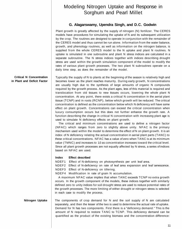
Plant growth is greatly affected by the supply of nitrogen (N) fertilizer. The CERESmodels have procedures for simulating the uptake of N and its subsequent utilizationby the crop. The routines are designed to operate in conjunction with the remainder ofthe CERES model and thus cannot be run alone. Information from the water balance,growth, and phenology routines, as well as information on the nitrogen balance, issupplied from the whole CERES model to the N uptake and plant N routines. N uptake is simulated in one subroutine and plant N stress indices are calculated in a separate subroutine. The N stress indices together with indices describing droughtstress are used within the growth simulation component of the model to modify therates of various plant growth processes. The two plant N subroutines operate on a daily time step, as does the remainder of the model.

Typically the supply of N to plants at the beginning of the season is relatively high andbecomes lower as the plant reaches maturity. During early growth, N concentrationsare usually high due to the synthesis of large amounts of organic N compoundsrequired by the growth process. As the plant ages, less of this material is required andtranslocation from old tissues to new tissues occurs, lowering the whole plant N concentration. At any point, there exists a critical N concentration in the aerial planttissue (TCNP) and in roots (RCNP), below which growth will be reduced. The criticalconcentration is defined as the concentration below which N deficiency will have someeffect on plant growth. Concentrations can exceed the critical concentration whenluxury consumption occurs but this does not further enhance the growth rate. A function describing the change in critical N concentration with increasing plant age isused to simulate N deficiency effects on plant growth.

The critical and minimum concentrations are used to define a nitrogen factor(NFAC) which ranges from zero to slightly above unity. NFAC is the primarymechanism used within the model to determine the effect of N on plant growth. It is anindex of N deficiency relating the actual concentration in aerial plant parts (TANC) tothese critical concentrations. NFAC has a value of zero when TANC is at its minimumvalue (TMNC) and increases to 1.0 as concentration increases toward the critical level.Since all plant growth processes are not equally affected by N stress, a series of indicesbased on NFAC are used.

Index Effect describedNDEF1 Effect of N-deficiency on photosynthesis per unit leaf area.NDEF2 Effect of N-deficiency on rate of leaf area expansion and leaf senescence.NDEF3 Effect of N-deficiency on tillering.NDEF4 Modification in rate of grain N accumulation.

A maximum NFAC value implies that when TANC exceeds TCNP no extra growthoccurs. In the growth component of the models, these indices together with similarlydefined zero to unity indices for soil drought stress are used to reduce potential rates ofthe growth processes. The more limiting of either drought or nitrogen stress is selectedin each case to modify the process.

The components of crop demand for N and the soil supply of N are calculatedseparately, and then the lesser of the two is used to determine the actual rate of uptake.Demand for N has two components. First there is a "deficiency demand." This is theamount of N required to restore TANC to TCNP. This deficiency demand can bequantified as the product of the existing biomass and the concentration difference:

11

12

T N D E M = TOPWT * (TCNP - TANC) (1)whereT N D E M = plant tops N demand (kg N ha-1)TOPWT = weight of aerial plant parts (kg ha-1).

Similarly, for roots the discrepancy in concentration (difference between RCNPand RANC) is multiplied by the root biomass (RTWT) to calculate the root N demand (RNDEM).

RNDEM = RTWT * (RCNP - RANC) (2)

If luxury consumption of N has occurred such that TANC is greater than TCNPthen these demand components have negative values. If total N demand is negativethen no uptake is performed on that day. As biomass increases with crop growth, plantN concentration falls. Thus, when TANC is greater than TCNP, a period of growthwill generally cause TANC to fall toward or below TCNP.

The second component of N demand is the demand for N by the new growth. It isassumed that the plant would attempt to maintain a critical N concentration in thenewly formed tissues. To calculate the new growth demand, a potential amount of newgrowth is first estimated in the GROSUB subroutine. New growth is estimated frompotential photosynthesis. This potential growth increment provides a mechanism forTANC to exceed TCNP. This occurs when some stress prevails, and the actual growthincrement is less than the potential.

During the early stages of plant growth the new growth component of N demandwill be a large proportion of the total demand. As the crop biomass increases, thedeficiency demand becomes the larger component. During grain filling, the N requiredby the grain is removed from the vegetative and root pools to form a grain N pool. Theresultant, lowered concentration in these pools may lead to increased demand. Thetotal plant N demand is the sum of all of these demand components.

To calculate the potential supply of N to the crop, zero to unity availability factorsfor both nitrate and ammonium are calculated from the soil concentrations of theirrespective ions. A zero to unity soil water factor which reduces potential uptake iscalculated as a function of the relative availability of soil water.

The maximum potential N uptake from a soil layer may be calculated as a functionof the maximum daily uptake per unit length of root, and the total amount of rootspresent in the layer. The calculation used integrates the effects of root length density,the soil water factor described above, and the depth of the layer. The effect of ionconcentration and the maximum uptake per unit length of root are also incorporatedinto the calculation.

Potential N uptake from the whole profile (TRNU) is the sum of potential nitrateand potential ammonium uptake from each soil layer where roots occur. Thus TRNUrepresents an integrated value which is sensitive to rooting density, the concentrationof the two ionic species, and their ease of extraction as a function of the soil waterstatus of the different layers. This method of determining potential uptake enables thecondition of nutritional drought to be simulated. Nutritional drought occurs whennutrients and roots are concentrated in the upper layers of the soil profile, butsufficient water for growth and uptake is present only in the lower layers.

If TRNU is greater than the crop N demand (ANDEM), an N uptake factor (NUF)is calculated and used to reduce the N uptake from each layer to the level of demand.

NUF = A N D E M / TRNU (3)

This could occur when plants are young and have a high N supply. If the demand isgreater than the supply, then NUF has a value of 1.0, When NUF is less than 1.0,uptake from each layer is reduced. Following uptake, concentrations of N in both theshoots and roots are updated. Partitioning of the N taken up between shoot and rootparts occurs on the basis of the proportions of the total plant demand arising fromshoots and roots, respectively.

D i s c u s s i o n

The presentations generated a discussion that reflected the importance on N in cropproduction. A doubt was raised about assuming that all the reactions in the N cycle(mineralization, immobilization, etc.) are continuously occurring in the soil. It wasexplained that all the measurements for simulating N behavior are on a daily rate basisin which the previous day's history is considered to simulate events of the followingday.

Regarding the effect of root exudates on N mineralization and its availability toplants, it was pointed out that its occurrence and magnitude is poorly understood. A suggestion was made for verifying the N mineralization rate by actual crop uptake of N from unfertilized plots and measured N mineralization rates, which was agreed.

The use of law of minimum for urea hydrolysis rather than the multiplicativeapproach (used for mineralization) was questioned. It was stated that there was a needto be uniform in computing different aspects of the N cycle. Questions were also raisedabout the decomposition of soil organic matter in the top soil layer when the soil is dryand desiccated. One opinion was that ammonification may continue at a very slow rateunder such conditions, but nitrification may not occur because of high temperature. Itwas also mentioned that the N mineralization rate was slower at soil saturation. It wassuggested that the base for validating nitrogen transformation for concept formationshould be further enlarged. A suggestion was also made to account for the interactionsamong several factors.

Replies to other questions provided these details of the model:When integrating the effects of temperature and moisture on urea hydrolysis, urea

hydrolysis is computed on a daily rate basis because plant growth is modeled on a dailybasis.

In a situation where nitrate could either be leached or denitrified, and whether it iscounted in both processes or not, water in the model moves through the soil layers andleaches nitrates, after which mineralization and other processes are considered, in thatorder. The model at present ignores N losses through ammonia volatilization.

The model assumes that N is available as NH 4 and N0 3 , and does not distinguishbetween the two. In response to the question of why mass flow influence on nitrate hadnot been considered, it was stated that uptake is simulated by root growth and rootloss. Mass flow and diffusion as such are not considered for uptake.

There was a good discussion on the effects of photosynthesis on leaf area expansion.It was stated that the rate of leaf area expansion depends on photosynthesis, and whilethe effect of N on crop phenology was not clear, it may not be large, like that ofphosphorus. It was also suggested that the reduced leaf expansion helps to maintain N requirement.

The model makes no provision to account for the loss of N through plant foliage,but leaf senescence is considered a function of stress. When partitioning N between themain and secondary tillers, the main tiller gets the N first, with remaining N sent to thesecondary tillers.

13

Infiltration and Runoff

Drainage

14

Soi l Water Balance

and Weather Generat ion

Description of Soil Water Balance

J.T. Ritchie and D.C. Godwin

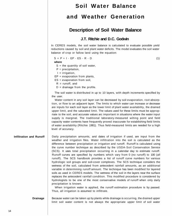
In CERES models, the soil water balance is calculated to evaluate possible yieldreductions caused by soil and plant water deficits. The model evaluates the soil waterbalance of crop or fallow land using the equation:

S = P + I - EP - ES - R - D (1)where

S = the quantity of soil water,P = precipitation,I = irrigation,

EP = evaporation from plants,ES = evaporation from soil,

R = runoff, andD = drainage from the profile.

The soil water is distributed in up to 10 layers, with depth increments specified bythe user.

Water content in any soil layer can be decreased by soil evaporation, root absorp-tion, or flow to an adjacent layer. The limits to which water can increase or decreaseare inputs for each soil layer as the lower limit of plant water availability, the drainedupper limit, and the saturated limit. The values used for these limits must be approp-riate to the soil, and accurate values arc important in situations where the water inputsupply is marginal. The traditional laboratory-measured wilting point and fieldcapacity water contents have frequently proved inaccurate for establishing field limitsof water availability (Ritchie 1981). Thus field-measured limits are needed for a highlevel of accuracy.

Daily precipitation amounts, and dates of irrigation if used, are input from theweather and irrigation files. Water infiltration into the soil is calculated as thedifference between precipitation or irrigation and runoff. Runoff is calculated usingthe curve number technique as described by the USDA-Soil Conservation Service(SCS). It uses total precipitation occurring in a calendar day to estimate runoff.Runoff curves are specified by numbers which vary from 0 (no runoff) to 100 (allrunoff). The SCS handbook provides a list of runoff curve numbers for varioushydrologic soil groups and soil-cover complexes. The SCS technique considers thewetness of the soil, calculated from antecedent rainfall amounts, as an additionalvariable in determining runoff amount. The technique has been modified for layeredsoils as used in CERES models. The wetness of the soil in the layers near the surfacereplaces the antecedent rainfall condition. This modified procedure is considered byhydrologists to be one of the most conservative models of runoff when only dailyprecipitation is known.

When irrigation water is applied, the runoff estimation procedure is by passed.Thus, all irrigation is assumed to infiltrate.

Because water can be taken up by plants while drainage is occurring, the drained upperlimit soil water content is not always the appropriate upper limit of soil water

Evapotranspiration

Root Water Absorption

availability. Many productive agricultural soils drain quite slowly, and may thusprovide an appreciable quantity of water to plants before drainage practically stops. InCERES models, drainage rates are calculated using an empirical relation that evalu-ates field drainage reasonably well.

The drainage formula assumes a fixed saturated volumetric water content (SAT),and fixed drained upper limit water content (DUL). Thus drainage takes place whenthe water content (SW) is between those two limits. The equation is:

DRAIN = SWCON * (SW - DUL) * DEPTH, SW > DUL (2)or

DRAIN = 0, SW < D U L (3)whereSWCON = drainage coefficientDEPTH = the thickness of the soil layer being considered, and

SW = the current water content of the layer.

In the model, constant drainage for one day is assumed and the value SWCONrepresents the fraction of water between DUL and SW that drains in one day.

Evapotranspiration (ET) is calculated using procedures described by Ritchie (1972).The procedure separates soil evaporation (ES) from transpiration (EP) for plantsgrowing without a shortage of soil water. Potential ET is calculated using an equilib-rium evaporation concept, for which a relatively simple empirical equation wasdeveloped. The equation calculates the approximate daytime net radiation andequilibrium evaporation, assuming that stomata are closed at night and no ET occurs.Potential ET is calculated as the equilibrium evaporation multiplied by 1.1 to accountfor the effects of unsaturated air. The multiplier is increased above 1.1 to allow foradvection when the maximum temperature is greater than 35° C, and reduced below1.1 for temperatures below 7°C to account for the influe nce of cold temperatures onstomatal closure.

The calculation of ES when the soil is drying in the original model (Ritchie 1972)was altered for CERES models to further reduce ES when the soil water content in theupper layer reaches a fixed, low-threshold value. This modification was needed toprevent the surface soil from drying too much when roots are also removing water nearthe surface.

The CERES model calculates root water absorption using an approach in which thelarger of the soil or the root resistance determines the maximum possible flow rate ofwater into roots. The soil-limited water absorption rate considers radial flow to singleroots as a function of soil hydraulic conductivity, an assumed daily averaged constantwater potential between root surface and the bulk soil, an assumed constant rootradius, and the root length density. The hydraulic conductivity is normalized for allsoils by assuming a constant value of 5 * 10-6 cm d-1 at the lower limit water content.For water content values above the lower limit, the conductivity increases exponen-tially in proportion to the product of a soil texture dependent coefficient and the watercontent above the lower limit value. The maximum daily absorption rate is assumed tobe 0.03 cm3 cm-1 of root. The soil- or plant-limited maximum absorption rate is thenconverted to an uptake rate for an individual soil layer using the root length densityand the depth of the soil layer. Root length density and distribution in the soil areestimated in CERES models on the basis of soil properties and the amount ofassimilate partitioned to roots. The sum of the maximum root absorption from eachsoil depth gives the maximum possible uptake from the profile. If the maximumuptake exceeds the maximum calculated transpiration rate, the maximum absorptionrates calculated for each depth are reduced so that the uptake becomes equal to thetranspiration rate. If the maximum uptake is less than the maximum transpiration,transpiration rate is set equal to the maximum absorption rate.

15

References

Single Profile Properties

16

We recognize that a weak part of CERES, and of crop models in general, is theestimation of the dynamics of root growth in the soil. Some assumptions that aredifficult to verify experimentally have to be used to simulate root growth patterns. Thegrowth patterns depend on soil physical and chemical properties, the amount ofassimilate transported to the roots, and soil water content. More quantitative rootgrowth information is needed before major improvement can be made in the rootgrowth part of CERES models. Greater details on the water balance model arereported in Ritchie (1985).

Ritchie, J.T. 1972. Model for predicting evaporation from a row crop with incompletecover. Water Resources Research 8:1204.

Ritchie, J.T. 1981. Soil water availability. Plant and Soil 58:327-338.

Ritchie, J.T. 1985. A user-orientated model of the soil water balance in wheat. Pages293-305 in Wheat growth and modeling (Day, W., and Atkin, R.K., eds.). New York,USA: Plenum.

Obtaining Soil Input for the CERES Model

J.T. Ritchie and D.C. Godwin

The soil inputs needed in CERES models can be categorized into those that influence:• water entry and retention in soil,• water loss by evaporation.• the limits of water retention capacity, and• the environment for root growth.

They can be further categorized into single properties needed for the whole soilprofile, and those that vary with depth.

Infiltration of water into the soil is calculated as the difference between precipitationand runoff. Runoff is calculated using the USDA-Soil Conservation Service (SCS)procedure known as the curve number technique. The procedure uses total precipita-tion in a calendar day to estimate runoff.

To determine the runoff curve number for crop land soils, it is necessary to decidewhich of four hydrologic soil groups best describes the soil. The hydrologic groupsinclude four categories for potential runoff: A = low, B = moderately low, C = moderately high, and D = high. The curve number (CN2) is determined from the slopeof the site and the hydrologic category. The curve number is then modified for thedegree of conservation practices followed.

Other inputs for the CERES models can be obtained with either field-measured orapproximated values. If field testing is conducted, field measurements are essential.

The albedo is the measured fraction of the incoming solar radiation that is reflectedback into the atmosphere. Soil albedo can be measured with a specially shieldedsolarimeter pointed toward the ground. If measurements are not possible, the soilalbedo values can be approximated from the color of the upper horizon. These rangefrom about 0.09 for black soils to about 0.18 for light soils.

The stage 1 evaporation constant (U) can be measured with weighing lysimeters,

The Limits ofSoil Water Availability

when the soil is bare and wet. It can also be approximated by measuring the differencebetween the near-surface soil temperature and air temperature, also when the soil iswet and bare. The difference in soil-air temperature, assuming the soil is not shadedby clouds, will be small during first stage evaporation but will increase rapidly once thefirst stage ends. The cumulative potential evaporation from the time the soil wasthoroughly wetted until the end of first stage is the value U. The value ranges fromabout 5 mm for coarse-textured soils and some self-mulching clay soils to about 15mm for clay loams. If soils are poorly drained, U is increased.

The drainage evaluation requires the input soil water content values of drainedupper limit (DUL) and saturation (SAT). Field saturation can be measured byproviding conditions for water to stand on a plot until the soil water content no longerincreases through all soil depths of the root zone. Under these conditions, the bestresults are obtained from properly calibrated neutron soil water probes. After SAThas been determined, water is no longer added to the soil surface and an imperviouscover is placed over the soil to prevent evaporation. Measurements of the soil watercontent during drainage provide the information needed to calculate a drainagecoefficient (SWCON). When the soil water content practically stops draining, thedrained upper limit (DUL) is reached.

If measurements of SAT and SWCON are not available, they can be approximatedfrom soil classification information. The value for SAT is assumed to be 85% of totalporosity and SWCON can be approximated from the permeability classes availablefrom soil. Values of SWCON can vary from 0.85 for very rapid to 0.01 for very slowpermeability.

The DUL values can be measured from the drainage experiment for evaluating the soildrainage coefficient.

The lower limits of moisture content (LOL) are derived from successive measure-ments of soil water content with depth during a period when a field crop was subjectedto severe drought stress. Water content measurements are continued until the plantnearly dies or becomes dormant. Data from adequately fertilized field plots in whichplants reach maximum vegetative growth before undergoing severe drought stress arepreferred over data from plots inadequately fertilized or subjected to early-seasonstress. The concept is that roots have an opportunity to extend to the maximum depthpossible.

With this method one can determine the maximum depth of soil water extraction,which usually will become the lowest soil depth considered in the soil data base. Thisdefinition of LOL biases the near-surface measurements because soil evaporationreduces soil water content below LOL. Also, in deep soils there is practically always anincomplete root water extraction and the water content usually does not reach theLOL value. The depth at which root water extraction is usually incomplete varies insoils from about 1.2 m to 1.5 m.

To estimate the LOL values for these two situations, approximations from otherdepths where values are known can be used. Otherwise estimates based on soil textureare needed.

Empirical equations have been developed to estimate the limits of water extractionwhere the limits are unknown. The equations are based on a data base of severalhundred field-measured limits as reported by Ratliff et al. (1983). The calculations arebased on sand, silt, and clay content, and are modified when values of soil organicmatter are above 0.2%, when the coarse fragment above 2 mm is significant, and whenthe bulk density varies from a "normal" one expected for the soil texture beingconsidered. The estimates of the LOL and DUL with this texture-based procedure aresubject to some error, but the difference between DUL and LOL, the PLEXW, isconservative and most important. Many soils have PLEXW values of about 13%, butsands are the principal exceptions, where PLEXW values can be considerably lessthan 13%.

17

Root Weighting Factor

References

18

The root weighting factor (WR) is needed to determine the root distribution for newgrowth each day. By definition, the depth of soil used as model input is to contain thefull-grown root zone of the crop. The WR value is the weighting that each depth of soilwill receive relative to the total WR values for depths where root growth is occurring,assuming good aeration and sufficient soil water content. Poor aeration and low soilwater information from the crop models modify the WR value. Because root growth isalways more dominant near the surface under optimum water content, a value of WRbetween zero and unity is calculated for each depth increment equation that reducesusing an exponential WR with depth.

The value of WR can be modified by a constant factor, based on qualitativedescriptions for the presence of roots in the soil, if available. Qualitative descriptionsindicating no roots seen, or roots only seen between peds are indicators that WRshould be less than calculated by the standard equation.

More details of the procedures for estimating soil survey characterization data intoinputs for the CERES models are available from Ritchie and Crum (1989).

Ratliff, L.F., Ritchie, J.T., and Cassel, D.K. 1983. Field-measured limits of soil wateravailability as related to laboratory-measured properties. Journal of the Soil ScienceSociety of America 47:770-775.

Ritchie, J.T., and Crum, J. 1989. Converting soil survey characterization data into1BSNAT crop model input. Pages 155-167 in Land qualities in space and time(Bouma, J., and Bregt, A.K., eds.). Wageningen, Netherlands: PUDOC (Centre forAgricultural Publishing and Documentation).

Weather Generator Program

D.C. Godwin

To evaluate different cropping and fertilizer strategies in any location, it is desirable toconduct experiments over several years to capture variability due to weather. Long-term records of this type are seldom available, but where they exist, a model can beused to provide a complete picture of crop growth, and variations in responses over

Where long-term weather records are not available, an alternative is to utilizestochastic time-series modeling procedures to generate a sequence of weather recordswith statistical properties that are indistinguishable from the historical sequences. Toproduce these sequences, a short run of weather data is used to determine somecoefficients describing the data. The coefficients are in turn used to generate a longersequence of data.

A computer simulation model (WGEN) was developed by Richardson and Wright(1984) to generate daily values for precipitation, maximum temperature, minimumtemperature, and solar radiation. The program generates a sequence of daily rainfalldata by using four precipitation parameters:

• P(W/W) - the probability of a wet day given the previous day was wet,• P(W/D) - the probability of a wet day given the previous day was dry,• the shape coefficient of the gamma distribution, and• the scale parameter of the gamma distribution.

These parameters depend on the month of the year. The program operates byaccessing a random number generator and, based on the value of the random variate,

Reference

the previous day's wet or dry status, and the first two coefficients, determines whetherthis day is wet or dry. If it is wet, a second random variate is used with the third andfourth parameters to determine the amount of rainfall.

Daily maximum and minimum temperatures and solar radiation are determinedbased on a Fourier series describing the change in their mean values and coefficient ofvariation throughout the year for each of wet and dry days. The simulated values arethus conditioned on the wet or dry status of the day and are adjusted according to anassumed matrix of serial and cross correlation coefficients. This matrix preservespatterns of temperature persistence and ensures that simulated daily values of temper-atures and solar radiation are appropriately correlated. This helps minimize thepossibilities of simulating a very hot dry day, but with low solar radiation.

Richardson, C.W., and Wright, D.A. 1984. WGEN: a model for generating dailyweather variables. ARS-8. Washington, D.C., USA: U.S. Department of Agriculture.83 pp.

19

20

Discussion

In the discussion, clarification for D (drainage from the profile) was sought. It wasindicated that the exponential relationship between D and water content is used. Themodel does not simulate:• runoff from the surrounding area, which adds to water arriving at the site in

question;• evaporation from rain intercepted by leaves; and• upward flow from shallow water table and wet layer in the profile.

It was also noted that the model may initially simulate more runoff from Vertisols,even though the actual runoff from these soils may be less because of cracks.

There was a lengthy discussion on the WR concept. Questions were raised aboutgenetic variability, and suggestions were made that WR should be different fordifferent crops. The consensus was that WR needs to be investigated further.

The propriety of using the Priestley and Taylor equation in the soil water balancemodel to calculate evaporation (ES and EP) was questioned. It was argued thatsaturation deficit which is neglected in the Priestley and Taylor equation is important.Although it is difficult to get saturation deficit data, attempts should be made tosimulate this from other properties.

Other important issues discussed were:• the model does not take into account the interception of rainwater by the plant

canopy; and• the effect of excess water on rooting depth, which can occur some time during the

season, is not incorporated in the model.During discussion on water balance, there was disagreement on use of open-pan

evaporation values. It was stated that a radiation-based potential evapotranspiration(PET) equation is more accurate than open-pan evaporation. Ideally, accurate valuesavailable in each region should be used for calculation of PET.

Difficulty in getting root data from field experiments was discussed. It was men-tioned that vertical root growth proceeds faster than water depletion in upper layers,but branching is generally dependent on soil water content. Root diameter differsdepending on order of branching, and root surface area also differs.

It was emphasized that a model has to be balanced, obviating the need to go intodetails of some particular property of soil water.

Valuation of Risksto Crop Production

Risk AnalysisD.C. Godwin and Upendra Singh

Economic risks are common in crop production and arise due to uncertain weather.outbreaks of insect pests and diseases, and market fluctuations. The decision-makingcapacity of farmers and resource planners would be greatly enhanced if they had somemeans of quantifying risk associated with particular strategies. The strategy evalua-tion tools provided by IBSNAT's Decision Support System for AgrotechnologyTransfer (DSSAT) examine the variability in output associated with selected strate-gies, and identify those strategies which maximize economic returns and minimizerisk.

The risk analysis component (RA) can evaluate several strategies simultaneouslyand provides an interpretative summary for decision makers. The RA routines arecoupled with the data bases, crop simulation models, and weather generators inDSSAT. The procedure operates as follows:

The user first selects some strategies of interest, such as various sowing dates,fertilizer rates, or even change of crop. The RA package then accesses the various databases to obtain the required inputs for runs with the simulation models. If weatherdata do not exist, the R A package will generate a sequence of daily weather data. Foreach strategy the simulation models are run with the appropriate inputs over a user-selected number of years. The RA package then assembles all the simulation modeloutputs, examines the outcomes, their variability and risk associated with eachstrategy, and provides an interpretative summary to the user.

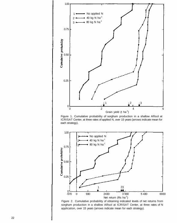
To illustrate, suppose a sorghum crop was grown at, for example, three rates ofnitrogen (0, 40, and 80 kg ha-1) applied as urea on a shallow Alfisol at ICRISATCenter with 15 years of generated daily weather data. To evaluate the various strate-gies, the RA routine sorts the outputs for each strategy into ascending order and thenassigns a probability to each outcome based on the number of years of simulation. Theprobability of any given outcome in a 15-year simulation is 1 /15. From the output andprobability information, a simplified linear segmented approximation to a cumulativeprobability density function (CPDF) can be assembled for each strategy (Fig. 1).

Strategies can be evaluated either in yield or monetary terms. In both cases, themeans and variances associated with each strategy are presented to the user, as is a plotof the CPDFs. The RA package guides the user through identification of the mostappropriate strategy. From CPDFs, the least appropriate strategy based on grainsorghum yield is strategy 1 The most preferred strategy for maximizing yield (furthestto the right) is strategy 3 (80 kg N ha-1).

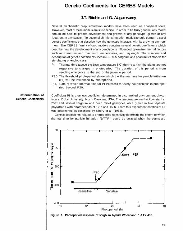
When strategies are to be evaluated in monetary terms, the RA package utilizes theprinciples of stochastic dominance to identify the most "risk efficient" set of strategies.This form of the analysis is used when there is no clear distinction among strategiesfrom the plotted CPDFs (Fig. 2). In monetary terms, strategy 1 is again the leastpreferred because the net return (Rs ha-1) in all years is lowest. However, neither firstorder nor second order stochastic dominance analysis can distinguish between strate-gies 2. and 3. In such cases strategy 2 is chosen by risk preferrers while strategy 3 isselected by decision makers with medium or high aversion to risk. The latter groupprefers strategy 3 over strategy 2 despite the lower mean net return (3620 vs. 3750 Rsha-1) because the medium and high risk-averse groups prefer a more stable strategy,that is one with lower standard deviation (1200 vs 1850 Rs ha-1).

The risk analysis package can also be used to select strategies which deal with theminimums—to minimize stresses during crop growth, minimize nitrogen losses, etc.

21

-570 0 930 2430 3 930 5 430 6930Net return (Rs ha-1)

Figure 2. Cumulative probability of obtaining indicated levels of net returns fromsorghum production in a shallow Alfisol at ICRISAT Center, at three rates of N application, over 15 years (arrows indicate mean for each strategy).

1 23

0

0.25

0.50

No applied N

40 kg N ha-1

80 kg N ha-1

1

2

30.75

1.00

0 2 4 6 Grain yield (t ha-1)

Figure 1. Cumulative probability of sorghum production in a shallow Alfisol atICRISAT Center, at three rates of applied N, over 15 years (arrows indicate mean foreach strategy).

01 2 3

0.25

0.50

0.75

No applied N

40 kg N ha-1

80 kg N ha-1

1

2

3

1.00

22

Discussion

The presentation was complemented by a case study indicating that the choice oftechnique was not critical to substantive issues involving risk assessment. Alternativetechniques, such as mean-variance analysis, the extended mean Gini, stochasticdominance, stochastic dominance with respect to a function, and the expected utilitymoment generating function, gave the same ranking of alternative actions. Therefore,there were diminishing returns to increasing sophistication in risk assessment and thepresent emphasis (in the model) on stochastic dominance was appropriate.

Two suggestions were offered to improve the economic component of the riskassessment routine in the model. First, the output price should be the field price of thecrop standing at harvest. If wholesale prices were used, the results would be biasedagainst the lower yielding strategies. Alternatively, the costs of harvesting, threshing.transport, and marketing could be added to the fixed cost entry in the routine. Second,the risk-neutral, profit-maximizing strategy should be included in the last part of theroutine which lists the optimal choice for a risk-preferring farmer, a slightly risk-averse farmer, a moderately risk-averse farmer, and a severely risk-averse farmer.

23

Thermal Time Estimation

Organization ofDevelopmental Stages

24

Physiology of Sorghum

and Pearl Millet

Simulation of Sorghum and Pearl MilletPhenology

J.T. Ritchie and G. Alagarswamy

Genetic variations in the phenology of plants offer a choice of cultivars to fit diversegrowing conditions. Dynamic modeling requires predictive functions to simulate theduration of various crop growth stages. Such a general phenology model will be a powerful tool in the breeding of new cultivars to fit the length of growing period.

Temperature affects the rate of several developmental processes. Below a certainminimum temperature, no plant development occurs, and above some optimumtemperature, plant development decreases drastically. Between these two definedtemperatures, the plant development rate increases linearly with the increase intemperature. Daily progression of plant development can be precisely described by thegrowing degree day approach.

Several sorghum genotypes in growth chambers were scored for leaf tip appearanceas an indicator of the state of plant development at temperatures ranging from 11 to40° C. Leaf appearance rate was zero at 8°C, which was desi gnated as base tempera-ture (TBASE). Beyond 34° C, leaf tip appearance rates dec lined drastically. Betweenthese limits leaf tips appeared as a linear function of temperature. These results wereused to calculate daily thermal time (DTT) accumulation. When the daily minimumtemperature (TEMPMN) is above TBASE and daily maximum temperature(TEMPMX) is below 34° C, DTT in the model is calculate d as:

DTT = (TEMPMX + TEMPMN) / 2.0 - TBASE (1)

Where T E M P M N is less than TBASE, and T E M P M X is greater than 34°C, a different method is followed to calculate DTT. Accumulated thermal time is the sumof daily DTT values. The cumulative DTT is used to determine the duration of variousphenological stages and to drive the model through time.

Phasic development in the CERES-Sorghum model describes the duration of severalgrowth stages. Organization of growth stages strictly follows the dynamic nature inwhich the plant allocates assimilates to various organs. Growth stages in the model arenumerically coded to route the control through the major growth and phenologysubroutines of the model. Various plant organs actively grow between stages 1 and 5.Stages 7 through 9 are used to describe events occurring during sowing to seedlingemergence. These are important but have a minor effect on phenology. Thereforethese are not discussed in detail.

Stage 1. Seedling emergence to end of juvenile stage. Plants grow vegetatively andproduce leaf primordia during this stage. The rate of development is controlled bytemperature. Since plants are not sensitive to photoperiod in this stage, it is importantto know when this stage is completed in order to implement photoperiod sensitivityrelationships. The genetic differences in the duration of this period are accounted forin the model by a genotype-specific coefficient, P1. The juvenile stage ends when thecumulative DTT equals or exceeds the value of P1.

Stage 2. End of juvenile stage to end of panicle initiation (PI). Plants still produceleaf primordia. At the end of this stage, cellular activity in the apical meristem changesfrom the production of leaf primordia into floral primordia. The rate of developmentis strictly controlled by favorable photoperiod. Since sorghum plants exhibit quantita-tive short photoperiod response, daylengths longer than 12 h delay development.Daylength and photoperiod sensitivity of genotypes determine the duration of thisstage.

The daylength (HRLT) is calculated as a function of solar declination (DEC inradians), sine and cosine of latitude (LAT) and angle of sun at civil twilight. DEC is a sine function of the day of the year (JDATE). Thermal time from seedling emergenceto P1 could be expressed in two photoperiod response ranges, insensitive and sensitive.

In the insensitive range, changes in daylength have no effect on thermal time for PI(DTTPI). There is a threshold photoperiod (P20) above which DTTPI increaseslinearly with increasing photoperiod. The slope (DTTPI per hour increase in day-length) is termed the photoperiod sensitivity coefficient (P2R). The duration of thisstage is dependent upon daylength above P20 and P2R.

Stage 3. Panicle initiation to end of leaf growth. The duration of this stage is from PIuntil flag leaf expansion, and is again temperature dependent. Leaf appearance andexpansion is completed during this stage. Stem growth starts in the earlier part of thisstage and with time exceeds leaf growth rate. This stage is completed when cumulativeDTT equals or exceeds the genetic coefficient P3. The magnitude of P3 was deter-mined from the phenology data reported by Scheaffer (1980). In this study thermaltime for flowering (DTTAN) was directly related to DTTPI.

DTTAN = 1.199 * DTTPI + 450.0 (2)

Since DTTAN is composed of DTTPI and thermal time to reach flowering afterPI (DTTPD), equation 2 can also be written as:

DTTPI + DTTPD = 1.199 * DTTPI + 450.0 (3)

DTTPD could be estimated from equation 3:

DTTPD = 0.199 * DTTPI + 450.0 (4)

The thermal time from flag leaf expansion until flowering in several sorghumgenotypes was estimated to be 150 degree days (Luebbe 1977). After accounting forthis from the thermal time value 450.0 in equation 4, thermal time for completing theleaf development (P3) could be estimated by:

P3 =0.199 * DTTPI + 300.0 (5)

Stage 4. End of leaf growth to beginning of grain filling. During this stage thepanicle develops rapidly and the peduncle grows fast, extending the panicle throughthe flag leaf sheath. Duration of this stage is 270 degree days, and flowering occursafter 150 degree days.

Stage 5. Effective grain filling to physiological maturit y. Thermal time to completethis stage is determined by the genetic coefficient P5. The panicle accumulates most ofthe assimilates because grains are growing rapidly. Even though considerable varia-tion for the duration of grain growth exists among genotypes, most of the commonlygrown genotypes require about 550 degree days to reach physiological maturity.

Stage 6. Physiological maturity to harvest. This stage is reserved for specific userswho may want to simulate possible yield reductions arising from the inability toharvest the crop in time.

25

26

Model Validation

References

180 220 260 100Observed data (day of year)

Figure 1 Comparison of phenology predictions of CFRES Sorg hum model withobserved data from six locations in India

Before the model can be widely used it needs to be adequately tested with independentdata sets The accuracy of predicting phenology is very important since assimilateallocation to different parts of the plant is entirely dependent upon the type of plantorgans that grow in any particular growth stage The phenology predictions weretested using two independent data sets from widely different sorghum-growing regionsof India and USA

Actual and modeled phenological stages for a single hybrid from a range oflocations in India are given in Figure 1 The data set was from a multilocationalmodeling experiment (Huda 1987) in which sorghum hybrid CSH I was grown atseveral locations in India (latitudes 11 31 °N) Data prese nted here indicate that themodel is capable of simulating phenological stages reasonably well The model hasalso been validated using sorghum data from Texas USA

Huda, A.K S. 1987 Simulating yields of sorghum and pearl millet in the semi-aridtropics Field Crops Research 15 309-325

Luebbe, W D 1977 Development events in grain sorghum (Sorghum buolor (L ) Moench) Ph D thesis, Colorado State University Fort Collins Colorado USA

Schaeffer, J.A. 980 The effect of planting date and environment on the phenology andmodeling of grain sorghum Sorghum buolor (L ) Moench P h D thesis Kansas StateUniversity, Manhattan, Kansas, USA

Determination ofGenetic Coefficients

Genetic Coefficients for CERES Models

J.T. Ritchie and G. Alagarswamy

Several mechanistic crop simulation models have been used as analytical tools.However, most of these models are site-specific. In order to be truly generic, any modelshould be able to predict development and growth of any genotype, grown at anylocation, in any season. To accomplish this, simulation models should contain a set ofgenetic coefficients that describe how the genotype interacts with its growing environ-ment. The CERES family of crop models contains several genetic coefficients whichdescribe how the development of any genotype is influenced by environmental factorssuch as minimum and maximum temperatures, and daylength. The numbers anddescription of genetic coefficients used in CERES sorghum and pearl millet models forsimulating phenology are:PI Thermal time (above the base temperature 8°C) during w hich the plants are not

responsive to changes in photoperiod. The duration of this period is fromseedling emergence to the end of the juvenile period.

P20 The threshold photoperiod above which the thermal time for panicle initiation(PI) will be influenced by photoperiod.

P2R Rate at which thermal time for PI increases for every hour increase in photope-riod beyond P20.

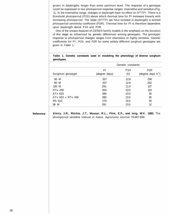
Coefficient PI is a genetic coefficient determined in a controlled environment phyto-tron at Duke University, North Carolina, USA. The temperature was kept constant at25°C and several sorghum and pearl millet genotypes wer e grown in two separatephytotrons with photoperiods of 12 h and 15 h. From this experiment coefficient PIwas determined as described by Kiniry et al. (1983).

Genetic coefficients related to photoperiod sensitivity determine the extent to whichthermal time for panicle initiation (DTTPI) could be delayed when the plants are

600

550

500

450

Insensitive Sensitive

P20

40010 12 14 16 18

Photoperiod (h)

Figure 1. Photoperiod response of sorghum hybrid Wheatla nd * ATx 430.

27

Reference

28

grown in daylengths longer than some optimum level. The response of a genotypecould be expressed in two photoperiod response ranges: insensitive and sensitive (Fig.1). In the insensitive range, changes in daylength have no effect on DTTPI . There is a threshold photoperiod (P20) above which thermal time for PI increases linearly withincreasing photoperiod. The slope (DTTPI per hour increase in daylength) is termedphotoperiod sensitivity coefficient (P2R). Thermal time for PI is therefore dependentupon daylength above P20 and P2R.

One of the unique features of CERES family models is the emphasis on the durationof this stage as influenced by genetic differences among genotypes. The genotypicresponse to photoperiod changes ranges from insensitive to highly sensitive. Geneticcoefficients for P I , P20, and P2R for some widely different sorghum genotypes aregiven in Table 1.

Table 1. Genetic constants used in modeling the phenology o f diverse sorghumgenotypes.

Genetic constants

PI P20 P2RSorghum genotype (degree days) (h) (degree days h-1)

60 M 337 12.8 29080 M 337 12.6 262

100 M 291 11.0 127RTx 430 400 13.0 123ATx 623 380 13.0 35ATx 623 x RTx 430 390 13.0 35RS 610 275 15.5 3038 M 291 13.0 12

Kiniry, J.R., Ritchie, J.T., Musser, R.L., Flint, E.P ., and Iwig, W X . 1983. Thephotoperiod sensitive interval in maize. Agronomy Journal 75:687-690.

Discussion

Several participants were concerned about the effect of nutrient and drought stresseson crop phenology. The speakers felt that these were of importance only under'extreme' stress levels. Mild drought stress hastened flowering since the meristemtemperature increased, but severe stress levels delayed flowering. At this stage it is notpractical to incorporate these in the phenology subroutine. The chairman also pointedout the difficulty of separating individual and combined efforts of nutrients and wateron sorghum genotypes.

A participant asked whether it is practical to generate genotype-specific coefficientscontinuously to predict phenology because newer cultivars are regularly released. Itwas pointed out that on the basis of a line x tester study, the phenology of the hybridcould be predicted from that of the female parent.

The possibility of drawing inferences on weather-based crop phenological data wasquestioned. It was generally felt that this was only possible in gross terms. The effect ofextreme temperature (low and high) on phenology was discussed. It was felt that thegenotype differences were mostly in terms of survival rather than in the rates ofdevelopment. Genotypes tolerant to cold may not necessarily be able to tolerateextremely high temperatures. Generally it was felt that additional input data such ascanopy and soil temperatures, and soil moisture content for improving the precision ofphenological predictions would unnecessarily complicate the models.

To a specific query on genotype coefficients of millets, it was stated that experiencewith 10 pearl millet genotypes was similar to that of sorghum.

On the relative importance of photoperiod before and after panicle initiation, thespeakers clarified that photoperiod directly influences phenology only before panicleinitiation. Later effects are mere reflections of the additional time needed for expand-ing leaves for which primordia were laid before panicle initiation.

One question related to the effect of the same mean temperature with varyingmaximum and minimum values. It was felt that within the linear range of phenologicalresponse (8 34° C), the mean value sufficiently reflected the effect of maximum andminimum temperatures. When it was pointed out that genotypic differences in basetemperatures for seed germination are substantial, the speaker felt that thermal timefor leaf tip appearance is conservative and probably unrelated to that based ongermination. On thermosensitivity, the speaker suggested that 'thermosensitivity* maybe attributed to vernalization requirement and expressed the need for consideration oftemperature during floral induction period.

The discussion closed with remarks on the wider application of simple models topredict phenology, and encouraged participants to collect relatively simple data over a wider range of environments to increase the application of the models. Efforts shouldalso be made to relate shoot phenology to root phenology and growth.

29

Modeling Sorghum and Pearl Millet

RESCAP: A Resource Capture Model forSorghum and Pearl Millet

J.L. Monteith, A.K.S. Huda, and D. Midya

Two processes dominate most contemporary models of crop growth: resource captureand the distribution of metabolites to organs with different functions. In field andlaboratory studies which provide information for models, most attention has focused

• the role of photosynthesis as determined by radiation, C02 , temperature, leaf waterstatus, etc.; and

• water uptake by roots as determined by the balance between atmospheric"demand" and soil "supply."

Radiation Rain Stored water

Leaf areaSoil

evaporation

Root lengthdensity

Drainage

PotentialDMP SMD

Supply

Potentialextraction

WUE

supply > SMDIf

supply = SMDand

POT.T > POT XT

IfWUE

ActualDMP

Potentialtranspiration

Partitioning

Leaves Roots

Structures

Reproductive organs

Figure 1. Flow diagram of the RESCAP model.

30

Light Interception andDry Matter Production

Much less attention has been paid to the plant factors that determine watersupply —the size of the root system, and the rate at which roots move into new soil.

A new resource capture model, RESCAP, places equal emphasis on the role ofleaves in relation to the interception of light, and to the role of roots in relation to theuptake of water (Fig. 1). Two assumptions, which are well supported by field evidence,are central to the model (Monteith, in press):• the amount of dry matter produced per unit of radiation intercepted by foliage is

effectively constant during vegetative growth when water is not limiting; and• the amount of dry matter produced per unit of water transpired is inversely

proportional to mean saturation deficit constant whether water is limiting or not.Building a model around these conservative quantities keeps the structure simple

and is equivalent to the use of constants in physical models, e.g., gravitationalacceleration in the relation between the length and period of oscillation of a pendulum.

RESCAP was developed primarily to predict the growth and yield of sorghum andpearl millet, given an appropriate set of environmental variables and genetic coeffi-cients. However, it could readily be adapted to any cereal, and indeed to any seed-producing crop. For sorghum, genetic coefficients are available from measurements atICRISAT Center and elsewhere.

At all stages of growth, the rate of dry matter production C (kg m-2 d-1) per unit ofintercepted solar radiation S (MJ m-2 d-1) is assumed to have a constant value e provided water is not limiting.

Thus if q is the mass of dry matter produced per unit mass of water transpired, andSD is the mean saturation deficit of the atmosphere (kPa), the quantity qD = q x SD isconservative for most crops and has a value of about 9 g kg-1 kPa for C4 cereals(Monteith 1989). The value of q in kg dry matter per kg water is therefore 9 x I0 - 3 /SD.

On a day when dry matter production is C, the demand for water to transpire isC*SD/ (qD) . If this quantity is less than the amount of water which the roots cansupply (estimation described later), then growth is assumed to be light-limited and hasthe value:

C = f i e S (1)wherefi is the fraction of radiation intercepted by foliage as estimated by the conventionalrelation

f i = 1 - exp (-KL) (2)whereL = leaf area indexK = extinction coefficient.

The leaf area index is augmented each day by the increase (dL) calculated as theincrease in dry weight C multiplied by the leaf area ratio D, i.e.,

dL = D * C (3)

The leaf area ratio (m2 leaf per g plant) is calculated as:

D = B (1 - xr - xst)where

B = specific leaf area (m2 leaf per g leaf)xr = fraction of dry matter allocated to roots

xst = fraction of dry matter allocated to stems.

B is assumed constant at 33.0 m2 kg-1 in the current version of the model.

31

Extraction of Water: Roots

Water Capture

32

The volume of available water per unit volume of soil AW is assumed to be a functionof depth z and the initialization of this quantity is discussed in the next section.

The size and distribution of the root system is specified by two parameters: thedownward velocity of a root "front" called THCK (thickness of layer penetrated in oneday) and the root length per unit volume RLV (m length per m3 of soil).

Using a neutron probe we found that the velocity of the root front achieved bysorghum reached a maximum value R R M A X of about 0.035 m d-1 about 20-30 daysafter emergence (Monteith 1986). We assumed that the effective root front movesdown at the same rate, recognizing that roots penetrate below the depth at which theextraction of water can be detected.

Field measurements on sorghum and pearl millet at ICRISAT Center show thatRLV usually has a maximum value of 1 to 2 * 104 m m-3 at minimum root depth(RDMIN) and decreases with depth to about 1/10 of this range at a maximum rootdepth ( R D M A X ) at approximately 2 m. We assume that RLV is inversely propor-tional to the square root of rooting depth RD. Then RLV at depth RD is:

RLV(RD) = RLV( l ) * ( R D M I N / R D ) 0 . 5 (4)

As the allocation of dry matter to the root system is a fraction xr of C then

xr * C (TIME) = RHO * RLV * THCK (TIME) (5)whereRHO is root weight per unit length (kg m-1).

During early growth, we used equation 5 to calculate THCK, setting xr at anarbitrary value of 0.3. When THCK reached its maximum value of R R M A X , we setTHCK at R R M A X and allowed xr to decrease with increasing depth.

Provided there is no rain or irrigation and evaporation is limited by water extractionand not by water demand, the available water at depth z and time t' is assumed todecrease exponentially with time:

AW(z,t') = AW(z,o) * exp (-t' / TAU) (6)where

t' = time when the rooting front arrives at depth z, andTAU = time constant for the extraction process.

Field measurements on sorghum gave values in the range 20-100 days decreasingwith depth. We assume that TAU is inversely proportional to the root length density assuggested by Passioura (1983) so that TAU is proportional to the square root of depth.The rate of extraction at any depth is:

- d [AW(z,t')] / dt = [AW(z,o) / TAU] * exp (-t' / TAU) (7)

The depth of the layer traversed by the root zone on the day defined by time t afteremergence is THCK so that the amount of water extracted from the layer is:

THCK * d [AW(z,t')] / dt' (8)

The total potential extraction XT for the whole profile on day t is summed for valuesof t' from 1 to t (step 1). If XT is less than the water equivalent of dry matter productionas estimated from light interception, XT is adopted as the transpiration rate and therate of dry matter production becomes:

C = (qD/D) * XT (9)

If the layer of soil above the drying front but below seed depth is wetted by rain orirrigation, we assume that growth and transpiration are light-limited until this waterhas been removed. The rate of transpiration then reverts to XT if demand exceedssupply. The criterion for the switch from light-limited to water-limited growth isestablished in the following section.

Evaporation fromSoil Surface

Soil Water Status

Water Budgets

Criterion for Water-LimitedGrowth and Transpiration

Phenology

To estimate evaporation from the soil, we used a bucket model and assumed that thedepth of the bucket was equal to the depth of sowing. Below this depth, the rate ofdiffusion to the soil surface was assumed negligible compared with the rate ofextraction by the root system.

The rate of evaporation Es from newly wet soil with no ground cover was assumedto be 0.9 times the rate of evaporation from a Class A pan, (EP). Ground coverreduced the rate by the factor of (1 - f i). Drying reduced the ratio by a factor equal tothe amount of water in the surface layer expressed as a fraction of water held at fieldcapacity. If AW is the actual water content of the layer, AD is the air-dry value and FCis the water content at field capacity:

Es = 0.9 * (1 - f i) * (AW - AD) / (FC - AD) (10)

The air-dry water content was assumed to be one-third of the value at 1.5 MPa.

At R D M A X , taken as 2 m, the maximum available water content (MAW) in both theVertisol and the Alfisol at ICR1S AT Center is assumed to be half the value at 0.1 m. Toinitiate the distribution of water, the ratio of actual to maximum available water ISWis assumed to have the same value at all depths. The decrease of available water withdepth is:

AW = MAW * (1 - 0.5 * RD / R D M A X ) * ISW (11)

The corresponding initial soil water deficit (mm) is:

SMDO = 0.75 * MAW * (1 - ISW) * (RDMAX - RDMIN) * 1000 (12)

Changes in the soil moisture deficit of the surface layer (0.1 m deep) occur as a result ofthe direct input of water from precipitation (P) or irrigation (IRR) and losses as a consequence of evaporation (E) or percolation (PRC). Suppose SM 10D is the soilwater deficit at the beginning of day t.

If (P + IRR) > SM10D,

then PRC = P + IRR - SM 10D, and SM 10D = 0.

But if P + IRR SM 10D then PRC = 0 and SM10D = SM 10D - (P + IRR)

Similar algorithms are used if the soil moisture deficit (SMD) in the root zoneincreases as a result of percolation from above (PRC) and decreases as a result oftranspiration (T) and drainage (DR). In this case, the loss of water from the bottom ofthe layer becomes the drainage component DR.

A central feature of the model is the comparison each day between the accumulatedextractablc water SXT and SMD - SMDO, which is the net decrease of soil watercontent since the start of growth. When SXT < SMD - SMDO, the rate of wateruptake by the root system is assumed to be limited by equation 8 which is applied eachday throughout the root zone. In this case, the rate of transpiration and of growth areboth treated as water-limited. Conversely, if SMD - SMDO is less than SXT becauseof an input of water from rain or irrigation, the difference between SXT and SMD istreated as an amount of (free) water which can be supplied by the root system asrapidly as it is demanded by the shoots. This demand is determined by the daily drymatter production and the value for the dry matter water ratio.

The phenological timetable was divided into the usual three stages: GS1 from emer-gence to panicle initiation, GS2 from panicle initiation to anthesis, and GS3 fromanthesis to maturity. The length of each stage is specified in terms of thermal time(units of degree days) above a base of 7° C and daylength . The daily mean temperaturewas assumed to be the average of reported maximum (Tmax), and minimum tempera-

33

Allocation of Dry Matterto Shoots

References

Leaf Area Development

34

tures (1 min), except when T max exceeded 38° C, in which case it was assigned a valueof 38° C (Huda 1987). The influence of daylength on deve lopment rate is allowed forwhere appropriate.

The fraction of above-ground dry matter is divided between leaves (FL), stem (FS),and grain (FG) in proportions which change with plant age.

From emergence to the end of GS2, FL decreases from 0.9 to 0.1 and FS increasesfrom 0.1 to 0.9. During the first 6 days of GS3, both FL and FS decrease to zero andFG increases from zero to unity, remaining at 1 till the end of GS3.

In an alternative procedure for calculating yield, grain number is assumed propor-tional to the increase of total plant weight in GS2. Weight per grain (W) is thenassumed proportional to the length of GS3 and the total dry weight at the end of GS3.In this case, the harvest index is simply proportional to the length of GS3. However, ifG W calculated in this way exceeds a limiting maximum value of 0.035 g, it is assignedthat value. The effect of this restriction is that harvest index is smaller when vegetativegrowth is very vigorous.

Huda, A.K.S. 1987. Simulating yields of sorghum and pearl millet in the semi-aridtropics. Field Crops Research 15:309-325.

Monteith, J.L. 1986. How do crops manipulate water supply and demand? Philoso-phical Transactions of the Royal Society A 316:245-259.

Monteith, J.L. (In press.). Steps in crop climatology. In Proceedings of the Interna-tional Conference on Dryland Farming. 15-19 Aug 1988, Amarillo, Texas, USA.(Unger, P.W., Jordan, W.R., Sneed, T., and Jensen, R.W., eds.). College Station,Texas, USA: Texas A & M University.

Passioura, J.B. 1983. Roots and drought resistance. Agricultural Water Management7:265-280.

Simulation of Growth and Development inCERES Models

J.T. Ritchie and G. Alagarswamy

Potential productivity of a crop generally depends on conservation of solar energythrough photosynthesis when other limiting factors are absent. Only the wavelengthbands from 0.4-0.7 m are useful, a range known as photosynthetically active radia-tion (PAR). Potential productivity depends on how much of the PAR is intercepted bythe crop canopy. Therefore, relating crop growth to PAR interception by the canopyhas been more successful than conventional growth analysis. This paper is confined tosimulation of growth because developmental aspects have been dealt with earlier inthis volume.

Accurate prediction of leaf area depends on the ability to predict leaf appearance rate.If temperature records are available, the number of leaves that appear can be calcu-lated using the leaf appearance interval (PHINT). The PHINT values (in degree daysper leaf) are 49 for sorghum and 43 for pearl millet.

Assimilate Production

Assimilate Allocation

Since leaves appear only in growth stages 1 to 3, the cumulative number of fullyexpanded leaves (CUMPH) in sorghum is calculated from the daily thermal time(DTT):

CUMPH = CUMPH * DTT / PHINT (1)

Cumulative leaf area of the plant on a given day is then calculated using theGompertz function:

(-K * CUMPH)(be)

PLAN = Ae (2)wherePLAN = cumulative leaf area

A = maximum leaf area at infinite timeb,K = constants

Individual leaf size of sorghum genotypes differs widely, leading to very differentcumulative leaf area. Among narrow- and broader-leaved genotypes the constant K inthe Gompertz function varied to a greater extent (25%) compared to the constant b (2%). Hence constant K could be a genotype-specific coefficient.

Leaf expansion growth is sensitive to unfavorable temperatures and soil waterdeficit. The optimum temperature for maximum leaf expansion for 25 sorghumgenotypes ranged between 14 and 32°C in a controlled grow th chamber study (Rit-chie, J.T. and Alagarswamy, G., unpublished).

The input variable solar radiation (SOLRAD) is first converted into PAR. Therelative amount of transmitted light within any crop canopy decreases exponentiallyas described by the Bouger-Larnbert law. Using this law the amount of light inter-cepted (1/I<>) by the canopy is calculated as:

I / I 0 = e ( - K * L A I ) (3)where

K = extinction coefficientLA I = leaf area index

Thus 1/10 is generally influenced by K and LAI . In the model, values of K decreasenonlinearly as row spacing increases. Once the amount of PAR intercepted(INTPAR) by the crop canopy is computed, potential daily biomass production(PCARB) is calculated:

PCARB = 4.0 * INTPAR (4)

It is assumed that 4.0 g of total biomass (including roots) are produced for every M J of PAR intercepted. The expansive and leaky root systems of crops are likely to looseabout 35-45% of assimilates partitioned to the roots into the surrounding soil as rootexudates. To compensate for such large losses, a higher efficiency of conversion factoris used in the model.

The actual biomass produced is generally well below the potential amount becauseboth biotic and abiotic factors reduce the potential amount. Therefore, in the modelpotential biomass production is constrained by non-optimal temperature factor(PRFT), nitrogen deficiency factor, and water deficit (SWDF1) factors. Values forthese factors range from zero to unity.

In the model the optimum temperature range for photosynthesis was set between 20and 40° C. When day temperatures deviate from this range, PRFT is used to reduce therate of photosynthesis.

Stage 1. Leaves and roots constitute the growing organs. Leaf area growth rate(PLAG) is converted to mass growth rate (GROLF) using specific leaf weight (SLW).

35

36

The remainder of the daily assimilate supply (CARBO) is allocated to the root growth(GRORT). If GRORT is less than 25% of CARBO, then GROLF is reduced to 75% ofCARBO and the rest is allocated to roots.

Stage 2. Leaves and roots continue to be the major growing o rgans. In some casesthe stem also starts to grow and is about 10% of leaf growth. Root growth is neverallowed to fall below 25% of CARBO.

Stage 3. Leaves, stems, and roots are the major growing o rgans. Leaf growth iscompleted now. Leaf weight is derived from PLAG using specific leaf weight. Stemgrowth increases linearly with DTT. Minimum value for GRORT is set at 30% ofCARBO. If GRORT values fall below the minimum value, growth of other organs isreduced to set GRORT at the minimum value. Finally STMWT, LFWT, and PLAvalues are updated.

Stage 4. Stem, panicles, and roots are the major growing parts. Since it is not knownwhen the major portion of panicle growth started, weights of panicle and stem arecombined. GROSTM is a linear function of thermal time and influenced by theminimum of two stress factors.

GROSTM = 0.07 * DTT * AMIN1 (SVVDF2, TEMF) (5)

The root growth consists of the remainder of CARBO. GRORT is set to a minimumof 20% of CARBO. Leaf senescence due to normal development becomes a majorcause of reduction in leaf area. It is calculated as a nonlinear function of DTT.

Stage 5. Panicles are the major growing organ. As stated earlier, panicles are growndaily as an integral part of stem weight (STMWT). On the first day in this stage panicleweight (PANWT) is calculated. From then on panicles are grown as independentorgans.

PANWT = 0.3 * STMWT (6)

The rate of biomass production during stage 5 is generally lower than in earlierstages. Post-anthesis decline in the efficiency of conversion is accounted for in themodel by reducing the calculated value of CARBO.

The sorghum panicle has primary, secondary, and tertiary branches, and grainsdevelop in each branch. This causes an enormous difference in grain size within thepanicle. Thus, unlike CERES Wheat and Maize models, growth rate of the wholepanicle (GROPAN) is modeled in sorghum rather than individual grains.

The optimum mean temperature for grain growth in sorghum varies from 20 to25° C. Kernel weight is markedly reduced beyond this range. Hence in modelingpanicle growth, a relative panicle filling rate (RGFILL) is calculated first as a functionof temperature. RGFILL is proportional to temperature and its value ranges fromzero to unity. When T E M P M N is between 20 and 25°C, the va lue for RGFILL isunity. For T E M P M N values beyond this range, RGFILL is reduced linearly to zero.Panicle size at the time of anthesis influences the rate of its growth during grain filling.Panicle growth constant (PGC) accounts for the influence of panicle size on its rate ofgrowth.

As the panicles approach physiological maturity, their growth rate slows down andis accounted for by a panicle aging factor (PAF). When there is a water deficit,SWDF2 is used to reduce the GROPAN.

GROPAN = RGFILL * PGC * PAF * SWDF2 (7)

If all the CARBO is not utilized to support GROPAN, which happens underadequate moisture, the remainder of CARBO is equally partitioned to grow stems androots. Under severe water deficit, stored materials from the stem are known to support

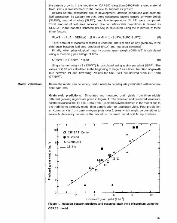
Model Validation

the panicle growth. In the model when CARBO is less than GROPAN, stored materialfrom stems is translocated to the panicle to support its growth.

Besides normal senescence due to development, adverse conditions also promoteleaf senescence. To account for this, three senescence factors caused by water deficit(SLFW), mutual shading (SLFC), and low temperature (SLFT) were computed.Total amount of leaf area senesced due to unfavorable conditions is termed asSENLA. Plant leaf area senesced (PLAS) is calculated using the minimum of thesethree factors:

PLAS = (PLA - SENLA) * [1.0 - A M I N 1 (SLFW,SLFC,SLFT)] (8)

Total amount of leaf area senesced is updated. The leaf area on any given day is thedifference between leaf area produced (PLA) and leaf area senesced.

Finally, when physiological maturity occurs, grain weight (GRNWT) is calculatedusing a threshing percentage of 80%.

GRNWT = PANWT * 0.80 (9)

Single kernel weight (SKERWT) is calculated using grains per plant (GPP). Thevalues of GPP are calculated in the beginning of stage 5 as a linear function of growthrate between PI and flowering. Values for SKERWT are derived from GPP andGRNWT.

Before the model can be widely used it needs to be adequately validated with indepen-dent data sets.

Grain yield predictions. Simulated and measured grain yields from three widelydifferent growing regions are given in Figure 1. The observed and predicted values arescattered close to the 1:1 line. Data from Bushland is overestimated in the model due tothe inability to correctly model tiller contribution to total grain yield. Poor predictionat Kununurra is from zero nitrogen plots over 2 years which might be due either tosevere N deficiency factors in the model, or incorrect initial soil N input values.

10

8

6

4

2

0

ICRISAT Center

Bushland

Kununurra

1:1 line

0 2 4 6 8 10

Observed grain yield (t ha-1)

Figure I. Relation between predicted and observed grain y ield of sorghum using the

CERES model.

37

N Response. Location specificity of grain yield response to N fertilizer was testedusing data from ICRISAT Center (Fig. 2). At ICRISAT Center over the range of 0 to160 kg N ha-1, the model predicted the N response reasonably well. However modelpredictions in Kununurra where the N level ranged from 0 to 370 kg ha-1, were not verygood. The model did not simulate N response at lower and higher N levels.

38

ObservedPredicted

6

4

2

00 40 80 120 160

Nitrogen rate (kg ha-1)

Figure 2. Relation between observed and predicted grain y ield of sorghum over a range of N levels.

Discussion

During the discussion on the RESCAP model it was clarified that the model assumesonly three layers of soil: 0-10 cm, 10 cm to root front (maximum depth of descendingroots), and below the root front. Root senescence is not considered. The model has nonutrient subroutine at present and is applicable only where nutrients are not limiting.It was mentioned that the lack of fit for sorghum cultivar CSH 6 in the postrainyseason could be due to its temperature sensitivity. This could be easily tested byaltering the TBASE.

There was some concern expressed as to why the model, which was to predict totalbiomass more elegantly, poorly predicted biomass compared to grain yields. Someconcern was also voiced regarding the use of the same data for model building andmodel testing. A question on the philosophy of no carbon allocation to roots afteranthesis was raised. It was clarified that roots remain functional but do not grow afteranthesis. On the question of the simple RESCAP model requiring more weatherparameters than the CERES model, it was mentioned that the authors were trying toreduce this requirement, but felt that the saturation deficit parameter was essential. Itwas also suggested that the model be validated by estimating biomass by growth stagessince data for such analyses were available. On the question of whether such modelscould be used in remote sensing, the authors replied that it could be done with somemodifications.

In the discussion following the presentation of simulation of growth and develop-ment in CERES models, clarification was sought regarding the calculation of poten-tial leaf area from the number of leaves, leaf size, etc. It was suggested that sink sizealso determined the rate of senescence after anthesis. It was also mentioned that greenleaves do not necessarily constitute functional leaves. Because only the top four or fiveleaves of sorghum contribute most to photosynthesis, the senescence of lower leavesmay not be of consequence, It was clarified that both N and water deficits affectedexpansion growth. It was pointed out that specific leaf area varied with age. UnlikeSORGF, the CERES model is not based on a given leaf number, rather the leafnumber is determined by a genetic constant and photoperiod in GS1.

The potential of such a model for the geographical mapping of crop grain yields wasraised. The authors replied that it could be achieved if variations were only in N andwater. The model does not take into account insect pests, diseases, weeds, phosphor-ous, and other micronutrients.

Queries on the rationale of a single TBASE were raised. It was pointed out thatunlike the TBASE based on germination and emergence, the model uses TBASE andT M A X based on leaf tip appearance. When both SWDF1 and SWDF2 were operat-ing, the law of minimum was applied. It was clarified that when nitrogen was limiting.leaf expansion was affected, but photosynthesis was not affected. The model shouldlook into the compensatory mechanisms operating. It was felt that the tillering routineneeded improvement. Indian sorghums have been bred against tillering, and tilleringwas noticed when temperatures fell below 10°C.

39

Models

Software and Documentation

Reference

Additional Documentation

40

ConclusionModels, Software, and Documentation

J.T. Ritchie, J.L. Monteith, D.C. Godwin, and A.K.S. Huda

The crop models described and discussed were primarily the CERES models series2.00 and the RESCAP model, both of which concentrated on sorghum, and to a lesserextent on pearl millet. Functional models adopted by the IBSNAT project presentlyinclude those on maize, wheat, and soybean, and when sufficiently validated willinclude sorghum, pearl millet, groundnut, potato, barley, and field bean. Revisions inthe CERES models are incorporated every 18 months.

Some important areas for future improvement of the models are:• more detailed treatment of root growth;• better understanding of runoff and infiltration;• tillage aspects and their effect on root environment, water storage in the surface

layer, N-dynamics through residue incorporation;• incorporation of information on ammonia loss;• simulation of phosphorus dynamics;• study of rotational effects and legumes in the system; and• evaporation process and ET aspects.

Although the present version of the DSSAT package is preliminary, it was possible toprovide diskettes and documentation. In fact, a majority of the participants receivedavailable software and documentation. IFDC plans to make available versions of theCERES models with a user manual. A list of documents distributed during theworkshop is provided in the Appendix below. Texas A & M University, USA, haspublished a book on CERES-Maize, (Jones and Kiniry 1986) which comes with twodiskettes. A similar book on CERES-Wheat is likely to be available in mid-1989,followed by one on CERES-Sorghum in 1990.

Jones, C.A., and Kiniry, J.R. 1986. CERES-Maize: A simulation model of maizegrowth and development. College Station, TX, USA: Texas A & M University Press.194 pp.The documentation listed below is available either from the authors or concernedinstitutions.Alagarswamy, G., Ritchie, J., Godwin, D .C , and Singh, U. 1989. A user's guide toCERES-Sorghum, Version 2.00. Honolulu, H I , USA: IBSNAT.IBSNAT (International Benchmark Sites Network for Agrote chnology Transfer).1988. Data base management system, experiment data entry draft user's guide,Version 2.1. Honolulu, H I , USA: IBSNAT.IBSNAT (International Benchmark Sites Network for Agrotec hnology Transfer).1988. Experimental design and data collection procedures for IBSNAT-the minimumdata set for systems analysis and crop simulation. 3rd edn. Technical Report 1.Honolulu, H I , USA: IBSNAT. 74 pp.IBSNAT (International Benchmark Sites Network for Agrote chnology Transfer).1988. Data base management system, MDS retrieval for crop models, draft user'sguide, Version 2.1. Honolulu, H I , USA: IBSNAT.IBSNAT (International Benchmark Sites Network for Agrot echnology Transfer).1988. Data base management system, weather entry data, draft user's guide, Version2.1. Honolulu, H I , USA: IBSNAT.Ritchie, J.T., and Crum, J. 1988. Converting soil survey characterization data intoIBSNAT crop model input. Honolulu, H I , USA: IBSNATMonteith, J.L., Huda, A.K.S., and Midya, D. 1988. RESCAP: a general crop modelbased on process of resource capture, (unpublished.)

Participants

M.R. ChaudharySenior Soil PhysicistDepartment of SoilsPunjab Agricultural UniversityLudhiana 141 004India

Renu K. ChopraPlant PhysiologistWater Technology CentreIndian Agricultural Research InstituteNew Delhi 110 012India

R.G. DumsdaySenior LecturerSchool of AgricultureLa Trobe UniversityBundoora, Victoria 3083Australia

H. EswaranProgram LeaderSoil Management Support ServicesU.S. Department of AgricultureP.O. Box 2890Washington, D.C. 20013USA

D.C. GodwinAgronomist and Systems ModelerInternational Fertilizer Development CenterP.O. Box 2040Muscle Shoals, AL 35662USA

S.S. HundalAgrometeorologistAll India Coordinated Research Projecton Agrometeorology

Department of Agricultural MeteorologyPunjab Agricultural UniversityLudhiana 141 004India

T.N. Ashok KumarAssistant AgronomistAll India Coordinated Research Projectfor Dryland Agriculture

GKVK CampusBangalore 560 065India

A.N. MehtaProfessor and HeadDepartment of Agricultural MeteorologyB.A. College of AgricultureGujarat Agricultural UniversityAnand 388 110India

Abdi Ahmed MohammedUSAID-Wyoming TeamBay Region Agricultural Development ProjectBonka Research StationP.O. Box 2971MogadishuSomalia

R.S. NarangProfessor and HeadDepartment of AgronomyPunjab Agricultural UniversityLudhiana 141 004India

B.S. RanaProject Coordinator (Sorghum)National Research Centre for SorghumRajendranagarHyderabad 500 030India

J.T. RitchieHomer Nowlin ChairDepartment of Crops and SoilsPlant and Soil Science BuildingMichigan State UniversityEast Lansing, MI 48824-1222USA

G.S. SaroaAssistant Soil ChemistDryland Research ProjectPunjab Agricultural UniversityGarshankarHoshiarpur 144 527India

U. SchulthessAgronomistInternational Livestock Centre for AfricaP.O. Box 5689Addis AbabaEthiopia

41

Phool SinghCrop PhysiologistCollege of AgricultureHaryana Agricultural UniversityHisar 125 004India

S.P. SinghProject CoordinatorCentral Research Institute forDryland Agriculture

Santoshnagar, P.O. SaidabadHyderabad 500 659India

Upendra SinghSoil Scientist and Systems ModelerInternational Fertilizer Development CenterP.O. Box 2040Muscle Shoals, AL 35662USA

S.K. SinhaProfessor of EminenceWater Technology CentreIndian Agricultural Research InstituteNew Delhi 110 012India

Chirtchart SmitobolHead, Soil and Water ManagementFarming Systems Research InstituteDepartment of AgricultureBangkhenBangkokThailand

H.L.S. TandonDirectorFertiliser Development and ConsultationOrganization

C-110, Greater Kailash 1 New Delhi 110 048India

M.C. VarshneyaProfessor-in-ChargeCentre for Advanced Studies inAgricultural Meteorology

College of AgriculturePune411 005India

ICRISAT

M. GoonAssistant Director General (Administration)B.C.G. GunasekeraAdvisor to the Director General for Donor RelationsJ.S. KanwarDeputy Director General (Emeritus)J.L. MonteithDirector, Resource Management Program (RMP)Y.L. NeneDirector, Legumes ProgramK.B. SrinivasanAssistant Director General (Liaison)J.M.J, de WetDirector, Cereals ProgramG. AlagarswamyPlant Physiologist I I , CerealsF.R. BidingerPrincipal Plant Physiologist, CerealsJ.R. BurfordPrincipal Soil Chemist, RMPD.R. ButlerPrincipal Microclimatologist, RMPJ.W. EstesComputer Services OfficerL. FlynnSenior Documentation Assistant, Computer ServicesS.D. HallActing Head, Information ServicesA.K.S. HudaAgroclimatologist I I , RMPK.B. LaryeaPrincipal Soil Physicist, RMPK.K. LeePrincipal Cereals Microbiologist, RMPV. MahalakshmiPlant Physiologist I I , CerealsC.K. OngPrincipal Agronomist (Cropping Systems), RMPD.L. OswaltProgram Leader, TrainingJ.M. PeacockPrincipal Plant Physiologist, CerealsT.J. RegoSoil Scientist I I , RMPK.L. SahrawatSr. Soil Scientist I I , RMPN. SeetharamaSr. Plant Physiologist I I , CerealsA.M. ShekhResearch Fellow, RMP

42

Piara SinghSoil Scientist I I , RMPR.P. SinghEconomist I I , RMPSardar SinghSoil Scientist I I , RMPG.D. SmithPrincipal Soil Scientist, RMPD.P. VermaSoil Scientist/Chemist, RMPS.M. VirmaniPrincipal Agroclimatologist, RMPT.S. WalkerPrincipal Economist, RMPS.P. WaniMicrobiologist I I , RMP

43

Glossaries

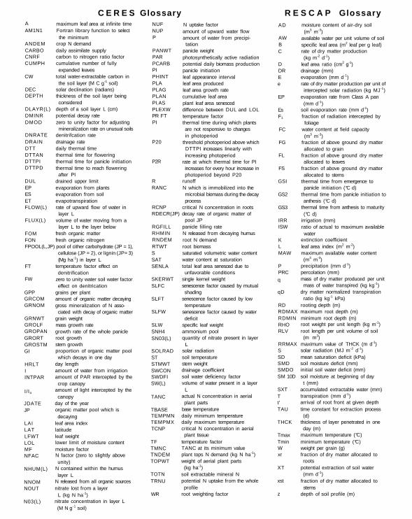
AAM1N1

ANDEMCARBOCNRFCUMPH

CW

DECDEPTH

DLAYR(L)DMINRDMOD

DNRATEDRAINDTTDTTANDTTPIDTTPD

DULEPESETFLOW(L)

FLUX(L)

FOMFON

maximum leaf area at infinite timeFortran library function to selectthe minimum

crop N demanddaily assimilate supplycarbon to nitrogen ratio factorcumulative number of fullyexpanded leaves

total water-extractable carbon inthe soil layer (M C g-1 soil)

solar declination (radians)thickness of the soil layer beingconsidered

depth of a soil layer L (cm)potential decay ratezero to unity factor for adjustingmineralization rate on unusual soils

denitrifcation ratedrainage ratedaily thermal timethermal time for floweringthermal time for panicle initiationthermal time to reach floweringafter PI

drained upper limitevaporation from plantsevaporation from soilevapotranspirationrate of upward flow of water inlayer L

volume of water moving from a layer L to the layer below

fresh organic matterfresh organic nitrogen

FPOOL(L,JP) pool of cither carbohydrate (JP = 1),

FT

FW

GPPGRCOMGRNOM

GRNWTGROLFGROPANGRORTGROSTMGI

HRLTIINTPAR

I/Io

JDATEJP

LAILATLFWTLOLMFNFAC

NHUM(L)

NNOMNOUT

N03(L)

cellulose (JP = 2), or lignin (JP= 3)(Mg ha-1) in layer L

temperature factor effect ondenitrification

zero to unity water soil water factoreffect on denitrication

grains per plantamount of organic matter decayinggross mineralization of N asso-ciated with decay of organic matter

grain weightmass growth rategrowth rate of the whole panicleroot growthstem growthproportion of organic matter poolwhich decays in one day

day lengthamount of water from irrigationamount of PAR intercepted by thecrop canopy

amount of light intercepted by thecanopy

day of the yearorganic matter pool which isdecaying

leaf area indexlatitudeleaf weightlower limit of moisture contentmoisture factorN factor (zero to slightly aboveunity)

N contained within the humuslayer L

N released from all organic sourcesnitrate lost from a layer

L (kg N ha-1)nitrate concentration in layer L (M N g-1 soil)

NUFNUPP

PANWTPARPCARBPIPHINTPLAPLAGPLANPI.ASPLEXWPR FTPI

P20

P2R

RRANC

RCNP

N uptake factoramount of upward water flowamount of water from precipi-tation

panicle weightphotosynthetically active radiationpotential daily biomass productionpanicle initiationleaf appearance intervalleaf area producedleaf area growth ratecumulative leaf areaplant leaf area senesceddifference between DUL and LOLtemperature factorthermal time during which plantsare not responsive to changesin photoperiod

threshold photoperiod above whichDTTPI increases linearly withincreasing photoperiod

rate at which thermal time for PIincreases for every hour increase inphotoperiod beyond P20

runoffN which is immobilized into themicrobial biomass during the decayprocess

critical N concentration in rootsRDECR(JP) decay rate of organic matter of

RGFILLRHMINRNDEMRTWTSSATSENLA

SKERWTSLFC

SLFT

SLFW

SLWSNH4SN03(L)

SOLRADSTSTMWTSWCONSWDFISW(L)

TANC

TBASETEMPMNTEMPMXTCNP

TFTMNCTNDEMTOPWT

TOTNTRNU

WR

pool JPpanicle filling rateN released from decaying humusroot N demandroot biomasssaturated volumetric water contentwater content at saturationtotal leaf area senesced due tounfavorable conditions

single kernel weightsenescence factor caused by mutualshading

senescence factor caused by lowtemperature

senescence factor caused by waterdeficit

specific leaf weightammonium pool quantity of nitrate present in layer

Lsolar radiationsoil temperaturestem weightdrainage coefficientsoil water deficiency factorvolume of water present in a layer

Lactual N concentration in aerialplant parts

base temperaturedaily minimum temperaturedaily maximum temperaturecritical N concentration in aerialplant tissue

temperature factorTANC at its minimum valueplant tops N demand (kg N ha-1)weight of aerial plant parts(kg ha-1)

soil extractable mineral N potential N uptake from the wholeprofile

root weighting factor

AD

AWBC

DDREe

EP

EsF1

FC

FG

FL

FS

GSI

GS2

GS3

IRRISW

KLMAW

PPRC

q

qD

RD

moisture content of air-dry soil(m3 m-3)

available water per unit volume of soilspecific leaf area (m2 leaf per g leaf)rate of dry matter production(kg m-2 d-1)

leaf area ratio (cm2 g-1)drainage (mm)evaporation (mm d-1)rate of dry matter production per unit ofintercepted solar radiation (kg MJ-1)

evaporation rate from Class A pan(mm d-1)

soil evaporation rate (mm d-1)fraction of radiation intercepted byfoliage

water content at field capacity(m3 m-3)

fraction of above ground dry matterallocated to grain

fraction of above ground dry matterallocated to leaves

fraction of above ground dry matterallocated to stems

thermal time from emergence topanicle initiation (°C d)

thermal time from panicle initiation toanthesis (°C d)

thermal time from anthesis to maturity(°C d)

irrigation (mm)ratio of actual to maximum availablewater

extinction coefficientleaf area index (m2 m-2)maximum available water content(m3 m-3)

precipitation (mm d-1)percolation (mm)mass of dry matter produced per unitmass of water transpired (kg kg-1)

dry matter normalized transpirationratio (kg kg-1 kPa)

rooting depth (m)RDMAX maximum root depth (m)RDMINRHORLV

RRMAXSSDSMDSMDOSM 10D

SXTTt'TAU

THCK

TmaxTminWxr

XT

xst

z

minimum root depth (m)root weight per unit length (kg m-1)root length per unit volume of soil(m m3)

maximum value of THCK (m d-1)solar radiation (MJ m-2 d-1)mean saturation deficit (kPa)soil moisture deficit (mm)initial soil water deficit (mm)soil moisture at beginning of dayt (mm)

accumulated extractable water (mm)transpiration (mm d-1)arrival of root front at given depthtime constant for extraction process(d)

thickness of layer penetrated in oneday (m)

maximum temperature (°C)minimum temperature (°C)weight per grain (g)fraction of dry matter allocated toroots

potential extraction of soil water(mm d-1)

fraction of dry matter allocated tostems

depth of soil profile (m)

C E R E S Glossary R E S C A P Glossary

RA-00163

ICRISAT

International Crops Research Institute for the Semi-Arid Tropics

Patancheru, Andhra Pradesh 502 324, India

ISBN-92-9066-174-7 ICR 89-0024