modeling, simulation and optimization of optical ... · and optimization of optical communication...
TRANSCRIPT
TECHNISCHE UNIVERSITAT MUNCHEN
Lehrstuhl fur Nachrichtentechnik
Modeling, Simulation and Optimization of
Optical Communication Systems using
Advanced Modulation Formats
Leonardo Didier Coelho
Vollstandiger Abdruck der von der Fakultat fur Elektrotechnik und Informationstechnikder Technischen Universitat Munchen zur Erlangung des akademischen Grades eines
Doktor–Ingenieurs
genehmigten Dissertation.
Vorsitzender: Univ.–Prof. Dr.–Ing. Th. Eibert
Prufer der Dissertation:1. Univ.–Prof. Dr.–Ing. N. Hanik
2. Univ.–Prof. Dr.–Ing. W. Rosenkranz,
Christian-Albrechts-Universitat zu Kiel
Die Dissertation wurde am 16.06.2010 bei der Technischen Universitat Muncheneingereicht und durch die Fakultat fur Elektrotechnik und Informationstechnik am02.11.2010 angenommen.


iii
Preface
This thesis was written during my time as a research assistant at the Institute for Com-munications Engineering (LNT) at the Technische Universitat Munchen (TUM).
First, I would like to thank Prof. Nobert Hanik for giving me the opportunity to workin the field of optical communications and for his advises and interest in the subject ofmy thesis. I am also grateful to Prof. Werner Rosenkranz for acting as co-supervisor.
Many people have contributed in different ways to this thesis. I want to express mygratitude to Ernst-Dieter Schmidt, Bernhard Spinnler, Stefan Spalter and Rainer Derk-sen for the fruitful collaboration with Nokia-Siemens Networks. I am very gratefulto Ronald Freund and Lutz Molle, who made my visit at the Fraunhofer-Institut furNachrichtentechnik, Heinrich-Hertz-Institut, a valuable experience. I owe my deepestgratitude to Prof. Christophe Peucheret for giving me the opportunity to work with hisgroup at the Department of Photonics Engineering (Fotonik) at the Technical Univer-sity of Denmark (DTU). I also would like to thank my colleagues and friends in Munich,Berlin, Denmark, Lebanon and Brazil for the great time we spent together, for the ex-cellent discussions, coffee breaks and dinners in parties, conferences and meetings aroundthe world.
Finally, I would like to thank my parents, Maurıcio and Letıcia, and my sister Gabriela,for their support, understanding, endless patience and encouragement when it was mostrequired. A special thanks goes to Annalisa whose love and care gives me a specialmeaning of life.
Munchen, June 2010 Leonardo Didier Coelho

v
Contents
1 Introduction 1
2 Components of an Optical Communication System 4
2.1 Generation of Pseudorandom Sequences . . . . . . . . . . . . . . . . . . . . 4
2.2 Electrical Signal Generation . . . . . . . . . . . . . . . . . . . . . . . . . . 7
2.3 Optical Couplers . . . . . . . . . . . . . . . . . . . . . . . . . . . . . . . . 7
2.4 Optical and Electrical Filters . . . . . . . . . . . . . . . . . . . . . . . . . 8
2.5 Optical Sources . . . . . . . . . . . . . . . . . . . . . . . . . . . . . . . . . 8
2.6 Optical Modulation . . . . . . . . . . . . . . . . . . . . . . . . . . . . . . . 9
2.6.1 Mach-Zehnder modulator . . . . . . . . . . . . . . . . . . . . . . . 10
2.6.2 Phase Modulator . . . . . . . . . . . . . . . . . . . . . . . . . . . . 13
2.7 Optical Amplification . . . . . . . . . . . . . . . . . . . . . . . . . . . . . . 13
2.8 Photodetection . . . . . . . . . . . . . . . . . . . . . . . . . . . . . . . . . 16
2.9 Propagation of Light in Optical Fibers . . . . . . . . . . . . . . . . . . . . 16
2.9.1 Linear Fibers . . . . . . . . . . . . . . . . . . . . . . . . . . . . . . 20
2.9.2 Linear Birefringent Fibers . . . . . . . . . . . . . . . . . . . . . . . 24
2.9.3 Nonlinear Birefringent Fibers . . . . . . . . . . . . . . . . . . . . . 26
2.9.4 Numerical Solutions for the Propagation Equation . . . . . . . . . . 28
2.10 Summary . . . . . . . . . . . . . . . . . . . . . . . . . . . . . . . . . . . . 34
3 Modulation Formats 35
3.1 Amplitude Shift Keying . . . . . . . . . . . . . . . . . . . . . . . . . . . . 35
vi Contents
3.2 Phase-Shift Keying . . . . . . . . . . . . . . . . . . . . . . . . . . . . . . . 38
3.2.1 DPSK . . . . . . . . . . . . . . . . . . . . . . . . . . . . . . . . . . 39
3.2.2 DQPSK . . . . . . . . . . . . . . . . . . . . . . . . . . . . . . . . . 42
3.2.3 Differential 8-PSK (D8PSK) . . . . . . . . . . . . . . . . . . . . . . 45
3.3 Simultaneous Amplitude and Phase Modulation . . . . . . . . . . . . . . . 48
3.3.1 ASK-DPSK . . . . . . . . . . . . . . . . . . . . . . . . . . . . . . . 48
3.3.2 ASK-DQPSK . . . . . . . . . . . . . . . . . . . . . . . . . . . . . . 51
3.4 Stereo Multiplexing . . . . . . . . . . . . . . . . . . . . . . . . . . . . . . . 54
3.5 Summary . . . . . . . . . . . . . . . . . . . . . . . . . . . . . . . . . . . . 56
4 Evaluation of the Bit-error Rate 57
4.1 Error Probability using Optical Matched Filters . . . . . . . . . . . . . . . 59
4.2 Linearization of the Nonlinear Schrodinger Equation . . . . . . . . . . . . . 61
4.2.1 Single fiber . . . . . . . . . . . . . . . . . . . . . . . . . . . . . . . 61
4.2.2 Multi-span system . . . . . . . . . . . . . . . . . . . . . . . . . . . 65
4.3 Semi-Analytical Techniques . . . . . . . . . . . . . . . . . . . . . . . . . . 68
4.3.1 Karhunen-Loeve Expansion . . . . . . . . . . . . . . . . . . . . . . 68
4.3.2 Extended Karhunen-Loeve Expansion . . . . . . . . . . . . . . . . . 81
4.4 Monte Carlo Methods . . . . . . . . . . . . . . . . . . . . . . . . . . . . . 88
4.4.1 Standard Monte Carlo Simulation . . . . . . . . . . . . . . . . . . . 89
4.4.2 Importance Sampling . . . . . . . . . . . . . . . . . . . . . . . . . . 91
4.4.3 Multi-Canonical Monte Carlo Simulation . . . . . . . . . . . . . . . 91
4.4.4 Noise realization in the frequency domain . . . . . . . . . . . . . . . 96
4.5 Numerical Results . . . . . . . . . . . . . . . . . . . . . . . . . . . . . . . . 98
4.6 Summary . . . . . . . . . . . . . . . . . . . . . . . . . . . . . . . . . . . . 101
5 Long-Haul Optical Transmission Systems 102
5.1 Link Design . . . . . . . . . . . . . . . . . . . . . . . . . . . . . . . . . . . 103
5.2 Transmission Impairments . . . . . . . . . . . . . . . . . . . . . . . . . . . 104
Contents vii
5.3 Performance Evaluation . . . . . . . . . . . . . . . . . . . . . . . . . . . . 106
5.4 Summary . . . . . . . . . . . . . . . . . . . . . . . . . . . . . . . . . . . . 109
6 System Optimization 110
6.1 Analytical Approach for System Optimization . . . . . . . . . . . . . . . . 111
6.2 Optical Filter Bandwidth Optimization . . . . . . . . . . . . . . . . . . . . 117
6.3 Dispersion Tolerance . . . . . . . . . . . . . . . . . . . . . . . . . . . . . . 121
6.3.1 Performance of Stereo Multiplexed Systems . . . . . . . . . . . . . 127
6.4 Fast Optimization Rules . . . . . . . . . . . . . . . . . . . . . . . . . . . . 130
6.4.1 Straight-line Rule . . . . . . . . . . . . . . . . . . . . . . . . . . . . 130
6.4.2 Nonlinear Phase-shift Criterion . . . . . . . . . . . . . . . . . . . . 133
6.5 Global Optimization . . . . . . . . . . . . . . . . . . . . . . . . . . . . . . 135
6.5.1 The Global Optimization Algorithm . . . . . . . . . . . . . . . . . 135
6.5.2 Optimization and System Set-up . . . . . . . . . . . . . . . . . . . 141
6.5.3 Results and Discussion . . . . . . . . . . . . . . . . . . . . . . . . . 142
6.5.4 Impact of Nonlinear Phase Noise . . . . . . . . . . . . . . . . . . . 147
6.5.5 Impact of PMD . . . . . . . . . . . . . . . . . . . . . . . . . . . . . 148
6.6 Summary . . . . . . . . . . . . . . . . . . . . . . . . . . . . . . . . . . . . 152
7 Conclusions 153
A Bit-error Probabilities using Optical Matched Filters 156
B Optimum Optical Receiver Filter Bandwidth 158
C Notation, Symbols and Abbreviations 165
Bibliography 173

Zusammenfassung
Diese Arbeit beschreibt verschiedene numerische Modelle und Algorithmen zur Simu-lation und Optimierung von optischen Ubertragungssystemen, die mehrstufige Modula-tionsverfahren anwenden. Der Schwerpunkt lag auf Systemen mit Direkt-Detektion undphase-shift keying (PSK), on-off keying (OOK) und einer Kombination von beiden als Mo-dulationsverfahren. Eine semi-analytische Methode, die auf dem Prinzip der Karhunen- Loeve Reihenentwicklung basiert, wurde abgeleitet, um die BER genau auszuwerten.Die Methode wurde durch Vergleich der berechneten BER mit experimentellen Ergebnis-sen, analytischen Formeln und Standard - und Multi-kanonischen Monte-Carlo-Methodenvalidiert. Schließlich wurden, mit Hilfe von schnellen Optimierungsregeln und eines glo-balen Optimierungsalgorithmus, die Parameter eines optischen Ubertragungssystems op-timiert und optimale Regionen fur mehrere Datenraten und Modulationsverfahren identi-fiziert. Die Ergebnisse dieser Arbeit dienen als Richtlinien fur den Aufbau von optischenUbertragungssystemen. Daruber hinaus konnen die numerischen Methoden, die hierabgeleitet wurden, fur andere System-Konfigurationen eingesetzt werden, zum Beispielfur Modulationsverfahren, die koharente Detektion nutzen.
Abstract
This work describes several numerical models and algorithms for simulation and opti-mization of fiber-optic communication systems using advanced modulation formats. Thefocus was put on systems using direct-detection and phase-shift keying (PSK), on-offkeying (OOK) and a combination of both as modulation formats. A semi-analyticalmethod based on the principle of Karhunen-Loeve series expansion was derived in orderto accurately evaluate the BER. The method was validated by comparing the calculatedBER with experimental results, analytical formulas and the standard and multi-canonicalMonte Carlo methods, which were also derived in detail. Finally, using fast optimizationrules and a global optimization algorithm, the parameters of a fiber-optic communica-tion system were optimized and optimum regions for several data rates and modulationformats were identified. The results of this work serve as guideline for the design of fiber-optic communication systems. Additionally, the numerical methods derived here may beapplied to other system configurations, for example to modulation formats using coherentdetection.

1Introduction
The development of powerful computers and high-speed internet access has changed theway people communicate in our society. Since the late 1990s, when the internet was madepublic, the amount of information available in servers and personal computers worldwidehas grown dramatically. Nowadays, several new and traditional services use the internetas platform to run their business, demanding ever increasing data rates. The internet, ormore generally a communication network, is composed of several interconnected nodes.The exchange of information between these nodes is performed by a communication sys-tem, which basically consists of a transmitter, a channel and a receiver. Depending on thechannel that is going to be used, several technologies can be employed to transmit andreceive bits of information. However, to meet the capacity requirements of the telecommu-nication market, optical communication systems often arise as the most efficient solutionto transmit at high data rates and also over long distances.
In optical communication systems, the light is used as the carrier of information. Themost used medium for the optical communication channel is the optical fiber, in whichcase the system can be called a fiber-optic communication system. At the transmitterthe light is generated by a laser and the data, originally an electrical signal, is modulatedinto the optical carrier. The modulated optical signal is sent through a link composedof fibers and optical amplifiers, where it propagates to reach the receiver, which shouldbe able to recover the original electrical data by detecting and demodulating the opticalsignal.
Before the invention of the optical amplifier, the use of modulation formats other thanon-off keying (OOK) in fiber-optic communication systems, like phase- and frequency-shift keying, were intensively researched, mostly because of their high receiver sensitivity.The system complexity and the required laser linewidth were the major problems. The
2 Chapter 1 ¥ Introduction
optical amplifier came not only to solve the receiver sensitivity problem but also to enablethe resource-efficient use of several wavelengths. Consequently, over almost one decade,OOK was used as the best cost-effective modulation format and the channel data rate hasincreased exponentially beyond 100 Gbit/s. At high channel data rates, the optical trans-mission of a single channel is limited by several linear and nonlinear effects. Transmissionsystems operating at channel data rates higher than 40 Gbit/s and using conventionalOOK signals in either non-return-to-zero (NRZ) or return-to-zero (RZ) format are verydifficult to implement. Therefore, advanced modulation formats were presented as analternative to OOK in wavelength-division-multiplexing (WDM) systems operating atdata rates greater than 10 Gbit/s per channel, mainly because of the better signal toler-ance to fiber nonlinearities, chromatic dispersion, polarization-mode dispersion and theirhigh spectral efficiency. There are basically two groups of advanced modulation formats.The first one uses coherent detection at the receiver, where a local oscillator and digitalsignal processing are required in order to recover the information. The second one usesdirect-detection without a local oscillator and digital signal processing, which significantlysimplifies the receiver implementation.
The link or the optical transmission path is usually formed by a cascade of identicallyequipped sections. Each section contains a standard single-mode fiber (SMF), a dis-persion compensating fiber (DCF) and two optical amplifiers used to compensate powerlosses during the propagation in the fiber. For these systems, the performance is usu-ally measured in terms of bit-error rate (BER), where the main source of performancedegradation are: the accumulated amplified spontaneous emission (ASE) noise gener-ated by the optical amplifiers, polarization-mode dispersion (PMD) and fiber dispersionand nonlinearity. When the light propagates inside the fiber, the ASE noise interactswith the optical signal through the fiber nonlinearity, inducing nonlinear phase noise.These effects, together with arbitrary filtering, make the accurate evaluation of the BERthe most complex part of the receiver model [KS47, LS94, For00, GW05, CMG+09].After evaluating the BER, one may also be interested in optimizing the system perfor-mance. Due to several linear and nonlinear components throughout the link, the systemperformance may have many local and global extrema, which is a challenge for simpleoptimization algorithms. Several strategies have been developed to overcome this prob-lem [EFS+00, ABF02, KTMB00, BSO08, CGH09, CGS+10].
The present thesis describes several numerical models and algorithms for simulationand optimization of optical communication systems using advanced modulation formats.The focus was put on systems using direct-detection and phase-shift keying (PSK), OOKand a combination of both as modulation formats. In order to accurately evaluate theBER, a semi-analytical method based on the principle of Karhunen-Loeve series expan-sion [CMG+09] is presented, where a Hermitian kernel is derived for each modulationformat. The method was validated by comparing the calculated BER with experimentalresults, analytical formulas and the standard and multi-canonical Monte Carlo methods.Finally, using fast optimization rules and a global optimization algorithm, the parametersof a fiber-optic communication system were optimized and optimum regions for severaldata rates and modulation formats were identified. The results of this work serve as
3
guideline for the design of fiber-optic communication systems. Additionally, the numeri-cal methods derived here may be applied to other system configurations, for example, tomodulation formats using coherent detection.
This thesis is organized as follows:
In Chapter 2, the modeling and theory behind the operation of the components used inoptical communication systems are presented. In Chapter 3, transmitters and receiversfor advanced modulation formats are introduced, where a Hermitian kernel is derived foreach modulation format. The Hermitian kernel is an essential part in the evaluation of theBER. In Chapter 4, different methods for evaluating the BER in systems using advancedmodulation formats are derived. Following, the link design, dispersion map, transmissionimpairments and performance evaluation criteria of a fiber-optic communication systemare presented in Chapter 5. In Chapter 6, fast optimization rules and a global optimiza-tion algorithms are derived and used in combination with other numerical models andalgorithms, in order to optimize the performance of fiber-optic communication systems.The results of the optimization procedure are also discussed in this Chapter. Chapter 7concludes this thesis and discusses possible directions for future research.
Parts of the work presented in this thesis have been published in the following conferenceproceedings [CH05, CHS06, CMG+07, GCS+08, CGS+09, GCS+09, CGS+10] and journalpapers [CMG+09, CGH09].
2Components of an OpticalCommunication System
2.1 Generation of Pseudorandom Sequences
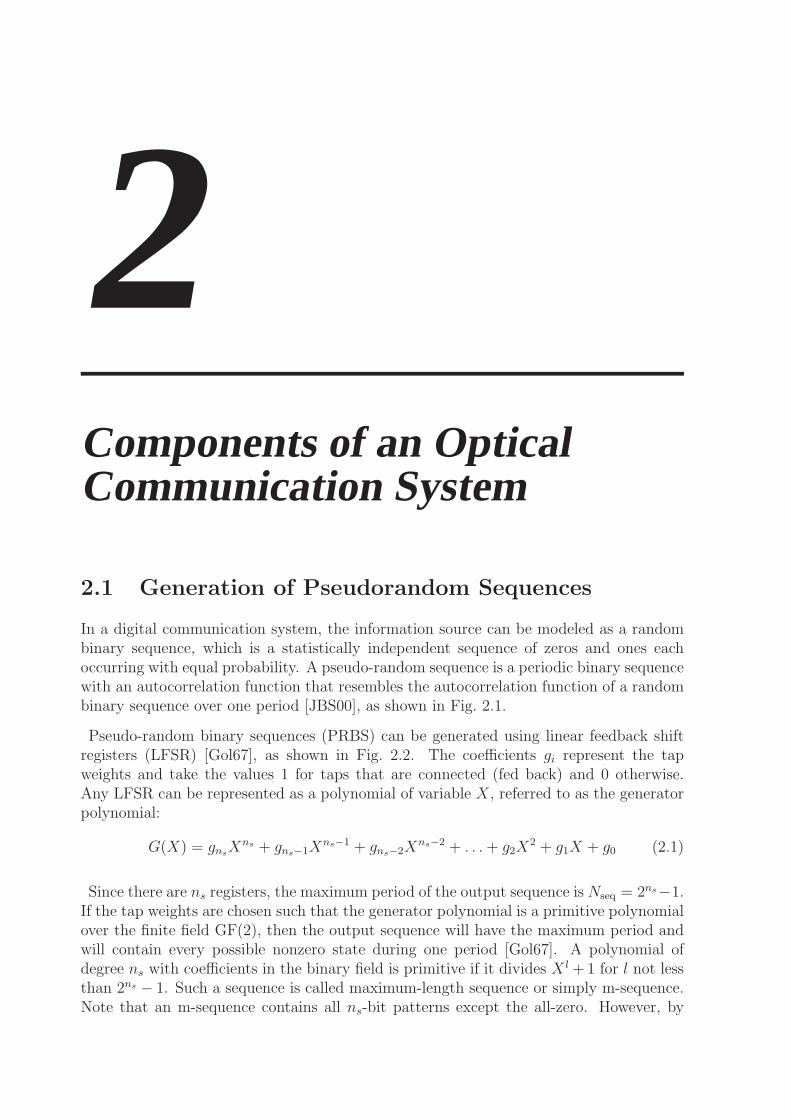
In a digital communication system, the information source can be modeled as a randombinary sequence, which is a statistically independent sequence of zeros and ones eachoccurring with equal probability. A pseudo-random sequence is a periodic binary sequencewith an autocorrelation function that resembles the autocorrelation function of a randombinary sequence over one period [JBS00], as shown in Fig. 2.1.
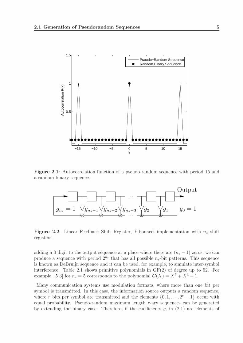
Pseudo-random binary sequences (PRBS) can be generated using linear feedback shiftregisters (LFSR) [Gol67], as shown in Fig. 2.2. The coefficients gi represent the tapweights and take the values 1 for taps that are connected (fed back) and 0 otherwise.Any LFSR can be represented as a polynomial of variable X, referred to as the generatorpolynomial:
G(X) = gnsXns + gns−1X
ns−1 + gns−2Xns−2 + . . . + g2X
2 + g1X + g0 (2.1)
Since there are ns registers, the maximum period of the output sequence is Nseq = 2ns−1.If the tap weights are chosen such that the generator polynomial is a primitive polynomialover the finite field GF(2), then the output sequence will have the maximum period andwill contain every possible nonzero state during one period [Gol67]. A polynomial ofdegree ns with coefficients in the binary field is primitive if it divides X l + 1 for l not lessthan 2ns − 1. Such a sequence is called maximum-length sequence or simply m-sequence.Note that an m-sequence contains all ns-bit patterns except the all-zero. However, by
2.1 Generation of Pseudorandom Sequences 5
−15 −10 −5 0 5 10 15
0
0.5
1
1.5
k
Aut
ocor
rela
tion
R(k
)Pseudo−Random SequenceRandom Binary Sequence
Figure 2.1: Autocorrelation function of a pseudo-random sequence with period 15 anda random binary sequence.
gns−1 g2 g0 = 1
Output
g1gns−2 gns−3gns= 1
Figure 2.2: Linear Feedback Shift Register, Fibonacci implementation with ns shiftregisters.
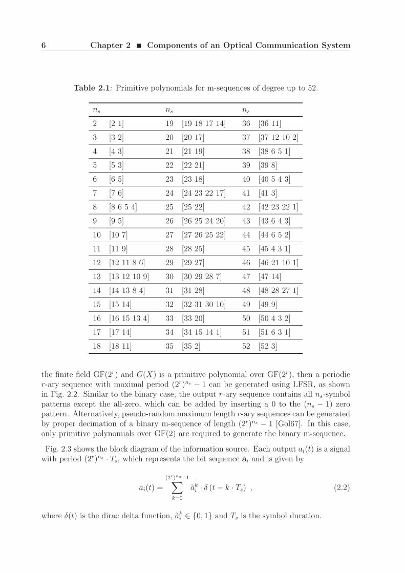
adding a 0 digit to the output sequence at a place where there are (ns − 1) zeros, we canproduce a sequence with period 2ns that has all possible ns-bit patterns. This sequenceis known as DeBruijn sequence and it can be used, for example, to simulate inter-symbolinterference. Table 2.1 shows primitive polynomials in GF(2) of degree up to 52. Forexample, [5 3] for ns = 5 corresponds to the polynomial G(X) = X5 + X3 + 1.
Many communication systems use modulation formats, where more than one bit persymbol is transmitted. In this case, the information source outputs a random sequence,where r bits per symbol are transmitted and the elements 0, 1, . . . , 2r − 1 occur withequal probability. Pseudo-random maximum length r-ary sequences can be generatedby extending the binary case. Therefore, if the coefficients gi in (2.1) are elements of
6 Chapter 2 ¥ Components of an Optical Communication System
Table 2.1: Primitive polynomials for m-sequences of degree up to 52.
ns ns ns
2 [2 1] 19 [19 18 17 14] 36 [36 11]
3 [3 2] 20 [20 17] 37 [37 12 10 2]
4 [4 3] 21 [21 19] 38 [38 6 5 1]
5 [5 3] 22 [22 21] 39 [39 8]
6 [6 5] 23 [23 18] 40 [40 5 4 3]
7 [7 6] 24 [24 23 22 17] 41 [41 3]
8 [8 6 5 4] 25 [25 22] 42 [42 23 22 1]
9 [9 5] 26 [26 25 24 20] 43 [43 6 4 3]
10 [10 7] 27 [27 26 25 22] 44 [44 6 5 2]
11 [11 9] 28 [28 25] 45 [45 4 3 1]
12 [12 11 8 6] 29 [29 27] 46 [46 21 10 1]
13 [13 12 10 9] 30 [30 29 28 7] 47 [47 14]
14 [14 13 8 4] 31 [31 28] 48 [48 28 27 1]
15 [15 14] 32 [32 31 30 10] 49 [49 9]
16 [16 15 13 4] 33 [33 20] 50 [50 4 3 2]
17 [17 14] 34 [34 15 14 1] 51 [51 6 3 1]
18 [18 11] 35 [35 2] 52 [52 3]
the finite field GF(2r) and G(X) is a primitive polynomial over GF(2r), then a periodicr-ary sequence with maximal period (2r)ns − 1 can be generated using LFSR, as shownin Fig. 2.2. Similar to the binary case, the output r-ary sequence contains all ns-symbolpatterns except the all-zero, which can be added by inserting a 0 to the (ns − 1) zeropattern. Alternatively, pseudo-random maximum length r-ary sequences can be generatedby proper decimation of a binary m-sequence of length (2r)ns − 1 [Gol67]. In this case,only primitive polynomials over GF(2) are required to generate the binary m-sequence.
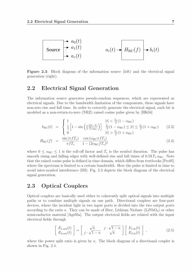
Fig. 2.3 shows the block diagram of the information source. Each output ai(t) is a signalwith period (2r)ns · Ts, which represents the bit sequence ai and is given by
ai(t) =
(2r)ns−1∑
k=0
aki · δ (t − k · Ts) , (2.2)
where δ(t) is the dirac delta function, aki ∈ 0, 1 and Ts is the symbol duration.
2.2 Electrical Signal Generation 7
Source HRC(f) bi(t)ai(t)a1(t)
ar(t)
a0(t)
Figure 2.3: Block diagram of the information source (left) and the electrical signalgeneration (right).
2.2 Electrical Signal Generation
The information source generates pseudo-random sequences, which are represented aselectrical signals. Due to the bandwidth limitation of the components, these signals havenon-zero rise and fall time. In order to correctly generate the electrical signal, each bit ismodeled as a non-return-to-zero (NRZ) raised cosine pulse given by [HK04]
hRC(t) =
1 |t| < Ts
2(1 − αRC)
12
[1 − sin
(π2
2|t|−Ts
TsαRC
)]Ts
2(1 − αRC) ≤ |t| ≤ Ts
2(1 + αRC)
0 |t| > Ts
2(1 + αRC)
(2.3)
HRC(f) =sin (πfTs)
πfTs
· cos (αRCπfTs)
1 − (2αRCfTs)2(2.4)
where 0 ≤ αRC ≤ 1 is the roll-off factor and Ts is the symbol duration. The pulse hassmooth rising and falling edges with well-defined rise and fall times of 0.59 Ts αRC. Notethat the raised cosine pulse is defined in time domain, which differs from textbooks [Pro95]where the spectrum is limited to a certain bandwidth. Here the pulse is limited in time toavoid inter-symbol interference (ISI). Fig. 2.3 depicts the block diagram of the electricalsignal generation.
2.3 Optical Couplers
Optical couplers are basically used either to coherently split optical signals into multiplepaths or to combine multiple signals on one path. Directional couplers are four-portdevices, where the incident light in two input ports is divided into the two output portsaccording to the ratio κ. They can be made of fiber, Lithium Niobate (LiNbO3) or othersemiconductor material [Agr05a]. The output electrical fields are related with the inputelectrical fields through
[E1,out(t)E2,out(t)
]=
[ √κ j ·
√1 − κ
j ·√
1 − κ√
κ
] [E1,in(t)E2,in(t)
], (2.5)
where the power split ratio is given by κ. The block diagram of a directional coupler isshown in Fig. 2.4.
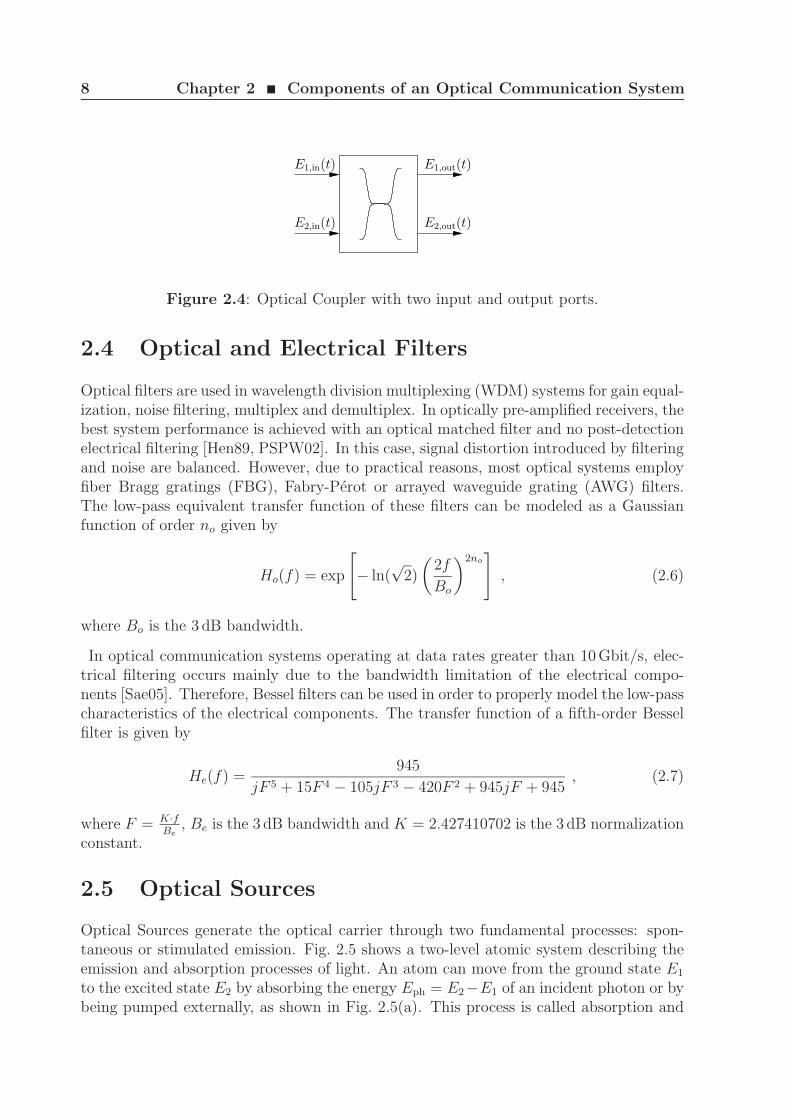
8 Chapter 2 ¥ Components of an Optical Communication System
E1,in(t)
E2,in(t)
E1,out(t)
E2,out(t)
Figure 2.4: Optical Coupler with two input and output ports.
2.4 Optical and Electrical Filters
Optical filters are used in wavelength division multiplexing (WDM) systems for gain equal-ization, noise filtering, multiplex and demultiplex. In optically pre-amplified receivers, thebest system performance is achieved with an optical matched filter and no post-detectionelectrical filtering [Hen89, PSPW02]. In this case, signal distortion introduced by filteringand noise are balanced. However, due to practical reasons, most optical systems employfiber Bragg gratings (FBG), Fabry-Perot or arrayed waveguide grating (AWG) filters.The low-pass equivalent transfer function of these filters can be modeled as a Gaussianfunction of order no given by
Ho(f) = exp
[− ln(
√2)
(2f
Bo
)2no
], (2.6)
where Bo is the 3 dB bandwidth.
In optical communication systems operating at data rates greater than 10 Gbit/s, elec-trical filtering occurs mainly due to the bandwidth limitation of the electrical compo-nents [Sae05]. Therefore, Bessel filters can be used in order to properly model the low-passcharacteristics of the electrical components. The transfer function of a fifth-order Besselfilter is given by
He(f) =945
jF 5 + 15F 4 − 105jF 3 − 420F 2 + 945jF + 945, (2.7)
where F = K·fBe
, Be is the 3 dB bandwidth and K = 2.427410702 is the 3 dB normalizationconstant.
2.5 Optical Sources
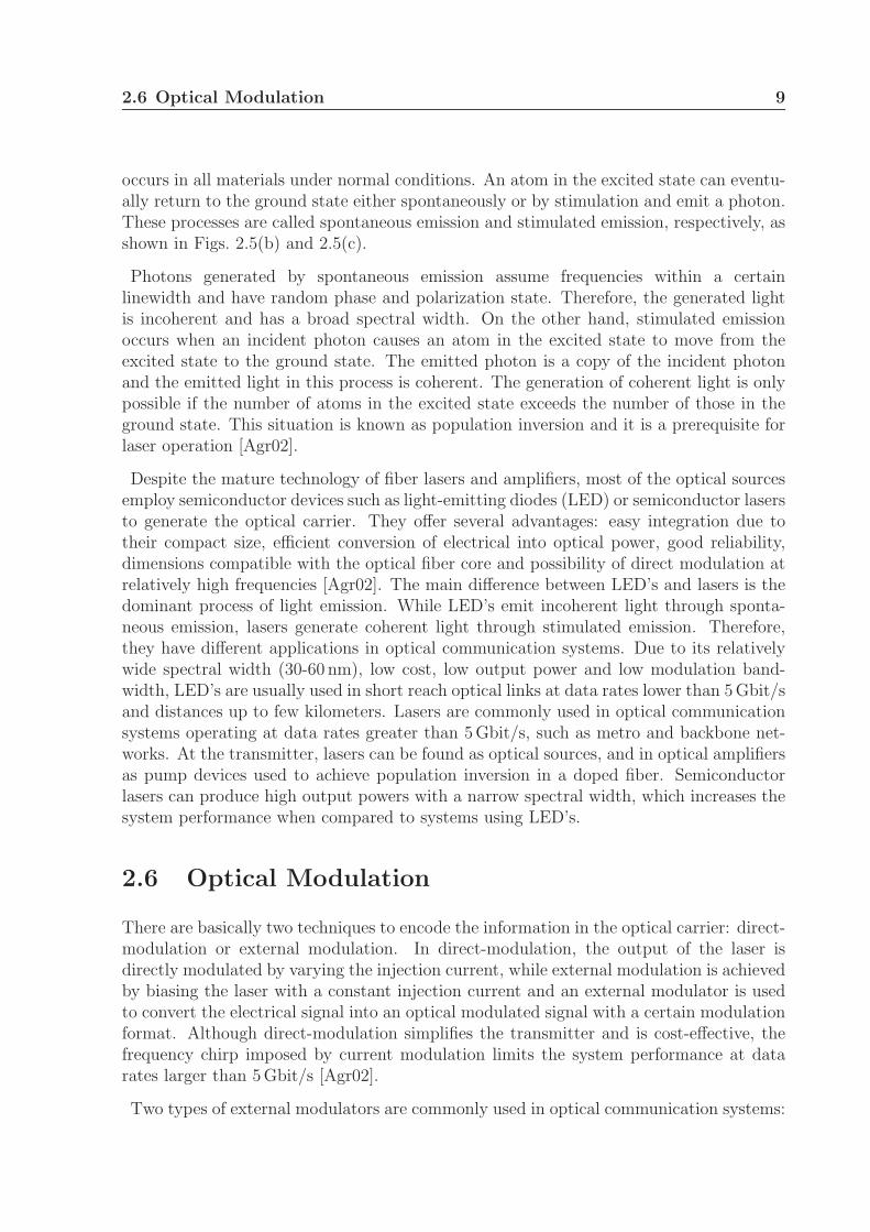
Optical Sources generate the optical carrier through two fundamental processes: spon-taneous or stimulated emission. Fig. 2.5 shows a two-level atomic system describing theemission and absorption processes of light. An atom can move from the ground state E1
to the excited state E2 by absorbing the energy Eph = E2−E1 of an incident photon or bybeing pumped externally, as shown in Fig. 2.5(a). This process is called absorption and
2.6 Optical Modulation 9
occurs in all materials under normal conditions. An atom in the excited state can eventu-ally return to the ground state either spontaneously or by stimulation and emit a photon.These processes are called spontaneous emission and stimulated emission, respectively, asshown in Figs. 2.5(b) and 2.5(c).
Photons generated by spontaneous emission assume frequencies within a certainlinewidth and have random phase and polarization state. Therefore, the generated lightis incoherent and has a broad spectral width. On the other hand, stimulated emissionoccurs when an incident photon causes an atom in the excited state to move from theexcited state to the ground state. The emitted photon is a copy of the incident photonand the emitted light in this process is coherent. The generation of coherent light is onlypossible if the number of atoms in the excited state exceeds the number of those in theground state. This situation is known as population inversion and it is a prerequisite forlaser operation [Agr02].
Despite the mature technology of fiber lasers and amplifiers, most of the optical sourcesemploy semiconductor devices such as light-emitting diodes (LED) or semiconductor lasersto generate the optical carrier. They offer several advantages: easy integration due totheir compact size, efficient conversion of electrical into optical power, good reliability,dimensions compatible with the optical fiber core and possibility of direct modulation atrelatively high frequencies [Agr02]. The main difference between LED’s and lasers is thedominant process of light emission. While LED’s emit incoherent light through sponta-neous emission, lasers generate coherent light through stimulated emission. Therefore,they have different applications in optical communication systems. Due to its relativelywide spectral width (30-60 nm), low cost, low output power and low modulation band-width, LED’s are usually used in short reach optical links at data rates lower than 5 Gbit/sand distances up to few kilometers. Lasers are commonly used in optical communicationsystems operating at data rates greater than 5 Gbit/s, such as metro and backbone net-works. At the transmitter, lasers can be found as optical sources, and in optical amplifiersas pump devices used to achieve population inversion in a doped fiber. Semiconductorlasers can produce high output powers with a narrow spectral width, which increases thesystem performance when compared to systems using LED’s.
2.6 Optical Modulation
There are basically two techniques to encode the information in the optical carrier: direct-modulation or external modulation. In direct-modulation, the output of the laser isdirectly modulated by varying the injection current, while external modulation is achievedby biasing the laser with a constant injection current and an external modulator is usedto convert the electrical signal into an optical modulated signal with a certain modulationformat. Although direct-modulation simplifies the transmitter and is cost-effective, thefrequency chirp imposed by current modulation limits the system performance at datarates larger than 5 Gbit/s [Agr02].
Two types of external modulators are commonly used in optical communication systems:
10 Chapter 2 ¥ Components of an Optical Communication System
Pump
Ground State E1
Excited State E2
PhotonExternal
(a)
Excited State E2
Photon
Ground State E1
(b)
Excited State E2
Photon
Ground State E1
(c)
Figure 2.5: Two-level atomic system describing the three fundamental processes: (a) ab-sorption, (b) spontaneous emission and (c) stimulated emission.
the electro-absorption modulator (EAM) and the Mach-Zehnder modulator (MZM). Inan EAM, the light is modulated by applying a voltage across a semiconductor materialand, therefore, changing its absorption coefficient. In an integrated MZM, the principleof the Mach-Zehnder interferometer and the linear electro-optic effect in Lithium Niobate(LiNbO3) materials [Agr05a] are used for modulation.
The design of an external modulator should consider several parameters such as mod-ulation bandwidth, applied voltage, insertion loss, frequency chirp and extinction ratio.The insertion loss of an EAM can be considerably reduced by integrating the EAM anda continuous wave (CW) laser source on the same chip. This device is known as electro-absorption modulated laser (EML) and can be applied to optical communication systemswhere optical power, extinction ratio and frequency chirp are not critical issues [LY03], forexample, access networks. Compared to EAM, LiNbO3-MZM’s have high extinction ratio,broad optical bandwidth, zero or tunable frequency chirp and temperature insensitivity.The main disadvantages of MZM’s include sensitivity to the polarization of the opticalsignal, bias-drifting, its large size and, consequently, high insertion loss and difficultyto be integrated with other components [LY03]. However, its superior frequency chirpand extinction ratio characteristics make the MZM the first choice for several long-haulfiber-optic communication links. Moreover, MZM can handle high powers and advancedmodulation formats can be easily implemented by combining MZM’s and phase modu-lators. Following, the structures of a LiNbO3 MZM and a LiNbO3 phase modulator arediscussed.
2.6.1 Mach-Zehnder modulator
The Mach-Zehnder modulator uses a titanium-diffused Lithium Niobate (Ti : LiNbO3)waveguide and the principle of the Mach-Zehnder interferometer to modulate the propa-gating light. The presence of Ti atoms within the LiNbO3 crystal increases the refractiveindex by ∼ 0.01 and thus forms a waveguide. The best modulation efficiency is achieved
2.6 Optical Modulation 11
Source
LASER
HRC(f)a0(t) b0(t)
Ein(t) Eout(t)
(a)
LiNbO3 substrate
Eout(t)
v(t)
y
z
x
Ein(t)
Ti:LiNbO3
Waveguide
(b)
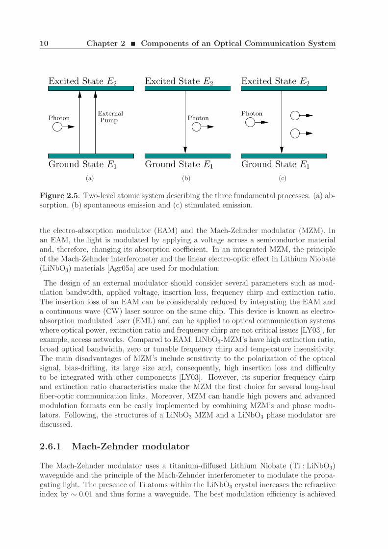
Figure 2.6: Block diagram of a transmitter employing one MZM (a) and X-cut LiNbO3
modulator in the Mach-Zehnder configuration (b).
when the electric fields of the data signal and optical carrier are along the z-axis of thecrystal. Therefore, there are two possible crystal cuts that affects the modulator perfor-mance: X-cut and Z-cut. In both cases the modulation bandwidth and driving voltageare in a tradeoff relationship and the performance is similar [Nog07]. An important pa-rameter in the design of a MZM is the required driving voltage Vπ to produce a phase shiftof π between the two arms of the MZM. The driving voltage Vπ is typically 5 V, but itcan be reduced down to 3 V with a proper design [WKYY+00]. Moreover, the extinctionratio of LiNbO3 modulators can be greater than 20 dB and the modulation bandwidthup to 100 GHz [Nog07]. Figs. 2.6(a) and 2.6(b) show the block diagram of a transmitteremploying only one MZM and the waveguide model for a X-cut MZM.
In Fig. 2.6(b), the electric field of the light can be modulated by using the fact thatthe refractive index of the material LiNbO3 can be changed by applying an external volt-age (electro-optic effect). If no voltage is applied, the optical fields in the two arms of theMach-Zehnder interferometer experience identical phase shift and interfere constructively.If an external voltage is applied, the phase shift in the two arms is no longer identical.Therefore, the intensity of the light is reduced proportionally to the phase difference be-
12 Chapter 2 ¥ Components of an Optical Communication System
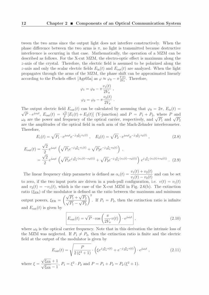
tween the two arms since the output light does not interfere constructively. When thephase difference between the two arms is π, no light is transmitted because destructiveinterference is occurring in that case. Mathematically, the operation of a MZM can bedescribed as follows. For the X-cut MZM, the electro-optic effect is maximum along thez-axis of the crystal. Therefore, the electric field is assumed to be polarized along thez-axis and only the scalar electric fields Ein(t) and Eout(t) are analyzed. When the lightpropagates through the arms of the MZM, the phase shift can be approximated linearlyaccording to the Pockels effect [Agr05a] as ϕ ≈ ϕ0 − π V (t)
2Vπ. Therefore,
ϕ1 = ϕ0 − πv1(t)
2Vπ
,
ϕ2 = ϕ0 − πv2(t)
2Vπ
.
The output electric field Eout(t) can be calculated by assuming that ϕ0 = 2π, Ein(t) =√P · ejω0t, Eout(t) =
√2
2[E1(t) + E2(t)] (Y-junction) and P = P1 + P2, where P and
ω0 are the power and frequency of the optical carrier, respectively, and√
P1 and√
P2
are the amplitudes of the optical field in each arm of the Mach-Zehnder interferometer.Therefore,
E1(t) =√
P1 · ejω0te−j π2Vπ
v1(t) , E2(t) =√
P2 · ejω0te−j π2Vπ
v2(t) , (2.8)
Eout(t) =
√2
2ejω0t
(√P1e
−j π2Vπ
v1(t) +√
P2e−j π
2Vπv2(t)
),
=
√2
2ejω0t
(√P1e
j π4Vπ
(v1(t)−v2(t)) +√
P2e−j π
4Vπ(v1(t)−v2(t))
)ej π
4Vπ(v1(t)+v2(t)) . (2.9)
The linear frequency chirp parameter is defined as αc(t) =v1(t) + v2(t)
v1(t) − v2(t)and can be set
to zero, if the two input ports are driven in a push-pull configuration, i.e. v(t) = v1(t)and v2(t) = −v1(t), which is the case of the X-cut MZM in Fig. 2.6(b). The extinctionratio (ξER) of the modulator is defined as the ratio between the maximum and minimum
output powers, ξER =
(√P1 +
√P2√
P1 −√
P2
)2
. If P1 = P2, then the extinction ratio is infinite
and Eout(t) is given by
Eout(t) =√
P · cos
(π
2Vπ
v(t)
)· ejω0t , (2.10)
where ω0 is the optical carrier frequency. Note that in this derivation the intrinsic loss ofthe MZM was neglected. If P1 6= P2, then the extinction ratio is finite and the electricfield at the output of the modulator is given by
Eout(t) =
√P
2 (ξ2 + 1)·(ξej π
2Vπv(t) + e−j π
2Vπv(t)
)· ejω0t , (2.11)
where ξ =
√ξER + 1√ξER − 1
, P1 = ξ2 · P2 and P = P1 + P2 = P2 (ξ2 + 1).
2.7 Optical Amplification 13
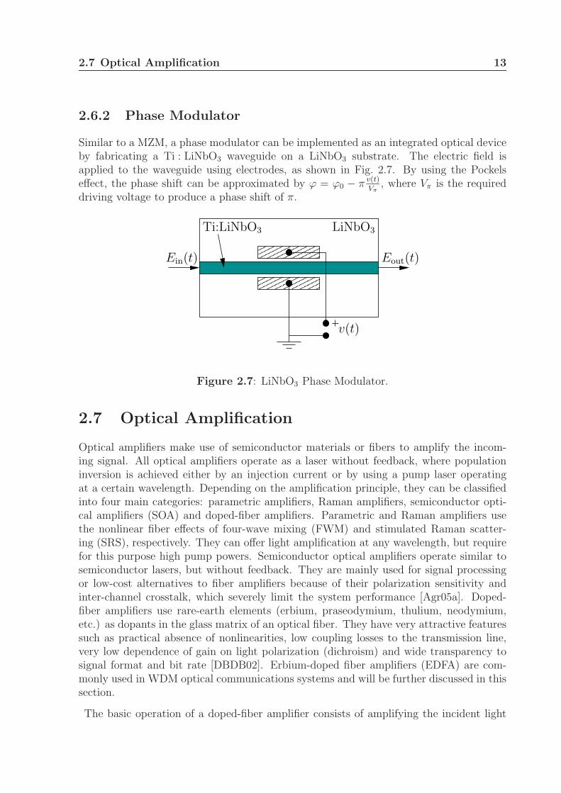
2.6.2 Phase Modulator
Similar to a MZM, a phase modulator can be implemented as an integrated optical deviceby fabricating a Ti : LiNbO3 waveguide on a LiNbO3 substrate. The electric field isapplied to the waveguide using electrodes, as shown in Fig. 2.7. By using the Pockelseffect, the phase shift can be approximated by ϕ = ϕ0 − π v(t)
Vπ, where Vπ is the required
driving voltage to produce a phase shift of π.
v(t)
Ein(t) Eout(t)
Ti:LiNbO3 LiNbO3
Figure 2.7: LiNbO3 Phase Modulator.
2.7 Optical Amplification
Optical amplifiers make use of semiconductor materials or fibers to amplify the incom-ing signal. All optical amplifiers operate as a laser without feedback, where populationinversion is achieved either by an injection current or by using a pump laser operatingat a certain wavelength. Depending on the amplification principle, they can be classifiedinto four main categories: parametric amplifiers, Raman amplifiers, semiconductor opti-cal amplifiers (SOA) and doped-fiber amplifiers. Parametric and Raman amplifiers usethe nonlinear fiber effects of four-wave mixing (FWM) and stimulated Raman scatter-ing (SRS), respectively. They can offer light amplification at any wavelength, but requirefor this purpose high pump powers. Semiconductor optical amplifiers operate similar tosemiconductor lasers, but without feedback. They are mainly used for signal processingor low-cost alternatives to fiber amplifiers because of their polarization sensitivity andinter-channel crosstalk, which severely limit the system performance [Agr05a]. Doped-fiber amplifiers use rare-earth elements (erbium, praseodymium, thulium, neodymium,etc.) as dopants in the glass matrix of an optical fiber. They have very attractive featuressuch as practical absence of nonlinearities, low coupling losses to the transmission line,very low dependence of gain on light polarization (dichroism) and wide transparency tosignal format and bit rate [DBDB02]. Erbium-doped fiber amplifiers (EDFA) are com-monly used in WDM optical communications systems and will be further discussed in thissection.
The basic operation of a doped-fiber amplifier consists of amplifying the incident light
14 Chapter 2 ¥ Components of an Optical Communication System
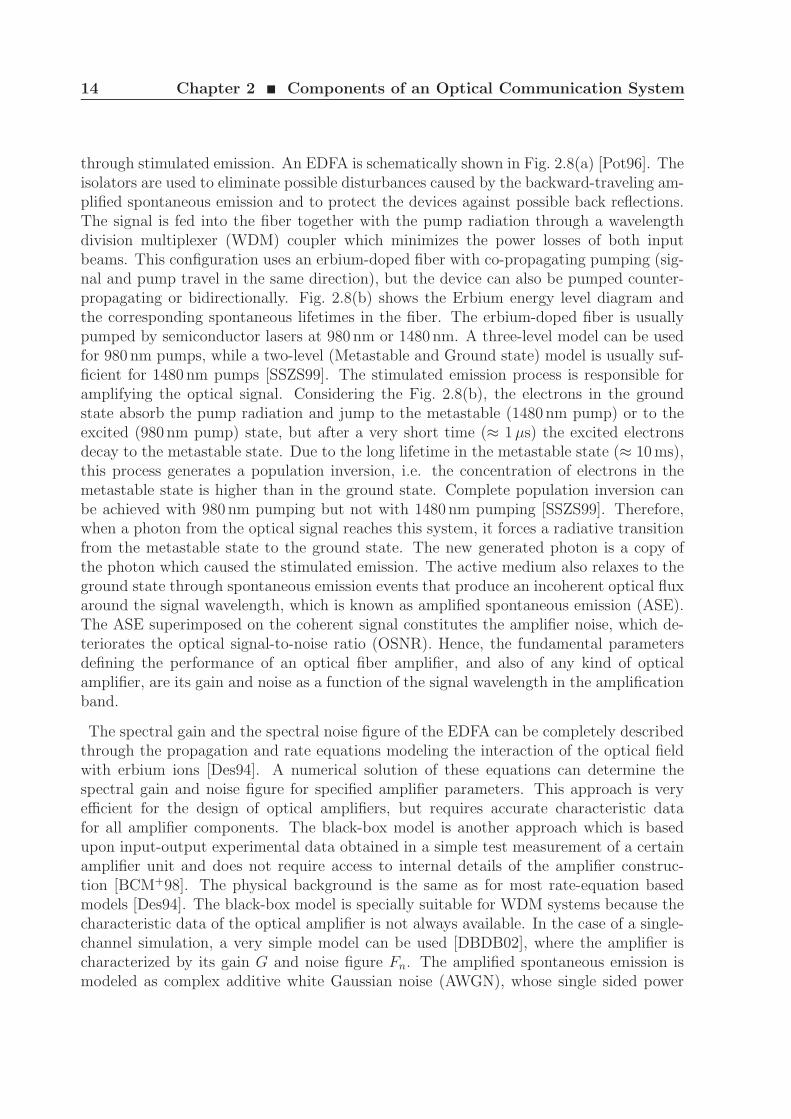
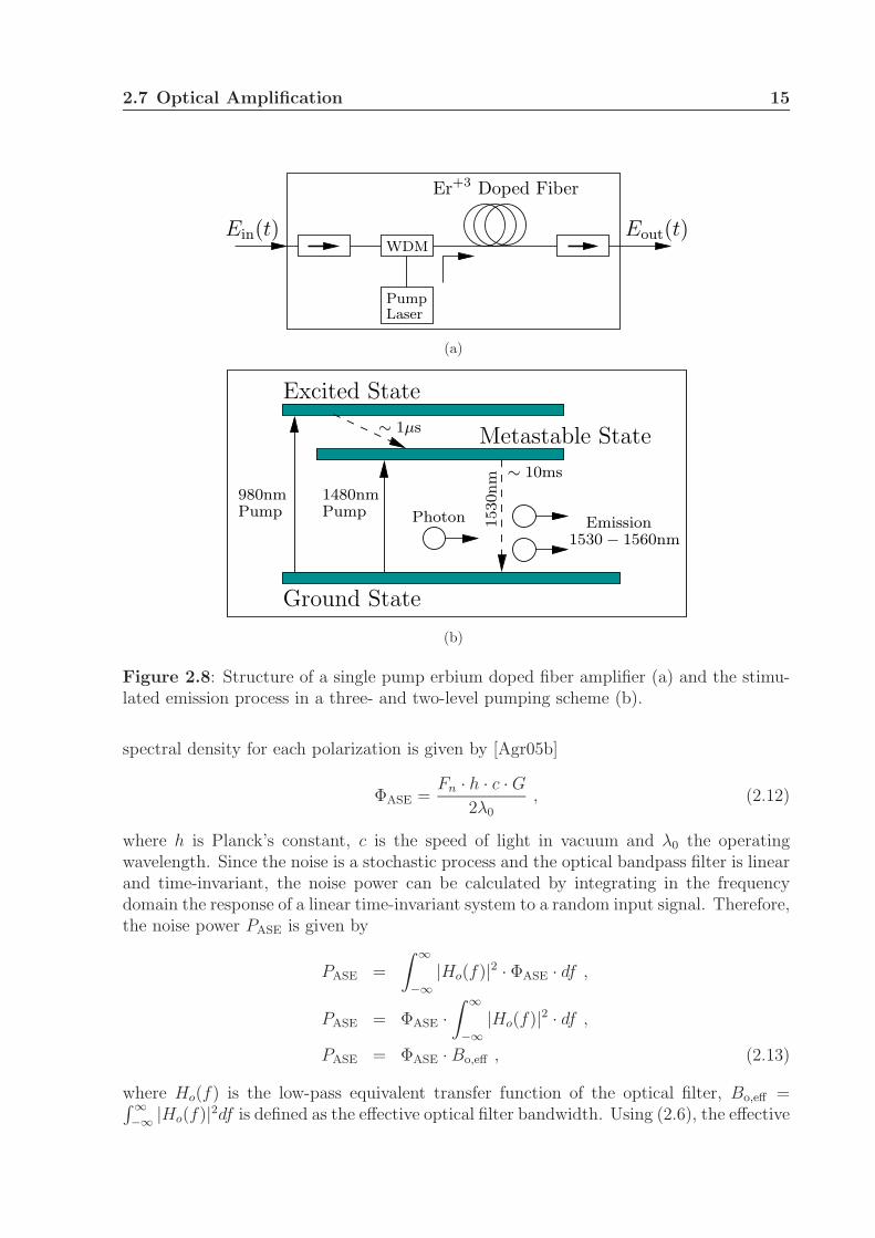
through stimulated emission. An EDFA is schematically shown in Fig. 2.8(a) [Pot96]. Theisolators are used to eliminate possible disturbances caused by the backward-traveling am-plified spontaneous emission and to protect the devices against possible back reflections.The signal is fed into the fiber together with the pump radiation through a wavelengthdivision multiplexer (WDM) coupler which minimizes the power losses of both inputbeams. This configuration uses an erbium-doped fiber with co-propagating pumping (sig-nal and pump travel in the same direction), but the device can also be pumped counter-propagating or bidirectionally. Fig. 2.8(b) shows the Erbium energy level diagram andthe corresponding spontaneous lifetimes in the fiber. The erbium-doped fiber is usuallypumped by semiconductor lasers at 980 nm or 1480 nm. A three-level model can be usedfor 980 nm pumps, while a two-level (Metastable and Ground state) model is usually suf-ficient for 1480 nm pumps [SSZS99]. The stimulated emission process is responsible foramplifying the optical signal. Considering the Fig. 2.8(b), the electrons in the groundstate absorb the pump radiation and jump to the metastable (1480 nm pump) or to theexcited (980 nm pump) state, but after a very short time (≈ 1 µs) the excited electronsdecay to the metastable state. Due to the long lifetime in the metastable state (≈ 10 ms),this process generates a population inversion, i.e. the concentration of electrons in themetastable state is higher than in the ground state. Complete population inversion canbe achieved with 980 nm pumping but not with 1480 nm pumping [SSZS99]. Therefore,when a photon from the optical signal reaches this system, it forces a radiative transitionfrom the metastable state to the ground state. The new generated photon is a copy ofthe photon which caused the stimulated emission. The active medium also relaxes to theground state through spontaneous emission events that produce an incoherent optical fluxaround the signal wavelength, which is known as amplified spontaneous emission (ASE).The ASE superimposed on the coherent signal constitutes the amplifier noise, which de-teriorates the optical signal-to-noise ratio (OSNR). Hence, the fundamental parametersdefining the performance of an optical fiber amplifier, and also of any kind of opticalamplifier, are its gain and noise as a function of the signal wavelength in the amplificationband.
The spectral gain and the spectral noise figure of the EDFA can be completely describedthrough the propagation and rate equations modeling the interaction of the optical fieldwith erbium ions [Des94]. A numerical solution of these equations can determine thespectral gain and noise figure for specified amplifier parameters. This approach is veryefficient for the design of optical amplifiers, but requires accurate characteristic datafor all amplifier components. The black-box model is another approach which is basedupon input-output experimental data obtained in a simple test measurement of a certainamplifier unit and does not require access to internal details of the amplifier construc-tion [BCM+98]. The physical background is the same as for most rate-equation basedmodels [Des94]. The black-box model is specially suitable for WDM systems because thecharacteristic data of the optical amplifier is not always available. In the case of a single-channel simulation, a very simple model can be used [DBDB02], where the amplifier ischaracterized by its gain G and noise figure Fn. The amplified spontaneous emission ismodeled as complex additive white Gaussian noise (AWGN), whose single sided power
2.7 Optical Amplification 15
Pump
Ein(t) Eout(t)
Er+3 Doped Fiber
WDM
Laser
(a)
Emission
∼ 1µs
Ground State
1530nm
Excited State
Metastable State
980nmPump Photon
∼ 10ms
1480nmPump
1530 − 1560nm
(b)
Figure 2.8: Structure of a single pump erbium doped fiber amplifier (a) and the stimu-lated emission process in a three- and two-level pumping scheme (b).
spectral density for each polarization is given by [Agr05b]
ΦASE =Fn · h · c · G
2λ0
, (2.12)
where h is Planck’s constant, c is the speed of light in vacuum and λ0 the operatingwavelength. Since the noise is a stochastic process and the optical bandpass filter is linearand time-invariant, the noise power can be calculated by integrating in the frequencydomain the response of a linear time-invariant system to a random input signal. Therefore,the noise power PASE is given by
PASE =
∫ ∞
−∞|Ho(f)|2 · ΦASE · df ,
PASE = ΦASE ·∫ ∞
−∞|Ho(f)|2 · df ,
PASE = ΦASE · Bo,eff , (2.13)
where Ho(f) is the low-pass equivalent transfer function of the optical filter, Bo,eff =∫ ∞−∞ |Ho(f)|2df is defined as the effective optical filter bandwidth. Using (2.6), the effective
16 Chapter 2 ¥ Components of an Optical Communication System
optical filter bandwidth is given by
Bo,eff =BoΓ
(1
2no
)
2no (ln(2))1
2no
, (2.14)
where Γ(·) is the Gamma function, Bo the 3 dB bandwidth and no the order of theGaussian optical filter.
2.8 Photodetection
The main task of a photodetector is to convert the optical signal into an electrical signalthrough the photoelectric effect. The main requirements for a photodetector are: highsensitivity, high response bandwidth, low noise, low cost and high reliability [Agr05a].In this thesis, the photodetector consists of an ideal p-i-n photodiode with responsivityR =1 A/W. In Fig. 2.9, the output in time and frequency domains is given by
Iout(t) = |Ein(t)|2 , (2.15)
Iout(f) = Ein(f) ∗ E∗in(−f) , (2.16)
where the operator ∗ denotes the convolutional operation.
Iout(t)Ein(t)
Figure 2.9: Ideal photodiode.
2.9 Propagation of Light in Optical Fibers
The starting point of the analysis of light propagation in optical fibers are the Maxwell’sequations:
∇× E = −∂B
∂t(2.17)
∇× H =∂D
∂t(2.18)
∇ · D = 0 (2.19)
∇ · B = 0 (2.20)
The electric and magnetic field vectors, E and H, respectively, are related to theircorresponding flux densities, D and B, by the constitutive relations
D = ǫ0E + P , (2.21)
B = µ0H + M , (2.22)
2.9 Propagation of Light in Optical Fibers 17
where ǫ0 is the vacuum permittivity, µ0 is the vacuum permeability, and P and M arethe induced electric and magnetic polarizations, respectively. For a nonmagnetic mediumsuch as optical fibers, M = 0. By taking the curl of (2.17) and using (2.18), (2.21), (2.22),we obtain
∇×∇× E = −∇× ∂B
∂t
= −µ0∇× H
∂t
= −µ0∂2D
∂t2
= −µ0ǫ0∂2E
∂t2− µ0∂
2P
∂t2. (2.23)
Using the identity ∇×∇× E = ∇(∇ · E) −∇2E, (2.23) can be written as
∇(∇ · E) −∇2E = −µ0ǫ0∂2E
∂t2− µ0∂
2P
∂t2(2.24)
∇2E −∇(∇ · E) − 1
c2
∂2E
∂t2= µ0
∂2P
∂t2, (2.25)
where c = (µ0ǫ0)− 1
2 is the speed of light in vacuum. The optical fiber is also a nonlinearmedium and is characterized by a nonlinear relation between P and E. Therefore, it isconvenient to separate P into its linear PL and nonlinear PNL parts. Using (2.19) andassuming that the nonlinear response of the optical fiber is small, the induced electricpolarization can be written as P = ǫE, which results in ∇(∇ · E) ≈ 0 and
∇2E − 1
c2
∂2E
∂t2= µ0
∂2PL
∂t2+ µ0
∂2PNL
∂t2. (2.26)
The function that relates P(r, t) and E(r, t) can also be expanded in a power seriesas [Sch04, Agr06]
P(r, t) = P(1)L (r, t) + P
(2)NL(r, t) + P
(3)NL(r, t) + . . . (2.27)
= ǫ0
∫ t
−∞χ(1)(t − t′) · E(r, t′)dt′
+ ǫ0
t∫∫
−∞
dt1 dt2 χ(2)(t − t1, t − t2) : E(r, t1)E(r, t2)
+ ǫ0
t∫∫∫
−∞
dt1 dt2 dt3 χ(3)(t − t1, t − t2, t − t3)...E(r, t1)E(r, t2)E(r, t3) + . . . ,
(2.28)
18 Chapter 2 ¥ Components of an Optical Communication System
where r is the spatial coordinate and χ(i) is the i-th order susceptibility. The linearsusceptibility χ(1) represents the dominant contribution to P(r, t). Due to the symmetryof the fiber glass, χ(2) is zero. Among all nonlinear terms in (2.27), the third-ordernonlinear susceptibility χ(3) represents the dominant nonlinear contribution to P(r, t)and, therefore, terms higher than three will be neglected. The i-th order susceptibilityχ(i) is a tensor of rank i + 1 with 3i+1 elements. Consequently, the linear part of theinduced electric polarization can be written in a matrix form and in frequency domain as
PL(r, ω) = ǫ0χ(1)(ω) · E(r, ω) (2.29)
P xL (r, ω)
P yL(r, ω)
P zL(r, ω)
= ǫ0
χ(1)xx (ω) χ
(1)xy (ω) χ
(1)xz (ω)
χ(1)yx (ω) χ
(1)yy (ω) χ
(1)yz (ω)
χ(1)zx (ω) χ
(1)zy (ω) χ
(1)zz (ω)
·
Ex(r, ω)
Ey(r, ω)
Ez(r, ω)
(2.30)
Note that each line of the vector PL(r, ω) can be expressed in a summation form as
P iL(r, ω) = ǫ0
∑
j
χ(1)ij (ω) Ej(r, ω) , (2.31)
where i, j ∈ x, y, z. The ideal optical fiber is also an isotropic medium, i.e. theirphysical and optical properties at each point are independent of the direction along whichthe electric field is applied. Therefore, only three elements of the matrix χ(1) are nonzeroand they are approximately equal χ
(1)xx (ω) = χ
(1)yy (ω) = χ
(1)zz (ω). In this case, (2.29) is given
by
PL(r, ω) = ǫ0χ(1)xx (ω) · E(r, ω) . (2.32)
The electric field E(r, t) associated with an arbitrarily polarized optical wave can bewritten as
E(r, t) =
Re Ex(r, t)Re Ey(r, t)Re Ez(r, t)
=
E ′x
E ′y
E ′z
=
E x(r, t)E y(r, t)E z(r, t)
· ejω0t
2+
E∗x(r, t)
E∗y(r, t)
E∗z(r, t)
· e−jω0t
2, (2.33)
where Ei(r, t) = E i(r, t) ejω0t, i ∈ x, y, z, and E i(r, t) is the complex slowly varying am-plitude of the corresponding electric field oscillating at the carrier frequency ω0. In (2.26),the nonlinear part of the induced polarization PNL(r, t) models all nonlinear effects occur-ring in the fiber. Considerable simplification is achieved if Raman and Brillouin effects areneglected, which makes the nonlinear response of the medium instantaneous. Therefore,
2.9 Propagation of Light in Optical Fibers 19
PNL(r, t) in (2.28) can be written as [Agr06]
PNL(r, t) = ǫ0χ(3) ...E(r, t)E(r, t)E(r, t) (2.34)
P xNL(r, t)
P yNL(r, t)
P zNL(r, t)
= ǫ0
χ(3)xxxx χ
(3)xxxy · · · χ
(3)xzzz
χ(3)yxxx χ
(3)yxxy · · · χ
(3)yzzz
χ(3)zxxx χ
(3)zxxy · · · χ
(3)zzzz
·
E ′x E ′
x E ′x
E ′x E ′
x E ′y
· · ·· · ·· · ·
E ′z E ′
z E ′y
E ′z E ′
z E ′z
. (2.35)
where χ(3) is assumed to be constant at the frequency ω0 and real, which is true for alossless medium. Each line of the vector PNL(r, t) can be expressed in a summation formas
P iNL(r, t) = ǫ0
∑
jkl
χ(3)ijkl E
′j E ′
k E ′l , (2.36)
where i, j, k, l ∈ x, y, z. The third-order nonlinear susceptibility χ(3) is a four-ranktensor with 81 elements, but in optical fibers only three terms are independent, whichmeans that each element of χ(3) can be written as
χ(3)ijkl = χ(3)
xxyyδijδkl + χ(3)xyxyδikδjl + χ(3)
xyyxδilδjk , (2.37)
where δab is the Kronecker delta function with δab = 1 when a = b and δab = 0 otherwise.Therefore, there are 21 nonzero elements, whose indices are [Boy08]:
xxyy = yyzz = zzyy = zzxx = xxzz = yyxx
xyxy = yzyz = zyzy = zxzx = xzxz = yxyx
xyyx = yzzy = zyyz = zxxz = xzzx = yxxy
xxxx = yyyy = zzzz = xxyy + xyxy + xyyx
(2.38)
Due to the electronic origin of the physical mechanisms that contribute to χ(3), χ(3)xxyy,
χ(3)xyxy and χ
(3)xyyx have almost the same magnitude and can be considered equal. Therefore,
substituting (2.37) in (2.36) and using (2.33), P iNL(r, t) can be written as
P iNL(r, t) = ǫ0
∑
k
χ(3)xxyy E ′
i E′k E ′
k + χ(3)xyxy E ′
k E ′i E
′k + χ(3)
xyyx E ′k E ′
k E ′i (2.39)
= ǫ0 · χ(3)xxxx
∑
k
E ′i E
′2k (2.40)
=ǫ0 · χ(3)
xxxx
8
∑
k
E i(r, t) E2k(r, t) ej3ω0t + 2E i(r, t) |E k(r, t)|2 ejω0t +
+ E∗i(r, t) E2
k(r, t) ejω0t + c.c. , (2.41)
20 Chapter 2 ¥ Components of an Optical Communication System
where “c.c.” means complex conjugate. The term oscillating at the third-harmonic fre-quency 3ω0 is not phase-matched and is generally negligible in optical fibers. The longi-tudinal component Ez(r, t) of the electric field is so small that it can be neglected whencompared to the transverse components Ex(r, t) and Ey(r, t). Finally, PNL(r, t) is givenby the following equations:
P iNL(r, t) =
ǫ0
8χ(3)
xxxx
∑
k
E∗i (r, t) E2
k(r, t) + 2Ei(r, t) |Ek(r, t)|2 + c.c. (2.42)
P xNL(r, t) =
3ǫ0
4χ
(3)xxxx
(1
2
[(|Ex|2 +
2
3|Ey|2
)Ex +
1
3(E∗
xEy)Ey
]+ c.c.
)
P yNL(r, t) =
3ǫ0
4χ
(3)xxxx
(1
2
[(|Ey|2 +
2
3|Ex|2
)Ey +
1
3(E∗
yEx)Ex
]+ c.c.
) . (2.43)
Throughout this thesis, the normalized electric field in units of√
W is defined as E(t) =B(t) ·
√Aeff/2ZF , where ZF is the waveguide impedance in Ω, B(z, t) is the amplitude of
the electric field in V/m and Aeff is an effective area, which will be explained later in thissection.
2.9.1 Linear Fibers
The first step in describing the transmission of light through optical fibers consists ofderiving the propagation equation for PNL(r, t) = 0. In this case, (2.26) can be writtenas
∇2E =1
c2·
∂2E
∂t2+
∂2[χ
(1)xx (t) ∗ E(r, t)
]
∂t2
. (2.44)
By taking the Fourier transform, we obtain the Helmholtz equation
∇2E = −ω2
c2E − ω2
c2χ(1)
xx (ω) · E
= −ǫ(r, w) · ω2
c2E
∇2E + ǫ(r, w) k20 E = 0 , (2.45)
where k0 = ω/c is the free-space wave number and ǫ(r, w) = 1 + χ(1)xx (ω) is the frequency-
dependent dielectric constant. The real and imaginary parts of ǫ(r, w) are related to therefractive index n(r, ω) and the absorption or attenuation coefficient α(ω) by using thedefinition
ǫ(r, w) =
(n(r, ω) + j
α(ω) c
2ω
)2
, (2.46)
where
n(r, ω) ≈√
1 + Reχ(1)xx (ω)
α(ω) =ω
n(r, ω) cImχ(1)
xx (ω) .
2.9 Propagation of Light in Optical Fibers 21
The frequency dependence of n(r, ω) is known as material dispersion. In general, ǫ(r, ω)is complex, however, due to low optical losses in silica fibers ǫ(r, ω) can be taken to bereal and replaced by n2(r, ω). Fiber losses will be treated later in this section. Sincefor step-index fibers n(r, ω) is independent of the spatial coordinate r in the core andcladding, (2.45) can be written as
∇2E + n2(ω) k20E = 0 . (2.47)
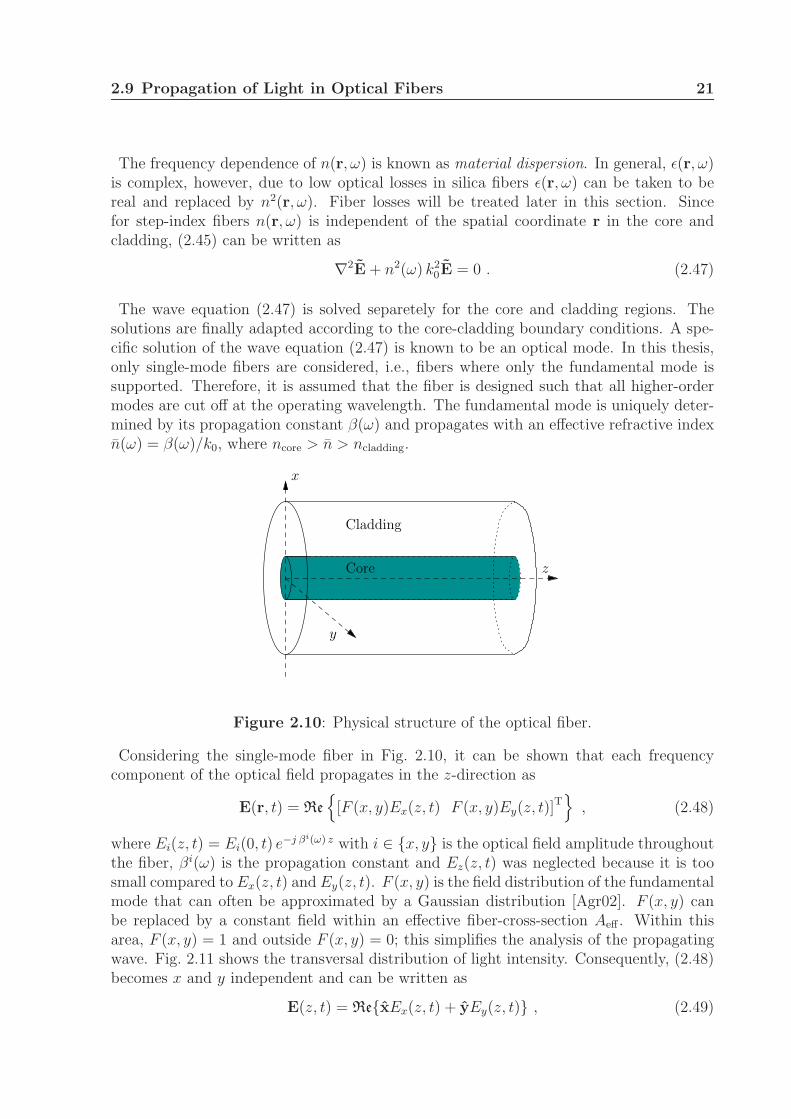
The wave equation (2.47) is solved separetely for the core and cladding regions. Thesolutions are finally adapted according to the core-cladding boundary conditions. A spe-cific solution of the wave equation (2.47) is known to be an optical mode. In this thesis,only single-mode fibers are considered, i.e., fibers where only the fundamental mode issupported. Therefore, it is assumed that the fiber is designed such that all higher-ordermodes are cut off at the operating wavelength. The fundamental mode is uniquely deter-mined by its propagation constant β(ω) and propagates with an effective refractive indexn(ω) = β(ω)/k0, where ncore > n > ncladding.
x
z
y
Cladding
Core
Figure 2.10: Physical structure of the optical fiber.
Considering the single-mode fiber in Fig. 2.10, it can be shown that each frequencycomponent of the optical field propagates in the z-direction as
E(r, t) = Re
[F (x, y)Ex(z, t) F (x, y)Ey(z, t)]
T
, (2.48)
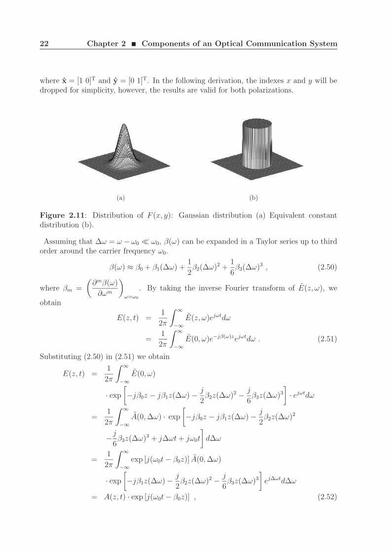
where Ei(z, t) = Ei(0, t) e−j βi(ω) z with i ∈ x, y is the optical field amplitude throughoutthe fiber, βi(ω) is the propagation constant and Ez(z, t) was neglected because it is toosmall compared to Ex(z, t) and Ey(z, t). F (x, y) is the field distribution of the fundamentalmode that can often be approximated by a Gaussian distribution [Agr02]. F (x, y) canbe replaced by a constant field within an effective fiber-cross-section Aeff . Within thisarea, F (x, y) = 1 and outside F (x, y) = 0; this simplifies the analysis of the propagatingwave. Fig. 2.11 shows the transversal distribution of light intensity. Consequently, (2.48)becomes x and y independent and can be written as
E(z, t) = RexEx(z, t) + yEy(z, t) , (2.49)
22 Chapter 2 ¥ Components of an Optical Communication System
where x = [1 0]T and y = [0 1]T. In the following derivation, the indexes x and y will bedropped for simplicity, however, the results are valid for both polarizations.
(a) (b)
Figure 2.11: Distribution of F (x, y): Gaussian distribution (a) Equivalent constantdistribution (b).
Assuming that ∆ω = ω − ω0 ≪ ω0, β(ω) can be expanded in a Taylor series up to thirdorder around the carrier frequency ω0.
β(ω) ≈ β0 + β1(∆ω) +1
2β2(∆ω)2 +
1
6β3(∆ω)3 , (2.50)
where βm =
(∂mβ(ω)
∂ωm
)
ω=ω0
. By taking the inverse Fourier transform of E(z, ω), we
obtain
E(z, t) =1
2π
∫ ∞
−∞E(z, ω)ejωtdω
=1
2π
∫ ∞
−∞E(0, ω)e−jβ(ω)zejωtdω . (2.51)
Substituting (2.50) in (2.51) we obtain
E(z, t) =1
2π
∫ ∞
−∞E(0, ω)
· exp
[−jβ0z − jβ1z(∆ω) − j
2β2z(∆ω)2 − j
6β3z(∆ω)3
]· ejωtdω
=1
2π
∫ ∞
−∞A(0, ∆ω) · exp
[−jβ0z − jβ1z(∆ω) − j
2β2z(∆ω)2
−j
6β3z(∆ω)3 + j∆ωt + jω0t
]d∆ω
=1
2π
∫ ∞
−∞exp [j(ω0t − β0z)] A(0, ∆ω)
· exp
[−jβ1z(∆ω) − j
2β2z(∆ω)2 − j
6β3z(∆ω)3
]ej∆ωtd∆ω
= A(z, t) · exp [j(ω0t − β0z)] , (2.52)
2.9 Propagation of Light in Optical Fibers 23
where ∆ω = ω − ω0, A(0, ∆ω) = E(0, ω) ⇒ E(0, t) = A(0, t) · ejω0t and A(z, t) is theslowly varing amplitude, which is defined as
A(z, t) =1
2π
∫ ∞
−∞A(0, ∆ω) · exp
[−jβ1z(∆ω) − j
2β2z(∆ω)2
−j
6β3z(∆ω)3
]ej∆ωtd∆ω . (2.53)
By calculating∂A(z, ∆ω)
∂zand taking the inverse Fourier transform, (2.53) can be written
in the time domain as
A(z, ∆ω) = A(0, ∆ω) · exp
[−jβ1z(∆ω) − j
2β2z(∆ω)2 − j
6β3z(∆ω)3
]
∂A(z, ∆ω)
∂z= A(z, ∆ω) ·
[−jβ1(∆ω) − j
2β2(∆ω)2 − j
6β3(∆ω)3
]
F−1
∂A(z, ∆ω)
∂z
= F−1
A(z, ∆ω)
·[−jβ1(∆ω) − j
2β2(∆ω)2 − j
6β3(∆ω)3
]
∂A(z, t)
∂z= −β1
∂A(z, t)
∂t+
j
2β2
∂2A(z, t)
∂t2+
1
6β3
∂3A(z, t)
∂t3
∂A(z, t)
∂z+ β1
∂A(z, t)
∂t− j
2β2
∂2A(z, t)
∂t2− 1
6β3
∂3A(z, t)
∂t3= 0 . (2.54)
By performing the transformation t′ = t+β1z and z′ = z, and using the Fourier Transformwe have
∂A(z′, t′ − β1z′)
∂z′+ β1
∂A(z′, t′ − β1z′)
∂t′− j
2β2
∂2A(z′, t′ − β1z′)
∂t′2
− 1
6β3
∂3A(z′, t′ − β1z′)
∂t′3= 0
∂[A(z′, ω)e−jωβ1z′ ]
∂z′+ jβ1ωA(z′, ω)e−jωβ1z′
+j
2β2ω
2A(z′, ω)e−jωβ1z′ +j
6β3ω
3A(z′, ω)e−jωβ1z′ = 0
∂A(z′, ω)
∂z′· e−jωβ1z′ − jβ1ωA(z′, ω)e−jωβ1z′ + jβ1ωA(z′, ω)e−jωβ1z′
+j
2β2ω
2A(z′, ω)e−jωβ1z′ +j
6β3ω
3A(z′, ω)e−jωβ1z′ = 0
∂A(z′, t′)
∂z′− j
2β2
∂2A(z′, t′)
∂t′2− 1
6β3
∂3A(z′, t′)
∂t′3= 0 . (2.55)
24 Chapter 2 ¥ Components of an Optical Communication System
In general, fiber losses are governed by the Beer’s law [Agr02], which can be written interms of A(z, t) as
∂A(z, t)
∂z= −α
2A(z, t) , (2.56)
where α = α(ω0) is assumed to be constant in the vicinity of the carrier frequency ω0.The attenuation is now included in (2.55), which is modeled as
∂A(z, t)
∂z− j
2β2
∂2A(z, t)
∂t2− 1
6β3
∂3A(z, t)
∂t3= −α
2A(z, t) , (2.57)
where β2 is the group-velocity dispersion coefficient in s2/m, β3 is the third-order dispersionparameter in s3/m and α is the attenuation coefficient in (m)−1.
2.9.2 Linear Birefringent Fibers
The single-mode fiber supports two orthogonally polarized modes with the same spatialdistribution, which are represented by the vectors x and y. In absence of birefringence, therefractive indexes of the modes x and y are equal, nx(ω) = ny(ω), while in a birefringentfiber nx(ω) 6= ny(ω). The derivation of (2.57) is valid for a fiber without birefringence,where the polarization state of the incident light is maintained during its propagation. Ifthe fiber is birefringent, then the propagation constant β(ω) assumes different values forthe modes x and y. In absence of fiber nonlinearities, (2.54) can be extended to includebirefringence as follows:
E(z, t) = Re [xEx(z, t) + yEy(z, t)] , see (2.49)
where Ex(z, t) and Ey(z, t) are now given by
Ex(z, t) = Ax(z, t) · exp [j(ω0t − βx0 z)] ,
Ey(z, t) = Ay(z, t) · exp [j(ω0t − βy0z)] ,
and
∂Ax(z, t)
∂z+ βx
1
∂Ax(z, t)
∂t− j
2β2
∂2Ax(z, t)
∂t2− 1
6β3
∂3Ax(z, t)
∂t3= −α
2Ax(z, t)
∂Ay(z, t)
∂z+ βy
1
∂Ay(z, t)
∂t− j
2β2
∂2Ay(z, t)
∂t2− 1
6β3
∂3Ay(z, t)
∂t3= −α
2Ay(z, t)
. (2.58)
Note that only linear birefringence is considered in this thesis and the quadratic and cubicterms in (2.50) are not affected by birefringence, which means that they are assumed tobe equal for both modes.
Fiber birefringence induces pulse broadening, a phenomenon known as polarization-modedispersion (PMD), and can limit the performance of systems operating at high data-rates.In practice, fibers change their birefringence randomly at a length scale known as the
2.9 Propagation of Light in Optical Fibers 25
x
z
axisFiber Py(z = L) ≈ P/2
PoincareSphere
Py(z = 0) = 0
Lc L
Px(z = 0) = P Px(z = L) ≈ P/2
y
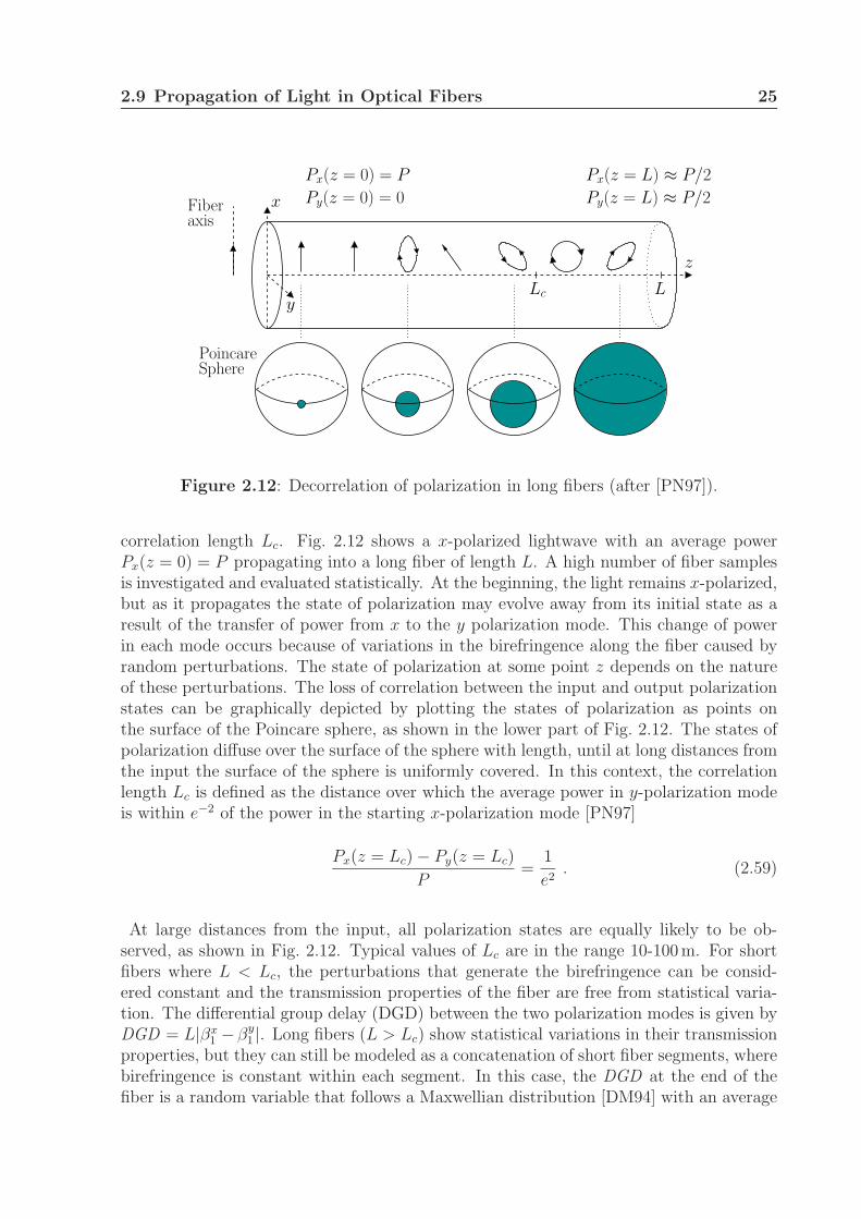
Figure 2.12: Decorrelation of polarization in long fibers (after [PN97]).
correlation length Lc. Fig. 2.12 shows a x-polarized lightwave with an average powerPx(z = 0) = P propagating into a long fiber of length L. A high number of fiber samplesis investigated and evaluated statistically. At the beginning, the light remains x-polarized,but as it propagates the state of polarization may evolve away from its initial state as aresult of the transfer of power from x to the y polarization mode. This change of powerin each mode occurs because of variations in the birefringence along the fiber caused byrandom perturbations. The state of polarization at some point z depends on the natureof these perturbations. The loss of correlation between the input and output polarizationstates can be graphically depicted by plotting the states of polarization as points onthe surface of the Poincare sphere, as shown in the lower part of Fig. 2.12. The states ofpolarization diffuse over the surface of the sphere with length, until at long distances fromthe input the surface of the sphere is uniformly covered. In this context, the correlationlength Lc is defined as the distance over which the average power in y-polarization modeis within e−2 of the power in the starting x-polarization mode [PN97]
Px(z = Lc) − Py(z = Lc)
P=
1
e2. (2.59)
At large distances from the input, all polarization states are equally likely to be ob-served, as shown in Fig. 2.12. Typical values of Lc are in the range 10-100 m. For shortfibers where L < Lc, the perturbations that generate the birefringence can be consid-ered constant and the transmission properties of the fiber are free from statistical varia-tion. The differential group delay (DGD) between the two polarization modes is given byDGD = L|βx
1 −βy1 |. Long fibers (L > Lc) show statistical variations in their transmission
properties, but they can still be modeled as a concatenation of short fiber segments, wherebirefringence is constant within each segment. In this case, the DGD at the end of thefiber is a random variable that follows a Maxwellian distribution [DM94] with an average
26 Chapter 2 ¥ Components of an Optical Communication System
DGD given by
DGD =
√8
3π·√
L · (DPMD)2 , (2.60)
where DPMD is the PMD parameter of the fiber. Note that for short fibers DGD increaseslinearly with distance, while in long fibers DGD increases with the square root of thedistance. Due to its random nature, high DGD values occur in a short period of time,but they often lead to complete system failure. Therefore, fiber-optic communicationsystems are normally designed to operate between moderate and high DGD values inorder to satisfy margin requirements.
2.9.3 Nonlinear Birefringent Fibers
The nonlinearities originating from the third-order susceptibility χ(3) can be included inthe propagation equation by evaluating (2.26) with PNL 6= 0. The dominant part of theinduced electric polarization is PL, which means that PNL can be treated as a first-orderperturbation to PL. If the longitudinal component of the electric field Ez(z, t) is neglected,then E(r, t) can be written as
E(z, t) = Re [xEx(z, t) + yEy(z, t)] , see (2.49)
where
Ex(z, t) = Ax(z, t) exp [j(ω0t − βx0 z)]
Ey(z, t) = Ay(z, t) exp [j(ω0t − βy0z)] .
The last term in (2.43) is due to coherent coupling between the two polarizations andleads to degenerate four-wave mixing. For long fibers (L ≫ Lc), this term can be neglectedbecause it changes sign often and its contribution averages out [MMW97, Agr06]. In thiscase, PNL(z, t) can be written as
PNL(z, t) = ǫ0 ǫNL E(z, t) = ǫ0
[ǫxNL 00 ǫy
NL
]E(z, t) , (2.61)
where
ǫxNL =
3
4χ(3)
xxxx
(|Ex(z, t)|2 +
2
3|Ey(z, t)|2
)ǫyNL =
3
4χ(3)
xxxx
(|Ey(z, t)|2 +
2
3|Ex(z, t)|2
).
The solution of the wave equation (2.26) using (2.61) is generally not possible becauseǫNL is a nonlinear function of the electric fields. However, assuming that ǫNL remainsconstant, a first-order perturbation approach for PNL(z, t) can be used in (2.26). Similarto the linear case, the Helmholtz equation (2.45) can be derived, where the dielectricconstant is given by
ǫ(ω) = 1 + χ(1)xx (ω) + ǫNL . (2.62)
2.9 Propagation of Light in Optical Fibers 27
An intensity dependent refractive index ni(ω) can also be defined as
ni(ω) = ni(ω) + ∆ni , (2.63)
where i ∈ x, y and ∆ni is the nonlinear contribution to the refractive index. Thedielectric constant ǫ(ω) is complex, but due to low optical losses in silica fibers ǫ(ω) canbe taken to be real and replaced by n2(ω). Within this approximation, the nonlinearcontribution to the refractive index can be derived as follows:
ǫi(ω) ≈ n2i (ω) = (ni(ω) + ∆ni)
2
n2i (ω) + ǫi
NL ≈ n2i (ω) + 2ni(ω)∆ni + (∆ni)
2
∆ni ≈ ǫiNL
2 ni(ω)
∆nx = n2(ω0)
(|Ex(z, t)|2 +
2
3|Ey(z, t)|2
)
∆ny = n2(ω0)
(|Ey(z, t)|2 +
2
3|Ex(z, t)|2
) , (2.64)
where
n2(ω0) =3
8n(ω0)Reχ(3)
xxxx
is the nonlinear refractive index and n(ω0) ≈ nx(ω0) ≈ ny(ω0). Although χ(3)xxxx was
already assumed to be real, the real operator Re· was included in order to match thenotation of n2 in textbooks [Agr06]. Finally, the propagation equation describing theevolution of the two polarization components in the fiber can be derived in the same wayas (2.58). This equation is known as the coupled nonlinear Schrodinger equation and isgiven by
∂Ax(z, t)
∂z+ βx
1
∂Ax(z, t)
∂t− j
2β2
∂2Ax(z, t)
∂t2− 1
6β3
∂3Ax(z, t)
∂t3= −α
2Ax(z, t)
−jγ
(|Ax(z, t)|2 +
2
3|Ay(z, t)|2
)Ax(z, t) ,
∂Ay(z, t)
∂z+ βy
1
∂Ay(z, t)
∂t− j
2β2
∂2Ay(z, t)
∂t2− 1
6β3
∂3Ay(z, t)
∂t3= −α
2Ay(z, t)
−jγ
(|Ay(z, t)|2 +
2
3|Ax(z, t)|2
)Ay(z, t)
, (2.65)
where
γ = γ(ω0) =n2(ω0)2π
λ0Aeff
,
28 Chapter 2 ¥ Components of an Optical Communication System
is the nonlinear parameter in (W ·m)−1. If the pulse broadening due to DGD is negligibleand the signal is initialized in a single polarization state, (2.65) can be written as [MMW97]
∂A(z, t)
∂z− j
2β2
∂2A(z, t)
∂t2− 1
6β3
∂3A(z, t)
∂t3= −α
2A(z, t) − jγavg|A(z, t)|2A(z, t) , (2.66)
where γavg is an average value of γ obtained by averaging the nonlinear effects over all
possible states of polarization. In absence of birefringence, γavg = γ, while γavg =8
9γ
for a birefringent fiber. Equation (2.66) is known as the scalar nonlinear Schrodingerequation (NLSE).
2.9.4 Numerical Solutions for the Propagation Equation
As shown in the previous section, the light propagation in optical fibers is subject tovarious linear and nonlinear effects. Depending on the parameters of the transmittedsignal (for example, power and bandwidth), there is a corresponding propagation equation,which models the signal transmission with sufficient accurancy. There are basically threeeffects that determine, which propagation equation should be used in order to match thebalance between simplicity and accuracy:
• birefringence (βx0 6= βy
0 and βx1 6= βy
1 ),
• chromatic dispersion (β2 6= 0 and β3 6= 0) and
• fiber nonlinearity (γ 6= 0).
For instance, considering a fiber of length L, if birefringence and nonlinear effects areneglected, (2.57) can be applied and its solution is given by
A(L, ω) = A(0, ω) · exp
(−α
2L − j
β2ω2
2L − j
β3ω3
6L
). (2.67)
In absence of DGD and chromatic dispersion, (2.66) can be used and simplified by settingβ2 = β3 = 0. The solution is given by
A(L, t) = A(0, t) exp(−α
2L
)exp
(−jγavg|A(0, t)|2Leff
), (2.68)
where Leff = 1−exp(−αL)α
is the effective length of the fiber.
Split-Step Fourier Method
In absence of DGD, (2.66) can accurately model chromatic dispersion and nonlinear ef-fects. This equation is generally difficult to solve analytically, but numerical solution can
2.9 Propagation of Light in Optical Fibers 29
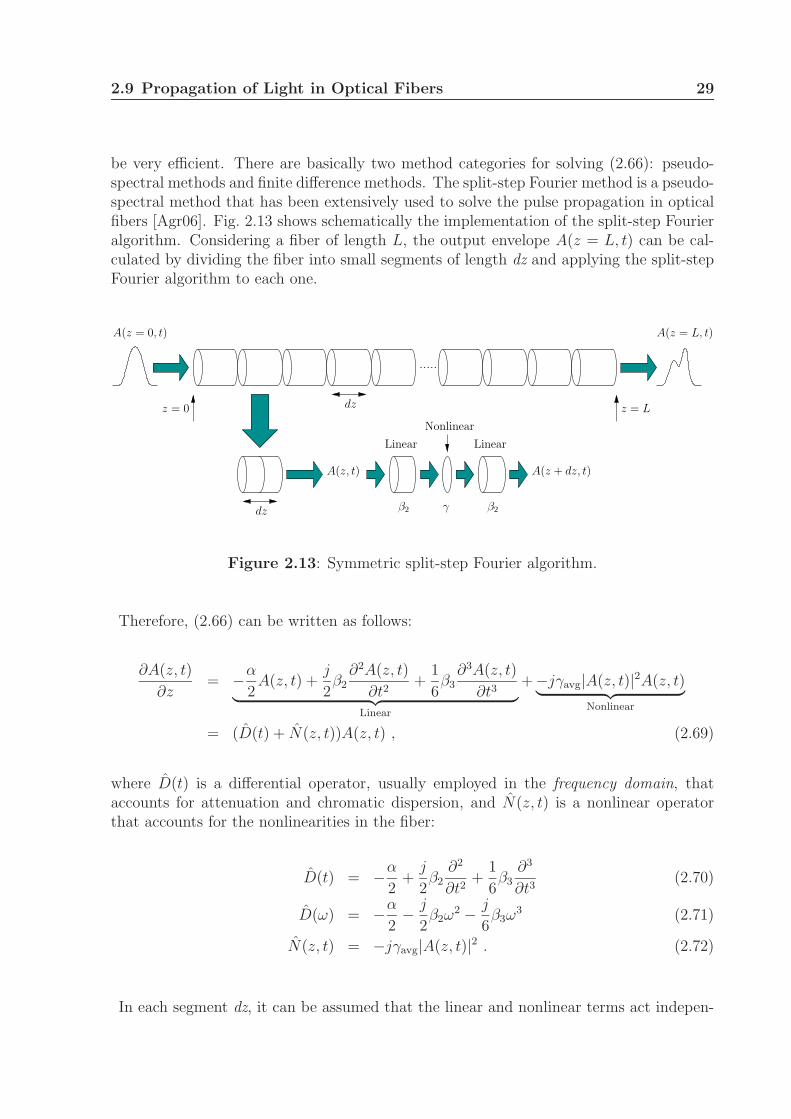
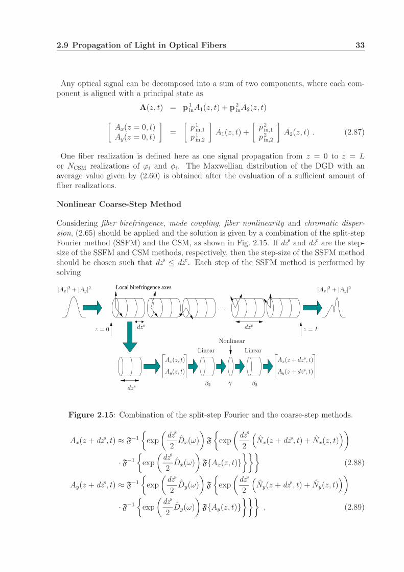
be very efficient. There are basically two method categories for solving (2.66): pseudo-spectral methods and finite difference methods. The split-step Fourier method is a pseudo-spectral method that has been extensively used to solve the pulse propagation in opticalfibers [Agr06]. Fig. 2.13 shows schematically the implementation of the split-step Fourieralgorithm. Considering a fiber of length L, the output envelope A(z = L, t) can be cal-culated by dividing the fiber into small segments of length dz and applying the split-stepFourier algorithm to each one.
z = L
A(z, t) A(z + dz, t)
Nonlinear
Linear Linear
z = 0 dz
dz
A(z = 0, t) A(z = L, t)
β2 γ β2
Figure 2.13: Symmetric split-step Fourier algorithm.
Therefore, (2.66) can be written as follows:
∂A(z, t)
∂z= −α
2A(z, t) +
j
2β2
∂2A(z, t)
∂t2+
1
6β3
∂3A(z, t)
∂t3︸ ︷︷ ︸Linear
+−jγavg|A(z, t)|2A(z, t)︸ ︷︷ ︸Nonlinear
= (D(t) + N(z, t))A(z, t) , (2.69)
where D(t) is a differential operator, usually employed in the frequency domain, thataccounts for attenuation and chromatic dispersion, and N(z, t) is a nonlinear operatorthat accounts for the nonlinearities in the fiber:
D(t) = −α
2+
j
2β2
∂2
∂t2+
1
6β3
∂3
∂t3(2.70)
D(ω) = −α
2− j
2β2ω
2 − j
6β3ω
3 (2.71)
N(z, t) = −jγavg|A(z, t)|2 . (2.72)
In each segment dz, it can be assumed that the linear and nonlinear terms act indepen-
30 Chapter 2 ¥ Components of an Optical Communication System
dently:
∂A
∂z= DA + NA
∂A
A= (D + N)∂z
∫∂A
A=
∫ (D + N
)∂z
ln(A) =
∫ (1
2D + N +
1
2D
)∂z
A(z + dz, t) ≈ F−1
exp
(dz
2D(ω)
)· F
exp
(∫ z+dz
z
N(z′, t)dz′)
·F−1
exp
(dz
2D(ω)
)F A(z, t)
, (2.73)
where F· and F−1· are the direct and inverse Fourier transform operators, respectively.The integral in the previous equation can be evaluated using the trapezoidal formula as
∫ z+dz
z
N(z′, t)dz′ =dz
2(N(z + dz, t) + N(z, t)) . (2.74)
Since N(z + dz, t) depends on A(z + dz, t), the correct solution should be obtained usingan iterative procedure in order to determine A(z + dz, t) from A(z, t).
The step size dz plays an important role in the accuracy of the algorithm. Finding anoptimal step size distribution depends on the parameters of the signal and fiber. There areseveral criteria for choosing the step size dz in the split-step Fourier method [SHZM03].The nonlinear phase rotation method is a variable step-size method and can give accurateresults when nonlinearities are considered. Therefore, for a step of size dz, the effect ofthe nonlinear operator N(z, t) is to increment the phase of A(z, t) by an amount dφNL =dz γavg |A(z, t)|2, where |A(z, t)|2 is the signal’s instantaneous power. An upper bound onthe step size can be obtained by limiting the nonlinear phase increment to a maximumvalue φmax
NL . Moreover, a maximum limit for the step-size dzmax is also set. Thus, dz shouldbe chosen such that
dz ≤ φmaxNL
γ · maxt
[|A(z, t)|2] and dz ≤ dzmax . (2.75)
Coarse-Step Method
In absence of fiber nonlinearity, (2.58) can accurately model birefringence, DGD andchromatic dispersion. In addition, the birefringence axes vary in long fibers leading tomode-coupling, which can be included in (2.58). This equation cannot be solved analyti-cally, but a numerical solution based on the existence of the principal states of polarization
2.9 Propagation of Light in Optical Fibers 31
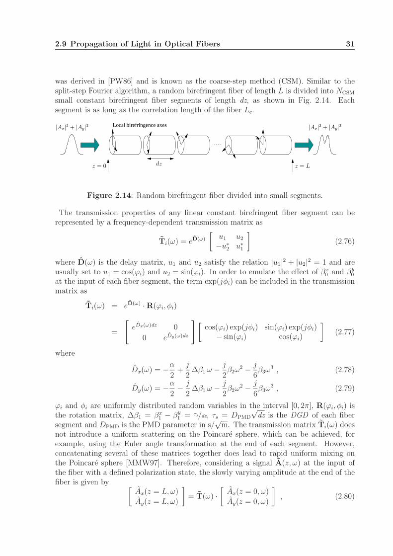
was derived in [PW86] and is known as the coarse-step method (CSM). Similar to thesplit-step Fourier algorithm, a random birefringent fiber of length L is divided into NCSM
small constant birefringent fiber segments of length dz, as shown in Fig. 2.14. Eachsegment is as long as the correlation length of the fiber Lc.
Local birefringence axes |Ax|2 + |Ay|2
dz z = Lz = 0
|Ax|2 + |Ay|2
Figure 2.14: Random birefringent fiber divided into small segments.
The transmission properties of any linear constant birefringent fiber segment can berepresented by a frequency-dependent transmission matrix as
Ti(ω) = eD(ω)
[u1 u2
−u∗2 u∗
1
](2.76)
where D(ω) is the delay matrix, u1 and u2 satisfy the relation |u1|2 + |u2|2 = 1 and areusually set to u1 = cos(ϕi) and u2 = sin(ϕi). In order to emulate the effect of βx
0 and βy0
at the input of each fiber segment, the term exp(jφi) can be included in the transmissionmatrix as
Ti(ω) = eD(ω) · R(ϕi, φi)
=
[eDx(ω)dz 0
0 eDy(ω)dz
] [cos(ϕi) exp(jφi) sin(ϕi) exp(jφi)
− sin(ϕi) cos(ϕi)
](2.77)
where
Dx(ω) = −α
2+
j
2∆β1 ω − j
2β2ω
2 − j
6β3ω
3 , (2.78)
Dy(ω) = −α
2− j
2∆β1 ω − j
2β2ω
2 − j
6β3ω
3 , (2.79)
ϕi and φi are uniformly distributed random variables in the interval [0, 2π], R(ϕi, φi) isthe rotation matrix, ∆β1 = βx
1 − βy1 = τs/dz, τs = DPMD
√dz is the DGD of each fiber
segment and DPMD is the PMD parameter in s/√
m. The transmission matrix Ti(ω) doesnot introduce a uniform scattering on the Poincare sphere, which can be achieved, forexample, using the Euler angle transformation at the end of each segment. However,concatenating several of these matrices together does lead to rapid uniform mixing onthe Poincare sphere [MMW97]. Therefore, considering a signal A(z, ω) at the input ofthe fiber with a defined polarization state, the slowly varying amplitude at the end of thefiber is given by [
Ax(z = L, ω)
Ay(z = L, ω)
]= T(ω) ·
[Ax(z = 0, ω)
Ay(z = 0, ω)
], (2.80)
32 Chapter 2 ¥ Components of an Optical Communication System
where
T(ω) =
NCSM∏
i=1
Ti(ω) .
The principal states model is based on the observation that for any transmission matrixT(ω) there exists at every frequency an orthogonal pair of input principal states of polar-ization (PSP) [PW86, PN97]. If an optical signal is aligned with one of the PSP’s at theinput of the fiber, it will emerge at the output with its spectral components all having thesame state of polarization (polarized) and also undistorted to the first order. The PSP’sat the input of the fiber are obtained using the following eigenvalue equation [PW86]:
(T−1(ω)
∂T(ω)
∂ω
)· Pin = jρ · Pin , (2.81)
where “ω” is the frequency in baseband, the matrix Pin contains the two PSP’s and isgiven by
Pin =[p 1
in p 2in
]=
[p 1
in,1 p 2in,1
p 1in,2 p 2
in,2
]. (2.82)
Since T(ω) is a unitary matrix, then T−1(ω) = TH(ω). Using the approximation [Hef92]
∂T(ω)
∂ω≈ T(ω + δω) − T(ω)
δω,
the eigenvalue equation can be written as(TH(ω) T(ω + δω)
)· Pin = (1 + j ρ δω)︸ ︷︷ ︸
ρ′
·Pin . (2.83)
where δω is a small frequency increment. Using (2.83), the DGD at the frequency ω isgiven by
DGD |ω =Im ρ′
1 − ρ′2
δω, (2.84)
where ρ′1 and ρ′
2 are the eigenvalues obtained after eigendecomposition of the matrixTH(ω) T(ω + δω). For an optical modulated signal, the DGD is usually calculated at thecarrier frequency ω0. Since ω is given in baseband, then the carrier frequency correspondsto ω = 0. In this case, the matrix TH(ω) T(ω + δω) is given by
TH(0) T(δω) =
(NCSM∏
i=1
R(ϕi, φi)
)H
·NCSM∏
i=1
[ej δω τs
2 00 e−j δω τs
2
]· R(ϕi, φi) , (2.85)
Note that the parameters α, β2 and β3 do not affect the evaluation of the PSP’s andDGD, because they can be taken out of the matrix D(ω) and will cancel out in (2.83).The PSP’s at the output of the fiber Pout can be obtained using the following equation:
Pout = T(ω)Pin . (2.86)
2.9 Propagation of Light in Optical Fibers 33
Any optical signal can be decomposed into a sum of two components, where each com-ponent is aligned with a principal state as
A(z, t) = p 1inA1(z, t) + p 2
inA2(z, t)
[Ax(z = 0, t)Ay(z = 0, t)
]=
[p 1
in,1
p 1in,2
]A1(z, t) +
[p 2
in,1
p 2in,2
]A2(z, t) . (2.87)
One fiber realization is defined here as one signal propagation from z = 0 to z = Lor NCSM realizations of ϕi and φi. The Maxwellian distribution of the DGD with anaverage value given by (2.60) is obtained after the evaluation of a sufficient amount offiber realizations.
Nonlinear Coarse-Step Method
Considering fiber birefringence, mode coupling, fiber nonlinearity and chromatic disper-sion, (2.65) should be applied and the solution is given by a combination of the split-stepFourier method (SSFM) and the CSM, as shown in Fig. 2.15. If dzs and dzc are the step-size of the SSFM and CSM methods, respectively, then the step-size of the SSFM methodshould be chosen such that dzs ≤ dzc. Each step of the SSFM method is performed bysolving
Local birefringence axes
Ay(z + dzs, t)Ay(z, t)
Ax(z, t)
Nonlinear
Linear Linear
β2 γ β2
Ax(z + dzs, t)
z = Lz = 0
|Ax|2 + |Ay|2 |Ax|2 + |Ay|2
dzs dzc
dzs
Figure 2.15: Combination of the split-step Fourier and the coarse-step methods.
Ax(z + dzs, t) ≈ F−1
exp
(dzs
2Dx(ω)
)F
exp
(dzs
2
(Nx(z + dzs, t) + Nx(z, t)
))
·F−1
exp
(dzs
2Dx(ω)
)FAx(z, t)
(2.88)
Ay(z + dzs, t) ≈ F−1
exp
(dzs
2Dy(ω)
)F
exp
(dzs
2
(Ny(z + dzs, t) + Ny(z, t)
))
·F−1
exp
(dzs
2Dy(ω)
)FAy(z, t)
, (2.89)
34 Chapter 2 ¥ Components of an Optical Communication System
where
Nx(z, t) = −jγ
(|Ax(z, t)|2 +
2
3|Ay(z, t)|2
), (2.90)
Ny(z, t) = −jγ
(|Ay(z, t)|2 +
2
3|Ax(z, t)|2
), (2.91)
and Dx(ω) and Dy(ω) are given by (2.78) and (2.79), respectively. During the propagation,the birefringent axes should be rotated at the points (i−1)·dzc, where i ∈ 1, 2, . . . , NCSM,according to the equation
[Ax(z = (i − 1) · dzc, ω)
Ay(z = (i − 1) · dzc, ω)
]new
= R(ϕi, φi) ·[
Ax(z = (i − 1) · dzc, ω)
Ay(z = (i − 1) · dzc, ω)
]old
, (2.92)
in order to simulate random perturbations and mode-coupling of the fiber.
2.10 Summary
The main components of an optical communication system were introduced in this chap-ter. The focus was put on the modeling and simulation of single-channel long-haul sys-tems. First, the generation of the electrical signal carrying the information was modeledusing pseudo-random sequences and pulse shaping. The processes involving the generationof light was briefly discussed and the laser was shown to be the most appropriate opticalsource for long-haul fiber-optic communication systems. In order to efficiently modulatethe electrical signal into the optical carrier, the theory and operation of Mach-Zehndermodulators (MZM) were described in detail. Propagation losses are compensated by op-tical amplifiers, where different amplifier strategies were discussed, but only the EDFA,which is commonly used in WDM networks, was treated in detail. Finally, the propaga-tion equation of the light in a single-mode fiber and its numerical solution were derivedconsidering several linear and nonlinear effects.
3Modulation Formats
Modulation is the process of varying one or more parameters of an optical carrier inaccordance with the information signal. The choice of one or more parameters, which aregoing to be modulated determines the modulation format. The optical carrier wave isgiven by
E(t) = Ree · |A|ejϕ · ej·ω·t = Ree · E(t) , (3.1)
where E(t) is the electrical field vector, e is the polarization unit vector, A is the slowlyvarying complex amplitude, ϕ is the phase of A and ω is the carrier frequency. The mod-ulation of anyone of these four parameters (e, |A|, ω, ϕ) results in four basic modulationtechniques: polarization-shift keying (PolSK), amplitude-shift keying (ASK), frequency-shift keying (FSK) and phase-shift keying (PSK), respectively. In fiber-optic communica-tions, PolSK and FSK are not commonly used and will not be considered in this thesis.Therefore, ω = ω0 is assumed and e is constant at the transmitter, but it may vary duringthe propagation in the fiber. In the following sections, different implementations of ASK,PSK and a combination of both will be investigated as well as stereo multiplexing.
3.1 Amplitude Shift Keying
Binary amplitude shift keying is the most common modulation format in optical com-munication systems mainly because of its simplicity in modulating and demodulating.Due to the intensity changes between two levels, where one is set to zero, it is oftencalled On-Off keying (OOK). Although more than two levels are possible, the large re-ceiver sensitivity penalty compared to binary ASK [WE08] limits its use in fiber-opticcommunication systems. The transmitter model and signal constellation for binary ASKare shown in Fig. 3.1. The MZM 1 is the pulse carver and is used to generate a train
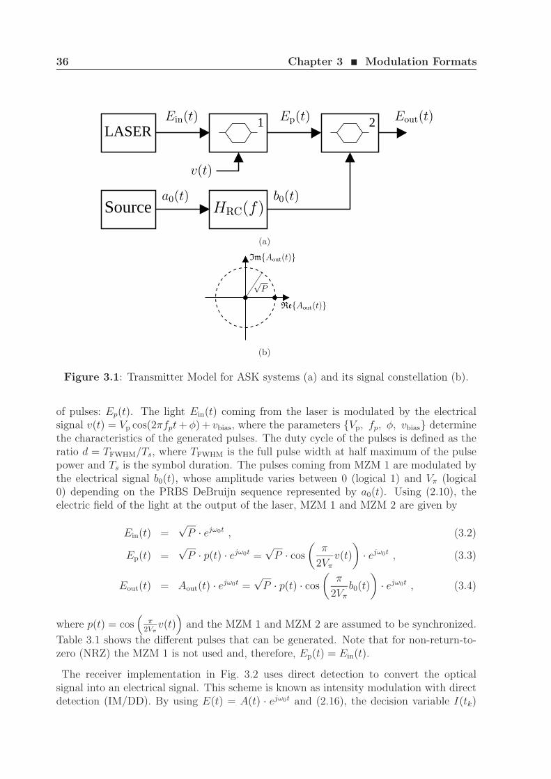
36 Chapter 3 ¥ Modulation Formats
LASER
Source
1 2
HRC(f)a0(t) b0(t)
v(t)
Ein(t) Ep(t) Eout(t)
(a)
√P
ReAout(t)
ImAout(t)
(b)
Figure 3.1: Transmitter Model for ASK systems (a) and its signal constellation (b).
of pulses: Ep(t). The light Ein(t) coming from the laser is modulated by the electricalsignal v(t) = Vp cos(2πfpt + φ) + vbias, where the parameters Vp, fp, φ, vbias determinethe characteristics of the generated pulses. The duty cycle of the pulses is defined as theratio d = TFWHM/Ts, where TFWHM is the full pulse width at half maximum of the pulsepower and Ts is the symbol duration. The pulses coming from MZM 1 are modulated bythe electrical signal b0(t), whose amplitude varies between 0 (logical 1) and Vπ (logical0) depending on the PRBS DeBruijn sequence represented by a0(t). Using (2.10), theelectric field of the light at the output of the laser, MZM 1 and MZM 2 are given by
Ein(t) =√
P · ejω0t , (3.2)
Ep(t) =√
P · p(t) · ejω0t =√
P · cos
(π
2Vπ
v(t)
)· ejω0t , (3.3)
Eout(t) = Aout(t) · ejω0t =√
P · p(t) · cos
(π
2Vπ
b0(t)
)· ejω0t , (3.4)
where p(t) = cos(
π2Vπ
v(t))
and the MZM 1 and MZM 2 are assumed to be synchronized.
Table 3.1 shows the different pulses that can be generated. Note that for non-return-to-zero (NRZ) the MZM 1 is not used and, therefore, Ep(t) = Ein(t).
The receiver implementation in Fig. 3.2 uses direct detection to convert the opticalsignal into an electrical signal. This scheme is known as intensity modulation with directdetection (IM/DD). By using E(t) = A(t) · ejω0t and (2.16), the decision variable I(tk)
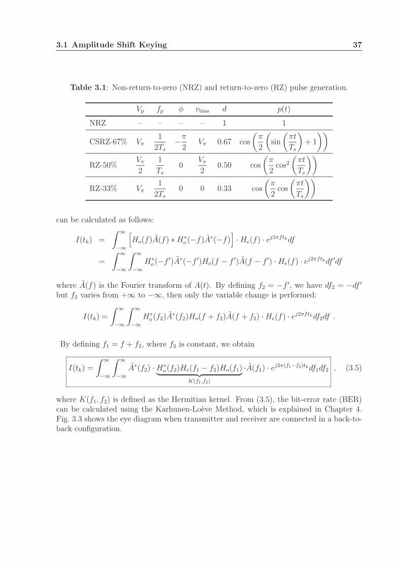
3.1 Amplitude Shift Keying 37
Table 3.1: Non-return-to-zero (NRZ) and return-to-zero (RZ) pulse generation.
Vp fp φ vbias d p(t)
NRZ – – – – 1 1
CSRZ-67% Vπ
1
2Ts
−π
2Vπ 0.67 cos
(π
2
(sin
(πt
Ts
)+ 1
))
RZ-50%Vπ
2
1
Ts
0Vπ
20.50 cos
(π
2cos2
(πt
Ts
))
RZ-33% Vπ
1
2Ts
0 0 0.33 cos
(π
2cos
(πt
Ts
))
can be calculated as follows:
I(tk) =
∫ ∞
−∞
[Ho(f)A(f) ∗ H∗
o (−f)A∗(−f)]· He(f) · ej2πftkdf
=
∫ ∞
−∞
∫ ∞
−∞H∗
o (−f ′)A∗(−f ′)Ho(f − f ′)A(f − f ′) · He(f) · ej2πftkdf ′df
where A(f) is the Fourier transform of A(t). By defining f2 = −f ′, we have df2 = −df ′
but f2 varies from +∞ to −∞, then only the variable change is performed:
I(tk) =
∫ ∞
−∞
∫ ∞
−∞H∗
o (f2)A∗(f2)Ho(f + f2)A(f + f2) · He(f) · ej2πftkdf2df .
By defining f1 = f + f2, where f2 is constant, we obtain
I(tk) =
∫ ∞
−∞
∫ ∞
−∞A∗(f2) · H∗
o (f2)He(f1 − f2)Ho(f1)︸ ︷︷ ︸K(f1,f2)
·A(f1) · ej2π(f1−f2)tkdf1df2 , (3.5)
where K(f1, f2) is defined as the Hermitian kernel. From (3.5), the bit-error rate (BER)can be calculated using the Karhunen-Loeve Method, which is explained in Chapter 4.Fig. 3.3 shows the eye diagram when transmitter and receiver are connected in a back-to-back configuration.
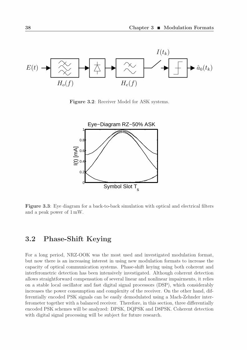
38 Chapter 3 ¥ Modulation Formats
Ho(f)
I(tk)
E(t) a0(tk)
He(f)
Figure 3.2: Receiver Model for ASK systems.
0
0.2
0.4
0.6
0.8
1
Symbol Slot Ts
I(t)
[mA
]
Eye−Diagram RZ−50% ASK
Figure 3.3: Eye diagram for a back-to-back simulation with optical and electrical filtersand a peak power of 1 mW.
3.2 Phase-Shift Keying
For a long period, NRZ-OOK was the most used and investigated modulation format,but now there is an increasing interest in using new modulation formats to increase thecapacity of optical communication systems. Phase-shift keying using both coherent andinterferometric detection has been intensively investigated. Although coherent detectionallows straightforward compensation of several linear and nonlinear impairments, it relieson a stable local oscillator and fast digital signal processors (DSP), which considerablyincreases the power consumption and complexity of the receiver. On the other hand, dif-ferentially encoded PSK signals can be easily demodulated using a Mach-Zehnder inter-ferometer together with a balanced receiver. Therefore, in this section, three differentiallyencoded PSK schemes will be analyzed: DPSK, DQPSK and D8PSK. Coherent detectionwith digital signal processing will be subject for future research.
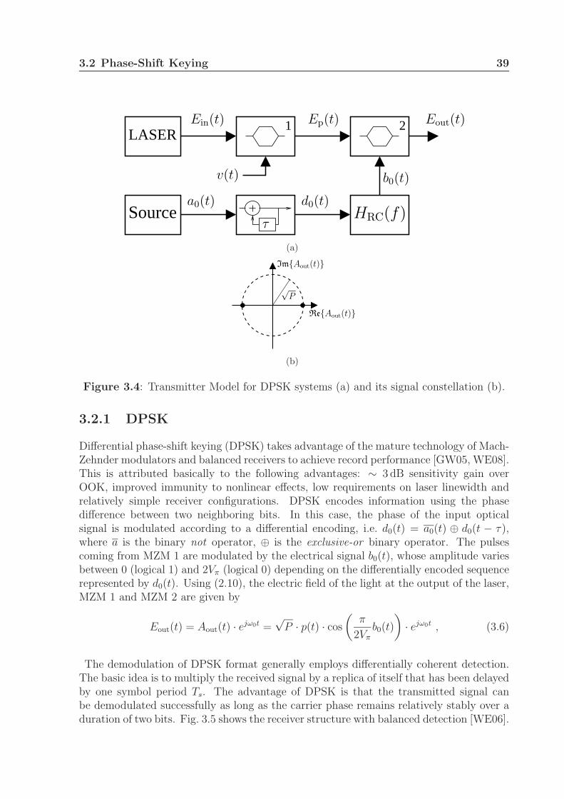
3.2 Phase-Shift Keying 39
LASER
Source
1 2
HRC(f)τ
a0(t)
v(t)
Ein(t) Ep(t) Eout(t)
b0(t)
d0(t)
(a)
√P
ReAout(t)
ImAout(t)
(b)
Figure 3.4: Transmitter Model for DPSK systems (a) and its signal constellation (b).
3.2.1 DPSK
Differential phase-shift keying (DPSK) takes advantage of the mature technology of Mach-Zehnder modulators and balanced receivers to achieve record performance [GW05, WE08].This is attributed basically to the following advantages: ∼ 3 dB sensitivity gain overOOK, improved immunity to nonlinear effects, low requirements on laser linewidth andrelatively simple receiver configurations. DPSK encodes information using the phasedifference between two neighboring bits. In this case, the phase of the input opticalsignal is modulated according to a differential encoding, i.e. d0(t) = a0(t) ⊕ d0(t − τ),where a is the binary not operator, ⊕ is the exclusive-or binary operator. The pulsescoming from MZM 1 are modulated by the electrical signal b0(t), whose amplitude variesbetween 0 (logical 1) and 2Vπ (logical 0) depending on the differentially encoded sequencerepresented by d0(t). Using (2.10), the electric field of the light at the output of the laser,MZM 1 and MZM 2 are given by
Eout(t) = Aout(t) · ejω0t =√
P · p(t) · cos
(π
2Vπ
b0(t)
)· ejω0t , (3.6)
The demodulation of DPSK format generally employs differentially coherent detection.The basic idea is to multiply the received signal by a replica of itself that has been delayedby one symbol period Ts. The advantage of DPSK is that the transmitted signal canbe demodulated successfully as long as the carrier phase remains relatively stably over aduration of two bits. Fig. 3.5 shows the receiver structure with balanced detection [WE06].
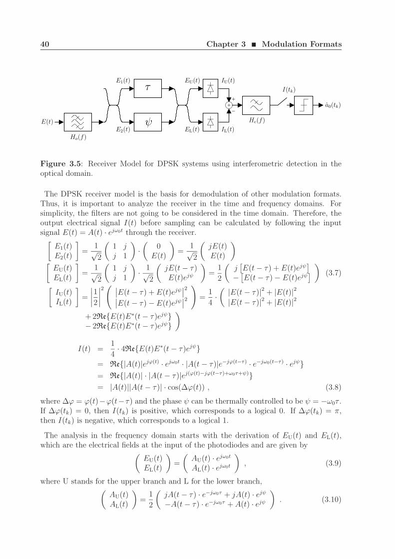
40 Chapter 3 ¥ Modulation Formats
IL(t)
I(tk)
Ho(f)
He(f)
a0(tk)
E(t)
τ
ψ
EU(t)
EL(t)
E1(t)
E2(t)
IU(t)
Figure 3.5: Receiver Model for DPSK systems using interferometric detection in theoptical domain.
The DPSK receiver model is the basis for demodulation of other modulation formats.Thus, it is important to analyze the receiver in the time and frequency domains. Forsimplicity, the filters are not going to be considered in the time domain. Therefore, theoutput electrical signal I(t) before sampling can be calculated by following the inputsignal E(t) = A(t) · ejω0t through the receiver.
[E1(t)E2(t)
]=
1√2
(1 jj 1
)·(
0E(t)
)=
1√2
(jE(t)E(t)
)
[EU(t)EL(t)
]=
1√2
(1 jj 1
)· 1√
2
(jE(t − τ)E(t)ejψ
)=
1
2
(j[E(t − τ) + E(t)ejψ
]
−[E(t − τ) − E(t)ejψ
])
(3.7)
[IU(t)IL(t)
]=
∣∣∣∣1
2
∣∣∣∣2( ∣∣E(t − τ) + E(t)ejψ
∣∣2∣∣E(t − τ) − E(t)ejψ
∣∣2
)=
1
4·(
|E(t − τ)|2 + |E(t)|2|E(t − τ)|2 + |E(t)|2
+ 2ReE(t)E∗(t − τ)ejψ− 2ReE(t)E∗(t − τ)ejψ
)
I(t) =1
4· 4ReE(t)E∗(t − τ)ejψ
= Re|A(t)|ejϕ(t) · ejω0t · |A(t − τ)|e−jϕ(t−τ) · e−jω0(t−τ) · ejψ= Re|A(t)| · |A(t − τ)|ej(ϕ(t)−jϕ(t−τ)+ω0τ+ψ)= |A(t)||A(t − τ)| · cos(∆ϕ(t)) , (3.8)
where ∆ϕ = ϕ(t)−ϕ(t−τ) and the phase ψ can be thermally controlled to be ψ = −ω0τ .If ∆ϕ(tk) = 0, then I(tk) is positive, which corresponds to a logical 0. If ∆ϕ(tk) = π,then I(tk) is negative, which corresponds to a logical 1.
The analysis in the frequency domain starts with the derivation of EU(t) and EL(t),which are the electrical fields at the input of the photodiodes and are given by
(EU(t)EL(t)
)=
(AU(t) · ejω0t
AL(t) · ejω0t
), (3.9)
where U stands for the upper branch and L for the lower branch,(
AU(t)AL(t)
)=
1
2
(jA(t − τ) · e−jω0τ + jA(t) · ejψ
−A(t − τ) · e−jω0τ + A(t) · ejψ
). (3.10)
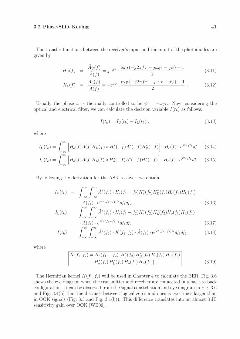
3.2 Phase-Shift Keying 41
The transfer functions between the receiver’s input and the input of the photodiodes aregiven by
HU(f) =AU(f)
A(f)= j ejψ · exp (−j2πfτ − jω0τ − jψ) + 1
2(3.11)
HL(f) =AL(f)
A(f)= −ejψ · exp (−j2πfτ − jω0τ − jψ) − 1
2. (3.12)
Usually the phase ψ is thermally controlled to be ψ = −ω0τ . Now, considering theoptical and electrical filter, we can calculate the decision variable I(tk) as follows:
I(tk) = IU(tk) − IL(tk) , (3.13)
where
IU(tk) =
∫ ∞
−∞
[Ho(f)A(f)HU(f) ∗ H∗
o (−f)A∗(−f)H∗U(−f)
]· He(f) · ej2πftkdf (3.14)
IL(tk) =
∫ ∞
−∞
[Ho(f)A(f)HL(f) ∗ H∗
o (−f)A∗(−f)H∗L(−f)
]· He(f) · ej2πftkdf . (3.15)
By following the derivation for the ASK receiver, we obtain
IU(tk) =
∫ ∞
−∞
∫ ∞
−∞A∗(f2) · He(f1 − f2)H
∗o (f2)H
∗U(f2)Ho(f1)HU(f1)
· A(f1) · ej2π(f1−f2)tkdf1df2 (3.16)
IL(tk) =
∫ ∞
−∞
∫ ∞
−∞A∗(f2) · He(f1 − f2)H
∗o (f2)H
∗L(f2)Ho(f1)HL(f1)
· A(f1) · ej2π(f1−f2)tkdf1df2 (3.17)
I(tk) =
∫ ∞
−∞
∫ ∞
−∞A∗(f2) · K(f1, f2) · A(f1) · ej2π(f1−f2)tkdf1df2 , (3.18)
where
K(f1, f2) = He(f1 − f2) [H∗o (f2) H∗
U(f2) Ho(f1) HU(f1)
−H∗o (f2) H∗
L(f2) Ho(f1) HL(f1)] . (3.19)
The Hermitian kernel K(f1, f2) will be used in Chapter 4 to calculate the BER. Fig. 3.6shows the eye diagram when the transmitter and receiver are connected in a back-to-backconfiguration. It can be observed from the signal constellation and eye diagram in Fig. 3.6and Fig. 3.4(b) that the distance between logical zeros and ones is two times larger thanin OOK signals (Fig. 3.3 and Fig. 3.1(b)). This difference translates into an almost 3 dBsensitivity gain over OOK [WE06].
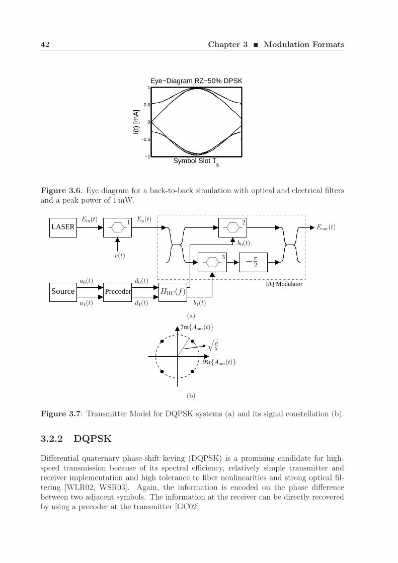
42 Chapter 3 ¥ Modulation Formats
−1
−0.5
0
0.5
1
Symbol Slot Ts
I(t)
[mA
]
Eye−Diagram RZ−50% DPSK
Figure 3.6: Eye diagram for a back-to-back simulation with optical and electrical filtersand a peak power of 1 mW.
3
2
Source Precoder
LASER1
I/Q ModulatorHRC(f)
a0(t)
a1(t)
d0(t)
d1(t)
Ein(t)
v(t) −π2
b0(t)
Ep(t)
b1(t)
Eout(t)
(a)
√P2
ImAout(t)
ReAout(t)
(b)
Figure 3.7: Transmitter Model for DQPSK systems (a) and its signal constellation (b).
3.2.2 DQPSK
Differential quaternary phase-shift keying (DQPSK) is a promising candidate for high-speed transmission because of its spectral efficiency, relatively simple transmitter andreceiver implementation and high tolerance to fiber nonlinearities and strong optical fil-tering [WLR02, WSR03]. Again, the information is encoded on the phase differencebetween two adjacent symbols. The information at the receiver can be directly recoveredby using a precoder at the transmitter [GC02].
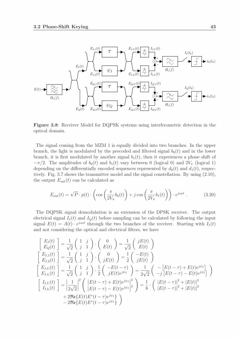
3.2 Phase-Shift Keying 43
II,U(t)II(tk)
a0(tk)
Ho(f)
E(t)
τ
He(f)ψIEI(t)
EI,1(t)
EI,2(t)
EI,U(t)
EI,L(t)
IQ(tk)
a1(tk)
τ
He(f)ψQ
EQ,1(t)
EQ,2(t)EQ(t)
EQ,U(t)
EQ,L(t)
II,L(t)
IQ,U(t)
IQ,L(t)
Figure 3.8: Receiver Model for DQPSK systems using interferometric detection in theoptical domain.
The signal coming from the MZM 1 is equally divided into two branches. In the upperbranch, the light is modulated by the precoded and filtered signal b0(t) and in the lowerbranch, it is first modulated by another signal b1(t), then it experiences a phase shift of−π/2. The amplitudes of b0(t) and b1(t) vary between 0 (logical 0) and 2Vπ (logical 1)depending on the differentially encoded sequences represented by d0(t) and d1(t), respec-tively. Fig. 3.7 shows the transmitter model and the signal constellation. By using (2.10),the output Eout(t) can be calculated as
Eout(t) =√
P · p(t) ·(
cos
(π
2Vπ
b0(t)
)+ j cos
(π
2Vπ
b1(t)
))· ejω0t . (3.20)
The DQPSK signal demodulation is an extension of the DPSK receiver. The outputelectrical signal II(t) and IQ(t) before sampling can be calculated by following the inputsignal E(t) = A(t) · ejω0t through the two branches of the receiver. Starting with II(t)and not considering the optical and electrical filters, we have
[EI(t)EQ(t)
]=
1√2
(1 jj 1
)·(
0E(t)
)=
1√2
(jE(t)E(t)
)
[EI,1(t)EI,2(t)
]=
1√2
(1 jj 1
)·(
0jE(t)
)=
1
2
(−E(t)jE(t)
)
[EI,U(t)EI,L(t)
]=
1√2
(1 jj 1
)· 1
2
(−E(t − τ)jE(t)ejψI
)=
1
2√
2
(−
[E(t − τ) + E(t)ejψI
]
−j[E(t − τ) − E(t)ejψI
])
[II,U(t)II,L(t)
]=
∣∣∣∣1
2√
2
∣∣∣∣2( ∣∣E(t − τ) + E(t)ejψI
∣∣2∣∣E(t − τ) − E(t)ejψI
∣∣2
)=
1
8·(
|E(t − τ)|2 + |E(t)|2|E(t − τ)|2 + |E(t)|2
+ 2ReE(t)E∗(t − τ)ejψI− 2ReE(t)E∗(t − τ)ejψI
)
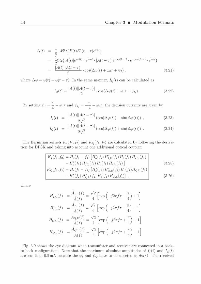
44 Chapter 3 ¥ Modulation Formats
II(t) =1
8· 4ReE(t)E∗(t − τ)ejψI
=1
2Re|A(t)|ejϕ(t) · ejω0t · |A(t − τ)|e−jϕ(t−τ) · e−jω0(t−τ) · ejψI
=|A(t)||A(t − τ)|
2· cos(∆ϕ(t) + ω0τ + ψI) , (3.21)
where ∆ϕ = ϕ(t) − ϕ(t − τ). In the same manner, IQ(t) can be calculated as
IQ(t) =|A(t)||A(t − τ)|
2· cos(∆ϕ(t) + ω0τ + ψQ) . (3.22)
By setting ψI =π
4− ω0τ and ψQ = −π
4− ω0τ , the decision currents are given by
II(t) =|A(t)||A(t − τ)|
2√
2(cos(∆ϕ(t)) − sin(∆ϕ(t))) , (3.23)
IQ(t) =|A(t)||A(t − τ)|
2√
2(cos(∆ϕ(t)) + sin(∆ϕ(t))) . (3.24)
The Hermitian kernels KI(f1, f2) and KQ(f1, f2) are calculated by following the deriva-tion for DPSK and taking into account one additional optical coupler:
KI(f1, f2) = He(f1 − f2)[H∗
o (f2) H∗I,U(f2) Ho(f1) HI,U(f1)
−H∗o (f2) H∗
I,L(f2) Ho(f1) HI,L(f1)]
KQ(f1, f2) = He(f1 − f2)[H∗
o (f2) H∗Q,U(f2) Ho(f1)HQ,U(f1)
−H∗o (f2) H∗
Q,L(f2) Ho(f1) HQ,L(f1)]
,
(3.25)
(3.26)
where
HI,U(f) =AI,U(f)
A(f)=
√2
4
[exp
(−j2πfτ − π
4
)+ 1
]
HI,L(f) =AI,L(f)
A(f)=
√2
4
[exp
(−j2πfτ − π
4
)− 1
]
HQ,U(f) =AQ,U(f)
A(f)=
√2
4
[exp
(−j2πfτ +
π
4
)+ 1
]
HQ,L(f) =AQ,L(f)
A(f)=
√2
4
[exp
(−j2πfτ +
π
4
)− 1
]
Fig. 3.9 shows the eye diagram when transmitter and receiver are connected in a back-to-back configuration. Note that the maximum absolute amplitudes of II(t) and IQ(t)are less than 0.5 mA because the ψI and ψQ have to be selected as ±π/4. The received
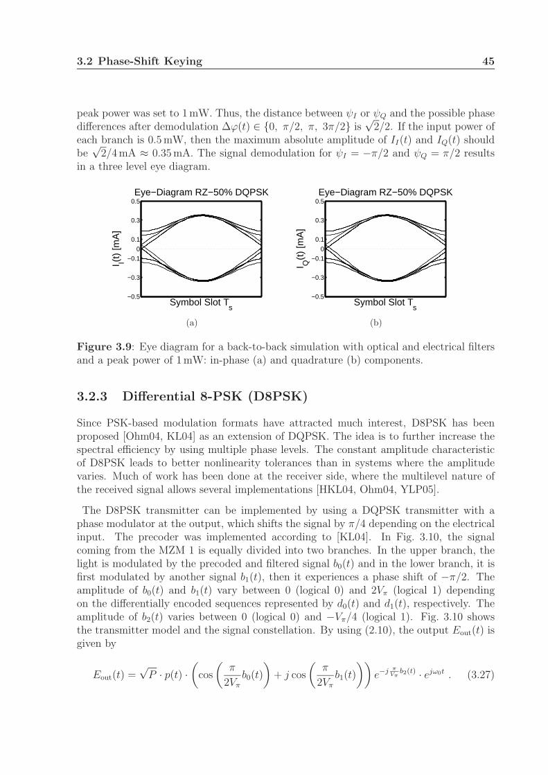
3.2 Phase-Shift Keying 45
peak power was set to 1 mW. Thus, the distance between ψI or ψQ and the possible phasedifferences after demodulation ∆ϕ(t) ∈ 0, π/2, π, 3π/2 is
√2/2. If the input power of
each branch is 0.5 mW, then the maximum absolute amplitude of II(t) and IQ(t) shouldbe
√2/4 mA ≈ 0.35 mA. The signal demodulation for ψI = −π/2 and ψQ = π/2 results
in a three level eye diagram.
−0.5
−0.3
−0.1
0
0.1
0.3
0.5
Symbol Slot Ts
I I(t)
[mA
]
Eye−Diagram RZ−50% DQPSK
(a)
−0.5
−0.3
−0.1
0
0.1
0.3
0.5
Symbol Slot Ts
I Q(t
) [m
A]
Eye−Diagram RZ−50% DQPSK
(b)
Figure 3.9: Eye diagram for a back-to-back simulation with optical and electrical filtersand a peak power of 1 mW: in-phase (a) and quadrature (b) components.
3.2.3 Differential 8-PSK (D8PSK)
Since PSK-based modulation formats have attracted much interest, D8PSK has beenproposed [Ohm04, KL04] as an extension of DQPSK. The idea is to further increase thespectral efficiency by using multiple phase levels. The constant amplitude characteristicof D8PSK leads to better nonlinearity tolerances than in systems where the amplitudevaries. Much of work has been done at the receiver side, where the multilevel nature ofthe received signal allows several implementations [HKL04, Ohm04, YLP05].
The D8PSK transmitter can be implemented by using a DQPSK transmitter with aphase modulator at the output, which shifts the signal by π/4 depending on the electricalinput. The precoder was implemented according to [KL04]. In Fig. 3.10, the signalcoming from the MZM 1 is equally divided into two branches. In the upper branch, thelight is modulated by the precoded and filtered signal b0(t) and in the lower branch, it isfirst modulated by another signal b1(t), then it experiences a phase shift of −π/2. Theamplitude of b0(t) and b1(t) vary between 0 (logical 0) and 2Vπ (logical 1) dependingon the differentially encoded sequences represented by d0(t) and d1(t), respectively. Theamplitude of b2(t) varies between 0 (logical 0) and −Vπ/4 (logical 1). Fig. 3.10 showsthe transmitter model and the signal constellation. By using (2.10), the output Eout(t) isgiven by
Eout(t) =√
P · p(t) ·(
cos
(π
2Vπ
b0(t)
)+ j cos
(π
2Vπ
b1(t)
))e−j π
Vπb2(t) · ejω0t . (3.27)
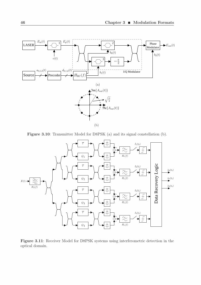
46 Chapter 3 ¥ Modulation Formats
3
2
Source Precoder
LASER1
I/Q Modulator
PhaseModulator
HRC(f)
a0,1,2(t) d0,1,2(t)
Ein(t)
v(t) −π2
b0(t)
Ep(t)
b1(t)
b2(t)
Eout(t)
(a)
ImAout(t)
ReAout(t)
√P2
(b)
Figure 3.10: Transmitter Model for D8PSK (a) and its signal constellation (b).
Dat
a R
ecov
ery
Logi
c
ψ4
I2(tk)τ
I1(tk)τ
I4(tk)τ
I3(tk)τ
a0(tk)
a1(tk)
a2(tk)
E(t)
He(f)
He(f)
He(f)
He(f)
Ho(f)
ψ1
ψ2
ψ3
Figure 3.11: Receiver Model for D8PSK systems using interferometric detection in theoptical domain.
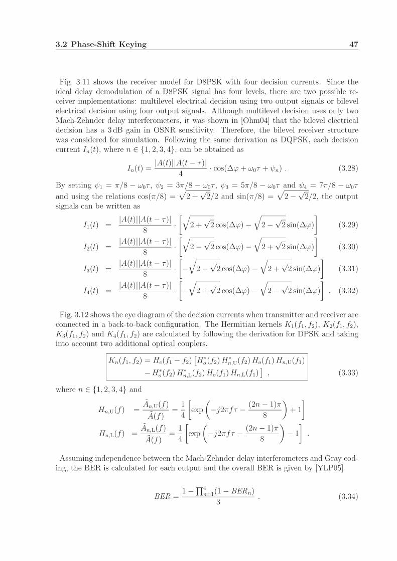
3.2 Phase-Shift Keying 47
Fig. 3.11 shows the receiver model for D8PSK with four decision currents. Since theideal delay demodulation of a D8PSK signal has four levels, there are two possible re-ceiver implementations: multilevel electrical decision using two output signals or bilevelelectrical decision using four output signals. Although multilevel decision uses only twoMach-Zehnder delay interferometers, it was shown in [Ohm04] that the bilevel electricaldecision has a 3 dB gain in OSNR sensitivity. Therefore, the bilevel receiver structurewas considered for simulation. Following the same derivation as DQPSK, each decisioncurrent In(t), where n ∈ 1, 2, 3, 4, can be obtained as
In(t) =|A(t)||A(t − τ)|
4· cos(∆ϕ + ω0τ + ψn) . (3.28)
By setting ψ1 = π/8 − ω0τ , ψ2 = 3π/8 − ω0τ , ψ3 = 5π/8 − ω0τ and ψ4 = 7π/8 − ω0τ
and using the relations cos(π/8) =√
2 +√
2/2 and sin(π/8) =√
2 −√
2/2, the outputsignals can be written as
I1(t) =|A(t)||A(t − τ)|
8·[√
2 +√
2 cos(∆ϕ) −√
2 −√
2 sin(∆ϕ)
](3.29)
I2(t) =|A(t)||A(t − τ)|
8·[√
2 −√
2 cos(∆ϕ) −√
2 +√
2 sin(∆ϕ)
](3.30)
I3(t) =|A(t)||A(t − τ)|
8·[−
√2 −
√2 cos(∆ϕ) −
√2 +
√2 sin(∆ϕ)
](3.31)
I4(t) =|A(t)||A(t − τ)|
8·[−
√2 +
√2 cos(∆ϕ) −
√2 −
√2 sin(∆ϕ)
]. (3.32)
Fig. 3.12 shows the eye diagram of the decision currents when transmitter and receiver areconnected in a back-to-back configuration. The Hermitian kernels K1(f1, f2), K2(f1, f2),K3(f1, f2) and K4(f1, f2) are calculated by following the derivation for DPSK and takinginto account two additional optical couplers.
Kn(f1, f2) = He(f1 − f2)[H∗
o (f2) H∗n,U(f2) Ho(f1) Hn,U(f1)
−H∗o (f2) H∗
n,L(f2) Ho(f1) Hn,L(f1)]
, (3.33)
where n ∈ 1, 2, 3, 4 and
Hn,U(f) =An,U(f)
A(f)=
1
4
[exp
(−j2πfτ − (2n − 1)π
8
)+ 1
]
Hn,L(f) =An,L(f)
A(f)=
1
4
[exp
(−j2πfτ − (2n − 1)π
8
)− 1
].
Assuming independence between the Mach-Zehnder delay interferometers and Gray cod-ing, the BER is calculated for each output and the overall BER is given by [YLP05]
BER =1 − ∏4
n=1(1 − BERn)
3. (3.34)
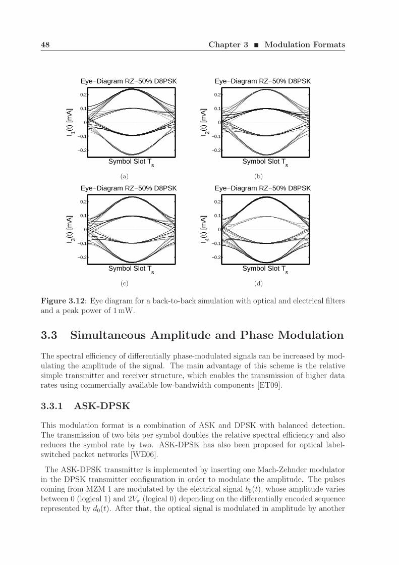
48 Chapter 3 ¥ Modulation Formats
−0.2
−0.1
0
0.1
0.2
Symbol Slot Ts
I 1(t)
[mA
]
Eye−Diagram RZ−50% D8PSK
(a)
−0.2
−0.1
0
0.1
0.2
Symbol Slot Ts
I 2(t)
[mA
]
Eye−Diagram RZ−50% D8PSK
(b)
−0.2
−0.1
0
0.1
0.2
Symbol Slot Ts
I 3(t)
[mA
]
Eye−Diagram RZ−50% D8PSK
(c)
−0.2
−0.1
0
0.1
0.2
Symbol Slot Ts
I 4(t)
[mA
]
Eye−Diagram RZ−50% D8PSK
(d)
Figure 3.12: Eye diagram for a back-to-back simulation with optical and electrical filtersand a peak power of 1 mW.
3.3 Simultaneous Amplitude and Phase Modulation
The spectral efficiency of differentially phase-modulated signals can be increased by mod-ulating the amplitude of the signal. The main advantage of this scheme is the relativesimple transmitter and receiver structure, which enables the transmission of higher datarates using commercially available low-bandwidth components [ET09].
3.3.1 ASK-DPSK
This modulation format is a combination of ASK and DPSK with balanced detection.The transmission of two bits per symbol doubles the relative spectral efficiency and alsoreduces the symbol rate by two. ASK-DPSK has also been proposed for optical label-switched packet networks [WE06].
The ASK-DPSK transmitter is implemented by inserting one Mach-Zehnder modulatorin the DPSK transmitter configuration in order to modulate the amplitude. The pulsescoming from MZM 1 are modulated by the electrical signal b0(t), whose amplitude variesbetween 0 (logical 1) and 2Vπ (logical 0) depending on the differentially encoded sequencerepresented by d0(t). After that, the optical signal is modulated in amplitude by another
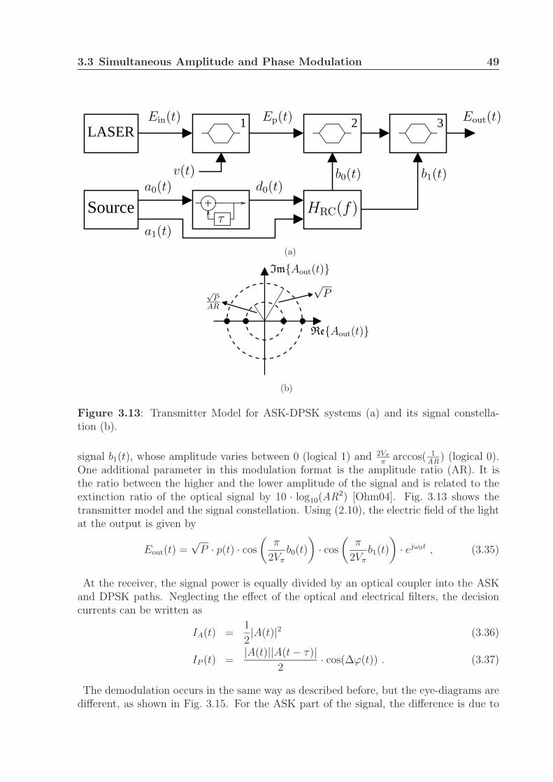
3.3 Simultaneous Amplitude and Phase Modulation 49
LASER
Source
1 2 3
HRC(f)τ
Ein(t) Ep(t)
b0(t)
Eout(t)
a0(t) d0(t)b1(t)
a1(t)
v(t)
(a)
√P
AR
ImAout(t)
ReAout(t)
√P
(b)
Figure 3.13: Transmitter Model for ASK-DPSK systems (a) and its signal constella-tion (b).
signal b1(t), whose amplitude varies between 0 (logical 1) and 2Vπ
πarccos( 1
AR) (logical 0).
One additional parameter in this modulation format is the amplitude ratio (AR). It isthe ratio between the higher and the lower amplitude of the signal and is related to theextinction ratio of the optical signal by 10 · log10(AR2) [Ohm04]. Fig. 3.13 shows thetransmitter model and the signal constellation. Using (2.10), the electric field of the lightat the output is given by
Eout(t) =√
P · p(t) · cos
(π
2Vπ
b0(t)
)· cos
(π
2Vπ
b1(t)
)· ejω0t , (3.35)
At the receiver, the signal power is equally divided by an optical coupler into the ASKand DPSK paths. Neglecting the effect of the optical and electrical filters, the decisioncurrents can be written as
IA(t) =1
2|A(t)|2 (3.36)
IP (t) =|A(t)||A(t − τ)|
2· cos(∆ϕ(t)) . (3.37)
The demodulation occurs in the same way as described before, but the eye-diagrams aredifferent, as shown in Fig. 3.15. For the ASK part of the signal, the difference is due to
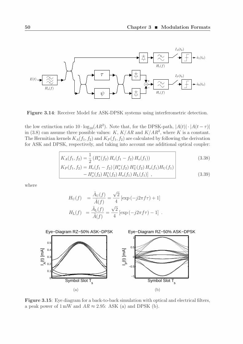
50 Chapter 3 ¥ Modulation Formats
ψ
IP (tk)
a0(tk)
τ
IA(tk)
a1(tk)
He(f)
He(f)Ho(f)
E(t)
Figure 3.14: Receiver Model for ASK-DPSK systems using interferometric detection.
the low extinction ratio 10 · log10(AR2). Note that, for the DPSK-path, |A(t)| · |A(t− τ)|in (3.8) can assume three possible values: K, K/AR and K/AR2, where K is a constant.The Hermitian kernels KA(f1, f2) and KP (f1, f2) are calculated by following the derivationfor ASK and DPSK, respectively, and taking into account one additional optical coupler:
KA(f1, f2) =1
2(H∗
o (f2) He(f1 − f2) Ho(f1))
KP (f1, f2) = He(f1 − f2) [H∗o (f2) H∗
U(f2) Ho(f1)HU(f1)
−H∗o (f2) H∗
L(f2) Ho(f1) HL(f1)] ,
(3.38)
(3.39)
where
HU(f) =AU(f)
A(f)=
√2
4[exp (−j2πfτ) + 1]
HL(f) =AL(f)
A(f)=
√2
4[exp (−j2πfτ) − 1] .
0
0.1
0.2
0.3
0.4
0.5
Symbol Slot Ts
I A(t
) [m
A]
Eye−Diagram RZ−50% ASK−DPSK
(a)
−1
−0.5
0
0.5
1
Symbol Slot Ts
I P(t
) [m
A]
Eye−Diagram RZ−50% ASK−DPSK
(b)
Figure 3.15: Eye diagram for a back-to-back simulation with optical and electrical filters,a peak power of 1 mW and AR ≈ 2.95: ASK (a) and DPSK (b).
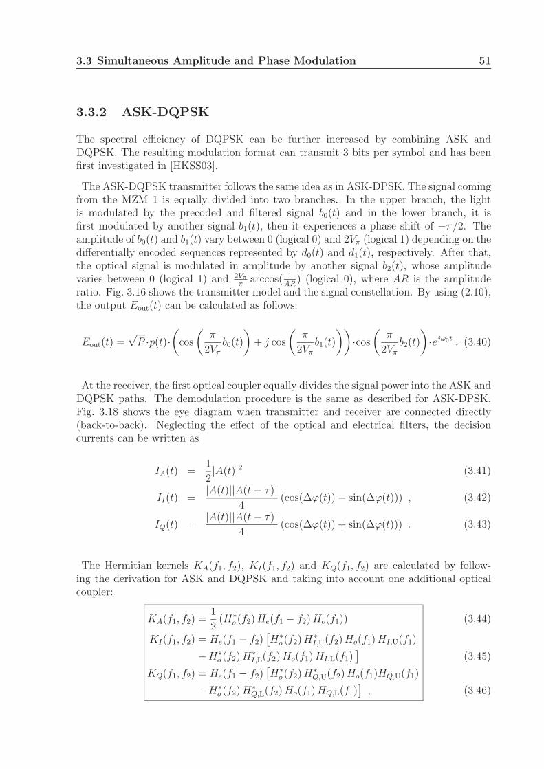
3.3 Simultaneous Amplitude and Phase Modulation 51
3.3.2 ASK-DQPSK
The spectral efficiency of DQPSK can be further increased by combining ASK andDQPSK. The resulting modulation format can transmit 3 bits per symbol and has beenfirst investigated in [HKSS03].
The ASK-DQPSK transmitter follows the same idea as in ASK-DPSK. The signal comingfrom the MZM 1 is equally divided into two branches. In the upper branch, the lightis modulated by the precoded and filtered signal b0(t) and in the lower branch, it isfirst modulated by another signal b1(t), then it experiences a phase shift of −π/2. Theamplitude of b0(t) and b1(t) vary between 0 (logical 0) and 2Vπ (logical 1) depending on thedifferentially encoded sequences represented by d0(t) and d1(t), respectively. After that,the optical signal is modulated in amplitude by another signal b2(t), whose amplitudevaries between 0 (logical 1) and 2Vπ
πarccos( 1
AR) (logical 0), where AR is the amplitude
ratio. Fig. 3.16 shows the transmitter model and the signal constellation. By using (2.10),the output Eout(t) can be calculated as follows:
Eout(t) =√
P ·p(t)·(
cos
(π
2Vπ
b0(t)
)+ j cos
(π
2Vπ
b1(t)
))·cos
(π
2Vπ
b2(t)
)·ejω0t . (3.40)
At the receiver, the first optical coupler equally divides the signal power into the ASK andDQPSK paths. The demodulation procedure is the same as described for ASK-DPSK.Fig. 3.18 shows the eye diagram when transmitter and receiver are connected directly(back-to-back). Neglecting the effect of the optical and electrical filters, the decisioncurrents can be written as
IA(t) =1
2|A(t)|2 (3.41)
II(t) =|A(t)||A(t − τ)|
4(cos(∆ϕ(t)) − sin(∆ϕ(t))) , (3.42)
IQ(t) =|A(t)||A(t − τ)|
4(cos(∆ϕ(t)) + sin(∆ϕ(t))) . (3.43)
The Hermitian kernels KA(f1, f2), KI(f1, f2) and KQ(f1, f2) are calculated by follow-ing the derivation for ASK and DQPSK and taking into account one additional opticalcoupler:
KA(f1, f2) =1
2(H∗
o (f2) He(f1 − f2) Ho(f1))
KI(f1, f2) = He(f1 − f2)[H∗
o (f2) H∗I,U(f2) Ho(f1) HI,U(f1)
−H∗o (f2) H∗
I,L(f2) Ho(f1) HI,L(f1)]
KQ(f1, f2) = He(f1 − f2)[H∗
o (f2) H∗Q,U(f2) Ho(f1)HQ,U(f1)
−H∗o (f2) H∗
Q,L(f2) Ho(f1) HQ,L(f1)]
,
(3.44)
(3.45)
(3.46)
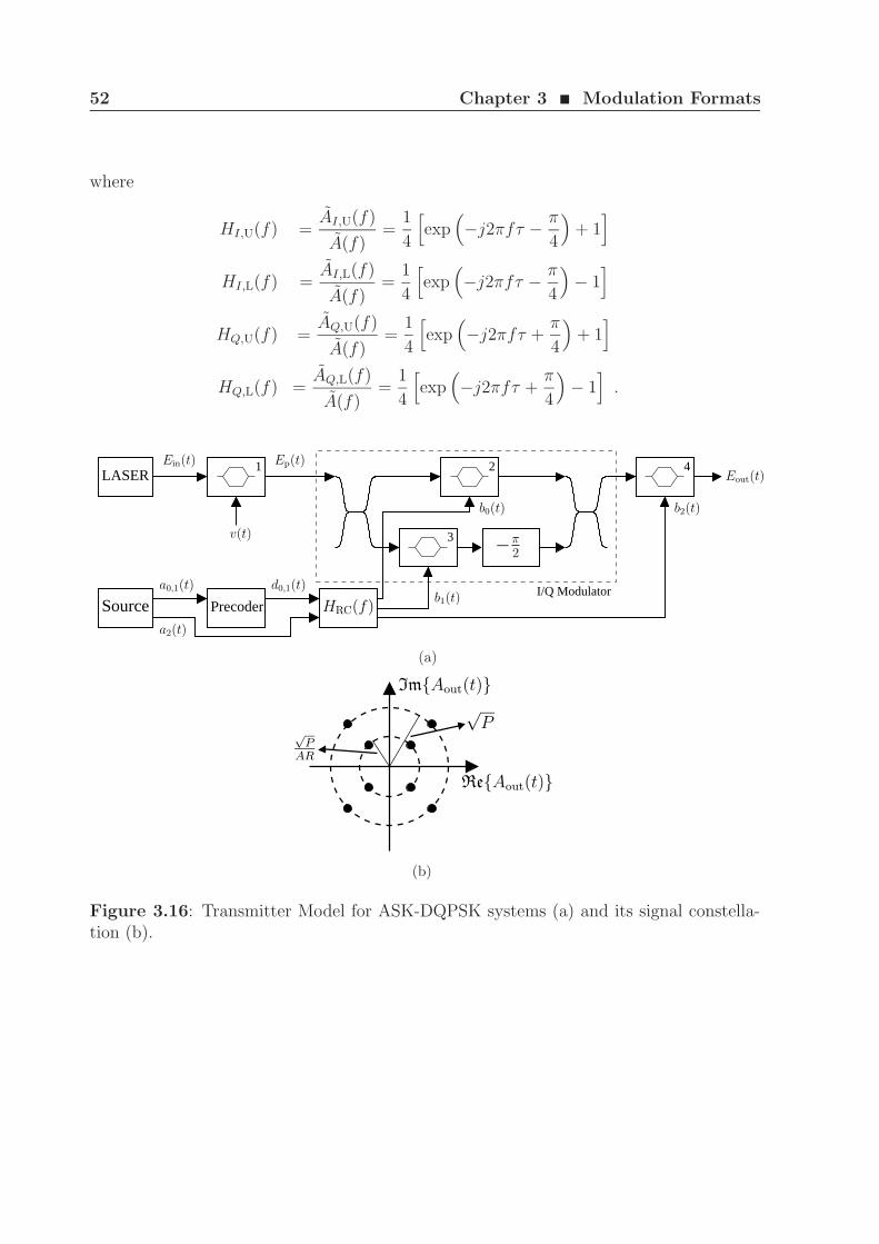
52 Chapter 3 ¥ Modulation Formats
where
HI,U(f) =AI,U(f)
A(f)=
1
4
[exp
(−j2πfτ − π
4
)+ 1
]
HI,L(f) =AI,L(f)
A(f)=
1
4
[exp
(−j2πfτ − π
4
)− 1
]
HQ,U(f) =AQ,U(f)
A(f)=
1
4
[exp
(−j2πfτ +
π
4
)+ 1
]
HQ,L(f) =AQ,L(f)
A(f)=
1
4
[exp
(−j2πfτ +
π
4
)− 1
].
3
2
Source Precoder
LASER1
I/Q Modulator
4
HRC(f)
a0,1(t)
a2(t)
d0,1(t)
Ein(t)
v(t) −π2
b0(t)
Ep(t)Eout(t)
b1(t)
b2(t)
(a)
√P
AR
ImAout(t)
ReAout(t)
√P
(b)
Figure 3.16: Transmitter Model for ASK-DQPSK systems (a) and its signal constella-tion (b).
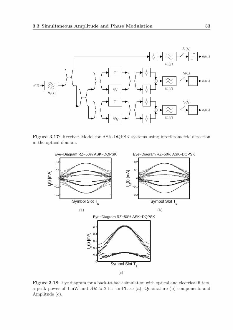
3.3 Simultaneous Amplitude and Phase Modulation 53
ψI
IA(tk)
a2(tk)
IQ(tk)
a1(tk)
τ
II(tk)
a0(tk)
τ
He(f)
He(f)
He(f)
E(t)
Ho(f)
ψQ
Figure 3.17: Receiver Model for ASK-DQPSK systems using interferometric detectionin the optical domain.
−0.2
−0.1
0
0.1
0.2
Symbol Slot Ts
I I(t)
[mA
]
Eye−Diagram RZ−50% ASK−DQPSK
(a)
−0.2
−0.1
0
0.1
0.2
Symbol Slot Ts
I Q(t
) [m
A]
Eye−Diagram RZ−50% ASK−DQPSK
(b)
0
0.1
0.2
0.3
0.4
0.5
Symbol Slot Ts
I A(t
) [m
A]
Eye−Diagram RZ−50% ASK−DQPSK
(c)
Figure 3.18: Eye diagram for a back-to-back simulation with optical and electrical filters,a peak power of 1 mW and AR ≈ 2.11: In-Phase (a), Quadrature (b) components andAmplitude (c).
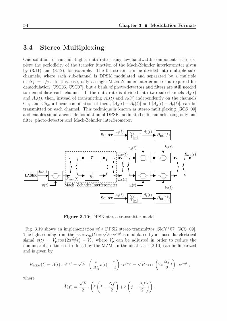
54 Chapter 3 ¥ Modulation Formats
3.4 Stereo Multiplexing
One solution to transmit higher data rates using low-bandwidth components is to ex-plore the periodicity of the transfer function of the Mach-Zehnder interferometer givenby (3.11) and (3.12), for example. The bit stream can be divided into multiple sub-channels, where each sub-channel is DPSK modulated and separated by a multipleof ∆f = 1/τ . In this case, only a single Mach-Zehnder interferometer is required fordemodulation [CSC06, CSC07], but a bank of photo-detectors and filters are still neededto demodulate each channel. If the data rate is divided into two sub-channels Aa(t)and Ab(t), then, instead of transmitting Aa(t) and Ab(t) independently on the channelsCh1 and Ch2, a linear combination of them, [Aa(t) + Ab(t)] and [Aa(t) − Ab(t)], can betransmitted on each channel. This technique is known as stereo multiplexing [GCS+09]and enables simultaneous demodulation of DPSK modulated sub-channels using only onefilter, photo-detector and Mach-Zehnder interferometer.
Source
Source
LASER
Mach−Zehnder Interferometer
τHRC(f)
d1(t)a1(t)
τ
d0(t)HRC(f)
a0(t)
EU(t)τ
ψEin(t)
v(t)
EL(t)
vb(t)
va(t)
Eout(t)
b0(t)
b1(t)
EMZM(t)
Figure 3.19: DPSK stereo transmitter model.
Fig. 3.19 shows an implementation of a DPSK stereo transmitter [SMY+07, GCS+09].The light coming from the laser Ein(t) =
√P · ejω0t is modulated by a sinusoidal electrical
signal v(t) = Vp cos(2π∆f
2t)− Vπ, where Vp can be adjusted in order to reduce the
nonlinear distortions introduced by the MZM. In the ideal case, (2.10) can be linearizedand is given by
EMZM(t) = A(t) · ejω0t =√
P ·(
π
2Vπ
v(t) +π
2
)· ejω0t =
√P · cos
(2π
∆f
2t
)· ejω0t ,
where
A(f) =
√P
2·(
δ
(f − ∆f
2
)+ δ
(f +
∆f
2
)),

3.4 Stereo Multiplexing 55
Vp = 2Vπ
πand δ(·) is the Dirac delta function. Note that two coherent sub-carriers were
generated in this process. By setting the phase ψ in (3.11) and (3.12) to ψ = −2π∆f
2τ −
ω0τ , the transfer functions of the upper HU(f) and lower HL(f) branches are given by
HU(f) =AU(f)
A(f)= j ejψ · exp
(−j2π
(f − ∆f
2
)τ)
+ 1
2(3.47)
HL(f) =AU(f)
A(f)= −ejψ · exp
(−j2π
(f − ∆f
2
)τ)− 1
2, (3.48)
where τ = 12∆f
, EU(t) = AU(t) · ejω0t and EL(t) = AL(t) · ejω0t. Assuming that the MZM
is perfectly linear, then EU(t), EL(t) and Eout(t) are given by
EU(t) =
√P
2· j ejψ · ej(ω0+∆ω
2 )t , EL(t) =
√P
2· ejψ · ej(ω0−∆ω
2 )t (3.49)
Eout(t) =1√2
[Aa(t) − Ab(t)
2· ej ∆ω
2t +
Aa(t) + Ab(t)
2· e−j ∆ω
2t
]· j ejψ · ejω0t ,(3.50)
where ∆ω = 2π∆f , Aa(t) =√
P · pa(t) · cos(
π2Vπ
b0(t)), Ab(t) =
√P · pb(t) · cos
(π
2Vπb1(t)
)
and pa,b(t) = cos(
π2Vπ
va,b(t)). The factor j ejψ has no influence on the modulation and
will be dropped.
Ho(f)
E(t)
τ
ψ He(f)
He(f)2 cos(2π∆ft)
Ia(t)
Ib(t)
I(t)
Figure 3.20: DPSK stereo receiver model.
Fig. 3.20 shows the structure of a stereo multiplexed DPSK receiver. Neglecting theeffect of the optical filter Ho(f), the signal I(t) is given by
I(t) = ReE(t) · E∗(t − τ) · ejψ
(3.51)
=1
8Re
2AaA
∗a,τ + 2AbA
∗b,τ +
(AaA
∗a,τ + AaA
∗b,τ − AbA
∗a,τ − AbA
∗b,τ
)ej2π∆ft+
(AaA
∗a,τ − AaA
∗b,τ + AbA
∗a,τ − AbA
∗b,τ
)e−j2π∆ft
(3.52)
where ψ = −ω0τ , Aa = Aa(t), Ab = Ab(t), Aa,τ = Aa(t − τ) and Ab,τ = Ab(t − τ). Notethat the information in the sub-channels a and b can be recovered by mixing and filteringI(t), as shown in Fig. 3.20, or by sampling I(t) at t = k
2∆f, k ∈ 1, 2, 3, . . ..
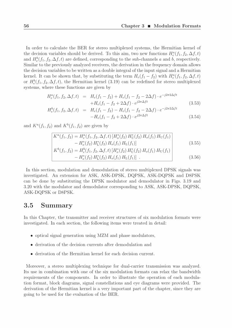
56 Chapter 3 ¥ Modulation Formats
In order to calculate the BER for stereo multiplexed systems, the Hermitian kernel ofthe decision variables should be derived. To this aim, two new functions Ha
e (f1, f2, ∆f, t)and Hb
e(f1, f2, ∆f, t) are defined, corresponding to the sub-channels a and b, respectively.Similar to the previously analyzed receivers, the derivation in the frequency domain allowsthe decision variables to be written as a double integral of the input signal and a Hermitiankernel. It can be shown that, by substituting the term He(f1 − f2) with Ha
e (f1, f2, ∆f, t)or Hb
e(f1, f2, ∆f, t), the Hermitian kernel (3.19) can be redefined for stereo multiplexedsystems, where these functions are given by
Hae (f1, f2, ∆f, t) = He(f1 − f2) + He(f1 − f2 − 2∆f) · e−j2π2∆ft
+He(f1 − f2 + 2∆f) · ej2π∆ft (3.53)
Hbe(f1, f2, ∆f, t) = He(f1 − f2) − He(f1 − f2 − 2∆f) · e−j2π2∆ft
−He(f1 − f2 + 2∆f) · ej2π∆ft (3.54)
and Ka(f1, f2) and Kb(f1, f2) are given by
Ka(f1, f2) = Hae (f1, f2, ∆f, t) [H∗
o (f2) H∗U(f2) Ho(f1) HU(f1)
−H∗o (f2) H∗
L(f2) Ho(f1) HL(f1)]
Kb(f1, f2) = Hbe(f1, f2, ∆f, t) [H∗
o (f2) H∗U(f2) Ho(f1) HU(f1)
−H∗o (f2) H∗
L(f2) Ho(f1) HL(f1)] .
(3.55)
(3.56)
In this section, modulation and demodulation of stereo multiplexed DPSK signals wasinvestigated. An extension for ASK, ASK-DPSK, DQPSK, ASK-DQPSK and D8PSKcan be done by substituting the DPSK modulator and demodulator in Figs. 3.19 and3.20 with the modulator and demodulator corresponding to ASK, ASK-DPSK, DQPSK,ASK-DQPSK or D8PSK.
3.5 Summary
In this Chapter, the transmitter and receiver structures of six modulation formats wereinvestigated. In each section, the following items were treated in detail:
• optical signal generation using MZM and phase modulators,
• derivation of the decision currents after demodulation and
• derivation of the Hermitian kernel for each decision current.
Moreover, a stereo multiplexing technique for dual-carrier transmission was analyzed.Its use in combination with one of the six modulation formats can relax the bandwidthrequirements of the components. In order to illustrate the operation of each modula-tion format, block diagrams, signal constellations and eye diagrams were provided. Thederivation of the Hermitian kernel is a very important part of the chapter, since they aregoing to be used for the evaluation of the BER.
4Evaluation of the Bit-error Rate
In long-haul fiber-optic communication systems, the bit-error rate (BER) is basicallydetermined by PMD, fiber dispersion, fiber nonlinearity and the accumulated noise gen-erated by the optical amplifiers through spontaneous emission. The accurate computationof the BER is the most complex part in the receiver modeling. Conventional methodsthat approximate the probability density function (PDF) at the receiver to a Gaussiandistribution or use the standard Q-factor analysis do not work in phase-modulated sys-tems, even if the received noise is white and Gaussian [BP04, GW05]. Assuming that thereceived optical noise is AWGN, the BER can be exactly evaluated using several methodsbased on the principle of Karhunen-Loeve series expansion [KS47, LS94, For00, GW05].However, when the light propagates inside the fiber, the ASE noise interacts with thesignal through the Kerr effect, which induces nonlinear signal phase fluctuations andchanges the received optical noise statistics. This is known in the literature as nonlinearphase noise [GM90]. For instance, it was shown experimentally that the advantages ofusing DPSK together with balanced detection can vanish as nonlinear phase noise be-comes dominant over other impairments [KG03]. Therefore, the performance evaluationof advanced modulation formats should include the interaction between signal and noisein order to correctly assess the BER, as well as system margins and reach.
The most straightforward method to evaluate the BER is the standard Monte Carlosimulation. It includes the interaction between signal and noise and is often used as ref-erence for other simulation techniques. For BER’s smaller than 10−6, the multi-canonicalMonte Carlo method [HM03] is more efficient. However, if the BER has to be computedseveral times, the overall computational effort of both Monte Carlo methods is so largethat it becomes unpractical to apply these methods for optimizing systems including, forexample, nonlinear phase noise.
58 Chapter 4 ¥ Evaluation of the Bit-error Rate
The simulation time can be drastically reduced by deriving simplified models or closed-form expressions for the BER. For example, if the distribution of the differential phasenoise in DPSK systems is approximated as Gaussian, then a differential phase Q-method [WLX03] can be used to qualitatively estimate the BER in the presence ofnonlinear phase noise. In absence of dispersion, the statistics of the noise at the re-ceiver and, therefore, the BER can be exactly calculated using an optical matched fil-ter [Mec94, Ho05, DPL08]. A simplified method developed by Ho [Ho05], was verifiedexperimentally [HHC+05], where a good agreement between simulation and experimentwas achieved. However, in the presence of dispersion, the method overestimates the impactof nonlinear phase noise. Using a perturbational analysis, Ho and Wang also investigatedthe effect of dispersion on nonlinear phase noise [HW06], but they used second-orderstatistics as a measure of the performance instead of the BER.
Fiber dispersion and nonlinear phase noise can be adequately taken into account by us-ing techniques based on the linearization of the nonlinear Schrodinger equation (NLSE).Comparing to the standard and multi-canonical Monte Carlo methods, the computationaleffort can be significantly reduced at a cost of neglecting the nonlinear noise-noise inter-action and intra-channel effects. The main idea of a linearization procedure is to separatethe analysis of the signal and noise, i.e., the split-step Fourier method [Agr06] accountsfor nonlinear signal-signal distortion and the interaction between signal and noise is eval-uated by solving the NLSE, where the signal is a non-modulated carrier and the noiseacts as a perturbation of the general solution. In this case, the quadratic nonlinearity ofthe photodetector is kept and the linearization is only performed on the nonlinear termof the NLSE. A comprehensive review of these techniques can be found in Demir’s pa-per [Dem07]. This approach has been extensively used to simplify the analysis of theNLSE in the presence of noise. The main difference between several methods based onlinearization [HORT97, SOB06, Agr05b, CWI98, CWI99, HGMK02, HMKG03] is the useof a real/imaginary or amplitude/phase representation of the ASE noise. For example,Holzlohner et al. [HGMK02] used a generalization of [Mar90] and a real/imaginary rep-resentation of the noise to derive a covariance matrix method. In this case, timing andphase jitter were separated in order to accurately evaluate eye diagrams and BER’s forcommunication systems based on solitons. However, the method relies on the correctevaluation of a covariance matrix, whose computational cost equals that of a Monte Carlosimulation [HMKG03]. Moreover, the separation of phase and timing jitter may not beapplicable to phase-modulated systems.
In this chapter, five methods for evaluating the BER are derived and validated. First,the probability of error using optical matched filters is evaluated analytically and takenas a reference. Following, a linearization technique of the NLSE is used to derive a systemtransmission matrix W(f). Then, the standard Karhunen-Loeve method is derived andthe matrix W(f) is applied together with Karhunen-Loeve method to evaluate the BERin the presence of nonlinear phase noise. In order to validate the simulation method, anexperiment was performed, where the effect of dispersion on nonlinear phase noise wasinvestigated. Finally, the standard and multi-canonical Monte Carlo methods are derivedand compared to the Karhunen-Loeve methods.
4.1 Error Probability using Optical Matched Filters 59
4.1 Error Probability using Optical Matched Filters
The BER is defined as the number of received bits in error divided by the total numberof transmitted bits during a time interval. Considering a long information sequence a0,the bit-error probability Pb is the expected value of the BER. In this section, the bit-errorprobability is derived for the modulation formats presented in Chapter 3.
Ideally, the electrical field of an OOK modulated optical signal is given by
E(t) = A(t) · ejω0t =√
κp ·∑
k
p(t − kTs) · ak0 · ejω0t , (4.1)
where κp is a dimensionless constant which guarantees that max (p(t)) = 1√
W, ak0 ∈
0, 1 and p(t) is the pulse format in units of√
W. Different pulse formats can befound in Table 3.1. In optically pre-amplified receivers, the best system performance isachieved with an optical matched filter and no post-detection electrical filtering [Hen89,PSPW02]. In this case, signal distortion introduced by filtering and noise are balanced.The impulse response and transfer function of an optical matched filter for these signalsis given by [Pro95]
hMF(t) = κf · p(Ts − t) , (4.2)
HMF(f) = κf · P ∗(f) · exp (−j2πfTs) . (4.3)
where κf is a normalization constant in 1/(√
Ws). Considering the receiver structure inFig. 3.2, I(t) can be calculated as
I(t) = R · |A(t) ∗ hMF(t)|2
= R ·∣∣∣∣∣
∫ ∞
−∞
√κp ·
∑
k
p(t − τ − kTs) · ak0 · κf · p(Ts − τ) dτ
∣∣∣∣∣
2
, (4.4)
where R =1 A/W is the photodiode responsivity, ∗ is the convolution operator, Ho(f) =HMF(f) and He(f) = 1. The current I(t) is maximum at the sampling point t = tk =(k + 1) · Ts, which results in
I(tk) =
∣∣∣∣∫ ∞
−∞
√κp · p(Ts − τ) · ak
0 · κf · p(Ts − τ) dτ
∣∣∣∣2
=∣∣√κp · ak
0 · κf · εp
∣∣2 , (4.5)
where εp =∫ ∞−∞ |P (f)|2df is the energy of the pulse and P (f) the Fourier transform of
p(t). The power spectral density (PSD) of the ASE noise after the optical matched filteron each polarization is given by ΦMF(f) = |HMF(f)|2 ·ΦASE. Including ASE noise on bothpolarizations, the decision variable I(tk) can be written as
I(tk) =∣∣√κp · ak
0 · εp + nMFx (tk)
∣∣2 +∣∣nMF
y (tk)∣∣2 , (4.6)
where nMFx (t) and nMF
y (t) are ASE noise after the matched filter and nMFx (tk) and nMF
y (tk)are complex Gaussian random variables with variance 2σ2
MF = ΦASE · κ2f · εp. Fig 4.1
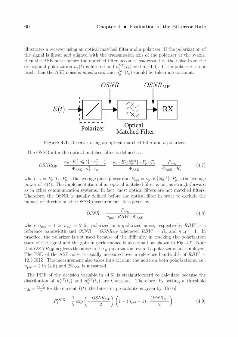
60 Chapter 4 ¥ Evaluation of the Bit-error Rate
illustrates a receiver using an optical matched filter and a polarizer. If the polarization ofthe signal is linear and aligned with the transmission axis of the polarizer at the x-axis,then the ASE noise before the matched filter becomes polarized, i.e. the noise from theorthogonal polarization ny(t) is filtered and nMF
y (tk) = 0 in (4.6). If the polarizer is notused, then the ASE noise is unpolarized and nMF
y (tk) should be taken into account.
Polarizer
RX
Optical Matched Filter
E(t)
OSNR OSNRMF
Figure 4.1: Receiver using an optical matched filter and a polarizer.
The OSNR after the optical matched filter is defined as
OSNRMF =κp · E|ak
0|2 · κ2f · ε2
p
ΦASE · κ2f · εp
=κp · E|ak
0|2 · Pp · Ts
ΦASE
=Pavg
ΦASE · Rs
(4.7)
where εp = Pp ·Ts, Pp is the average pulse power and Pavg = κp ·E|ak0|2·Pp is the average
power of A(t). The implementation of an optical matched filter is not as straightforwardas in other communication systems. In fact, most optical filters are not matched filters.Therefore, the OSNR is usually defined before the optical filter in order to exclude theimpact of filtering on the OSNR measurement. It is given by
OSNR =Pavg
npol · RBW · ΦASE
(4.8)
where npol = 1 or npol = 2 for polarized or unpolarized noise, respectively, RBW is areference bandwidth and OSNR = OSNRMF whenever RBW = Rs and npol = 1. Inpractice, the polarizer is not used because of the difficulty in tracking the polarizationstate of the signal and the gain in performance is also small, as shown in Fig. 4.9. Notethat OSNRMF neglects the noise in the y-polarization, even if a polarizer is not employed.The PSD of the ASE noise is usually measured over a reference bandwidth of RBW =12.5 GHZ. The measurement also takes into account the noise on both polarizations, i.e.,npol = 2 in (4.8) and 2ΦASE is measured.
The PDF of the decision variable in (4.6) is straightforward to calculate because thedistribution of nMF
x (tk) and nMFy (tk) are Gaussian. Therefore, by setting a threshold
γth =κp·ε2
p
4for the current I(t), the bit-error probability is given by [Ho05]
POOKb =
1
2exp
(−OSNRMF
2
) (1 + (npol − 1) · OSNRMF
2
), (4.9)
4.2 Linearization of the Nonlinear Schrodinger Equation 61
Similarly, the bit-error probability can be calculated for other modulation formats [Ho05,HL06, NSY06], as shown in Appendix A. The bit-error probabilities POOK
b , PDPSKb ,
PASK−DPSKb , PDQPSK
b , PASK−DQSPKb and PD8PSK
b set the limit for the best performance andare usually refereed as the quantum limit for a certain modulation format. Throughoutthis thesis, they are going to be used as the first guess of the system performance.
4.2 Linearization of the Nonlinear Schrodinger Equa-
tion
Noise enhancement due to fiber nonlinearities can be found in the literature under severalnames [HORT97, SOB06, Agr05b]. Modulation Instability, Parametric Gain, four-wave-mixing (FWM) between signal and noise are few examples. Despite different names, theyall rely on the same mathematical formalism to evaluate the impact of amplified ASE noiseon the system performance. In this section, a linearization technique of the NLSE (2.66)is used in order to evaluate the noise enhancement due to fiber nonlinearities and also todefine a system transmission matrix W(f), which accounts for the nonlinear interactionbetween signal and noise.
Consider a slowly varying complex envelope at the input of an optical fiber A′(z = 0, t) =s(z = 0, t)+a(z = 0, t), where s(z = 0, t) is the signal with peak power P0 and a(z = 0, t)is the ASE of a single optical amplifier in one polarization. The scalar NLSE describesthe propagation of this signal and noise inside the fiber and is given by
∂A′(z, t)
∂z− j
2β2
∂2A′(z, t)
∂t2− 1
6β3
∂3A′(z, t)
∂t3= −jγavg|A′(z, t)|2A′(z, t) · e−αz , (4.10)
where A′(z, t) is related to A(z, t) from (2.66) by A(z, t) = A′(z, t) · e−α2
z. If the signals(z, t) is much stronger than the noise a(z, t), then the NLSE can be linearized by ne-glecting the noise-noise beat term arising from the fiber nonlinearity, i.e. terms involvingan(z, t), where n > 1, are not taken into account. In the following, a single fiber of lengthL is analyzed, then the result is extended for a multi-span system.
4.2.1 Single fiber
Considering the signal s(z = 0, t) as unmodulated with power P0 and neglecting the noisea(z = 0, t), i.e. A′(z, t) becomes A′(z), the NLSE (4.10) reduces to
∂A′(z)
∂z= −jγavgP0A
′(z) · e−αz
A′(z) =√
P0 · e−jφ(z) , (4.11)
where φ(z) = γavgP0
∫ z
0e−αz′dz′. If the noise a(z, t) is added to the solution as a pertur-
bation, we have
A′(z, t) = (√
P0 + a(z, t)) · e−jφ(z) . (4.12)
62 Chapter 4 ¥ Evaluation of the Bit-error Rate
Using (4.12) and assuming that |a(z, t)|2 ≪ P0, the following terms can be derived:
∂A′(z, t)
∂z=
[∂a(z, t)
∂z+ (
√P0 + a(z, t)) · (−jγP0)e
−αz
]· e−jφ(z) , (4.13)
∂2A′(z, t)
∂t2=
∂2a(z, t)
∂t2· e−jφ(z) , (4.14)
∂3A′(z, t)
∂t3=
∂3a(z, t)
∂t3· e−jφ(z) , (4.15)
|A′(z, t)|2A′(z, t) = (√
P0P0 + 2P0a(z, t) + P0a∗(z, t)) · e−jφ(z) , (4.16)
Substituting these terms in (4.10), the following equation and its complex conjugate areobtained
∂a(z, t)
∂z=
j
2β2
∂2a(z, t)
∂t2+
1
6β3
∂3a(z, t)
∂t3− jγavgP0e
−αz(a(z, t) + a∗(z, t)) (4.17)
∂a∗(z, t)
∂z= −j
2β2
∂2a∗(z, t)
∂t2+
1
6β3
∂3a∗(z, t)
∂t3+ jγavgP0e
−αz(a(z, t) + a∗(z, t)) . (4.18)
In time domain, the noise is given by a(z, t) = ap(z, t) + jaq(z, t), where ap(z, t) andaq(z, t) are the in-phase and quadrature components of the noise, respectively, and they arealso real functions. The power spectral density of the ASE noise in one polarization is givenby (2.12) and the power of the noise before optical filtering is given by PASE = ΦASE·RBW ,where RBW is a reference bandwidth or the simulation bandwidth, if the noise is goingto be added to the signal. According to the Wiener-Kinchine theorem, ΦASE is calculatedby taking the Fourier transform of the autocorrelation function of a(z, t). Alternatively,ΦASE may be calculated from a(z, ω). In order to take the Fourier transform of a(z, t), itmust be square integrable, i.e.
∫ ∞
−∞|a(z, t)|2dt < ∞ . (4.19)
This condition can never be satisfied by any sample function of a(z, t). In order to usethe Fourier transform, a truncated interval of a(z, t), for example −τ < t < τ , should beconsidered. Thus, the Fourier transform of a(z, t) over this interval is given by
a(z, ω, τ) =
∫ τ
−τ
a(z, t) exp(−jωt)dt (4.20)
In this case, the power spectral density of a(z, t) can be calculated using
ΦASE = limτ→∞
1
τE
|a(z, ω, τ)|2
, (4.21)
which is the same as taking the Fourier transform of the autocorrelation function ofa(z, t). From now on, the term τ in a(z, ω, τ) is going to be omitted and when the Fouriertransform is applied on a random process, it will be considered over a time window.
4.2 Linearization of the Nonlinear Schrodinger Equation 63
Using (4.17) and (4.18) and 2ap(z, t) = a(z, t) + a∗(z, t), the evolution of the in-phaseand quadrature components can be separated and are given in time domain by
∂ap(z, t)
∂z= −β2
2
∂2aq(z, t)
∂t2+
1
6β3
∂3ap(z, t)
∂t3(4.22)
∂aq(z, t)
∂z=
β2
2
∂2ap(z, t)
∂t2+
1
6β3
∂3aq(z, t)
∂t3− 2jγavgP0e
−αzap(z, t) , (4.23)
in frequency domain by
∂ap(z, ω)
∂z=
β2ω2
2aq(z, ω) − j
6β3ω
3ap(z, ω) (4.24)
∂aq(z, ω)
∂z= −β2ω
2
2ap(z, ω) − j
6β3ω
3aq(z, ω) − 2jγavgP0e−αzap(z, ω) , (4.25)
and in a matrix form by
∂
∂z
[ap(z, ω)aq(z, ω)
]=
[−jκ ρ
− (ρ + 2γavgP0e−αz) −jκ
] [ap(z, ω)aq(z, ω)
](4.26)
where κ = β3ω3
6and ρ = β2ω2
2. The solution of this equation is in the form
aout = M · ain , (4.27)
where a = [ap(z, ω) aq(z, ω)]T and the transmission matrix M is given by
M = exp
∫ L
0
[−jκ ρ
−(ρ + 2γavgP0e
−αz′)
−jκ
]dz′
. (4.28)
In the absence of loss, M is given by
M = f(A) = eA , (4.29)
where
A =
[−jκL ρL
−ρL − 2γavgP0L −jκL
]. (4.30)
The characteristic polynomial ∆(λ) of A is given by
∆(λ) = det |λ · I − A| =
∣∣∣∣λ + jκL −ρL
ρL + 2γavgP0L λ + jκL
∣∣∣∣ ,
= λ2 + 2jλκL − κ2L2 + ρ2L2 + 2ργavgP0L2 ,
= (λ − λ1) · (λ − λ2) , (4.31)
where I is the identity matrix, λ1 = −jκL + jδL, λ2 = −jκL − jδL and δ =√ρ(ρ + 2γavgP0). The function f(λ) may be expanded as
f(λ) = eλ =∞∑
k=0
1
k!λk (4.32)
64 Chapter 4 ¥ Evaluation of the Bit-error Rate
and, using the characteristic polynomial, f(λ) may also be written as
f(λ) = ∆(λ) h(λ) + g(λ) , (4.33)
where g(λ) = α0 +α1λ is a polynomial of degree 1 or 0. Note that for λ = λ1 and λ = λ2,f(λ1) = g(λ1) and f(λ2) = g(λ2), respectively. Therefore, α0 and α1 can be calculated as
f(λ1) = g(λ1) ⇒ eλ1 = α0 + α1λ1 (4.34)
f(λ2) = g(λ2) ⇒ eλ2 = α0 + α1λ2 (4.35)
α0 = exp(−jκL)
(jκ
δsin(δL) + cos(δL)
)(4.36)
α1 =exp(−jκL)
δLsin(δL) . (4.37)
The Cayley-Hamilton theorem [Str06] states that every matrix satisfies its own charac-teristic equation, that is
∆(A) = 0 . (4.38)
where 0 is the zero matrix. Consequently, M is given by
M = f(A) = ∆(A) h(A) + g(A) = α0 + α1 · A ,
= exp(−jκL)
[cos(δL) ρL · sinc(δL)
−L (ρ + 2γavgP0) · sinc(δL) cos(δL)
]. (4.39)
where sinc(δL) = sin(δL)δL
. Note that δ is imaginary when β2 < 0 and |β2ω2
2| < 2γavgP0,
then sin → sinh and cos → cosh.
The transmission matrix with α 6= 0 can be obtained by dividing the fiber into manyshort pieces of length dz. The total transmission matrix is given by the ordered product ofthe transmission matrices for each segment of the fiber [HORT97, GMW03]. If dz ≪ α−1
and dz = LNsec
being Nsec ∈ N , a mean-field approximation can be applied in each section
M = exp(−jκL) · limdz→0
Nsec∏
i=1
[cos(δidz) ρdz · sinc(δidz)
−dz (ρ + 2γidz
P0) · sinc(δidz) cos(δidz)
], (4.40)
=
[M11(ω) M12(ω)M21(ω) M22(ω)
],
where δi and γidz
for each segment are given by
δi =√
ρ2 + 2ργidz
P0 , (4.41)
γidz
=1 − exp(−αdz)
αdz· γavg · e−α(i−1)dz . (4.42)
Note that this solution does not take into account the attenuation of the signal and noiseduring the propagation. The attenuation was included in the calculation as a factor which
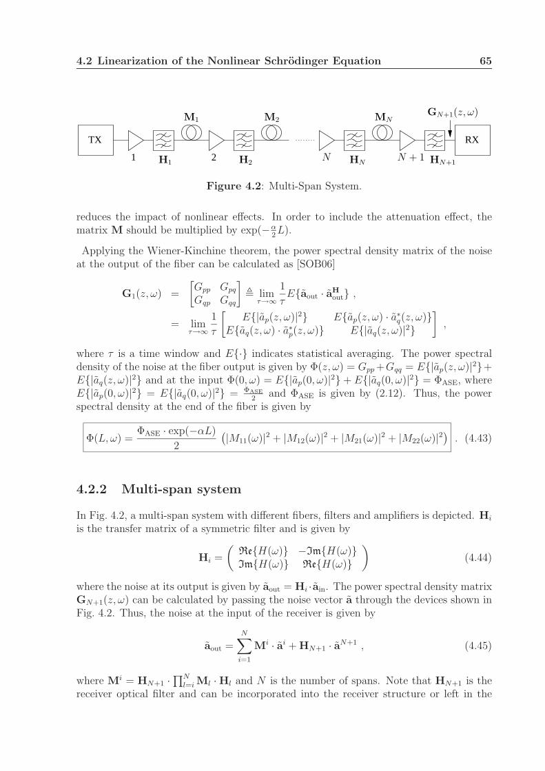
4.2 Linearization of the Nonlinear Schrodinger Equation 65
RXTX
21
GN+1(z, ω)
H1 H2
M2M1
N HNN + 1 HN+1
MN
Figure 4.2: Multi-Span System.
reduces the impact of nonlinear effects. In order to include the attenuation effect, thematrix M should be multiplied by exp(−α
2L).
Applying the Wiener-Kinchine theorem, the power spectral density matrix of the noiseat the output of the fiber can be calculated as [SOB06]
G1(z, ω) =
[Gpp Gpq
Gqp Gqq
], lim
τ→∞
1
τEaout · aH
out ,
= limτ→∞
1
τ
[E|ap(z, ω)|2 Eap(z, ω) · a∗
q(z, ω)Eaq(z, ω) · a∗
p(z, ω) E|aq(z, ω)|2
],
where τ is a time window and E· indicates statistical averaging. The power spectraldensity of the noise at the fiber output is given by Φ(z, ω) = Gpp +Gqq = E|ap(z, ω)|2+E|aq(z, ω)|2 and at the input Φ(0, ω) = E|ap(0, ω)|2 + E|aq(0, ω)|2 = ΦASE, whereE|ap(0, ω)|2 = E|aq(0, ω)|2 = ΦASE
2and ΦASE is given by (2.12). Thus, the power
spectral density at the end of the fiber is given by
Φ(L, ω) =ΦASE · exp(−αL)
2
(|M11(ω)|2 + |M12(ω)|2 + |M21(ω)|2 + |M22(ω)|2
). (4.43)
4.2.2 Multi-span system
In Fig. 4.2, a multi-span system with different fibers, filters and amplifiers is depicted. Hi
is the transfer matrix of a symmetric filter and is given by
Hi =
(ReH(ω) −ImH(ω)ImH(ω) ReH(ω)
)(4.44)
where the noise at its output is given by aout = Hi · ain. The power spectral density matrixGN+1(z, ω) can be calculated by passing the noise vector a through the devices shown inFig. 4.2. Thus, the noise at the input of the receiver is given by
aout =N∑
i=1
Mi · ai + HN+1 · aN+1 , (4.45)
where Mi = HN+1 ·∏N
l=i Ml · Hl and N is the number of spans. Note that HN+1 is thereceiver optical filter and can be incorporated into the receiver structure or left in the
66 Chapter 4 ¥ Evaluation of the Bit-error Rate
link. Therefore, the power spectral density of the noise can be calculated as follows:
GN+1(z, ω) =
[Gpp Gpq
Gqp Gqq
], lim
τ→∞
1
τEaout · aH
out
= E
(N∑
i=1
Mi · ai + HN+1 · aN+1
)·(
N∑
i=1
Mi · ai + HN+1 · aN+1
)H
=N∑
i=1
Mi · Eai(ai)H · (Mi)H + HN+1 · EaN+1(aN+1)H · HH
N+1
=N∑
i=1
Mi(Mi)H · ΦiASE
2+ HN+1 · HH
N+1 ·ΦN+1
ASE
2
=ΦN+1
ASE
2
(N∑
i=1
Mi(Mi)HΦi
ASE
ΦN+1ASE
+ HN+1HH
N+1
), (4.46)
where ΦiASE is the power spectral density of the ASE noise generated by the i-th amplifier.
Using (4.40), Gpp, Gpq, Gqp and Gqq can be evaluated in order to calculate the Φ(z, ω) atthe receiver input:
Gpp =ΦN+1
ASE
2
(N∑
i=1
(|M i
11(ω)|2 + |M i12(ω)|2
)· Φi
ASE
ΦN+1ASE
+ |HN+1(ω)|2)
(4.47)
Gpq =ΦN+1
ASE
2
(N∑
i=1
(M i11(ω)[M i
21(ω)]∗ + M i12(ω)[M i
22(ω)]∗) · ΦiASE
ΦN+1ASE
)(4.48)
Gqp =ΦN+1
ASE
2
(N∑
i=1
(M i21(ω)[M i
11(ω)]∗ + M i22(ω)[M i
12(ω)]∗) · ΦiASE
ΦN+1ASE
)(4.49)
Gqq =ΦN+1
ASE
2
(N∑
i=1
(|M i
21(ω)|2 + |M i22(ω)|2
)· Φi
ASE
ΦN+1ASE
+ |HN+1(ω)|2)
(4.50)
Note that each term in the sum (4.46) has a product of the matrices Mi. In order to goover the sum only one time, it is necessary to calculate the system transmission matrixbackwards, i.e., the sum should be calculated from i = N to 1. Several properties of theinteraction between signal and noise can be evaluated using the power spectral densitymatrix GN+1(z, ω), as reported in [SBO07]. It is important to note that GN+1(z, ω) is a
positive semidefinite matrix and, therefore, it can be written as GN+1(z, ω) =ΦN+1
ASE
2· (W ·
WH), where [Str06, SOB06]
W =
√2
ΦN+1ASE
√Gpp 0(
G∗pq√Gpp
) √∣∣∣Gqq − |Gpq |2Gpp
∣∣∣
(4.51)
4.2 Linearization of the Nonlinear Schrodinger Equation 67
and the statistics of the received noise is equivalent to an AWGN noise with power spectraldensity ΦN+1
ASE · I filtered by W. Therefore, the noise at the receiver input is given by
aout = W · aN+1 =
(W11(ω) W12(ω)
W21(ω) W22(ω)
)· aN+1 . (4.52)
The noise statistics of every ai was normalized by aN+1 and is included in W. Note thatin a(z, ω) = ap(z, ω)+ jaq(z, ω), ap(z, ω) and aq(z, ω) may be complex functions. In orderto deal with system functions in the frequency domain, it is more convenient to definea noise vector n(z, ω) = [nre(z, ω) nim(z, ω)]T containing the real and imaginary parts ofa(z, ω):
nre(z, ω) = Rea(z, ω) =a(z, ω) + a∗(z, ω)
2(4.53)
nim(z, ω) = Ima(z, ω) =a(z, ω) − a∗(z, ω)
2j(4.54)
By defining a discrete symmetric frequency vector in equivalent baseband f =[f−M f−M+1 . . . 0 . . . fM−1 fM ]T and using the relation ω = 2πf , the vector nout(z, f)can be written as a (4M +2)×1 column vector nout(f) containing the real and imaginaryparts of aout(z, f) at the frequencies f and it is given by
nout(f) = B1
(aout(f)a∗
out(f)
)= B1
W11(f) W12(f)
W21(f) W22(f)
W∗11(f)D0 W∗
12(f)D0
W∗21(f)D0 W∗
22(f)D0
aN+1(f) , (4.55)
where D0 is a (2M + 1) × (2M + 1) anti-diagonal matrix and aN+1(f) is a (4M + 2) × 1
column vector. The terms Wmn(f) with m,n ∈ 1, 2 are (2M + 1) × (2M + 1)
diagonal matrices, where each diagonal entry is the Wmn(f) element of the matrix W.Consequently, the noise at the receiver input can also be written as
nout(f) = W(f) · nN+1(f) , (4.56)
where W(f) is the system transmission matrix given by
W(f) = B1
W11(f) W12(f)
W21(f) W22(f)
W∗11(f)D0 W∗
12(f)D0
W∗21(f)D0 W∗
22(f)D0
B2 , (4.57)
nN+1(f) = B2 · aN+1(f), B2 = B2−1, the matrices B1 and B2 are given by
B1 =1
2
(I jI I −jI
−jI I jI I
)(4.58)
B2 =1
2
(I + D0 j(I − D0)
−j(I − D0) I + D0
)(4.59)
68 Chapter 4 ¥ Evaluation of the Bit-error Rate
and I is the identity matrix. The matrices B1 and B2 are used to calculate the realand imaginary parts of aN+1(z, f) and aout(z, f). Moreover, the entries in the matrixW(f) corresponding to the frequency fM can be dropped if enough simulation bandwidthis available. The break on the matrix symmetry will not affect the result because nosignificant linear or nonlinear effect will occur at this frequency. On the other hand,the even number of samples will increase the speed of the Fast-Fourier Transform (FFT)algorithm. In the following sections, the system transmission matrix W(f) has a reducedsize of 4M × 4M .
4.3 Semi-Analytical Techniques
For a receiver with imperfections and arbitrary optical filtering, the BER can be exactlyevaluated using the Karhunen-Loeve method, which assumes that the received opticalnoise is AWGN. If fiber nonlinearities are of concern, then the nonlinear interaction be-tween signal and noise generates additional noise, known in the literature as nonlinearphase noise. It changes the statistics of the received signal and makes the exact evaluationof the BER a very difficult task. Moreover, the received optical noise is no longer AWGN,however, under some assumptions it can still be considered Gaussian, for instance, if thesystem has enough dispersion, filtering [OSB06] or even PMD. In this case, lineariza-tion techniques of the NLSE, where a simplified solution of the NLSE is used and thenoise is treated as a perturbation, can be applied to calculate the BER with a very goodapproximation [CMG+07, SOB06].
In this section, the eigenfunction expansion method [LS94, GW05] and the system trans-mission matrix W(f) are used to calculate the BER in presence of nonlinear phase noise.This method can yield accurate BER results, taking into account ASE noise, pulse shap-ing, optical and electrical filtering, interferometer phase error and nonlinear phase noise.The derivation starts with the standard Karhunen-Loeve method, where no interactionbetween signal and noise is considered, then the result is extended by using the systemtransmission matrix W(f).
4.3.1 Karhunen-Loeve Expansion
Fig. 3.5 shows a balanced receiver used for the demodulation of the DPSK signal. Theevaluation of the BER depends on the knowledge of the PDF of the decision sampleI(tk). Assuming arbitrary optical and electrical filtering, it is very difficult to find ananalytical formula for the PDF. However, the use of numerical methods to calculate thePDF from the moment generating function (MGF) can give very accurate results. In thiscase, the Karhunen-Loeve series expansion can be used to write the decision sample as asum of uncorrelated and independent random variables such that the MGF can be easilydetermined. The main idea is to find a set of orthonormal basis functions that make theexpanded noise components uncorrelated and if the processes is Gaussian also statisticallyindependent, which is the case for ASE noise. The Karhunen-Loeve series expansion iswidely used in communications engineering to describe stochastic processes.

4.3 Semi-Analytical Techniques 69
TXLink
sout(f)
W(f)
sin(f)
A(f) = sout(f) + W(f) · nN+1(f)
nN+1(f)
Figure 4.3: Block diagram for signal transmission including nonlinear phase noise.
In Fig. 4.3, a block diagram of the signal and noise propagation in the frequency do-main is depicted. The signal sout(f) is obtained by solving numerically the NLSE using,for example, the split-step Fourier method depicted in Fig. 2.13, which accounts for allsignal distortions. The interaction between signal and noise is included using the systemtransmission matrix W(f), where only the power of the signal, noise variances and linkparameters are considered. Without the interaction between signal and noise, nout(f) isgiven by the sum of the noise generated by each amplifier in the link. Therefore, thereceived signal can be written back, for simplicity, in its complex continuous scalar formA(f) = sout(f) + nout(f), where nout(f) is AWGN. The output decision variable I(tk) isgiven by
I(tk) =
∞∫∫
−∞
A∗(f2)K(f1, f2)A(f1)ej2π(f1−f2)tkdf1df2 , (4.60)
where K(f1, f2) is the Hermitian kernel and tk is the sampling time. A necessary and suffi-cient condition for the Karhunen-Loeve series expansion to hold is that the eigenfunctionsϕ(f) should satisfy the second kind homogeneous Fredholm integral equation [LS94]:
ϕ(f) =1
λ
∫ ∞
−∞K(f ′, f)ϕ(f ′)df ′ . (4.61)
The eigenvalue λm of the mth eigenfunction ϕm(f) is a real-valued constant. The eigen-values are ordered as |λm−1| ≥ |λm| ≥ |λm+1|, where m is a positive integer. All theeigenfunctions satisfy the following condition:
∫ ∞
−∞ϕm(f)ϕ∗
l (f)df = δml , (4.62)
where δml is the Kronecker delta function. Equation (4.62) implies that the eigenfunc-tions form a complete set of orthonormal basis functions over [−∞,∞]. With this set,A(f)ej2πft can be expanded as
A(f)ej2πft =∑
i
ci(t) · ϕi(f) , (4.63)
70 Chapter 4 ¥ Evaluation of the Bit-error Rate
where ci(t) =∫ ∞−∞ A(f)ej2πft · ϕ∗
i (f)df is the time dependent coefficient. Since A(f)
consists of signal and noise, si(t) = F−1sout(f) · ϕ∗i (f) and ni(t) = F−1nout(f) · ϕ∗
i (f)can be defined as the time dependent signal and noise coefficients, respectively. Therefore,(4.63) can be written as
A(f)ej2πft =∑
i
(si(t) + ni(t))ϕi(f) . (4.64)
Applying (4.64) to (4.60), the I(tk) can be written as a sum of random variables:
I(tk) =
∫ ∞
−∞
∫ ∞
−∞A∗(f2) · K(f1, f2) · A(f1) · ej2π(f1−f2)tkdf1df2
=
∫ ∞
−∞
∫ ∞
−∞
[∑
i2
ci2(tk)ϕi2(f2)
]∗
· K(f1, f2) ·[∑
i1
ci1(tk)ϕi1(f1)
]df1df2
=
∫ ∞
−∞
[∑
i2
ci2(tk)ϕi2(f2)
]∗
·[∑
i1
ci1(tk)
∫ ∞
−∞K(f1, f2) · ϕi1(f1)df1
]df2
=
∫ ∞
−∞
[∑
i2
ci2(tk)ϕi2(f2)
]∗
·[∑
i1
ci1(tk)λi1ϕi1(f2)
]df2
=∑
i
λi|si(tk) + ni(tk)|2 . (4.65)
As the ASE noise is white and Gaussian and ϕi(f) is an orthonormal basis set, thecoefficients ni(tk) are uncorrelated and, therefore, independent complex Gaussian randomvariables. Thus, the decision variable can be expressed as quadratic form of Gaussianrandom variables and its Moment Generating Function (MGF) can be evaluated analyti-cally [MP92, For00, GW05].
Discrete analysis
In (4.60), the decision sample has been expressed with double integrals, which, for numer-ical convenience, can be written as a double sum within the discrete Fourier transform(DFT) grid. The points are equally spaced by ∆f and coincide with the discrete frequencyvector of the DFT. The resulting summation is given by
I(tk) =2M∑
m=1
2M∑
l=1
e∗mKmlel , (4.66)
where 2M = BW
∆fis the total number of samples, BW is the simulation bandwidth and
em and Kml are defined as
em = A (fm) · ej2πfmtk√
∆f , (4.67)
es,m = sout (fm) · ej2πfmtk√
∆f , (4.68)
en,m = nout (fm) · ej2πfmtk√
∆f , (4.69)
Km l = K (fl, fm) ∆f , (4.70)
4.3 Semi-Analytical Techniques 71
where es,m and en,m are the signal and noise part of em and f(m,l) = ((m, l) − M − 1) ∆f .Note that I(tk) and em are random variables and Km l is a deterministic variable. Equa-tion (4.60) can be easily rewritten in matrix format as
I(tk) = eHKe , (4.71)
where e = [e1, e2, . . . , e2M ]T , and K is the (2M) × (2M) matrix whose (m, l)th elementis given by Kml. In matrix form, the second kind of homogeneous Fredholm integralequation (4.61) is rewritten into
λi · qi = K · qi , (4.72)
where qi,m = ϕi(fm)√
∆f . Equation (4.72) shows that the second kind homogeneousFredholm integral becomes a standard eigenvalue problem [PTVF07], where the eigenval-ues and eigenvectors of the Hermitian matrix K are used to expand e and also define theMGF. The coefficients of the sum (4.65) are given by si(tk) = qH
i ·es and ni(tk) = qH
i ·en,where ni(tk), i = 1, 2, . . . , 2M , are zero-mean complex Gaussian random variables withindependent real and imaginary components of variance given by
Varni(tk) = 2σ2t = Eni(tk) · n∗
i (tk) − (Eni(tk))2
= E(qH
i · en) · (qH
i · en)H
= qH
i · Een · enH · qi
= E|en,m|2qH
i · I · qi
= E|nout (fm) |2 · ∆f
= ΦoutASE · ∆f . (4.73)
Note that the result E|nout (fm) |2 = ΦoutASE can be derived in the same manner as (4.21).
Thus, the decision sample I(tk) can be expressed as quadratic form of Gaussian randomvariables and its MGF can be evaluated in a closed form as follows [MP92, For00, GW05]:
I(tk) =2M∑
i=1
λi|si(tk) + ni(tk)|2 (4.74)
ΨI(tk)(s) =2M∏
i=1
exp
(αis
1 − βis
)
(1 − βis)npol, (4.75)
where αi = λi|si(tk)|2, βi = 2λiσ2t and npol = 1 or npol = 2 for polarized or unpolarized
noise, respectively. The mean and variance of I(tk) are given by
EI(tk) =2M∑
i=1
λi(npol · 2σ2t + |si(tk)|2) (4.76)
VarI(tk) =2M∑
i=1
npol · 4σ2t λ
2i (σ
2t + |si(tk)|2) , (4.77)
72 Chapter 4 ¥ Evaluation of the Bit-error Rate
respectively. Setting the decision threshold to γth, the probability of error at the samplingtime tk, conditional upon the information sequence ak
0, is given by
Pb(ek|ak0) =
P (I(tk) < γth), ak
0 = 1P (I(tk) > γth), ak
0 = 0, (4.78)
and the average probability of error BER = 1Nseq
∑Nseq
k=1 Pb(ek|ak0). The transmitted bit
sequence contains equal number of zeros and ones and is assumed to be periodic with aperiod of Nseq. The bit-error probability (4.78) and the BER can be calculated using theLaplace inverse transform and saddlepoint integration or approximation methods [GW05,For00].
Saddlepoint Integration Method
The bit-error probability (4.78) is calculated using the inverse Laplace transform andsaddlepoint integration method when the MGF of I(tk) is obtained as in (4.75). Forsimplicity of notation, Y = I(tk) is assumed. The PDF of Y is written as
pY (y) =1
2πj
∫ u0+j∞
u0−j∞ΨY (s)e−syds , (4.79)
where −|min(Sβ)|−1 < u0 < |max(Sβ)|−1 and Sβ = β1, β2, . . . , β2M. Denoting by u(·)the unit step function and using (4.79), the left-hand tail probability is given by
P (Y < γth) =
∫ γth
−∞pY (y)dy
=
∫ ∞
−∞pY (y)u(γth − y)dy
=1
2πj
∫ u0+j∞
u0−j∞ΨY (s) · (
∫ ∞
−∞u(γth − y)e−sydy)ds
= − 1
2πj
∫ u0+j∞
u0−j∞
ΨY (s)
se−sγthds , (4.80)
where −|min(Sβ)|−1 < u0 < 0. The restriction on the range is necessary for the conver-gence of the inner integral in (4.80). In a similar manner, the right-hand tail probabilitymay be evaluated as
P (Y > γth) =
∫ ∞
γth
pY (y)dy
=
∫ ∞
−∞pY (y)u(y − γth)dy
=1
2πj
∫ u0+j∞
u0−j∞ΨY (s) · (
∫ ∞
−∞u(y − γth)e
−sydy)ds
=1
2πj
∫ u0+j∞
u0−j∞
ΨY (s)
se−sγthds , (4.81)
4.3 Semi-Analytical Techniques 73
where 0 < u0 < |max(Sβ)|−1. As the line integral of an analytic function does not dependon the integration path, (4.80) and (4.81) can be rewritten as
P (Y < γth) = − 1
2πj
∫
C−
ΨY (s)
se−sγthds (4.82)
P (Y > γth) =1
2πj
∫
C+
ΨY (s)
se−sγthds , (4.83)
where the integration contours C− and C+ are conveniently chosen to closely approximatethe paths of steepest descent passing through the saddle points u±
0 of the integrands onthe real s-axis. The integrands of (4.82) and (4.83) can be rewritten as
ΨY (s)
se−sγth = eΦY (s) (4.84)
ΦY (s) = ln(ΨY (s)) − ln(s) − sγth , (4.85)
where Φ(n)Y (s) =
∂nΦY (s)
∂snand the saddle points u+
0 and u−0 are the roots of
∂ΦY (s)
∂s= Φ
(1)Y (s) = 0 , (4.86)
The saddle points can be found numerically using, for example, a combination of thebisection and Newton-Raphson method [PTVF07]. The hybrid algorithm takes the stepfrom the bisection method whenever the step proposed by the Newton-Raphson methodfalls outside the current bounds. The real starting value s0 may be derived by approxi-mating Y as a Gaussian random variable with mean µY and variance σ2
Y , where µY andσ2
Y are given by (4.76) and (4.77). The value of s0 is expressed in terms of µY , γth andσ2
Y as
s0 =γth − µY ±
√(γth − µY )2 + 4σ2
Y
2σ2Y
, (4.87)
where the + sign is used for u+0 and the − sign for u−
0 . If s0 turns out to be outsidethe allowable range −|min(Sβ)|−1 < u0 < |max(Sβ)|−1, one simply takes s0 = 0.5 ·|max(Sβ)|−1 or s0 = −0.5|min(Sβ)|−1. Starting from s = s0, the saddle points areobtained using the Algorithm 4.1.
The integration along the path of steepest descent requires first that path to be numer-ically computed. A parabola passing through the saddlepoint with curvature κ approxi-mates the paths of steepest descent C± very well and is described by the equation [Hel95]
s = u±0 +
κν2
2+ jν , (4.88)
where s = u + jν and
κ =Φ
(3)Y (u±
0 )
3Φ(2)Y (u±
0 ). (4.89)

74 Chapter 4 ¥ Evaluation of the Bit-error Rate
Algorithm 4.1 Saddlepoint calculation using a combination of the bisection and Newton-Raphson methods
if ak0 = 1 then
sl = 0sh = |max(Sβ)|−1
elsesl = −|min(Sβ)|−1
sh = 0end if
dsold = |sh − sl|ds = dsold
s = s0, i = 1, Nit = 200, Φ(1)Y = 1
while Φ(1)Y ≥ 10−12 and n < Nit do
u0 = sΦ
(1)Y =
∑2M
i=1(αi + npol · βi · (1 − βi s)) · (1 − βi s)−2 − 1/s − γth
Φ(2)Y =
∑2M
i=1(αiβi + npol · β2i · (1 − βi s)) · (1 − βi s)
−3 + 1/s2
if i > 1 and Φ(1)Y < 0 then
sl = selse if i > 1 then
sh = send if
if((s − sh) · Φ(2)
Y − Φ(1)Y
)·((s − sl) · Φ(2)
Y − Φ(1)Y
)> 0 or
∣∣∣2Φ(1)Y
∣∣∣ >∣∣∣dsoldΦ
(2)Y
∣∣∣ then
dsold = dsds = (sh − sl)/2s = sl + ds
elsedsold = dsds = Φ
(1)Y /Φ
(2)Y
s = s − dsend ifi = i + 1
end while
Using the parabolic paths, the integrals in (4.82) and (4.83) can be written as
P (Y < γth) = − 1
π
∫ ∞
0
Re
eΦY (u−
0 +κν2
2+jν)(1 − jκν)dν
(4.90)
P (Y > γth) =1
π
∫ ∞
0
Re
eΦY (u+
0 +κν2
2+jν)(1 − jκν)dν
, (4.91)
where ds = κdν + jdν and the imaginary part of the integrands in (4.82) and (4.83) are
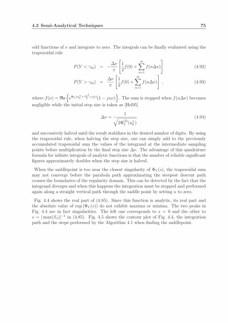
4.3 Semi-Analytical Techniques 75
odd functions of ν and integrate to zero. The integrals can be finally evaluated using thetrapezoidal rule
P (Y < γth) = −∆ν
π
[1
2f(0) +
∞∑
n=1
f(n∆ν)
](4.92)
P (Y > γth) =∆ν
π
[1
2f(0) +
∞∑
n=1
f(n∆ν)
], (4.93)
where f(ν) = Re
eΦY (u±
0 +κν2
2+jν)(1 − jκν)
. The sum is stopped when f(n∆ν) becomes
negligible while the initial step size is taken as [Hel95]
∆ν =1√
2Φ(2)Y (u±
0 )(4.94)
and successively halved until the result stabilizes in the desired number of digits. By usingthe trapezoidal rule, when halving the step size, one can simply add to the previouslyaccumulated trapezoidal sum the values of the integrand at the intermediate samplingpoints before multiplication by the final step size ∆ν. The advantage of this quadratureformula for infinite integrals of analytic functions is that the number of reliable significantfigures approximately doubles when the step size is halved.
When the saddlepoint is too near the closest singularity of ΦY (s), the trapezoidal summay not converge before the parabola path approximating the steepest descent pathcrosses the boundaries of the regularity domain. This can be detected by the fact that theintegrand diverges and when this happens the integration must be stopped and performedagain along a straight vertical path through the saddle point by setting κ to zero.
Fig. 4.4 shows the real part of (4.85). Since this function is analytic, its real part andthe absolute value of exp (ΦY (s)) do not exhibit maxima or minima. The two peaks inFig. 4.4 are in fact singularities. The left one corresponds to s = 0 and the other tos = |max(Sβ)|−1 in (4.85). Fig. 4.5 shows the contour plot of Fig. 4.4, the integrationpath and the steps performed by the Algorithm 4.1 when finding the saddlepoint.
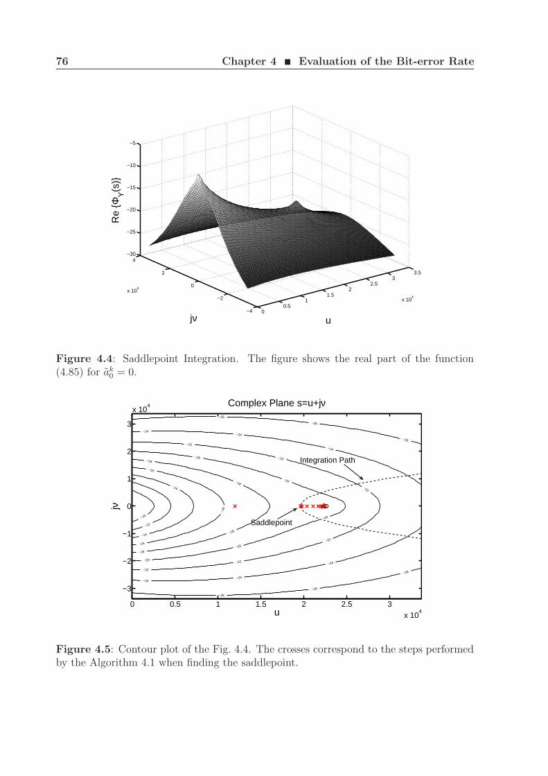
76 Chapter 4 ¥ Evaluation of the Bit-error Rate
00.5
11.5
22.5
33.5
x 104
−4
−2
0
2
4
x 104
−30
−25
−20
−15
−10
−5
ujν
Re
ΦY(s
)
Figure 4.4: Saddlepoint Integration. The figure shows the real part of the function(4.85) for ak
0 = 0.
−26
−26
−26
−26
−26
−26
−24−24
−24
−24−24
−24
−22
−22
−22
−22
−22
−22
−20
−20
−20
−20
−20
−18
−18
−18
−18
−18
−16
−16
−16
−14
−14
−12
−10
jν
Complex Plane s=u+jν
u0 0.5 1 1.5 2 2.5 3
x 104
−3
−2
−1
0
1
2
3
x 104
Saddlepoint
Integration Path
Figure 4.5: Contour plot of the Fig. 4.4. The crosses correspond to the steps performedby the Algorithm 4.1 when finding the saddlepoint.

4.3 Semi-Analytical Techniques 77
−3.5−3
−2.5−2
−1.5−1
−0.50
x 104
−4
−2
0
2
4
x 104
−30
−25
−20
−15
−10
−5
ujν
Re
ΦY(s
)
Figure 4.6: Saddlepoint Integration. The figure shows the real part of the function(4.85) for ak
0 = 1.
−26
−26
−26
−26
−26
−26
−24
−24
−24−24
−24
−24
−24−24
−22
−22
−22
−22
−22
−22
−20
−20
−20
−20
−20
−18
−18
−18
−16
−16
−16
−14
−14
−12
−10
u
jν
Complex Plane s=u+jν
−3 −2.5 −2 −1.5 −1 −0.5 0x 10
4
−3
−2
−1
0
1
2
3
x 104
Integration Path
Saddlepoint
Figure 4.7: Contour plot of the Fig. 4.4. The crosses correspond to the steps performedby the Algorithm 4.1 when finding the saddlepoint.
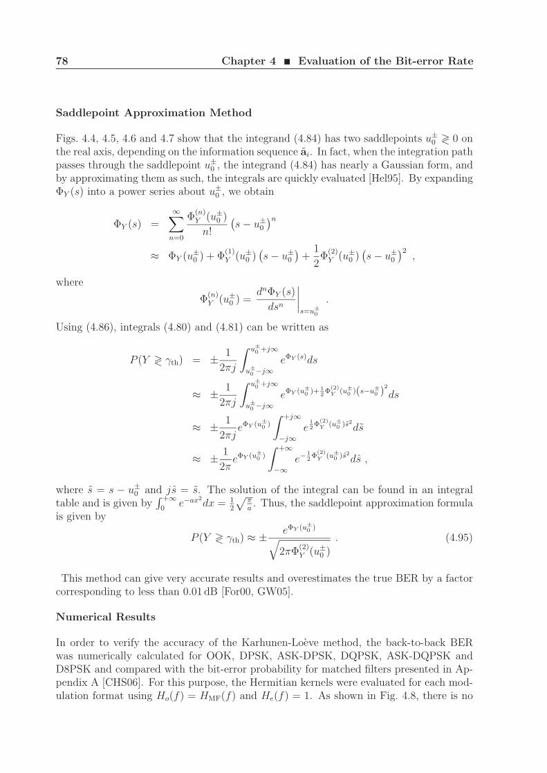
78 Chapter 4 ¥ Evaluation of the Bit-error Rate
Saddlepoint Approximation Method
Figs. 4.4, 4.5, 4.6 and 4.7 show that the integrand (4.84) has two saddlepoints u±0 ≷ 0 on
the real axis, depending on the information sequence ai. In fact, when the integration pathpasses through the saddlepoint u±
0 , the integrand (4.84) has nearly a Gaussian form, andby approximating them as such, the integrals are quickly evaluated [Hel95]. By expandingΦY (s) into a power series about u±
0 , we obtain
ΦY (s) =∞∑
n=0
Φ(n)Y (u±
0 )
n!
(s − u±
0
)n
≈ ΦY (u±0 ) + Φ
(1)Y (u±
0 )(s − u±
0
)+
1
2Φ
(2)Y (u±
0 )(s − u±
0
)2,
where
Φ(n)Y (u±
0 ) =dnΦY (s)
dsn
∣∣∣∣s=u±
0
.
Using (4.86), integrals (4.80) and (4.81) can be written as
P (Y ≷ γth) = ± 1
2πj
∫ u±
0 +j∞
u±
0 −j∞eΦY (s)ds
≈ ± 1
2πj
∫ u±
0 +j∞
u±
0 −j∞eΦY (u±
0 )+ 12Φ
(2)Y
(u±
0 )(s−u±
0 )2
ds
≈ ± 1
2πjeΦY (u±
0 )
∫ +j∞
−j∞e
12Φ
(2)Y
(u±
0 )s2
ds
≈ ± 1
2πeΦY (u±
0 )
∫ +∞
−∞e−
12Φ
(2)Y
(u±
0 )s2
ds ,
where s = s − u±0 and js = s. The solution of the integral can be found in an integral
table and is given by∫ +∞0
e−ax2dx = 1
2
√πa. Thus, the saddlepoint approximation formula
is given by
P (Y ≷ γth) ≈ ± eΦY (u±
0 )
√2πΦ
(2)Y (u±
0 ). (4.95)
This method can give very accurate results and overestimates the true BER by a factorcorresponding to less than 0.01 dB [For00, GW05].
Numerical Results
In order to verify the accuracy of the Karhunen-Loeve method, the back-to-back BERwas numerically calculated for OOK, DPSK, ASK-DPSK, DQPSK, ASK-DQPSK andD8PSK and compared with the bit-error probability for matched filters presented in Ap-pendix A [CHS06]. For this purpose, the Hermitian kernels were evaluated for each mod-ulation format using Ho(f) = HMF(f) and He(f) = 1. As shown in Fig. 4.8, there is no
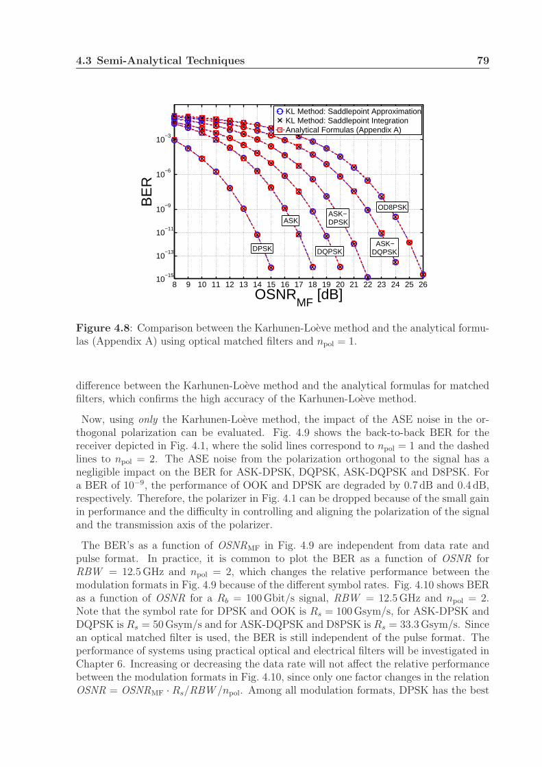
4.3 Semi-Analytical Techniques 79
8 9 10 11 12 13 14 15 16 17 18 19 20 21 22 23 24 25 2610
−15
10−13
10−11
10−9
10−6
10−3
OSNRMF
[dB]
BE
R
KL Method: Saddlepoint ApproximationKL Method: Saddlepoint IntegrationAnalytical Formulas (Appendix A)
ASK
DPSK
ASK−DPSK
ASK−DQPSKDQPSK
OD8PSK
Figure 4.8: Comparison between the Karhunen-Loeve method and the analytical formu-las (Appendix A) using optical matched filters and npol = 1.
difference between the Karhunen-Loeve method and the analytical formulas for matchedfilters, which confirms the high accuracy of the Karhunen-Loeve method.
Now, using only the Karhunen-Loeve method, the impact of the ASE noise in the or-thogonal polarization can be evaluated. Fig. 4.9 shows the back-to-back BER for thereceiver depicted in Fig. 4.1, where the solid lines correspond to npol = 1 and the dashedlines to npol = 2. The ASE noise from the polarization orthogonal to the signal has anegligible impact on the BER for ASK-DPSK, DQPSK, ASK-DQPSK and D8PSK. Fora BER of 10−9, the performance of OOK and DPSK are degraded by 0.7 dB and 0.4 dB,respectively. Therefore, the polarizer in Fig. 4.1 can be dropped because of the small gainin performance and the difficulty in controlling and aligning the polarization of the signaland the transmission axis of the polarizer.
The BER’s as a function of OSNRMF in Fig. 4.9 are independent from data rate andpulse format. In practice, it is common to plot the BER as a function of OSNR forRBW = 12.5 GHz and npol = 2, which changes the relative performance between themodulation formats in Fig. 4.9 because of the different symbol rates. Fig. 4.10 shows BERas a function of OSNR for a Rb = 100 Gbit/s signal, RBW = 12.5 GHz and npol = 2.Note that the symbol rate for DPSK and OOK is Rs = 100 Gsym/s, for ASK-DPSK andDQPSK is Rs = 50 Gsym/s and for ASK-DQPSK and D8PSK is Rs = 33.3 Gsym/s. Sincean optical matched filter is used, the BER is still independent of the pulse format. Theperformance of systems using practical optical and electrical filters will be investigated inChapter 6. Increasing or decreasing the data rate will not affect the relative performancebetween the modulation formats in Fig. 4.10, since only one factor changes in the relationOSNR = OSNRMF · Rs/RBW /npol. Among all modulation formats, DPSK has the best
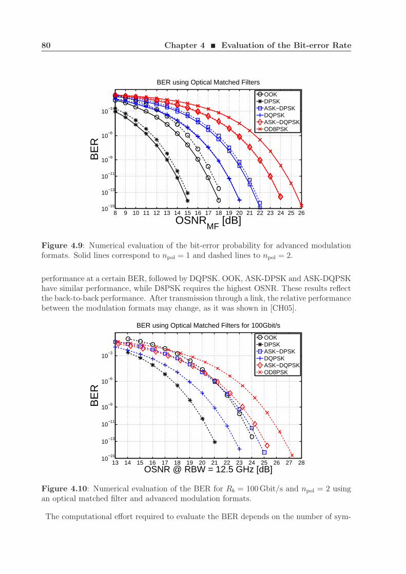
80 Chapter 4 ¥ Evaluation of the Bit-error Rate
8 9 10 11 12 13 14 15 16 17 18 19 20 21 22 23 24 25 2610
−15
10−13
10−11
10−9
10−6
10−3
OSNRMF
[dB]
BE
RBER using Optical Matched Filters
OOKDPSKASK−DPSKDQPSKASK−DQPSKOD8PSK
Figure 4.9: Numerical evaluation of the bit-error probability for advanced modulationformats. Solid lines correspond to npol = 1 and dashed lines to npol = 2.
performance at a certain BER, followed by DQPSK. OOK, ASK-DPSK and ASK-DQPSKhave similar performance, while D8PSK requires the highest OSNR. These results reflectthe back-to-back performance. After transmission through a link, the relative performancebetween the modulation formats may change, as it was shown in [CH05].
13 14 15 16 17 18 19 20 21 22 23 24 25 26 27 2810
−15
10−13
10−11
10−9
10−6
10−3
OSNR @ RBW = 12.5 GHz [dB]
BE
R
BER using Optical Matched Filters for 100Gbit/s
OOKDPSKASK−DPSKDQPSKASK−DQPSKOD8PSK
Figure 4.10: Numerical evaluation of the BER for Rb = 100 Gbit/s and npol = 2 usingan optical matched filter and advanced modulation formats.
The computational effort required to evaluate the BER depends on the number of sym-
4.3 Semi-Analytical Techniques 81
bols Nseq and samples per symbol. Considering a window of size Nw symbols, the bit-errorprobability can be calculated taking into account the interference of Nw − 1 neighboringsymbols. While the size of the window depends on the memory of the system, the numberof samples per symbol can be reduced in order to speed up the simulations. Fig.4.11 showsthe numerical evaluation of the BER for DPSK RZ-50% at Rb = 100 Gbit/s as a functionof the optical filter bandwidth Bo and the number of samples per symbol. Instead of anoptical matched filter a Gaussian optical filter of order no = 1 and a fifth-order Besselfilter of bandwidth Be = 75 GHz were used. The BER was evaluated for Nw = 3, npol = 1and OSNRMF = 13 dB. Increasing the window size does not significantly change the re-sults. Fig. 4.11 shows that five samples per symbol are enough to accurately evaluatethe BER, which corresponds to 15 eigenvalues [LS94, FS09]. The numerical evaluation ofthe signal propagation in the fiber, however, should use more than five samples per bitand a sequence large enough to take into account all nonlinear signal interactions. Atthe receiver, the signal can be down-sampled to five samples per bit and the BER can beevaluated in blocks of length Nw, for example.
4.3.2 Extended Karhunen-Loeve Expansion
The standard Karhunen-Loeve method assumes that the noise at the input of the balancedreceiver is white and Gaussian. Considering nonlinear phase noise the received noise isneither white nor Gaussian. However, if enough dispersion and filtering is present inthe system, the real and imaginary parts of the received noise can be approximated asGaussian, but not white. In fact, they are correlated and differently perturbed during thepropagation in the fiber. By separating in frequency domain the real and imaginary partsof the signal and noise, the impact of nonlinear phase noise on the BER can be evaluatedby combining the standard Karhunen-Loeve method with the system transmission matrixW(f). As shown in Fig. 4.3, the received signal is given by
A(f) = sout(f) + W(f)nN+1(f) (4.96)
and (4.71) and (4.72) can be rewritten as
I(tk) = eT
WKWeW , (4.97)
λi,W · qi,W = KW · qi,W , (4.98)
where eW and KW are a 4M × 1 column vector and a 4M × 4M matrix, respectively,given by
eW = W−1(f)
(ReesImes
)
︸ ︷︷ ︸eW,s
+
(ReenImen
)
︸ ︷︷ ︸eW,n
(4.99)
KW = WT(f)
(ReK −ImKImK ReK
)W(f) . (4.100)
The coefficients of the sum (4.65) are here given by si,W (tk) = qH
i,W · eW,s andni,W (tk) = qH
i,W · eW,n, where ni,W (tk), i = 1, 2, . . . , 4M , are zero-mean real Gaussian
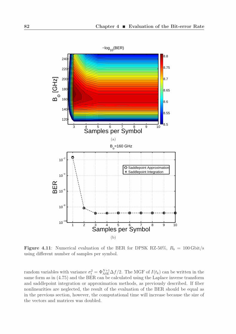
82 Chapter 4 ¥ Evaluation of the Bit-error Rate
Samples per Symbol
Bo [G
Hz]
−log10
(BER)
3 4 5 6 7 8 9 10
120
140
160
180
200
220
240
8.5
8.55
8.6
8.65
8.7
8.75
8.8
(a)
1 2 3 4 5 6 7 8 9 1010
−10
10−8
10−6
10−4
10−2
Samples per Symbol
BE
R
Bo=160 GHz
Saddlepoint ApproximationSaddlepoint Integration
(b)
Figure 4.11: Numerical evaluation of the BER for DPSK RZ-50%, Rb = 100 Gbit/susing different number of samples per symbol.
random variables with variance σ2t = ΦN+1
ASE ∆f/2. The MGF of I(tk) can be written in thesame form as in (4.75) and the BER can be calculated using the Laplace inverse transformand saddlepoint integration or approximation methods, as previously described. If fibernonlinearities are neglected, the result of the evaluation of the BER should be equal asin the previous section, however, the computational time will increase because the size ofthe vectors and matrices was doubled.
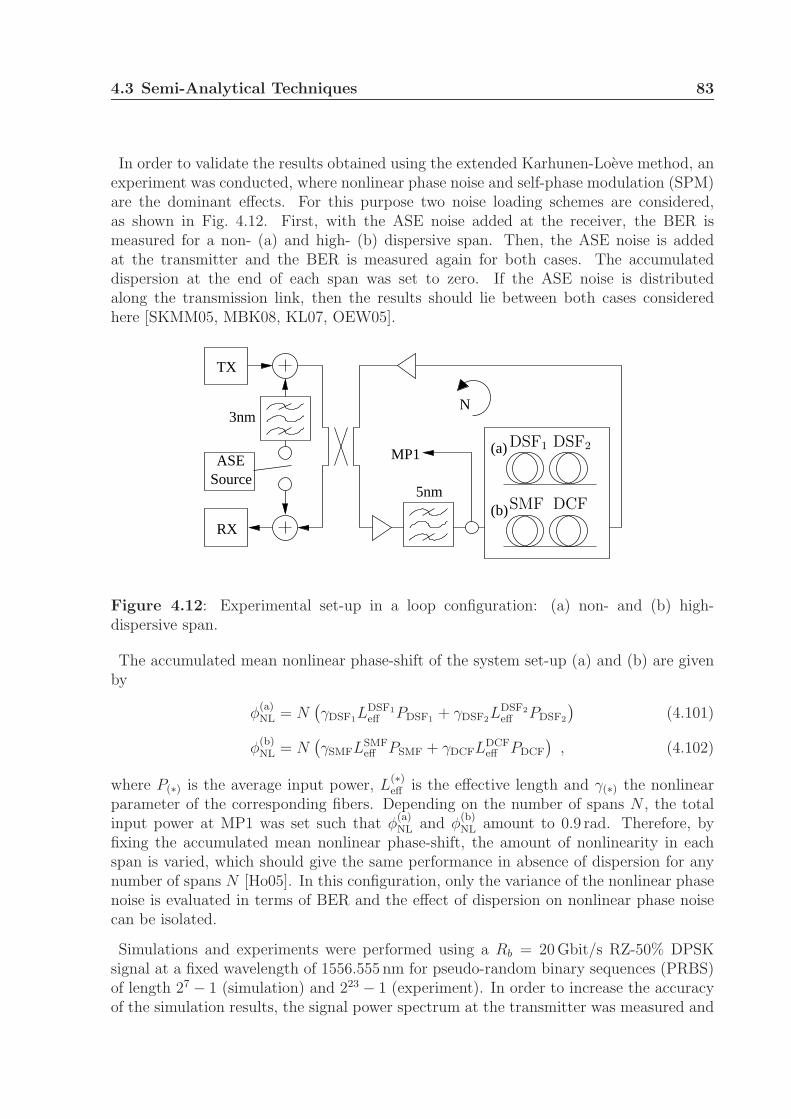
4.3 Semi-Analytical Techniques 83
In order to validate the results obtained using the extended Karhunen-Loeve method, anexperiment was conducted, where nonlinear phase noise and self-phase modulation (SPM)are the dominant effects. For this purpose two noise loading schemes are considered,as shown in Fig. 4.12. First, with the ASE noise added at the receiver, the BER ismeasured for a non- (a) and high- (b) dispersive span. Then, the ASE noise is addedat the transmitter and the BER is measured again for both cases. The accumulateddispersion at the end of each span was set to zero. If the ASE noise is distributedalong the transmission link, then the results should lie between both cases consideredhere [SKMM05, MBK08, KL07, OEW05].
N
ASE
TX
RX
3nm
5nm
MP1 (a)
(b)
Source
DSF2DSF1
DCFSMF
Figure 4.12: Experimental set-up in a loop configuration: (a) non- and (b) high-dispersive span.
The accumulated mean nonlinear phase-shift of the system set-up (a) and (b) are givenby
φ(a)NL = N
(γDSF1L
DSF1eff PDSF1 + γDSF2L
DSF2eff PDSF2
)(4.101)
φ(b)NL = N
(γSMFLSMF
eff PSMF + γDCFLDCFeff PDCF
), (4.102)
where P(∗) is the average input power, L(∗)eff is the effective length and γ(∗) the nonlinear
parameter of the corresponding fibers. Depending on the number of spans N , the totalinput power at MP1 was set such that φ
(a)NL and φ
(b)NL amount to 0.9 rad. Therefore, by
fixing the accumulated mean nonlinear phase-shift, the amount of nonlinearity in eachspan is varied, which should give the same performance in absence of dispersion for anynumber of spans N [Ho05]. In this configuration, only the variance of the nonlinear phasenoise is evaluated in terms of BER and the effect of dispersion on nonlinear phase noisecan be isolated.
Simulations and experiments were performed using a Rb = 20 Gbit/s RZ-50% DPSKsignal at a fixed wavelength of 1556.555 nm for pseudo-random binary sequences (PRBS)of length 27 − 1 (simulation) and 223 − 1 (experiment). In order to increase the accuracyof the simulation results, the signal power spectrum at the transmitter was measured and
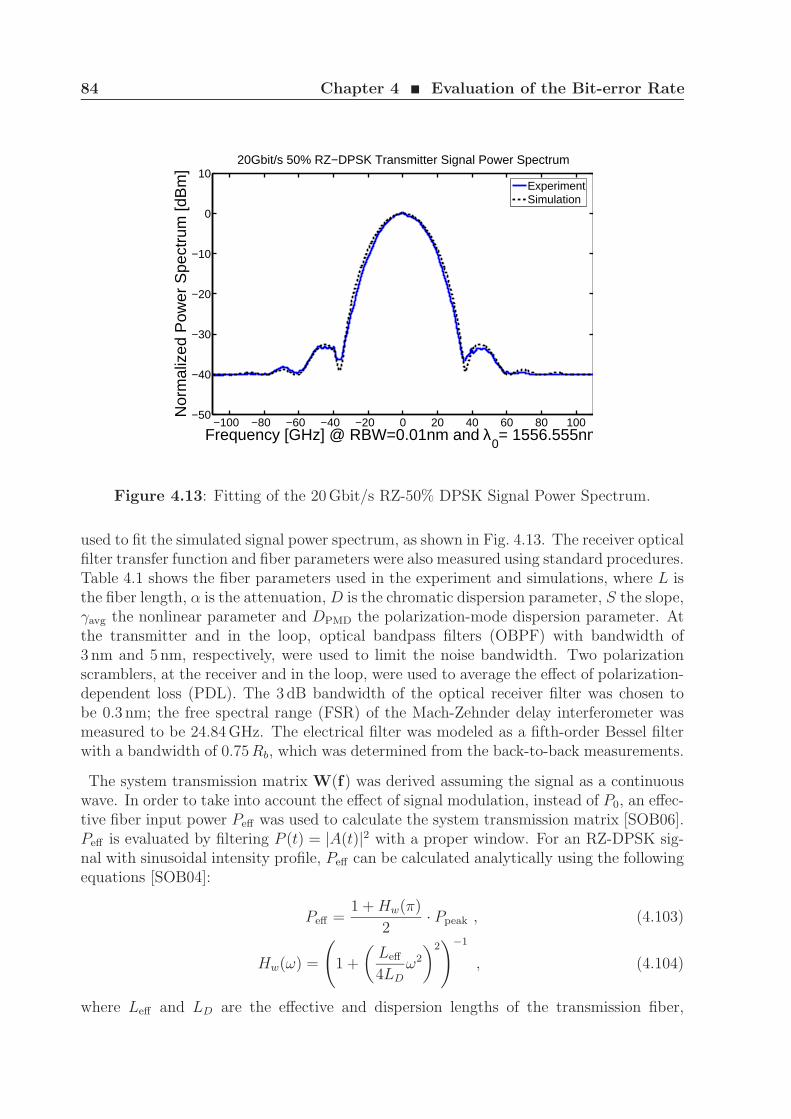
84 Chapter 4 ¥ Evaluation of the Bit-error Rate
−100 −80 −60 −40 −20 0 20 40 60 80 100−50
−40
−30
−20
−10
0
10
Frequency [GHz] @ RBW=0.01nm and λ0= 1556.555nm
Nor
mal
ized
Pow
er S
pect
rum
[dB
m]
20Gbit/s 50% RZ−DPSK Transmitter Signal Power Spectrum
ExperimentSimulation
Figure 4.13: Fitting of the 20 Gbit/s RZ-50% DPSK Signal Power Spectrum.
used to fit the simulated signal power spectrum, as shown in Fig. 4.13. The receiver opticalfilter transfer function and fiber parameters were also measured using standard procedures.Table 4.1 shows the fiber parameters used in the experiment and simulations, where L isthe fiber length, α is the attenuation, D is the chromatic dispersion parameter, S the slope,γavg the nonlinear parameter and DPMD the polarization-mode dispersion parameter. Atthe transmitter and in the loop, optical bandpass filters (OBPF) with bandwidth of3 nm and 5 nm, respectively, were used to limit the noise bandwidth. Two polarizationscramblers, at the receiver and in the loop, were used to average the effect of polarization-dependent loss (PDL). The 3 dB bandwidth of the optical receiver filter was chosen tobe 0.3 nm; the free spectral range (FSR) of the Mach-Zehnder delay interferometer wasmeasured to be 24.84 GHz. The electrical filter was modeled as a fifth-order Bessel filterwith a bandwidth of 0.75Rb, which was determined from the back-to-back measurements.
The system transmission matrix W(f) was derived assuming the signal as a continuouswave. In order to take into account the effect of signal modulation, instead of P0, an effec-tive fiber input power Peff was used to calculate the system transmission matrix [SOB06].Peff is evaluated by filtering P (t) = |A(t)|2 with a proper window. For an RZ-DPSK sig-nal with sinusoidal intensity profile, Peff can be calculated analytically using the followingequations [SOB04]:
Peff =1 + Hw(π)
2· Ppeak , (4.103)
Hw(ω) =
(1 +
(Leff
4LD
ω2
)2)−1
, (4.104)
where Leff and LD are the effective and dispersion lengths of the transmission fiber,
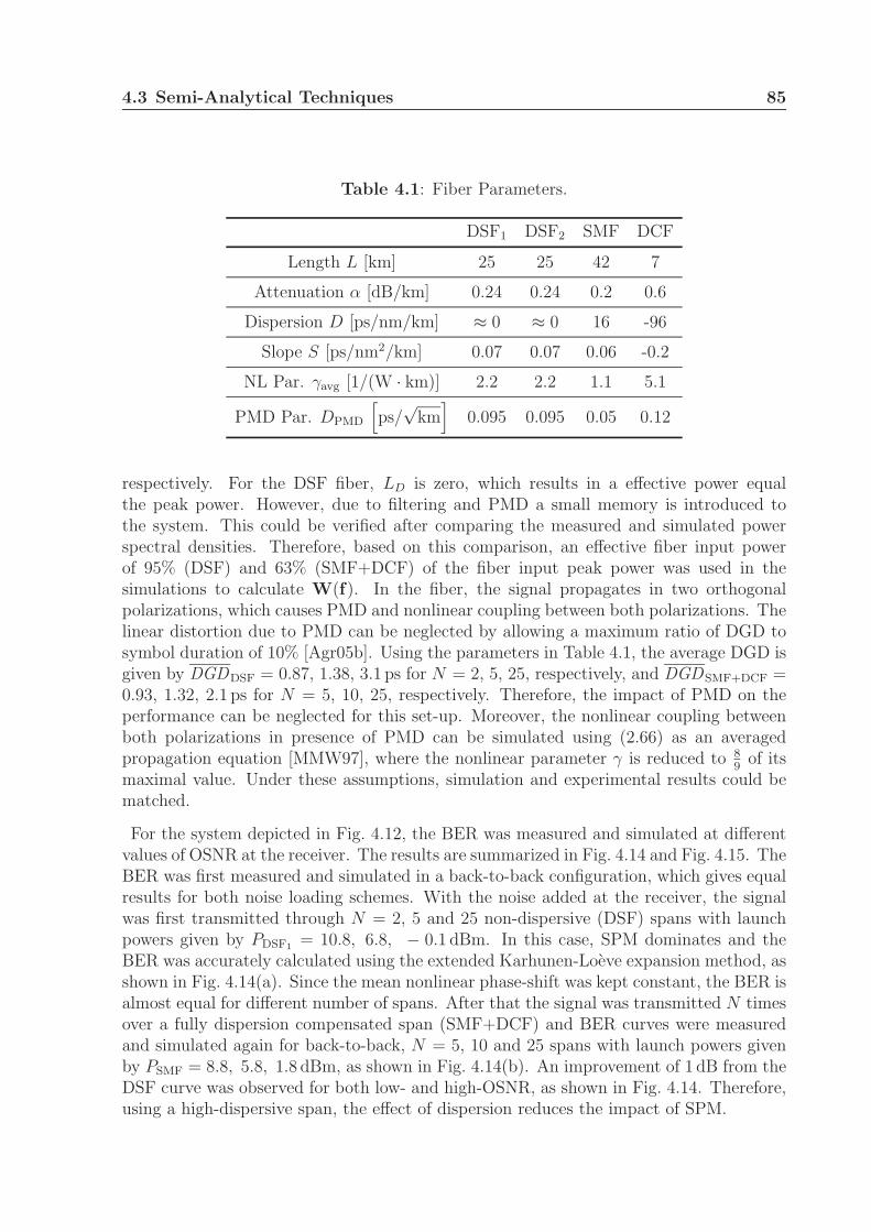
4.3 Semi-Analytical Techniques 85
Table 4.1: Fiber Parameters.
DSF1 DSF2 SMF DCF
Length L [km] 25 25 42 7
Attenuation α [dB/km] 0.24 0.24 0.2 0.6
Dispersion D [ps/nm/km] ≈ 0 ≈ 0 16 -96
Slope S [ps/nm2/km] 0.07 0.07 0.06 -0.2
NL Par. γavg [1/(W · km)] 2.2 2.2 1.1 5.1
PMD Par. DPMD
[ps/
√km
]0.095 0.095 0.05 0.12
respectively. For the DSF fiber, LD is zero, which results in a effective power equalthe peak power. However, due to filtering and PMD a small memory is introduced tothe system. This could be verified after comparing the measured and simulated powerspectral densities. Therefore, based on this comparison, an effective fiber input powerof 95% (DSF) and 63% (SMF+DCF) of the fiber input peak power was used in thesimulations to calculate W(f). In the fiber, the signal propagates in two orthogonalpolarizations, which causes PMD and nonlinear coupling between both polarizations. Thelinear distortion due to PMD can be neglected by allowing a maximum ratio of DGD tosymbol duration of 10% [Agr05b]. Using the parameters in Table 4.1, the average DGD isgiven by DGDDSF = 0.87, 1.38, 3.1 ps for N = 2, 5, 25, respectively, and DGDSMF+DCF =0.93, 1.32, 2.1 ps for N = 5, 10, 25, respectively. Therefore, the impact of PMD on theperformance can be neglected for this set-up. Moreover, the nonlinear coupling betweenboth polarizations in presence of PMD can be simulated using (2.66) as an averagedpropagation equation [MMW97], where the nonlinear parameter γ is reduced to 8
9of its
maximal value. Under these assumptions, simulation and experimental results could bematched.
For the system depicted in Fig. 4.12, the BER was measured and simulated at differentvalues of OSNR at the receiver. The results are summarized in Fig. 4.14 and Fig. 4.15. TheBER was first measured and simulated in a back-to-back configuration, which gives equalresults for both noise loading schemes. With the noise added at the receiver, the signalwas first transmitted through N = 2, 5 and 25 non-dispersive (DSF) spans with launchpowers given by PDSF1 = 10.8, 6.8, − 0.1 dBm. In this case, SPM dominates and theBER was accurately calculated using the extended Karhunen-Loeve expansion method, asshown in Fig. 4.14(a). Since the mean nonlinear phase-shift was kept constant, the BER isalmost equal for different number of spans. After that the signal was transmitted N timesover a fully dispersion compensated span (SMF+DCF) and BER curves were measuredand simulated again for back-to-back, N = 5, 10 and 25 spans with launch powers givenby PSMF = 8.8, 5.8, 1.8 dBm, as shown in Fig. 4.14(b). An improvement of 1 dB from theDSF curve was observed for both low- and high-OSNR, as shown in Fig. 4.14. Therefore,using a high-dispersive span, the effect of dispersion reduces the impact of SPM.
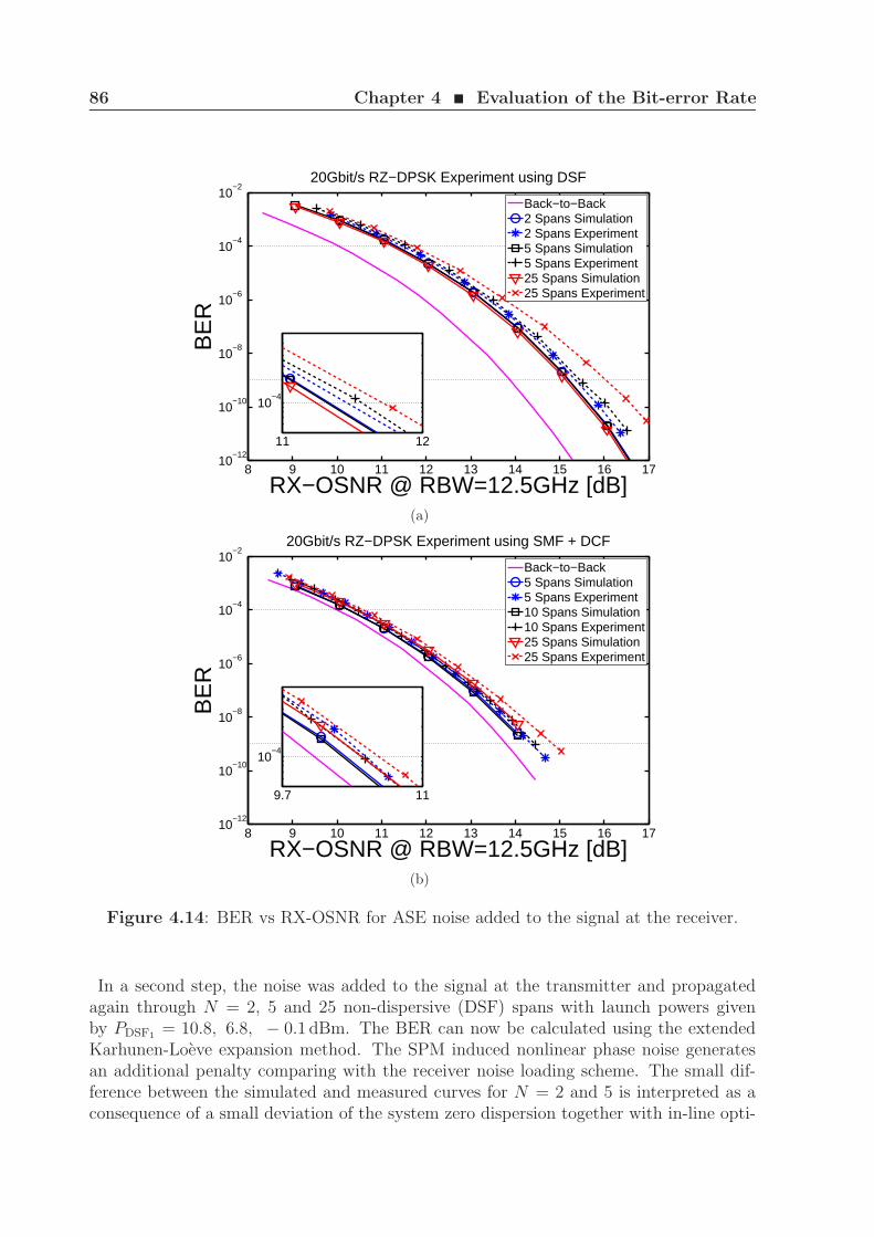
86 Chapter 4 ¥ Evaluation of the Bit-error Rate
8 9 10 11 12 13 14 15 16 1710
−12
10−10
10−8
10−6
10−4
10−2
RX−OSNR @ RBW=12.5GHz [dB]
BE
R20Gbit/s RZ−DPSK Experiment using DSF
Back−to−Back2 Spans Simulation2 Spans Experiment5 Spans Simulation5 Spans Experiment25 Spans Simulation25 Spans Experiment
11 12
10−4
(a)
8 9 10 11 12 13 14 15 16 1710
−12
10−10
10−8
10−6
10−4
10−2
RX−OSNR @ RBW=12.5GHz [dB]
BE
R
20Gbit/s RZ−DPSK Experiment using SMF + DCF
Back−to−Back5 Spans Simulation5 Spans Experiment10 Spans Simulation10 Spans Experiment25 Spans Simulation25 Spans Experiment
9.7 11
10−4
(b)
Figure 4.14: BER vs RX-OSNR for ASE noise added to the signal at the receiver.
In a second step, the noise was added to the signal at the transmitter and propagatedagain through N = 2, 5 and 25 non-dispersive (DSF) spans with launch powers givenby PDSF1 = 10.8, 6.8, − 0.1 dBm. The BER can now be calculated using the extendedKarhunen-Loeve expansion method. The SPM induced nonlinear phase noise generatesan additional penalty comparing with the receiver noise loading scheme. The small dif-ference between the simulated and measured curves for N = 2 and 5 is interpreted as aconsequence of a small deviation of the system zero dispersion together with in-line opti-
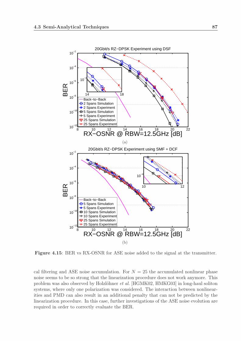
4.3 Semi-Analytical Techniques 87
8 10 12 14 16 18 20 2210
−12
10−10
10−8
10−6
10−4
10−2
RX−OSNR @ RBW=12.5GHz [dB]
BE
R
20Gbit/s RZ−DPSK Experiment using DSF
Back−to−Back2 Spans Simulation2 Spans Experiment5 Spans Simulation5 Spans Experiment25 Spans Simulation25 Spans Experiment
14 18
10−4
(a)
8 10 12 14 16 18 20 2210
−12
10−10
10−8
10−6
10−4
10−2
RX−OSNR @ RBW=12.5GHz [dB]
BE
R
20Gbit/s RZ−DPSK Experiment using SMF + DCF
Back−to−Back5 Spans Simulation5 Spans Experiment10 Spans Simulation10 Spans Experiment25 Spans Simulation25 Spans Experiment
10 12
10−4
(b)
Figure 4.15: BER vs RX-OSNR for ASE noise added to the signal at the transmitter.
cal filtering and ASE noise accumulation. For N = 25 the accumulated nonlinear phasenoise seems to be so strong that the linearization procedure does not work anymore. Thisproblem was also observed by Holzlohner et al. [HGMK02, HMKG03] in long-haul solitonsystems, where only one polarization was considered. The interaction between nonlinear-ities and PMD can also result in an additional penalty that can not be predicted by thelinearization procedure. In this case, further investigations of the ASE noise evolution arerequired in order to correctly evaluate the BER.
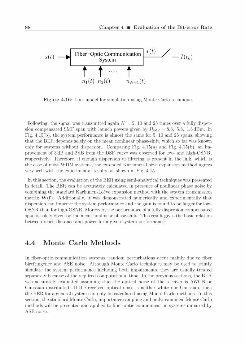
88 Chapter 4 ¥ Evaluation of the Bit-error Rate
Fiber−Optic CommunicationSystem I(tk)
n2(t)n1(t) nN+1(t)
s(t)I(t)
Figure 4.16: Link model for simulation using Monte Carlo techniques
Following, the signal was transmitted again N = 5, 10 and 25 times over a fully disper-sion compensated SMF span with launch powers given by PSMF = 8.8, 5.8, 1.8 dBm. InFig. 4.15(b), the system performance is almost the same for 5, 10 and 25 spans, showingthat the BER depends solely on the mean nonlinear phase-shift, which so far was knownonly for systems without dispersion. Comparing Fig. 4.15(a) and Fig. 4.15(b), an im-provement of 3 dB and 2 dB from the DSF curve was observed for low- and high-OSNR,respectively. Therefore, if enough dispersion or filtering is present in the link, which isthe case of most WDM systems, the extended Karhunen-Loeve expansion method agreesvery well with the experimental results, as shown in Fig. 4.15.
In this section, the evaluation of the BER using semi-analytical techniques was presentedin detail. The BER can be accurately calculated in presence of nonlinear phase noise bycombining the standard Karhunen-Loeve expansion method with the system transmissionmatrix W(f). Additionally, it was demonstrated numerically and experimentally thatdispersion can improve the system performance and the gain is found to be larger for low-OSNR than for high-OSNR. Moreover, the performance of a fully dispersion compensatedspan is solely given by the mean nonlinear phase-shift. This result gives the basic relationbetween reach-distance and power for a given system performance.
4.4 Monte Carlo Methods
In fiber-optic communication systems, random perturbations occur mainly due to fiberbirefringence and ASE noise. Although Monte Carlo techniques may be used to jointlysimulate the system performance including both impairments, they are usually treatedseparately because of the required computational time. In the previous sections, the BERwas accurately evaluated assuming that the optical noise at the receiver is AWGN orGaussian distributed. If the received optical noise is neither white nor Gaussian, thenthe BER for a general system can only be calculated using Monte Carlo methods. In thissection, the standard Monte Carlo, importance sampling and multi-canonical Monte Carlomethods will be presented and applied to fiber-optic communication systems impaired byASE noise.
4.4 Monte Carlo Methods 89
4.4.1 Standard Monte Carlo Simulation
Besides all linear and nonlinear effects, the propagation of an optical signal through a linkis also impaired by several noise sources, which limits the maximum amount of informationthat can be transmitted. Numerical simulation of these systems requires the generationof a significant number of noisy waveforms, in order to accurately estimate the systemperformance. Fig. 4.16 shows a fiber-optic communication system, where s(t) is an opticalsignal and n1(t), n2(t), . . . , nN+1(t) are ASE noise sources. The demodulated signalI(t) is a nonlinear function of the signal and ASE noise sources. The statistical propertiesof I(t) can be estimated by emulating the system including the time evolution of allthe waveforms in the system. This implies generating sampled values of all the inputprocesses, propagating the signal and noise through the link, and observing the outputwaveforms. This technique and its variants are known as Monte Carlo methods. Ideally,the Monte Carlo simulation corresponds to the real system within the limits of modelingassumptions and approximations [JBS00].
Consider the decision random variable Y = I(tk) = g(X), where g : Γ → R is a realscalar nonlinear function of a random vector X, which assumes values in the samplespace Γ [BRG+09]. The PDF of Y , pY (y), can be estimated by drawing samples fromthe joint PDF pX(x) and evaluating y = g(x). A given interval B = [ymin, ymax] ⊂ Ris divided into Nb bins Bi =
[yi − ∆y
2, yi + ∆y
2
]of width ∆y = ymax−ymin
Nb, where yi =
ymin +(i − 1
2
)· ∆y. This partition also divides the sample space Γ into Nb subspaces,
whereΓi = x ∈ Γ | g(x) ∈ Bi (4.105)
is the domain in Γ that maps into the i-th bin. Note that Γi are multi-dimensional regions,while Bi are simple intervals. The probability that a sample falls in the i-th bin is givenby
PrY ∈ Bi = PY (Bi) =
∫ yi+∆y
2
yi−∆y
2
pY (y)dy =
∫ ∞
−∞χi(Y ) pY (y)dy = EpY
χi(Y ) , (4.106)
where
χi(Y ) =
1 if Y ∈ Bi
0 otherwise. (4.107)
The probability PY (Bi) can also be written in terms of X as
PY (Bi) =
∫
Γi
pX(x)dx =
∫
Γ
χi(X)pX(x)dx = EpXχi(X) , (4.108)
where
χi(X) =
1 if X ∈ Γi
0 otherwise. (4.109)
Each probability PY (Bi) can be estimated using the sample mean as
PY (Bi) ≈1
Ns
Ns∑
l=1
χi(g(xl)) =Ni
Ns
, (4.110)
90 Chapter 4 ¥ Evaluation of the Bit-error Rate
where Ns are samples from the distribution pX(x) and Ni is the number of samples thatfall in Bi. The probability mass function (PMF) of the discretized Y is given by theset PY (B1), PY (B2), . . . , PY (BNb
)) and can be written as a function of the continuousvariable y as
PrY = y , PPMFY (y) =
Nb∑
i=1
rect
(y − yi
∆y
)· PY (Bi) , (4.111)
where rect(
y
a
)= u
(y + a
2
)− u
(y − a
2
)is the rectangular function and u(y) is the unit
step function. Using the approximation PY (Bi) ≈ pY (yi) · ∆y, the PDF of Y can beestimated as
pY (y) =PPMF
Y (y)
∆y=
1
∆y
Nb∑
i=1
rect
(y − yi
∆y
)· PY (Bi) . (4.112)
The accuracy of the PDF estimation is usually given by the relative error [SB80, Jer84]
εi =
√VarPY (Bi)E2PY (Bi)
=
√PY (Bi)(1 − PY (Bi))
(PY (Bi))2Ns
≈ 1√PY (Bi)Ns
, (4.113)
where the expected value and variance of the estimator PY (Bi) are given by EPY (Bi) =PY (Bi) and
VarPY (Bi) = E(PY (Bi))2 − E2PY (Bi)
= E
(1
Ns
Ns∑
l=1
χi(g(xl))
)2 − (PY (Bi))
2
=1
N2s
E
Ns∑
l=1
Ns∑
m=1
χi(g(xl)) χi(g(xm))
− (PY (Bi))
2
=1
N2s
Ns PY (Bi) +2
N2s
Ns−1∑
l=1
Ns∑
m=l+1
E χi(g(xl))E χi(g(xm)) − (PY (Bi))2
=PY (Bi)
Ns
+2
N2s
· (PY (Bi))2 · N2
s − Ns
2− (PY (Bi))
2
=PY (Bi)(1 − PY (Bi))
Ns
, (4.114)
respectively. In a standard Monte Carlo simulation, most of the samples fall in bins closeto the expected value, while less samples will fall on the regions of interest, the tails ofthe PDF. For a given maximum relative error in each bin εi, the number of requiredsamples Ns increases inversely proportional to PY (Bi), and, thus, to the BER. This isthe reason why standard Monte Carlo is so time-consuming. Therefore, for low BER,importance sampling and multi-canonical techniques are more efficient than standardMonte Carlo simulation.
4.4 Monte Carlo Methods 91
4.4.2 Importance Sampling
The idea of importance sampling (IS) is to modify the generation of samples in such away that the number of samples falling in the tails of the PDF pY (y) increases. An ISestimator can be calculated by rewriting (4.108) as
PY (Bi) =
∫
Γ
χi(X)pX(x)
p∗X(x)p∗X(x)dx =
∫
Γ
χi(X) w(x) p∗X(x)dx (4.115)
= Ep∗Xχi(X) w(x) , (4.116)
where w(x) is the IS weight. The new PDF p∗Y (y) is created by drawing samples accordingto the biasing PDF p∗X(x) instead of pX(x). Each probability PY (Bi) can be estimatedby calculating
PY (Bi) ≈ 1
Ns
Ns∑
l=1
χi(g(xl))pX(xl)
p∗X(xl)=
1
Ns
Ns∑
l=1
χi(g(xl)) w(xl) (4.117)
=N∗
i
Ns
· 1
N∗i
N∗i∑
l=1
w(xl)
︸ ︷︷ ︸wi
, (4.118)
where N∗i is the number of samples generated from p∗X(x) that fall in Bi. The main disad-
vantage of the importance sampling technique is that the choice of a biasing distributionrequires some knowledge of which noise samples most likely fall on the PDF tails. Thisproblem can be avoided by using the multi-canonical Monte Carlo technique describednext.
4.4.3 Multi-Canonical Monte Carlo Simulation
The accuracy of the estimation using the standard Monte Carlo method depends on thenumber of samples Ns, the higher, the better is the estimation. Another way to improvethe BER estimation is the biased generation of noisy waveforms, which aims to producea sufficient number of events in the tails of the PDF, as previously discussed. However,finding the optimal biasing requires a previous knowledge of the system, which is notalways feasible. By adaptively forming the biasing distribution, the output distributionof a system pY (y) and, therefore, the BER can be estimated in a feasible computationaltime without knowing details about the system configuration. This method is known asmulti-canonical Monte Carlo (MMC) and it is widely used for calculating the probabilityof rare events.
In (4.117), the optimal biasing distribution for the i-th bin is given by
p∗X,opt(x) =χi(g(xl))
PY (Bi)pX(x) . (4.119)
Since PY (Bi) is the quantity to be estimated, the optimal distribution is initially un-known. In importance sampling, the biasing distribution is chosen such that p∗X(x) is
92 Chapter 4 ¥ Evaluation of the Bit-error Rate
close to p∗X,opt(x), while the MMC method determines p∗X,opt(x) iteratively. The biasingdistribution at iteration n can be written as
p∗,nX (x) =1
cn−1 P n−1Y (Bi)
pX(x) , (4.120)
where cn−1 is an unknown constant, which guarantees that∫
Γp∗,nX (x)dx = 1. By substi-
tuting (4.120) in (4.117), the probability of each bin at the iteration n is given by
P nY (Bi) =
1
Ns
Ns∑
l=1
χi(g(xl))pX(xl)
p∗,nX (xl)
= cn−1P n−1Y (Bi) ·
1
Ns
Ns∑
l=1
χi(g(xl))
= cn−1P n−1Y (Bi) ·
N∗,ni
Ns
, (4.121)
where wni = cn−1P n−1
Y (Bi). Using∑Nb
i=1 P n−1Y (Bi) = 1, the constant cn−1 can be calculated
as
cn−1 =
(Nb∑
i=1
P n−1Y (Bi) ·
N∗,ni
Ns
)−1
. (4.122)
To avoid division by zero in (4.120), N∗,ni can be substituted by N∗,n
i + 1 in (4.121) andthe estimated probability of each bin can be written as
P nY (Bi) = cn−1P n−1
Y (Bi) ·N∗,n
i + 1
Ns
, (4.123)
where the constant cn−1 is calculated in the same manner as cn−1, but using N∗,ni + 1
instead of N∗,ni . At the first iteration n = 1, the initial values are set to c0 = Nb and
P 0Y (Bi) = 1
Nb, which corresponds to a standard Monte Carlo simulation. After a certain
number of iterations, the expected number of samples in each bin converges to Ns/Nb
and is independent of i [HM03]. Substituting this value in (4.117) results in cn → Nb andP n
Y (Bi) → PY (Bi).
The estimation of the PDF using the MMC method can be further improved by using asmoothing technique introduced by Berg [BN91, BN92, Ber98, Ber99]. In this case, theprobability P n
Y (Bi+1) is given by
P nY (Bi+1) =
P nY (Bi) P n−1
Y (Bi+1)
P n−1Y (Bi)
(N∗,n
i+1
N∗,ni
)gni
, (4.124)
where
gni =
gni∑n
l=1 gli
, gli =
N∗,li N∗,l
i+1
N∗,li + N∗,l
i+1
(4.125)
4.4 Monte Carlo Methods 93
and P nY (B1) = P n−1
Y (B1). After calculating the probability for all bins, a normalization
should be performed on all P nY (Bi) such that
∑Nb
i=1 P nY (Bi) = 1. Moreover, using Berg’s
update, the division by zero in (4.120) is avoided by setting initially P 0Y (Bi) = 1
Nb. For
the case where N∗,ni , N∗,n
i+1 or both equal zero, P nY (Bi+1) is defined as
P nY (Bi+1) =
P nY (Bi) P n−1
Y (Bi+1)
P n−1Y (Bi)
, (4.126)
which causes a propagation of the values of bin i − 1 to bin i.
The Metropolis Algorithm
It is common to find software routines for generation of random samples with an uni-form or Gaussian distribution. However, an important part of the MMC method is thegeneration of samples from an arbitrary probability distribution p∗,nX (x). The Metropolisalgorithm [MU49, MRR+53] is a Markov-Chain Monte Carlo (MCMC) method, which iswidely used to obtain random samples from a general distribution. The algorithm gen-erates a random walk of correlated samples x1, x2, . . . ,xl, . . ., whose distribution atequilibrium equals the desired PDF p∗,nX (x).
At run l of the iteration n, the next sample is proposed as
xprop = xcurr + hn · ∆x (4.127)
where xcurr = xl is the current sample, ∆x is a symmetric uniformly distributed randomvector over the interval [−0.5, 0.5] and hn controls the variance of ∆x, which is a keyparameter in the MMC method. In order to determine the bin corresponding to the pro-posed sample Bi=p, p ∈ 1, 2, . . . , Nb, the algorithm evaluates yprop = g(xprop). Note thatin the previous run l−1, the algorithm evaluated ycurr = g(xcurr) and also determined thebin corresponding to the sample xcurr, Bi=c, c ∈ 1, 2, . . . , Nb. Therefore, the proposedsample is accepted with a probability [HM03]
Pprop = min
(p∗,nX (xprop)
p∗,nX (xcurr), 1
)= min
( 1
cn−1 P n−1Y
(Bi=p)pX(xprop)
1
cn−1 P n−1Y
(Bi=c)pX(xcurr)
, 1
)
= min
(pX(xprop)
pX(xcurr)
P n−1Y (Bi=c)
P n−1Y (Bi=p)
, 1
), (4.128)
The distribution pX(x) is known and so are pX(xprop) and pX(xl). If the proposedsample is accepted, then xl+1 = xprop and N∗,n
i=p = N∗,ni=p + 1. Otherwise, if the proposed
sample is rejected, then xl+1 = xcurr and N∗,ni=c = N∗,n
i=c + 1. Note that in this method theconstant cn and the region Γi do not need to be calculated, which drastically reduces thecomputational effort. In this way, samples are generated from the PDF p∗,nX (x) and thePDF of Y, pY (y), can be estimated and also the BER. The Algorithm 4.2 summarizes theMMC method, where Nit is the number of iterations.
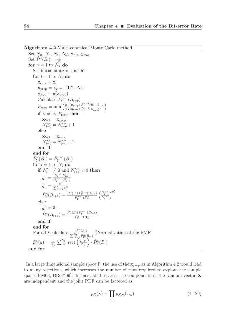
94 Chapter 4 ¥ Evaluation of the Bit-error Rate
Algorithm 4.2 Multi-canonical Monte Carlo methodSet Nit, Ns, Nb, ∆y, ymin, ymax
Set P 0Y (Bi) = 1
Nb
for n = 1 to Nit doSet initial state x1 and hn
for l = 1 to Ns doxcurr = xl
xprop = xcurr + hn · ∆xyprop = g(xprop)
Calculate P n−1Y (Bi=p)
Pprop = min(
pX(xprop)
pX(xcurr)
P n−1Y
(Bi=c)
P n−1Y
(Bi=p), 1
)
if rand < Pprop thenxl+1 = xprop
N∗,ni=p = N∗,n
i=p + 1else
xl+1 = xcurr
N∗,ni=c = N∗,n
i=c + 1end if
end forP n
Y (B1) = P n−1Y (B1)
for i = 1 to Nb doif N∗,n
i 6= 0 and N∗,ni+1 6= 0 then
gni =
N∗,ni N
∗,ni+1
N∗,ni +N
∗,ni+1
gni =
gni∑n
m=1 gmi
P nY (Bi+1) =
P nY
(Bi) P n−1Y
(Bi+1)
P n−1Y
(Bi)
(N
∗,ni+1
N∗,ni
)gni
elsegn
i = 0
P nY (Bi+1) =
P nY
(Bi) P n−1Y
(Bi+1)
P n−1Y
(Bi)
end ifend forFor all i calculate
P nY
(Bi)∑Nbm=1 P n
Y(Bm)
Normalization of the PMF
pnY (y) = 1
∆y
∑Nb
i=1 rect(
y−yi
∆y
)· P n
Y (Bi)
end for
In a large dimensional sample space Γ, the use of the xprop as in Algorithm 4.2 would leadto many rejections, which increases the number of runs required to explore the samplespace [HM03, BRG+09]. In most of the cases, the components of the random vector Xare independent and the joint PDF can be factored as
pX(x) =∏
m
pX,m(xm) (4.129)
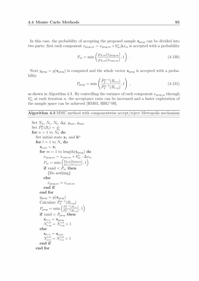
4.4 Monte Carlo Methods 95
In this case, the probability of accepting the proposed sample xprop can be divided intotwo parts: first each component xprop,m = xprop,m +hn
m∆xm is accepted with a probability
Pm = min
(pX,m(xprop,m)
pX,m(xcurr,m), 1
). (4.130)
Next yprop = g(xprop) is computed and the whole vector xprop is accepted with a proba-bility
Pprop = min
(P n−1
Y (Bi=c)
P n−1Y (Bi=p)
, 1
), (4.131)
as shown in Algorithm 4.3. By controlling the variance of each component xprop,m throughhn
m at each iteration n, the acceptance ratio can be increased and a faster exploration ofthe sample space can be achieved [HM03, BRG+09].
Algorithm 4.3 MMC method with componentwise accept/reject Metropolis mechanism
Set Nit, Ns, Nb, ∆y, ymin, ymax
Set P 0Y (Bi) = 1
Nb
for n = 1 to Nit doSet initial state x1 and hn
for l = 1 to Ns doxcurr = xl
for m = 1 to length(xprop) doxprop,m = xcurr,m + hn
m · ∆xm
Pm = min(
pX,m(xprop,m)
pX,m(xcurr,m), 1
)
if rand < Pm thenDo nothing
elsexprop,m = xcurr,m
end ifend foryprop = g(xprop)
Calculate P n−1Y (Bi=p)
Pprop = min(
P n−1Y
(Bi=c)
P n−1Y
(Bi=p), 1
)
if rand < Pprop thenxl+1 = xprop
N∗,ni=p = N∗,n
i=p + 1else
xl+1 = xcurr
N∗,ni=c = N∗,n
i=c + 1end if
end for
96 Chapter 4 ¥ Evaluation of the Bit-error Rate
P nY (B1) = P n−1
Y (B1)for i = 1 to Nb do
if N∗,ni 6= 0 and N∗,n
i+1 6= 0 then
gni =
N∗,ni N
∗,ni+1
N∗,ni +N
∗,ni+1
gni =
gni∑n
m=1 gmi
P nY (Bi+1) =
P nY
(Bi) P n−1Y
(Bi+1)
P n−1Y
(Bi)
(N
∗,ni+1
N∗,ni
)gni
elsegn
i = 0
P nY (Bi+1) =
P nY
(Bi) P n−1Y
(Bi+1)
P n−1Y
(Bi)
end ifend for
For all i calculateP n
Y(Bi)∑Nb
m=1 P nY
(Bm)Normalization of the PMF
pnY (y) = 1
∆y
∑Nb
i=1 rect(
y−yi
∆y
)· P n
Y (Bi)
end for
4.4.4 Noise realization in the frequency domain
The simulation time of both standard and multi-canonical Monte Carlo methods canbe significantly reduced by generating the ASE noise samples in the frequency domain.In fiber-optic communication systems, each ASE noise source is usually expressed as acontinuous AWGN process in time domain. By sampling this process M times, the noisevector is given by
n = [n0, n1, . . . , nM−1]T = [nre
0 , nre1 , . . . , nre
M−1]T + j[nim
0 , nim1 , . . . , nim
M−1]T , (4.132)
where each component nm is a zero-mean complex Gaussian random variable with inde-pendent real and imaginary components of variance σ2
t = ΦASE∆f/2. The samples areequally spaced by ∆t and ∆f in time and frequency domain, respectively, and coincidewith the discrete frequency vector of the DFT. ΦASE is the power spectral density of theASE noise in one polarization. The vector n can be expressed in frequency domain usingthe DFT as
n = WDFT · n =
w0·0M w0·1
M · · · w0·(M−1)M
w1·0M w1·1
M · · · w1·(M−1)M
......
. . ....
w(M−1)·0M w
(M−1)·1M · · · w
(M−1)·(M−1)M
·
n0
n1...
nM−1
, (4.133)
where WDFT is the DFT matrix and wM = exp (−2πj/M). Since the DFT matrix is alinear transformation, the noise n is also a zero-mean complex Gaussian random variablewith independent real and imaginary components of variance σ2
f . The covariance matrix
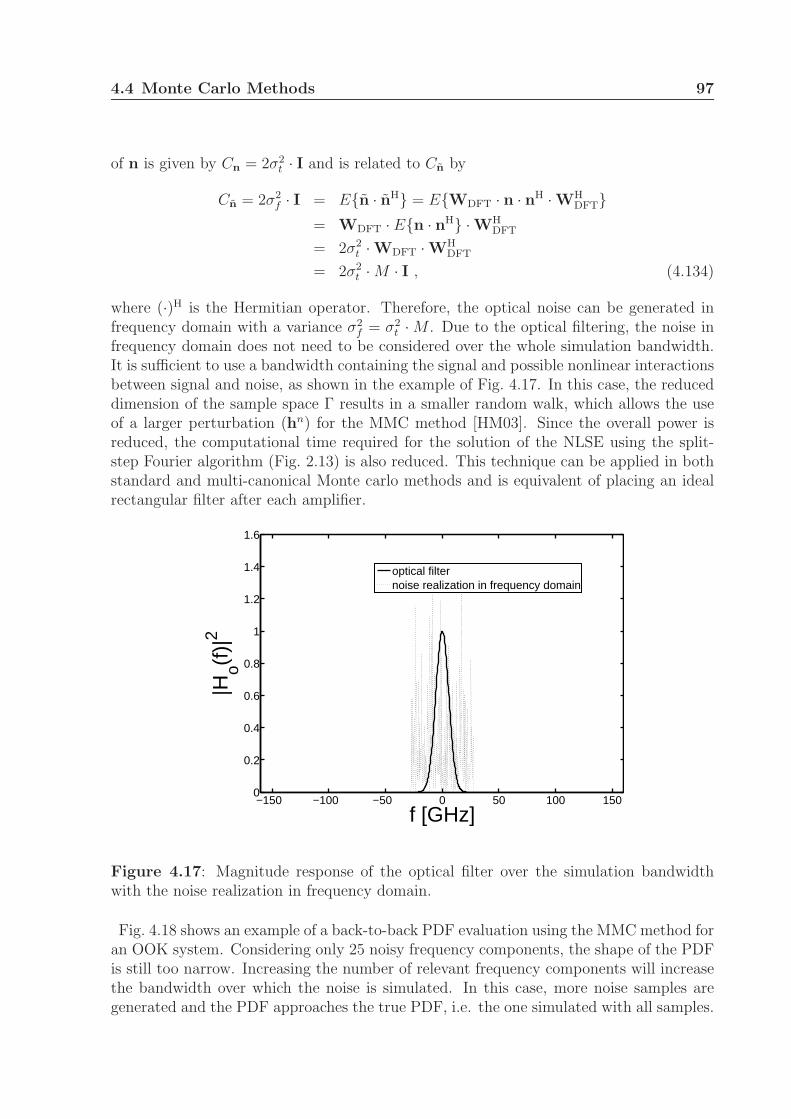
4.4 Monte Carlo Methods 97
of n is given by Cn = 2σ2t · I and is related to Cn by
Cn = 2σ2f · I = En · nH = EWDFT · n · nH · WH
DFT= WDFT · En · nH · WH
DFT
= 2σ2t · WDFT · WH
DFT
= 2σ2t · M · I , (4.134)
where (·)H is the Hermitian operator. Therefore, the optical noise can be generated infrequency domain with a variance σ2
f = σ2t · M . Due to the optical filtering, the noise in
frequency domain does not need to be considered over the whole simulation bandwidth.It is sufficient to use a bandwidth containing the signal and possible nonlinear interactionsbetween signal and noise, as shown in the example of Fig. 4.17. In this case, the reduceddimension of the sample space Γ results in a smaller random walk, which allows the useof a larger perturbation (hn) for the MMC method [HM03]. Since the overall power isreduced, the computational time required for the solution of the NLSE using the split-step Fourier algorithm (Fig. 2.13) is also reduced. This technique can be applied in bothstandard and multi-canonical Monte carlo methods and is equivalent of placing an idealrectangular filter after each amplifier.
−150 −100 −50 0 50 100 1500
0.2
0.4
0.6
0.8
1
1.2
1.4
1.6
f [GHz]
|Ho(f
)|2
optical filternoise realization in frequency domain
Figure 4.17: Magnitude response of the optical filter over the simulation bandwidthwith the noise realization in frequency domain.
Fig. 4.18 shows an example of a back-to-back PDF evaluation using the MMC method foran OOK system. Considering only 25 noisy frequency components, the shape of the PDFis still too narrow. Increasing the number of relevant frequency components will increasethe bandwidth over which the noise is simulated. In this case, more noise samples aregenerated and the PDF approaches the true PDF, i.e. the one simulated with all samples.
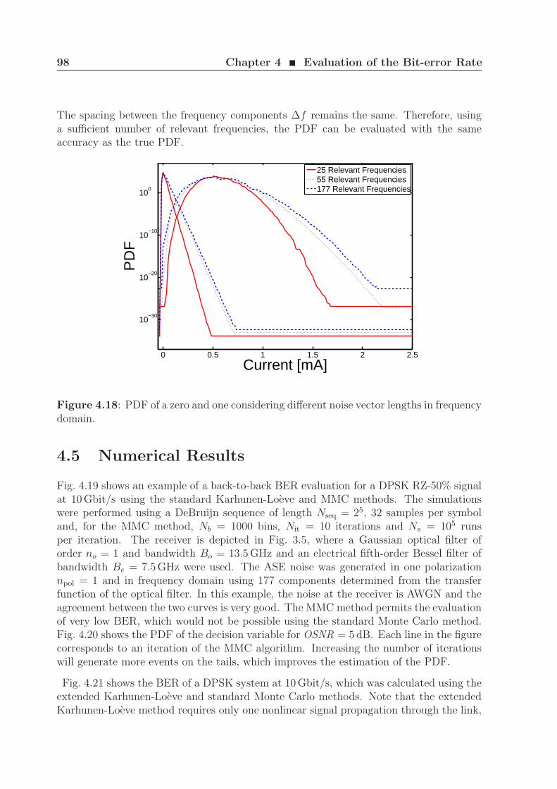
98 Chapter 4 ¥ Evaluation of the Bit-error Rate
The spacing between the frequency components ∆f remains the same. Therefore, usinga sufficient number of relevant frequencies, the PDF can be evaluated with the sameaccuracy as the true PDF.
0 0.5 1 1.5 2 2.5
10−30
10−20
10−10
100
Current [mA]
PD
F
25 Relevant Frequencies55 Relevant Frequencies177 Relevant Frequencies
Figure 4.18: PDF of a zero and one considering different noise vector lengths in frequencydomain.
4.5 Numerical Results
Fig. 4.19 shows an example of a back-to-back BER evaluation for a DPSK RZ-50% signalat 10 Gbit/s using the standard Karhunen-Loeve and MMC methods. The simulationswere performed using a DeBruijn sequence of length Nseq = 25, 32 samples per symboland, for the MMC method, Nb = 1000 bins, Nit = 10 iterations and Ns = 105 runsper iteration. The receiver is depicted in Fig. 3.5, where a Gaussian optical filter oforder no = 1 and bandwidth Bo = 13.5 GHz and an electrical fifth-order Bessel filter ofbandwidth Be = 7.5 GHz were used. The ASE noise was generated in one polarizationnpol = 1 and in frequency domain using 177 components determined from the transferfunction of the optical filter. In this example, the noise at the receiver is AWGN and theagreement between the two curves is very good. The MMC method permits the evaluationof very low BER, which would not be possible using the standard Monte Carlo method.Fig. 4.20 shows the PDF of the decision variable for OSNR = 5 dB. Each line in the figurecorresponds to an iteration of the MMC algorithm. Increasing the number of iterationswill generate more events on the tails, which improves the estimation of the PDF.
Fig. 4.21 shows the BER of a DPSK system at 10 Gbit/s, which was calculated using theextended Karhunen-Loeve and standard Monte Carlo methods. Note that the extendedKarhunen-Loeve method requires only one nonlinear signal propagation through the link,
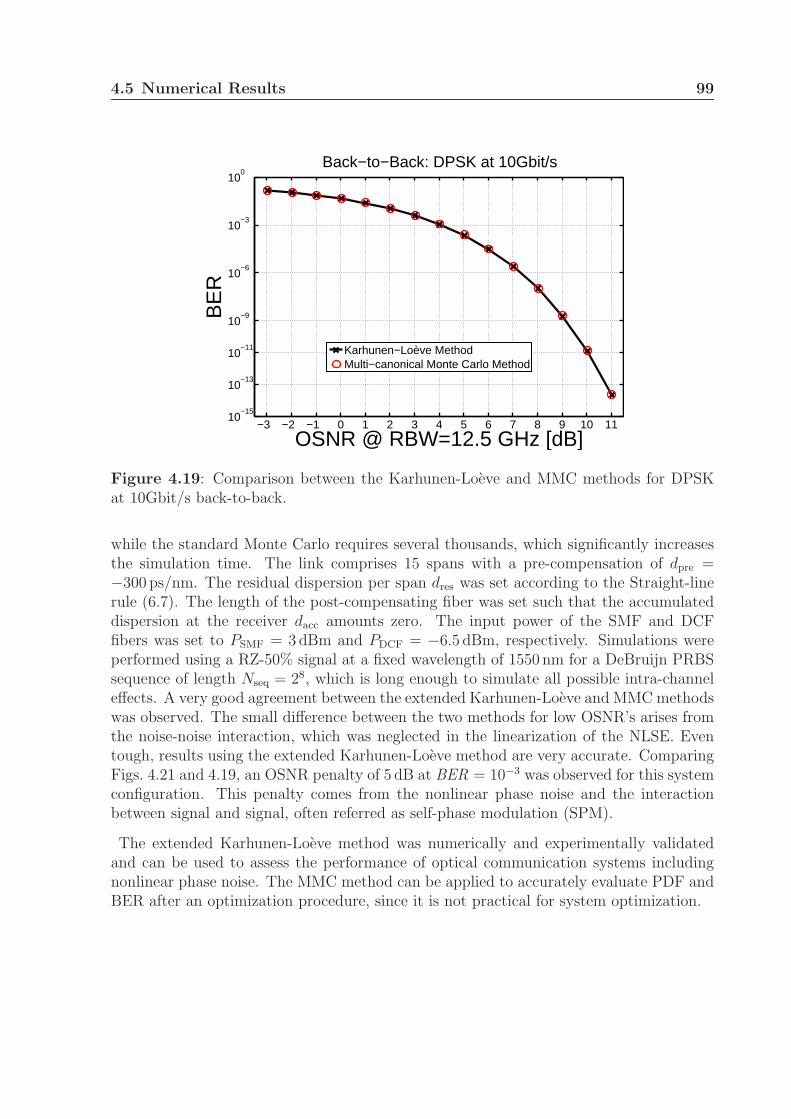
4.5 Numerical Results 99
−3 −2 −1 0 1 2 3 4 5 6 7 8 9 10 1110
−15
10−13
10−11
10−9
10−6
10−3
100
OSNR @ RBW=12.5 GHz [dB]
BE
R
Back−to−Back: DPSK at 10Gbit/s
Karhunen−Loève MethodMulti−canonical Monte Carlo Method
Figure 4.19: Comparison between the Karhunen-Loeve and MMC methods for DPSKat 10Gbit/s back-to-back.
while the standard Monte Carlo requires several thousands, which significantly increasesthe simulation time. The link comprises 15 spans with a pre-compensation of dpre =−300 ps/nm. The residual dispersion per span dres was set according to the Straight-linerule (6.7). The length of the post-compensating fiber was set such that the accumulateddispersion at the receiver dacc amounts zero. The input power of the SMF and DCFfibers was set to PSMF = 3 dBm and PDCF = −6.5 dBm, respectively. Simulations wereperformed using a RZ-50% signal at a fixed wavelength of 1550 nm for a DeBruijn PRBSsequence of length Nseq = 28, which is long enough to simulate all possible intra-channeleffects. A very good agreement between the extended Karhunen-Loeve and MMC methodswas observed. The small difference between the two methods for low OSNR’s arises fromthe noise-noise interaction, which was neglected in the linearization of the NLSE. Eventough, results using the extended Karhunen-Loeve method are very accurate. ComparingFigs. 4.21 and 4.19, an OSNR penalty of 5 dB at BER = 10−3 was observed for this systemconfiguration. This penalty comes from the nonlinear phase noise and the interactionbetween signal and signal, often referred as self-phase modulation (SPM).
The extended Karhunen-Loeve method was numerically and experimentally validatedand can be used to assess the performance of optical communication systems includingnonlinear phase noise. The MMC method can be applied to accurately evaluate PDF andBER after an optimization procedure, since it is not practical for system optimization.
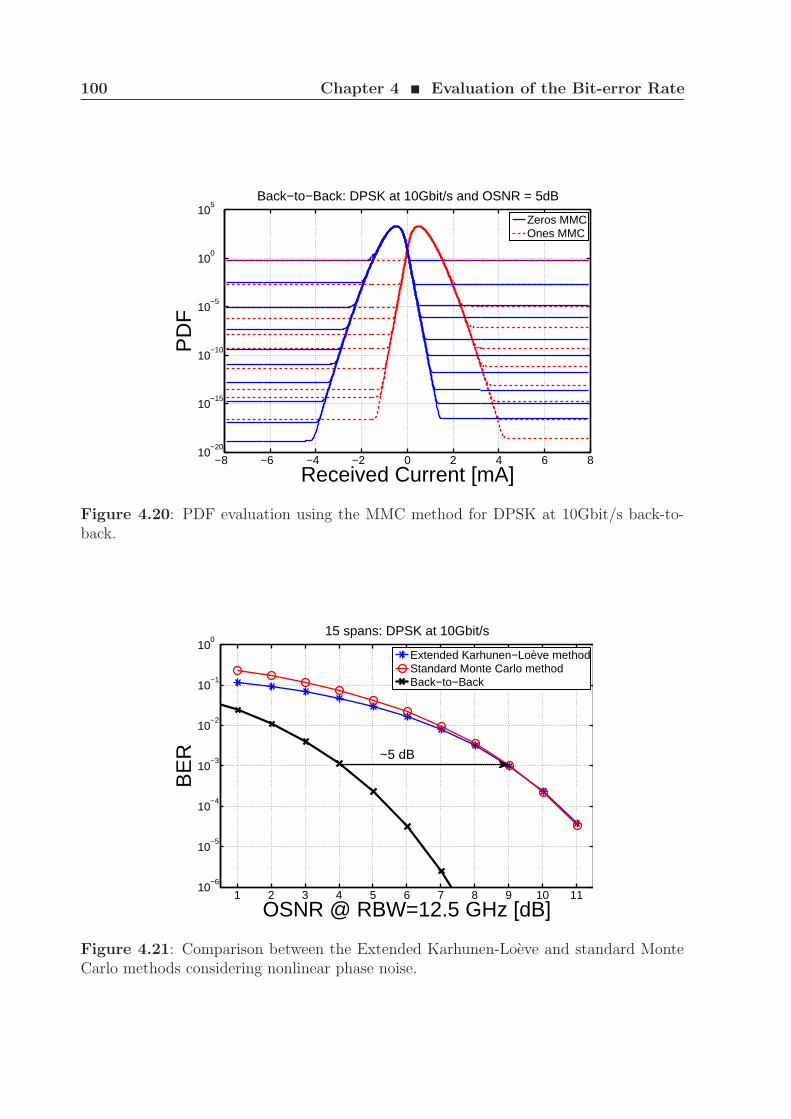
100 Chapter 4 ¥ Evaluation of the Bit-error Rate
−8 −6 −4 −2 0 2 4 6 810
−20
10−15
10−10
10−5
100
105
Received Current [mA]
PD
FBack−to−Back: DPSK at 10Gbit/s and OSNR = 5dB
Zeros MMCOnes MMC
Figure 4.20: PDF evaluation using the MMC method for DPSK at 10Gbit/s back-to-back.
1 2 3 4 5 6 7 8 9 10 1110
−6
10−5
10−4
10−3
10−2
10−1
100
OSNR @ RBW=12.5 GHz [dB]
BE
R
15 spans: DPSK at 10Gbit/s
Extended Karhunen−Loève methodStandard Monte Carlo methodBack−to−Back
~5 dB
Figure 4.21: Comparison between the Extended Karhunen-Loeve and standard MonteCarlo methods considering nonlinear phase noise.
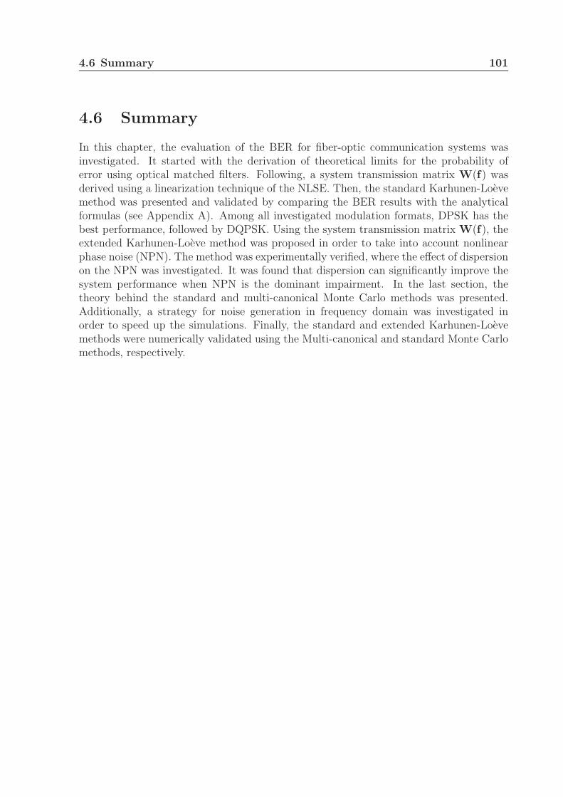
4.6 Summary 101
4.6 Summary
In this chapter, the evaluation of the BER for fiber-optic communication systems wasinvestigated. It started with the derivation of theoretical limits for the probability oferror using optical matched filters. Following, a system transmission matrix W(f) wasderived using a linearization technique of the NLSE. Then, the standard Karhunen-Loevemethod was presented and validated by comparing the BER results with the analyticalformulas (see Appendix A). Among all investigated modulation formats, DPSK has thebest performance, followed by DQPSK. Using the system transmission matrix W(f), theextended Karhunen-Loeve method was proposed in order to take into account nonlinearphase noise (NPN). The method was experimentally verified, where the effect of dispersionon the NPN was investigated. It was found that dispersion can significantly improve thesystem performance when NPN is the dominant impairment. In the last section, thetheory behind the standard and multi-canonical Monte Carlo methods was presented.Additionally, a strategy for noise generation in frequency domain was investigated inorder to speed up the simulations. Finally, the standard and extended Karhunen-Loevemethods were numerically validated using the Multi-canonical and standard Monte Carlomethods, respectively.
5Long-Haul OpticalTransmission Systems
Long-haul fiber-optic communication systems are designed to transmit information overdistances between 100 and 10.000 km. They can be divided into two main categories: ter-restrial and submarine systems. While submarine systems are designed on a customizedbasis, terrestrial systems should be flexible and relatively simple in order to adapt toexisting and future optical networks. In this thesis, only terrestrial systems will be inves-tigated, although most of the results can be applied to certain submarine systems.
The transmission of an optical signal over long distances requires periodic optical am-plification, even if low-loss fibers are used. This task is performed by EDFA’s. After eachamplifier, ASE noise is added to the amplified signal, which periodically decreases theoptical signal-to-noise ratio (OSNR). Additionally to amplification, chromatic dispersionshould be compensated for data rates equal to or above 10 Gbit/s. Since dispersion is alinear effect, it can be compensated by simply using another fiber, which generates thesame amount of chromatic dispersion, but with an opposite sign. This type of fiber isknown as dispersion-compensating fiber (DCF) and is usually employed together with op-tical amplifiers in a discrete module. The standard single-mode fiber (SMF) is the mostcommon transmission fiber. One section is normally 80 km long, according to the ITU-Trecommendation for terrestrial networks [Rec98]. The loss in optical fibers varies withthe wavelength and has its minimum around 1.55µm, which fortunately overlaps with theoperation window of an EDFA.
The transmission bandwidth is basically limited by the amplifier bandwidth, which isapproximately 40 nm ≈ 5.000 GHz at 1.55µm for an EDFA. The modulation of the wholebandwidth is not possible due to the response limitation of the available optical and electri-
5.1 Link Design 103
cal components. One solution to this problem that has been very successful is wavelengthdivision multiplex (WDM), where the information is distributed over several wavelengthsand independently transmitted. A special feature of WDM systems is that the discretewavelengths form an set of carriers which can be separated, routed, and switched withoutinterfering with one another, as long as linear crosstalk and nonlinear effects are keptlow [Kei99]. The ITU-T Recommendation G.692 [Rec98] specifies selecting the chan-nels from a grid of frequencies referenced to 193.1 THz and spacing them 50 GHz (denseWDM), 100 GHz (WDM) and 200 GHz (coarse WDM) apart.
The performance of WDM systems is evaluated by solving the coupled NLSE (2.65) forseveral channels propagating through a link. In practical systems, additionally to randombirefringence and ASE noise, the carrier phase and polarization state of each channelat the transmitter are also random variables. Since the impact of nonlinear inter- andintra-channel fiber effects depends on these random variables, the performance evaluationof WDM systems can be very time consuming, specially if one or more parameters areoptimized. Significant computational time can be saved if only one channel is simulated.In fact, the impact of the neighboring channels was shown to be less than 3 dB penalty inOSNR for OOK systems [CHH+01, HEG+04]. Therefore, single-channel simulation canoften give a very good estimation of the overall system performance in a feasible com-putational time. In the following sections, single-channel long-haul optical transmissionsystems are described and investigated.
5.1 Link Design
As already mentioned, the accumulated dispersion after LSMF = 80 km of SMF fiber canbe compensated using DCF fiber of length
LDCF =dres − DSMF · LSMF
DDCF
, (5.1)
where
DSMF = −2πcβSMF2
λ0
DDCF = −2πcβDCF2
λ0
are the dispersion per unit length parameter of the respective fibers, dres is the residualdispersion per span and L is the length of the respective fibers. For a system operatingin the linear regime, the best system performance occurs when the chromatic dispersionis fully compensated (dres = 0). If fiber nonlinearities are of concern, then the bestperformance may not be at full dispersion compensation (dres 6= 0). Therefore, the locationand length of the DCF fibers strongly affects the transmission performance and it isdefined as the dispersion map. The best dispersion map for a given system configurationand power regime can be found through optimization.
Fig. 5.1(a) shows a typical long-haul fiber-optic communication system comprising Nidentically equipped transmission sections, here defined as spans. The link is composed ofa fiber for pre-compensation, SMF and DCF fibers for in-line dispersion compensation, afiber for post-compensation and optical amplifiers with equal noise figure Fn = 6 dB. PTX,
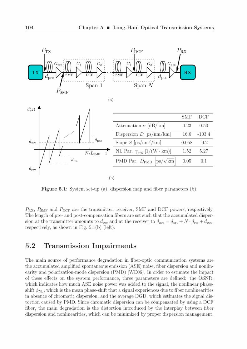
104 Chapter 5 ¥ Long-Haul Optical Transmission Systems
RXTX SMF DCF SMF DCF
G1 G2 G1 G2
PDCF
Span NPSMF
Span 1
dpre dpos
PRX
Gpre Gpos
PTX
(a)
dres
dacc
dpre
N ·LSMF
d(z)
dpos
z
SMF DCF
Attenuation α [dB/km] 0.23 0.50
Dispersion D [ps/nm/km] 16.6 -103.4
Slope S [ps/nm2/km] 0.058 -0.2
NL Par. γavg [1/(W · km)] 1.52 5.27
PMD Par. DPMD
[ps/
√km
]0.05 0.1
(b)
Figure 5.1: System set-up (a), dispersion map and fiber parameters (b).
PRX, PSMF and PDCF are the transmitter, receiver, SMF and DCF powers, respectively.The length of pre- and post-compensation fibers are set such that the accumulated disper-sion at the transmitter amounts to dpre and at the receiver to dacc = dpre + N · dres + dpos,respectively, as shown in Fig. 5.1(b) (left).
5.2 Transmission Impairments
The main source of performance degradation in fiber-optic communication systems arethe accumulated amplified spontaneous emission (ASE) noise, fiber dispersion and nonlin-earity and polarization-mode dispersion (PMD) [WE06]. In order to estimate the impactof these effects on the system performance, three parameters are defined: the OSNR,which indicates how much ASE noise power was added to the signal, the nonlinear phase-shift φNL, which is the mean phase-shift that a signal experiences due to fiber nonlinearitiesin absence of chromatic dispersion, and the average DGD, which estimates the signal dis-tortion caused by PMD. Since chromatic dispersion can be compensated by using a DCFfiber, the main degradation is the distortion introduced by the interplay between fiberdispersion and nonlinearities, which can be minimized by proper dispersion management.
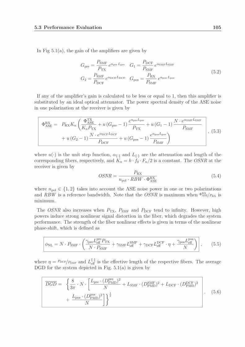
5.3 Performance Evaluation 105
In Fig 5.1(a), the gain of the amplifiers are given by
Gpre =PSMF
PTX
eαpre Lpre G1 =PDCF
PSMF
eαSMFLSMF
G2 =PSMF
PDCF
eαDCFLDCF Gpos =PRX
PSMF
eαpos Lpos
(5.2)
If any of the amplifier’s gain is calculated to be less or equal to 1, then this amplifier issubstituted by an ideal optical attenuator. The power spectral density of the ASE noisein one polarization at the receiver is given by
ΦRXASE = PRXKn
(ΦTX
ASE
KnPTX
+ u (Gpre − 1)eαpreLpre
PTX
+ u (G1 − 1)N · eαSMFLSMF
PSMF
+ u (G2 − 1)N · eαDCFLDCF
PDCF
+ u (Gpos − 1)eαposLpos
PSMF
) , (5.3)
where u(·) is the unit step function, α· and L· are the attenuation and length of thecorresponding fibers, respectively, and Kn = h · f0 ·Fn/2 is a constant. The OSNR at thereceiver is given by
OSNR =PRX
npol · RBW · ΦRXASE
(5.4)
where npol ∈ 1, 2 takes into account the ASE noise power in one or two polarizationsand RBW is a reference bandwidth. Note that the OSNR is maximum when ΦRX
ASE/PRX isminimum.
The OSNR also increases when PTX, PSMF and PDCF tend to infinity. However, highpowers induce strong nonlinear signal distortion in the fiber, which degrades the systemperformance. The strength of the fiber nonlinear effects is given in terms of the nonlinearphase-shift, which is defined as
φNL = N · PSMF ·(
γpreLpreeff PTX
N · PSMF
+ γSMFLSMFeff + γDCFLDCF
eff · η +γposL
poseff
N
), (5.5)
where η = PDCF/PSMF and L·eff is the effective length of the respective fibers. The average
DGD for the system depicted in Fig. 5.1(a) is given by
DGD =
8
3π· N ·
[Lpre · (Dpre
PMD)2
N+ LSMF · (DSMF
PMD)2 + LDCF · (DDCFPMD)2
+Lpos · (Dpos
PMD)2
N
] 12
. (5.6)
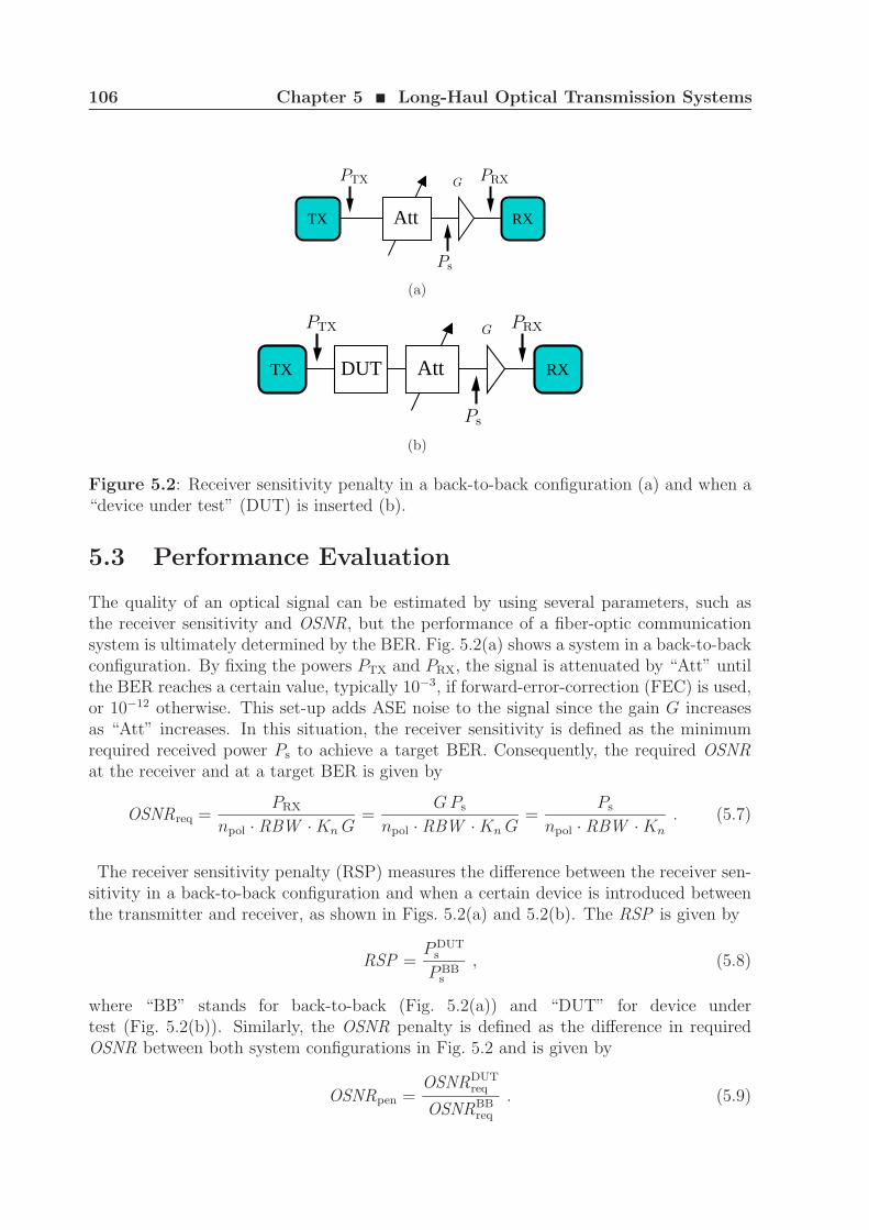
106 Chapter 5 ¥ Long-Haul Optical Transmission Systems
AttTX RX
GPTX PRX
Ps
(a)
AttDUT RXTX
GPTX PRX
Ps
(b)
Figure 5.2: Receiver sensitivity penalty in a back-to-back configuration (a) and when a“device under test” (DUT) is inserted (b).
5.3 Performance Evaluation
The quality of an optical signal can be estimated by using several parameters, such asthe receiver sensitivity and OSNR, but the performance of a fiber-optic communicationsystem is ultimately determined by the BER. Fig. 5.2(a) shows a system in a back-to-backconfiguration. By fixing the powers PTX and PRX, the signal is attenuated by “Att” untilthe BER reaches a certain value, typically 10−3, if forward-error-correction (FEC) is used,or 10−12 otherwise. This set-up adds ASE noise to the signal since the gain G increasesas “Att” increases. In this situation, the receiver sensitivity is defined as the minimumrequired received power Ps to achieve a target BER. Consequently, the required OSNRat the receiver and at a target BER is given by
OSNRreq =PRX
npol · RBW · Kn G=
GPs
npol · RBW · Kn G=
Ps
npol · RBW · Kn
. (5.7)
The receiver sensitivity penalty (RSP) measures the difference between the receiver sen-sitivity in a back-to-back configuration and when a certain device is introduced betweenthe transmitter and receiver, as shown in Figs. 5.2(a) and 5.2(b). The RSP is given by
RSP =PDUT
s
PBBs
, (5.8)
where “BB” stands for back-to-back (Fig. 5.2(a)) and “DUT” for device undertest (Fig. 5.2(b)). Similarly, the OSNR penalty is defined as the difference in requiredOSNR between both system configurations in Fig. 5.2 and is given by
OSNRpen =OSNRDUT
req
OSNRBBreq
. (5.9)
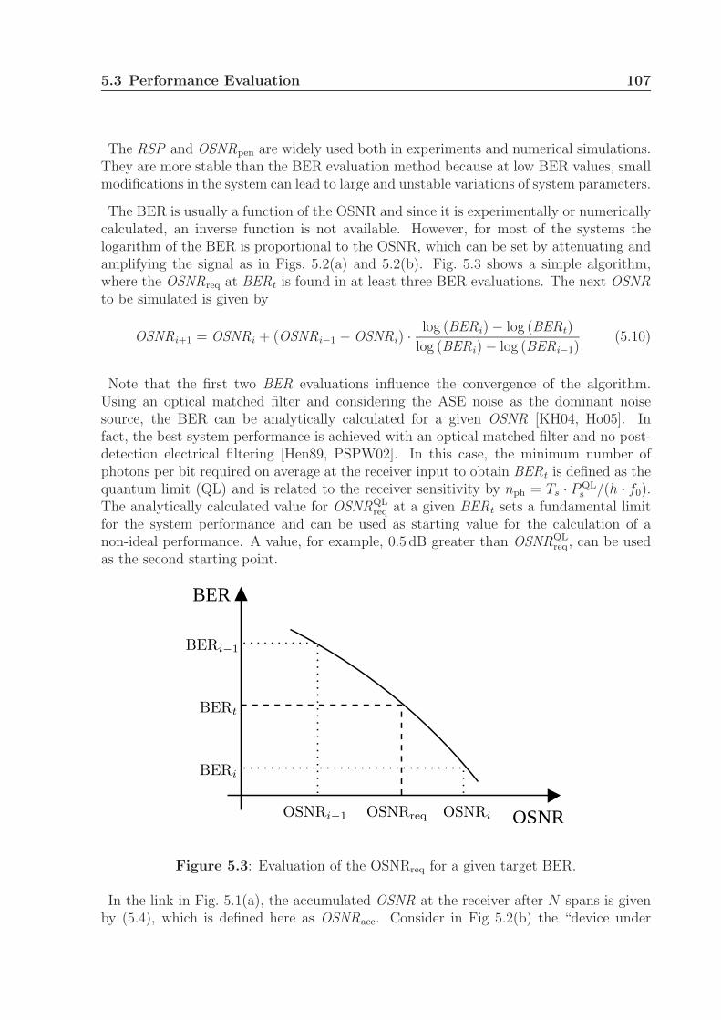
5.3 Performance Evaluation 107
The RSP and OSNRpen are widely used both in experiments and numerical simulations.They are more stable than the BER evaluation method because at low BER values, smallmodifications in the system can lead to large and unstable variations of system parameters.
The BER is usually a function of the OSNR and since it is experimentally or numericallycalculated, an inverse function is not available. However, for most of the systems thelogarithm of the BER is proportional to the OSNR, which can be set by attenuating andamplifying the signal as in Figs. 5.2(a) and 5.2(b). Fig. 5.3 shows a simple algorithm,where the OSNRreq at BERt is found in at least three BER evaluations. The next OSNRto be simulated is given by
OSNRi+1 = OSNRi + (OSNRi−1 − OSNRi) ·log (BERi) − log (BERt)
log (BERi) − log (BERi−1)(5.10)
Note that the first two BER evaluations influence the convergence of the algorithm.Using an optical matched filter and considering the ASE noise as the dominant noisesource, the BER can be analytically calculated for a given OSNR [KH04, Ho05]. Infact, the best system performance is achieved with an optical matched filter and no post-detection electrical filtering [Hen89, PSPW02]. In this case, the minimum number ofphotons per bit required on average at the receiver input to obtain BERt is defined as thequantum limit (QL) and is related to the receiver sensitivity by nph = Ts · PQL
s /(h · f0).The analytically calculated value for OSNRQL
req at a given BERt sets a fundamental limitfor the system performance and can be used as starting value for the calculation of anon-ideal performance. A value, for example, 0.5 dB greater than OSNRQL
req, can be usedas the second starting point.
BER
OSNR
BERt
OSNRi−1
BERi−1
OSNRreq OSNRi
BERi
Figure 5.3: Evaluation of the OSNRreq for a given target BER.
In the link in Fig. 5.1(a), the accumulated OSNR at the receiver after N spans is givenby (5.4), which is defined here as OSNRacc. Consider in Fig 5.2(b) the “device under
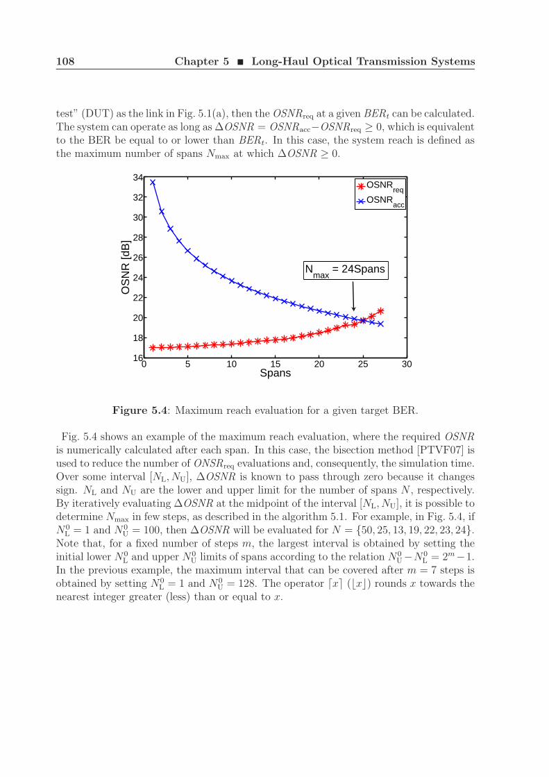
108 Chapter 5 ¥ Long-Haul Optical Transmission Systems
test” (DUT) as the link in Fig. 5.1(a), then the OSNRreq at a given BERt can be calculated.The system can operate as long as ∆OSNR = OSNRacc−OSNRreq ≥ 0, which is equivalentto the BER be equal to or lower than BERt. In this case, the system reach is defined asthe maximum number of spans Nmax at which ∆OSNR ≥ 0.
0 5 10 15 20 25 3016
18
20
22
24
26
28
30
32
34
Spans
OS
NR
[dB
]
OSNRreq
OSNRacc
Nmax
= 24Spans
Figure 5.4: Maximum reach evaluation for a given target BER.
Fig. 5.4 shows an example of the maximum reach evaluation, where the required OSNRis numerically calculated after each span. In this case, the bisection method [PTVF07] isused to reduce the number of ONSRreq evaluations and, consequently, the simulation time.Over some interval [NL, NU], ∆OSNR is known to pass through zero because it changessign. NL and NU are the lower and upper limit for the number of spans N , respectively.By iteratively evaluating ∆OSNR at the midpoint of the interval [NL, NU], it is possible todetermine Nmax in few steps, as described in the algorithm 5.1. For example, in Fig. 5.4, ifN0
L = 1 and N0U = 100, then ∆OSNR will be evaluated for N = 50, 25, 13, 19, 22, 23, 24.
Note that, for a fixed number of steps m, the largest interval is obtained by setting theinitial lower N0
L and upper N0U limits of spans according to the relation N0
U−N0L = 2m−1.
In the previous example, the maximum interval that can be covered after m = 7 steps isobtained by setting N0
L = 1 and N0U = 128. The operator ⌈x⌉ (⌊x⌋) rounds x towards the
nearest integer greater (less) than or equal to x.
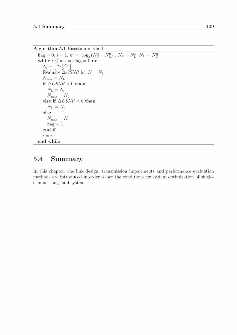
5.4 Summary 109
Algorithm 5.1 Bisection method
flag = 0, i = 1, m = ⌈log2 (N0U − N0
L)⌉, NL = N0L, NU = N0
U
while i ≤ m and flag = 0 doNi =
⌊NL+NU
2
⌋
Evaluate ∆OSNR for N = Ni
Nmax = NL
if ∆OSNR > 0 thenNL = Ni
Nmax = NL
else if ∆OSNR < 0 thenNU = Ni
elseNmax = Ni
flag = 1end ifi = i + 1
end while
5.4 Summary
In this chapter, the link design, transmission impairments and performance evaluationmethods are introduced in order to set the conditions for system optimization of single-channel long-haul systems.
6System Optimization
Over the past decades, considerable attention has been paid to the development of softwaretools that can accurately simulate and evaluate the performance of optical communicationsystems. However, the use of optimization algorithms in these softwares was restricted tosimple grid or local search methods. As optical links become more popular in communica-tion networks, the number of input parameters that can be optimized increases drastically.Due to several linear and nonlinear components, the system performance as a function ofseveral input parameters may have many local and global extrema, which is a challengefor simple optimization algorithms. Therefore, even with the large availability of powerfulcomputers or clusters, an accurate system optimization becomes a very time-consumingtask. In this context, fast optimization rules and global optimization algorithms can beemployed to guide the search over the large set of input parameters in order to find thebest solution in a minimum simulation time.
The performance of fiber-optic communication systems is usually measured in terms ofBER or OSNRreq at a target BER. Both methods require the numerical solution of thesignal propagation in the fiber and also the evaluation of the BER. Therefore, finding theoptimum fiber launch powers and dispersion map for an optical communication systemlimited by amplified spontaneous emission (ASE) noise and fiber nonlinearity is a kind ofproblem that requires a large amount of computational time.
In this Chapter, fast optimization rules and a global optimization algorithm are employedtogether with the extended Karhunen-Loeve method to find the maximum reach of single-channel DPSK and DQPSK systems including PMD and nonlinear phase noise, inducedby the interaction between the signal and ASE noise. The impact of both effects on themaximum reach is investigated for data rates ranging from 5 Gbit/s to 230 Gbit/s. First,an analytical approach based on the accumulated OSNR OSNRacc (5.4) and φNL (5.5) is
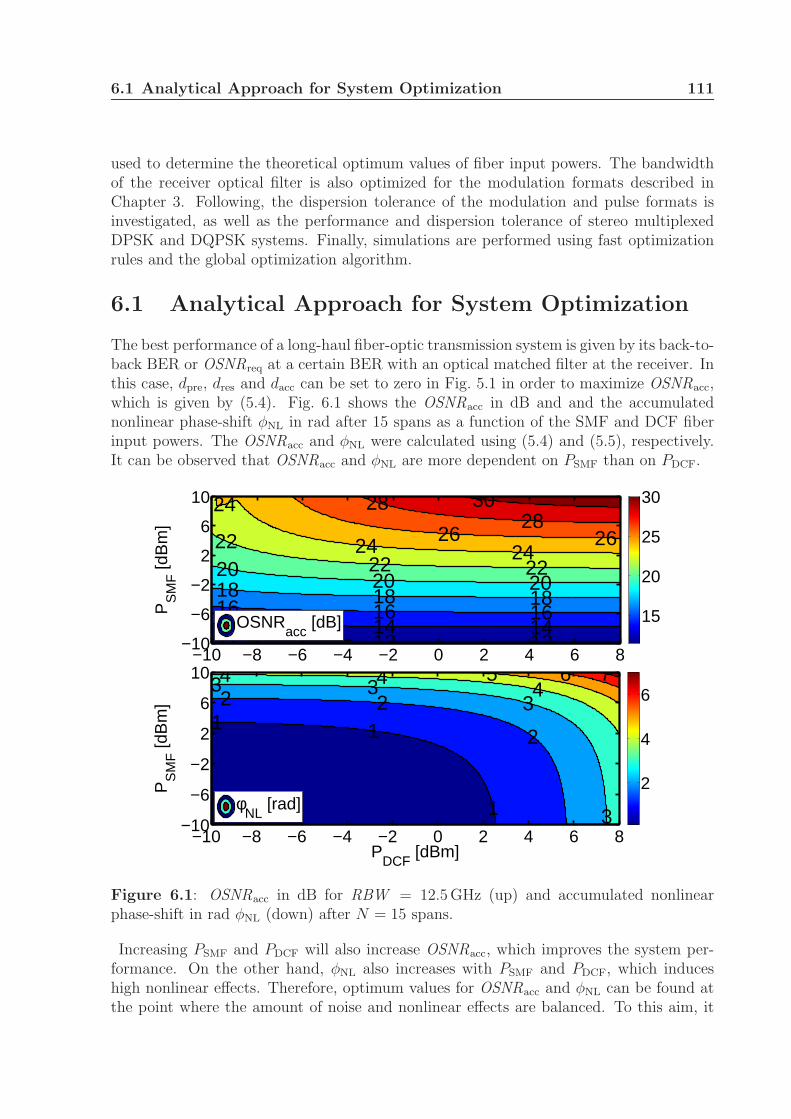
6.1 Analytical Approach for System Optimization 111
used to determine the theoretical optimum values of fiber input powers. The bandwidthof the receiver optical filter is also optimized for the modulation formats described inChapter 3. Following, the dispersion tolerance of the modulation and pulse formats isinvestigated, as well as the performance and dispersion tolerance of stereo multiplexedDPSK and DQPSK systems. Finally, simulations are performed using fast optimizationrules and the global optimization algorithm.
6.1 Analytical Approach for System Optimization
The best performance of a long-haul fiber-optic transmission system is given by its back-to-back BER or OSNRreq at a certain BER with an optical matched filter at the receiver. Inthis case, dpre, dres and dacc can be set to zero in Fig. 5.1 in order to maximize OSNRacc,which is given by (5.4). Fig. 6.1 shows the OSNRacc in dB and and the accumulatednonlinear phase-shift φNL in rad after 15 spans as a function of the SMF and DCF fiberinput powers. The OSNRacc and φNL were calculated using (5.4) and (5.5), respectively.It can be observed that OSNRacc and φNL are more dependent on PSMF than on PDCF.
121212141414 161616 181818 202020 2222
22 2424
24
262628
28 30
PS
MF [d
Bm
]
−10 −8 −6 −4 −2 0 2 4 6 8−10
−6
−2
2
6
10
15
20
25
30
OSNRacc
[dB]
1
112
22
3
333 444 5 6 7
PDCF
[dBm]
PS
MF [d
Bm
]
−10 −8 −6 −4 −2 0 2 4 6 8−10
−6
−2
2
6
10
2
4
6
φNL
[rad]
Figure 6.1: OSNRacc in dB for RBW = 12.5 GHz (up) and accumulated nonlinearphase-shift in rad φNL (down) after N = 15 spans.
Increasing PSMF and PDCF will also increase OSNRacc, which improves the system per-formance. On the other hand, φNL also increases with PSMF and PDCF, which induceshigh nonlinear effects. Therefore, optimum values for OSNRacc and φNL can be found atthe point where the amount of noise and nonlinear effects are balanced. To this aim, it
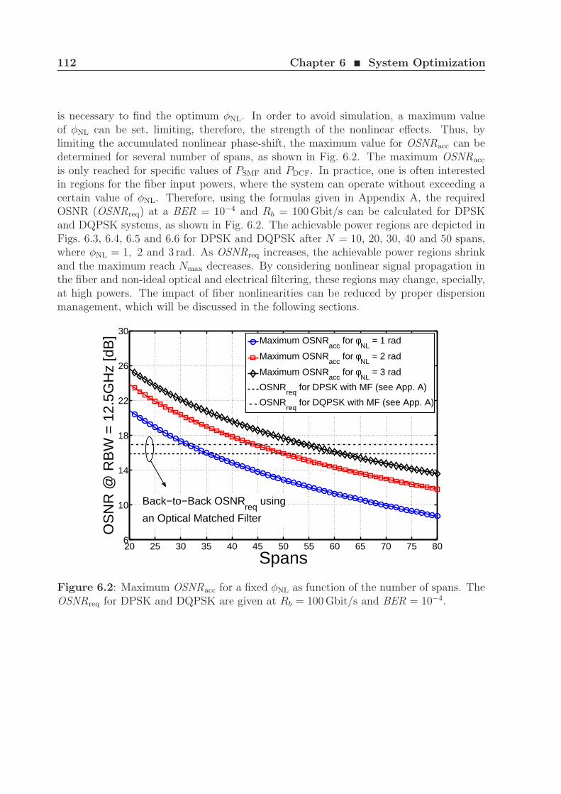
112 Chapter 6 ¥ System Optimization
is necessary to find the optimum φNL. In order to avoid simulation, a maximum valueof φNL can be set, limiting, therefore, the strength of the nonlinear effects. Thus, bylimiting the accumulated nonlinear phase-shift, the maximum value for OSNRacc can bedetermined for several number of spans, as shown in Fig. 6.2. The maximum OSNRacc
is only reached for specific values of PSMF and PDCF. In practice, one is often interestedin regions for the fiber input powers, where the system can operate without exceeding acertain value of φNL. Therefore, using the formulas given in Appendix A, the requiredOSNR (OSNRreq) at a BER = 10−4 and Rb = 100 Gbit/s can be calculated for DPSKand DQPSK systems, as shown in Fig. 6.2. The achievable power regions are depicted inFigs. 6.3, 6.4, 6.5 and 6.6 for DPSK and DQPSK after N = 10, 20, 30, 40 and 50 spans,where φNL = 1, 2 and 3 rad. As OSNRreq increases, the achievable power regions shrinkand the maximum reach Nmax decreases. By considering nonlinear signal propagation inthe fiber and non-ideal optical and electrical filtering, these regions may change, specially,at high powers. The impact of fiber nonlinearities can be reduced by proper dispersionmanagement, which will be discussed in the following sections.
20 25 30 35 40 45 50 55 60 65 70 75 806
10
14
18
22
26
30
Spans
OS
NR
@ R
BW
= 1
2.5G
Hz
[dB
]
Maximum OSNRacc
for φNL
= 1 rad
Maximum OSNRacc
for φNL
= 2 rad
Maximum OSNRacc
for φNL
= 3 rad
OSNRreq
for DPSK with MF (see App. A)
OSNRreq
for DQPSK with MF (see App. A)
Back−to−Back OSNRreq
using
an Optical Matched Filter
Figure 6.2: Maximum OSNRacc for a fixed φNL as function of the number of spans. TheOSNRreq for DPSK and DQPSK are given at Rb = 100 Gbit/s and BER = 10−4.
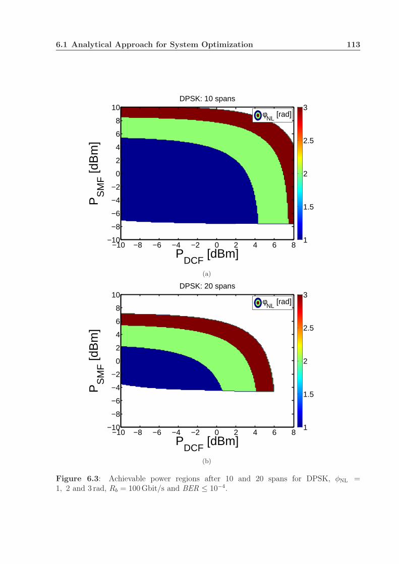
6.1 Analytical Approach for System Optimization 113
PDCF
[dBm]
PS
MF [d
Bm
]DPSK: 10 spans
−10 −8 −6 −4 −2 0 2 4 6 8−10
−8
−6
−4
−2
0
2
4
6
8
10
1
1.5
2
2.5
3φ
NL [rad]
(a)
PDCF
[dBm]
PS
MF [d
Bm
]
DPSK: 20 spans
−10 −8 −6 −4 −2 0 2 4 6 8−10
−8
−6
−4
−2
0
2
4
6
8
10
1
1.5
2
2.5
3φ
NL [rad]
(b)
Figure 6.3: Achievable power regions after 10 and 20 spans for DPSK, φNL =1, 2 and 3 rad, Rb = 100 Gbit/s and BER ≤ 10−4.
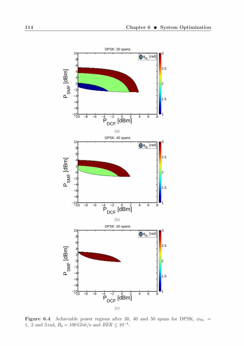
114 Chapter 6 ¥ System Optimization
PDCF
[dBm]
PS
MF [d
Bm
]
DPSK: 30 spans
−10 −8 −6 −4 −2 0 2 4 6 8−10
−8
−6
−4
−2
0
2
4
6
8
10
1
1.5
2
2.5
3φ
NL [rad]
(a)
PDCF
[dBm]
PS
MF [d
Bm
]
DPSK: 40 spans
−10 −8 −6 −4 −2 0 2 4 6 8−10
−8
−6
−4
−2
0
2
4
6
8
10
1
1.5
2
2.5
3φ
NL [rad]
(b)
PDCF
[dBm]
PS
MF [d
Bm
]
DPSK: 50 spans
−10 −8 −6 −4 −2 0 2 4 6 8−10
−8
−6
−4
−2
0
2
4
6
8
10
1
1.5
2
2.5
3φ
NL [rad]
(c)
Figure 6.4: Achievable power regions after 30, 40 and 50 spans for DPSK, φNL =1, 2 and 3 rad, Rb = 100 Gbit/s and BER ≤ 10−4.

6.1 Analytical Approach for System Optimization 115
PDCF
[dBm]
PS
MF [d
Bm
]DQPSK: 10 spans
−10 −8 −6 −4 −2 0 2 4 6 8−10
−8
−6
−4
−2
0
2
4
6
8
10
1
1.5
2
2.5
3φ
NL [rad]
(a)
PDCF
[dBm]
PS
MF [d
Bm
]
DQPSK: 20 spans
−10 −8 −6 −4 −2 0 2 4 6 8−10
−8
−6
−4
−2
0
2
4
6
8
10
1
1.5
2
2.5
3φ
NL [rad]
(b)
Figure 6.5: Achievable power regions after 10 and 20 spans for DQPSK, φNL =1, 2 and 3 rad, Rb = 100 Gbit/s and BER ≤ 10−4.
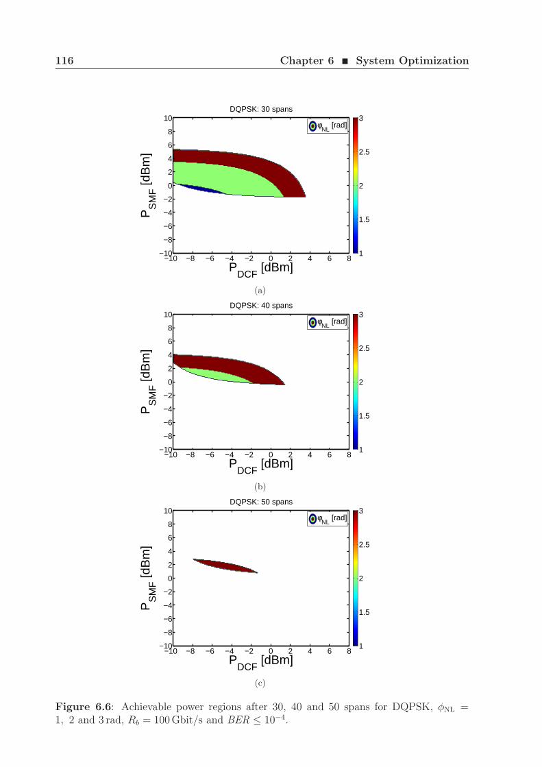
116 Chapter 6 ¥ System Optimization
PDCF
[dBm]
PS
MF [d
Bm
]
DQPSK: 30 spans
−10 −8 −6 −4 −2 0 2 4 6 8−10
−8
−6
−4
−2
0
2
4
6
8
10
1
1.5
2
2.5
3φ
NL [rad]
(a)
PDCF
[dBm]
PS
MF [d
Bm
]
DQPSK: 40 spans
−10 −8 −6 −4 −2 0 2 4 6 8−10
−8
−6
−4
−2
0
2
4
6
8
10
1
1.5
2
2.5
3φ
NL [rad]
(b)
PDCF
[dBm]
PS
MF [d
Bm
]
DQPSK: 50 spans
−10 −8 −6 −4 −2 0 2 4 6 8−10
−8
−6
−4
−2
0
2
4
6
8
10
1
1.5
2
2.5
3φ
NL [rad]
(c)
Figure 6.6: Achievable power regions after 30, 40 and 50 spans for DQPSK, φNL =1, 2 and 3 rad, Rb = 100 Gbit/s and BER ≤ 10−4.
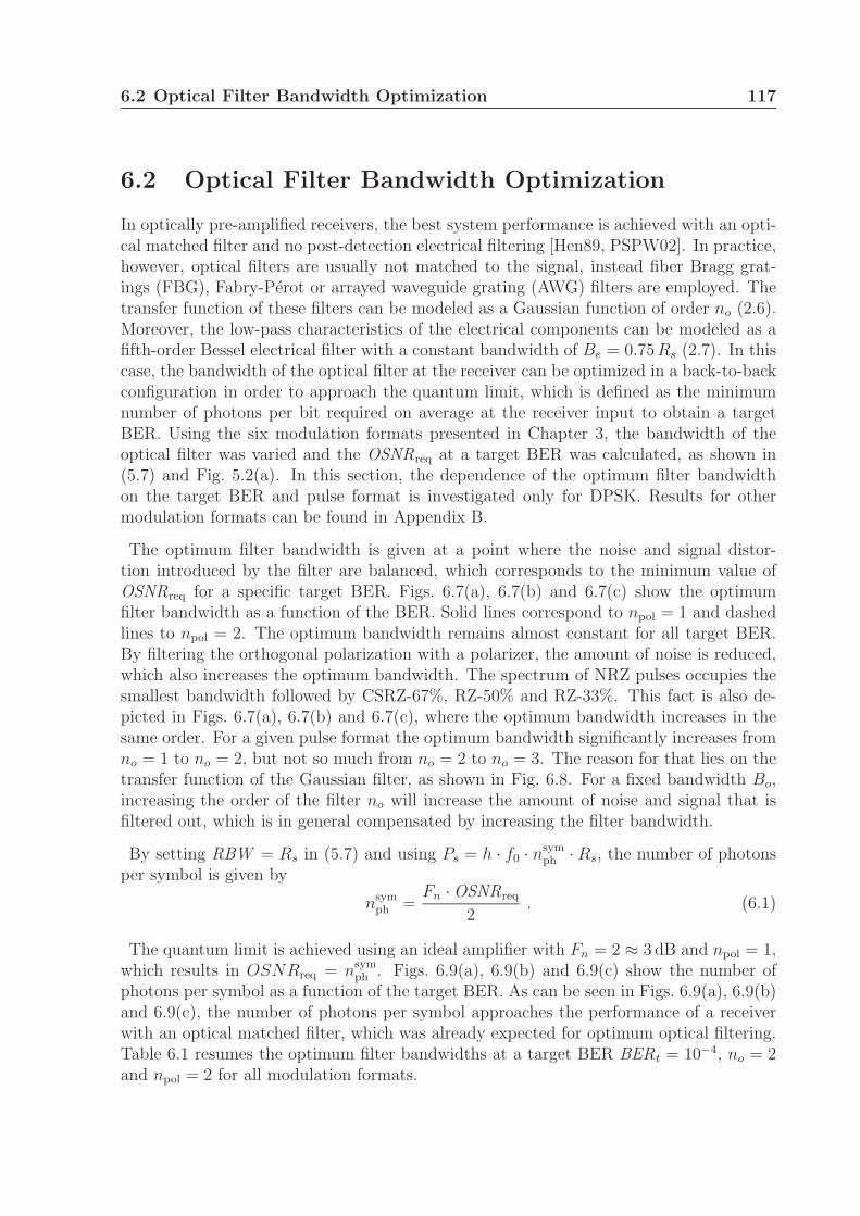
6.2 Optical Filter Bandwidth Optimization 117
6.2 Optical Filter Bandwidth Optimization
In optically pre-amplified receivers, the best system performance is achieved with an opti-cal matched filter and no post-detection electrical filtering [Hen89, PSPW02]. In practice,however, optical filters are usually not matched to the signal, instead fiber Bragg grat-ings (FBG), Fabry-Perot or arrayed waveguide grating (AWG) filters are employed. Thetransfer function of these filters can be modeled as a Gaussian function of order no (2.6).Moreover, the low-pass characteristics of the electrical components can be modeled as afifth-order Bessel electrical filter with a constant bandwidth of Be = 0.75 Rs (2.7). In thiscase, the bandwidth of the optical filter at the receiver can be optimized in a back-to-backconfiguration in order to approach the quantum limit, which is defined as the minimumnumber of photons per bit required on average at the receiver input to obtain a targetBER. Using the six modulation formats presented in Chapter 3, the bandwidth of theoptical filter was varied and the OSNRreq at a target BER was calculated, as shown in(5.7) and Fig. 5.2(a). In this section, the dependence of the optimum filter bandwidthon the target BER and pulse format is investigated only for DPSK. Results for othermodulation formats can be found in Appendix B.
The optimum filter bandwidth is given at a point where the noise and signal distor-tion introduced by the filter are balanced, which corresponds to the minimum value ofOSNRreq for a specific target BER. Figs. 6.7(a), 6.7(b) and 6.7(c) show the optimumfilter bandwidth as a function of the BER. Solid lines correspond to npol = 1 and dashedlines to npol = 2. The optimum bandwidth remains almost constant for all target BER.By filtering the orthogonal polarization with a polarizer, the amount of noise is reduced,which also increases the optimum bandwidth. The spectrum of NRZ pulses occupies thesmallest bandwidth followed by CSRZ-67%, RZ-50% and RZ-33%. This fact is also de-picted in Figs. 6.7(a), 6.7(b) and 6.7(c), where the optimum bandwidth increases in thesame order. For a given pulse format the optimum bandwidth significantly increases fromno = 1 to no = 2, but not so much from no = 2 to no = 3. The reason for that lies on thetransfer function of the Gaussian filter, as shown in Fig. 6.8. For a fixed bandwidth Bo,increasing the order of the filter no will increase the amount of noise and signal that isfiltered out, which is in general compensated by increasing the filter bandwidth.
By setting RBW = Rs in (5.7) and using Ps = h · f0 · nsymph · Rs, the number of photons
per symbol is given by
nsymph =
Fn · OSNRreq
2. (6.1)
The quantum limit is achieved using an ideal amplifier with Fn = 2 ≈ 3 dB and npol = 1,which results in OSNRreq = nsym
ph . Figs. 6.9(a), 6.9(b) and 6.9(c) show the number ofphotons per symbol as a function of the target BER. As can be seen in Figs. 6.9(a), 6.9(b)and 6.9(c), the number of photons per symbol approaches the performance of a receiverwith an optical matched filter, which was already expected for optimum optical filtering.Table 6.1 resumes the optimum filter bandwidths at a target BER BERt = 10−4, no = 2and npol = 2 for all modulation formats.
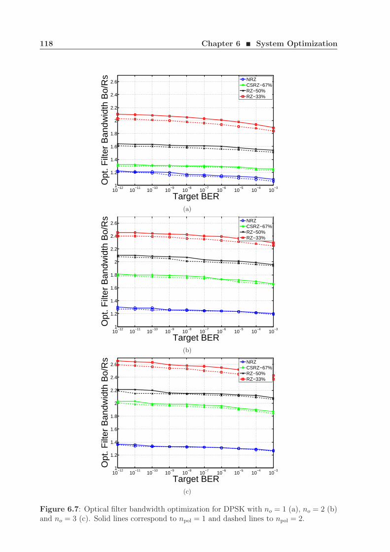
118 Chapter 6 ¥ System Optimization
10−12
10−11
10−10
10−9
10−8
10−7
10−6
10−5
10−4
10−31
1.2
1.4
1.6
1.8
2
2.2
2.4
2.6
Target BER
Opt
. Filt
er B
andw
idth
Bo/
Rs
NRZCSRZ−67%RZ−50%RZ−33%
(a)
10−12
10−11
10−10
10−9
10−8
10−7
10−6
10−5
10−4
10−31
1.2
1.4
1.6
1.8
2
2.2
2.4
2.6
Target BER
Opt
. Filt
er B
andw
idth
Bo/
Rs
NRZCSRZ−67%RZ−50%RZ−33%
(b)
10−12
10−11
10−10
10−9
10−8
10−7
10−6
10−5
10−4
10−31
1.2
1.4
1.6
1.8
2
2.2
2.4
2.6
Target BER
Opt
. Filt
er B
andw
idth
Bo/
Rs
NRZCSRZ−67%RZ−50%RZ−33%
(c)
Figure 6.7: Optical filter bandwidth optimization for DPSK with no = 1 (a), no = 2 (b)and no = 3 (c). Solid lines correspond to npol = 1 and dashed lines to npol = 2.
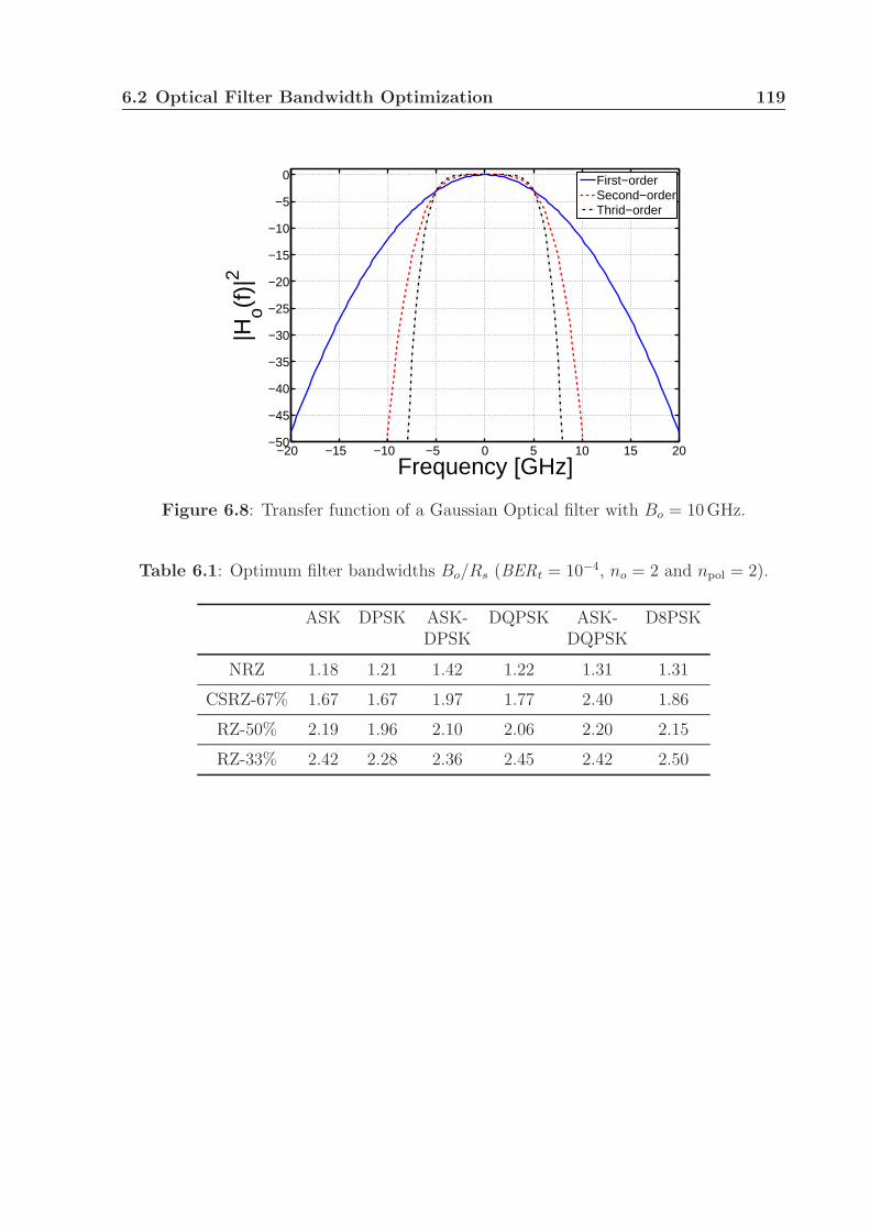
6.2 Optical Filter Bandwidth Optimization 119
−20 −15 −10 −5 0 5 10 15 20−50
−45
−40
−35
−30
−25
−20
−15
−10
−5
0
Frequency [GHz]
|Ho(f
)|2
First−orderSecond−orderThrid−order
Figure 6.8: Transfer function of a Gaussian Optical filter with Bo = 10 GHz.
Table 6.1: Optimum filter bandwidths Bo/Rs (BERt = 10−4, no = 2 and npol = 2).
ASK DPSK ASK- DQPSK ASK- D8PSKDPSK DQPSK
NRZ 1.18 1.21 1.42 1.22 1.31 1.31
CSRZ-67% 1.67 1.67 1.97 1.77 2.40 1.86
RZ-50% 2.19 1.96 2.10 2.06 2.20 2.15
RZ-33% 2.42 2.28 2.36 2.45 2.42 2.50
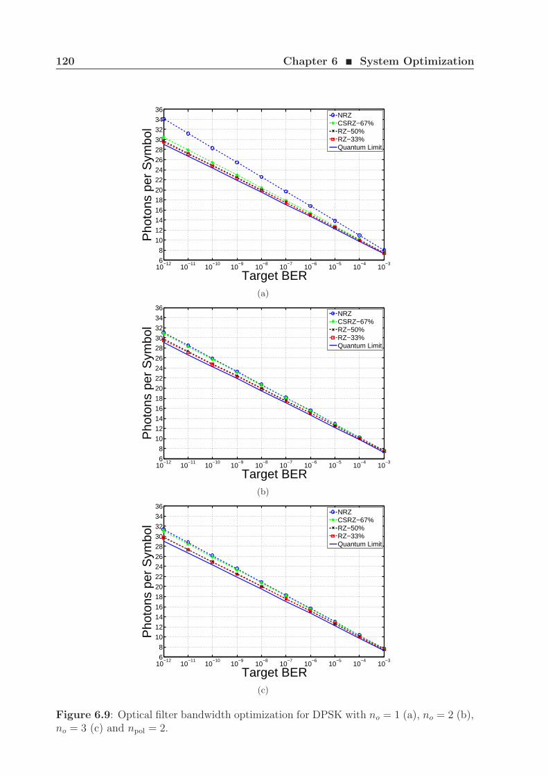
120 Chapter 6 ¥ System Optimization
10−12
10−11
10−10
10−9
10−8
10−7
10−6
10−5
10−4
10−36
8
10
12
14
16
18
20
22
24
26
28
30
32
34
36
Target BER
Pho
tons
per
Sym
bol
NRZCSRZ−67%RZ−50%RZ−33%Quantum Limit
(a)
10−12
10−11
10−10
10−9
10−8
10−7
10−6
10−5
10−4
10−36
8
10
12
14
16
18
20
22
24
26
28
30
32
34
36
Target BER
Pho
tons
per
Sym
bol
NRZCSRZ−67%RZ−50%RZ−33%Quantum Limit
(b)
10−12
10−11
10−10
10−9
10−8
10−7
10−6
10−5
10−4
10−36
8
10
12
14
16
18
20
22
24
26
28
30
32
34
36
Target BER
Pho
tons
per
Sym
bol
NRZCSRZ−67%RZ−50%RZ−33%Quantum Limit
(c)
Figure 6.9: Optical filter bandwidth optimization for DPSK with no = 1 (a), no = 2 (b),no = 3 (c) and npol = 2.
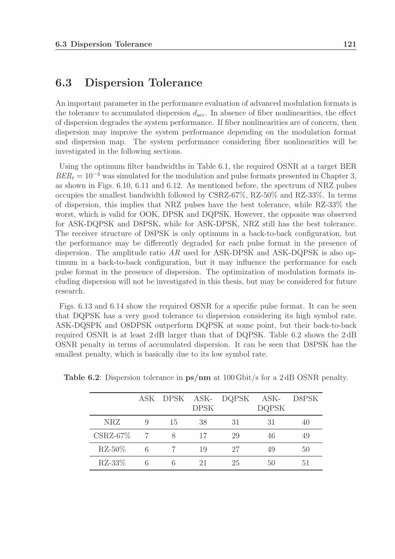
6.3 Dispersion Tolerance 121
6.3 Dispersion Tolerance
An important parameter in the performance evaluation of advanced modulation formats isthe tolerance to accumulated dispersion dacc. In absence of fiber nonlinearities, the effectof dispersion degrades the system performance. If fiber nonlinearities are of concern, thendispersion may improve the system performance depending on the modulation formatand dispersion map. The system performance considering fiber nonlinearities will beinvestigated in the following sections.
Using the optimum filter bandwidths in Table 6.1, the required OSNR at a target BERBERt = 10−4 was simulated for the modulation and pulse formats presented in Chapter 3,as shown in Figs. 6.10, 6.11 and 6.12. As mentioned before, the spectrum of NRZ pulsesoccupies the smallest bandwidth followed by CSRZ-67%, RZ-50% and RZ-33%. In termsof dispersion, this implies that NRZ pulses have the best tolerance, while RZ-33% theworst, which is valid for OOK, DPSK and DQPSK. However, the opposite was observedfor ASK-DQPSK and D8PSK, while for ASK-DPSK, NRZ still has the best tolerance.The receiver structure of D8PSK is only optimum in a back-to-back configuration, butthe performance may be differently degraded for each pulse format in the presence ofdispersion. The amplitude ratio AR used for ASK-DPSK and ASK-DQPSK is also op-timum in a back-to-back configuration, but it may influence the performance for eachpulse format in the presence of dispersion. The optimization of modulation formats in-cluding dispersion will not be investigated in this thesis, but may be considered for futureresearch.
Figs. 6.13 and 6.14 show the required OSNR for a specific pulse format. It can be seenthat DQPSK has a very good tolerance to dispersion considering its high symbol rate.ASK-DQSPK and O8DPSK outperform DQPSK at some point, but their back-to-backrequired OSNR is at least 2 dB larger than that of DQPSK. Table 6.2 shows the 2 dBOSNR penalty in terms of accumulated dispersion. It can be seen that D8PSK has thesmallest penalty, which is basically due to its low symbol rate.
Table 6.2: Dispersion tolerance in ps/nm at 100 Gbit/s for a 2 dB OSNR penalty.
ASK DPSK ASK- DQPSK ASK- D8PSKDPSK DQPSK
NRZ 9 15 38 31 31 40
CSRZ-67% 7 8 17 29 46 49
RZ-50% 6 7 19 27 49 50
RZ-33% 6 6 21 25 50 51
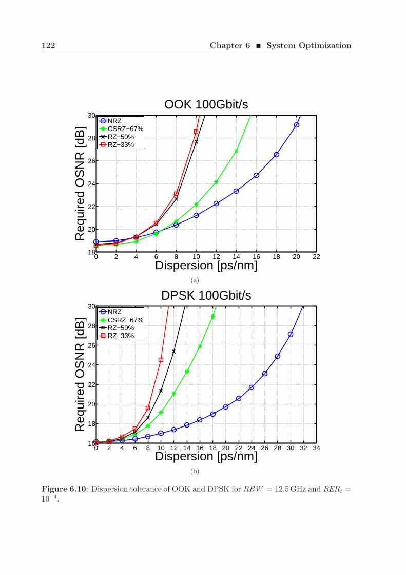
122 Chapter 6 ¥ System Optimization
0 2 4 6 8 10 12 14 16 18 20 2218
20
22
24
26
28
30
Dispersion [ps/nm]
Req
uire
d O
SN
R [d
B]
OOK 100Gbit/s
NRZCSRZ−67%RZ−50%RZ−33%
(a)
0 2 4 6 8 10 12 14 16 18 20 22 24 26 28 30 32 3416
18
20
22
24
26
28
30
Dispersion [ps/nm]
Req
uire
d O
SN
R [d
B]
DPSK 100Gbit/s
NRZCSRZ−67%RZ−50%RZ−33%
(b)
Figure 6.10: Dispersion tolerance of OOK and DPSK for RBW = 12.5 GHz and BERt =10−4.
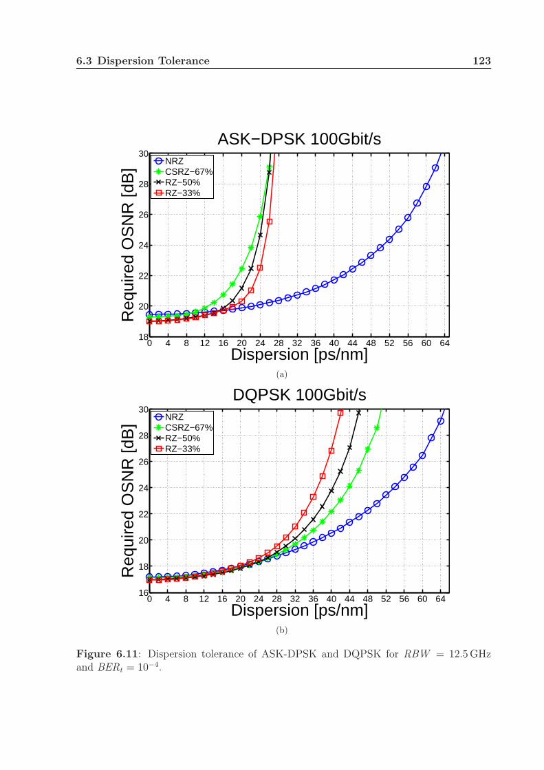
6.3 Dispersion Tolerance 123
0 4 8 12 16 20 24 28 32 36 40 44 48 52 56 60 6418
20
22
24
26
28
30
Dispersion [ps/nm]
Req
uire
d O
SN
R [d
B]
ASK−DPSK 100Gbit/s
NRZCSRZ−67%RZ−50%RZ−33%
(a)
0 4 8 12 16 20 24 28 32 36 40 44 48 52 56 60 6416
18
20
22
24
26
28
30
Dispersion [ps/nm]
Req
uire
d O
SN
R [d
B]
DQPSK 100Gbit/s
NRZCSRZ−67%RZ−50%RZ−33%
(b)
Figure 6.11: Dispersion tolerance of ASK-DPSK and DQPSK for RBW = 12.5 GHzand BERt = 10−4.

124 Chapter 6 ¥ System Optimization
0 4 8 12 16 20 24 28 32 36 40 44 48 52 56 60 64 68 7218
20
22
24
26
28
30
Dispersion [ps/nm]
Req
uire
d O
SN
R [d
B]
ASK−DQPSK 100Gbit/s
NRZCSRZ−67%RZ−50%RZ−33%
(a)
0 4 8 12 16 20 24 28 32 36 40 44 48 52 56 60 64 68 72 76 8020
22
24
26
28
30
Dispersion [ps/nm]
Req
uire
d O
SN
R [d
B]
OD8PSK 100Gbit/s
NRZCSRZ−67%RZ−50%RZ−33%
(b)
Figure 6.12: Dispersion tolerance of ASK-DQPSK and D8PSK for RBW = 12.5 GHzand BERt = 10−4.
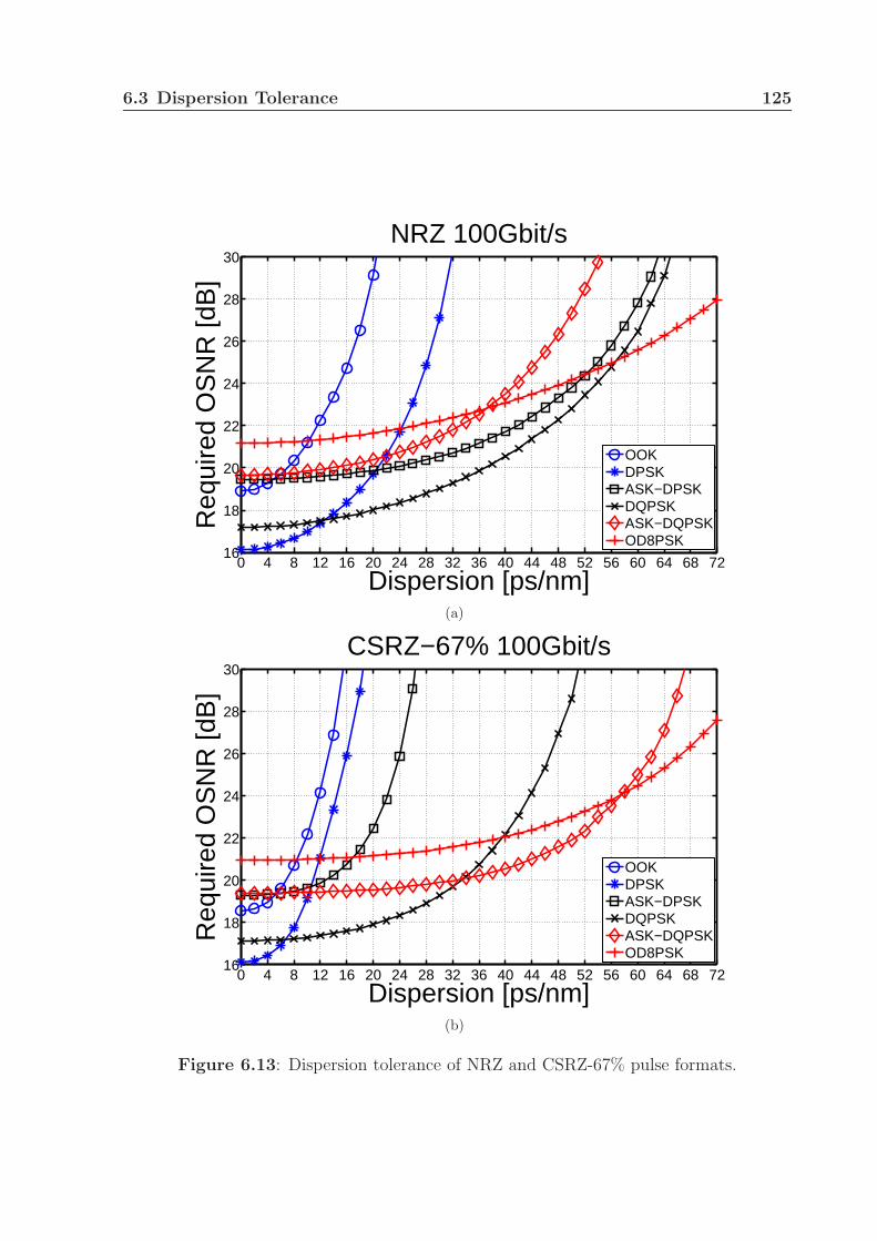
6.3 Dispersion Tolerance 125
0 4 8 12 16 20 24 28 32 36 40 44 48 52 56 60 64 68 7216
18
20
22
24
26
28
30
Dispersion [ps/nm]
Req
uire
d O
SN
R [d
B]
NRZ 100Gbit/s
OOKDPSKASK−DPSKDQPSKASK−DQPSKOD8PSK
(a)
0 4 8 12 16 20 24 28 32 36 40 44 48 52 56 60 64 68 7216
18
20
22
24
26
28
30
Dispersion [ps/nm]
Req
uire
d O
SN
R [d
B]
CSRZ−67% 100Gbit/s
OOKDPSKASK−DPSKDQPSKASK−DQPSKOD8PSK
(b)
Figure 6.13: Dispersion tolerance of NRZ and CSRZ-67% pulse formats.
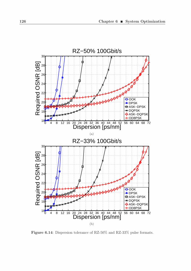
126 Chapter 6 ¥ System Optimization
0 4 8 12 16 20 24 28 32 36 40 44 48 52 56 60 64 68 7216
18
20
22
24
26
28
30
Dispersion [ps/nm]
Req
uire
d O
SN
R [d
B]
RZ−50% 100Gbit/s
OOKDPSKASK−DPSKDQPSKASK−DQPSKOD8PSK
(a)
0 4 8 12 16 20 24 28 32 36 40 44 48 52 56 60 64 68 7216
18
20
22
24
26
28
30
Dispersion [ps/nm]
Req
uire
d O
SN
R [d
B]
RZ−33% 100Gbit/s
OOKDPSKASK−DPSKDQPSKASK−DQPSKOD8PSK
(b)
Figure 6.14: Dispersion tolerance of RZ-50% and RZ-33% pulse formats.

6.3 Dispersion Tolerance 127
6.3.1 Performance of Stereo Multiplexed Systems
Stereo multiplexing allows the transmission of higher data rates using low-bandwidthcomponents, as discussed in Chapter 3. In order to evaluate the performance of DPSKand DQPSK stereo multiplexed systems, the back-to-back sensitivity, required OSNR anddispersion tolerance were calculated for Rb = 100 Gbit/s. The separation between thetwo channels was set to ∆f = 2Rs and the bandwidth of the optical filter was optimized.Table 6.3 shows the required OSNR for stereo-DPSK and stereo-DQPSK. Comparing theperformance of stereo and conventional DPSK and DQPSK, an OSNR penalty of less than1 dB was observed for CSRZ-67% and RZ-50% pulse formats, while NRZ and RZ-33%experience a penalty of 1.5-2.5 dB. Figs. 6.15 and 6.16 show the dispersion tolerance ofstereo DPSK and DQPSK, and conventional DPSK and DQPSK for comparison. Similarto the back-to-back required OSNR, the use of CSRZ-67% or RZ-50% result in dispersiontolerances similar to conventional DPSK and DQPSK, while stereo multiplexed DPSK orDQPSK with NRZ and RZ-33% pulse formats are less tolerant to dispersion.
Theoretically, the performance of a stereo multiplexed system is equal or worse thanthe corresponding conventional modulation format. Using practical optical and electricalfilters, there may be situations where stereo multiplexing outperforms the conventionalmodulation formats, as shown in Fig. 6.15(b) for dacc > 24 ps/nm. Therefore, stereo mul-tiplexing may be suitable for systems where bandwidth requirements of the componentsare of concern.
Table 6.3: Required OSNR in dB for DPSK, DQPSK, Stereo-DPSK and Stereo-DQPSK(Rb = 100 Gbit/s, RBW = 12.5 GHz, BERt = 10−4, no = 2 and npol = 2).
Stereo DPSK DPSK Stereo DPQSK DQPSK
NRZ 17.65 16.13 18.63 17.18
CSRZ-67% 16.79 16.11 17.73 17.13
RZ-50% 16.87 16.02 17.56 16.99
RZ-33% 18.48 16.02 19.00 16.95
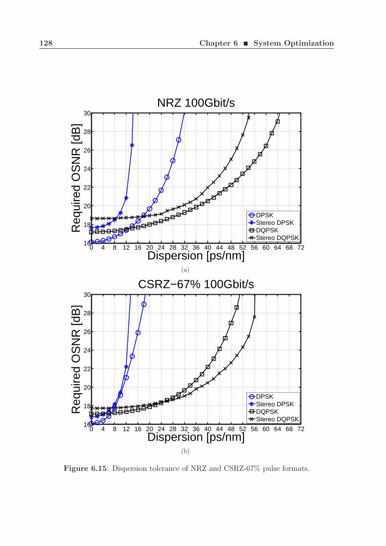
128 Chapter 6 ¥ System Optimization
0 4 8 12 16 20 24 28 32 36 40 44 48 52 56 60 64 68 7216
18
20
22
24
26
28
30
Dispersion [ps/nm]
Req
uire
d O
SN
R [d
B]
NRZ 100Gbit/s
DPSKStereo DPSKDQPSKStereo DQPSK
(a)
0 4 8 12 16 20 24 28 32 36 40 44 48 52 56 60 64 68 7216
18
20
22
24
26
28
30
Dispersion [ps/nm]
Req
uire
d O
SN
R [d
B]
CSRZ−67% 100Gbit/s
DPSKStereo DPSKDQPSKStereo DQPSK
(b)
Figure 6.15: Dispersion tolerance of NRZ and CSRZ-67% pulse formats.

6.3 Dispersion Tolerance 129
0 4 8 12 16 20 24 28 32 36 40 44 48 52 56 60 64 68 7216
18
20
22
24
26
28
30
Dispersion [ps/nm]
Req
uire
d O
SN
R [d
B]
RZ−50% 100Gbit/s
DPSKStereo DPSKDQPSKStereo DQPSK
(a)
0 4 8 12 16 20 24 28 32 36 40 44 48 52 56 60 64 68 7216
18
20
22
24
26
28
30
Dispersion [ps/nm]
Req
uire
d O
SN
R [d
B]
RZ−33% 100Gbit/s
DPSKStereo DPSKDQPSKStereo DQPSK
(b)
Figure 6.16: Dispersion tolerance of RZ-50% and RZ-33% pulse formats.

130 Chapter 6 ¥ System Optimization
6.4 Fast Optimization Rules
Neglecting the effect of PMD, the performance of long-haul fiber-optic communication sys-tems is basically limited by the accumulated ASE noise and nonlinear fiber effects. There-fore, an optimized design of fiber input powers and dispersion map is required to achievethe best system performance. This task is usually done through computer simulations,where many runs of long bit sequences are performed to account for all nonlinear effects.In this case, solving numerically the coupled or scalar nonlinear Schrodinger equation andthe evaluation of the bit-error rate can be very time-consuming. In order to simplify theoptimization process, the system performance can be estimated using the nonlinear phase-shift φNL (5.5) as a measure of the impact of nonlinear fiber effects. Figs. 4.14 and 4.15show experimental and simulation results, where the system performance depends onlyon the nonlinear phase-shift, given a fully in-line dispersion compensated scheme, with orwithout pre- and post compensation.
In this section, an optimization method for maximizing the reach of optical transmissionsystems is presented. It requires few numerical evaluations of OSNRreq and is based onthe straight-line rule [BSO08, KTMB00] and on the nonlinear phase-shift.
6.4.1 Straight-line Rule
In fiber-optic communications, the optimization of dispersion maps is a well know tech-nique, normally used to improve the system’s tolerance to nonlinear effects. In Fig. 5.1(b),the variables dpre, dres and dacc can be set such that the signal distortion after propagationthrough the link is minimized. While the optimum value of dacc basically depends on thenonlinear phase-shift φNL [BSO08, FB00], the amount of pre-compensation dpre and theresidual dispersion per span dres can be described by a linear relation, which is called herethe straight-line rule.
First, the residual dispersion per span is set to zero (dres = 0) and the DCF is consideredlinear. Using a phenomenological approach to reduce the timing jitter in 40 Gbit/s OOKsystems, Killey [KTMB00] showed that intra-channel effects arising from the nonlinearinteraction between pulses are minimized when the pulse broadening within the nonlinearlength is minimized, i.e., dpre = −DSMF · zd, where zd is given by
∫ zd
0
PSMF e−αSMF zdz =
∫ LSMF
zd
PSMFe−αSMF zdz
zd = − 1
αSMF
log
(e−αSMF LSMF + 1
2
). (6.2)
For dres 6= 0, the best performance is obtained by setting the pre-compensation such thatthe minimum width of the pulse is achieved halfway along the link length. Therefore, theamount of pre-compensation, which minimizes the intra-channel effects is given by
dpre =DSMF
αSMF
log
(e−αSMF LSMF + 1
2
)− N · dres
2. (6.3)
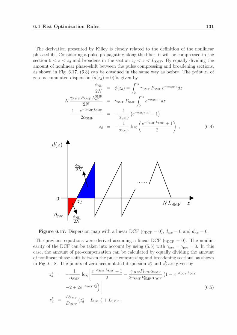
6.4 Fast Optimization Rules 131
The derivation presented by Killey is closely related to the definition of the nonlinearphase-shift. Considering a pulse propagating along the fiber, it will be compressed in thesection 0 < z < zd and broadens in the section zd < z < LSMF. By equally dividing theamount of nonlinear phase-shift between the pulse compressing and broadening sections,as shown in Fig. 6.17, (6.3) can be obtained in the same way as before. The point zd ofzero accumulated dispersion (d(zd) = 0) is given by
φNL
2N= φ(zd) =
∫ zd
0
γSMF PSMF e−αSMF zdz
NγSMF PSMF LSMF
eff
2N= γSMF PSMF
∫ zd
0
e−αSMF zdz
1 − e−αSMF LSMF
2αSMF
= − 1
αSMF
(e−αSMF zd − 1
)
zd = − 1
αSMF
log
(e−αSMF LSMF + 1
2
), (6.4)
0NLSMF
d(z)
zd
φNL
2N
dpre φNL
2N
z
Figure 6.17: Dispersion map with a linear DCF (γDCF = 0), dacc = 0 and dres = 0.
The previous equations were derived assuming a linear DCF (γDCF = 0). The nonlin-earity of the DCF can be taken into account by using (5.5) with γpre = γpos = 0. In thiscase, the amount of pre-compensation can be calculated by equally dividing the amountof nonlinear phase-shift between the pulse compressing and broadening sections, as shownin Fig. 6.18. The points of zero accumulated dispersion za
d and zbd are given by
zad = − 1
αSMF
log
[e−αSMF LSMF + 1
2− γDCFPDCFαSMF
2γSMFPSMFαDCF
(1 − e−αDCF LDCF
−2 + 2e−αDCF zbd
)](6.5)
zbd =
DSMF
DDCF
(zad − LSMF) + LSMF ,
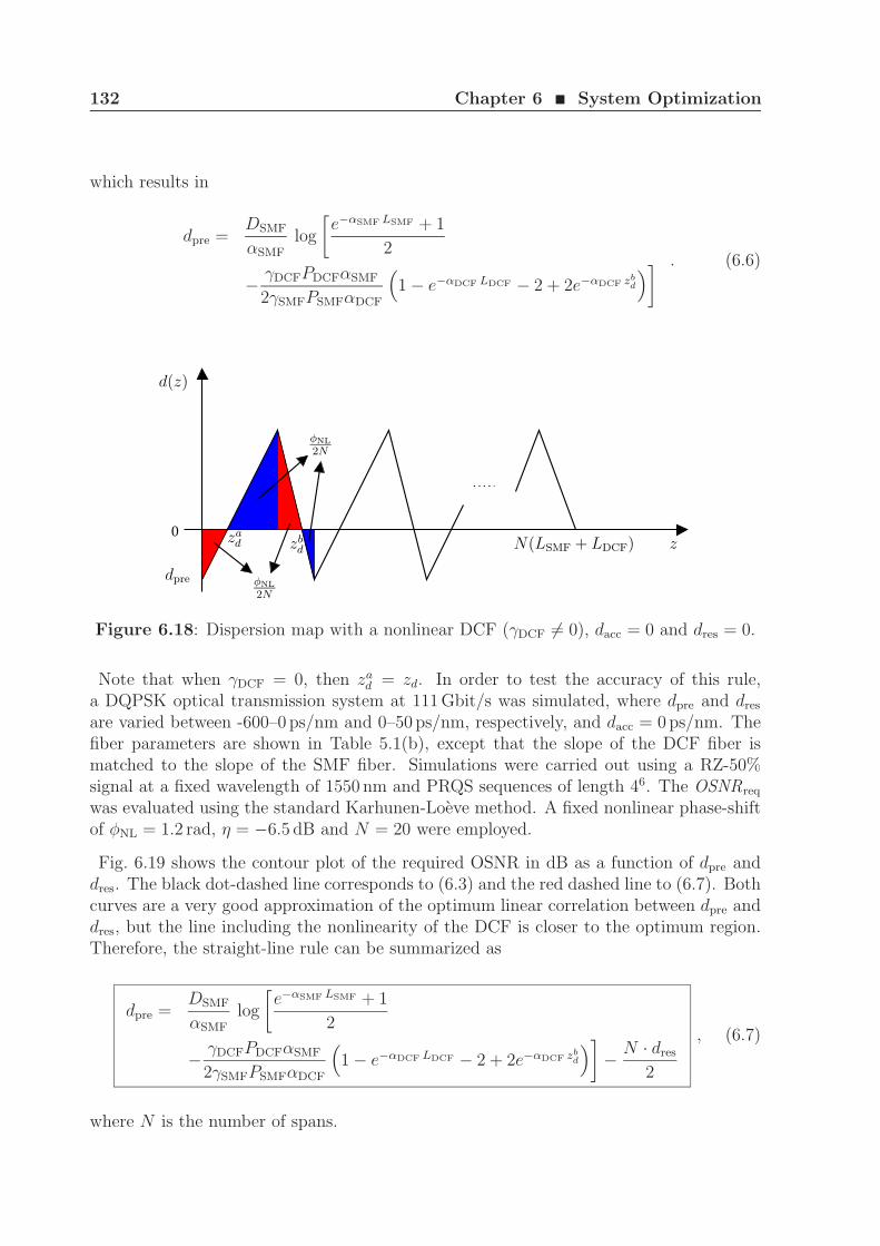
132 Chapter 6 ¥ System Optimization
which results in
dpre =DSMF
αSMF
log
[e−αSMF LSMF + 1
2
− γDCFPDCFαSMF
2γSMFPSMFαDCF
(1 − e−αDCF LDCF − 2 + 2e−αDCF zb
d
)] . (6.6)
0 zad
d(z)
dpre
zN(LSMF + LDCF)
φNL
2N
zbd
φNL
2N
Figure 6.18: Dispersion map with a nonlinear DCF (γDCF 6= 0), dacc = 0 and dres = 0.
Note that when γDCF = 0, then zad = zd. In order to test the accuracy of this rule,
a DQPSK optical transmission system at 111 Gbit/s was simulated, where dpre and dres
are varied between -600–0 ps/nm and 0–50 ps/nm, respectively, and dacc = 0 ps/nm. Thefiber parameters are shown in Table 5.1(b), except that the slope of the DCF fiber ismatched to the slope of the SMF fiber. Simulations were carried out using a RZ-50%signal at a fixed wavelength of 1550 nm and PRQS sequences of length 46. The OSNRreq
was evaluated using the standard Karhunen-Loeve method. A fixed nonlinear phase-shiftof φNL = 1.2 rad, η = −6.5 dB and N = 20 were employed.
Fig. 6.19 shows the contour plot of the required OSNR in dB as a function of dpre anddres. The black dot-dashed line corresponds to (6.3) and the red dashed line to (6.7). Bothcurves are a very good approximation of the optimum linear correlation between dpre anddres, but the line including the nonlinearity of the DCF is closer to the optimum region.Therefore, the straight-line rule can be summarized as
dpre =DSMF
αSMF
log
[e−αSMF LSMF + 1
2
− γDCFPDCFαSMF
2γSMFPSMFαDCF
(1 − e−αDCF LDCF − 2 + 2e−αDCF zb
d
)]− N · dres
2
, (6.7)
where N is the number of spans.
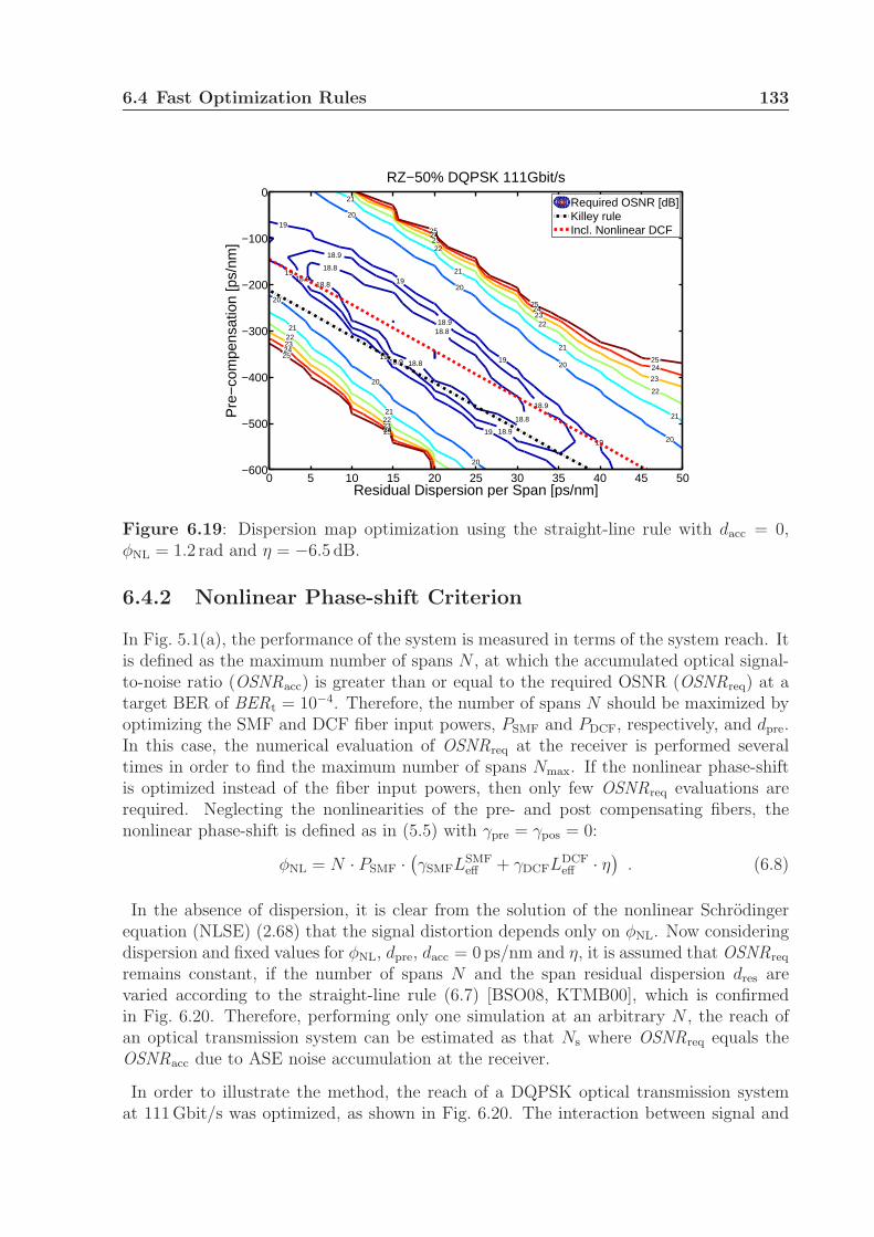
6.4 Fast Optimization Rules 133
18.8
18.8
18.8
18.8
18.8
18.9
18.9
18.9
18.9
18.9
18.9
19
19
19
19
19
19
1920
20
20
20
20
20
20
21
21
21
2121
21
22
22
22
22
22
23
23
23
23
23
24
24
24
24
24
25
25
25
25
25
Residual Dispersion per Span [ps/nm]
Pre
−co
mpe
nsat
ion
[ps/
nm]
RZ−50% DQPSK 111Gbit/s
0 5 10 15 20 25 30 35 40 45 50−600
−500
−400
−300
−200
−100
0Required OSNR [dB]Killey ruleIncl. Nonlinear DCF
Figure 6.19: Dispersion map optimization using the straight-line rule with dacc = 0,φNL = 1.2 rad and η = −6.5 dB.
6.4.2 Nonlinear Phase-shift Criterion
In Fig. 5.1(a), the performance of the system is measured in terms of the system reach. Itis defined as the maximum number of spans N , at which the accumulated optical signal-to-noise ratio (OSNRacc) is greater than or equal to the required OSNR (OSNRreq) at atarget BER of BERt = 10−4. Therefore, the number of spans N should be maximized byoptimizing the SMF and DCF fiber input powers, PSMF and PDCF, respectively, and dpre.In this case, the numerical evaluation of OSNRreq at the receiver is performed severaltimes in order to find the maximum number of spans Nmax. If the nonlinear phase-shiftis optimized instead of the fiber input powers, then only few OSNRreq evaluations arerequired. Neglecting the nonlinearities of the pre- and post compensating fibers, thenonlinear phase-shift is defined as in (5.5) with γpre = γpos = 0:
φNL = N · PSMF ·(γSMFLSMF
eff + γDCFLDCFeff · η
). (6.8)
In the absence of dispersion, it is clear from the solution of the nonlinear Schrodingerequation (NLSE) (2.68) that the signal distortion depends only on φNL. Now consideringdispersion and fixed values for φNL, dpre, dacc = 0 ps/nm and η, it is assumed that OSNRreq
remains constant, if the number of spans N and the span residual dispersion dres arevaried according to the straight-line rule (6.7) [BSO08, KTMB00], which is confirmedin Fig. 6.20. Therefore, performing only one simulation at an arbitrary N , the reach ofan optical transmission system can be estimated as that Ns where OSNRreq equals theOSNRacc due to ASE noise accumulation at the receiver.
In order to illustrate the method, the reach of a DQPSK optical transmission systemat 111 Gbit/s was optimized, as shown in Fig. 6.20. The interaction between signal and
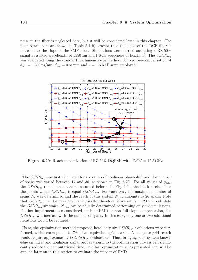
134 Chapter 6 ¥ System Optimization
noise in the fiber is neglected here, but it will be considered later in this chapter. Thefiber parameters are shown in Table 5.1(b), except that the slope of the DCF fiber ismatched to the slope of the SMF fiber. Simulations were carried out using a RZ-50%signal at a fixed wavelength of 1550 nm and PRQS sequences of length 46. The OSNRreq
was evaluated using the standard Karhunen-Loeve method. A fixed pre-compensation ofdpre = −300 ps/nm, dacc = 0 ps/nm and η = −6.5 dB were employed.
17 18 19 20 21 22 23 24 25 26 27 28 29 3017
18
19
20
21
22
23
24
Number of Spans
OS
NR
[dB
]
RZ−50% DQPSK 111 Gbit/s
φNL
=0.4 rad OSNRacc
φNL
=0.4 rad OSNRreq
φNL
=0.6 rad OSNRacc
φNL
=0.6 rad OSNRreq
φNL
=0.8 rad OSNRacc
φNL
=0.8 rad OSNRreq
φNL
=1.0 rad OSNRacc
φNL
=1.0 rad OSNRreq
φNL
=1.2 rad OSNRacc
φNL
=1.2 rad OSNRreq
φNL
=1.4 rad OSNRacc
φNL
=1.4 rad OSNRreq
Optimum: φNL
= 1.2 radN
max= 26 spans
Figure 6.20: Reach maximization of RZ-50% DQPSK with RBW = 12.5 GHz.
The OSNRreq was first calculated for six values of nonlinear phase-shift and the numberof spans was varied between 17 and 30, as shown in Fig. 6.20. For all values of φNL,the OSNRreq remains constant as assumed before. In Fig. 6.20, the black circles showthe points where OSNRreq is equal OSNRacc. For each φNL, the maximum number ofspans Ns was determined and the reach of this system Nmax amounts to 26 spans. Notethat OSNRacc can be calculated analytically, therefore, if we set N = 20 and calculatethe OSNRreq six times, Nmax can be equally determined performing only six simulations.If other impairments are considered, such as PMD or non full slope compensation, theOSNRreq will increase with the number of spans. In this case, only one or two additionaliterations would be required.
Using the optimization method proposed here, only six OSNRreq evaluations were per-formed, which corresponds to 7% of an equivalent grid search. A complete grid searchwould require approximately 78 OSNRreq evaluations. Thus, bringing some system knowl-edge on linear and nonlinear signal propagation into the optimization process can signifi-cantly reduce the computational time. The fast optimization rules presented here will beapplied later on in this section to evaluate the impact of PMD.
6.5 Global Optimization 135
6.5 Global Optimization
In fiber-optic communication systems, the main source of performance degradation are theaccumulated amplified spontaneous emission (ASE) noise, polarization-mode dispersion(PMD) and fiber dispersion and nonlinearity. The bit-error rate for systems containingall these impairments and their interactions with the signal can be calculated using thestandard Monte Carlo method. However, if the BER has to be computed very often, theoverall computational effort is so large that it becomes prohibitive for system optimization.In this case, the BER can be calculated very fast and accurate by using linearizationtechniques of the Nonlinear Schrodinger Equation (NLSE) together with Karhunen-Loeveseries expansion, as explained in detail in Chapter 4.
Even using these semi-analytical methods for calculating the BER, the optimizationprocedure can still be very time-consuming if, for example, grid search algorithms areemployed, i.e. every variable is varied independently within a pre-defined range. Severalfast optimization methods have been investigated, but all of them use simplified modelsfor nonlinear signal propagation and, therefore, are only valid for a certain range ofparameters or modulation formats [EFS+00, ABF02, KTMB00, BSO08]. In this context,global optimization algorithms can be employed to guide the search over the large setof parameters in order to find the best solution in the minimum simulation time. Theyare independent of external parameters and converge to the global optimum, reducingthe number of required simulations. After the optimization procedure, simplified modelsmay be used to include PMD, which would require a large computational effort at eachiteration of the optimization algorithm.
In this section, a global optimization algorithm is derived and applied together with thestandard Karhunen-Loeve method in order to find the maximum reach of single-channelOOK, DPSK and DQPSK systems at several data rates. Following, using the extendedKarhunen-Loeve method, the nonlinear phase-shift criterion and the straight-line rule,the impact of PMD and nonlinear phase noise on the global optimization of DPSK andDQPSK systems is investigated for data rates ranging from 5 Gbit/s to 230 Gbit/s.
6.5.1 The Global Optimization Algorithm
In many engineering problems, we are often interested in finding the maximum1 of an ob-jective function. If the objective function is strictly convex, i.e. it has only one maximum,then the optimization problem can be solved using several local algorithms [PTVF07]. Ifthe objective function is not convex, i.e. it has many local maxima and one or moreglobal maxima, then global optimization algorithms should be applied. In this work, weare going to focus on global optimization problems, where the objective function is com-putationally expensive to evaluate. It means that the global maximum should be foundin as few iterations as possible. For instance, this is the case of the calculation of theBER or required OSNR after the optical signal propagation through a link.
1In this work, the algorithm is implemented to maximize the objective function. In fact, there is nodifference between minimizing and maximizing since the maximum of f is the minimum of −f .
136 Chapter 6 ¥ System Optimization
Formally, we are concerned with the problem of finding x∗ ∈ D such that f(x∗) ≥ f(x)for all x ∈ D, where D is the search space. If d input parameters should be optimized,then the problem dimension is defined as d and D is a compact subset of Rd. Theobjective function f : D → R is defined as a general unknown continuous function,x = [x1 x2 · · · xd]
T is the input vector and [·]T is the matrix transpose operator. Eachvariable xi is upper and lower bounded, which forms a hypercube in Rd.
Initially, the algorithm simulates the 2d boundary points, then it divides the searchspace into disjoint sub-regions. These sub-regions are obtained by using the Delaunaytriangulation [Eld92] where each of their d + 1 vertices corresponds to a simulated point.Geometrically, each sub-region is a simplex (triangle for d = 2 or tetrahedron for d = 3).As a result the unknown objective function is approximated over a bounded space by aset of simplexes.
At any given point x ∈ Sk, where Sk ⊂ D is the region delimited by the simplex k, theobjective function f(x) is modeled as a sample function of a Gaussian random process,i.e. a Brownian motion process [Kus64, Jon01, Gut01]. Its mean µk
f (x) = Ef(x) and
variance (σkf )2(x) = E(f(x) − µk
f )2 are used to find the next set of input parameters
x, which will most probably improve the currently best solution x∗. Mathematically, itcan be written as
Pk(f(x) > f(x∗) + εi) = 1 − Φ(√
D2(x))
, (6.9)
where
D2(x) =
(f(x∗) + εi − µk
f (x))2
(σkf )2(x)
(6.10)
µkf (x) = aT ·
[x
1
](6.11)
(σkf )2(x) =
[xT 1
]· C ·
[x
1
], (6.12)
Φ(·) is the normal cumulative distribution function, εi is a positive real number at theiteration i, a is a (d + 1)× 1 vector and C is a symmetrical (d + 1)× (d + 1) matrix. Thevector a and matrix C are unknown and can be calculated as follows: x is deterministicwhile f(x) is modeled as a Gaussian stochastic process. Therefore, for each x ∈ Dthere is a corresponding mean and variance. At the vertices of the simplex k, the meanµk
f (xv) and variance (σkf )2(xv) are known and given by f(xv) and 0, respectively, where
v ∈ 1, 2, . . . , d+1. Consequently, the vector a can be calculated using the d+1 verticesof the simplex. Due to the symmetry of the matrix C, the vertices and midpoints xm areenough to calculate all elements of C. The midpoints are defined such that (σk
f )2(xm) =ηi · ‖xp −xq‖, where ‖xp −xq‖ is the Euclidean distance between the vertices xp and xq
and ηi is the mean squared variation in f(x) as x changes at the iteration i.
In (6.9), we want to find the point xk ∈ Sk that gives the highest probability of improve-ment Pk for the simplex k, i.e.
xk = arg max[1 − Φ
(√D2(x)
)]= arg min
[D2(x)
]. (6.13)

6.5 Global Optimization 137
For each simplex there is only one point xk, where Pk is maximum because the functionin (6.13) is convex. Therefore, the point xk with the highest probability Pk among allsimplexes is the choice of parameters for the next simulation.
As stated before, the algorithm is based on the assumption that the objective function isnormally distributed at each point. However, for most practical applications, the objectivefunction f(x) assumes values within a certain finite interval. For example, the requiredOSNR in dB is normally a positive number between 5 and 60 dB. This kind of informationcan be used to improve the convergence of the algorithm [Per89]. One technique widelyused in non-parametric statistics is the rank transformation. Ranking the objective func-tion evaluations allows the algorithm to be unaffected by the location and scale of thefunction. Moreover, all calculations described before can be performed on the rankedobjective function evaluations rather than on the actual evaluations themselves and thestatistical method’s validity no longer depends on the normality of the data. By setting apredetermined number of iterations Ni, the number of function evaluations at the end ofthe optimization procedure will be 2d+Ni. Therefore, after the iteration i−1, a vector with
the function evaluations can be defined as F =[f(x1) f(x2) . . . f(x2d
) . . . f(x2d+i−1)]T
,
where f(x2d+i−1) is the function evaluation at the iteration i − 1. Ranking the vector F
results in another vector F r of the same size, where each element is a natural numberbetween 1 and 2d + i − 1. The next set of input parameters xi is obtained by using F r
and the set of simplexes.
One of the main problems in global optimization is the balance between local and globalsearch at each iteration. Actually, any global optimization algorithm must have a featurethat forces it to pay attention to parts of the search space that have been relativelyunexplored. In (6.9), the ratio between the mean µk
f (x), which is maximum for values
close to f(x∗), and the variance (σkf )2(x), which is maximum in unexplored regions of the
search space, implements this feature and, therefore, guarantees the global convergence ofthe algorithm [Jon01]. The role of the constant εi is to set the balance between local andglobal search. High values of εi will make the search global, while low values local. Bysetting εi = Ni − i + 1, the algorithm first explores the search space, then it focusses onregions of interest and finally refines the search until εNi = 1. However, it is possible thatthe search stays too long in global mode or too long in local mode. Therefore, an additionalloop feedback can be used in order to choose εi adaptively for each iteration [Per89], asshown in Fig. 6.21. Based on M previous iterations, εi can be set according to thefollowing equations:
RR(i) =F r(2
d + i − 1) − 1
2d + i − 2(6.14)
MA(i) =
1i
∑i
j=1 RR(i − j + 1), M ≤ i;1M
∑M
j=1 RR(i − j + 1), M > i.(6.15)
εi = (Ni − i) · MA(i) + 1 , (6.16)
where RR is defined as the rank ratio and MA is a moving average to statistically forecastthe next rank ratio. RR(1) is defined as 1, RR(i) is equal 1, if F r(2
d + i− 1) = 2d + i− 1
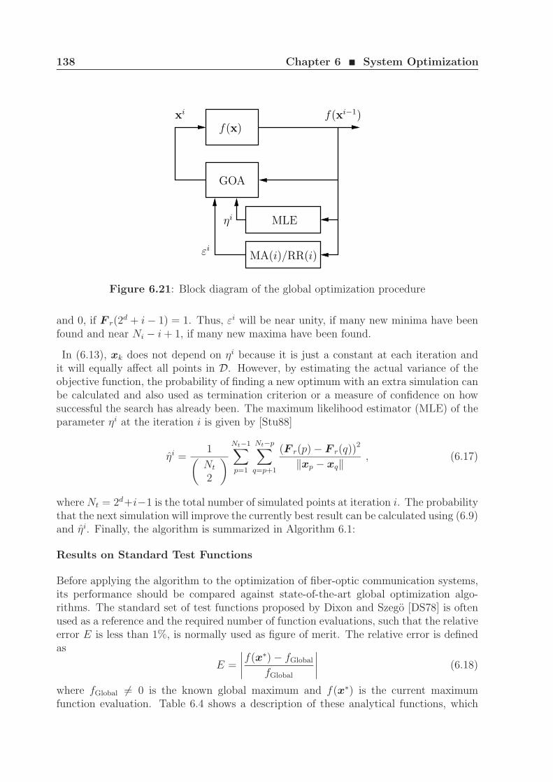
138 Chapter 6 ¥ System Optimization
f(xi−1)f(x)
GOA
xi
MLE
MA(i)/RR(i)
ηi
εi
Figure 6.21: Block diagram of the global optimization procedure
and 0, if F r(2d + i − 1) = 1. Thus, εi will be near unity, if many new minima have been
found and near Ni − i + 1, if many new maxima have been found.
In (6.13), xk does not depend on ηi because it is just a constant at each iteration andit will equally affect all points in D. However, by estimating the actual variance of theobjective function, the probability of finding a new optimum with an extra simulation canbe calculated and also used as termination criterion or a measure of confidence on howsuccessful the search has already been. The maximum likelihood estimator (MLE) of theparameter ηi at the iteration i is given by [Stu88]
ηi =1(Nt
2
)Nt−1∑
p=1
Nt−p∑
q=p+1
(F r(p) − F r(q))2
‖xp − xq‖, (6.17)
where Nt = 2d+i−1 is the total number of simulated points at iteration i. The probabilitythat the next simulation will improve the currently best result can be calculated using (6.9)and ηi. Finally, the algorithm is summarized in Algorithm 6.1:
Results on Standard Test Functions
Before applying the algorithm to the optimization of fiber-optic communication systems,its performance should be compared against state-of-the-art global optimization algo-rithms. The standard set of test functions proposed by Dixon and Szego [DS78] is oftenused as a reference and the required number of function evaluations, such that the relativeerror E is less than 1%, is normally used as figure of merit. The relative error is definedas
E =
∣∣∣∣f(x∗) − fGlobal
fGlobal
∣∣∣∣ (6.18)
where fGlobal 6= 0 is the known global maximum and f(x∗) is the current maximumfunction evaluation. Table 6.4 shows a description of these analytical functions, which
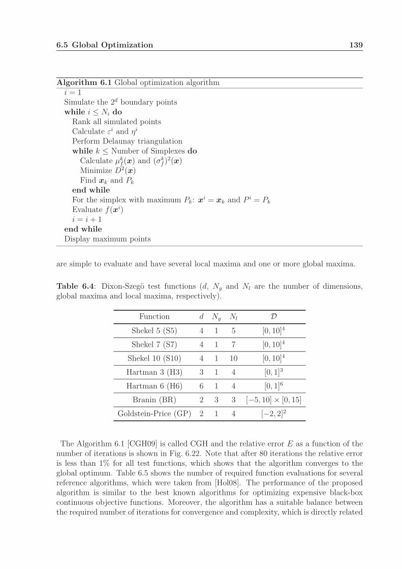
6.5 Global Optimization 139
Algorithm 6.1 Global optimization algorithmi = 1Simulate the 2d boundary pointswhile i ≤ Ni do
Rank all simulated pointsCalculate εi and ηi
Perform Delaunay triangulationwhile k ≤ Number of Simplexes do
Calculate µkf (x) and (σk
f )2(x)Minimize D2(x)Find xk and Pk
end whileFor the simplex with maximum Pk: xi = xk and P i = Pk
Evaluate f(xi)i = i + 1
end whileDisplay maximum points
are simple to evaluate and have several local maxima and one or more global maxima.
Table 6.4: Dixon-Szego test functions (d, Ng and Nl are the number of dimensions,global maxima and local maxima, respectively).
Function d Ng Nl DShekel 5 (S5) 4 1 5 [0, 10]4
Shekel 7 (S7) 4 1 7 [0, 10]4
Shekel 10 (S10) 4 1 10 [0, 10]4
Hartman 3 (H3) 3 1 4 [0, 1]3
Hartman 6 (H6) 6 1 4 [0, 1]6
Branin (BR) 2 3 3 [−5, 10] × [0, 15]
Goldstein-Price (GP) 2 1 4 [−2, 2]2
The Algorithm 6.1 [CGH09] is called CGH and the relative error E as a function of thenumber of iterations is shown in Fig. 6.22. Note that after 80 iterations the relative erroris less than 1% for all test functions, which shows that the algorithm converges to theglobal optimum. Table 6.5 shows the number of required function evaluations for severalreference algorithms, which were taken from [Hol08]. The performance of the proposedalgorithm is similar to the best known algorithms for optimizing expensive black-boxcontinuous objective functions. Moreover, the algorithm has a suitable balance betweenthe required number of iterations for convergence and complexity, which is directly related
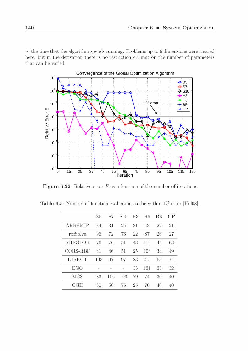
140 Chapter 6 ¥ System Optimization
to the time that the algorithm spends running. Problems up to 6 dimensions were treatedhere, but in the derivation there is no restriction or limit on the number of parametersthat can be varied.
5 15 25 35 45 55 65 75 85 95 105 115 12510
−6
10−5
10−4
10−3
10−2
10−1
100
101
Iteration
Rel
ativ
e E
rror
E
Convergence of the Global Optimization Algorithm
S5S7S10H3H6BRGP
1 % error
Figure 6.22: Relative error E as a function of the number of iterations
Table 6.5: Number of function evaluations to be within 1% error [Hol08].
S5 S7 S10 H3 H6 BR GP
ARBFMIP 34 31 25 31 43 22 21
rbfSolve 96 72 76 22 87 26 27
RBFGLOB 76 76 51 43 112 44 63
CORS-RBF 41 46 51 25 108 34 49
DIRECT 103 97 97 83 213 63 101
EGO - - - 35 121 28 32
MCS 83 106 103 79 74 30 40
CGH 80 50 75 25 70 40 40
6.5 Global Optimization 141
6.5.2 Optimization and System Set-up
Now the global optimization algorithm will be used to optimize the performance of fiber-optic communication systems. Fig. 5.1 shows a typical system comprising N spans. Thenonlinearity of the pre- and post-compensation fibers is neglected, but their attenuationsare taken into account. The fiber parameters are shown in Table 5.1(b). Simulations werecarried out using non-return-to-zero (NRZ) pulse format and PRBS/PRQS sequences oflength 45. The fibers were numerically simulated by solving the scalar NLSE (2.66).The optical filter was modeled as a second-order Gaussian filter and its bandwidth wasoptimized for each data rate in a back-to-back configuration. The electrical filter wasmodeled as a fifth-order Bessel filter with a bandwidth of 0.75 ·Rs, where Rs is the symbolrate.
The performance of the system is measured in terms of the system reach. It is defined asthe maximum number of spans N , at which the accumulated OSNRacc is equal or greaterthan the required OSNRreq at a target BER of 10−4. The optimization problem can beformally written as N = f(PSMF, PDCF, dpre, dres, dacc), where f(·) is the objective functionand S = PSMF, PDCF, dpre, dres, dacc the five-dimensional search space. For each data rateRb, the algorithm tries to find iteratively the set of input parameters, which maximizesthe system reach, i.e.
Nmax = f(P optSMF, P opt
DCF, doptpre, d
optres , d
optacc) . (6.19)
The global optimization algorithm starts by simulating the 25 boundary points, thenit divides the search space into a set of simplexes. For each simplex, the variable N ismodeled as a Gaussian stochastic process and its mean µN and variance σ2
N are used inorder to find the next set of input parameters, which will most probably improve thecurrently best solution N∗
max. Mathematically, it can be written as
P (N > N∗max + ε) = 1 − Φ
(N∗
max + ε − µN√σ2
N
), (6.20)
where Φ(·) is the cumulative normal density function and ε a positive real number usedto set the balance between local and global search. Considering all sub-regions, the pointwith the highest probability of improvement is simulated and, including the new point, thesearch space is again divided into sub-regions. Any global optimization algorithm musthave a feature that forces it to pay attention to parts of the search space that have beenrelatively unexplored. In (6.20), the balance between the mean µN , which is maximum forvalues close to N∗
max, and the variance σ2N , which is maximum in unexplored regions of the
search space, implements this feature and, therefore, guarantees the global convergenceof the algorithm [Jon01].
In Fig. 6.22, considering all test functions, the minimum number of iterations re-quired by the algorithm to converge is 80. Therefore, the number of iterations was setto Ni = 200, which corresponds to approximately 0.01% simulations of an equivalentgrid search. After Ni iterations the global optimization algorithm determines Nmax and
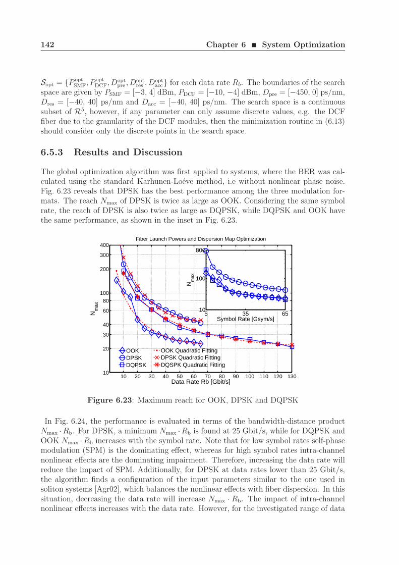
142 Chapter 6 ¥ System Optimization
Sopt = P optSMF, P opt
DCF, Doptpre , D
optres , Dopt
acc for each data rate Rb. The boundaries of the searchspace are given by PSMF = [−3, 4] dBm, PDCF = [−10, −4] dBm, Dpre = [−450, 0] ps/nm,Dres = [−40, 40] ps/nm and Dacc = [−40, 40] ps/nm. The search space is a continuoussubset of R5, however, if any parameter can only assume discrete values, e.g. the DCFfiber due to the granularity of the DCF modules, then the minimization routine in (6.13)should consider only the discrete points in the search space.
6.5.3 Results and Discussion
The global optimization algorithm was first applied to systems, where the BER was cal-culated using the standard Karhunen-Loeve method, i.e without nonlinear phase noise.Fig. 6.23 reveals that DPSK has the best performance among the three modulation for-mats. The reach Nmax of DPSK is twice as large as OOK. Considering the same symbolrate, the reach of DPSK is also twice as large as DQPSK, while DQPSK and OOK havethe same performance, as shown in the inset in Fig. 6.23.
10 20 30 40 50 60 70 80 90 100 110 120 13010
20
30
40
60
80
100
200
300
400
Data Rate Rb [Gbit/s]
Nm
ax
Fiber Launch Powers and Dispersion Map Optimization
5 35 6510
100
800
Symbol Rate [Gsym/s]
Nm
ax
OOK OOK Quadratic FittingDPSK DPSK Quadratic FittingDQPSK DQSPK Quadratic Fitting
Figure 6.23: Maximum reach for OOK, DPSK and DQPSK
In Fig. 6.24, the performance is evaluated in terms of the bandwidth-distance productNmax ·Rb. For DPSK, a minimum Nmax ·Rb is found at 25 Gbit/s, while for DQPSK andOOK Nmax ·Rb increases with the symbol rate. Note that for low symbol rates self-phasemodulation (SPM) is the dominating effect, whereas for high symbol rates intra-channelnonlinear effects are the dominating impairment. Therefore, increasing the data rate willreduce the impact of SPM. Additionally, for DPSK at data rates lower than 25 Gbit/s,the algorithm finds a configuration of the input parameters similar to the one used insoliton systems [Agr02], which balances the nonlinear effects with fiber dispersion. In thissituation, decreasing the data rate will increase Nmax · Rb. The impact of intra-channelnonlinear effects increases with the data rate. However, for the investigated range of data
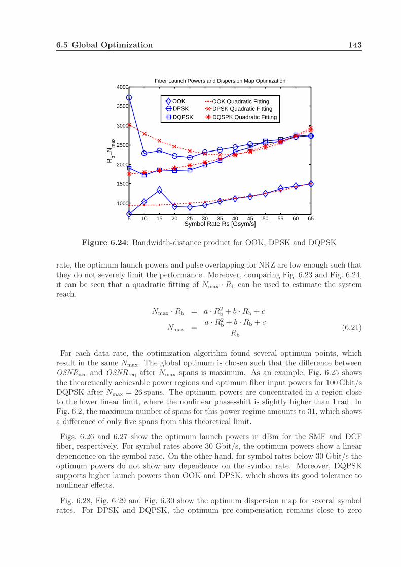
6.5 Global Optimization 143
5 10 15 20 25 30 35 40 45 50 55 60 65
1000
1500
2000
2500
3000
3500
4000
Symbol Rate Rs [Gsym/s]
Rb⋅ N
max
Fiber Launch Powers and Dispersion Map Optimization
OOK OOK Quadratic FittingDPSK DPSK Quadratic FittingDQPSK DQSPK Quadratic Fitting
Figure 6.24: Bandwidth-distance product for OOK, DPSK and DQPSK
rate, the optimum launch powers and pulse overlapping for NRZ are low enough such thatthey do not severely limit the performance. Moreover, comparing Fig. 6.23 and Fig. 6.24,it can be seen that a quadratic fitting of Nmax · Rb can be used to estimate the systemreach.
Nmax · Rb = a · R2b + b · Rb + c
Nmax =a · R2
b + b · Rb + c
Rb
(6.21)
For each data rate, the optimization algorithm found several optimum points, whichresult in the same Nmax. The global optimum is chosen such that the difference betweenOSNRacc and OSNRreq after Nmax spans is maximum. As an example, Fig. 6.25 showsthe theoretically achievable power regions and optimum fiber input powers for 100 Gbit/sDQPSK after Nmax = 26 spans. The optimum powers are concentrated in a region closeto the lower linear limit, where the nonlinear phase-shift is slightly higher than 1 rad. InFig. 6.2, the maximum number of spans for this power regime amounts to 31, which showsa difference of only five spans from this theoretical limit.
Figs. 6.26 and 6.27 show the optimum launch powers in dBm for the SMF and DCFfiber, respectively. For symbol rates above 30 Gbit/s, the optimum powers show a lineardependence on the symbol rate. On the other hand, for symbol rates below 30 Gbit/s theoptimum powers do not show any dependence on the symbol rate. Moreover, DQPSKsupports higher launch powers than OOK and DPSK, which shows its good tolerance tononlinear effects.
Fig. 6.28, Fig. 6.29 and Fig. 6.30 show the optimum dispersion map for several symbolrates. For DPSK and DQPSK, the optimum pre-compensation remains close to zero
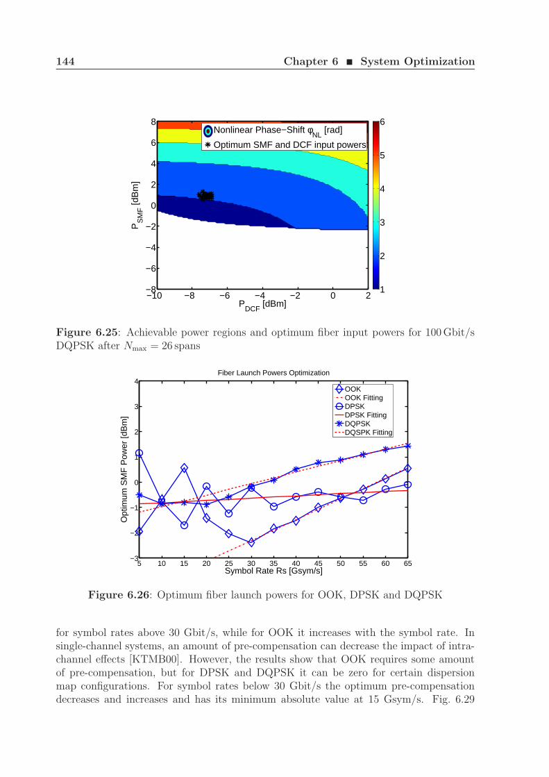
144 Chapter 6 ¥ System Optimization
PDCF
[dBm]
PS
MF [d
Bm
]
−10 −8 −6 −4 −2 0 2−8
−6
−4
−2
0
2
4
6
8
1
2
3
4
5
6Nonlinear Phase−Shift φ
NL [rad]
Optimum SMF and DCF input powers
Figure 6.25: Achievable power regions and optimum fiber input powers for 100 Gbit/sDQPSK after Nmax = 26 spans
5 10 15 20 25 30 35 40 45 50 55 60 65−3
−2
−1
0
1
2
3
4
Symbol Rate Rs [Gsym/s]
Opt
imum
SM
F P
ower
[dB
m]
Fiber Launch Powers Optimization
OOKOOK FittingDPSKDPSK FittingDQPSKDQSPK Fitting
Figure 6.26: Optimum fiber launch powers for OOK, DPSK and DQPSK
for symbol rates above 30 Gbit/s, while for OOK it increases with the symbol rate. Insingle-channel systems, an amount of pre-compensation can decrease the impact of intra-channel effects [KTMB00]. However, the results show that OOK requires some amountof pre-compensation, but for DPSK and DQPSK it can be zero for certain dispersionmap configurations. For symbol rates below 30 Gbit/s the optimum pre-compensationdecreases and increases and has its minimum absolute value at 15 Gsym/s. Fig. 6.29
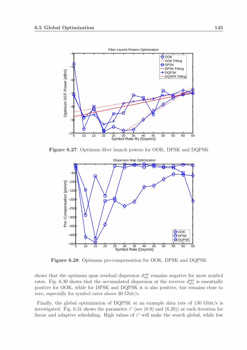
6.5 Global Optimization 145
5 10 15 20 25 30 35 40 45 50 55 60 65−10
−9
−8
−7
−6
−5
−4
Symbol Rate Rs [Gsym/s]
Opt
imum
DC
F P
ower
[dB
m]
Fiber Launch Powers Optimization
OOKOOK FittingDPSKDPSK FittingDQPSKDQSPK Fitting
Figure 6.27: Optimum fiber launch powers for OOK, DPSK and DQPSK
5 10 15 20 25 30 35 40 45 50 55 60 65−450
−400
−350
−300
−250
−200
−150
−100
−50
0
Symbol Rate [Gsym/s]
Pre
−C
ompe
nsat
ion
[ps/
nm]
Dispersion Map Optimization
OOKDPSKDQPSK
Figure 6.28: Optimum pre-compensation for OOK, DPSK and DQPSK
shows that the optimum span residual dispersion doptres remains negative for most symbol
rates. Fig. 6.30 shows that the accumulated dispersion at the receiver doptacc is essentially
positive for OOK, while for DPSK and DQPSK it is also positive, but remains close tozero, especially for symbol rates above 30 Gbit/s.
Finally, the global optimization of DQPSK at an example data rate of 130 Gbit/s isinvestigated. Fig. 6.31 shows the parameter εi (see (6.9) and (6.20)) at each iteration forlinear and adaptive scheduling. High values of εi will make the search global, while low

146 Chapter 6 ¥ System Optimization
5 10 15 20 25 30 35 40 45 50 55 60 65−20
−15
−10
−5
0
5
10
15
20
Symbol Rate [Gsym/s]
Res
idua
l Dis
pers
ion
[ps/
nm]
Dispersion Map Optimization
OOKDPSKDQPSK
Figure 6.29: Optimum span residual dispersion for OOK, DPSK and DQPSK
5 10 15 20 25 30 35 40 45 50 55 60 65−20
−10
0
10
20
30
40
Symbol Rate [Gsym/s]
Acc
umul
ated
Dis
pers
ion
[ps/
nm]
Dispersion Map Optimization
OOKDPSKDQPSK
Figure 6.30: Optimum accumulated dispersion for OOK, DPSK and DQPSK
values local. Thus, each local minimum in the figure indicates that a value close to thecurrent maximum was found. Fig. 6.32 shows the relation between dopt
pre and doptres . It can be
observed that the optimum points lie on a line almost parallel to (6.3) and (6.7), like thosedepicted in Fig. 6.19. A good approximation is achieved, when the nonlinearity of theDCF is considered. This result shows that simplified models can be a fair approximation.However, they might fail for certain system configurations. Therefore, global optimizationis the most appropriate procedure for efficient and accurate system optimization.
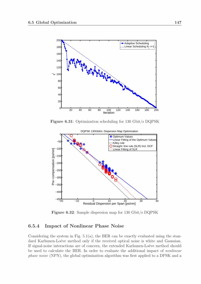
6.5 Global Optimization 147
20 40 60 80 100 120 140 160 180 2000
20
40
60
80
100
120
140
160
180
200
Iteration
εi
Adaptive SchedulingLinear Scheduling N
i−i+1
Figure 6.31: Optimization scheduling for 130 Gbit/s DQPSK
−20 −10 0 10 20 30 40−450
−400
−350
−300
−250
−200
−150
−100
−50
0
Residual Dispersion per Span [ps/nm]
Pre
−co
mpe
nsat
ion
[ps/
nm]
DQPSK 130Gbit/s: Dispersion Map Optimization
Optimum ValuesLinear Fitting of the Optimum ValuesKilley ruleStraight−line rule (SLR) Incl. DCFLinear Fitting of SLR
Figure 6.32: Sample dispersion map for 130 Gbit/s DQPSK
6.5.4 Impact of Nonlinear Phase Noise
Considering the system in Fig. 5.1(a), the BER can be exactly evaluated using the stan-dard Karhunen-Loeve method only if the received optical noise is white and Gaussian.If signal-noise interactions are of concern, the extended Karhunen-Loeve method shouldbe used to calculate the BER. In order to evaluate the additional impact of nonlinearphase noise (NPN), the global optimization algorithm was first applied to a DPSK and a
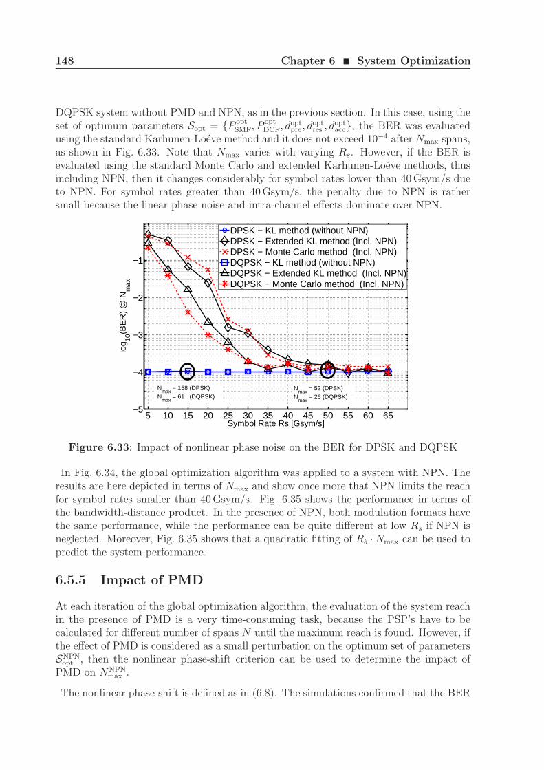
148 Chapter 6 ¥ System Optimization
DQPSK system without PMD and NPN, as in the previous section. In this case, using theset of optimum parameters Sopt = P opt
SMF, P optDCF, dopt
pre, doptres , d
optacc, the BER was evaluated
using the standard Karhunen-Loeve method and it does not exceed 10−4 after Nmax spans,as shown in Fig. 6.33. Note that Nmax varies with varying Rs. However, if the BER isevaluated using the standard Monte Carlo and extended Karhunen-Loeve methods, thusincluding NPN, then it changes considerably for symbol rates lower than 40 Gsym/s dueto NPN. For symbol rates greater than 40 Gsym/s, the penalty due to NPN is rathersmall because the linear phase noise and intra-channel effects dominate over NPN.
5 10 15 20 25 30 35 40 45 50 55 60 65−5
−4
−3
−2
−1
Symbol Rate Rs [Gsym/s]
log 10
(BE
R)
@ N
max
DPSK − KL method (without NPN)DPSK − Extended KL method (Incl. NPN)DPSK − Monte Carlo method (Incl. NPN)DQPSK − KL method (without NPN)DQPSK − Extended KL method (Incl. NPN)DQPSK − Monte Carlo method (Incl. NPN)
Nmax
= 158 (DPSK)N
max = 61 (DQPSK)
Nmax
= 52 (DPSK)N
max = 26 (DQPSK)
Figure 6.33: Impact of nonlinear phase noise on the BER for DPSK and DQPSK
In Fig. 6.34, the global optimization algorithm was applied to a system with NPN. Theresults are here depicted in terms of Nmax and show once more that NPN limits the reachfor symbol rates smaller than 40 Gsym/s. Fig. 6.35 shows the performance in terms ofthe bandwidth-distance product. In the presence of NPN, both modulation formats havethe same performance, while the performance can be quite different at low Rs if NPN isneglected. Moreover, Fig. 6.35 shows that a quadratic fitting of Rb · Nmax can be used topredict the system performance.
6.5.5 Impact of PMD
At each iteration of the global optimization algorithm, the evaluation of the system reachin the presence of PMD is a very time-consuming task, because the PSP’s have to becalculated for different number of spans N until the maximum reach is found. However, ifthe effect of PMD is considered as a small perturbation on the optimum set of parametersSNPN
opt , then the nonlinear phase-shift criterion can be used to determine the impact ofPMD on NNPN
max .
The nonlinear phase-shift is defined as in (6.8). The simulations confirmed that the BER
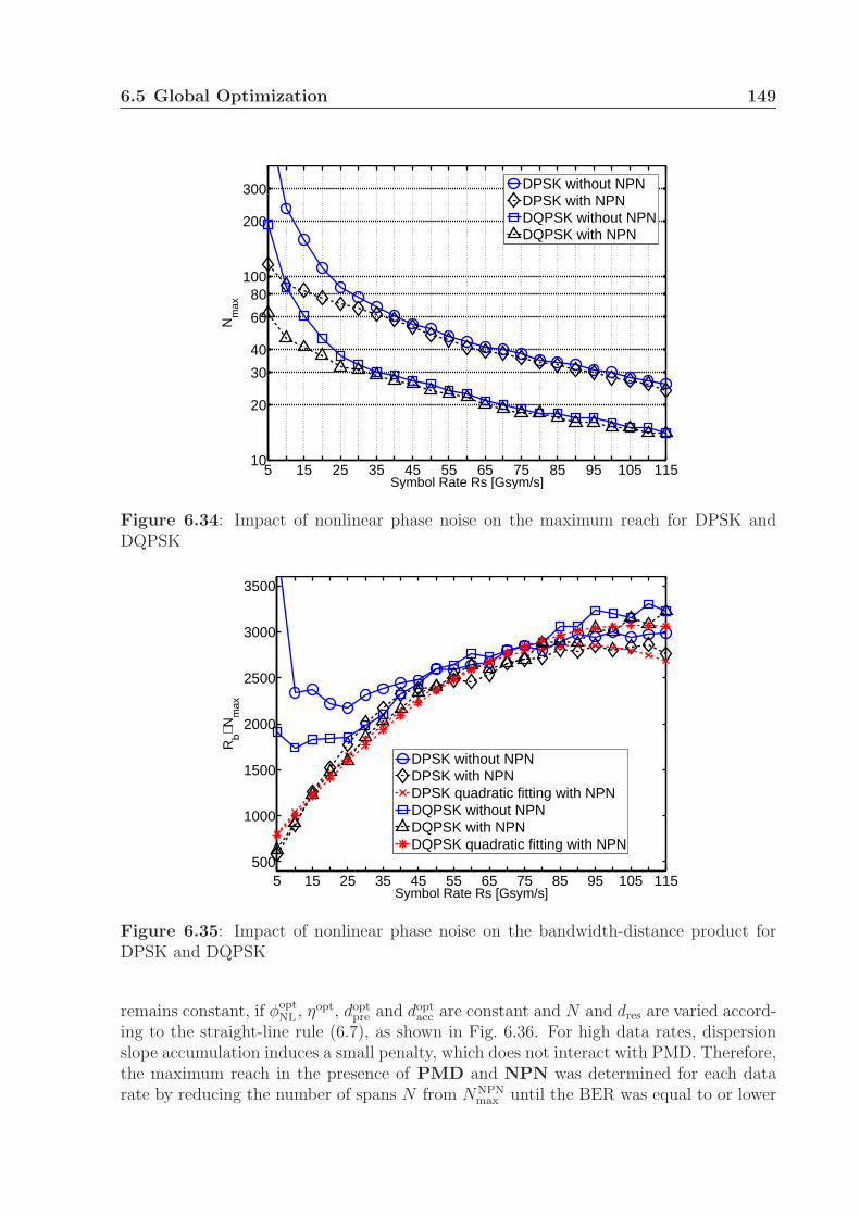
6.5 Global Optimization 149
5 15 25 35 45 55 65 75 85 95 105 11510
20
30
40
60
80100
200
300
Symbol Rate Rs [Gsym/s]
Nm
ax
DPSK without NPNDPSK with NPNDQPSK without NPNDQPSK with NPN
Figure 6.34: Impact of nonlinear phase noise on the maximum reach for DPSK andDQPSK
5 15 25 35 45 55 65 75 85 95 105 115500
1000
1500
2000
2500
3000
3500
Symbol Rate Rs [Gsym/s]
Rb⋅ N
max
DPSK without NPNDPSK with NPNDPSK quadratic fitting with NPNDQPSK without NPNDQPSK with NPNDQPSK quadratic fitting with NPN
Figure 6.35: Impact of nonlinear phase noise on the bandwidth-distance product forDPSK and DQPSK
remains constant, if φoptNL , ηopt, dopt
pre and doptacc are constant and N and dres are varied accord-
ing to the straight-line rule (6.7), as shown in Fig. 6.36. For high data rates, dispersionslope accumulation induces a small penalty, which does not interact with PMD. Therefore,the maximum reach in the presence of PMD and NPN was determined for each datarate by reducing the number of spans N from NNPN
max until the BER was equal to or lower
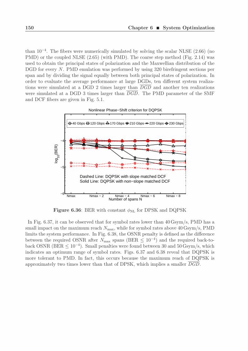
150 Chapter 6 ¥ System Optimization
than 10−4. The fibers were numerically simulated by solving the scalar NLSE (2.66) (noPMD) or the coupled NLSE (2.65) (with PMD). The coarse step method (Fig. 2.14) wasused to obtain the principal states of polarization and the Maxwellian distribution of theDGD for every N . PMD emulation was performed by using 320 birefringent sections perspan and by dividing the signal equally between both principal states of polarization. Inorder to evaluate the average performance at large DGDs, ten different system realiza-tions were simulated at a DGD 2 times larger than DGD and another ten realizationswere simulated at a DGD 3 times larger than DGD . The PMD parameter of the SMFand DCF fibers are given in Fig. 5.1.
Nmax Nmax − 2 Nmax − 4 Nmax − 6 Nmax − 8−6
−5
−4
Number of spans N
log 10
(BE
R)
Nonlinear Phase−Shift criterion for DQPSK
40 Gbps 120 Gbps 170 Gbps 210 Gbps 220 Gbps 230 Gbps
Dashed Line: DQPSK with slope matched DCFSolid Line: DQPSK with non−slope matched DCF
Figure 6.36: BER with constant φNL for DPSK and DQPSK
In Fig. 6.37, it can be observed that for symbol rates lower than 40 Gsym/s, PMD has asmall impact on the maximum reach Nmax, while for symbol rates above 40 Gsym/s, PMDlimits the system performance. In Fig. 6.38, the OSNR penalty is defined as the differencebetween the required OSNR after Nmax spans (BER ≤ 10−4) and the required back-to-back OSNR (BER ≤ 10−4). Small penalties were found between 30 and 50 Gsym/s, whichindicates an optimum range of symbol rates. Figs. 6.37 and 6.38 reveal that DQPSK ismore tolerant to PMD. In fact, this occurs because the maximum reach of DQPSK isapproximately two times lower than that of DPSK, which implies a smaller DGD .
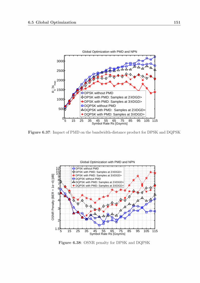
6.5 Global Optimization 151
5 15 25 35 45 55 65 75 85 95 105 1150
500
1000
1500
2000
2500
3000
Symbol Rate Rs [Gsym/s]
Rb⋅ N
max
Global Optimization with PMD and NPN
DPSK without PMDDPSK with PMD: Samples at 2⋅<DGD>DPSK with PMD: Samples at 3⋅<DGD>DQPSK without PMDDQPSK with PMD: Samples at 2⋅<DGD>DQPSK with PMD: Samples at 3⋅<DGD>
Figure 6.37: Impact of PMD on the bandwidth-distance product for DPSK and DQPSK
5 15 25 35 45 55 65 75 85 95 105 1151.5
2
3
4
5
6789
101112
Symbol Rate Rs [Gsym/s]
Global Optimization with PMD and NPN
OS
NR
Pen
alty
(B
ER
= 1
e−4)
[dB
]
DPSK without PMDDPSK with PMD: Samples at 2⋅<DGD>DPSK with PMD: Samples at 3⋅<DGD>DQPSK without PMDDQPSK with PMD: Samples at 2⋅<DGD>DQPSK with PMD: Samples at 3⋅<DGD>
Figure 6.38: OSNR penalty for DPSK and DQPSK
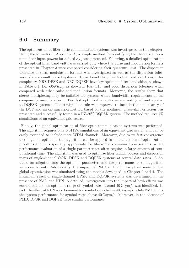
152 Chapter 6 ¥ System Optimization
6.6 Summary
The optimization of fiber-optic communication systems was investigated in this chapter.Using the formulas in Appendix A, a simple method for identifying the theoretical opti-mum fiber input powers for a fixed φNL was presented. Following, a detailed optimizationof the optical filter bandwidth was carried out, where the pulse and modulation formatspresented in Chapter 3 were compared considering their quantum limit. The dispersiontolerance of these modulation formats was investigated as well as the dispersion toler-ance of stereo multiplexed systems. It was found that, besides their reduced transmittercomplexity, NRZ-DPSK and NRZ-DQPSK have low optimum filter bandwidth, as shownin Table 6.1, low OSNRreq, as shown in Fig. 4.10, and good dispersion tolerance whencompared with other pulse and modulation formats. Moreover, the results show thatstereo multiplexing may be suitable for systems where bandwidth requirements of thecomponents are of concern. Two fast optimization rules were investigated and appliedto DQPSK systems. The straight-line rule was improved to include the nonlinearity ofthe DCF and an optimization method based on the nonlinear phase-shift criterion waspresented and successfully tested in a RZ-50% DQPSK system. The method requires 7%simulations of an equivalent grid search.
Finally, the global optimization of fiber-optic communication systems was performed.The algorithm requires only 0.0115% simulations of an equivalent grid search and can beeasily extended to include more WDM channels. Moreover, due to its fast convergenceto the global optimum, the algorithm can be applied to different kinds of optimizationproblems and it is specially appropriate for fiber-optic communication systems, whereperformance evaluation of a single parameter set often requires a large amount of com-putational time. The algorithm was used to optimize fiber launch powers and dispersionmaps of single-channel OOK, DPSK and DQPSK systems at several data rates. A de-tailed investigation into the optimum parameters and the performance of the algorithmwere carried out. Additionally, the impact of PMD and nonlinear phase noise on theglobal optimization was simulated using the models developed in Chapter 2 and 4. Themaximum reach of single-channel DPSK and DQPSK systems was determined in thepresence of PMD and NPN. A detailed investigation into the impact of both effects wascarried out and an optimum range of symbol rates around 40 Gsym/s was identified. Infact, the effect of NPN was dominant for symbol rates below 40 Gsym/s, while PMD limitsthe system performance for symbol rates above 40 Gsym/s. Moreover, in the absence ofPMD, DPSK and DQPSK have similar performance.
7Conclusions
This work dealt with the development of numerical models and algorithms, which enablethe fast and accurate simulation and optimization of fiber-optic communication systemsusing advanced modulation formats. The focus was put on systems using direct-detectionand phase-shift keying (PSK), OOK and a combination of both as modulation formats.The main contributions of this thesis can be summarized as follows:
• In Chapter 2, theoretical and practical aspects of the components involved in thedesign and simulation of a fiber-optic communication system were discussed andseveral equations were derived. Electrical signals were generated using pulse shapingand multi-level pseudo-random sequences obtained by proper decimation of binarysequences or through Galois Field theory. The Laser was shown to be the mostappropriate source for long-haul systems due to its small linewidth.
• The propagation equations of the light in a single-mode fiber and their numericalsolution were derived considering several linear and nonlinear effects. Three meth-ods were used in the simulations: the split-step (1), the coarse-step (2) and thenonlinear coarse-step (3) methods. They can accurately reproduce the propagationof optical signals in practical fiber-optic communication systems. The use of oneof these methods depends on the dominant impairment, i.e., fiber nonlinearity (1),birefringence (2) or both impairments (3). In absence of fiber nonlinearity andbirefringence, a closed-form solution is available.
• The theory and operation of Mach-Zehnder modulators (MZM) was described, aswell as its role in the generation of advanced modulation formats. In fact, anymodulation format can be generated using Mach-Zehnder and phase modulators. In

154 Chapter 7 ¥ Conclusions
order to relax the bandwidth requirements of the components a stereo multiplexingtechnique for dual-carrier transmission was also analyzed.
• At the receiver side, photodiodes and delay interferometers were used to recover theinformation encoded in the phase and amplitude. It was shown that the decisioncurrents can be written as a double integral of a Hermitian kernel and the receivedoptical signal. The Hermitian kernel describes the receiver structure and was derivedfor each modulation format as well as for stereo multiplexing. The Hermitian kernelis an essential part in the evaluation of the BER.
• An algorithm for evaluating the BER in the presence of nonlinear phase noise (NPN)was presented. It is based on the Karhunen-Loeve (KL) series expansion and ona system transmission matrix W(f). First, a standard Karhunen-Loeve methodwas derived and validated using analytical formulas (Appendix A). Following, theextended Karhunen-Loeve method was derived and validated through an experi-ment, where the effect of dispersion on the NPN was shown to improve the systemperformance when NPN is the dominant impairment. Finally, the standard andmulti-canonical Monte Carlo methods were derived and a strategy for noise gen-eration in frequency domain was presented in order to speed up the simulations.Therefore, five methods for evaluating the BER were extensively discussed and mu-tually validated.
• Among all investigated modulation formats, DPSK has shown the best back-to-backperformance, followed by DQPSK for a fixed data rate Rb. Moreover, besides theirreduced transmitter complexity, NRZ-DPSK and NRZ-DQPSK have low optimumfilter bandwidth, as shown in Table 6.1, low OSNRreq, as shown in Fig. 4.10, andgood dispersion tolerance when compared with other pulse and modulation for-mats. Additionally, the performance of stereo multiplexed systems shows that itmay be suitable for systems where bandwidth requirements of the components areof concern.
• Three optimization strategies for fiber-optic long-haul communication systems wereinvestigated. First, a simple method for identifying the theoretical optimum fiberinput powers for a fixed φNL was presented. Then, two fast optimization rules wereinvestigated and applied to DQPSK systems. The straight-line rule was improvedto include the nonlinearity of the DCF and an optimization method based on thenonlinear phase-shift criterion was presented and successfully tested in a RZ-50%DQPSK system. The method requires 7% simulations of an equivalent grid search.
• Finally, a global optimization algorithm was developed in order to speed up theoptimization process. The algorithm requires only 0.0115% simulations of an equiv-alent grid search. The algorithm was used first to optimize fiber launch powersand dispersion map of single-channel OOK, DPSK and DQPSK systems at severaldata rates. Following, the impact of PMD and nonlinear phase noise were evaluatedusing almost all numerical methods derived in this thesis. An optimum range ofsymbol rates around 40 Gsym/s was identified. It was observed that the effect of
155
NPN was dominant for symbol rates below 40 Gsym/s, while PMD limits the systemperformance for symbol rates above 40 Gsym/s. Moreover, in the absence of PMD,DPSK and DQPSK have similar performance.
During this work, several interesting problems were left for future investigation. Someof them are listed below:
• Coherent detection with polarization multiplexing and digital signal processing isa promising technique to further improve the system performance. The evaluationof the BER in these systems is normally performed by the standard Monte Carlomethod. Therefore, fast optimization rules and global optimization algorithms canspeed up the simulation and design of fiber-optic communication systems usingcoherent detection.
• Most commercial systems employ WDM to transmit information at high data rates.A natural extension of the topics treated in this thesis is the inclusion of neigh-boring channels. Since each channel uses a different Laser source, their phases arenot matched, which reduces the crosstalk after detection and the impact of nonlin-ear effects. Additionally, the evolution of the polarization state of each channel isdifferent, which further reduces the impact of inter-channel nonlinear effects. There-fore, a statistical treatment can be done in order to evaluate the average impact ofneighboring channels.
• The global optimization algorithm presented in this thesis approximates the objec-tive function over a bounded space by a set of simplexes. Alternatively, radial basisfunctions can be used to approximate the objective function in order to furtherimprove the performance of the algorithm.
• Several fiber-optic communication systems use forward-error correction (FEC) codesin order to benefit from gains up to 10 dB. These codes are usually designed forsignals corrupted by AWGN noise, which may not be the case of the optical receivednoise. Thus, optimization of FEC codes for a given nonlinear system or systemoptimization using a standard FEC may lead to large improvements in performance.Moreover, multi-canonical Monte Carlo methods may be used in these systems todetect events which lead to complete system failure.
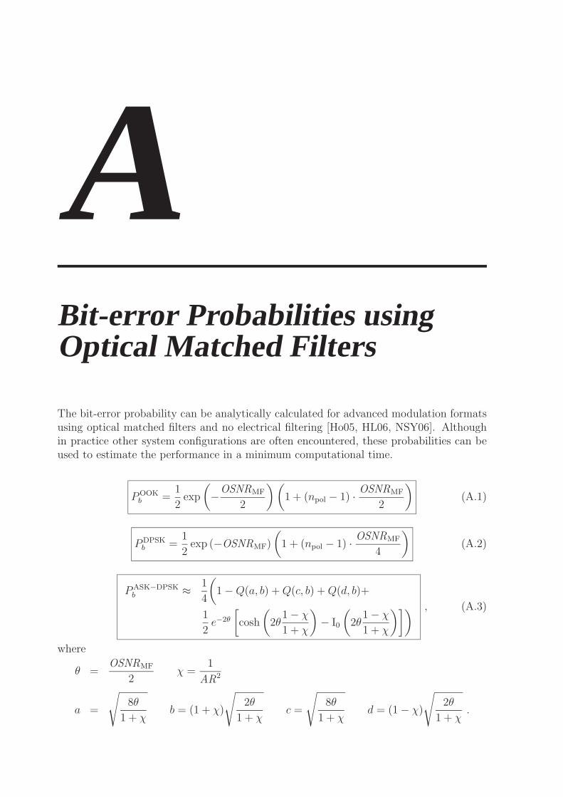
ABit-error Probabilities usingOptical Matched Filters
The bit-error probability can be analytically calculated for advanced modulation formatsusing optical matched filters and no electrical filtering [Ho05, HL06, NSY06]. Althoughin practice other system configurations are often encountered, these probabilities can beused to estimate the performance in a minimum computational time.
POOKb =
1
2exp
(−OSNRMF
2
) (1 + (npol − 1) · OSNRMF
2
)(A.1)
PDPSKb =
1
2exp (−OSNRMF)
(1 + (npol − 1) · OSNRMF
4
)(A.2)
PASK−DPSKb ≈ 1
4
(1 − Q(a, b) + Q(c, b) + Q(d, b)+
1
2e−2θ
[cosh
(2θ
1 − χ
1 + χ
)− I0
(2θ
1 − χ
1 + χ
)]) , (A.3)
where
θ =OSNRMF
2χ =
1
AR2
a =
√8θ
1 + χb = (1 + χ)
√2θ
1 + χc =
√8θ
1 + χd = (1 − χ)
√2θ
1 + χ.
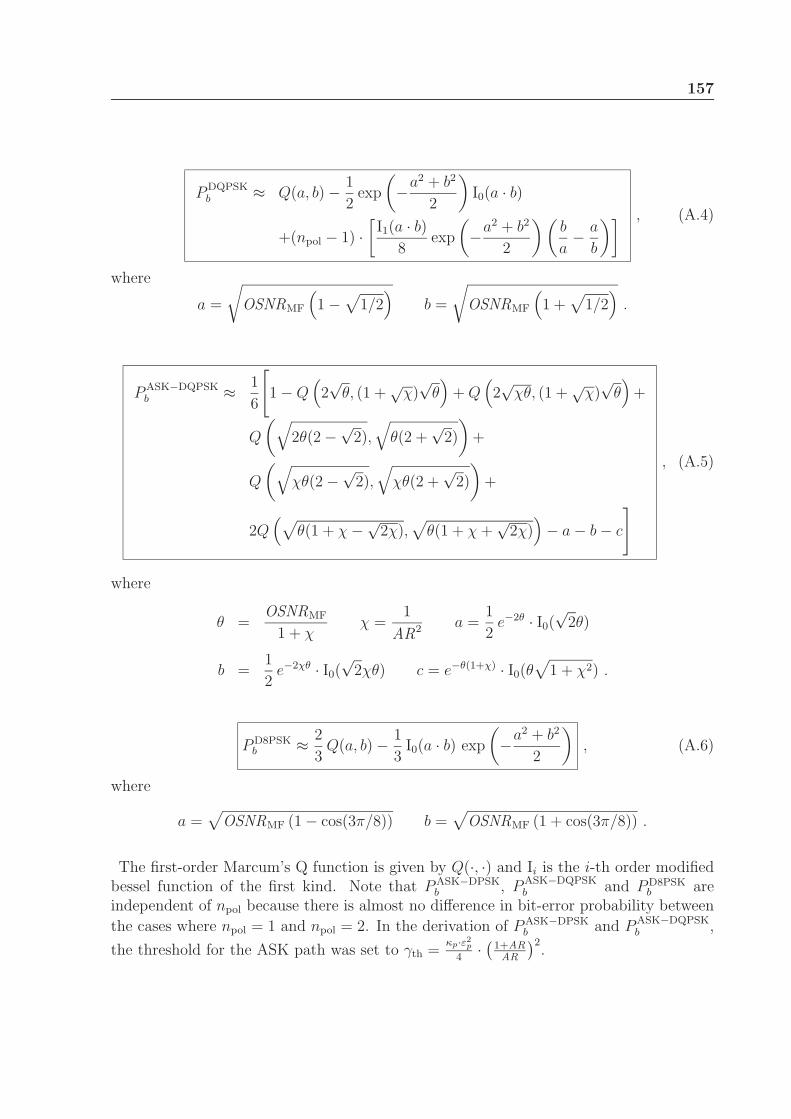
157
PDQPSKb ≈ Q(a, b) − 1
2exp
(−a2 + b2
2
)I0(a · b)
+(npol − 1) ·[I1(a · b)
8exp
(−a2 + b2
2
) (b
a− a
b
)] , (A.4)
where
a =
√OSNRMF
(1 −
√1/2
)b =
√OSNRMF
(1 +
√1/2
).
PASK−DQPSKb ≈ 1
6
[1 − Q
(2√
θ, (1 +√
χ)√
θ)
+ Q(2√
χθ, (1 +√
χ)√
θ)
+
Q
(√2θ(2 −
√2),
√θ(2 +
√2)
)+
Q
(√χθ(2 −
√2),
√χθ(2 +
√2)
)+
2Q(√
θ(1 + χ −√2χ),
√θ(1 + χ +
√2χ)
)− a − b − c
]
, (A.5)
where
θ =OSNRMF
1 + χχ =
1
AR2 a =1
2e−2θ · I0(
√2θ)
b =1
2e−2χθ · I0(
√2χθ) c = e−θ(1+χ) · I0(θ
√1 + χ2) .
PD8PSKb ≈ 2
3Q(a, b) − 1
3I0(a · b) exp
(−a2 + b2
2
), (A.6)
where
a =√
OSNRMF (1 − cos(3π/8)) b =√
OSNRMF (1 + cos(3π/8)) .
The first-order Marcum’s Q function is given by Q(·, ·) and Ii is the i-th order modifiedbessel function of the first kind. Note that PASK−DPSK
b , PASK−DQPSKb and PD8PSK
b areindependent of npol because there is almost no difference in bit-error probability between
the cases where npol = 1 and npol = 2. In the derivation of PASK−DPSKb and PASK−DQPSK
b ,
the threshold for the ASK path was set to γth =κp·ε2
p
4·(
1+AR
AR
)2.
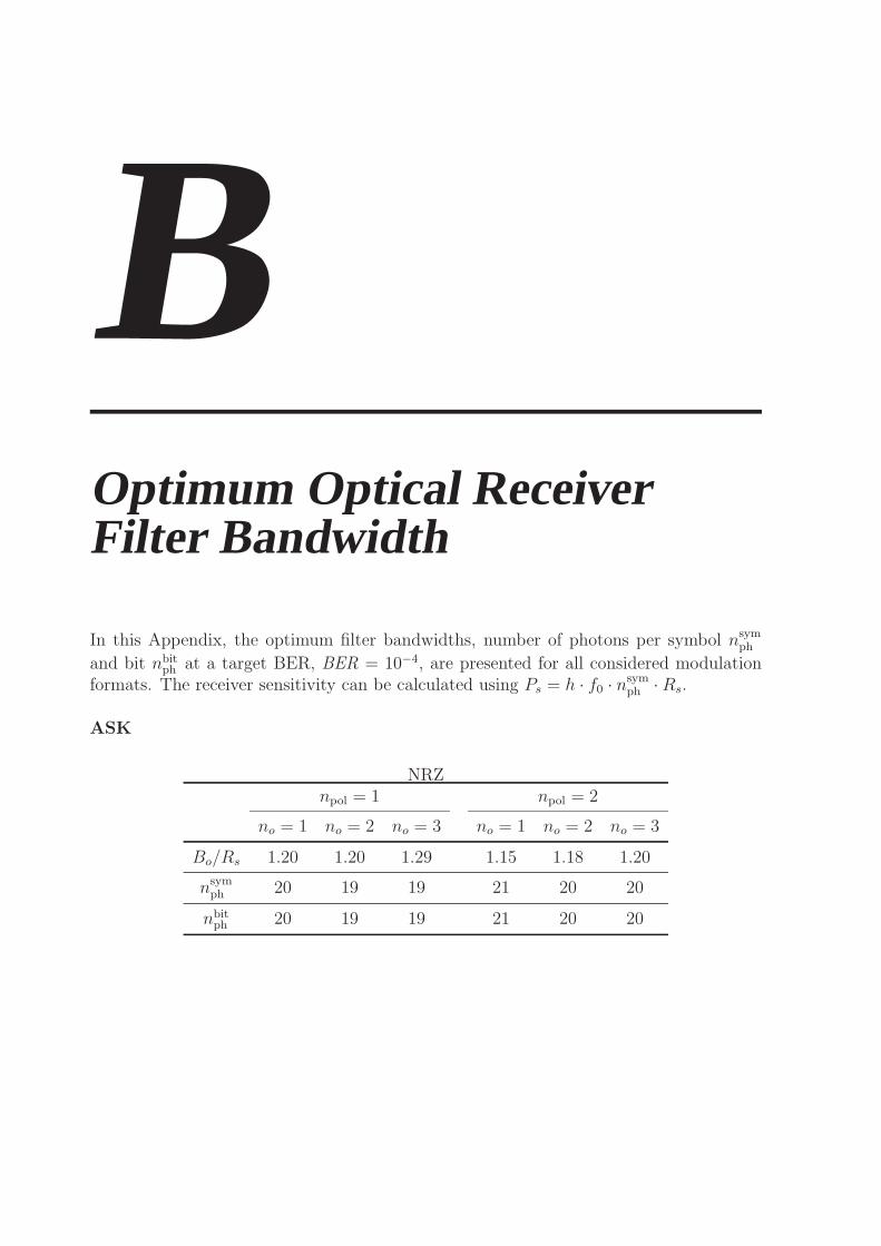
BOptimum Optical ReceiverFilter Bandwidth
In this Appendix, the optimum filter bandwidths, number of photons per symbol nsymph
and bit nbitph at a target BER, BER = 10−4, are presented for all considered modulation
formats. The receiver sensitivity can be calculated using Ps = h · f0 · nsymph · Rs.
ASK
NRZnpol = 1 npol = 2
no = 1 no = 2 no = 3 no = 1 no = 2 no = 3
Bo/Rs 1.20 1.20 1.29 1.15 1.18 1.20
nsymph 20 19 19 21 20 20
nbitph 20 19 19 21 20 20
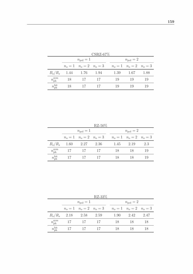
159
CSRZ-67%
npol = 1 npol = 2
no = 1 no = 2 no = 3 no = 1 no = 2 no = 3
Bo/Rs 1.44 1.76 1.94 1.39 1.67 1.88
nsymph 18 17 17 19 19 19
nbitph 18 17 17 19 19 19
RZ-50%
npol = 1 npol = 2
no = 1 no = 2 no = 3 no = 1 no = 2 no = 3
Bo/Rs 1.60 2.27 2.36 1.45 2.19 2.3
nsymph 17 17 17 18 18 19
nbitph 17 17 17 18 18 19
RZ-33%
npol = 1 npol = 2
no = 1 no = 2 no = 3 no = 1 no = 2 no = 3
Bo/Rs 2.18 2.58 2.59 1.90 2.42 2.47
nsymph 17 17 17 18 18 18
nbitph 17 17 17 18 18 18

160 Appendix B ¥ Optimum Optical Receiver Filter Bandwidth
DPSK
NRZnpol = 1 npol = 2
no = 1 no = 2 no = 3 no = 1 no = 2 no = 3
Bo/Rs 1.12 1.22 1.29 1.09 1.21 1.28
nsymph 10 9 10 11 11 11
nbitph 10 9 10 11 11 11
CSRZ-67%
npol = 1 npol = 2
no = 1 no = 2 no = 3 no = 1 no = 2 no = 3
Bo/Rs 1.26 1.70 1.90 1.24 1.67 1.88
nsymph 9 9 9 11 11 11
nbitph 9 9 9 11 11 11
RZ-50%
npol = 1 npol = 2
no = 1 no = 2 no = 3 no = 1 no = 2 no = 3
Bo/Rs 1.56 1.99 2.12 1.53 1.96 2.09
nsymph 9 9 9 10 11 11
nbitph 9 9 9 10 11 11
RZ-33%
npol = 1 npol = 2
no = 1 no = 2 no = 3 no = 1 no = 2 no = 3
Bo/Rs 1.94 2.34 2.49 1.88 2.28 2.42
nsymph 9 9 9 10 11 11
nbitph 9 9 9 10 11 11

161
ASK-DPSK
NRZnpol = 1 npol = 2
no = 1 no = 2 no = 3 no = 1 no = 2 no = 3
Bo/Rs 1.70 1.42 1.53 1.60 1.42 1.47
nsymph 47 42 44 50 45 46
nbitph 24 21 22 25 23 23
CSRZ-67%
npol = 1 npol = 2
no = 1 no = 2 no = 3 no = 1 no = 2 no = 3
Bo/Rs 1.38 2.10 2.22 1.36 1.97 2.15
nsymph 38 38 40 41 43 43
nbitph 19 19 20 21 22 22
RZ-50%
npol = 1 npol = 2
no = 1 no = 2 no = 3 no = 1 no = 2 no = 3
Bo/Rs 1.61 2.19 2.22 1.56 2.10 2.16
nsymph 37 37 37 40 40 41
nbitph 19 19 19 20 20 22
RZ-33%
npol = 1 npol = 2
no = 1 no = 2 no = 3 no = 1 no = 2 no = 3
Bo/Rs 2.04 2.43 2.60 1.92 2.36 2.48
nsymph 37 37 37 40 40 40
nbitph 19 19 19 20 20 20
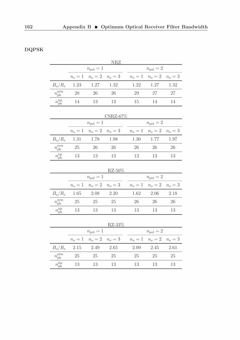
162 Appendix B ¥ Optimum Optical Receiver Filter Bandwidth
DQPSK
NRZnpol = 1 npol = 2
no = 1 no = 2 no = 3 no = 1 no = 2 no = 3
Bo/Rs 1.23 1.27 1.32 1.22 1.27 1.32
nsymph 28 26 26 29 27 27
nbitph 14 13 13 15 14 14
CSRZ-67%
npol = 1 npol = 2
no = 1 no = 2 no = 3 no = 1 no = 2 no = 3
Bo/Rs 1.31 1.78 1.98 1.30 1.77 1.97
nsymph 25 26 26 26 26 26
nbitph 13 13 13 13 13 13
RZ-50%
npol = 1 npol = 2
no = 1 no = 2 no = 3 no = 1 no = 2 no = 3
Bo/Rs 1.65 2.08 2.20 1.62 2.06 2.18
nsymph 25 25 25 26 26 26
nbitph 13 13 13 13 13 13
RZ-33%
npol = 1 npol = 2
no = 1 no = 2 no = 3 no = 1 no = 2 no = 3
Bo/Rs 2.15 2.49 2.65 2.09 2.45 2.61
nsymph 25 25 25 25 25 25
nbitph 13 13 13 13 13 13

163
ASK-DQPSK
NRZnpol = 1 npol = 2
no = 1 no = 2 no = 3 no = 1 no = 2 no = 3
Bo/Rs 1.71 1.31 1.24 1.70 1.31 1.25
nsymph 76 68 70 78 69 71
nbitph 26 23 24 26 23 24
CSRZ-67%
npol = 1 npol = 2
no = 1 no = 2 no = 3 no = 1 no = 2 no = 3
Bo/Rs 1.42 2.41 2.50 1.39 2.40 2.50
nsymph 62 67 67 63 69 68
nbitph 21 23 23 21 23 23
RZ-50%
npol = 1 npol = 2
no = 1 no = 2 no = 3 no = 1 no = 2 no = 3
Bo/Rs 1.74 2.22 2.22 1.72 2.20 2.21
nsymph 60 60 60 61 61 61
nbitph 20 20 20 21 21 21
RZ-33%
npol = 1 npol = 2
no = 1 no = 2 no = 3 no = 1 no = 2 no = 3
Bo/Rs 2.20 2.47 2.90 2.15 2.42 2.86
nsymph 59 59 60 60 60 61
nbitph 20 20 20 20 20 21
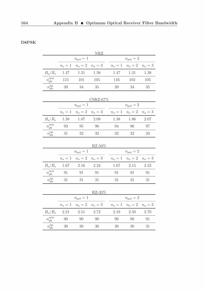
164 Appendix B ¥ Optimum Optical Receiver Filter Bandwidth
D8PSK
NRZnpol = 1 npol = 2
no = 1 no = 2 no = 3 no = 1 no = 2 no = 3
Bo/Rs 1.47 1.31 1.38 1.47 1.31 1.38
nsymph 115 101 105 116 102 105
nbitph 39 34 35 39 34 35
CSRZ-67%
npol = 1 npol = 2
no = 1 no = 2 no = 3 no = 1 no = 2 no = 3
Bo/Rs 1.38 1.87 2.08 1.38 1.86 2.07
nsymph 93 95 96 94 96 97
nbitph 31 32 32 32 32 33
RZ-50%
npol = 1 npol = 2
no = 1 no = 2 no = 3 no = 1 no = 2 no = 3
Bo/Rs 1.67 2.16 2.24 1.67 2.15 2.23
nsymph 91 91 91 91 91 91
nbitph 31 31 31 31 31 31
RZ-33%
npol = 1 npol = 2
no = 1 no = 2 no = 3 no = 1 no = 2 no = 3
Bo/Rs 2.21 2.51 2.72 2.19 2.50 2.70
nsymph 90 90 90 90 90 91
nbitph 30 30 30 30 30 31

CNotation, Symbols andAbbreviations
Acronyms
AR Amplitude ratioASE Amplified spontaneous emissionASK Amplitude shift keyingAWG Array waveguide gratingAWGN Additive white gaussian noiseBER Bit-error rateCD Chromatic dispersionCSM Coarse-step methodCSRZ Carrier-suppressed return-to-zeroCRZ Chirped return-to-zeroCW Continuous waveD8PSK Differential 8-phase-shift keyingDCF Dispersion compensating fiberDFT Discrete Fourier transformDGD Differential group delayDPSK Differential phase-shift keyingDQPSK Differential quadrature phase-shift keyingDSP Digital signal processing or processorEAM Electro-absorption modulatorEDFA Erbium doped fiber amplifier
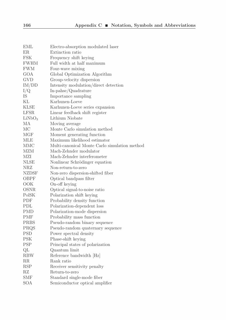
166 Appendix C ¥ Notation, Symbols and Abbreviations
EML Electro-absorption modulated laserER Extinction ratioFSK Frequency shift keyingFWHM Full width at half maximumFWM Four-wave mixingGOA Global Optimization AlgorithmGVD Group-velocity dispersionIM/DD Intensity modulation/direct detectionI/Q In-pahse/QuadratureIS Importance samplingKL Karhunen-LoeveKLSE Karhunen-Loeve series expansionLFSR Linear feedback shift registerLiNbO3 Lithium NiobateMA Moving averageMC Monte Carlo simulation methodMGF Moment generating functionMLE Maximum likelihood estimatorMMC Multi-canonical Monte Carlo simulation methodMZM Mach-Zehnder modulatorMZI Mach-Zehnder interferometerNLSE Nonlinear Schrodinger equationNRZ Non-return-to-zeroNZDSF Non-zero dispersion-shifted fiberOBPF Optical bandpass filterOOK On-off keyingOSNR Optical signal-to-noise ratioPolSK Polarization shift keyingPDF Probability density functionPDL Polarization-dependent lossPMD Polarization-mode dispersionPMF Probability mass functionPRBS Pseudo-random binary sequencePRQS Pseudo-random quaternary sequencePSD Power spectral densityPSK Phase-shift keyingPSP Principal states of polarizationQL Quantum limitRBW Reference bandwidth [Hz]RR Rank ratioRSP Receiver sensitivity penaltyRZ Return-to-zeroSMF Standard single-mode fiberSOA Semiconductor optical amplifier

167
SPM Self-phase modulationSSFM Split-step fourier methodSRS Stimulated Raman scatteringTi : LiNbO3 Titanium-diffused Lithium NiobateWDM Wavelength division multiplexing or multiplexer
Mathematical Notation and Functions
(·)∗ Conjugate of argument(·)−1 Inverse of a matrix(·)T Transpose of a vector or matrix(·)∗ Complex conjugate(·)H Complex conjugate and transpose of a vector or matrix|v| Absolute value or cardinality of argument‖ · ‖ Euclidean distance⌊·⌋ Floor function⌈·⌉ Ceiling function∗ Convolutional operator⊕ Exclusive-or binary operator(·) Binary not operatorΓ(·) Gamma functionδ(·) Dirac delta functionδab Kronecker delta functionE· Expectation of a random variableerfc(·) Complementary error functionF· Direct Fourier transformF−1· Inverse Fourier transformIm· Imaginary part of argumentIi i-th order modified bessel function of the first kindln(·) Natural logarithmPr· Probability of an eventQ(a, b) First-order Marcum’s Q functionrect(·) Rectangular functionRe· Real part of argumentu(·) Unit step functionVar· Variance of a random variable
Greek Symbols
α Fiber attenuation [1/m]αRC Roll-off factor in the electrical signal generation
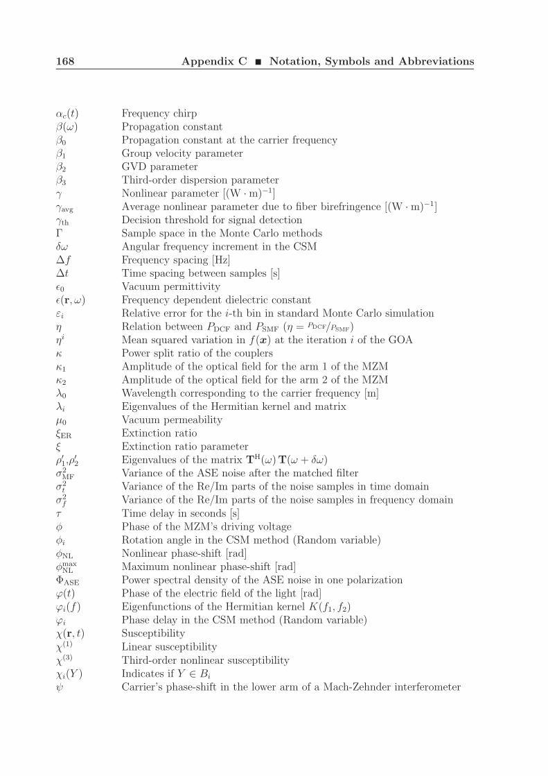
168 Appendix C ¥ Notation, Symbols and Abbreviations
αc(t) Frequency chirpβ(ω) Propagation constantβ0 Propagation constant at the carrier frequencyβ1 Group velocity parameterβ2 GVD parameterβ3 Third-order dispersion parameterγ Nonlinear parameter [(W · m)−1]γavg Average nonlinear parameter due to fiber birefringence [(W · m)−1]γth Decision threshold for signal detectionΓ Sample space in the Monte Carlo methodsδω Angular frequency increment in the CSM∆f Frequency spacing [Hz]∆t Time spacing between samples [s]ǫ0 Vacuum permittivityǫ(r, ω) Frequency dependent dielectric constantεi Relative error for the i-th bin in standard Monte Carlo simulationη Relation between PDCF and PSMF (η = PDCF/PSMF)ηi Mean squared variation in f(x) at the iteration i of the GOAκ Power split ratio of the couplersκ1 Amplitude of the optical field for the arm 1 of the MZMκ2 Amplitude of the optical field for the arm 2 of the MZMλ0 Wavelength corresponding to the carrier frequency [m]λi Eigenvalues of the Hermitian kernel and matrixµ0 Vacuum permeabilityξER Extinction ratioξ Extinction ratio parameterρ′
1,ρ′2 Eigenvalues of the matrix TH(ω)T(ω + δω)
σ2MF Variance of the ASE noise after the matched filter
σ2t Variance of the Re/Im parts of the noise samples in time domain
σ2f Variance of the Re/Im parts of the noise samples in frequency domain
τ Time delay in seconds [s]φ Phase of the MZM’s driving voltageφi Rotation angle in the CSM method (Random variable)φNL Nonlinear phase-shift [rad]φmax
NL Maximum nonlinear phase-shift [rad]ΦASE Power spectral density of the ASE noise in one polarizationϕ(t) Phase of the electric field of the light [rad]ϕi(f) Eigenfunctions of the Hermitian kernel K(f1, f2)ϕi Phase delay in the CSM method (Random variable)χ(r, t) Susceptibilityχ(1) Linear susceptibilityχ(3) Third-order nonlinear susceptibilityχi(Y ) Indicates if Y ∈ Bi
ψ Carrier’s phase-shift in the lower arm of a Mach-Zehnder interferometer

169
ΨY (s) MGF of the random variable Yω Angular frequency in radian [rad/s]ω0 Carrier frequency [rad/s]
Roman Symbols
ai Information sequenceai(t) Electrical signal representing the information sequence ai
a(z, t) Noise in the linearization of the NLSE. a(z, t) = ap(z, t) + jaq(z, t)Aeff Effective core area
A(z, t) Slowly varying amplitude of the electric field [√
W]AR Amplitude ratiobi(t) Filtered electrical signal representing the information sequence ai
B(z, t) Slowly varying amplitude of the electric field [V/m]B Magnetic flux densityBe Electrical receiver filter bandwidth [Hz]Bo Optical receiver filter bandwidth [Hz]Bo,eff Effective optical filter bandwidth [Hz]Bi Interval corresponding to the i-th binBW Simulation bandwidth [Hz]c Speed of light in vacuum [m/s]Ch1, Ch2 Channel 1 and 2 in stereo multiplexingd Duty cycle of the optical pulses p(t)di(t) Electrical signal representing the differential encoding of ai
dacc Accumulated amount of dispersion at the end of the link [s/m]dpos Amount of post-compensation of the dispersion [s/m]dpre Amount of pre-compensation of the dispersion [s/m]dres Residual dispersion per span [s/m]D Dispersion parameter [s/m/m]DPMD PMD parameter [s/
√m]
D Electric flux densityD0 Anti-diagonal matrix
D(ω) Differential operator in the frequency domainDPMD PMD parameter of the fiberDGD Differential group delay due to fiber birefringenceDGD Average DGD
D(ω) Delay matrix in the coarse-step methode Euler’s numberek Error event of the k-th bite Sampled electric field vector of the lighte Unit vector representing the state of polarization of the electric fieldE Electric field vector
E(z, t) Electric field of the light [√
W]

170 Appendix C ¥ Notation, Symbols and Abbreviations
E1 Ground state energyE2 Excited state energyEph Photon energy [J]f Frequency in Herz [Hz]f Frequency vector of length 2Mf0 Carrier frequency in Herz [Hz]fp Frequency of the MZM’s driving voltageFn EDFA noise figureF (x, y) Transversal field distribution of the fundamental fiber modegi Tap coefficients of a LFSRG EDFA gainG(X) Generator polynomialGi(z, ω) PSD matrix of the ASE noise after i spansh Planck’ constantH Magnetic field vectorHi Transfer matrix of a symmetric filterHo(f) Transfer function of the optical filterHe(f) Transfer function of the electrical filterHRC(f) Transfer function of the raised cosine filterI(t) Electric current after demodulationI Identity matrixj Complex number
√−1
k0 Free-space wave number [rad/m]K(f1, f2) Hermitian kernelK Hermitian matrixL Fiber length [m]Leff Effective fiber length [m]Lc Correlation length of the fiber [m]2M Total number of frequency samplesM Fiber transmission matrix or induced magnetic polarizationn(z, ω) 2 × 1 noise vector containing the real and imaginary parts of a(z, ω)ns Number of shift registers in a LFSRno Gaussian optical filter ordernpol Number of polarizations containing noisenph Minimum number of photons required for a target BERn(z, t) Noise part of the electric fieldn2 Nonlinear refractive indexn(ω) Frequency dependent refractive index
N(z, t) Nonlinear operator in time domainN Number of spansNb Number of bins in the Monte Carlo methodsNi Number of samples that fall in the i-th binN Set of natural numbersNCSM Number of small birefringent segments

171
Ns Number of samples in the standard MC and MMC methodsNsec Number of sections of the fiber transmission matrixNseq Length of the information sequence ai
Nsym Number of samples per symbolNw Size of the window for the evaluation of Pb
OSNR Optical signal-to-noise ratio over a reference bandwidthOSNRMF Optical signal-to-noise ratio after the matched filterpi
in Input principal state of polarization vectorp(t) Optical pulse generated by the pulse carverpX(x), pY (y) Probability density function of the random variable X and YPASE ASE noise powerPb Bit-error probabilityP0 Peak power of the signal s(z, t)PY (Bi) Probability that a sample falls in the i-th binP Induced electric polarization (different from light polarization)Pin Matrix containing the input PSP’sPout Matrix containing the output PSP’sqi Eigenvectors of the Hermitian matrixr Number of bits per symbolr Spatial coordinateR Photodiode responsivity [A/W]R Set of real numbersRb Data rate [Gbit/s]Rs Symbol rate [Gsym/s]RBW Reference bandwidth [Hz]R(ϕi, φi) Rotation matrix in the coarse-step methods(z, t) Signal part of A(z, t)s(z, ω) 2 × 1 signal vector containing the real and imaginary parts of s(z, ω)S Slope parameter [s/m2/m]t Time in seconds [s]Ts Symbol duration [s]TFWHM Full pulse width at half maximum of the pulse power [s]
T(ω) Transfer matrix of the fiber in the coarse-step methodu0 Saddlepoint in evaluation of the BERv(t) Driving voltage of the MZMv1(t), v2(t) Driving voltage of each arm of a MZMvbias Bias of the MZM’s driving voltageVπ MZM’s driving voltage to produce a π phase shift [V]Vp MZM’s peak driving voltagew(x) Importance sampling weightW(f) System transmission matrix in the linearization of the NLSEx, y Polarization vectors of the lightx, y Transversal coordinatesX Random variable or generator polynomial variable

172 Appendix C ¥ Notation, Symbols and Abbreviations
X Random vectorY Random variablez Longitudinal coordinate variable [m]dz Stepsize in the numerical solution of the propagation equation [m]dzmax Maximum stepsize in the numerical solution of the propagation equation [m]ZF Waveguide impedance [Ω]Z Set of integer numbers

173
Bibliography
[ABF02] J. C. Antona, S. Bigo, and J. P. Faure. Nonlinear cumulated phase as acriterion to assess performance of terrestrial WDM systems. In Proc. OpticalFiber Communication Conference and Exhibit (OFC 2002), Anaheim, USA,March 2002.
[Agr02] Govind P. Agrawal. Fiber-Optic Communication Systems. John Wiley &Sons, Inc, New York, USA, 3rd edition, 2002.
[Agr05a] Govind P. Agrawal. Lightwave Technology: Components and Devices. JohnWiley & Sons, Inc, New Jersey, USA, 2005.
[Agr05b] Govind P. Agrawal. Lightwave Technology: Telecommunication Systems.John Wiley & Sons, Inc, New Jersey, USA, 2005.
[Agr06] Govind P. Agrawal. Nonlinear Fiber Optics. Academic Press, San Diego,USA, 4th edition, 2006.
[BCM+98] J. Burgemeier, A. Cords, R. Marz, C. Schaffer, and B. Stummer. A blackbox model of EDFA’s operating in WDM systems. J. Lightw. Technol.,16(7):1271–1275, July 1998.
[Ber98] B. A. Berg. Algorithmic aspects of multicanonical simulations. NuclearPhysics B Proceedings Supplements, 63:982–984, April 1998.
[Ber99] B. A. Berg. Introduction to Multicanonical Monte Carlo Simulations. ArXivCondensed Matter e-prints, September 1999.
[BN91] B. A. Berg and T. Neuhaus. Multicanonical algorithms for first order phasetransitions. Physics Letters B, 267:249–253, September 1991.
[BN92] B. A. Berg and T. Neuhaus. Multicanonical ensemble: A new approachto simulate first-order phase transitions. Physical Review Letters, 68:9–12,January 1992.
[Boy08] Robert W. Boyd. Nonlinear Optics. Academic Press, San Diego, USA, 3rdedition, 2008.
174 Bibliography
[BP04] G. Bosco and P. Poggiolini. On the Q factor inaccuracy in the performanceanalysis of optical direct-detection DPSK systems. IEEE Photon. Technol.Lett., 16(2):665–667, Feb. 2004.
[BRG+09] A. Bononi, L.A. Rusch, A. Ghazisaeidi, F. Vacondio, and N. Rossi. A FreshLook at Multicanonical Monte Carlo from a Telecom Perspective. In GlobalTelecommunications Conference, 2009. GLOBECOM 2009. IEEE, pages 1–8, nov. 2009.
[BSO08] A. Bononi, P. Serena, and A. Orlandini. A Unified Design Framework forSingle-Channel Dispersion-Managed Terrestrial Systems. J. Lightw. Tech-nol., 26(22):3617–3631, Nov. 2008.
[CGH09] L. D. Coelho, O. Gaete, and N. Hanik. An algorithm for global optimiza-tion of optical communication systems. AEU - International Journal ofElectronics and Communications, 63(7):541 – 550, 2009.
[CGS+09] L. D. Coelho, O. Gaete, E.-D. Schmidt, B. Spinnler, and N. Hanik. Globaloptimization of RZ-DPSK and RZ-DQPSK systems at various data rates.In Optical Fiber Communication Conference and Exposition (OFC 2009),San Diego, USA, March 2009.
[CGS+10] L. D. Coelho, O. Gaete, E.-D. Schmidt, B. Spinnler, and N. Hanik. Impactof PMD and Nonlinear Phase Noise on the Global Optimization of DPSKand DQPSK Systems. In Proc. Optical Fiber Communication Conferenceand Exposition (OFC 2010), San Diego, USA, March 2010.
[CH05] L. D. Coelho and N. Hanik. Higher Order Modulation Formats for High-Speed Transmission Systems. In Workshop on Optical Transmission andEqualization (WOTE 2005), pages 13–14, Shanghai, China, November 2005.
[CHH+01] C. Caspar, K. Habel, N. Heimes, M. Konitzer, M. Malach, H. Ozdem, M. Ro-hde, F. Schmidt, E. J. Bachus, and N. Hanik. Penalties through XPMcrosstalk in a switched long haul standard fiber WDM system based onnormalized transmission sections. In Proc. Optical Fiber CommunicationConference and Exhibit (OFC 2001), Anaheim, USA, March 2001.
[CHS06] L. D. Coelho, N. Hanik, and E.-D. Schmidt. Exact Numerical Evaluationof Optical Receivers Using Advanced Modulation Formats. In Proc. In-ternational Conference on Transparent Optical Networks, volume 1, pages127–131, June 2006.
[CMG+07] L. D. Coelho, L. Molle, D. Gross, N. Hanik, R. Freund, C. Caspar, andE.-D. Schmidt. Numerical and Experimental Investigation of the Effectof Dispersion on Nonlinear Phase Noise in RZ-DPSK Systems. In Proc.33rd European Conference on Optical Communication, ECOC 2007, Berlin,Germany, September 2007.
Bibliography 175
[CMG+09] L.D. Coelho, L. Molle, D. Gross, N. Hanik, R. Freund, C. Caspar, E.-D.Schmidt, and B. Spinnler. Modeling nonlinear phase noise in differentiallyphase-modulated optical communication systems. Opt. Express, 17(5):3226–3241, 2009.
[CSC06] D. O. Caplan, M. L. Stevens, and J. J. Carney. High-sensitivity multi-channel single-interferometer DPSK receiver. Opt. Express, 14(23):10984–10989, 2006.
[CSC07] D.O. Caplan, M.L. Stevens, and J.J. Carney. High-Sensitivity Demodu-lation of Multiple-Data-Rate WDM-DPSK Signals using a Single Interfer-ometer. In Proc. Optical Fiber Communication Conference and Exposition(OFC2007), Anaheim, USA, March 2007.
[CWI98] A. V. T. Cartaxo, B. Wedding, and W. Idler. Influence of fiber nonlinearityon the phase noise to intensity noise conversion in fiber transmission: the-oretical and experimental analysis. J. Lightw. Technol., 16(7):1187–1194,July 1998.
[CWI99] A. V. T. Cartaxo, B. Wedding, and W. Idler. Influence of fiber nonlinearityon the fiber transfer function: theoretical and experimental analysis. J.Lightw. Technol., 17(10):1806–1813, Oct. 1999.
[DBDB02] Emmanuel Desurvire, Dominique Bayart, Bertrand Desthieux, and SbastienBigo. Erbium Doped Fiber Amplifiers: Device and System Developments.John Wiley & Sons, New York, USA, 2002.
[Dem07] A. Demir. Nonlinear Phase Noise in Optical-Fiber-Communication Systems.J. Lightw. Technol., 25(8):2002–2032, Aug. 2007.
[Des94] Emmanuel Desurvire. Erbium Doped Fiber Amplifiers: Principles and ap-plications. John Wiley & Sons, New York, USA, 1994.
[DM94] S. R. Desbruslais and P. R. Morkel. Simulation of polarisation mode dis-persion and its effects in long-haul optically amplified lightwave systems.In Proc. IEE Colloquium on International Transmission System, February1994.
[DPL08] M. P. Dlubek, A. J. Phillips, and E. C. Larkins. Nonlinear Evolution ofGaussian ASE Noise in ZMNL Fiber. J. Lightw. Technol., 26(8):891–898,April 2008.
[DS78] Laurence Dixon and Gabor Szego. The global optimization problem: An in-troduction. In L.C.W. Dixon, editor, Towards global optimization, volume 2.North-Holland Publ. Co., Amsterdam, 1978.
[EFS+00] J. P. Elbers, A. Farbert, C. Scheerer, C. Glingener, and G. Fischer. Reducedmodel to describe SPM-limited fiber transmission in dispersion-managed
176 Bibliography
lightwave systems. IEEE J. Sel. Topics Quantum Electron., 6(2):276–281,March–April 2000.
[Eld92] IV Elder, J.F. Global Rd optimization when probes are expensive: theGROPE algorithm. Systems, Man and Cybernetics, 1992., IEEE Interna-tional Conference on, pages 577–582 vol.1, Oct 1992.
[ET09] M. H. Eiselt and B. T. Teipen. Requirements for 100-Gb/s Metro Networks.In Proc. Conference on Optical Fiber Communication OFC 2009, 22–26March 2009.
[FB00] Y. Frignac and S. Bigo. Numerical optimization of residual dispersion indispersion-managed systems at 40 Gbit/s. In Proc. Optical Fiber Communi-cation Conference and Exhibit (OFC 2000), Baltimore, USA, March 2000.
[For00] E. Forestieri. Evaluating the error probability in lightwave systems withchromatic dispersion, arbitrary pulse shape and pre- and postdetection fil-tering. J. Lightw. Technol., 18(11):1493–1503, Nov. 2000.
[FS09] E. Forestieri and M. Secondini. On the Error Probability Evaluationin Lightwave Systems With Optical Amplification. J. Lightw. Technol.,27(6):706–717, March 2009.
[GC02] R. A. Griffin and A. C. Carter. Optical differential quadrature phase-shiftkey (oDQPSK) for high capacity optical transmission. In Proc. Optical FiberCommunication Conference and Exhibit OFC 2002, pages 367–368, 17–22Mar 2002.
[GCS+08] O. Gaete, L. D. Coelho, B. Spinnler, E.-D. Schmidt, and N. Hanik. GlobalOptimization of Optical Communication Systems. In 34th European Confer-ence on Optical Communication, ECOC 2008, Brussels, Belgium, Septem-ber 2008.
[GCS+09] O. Gaete, L. D. Coelho, B. Spinnler, M. S. Alfiad, S. L. Jansen, andN. Hanik. Stereo multiplexing for direct detected optical communicationsystems. In Proc. Conference on Optical Fiber Communication and Exposi-tion (OFC 2009), San Diego, USA, March 2009.
[GM90] J. P. Gordon and L. F. Mollenauer. Phase noise in photonic communicationssystems using linear amplifiers. Opt. Lett., 15(23):1351–1353, 1990.
[GMW03] A. G. Green, P. P. Mitra, and L. G. L. Wegener. Effect of chromatic dis-persion on nonlinear phase noise. Opt. Lett., 28(24):2455–2457, 2003.
[Gol67] Solomon W. Golomb. Shift Register Sequences. Holden-Day, Inc, San Fran-cisco, USA, 1967.
[Gut01] H. M. Gutmann. A radial basis function method for global optimization. J.of Global Optimization, 19(3):201–227, 2001.
Bibliography 177
[GW05] A. H. Gnauck and P. J. Winzer. Optical phase-shift-keyed transmission. J.Lightw. Technol., 23(1):115–130, Jan. 2005.
[Hef92] B. L. Heffner. Automated measurement of polarization mode dispersionusing jones matrix eigenanalysis. IEEE Photon. Technol. Lett., 4(9):1066–1069, Sept. 1992.
[HEG+04] N. Hanik, A. Ehrhardt, A. Gladisch, C. Peucheret, P. Jeppesen, L. Molle,R. Freund, and C. Caspar. Extension of all-optical network-transparentdomains based on normalized transmission sections. J. Lightw. Technol.,22(6):1439–1453, June 2004.
[Hel95] Carl W. Helstrom. Elements of Signal Detection & Estimation. Prentice-Hall, Inc, Englewood Cliffs, USA, 1995.
[Hen89] P. S. Henry. Error-rate performance of optical amplifiers. In Proc. OpticalFiber Communication Conference, Houston, USA, February 1989.
[HGMK02] R. Holzlohner, V. S. Grigoryan, C. R. Menyuk, and W. L. Kath. Accu-rate calculation of eye diagrams and bit error rates in optical transmissionsystems using linearization. J. Lightw. Technol., 20(3):389–400, March 2002.
[HHC+05] J.-A. Huang, K.-P. Ho, H.-K. Chen, S. K. Liaw, and H.-C. Wang. Impactof nonlinear phase noise to DPSK signals: experimental verification of asimplified theoretical model. IEEE Photon. Technol. Lett., 17(10):2236–2238, Oct. 2005.
[HK04] K.-P. Ho and J. M. Kahn. Spectrum of externally modulated optical signals.J. Lightw. Technol., 22(2):658–663, Feb. 2004.
[HKL04] Y. Han, C. Kim, and G. Li. Simplified receiver implementation for opticaldifferential 8-level phase-shift keying. Electronics Letters, 40(21):1372–1373,Oct. 2004.
[HKSS03] S. Hayase, N. Kikuchi, K. Sekine, and S. Sasaki. Proposal of 8-state per sym-bol (binary ASK and QPSK) 30-Gbit/s optical modulation/demodulationscheme. In 29th European Conference on Optical Communication, ECOC2003, Rimini, Italy, September 2003.
[HL06] Y. Han and G. Li. Theoretical sensitivity of direct-detection multilevel mod-ulation formats for high spectral efficiency optical communications. IEEEJ. Sel. Topics Quantum Electron., 12(4):571–580, July–Aug. 2006.
[HM03] R. Holzlohner and C. R. Menyuk. Use of multicanonical Monte Carlo simu-lations to obtain accurate bit error rates in optical communications systems.Opt. Lett., 28(20):1894–1896, 2003.
178 Bibliography
[HMKG03] R. Holzlohner, C. R. Menyuk, W. L. Kath, and V. S. Grigoryan. Acovariance matrix method to compute bit error rates in a highly non-linear dispersion-managed soliton system. IEEE Photon. Technol. Lett.,15(5):688–690, May 2003.
[Ho05] Keang-Po Ho. Phase-Modulated Optical Communication Systems. SpringerScience+Business Media, Inc, New York, USA, 2005.
[Hol08] K. Holmstrom. An adaptive radial basis algorithm (arbf) for expensiveblack-box global optimization. J. of Global Optimization, 41(3):447–464,2008.
[HORT97] R. Hui, M. O’Sullivan, A. Robinson, and M. Taylor. Modulation instabilityand its impact in multispan optical amplified IMDD systems: theory andexperiments. J. Lightw. Technol., 15(7):1071–1082, July 1997.
[HW06] K.-P. Ho and H.-C. Wang. Effect of dispersion on nonlinear phase noise.Opt. Lett., 31(14):2109–2111, 2006.
[JBS00] Michel C. Jeruchim, Philip Balaban, and K. Sam Shanmugan. Simulation ofCommunication Systems: Modeling, Methodology and Techniques. KluwerAcademic Publishers, New York, USA, 2nd edition, 2000.
[Jer84] M. Jeruchim. Techniques for Estimating the Bit Error Rate in the Simula-tion of Digital Communication Systems. Selected Areas in Communications,IEEE Journal on, 2(1):153 – 170, Jan 1984.
[Jon01] D. R. Jones. A Taxonomy of Global Optimization Methods Based on Re-sponse Surfaces. J. of Global Optimization, 21(4):345–383, 2001.
[Kei99] G. E. Keiser. A Review of WDM Technology and Applications. OpticalFiber Technology, 5(1):3 – 39, 1999.
[KG03] H. Kim and A. H. Gnauck. Experimental investigation of the performancelimitation of DPSK systems due to nonlinear phase noise. IEEE Photon.Technol. Lett., 15(2):320–322, Feb. 2003.
[KH04] J. M. Kahn and K.-P. Ho. Spectral efficiency limits and modula-tion/detection techniques for DWDM systems. IEEE J. Sel. Topics Quan-tum Electron., 10(2):259–272, March–April 2004.
[KL04] C. Kim and G. Li. Direct-detection optical differential 8-level phase-shift keying (OD8PSK) for spectrally efficient transmission. Opt. Express,12(15):3415–3421, 2004.
[KL07] S. Kumar and L. Liu. Reduction of nonlinear phase noise using opticalphase conjugation in quasi-linear optical transmission systems. Opt. Ex-press, 15(5):2166–2177, 2007.

Bibliography 179
[KS47] M. Kac and A.J.F. Siegert. On the Theory of Noise in Radio Receivers withSquare Law Detectors. J. Appl. Phys., 18:383–397, April 1947.
[KTMB00] R. I. Killey, H. J. Thiele, V. Mikhailov, and P. Bayvel. Reduction of in-trachannel nonlinear distortion in 40-Gb/s-based WDM transmission overstandard fiber. IEEE Photon. Technol. Lett., 12(12):1624–1626, Dec. 2000.
[Kus64] H. J. Kushner. A new method of locating the maximum point of an arbitrarymultipeak curve in the presence of noise. Journal of Basic Engineering,86:97–106, 1964.
[LS94] J.-S. Lee and C.-S. Shim. Bit-error-rate analysis of optically preamplifiedreceivers using an eigenfunction expansion method in optical frequency do-main. J. Lightw. Technol., 12(7):1224–1229, July 1994.
[LY03] G. L. Li and P. K. L. Yu. Optical intensity modulators for digital and analogapplications. J. Lightw. Technol., 21(9):2010–2030, Sept. 2003.
[Mar90] D. Marcuse. Derivation of analytical expressions for the bit-error prob-ability in lightwave systems with optical amplifiers. J. Lightw. Technol.,8(12):1816–1823, Dec. 1990.
[MBK08] R. O. Moore, G. Biondini, and W. L. Kath. A Method to Compute Statisticsof Large, Noise-Induced Perturbations of Nonlinear Schrodinger Solitons.SIAM Review, 50(3):523–549, 2008.
[Mec94] A. Mecozzi. Limits to long-haul coherent transmission set by the Kerr non-linearity and noise of the in-line amplifiers. J. Lightw. Technol., 12(11):1993–2000, Nov. 1994.
[MMW97] D. Marcuse, C. R. Menyuk, and P. K. A. Wai. Application of the manakov-pmd equation to studies of signal propagation in optical fibers with ran-domly varying birefringence. J. Lightw. Technol., 15(9):1735–1746, Sept.1997.
[MP92] A. M. Mathai and S. B. Provost. Quadratic Forms in Random Variables.Marcel Dekker, New York, USA, 1992.
[MRR+53] N. Metropolis, A. W. Rosenbluth, M. N. Rosenbluth, A. H. Teller, andE. Teller. Equation of State Calculations by Fast Computing Machines.Journal of Chemical Physics, 21:1087–1092, June 1953.
[MU49] N. Metropolis and S. Ulam. The monte carlo method. Journal of the Amer-ican Statistical Association, 44(247):335–341, Sep 1949.
[Nog07] K. Noguchi. Ultrahigh-Speed Optical Transmission Technology, chapterUltra-high-speed LiNbO3 modulators, pages 89–101. Springer Berlin Hei-delberg, 2007.
180 Bibliography
[NSY06] M. Nazarathy, E. Simony, and Y. Yadin. Analytical evaluation of bit errorrates for hard detection of optical differential phase amplitude shift keying(DPASK). J. Lightw. Technol., 24(5):2248–2260, May 2006.
[OEW05] M. Ohm, R. J. Essiambre, and P. J. Winzer. Nonlinear phase noise anddistortion in 42.7-Gbit/s RZ-DPSK systems. In Proc. 31st European Con-ference on Optical Communication ECOC 2005, volume 2, pages 121–122,25–29 Sept. 2005.
[Ohm04] M. Ohm. Optical 8-DPSK and receiver with direct detection and multilevelelectrical signals. In Proc. IEEE/LEOS Workshop on Advanced ModulationFormats, pages 45–46, 1–2 Jul, 2004.
[OSB06] A. Orlandini, P. Serena, and A. Bononi. An Alternative Analysis of Nonlin-ear Phase Noise Impact on DPSK Systems. In 32nd European Conferenceon Optical Communication, ECOC 2006, Cannes, France, September 2006.
[Per89] C. D. Perttunen. A nonparametric global optimization method using therank transformation. In Proc. 28th IEEE Conference on Decision and Con-trol, pages 888–893, 13–15 Dec. 1989.
[PN97] C. D. Poole and J. A. Nagel. Optical Fiber Telecommunications IIIA, chapterPolarization effects in lightwave systems. Academic Press, San Diego, CA,1997.
[Pot96] M. Potenza. Optical fiber amplifiers for telecommunication systems. IEEECommun. Mag., 34(8):96–102, Aug. 1996.
[Pro95] John G. Proakis. Digital Communications. McGraw-Hill, New York, USA,3rd edition, 1995.
[PSPW02] M. Pfennigbauer, M. M. Strasser, M. Pauer, and P. J. Winzer. Dependenceof optically preamplified receiver sensitivity on optical and electrical filterbandwidths-measurement and simulation. IEEE Photon. Technol. Lett.,14(6):831–833, June 2002.
[PTVF07] William H. Press, Saul A. Teukolsky, William T. Vetterling, and Brian P.Flannery. Numerical Recipes: The Art of Scientific Computing. CambridgeUniversity Press, New York, NY, USA, 3rd edition, 2007.
[PW86] C. D. Poole and R. E. Wagner. Phenomenological approach to polarisationdispersion in long single-mode fibres. Electronics Letters, 22(19):1029–1030,Sep. 1986.
[Rec98] G.692 ITU-T Recomendation. Optical Interfaces for Multichannel SystemsWith Optical Amplifiers. International Telecommunication Union, Geneva,Switzerland, 1998.
Bibliography 181
[Sae05] Eduard Saeckinger. Broadband Circuits for Optical Fiber Communication.Wiley-Interscience, 2005.
[SB80] K. Shanmugam and P. Balaban. A Modified Monte-Carlo Simulation Tech-nique for the Evaluation of Error Rate in Digital Communication Systems.IEEE Trans. Commun., 28(11):1916–1924, Nov 1980.
[SBO07] P. Serena, A. Bononi, and A. Orlandini. Fundamental laws of parametricgain in periodic dispersion-managed optical links. J. Opt. Soc. Am. B,24(4):773–787, 2007.
[Sch04] Thomas Schneider. Nonlinear Optics in Telecommunications. Springer,Berlin, 2004.
[SHZM03] O. V. Sinkin, R. Holzlohner, J. Zweck, and C. R. Menyuk. Optimizationof the split-step Fourier method in modeling optical-fiber communicationssystems. J. Lightw. Technol., 21(1):61–68, Jan 2003.
[SKMM05] E. T. Spiller, W. L. Kath, R. O. Moore, and C. J. McKinstrie. Computinglarge signal distortions and bit-error ratios in DPSK transmission systems.IEEE Photon. Technol. Lett., 17(5):1022–1024, May 2005.
[SMY+07] A. Sano, H. Masuda, E. Yoshida, E. Kobayashi, T.and Yamada,F. Miyamoto, Y.and Inuzuka, Y. Hibino, Y. Takatori, K. Hagimoto, T. Ya-mada, and Y. Sakamaki. 30 x 100-Gb/s all-optical OFDM transmissionover 1300 km SMF with 10 ROADM nodes. In 33rd European Conferenceon Optical Communication, ECOC 2007, 2007.
[SOB04] P. Serena, A. Orlandini, and A. Bononi. A parametric gain approach toDPSK performance evaluation in presence of nonlinear phase noise. In 30thEuropean Conference on Optical Communication, ECOC 2004, Stockholm,Sweden, September 2004.
[SOB06] P. Serena, A. Orlandini, and A. Bononi. Parametric-gain approach tothe analysis of single-channel DPSK/DQPSK systems with nonlinear phasenoise. J. Lightw. Technol., 24(5):2026–2037, May 2006.
[SSZS99] Y. Sun, A.K. Srivastava, J. Zhou, and J.W. Sulhoff. Optical Fiber Amplifiersfor WDM Optical Networks. Bell Syst. Tech. J., pages 187–205, January1999.
[Str06] Gilbert Strang. Linear Algebra and its Applications. Thomson Brooks/Cole,4th edition, 2006.
[Stu88] B. E. Stuckman. A global search method for optimizing nonlinear systems.IEEE Trans. Syst., Man, Cybern., 18(6):965–977, Nov.–Dec. 1988.
182 Bibliography
[WE06] P. J. Winzer and R. J. Essiambre. Advanced Modulation Formats for High-Capacity Optical Transport Networks. J. Lightw. Technol., 24(12):4711–4728, Dec. 2006.
[WE08] Peter J. Winzer and Rene-Jean Essiambre. Optical Fiber Telecommunica-tions: Systems and Networks, chapter Advanced optical modulation for-mats, pages 23–93. Academic Press, 2008.
[WKYY+00] E. L. Wooten, K. M. Kissa, A. Yi-Yan, E. J. Murphy, D. A. Lafaw, P. F.Hallemeier, D. Maack, D. V. Attanasio, D. J. Fritz, G. J. McBrien, andD. E. Bossi. A review of lithium niobate modulators for fiber-optic com-munications systems. IEEE J. Sel. Topics Quantum Electron., 6(1):69–82,Jan.–Feb. 2000.
[WLR02] C. Wree, J. Leibrich, and W. Rosenkranz. RZ-DQPSK Format with HighSpectral Efficiency and High Robustness Towards Fiber Nonlinearities. InProc. 28th European Conference on Optical Communication, ECOC 2002,Copenhagen, Denmark, September 2002.
[WLX03] X. Wei, X. Liu, and C. Xu. Numerical simulation of the SPM penalty in a10-Gb/s RZ-DPSK system. IEEE Photon. Technol. Lett., 15(11):1636–1638,Nov. 2003.
[WSR03] C. Wree, M. Serbay, and W. Rosenkranz. Toward 1.6b/s/Hz spectral ef-ficiency by strong optical filtering of RZ-DQPSK. In 29th European Con-ference on Optical Communication, ECOC 2003, Rimini, Italy, September2003.
[YLP05] H. Yoon, D. Lee, and N. Park. Performance comparison of optical 8-ary differential phase-shift keying systems with different electrical decisionschemes. Opt. Express, 13(2):371–376, 2005.