modeling, risk assessment and portfolio optimization of energy futures

Modeling, Risk Assessment and Portfolio Optimization

of Energy Futures∗

Almira Biglova†, Takashi Kanamura‡, Svetlozar T. Rachev§, Stoyan Stoyanov¶

ABSTRACT

This paper examines the portfolio optimization of energy futures by using the

STARR ratio that can evaluate the risk and return relationship for skewed distributed

returns. We model the price returns for energy futures by using the ARMA(1,1)-

GARCH(1,1)-PCA model with stable distributed innovations that reflects the charac-

teristics of energy: mean reversion, heteroskedasticity, seasonality, and spikes. Then,

we propose the method for selecting the portfolio of energy futures by maximizing the

STARR ratio, what we call “Winner portfolio”. The empirical studies by using energy

futures of WTI crude oil, heating oil, and natural gas traded on the NYMEX compare

the price return models with stable distributed innovations to those with normal ones.

We show that the models with stable ones are more appropriate for energy futures

than those with normal ones. In addition, we discuss what characteristics of energy

futures cause the stable distributed innovations in the returns. Then, we generate the

price returns of energy futures using the ARMA(1,1)-GARCH(1,1)-PCA model with

stable ones and choose the portfolio of energy futures employing the generated price

returns. The results suggest that the selected portfolio of “Winner portfolio” perform

better than the average weighted portfolio of “Loser portfolio”. Finally, we examine

the usefulness of the STARR ratio to select the winner portfolio of energy futures.

Key words: Energy futures markets, portfolio optimization, principal component

analysis,α-stable distributed innovations,t copula

JEL Classification: C51, G11, Q40∗Views expressed in this paper are those of the authors and do not necessarily reflect those of J-POWER. All re-

maining errors are ours. The authors thank Toshiki Honda, Matteo Manera, Ryozo Miura, Izumi Nagayama, NobuhiroNakamura, KazuhikoOhashi, and seminar participants at University of Karlsruhe for their helpful comments.

†Department of Econometrics and Statistics, University of Karlsruhe, Postfach 6980, 76128 Karlsruhe, GermanyE-mail: [email protected]

‡J-POWER, 15-1, Ginza 6-Chome, Chuo-ku, Tokyo 104-8165 Japan. E-mail: [email protected].§Chair-Professor, Department of Econometrics and Statistics, University of Karlsruhe, Postfach 6980, 76128 Karl-

sruhe, Germany and Department of Statistics and Applied Probability, University of California, Santa Barbara CA93106 -3110, U.S.A. E-mail: [email protected]

¶Chief Financial Researcher, FinAnalytica Inc. 130 S. Patterson P.O. Box 6933 CA 93160 -6933, U.S.A. E-mail:[email protected]

1. Introduction

This paper examines the portfolio optimization of energy futures by using the STARR ratio that can

evaluate the risk and return relationship for skewed distributed returns. Additionally, we conduct

empirical studies by using the WTI crude oil, heating oil, and natural gas futures traded on the

NYMEX.

Commodities such as energy, agriculture, and metal have been considered as the third invest-

ment assets, comparing with the stocks and bonds. Financial institutions and hedge funds have

recently recognized the commodities as the alternative investment objects and then tailored their

own trading strategies in order to generate the cash. Down the line commodity trading is providing

high returns as in Geman (2005) because of the diversification effects in the financial portfolio of

the stocks and bonds. For example, Erb and Harvey (2006) and Miffre and Rallis (2007) recently

examined and discussed the profitability of momentum strategies in commodity futures. In par-

ticular, energy trading, one of the commodities, has recently got roaring, because energy is traded

not only by financial companies that provide the liquidity to the market but also energy companies

that have to be responsible for the demand for energy. Under the market circumstances, hedge

funds, one of savvy financial institutions, often have a joy to dive into energy markets by em-

ploying their trading strategies basically tested in financial markets. One of their famous trading

strategies applied to financial markets is a long and short trading strategy that makes zero cost

portfolio of long and short positions and then generates the cash owing to the price convergence,

which is categorized as the statistical arbitrage and convergence trading. In order to investigate

the performance of the trading, Gatev, Goetzmann, and Rouwenhorst (2006) test the pairs trading,

one of long and short trading strategies, by using historical stock prices. In addition, Jurek and

Yang (2007) compare the performance of their optimal mean reversion strategy with that of Gatev,

Goetzmann, and Rouwenhorst (2006) using the simulated data. The pairs trading is very close

to zero-investment strategy as in Rachev, Jasic, Stoyanov, and Fabozzi (2007) and Rachev, Jasic,

Biglova, and Fabozzi (2006) in the sense that the zero cost portfolio by using the winner and loser

ones historically produces the profit. However, the long and short trading strategies including pairs

trading are not applied to energy markets as long as we know. In order to conduct the long and

1

short trading strategies in energy markets, we have to know how to model the energy futures prices

and how to construct the portfolio to be chosen as the winner or loser portfolio. Thus, this paper

investigates the portfolio optimization of energy futures by using the STARR ratio that can evaluate

the risk and return for skewed distributed returns often observed in energy futures markets.

In order to do this, we start with the modeling of energy price returns. Energy commodity

prices such as crude oil and natural gas have four highlighted characteristics compared with those

of financial assets such as stocks and bonds. In the beginning, it is well documented that energy

prices have mean reversion as in Pilipovic (1998) and among others. Then, the volatility in en-

ergy prices is larger than that in stock prices and time varying. Because of the characteristics of

the volatility in energy prices, energy prices present the inverse leverage effect such that the price

volatility increases in the prices as in Eydeland and Wolyniec (2003), while stock prices have the

leverage effect as in Black (1975). In addition, energy prices have stronger seasonality than the

financial prices owing to the seasonality of supply and demand for energy. In order to demonstrate

the seasonality in the price models, energy price returns are represented by using the Principal

Component Analysis (PCA) as in Geman (2005). It is consistent with the energy market obser-

vation that the common factor with seasonality such as temperature makes different energy prices

fluctuate in the same direction. Finally, the imbalance between supply and demand gives rise to

the sudden price soaring: spikes often observed in deregulated electricity and natural gas markets

as in e.g., Huisman and Mahieu (2001), Eydeland and Wolyniec (2003), Geman and Roncoroni

(2006), and among others. As discussed in Kanamura (2006), energy prices are strongly affected

by the supply and demand relationship and then the innovation terms of energy price returns are

more skewed than those of stock price returns due to price spikes by way of the more upward slop-

ing supply curve transformation of the mean-reverting demand process than the exponential. Like

these since energy has four unique characteristics such as ARMA effect (mean reversion), GARCH

effect (heteroskedasticity), PCA (seasonality), and skewed innovations (spikes), we should incor-

porate these characteristics into the model of the energy price returns. Down the line we model the

price returns for energy by using the ARMA(1,1)-GARCH(1,1)-PCA model with stable distributed

2

innovations by reflecting the characteristics of energy prices.1,2 Then, we propose the method for

selecting the portfolio of energy futures by maximizing the STARR ratio as in e.g., Rachev, Menn,

and Fabozzi (2005) that can evaluate the risk and return for skewed distributed returns often ob-

served in energy futures markets.

The empirical studies by using energy futures prices of WTI crude oil, heating oil, and natural

gas traded on the NYMEX compare the price return models for energy futures, especially focusing

on the distributions of the innovations. We show that the models with stable ones are more appro-

priate for energy futures than those with normal ones. In addition, we offer some arguments that

the stable innovations may come from price spikes in energy futures markets. We then generate

the price returns by using the proposed ARMA(1,1)-GARCH(1,1)-PCA model with stable ones

and choose the portfolio of energy futures by maximizing the STARR ratio. The results will illus-

trate that the selected portfolio, what we call “Winner portfolio”, performs better than the average

weighted portfolio, what we call “Loser portfolio”, in energy markets. Finally, we examine the

usefulness of the STARR ratio to select the winner portfolio of energy futures.

This paper is organized as follows. Section 2 explains the ARMA(1,1)-GARCH(1,1)-PCA

model with stable ones for energy price returns and then proposes the method for choosing the

winner portfolio in energy markets by using the STARR ratio. Section 3 empirically compares

price return models for energy futures traded on the NYMEX and conducts the portfolio optimiza-

tion based on the procedure as in Section 2. Section 4 concludes and offers the directions for our

future research.

1The principal component such as temperature produces the seasonality in the prices. Thus, we do not incorporatethe seasonality in the model directly.

2Spikes are generated partly by supply and demand relationship as in Kanamura (2006) and partly by time varyingvolatility. Thus, we do not employ jump diffusion model for our model.

3

2. The Model

2.1. The price return model for energy

Energy price returns are well known to have mean reversion and heteroskedasticity. In addition,

they often present the large outliers in the distributed noises partially due to price spikes. Thus,

the return model requires the ARMA type model for the mean reversion, GARCH type model for

the heteroskedasticity as in Bollerslev (1986), and the stable distributed innovations for the price

spikes. Furthermore, energy prices are correlated with each other and they are expected to have

common principal components particularly due to seasonality. Thus, this paper models the price

return of energy futures by using the ARMA(1,1)-GARCH(1,1)-Principal Component Analysis

(PCA)3 model with stable distributed innovations as in Appendix A as follows.

r i,t = pi +S

∑j=1

qi, j f j,t +ei,t , (1)

wherei = 1, ..., I , t = 1, ...,T,

f j,t = a j0 +a j1 f j,t−1 +b j1ε j,t−1 + ε j,t , (2)

εt = σtzt , (3)

σ2t = α0 +α1ε2

t−1 +β1σ2t−1, σt > 0, (4)

whereei,t denotes stable innovations for each variable andzt has a multivariate distribution having

a skewed Student’st copula with stable marginals. Note thatI , T, andS represent the numbers of

energy futures, observations, and principal components, respectively.

By using this model, we simulate the price returns of energy futures in order to choose two

portfolios of energy futures: high and low performance portfolios.

3The principal component analysis is introduced by Hotelling (1933).

4

2.2. Portfolio selection based on the price return model

In order to conduct a long and short trading, we have to construct high and low performance port-

folios, what we call “Winner portfolio” and “Loser portfolio”, respectively. This section proposes

the method for selecting the winner portfolio of energy futures by using the STARR ratio that can

evaluate risk and return of skewed distributed returns.

Denote byzpl the weight of assetl in a portfolio ofn assets and denote byr(p) the total random

return of the portfolio consisting ofn assets:

r(p) =n

∑l=1

zplr l , (5)

wherer l is the random daily return of assetl . Denote byR(p) the total expected daily return of the

portfolio of n assets:

R(p) = E(r(p)) =n

∑l=1

zplRl , (6)

whereRl represents the expected return of assetl .

We define the objective function of the portfolio optimization by using the STARR ratio4 as in

e.g., Rachev, Menn, and Fabozzi (2005) and Biglova and Rachev (2007) as follows:

STARRδ(r(p)) =

R(p)

ETLδ(r(p))(7)

STARR ratio represents the ratio between the expected excess return and its Expected Tail Loss

(ETL). Note that the ETL is a downside tail risk measure, also known as Total Value-at-Risk

(TVaR), Expected Shortfall (ES), and Conditional Value-at-Risk (CVaR), and defined as

ETLδ(X) =1δ

Z δ

0VaRq(X)dq, (8)

whereVaRδ(X) = −F−1X (δ) = −inf{x/P(X ≤ x) ≥ δ} is the Value-at-Risk (VaR) of the random

returnX. If we assume a continuous distribution for the probability law ofX, ETL can be inter-

4The STARR ratio is also called as the CVaR1−α ratio.

5

preted as the average loss beyond VaR as in Rachev, Ortobelli, Stoyanov, Fabozzi, and Biglova

(2007).

We choose the portfolio weightszpl to maximize the STARR in Eq.(7).

maxzpl

STARRδ(r(p)) (9)

s.t. zp =n

∑l=1

zpl = 1, (10)

zpl > 0. (11)

The selected portfolio is set to be the winner portfolio in energy futures markets. On the other

hand, we define the loser portfolio as the equally weighted portfolio of energy futures in order to

examine the performance of the winner portfolio comparing to the average return in energy futures

markets.

3. Empirical Studies for Energy Futures Prices

3.1. Data

The studies use three series of daily closing prices of WTI crude oil, heating oil, and natural gas

futures traded on the New York Mercantile Exchange (NYMEX). They include six different deliv-

ery months from one to six whose sources are obtained from Bloomberg and whose observations

start from April 3, 2000 to July 10, 2003. The price quotes of the WTI crude oil, heating oil, and

natural gas futures are US dollars per barrel, cents per gallon, and dollars per mmBtu, respectively.

3.2. Comparisons of Price Return Models for Energy Prices

In this section, we compare the stable assumption for price returns of energy futures with the

normal assumption by fitting the data with joint stable and normal distributions, respectively. We

6

implicitly assume that returns are uniquely determined by the location parameterµ and the scale

parameterσ as in Appendix A.5 Assuming that the observations are i.i.d., we estimate two main

parameters of the stable law as in Appendix A: the index of stabilityα and skewness parameterβ,

which characterize the heavy-tailedness and asymmetry of the price return distributions of energy

futures, respectively. For the Gaussian fit, we compute the first moment and standard deviation.

Finally, to test the normal and stable distribution hypothesis, we compute the Kolmogorov-Smirnov

(KS) statistic according to

KS= supx∈R

| FS(x)− F(x) |, (12)

whereFS(x) is the empirical sample distribution andF(x) is the standard normal cumulative distri-

bution function evaluated atx for the Gaussian or stable fit, respectively. This statistic emphasizes

deviations around the median of the fitted distribution. It is a robust measure in the sense that it

focuses only on the maximum deviation between the sample and fitted distributions.

Our sample comprises returns of 18 risky assets of energy markets for the period from April 3,

2000 to July 10, 2003.

In the simple setting of the i.i.d. returns model, we have estimated the values for the four

parameters of the stable Paretian distribution using the method of maximum likelihood. Figure 1

shows the scatter plots of the estimated pairs ofα andβ for all assets.

A comparison between the Gaussian and stable hypotheses clearly indicates that stable distri-

butions approximate the returns’ distribution much better than the Gaussian one. WithKS test we

can compare the empirical cumulative distribution of several assets returns with either a simulated

Gaussian or a simulated stable distribution.

The results in Table 1 show that we can generally reject the hypothesis of normality of returns’

distribution at different levels of confidence considered. Analogously, we cannot generally reject

the stable distribution hypothesis for return distributions at different levels of confidence consid-

ered.

5The location parameterµ and the scale parameterσ are the mean and the standard deviation, respectively in thecase of normal distribution hypothesis.

7

The results in Table 2 show that the averageKSstatistic across different energy futures prices

equals about 0.74, whenFS(x) is the cumulative Gaussian distribution for the case of confidence

level equal to 0.05. WhenFS(x) is the cumulative stable distribution, the averageKS statistic

among different assets is about 0.07. TheKSstatistic for the stable non-Gaussian test is almost 10

times smaller than theKSdistance in the Gaussian case.

We notice from Figure 1 that all estimates of parameterα are less than 2. We see also from

Table 2 that the third quartile forα is approximately 1.90. This implies that none of the asset

returns is normally distributed.

The majority of energy futures prices has negative estimateβ as it can be seen from Figure

1. The mean ofβ is equal to about -0.54 as in Table 2. This fact also confirms that the stable fit

outperforms the Gaussian one.

[Insert Table 1 here]


[Insert Figure 1 here]

As a next step, we estimate the normal and stable GARCH (1,1) models for energy futures price

returns. The assumptions of i.i.d. returns and conditional homoskedasticity are often violated in

energy data where we observe volatility clustering. Such behavior is captured by Autoregres-

sive Conditional Heteroskedastic (ARCH) models and their generalization (GARCH models, see

Bollerslev (1986)). Accordingly, as the second test we consider the GARCH models with normal

and stable distribution innovations. Recall that the GARCH model of the asset returns (yt)’s can

be represented by the expressions that assume that return process is given by

yt = σtzt , (13)

8

wherezt ’s are i.i.d. mean zero and unit variance random variables representing the innovations of

the return process and where the conditional variance in the GARCH(p,q) model is given by

σ2t = a0 +

q

∑i=1

aiy2t−i +

p

∑j=1

b jσ2t− j . (14)

In the most common form of the GARCH model,zt ∼N(0,1), so that the returns are conditionally

normal. We observe that the GARCH model with a conditionally normal return distribution can

lead to heavy tails in the unconditional return distribution.

If we assume that the distribution of the historical innovationszt−n, ... ,zt is heavier-tailed than

the normal, then the returns will not be conditionally normal any more so that the GARCH model

will exhibit non-Gaussian conditional distribution. Note that in this model,σt given by Eq. (14)

can be interpreted as a scale parameter and not necessarily a volatility, since for some distributional

choices forzt , the variance may not exist. Specifically, in the case thatzt ’s are realizations from a

α-stable non-Gaussian distribution, the GARCH model is represented by the modified expression:

σt = a0 +q

∑i=1

ai | εt−i |+p

∑j=1

b jσt− j . (15)

Note that the index of stabilityα for the stable distribution is constrained to be greater than one.6

We call the representation Eq. (15) with its assumption “a stable-GARCH model”.

Similar to common GARCH models that do not assume stable distributed innovation pro-

cesses, the stable-GARCH model may prove beneficial to model the conditional distribution of

asset returns by capturing the temporal dependencies of the return series appropriately. To test the

goodness-of-fit of the models, the standard Kolmogorov distance statistic can be applied. We fit

the GARCH(1,1) models in Eqs.(14) and (15) with the Gaussian innovations andα-stable distribu-

tions, respectively. The model parameters are estimated using the method of maximum likelihood

assuming the normal distribution of innovations. In this the strong consistency property of estima-

tors of the model under the stable Paretian hypothesis is preserved since the index of stability of the

6Note that termε2t−i in assuming stable innovation processzt can become infinite rendering the whole expression

meaningless. The condition ofα > 1 means that we impose a finite mean condition.

9

innovations is greater than 1 as in Rachev and Mittnik (2000). After estimating the GARCH(1,1)

model parameters, we computed the model residuals and then verified which distributional as-

sumption is more appropriate.

Table 3 shows the results of testing the normal and stable distribution hypotheses for stable-

GARCH(1,1) models of energy futures prices with normal and stable innovations, respectively.

The results show that at the 95% confidence level, the hypothesis of normality is rejected for 37%

of assets residuals and the hypothesis of stable distribution is rejected only for 4% of assets with

residuals. Comparing the results in Table 3 to those in Table 1, we observe that the Gaussian model

is rejected in fewer cases in the GARCH(1,1) model than in the simple i.i.d. model.



A summary of the computed statistics for the residuals of the GARCH(1,1) model is reported in

Table 4. The results in Table 4 show that the averageKSstatistic across different innovation series



among different innovation series is about 0.04. TheKSstatistic for the stable non-Gaussian test

is almost 10 times smaller than theKSdistance in the Gaussian case. Generally, the results imply

that the stable Paretian distribution is more adequate as a probabilistic model for the innovations

compared to the Gaussian assumption. A plausible model for asset returns is then a model that

exhibits the properties of volatility clustering captured by the GARCH process and heavy-tails

captured with stable non-Gaussian innovations in the GARCH model.

Figure 2 shows the scatter plots of the estimated pairs ofα andβ for all assets’ innovation

series. We notice from Figure 2 that all estimates of parameterα are less than 2. We see also

from Table 4 that the third quartile forα is approximately 1.93. This implies that none of the asset

returns is normally distributed.

10

The majority of energy futures prices has negative estimateβ as it can be seen from Figure

2. The mean ofβ is equal to about -0.66 as in Table 4. This fact also confirms that the stable fit

outperforms the Gaussian one.


Comparing Tables 3 to 1, the stable distribution model is rejected in fewer cases in the GARCH(1,1)

model than in the simple i.i.d. model. It implies that by removing the heteroskedasticity from price

returns that may cause the transformation of normally distributed innovations, i.e., stable ones, the

stable distribution innovations are highlighted. It may be helpful to increase the possibility of jus-

tifying our assumption that the stable distributed innovations in price returns stem from the price

spikes.

As a next step, we estimate ARMA (1,1)-GARCH(1,1) model. The sequenceh = (hn) is

described by the ARMA model, if

hn = µn +σεn, (16)

where

µn = (a0 +a1hn−1 + ...+aphn−p)+(b1εn−1 +b2εn−2 + ...+bqεn−q). (17)

From Eqs. (16) and (17) we find that

hn− (a1hn−1 + ...+aphn−p) = a0 +[εn +b1εn−1 +b2εn−2 + ...+bqεn−q]. (18)

Notice that in the case ofq = 0, the model is reduced to the case of AR(p) model. In the case

of p = 0, the model is reduced to the case of MA(q) model. The special case of ARMA (p,q) is

ARMA(1,1), which is the combination of AR(1) and MA(1) models:

hn = a0 +a1hn−1 +b1εn−1 +σεn (19)

11

For the case of| a1 |< 1, the time series, described by the model, is stationary. Figure 3 presents

the computer realization of the sequence, for which the ARMA(1,1) model holds.


The algorithm is offered in Appendix B.

We test the hypotheses about the stable and normal distributions of innovations applying theKS

statistics. We have estimated the values for the four parameters of the stable Paretian distribution

using the method of maximum likelihood for the sequences of innovations. Figure 4 shows the

scatter plots of the estimated pairs ofα andβ for the innovations of GARCH (1,1) fit of residuals,

obtained from ARMA(1,1) fit of daily returns of 18 assets. A comparison between the Gaussian

and stable hypotheses clearly indicates that stable distributions approximate the innovations’ distri-

bution much better than the Gaussian one. WithKS test we can compare the empirical cumulative

distribution of innovations with either a simulated Gaussian or a simulated stable distribution. The

results in Table 5 show that we can generally reject the hypothesis of normality of innovations’

distribution at different levels of confidence considered.


Analogously, we cannot generally reject the stable distribution hypothesis for innovations’ dis-

tributions at different levels of confidence considered

The results in Table 6 show that the averageKSstatistic across different energy futures equals

about 0.38, whenFS(x) is the cumulative Gaussian distribution for the case of confidence level

equal to 0.05.


WhenFS(x) is the cumulative stable distribution, the averageKSstatistic among different assets

is about 0.05. TheKSstatistic for the stable non-Gaussian test is almost 8 times smaller than the

KSdistance in the Gaussian case.

12


Table 6 that the third quartile forα is approximately 1.91. This implies that none of the innovation

sequences is normally distributed.

The majority of innovations has negative estimateβ as it can be seen from Figure 4. The mean

of β is equal to -0.67 as in Table 6. This fact also confirms that the stable fit outperforms the

Gaussian one.


Our results show that the ARMA(1,1)-GARCH(1,1) model with stable distributed innovations

is more appropriate forecasting model for each energy futures prices than that with normal ones.

Comparing Tables 5 to 3, the stable distribution model is rejected in fewer cases in the ARMA(1,1)-

GARCH(1,1) model than in the GARCH(1,1) model. It implies that by removing ARMA effect,

i.e., mean reversion from price returns, the stable distribution innovations are highlighted. It may

partially support our assumption that the stable distributed innovations in price returns stem from

the price spikes in that the stable distributions do not come from mean reversion while strong mean

reversion as in deregulated electricity markets is considered as the source of skewed innovations.

3.3. Principal component models for energy futures price returns

We modeled price returns of energy futures so far and then found that the price return models

with stable distributed innovations are more appropriate for energy futures than those with normal

ones. However, they have dependent structure not only for the different maturity futures prices of

the same energy but also for the different energy futures prices. For example, temperature often

affects demand for energy. Accordingly, it is possible that the corresponding prices move together.

In order to capture the whole dependency structure for energy, we test the asset return models

based on the Principal Component Analysis (PCA) as in Rachev, Mittnik, Fabozzi, Focardi, and

Jasic (2007).

13

In the beginning, we perform the PCA for the analyzed asset returns in an effort to examine

how many factors influence them. We consider the influence of factors, which are combinations

of analyzed assets. We replace the originaln (n = 18 for our case) correlated time seriesXi with

n uncorrelated time seriesPi , supposing that eachXi is a linear combination of thePi . Suppos-

ing that only p of the portfoliosPi have a significant variance, while the remainingn− p have

very small variances, we implement a dimensionality reduction by choosing only those portfolios

whose variance is significantly different from zero. We call these portfolios factorsF . We can

then approximately represent each seriesXi as a linear combination of the factors plus a small

uncorrelated noise (e):

Xi =p

∑i=1

αiFi +n

∑i=p+1

αiPi =p

∑i=1

αiFi +e. (20)

The PCA works either on the variance-covariance matrix or on the correlation matrix. Al-

though the technique is the same, the results are generally different. The PCA applied to the

variance-covariance matrix is sensitive to the units of measurement, which determine variances

and covariances. This observation does not apply to returns, which are dimensionless quantities.

Therefore, we apply the PCA to the correlation matrix, as the returns of our analyzed assets are

heavy tailed.

Having performed the PCA by using the correlation matrix of analyzed asset returns, we

obtained 18 principal components, which are linear combinations of the original series,X =

(X1, ...,Xn)′, i.e., they are obtained by multiplyingX by the matrix of the eigenvectors.


Table 7 shows the total variance explained by a growing number of components. Thus, the

first component explains about 66.82% of the total variance, the first two components explain

about 90.81% of the total variance and so on. Obviously 18 components explain 100% of the

total variance. From Table 7 it follows that 7 of the portfoliosPi explain 99% of total variance.

Therefore, we implement a dimensionality reduction by choosing only the first 7 factors for further

analysis of their distributions’ properties. We consider that each seriesXi of asset returns can be

represented as a linear combination of these 7 factors plus a small uncorrelated noise.

14



shows the scatter plots of the estimated pairs ofα andβ for all analyzed factors.


butions approximate the factors’ distribution much better than the Gaussian one. WithKS test we

can compare the empirical cumulative distribution of several assets returns with either a simulated


The results in Table 8 show that we can generally reject the hypothesis of normality of fac-

tors’ distributions at different levels of confidence considered. Analogously, we cannot generally

reject the stable distribution hypothesis for factors’ distributions at different levels of confidence

considered.

Comparing the results in Table 8 to those in Table 1, we observe that the Gaussian model is

rejected in fewer cases in the i.i.d. model of factors than in the simple i.i.d. model of asset returns.

The results in Table 9 show that the averageKSstatistic across different energy futures equals

about 0.75, whenFS(x) is the cumulative Gaussian distribution for the case of confidence level

equal to 0.05. WhenFS(x) is the cumulative stable distribution, the averageKS statistic among

different factors is about 0.20. TheKSstatistic for the stable non-Gaussian test is almost 5 times

smaller than theKSdistance in the Gaussian case.


Table 9 that the third quartile forα is approximately 1.87. This implies that none of the factors is

normally distributed.

Some factors have negative estimateβ as it can be seen from Figure 5. The mean ofβ is equal

to -0.18 as in Table 9. This fact also confirms that the stable fit outperforms the Gaussian one.

In addition to the comparison between Tables 8 to 1, the stable distribution model is rejected

in more cases in the i.i.d. PCA model than in the simple i.i.d. model. It implies that the stable

distributed innovations are accommodated in each energy price returns. It may partially support

15

our assumption that the stable distributed innovations in price returns stem from the price spikes in

that the price spikes occur due to the imbalance of supply and demand for each energy.




As a next step, we estimate the normal and stable GARCH (1,1) models for factors, obtained

from the PCA. Table 10 shows the results of testing the normal and stable distribution hypothesis

for stable-GARCH(1,1) models of factors with normal and stable innovations, respectively. The

results show that at the 95% confidence level, the hypothesis of normality is rejected for about 43%

of assets residuals and the hypothesis of stable distribution is rejected only for about 8% of assets’

residuals.

Comparing the results in Table 10 to those in Table 3, we observe that the Gaussian model is

rejected in more cases in the GARCH(1,1) model for factor series than in the GARCH (1,1) model

for asset returns.


A summary of the computed statistics for the residuals of the GARCH(1,1) model is reported

in Table 11. The results in Table 11 show that the averageKS statistic across different factors



among different factors is about 0.08. TheKS statistic for the stable non-Gaussian test is almost

5 times smaller than theKS distance in the Gaussian case. Generally, the results imply that the

stable Paretian distribution is more adequate as a probabilistic model for the innovations compared

to the Gaussian assumption. A plausible model for factors’ returns is then a model that exhibit

the properties of volatility clustering captured by GARCH process and heavy- tails captured with

stable non-Gaussian innovations in the GARCH model.

16


Figure 6 shows the scatter plots of the estimated pairs ofα andβ for all factors’ innovation

series. We notice from Figure 6 that all estimates of parameterα are less than 2. We see also

from Table 11 that the third quartile forα is approximately 1.90. This implies that none of the

innovations is normally distributed.


of is equal to about -0.24 as in Table 11. This fact also confirms that the stable fit outperforms the

Gaussian one.

In contrast to the comparison between Tables 10 and 3, the stable distribution model is rejected

in more cases in the GARCH(1,1)-PCA model than in the GARCH(1,1) model. It implies that the

stable distributed innovations may be accommodated not only in principal component returns but

also in each energy price returns. It may partially support our assumption that the stable distributed

innovations in price returns stem from the price spikes in that the price spikes occur not only due

to the events influencing whole energy markets such as wars and cold waves but also due to the

imbalance of supply and demand for each energy such as shortage of natural gas storage.

Comparing Tables 10 to 8, the stable distribution model is rejected in fewer cases in the

GARCH(1,1)-PCA model than in the i.i.d. PCA model. It implies that by removing heteroskedas-

ticity from price returns, the stable distribution innovations are highlighted. It may support our

assumption that the stable distributed innovations in price returns stem from the price spikes.7


As the last step, we have estimated ARMA (1,1)-GARCH(1,1) model for factors as in Tables

12 and 13.


7In this case, the price spikes consist in the principal components.

17




shows the scatter plots of the estimated pairs ofα andβ for the innovations of GARCH (1,1) fit of

residuals, obtained from ARMA(1,1) fit of factor series.


butions approximate the innovations’ distribution much better than the Gaussian one. WithKS

test we can compare the empirical cumulative distribution of innovations with either a simulated


The results in Table 14 show that we can generally reject the hypothesis of normality of innova-

tions’ distribution at different levels of confidence considered. Analogously, we cannot generally

reject the stable distribution hypothesis for innovations’ distributions at different levels of confi-

dence considered.

Comparing the results in Table 14 to those in Table 5, we observe that the Gaussian model

is rejected in more cases in the ARMA(1,1)-GARCH(1,1) model for factor series than in the

ARMA(1,1)-GARCH (1,1) model for asset returns.

The results in Table 15 show that the averageKS statistic across different innovation series



among different innovation series is about 0.10. TheKSstatistic for the stable non-Gaussian test

is almost 4 times smaller than theKSdistance in the Gaussian case.

We notice from Figure 7 that all estimates of parameter are less than 2. We see also from Table

15 that the third quartile forα is approximately 1.91. This implies that none of the innovation

sequences is normally distributed.

18


of β is equal to about -0.23 as in Table 15. This fact also confirms that the stable fit outperforms

the Gaussian one.

In contrast to the comparison between Tables 14 and 5, the stable distribution model is rejected

in more cases in the ARMA(1,1)-GARCH(1,1)-PCA model than in the ARMA(1,1)-GARCH(1,1)

model. It implies that the stable distributed innovations may be accommodated not only in principal

component returns but also in each energy price returns. It may partially support our assumption,

especially in the proposed model, that the stable ones stem from the price spikes in that the price

spikes occur not only due to the events influencing whole energy markets but also due to the

imbalance of supply and demand for each energy.

Comparing Tables 14 to 10, the stable distribution model is rejected almost in the same way

between in the ARMA(1,1)-GARCH(1,1)-PCA model and in the GARCH(1,1)-PCA model. It

implies that the mean reversion as in ARMA effect does not affect the stable distributed innovations

of principal components.




Our results show that the ARMA(1,1)-GARCH(1,1)-PCA model with stable distributed in-

novations is more appropriate forecasting model for the PCA factors’ series of energy futures

prices than that with normal ones. In addition, the ARMA(1,1)-GARCH(1,1)-PCA model with

stable distributed innovations is likely to be more desirable to model for energy futures than the

ARMA(1,1)-GARCH(1,1) model with stable distributed innovations in that the PCA model can

incorporate not only the whole market price behavior of stable distributed innovations but also

each energy one.

19

3.4. Scenarios generation based on the asset price return model

By using the PCA, we determined that each series (i = 1, ...,18) of asset returns can be represented

as a linear combination of 7 factors plus a small uncorrelated noise. Now, we have to generate the

series ofi = 1, ...,18 using the formula of factor models as in Eq. (1). In our model,I = 18, T =

812, andS= 7 are employed as the numbers of energy futures, sample, and principal components,

respectively.

The algorithm is as follows. We use the window of 250 observations to estimate parameters

and residuals of the factor model as in Eq. (2) and then to generate the factor returns’ values and

residuals’ values for the next day as in Eq. (1). Here in the following we describe the method of

return’s generation for 251 day.

We consider the first 250 observations of returns of the each asset and the matrix of factor

returns as independent variables8 to estimate parameterspi , qi, j and the sequence of residualsei,t .

We also have the factor return seriesf j,t for the corresponding 250 days. For eachj = 1, ...,7 we fit

the ARMA(1,1)-GARCH (1,1) model with stable innovationsu j,t to the factor, respectively.9 We

fitted stable distribution into the sample innovations obtained from the ARMA(1,1)-GARCH(1,1)-

fit: u j,t . In the sample innovations ofu j,t for the corresponding 250 days, we fit a skewedt

copula so as to capture their dependence. The results are illustrated as in Table 16. Note thatγi ’s

denote the asymmetry parameters for each component,µi ’s denote the location parameters for each

component,ν represents the degree of freedom, andσ shows the modified covariance matrix.


8The matrix of size is 250×7.9We distinguish the notation ofu j,t from zt , becauseu represents the stable innovation for each factor.

20

Here the covariance matrix is estimated as follows.

Σν =

0.591275 0.155343 0.119897 0.244183 −0.168410 0.065424 0.239456

0.155343 0.575963 0.037945 0.240159 0.116046 0.034315 −0.085000

0.119897 0.037945 0.595065 0.041207 −0.039040 0.044453 −0.079760

0.244183 0.240159 0.041207 0.587961 0.043619 0.094310 0.090417

−0.168410 0.116046 −0.039040 0.043619 0.595625 −0.053620 −0.102840

0.065424 0.034315 0.044453 0.094310 −0.053620 0.911118 −0.015520

0.239456 −0.085000 −0.079760 0.090417 −0.102840 −0.015520 0.549806

(21)

We have already estimated the stable marginal distribution of any innovation:u j,t .

Then having estimated the stable distribution for each factor’s innovationsu j,t , we employ it

in order to transform it into the uniform scenarios generated by the skewedt copula by taking the

inverse of the fitted one-dimensional stable distribution functions. So, as a result, we have gener-

ated innovationszt at the date 251 having skewedt copula as dependence and stable distributions

for the marginals of the innovations (u j,t).

Now we can generate scenarios for the factorsf j,t at date 251 using the estimated ARMA(1,1)-

GARCH(1,1) model for everyf j,t with known coefficients and with known and generated innova-

tions. So, having generated innovations of GARCH(1,1), i.e., values ofzt , from skewedt copula

and the stable distribution for the marginal distributions and then using the estimated coefficients

of the GARCH(1,1) model denoted byα0, α1, andβ1 as in Eq. (3), we’ll obtain the returns of

GARCH(1,1) denoted byεt in Eq. (3) for the next day. In addition, we know the coefficients of

the ARMA(1,1) model as in Eq. (2). So, we have generated the factor returns off j,t at date 251

fitting skewedt copula in the factor innovations and using stable marginal distributions for those

innovations.

Going back to our PCA model, using Eq. (1), we have 250 sample residualsei,t for every

i = 1, ...,18 based on the first 250 observations. We fit in each individual seriesei,t the stable

innovations and generate scenarios forei,251. This scenario generation is done independently for

21

every i and also independently of the factor-innovations generations not by applying skewedt

copula but by fitting theα-stable distribution on individual series ofe.


We finally calculate the value of the returnr i,t as in Eq (1) for every asset on the next day, i.e.,

251 day, by using the estimated parameters ofpi andqi, j , the generated values of factor returns

f j,t , and the generated value of the small uncorrelated noiseei,t .

In this way, we can generate the price returns of each energy futures with 3 types of energy and

6 different maturities.

3.5. Portfolio selection based on the price return model

By using the simulations of energy futures price returns, we obtain the winner and loser portfolios

for energy futures. As the winner portfolio, we introduce the maximization of the STARR ratio for

energy futures portfolio. The details are illustrated in Appendix C. In contrast, as the loser portfolio

we employ the average weighted portfolio of energy futures prices. The realized portfolio wealth

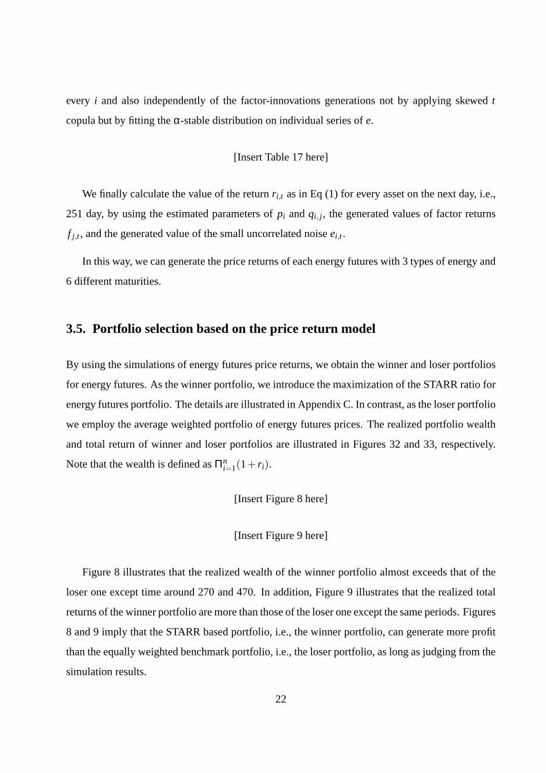
and total return of winner and loser portfolios are illustrated in Figures 32 and 33, respectively.

Note that the wealth is defined asΠni=1(1+ r i).



Figure 8 illustrates that the realized wealth of the winner portfolio almost exceeds that of the

loser one except time around 270 and 470. In addition, Figure 9 illustrates that the realized total

returns of the winner portfolio are more than those of the loser one except the same periods. Figures

8 and 9 imply that the STARR based portfolio, i.e., the winner portfolio, can generate more profit

than the equally weighted benchmark portfolio, i.e., the loser portfolio, as long as judging from the

simulation results.

22

Additionally, we also conduct another simulation. The results of two simulations are tabulated

in Table 18.


Note that the relative difference is defined by the ratio of the value of similation minus that of

benchmark over the value of benchmark.

Table 18 suggests that STARR ratios of the two are 3.085 and 3.033, respectively and they are

greater than that of benchmark of 1.508. Thus, the performance of the winner portfolios in energy

futures markets by using the STARR ratio is likely to be better than that of loser portfolio by using

the average return, as long as we employ the data in this paper.

Judging from Sharpe ratios as in Table 18, two simulations perform better than the benchmark

with the relative differences of 1.559 and 1.536, respectively. On the other hand, from STARR

ratios as in Table 18, two simulations perform better than the benchmark only with the differences

of 1.046 and 1.011, respectively. The differences come from the risk measures: the standard de-

viation for the Sharpe ratio on one hand and the ETL for the STARR ratio on the other hand. The

standard deviation captures the risk of the portfolio by assuming that the price returns follow nor-

mal distributions, while the ETL does it by assuming they do not necessarily follow normal ones.

Thus, the estimated standard deviations evaluate the portfolio risk less than the estimated ETLs.

Taking it into account that price returns of energy futures have the stable distribution innovations,

the STARR ratio may be more appropriate than the Sharpe ratio. It leads to the usefulness of

the STARR ratio so as to obtain higher performance portfolio than the average in energy markets

appropriately.

23

4. Conclusions and Directions for Future Research

This paper has examined the portfolio optimization of energy futures by using the STARR ratio

that can evaluate the risk and return relationship for skewed distributed returns. We have modeled

the price return for energy by using the ARMA(1,1)-GARCH(1,1)-PCA model with stable dis-

tributed innovations that reflects the characteristics of energy: mean reversion, heteroskedasticity,

seasonality, and spikes. Then, we have proposed the method for selecting the portfolio of energy

futures by maximizing the STARR ratio. The empirical studies by using energy futures prices of

WTI crude oil, heating oil, and natural gas traded on the NYMEX have compared the price return

models with stable distributed innovations to those with normal ones for energy futures. We have

show that the models with stable distributed innovations are more appropriate for energy futures

than those with normal ones. In addition, we have offered some arguments that the stable innova-

tions may come from price spikes in energy futures markets. Then, we generate the price returns by

using the proposed ARMA(1,1)-GARCH(1,1)-PCA model with stable ones and choose the port-

folio of energy futures. The results have illustrated that the selected portfolio performs better than

the average weighted portfolio. It implies that the STARR ratio may work well in selecting the

winner portfolio of energy futures.

This paper did not examine the performance of the long and short trading strategy in order to

focus on the method for selecting the winner portfolio in energy futures markets. We leave it to the

direction for our future research.

24

Appendix A. α-stable distribution

The log-returns of energy prices are well known for having high skewness and kurtosis. So it is difficult

to model such time series appropriately by using the normal distribution.α-stable distribution is often

introduced as a tool to model such high skewness and kurtosis. Unfortunately, it does not have distribution

function and density in closed form. Stable distributions are introduced by their characteristic function as

follows,

logF(t) =

−σα | t |α(

1− iβsgn(t) tan(πα2 )

)+ iµt, α 6= 0

−σ | t |(

1− iβ 2πsgn(t) log | t |

)+ iµt, α = 0,

(A1)

whereF(t) denotes the characteristic function of the stable law:

F(t) =Z

eitx 1σ

f

(x−µ

σ

)dx. (A2)

The parameterα describes the kurtosis of the distribution with0< α≤ 2. The smallerα, the heavier the tail

of the distribution. The parameterβ describes the skewness of the distribution,−1≤ β≤ 1. If β is positive

(negative), then the distribution is skewed to the right (left).µ andσ are the shift and scale parameters,

respectively. Ifα andβ equal 2 and 0, respectively, then theα-stable distribution reduces to the normal one.

Appendix B. The Algorithm

In the beginning, knowing the number of observationsN (N = 812) and return seriesRit , we determine

coefficientsa andb of the ARMA(1,1) model:Rt = a0 + a1Rt−1 + b1εt−1 + εt . Then, for that purpose we

have to solve the system of equations:

E[εi ] = 0,

E[εiεi−1] = 0,

E[εiεi−2] = 0

(B3)

25

If parametersa andb are found, we perform the next steps. We, then, restore empirical values of residuals

ε = (εt) from the ARMA(1,1) model:Rt = a0 +a1Rt−1 +b1εt−1 + εt based on found coefficientsa andb:

εt = Rt −a0−a1Rt−1−b1εt−1. (B4)

After we have found the residuals from ARMA(1,1), we finally apply the GARCH(1,1) model for them, ob-

tain innovations and check the hypotheses for normality and stability for the innovations of the GARCH(1,1)

model of the residuals from the ARMA(1,1) model. We determine parameters of stable distribution for the

sequence of innovations:a is the index of stability (a∈ (0,2]), b is the skewness parameter (b∈ [−1,1]), σ

is the scale parameter (σ ∈ R+), andµ is the shift parameter (µ∈ R).

Appendix C. Optimization Problem Solving for Energy Futures

maxzpl

STARRδ(r(p)) (C5)

STARRδ(r(p)) =R(p)

ETLδ(r(p)), (C6)

wherezpl is the weight of assetl in the portfolio ofn assets,r(p) is the total random return of the portfolio

consisting ofn assets:r(p) = ∑nl=1zplr l wherer l is the random daily return of assetl , R(p) = E(r(p)) =

∑nl=1zplRl is the total expected (daily) return of the portfolio ofn assets whereRl represents mean return

(expected value ofr l -vector of dimension equal to 250 working days), andn is set to 18 such thatzpl > 0

wherezpl is the weight of individual assetl in the portfolio ofn assets:

zp =n

∑l=1

zpl = 1, (C7)

n = 18. (C8)

26

References

Biglova, A., and S. Rachev, 2007, Portfolio Performance Attribution,Investment Management and Financial

Innovations4, 7–22.

Black, F., 1975, Fact and Fantasy in the Use of Options,Financial Analysts Journal31, 36–72.

Bollerslev, T., 1986, Generalized Autoregressive Conditional Heteroskedasticity,Journal of Econometrics

31, 307–327.

Erb, C., and C. Harvey, 2006, The strategic and tactical value of commodity futures,Financial Analysts

Journal62(2), 69–97.

Eydeland, A., and K. Wolyniec, 2003,Energy and Power Risk Management: New Developments in Model-

ing, Pricing, and Hedging. (John Wiley& Sons, Inc. Hoboken).

Gatev, E.G., W. N. Goetzmann, and K. G. Rouwenhorst, 2006, Pairs Trading: Performance of a Relative-

Value Arbitrage Rule,Review of Financial Studies19(3), 797–827.

Geman, H., 2005,Commodities and Commodity Derivatives. (John Wiley& Sons Ltd West Sussex).

Geman, H., and A. Roncoroni, 2006, Understanding the fine structure of electricity prices,Journal of Busi-

ness79, 1225–1261.

Hotelling, H., 1933, Analysis of a Complex of Statistical Variables with Principal Components,Journal of

Educational Psychology27, 417–441.

Huisman, R., and R. Mahieu, 2001, Regime Jumps in Power Prices,Energy& Power Risk Management,

September.

Jurek, J. W., and H. Yang, 2007, Dynamic Portfolio Selection in Arbitrage, Working paper, Harvard Univer-

sity.

Kanamura, T., 2006, A Supply and Demand Based Volatility Model for Energy Prices - The Relationship

between Supply Curve Shape and Volatility -, Working paper, Hitotsubashi University.

Miffre, J., and G. Rallis, 2007, Momentum strategies in commodity futures markets,Journal of Banking&

Finance31, 1863–1886.

27

Pilipovic, D., 1998,Energy Risk: Valuing and Managing Energy Derivatives. (McGraw-Hill New York).

Rachev, S., T. Jasic, A. Biglova, and F. Fabozzi, 2006, Risk and Return in Momentum Strategies: Prof-

itability from Portfolios based on Risk-Adjusted Stock Ranking Criteria, Working paper, University of

Karlsruhe.

Rachev, S., T. Jasic, S. Stoyanov, and F. Fabozzi, 2007, Momentum strategies based on reward - risk stock

selection criteria,Journal of Banking& Financepp. 2325–346.

Rachev, S., C. Menn, and F. Fabozzi, 2005,Fat-Tailed and Skewed Asset Return Distributions. (John Wiley

& Sons, Inc New Jersey).

Rachev, S., and S. Mittnik, 2000,Stable Paretian Models in Finance. (John Wiley& Sons, Inc. Chichester).

Rachev, S., S. Mittnik, F. Fabozzi, S. Focardi, and T. Jasic, 2007,Financial Econometrics. (John Wiley&

Sons, Inc New Jersey).

Rachev, S., S. Ortobelli, S. Stoyanov, F. Fabozzi, and A. Biglova, 2007, Desirable Properties of an Ideal Risk

Measure in Portfolio Theory,International Journal of Theoretical and Applied Financeforthcoming.

Figures& Tables

Figure 1. Scatter Plots between Index of Stabilityα and Skewness Parameterβ for DailyReturns of 18 Assets

28

Figure 2. Scatter Plots between Index of Stabilityα and Skewness Parameterβ for Innova-tions of GARCH(1,1) Fit of Daily Returns of 18 Assets

Figure 3. Simulation of ARMA(1,1) model of hn = a0+a1hn−1+b1εn−1+σεn, where a0 =−1,a1 = 0.5, b1 = 0.1, andσ = 0.1

29

Figure 4. Scatter Plots between Index of Stabilityα and Skewness Parameterβ for Innova-tions of ARMA(1,1)-GARCH (1,1) Fit of 18 Assets

Figure 5. Scatter Plots between Index of Stabilityα and Skewness Parameterβ for 7 Factors’Series

30

Figure 6. Scatter Plots between Index of Stabilityα and Skewness Parameterβ for Innova-tions of GARCH(1,1) Fit of 7 Factors’ Series

Figure 7. Scatter Plots between Index of Stabilityα and Skewness Parameterβ for Innova-tions of ARMA(1,1)-GARCH (1,1) Fit of 7 Factors’ Series

31

Figure 8. Realized Wealth of Winner and Loser Portfolios

Figure 9. Realized Total Return of Winner and Loser Portfolios

32

Confidence level 95% 99% 99.9% 99.95% 99.99%% of energy futures prices for which the 73.98 74.00 74.04 74.40 74.24normal distribution hypothesis is rejected% of energy futures prices for which the 7.10 7.14 7.34 7.13 6.62stable distribution hypothesis is rejected

Table 1. Normality and Stable Distribution Hypotheses for i.i.d. Model

α β KSdistances (normal) KSdistances (stable)Mean 1.8754 -0.5396 0.7398 0.0710Median 1.8923 -0.5368 0.7407 0.06771 quartile (25%) 1.8653 -0.7606 0.7241 0.04313 quartile (75%) 1.9021 -0.4082 0.7524 0.0997

Table 2. Summary of Statistics for Sample of 18 Assets on i.i.d. Model


Table 3. Normality and Stable Distribution Hypotheses for GARCH(1,1) model

33


Table 4. Summary of Statistics for Sample of 18 Assets on GARCH(1,1) Model


Table 5. Normality and Stable Distribution Hypotheses for ARMA(1,1)-GARCH(1,1) Model


Table 6. Summary of Statistics for Sample of 18 Assets on ARMA(1,1)-GARCH(1,1) Model

34

Principal component % of variance explained % of total variance explained1 66.8151 66.81512 23.9985 90.81363 3.5411 94.35484 1.8570 96.21185 1.3153 97.52726 0.9210 98.44827 0.5769 99.02518 0.3256 99.35089 0.2547 99.6056

10 0.1323 99.738011 0.1084 99.846512 0.0698 99.916413 0.0339 99.950314 0.0271 99.977415 0.0117 99.989216 0.0067 99.996017 0.0030 99.999018 0.0009 100

Table 7. % of Total Variance by Growing # of Components on Covariance Matrix


Table 8. Normality and Stable Distribution Hypotheses for i.i.d. PCA Model

α β KSdistances (normal) KSdistances (stable)Mean 1.5749 -0.1786 0.7507 0.1988Median 1.5245 0.0130 0.7573 0.14281 quartile (25%) 1.3897 -0.4025 0.7361 0.10923 quartile (75%) 1.8660 0.0713 0.7613 0.3303

Table 9. Summary of Statistics for Sample of 18 Assets on i.i.d. PCA Model

35


Table 10. Normality and Stable Distribution Hypotheses for GARCH(1,1)-PCA Model


Table 11. Summary of Statistics for Sample of 18 Assets on GARCH(1,1)-PCA Model

r j p qj,1 q j,2 q j,3 q j,4 q j,5 q j,6 q j,7

j = 1 0.007 0.190 0.085 0.170 0.126 0.154 0.026 -0.554j = 2 0.007 0.173 0.078 0.143 0.078 0.077 0.014 -0.094j = 3 0.006 0.157 0.072 0.135 0.071 0.033 0.001 0.032j = 4 0.006 0.144 0.066 0.130 0.065 0.009 0.000 0.103j = 5 0.006 0.134 0.062 0.124 0.061 -0.007 -0.003 0.154j = 6 0.005 0.126 0.058 0.119 0.055 -0.020 -0.005 0.188j = 7 0.020 0.549 0.103 -0.925 -0.197 1.395 0.408 0.528j = 8 0.022 0.515 0.142 -0.658 -0.132 0.408 0.119 -0.091j = 9 0.023 0.464 0.156 -0.502 -0.192 -0.059 -0.016 -0.183j = 10 0.024 0.426 0.160 -0.355 -0.232 -0.383 -0.094 -0.147j = 11 0.023 0.397 0.156 -0.251 -0.255 -0.535 -0.121 -0.069j = 12 0.023 0.373 0.144 -0.172 -0.252 -0.626 -0.134 0.003j = 13 0.003 0.030 -0.081 -0.067 0.144 0.003 -0.118 0.018j = 14 0.003 0.028 -0.073 -0.020 0.061 -0.035 0.026 -0.021j = 15 0.003 0.025 -0.065 0.000 0.017 -0.029 0.110 0.004j = 16 0.003 0.021 -0.051 0.017 -0.029 0.001 0.028 0.006j = 17 0.004 0.018 -0.044 0.021 -0.041 0.015 -0.028 -0.001j = 18 0.004 0.017 -0.041 0.021 -0.038 0.016 -0.040 -0.004

Table 12. ARMA(1,1)-GARCH(1,1) Model for Principal Components

36

f j a j,0 a j,1 b j,1 α0 α1 β1

j = 1 0.0042 0.5373 -0.6056 0.073 0.9059 0.0202j = 2 -0.0073 0.7114 -0.7787 0.0371 0.8619 0.1047j = 3 0.0070 0.3378 -0.3000 0.0513 0.9078 0.0421j = 4 0.0468 -0.4911 0.3571 0.0356 0.7329 0.2425j = 5 -0.0463 0.5192 -0.5566 0.4708 0.1682 0.5576j = 6 0.1039 -0.7754 0.2478 0.1421 0 0.9999j = 7 -0.0128 -0.2500 0.2048 0.5862 0 0.5913

Table 13. ARMA(1,1)-GARCH(1,1) Model for Principal Components (Cont’d)


Table 14. Normality and Stable Distribution Hypotheses for ARMA(1,1)-GARCH(1,1)-PCA Model


Table 15. Summary of Statistics for Sample of 18 Assets on ARMA(1,1)-GARCH(1,1)-PCA Model

f1 f2 f3 f4 f5 f6 f7γi -0.0542 -0.0671 -0.0116 0.0335 0.0236 -0.0157 -0.1251µi 0.1108 0.1709 0.0245 -0.0785 0.0505 -0.0440 0.2471ν 5

Table 16. Estimates of Skewedt Copula Parameters

37

ei a j,0 a j,1 b j,1 α0 α1 β1

i = 1 7.93E-06 0.113 -0.149 2.00E-07 0.871 0.062i = 2 -1.23E-05 -0.249 0.131 2.78E-07 0.892 0.036i = 3 -3.84E-06 0.556 -0.490 1.76E-07 0.835 0.066i = 4 -3.37E-06 -0.528 0.623 4.15E-08 0.840 0.061i = 5 4.75E-05 -0.696 0.678 4.40E-07 0.000 0.318i = 6 5.44E-05 -0.659 0.609 2.00E-07 0.834 0.071i = 7 3.23E-05 0.529 -0.530 4.03E-06 0.000 1.000i = 8 1.60E-04 -0.874 0.821 3.86E-06 0.019 0.935i = 9 4.35E-05 -0.917 0.890 8.19E-06 0.099 0.000i = 10 2.65E-05 -0.941 0.900 2.00E-07 0.954 0.000i = 11 -8.66E-06 -0.868 0.837 2.48E-06 0.233 0.000i = 12 2.77E-06 0.251 -0.317 8.70E-06 0.356 0.000i = 13 -4.71E-04 -0.992 1.000 5.04E-07 0.466 0.534i = 14 2.17E-04 0.150 -0.466 1.17E-06 0.493 0.507i = 15 -1.24E-06 0.766 -0.943 6.36E-07 0.735 0.265i = 16 6.85E-04 -0.881 0.898 5.21E-06 0.000 1.000i = 17 -2.82E-07 0.749 -0.726 1.29E-06 0.602 0.000i = 18 4.63E-07 0.593 -0.514 4.36E-06 0.469 0.000

Table 17. ARMA(1,1)-GARCH(1,1) Stable Distributed Innovations

Simulation No. 1 Simulation No. 2 BenchmarkMeasures Values Relative Values Relative

(daily, % ) difference (daily, % ) differenceAverage mean return 0.107 0.191 0.106 0.179 0.090Estimated ETL (99% ) 3.471 -0.418 3.493 -0.414 5.961STARR (99% ) 3.085 1.046 3.033 1.011 1.508Estimated standard deviation 0.862 -0.535 0.861 -0.535 1.852Sharpe Ratio 12.424 1.559 12.312 1.536 4.855

Table 18. Results of Simulations

38

modeling, risk assessment and portfolio optimization of energy futures

Documents