modeling relationship between geometric design … dwikat.pdfmohammed ghassan dwikat supervised dr....

An-Najah National University

Faculty of Graduate Studies

Modeling Relationship between Geometric Design

Consistency and Road Safety for Two-Lane Rural Highways

in the West Bank

By

Mohammed Ghassan Dwikat

Supervised

Dr. Khaled Al-Sahili

This Thesis is Submitted in Partial Fulfillment of the Requirements for

the Degree of Master of Roads and Transport Engineering, Faculty of

Graduate Studies, An-Najah National University, Nablus- Palestine.

2014

iii

DEDICATION

This thesis is dedicated with great love to my Angels; my dear parents who

have always supported me. I also dedicate it to the light of my life; my

brothers and sisters. Finally, I will not forget my great friends for always

being there for me.

iv

ACKNOWLEDGMENT

I am thankful to the almighty God for granting me good health, strength

and peace throughout the research period.

It is with great pleasure that I hereby express my appreciation to everyone

who has contributed, in one way or another, to the completion of this thesis

work. Without your assistance, this work would have proved

insurmountable.

I am highly indebted to my supervisors, Dr. Khaled Al-Sahili - Director of

Construction and Transportation Research Unit- and Prof. Sameer Abu-

Eishes- Interior Examiner, for their constant guidance during the whole

project period. I am also grateful for Dr. Wael AlhajYaseen . I am deeply

thankful for all the assistance that was rendered to me by the Faculty of

Engineering, An Najah National University. I am especially thankful to

Eng. Jamil M. J. Hamadneh for all the help he accorded me during writing

this thesis.

v

:

Modeling Relationship between Geometric Design Consistency and

Road Safety for Two-Lane Rural Highways in the West Bank

,

.

Declaration

The work provided in this thesis, unless otherwise referenced, is the

Researcher’s own work, and has not been submitted elsewhere for any

other degree or qualification.

Student's Name: :الطالب اسم

Signature: :التوقيع

Date: التاريخ :

vi

Table of Contents

No. Contents page

Dedication Acknowledgement Declaration List of Tables List of Figures List of Abbreviations Abstract CHAPTER ONE INTRODOCTION

1.1 Background 1.2 Evolution of the Concept of Design Consistency 1.3 Problem Statement 1.4 Study Area 1.5 Objectives And Scope 1.6 Thesis Structure

CHAPTER TWO LITERATURE REVIEW 2.1 Design Consistency Measures

2.1.1 Operating Speed 2.1.2 Vehicle Stability 2.1.3 Alignment Indices 2.1.4 Driver Workload 2.2 Relationships Of Consistency Measures To Safety 2.3 Previously Developed Crash Prediction Models 2.4 Summary

CHAPTER THREE RESEARCH METHODOLOGY 3.1 Literature Review 3.2 Data Collection 3.3 Modeling Methodology

3.3.1 Selection of Analysis Sites

vii

3.3.2 Horizontal Alignment 3.3.3 Statistical Technology 3.3.4 Estimating Consistency Measures 3.4 Modeling Validation 3.5 Modeling Apllication 3.6 Conclusions and Recommendations

CHAPTER FOUR DATA COLLECTION 4.1 Overview of Data Collected 4.2 Horizontal Alignment 4.3 Traffic Volume 4.4 Crashes Data 4.5 Design Speed 4.6 Operating Speed

CHAPTER FIVE MODEL DEVELOPMENT 5.1 Crash Prediction Models 5.2 Modeling Techniques

5.2.1 Selection of Regression Technique 5.2.2 Model Structure and Development 5.2.3 Goodness of Fit 5.3 Selected Consistency Measures

CHAPTER SIX MODELING RESULTS 6.1 Variable Selection 6.2 Regression Technique and Exposure Variable Selection 6.3 Multiple Regression Analysis

6.3.1 Select the ‘Core’ Models 6.3.2 Develop the ‘Full’ Models

CHAPTER SEVEN MODELING VALIDATION 7.1 Validation of Crash Prediction Models

7.1.1 The External Validation1 CHAPTER EIGHT MODELING APPLICATION

8.1 Model Variables Computation

viii

8.2 Evaluating the Safety Performance of Two-Lane Rural

Highways

8.3 Comparing the Results of Two Different Types of Crash

Prediction Models in Evaluating Road Safety

8.3.1 Qualitative Analysis 8.4 A Systematic Approach to Identify Geometric Design

Inconsistencies

8.4.1 Establishing the Threshold Value of the Safety-Consistency

Factor

8.4.2 Quantitative Analysis 8.4.3 Ability to Identify Geometrically Inconsistent Sections 8.4.4 Proposed Alignments

CHAPTER NINE CONCLUSIONS AND

RECOMMENDATIONS

9.1 Conclusions 9.2 Recommendations

References

ix

List of Tables

No. Table Page

1 Table 1.1. Road Crash At Rural-Highways in the West

Bank (ICBS, 2012)

3

2 Table 2.1. Previously Developed Speed Prediction Models 16

3 Table 2.2. Operating Speed Prediction Equations for

Passenger Vehicles on Two-Lane Highways (Fitzpatrick et

al., 2000b)

19

4 Table 2.3. Speed Reduction Models on Horizontal Curve

(Al-Masaeid et al., 1995)

22

5 Table 2.4. Operating Speed Prediction Models on

Tangents (Polus et al., 2000)

25

6 Table 2.5. Deceleration and Acceleration Rates at

Different Curve Radius (Fitzpatrick et al., 2000c)

26

7 Table 4.1. Summary of Selected Highway Segments 58

8 Table 4.2. Summary of Statistics for Main Variables Used

in Highway 60

60

9 Table 4.3. Summary Statistics for Main Variables Used in

Highway 55

60


in Highway 505

62


in Highway 90

65

12 Table 4.6. Population and Growth Rate in West Bank

(PCBS)

66

13 Table 4.7. Average Daily Traffic for the Studied Roadway

Sections

67

14 Table 4.8. Number of Crashes on Highway Segments 68

15 Table 4.9. Legal Speed Limit and Design Speed for

Selected Highways

69

16 Table 4.10. Summary of Statistics for Operating Speed

Used in the Studied Highway Sections

70

17 Table 5.1. Summary of Statistics of the Design consistency 84

x

Measures as Applied to the Alignments Under Study

18 Table 6.1 Models Developed Depending on Tangent Data

Only (111 Tangents)

88

19 Table 6.2 Models Developed Depending on Horizontal

Curves Data Only (136 Horizontal Curves)

90

20 Table 6.3 Models Developed Depending on Horizontal

Curves and Tangents Data Combined (136 Horizontal

Curves and 111 Tangents)

92

21 Table 6.4 The ‘Core’ Models 95

22 Table 6.5. Pearson's Correlation Coefficients Matrix for

Potential Variables Measure

100

23 Table 6.6 Model for Predicting Safety Performance of

Tangent Sections Only

100


Horizontal Curves Only Depending on V85 - VD and ∆V85

101


Horizontal Curves Only Depending on V85 - VD and CRR

102


Horizontal Curves Only Depending on V85 - VD and VDLU

102

27 Table 6.10. Summary for Variables Used in Developing

Model "V"

104


Tangent and Horizontal Curves Combined

105

29 Table 7.1 Validation Statistics for Models I to V Total

Section-Related Accidents

116

30 Table 8.1. Horizontal Alignment Data of Two Fictitious

Alignments (Hassan et al, 2001)

121

31 Table 8.2. Model (V) Crash Prediction Frequency per-

Year

123

xi

List of Figures

No. Figure Page

1 Figure 1.1. Location of the Study Highway Segments in the

West Bank

8

2 Figure 2.1. Distribution of Observation Points on a Typical 3D

Combination (Gibreel et al., 2001)

20

3 Figure 4.1. Location of the Study Highway Segments in the

West Bank

57

4 Figure 4.2: Ortho-Drawing for Highway 60 with Accident

Locations

59

5 Figure 4.3. Ortho-Drawing for Highway 55 with Accident

Locations

61


Locations

63


Locations

64

8 Figure 4.6. Real Time Speed for Individual Car Driver 71

9 Figure 7.1. Location of the Highway Segments for Validation

in the West Bank

107

10 Figure 8.1. Plans of the Two Fictitious Alignments (Hassan et

al, 2001)

122

11 Figure 8.2. Predicted Crash Frequency of the Two Fictitious

Alignments Based on Model (V)

126

12 Figure 8.3. Predicted Crash Frequency of the Two Fictitious

Alignments Based on the Algorithm in HSM

129

13 Figure 8.4. Cumulative Distribution of the Safety-Consistency

Factors of Horizontal Curves of an Existing Alignment

132

14 Figure 8.5. Safety-Consistency Factors Based on Model (V) of

the Two Fictitious Alignments

133

15 Figure 8.6. Safety-Consistency Factors Based on HSM Module

of the Two Fictitious Alignments

13

xii

List of Abbreviations

PCBS = Palestinian Central Bureau of Statistics

ICBS = Israeli Central Bureau of Statistics

VD = design speed of the highway

V85 = 85th percentile operating speed

∆V85 = absolute difference of the 85th

percentile speeds between successive

design elements

VD = design speed

R = radius of the curve

CCR = curvature change rate

AADT = average annual daily traffic

AADT = average daily traffic

VD = design speed

85MSR = the 85th

percentile maximum speed reduction

DC = degree of curvature

DF = deflection angle

∆fR = difference between side friction supplied and demanded

xiii

fS = side friction supplied

fD = side friction demanded

fTP = maximum permissible tangential friction factor

fRPerm. = maximum permissible side friction factor

fr = coefficient of side friction

AVG R = Average radius of curvature

= Maximum radius of curvature to minimum radius of curvature

AVG T = Average tangent length

CCR = Curvature change rate

CRR = Ratio of individual curve radius to average radius

VDLF = visual demand of familiar drivers

VDLU = visual demand of unfamiliar drivers

Nbr = predicted number of total accidents per year on a particular roadway

segment.

EXPO = exposure in million vehicle-miles of travel per year

Cr./5yrs = predicted crash frequency per 5 years

xiv

AASHTO = American Association of State Highways and Transportation

Officials

GLM = generalized linear regression method

CPM = Crash prediction model

kD = dispersion parameter depending on scaled deviance,

kP = dispersion parameter depending on Pearson Ӽ 2

SD = scaled deviance value of model

Pearson Ӽ2 = Pearson chi-squared value of model

EXP = Exponential function, e = 2.718282

kmax = maximum dispersion parameter of the model

MPB = mean prediction bias

MAD = mean absolute deviation

MSPE = Mean squared prediction error

MSE = Mean squared error

GOF = goodness-of-fit

HSM = highway safety manual

CMFH = crash modification factor for horizontal curves

xv

Nrs = predicted number of total crashes per year on a section

SCF = safety consistency factor

xvi

Modeling Relationship between Geometric Design Consistency and

Road Safety for Two-Lane Rural Highways in the West Bank

By

Mohammed Ghassan Dwikat

Supervised

Dr. Khaled Al-Sahili

Abstract

The objectives of this study are to investigate and quantify the relationship

between design consistency and road safety for two-lane highways in the

West Bank. This study produced speed prediction method using real time

traffic speed data obtained from Google Earth maps, which were used to

estimate the 85th percentile speed along an alignment that includes both

horizontal curve sections and tangent sections. A comprehensive crash and

geometric design database of two-lane rural highways has been used to

investigate the effect of several design consistency measures on road

safety.

Previous studies showed that the most promising consistency measures

identified in previous research fall into four main categories, namely:

operating speed, vehicle stability, alignment indices, and driver workload.

Five crash prediction models, which relate design consistency to road

safety, have been examined. The generalized linear regression approach has

been used for model development. All models adopted in this study showed

acceptable levels of goodness of fit and over-dispersion. The developed

models verified that the main design consistency measures have an

important impact on safety. The consistency measures used in model

development are: variation between the design speed and the operating

xvii

speed, absolute difference of the 85th percentile speeds between successive

design elements, difference between side friction supplied and demanded,

average radius of curvature, average tangent length, maximum radius of

curvature to minimum radius of curvature, curvature change rate, ratio of

individual curve radius to average radius of the section, and visual demand

of familiar drivers of the section.

Validation step was performed; the goal was not only to compare the

accuracy of different models developed, but also to evaluate the overall

accuracy of Crash Prediction Models for use on rural two-lane highways in

the West Bank. Validation requirement was to demonstrate that a model is

appropriate, meaningful, and useful for the purpose for which it is intended.

The models can be used as a quantitative tool to evaluate the impact of

design consistency on road safety. An application is presented where the

effectiveness of crash prediction models, which incorporate design

consistency measures, is compared with those, which rely on geometric

design characteristics. The study concluded that models, which explicitly

consider design consistency, can identify the inconsistencies more

effectively and reflect the resulting impacts on safety more accurately than

those which do not. Finally, a systematic approach to identify

geometrically inconsistent locations using the safety consistency factor has

been proposed.

1

Chapter One

Introduction

This chapter gives the necessary background information to understand

why a quantitative relationship between design consistency and road safety

needs to be investigated. In addition, the sources of design inconsistency in

current geometric design practice are presented. Furthermore, this chapter

gives a brief summary about evolution of the concept of design

consistency. The problem statement and how study area will be chosen is

presented. Finally, it presents the objectives and the structure of this thesis.

1.1 Background

The goal of transportation is generally stated as the safe and efficient

movement of people and goods. To achieve this goal, designers use many

tools and techniques. One technique used to improve safety on roadways is

to examine the consistency of the design. Design consistency refers to a

highway geometry’s conformance with driver expectancy. Generally,

drivers make fewer errors at geometric features that conform with their

expectations than at features that violate their a priori and/or ad hoc

expectancies (Alexander and Lunenfeld, 1986).

Driver expectancy is shaped by experience, which is largely dependent on

the number of times a driver has driven on a particular road, the similarity

of the road to others in the driver's experience, and the accuracy of recent

predictions that have been made about the road (Fitzpatrick et al., 2000a).

2

Thus, a design inconsistency in a roadway segment implies a geometric

feature or features that violate driver expectancy, such as an abrupt change

in roadway geometry. Surprising drivers by violating their expectancies

increases the chance of delayed response times, speed errors, and unsafe

driving maneuvers that may lead to higher crash risk. To avoid these

problems, designers should ensure that the roadway design complies with

driver expectations through the evaluation of design consistency, and the

redesign of inconsistent locations.

Traffic crashes represent obsession for all members of society, and has

become one of the most important problems that drain material resources,

human potentials and targeting communities in the most important

elements of life which is the human element. In addition, the incurred

social, psychological problems and material losses are huge, which have

become imperative work to find solutions and suggestions and put them

into practice to reduce these crashes or at least handling the causes and

mitigate the negative effects.

Palestine experiences significant number of road crash at rural-highways in

the West-Bank, some of which result in fatal, serious or slightly injuries

which are presented in Table (1.1).

3

Table 1.1. Road Crash At Rural-Highways in the West-Bank

(ICBS, 2012).

Year Total

Crash

Fatal

Crash

Serious

Crash

Minor

Crash Casualties Dead

Serious

injured

Slight

injured

2003 525 27 100 398 1291 35 147 1109

2004 485 32 83 370 1205 37 121 1047

2005 516 21 99 396 1437 28 164 1245

2006 501 29 99 373 1440 37 148 1255

2007 548 24 93 431 1417 32 134 1251

2008 577 18 111 448 1473 19 153 1301

2009 552 21 92 439 1408 29 136 1243

2010 594 18 92 484 1450 22 114 1314

2011 542 29 72 441 1319 40 100 1179

2012 586 20 86 480 1395 29 120 1246

Crash data on the study road segments were acquired from the Israeli

Central Bureau of Statistics (ICBS), which includes the number of crashes

for 10 consecutive years; 2003 through 2012. The reliance on the ICBS for

crash data was because most rural highways are located in area (C), which

is out of control the Palestinian National Authority. Therefore, very limited

data is available for those highways from Palestinian sources.

The importance of design consistency and its significant contribution to

road safety can be justified with an understanding of the driver-vehicle-

roadway interaction. Roadway geometry, traffic conditions, and roadside

environment are the primary inputs to the driving task and determine the

4

workload requirement on the driver. How quickly and how well these

inputs are handled depend on driver expectancy and other human factors.

Once these inputs are processed, they are translated into vehicle

operations.

Lamm et al. (1986) have reported that half of all crashes on two-lane rural

highways may be indirectly attributed to inadequate speed adaptation,

indicating that design consistency is related to safety. Yet, despite the

importance of geometric design consistency to road safety, it is not always

ensured in current design practice.

An “inconsistency in design” can be described as a geometric feature or

combination of features with unusual or extreme characteristics that

drivers may drive in an unsafe manner. This situation could lead to speed

errors, inappropriate driving maneuvers, and/or an undesirable level of

accidents (Gibreel, 1999 and Fitzpatrick et al, 2000a).

1.2 Evolution of the Concept of Design Consistency

The development of consistent design practices has been a goal since at

least the 1930s. Barnett (1936) developed the concept of design speed to

ensure consistency. The design speed concept has undergone several

modifications in recent years, but the underlying theory still exists;

roadway alignments should meet or exceed the criteria for a given design

speed. Although sound in theory, problems have developed with the design

speed concept in its current form.

5

Design requires alignment features to be developed individually.

Difficulties arise when designers do not consider the roadway as a single

element consisting of several parts, the driver, geometry, and environment.

Conceptually, a breakdown in any one of these parts results in a location

with a high potential for crashes. Designers cannot control two of these

elements, but may account for them through the geometry. A relationship

exists between traffic safety and geometric design consistency, and

alignment consistency represents a key issue in modern highway geometric

design (Lamm et al., 1999). A consistent alignment will allow most drivers

to operate safely at their desired speed along the entire alignment.

Existing design speed-based alignment policies in AASHTO (2011)

encourage the selection of design speeds that are “. . . consistent with the

speeds that drivers are likely to expect on a given highway facility” and

that “fit the travel desires and habits of nearly all drivers expected to use a

particular facility”. Researchers have focused on developing methods to

account for problems associated with design consistency. The principal

focus in most of these studies has been on developing measures or

techniques to identify locations that may pose expectancy problems for the

driver. The measures most commonly used in previous studies have

focused on driver expectancy, speed prediction, or driver workload. These

terms will be explained in details in later chapter of this thesis.

6

1.3 Problem Statement

Considering sources of design inconsistency in current geometric design

practice, the impact of inconsistencies of existing alignments on road

safety must be investigated.

The length of main and regional highways in the West Bank is 1757 km

(PCBS, 2010); almost all rural roads are two-lane highways. Rural

highways have the greatest proportion of crashes on the West Bank

highway system. These crashes are frequently attributed to either driver

error or inadequate design. Unfortunately, the definition of inadequate

design is not clear because a combination of factors can all be detrimental

to a roadway design that meets or exceeds design standards. Although

designers attempt to address these issues, there has been concern that

designers are not doing enough to address them. Most research focuses on

geometric design elements and their relationships to safety. However, the

inconsistency in design affects driver's expectation; this may lead to human

error and potential road crash.

In the Palestinian area, there are no studies that address the effect of design

inconsistency, a factor that is related to road geometry and affects human

behavior, on road safety. Therefore, this thesis investigates the relationship

between design inconsistency and road safety on two-lane rural highways

in the West Bank, which form the vast majority of rural highways.

7

1.4 Study Area

Four two-lane rural highway segments located in the West Bank were

chosen in this study. The selection of these highways was mainly based on

limitations in data availability. However, it was ensured that the selected

highways encompass a variety of highway classifications, locations,

terrain, design speed, traffic volume, and crash history in West Bank.

Figure (1.1) presents locations of the study highway segments in the West

Bank. Most of these highways and their segments were used for modeling

the relationship between design consistency and road safety and part of

them was set aside for validation purposes once the models are developed,

as will be explained later.

1.5 Objectives and Scope

This research is conducted with the following objectives:

1. To investigate and to quantify the relationship between design

consistency and road safety in terms of expected crash frequency.

2. To determine whether models which explicitly consider design

consistency are more effective in identifying inconsistencies on an

alignment and reflecting the impact on crash frequency than existing

models which rely on geometric design characteristics to predict crash

frequency.

8

3. To develop a systematic approach to identify geometric design

inconsistencies using crash prediction models.

Figure 1.1. Location of the Study Highway Segments in the West Bank

9

1.6 Thesis Structure

This thesis consists of nine chapters. Chapter one presents the necessary

background information to understand why a quantitative relationship

between design consistency and road safety needs to be investigated

besides the sources of design inconsistency in current geometric design

practice. Chapter two provides an extensive literature review on design

consistency and its relationship to safety. Chapter three describes the

methodology adopted for analysis. Chapter four describes the data used to

develop quantitative relationships between design consistency and safety.

Chapter five explain the methodology to develop the models relating

design consistency to safety. Chapter six shows the modeling results along

with a detailed discussion. Chapter seven evaluate the accuracy of the

West-Bank crash prediction models (CPM) developed. Chapter eight

includes three applications of the developed models. Finally, Chapter nine

brings forward the conclusions and gives some recommendations for

future research. The references are included in the end of this thesis.

10

Chapter Two

Literature Review

This chapter provides a review for potential measures of geometric design

consistency and its relationship to road safety. It also provides a review of

some models used for predicting consistency measures and corresponding

evaluation criteria.

2.1 Design Consistency Measures

Researches in design consistency focused on quantifying measures of

design consistency and developing models and evaluation criteria to

identifying them. The measures can be classified into four main classes:

operating speed, vehicle stability, alignment indices, and driver workload.

2.1.1 Operating Speed

The 85th percentile of free-flow speed distribution is commonly used to

represent “operating speed” for design consistency evaluations. Operating

speed is defined as the speed selected by highway users when not

restricted by other users, and is normally represented by the 85th percentile

speed. In terms of geometric design consistency, operating speed (V85) is

widely considered to be the most notable and straightforward geometric

design consistency measure (Poe and Mason, 2000). The change in speed

of vehicles is a visible indicator of inconsistency in geometric design.

Several interpretations of operating speed as a geometric design

consistency measure have been made in the literature. The operating speed

11

can be used in consistency evaluation by examining the variation between

the design speed (VD) and (V85) on a particular section of highway or

examining the differences between (V85) on consecutive highway elements

(∆V85).

Speed errors may be related to inconsistencies in horizontal alignment that

cause the driver to be surprised by sudden changes in the road's

characteristic, to exceed the critical speed of a curve and to lose control of

the vehicle. These inconsistencies can and should be controlled by the

engineer, when a roadway section is designed or improved (Lamm et al.,

1999).

Predicted operating speeds are compared to each other or to the designated

design speed to evaluate design consistency and crash risk (Cafiso and

Cerni, 2011). It is therefore of primary interest to develop methodologies

suitable for estimating the speed behavior of drivers. The traditional

approach to evaluating design consistency is based on calculating the

operating speed of the drivers separately on the curved and the tangent

sections. Speed differential between curve and tangent is used to evaluate

the consistency in the transition between two successive geometric

elements (Lamm et al., 2007). Based on these assumptions, numerous

models for estimating the operating speed exist in the literature.

12

2.1.1.1 Design Speed Based Measures

Since the 1930s, the design-speed concept has been the principal

quantitative mechanism for ensuring consistency of safe operating speeds

along rural highway alignments. The concept arose from safety concerns

about differentials between the speeds at which drivers could safely

operate their vehicles on tangents and the lower speeds at which they could

safely operate on horizontal curves. The solution implemented by the

design speed concept was that all alignment features should be designed to

accommodate the desired speeds of most drivers using the roadway or, in

other words, that an appropriate design speed should be uniformly applied

to all alignment elements of the roadway (Fitzpatrick et al., 2000a).

The design speed consistency measure is based on the deviation of design

speed from operating speed. The greater the difference between operating

speed and design speed, the worse the consistency evaluation. This

measure is used to check if actual driver speed meets design speed or not.

2.1.1.2 Operating Speed Based Measures

Speed differential between curve and tangent is used to evaluate the

consistency in the transition between two successive geometric elements,

which is usually expressed as the difference in the 85th

percentile operating

speeds (∆V85) between successive design elements.

Hirsh (1987) argued that calculating the speed differential by the simple

subtraction of the two related 85th percentile speed values on tangent and

13

curve would not give reasonable results due to the fact that the speed

distributions at the two locations are different. In addition, each driver

responds differently to the horizontal curve based on his/her desirable

tangent speed and the actual side friction factor. Thus, the 85th percentile

driver at one section is not necessarily the same 85th percentile driver at the

second section. As an alternative to subtraction of operating speeds, Hirsh

(1987) suggested that the full distribution of speed changes as incurred by

each driver should be examined to calculate the speed differential value.

Another approach has been proposed to examine by McFadden and

Elefteriadou (1999) for analyzing design consistency; the 85th percentile

maximum reduction in speed (85MSR). This parameter is calculated using

each drivers speed profile from approach tangent to horizontal curve and

determining the maximum speed reduction each driver experiences. The

85MSR was compared to the difference in 85th percentile speeds and was

found that the 85MSR is significantly larger than the difference in 85th

percentile speeds. The data showed that on average, 85MSR is two times

larger than the difference in 85th

percentile speeds.

2.1.1.3 Geometric Design Consistency Evaluation Criteria Based on

Design Speed and Operating Speed

Leisch and Leisch (1977) concluded that design speed reductions should

be avoided, but if they are necessary, they should not exceed 15 km/h.

Lamm et al. (1999) considered individual design elements (curves or

tangents) along the observed roadway section, the absolute difference

14

between the 85th

percentile speed and the selected design speed should

correspond to certain ranges:

1. Good design: V85 - VD ≤ 10 km/h (consistency),

2. Fair design: 10 km/h < V85 - VD ≤ 20 km/h (minor inconsistency; traffic

warning devices required),

3. Poor design: V85 - VD >20 km/h (strong inconsistency; redesign

recommended).

Note: V85 = 85th percentile operating speed (km/h); VD = design speed of

the roadway.


Operating Speed

Lamm et al. (1998) quantified design consistency based on operating speed

depending on the absolute difference of the 85th

percentile speeds between

successive design elements (tangent to curve or curve to curve) should fall

into certain ranges:

1. Good design: ∆V85 ≤ 10 km/h (consistency),

2. Fair design: 10 km/h < ∆V85 ≤ 20 km/h (minor inconsistency; traffic

warning devices required),

3. Poor design: ∆V85 > 20 km/h (strong inconsistency; redesign

recommended).

15

Note: ∆V85 = absolute difference of the 85th percentile speeds between

successive design elements (km/h).

A consistent and safe design when the difference between the operating

speeds as on two successive elements must be less than 15% of the speed

on the preceding quoted element (Babkov, 1975). Speed reduction from

tangent to the following curve design consistency evaluation criteria also

concluded by Kanellaidis et al. (1990) and Al-Masaeid et al. (1995) that

speed reduction from tangent to the following curve does not exceed 10

km/h (Good design).

2.1.1.5 Operating Speed Prediction Models on Curves

Numerous operating speed prediction models have been developed

worldwide. Table (2.1) reviewed some previously developed speed

prediction models.

Lamm and Choueiri (1987) found that the most significant parameter that

affects operating speed was the radius of horizontal curve. Another study

was performed by Kanellaidis et al. (1990) on driver’s speed behavior on

horizontal alignments. The authors found that the radius of horizontal

curve was the most significant parameter affecting operating speed using

regression analysis.

16

Table 2.1. A Sample of Previously Developed Speed Prediction Models

on Horizontal Curves.

Author Model R2

Lamm and Choueiri (1987) (Note: Several potential

variables and model forms

were tested as presented)

V85=88.72-0.084CCR [ LW=3.0 m ]

V85=89.55-(2862.69/R) [ LW=3.0 m ]

V85=92.69-0.080CCR [ LW=3.3 m ]

V85=93.83-(2955.40/R) [ LW=3.3 m ]

V85=95.77-0.076CCR [ LW=3.6 m ]

V85=96.15-(2803.70/R) [ LW=3.6 m]

V85=94.39-(3,188.57/R)=93.85-0.045CCR

V85=55.84-

(2,809.32/R)+0.634LW+0.053SW+ 0.0004

AADT

0.860

0.753

0.731

0.746

0.836

0.824

0.787

0.842

Kanellaidis et al. (1990) (Note: Several potential

variables and model forms


V85=109.09-(3837.55/R)

V85=32.20+0.839VD+(2226.9/R)-

(533.6/ R)

V85=129.88-(623.1/ )

0.647

0.925

0.777

Morrall and Talarico

(1994) V85=e

(4.561 - 0.00586 DC) 0.631

Islam and Seneviratne

(1994) (Note: Several model forms


V85=95.41-1.48DC-0.012DC2; (At PC)

V85=103.30-2.41DC-0.029DC2; (At MC)

V85=96.11-1.07DC; (At PT)

V85=103.66-1.95DC

0.990

0.980

0.980

0.800

Krammes et al. (1995) V85=102.45-1.57DC+0.0037LC-0.10DF 0.820

McFadden and

Elefteriadou (1997)

V85=41.62-1.29DC+ 0.0049LC-

0.12DF+0.95 VT

0.90

Note : V85 = 85th percentile speed (km/h); R = radius of the curve (m); CCR = curvature

change rate (degree/km); LW = lane width (m); SW = shoulder width (m); AADT =

average annual daily traffic (vehicles/day); VD = design speed (km/h); DC = degree of

curvature (degrees) expressed in degree per 30 m; PC = point of curvature; MC = middle

of curve; PT = point of tangent; LC = length of horizontal circular curve (m); DF =

deflection angle of horizontal curve (degrees); VT = approach tangent speed (km/h).

In another study, three operating speed prediction models were developed

by Islam and Seneviratne (1994) at different points along horizontal

curves. It was noticed that there were significant differences between the

operating speed values on the same horizontal curve at the point of curve

(PC), the middle of curve (MC), and point of tangent (PT). Therefore, they

recommended that design consistency should be evaluated based on the

difference between the operating speed at the point of tangent (PT) and the

17

design speed of the horizontal curve. These differences were found to

increase as the degree of curvature increased. Therefore, Gibreel et al.

(1999) suggested that speed consistency problems may tend to arise along

sharp horizontal curves. Morall and Talarico (1994) collected speed data

for nine horizontal curve sites on rural two-lane highways in Alberta,

Canada using a radar speedometer. Linear, multiplicative, exponential, and

reciprocal regression models were investigated and were found to provide

the best fit to the data. Krammes et al. (1995) and McFadden and

Elefteriadou (1997) developed new models taking into consideration new

parameters (length of horizontal circular curve, deflection angle of

horizontal curve and approach tangent speed) which reflect better model

fit.

Several different efforts were undertaken from Fitzpatrick et al. (2000b) to

predict operating speed for different conditions such as on horizontal

curves, vertical curves, and on a combination of horizontal and vertical

curves; on tangent sections; and prior to or after a horizontal curve. Speed

data were collected at over 200 two-lane rural highway sites for use in the

project. Regression equations were developed for passenger car speeds for

most combinations of horizontal and vertical alignment. Table (2.2) lists

the developed equations and/or the assumptions made for the different

alignment conditions for passenger cars.

Table (2.2) shows that, in most cases, V85 was predicted using the inverse

of the horizontal curve radius or the inverse of the rate of vertical

18

curvature. In cases where the sample size was too small to estimate a

model, the desired speed was assumed to be 100 km/h, based on the earlier

study by Krammes et al. (1995).

Although the models in Table (2.2) were developed with the consideration

of the presence of grade and/or vertical curves, the length of either

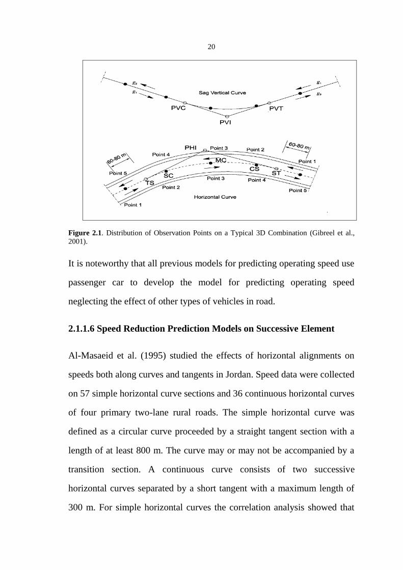
horizontal or vertical curve was not included. Gibreel et al. (2001)

developed a set of models, which considered the three-dimensional nature

of highways. The resulted coefficients of determination (R2) of the 3-D

models ranged from 0.79 to 0.98. Operating speed data were collected at

five points on each site to establish the effect of the 3-D alignment

combination on the trend of operating speed of the traveling vehicles (see

Figure 2.1).

Multiple linear regression technique was used to estimate the operating

speed models based on data collected on Highway 61 and Highway 102 in

Ontario, Canada. The results show that there is a significant difference

between the predicted operating speed using the 2-D and 3-D models.

19

Table 2.2. Operating Speed Prediction Equations for Passenger

Vehicles on Two-Lane Highways (Fitzpatrick et al., 2000b).

ACEQ# Alignment Condition Equation R2

1. Horizontal Curve on Grade : -

9% ≤ G < -4%

V85=102.10 - 3077.13/R 0.58

2. Horizontal Curve on Grade : -

4% ≤ G < 0%

V85=105.98 - 3709.90/R 0.76

3. Horizontal Curve on Grade :

0% ≤ G < +4%

V85=104.82 - 3574.51/R 0.76

4. Horizontal Curve on Grade :

+9% ≤ G < +4%

V85=96.61 - 2752.19/R 0.53

5. Horizontal Curve Combined

with Sag Vertical Curve

V85=105.32 - 3438.19/R 0.92


with Non-Limited Sight

Distance Crest Vertical Curve

(see note 3) N/A


with Limited Sight Distance

Crest Vertical Curve i.e., K ≤

43 m/%

V85=103.24 - 3576.51/R

(See note 4)

0.74

8. Sag Vertical Curve on

Horizontal Tangent

V85= assumed desired

speed

N/A

9.

Vertical Crest Curve with Non

Limited Sight Distance (i.e., K

> 43 m/%) on Horizontal

Tangent

V85= assumed desired

speed

N/A

10. Vertical Crest Curve with

Limited Sight Distance (i.e., K

≤ 43 m/%) on Horizontal

Tangent

V85=105.08 - 105.08/K

0.60

NOTES:

1. ACEQ# = Alignment Condition Equation Number;

2. Where: V85 = 85th percentile speed of passenger cars (km/h); K = rate of vertical

curvature; R = radius of curvature (m); G = grade (%);

3. Use lowest speed of the speeds predicted from equations 1 or 2 (for the

downgrade) and equations 3 or 4 (for the upgrade);

4. In addition, check the speeds predicted from equations 1 or 2 (for the downgrade)

and equations 3 or 4 (for the upgrade) and use the lowest speed.

20

Figure 2.1. Distribution of Observation Points on a Typical 3D Combination (Gibreel et al.,

2001).

It is noteworthy that all previous models for predicting operating speed use

passenger car to develop the model for predicting operating speed

neglecting the effect of other types of vehicles in road.

2.1.1.6 Speed Reduction Prediction Models on Successive Element

Al-Masaeid et al. (1995) studied the effects of horizontal alignments on

speeds both along curves and tangents in Jordan. Speed data were collected

on 57 simple horizontal curve sections and 36 continuous horizontal curves

of four primary two-lane rural roads. The simple horizontal curve was

defined as a circular curve proceeded by a straight tangent section with a

length of at least 800 m. The curve may or may not be accompanied by a

transition section. A continuous curve consists of two successive

horizontal curves separated by a short tangent with a maximum length of

300 m. For simple horizontal curves the correlation analysis showed that

21

speed reduction is highly correlated with the degree of horizontal curve,

length of vertical curve within horizontal curve, gradient, and pavement

conditions. The analysis revealed that lane and shoulder width,

superelevation, prevailing terrain, and posted speed had no effect on speed

reduction. The degree of the horizontal curve was the most important

variable for predicting the speed reduction. Models which have been

developed by Al-Masaeid et al. (1995) to predict speed reduction are

shown in Table (2.3).

Abdelwahab et al. (1998) developed a new model to predict speed

reduction taking degree of curvature and deflection angel as independent

variable, shown in Equation 2.1.

∆V85= 0.9433DC + 0.0847DF; R2 =

0.92 (2.1)

Where:

∆V85 = speed reduction between tangent and of curve (km/h);

DC = degree of curvature (degrees) expressed in degree per 30 m;

DF = deflection angle (degree).

The study size was 46 curves, 35 observations per curve, which were

located in Jordan. The authors argued that despite the statistical correlation

that may exist between degree of curvature and deflection angle, the

inclusion of these two basic variables in a speed reduction model is

expected to improve its performance.

22

Table 2.3. Speed Reduction Models on Horizontal Curve (Al-Masaeid

et al., 1995).

Models

Simple curves

1. ∆V85PC =3.64+1.78DC

2. ∆V85LT =2.0DC

3. ∆V85HT =4.32+1.44DC

4. ∆V85ALL =3.30+1.58DC

5. ∆V85ALL =1.84+1.39DC+4.39Pcon.+0.07G2

6. ∆V85ALL =1.45+1.55DC+4.0Pcon+0.00004LVC2

0.51

0.69

0.42

0.62

0.77

0.76

Compound Curves

7. ∆V85PC = (5708/R2)-(5689/R1)

8. ∆V85LT = (4957/R2)-(4888/R1)

9. ∆V85HT = (5463/R2)-(5463/R1)

10. ∆V85ALL = (5081/R2)-(5081/R1)

0.72

0.77

0.66

0.81 Note: ∆V85 = speed reduction between tangent and of curve (km/h); DC = degree of

curvature (degrees) expressed in degree per 30 m; Pcon. = pavement condition

(PSR 3, Pcon = 0, otherwise = Pcon=0, PSR: Present Serviceability Rating; G =

gradient (average slope between the points of speed measurements on the tangent

and the curve center, (%));

LVC = length of vertical curve within the horizontal curve (m); R1, R2 = radius of

preceding and succeeding curves respectively (m); PC = Passenger car; LT = Light

Truck; HT = Heavy Truck; ALL = all type of vehicles.

Another study was done by McFadden and Elefteriadou (1999) for the

purpose of using V85 profiles to evaluate design consistency on two-lane,

rural highways. Speed data were collected at 21 horizontal curves. The 85th

percentile maximum speed reduction (85MSR) was modeled as a function

of road geometry.

Studies of Al-Masaeid et al. (1995); Abdelwahab et al. (1998); and

McFadden and Elefteriadou (1999) focused on developing models for the

speed reduction from a tangent to a curve. However, only one of them,

McFadden and Elefteriadou (1999), considered the speed reduction

through tracking the speed of individual vehicles along the curve. The

23

other two just subtracted the 85th

percentile speed value at the middle of

the curve from that of the tangent.

2.1.1.7 Operating Speed Prediction on Tangents

Based on Lamm et al. (1999) independent tangents are those tangents long

enough to permit acceleration to and deceleration from the free-flow speed.

On the other hand, non-independent tangents are those tangents that are too

short to permit acceleration and have speeds similar to their preceding

curve. Tangents less than approximately 180 m in length were considered

to be non-independent (Lamm et al., 1999). Misaghi and Hassan (2005)

suggested that length of non-independent tangents is less than 200 m. For

operating speed on approach tangents, average values of the observed 85th

percentile speed were recommended as 103.0 km/h for independent

tangents and 95.8 km/h for non-independent tangents. On the other hand,

Lamm and Choueiri (1987) used a value of 94.7 km/hr and Krammes et al.

(1995) used a value of 97.9 km/hr for the 85th speed of the independent

tangents. Hassan et al. (2000) recommended the value 102.0 km/h for

independent tangent.

Several models were developed to predict the operating speed on

independent tangent based on data collected in Jordan (Al-Masaeid et al.,

1995). It is found that the operating speed is affected by the length of the

independent, the degree of successive horizontal curves, and the deflection

angles of the two curves.

24

The operating speed on independent tangents is more complex and

depends on a whole array of roadway character, making it difficult to

develop reasonably accurate prediction models. It is significantly

influenced by the preceding and succeeding horizontal curves (Joanne,

2002).

Polus et al. (2000) developed models for predicting operating speeds on

162 non-independent and independent tangents. In addition, operating

speed models were estimated based on the geometric characteristics of the

study sites. Tangents found between horizontal curves have been classified

into one of five groups, and the corresponding models are summarized in

Table (2.4).

GMS and GML are geometric measures of the tangent and the attached

curves, and are formulated as

GMS = (R1+R2)/2 , for LT t (2.2)

GML = LT (R1 R2)0.5

/ 100, for LT t (2.3)

Where:

R1, R2 = radii of preceding and succeeding curves respectively (m),

LT = length of tangent (m), and

t = selected threshold for length of tangent (m).

25

The combination of all these variables would make the prediction of V85

on tangents a relatively complex task. In addition, the analyses showed

that, when determining V85 at the middle of a tangent section, it is

necessary to observe a longer section that includes the preceding and

succeeding curves because these constitute the primary variables affecting

speed.

Table 2.4. Operating Speed Prediction Models on Tangents (Polus et

al., 2000).

Conditions Model R2

Group I: Small radii (R1 and R2 < 250 m)

and small TL (TL = 150 m).

V85=101.11-3420/GMS

0.55

Group II: Small radii (R1 and R2 < 250 m)

and intermediate TL (TL = 150 to 1,000

m).If maximum 85th percentile speed is

established as 105 km/h

V85=98.405-3184/GML

V85=105.0-

28.107/e(0.00108GML)

0.68

0.74

Group II: Intermediate radii (R1 and R2 >

250 m) and intermediate TL (TL = 150 to

1,000 m).

V85=97.73+0.00067GM

0.20

Group IV: Large TL (TL > 1,000 m) and

any reasonable radii.

V85=105.0-

22.253/e(0.000128GML)

0.84

Note: V85 = 85th percentile operating speed on tangent (km/h); R1 , R2 = radius of

preceding and succeeding curves respectively (m); TL = tangent length.

2.1.1.8 Operating Speed Profile

A speed profile is a plot of operating speeds versus distance along the

alignment of a roadway. Design consistencies are identified in light of the

differentials in operating speed between successive alignment features

(Fitzpatrick et al., 2000c).

26

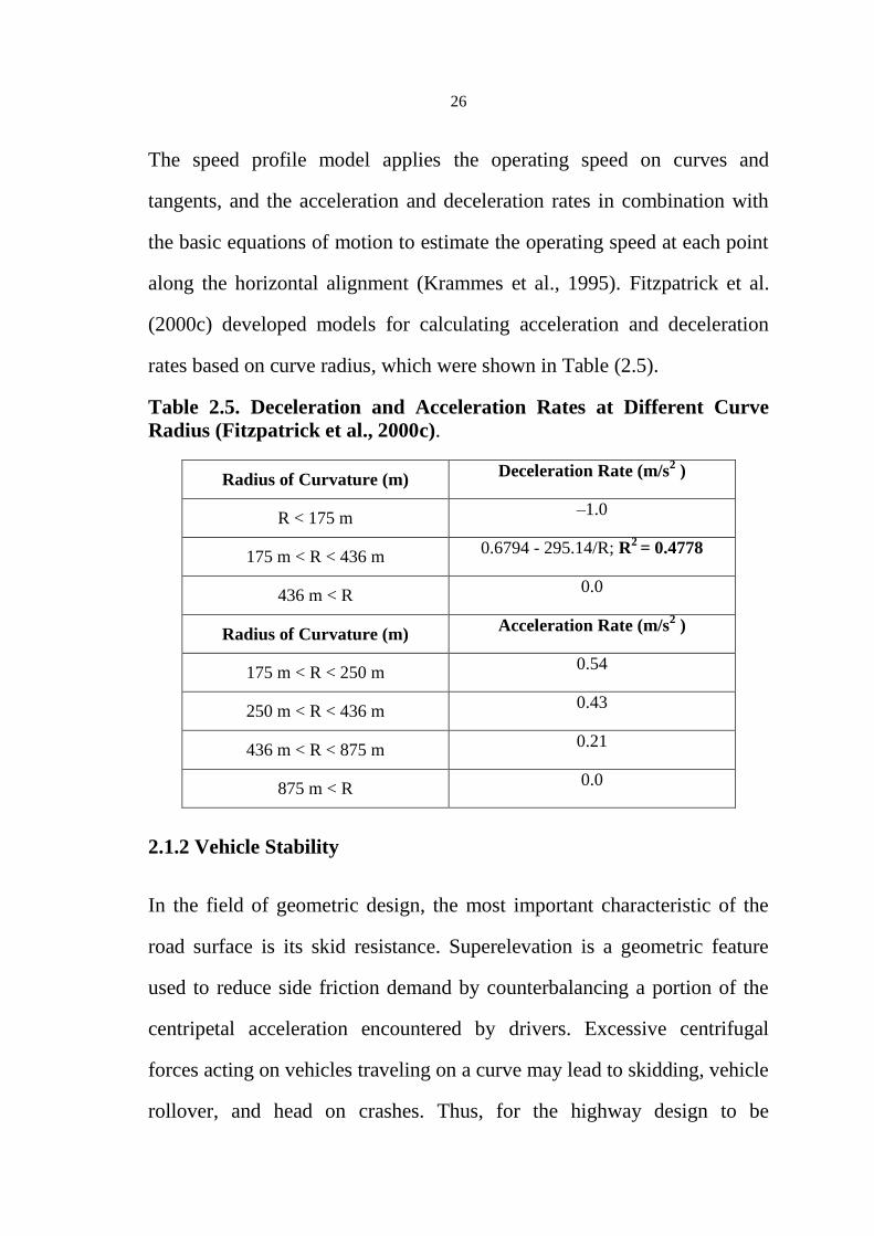
The speed profile model applies the operating speed on curves and

tangents, and the acceleration and deceleration rates in combination with

the basic equations of motion to estimate the operating speed at each point

along the horizontal alignment (Krammes et al., 1995). Fitzpatrick et al.

(2000c) developed models for calculating acceleration and deceleration

rates based on curve radius, which were shown in Table (2.5).

Table 2.5. Deceleration and Acceleration Rates at Different Curve

Radius (Fitzpatrick et al., 2000c).

Radius of Curvature (m) Deceleration Rate (m/s

2 )

R < 175 m –1.0

175 m < R < 436 m 0.6794 - 295.14/R; R

2 = 0.4778

436 m < R 0.0

Radius of Curvature (m) Acceleration Rate (m/s

2 )

175 m < R < 250 m 0.54

250 m < R < 436 m 0.43

436 m < R < 875 m 0.21

875 m < R 0.0

2.1.2 Vehicle Stability

In the field of geometric design, the most important characteristic of the

road surface is its skid resistance. Superelevation is a geometric feature

used to reduce side friction demand by counterbalancing a portion of the

centripetal acceleration encountered by drivers. Excessive centrifugal

forces acting on vehicles traveling on a curve may lead to skidding, vehicle

rollover, and head on crashes. Thus, for the highway design to be

27

consistent and ensure a level of vehicle stability and driver comfort, it

should supply the side friction demanded to balance centrifugal forces.

McLean (1976) stated that side friction is fundamental to curve design, but

that the “design values must be based on a realistic assessment of driver

behavior and comfort tolerance of modern drivers”.

The design consistency evaluation can be done based on a margin of safety

of the difference between side friction supply and side friction demand on

a curve (∆fR). If friction demand exceeds supply, this may prohibit safe

vehicle operation and would imply inconsistency and vehicle instability.

Locations that do not provide vehicle stability can be considered geometric

design inconsistencies (Gibreel et al, 1999).


Vehicle Stability

Lamm et al. (1999) presented a design consistency criterion, which

includes the difference between side friction supplied (fS, that depends on

the design speed) and demanded (fD, that depends on the operating speed),

denoted as (∆fR), was used to represent vehicle stability. Criterion

suggested by Lamm et al. (1999) for consistency evaluation was based on

vehicle stability shown hereafter:

1. Good design: ∆fR +0.01 (no improvement is required),

28

2. Fair design: +0.01 ∆fR -0.04 (the superelevation must be related to

the operating speed to ensure that the side friction assumed will

accommodate the side friction demanded),

3. Poor design: ∆fR -0.04 (strong inconsistency; redesign recommended).

Note: ∆fr = difference between side friction supplied and demand

2.1.2.2 Vehicle Stability Prediction Models on Curves

A different approach for measuring side friction factors was adopted in

worldwide. Several models have been developed to predict side friction

supplied and side friction demanded separately.

Side Friction Supplied

Available friction, which is the friction provided by the pavement depends

on the vehicle speed. It has been theoretically established in the model

developed by Pennsylvania State University (Kulakowski, 1991), and it

has also been empirically verified through many experiments, Wambold

and Henry (1995). Such studies showed that skid resistance diminishes as

speed augments, at a nonlinear rate defined by the macro texture of the

pavement. Likewise, it has been verified by Lamm et al. (1999) that show

the decreasing tendency of friction as speed increases. They proposed

relationship for finding relevant side friction factors in highway curve

design. Side friction is directly related to the tangential friction factor as

shown in Equation (2.4) below.

29

fTP = 0.59 - 4.85 x 10-3

x VD + 1.51 x 10-5

x VD2 (2.4)

Where:

fTP = maximum permissible tangential friction factor, and

VD = design speed (km/h).

After the establishment of the relationship between the maximum

permissible tangential friction factor and the design speed, the range from

which the utilization ratio "n" of the maximum permissible side friction

factor shall be selected. Based on international experiences, this value

varies between n = 40% and n = 50% for rural roads. That means that there

will be still 90% and 87%, respectively of friction available in the

tangential direction for acceleration, deceleration, braking, or evasive

maneuvers when driving through curves (Lamm, 1984). Thus, the equation

for the maximum permissible side friction factor is:

fRPerm. = n x 0.925 x fTP (2.5)

Where:

fRPerm. = maximum permissible side friction factor,

n = utilization ratio, and

0.925 = reduction factor corresponds to tire-specific influences.

Based on Lamm et al. (1994) specific topographic conditions (flat, hilly

and mountainous topography) different utilization ratios were considered

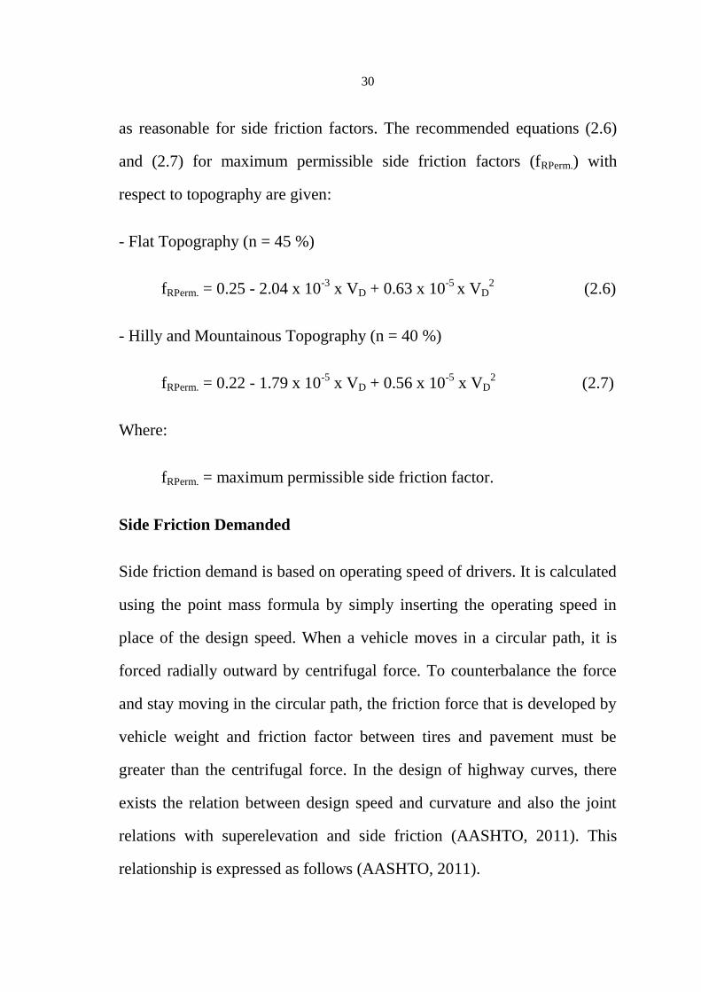
30

as reasonable for side friction factors. The recommended equations (2.6)

and (2.7) for maximum permissible side friction factors (fRPerm.) with

respect to topography are given:

- Flat Topography (n = 45 %)

fRPerm. = 0.25 - 2.04 x 10-3

x VD + 0.63 x 10-5

x VD2

(2.6)

- Hilly and Mountainous Topography (n = 40 %)

fRPerm. = 0.22 - 1.79 x 10-5

x VD + 0.56 x 10-5

x VD2 (2.7)

Where:

fRPerm. = maximum permissible side friction factor.

Side Friction Demanded

Side friction demand is based on operating speed of drivers. It is calculated

using the point mass formula by simply inserting the operating speed in

place of the design speed. When a vehicle moves in a circular path, it is

forced radially outward by centrifugal force. To counterbalance the force

and stay moving in the circular path, the friction force that is developed by

vehicle weight and friction factor between tires and pavement must be

greater than the centrifugal force. In the design of highway curves, there

exists the relation between design speed and curvature and also the joint

relations with superelevation and side friction (AASHTO, 2011). This

relationship is expressed as follows (AASHTO, 2011).

31

fr + e = V852 / 127 R (2.8)

Where:

fr = coefficient of side friction,

e = superelevation rate (m/ m),

V85 = operating speed (km/h), and

R = radius of horizontal curve (m).

Lamm et al. (1991) observed vehicle speeds on curves and used equation

(2.8) to calculate the amount of friction demanded. Bonneson (2001)

developed a side friction prediction model based on the hypothesis that

drivers will modify their side friction demand to achieve a combination of

safe and efficient travel. Bonneson's model was mainly based on the

approach speed and operating speed reduction of a curve. The form of the

model is as follows:

fD = 0.256 - 0.0022 Va + B x (Va - Vc), R2 = 0.88 (2.9)

Vc = 63.5 x (-B (B2 +4c/(127R)

0.5) Va (2.10)

With

c = e/100 + 0.256 + (B - 0.0022) x Va (2.11)

B = 0.0133 - 0.00741 x TR (2.12)

Where:

32

fD = side friction demanded,

Va = 85th

percentile approach speed (km/h),

Vc = 85th

percentile curve speed (km/h),

e = super elevation rate (percent), and

TR = indicator variable (=1.0 for turning roadways; 0.0 otherwise).

2.1.3 Alignment Indices

Alignment indices are quantitative measures of the general character of a

highway segment’s alignment (Anderson et al, 1999). They are not subject

to any evaluation criteria; however, it is noted that geometric

inconsistencies will occur when the general character of an alignment

changes significantly (Hassan et al, 2001, and Fitzpatrick et al, 2000a).

2.1.3.1 Identification of Alignment Indices

Determining the alignment indices consisted of identifying all possible

indices that may be useful for this study. Therefore, some of the alignment

indices that had been used in other countries or proposed for use were

included. All of these alignment indices could possibly provide an

indication of the geometry motorists experience on the roadway.

33

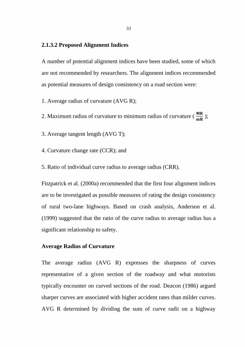
2.1.3.2 Proposed Alignment Indices

A number of potential alignment indices have been studied, some of which

are not recommended by researchers. The alignment indices recommended

as potential measures of design consistency on a road section were:

1. Average radius of curvature (AVG R);

2. Maximum radius of curvature to minimum radius of curvature (

);

3. Average tangent length (AVG T);

4. Curvature change rate (CCR); and

5. Ratio of individual curve radius to average radius (CRR).

Fitzpatrick et al. (2000a) recommended that the first four alignment indices

are to be investigated as possible measures of rating the design consistency

of rural two-lane highways. Based on crash analysis, Anderson et al.

(1999) suggested that the ratio of the curve radius to average radius has a

significant relationship to safety.

Average Radius of Curvature

The average radius (AVG R) expresses the sharpness of curves

representative of a given section of the roadway and what motorists

typically encounter on curved sections of the road. Deacon (1986) argued

sharper curves are associated with higher accident rates than milder curves.

AVG R determined by dividing the sum of curve radii on a highway

34

section by the number of curves on that section as shown in Equation

(2.13).

AVG R (m) = ( Ri) / n (2.13)

Where:

Ri = radius of curve (m), and

n = number of curves within section.

Ratio of Maximum Radius to Minimum Radius

The range of the radii along a roadway can be determined by computing

the ratio of the maximum to minimum radius (

). This ratio can

represent “the consistency of the design in terms of the use of similar

horizontal radii along the road. As this value approaches one, a reduced

accident rate may be expected” (Polus, 1980). Anderson et al. (1999)

stated that the ratio of the maximum radius to the minimum radius is not

recommended as a design consistency measure due to its relatively low

sensitivity to crash frequency compared to other alignment indices studied.

Fitzpatrick et al. (2000a) recommended that a better using the average

radius as an alignment index rather than the maximum radius to minimum

radius. Maximum radius to minimum radius is calculated as follows in

Equation (2.14).

= Rmax / Rmin

(2.14) Where: Rmax = the maximum radius of a highway section, and

35

Rmin = the minimum radius of a highway section.

Average Tangent Length

If a tangent is long enough, then motorists will drive at their desired speed,

which is defined as “the speed at which drivers choose to travel under free-

flow conditions when they are not constrained by alignment features”

(McLean, 1981). Therefore, if motorists are driving at a high speed on the

tangent and a large reduction in speed is required at the following curve,

they may not be able to decrease their speed as needed (Fitzpatrick et al,

2000a). The average tangent length (AVG T) indicates the length of

tangent that is typically available to motorists between curved sections of

the roadway. Average tangent is calculated as follows in Equation (2.15).

AVG T (m) = ( Ti) / n (2.15)

Where:

Ti = tangent length (m), and

n = number of tangents within section.

Curvature Change Rate

Curvature change rate (CCR) expresses the absolute sum of the angular

changes in the horizontal alignment divided by the length of the highway

section (Fitzpatrick et al, 2000a). This parameter assumed to be more

representative of the general character of the alignment of the roadway, a

36

large value for this index indicates that the road either contains a large

number of curves or there are long or sharp curves in that section. It was

expected that an increase in the value of these indices would decrease the

desired speeds of motorists (Fitzpatrick et al, 2000b). Curvature change

rate is calculated as follows in Equation (2.16).

CCR (deg./km) = ( Δi) / Li (2.16)

Where: i = deflection angle (deg), and

Li = length of section (km).

Chen et al. (2011) found that the CRR is a more appropriate value to

describe the geometric properties of several elements. In general, a higher

CRR is associated with higher accident rate.

Curve Radius to Average Radius

The CRR characterizes the relationship between each individual horizontal

curve radius to the average radius of the roadway section as a whole.

Anderson et al. (1999) found that highway safety is sensitive to CRR and

suggested using this ratio as a consistency measure. When the radius of a

horizontal curve deviates greatly from the average radius along the

roadway section, that curve may violate driver expectancy, creating

inconsistency. The ratio CRR for specific curve can be calculated as in

Equation (2.17).

37

CRRi = Ri / AVG R (2.17)

Where:

Ri = radius of the ith curve on the roadway section (m), and

AVG R = Average Radius (m).

The ratio CRR as the value approaches 1.0, a reduced crash frequency is

expected. A curve with a CRR value of 0.5 will be considered by many to

have a relatively higher potential for crashes.

2.1.4 Driver Workload

Messer (1980) defined driver workload as “the time rate at which drivers

must perform a given amount of work or driving tasks”. He indicated that

driver workload increases with reductions in sight distance and increasing

complexity of geometric features, as the complexity of highway geometric

features increases, the time rate required to perform a given driving task is

expected to increase also, consequently reflecting higher driver workload.

Mental workload can be generally defined as the expenditure of mental

capacity required when performing a task or a combination of tasks. How

the driving task is performed is influenced by driver mental characteristics

including expectancy, attention level, and mental workload capacity

(Heger, 1998). Consistent roadway geometry allows a driver to accurately

predict the correct path while using little visual information processing

38

capacity, thus allowing attention or capacity to be dedicated to obstacle

avoidance and navigation (Fitzpatrick et al., 2000d).

It was found that locations with high driver workload values tended to

experience higher crash frequency due to driver confusion or overload

resulting in dangerous reactions to roadway situations. On the other hand,

highway sections with extremely low driver workloads may cause driver

boredom and less concentration on the road (Wooldridge, 1994). Thus,

geometric features resulting in extremely high or low driver workloads

should be avoided to improve road consistency.

There is a strong relationship between crashes, roadway-based geometric

inconsistency, and driver workload (Messer, 1980); drivers who fail to

identify the disparity between their expectation and the actual workload

level may make speed or path errors, consequently increasing their crash

risk (Krammes et al., 1995).

Driver workload is not easily measurable by analytical models; however,

several methods have been developed to quantify the effects of design

consistency on driver workload. In general, workload measurement

techniques fit into five broad categories: primary task measurement,

secondary task measurement, subjective rating, physiological measure, and

visual occlusion.

39

2.1.4.1 Primary Task Measurement

In a primary task measurement the operator performs a task, and some

aspect of the task is varied to increase task loading (e.g., for steering a car,

the mean and variance of a cross wind is increased).

2.1.4.2 Secondary Task Measurement

In a secondary task measurement, the operator performs two tasks: the

primary task, the operational task of interest (steering, for a car), and a

secondary task which is imposed to occupy the part of the operator's

"capacity" not required by the primary task

2.1.4.3 Subjective Rating

A subjective rating scale has been developed by Messer (1980) to estimate

the average workload and the level of consistency of nine basic geometric

roadway features: bridges, divided highway transitions, lane drops,

intersections, railroad grade crossings, shoulder width changes, alignment,

lane width reductions, and the presence of cross road overpasses.

2.1.4.4 Physiological Measure

Several noninvasive physiological measurements are thought to measure

aspects of operator state that correlate with the ability to perform tasks.

Wierwille and Eggemeier (1993) identify the most widely used

measurements to be heart rate (HR), heart rate variability (HRV), brain

activity, and eye activity.

40

2.1.4.5 Visual Occlusion

Vision occlusion was used to determine the effective workload on the

driver under the assumption that the driver only needs to observe the

roadway part of the time, this method blanks out the driver’s vision of the

roadway using a visor or other similar device. By measuring the amount of

time the driver is viewing the roadway, a measure of the information load

of the driver is obtained. This measure of workload, termed visual demand

(VD), has been found to increase as the difficulty of driving increases.

Thus, Vision occlusion is a technique that measures driver visual demand

on a roadway.

Visual demand was defined as the amount of visual information needed by

the driver to maintain an acceptable path on the roadway (Wooldridge et.

al, 2000). Visual demand reflects the percentage of time that a driver is

observing the roadway and is measured using a vision occlusion

procedure. During the procedure, drivers wore an LCD visor that was

opaque except when the driver requested a 0.5-second glimpse through the

use of a floor-mounted switch. Visual demand was measured as the ratio of

the glimpse length divided by the time elapsed from the last glimpse until

the time of the present request (Fitzpatrick et al., 2000a).

Fitzpatrick et al., (2000a) recommended simulator results, which can

provide reasonable estimates of real world estimates of workload and

should be considered for use in future studies of visual demand. Simulator

study size was 24 drivers, 6 repetitions per curve per driver. The authors

41

developed two different regression models for visual demand based on

Simulator study. One model represents drivers familiar with the road

(VDLF), while the other represents drivers unfamiliar with the road (VDLU):

VDLF = 0.388 + 34.7 (2.18)

VDLU = 0.367 + 36.5 (2.19)

Where:

VDLF = visual demand of familiar drivers,

VDLU = visual demand of unfamiliar drivers, and

R = radius of curvature (m).

Visual demand increases linearly with the inverse of radius. That is, as

radius becomes smaller, visual demand increases. Wooldridge et al. (2000)

recommended the use of visual demand as a measure of consistency.

2.2 Relationships of Consistency Measures to Safety

Geometric design consistency is emerging as an important component in

highway design (Glennon et al. 1978). Some researchers have explicitly

noted that treating any inconsistency in a highway alignment can

significantly improve its safety performance (Joanne and Sayed, 2004). A

criterion has been suggested by Lamm et al. (1987) to evaluate design

consistency based on crash rates, the crash rates should correspond to

certain ranges:

42

1. Good design: Cr.Rate ≤ 2.27,

2. Fair design: 2.27 Cr.Rate ≤ 5.00,

3. Poor design: Cr.Rate 5.00.

Note: Cr.Rate = mean crash rate (crash / 106 veh-km).

Joanne and Sayed (2004) investigated the effects of several design

consistency measures on safety. The design consistency measures

mentioned were difference between the 85th percentile operating speed

and design speed (V85 - VD), speed reduction (∆V85), difference between

side friction supplied and side friction demanded on a curve (∆fR), the ratio

of the curve radius to average radius (CRR) and visual demand (VD).

Anderson et al. (1999) investigated the relationship between design

consistency and safety using log linear regression models. Two models

were developed relating accident frequency to traffic volume, curve length,

and speed reduction (∆V85). A separate model was developed relating

accident frequency to curve length and the ratio of the curve radius to

average radius (CRR). He suggested that CRR has a significant

relationship to safety.

Polus (1980) investigated the relationship between longitudinal geometric

measures (such as the average radius, or the ratio between the minimum

and maximum radius of an alignment) and safety levels on two-lane rural

highways and proposed that safety correlated with consistency.

43

Easa (2003) presented a method to distribute superelevation to maximize

highway-design consistency based on safety margins defined as the

difference between the maximum-limit safe speed and the design speed.

Analyses of crashes on the two-lane rural highways have shown that a

significant relationship exists between crash frequency and alignment

indices, which are quantitative measures of the general character of an

alignment in a section of road. Alignment indices include average radius

(AR), ratio of maximum to minimum radius (

), average rate of vertical

curvature (AVC) and the CRR (Hassan, 2004).

Cafiso et al. (2007) presented a methodological approach for the safety

evaluation of two-lane rural highway segments that uses both analytical

procedures referring to alignment design consistency models and safety

inspection processes. They developed a safety index (SI) that

quantitatively measures the relative safety performance of a road segment.

The SI is formulated by combining three components of risk: the exposure

of road users to road hazards, the probability of a vehicle being involved in

an accident, and the resulting consequences should an accident occur.

2.3 Previously Developed Crash Prediction Models

Vogt and Bared (1998) developed a model for predicting the safety

performance of road sections on two-lane rural highways. The model is

shown below in US customary units:

44

Nbr = EXPO x exp(0.6409 + 0.1388STATE - 0.0846LW - 0.0591SW +

0.0668RHR + 0.0084DD ) x ( ∑WHi x exp(0.0450DEGi) ) x ( ∑WVj x exp

(0.4652Vi) ) x ( ∑WGi x exp(0.1048GRi) (2.20)

Where:

Nbr = predicted number of total accidents per year on a particular roadway

segment.

EXPO = exposure in million vehicle-miles of travel per year =

(ADT)(365)(L)(10-6

),

ADT = average daily traffic volume (veh/day) on roadway segment,

L = length of roadway segment (mi),

STATE = location of roadway segment (0 in Minnesota, 1 in Washington),

LW = lane width (ft); average lane width if the two directions of travel

differ,

SW = shoulder width (ft); average shoulder width if the two directions of

travel differ,

RHR = roadside hazard rating; this measure takes integer values from 1 to

7 and represents the average level of hazard in the roadside

environment along the roadway segment,

DD = driveway density (driveways per mi) on the roadway segment,

45

WHi = weight factor for the ith horizontal curve in the roadway segment;

the proportion of the total roadway segment length represented by the

portion of the ith horizontal curve that lies within the segment. (The

weights, WHi, must sum to 1.0.),

DEGi = degree of curvature for the ith horizontal curve in the roadway

segment (degrees per 100 ft),

WVj = weight factor for the jth crest vertical curve in the roadway

segment; the proportion of the total roadway segment length

represented by the portion of the jth crest vertical curve that lies

within the segment. (The weights, WVj, must sum to 1.0.),

Vj = crest vertical curve grade rate for the jth crest vertical curve within

the roadway segment in percent change in grade per 31 m (100 ft) =

|gj2 - gj1| / lj,

gjl, gj2 = roadway grades at the beginning and end of the jth vertical curve

(percent),

lj = length of the jth vertical curve (in hundreds of feet),

WGk = weight factor for the kth straight grade segment; the proportion of

the total roadway segment length represented by the portion of the

kth straight grade segment that lies within the segment. (The weights,

WGk, must sum to 1.0.); and

46

GRk = absolute value of grade for the kth straight grade on the segment

(percent).

This model was developed with negative binomial regression analysis for

data from 619 rural two-lane highway segments in Minnesota and 712

roadway segments in Washington. These roadway segments including

approximately 1,130 km of two-lane roadways in Minnesota and 850 km

of roadways in Washington.

Joanne and Sayed (2004) conducted a study to quantify the safety benefits

of each of the consistency measures presented in this study based on 319

horizontal curves and 511 tangents located in the province of British

Colombia, Canada. The models are as follows:

Cr./5yrs = exp(-3.369) x L0.8858

x V0.5841

x exp[ 0.0049 x (V85 - VD)

+0.0253∆V85 -1.177∆fR (2.21)

Cr./5yrs = exp(-2.338) x L1.092

x V0.4629

x exp[ IC x (0.022 x ∆V85

- 1.189∆fR)] (2.22)

Where:

Cr./5yrs = predicted crash frequency per 5 years,

L = length of section (km),

V = average annual daily traffic (veh/day),

47

V85 - VD = difference between the 85th percentile operating speed

and design speed,

∆V85 = speed reduction between tangent and curve (km/h),

∆fR = difference between side friction supplied and side friction

demanded on a curve, and

IC = dummy variable (IC = 0 for tangents or IC = 1 for horizontal

curves).

Equation (2.22) was developed based on horizontal curves data only while

Equation (2.23) was developed based on both horizontal curves and

tangents. Both models were statistically significant at the 10% significance

level.

The followings model is a sample that shows the relationship between

consistency measures and crash rate (Hassan et al, 2001):

CR = 5.078*10-9

exp(ΔV85) – 8.386 exp(∆fR) + 8.024 exp(VDLU)

(R2 = 0.954) (2.23)

Where:

CR = crash / million vehicle-km,

ΔV85 = differences between V85 on consecutive highway elements,

∆fR = difference between side friction assumed and demanded,

48

VDLU = visual demand of unfamiliar drivers,

R2

= coefficient of multiple correlation.

The authors concluded that the model could be used as a basis for selecting

the proper alignment out of alternatives for two-lane rural highways.

2.4 Summary

Several measures of geometric design consistency have been identified in

the literature and can be classified into four main categories: operating

speed, vehicle stability, alignment indices, and driver workload. Models,

which can be used to estimate these measures and design consistency

evaluation criteria, have been presented.

This chapter provides a review of potential measures of geometric design

consistency and its relationship to road safety. It also provides a review of

some models used for predicting consistency measures and corresponding

evaluation criteria beside previously developed crash prediction models.

Finally, the objectives of this study include investigating and quantifying

the relationship between design consistency and road safety, as well as

estimating the safety benefits of implementing a consistent design.

Specifically, the relationships between various measures of design

consistency and road safety in terms of expected crash occurrence are to be

studied.

http://en.wikipedia.org/wiki/Coefficient_of_multiple_correlation

49

Chapter Three

Research Methodology

The methodology used in this research is based on the development of

Crash Prediction Models (CPM) incorporating design consistency

measures.

3.1 Literature Review

Literature review provides a review for potential measures of geometric

design consistency and their relationships to road safety. It also provides a

review of some models used for predicting consistency measures and

corresponding evaluation criteria.

3.2 Data Collection

Data collection provides a detailed description of the database developed

in this study for model development. Population of selected highways is

introduced, in addition to the sources from which data were obtained and

an outline of the main data variables collected. Subsequently, the

collection of the horizontal alignment, traffic volume, crash data, design

speed, and operating speed are introduced.

3.3 Modeling Methodology

The methodology used in this study is based on the development of Crash

Prediction Models (CPM) incorporating design consistency measures. The

50

generalized linear regression modeling (GLM) approach is adopted for

model development.

3.3.1 Selection of Analysis Sites

Because the available database was limited, a careful review was required

to select sections that were suitable for analysis. A minimum section length

of 4 miles and a maximum section length of 20 miles were established for

this analysis. These minimum and maximum section lengths were

primarily intended to make the database appropriate for the analysis of

roadway alignment indices. Fitzpatrick et al., 2000b concluded that

sections shorter than 6.4 km (4 miles) might not provide enough individual

geometric features to compute a representative value of the alignment

indices. Furthermore, sections longer than 32 km (20 miles) might be so

varied that no single value of an alignment index would be representative

of the section as a whole. Therefore, these constraints were adopted in this

study.

Based on reviewing the data for each route and eliminating portions of the

roadway with features that might interfere and affect the accuracy of the

analysis, the following constraints were imposed for the selection of

highway segments:

Rural area: all locations near town or built up area were eliminated

(not rural; out of scope).

51

All locations within 50 m of an intersection were eliminated

(intersection area).

Marked and paved roadways with constant lane width were chosen

(uniform section).

No recent roadway improvements (no change in geometry).

All locations within 100m of an Israeli Military checkpoint were

eliminated (disturbance of normal traffic flow).

Horizontal curves with radius 100 m were eliminated and those

with curve radius 1000 m length were treated as tangents (based

on recommendations of previous research; Awatta, 2003).

These criteria generally attempt to eliminate features that may inhibit an

accurate analysis, and are mostly based on an understanding of the impact

of different roadway features on safety (Awatta, 2003). For example,

although crashes may occur at curves with radius less than 100 m, but

these were not considered as they might be directly related to the

geometric feature of that curve (sharp curve) and not necessarily the design

consistency aspect of it. Segments were also subdivided at intersections

with major changes in average daily traffic (ADT). The remaining

segments that were less than 6.4 km (4 miles) in length were then

discarded and roadway segments more than 32 km (20 miles) in length

were subdivided.

52

3.3.2 Horizontal Alignment

The horizontal alignment data were extracted from drawing the centerline

of the road segments using aerial photograph (year 2012) for the West

Bank. The data obtained from drawing includes: the stations at the

beginning of the curve (PC); the end of the curve (PT); the radius of

curvature; and the length of curve; in addition to the approach and

departure tangent lengths associated with each curve. Highway numbers

and classification information were obtained from the Israeli Central

Bureau of Statistics (ICBS) because most of the rural-highways roads are

located in area (C), which is out of control the Palestinian National

Authority. Therefore, limited data is available for those highways from

Palestinian sources. Traffic volumes (ADT) were obtained from in situ

traffic counts, traffic counted by students work at An-Najah National

University, and the ICBS.

3.3.3 Statistical Analysis

Statistical analysis used in model development is based on the

development of crash prediction models incorporating design consistency

measures. Crash prediction model (CPM) is an appropriate approach to

evaluate the safety performance of a location. The generalized linear

regression modeling (GLM) approach is adopted for model development.

The GLM has the advantage of overcoming the limitations associated with

the use of conventional linear regression in modeling crash occurrence,

which is random, discrete, and non-negative in nature. Furthermore, GLM

53

has the flexibility of assuming different error distributions and link

functions that allow the conversion of nonlinear models into linear models.

For the GLM approach, the error structure that best fits the crash

occurrence is usually assumed to be Poisson or Negative Binomial. It is

important to understand that neither the Poisson nor Negative Binomial

approach is always best. The selection of either regression technique

should always be based on an analysis of the data under study.

3.3.4 Estimating Consistency Measures

Relationships between road safety and each of the four categories of

geometric design consistency measures: operating speed, vehicle stability,

alignment indices, and driver workload are studied. The measures selected

to represent each category and the corresponding methods used will be

estimated as described below.

3.3.4.1 Operating Speed

The difference between operating speed and design speed (V85 - VD) and

the speed reduction between two successive elements (∆V85) are used. The

operating speed on curves and tangents (V85) was estimated using Google

Earth maps, real time traffic data were obtained from the maps, a spot

speed measurements for tangents and curves are usually collected, as

explained in section (4.6).

The traffic data on Google Maps comes from users of Google Maps for

mobile phone who contribute anonymous speed information through traffic

54

crowd sourcing feature regardless of who they are; Palestinians or others.

A minimum of thirty spot speed measurements for tangents and curves

were collected. Speed data were useful for studying the actual operating

speed with regard to acceleration/declaration behavior.

The design speed for the studied highways was calculated depending on

the speed limit, which has been explained in section (4.6).

The 85th

percentile of the speed reductions from tangent to curve or from

two successive curves (∆V85) were calculated depending on Abdelwahab et

al. (1998) model to predict speed reduction shown in Equation (2.1).

3.3.4.2 Vehicle Stability

The difference between side friction supplied (fS, that depends on the

design speed) and demanded (fD, that depends on the operating speed),

denoted as (∆fR), was used to represent vehicle stability. If friction demand

exceeds supply, this may prohibit safe vehicle operation and would imply

inconsistency and vehicle instability. Thus, vehicle stability on horizontal

curves is paramount in ensuring road safety.

Side friction supplied is based on operating speed of highway sections.

Lamm et al. (1999) proposed relationship for finding relevant side friction

demand factors in highway curve design, based on Lamm et al. (1994)

specific topographic conditions (flat, hilly and mountainous topography)

different utilization ratios were considered as reasonable for side friction

factors. The recommended Equations (2.6) and (2.7) for maximum

55

permissible side friction factors (fRPerm.) with respect to topography are

given as explained in section (2.1.2.2).

Bonneson (2001) developed a side friction prediction model based on the

hypothesis that drivers will modify their side friction demand to achieve a

combination of safe and efficient travel. Bonneson's model was mainly

based on the approach speed and operating speed reduction of a curve.

Used with the allowed speed reduction, this model can provide the

maximum allowable side friction for the design of critical design control

elements. The model form is shown in Equations (2.9, 10, 11, and 12), as

explained in section (2.1.2).

3.3.4.3 Alignment Indices

Alignment indices are quantitative measures of the general character of a

highway segment’s alignment (Anderson et al, 1999). The alignment

indices recommended as potential measures of design consistency on a

road section were:

1. Average radius of curvature (AVG R);

2. Maximum radius of curvature to minimum radius of curvature

(MR/mR);

3. Average tangent length (AVG T);

4. Curvature change rate (CCR); and

5. Ratio of individual curve radius to average radius (CRR).

AVG R calculated based on equation (2.13), MR/mR is calculated based

on equation (2.14), AVG T is calculated based on equation (2.15), CCR is

56

calculated based on equation (2.16), and CRR is calculated based on

equation (2.17). Alignment indices have been explained in section (2.1.3).

3.3.4.4 Driver Workload

The models, which estimate visual demand of drivers unfamiliar VDLU

(Equation 2.19) and of drivers familiar VDLF (Equation 2.18) with the road

developed by Fitzpatrick et al., (2000a) were adopted. To overcome the

selection between the familiar and unfamiliar visual demand models, only

one of the visual demand models was included in this analysis. The model

predicting visual demand of familiar drivers will be developed because

most of drivers drive regularly or know well the roads.

3.4 Modeling Validation

To evaluate the accuracy of the West Bank crash prediction models (CPM)

developed, a validation step was performed. The goal of this validation

step is not only to compare the accuracy of different models developed, but

also to evaluate the overall accuracy of CPMs for use on rural two-lane

highways in the West Bank.

3.5 Modeling Application

A qualitative comparison has also been made to compare collision

prediction models, which explicitly consider design consistency with those

that rely on geometric design characteristics for predicting collision

occurrence. A systematic approach to identify geometrically inconsistent

locations using the safety consistency factor has been proposed.

57

3.6 Conclusions and Recommendations

The main conclusions are presented and future recommendations are given

at the end of this research.

58

Chapter Four

Data Collection

This chapter provides a detailed description of the database developed in

this study for model development and validation. In section 4.1, the sample

of selected highways is introduced, in addition to the sources from which

data were obtained and an outline of the main data variables collected.

Subsequently, sections 4.2 to 4.6 discuss the collection of the horizontal

alignment, traffic volume, crash data, design speed, and operating speed.

4.1 Overview of Data Collected

Four two-lane rural highway segments located in the West-Bank were

chosen for analysis. The selection of these highways was mainly based on

limitations in data availability. However, it was ensured that the selected

highways encompass a variety of highway classifications, locations,

terrain, design speed, traffic volume, and crash history, hoping that this

sample would cover most of the two-lane rural highway conditions found

in West Bank. Figure (4.1) shows highway locations chosen for analysis in

the West Bank. Horizontal alignment, traffic volume, crashes, design

speed, and operating speed for two-lane rural highway located in West

Bank, Palestine, are used. Summary of selected highways is shown in

Table (4.1).

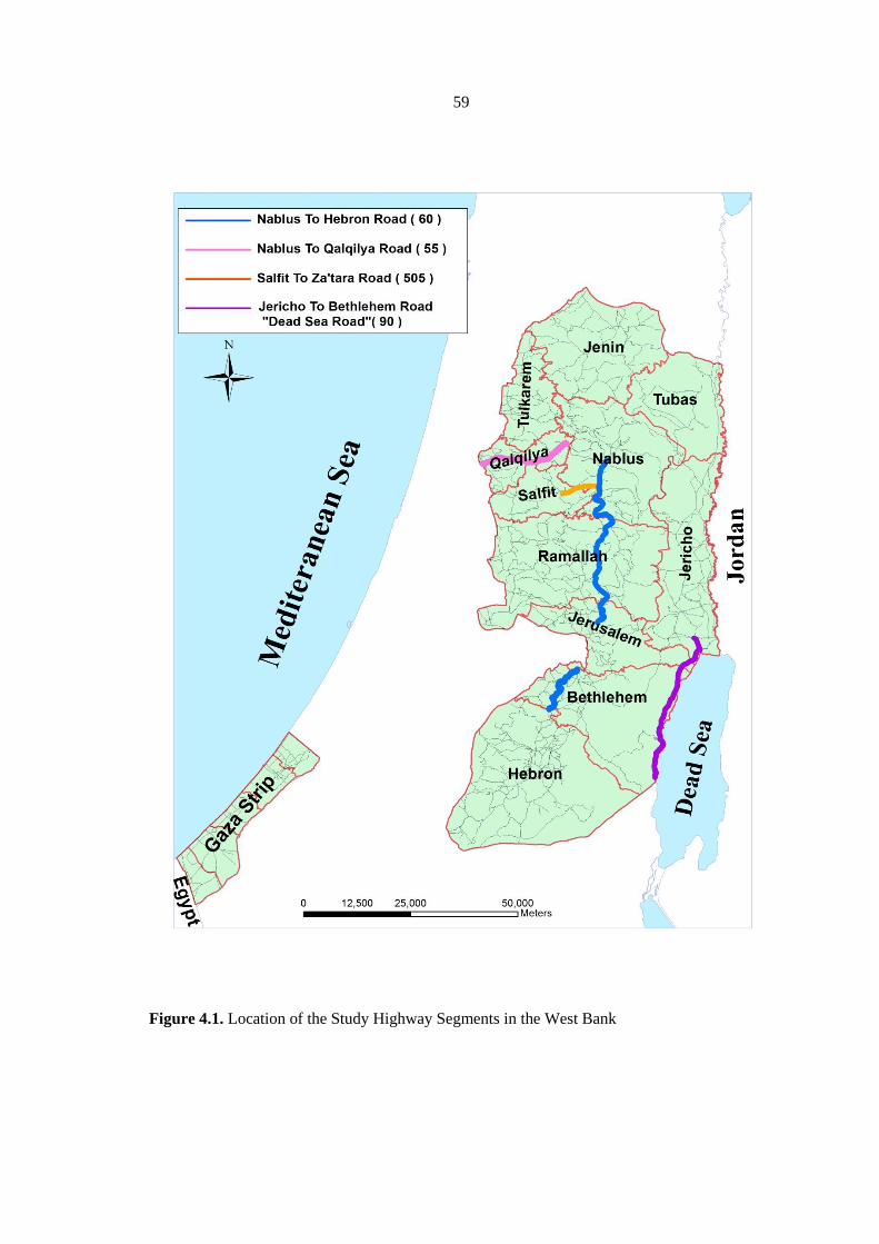
59

Figure 4.1. Location of the Study Highway Segments in the West Bank

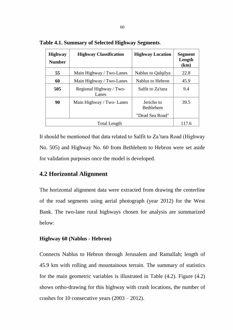
60

Table 4.1. Summary of Selected Highway Segments.

Highway

Number

Highway Classification Highway Location Segment

Length

(km)

55 Main Highway / Two-Lanes Nablus to Qalqilya 22.8

60 Main Highway / Two-Lanes Nablus to Hebron 45.9

505 Regional Highway / Two-

Lanes

Salfit to Za'tara 9.4

90 Main Highway / Two- Lanes Jericho to

Bethlehem

"Dead Sea Road"

39.5

Total Length 117.6

It should be mentioned that data related to Salfit to Za’tara Road (Highway

No. 505) and Highway No. 60 from Bethlehem to Hebron were set aside

for validation purposes once the model is developed.

4.2 Horizontal Alignment

The horizontal alignment data were extracted from drawing the centerline

of the road segments using aerial photograph (year 2012) for the West

Bank. The two-lane rural highways chosen for analysis are summarized

below:

Highway 60 (Nablus - Hebron)

Connects Nablus to Hebron through Jerusalem and Ramallah; length of

45.9 km with rolling and mountainous terrain. The summary of statistics

for the main geometric variables is illustrated in Table (4.2). Figure (4.2)

shows ortho-drawing for this highway with crash locations, the number of

crashes for 10 consecutive years (2003 – 2012).

61

Figure 4.2: Ortho-Drawing for Highway 60 with Accident Locations.

62

Table 4.2. Summary of Statistics for Main Variables Used in Highway

60.

Data Element Minimum Maximum Mean Standard

Deviation

Curve Radius (m)* 231.08 982.14 479.12 180.91

Curve Length (m) 91.2 1687.47 332.05 270.96

Tangent Length (m) 86.12 4905.41 556.87 820.12

* Curves with radius less than 100 m were eliminate from the data

Road section from Nablus to Jerusalem was used for model development

and from Jerusalem to Hebron was used for model validation.

Highway 55 (Nablus to Qalqilya)

Connects Nablus to Qalqilya; road length is 22.8 km with rolling and

mountainous topographic segments. The summary of statistics for the main

geometric variables is illustrated in Table (4.3). Figure (4.3) shows ortho-

drawing for Highway 55 with crash locations along the highway segments,

the number of crashes for 10 consecutive years, 2003 through 2012.

Table 4.3. Summary Statistics for Main Variables Used in Highway

55.


Deviation

Curve Radius (m) * 108.7 988.84 415.10 249.8

Curve Length (m) 61.03 625.21 225.27 159.48

Tangent Length (m) 65.52 2163.89 432.97 544.14


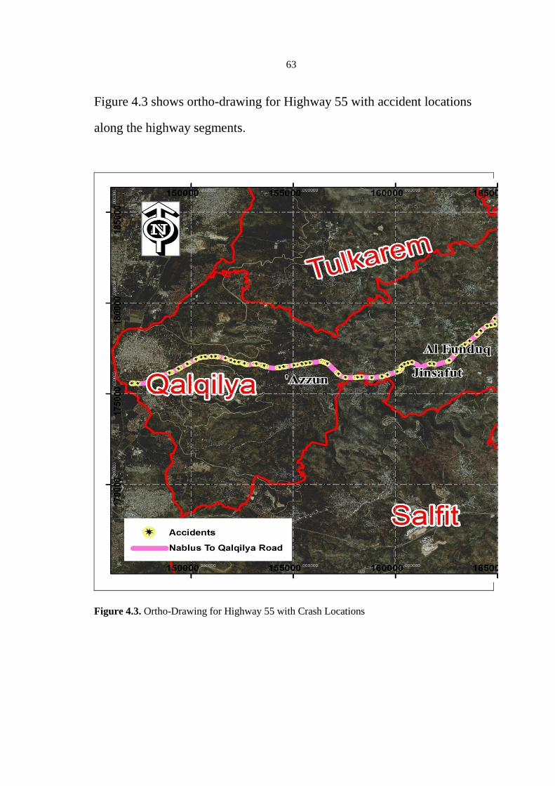
63

Figure 4.3 shows ortho-drawing for Highway 55 with accident locations

along the highway segments.

Figure 4.3. Ortho-Drawing for Highway 55 with Crash Locations

64

Highway 505 (Salfit to Za'tara)

Connects Za’tara to Salfit; road length is 9.4 km with rolling topographic

segments. The summary of statistics for the main geometric variables is

illustrated in Table (3.4). Figure (3.4) shows ortho-drawing for Highway

505 with crash locations along the highway segments, the number of

crashes for 5 consecutive years, 2008 through 2012. Road section from

Salfit to Za'tara used for model validation.


505.


Deviation

Curve Radius (m) * 331.26 985.42 685.41 204.16

Curve Length (m) 104.42 854.86 240.44 201.53

Tangent Length (m) 157.77 1656 676.75 556.17


Highway 90 (Jericho to Bethlehem) “Dead Sea Road"

Connects Jericho to Bethlehem Governorate; it is known as the Dead Sea

Road. The road length is 39.5 km with level terrain. The summary of

statistics for the main geometric variables is illustrated in Table (4.5).

Figure (4.5) shows ortho-drawing for Highway 90 with crash locations

along the highway segments, the number of crashes for 10 consecutive

years, 2003 through 2012. Road section from Jericho to Bethlehem used

65

for model development and Bethlehem governorate road section used for

model validation.

Figure 4.4. Ortho-Drawing for Highway 505 with Crash Locations.

66

Figure 4.5. Ortho-Drawing for Highway 90 with Accident Locations.

67


90.

Data element Minimum Maximum Mean Standard

Deviation

Curve Radius (m) * 129.67 937.79 471.32 226.12

Curve Length (m) 59.65 416.69 181.67 70

Tangent Length (m) 77.26 2523.35 443.11 437.41


4.3 Traffic Volume

The traffic volume data for Highway 60 (Nablus to Hebron) were obtained

from Rabaya et. al (2012) study, which provides traffic counts for two

sections along the highway. Highway 55 (Nablus to Qalqilya) traffic

volume data were obtained from in situ traffic count in year (2012) for the

first section, the second section was obtained from the ICBS in year

(2012). Highway 505 (Za'tara to Salfit) traffic volume data were obtained

from in situ traffic count in year 2012. Highway 90 (Jericho to Bethlehem

"Dead Sea Road") traffic volume data were obtained from the ICBS in

year (2012).

Average daily traffic volumes for the studied roads were needed for five

years. Unfortunately, the only data of traffic volume were obtained for one

year from Rabaya et al. (2012) study and from in situ traffic counts,

therefore, it is needed to be expanded for five years (2008-2012) to use in

model development.

68

Although the crashes data does not distinguish between those involving

Palestinian or Israeli settlers, the growth rate for the population in the West

Bank was used to represent the growth rate for vehicle volumes because

the majority of drivers on these highway sections are Palestinians and the

population growth rate for Israeli settlers is different from the Palestinians.

Population and growth rates in the West Bank are illustrated in Table (4.6)

(Palestinian Central Bureau of Statics, 2012).

Table 4.6. Population and Growth Rate in West Bank (PCBS, 2012).

2008 2009 2010 2011 2012

Population 2385180 2448433 2513283 2580168 2649020

Growth Rate 2.65% 2.65% 2.66% 2.67%

The average daily traffic (ADT) for the studied roads were calculated using

population growth rate and K factor (Design Hour Factor) estimated at

15%; values for K typically range from (8-12)% for urban facilities and

(12-18)% for rural facilities (AASHTO, 2001). The K factor allows for the

conversion from a peak hour volume to a daily volume. The ADT for the

studied road sections is illustrated in Table (4.7).

4.4 Crashes Data

The crash data from the ICBS were used to extract 5-year crash experience

of each individual tangent and horizontal curve for (2008- 2012) years.

The crash analysis considers only non-intersection crashes that involved:

69

(1) a single vehicle running off the road; (2) two or more vehicle crash. All

crashes involving parking, hitting pedestrian, and crash with inanimate

object, drop- off elevated pavement, and others were excluded. These are

the crash types that have been identified as being “over-represented on

curves as compared to tangents” (Fitzpatrick et al, 2000b). In addition,

these are crashes that might not be directly related to geometric aspects of

the roads.

Table 4.7. Average Daily Traffic for the Studied Roadway Sections.

Year

Highway

2008 2009 2010 2011 2012 ADT

Veh./Day

60 (Section1)

Nablus Ramallah

10196 10474 10759 11053 11348 10766

60 (Section2)

Ramallah Bethlahem

7122 7316 7515 7715 7920 7518

60 (Section2)

Bethlehem Hebron

12100 14000 12783 11500 9900 12057

55 (Section1)

Nablus Al-Funduq

13700 15100 15200 15500 16300 15160

55 (Section2)

Al-Funduq Qalqilya

2772 2847 2925 3005 3087 2927

505

Za'tara Salfit

2957 3037 3120 3205 3293 3122

90

Jericho Bethlahem

3507 3602 3700 3796 3900 3800

This database contains summarized traffic crash data for all crashes on the

highway sections. Some of the main variables provided by the crash

databases are described below:

Date of crash (year, month, and day of week);

crash coordinate based on the Palestinian grid;

Lighting condition in which crash took place (day and night);

70

Type of crash (head-on crashes, rear-end crashes, side by side

crashes, front-side crashes, skidding, over-turn crashes, ran-off

crashes);

Number of vehicles involved in crashes;

Crash severity (slight, serious, and fatal).

The number of the crashes in the studied highways during 5 years can be

summarized on tangents and horizontal curve locations are illustrated in

Table (4.8), taking into consideration the number of crashes in the table

and excluding all crashes located near town or built up area (urban area),

within 50m of an intersection, and within 100m of an military checkpoints.

It should be noted that the crash date extracted from the ICBS in the Israeli

coordination, which is need to transfer to the Palestinian coordination one

by one, which great effort needed.

Table 4.8. Number of Crashes on Highway Segments During 5 Years.

Highway Number On Tangent On Horizontal Curve Total

55 52 27 79

60 68 66 134

505 14 10 24

90 19 7 26

71

4.5 Design Speed

The Design speed is not known. This value was estimated depending on

the speed limit, which is known for the studied highways. Wooldridge et

al. (2003) presented different considerations to select the design speed

value: AASHTO (2011) consideration of the traditional factors, such as

functional classification and terrain, legal speed limit plus a value (5 to 10

mph [8 to 16 km/h]). Some agencies select design speed values within 0 to

10 mph (0 to 16 km/h) above the legislatively mandated maximum posted

speed limit for the road’s functional classification under consideration.

Others select a design speed value of 5 to 10 mph (8 to 16 km/h) above the

anticipated operating speed. Depending on the previous discussion, 15

km/hr was added to the posted speed limit to estimate the design speed for

the selected highways, as illustrated in Table (4.9).

Table 4.9. Legal Speed Limit and Design Speed for Selected Highways

Highway Number Legal Speed Limit Design Speed

55 80 95

60 90 105

505 80 95

90 90 105

72

4.6 Operating Speed

Operating speed is defined as the speed selected by drivers under free-flow

conditions, commonly taken as the 85th percentile speed, i.e. the speed that

85% of drivers will not exceed (Poe and Mason, 2000). A new approach

had been used to estimate the operating speed (V85) along two-lane rural

roads using Google Earth maps. Real-time speed traffic data were obtained

from the maps. The traffic data on Google Maps comes from a variety of

sources, including governmental departments of transportation, private

data providers, and users of Google Maps for mobile phone who contribute

anonymous speed information through traffic crowd sourcing feature.

Speed data regarding individual car drivers travelling on selected two-lane

rural highways were collected using real-time speed traffic data as show in

Figure (4.6); minimum of thirty spot speed measurements for tangents and

curves were collected then compared with the minimum sample size in

Equation (4.1). Speed data were useful for studying the actual operating

speed with regard to acceleration/declaration behavior.

It should be noted that the speed data using Google Earth Map can be

collected for only those with mobile/GPS-determined locations transmitted

by subscribed users. Also, the speed data was taken during off-peak hours

to represent the free-flow speed, day/night, and for all days of week.

Although the speed sample may be biased towards those using

mobile/GPS-determined locations; however, the data is still considered

representative and is the best available data to compute the actual operating

73

speed. Table (4.10) summarizes operating speeds results for the studied

highway sections.

Table 4.10. Summary of Statistics for Operating Speed Used in the

Studied Highway Sections (in Km/hr).

Highway Location Minimum Maximum Mean Standard

Deviation

Nablus to Qalqilya 46.4 106.3 84.1 10.2

Nablus to Hebron 75.2 115.8 91.5 8.6

Za'tara to Salfit 72 120 99.5 12.8

Jericho to Bethlehem

"Dead Sea Road"

49.6 106.4 84.2 11.7

74

Figure 4.6. Real Time Speed for Individual Car Driver.

Using Equation (4.1), the minimum sample size of spot speed counts

needed for each road segments (tangent and curve) were computed

depending on Z-value of 1.96 (for 95 percent confidence level), the limits

of acceptable error (d) used (depending on the purpose of the study) traffic

operations, economic evaluation, and trend analysis 3.0 to 6 km/hr

(Garber and Hoel, 2009), and standard deviation ( ) computed depending

on the number of spot speed counts, which were already counted in the

75

off-peak hours for each road segments. The spot speed counts for each

road segments must be more than the minimum sample size resulting from

Equation (4.1). The spot speed counts used the study is usually more than

thirty for most locations, which implies that Z-distribution is appropriate

and yields higher than 95% confidence level.

N = (Z 2

) / d2 (4.1)

Where:

N = minimum sample size,

Z = number of the standard deviation corresponding to the required

confidence = level 1.96 for 95 percent confidence

level

= standard deviation (km/hr),

d = limits of acceptable error of the speed estimate (km/hr).

76

Chapter Five

Model Development

The methodology used in model development is based on the development

of crash prediction models incorporating design consistency measures.

Crash prediction model (CPM) is an appropriate approach to evaluate the

safety performance of a location (Sayed and Rodriguez, 1999) which is

explained in Section (5.1). The generalized linear regression modeling

(GLM) approach is adopted for model development, the theoretical basis

and the advantages of are presented in Section (5.2). To develop CPM,

selecting significant variables from numerous candidate variables is a

critical step. The measures selected to represent each category are shown

in Section (5.3).

5.1 Crash Prediction Models

In modern highway safety research, the application of regression analysis

plays a vital role in understanding the impact of roadway features on

safety. Regression models developed for highway safety studies can be

divided into two main uses, crash causation models and crash prediction

models (Persaud, 2001).

Crash prediction models (CPM) are appropriate approach to evaluate the

safety performance of a location. They are statistical regression models

which relate crash occurrence to traffic and geometric characteristics of a

location, and are developed based on a group of locations of similar

77

geometric make-up. The models can be used to predict future crash

occurrence at other locations of similar characteristics (Sayed and

Rodriguez, 1999). Crash prediction models attempt to estimate the

expected crash experience as a function of the strongest predictor

variables, thus there is an emphasis on prediction errors.

5.2 Modeling Techniques

Most of the earlier studies used the conventional linear regression

approach to develop models relating crashes to traffic volumes. However,

the past decades have seen a significant development and advances in

crash data analysis and modeling. Crash prediction models are no longer

limited to conventional linear regression approach, as more accurate and

less restrictive nonlinear models are considered. Jovanis and Chang (1986)

identified three shortcomings associated with the assumption of a normal

distribution error structure. The first shortcoming is found in the

relationship between the mean and the variance of accident frequency,

under a normal distribution assumption, the variance remains constant. The

second shortcoming is associated with the non-negativity of accident

occurrence. The third problem is related with the non-normality of the

error distribution, due to the characteristics of non-negativity and small

value of discrete dependent variable.

To estimate the parameters of crash prediction models, the generalized

linear regression method (GLM) is used. GLM has the advantage of

overcoming the limitations associated with the use of conventional linear

78

regression in modeling crash occurrence, which is random, discrete, and

non-negative in nature. GLM has the flexibility of assuming different error

distributions and link functions that allow the conversion of nonlinear

models into linear models.

5.2.1 Selection of Regression Technique

For the GLM approach, the error structure that best fits the crash

occurrence is usually assumed to be Poisson or Negative Binomial. It is

important to understand that neither the Poisson nor Negative Binomial

approach is always best. The selection of either regression technique

should always be based on an analysis of the data under study.

The main advantage of the Poisson error structure is the simplicity of the

calculations, because the mean and variance are equal. However, this

advantage is also a limitation. It has been shown by Kallberg et al. (1987)

that most accident data is likely to be over dispersed (the variance is

greater than the mean), which indicates that the negative binomial

distribution is the more realistic assumption. The negative binomial

regression technique was then implemented to determine whether it could

accommodate the problem of over-dispersion.

Bonneson and McCoy (1993) proposed a methodology to decide whether

to use a Poisson or Negative Binomial error structure. First, the model

parameters are estimated based on a Poisson distribution error structure.

Secondly, dispersion parameter (k) is calculated depending on scaled

79

deviance (SD) and Pearson Ӽ2. Dispersion parameters are calculated as

follow in Equations (5.1 and 5.2):

kD = SD / n - p (5.1)

kP = Pearson Ӽ2 / n - p (5.2)

Where:

kD = dispersion parameter depending on scaled deviance,

kP = dispersion parameter depending on Pearson Ӽ2,

SD = scaled deviance value of model,

Pearson Ӽ2 = Pearson chi-squared value of model,

n = number of observations,

p = number of coefficients considered in model.

If (k) is greater than 1.0, then the data has greater dispersion than is

explained by the Poisson distribution, and a further analysis using a

Negative Binomial distribution is required. If (k) is near 1.0, then the

assumed error structure approximately fits the Poisson distribution. Scaled

Deviance and Pearson chi-squared measures were provided as SPSS

goodness of fit output (SD and Pearson Ӽ2 test

will be described in Section

5.2.3).

80

5.2.2 Model Structure and Development

Neter et al. (1996) argued that general form typically found in crash

models is the multiplicative model form shown in Equation (5.3). This

multiplicative form ensures zero values of crash frequency at zero values

of the exposure variable. It also ensures that the mean value of crashes

remains positive, since an additive model may result in negative values for

certain parameter combinations.

The model structure relates crashes to exposure and other explanatory

variables such as geometric design features or design consistency

measures. The form of the model equation for negative binomial

regression is the same as that for Poisson regression. The “Ln” of the

outcome is predicted with a linear combination of the predictors, using Ln

as link functions allow the conversion of nonlinear models into linear

models. The following general model forms can be adopted when studying

highway sections:

Ln(Y) = Intercept + β1 ( 1) + β2 ( 2) + β n ( n) (5.3)

This implies:

Y = EXP (Intercept + β

1 (X

1) + β

2 (X

2) + β

n (X

n) =

= EXP (Intercept)

EXP (β

1 (X 1

)

EXP (β

2 (X

2)

EXP (β

n (X

n))

Where:

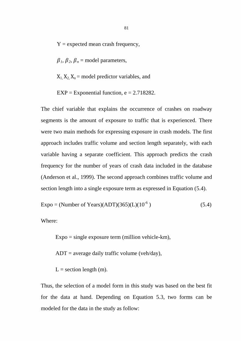
81

Y = expected mean crash frequency,

1, 2, n = model parameters,

1, 2, n = model predictor variables, and

EXP = Exponential function, e = 2.718282.

The chief variable that explains the occurrence of crashes on roadway

segments is the amount of exposure to traffic that is experienced. There

were two main methods for expressing exposure in crash models. The first

approach includes traffic volume and section length separately, with each

variable having a separate coefficient. This approach predicts the crash

frequency for the number of years of crash data included in the database

(Anderson et al., 1999). The second approach combines traffic volume and

section length into a single exposure term as expressed in Equation (5.4).

Expo = (Number of Years)(ADT)(365)(L)(10-6

) (5.4)

Where:

Expo = single exposure term (million vehicle-km),

ADT = average daily traffic volume (veh/day),

L = section length (m).

Thus, the selection of a model form in this study was based on the best fit

for the data at hand. Depending on Equation 5.3, two forms can be

modeled for the data in the study as follow:

82

Y= EXP(Intercept)

EXP ( ADT ( X

1)) EXP

( L ( X 2)) EXP

(β 1( X

3))

000EXP (β

2( X

4)) EXP

(β n(X

n)) (5.5)

Y= EXP (Intercept)

EXP (Expo (X

1)) EXP

(β 1(X

2)) EXP

(β 2(X

3))

000EXP (β

n(X

n))

(5.6)

Where:





L = section length (m),

Expo = single exposure term (million vehicle-km), and


Anderson et al. (1999) examined the two approaches for incorporating

exposure expressed in Equations (5.5) and (5.6), and found that including

the natural logarithms traffic volume and curve length as separate terms

improved the model's goodness of fit. Taking the natural logarithm of the

variables was recommended in previous research. Lovegrove and Sayed

(2006) proposed a generalized linear model form that can be adopted when

83

studying highway sections, which is presented in Equations (5.7) and (5.8)

as:

Y= EXP (Intercept)

ADT(X

1) L(X

2) EXP

(β 1(X

3)) EXP

(β 2(X

4))

EXP (β

n(X

n))

(5.7)

Y= EXP (Intercept)

Expo(X1)

EXP (β

1(X

2)) EXP

(β 2(X

3))

EXP (β

n(X

n))

(5.8)

Where:





L = section length (m),

Expo = single exposure term (million vehicle-km), and


This form not only takes account of the influence of different independent

variables, but also fairly represents the non-negative, non-linear, and non-

normal nature of the crashes. Depending on previous studied, this form

examined and gave reasonable results.

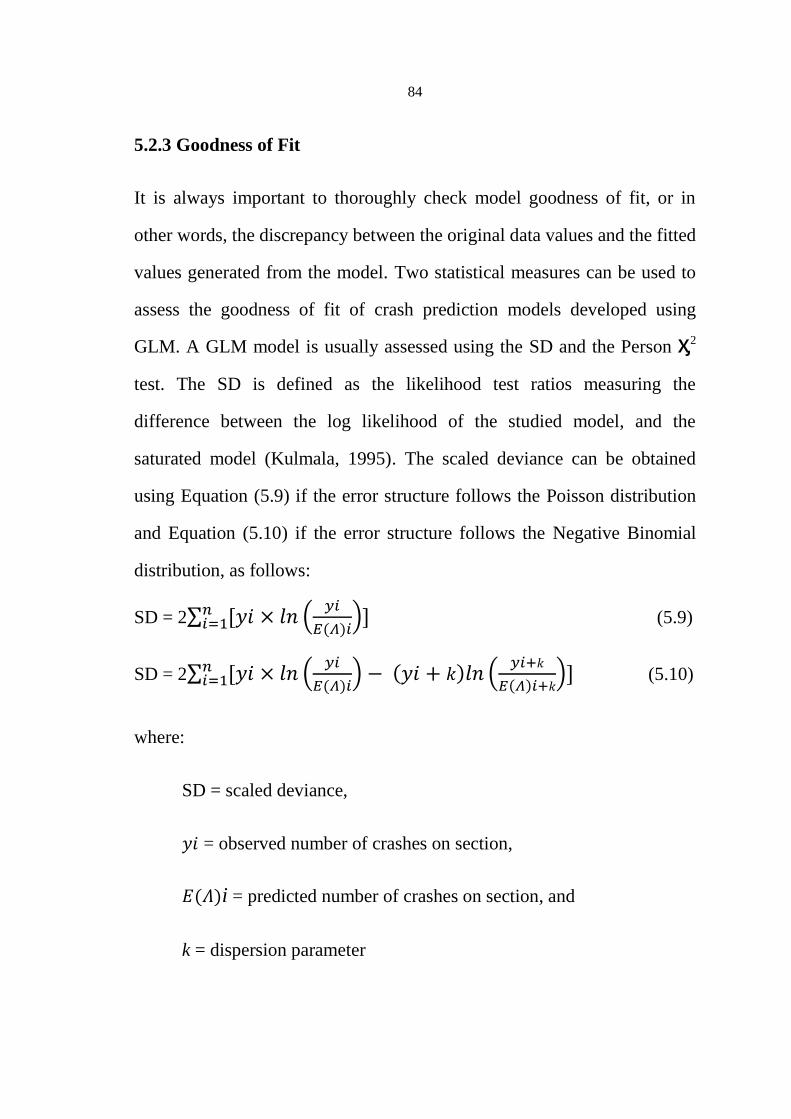
84

5.2.3 Goodness of Fit

It is always important to thoroughly check model goodness of fit, or in

other words, the discrepancy between the original data values and the fitted

values generated from the model. Two statistical measures can be used to

assess the goodness of fit of crash prediction models developed using

GLM. A GLM model is usually assessed using the SD and the Person Ӽ2

test. The SD is defined as the likelihood test ratios measuring the

difference between the log likelihood of the studied model, and the

saturated model (Kulmala, 1995). The scaled deviance can be obtained

using Equation (5.9) if the error structure follows the Poisson distribution

and Equation (5.10) if the error structure follows the Negative Binomial

distribution, as follows:

SD = 2

(5.9)

SD = 2

(5.10)

where:

SD = scaled deviance,

= observed number of crashes on section,

i = predicted number of crashes on section, and

k = dispersion parameter

85

The SD is asymptotically Ӽ2 distributed with n-p-1 degrees of freedom,

where n is the number of observations, and p is the number of model

parameters. Another measure to assess the significance of the GLM

models is the Person Ӽ2 statistics defined as (Bonneson and McCoy, 1993):

Pearson Ӽ2 =

(5.11)

where:

Pearson Ӽ2 = Pearson chi-squared value of model,

= observed number of crashes on section,

i = predicted number of crashes on section, and

= the variance of observed accidents.

The Pearson Ӽ2 statistics follows the Ӽ2

distribution with n-p-1 degrees of

freedom, where n is the number of observations and p is the number of

model parameters. The variance of observed crashes ( ) is defined

in Equations (5.12) and (5.13) for Poisson and negative binomial

distributions, respectively.

= µ; = (µ2 /

k)

(5.12)

= µ; = µ + (µ2 /

k)

(5.13)

86

where:

= µ = average number of crashes on section,

k = dispersion parameter.

The goodness-of-fit statistics for the model shows that the model fits

reasonably well with the data. The Pearson Ӽ2 and SD statistics divided by

its degrees of freedom values must be within the permissible range of (0.8

- 1.2), which indicate that the Negative Binomial distribution assumption is

acceptable (Dissanayeke and Ratnayake, 2006).

The use of the traditional coefficient of determination (R2) is considered

not appropriate for Poisson or Negative Binomial regression models as

goodness of fit measure. Miaou et al. (1995) showed several drawbacks

associated with the use of (R2) for assessing the goodness of fit of crash

prediction models. They proposed another goodness of fit for Negative

binomial models. It is a dispersion based R2, which is calculated as follows

Rk 2 = 1 - kM / kmax (5.14)

where:

Rk 2 = coefficient of determination,

kM = model dispersion parameter, and

kmax = maximum dispersion parameter of the model.

87

Maximum dispersion parameter of the negative binomial distribution is

estimated in the model with only a constant term and no predictor

variables. Maximum dispersion parameter of the model was provided as

SPSS goodness of fit output.

5.3 Selected Consistency Measures

All the design consistency measures mentioned in Chapter 3 (V85 - VD,

∆V85, ∆fR, AVG R, MR/mR, AVG T, CCR, CRR, and VDLF), were

computed for each section of the study highways. Table (5.1) provides a

summary of the design consistency measures as applied to these

alignments. It should be noted that Table (5.1) shows the summary of

statistics for the consistency measures used for highway section used for

model development only.

88

Table 5.1. Summary of Statistics of the Design Consistency Measures

as Applied to the Alignments under Study.

Design Consistency Measure Maximum Minimum Average Std.

Dev

Horizontal Curves Data Only (3 Roads with 136 Horizontal Curves)

V85 - VD (km/hr) 8.59 -47.00 -15.32 -8.59

∆V85 (km/hr) 20.07 2.49 7.21 3.67

∆fR 0.27 -0.13 0.12 0.10

AVG R (m) 509.60 296.9 479.86 57.78

8.60 3.20 5.68 1.78

AVG T (m) 1009.60 182.90 485.15 207.76

CCR 108.60 38.60 55.79 19.08

CRR 2.02 0.23 1.00 0.42

VDLF 0.71 0.42 0.48 0.06

Tangent Data Only (111 Tangents) V85 - VD 11.29 -48.60 -14.33 9.88

Horizontal Curves and Tangents Data Combined (3 Roads with 136 Horizontal


Design Consistency Measure Maximum Minimum Average Std.

Dev

V85 - VD (km/hr) 11.29 -48.60 -14.83 9.19

∆V85 (km/hr) 20.07 0.00 3.96 4.59

∆fR 0.27 -0.13 0.07 0.10

AVG R (m) 509.60 0.00 263.01 243.32

8.60 0.00 3.12 3.11

AVG T (m) 1009.60 0.00 266.39 288.61

CCR 108.60 0.00 30.56 31.43

CRR 2.02 0.00 0.55 0.59

VDLF 0.71 0.00 0.26 0.24

89

Chapter Six

Modeling Results

This chapter presents the models developed in this study. Two groups of

models have been developed with different objectives. The first group was

the ‘Core’ models; the objectives of the first group were to decide which

technique is most appropriate in this study, whether Poisson or Negative

Binomial regression technique and the form of exposure variable that will

be used, in addition the ‘core’ models were also useful as a rough guide for

identification of locations with a high frequency of crashes (black-spots).

The second group was the ‘full’ models; the objective of the second group

was to develop quantitative relationships, which can serve as evaluation

tools to investigate the impact of design consistency on road safety.

6.1 Variable Selection

Selecting significant variables from numerous candidate variables is a

critical step. The variable selection is a forward stepwise procedure by

which all candidate variables were added to a model one by one. Sawalha

and Sayed (2006) recommended that the first variable to be added should

be the leading exposure variable(s) due to its dominating prediction

influence. In this study, the leading variables were section length, traffic

(ADT), and or Expo (single exposure term (million vehicle-km)). The

decision to keep a variable in the model was based on meeting four criteria

(Sawalha and Sayed, 2006). First, the logic (i.e. ±) of the estimated

90

parameter was intuitively associated with crashes, relying on previous

research evidence. Second, the Wald Ӽ2 -statistic for each parameter

needed to be significant at the 95% confidence level; many researches

accept 90% confidence level. The W.Ӽ2 statistics give an indication how

the variable relate to crash frequency, higher value means more relate

indicative. Third, each added variable has to have minimal correlation (i.e.

<0.3) with other independent variables in the same model. (Persaud et al.,

2001) argued that highly correlated variables are those with correlation

values (Pearson's product moment correlation coefficients) of (0.7) or

higher.

6.2 Regression Technique and Exposure Variable Selection

It is required to decide whether the Poisson or Negative Binomial

regression technique is more suitable for this study. The Poisson

distribution and Negative Binomial technique were examined depending

on their dispersion parameters, which have been explained in section

(5.2.1).

Three main techniques for incorporating exposure in the crash models

were examined. The first approach includes traffic volume and curve

length separately, while the second approach combines traffic volume and

curve length into a single exposure term (Equation 5.4). Taking the natural

logarithm of these variables was recommended in previous research, and

was thus investigated in this study. The third approach considers the

untransformed value of the exposure term.

91

In order to decide which approach is most appropriate in this study, each

approach was modeled based and Poisson or Negative Binomial

regression technique. The model that fits reasonably well with the data will

be chosen depending on goodness-of-fit statistics, which have been

explained in section (5.2.3). The resulting model has been determined to be

as follows:

Tangent data only (111 Tangents)

Several models will be examined based on Poisson and Negative Binomial

regression technique. The results of this group were detailed in Table (6.1).

The Poisson and Negative Binomial regression models were compared

based on (kD) and (kP), since these model parameters were found to provide

the best results. If (k) is greater than 1.0, then the data has greater

dispersion than is explained by the Poisson distribution, and a further

analysis using a Negative Binomial distribution is required. If (k) is near

1.0, then the assumed error structure approximately fits the Poisson

distribution.

In the Poisson regression models the dispersion parameters based on the

SD ranged from (1.060 to 1.572). On the other hand, the dispersion

parameters based on the Pearson Ӽ2 ranged from (1.179 to 1.779).

Considering (k) value is greater than 1.0, then the data has greater

dispersion depending on Poisson regression models developed in this

study, which is found to experience an unacceptably high level of over-

92

dispersion, thus considered unsatisfactory. The application of negative

binomial regression was found to considerably improve the over-

dispersion of all models.

Table 6.1 Models Developed Depending on Tangent Data Only

(111 Tangents).

Model Form Model

Parameters

Estimated

Model

Parameters

W.Ӽ2 kD

kP

kM

Rk2

P.1) Y = EXP( β

1) EXP

( β2

( Section)) EXP( β

3(Traffic ))

β 1

β 2

β 3

-1.978

0.001

0.000171

55.047

131.781

62.184

1.397

1.527

N/A

N/A

B.1) Y = EXP( β

1) EXP( β

2( Section))

EXP(β 3

( Traffic ))

β 1

β 2

β 3

-2.123

0.001

0.000159

39.640

30.419

28.795

0.872

0.933

0.533

0.78

P.2) Y = EXP( β 1

)

EXP( β2

( Expo))

β 1

β 2

-0.543

0.0000486

19.403

191.206

1.572

1.779

N/A

N/A

B.2) Y = EXP( β 1

)

EXP( β2

( Expo))

β 1

β 2

0.250

0.0000348

0.030

0.630

1.143

0.505

1.00

0.42

P.3) Y = EXP( β 1

)

Section( β2

) Traffic( β 3

)

β 1

β 2

β 3

-17.120

1.004

1.225

94.866

126.742

45.801

1.060

1.179

N/A

N/A

B.3)Y = EXP( β 1

)

Section( β2

) Traffic( β 3

)

β 1

β 2

β 3

-17.151

1.015

1.220

88.771

112.825

42.719

1.030

1.154

N/A

N/A

P.4) Y = EXP( β 1

)

Expo( β2

)

β 1

β 2

-9.205

1.048

146.842

177.390

1.061

1.179

N/A

N/A

B.4) Y = EXP( β 1

)

Expo( β2

)

β 1

β 2

-9.301

1.059

133.568

157.913

1.030

1.154

N/A

N/A

Note : 1.W.Ӽ2 = Wald Ӽ2

-statistic; kD = dispersion parameter depending on Scaled

Deviance; kP = dispersion parameter depending on Pearson Ӽ2; kM = model dispersion

parameter; Rk2 = coefficient of determination. P = Poisson regression technique used; B =

Negative Binomial regression technique used. 2. Models statistically significant at the 95%

significance level.

The Negative Binomial regression models were compared based on (kD)

and (kP), (Rk2) since these model parameters were found to provide the best

results. (k) must be within the permissible range of (0.8 - 1.2), which

93

indicates that the Negative Binomial distribution assumption is acceptable,

and higher Rk2

indicates better model fit. In the Negative Binomial

regression models, the dispersion parameters based on the SD ranged from

(0.872 to 1.143). On the other hand, the dispersion parameters based on the

Pearson Ӽ2 ranged from (0.505 to 1.154), (Rk

2)

ranged from (0.42 to 0.78),

(kmax - maximum dispersion parameter of the group data- equals 2.412).

Model, which has (kD) and (kP) within the acceptable range of (0.8 - 1.2)

and higher (Rk2)

is considered the best fitted to the data in the study, and

will be taken as the ‘core’ model for the group under study ( the ‘core’

model will be explained in section (6.4.1). Depending on the parameters

above, (B.1) model is considered to represent the ‘core’ model for this

group because (k) is within the permissible range and has higher (Rk2)

among the others.

Horizontal Curves Data Only (136 Horizontal Curves)

Several models will be examined based on Poisson and Negative Binomial

regression technique. The results of this group are detailed in Table (6.2).

In the Poisson regression models, (kD) ranged from (1.210 to 1.323). On

the other hand, (kP) ranged from (1.481 to 1.654). Considering (k) value is

greater than 1.0, and then the data has greater dispersion depending on

Poisson regression models developed in this study, which is found to

experience an unacceptably high level of over-dispersion, thus considered

unsatisfactory. The application of negative binomial regression was found

to considerably improve the over-dispersion of all models.

94

Table 6.2 Models Developed Depending on Horizontal Curves Data

Only (136 Horizontal Curves).

Model Form Model

Parameters

Estimated

Model

Parameters

W.Ӽ2 kD

kP

kM

Rk2

P.5) Y = EXP( β

1) EXP

( β2

( Section)) EXP

( β 3

(Traffic ))

β 1

β 2

β 3

-2.393

0.002

0.000144

57.492

65.752

26.222

1.214

1.481

N/A

N/A

B.5) Y = EXP( β 1

) EXP

( β2

( Section)) EXP

(β 3

( Traffic ))

β 1

β 2

β 3

-2.585

0.002

0.000147

42.644

16.123

15.583

0.771

0.991

0.877

0.70

P.6) Y = EXP( β 1

)

EXP( β2

( Expo))

β 1

β 2

-1.135

0.000107

58.543

114.116

1.323

1.654

N/A

N/A

B.6) Y = EXP( β 1

) EXP

( β2

( Expo))

β 1

β 2

-1.399

0.000151

37.888

23.562

0.766

1.028

1.147

0.60

P.7) Y = EXP( β 1

)

Section( β2

) Traffic( β 3

)

β 1

β 2

β 3

-15.692

1.003

1.070

51.940

40.011

19.078

1.219

1.643

N/A

N/A

B.7) Y = EXP( β 1

)

Section( β2

) Traffic( β 3

)

β 1

β 2

β 3

-15.385

0.845

1.134

32.403

13.358

14.322

0.781

1.079

0.937

0.68

P.8) Y = EXP( β 1

)

Expo( β2

)

β 1

β 2

-8.952

1.025

80.55

81.925

1.210

1.626

N/A

N/A

B.8) Y = EXP( β 1

)

Expo( β2

)

β 1

β 2

-8.423

0.961

39.974

36.783

0.781

1.066

0.927

0.68

Note: 1.W.Ӽ2 = Wald Ӽ2



parameter; Rk2 = coefficient of determination; P = Poisson regression technique used; B =

Negative Binomial regression technique used.

2. Models statistically significant at the 95% significance level.

In the Negative Binomial regression models, (kD) ranged from (0.766 to

0.781). Although the range (0.766 to 0.781) is slightly lower than the

minimum acceptable value of (0.8), it is still considered acceptable in this

study. On the other hand, (kP) ranged from (0.991 to 1.079). (Rk2)

ranged

from (0.60 to 0.70), and (kmax - maximum dispersion parameter of the

group data- equals 2.892). Depending on the parameters above, (B.5)

95

model is considered to represent the ‘core’ model for this group because

(k) is within the permissible range and has higher (Rk2)

among the others.

Horizontal Curves and Tangents Data Combined (136 Horizontal


Several models were examined based on Poisson and Negative Binomial

regression technique. The results of this group are presented in Table (6.3).

In the Poisson regression models, (kD) ranged from (1.134 to1.522). On the

other hand, (kP) ranged from approximately (1.428 to1.844). Considering

(k) value is greater than 1.0, and then the data has greater dispersion

depending on Poisson regression models developed in this study, which is

found to experience an unacceptably high level of over-dispersion, thus

considered unsatisfactory. The application of negative binomial regression

was found to considerably improve the over-dispersion of all models.

96

Table 6.3 Models Developed Depending on Horizontal Curves and

Tangents Data Combined (136 Horizontal Curves and 111 Tangents).

Model Form Model

Parameters

Estimated

Model

Parameters

W.Ӽ2 kD

kP

kM

Rk2

P.9) Y = EXP( β

1) EXP( β

2( Section))

EXP( β 3

(Traffic ))

β 1

β 2

β 3

-2.112

0.001

0.000168

111.813

219.332

100.459

1.362

1.620

N/A

N/A

B.9) Y = EXP( β

1) EXP( β

2( Section))

EXP(β 3

( Traffic ))

β 1

β 2

β 3

-2.331

0.001

0.000160

78.651

39.273

44.855

0.797

0.941

0.771

0.72

P.10) Y = EXP( β 1

)

EXP( β2

( Expo))

β 1

β 2

-0.701

0.0000537

62.926

327.269

1.522

1.844

N/A

N/A

B.10) Y = EXP( β 1

)

EXP( β2

( Expo))

β 1

β 2

-1.090

0.000101

48.492

38.104

0.795

0.946

1.108

0.60

P.11) Y = EXP( β 1

)

Section( β2

) Traffic

( β 3

)

β 1

β 2

β 3

-16.579

0.998

1.169

147.424

201.625

66.113

1.135

1.443

N/A

N/A

B.11) Y = EXP( β 1

)

Section( β2

) Traffic

( β 3

)

β 1

β 2

β 3

-16.627

1.010

1.167

93.785

86.278

43.566

0.842

1.125

0.439

0.84

P.12) Y = EXP( β 1

)

Expo( β2

)

β 1

β 2

-9.054

1.034

257.115

291.154

1.134

1.428

N/A

N/A

B.12) Y = EXP( β 1

)

Expo( β2

)

β 1

β 2

-9.232

1.054

130.741

132.858

0.781

1.066

0.443

0.84

Note: 1.W.Ӽ2 = Wald Ӽ2



parameter; Rk2 = coefficient of determination; P = Poisson regression technique used;

B = Negative Binomial regression technique used.

2. Models statistically significant at the 95% significance level.

In the Negative Binomial regression models, (kD) ranged from (0.781 to

0.842). Although the value (0.781) is slightly lower the minimum

acceptable value of (0.8), it is still considered acceptable in this study. On

the other hand (kP) ranged from (0.941 to 1.125), (Rk2)

ranged from (0.60

to 0.84), (kmax - maximum dispersion parameter of the group data- equal

97

2.765). Depending on the parameter above, (B.11) model is considered to

represent the ‘core’ model for this group. Although (B.12) has (Rk2) equals

to that for (B.11), model (B.11) is adopted because it gives better

goodness-of-fit depending on (kD) value, which is closer to 1.

6.3 Multiple Regression Analysis

The main objective of modeling with several variables simultaneously is to

permit greater insight into the relative effects of the different highway

variables on crashes. Modeling was undertaken at two stages; select the

‘core’ model, which includes key traffic exposure variables only as

explained in section (6.2) and develop the ‘full’ model that includes a

wider range of variables. All are within the framework of Generalized

Linear Models (GLM).

6.3.1 Select the ‘Core’ Models

The ‘core’ model includes exposure variables only. Apart from the fact

that ‘core’ models have the advantage of being simple in form, they are

also useful as a rough guide for identification of locations with a high

frequency of crashes (black-spots) as well as for the prediction of the effect

of traffic flow changes on crash occurrence (Salifu, 2004).

Three models will be chosen to represent the ‘core’ model depending on

the data used in developing the model; Horizontal Curves Data Only (136

Horizontal Curves), Tangent Data Only (111 Tangents), and Horizontal

Curves and Tangents Data Combined (136 Horizontal Curves and 111

98

Tangents). The ‘core’ model decides which technique is most appropriate

in this study, whether Poisson or Negative Binomial regression and the

form of exposure variable that will be used depending on the three

approaches, which have been explained in section (6.3.1). The resulting

‘core’ model has been determined to be as shown in Table (6.4):

It should be noted that the ‘core’ model (3) selected for horizontal curves

and tangents data combined represents the model relating exposure to road

safety. Exposure was represented by two separate terms: section length and

traffic volume. Both variables are statistically significant at the 95%

significance level and are positively correlated to crash frequency as

expected, indicating that the longer the section length and the larger the

traffic volume, the higher the crash frequency would be.

Table 6.4 The ‘Core’ Models.

Model Form kD

kP kM

Rk2

Tangent data only (111 Tangents)

1.Cr./5years = EXP(-2.123) EXP

(0.001( Section )) EXP(0.000159

( Traffic ))

0.872

0.933

0.533

0.78

Horizontal Curves Data Only (136 Horizontal Curves)

2.Cr./5years = EXP(-2.585) EXP

(0.002( Section )) EXP(0.000147

( Traffic ))

0.771

0.991

0.877

0.70

Horizontal Curves and Tangents Data Combined (136

Horizontal Curves and 111 Tangents)

3.Cr./5years = EXP(-16.627) Section

(1.010)) Traffic (1.167)

0.842

1.125

0.439

0.84

Note : 1.Cr. = crash; kD = dispersion parameter depending on Scaled Deviance; kP =

dispersion parameter depending on Pearson Ӽ2; kM = model dispersion parameter; Rk

2 =

coefficient of determination; 2. Models statistically significant at the 95% significance

level.

99

6.3.2 Develop the ‘Full’ Models

The ‘full’ model included exposure variables (‘Core’ Model) and wider

range of variables developed as detailed in Table (5.1). Although a large

number of variables were collected and considered for inclusion in the

‘full’ model development, only variables with significant estimated

parameter coefficients ( less than 10%) were maintained in the model.

Three sets of models will be chosen to represent the ‘full’ model

depending on the data used to develop the model; as in the case of ‘Core’

model.

6.3.2.1 Variable Selection for 'Full' Model

The availability of an overall model that reflects the varying relationships

of alternative consistency measures to safety is considered a promising

approach for assessing the tradeoffs between results provided by different

consistency measures (Awatta, 2003). To achieve this, the development of

a crash model containing as many consistency measures as are statistically

significant was attempted.

The criterion for retaining a variable in the overall model was the validity

of the sign of each estimated coefficient depending on the engineering

judgment and previous research, in addition, each variable must be

statistical significant at the 95% confidence level. It should be noted that

the exposure term (the ‘core’ model) is basic to all models, which will be

100

developed. The final set of variables is recommended and selected as

potential variables in an overall consistency model.

The ‘core’ model was used to check the validity of the sign of each

estimated coefficient for variables detailed in Table (4.1) by which all

candidate variables were added to a model one by one in separate.

Crash frequency was positively correlated to V85 - VD, ∆V85, ∆fR, VDLU,

AVG T and CCR, and is negatively correlated to CCR, AVG R and

in

the models. The resulting models show the direction of correlation as

expected except ∆fR and

. This conclusion is valid for the three groups

(tangent data only, horizontal curves data only, horizontal curves and

tangents data combined).

The larger the difference between the operating speed of drivers and the

design speed of a section (V85 - VD), the more crashes are expected to

occur. Similarly, the larger the speed reduction required when moving

from one section to the next (∆V85), the more crashes are expected to

occur. Also, the higher the visual demand of a driver on a roadway, the

more crashes are expected to occur. For alignment index average tangent

(AVG T), a larger value for this index would indicate that the road has

tangent sections that are typically long, therefore, motorists’ speeds would

be expected to be higher than for roads with a smaller value; more crashes

are expected to occur. For alignment index CCR, a larger value for this

index indicates that the road either contains a large number of curves or

101

there are long or sharp curves in that section, more crashes are expected to

occur.

For alignment index CRR, crash frequency decreases when the radius of a

given section is significantly higher than the average radius, and increases

when the radius is significantly lower than the average. For average radius

(AVG R), a large average radius would indicate curves that are typically

not sharp. Sharper curves are associated with higher crash rates than milder

curves. A larger value for this index indicates a decrease crashes is

expected to occur.

The larger the difference between side friction assumed and side friction

demanded (∆fR), the less crashes are expected to occur. On the contrary,

after adding (∆fR) on the ‘core’ models, a negative result was found, which

means that the larger the (∆fR), more crashes would occur, which is not

true. It was stated that it is likely that variables may give inverse direction

of correlation not due to a lack of a safety relationship, but due to

limitations in data accuracy obtained. The alignment index is ratio of the

maximum to minimum radius (

). This ratio can represent “the

consistency of the design in terms of the use of similar horizontal radii

along the road”. As this value approaches one, a reduced crash rate may be

expected. On the contrary, after adding (

) on the core model, a negative

result was found, which means as this value approaches one, more crashes

occur, which is not true. Anderson et al. (1999) argued that the use of (

)

is not recommended as a design consistency measure due to its relatively

102

low sensitivity to crash frequency compared to other alignment indices

studied. Also Fitzpatrick et al. (2000a) recommended that a better

representation of the variation of radii along a roadway may be gained by

using (AVG R) as an alignment index rather than (

).

After the preliminary screening of alternative consistency, the following

seven main variables were selected for potential inclusion in the final

model: V85 - VD, ∆V85, VDLU, AVG T, CCR, CCR, and AVG R. It is very

likely that several of these consistency measures are highly correlated to

each other. Multi co-linearity can greatly increase sampling variation of

coefficients. diminish the models descriptive abilities, increase the problem

of round off errors, and may worsen the models predictive ability, since

(∆V85, VDLU, CCR, CCR, and AVG R) consistency measures is a function

of curve radius (R). A correlation matrix was developed to check

correlation between variables is shown in Table (6.5). Highly correlated

variables are those with correlation values of 0.7 or higher (Persaud et al.

2001).

6.3.2.2 ‘Full’ model Output

After the preliminary screening of alternative consistency measures

depending on validity of the sign of each estimated coefficient was done,

and correlation matrix of each consistency measure to others was

established, the development of an overall safety-based consistency model

through regression analysis was attempted. The resulting ‘full’ model has

been determined.

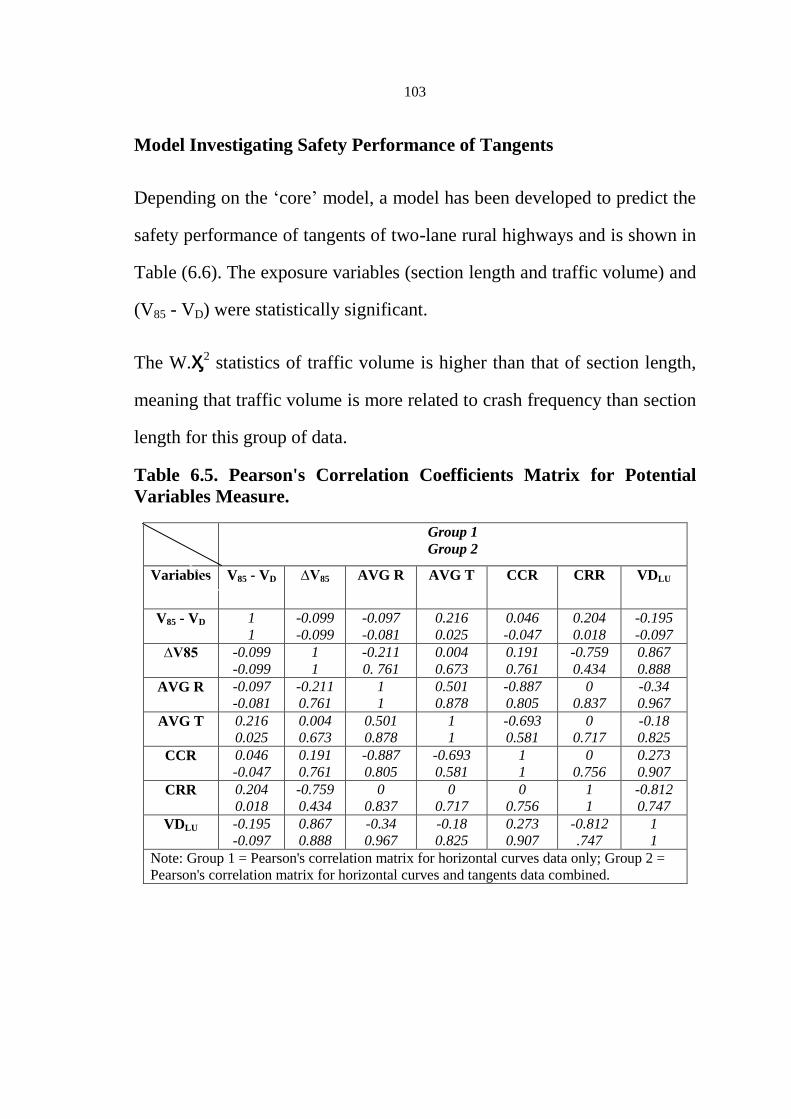
103

Model Investigating Safety Performance of Tangents

Depending on the ‘core’ model, a model has been developed to predict the

safety performance of tangents of two-lane rural highways and is shown in

Table (6.6). The exposure variables (section length and traffic volume) and

(V85 - VD) were statistically significant.

The W.Ӽ2 statistics of traffic volume is higher than that of section length,

meaning that traffic volume is more related to crash frequency than section

length for this group of data.

Table 6.5. Pearson's Correlation Coefficients Matrix for Potential

Variables Measure.

Group 1

Group 2

Variables V85 - VD ∆V85 AVG R AVG T CCR CRR VDLU

V85 - VD 1

1

-0.099

-0.099

-0.097

-0.081

0.216

0.025

0.046

-0.047

0.204

0.018

-0.195

-0.097

∆V85 -0.099

-0.099

1

1

-0.211

0. 761

0.004

0.673

0.191

0.761

-0.759

0.434

0.867

0.888

AVG R -0.097

-0.081

-0.211

0.761

1

1

0.501

0.878

-0.887

0.805

0

0.837

-0.34

0.967

AVG T 0.216

0.025

0.004

0.673

0.501

0.878

1

1

-0.693

0.581

0

0.717

-0.18

0.825

CCR 0.046

-0.047

0.191

0.761

-0.887

0.805

-0.693

0.581

1

1

0

0.756

0.273

0.907

CRR 0.204

0.018

-0.759

0.434

0

0.837

0

0.717

0

0.756

1

1

-0.812

0.747

VDLU -0.195

-0.097

0.867

0.888

-0.34

0.967

-0.18

0.825

0.273

0.907

-0.812

.747

1

1

Note: Group 1 = Pearson's correlation matrix for horizontal curves data only; Group 2 =

Pearson's correlation matrix for horizontal curves and tangents data combined.

104

Table 6.6 Model for Predicting Safety Performance of Tangent

Sections Only.

I. Crash / 5years = EXP(-1.441) EXP

(0.001( Section )) EXP(0.00014( Traffic ))

EXP(0.034 (V

85 - V

D))

Variable Parameter Significant W.Ӽ2 kD kP kM Rk2

Intercept

Section

Traffic

V85 - VD

β 1

β 2

β 3

β 4

< 0.0001

0.002

< 0.0001

0.003

12.658

9.852

29.075

8.588

0.887 0.948 0.432 0.82

Note : 1. kmax (maximum dispersion parameter of the group data equal 2.412)

2. Model statistically significant at the 95% significance level.

Models Investigating Safety Performance of Horizontal Curves

Depending on the ‘core’ model, a model has been developed to predict the

safety performance of tangents of two-lane rural highways. Three sets of

models were developed taking into consideration ∆V85, CRR , and VDLU

variables and were statistically significant in separate models. The

exposure variables (section length and traffic volume), (V85 - VD), and

∆V85 were statistically significant; the model is shown in Table (6.7).

Table 6.7 Model for Predicting Safety Performance of Horizontal

Curves Only Depending on V85 - VD and ∆V85.

II. Crash / 5years = EXP(-2.094) EXP

(0.001( Section )) EXP(0.000132( Traffic ))

EXP(0.054 (V

85 - V

D)) EXP

(0.076 ( ∆V85

))


Intercept

Section

Traffic

V85 - VD

∆V85

β 1

β 2

β 3

β 4

β 5

< 0.0001

0.001

< 0.0001

0.001

0.043

21.936

10.871

14.484

11.487

4.085

0.794 0.956 0.518 0.82

Note: 1. kmax ( maximum dispersion parameter of the group data equal 2.892)


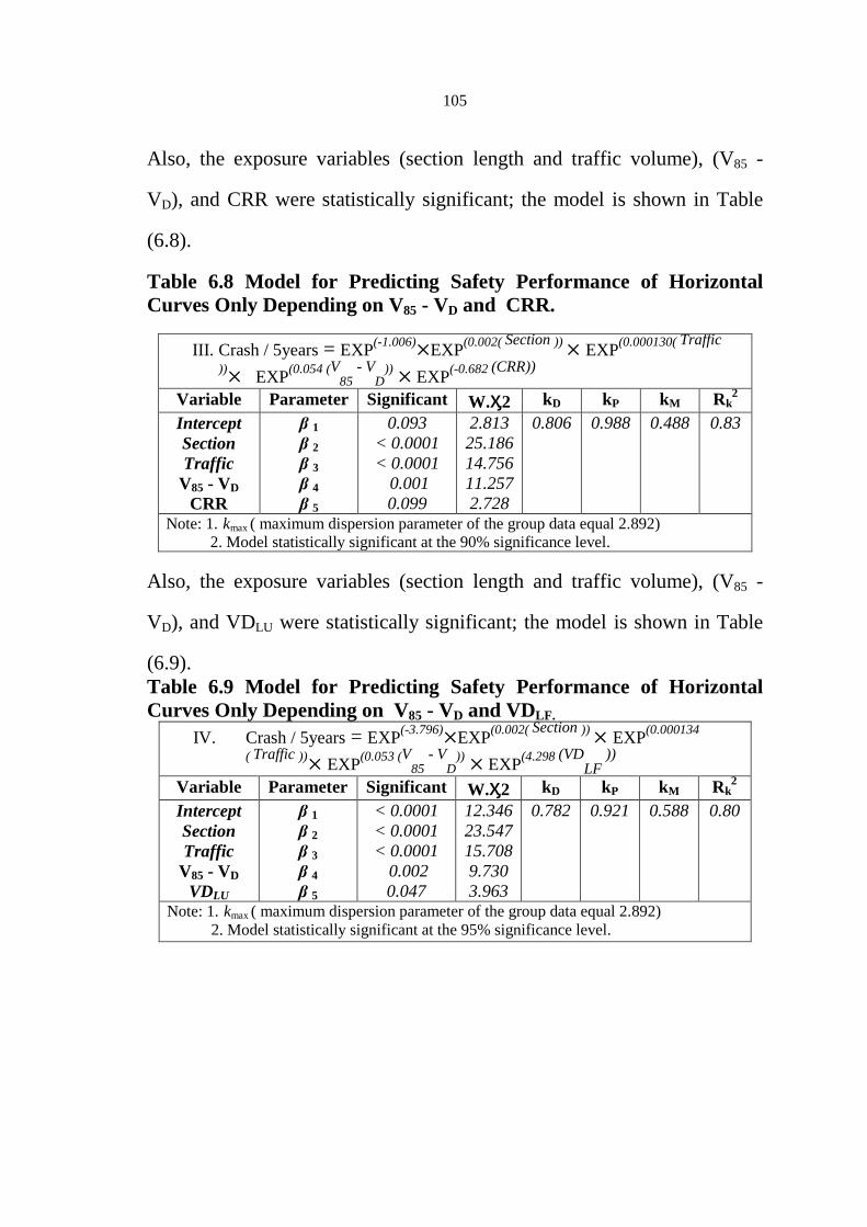
105

Also, the exposure variables (section length and traffic volume), (V85 -

VD), and CRR were statistically significant; the model is shown in Table

(6.8).


Curves Only Depending on V85 - VD and CRR.

III. Crash / 5years = EXP(-1.006) EXP

(0.002( Section )) EXP(0.000130( Traffic

)) EXP(0.054 (V

85 - V

D)) EXP

(-0.682 (CRR))


Intercept

Section

Traffic

V85 - VD

CRR

β 1

β 2

β 3

β 4

β 5

0.093

< 0.0001

< 0.0001

0.001

0.099

2.813

25.186

14.756

11.257

2.728

0.806 0.988 0.488 0.83



Also, the exposure variables (section length and traffic volume), (V85 -

VD), and VDLU were statistically significant; the model is shown in Table

(6.9).


Curves Only Depending on V85 - VD and VDLF.

IV. Crash / 5years = EXP(-3.796) EXP

(0.002( Section )) EXP(0.000134

( Traffic )) EXP(0.053 (V

85 - V

D)) EXP

(4.298 (VDLF

))


Intercept

Section

Traffic

V85 - VD

VDLU

β 1

β 2

β 3

β 4

β 5

< 0.0001

< 0.0001

< 0.0001

0.002

0.047

12.346

23.547

15.708

9.730

3.963

0.782 0.921 0.588 0.80



106

Quantitative Relationship between Geometric Design Consistency and

Road Safety.

A quantitative relationship between design consistency and crash

occurrence is an important tool in the evaluation of the impact of design

consistency on road safety (Joanne, 2002).

The models presented before (I, II, III, and IV) reveal the relationship

between significant consistency measures to road safety, whether based on

tangent data only or horizontal data only.

Therefore, one model relating as many design consistency measures as

were statistically significant to road safety to improve the model prediction

accuracy are developed depending on tangent and horizontal data

combined, which are presented in Table (6.11). Table (6.10) presents a

summary of variables used in developing model "V".

Exposure was represented in two separate terms (section and traffic) as this

approach fits the data better. Model ''V'' was developed based on both

horizontal curves and tangents data combined, and three design

consistency measures are statistically significant (V85 - VD, ∆V85, and

CRR). It should be noted that model ''V'' was applicable to both horizontal

curves and tangents with the provision of the H variable (dummy variable

as in Table 6.11).

107

Table 6.10. Summary for Variables Used in Developing Model "V".

Variable Details Sections length 90.46 km

Number of Sections 247 sections

Horizontal Curves Sections length 34.826 km

Number of Horizontal Curves

Sections

136 sections

Tangent Sections length 55.220 km

Number of Tangent Sections 111 sections

Traffic (volume) (2927 - 15160) vehicles/ day

V85 - VD ((-48.60) - (11.29)) km/hour

∆V85 (0 - 20.7) km/hour

CRR (0 - 2.02)

No. of Crashes 204 crashes in 5 years

No. of Crashes on Horizontal Curve 83 crashes in 5 years

No. of Crashes on Tangents 121 crashes in 5 years

Furthermore, from the (kD, kP, and Rk2) goodness of fit for model III, it can

be concluded that the model fits its data better than models I, II fitting their

tangent and horizontal curves data, respectively. In conclusion, because

model ''V'' is applicable to both horizontal curves and tangents and it

demonstrates a relatively better fit to its data, model ''V'' is recommended

for use in future evaluation of the impact of design consistency on road

safety.

108

Table 6.11 Model for Predicting Safety Performance of Tangent and

Horizontal Curves Combined.

V. Crash / 5years=EXP(-14.070) Section

(0.851)) Traffic(1.034) EXP

(0.037(V85

-

VD

)) EXP{H (0.052 ∆V

85 )

(0.398 (CRR ))}

Where: H = 0 for tangents or H = 1 for horizontal curves.


Intercept

Section

Traffic

V85 - VD

∆V85

CRR

β 1

β 2

β 3

β 4

β 5

β 6

< 0.0001

< 0.0001

< 0.0001

< 0.0001

0.013

0.047

71.285

56.439

32.386

14.426

6.142

3.951

0.847 1.050 0.307 0.89

Note : 1. kmax ( maximum dispersion parameter of the group data equal 2.765)


3. Units: Section= meter; Traffic= vehicles/day; V85 - VD= km/hour; ∆V85=

km/hour; and CRR= unitless.

109

Chapter Seven

Modeling Validation

To evaluate the accuracy of the West-Bank crash prediction models (CPM)

developed, a validation step was performed. The goal of this validation

step is not only to compare the accuracy of different models developed, but

also to evaluate the overall accuracy of CPMs for use on rural two-lane

highways in the West-Bank.

The necessary data for model validation were identical to the data used in

modeling development. Therefore, sources and techniques for gathering

data for modeling were used for validation.

Figure (7.1) shows the location of the highway segments for validation in

the West Bank, which are : Jerusalem to Hebron, Salfit to Za'tara, and

Bethlehem Governorate Roads. Total length of highways used for

validation is 21.4 km.

7.1 Validation of Crash Prediction Models

Validation can be thought of as a requirement to demonstrate that a model

is appropriate, meaningful, and useful for the purpose for which it is

intended. Validation exercises are often associated with assessment of the

prediction ability of a statistical model (Pedhazur and Schmelkin, 2013).

110

Figure 7.1. Location of the Highway Segments for Validation in the West Bank

111

However, it is possible for a model to predict an underlying data-

generating process adequately but fails to illuminate and explain the nature

of the underlying process. Washington et al. (2005) explained a model

validation which was broken down into two distinct aspects: internal

validity and external validity.

Internal model validity, which has been explained in chapter (5), was

concerned with the ability of the crash models to explain the underlying

phenomenon and focused on the logical defensibility, whereas external

model validity is concerned with the ability of the models to predict

crashes over time and space. The external validation tools applied are

described here.

7.1.1 The External Validation

Three sets of external validation activities were done:

1. Validation of the crash prediction algorithm. This validation activity is

used to validate the crash prediction algorithms as a whole, which is

considered to be important, provides quantitative evidence of how well it is

predicting crashes, and provides comparisons between models

performance.

2. Validation of the models against additional years of crash data for the

same sections used in the model development. This validation activity is

used to assess the models ability to forecast crashes across time and

determining the model's temporal capability and stability; meaning that the

112

effect of time or covariates that are influenced by time either is not

important or, if it is important, is included in the model in some relevant

variable expression.

3. Validation of the models against West-Bank data. This validation

activity assesses the models’ ability to forecast crashes across space;

meaning that assessing the model's ability to forecast crash on sections

whose data were not used in model development.

External validation is focused on the goodness of fit (GOF) of statistical

models. Several GOF measures were used to assess model performance in

this study. It is important to note that an objective assessment of the

predictive performance of a particular model can be made only through the

evaluation of several GOF criteria. The GOF measures used to conduct

external model validation include the following:

1. Pearson's product moment correlation coefficients between observed

and predicted crash frequencies. Pearson’s product moment correlation

coefficient, usually denoted by r, is one example of a correlation

coefficient. It is a measure of the linear association between two variables,

Y1 and Y2 that have been measured on interval or ratio scales and is given

by

r12 = ∑ ( Yi1 Ȳ1 )( Yi2 Ȳ2) [ ∑ ( Yi1 Ȳ1 ) 2 ∑ ( Yi2 Ȳ2)

2 ]

1/2 (7.1)

113

Where Ȳ is the mean of Yi observations. Theoretically, a model that

predicts observed data perfectly will produce a straight-line plot between

the observed and the predicted values, a correlation coefficient of exactly1.

2. Mean prediction bias (MPB). MPB provides a measure of the magnitude

and direction of the average model bias in comparison with validation data.

The smaller the absolute value of average prediction bias is, the better the

model does at predicting the observed data. A positive MPB indicates that

a model over-predicts crashes, on average, while a negative MPB indicates

systematic under-prediction of crashes, on average. MPB is given by

MPB = n (7.2)

Where n is the validation data sample size, and Ŷi is the fitted value of Yi.

3. Mean absolute deviation (MAD). MAD provides a measure of the

average miss-prediction of the model. It differs from MPB in that positive

and negative prediction errors do not cancel. A value close to 0 suggests

that, on average, the model predicts the observed data well. MAD is given

by

MAD = n (7.3)

Where n is the validation data sample size.

4. Mean squared prediction error (MSPE) and mean squared error (MSE).

MSPE is the sum of the squared differences between observed and

predicted crashes frequencies divided by sample size. MSPE is typically

114

used to assess the error associated with a validation or external data set and

is given by

MSPE =

2 n2 (7.4)

where n2 is the validation data sample size. MSE is the sum of the squared

differences between observed and predicted crashes frequencies divided by

the sample size minus the number of model parameters:.

MSE =

2 (n2 p) (7.5)

where n1 is the estimation data sample size and p is the number of degrees

of freedom. A comparison of MSPE and MSE reveals potential over or

under fitting of the models to the estimation data. An MSPE that is higher

than MSE may indicate that the models may have been over-fit to the

estimation data and that some of the observed relationships may have been

spurious instead of real. This finding could also indicate that important

variables were omitted from the model or the model was miss-specified.

To normalize the GOF measures to compensate for the different numbers

of years associated with different data sets, GOF measures computed on a

per-year basis. For MPB and MAD per year, MPB and MAD were divided

by the number of years. However, because MSPE and MSE are the mean

values of the squared errors, MSPE and MSE are divided by the square of

the number of years to calculate MSPE and MSE per year, which resulted

in a fair comparison of predictions based on different numbers of years.

This correction is needed because the models developed predict crashes

115

per unit of time. Because the variance in crashes is a function of the mean,

a larger time period results in both a larger number of crashes and a larger

variance in crashes, all else being equal. Computation of GOF statistics on

a per year basis normalized comparisons across models with different

numbers of years of observation.

When calculating results that were aiming for known values, the percent

error formula is useful tool for determining the precision of the

calculations. The formula is given by:

%error = |(

) | 100 (7.6)

Where ( ) was the predicted crashes frequency and ( ) was the

observed crashes frequency for n sample size (number of sites). A

percentage very close to zero means you are very close to your targeted

value, which is good.

Several goodness-of-fit (GOF) statistics to assess model fit to validation

data were employed. Assessment and comparisons between models,

however, were generally subjective. Washington et al. (2005) suggests in

the documentation to follow, the terms “serious,” “moderate,” and

“marginal” denote subjective evaluations of GOF for assessment and

comparisons between models. Serious (high) differences in GOF are

suggestive of noteworthy or significant model deficiencies. Moderate

(medium) differences in GOF suggest cases where models could be

improved, but improvements might be difficult to obtain. Marginal (low)

116

differences in GOF are thought to be negligible and are potentially

explained by random fluctuations in the observed data.

External Validity: Predictive Ability of Model Algorithm

For Model I, in terms of the GOF statistics in Table (7.1), the linear

correlation coefficient showed (0.46) value which means moderate

association between predicted and observed crashes frequency. MSE per

year2 value (1.96) indicated serious variation between predicted and

observed crash frequency. MPB per year value (0.17) indicates moderate

model over-predicting crashes, on average. MAD per year value (0.3)

indicates serious miss-prediction of the model, on average. ''%error'' value

(77%) indicates unacceptable precision of the calculations.

For Model II, in terms of the GOF statistics in Table (7.1), the linear

correlation coefficient showed (0.66) value, which means moderate

association between predicted and observed crash frequency. MSE per

year2 value (0.05) indicated marginal variation between predicted and

observed crashes frequency. MPB per year value (-0.01) indicates

marginal model under-predicting crashes, on average. MAD per year value

(0.12) indicates moderate miss-prediction of the model, on average.

''%error'' value (10%) indicates high precision of the calculations.

For Model III, in terms of the GOF statistics in Table (7.1), the linear

correlation coefficient showed (0.69) value, which means moderate to high

association between predicted and observed crash frequency. MSE per

117

year2 value (0.04) indicates marginal variation between predicted and

observed crashes frequency. MPB per year value (0) indicates model

predicts future crashes well. MAD per year value (0.09) indicates marginal

miss-prediction of the model, on average. ''%error'' value (2%) indicates

high precision of the calculations.

For Model IV, in terms of the GOF statistics in Table (7.1), the linear

correlation coefficient showed (0.64) value, which means moderate

association between predicted and observed crashes frequency. MSE per

year2 value (0.05) indicates marginal variation between predicted and

observed crash frequency. MPB per year value (0) indicates model predicts

future crashes well. MAD per year value (0.13) indicates moderate miss-

prediction of the model, on average. ''%error'' value (2%) indicates high

precision of the calculations.

For Model V, in terms of the GOF statistics in Table (7.1), the linear

correlation coefficient showed (0.77) value, which means high association

between predicted and observed crash frequency. MSE per year2 value

(0.05) indicates marginal variation between predicted and observed crash

frequency. MPB per year value (0) indicates model predicts future crashes

well. MAD per year value (0.14) indicates moderate miss-prediction of the

model, on average. ''%error'' value (1%) indicates high precision of the

calculations.

118

External Validity: Predictive Ability across Time

For Model I, a comparison of the parameter estimates is shown in Table

(7.1) for the original model and the one based on the additional years

(2003-2007) of data. In terms of the GOF statistics in Table (7.1), the

linear correlation coefficient showed a marginal decline when calculated

on the basis of the additional years data. A comparison of MSE per year2

and MSPE per year2 suggested a marginal improvement in the fit to the

later data. Similarly, the MPB per year showed marginal increases in the

lack of fit, and the MAD per year showed a marginal improvement in the

fit to the later data. ''%error'' value (95%) indicates unacceptable precision

of the calculations.

119

Table 7.1 Validation Statistics for Models I to V Total Section-Related Accidents.

Model No.

Measure I II III IV V

A B C A B C A B C A B C A B C

No. of sites 111 111 25 136 136 48 136 136 48 136 136 48 247 247 73

P. Product 0.46 0.43 0.79 0.66 0.64 0.40 0.69 .68 0.46 .64 .63 .52 0.77 .76 .73

MPB / Year 0.17 0.18 -0.03 -0.01 -0.04 -0.02 0 -0.04 -0.02 0 -0.04 -0.02 0 0.03 -0.02

MAD/ Year 0.3 0.29 .18 0.12 0.09 0.11 .12 0.09 0.11 .13 0.09 0.1 0.14 0.12 0.14

MSE/ Year2

1.96 0.05 0.04 0.05 0.05

MSPE/ Year2

1.75 0.12 0.04 0.03 0.03 0.03 0.03 0.03 0.04 0.05

%error

77% 95% 12% 10% 7% 16% 2% 17% 13% 2% 17% 17% 1% 20% 12%

NOTE: A = original data (2008 to 2012); B = additional years of data (2003 to 2007); C = West Bank data (2008 to 2012).

120

For Model II, III, IV, and V a comparison of the parameter estimates is

shown in Table (7.1) for the original model and the additional years of data.

In terms of the GOF statistics in Table (7.1), the linear correlation

coefficient showed a marginal decline when calculated on the basis of the

additional years data. A comparison of MSE per year2 and MSPE per year

2

suggests a marginal improvement in the fit to the later data. Similarly, the

MPB per year and the MAD per year showed a marginal improvement in

the fit to the later data. ''%error'' value (7%, 17%, 17%, and 20%) for Model

II, III, IV, and V respectively, indicates moderate to high precision of the

calculations based on a relative scale.

External Validity: Predictive Ability Across Space

For Model I, a comparison of the parameter estimates is shown in Table

(7.1) for the original model and the additional years data. In terms of the

GOF statistics in Table (7.1), the linear correlation coefficient showed a

serious ascent when calculated on the basis of the additional years data. A

comparison of MSE per year2 and MSPE per year

2 suggested a serious

improvement in the fit to the later data. Similarly, the MPB per year and

the MAD per year showed a serious improvement in the fit to the later data.

''%error'' value (13%) indicates moderate precision of the calculations.

For Model II, III, IV, and V a comparison of the parameter estimates is

shown in Table (7.1) for the original model and the additional years of data.

In terms of the GOF statistics in Table (7.1), the linear correlation

121

coefficient showed a marginal decline when calculated on the basis of the

additional years data. A comparison of MSE per year2 and MSPE per year

2

suggested a marginal improvement in the fit to the later data. Similarly, the

MPB per year and the MAD per year showed a marginal improvement in

the fit to the later data. ''%error'' value (17%, 14%, 18%, and 13%) for

Model II, III, IV, and V, respectively, indicates moderate precision of the

calculations.

Overall External Model Validation Results

Model I had deficiencies ranging from moderate to serious. The model

performed well across space with the associated %error, but was seriously

deficient in model algorithm validation, across time, and linear correlation

coefficient with the associated ''%error''. The reason for this is due to the

presence of significant long sections in data used to develop the model

longer than 2 km, which increases the effect of section length on the

predicted frequency of crashes while the data used to validate the model

across space had maximum section's length of 1.4 km. This problem was

overcome in developing model V, which had larger number of sections

used and more variables participate in the model development, which

reduces the effect of the section length.

Model II, III, and IV had fairly mixed validation results. The models

performed well across space, time, validation of model algorithm, and

%error with moderate linear correlation coefficient. Although Model II, III,

and IV had fairly (GOF) parameters but the weakness point was predicting

122

crash frequency for the horizontal curves only, which was compensated in

Model V, which was developed to predict crash frequency on both

horizontal curves and tangents.

Model V has good mixed validation results. The model performed well

across space, time, validation of model algorithm, and ''%error'' with high

linear correlation coefficient.

In summary, Model V is recommended for use in future evaluation of the

impact of design consistency on road safety.

123

Chapter Eight

Modeling Application

The overall purpose of investigating the relationship between geometric

design consistency and road safety is to identify inconsistent sections of an

alignment so they may be treated to improve safety. The crash prediction

models developed in this study can be used to identify inconsistent sections

and to estimate the safety benefits of improving design consistency.

Joanne (2002) suggested three applications, which make use of the. The

first application illustrates how to evaluate the safety performance of two-

lane rural highways. The second application compares the results of crash

prediction models, which explicitly consider design consistency to those

which do not. The third application presents a systematic approach to

identify inconsistent locations.

All applications use two fictitious alignments designed with intended

inconsistencies by Hassan et al. (2001). The alignments are denoted A-I

and A-II with design speed of 70 and 100 km/h, respectively. The

geometric design data are shown in Table (8.1) and the planes are shown in

Figure (8.1). All alignments are assumed to have constant lane width,

constant maximum superelevation rate, and no intersections. An average

annual daily traffic of 00511 vehicles per day is assumed for all

applications. Each alignment has eight horizontal curves (C1-C8), which

are separated by tangents and are described below:

124

Table 8.1. Horizontal Alignment Data of Two Fictitious Alignments

(Hassan et al, 2001).

Alignments A-I

(VD = 70 km/h)

Alignments A-II

(VD = 100 km/h)

Element L (m) R (m) Ls (m) L (m) R (m) Ls (m)

T1 500 — — 464.1 — —

C1 424.8 600 60 391.2 600 60

T2 300 — — 177.4 — —

C2 174.5 190 70 394.1 440 80

T3 300 — — 110.1 — —

C3 137.9 190 70 334 440 80

T4 464.4 — — 292.7 — —

C4-1 150 200 0 300 440 0

C4-2 250 400 0 500 660 0

T5 1402.4 — — 1000.2 — —

C5 508.3 450 40 709.7 600 60

T6 611.4 — — 350.3 — —

C6 891.2 1000 0 765.2 1000 0

T7 380.8 — — 374 — —

C7 130 190 70 234 440 80

T8 277.4 — — 253.9 — —

C8 120.3 200 60 77.7 200 60

T9 500 — — 502.4 — — Note: VD = design speed; L = length of circular curve or tangent; R = radius of

horizontal curve; and Ls = length of spiral curve.

Cl has a design speed of 100 km/h and C8 of 70 km/h; both allow for

the testing of the effects of transition on successive highway sections

with different design speeds.

C2 and C3 are reverse curves separated by a short tangent.

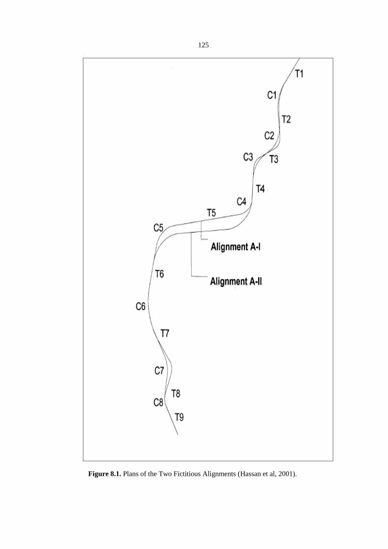
125

Figure 8.1. Plans of the Two Fictitious Alignments (Hassan et al, 2001).

126

C4 is a compound curve made up of two curves.

C5 is preceded by a long tangent T5.

C6 is a long simple curve with a radius greater than the minimum

value required.

C7 has a higher design speed than C8 on alignment A-II but not on

A-I.

In addition, the applications use model V developed in this study to

represent crash prediction models, which incorporate design consistency

measures as explanatory variables. The model has been modified slightly to

predict crash frequency for a period of one year instead of five years, as

shown in Table (8.2) below:

Table 8.2. Model (V) Crash Prediction Frequency per-Year.

Cr./years={EXP(-14.070) L

(0.851)) V(1.034) EXP

(0.037(V85

-VD

))

EXP{H (0.052 ∆V

85

0.398 (CRR )} } 5

Note : Cr./yr = predicted crash frequency per year (coll./yr); L = length of section (m), V =

average annual daily traffic (veh/day); H = dummy variable (H = 0 for tangents or H = 1 for

horizontal curves); V85-VD = the difference between operating speed and design speed;

∆V85 = speed reduction between the approach tangent and the horizontal curve (km/h); and

CRR = ratio of individual curve radius to average radius.

8.1 Model Variables Computation

The necessary data for fictitious alignments are identical to the data

necessary for modeling development and validation. Therefore, all of the

same techniques for gathering data for modeling and validation were used

as explained in section (5.3), except the 85th percentile operating speed

127

used in the difference between operating speed and design speed (V85 - VD)

variable which was computed using real time traffic speed data obtained

from Google Earth maps for modeling development and validation . The

85th percentile operating speed on tangent sections for model application

was calculated based on Al-Masaeid et al. (1995) model to predict

operating speed on tangent sections shown in Equation (8.1).

V85 = 105.47- (3792/LT) -0.27×(DC1×DC2); R2 = 0.80 (8.1)

Where:

V85 = 85th percentile operating speed (km/h);

LT = length of non-independent tangent (m); and

DC1 and DC2 = degree of successive curves for the preceding and

succeeding curves respectively/degrees/expressed in degree

per 30m.

Based on Lamm et al. (1999), tangents longer than 180m are considered

independent, tangents less than 180 m in length are considered non-

independent tangent sections. It should be noted that the model above is

applicable on independent tangent. The non-independent tangent sections

operating speed was calculated as average of operating speed of the

preceding and succeeding horizontal curves.

On the other hand, the 85th percentile operating speed on horizontal curve

sections for model application were calculated based on Kanellaidis et al.

128

(1990) model to predict operating speed on horizontal curve sections shown

in Equation (7.2).

V85 = 32.20 + 0.839VD + (2226.9 R) - (533.6 R) (8.2)

Where:

V85 = 85th percentile operating speed (km/h);

VD = design speed (km/h); and

R = radius of the curve (m).

8.2 Evaluating the Safety Performance of Two-Lane Rural

Highways

To illustrate how the crash prediction models developed in this study can

be used to evaluate the safety performance of two-lane rural highways,

model (V) has been applied on the two fictitious alignments. The results are

shown in Figure (8.2) below.

The total predicted crash frequency of alignment A-I is 20.8 crashes/year,

while that of alignment A-II is 9 crashes/year. Thus, alignment A-II is a

safer alternative than alignment A-I.

In other situations, the alignment alternative suggested may have

approximate predicted crash frequency. The role of designers is to perform

a benefit to cost analysis to determine which alternative has higher safety

benefits and reasonable economic costs.

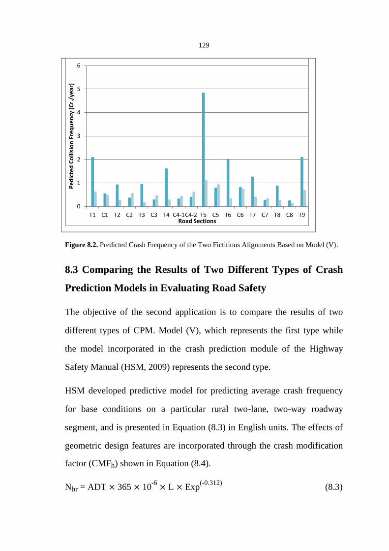
129

Figure 8.2. Predicted Crash Frequency of the Two Fictitious Alignments Based on Model (V).

8.3 Comparing the Results of Two Different Types of Crash

Prediction Models in Evaluating Road Safety

The objective of the second application is to compare the results of two

different types of CPM. Model (V), which represents the first type while

the model incorporated in the crash prediction module of the Highway

Safety Manual (HSM, 2009) represents the second type.

HSM developed predictive model for predicting average crash frequency

for base conditions on a particular rural two-lane, two-way roadway

segment, and is presented in Equation (8.3) in English units. The effects of

geometric design features are incorporated through the crash modification

factor (CMFh) shown in Equation (8.4).

Nbr = ADT 365 10-6

L Exp(-0.312)

(8.3)

0

1

2

3

4

5

6

T1 C1 T2 C2 T3 C3 T4 C4-1 C4-2 T5 C5 T6 C6 T7 C7 T8 C8 T9

Pe

dic

ted

Co

llisi

on

Fre

qu

en

cy (

Cr.

/ye

ar)

Road Sections

130

Where:

Nbr = predicted number of total crashes per year for base case (coll./yr),

ADT = average daily traffic (veh/day),

L = length of section (mi), and


The Nbr for roadway segments on rural two-lane highways were applicable

to the ADT range from zero to 17,800 vehicles per day. Application to sites

with ADTs substantially outside this range may not provide reliable results.

The base condition for horizontal alignments is a tangent roadway segment.

A CMFh has been developed to represent the manner in which crash

experience on curved alignments differ from of tangents. This CMFh

applies to total roadway segment crashes. The CMFh for horizontal

curvature is in the form of an equation taking into consideration the length,

radius, and presence or absence of spiral transitions on horizontal curves,

which yields a factor as determined in Equation (8.4) in English units

(HSM, 2009).

CMFH = (1.55Lc

0.012S) 1.55Lc (8.4)

Where:

CMFH = crash modification factor for horizontal curves;

Lc = length of horizontal curve (mi);

R = radius of horizontal curve (ft); and

131

S = 1 if spiral transition curve is present, 0 if spiral transition curve is not

present.

In applying Equation (8.4), if the radius of curvature (R) is less than 100-ft,

R is set to 100 ft. If the length of the horizontal curve (Lc) is less than 100

feet, Lc is set to 100 ft. CMFh Values are computed separately for each

horizontal curve set (a curve set consists of series of consecutive curve

elements). For each individual curve, the value Lc is the total length of the

compound curve set and the value of R is the radius of the individual curve.

If the value of CMFh is less than 1.00, the value of CMFh is set equal to

1.00.

Due to the simplicity of the fictitious alignments, predicted number of total

crashes per year on a section was determined using Equation (8.5).

Nrs = Nbr CMFh (8.5)

Where: Nrs = predicted number of total crashes per year on a section

(coll./yr),

Both models have been applied to the two fictitious alignments, the results

of which are discussed in the following sections.

8.3.1 Qualitative Analysis

The profile generated by model (V) and that by the model incorporated in

the crashes prediction module of HSM are shown in Figure (8.2) and

Figure (8.3), respectively for an average annual daily traffic of 17,500

vehicles per day. Although the general outlook of the two profiles are

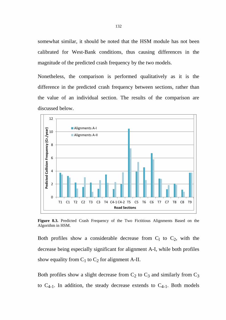
132

somewhat similar, it should be noted that the HSM module has not been

calibrated for West-Bank conditions, thus causing differences in the

magnitude of the predicted crash frequency by the two models.

Nonetheless, the comparison is performed qualitatively as it is the

difference in the predicted crash frequency between sections, rather than

the value of an individual section. The results of the comparison are

discussed below.

Figure 8.3. Predicted Crash Frequency of the Two Fictitious Alignments Based on the

Algorithm in HSM.

Both profiles show a considerable decrease from Cl to C2, with the

decrease being especially significant for alignment A-I, while both profiles

show equality from C1 to C2 for alignment A-II.

Both profiles show a slight decrease from C2 to C3 and similarly from C3

to C4-1. In addition, the steady decrease extends to C4-1. Both models

0

2

4

6

8

10

12


Pe

dic

ted

Co

llisi

on

Fre

qu

en

cy (

Cr.

/ye

ar)

Road Sections

Alignments A-I

Alignments A-II

133

predict increase from C4-1 to C4-2.From C4-2 to C5, both profiles show an

increase in crash potential. Model V profile show a considerable decrease

from C5 to C6, with the decrease being especially significant for alignment

A-II, while show equality from C5 to C6 for alignment A-I. HSM model

profile show a considerable increase from C5 to C6, with the increase being

especially significant for alignment A-I, while show slightly increase from

C5 to C6 for alignment A-II. Also, both models predict that the crash

potential at C7 decreased after C6. Finally, both models show a decrease

from C7 to C8 on A-II.

Both profiles show a considerable similarity in predicting potential crashes,

but the ability to identify inconsistent sections that may be distinguished,

which will be discussed in the following section.

8.4 A Systematic Approach to Identify Geometric Design

Inconsistencies

Although inconsistent sections may be identified by their relatively higher

crash frequency, the designer may find it difficult to decide how high is

high enough. The safety-consistency factor (SCF) proposed herein is a

practical approach to systematically identify geometrically inconsistent

sections using crash prediction models (Hassan et al, 2001). . It indicates

how much the predicted crash frequency of a section differs from that of a

tangent with identical section length and traffic volume. It is also easy to

compute. First, estimate the crash frequency of the section using model

134

(V). Then, assuming that the section is converted to a tangent, predict its

crash frequency. The ratio of the first crash frequency to the second is the

safety-consistency factor. Thus, the greater the safety-consistency factor is,

the greater the predicted crash frequency will be. A threshold value of the

safety-consistency factor should be established for a systematic

identification.

8.4.1 Establishing the Threshold Value of the Safety-Consistency

Factor

To illustrate how the threshold value of the SCF can be obtained, the two-

lane rural highway used for model development is used again. The factor is

computed for each of the 136 horizontal curves of this highway, and a

cumulative distribution of the factor is plotted in Figure (8.4). The

distribution has an average value of 1.034 and a variance of 0.147. To

establish the threshold value, the 85th

percentile value is selected (Joanne,

2002). Thus, sections of the alignment with a safety-consistency factor

greater than (1.37) can be identified as geometrically inconsistent and

should be investigated.

135

Figure 8.4. Cumulative Distribution of the Safety-Consistency Factors of Horizontal Curves of

an Existing Alignment.

8.4.2 Quantitative Analysis

To systematically identify inconsistent sections of the two fictitious

alignments, the SCF of model (V) has been computed for each section as

shown in Figure (8.5). An ADT of 17500 vehicles per day is assumed.

Using the threshold value of (1.37) established above, horizontal curves C2,

C3, C4-1, C7, and C8 of alignment A-I and C8 of alignment A-II can be

considered inconsistent. The following discusses these sections in greater

details.

0.00

20.00

40.00

60.00

80.00

100.00

120.00

.53

.5

9

.64

.6

7

.70

.7

4

.77

.8

0

.83

.8

6

.90

.9

4

.98

1

.01

1

.05

1

.11

1

.15

1

.19

1

.26

1

.31

1

.35

1

.39

1

.44

1

.66

1

.84

2

.04

2

.19

Co

mu

lati

ve F

req

ue

ncy

Safety-Consistency Factor

136

Figure 8.5. Safety-Consistency Factors Based on Model (V) of the Two Fictitious Alignments.

Model (V) predicts a considerable increase from Cl to C2, with a high

increase for alignment A-I where the design speed is reduced by 30 km/h

from Cl to C2. Thus, model can identify the inconsistency at C2 due to the

difference in its design speed to that of C1.

Model (V) predicts a slight decrease from C2 to C3 and approximately

equal from C3 to C4-1. It can be argued that the driver's level of attention

should be maintained from C2 to C3; two reverse curves with identical

curvature separated by a short tangent section. After it has been raised

when the driver travels from the flatter curve Cl to the tighter curve C2. The

crash potential on C3 should be slightly lower than that at C2 because of the

maintained level of attention. In addition, the steady equality should extend

to C4-1; the first part of the compound curve designed with a curvature

similar to that of C2 and C3 for the same reason. Model (V) accurately

0

0.2

0.4

0.6

0.8

1

1.2

1.4

1.6

1.8


Safe

ty-C

on

sist

en

cy F

acto

r

Road Sections

Alignments A-I

Alignments A-II

137

predicts a notable drop from C4-1 to C4-2 because of the larger radius of the

second part of this compound curve.

From C4-2 to C5, model (V) predicts a slight increase in crash potential.

The emergence of C5 with a moderate curvature at the end of a long

tangent may violate the driver's expectation; therefore, the crash potential at

C5 is expected to increase. Model (V) shows that C6 is the safest curve

because it is designed with a radius greater than the minimum value

required. Also, model (V) accurately predicts that the crash potential at C7

rises remarkably after C6. The driver may expect another flat curve at C7,

the element which follows C6 after a relatively short tangent. Although

both C6 and C7 share the same design speed, the selection of radius greatly

affects the consistency of the geometric design of an alignment.

Finally, model (V) shows an increase from C7 to C8 on A-II, while it shows

equality from C7 to C8 for alignment A-I. The inconsistency between C7

and C8 on A-II becomes more severe due to the design speed reduction of

30 km/h between these two elements.

To compare results for identifying inconsistent sections of the two fictitious

alignments, the safety-consistency factor of HSM module has been

computed for each section as shown in Figure (8.5). An ADT of 17500

vehicles per day is assumed. Using the threshold value of (1.3), horizontal

curve C8 of alignment A-II can be considered inconsistent.

138

Figure 8.6. Safety-Consistency Factors Based on HSM Module of the Two Fictitious

Alignments.

8.4.3 Ability to Identify Geometrically Inconsistent Sections

There were differences between model (V) and HSM module, which

distinguish their ability to identify geometrically inconsistent sections as

reflected in SCF of the sections.

The objective of SCF was to determine which models are more effective in

identifying inconsistent sections of a highway and reflecting the impact on

crash frequency than existing models (HSM module) that rely on geometric

design characteristics only.

Using the threshold value of (1.37), horizontal curves C2, C3, C4-1, C7, and

C8 of alignment A-I and C8 of alignment A-II can be considered

inconsistent. While using threshold value of (1.3) established for HSM

module, horizontal curve C8 of alignment A-II can be considered

0

0.2

0.4

0.6

0.8

1

1.2

1.4

1.6


Safe

ty-C

on

sist

en

cy F

acto

r

Road Sections

Alignments A-I

Alignments A-II

139

inconsistent. Thus, crash prediction models, which explicitly consider

design consistency can locate more inconsistencies and reflect the resulting

effect on crash potential more accurately than models which rely on

geometric design characteristics to predict crash frequency.

8.4.4 Proposed Alignments

Horizontal curves C2, C3, C4-1, and C7 of alignment A-I are more

inconsistent than the corresponding elements of alignment A-II. This may

be due to the lower design speed of A-I (70 km/h) compared to that of A-II

(100 km/h), which results in smaller radii and; therefore, lower predicted

operating speeds. Since the operating speed on tangents is almost similar,

significant speed reduction is observed from preceding tangents to these

horizontal curves of alignment A-I. Moreover, the side friction assumed is

insufficient to meet the demand on these horizontal curves of alignment A-I

due to the lower design speed. Therefore, the larger speed reduction and the

inadequate supply of side friction of alignment A-I result in higher values

of the safety-consistency factor.

Similar level of inconsistency can be observed on horizontal curve C8 of

both alignments. Since C8 is designed with a design speed of 70 km/h, high

speed reduction is observed for both alignments. The slight difference in

the value of the safety-consistency factor of the two alignments is due to

the lower side friction assumed of alignment A-II. In conclusion, the

horizontal curves, which have been identified as inconsistent should be

140

modified, if possible, to improve the overall safety performance of the

alignments.

On a separate note, although the two parts of the compound curve C4 is

designed with an identical design speed, C4-1 is classified as inconsistent

for alignment A-I while C4-2 is not. The larger radius of C4-2 allows for a

greater predicted operating speed and a lower side friction demanded;

therefore, the safety-consistency factor is lower for C4-2 than C4-l.

141

Chapter Nine

Conclusions and Recommendations

9.1 Conclusions

The concept of design consistency is one of several tools used by highway

designers to improve roadway safety. Geometric design consistency is the

conformance of a highway's geometry with driver's expectancy. When an

inconsistency exists, which violates driver's expectation; the driver may

adopt an inappropriate speed or inappropriate maneuver, leading to crashes.

Despite its importance to road safety, geometric design consistency is not

always ensured in current design practice. The most promising consistency

measures identified in previous research fall into four main categories,

namely: operating speed, vehicle stability, alignment indices, and driver

workload. This research investigates and quantifies the relationship

between design consistency and road safety in terms of expected collision

prediction frequency.

It should be noted that because of limitations in data availability, there was

a need to relay on non-Palestinian sources; Israeli sources since most study

highways are currently under Israeli control. Furthermore, speed data were

obtained from Google Maps, which comes from mobile phone users who

contribute anonymous speed information to the system. Therefore, it was

necessary to use such information although such information may be biased

towards such users and not totally random.

142

Five crash prediction models, which relate design consistency to road

safety, have been developed. These models are expected to serve as a

useful tool to help designers maximize highway safety. For a more

comprehensive evaluation of the impact of design consistency on road

safety, a model which incorporates several design consistency measures to

quantify the impact have been developed. The model shows that when

design consistency is considered, the safety performance of an alignment is

improved.

The main results and conclusions from the regression analyses are

summarized as follows:

A new approach had been used to estimate the operating speed (V85)

along two-lane rural roads using Google Earth maps. Real-time

speed traffic data were obtained from the maps. This study produced

speed prediction method using real time traffic speed data obtained

from Google Earth maps, which can be used to calculate the 85th

percentile speed along an alignment that includes both horizontal

curve sections and tangent sections.

The generalized linear regression modeling (GLM) approach is

adopted for model development. The application of both Poisson and

Negative Binomial regression techniques were investigated, and the

use of negative binomial regression was selected. The application of

negative binomial regression was found to considerably improve the

over-dispersion of all models.

143

The developed models verified that the main design consistency

measures have an important impact on safety, excluding ∆fR and

.

For ∆fR It was stated that it is likely that variables may give inverse

direction of correlation not due to a lack of a safety relationship, but

due to limitations in data accuracy obtained. For alignment index

ratio of the maximum to minimum radius (

), previous research

argued that the use of (

) is not recommended as a design

consistency measure due to its relatively low sensitivity to collision

frequency compared to other alignment indices studied.

All models adopted in this study experienced acceptable levels of

goodness of fit and over-dispersion. Furthermore, the Rk2 values of

these models were relatively high, ranging from approximately 80%

to 89%. This indicates that these models explain a large proportion

of the systematic variability in collision frequency. These results are

very promising, especially considering the complicated nature of

collision occurrence.

Validation step was performed. The goal of this validation step was

not only to compare the accuracy of different models developed, but

also to evaluate the overall accuracy of Crash Prediction Models for

use on rural two-lane highways in the West-Bank. Validation

requirement was used to demonstrate that a model is appropriate,

meaningful, and useful for the purpose for which it is intended.

A qualitative comparison has also been made to compare collision

prediction models, which explicitly consider design consistency with

144

those that rely on geometric design characteristics for predicting

collision occurrence. It has been shown that the first type is superior

as it can locate more inconsistencies and reflect the resulting effect

on collision potential more accurately than the second.

A systematic approach to identify geometrically inconsistent

locations using the safety consistency factor has been proposed.

In conclusion, because model ''V'' is applicable to both horizontal

curves and tangents and it demonstrates a relatively better fit to its

data, model ''V'' is recommended for use in future evaluation of the

impact of design consistency on road safety. The following is the

final format of the adopted model.

Model (V) Crash Prediction Frequency per-Year.

V. Crash / 5years=EXP(-4.070) Section

(0.851)) Traffic(1.034) EXP

(0.037(V85

-

VD

)) EXP{H (0.052 ∆V

85 )

(0.398 (CRR ))}

Where: H = 0 for tangents or H = 1 for horizontal curves

Note: Crash/ 5yr = predicted crash frequency per 5 year; L = length of section (m),

V = average annual daily traffic (veh/day); H = dummy variable (H = 0 for

tangents or H = 1 for horizontal curves); V85-VD = the difference between

operating speed and design speed; ∆V85 = speed reduction between the approach

tangent and the horizontal curve (km/h); and CRR = ratio of individual curve

radius to average radius.

145

9.2 Recommendations

The following recommendations are made based on the findings and

conclusions of this study:

There was a lack of information of crashes on the study highways

from Palestinian sources; therefore, it is strongly recommended that

Palestinians make the necessary arrangement to get access to such

information especially those related to crashes involving

Palestinians.

Furthermore, operating speed data were obtained from users of

Google Maps for mobile phones. Such a mobile system (3G) is not

yet available to Palestinian users, and it has to be approved by the

Israeli authority. Therefore, it is recommended that the Palestinian

Authority insists on the Israelis to give such access, as agreed with

the Israelis, because such a system carries high potential for various

traffic and transportation applications.

The prediction accuracy of crash prediction models is limited by the

quality of their independent variables. Therefore, future research

effort should be devoted to improving the prediction of these

measures.

Further research should be conducted to construct ''As-Built''

drawing for major roads in the West-Bank taking into consideration

lane width, shoulder width and type, superelevation, grades,

driveway density, and lighting because the effect of changes in cross-

146

section and the environment of highways is another source of

geometric design inconsistency.

Additional work should be conducted to obtain average annual daily

traffic (AADT) for major roads using automatic counts or in situ

counts with vehicle classifications.

Further research should be conducted to construct a database for the

crashes frequency in the West Bank. A concerted effort should be

taken from the competent authorities to gathering and documenting

these data.

Operating speed models should be developed, which reflect local

conditions for both horizontal curves and tangents. Additional

insight into the influence of speeds on tangent sections of various

lengths and grades is needed.

Alignment indices do not appear appropriate as primary measures of

design consistency because curvature change rate (CCR) only used

from the alignment indices were identified as input to the developed

models.

Additional research is desired to develop a better theoretical model

of visual demand considering design conditions (i.e., more complex

curves, intersections, signs and signals, and traffic).

The models developed in this study are limited to horizontal curves

and tangents of two-lane rural highways. More work is needed to

expand the applicability to sections, which are combined with

vertical curves. The effect of changes in cross-section is another

147

source of geometric design inconsistency, which requires further

investigation.

The models developed are expected to serve as a useful tool to help

designers maximize highway safety by identify inconsistent sections

of an alignment so they may be treated to improve safety. An

“inconsistency in design” can be described as the absence of

transition curves, the presence of reverse curves, the presence of

compound curves, the curves preceded by a lone tangents, and the

simple curves with radius less than the minimum value required

which, may led the drivers to drive in an unsafe manner. This

situation could lead to speed errors, inappropriate driving maneuvers,

and/or an undesirable level of accidents.

The model did not directly take into consideration the impact of

reverse and compound curves on road safety. Therefore, it is

recommended that future research takes this into consideration.

148

References

AASHTO. A Policy on Geometric Design of Highways and Streets.

Washington D.C., USA: American Association of State Highway and

Transportation Officials; 2011. 912 p.

Abdelwahab, W. M ., Aboul-Ela, M. T., Morrall, J. F. 1998. Geometric

Design Consistency Based on Speed Change on Horizontal Curves.

Road and Transport Research. 7 (1): 13-23.

Alexander, J., Lunenfeld, H. Driver Expectancy in Highway Design and

Traffic Operations. Washington, US: Federal Highway Administration,

Report, FHWA-TO-86-1; 1986. 39 p.

Al-Masaeid, H., Flamed, M., Aboul-Ela, M., Ghannam, A. 1995.

Consistency of Horizontal Alignment for Different Vehicle Classes.

Transportation Research Record: Journal of the Transportation

Research Board. 1500: 178-183.

Al-Masaeid, H. R., Hammory, K. K., Al-Omari, B. H. 1999. Consistency

of Horizontal Alignment Under Adverse Weather Conditions. Road and

Transport Research. 8 (3): 55-67.

Anderson, I. B., Bauer, K. M., Harwood, D. W. Fitzpatrick, K. 1999.

Relationship to Safety of Geometric Design Consistency Measures for

Rural Two-Lane Highways. Transportation Research Record. 1658:

43-51.

http://trb.metapress.com/content/120399/


149

Awatta, M. Highway Design Consistency and Safety: Individual and

Overall Evaluation Criteria. Ottawa, Canada: Carleton University; 2003.

174 p.

Babkov, V . F. Road Conditions and Traffic Safety. Moscow: MIR

Publishers; 1975. 371 p.

Barnett, J. 1936. Safe Friction Factors and Superelevation Design.

Highway Research Board, National Research Council, 16 : 69-80.

Bonneson, J. 2001. Controls for horizontal curve design.

Transportation Research Record. 1751: 82-89p.

Bonneson, A. McCoy, T. 1993. Estimation of Safety at Two-Way Stop-

Controlled Intersections on Rural Highways. Transportation Research

Record: National Research Council.1401: 83-89.

Cafiso, S., Cerni, G. 2011. A New Approach to Define Continuous Speed

Profile Models for Two-Lane Rural Roads. Transportation Research

Record: Journal of the Transportation Research Board. 2309: 157–167.

Cafiso, S., La Cava, G. Montella, A. 2007. Safety Index for Evaluation of

Two-Lane Rural Highways. Transportation Research Record: Journal

of the Transportation Research Board. 2019: 136-156.

Chen, T., Wei, L., Zhou, W. 2011. 11th International Conference of

Chinese Transportation Professionals (ICCTP): Study on the

Relationship between the Horizontal Alignment Indices and Traffic



150

Safety in Mountainous Freeway. 2011 August 14-17; Nanjing, China.

Reston, USA: American Society of Civil Engineers. 4419p.

Deacon, J. 1986. Relationship Between Accidents and Horizontal

Curvature. Appendix D, Designing Safer Roads: Practices for

Resurfacing, Restoration, and Rehabilitation. Transportation

Research Board. Special Report 214 SR 214: 256-264.

Dissanayeke, S., Ratnayake, I. 2006. Statistical Modeling of Crash

Frequency on Rural Freeways and Two-Lane Highways Using

Negative Binomial Distribution. Advance in Transportation Studies an

International Journal. B9: 81-96.

Easa, M. 2003. Distributing Superelevation to Maximize Highway

Design Consistency. Journal of Transportation Engineering. 129(2):

127-133.

Fitzpatrick, K., Collins, J. M. 2000. Speed-Profile Model for Two-Lane

Rural Highways. Transportation Research Record: Journal of the

Transportation Research Board. 1737: 42–49.

Fitzpatrick, K., Wooldridge, M . D., Tsimhoni, O., Collins, J. N., Green, P.,

Bauer, K . M. , Parma, K . D., Koppa, R., Harwood, D. W., Anderson, I.,

Krammes, R. A., and Poggioli, B. Alternative Design Consistency Rating

Methods for Two-Lane Rural Highways. Washington, US: Federal

Highway Administration, Report FHWA-RD-99-172; 2000a. 162p.

151

Fitzpatrick, K., Elefteriadou, L., Harwood, D., Collins, J., McFadden, J.,

Anderson, I. B., Krammes, R. A., Irizarry, N., Parma, K., Bauer, K., and

Passetti, K. Speed Prediction for Two-Lane Rural Highways.

Washington, US: Federal Highway Administration, Report FHWA-RD-99-

171; 2000b. 217 p.

Fitzpatrick, K., Carlson, P. J., Wooldridge, M. D., Brewer, M. A. Design

Factors that Affect Driver Speed on Suburban Arterials. US: Texas

Transportation Institute, Report FHWA/TX-00/1769-3; 2000c. 166 p.

Fitzpatrick, K., I. Anderson, K. Bauer, J. Collins, L. Elefteriadou, P. Green,

et al. August. Evaluation of Design Consistency Methods for Two Lane

Rural Highways, Executive Summary. Washington, US: Federal

Highway Administration, Report FHWA-RD-99-173: 2000d. 31p.

Garber, N., Hoel, L. Traffic and Highway Engineering. Washington,

USA: Cengage Learning; 2009. 1200 p.

Gibreel, G. M. , Easa, S. M. , El-Dimeery I. A . 2001. Prediction of

Operating Speed on Three-Dimensional Highway Alignments. Journal

of Transportation Engineering. 127(1): 21-30.

Gibreel, G. M., Easa, S. M., Hassan, Y., El-Dimeery, I. A. 1999 August.

State of the Art of Highway Geometric Design Consistency. ASCE

Journal of Transportation Engineering, 125(2): 305-313.

152

Glennon, J.C., Harwood, D.W., Free, S., Gray, C.W. 1978. Highway

Design Consistency and Systematic Design Related to Highway Safety.

Transportation Research Record. 681: 77-88.

Hassan, Y. 2004. Highway Design Consistency: Refining the State of

Knowledge and Practice. Transportation Research Record: Journal of

the Transportation Research Board. 1881: 63-71.

Hassan, Y., Sayed, T. Tabernero, V. 2001. Establishing a Practical

Approach for Design Consistency Evaluation. ASCE Journal of

Transportation Engineering. 127(4): 295-302.

Hassan, Y., Gibreel, G., Easa, S. 2000. Evaluation of Highway

Consistency and Safety: Practical Application. Journal of

Transportation Engineering. 126 (3): 193–201.

Heger, R. 1998. Driving Behavior and Driver Mental Workload As

Criteria Of Highway Geometric Design Quality. Transportation

Research Circular. E-C003: 1-10.

Hirsh, M. 1987. Probabilistic Approach to Consistency in Geometric

Design. American Society of Civil Engineers. 113(3): 268–276.

HSM. Highway Safety Manual. Washington D.C., USA: American

Associations of State Highway and Transportation Officials; 2009.

1057 p.

http://trid.trb.org/results.aspx?q=&serial=%22Transportation%20Research%20Circular%22


153

Islam, M . N., Seneviratne, P. N. 1994. Evaluation of Design Consistency

of Two-Lane Highways. Institute of Transportation Engineering

Journal. 64 (2): 28-31.

Joanne, C. and Sayed, T. 2004. Effect of Geometric Design Consistency

on Road Safety. Canadian Journal of Civil Engineering. 31(2): 218-227.

Joanne, C.W. Quantifying the Relationship Between Geometric Design

Consistency and Road Safety. British Columbia, UK: The University of

British Columbia; 2002. 103 p.

Jovanis, P. Chang, L. 1986. Modeling the Relationship of Accidents to

Miles Traveled. Transportation Research Record: National Research

Council. 1068: 42-183.

Kallberg, P. Kulmala, R. Roine, M. Accident Prediction Models for Two

Lane Roads in Finland. Espoo, Finland: Technical Research Centre of

Finland; 1987. 74 p.

Kanellaidis, G., Golias, J., Efstathiadis, S. 1990 July. Drivers Speed

Behavior on Rural Road Curves. Traffic Engineering and Control. 31

(7/8): 414–415.

Krammes, R. A., Rao, K. S., Oh, H. 1995. Highway Geometric Design

Consistency Evaluation Software. Transportation Research Record:

Journal of the Transportation Research Board. 1500: 19-24.



154

Kulakowski, B. 1991. Mathematical Model for Skid Resistance as

Function of Speed. Transportation Research Record. 1311: 26 - 32.

Kulmala, R. Safety at Rural Three and Four-Arm Junctions.

Development of Accident Prediction Models. Espoo, Finland: Technical

Research Centre of Finland; 1995. 104 p.

Lamm, R., Beck A., Ruscher T., Mailaender T., Cafiso S., La Cava G. How

to Make Two Lane Rural Roads Safer. Southampton, UK: Witpress;

2007. 144 p.

Lamm, R., Psarianos, B., Mailaender T. Highway Design and Traffic

Safety Engineering Handbook. New York, US: McGraw-Hill Companies;

1999. 1088 p.

Lamm, R., Psarianos, B., Choueri, E.M., Soilemezoglou, G. 1998. A

Practical Safety Approach to Highway Geometric Design International

Case Studies: Germany, Greece, Lebanon, and the United States.

Transportation Research Circular: Journal of the Transportation Research

Board. E-C003: 9:1-14.

Lamm, R., Psarianos, B., Guenther, A.K. 1994. The Third International

Conference on Safety and the Environment in the 21st Century:

Interrelationships Between Three Safety Criteria: Modern Highway

Geometric Design, as well as High Risk Target Locations and Groups;

1994 Nov 7-10; Tel-Aviv, Israel. Tel-Aviv: Israel Ministry of Transport.

640p.


155

Lamm, R., Choueiri, E. M., Mailaender, T. 1991. Side Friction Demand

Versus Side Friction Assumed for Curve Design on Two-Lane Rural

Highways. Transportation Research Record. 1303: 11-21.

Lamm, R., Choueiri, E. M., Hayward, J. C. 1988. Tangent as an

Independent Design Element. Transportation Research Record:

Journal of the Transportation Research Board. 1195: 123–131.

Lamm, R., Choueiri, E. M. 1987. Recommendations for Evaluating

Horizontal Design Consistency Based on Investigations in the State of

New York. Transportation Research Record: Journal of the


Lamm, R., Hayward, J., Cargin, G. 1986 .Comparison of Different

Procedures for Evaluating Speed Consistency. Transportation Research

Record, National Research Council. 1100: 10-20.

Lamm, R. 1984. Driving Dynamic Considerations: A Comparison of

German and American Friction Coefficients for Highway Design.

Transportation Research Record . 960: 13-20.

Leisch, J. E., Leisch, J. P. New Concept in Design Speed Applications, as

a Control in Achieving Consistent Highway Design. Evanston, IL, USA:

Jack E. Leisch & Associates; 1977.43 p.

Lovegrove, G., Sayed, T. 2006. Using Macro-Level Crash Prediction

Models in Road Safety Planning Applications. Transportation





156

Research Record: Journal of the Transportation Research Board. 1950:

73-82.

McFadden, J., Elefteriadou , L. 1999. Evaluating Horizontal Alignment

Design Consistency of Two-Lane Rural Highways: Development of

New Procedure. Transportation Research Record: Journal of the

Transportation Research Board. 1737: 9-17.

McFadden, J., Elefteriadou, L. 1997. Formulation and Validation of

Operating Speed-Based Models Using Bootstrapping. Transportation


97-103.

McLean, J.R. 1976. Traffic Engineering: Sessions 20-27 Proceedings of

the Eighth ARRB Conference: Vehicle Speeds on High Standard

Curves; 1976 August 23-27; Perth, Australia. Perth: Australian Road

Research Board; 8(5), Session 21. 1-8.

Messer, C.J. 1980. Methodology for Evaluating Geometric Design

Consistency. Facility Design and Operational Effects, Transportation

Research Record. 757: 7–14.

Miaou, P., Lu, A., Lum. H. 1995. Pitfalls of Using R2 to Evaluate the

Goodness of Fit of Accident Prediction Models. Transportation


6-13.







157

Misaghi, P. Hassan, Y. 2005. Modeling Operating Speed and Speed

Differential on Two-Lane Rural Roads. Journal of Transportation

Engineering.131 (6): 408–418.

Morrall, J., Talarico, R. J. 1994. Side Friction Demanded and Margins of

Safety on Horizontal Curves. Transportation Research Record:

Journal of the Transportation Research Board. 1435: 145–152.

Neter, J., Kutner, M., Nachtsheim, C., William, L. Applied Linear

Statistical Models. Illinois, USA: Irwin Professional Pub; 2004. 1408 p.

Palestinian Central Bureau of Statistics, 2011. Statistics of Transport and

Communications in the Palestinian Territories: Annual Report.

Ramallah, Palestine.

Pedhazur, J., Schmelkin, L. Measurement, Design, and Analysis: An

Integrated Approach. London, UK: Psychology Press; 2013. 840 p.

Persaud, B. Statistical Methods in Highway Safety Analysis: A

Synthesis of Highway Safety Practice. Washington, US: National

Research Council, NCHRP Synthesis 295; 2001. 75 p.

Poe, C.M., Mason, J.M. 2000. Analyzing Influence of Geometric Design

on Operating Speeds Along Low-Speed Urban Streets: Mixed Model

Approach. Transportation Research Record: Journal of the






158

Polus A., Fitzpatrick, K., Fambro, D. 2000. Predicting Operating Speeds

on Tangent Sections of Two-Lane Rural Highways. Transportation


50- 57.

Polus, A. 1980. The Relationship of Overall Geometric Characteristics

to the Safety Level of Rural Highways. Eno Transportation

Foundation, Traffic Quarterly. 34(4): 575-585.

Rabaya, R., Daifi, S., Zitawy, J. Trans West Bank Highway. Nablus,

Palestine: An-Najah National University; 2012. 123 p.

Salifu, M. Analysis Of Accident Potential at Unsignalised Urban

Junctions in Ghana. Newcastle, UK: Newcastle Upon Tyne University;

2002. 209 p.

Sawalha, Z., Sayed, T. 2006. Traffic Accident Modeling: Some

Statistical Issues. Canadian Journal of Civil Engineering. 33(9): 1115–

1123.

Sayed, T., Rodriguez, F. 1999. Accident Prediction Models for Urban

Unsignalized Intersections in British Columbia. Transportation Research

Record: 1665: 93-99.

Wambold, J. C., Henry, J. J. International PIARC Experiment to

Compare and Harmonize Texture and Skid Resistance Measurements.



159

Paris, France: PIARC Technical Committee on Surface Characteristics;

1995. 430p.

Washington, S., Persaud, B., Lyon, C., Jutaek, O. Validation of Accident

Models for Intersections. Washington, US: Federal Highway

Administration, Report, FHWA-RD-03-037; 2005. 311 p.

Wierwille, W.W. Eggemeier, F.T. 1993. Recommendations for Mental

Workload Measurement in a Test and Evaluation Environment.

Human Factors: The Journal of the Human Factors and Ergonomics

Society. 35(2): 263-281.

Wooldridge, M., Fitzpatrick, K., Harwood, D., Potts, I., Elefteriadou, L.,

Torbic, D. Geometric Design Consistency on High-Speed Rural Two-

Lane Roadways. Washington, US: American Association of State

Highway and Transportation Officials in Cooperation with the Federal

Highway Administration, NCHRP Report 502; 2003. 92 p.

Wooldridge, M . D., Fitzpatrick, K., Koppa, R, Bauer, K. 2000. Effects of

Horizontal Curvature on Driver Visual Demand. Transportation

Research Record. 1737: 71-77.

Wooldridge, M. 1994. Design Consistency and Driver Error.

Transportation Research Record. 1445: 48-155.

160

Vogt, A., Bared, J. G. 1998. Accident Models for Two-Lane Rural

Segments and Intersection. Transportation Research Record. 1635: 18-

29.

161

Appendix A:

Alignment ,Traffic Volume, and Consistency Measures Data

for Highway Segments

162

Table A.1: Alignment ,Traffic Volume, and Consistency Measures Data for Highway 55 ( Nablus to Qalqilya Road)

Stations Section Radius A2003-

2007

A2008-

2012 ADT V85

V85 -

VD ∆fR ∆V85 VDLU

AVG

T CRR

AVG

R

MR/m

R CCR

0

465.50

2 2

1516

0 84.58 -10.42

0+465.5

504.91 365.76 0 0

1516

0 79.09 -15.91 0.16

11.1

4 0.47 611.6 0.72 509.60 8.60 46.50

0+831.26

186.37

3 1

1516

0 86.54 -8.46

1+017.63

297.34 632.36 1 0

1516

0 70.29 -24.71 0.10 4.85 0.42 611.6 1.24 509.60 8.60 46.50

1+314.97

2163.89

5 1

1516

0 88.03 -6.97

3+478.86

435.70 755.35 1 0

1516

0 78.86 -16.14 0.15 4.95 0.42 611.6 1.48 509.60 8.60 46.50

3+914.56

705.95

7 1

1516

0 85.02 -9.98

4+620.50

173.31 988.84 0 0

1516

0 74.05 -20.95 0.14 2.49 0.40 611.6 1.94 509.60 8.60 46.50

4+793.81


2007

A2008-

2012 ADT V85

V85 -


AVG

T CRR

AVG

R

MR/m

R CCR

137.83

4+931.64

232.10 3688.3

163

1

5+163.74

319.45

5+483.19

94.01 199.36

5+577.20

106.32

0 0

1516

0 81.89 -13.11

5+683.52

120.07 235.80 0 0

1516

0 92.87 -2.13 0.24 9.35 0.52 611.6 0.46 509.60 8.60 46.50

5+803.59

254.98

5 0

1516

0 85.54 -9.46

6+058.57

128.45 224.00 1 0

1516

0 82.96 -12.04 0.16

10.0

2 0.53 611.6 0.44 509.60 8.60 46.50

6+187.03

300.63

0 0

1516

0 91.7 -3.3

6+487.66


2007

A2008-

2012 ADT V85

V85 -


AVG

T CRR

AVG

R

MR/m

R CCR

227.73 525.41 0 0

1516

0 87.86 -7.14 0.15 5.19 0.44 611.6 1.03 509.60 8.60 46.50

6+715.39

431.96

0 0

1516

0 104.4 9.4

7+147.35

467.12 823.91 2 0

1516

0 96.86 1.86 0.19 4.72 0.41 611.6 1.62 509.60 8.60 46.50

7+614.46

2016.88

9 0 1516 106.2 11.29

164

0 9

9+631.34

625.21 606.84 1 0

1516

0

101.4

7 6.47 0.22 7.67 0.43 611.6 1.19 509.60 8.60 46.50

10+256.56

630.79

0 0

1516

0

94.04

8 -0.952

10+887.35

605.68 480.29 1 0

1516

0 89.04 -5.96 0.19 9.50 0.44 611.6 0.94 509.60 8.60 46.50

11+493.03

135.88 878.68 0 0

1516

0 90.95 -4.05 0.22 2.60 0.41 611.6 1.72 509.60 8.60 46.50

11+628.91

605.76


2007

A2008-

2012 ADT V85

V85 -


AVG

T CRR

AVG

R

MR/m

R CCR

12+234.67

54.43 319.10

12+289.11

188.60

12+477.71

184.25 566.06

12+661.96

118.29

1354.2

2

12+780.25

118.53 829.06

12+898.78

188.89

1524.6

5

13+087.66

165

80.32 285.11

13+167.98

134.75

1857.8

0

13+302.73

690.62

5 3

1516

0 80.68 -14.32


2007

A2008-

2012 ADT V85

V85 -


AVG

T CRR

AVG

R

MR/m

R CCR

13+993.35

189.74 168.09 2 0

1516

0 75.35 -19.65 0.15

15.1

3 0.58 611.6 0.33 509.60 8.60 46.50

14+183.09

131.35

0 0

1516

0 82.17 -12.83

14+314.44

143.50 115.50 0 0

1516

0 85.5 -9.5 0.19

20.0

7 0.68 611.6 0.23 509.60 8.60 46.50

14+457.94

305.23

1 0

1516

0 87.58 -7.42

14+763.17

179.67 250.53 3 1

1516

0 81.8 -13.2 0.17 9.95 0.51 611.6 0.49 509.60 8.60 46.50

14+942.84

187.24 593.05 0 0

1516

0 85.9 -9.1 0.22 4.27 0.43 611.6 1.16 509.60 8.60 46.50

15+130.08

171.78

0 0

1516

0 82.24 -12.76

15+301.86 Fix

point

153.24 128.66 0 0 2927 79.08 -15.92 0.16 18.3 0.65 182.9 0.43 296.90 5.60 108.60

166

9

15+455.10

158.42

0 0 2927 87.32 -7.68


2007

A2008-

2012 ADT V85

V85 -


AVG

T CRR

AVG

R

MR/m

R CCR

15+613.52

61.03 258.23 0 0 2927 81.6 -13.4 0.17 7.43 0.51 182.9 0.87 296.90 5.60 108.60

15+674.55

168.91

0 0 2927 84.8 -10.2

15+843.46

163.52 305.37 1 0 2927 97.31 2.31 0.27 7.91 0.49 182.9 1.03 296.90 5.60 75.40

16+006.98

124.45

2927 86.4 -8.6

16+131.43

74.91 179.77

16+206.34

106.12

16+312.46

47.50 392.57

16+359.96

63.88 212.14

16+423.84

105.05


2007

A2008-

2012 ADT V85

V85 -


AVG

T CRR

AVG

R

MR/m

R CCR

16+528.89

69.93 182.87

16+598.82

63.47

16+662.29

188.64 328.13

16+850.94

167

218.32

1174.8

9

17+069.26

224.14

3302.5

4

17+293.40

118.45

4888.5

8

17+411.85

14.05

17+425.90

19.86 128.43

17+455.76

181.43


2007

A2008-

2012 ADT V85

V85 -


AVG

T CRR

AVG

R

MR/m

R CCR

17+637.19

32.26

1138.7

3

17+669.44

97.06 221.85

17+766.50

1416.23

2927 99.46 4.46

19+182.73

162.41 327.16 0 0 2927 98.24 3.24 0.27 7.37 0.48 182.9 1.10 296.90 5.60 108.60

19+345.14

246.99

0 0 2927 85 -10

19+592.13

65.14 108.70 0 0 2927 75 -20 0.14

17.8

3 0.70 182.9 0.37 296.90 5.60 108.60

19+657.27

65.52

0 0 2927 59.2 -35.8

168

19+722.79

76.49 466.36 0 0 2927 80 -15 0.27 4.27 0.45 182.9 1.57 296.90 5.60 108.60

19+799.29

103.40

1 0 2927 46.4 -48.6


2007

A2008-

2012 ADT V85

V85 -


AVG

T CRR

AVG

R

MR/m

R CCR

19+902.69

130.47 52.25

20+033.16

62.79

20+095.95

84.48 50.79

20+180.43

350.66

0 0 2927 88 -7

20+531.09

80.64 141.24 0 0 2927 76.8 -18.2 0.14

14.2

5 0.63 182.9 0.48 296.90 5.60 108.60

20+611.73

171.03

20+782.76

142.88 296.66

20+925.64

138.86 253.02 0 0 2927 85 -10 0.22 9.07 0.51 182.9 0.85 296.90 5.60 108.60

21+064.50

102.18

0 0 2927 80.02 -14.98


2007

A2008-

2012 ADT V85

V85 -


AVG

T CRR

AVG

R

MR/m

R CCR

21+166.68

189.94 375.79 0 0 2927 88.29 -6.71 0.24 6.77 0.46 182.9 1.27 296.90 5.60 108.60

21+356.62

117.97

0 0 2927 76.8 -18.2

21+474.59

169

249.71 598.90 0 0 2927 83.2 -11.8 0.20 4.73 0.43 182.9 2.02 296.90 5.60 108.60

21+724.30

383.31

2 0 2927 81.6 -13.4

22+077.61

140.55 285.10

22+218.15

56.91

22+275.06

50.00 322.13

22+325.05

131.73

0 0 2927 75.2 -19.8

22+456.78

186.19 180.92 0 0 2927 74.72 -20.28 0.17

13.9

6 0.57 182.9 0.61 296.90 5.60 108.60


2007

A2008-

2012 ADT V85

V85 -


AVG

T CRR

AVG

R

MR/m

R CCR

22+642.98

133.67 418.83 0 0 2927 76.54 -18.46 0.19 5.42 0.45 182.9 1.41 296.90 5.60 108.60

22+776.66

Note 1 : Section = length of alignment section (m); Radius = radius of the curve (m); AYears = Accident per 5 year; ADT = average daily traffic volume (veh/day); V85 = 85th percentile speed

(km/h); V85 - VD = difference between operating speed and design speed (km/h); ∆fR = deference between side friction supply and demand; ∆V85 = speed reduction between tangent and of curve

(km/h); VDLU = visual demand of unfamiliar drivers; AVG T = Average tangent length (m); CRR = Ratio of individual curve radius to average radius; AVG R = Average radius of curvature;

MR/mR = Maximum radius of curvature to minimum radius of curvature; CCR = Ratio of individual curve radius to average radius.

Note 2 : The sections with empty consistency measures blanks are those sections located in Urban areas which were neglected.

170

Table A.2: Alignment ,Traffic Volume, and Consistency Measures Data for Highway 60 ( Nablus to Jerusalem Road)

Stations Section Radius A2003-2007 A2008-2012 ADT V85 V85 - VD ∆fR ∆V85 VDL

U AVG T CRR AVG R MR/mR CCR

0+000.00

103.92 0 0 7518 83.20 -21.80

0+103.92

91.20 318.19 0 0 7518 89.60 -15.40 0.24 6.49 0.48 1009.60 0.63 504.60 3.20 38.60

0+195.12

776.28 324.65 0 1 7518 79.89 -25.11 0.16 16.6

0 0.48 1009.60 0.64 504.60 3.20 38.60

0+971.40

212.78 0 0 7518 86.40 -18.60

1+184.18

339.02 288.38 0 0 7518 84.72 -20.28 0.17 11.3

3 0.49 1009.60 0.57 504.60 3.20 38.60

1+523.20

648.34 0 1 7518 94.72 -10.28

2+171.53

447.28 344.02 0 0 7518 95.14 -9.86 0.23 11.0

3 0.47 1009.60 0.68 504.60 3.20 38.60

2+618.81

231.77 0 0 7518 85.66 -19.34

2+850.58



276.88 380.96 0 1 7518 93.79 -11.21 0.25 7.79 0.46 1009.60 0.75 504.60 3.20 38.60

3+127.46

180.70 0 0 7518 87.33 -17.67

3+308.16

171

278.47 742.12 0 0 7518 91.11 -13.89 0.21 4.01 0.42 1009.60 1.47 504.60 3.20 38.60

3+586.63

1148.35 0 0 7518 96.10 -8.90

4+734.99

781.91 447.22 0 1 7518 103.3

3 -1.67 0.27

12.1

1 0.45 1009.60 0.89 504.60 3.20 38.60

5+516.90

4905.41 2 1 7518 99.41 -5.59

10+422.30

472.23 625.85 1 0 7518 94.79 -10.21 0.22 6.25 0.43 1009.60 1.24 504.60 3.20 38.60

10+894.53

181.91 0 0 7518 98.92 -6.08

11+076.43

484.10 506.57 0 0 7518 94.67 -10.33 0.16 7.84 0.44 1009.60 1.00 504.60 3.20 38.60

11+560.53



1412.04 0 0 7518 115.0

7 10.07

12+972.57

500.22 583.71 3 1 7518 113.5

9 8.59 0.27 6.94 0.43 1009.60 1.16 504.60 3.20 38.60

13+472.79

441.02 0 0 7518 96.08 -8.92

13+913.82

368.67 639.23 0 0 7518 99.69 -5.31 0.23 5.34 0.42 1009.60 1.27 504.60 3.20 38.60

14+282.49

326.98 3 0 7518 103.2

2 -1.78

14+609.47

371.06 694.81 0 0 7518 106.6

3 1.63 0.27 4.93 0.42 1009.60 1.38 504.60 3.20 38.60

14+980.53

172

3094.63 6 1 7518 104.4

9 -0.51

18+075.16

147.83 892.39 0 0 7518 98.73 -6.27 0.22 2.62 0.41 1009.60 1.77 504.60 3.20 38.60

18+222.99

237.46 0 0 7518 92.26 -12.74

18+460.45



192.35 276.51 0 0 7518 93.88 -11.12 0.24 9.24 0.50 1009.60 0.55 504.60 3.20 38.60

18+652.80 fix point

222.57 0 0 10766 85.94 -19.06

18+875.37

109.83 260.49 2 0 10766 90.96 -14.04 0.20 8.27 0.51 351.30 0.53 495.60 3.70 65.50

18+985.20

86.12 0 0 10766 97.60 -7.40

19+071.32

138.00 607.21 0 0 10766 85.68 -19.32 0.17 3.77 0.43 351.30 1.23 495.60 3.70 65.50

19+209.32

94.07 437.44 0 0 10766 81.12 -23.88 0.19 4.75 0.45 351.30 0.88 495.60 3.70 65.50

19+303.39

106.96 0 0 10766 80.00 -25.00

19+410.35

187.32 307.08 0 0 10766 84.37 -20.63 0.19 8.24 0.49 351.30 0.62 495.60 3.70 65.50

19+597.67

125.85 419.96 0 1 10766 90.25 -14.75 0.24 5.32 0.45 351.30 0.85 495.60 3.70 65.50

19+723.52



246.43 0 0 10766 86.60 -18.40

19+969.95

179.15 271.52 0 0 10766 86.96 -18.04 0.20 9.18 0.50 351.30 0.55 495.60 3.70 65.50

20+149.10

173

257.14 501.34 0 0 10766 90.26 -14.74 0.23 5.72 0.44 351.30 1.01 495.60 3.70 65.50

20+406.24

254.10 571.66 0 0 10766 89.47 -15.53 0.22 4.99 0.43 351.30 1.15 495.60 3.70 65.50

20+660.34

406.10 360.63 1 0 10766 83.12 -21.88 0.18 9.96 0.47 351.30 0.73 495.60 3.70 65.50

21+066.44

177.16 0 0 10766 78.69 -26.31

21+243.60

454.91 847.03 0 0 10766 82.74 -22.26 0.18 4.52 0.41 351.30 1.71 495.60 3.70 65.50

21+698.51

180.75 663.57 1 0 10766 90.70 -14.30 0.22 3.77 0.42 351.30 1.34 495.60 3.70 65.50

21+879.26

183.33 326.90 1 0 10766 92.60 -12.40 0.22 7.68 0.48 351.30 0.66 495.60 3.70 65.50

22+062.59



487.36 0 0 10766 94.80 -10.20

22+549.95

157.62 260.68 0 0 10766 86.02 -18.98 0.18 9.16 0.51 351.30 0.53 495.60 3.70 65.50

22+707.57

237.28 616.63 0 2 10766 92.14 -12.86 0.25 4.50 0.43 351.30 1.24 495.60 3.70 65.50

22+944.85

136.62 231.08 5 0 10766 80.69 -24.31 0.16 9.89 0.52 351.30 0.47 495.60 3.70 65.50

23+081.47

260.35 0 0 10766 84.40 -20.60

23+341.82

246.87 521.83 0 0 10766 83.08 -21.92 0.17 5.40 0.44 351.30 1.05 495.60 3.70 65.50

23+588.69

233.56 0 0 10766 92.26 -12.74

23+822.25

626.17 620.17 0 1 10766 86.72 -18.28 0.16 7.52 0.43 351.30 1.25 495.60 3.70 65.50

24+448.42

419.98 0 0 10766 102.7 -2.28

174

2

24+868.40



239.00 745.90 1 0 10766 105.8

9 0.89 0.27 3.73 0.42 351.30 1.51 495.60 3.70 65.50

25+107.40

265.35 0 0 10766 90.86 -14.14

25+372.75

214.99 487.22 0 0 10766 91.31 -13.69 0.21 5.47 0.44 351.30 0.98 495.60 3.70 65.50

25+587.74

280.86 0 0 10766 94.55 -10.45

25+868.60

515.66 357.25 0 2 10766 92.17 -12.83 0.22 11.5

5 0.47 351.30 0.72 495.60 3.70 65.50

26+384.26

994.29 0 0 10766 82.60 -22.40

27+378.55

333.64 469.71 0 0 10766 93.89 -11.11 0.25 6.90 0.44 351.30 0.95 495.60 3.70 65.50

27+712.19

373.92 0 0 10766 89.12 -15.88

28+086.11

210.34 594.26 0 0 10766 90.64 -14.36 0.21 4.45 0.43 351.30 1.20 495.60 3.70 65.50

28+296.45



267.99 0 0 10766 92.99 -12.01

28+564.43

565.92 504.89 0 0 10766 92.57 -12.43 0.23 8.65 0.44 351.30 1.02 495.60 3.70 65.50

29+130.35

938.35 0 1 10766 89.97 -15.03

30+068.70

270.18 688.93 0 0 10766 96.36 -8.64 0.22 4.26 0.42 351.30 1.39 495.60 3.70 65.50

175

30+338.88

658.02 1 0 10766 100.5

2 -4.48

30+996.90

330.98 460.71 0 0 10766 90.01 -14.99 0.18 7.01 0.45 351.30 0.93 495.60 3.70 65.50

31+327.88

117.44 0 0 10766 86.22 -18.78

31+445.32

368.87 346.26 1 0 10766 83.31 -21.69 0.19 9.86 0.47 351.30 0.70 495.60 3.70 65.50

31+814.19

165.31 0 0 10766 89.14 -15.86

31+979.50



164.24 539.33 0 0 10766 83.55 -21.45 0.19 4.49 0.43 351.30 1.09 495.60 3.70 65.50

32+143.74

220.58 0 0 10766 81.88 -23.12

32+364.32

217.10 249.64 0 0 10766 81.95 -23.05 0.20 10.7

2 0.51 351.30 0.50 495.60 3.70 65.50

32+581.42

245.89 1 0 10766 76.92 -28.08

32+827.31

172.73 704.21 1 0 10766 78.48 -26.52 0.20 3.49 0.42 351.30 1.42 495.60 3.70 65.50

33+000.04

132.84 0 0 10766 76.11 -28.89

33+132.88

128.55 580.90 0 0 10766 77.38 -27.62 0.19 3.87 0.43 351.30 1.17 495.60 3.70 65.50

33+261.43

263.88 588.61 0 1 10766 77.14 -27.86 0.19 4.93 0.43 351.30 1.19 495.60 3.70 65.50

33+525.31

123.81 0 0 10766 75.20 -29.80

33+649.12

176



173.35 375.64 1 1 10766 85.86 -19.14 0.24 6.56 0.46 351.30 0.76 495.60 3.70 65.50

33+822.47

429.60 0 0 10766 77.46 -27.54

34+252.07

1687.47 791.28 2 1 10766 88.27 -16.73 0.23 12.4

0 0.41 351.30 1.60 495.60 3.70 65.50

35+939.54

591.63 1 0 10766 83.91 -21.09

36+531.17

1261.23 498.94 9 2 10766 95.85 -9.15 0.21 15.5

2 0.44 351.30 1.01 495.60 3.70 65.50

37+792.40

697.89 1 0 10766 103.5

1 -1.49

38+490.29

522.81 537.14 0 1 10766 99.80 -5.20 0.23 7.74 0.43 351.30 1.08 495.60 3.70 65.50

39+013.10

388.99 1 0 10766 82.31 -22.69

39+402.09

177

Table A.3: Alignment ,Traffic Volume, and Consistency Measures Data for Highway 60 ( Jerusalem to Hebron Road )

Stations Section Radius A2008-2012 ADT V85 V85 - VD ∆fR ∆V85 VDLU AVG T CRR AVG R MR/mR CCR

0+000.00

396.44

0 11875 92.80 -12.20

0+396.44

137.97 289.24 3 11875 91.80 -13.20 0.22 7.92 0.49 479.70 0.72 401.30 4.20 81.50

0+534.41

218.19

2 11875 86.40 -18.60

0+752.60

410.94 236.15 0 11875 102.40 -2.60 0.23 15.32 0.52 479.70 0.59 401.30 4.20 81.50

1+163.54

557.11

2 11875 108.80 3.80

1+720.65

187.90 247.64 0 11875 93.04 -11.96 0.14 10.23 0.51 479.70 0.62 401.30 4.20 81.50

1+908.55

846.71

12 11875 115.80 10.80

2+755.26

161.33 982.14 1 11875 94.40 -10.60 0.15 2.45 0.40 479.70 2.45 401.30 4.20 81.50

2+916.59


330.58 445.93 1 11875 99.20 -5.80 0.24 7.24 0.45 479.70 1.11 401.30 4.20 81.50

3+247.17

541.07

0 11875 100.80 -4.20

3+788.24

302.04 263.77 0 11875 99.20 -5.80 0.24 11.71 0.51 479.70 0.66 401.30 4.20 81.50

4+090.28

195.71 561.26 3 11875 97.60 -7.40 0.22 4.58 0.43 479.70 1.40 401.30 4.20 81.50

178

4+285.99

157.08 350.32 3 11875 103.60 -1.40 0.27 6.81 0.47 479.70 0.87 401.30 4.20 81.50

4+443.07

216.54

0 11875 99.20 -5.80

4+659.60

405.37 278.54 1 11875 96.00 -9.00 0.22 12.89 0.50 479.70 0.69 401.30 4.20 81.50

5+064.97

99.55 314.79 0 11875 94.40 -10.60 0.23 6.69 0.48 479.70 0.78 401.30 4.20 81.50

5+164.52

581.50

1 11875 88.00 -17.00

5+746.02


126.13 372.24 0 11875 88.00 -17.00 0.12 6.00 0.47 479.70 0.93 401.30 4.20 81.50

5+872.15

597.15 473.87 3 11875 93.60 -11.40 0.25 9.54 0.44 479.70 1.18 401.30 4.20 81.50

6+469.30

179

Table A.4: Alignment ,Traffic Volume, and Consistency Measures Data for Highway 505 ( Salfit to Za'tara Road )


2012 ADT V85 V85 - VD ∆fR ∆V85 VDLU

AVG

T CRR

AVG

R MR/mR CCR

0+000.00

188.04 808.84 1 3122 72.00 -23.00 0.16 3.13 0.41 594 1.18 685.40 3.00 30.50

0+188.04

181.30 775.81 0 3122 75.20 -19.80 0.11 3.22 0.41 594 1.13 685.40 3.00 30.50

0+369.34

197.00

0 3122 92.80 -2.20

0+566.34

854.86 695.98 2 3122 91.20 -3.80 0.12 8.29 0.42 594 1.02 685.40 3.00 30.50

1+421.20

1656.00

3 3122 115.20 20.20

3+077.20

285.60 899.85 2 3122 115.20 20.20 0.27 3.34 0.41 594 1.31 685.40 3.00 30.50

3+362.80

420.92

0 3122 92.33 -2.67

3+783.72

Stations Section Radius

A2008-


AVG

T CRR

AVG

R MR/mR CCR

445.99 985.42 2 3122 113.60 18.60 0.27 3.84 0.40 594 1.44 685.40 3.00 30.50

4+229.71

321.63

1 3122 104.37 9.37

4+551.34

319.06 975.80 1 3122 108.80 13.80 0.23 3.25 0.40 594 1.42 685.40 3.00 30.50

4+870.40

1396.91

3 3122 113.60 18.60

6+267.31

193.84 497.64 0 3122 96.00 1.00 0.14 5.15 0.44 594 0.73 685.40 3.00 30.50

6+461.15

1129.98

5 3122 120.00 25.00

180

7+591.13

157.86 706.26 1 3122 118.40 23.40 0.27 3.38 0.42 594 1.03 685.40 3.00 30.50

7+748.99

196.42

0 3122 100.80 5.80

7+945.41

106.81 331.26 0 3122 95.13 0.13 0.17 6.46 0.48 594 0.48 685.40 3.00 30.50

8+052.22



AVG

T CRR

AVG

R MR/mR CCR

169.53

1 3122 108.80 13.80

8+221.75

157.38 709.94 0 3122 91.20 -3.80 0.15 3.36 0.42 594 1.04 685.40 3.00 30.50

8+379.13

133.13 407.68 1 3122 92.80 -2.20 0.20 5.56 0.46 594 0.59 685.40 3.00 30.50

8+512.26

130.61 720.92 0 3122 97.60 2.60 0.25 3.13 0.42 594 1.05 685.40 3.00 30.50

8+642.87

157.77

0 3122 92.80 -2.20

8+800.64

159.46 451.56 0 3122 92.80 -2.20 0.19 5.31 0.45 594 0.66 685.40 3.00 30.50

8+960.10

293.42

1 3122 98.80 3.80

9+253.52

104.42 628.76 0 3122 88.00 -7.00 0.17 3.39 0.43 594 0.92 685.40 3.00 30.50

9+357.94

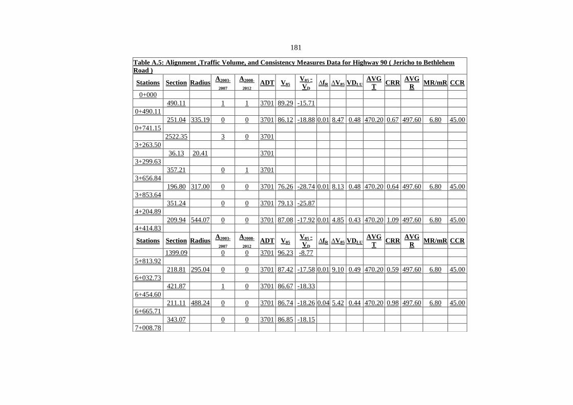
181

Table A.5: Alignment ,Traffic Volume, and Consistency Measures Data for Highway 90 ( Jericho to Bethlehem

Road )


2007

A2008-

2012 ADT V85

V85 -


AVG

T CRR

AVG

R MR/mR CCR

0+000

490.11

1 1 3701 89.29 -15.71

0+490.11

251.04 335.19 0 0 3701 86.12 -18.88 0.01 8.47 0.48 470.20 0.67 497.60 6.80 45.00

0+741.15

2522.35

3 0 3701

3+263.50

36.13 20.41

3701

3+299.63

357.21

0 1 3701

3+656.84

196.80 317.00 0 0 3701 76.26 -28.74 0.01 8.13 0.48 470.20 0.64 497.60 6.80 45.00

3+853.64

351.24

0 0 3701 79.13 -25.87

4+204.89

209.94 544.07 0 0 3701 87.08 -17.92 0.01 4.85 0.43 470.20 1.09 497.60 6.80 45.00

4+414.83


2007

A2008-

2012 ADT V85

V85 -


AVG

T CRR

AVG

R MR/mR CCR

1399.09

0 0 3701 96.23 -8.77

5+813.92

218.81 295.04 0 0 3701 87.42 -17.58 0.01 9.10 0.49 470.20 0.59 497.60 6.80 45.00

6+032.73

421.87

1 0 3701 86.67 -18.33

6+454.60

211.11 488.24 0 0 3701 86.74 -18.26 0.04 5.42 0.44 470.20 0.98 497.60 6.80 45.00

6+665.71

343.07

0 0 3701 86.85 -18.15

7+008.78

182

301.61 658.43 7 0 3701 87.73 -17.27 0.03 4.69 0.42 470.20 1.32 497.60 6.80 45.00

7+310.39

701.77

0 1 3701 91.35 -13.65

8+012.16

270.39 827.89 0 0 3701 92.18 -12.82 0.06 3.54 0.41 470.20 1.66 497.60 6.80 45.00

8+282.55

524.97

0 0 3701 88.32 -16.68

8+807.51


2007

A2008-

2012 ADT V85

V85 -


AVG

T CRR

AVG

R MR/mR CCR

416.69 627.86 0 0 3701 86.70 -18.30 0.03 5.81 0.43 470.20 1.26 497.60 6.80 45.00

9+224.20

908.98

1 0 3701 85.68 -19.32

10+133.18

264.40 590.62 0 0 3701 89.86 -15.14 0.06 4.92 0.43 470.20 1.19 497.60 6.80 45.00

10+397.57

364.59

0 0 3701 87.53 -17.47

10+762.16

200.18 684.99 0 0 3701 87.06 -17.94 0.04 3.79 0.42 470.20 1.38 497.60 6.80 45.00

10+962.34

151.27

0 0 3701 82.00 -23.00

11+113.60

262.30 749.63 0 0 3701 91.27 -13.73 0.05 3.86 0.42 470.20 1.51 497.60 6.80 45.00

11+375.91

618.56

0 0 3701 92.45 -12.55

11+994.46

225.87 769.69 0 0 3701 92.33 -12.67 0.05 3.53 0.41 470.20 1.55 497.60 6.80 45.00

12+220.33


2007

A2008-

2012 ADT V85

V85 -


AVG

T CRR

AVG

R MR/mR CCR

470.44

0 0 3701 86.40 -18.60

12+690.77

209.64 857.73 0 0 3701 90.85 -14.15 0.05 3.08 0.41 470.20 1.72 497.60 6.80 45.00

183

12+900.41

201.70

0 0 3701 90.79 -14.21

13+102.10

250.61 829.25 0 0 3701 90.51 -14.49 0.05 3.42 0.41 470.20 1.67 497.60 6.80 45.00

13+352.72

179.69 433.51 0 0 3701 89.15 -15.85 0.04 5.75 0.45 470.20 0.87 497.60 6.80 45.00

13+532.41

198.59

0 0 3701 89.27 -15.73

13+728

204.85 742.65 0 0 3701 94.54 -10.46 0.06 3.52 0.42 470.20 1.49 497.60 6.80 45.00

13+932.58

231.55

0 0 3701 93.75 -11.25

14+164.13

112.91 150.57 0 0

3701 81.37 -23.63 -

0.02 14.41 0.61 470.20 0.30 497.60 6.80 45.00


2007

A2008-

2012 ADT V85

V85 -


AVG

T CRR

AVG

R MR/mR CCR

14+277.04

211.49 542.57 0 0 3701 87.86 -17.14 0.02 4.88 0.43 470.20 1.09 497.60 6.80 45.00

14+488.53

146.61

0 0 3701 93.41 -11.59

14+635.14

184.11 349.89 0 0 3701 88.91 -16.09 0.03 7.19 0.47 470.20 0.70 497.60 6.80 45.00

14+819.25

95.19 132.20 0 0 3701 90.35 -14.65 0.05 15.76 0.64 470.20 0.27 497.60 6.80 45.00

14+914.45

189.97 802.07 0 1 3701 90.63 -14.37 0.04 3.17 0.41 470.20 1.61 497.60 6.80 45.00

15+104.42

1005.59

0 0 3701 93.70 -11.30

16+109.98

193.65 496.99 0 0 3701 96.44 -8.56 0.06 5.15 0.44 470.20 1.00 497.60 6.80 45.00

16+303.63

274.91

0 0 3701 97.47 -7.53

184

16+578.54

119.36 447.62 0 0 3701 98.10 -6.90 0.05 4.92 0.45 470.20 0.90 497.60 6.80 45.00


2007

A2008-

2012 ADT V85

V85 -


AVG

T CRR

AVG

R MR/mR CCR

16+697.89

306.32

0 0 3701 102.68 -2.32

17+004.22

102.52 321.10 1 1 3701 103.27 -1.73 0.08 6.60 0.48 470.20 0.65 497.60 6.80 45.00

17+106.74

273.94

0 0 3701 93.92 -11.08

17+380.67

245.29 366.61 0 0 3701 93.92 -11.08 0.03 7.67 0.47 470.20 0.74 497.60 6.80 45.00

17+625.97

286.93

0 0 3701 99.60 -5.40

17+912.89

218.07 320.27 1 0 3701 104.67 -0.33 0.08 8.37 0.48 470.20 0.64 497.60 6.80 45.00

18+130.96

1365.78

0 0 3701 103.88 -1.12

19+496.74

257.39 504.33 0 0 3701 90.32 -14.68 0.00 5.69 0.44 470.20 1.01 497.60 6.80 45.00

19+754.13

804.75

1 0 3701 86.28 -18.72


2007

A2008-

2012 ADT V85

V85 -


AVG

T CRR

AVG

R MR/mR CCR

20+558.88

231.14 456.34 0 0 3701 90.60 -14.40 0.05 6.01 0.45 470.20 0.92 497.60 6.80 45.00

20+790.02

321.11

1 0 3701 90.45 -14.55

21+111.13

227.11 562.80 3 0 3701 90.83 -14.17 0.04 4.84 0.43 470.20 1.13 497.60 6.80 45.00

21+338.24

162.46

0 0 3701 93.42 -11.58

21+500.70

185

207.69 603.28 0 0 3701 90.98 -14.02 0.03 4.36 0.43 470.20 1.21 497.60 6.80 45.00

21+708.38

884.63

0 0 3701 96.93 -8.07

22+593.01

136.70 469.95 0 0 3701 90.83 -14.17 0.03 4.86 0.44 470.20 0.94 497.60 6.80 45.00

22+729.71

884.62

0 0 3701 96.83 -8.17

23+576.66

189.45 756.24 0 0 3701 97.21 -7.79 0.05 3.36 0.42 470.20 1.52 497.60 6.80 45.00


2007

A2008-

2012 ADT V85

V85 -


AVG

T CRR

AVG

R MR/mR CCR

23+766.11

97.04

0 0 3701 100.00 -5.00

23+863.15

176.44 610.93 0 0 3701 91.36 -13.64 0.02 4.06 0.43 470.20 1.23 497.60 6.80 45.00

24+039.59

201.06

0 0 3701 92.50 -12.50

24+240.65

89.91 685.96 0 0 3701 106.36 1.36 0.11 3.00 0.42 470.20 1.38 497.60 6.80 45.00

24+330.56

212.20 640.74 0 0 3701 92.17 -12.83 0.00 4.14 0.42 470.20 1.29 497.60 6.80 45.00

24+542.75

409.12

0 0 3701 87.00 -18.00

24+951.88

210.23 341.93 0 0 3701 85.92 -19.08 0.03 7.73 0.47 470.20 0.69 497.60 6.80 45.00

25+162.10

219.72

0 0 3701 84.60 -20.40

25+381.82

126.16 298.73 0 0 3701 94.08 -10.92 0.08 7.48 0.49 470.20 0.60 497.60 6.80 45.00


2007

A2008-

2012 ADT V85

V85 -


AVG

T CRR

AVG

R MR/mR CCR

25+507.98

157.54

0 0 3701 88.26 -16.74

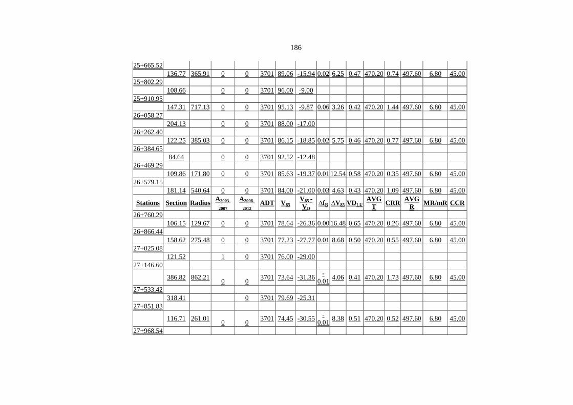
186

25+665.52

136.77 365.91 0 0 3701 89.06 -15.94 0.02 6.25 0.47 470.20 0.74 497.60 6.80 45.00

25+802.29

108.66

0 0 3701 96.00 -9.00

25+910.95

147.31 717.13 0 0 3701 95.13 -9.87 0.06 3.26 0.42 470.20 1.44 497.60 6.80 45.00

26+058.27

204.13

0 0 3701 88.00 -17.00

26+262.40

122.25 385.03 0 0 3701 86.15 -18.85 0.02 5.75 0.46 470.20 0.77 497.60 6.80 45.00

26+384.65

84.64

0 0 3701 92.52 -12.48

26+469.29

109.86 171.80 0 0 3701 85.63 -19.37 0.01 12.54 0.58 470.20 0.35 497.60 6.80 45.00

26+579.15

181.14 540.64 0 0 3701 84.00 -21.00 0.03 4.63 0.43 470.20 1.09 497.60 6.80 45.00


2007

A2008-

2012 ADT V85

V85 -


AVG

T CRR

AVG

R MR/mR CCR

26+760.29

106.15 129.67 0 0 3701 78.64 -26.36 0.00 16.48 0.65 470.20 0.26 497.60 6.80 45.00

26+866.44

158.62 275.48 0 0 3701 77.23 -27.77 0.01 8.68 0.50 470.20 0.55 497.60 6.80 45.00

27+025.08

121.52

1 0 3701 76.00 -29.00

27+146.60

386.82 862.21 0 0

3701 73.64 -31.36 -

0.01 4.06 0.41 470.20 1.73 497.60 6.80 45.00

27+533.42

318.41

0 3701 79.69 -25.31

27+851.83

116.71 261.01 0 0

3701 74.45 -30.55 -

0.01 8.38 0.51 470.20 0.52 497.60 6.80 45.00

27+968.54

187

171.46 876.70 0 0

3701 69.76 -35.24 -

0.01 2.80 0.41 470.20 1.76 497.60 6.80 45.00

28+140

170.46 192.90 0 0 3701 73.48 -31.52 0.02 12.70 0.56 470.20 0.39 497.60 6.80 45.00


2007

A2008-

2012 ADT V85

V85 -


AVG

T CRR

AVG

R MR/mR CCR

28+310.47

84.22 202.45 0 0

3701 66.80 -38.20 -

0.06 10.03 0.55 470.20 0.41 497.60 6.80 45.00

28+394.69

156.38

0 0 3701 82.02 -22.98

28+551.07

183.90 567.43 0 0

3701 58.00 -47.00 -

0.13 4.43 0.43 470.20 1.14 497.60 6.80 45.00

28+734.97

369.50

0 0 3701 85.96 -19.04

29+104.47

189.83 572.60 0 0 3701 81.90 -23.10 0.00 4.44 0.43 470.20 1.15 497.60 6.80 45.00

29+294.30

272.49

0 0 3701 89.12 -15.88

29+566.80

317.75 314.26 0 0

3701 86.16 -18.84 -

0.02 10.07 0.48 470.20 0.63 497.60 6.80 45.00

29+884.55

849.61

1 0 3701 102.42 -2.58


2007

A2008-

2012 ADT V85

V85 -


AVG

T CRR

AVG

R MR/mR CCR

30+734.16

274.17 810.37 0 0 3701 90.90 -14.10 0.01 3.64 0.41 470.20 1.63 497.60 6.80 45.00

31+008.33

1285.76

0 0 3701 96.44 -8.56

32+294.09

212.76 261.88 0 0 3701 85.51 -19.49 0.00 10.14 0.51 470.20 0.53 497.60 6.80 45.00

188

32+506.85

202.31

0 0 3701 85.89 -19.11

32+709.16

157.53 335.77 0 0 3701 82.13 -22.87 0.02 7.11 0.48 470.20 0.67 497.60 6.80 45.00

32+866.69

226.54 455.63 0 0 3701 82.42 -22.58 0.03 5.97 0.45 470.20 0.92 497.60 6.80 45.00

33+093.22

133.90

0 0 3701 79.00 -26.00

33+227.12

94.42 339.67 0 0 3701 77.90 -27.10 0.00 6.12 0.47 470.20 0.68 497.60 6.80 45.00

33+321.55

252.70

0 0 3701 84.70 -20.30


2007

A2008-

2012 ADT V85

V85 -


AVG

T CRR

AVG

R MR/mR CCR

33+574.25

116.50 425.74 0 0 3701 84.82 -20.18 0.02 5.14 0.45 470.20 0.86 497.60 6.80 45.00

33+690.75

150.47

0 0 3701 88.42 -16.58

33+841.22

178.39 864.98 0 0 3701 88.82 -16.18 0.05 2.88 0.41 470.20 1.74 497.60 6.80 45.00

34+019.60

145.64 311.33 0 0 3701 82.13 -22.87 0.01 7.48 0.48 470.20 0.63 497.60 6.80 45.00

189

Table A.6.: Alignment ,Traffic Volume, and Consistency Measures Data for Highway 90 ( Bethlehem Governorate

Road)



AVG

T CRR

AVG

R MR/mR CCR

0+000.00

101.45 236.19 0 3701 72.00 -33.00 0.03 8.95 0.52 280.60 0.59 400.00 6.20 102.40

0+101.45

173.27 433.10 1 3701 67.00 -38.00 -

0.02 5.69 0.45 280.60 1.08 400.00 6.20 102.40

0+274.72

105.00 276.79 0 3701 61.32 -43.68 -

0.04 7.70 0.50 280.60 0.69 400.00 6.20 102.40

0+379.72

85.65 155.53 0 3701 57.07 -47.93 -

0.04 13.10 0.60 280.60 0.39 400.00 6.20 102.40

0+465.37

171.73 0 3701 60.00 -45.00

0+637.10

77.11 370.56 0 3701 53.44 -51.56 -

0.06 5.39 0.47 280.60 0.93 400.00 6.20 102.40

0+714.21

59.65 357.95 0 3701 49.60 -55.40 -

0.08 5.34 0.47 280.60 0.89 400.00 6.20 102.40

0+773.86

190.43 498.48 0 3701 60.00 -45.00 -

0.04 5.11 0.44 280.60 1.25 400.00 6.20 102.40

0+964.29



AVG

T CRR

AVG

R MR/mR CCR

139.48 0 3701 66.00 -39.00

1+103.77

310.64 937.79 0 3701 68.00 -37.00 0.00 3.34 0.41 280.60 2.34 400.00 6.20 102.40

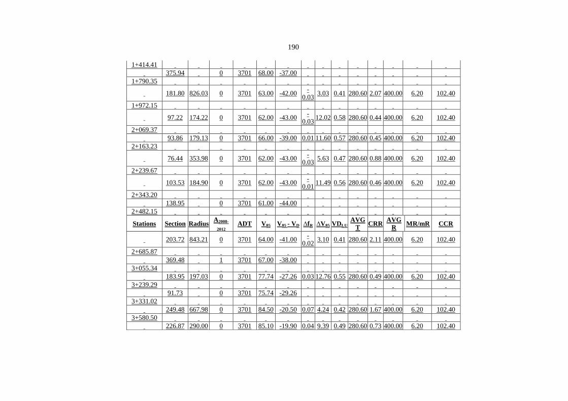
190

1+414.41

375.94 0 3701 68.00 -37.00

1+790.35

181.80 826.03 0 3701 63.00 -42.00 -

0.03 3.03 0.41 280.60 2.07 400.00 6.20 102.40

1+972.15

97.22 174.22 0 3701 62.00 -43.00 -

0.03 12.02 0.58 280.60 0.44 400.00 6.20 102.40

2+069.37

93.86 179.13 0 3701 66.00 -39.00 0.01 11.60 0.57 280.60 0.45 400.00 6.20 102.40

2+163.23

76.44 353.98 0 3701 62.00 -43.00 -

0.03 5.63 0.47 280.60 0.88 400.00 6.20 102.40

2+239.67

103.53 184.90 0 3701 62.00 -43.00 -

0.01 11.49 0.56 280.60 0.46 400.00 6.20 102.40

2+343.20

138.95 0 3701 61.00 -44.00

2+482.15



AVG

T CRR

AVG

R MR/mR CCR

203.72 843.21 0 3701 64.00 -41.00 -

0.02 3.10 0.41 280.60 2.11 400.00 6.20 102.40

2+685.87

369.48 1 3701 67.00 -38.00

3+055.34

183.95 197.03 0 3701 77.74 -27.26 0.03 12.76 0.55 280.60 0.49 400.00 6.20 102.40

3+239.29

91.73 0 3701 75.74 -29.26

3+331.02

249.48 667.98 0 3701 84.50 -20.50 0.07 4.24 0.42 280.60 1.67 400.00 6.20 102.40

3+580.50

226.87 290.00 0 3701 85.10 -19.90 0.04 9.39 0.49 280.60 0.73 400.00 6.20 102.40

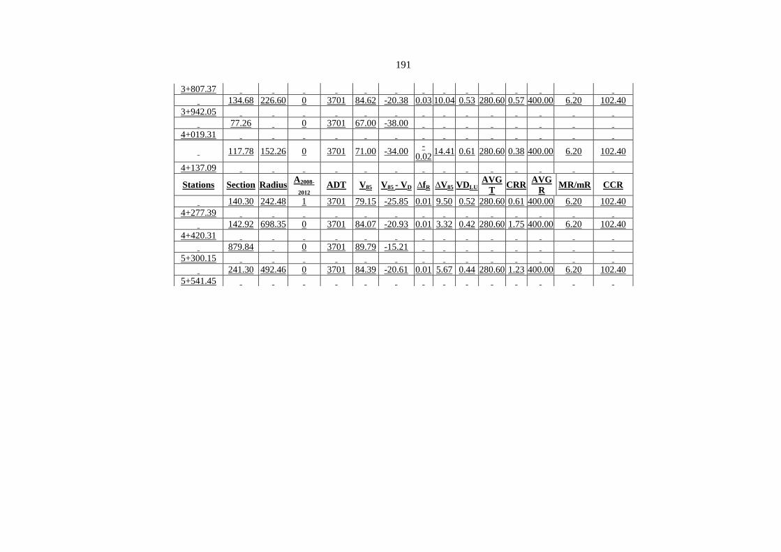
191

3+807.37

134.68 226.60 0 3701 84.62 -20.38 0.03 10.04 0.53 280.60 0.57 400.00 6.20 102.40

3+942.05

77.26 0 3701 67.00 -38.00

4+019.31

117.78 152.26 0 3701 71.00 -34.00 -

0.02 14.41 0.61 280.60 0.38 400.00 6.20 102.40

4+137.09



AVG

T CRR

AVG

R MR/mR CCR

140.30 242.48 1 3701 79.15 -25.85 0.01 9.50 0.52 280.60 0.61 400.00 6.20 102.40

4+277.39

142.92 698.35 0 3701 84.07 -20.93 0.01 3.32 0.42 280.60 1.75 400.00 6.20 102.40

4+420.31

879.84 0 3701 89.79 -15.21

5+300.15

241.30 492.46 0 3701 84.39 -20.61 0.01 5.67 0.44 280.60 1.23 400.00 6.20 102.40

5+541.45

192

Appendix B

Crash Data for Highway Segments

193

Table B.1: Crash Data for Highway 55 ( Nablus to Qalqilya Road)

Year Month Day of the Week Day / Night Crash Severity Type of Crash Casualties Vehicle X Y

2003 July Wednesday Day Slight Over-Turn Crash 1 1 166751 180307

2003 July Tuesday Day Slight Front-Side Crash 1 2 149804 176643

2003 July Wednesday Day Slight Head-On Crash 4 3 147395 175581

2003 July Tuesday Day Serious Head-On Crash 4 2 152127 176770

2003 July Sunday Day Slight Ran-Off Crash 1 1 160073 176223

2003 July Thursday Day Serious Rear-End Crash 5 2 148939 176159

2003 July Sunday Night Slight Skidding Crash 1 1 148021 175803

2003 March Sunday Day Slight Front-Side Crash 2 2 151758 176922

2003 April Tuesday Night Slight Over-Turn Crash 1 1 150691 177038

2003 December Thursday Night Slight Front-Side Crash 1 2 159129 175935

2003 December Wednesday Night Slight Front-Side Crash 5 2 148939 176160

2003 January Sunday Night Slight Over-Turn Crash 1 1 160806 176737

2003 January Tuesday Night Slight Front-Side Crash 2 3 152602 176665

2003 October Thursday Night Slight Rear-End Crash 4 2 162449 176757

2003 October Wednesday Night Slight Ran-Off Crash 4 1 165922 180092

2003 November Monday Day Slight Ran-Off Crash 1 2 154037 176424


2003 June Sunday Day Fatal Ran-Off Crash 1 2 165922 180093

2003 June Monday Day Slight Rear-End Crash 8 2 163239 177600

2003 June Wednesday Day Serious Over-Turn Crash 2 1 152602 176665

2003 May Saturday Night Slight Over-Turn Crash 1 1 152791 176606

2003 January Monday Day Slight Rear-End Crash 1 2 155017 176577

194

2003 September Sunday Night Slight Front-Side Crash 2 2 149380 176387

2003 November Wednesday Night Slight Front-Side Crash 1 2 148187 175911

2003 December Sunday Night Serious Rear-End Crash 2 2 149804 176646

2003 December Tuesday Night Fatal Front-Side Crash 1 2 159608 176049

2003 September Tuesday Day Slight Front-Side Crash 1 2 148305 175952

2004 May Saturday Day Serious Front-Side Crash 4 2 148305 175952

2004 May Thursday Day Slight Front-Side Crash 2 2 152127 176772

2004 May Sunday Day Slight Ran-Off Crash 2 1 157541 175909

2004 January Sunday Day Slight Front-Side Crash 1 2 154528 176496

2004 January Thursday Night Slight Head-On Crash 2 2 150692 177036

2004 October Monday Day Serious Head-On Crash 2 3 152126 176772

2004 July Sunday Day Slight Rear-End Crash 1 2 148021 175804

2004 August Monday Night Fatal Front-Side Crash 2 2 151665 176957


2004 August Tuesday Day Slight Front-Side Crash 3 2 154528 176496

2004 August Tuesday Day Slight Rear-End Crash 7 3 154528 176496

2004 April Saturday Night Slight Over-Turn Crash 2 1 152602 176664

2004 January Thursday Night Slight Front-Side Crash 2 2 147194 175579

2004 February Friday Day Slight Front-Side Crash 2 2 149803 176645

2004 February Saturday Night Slight Front-Side Crash 4 3 166783 180300

2004 December Saturday Night Serious Rear-End Crash 8 2 155955 176746

2004 December Tuesday Day Serious Rear-End Crash 6 2 149804 176644

2004 June Tuesday Day Slight Front-Side Crash 2 3 160074 176224

2004 June Monday Day Slight Rear-End Crash 2 3 147492 175581


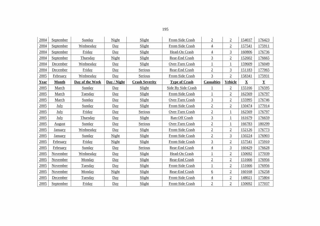
195


2004 September Wednesday Day Slight Front-Side Crash 4 2 157541 175911

2004 September Friday Day Slight Head-On Crash 4 3 160806 176736

2004 September Thursday Night Slight Rear-End Crash 3 2 152602 176665

2004 December Wednesday Day Slight Over-Turn Crash 1 1 159609 176049

2004 December Friday Day Serious Rear-End Crash 2 3 151183 177065

2005 February Wednesday Day Serious Front-Side Crash 3 2 158341 175931


2005 March Sunday Day Slight Side By Side Crash 1 2 155166 176595

2005 March Tuesday Day Slight Front-Side Crash 1 2 162569 176797

2005 March Sunday Day Slight Over-Turn Crash 3 2 155995 176746

2005 July Sunday Day Slight Front-Side Crash 2 2 150474 177014

2005 July Friday Day Serious Over-Turn Crash 2 1 162569 176797

2005 July Thursday Day Slight Ran-Off Crash 3 1 161679 176659

2005 August Sunday Day Serious Over-Turn Crash 2 1 166783 180299

2005 January Wednesday Day Slight Front-Side Crash 2 2 152126 176773

2005 January Sunday Night Slight Front-Side Crash 2 3 150224 176903

2005 February Friday Night Slight Front-Side Crash 3 2 157541 175910

2005 February Sunday Day Serious Rear-End Crash 4 3 160429 176628

2005 November Wednesday Day Slight Head-On Crash 1 2 150692 177039

2005 November Monday Day Slight Rear-End Crash 2 2 151666 176956

2005 November Tuesday Day Slight Front-Side Crash 1 2 151666 176956

2005 November Monday Night Slight Rear-End Crash 6 2 160168 176258

2005 December Tuesday Day Slight Front-Side Crash 4 2 148021 175804

2005 September Friday Day Slight Front-Side Crash 2 2 150692 177037

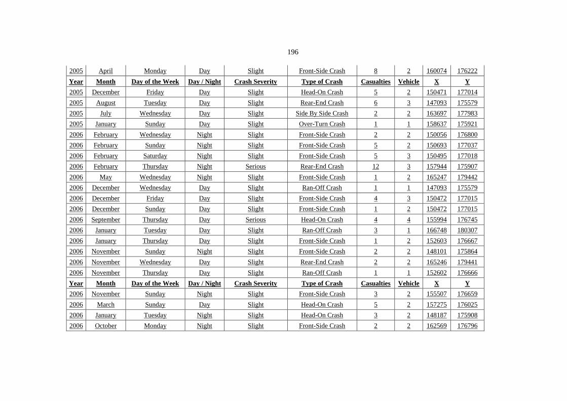
196

2005 April Monday Day Slight Front-Side Crash 8 2 160074 176222


2005 December Friday Day Slight Head-On Crash 5 2 150471 177014


2005 July Wednesday Day Slight Side By Side Crash 2 2 163697 177983

2005 January Sunday Day Slight Over-Turn Crash 1 1 158637 175921

2006 February Wednesday Night Slight Front-Side Crash 2 2 150056 176800

2006 February Sunday Night Slight Front-Side Crash 5 2 150693 177037


2006 February Thursday Night Serious Rear-End Crash 12 3 157944 175907

2006 May Wednesday Night Slight Front-Side Crash 1 2 165247 179442

2006 December Wednesday Day Slight Ran-Off Crash 1 1 147093 175579

2006 December Friday Day Slight Front-Side Crash 4 3 150472 177015

2006 December Sunday Day Slight Front-Side Crash 1 2 150472 177015

2006 September Thursday Day Serious Head-On Crash 4 4 155994 176745

2006 January Tuesday Day Slight Ran-Off Crash 3 1 166748 180307

2006 January Thursday Day Slight Front-Side Crash 1 2 152603 176667

2006 November Sunday Night Slight Front-Side Crash 2 2 148101 175864

2006 November Wednesday Day Slight Rear-End Crash 2 2 165246 179441

2006 November Thursday Day Slight Ran-Off Crash 1 1 152602 176666



2006 March Sunday Day Slight Head-On Crash 5 2 157275 176025

2006 January Tuesday Night Slight Head-On Crash 3 2 148187 175908

2006 October Monday Night Slight Front-Side Crash 2 2 162569 176796

197

2006 October Saturday Night Fatal Front-Side Crash 5 2 160708 176725

2006 October Friday Day Serious Over-Turn Crash 1 1 156574 176721

2006 October Wednesday Day Serious Side By Side Crash 8 2 166748 180306

2006 October Friday Night Slight Head-On Crash 3 2 150472 177014

2006 July Tuesday Day Fatal Over-Turn Crash 2 2 166748 180306

2006 July Thursday Day Slight Rear-End Crash 6 3 152125 176772

2006 August Tuesday Night Slight Head-On Crash 4 3 148101 175864

2006 August Monday Day Slight Front-Side Crash 3 2 150471 177015


2006 June Monday Day Serious Front-Side Crash 7 2 150691 177037

2007 November Saturday Night Serious Head-On Crash 2 2 147092 175579

2007 November Thursday Night Slight Over-Turn Crash 3 1 160168 176255

2007 March Wednesday Night Slight Front-Side Crash 2 2 150471 177015

2007 April Thursday Day Slight Side By Side Crash 1 2 164760 178791


2007 May Wednesday Day Slight Head-On Crash 2 3 164853 178815

2007 June Tuesday Night Slight Front-Side Crash 4 3 148469 176001

2007 June Thursday Day Slight Front-Side Crash 2 2 162570 176796

2007 June Wednesday Day Slight Front-Side Crash 2 2 150471 177016


2007 August Monday Day Slight Head-On Crash 1 3 159129 175934

2007 January Monday Day Slight Front-Side Crash 2 2 157542 175909

2007 February Wednesday Day Slight Front-Side Crash 1 2 162624 176840

2007 October Tuesday Night Fatal Over-Turn Crash 2 1 166088 180269

2007 November Thursday Night Fatal Head-On Crash 2 2 154528 176494

198

2007 December Thursday Day Slight Front-Side Crash 2 2 148305 175951

2007 February Saturday Night Slight Rear-End Crash 7 3 149887 176696

2007 March Thursday Night Slight Head-On Crash 2 2 152127 176773

2008 June Sunday Day Serious Head-On Crash 6 2 149022 176196

2008 June Sunday Day Slight Rear-End Crash 1 2 157136 176166

2008 June Wednesday Night Slight Side By Side Crash 1 2 153560 176547

2008 June Thursday Night Slight Side By Side Crash 3 2 155155 176593

2008 June Thursday Night Slight Rear-End Crash 5 3 155017 176577


2008 July Friday Day Slight Over-Turn Crash 1 1 165247 179440

2008 July Monday Day Slight Front-Side Crash 5 3 160167 176256

2008 July Wednesday Day Slight Front-Side Crash 2 2 160616 176691

2008 April Thursday Day Slight Rear-End Crash 4 3 162570 176797

2008 April Tuesday Day Slight Front-Side Crash 2 2 163238 177600

2008 January Wednesday Day Slight Side By Side Crash 2 2 148023 175803

2008 January Saturday Night Slight Rear-End Crash 6 2 152695 176628

2008 February Monday Day Slight Rear-End Crash 1 2 148023 175803


2008 February Monday Day Slight Over-Turn Crash 1 1 166748 180307

2008 January Friday Night Slight Side By Side Crash 5 2 165987 180166

2008 January Saturday Day Slight Front-Side Crash 4 2 152320 176745

2008 November Friday Night Serious Head-On Crash 7 2 152693 176630


2008 March Friday Night Slight Front-Side Crash 2 2 152512 176702


199

2008 November Sunday Day Slight Head-On Crash 4 2 156388 176799

2008 November Wednesday Night Slight Head-On Crash 3 2 149804 176644


2008 December Monday Day Slight Front-Side Crash 2 2 150471 177014

2008 July Saturday Day Slight Over-Turn Crash 1 1 158141 175918

2008 July Saturday Night Slight Head-On Crash 6 2 166747 180308


2008 May Thursday Night Slight Rear-End Crash 1 2 158042 175913

2008 May Wednesday Day Serious Head-On Crash 2 2 149466 176435


2008 June Thursday Day Serious Front-Side Crash 3 3 155801 176710

2008 August Tuesday Night Slight Over-Turn Crash 2 1 166747 180308

2008 August Tuesday Night Slight Front-Side Crash 2 2 150471 177014

2008 September Saturday Day Slight Front-Side Crash 2 2 151182 177064



2009 January Wednesday Night Slight Front-Side Crash 1 2 149804 176642

2009 January Thursday Night Slight Rear-End Crash 7 2 165659 179675






2009 December Tuesday Night Slight Rear-End Crash 1 2 148021 175803

2009 December Tuesday Night Slight Head-On Crash 3 3 165246 179440

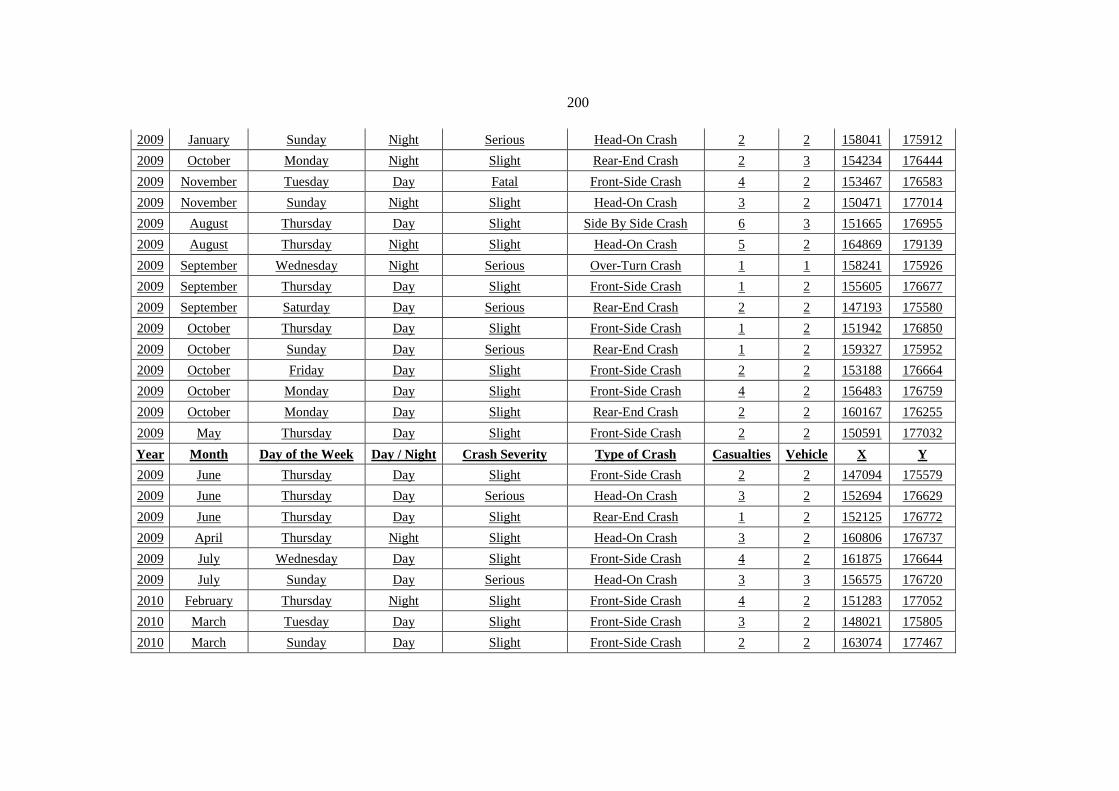
200

2009 January Sunday Night Serious Head-On Crash 2 2 158041 175912

2009 October Monday Night Slight Rear-End Crash 2 3 154234 176444

2009 November Tuesday Day Fatal Front-Side Crash 4 2 153467 176583

2009 November Sunday Night Slight Head-On Crash 3 2 150471 177014

2009 August Thursday Day Slight Side By Side Crash 6 3 151665 176955

2009 August Thursday Night Slight Head-On Crash 5 2 164869 179139

2009 September Wednesday Night Serious Over-Turn Crash 1 1 158241 175926

2009 September Thursday Day Slight Front-Side Crash 1 2 155605 176677

2009 September Saturday Day Serious Rear-End Crash 2 2 147193 175580

2009 October Thursday Day Slight Front-Side Crash 1 2 151942 176850

2009 October Sunday Day Serious Rear-End Crash 1 2 159327 175952

2009 October Friday Day Slight Front-Side Crash 2 2 153188 176664

2009 October Monday Day Slight Front-Side Crash 4 2 156483 176759

2009 October Monday Day Slight Rear-End Crash 2 2 160167 176255




2009 June Thursday Day Serious Head-On Crash 3 2 152694 176629

2009 June Thursday Day Slight Rear-End Crash 1 2 152125 176772

2009 April Thursday Night Slight Head-On Crash 3 2 160806 176737


2009 July Sunday Day Serious Head-On Crash 3 3 156575 176720

2010 February Thursday Night Slight Front-Side Crash 4 2 151283 177052



201

2010 March Sunday Night Slight Front-Side Crash 4 3 152219 176743

2010 March Wednesday Night Slight Head-On Crash 1 2 150471 177015

2010 January Sunday Night Serious Over-Turn Crash 1 1 162939 177223


2010 August Wednesday Day Slight Head-On Crash 2 2 158242 175925

2010 August Thursday Day Serious Head-On Crash 3 2 150224 176903

2010 August Wednesday Day Slight Front-Side Crash 12 2 149887 176694


2010 July Friday Night Slight Head-On Crash 2 2 152695 176627


2010 July Thursday Day Slight Front-Side Crash 2 2 150471 177015



2010 September Wednesday Night Slight Front-Side Crash 2 2 158819 175897

2010 October Sunday Day Slight Rear-End Crash 4 2 165246 179441

2010 October Friday Day Slight Side By Side Crash 1 2 166508 180407

2010 January Thursday Day Slight Front-Side Crash 1 2 151665 176956

2010 January Friday Day Slight Over-Turn Crash 1 1 155409 176646

2010 January Saturday Day Serious Front-Side Crash 2 2 153652 176514

2010 January Friday Day Slight Side By Side Crash 7 2 150691 177038

2010 February Tuesday Day Slight Head-On Crash 4 3 147392 175580

2010 March Friday Night Slight Head-On Crash 2 2 148306 175949

2010 April Wednesday Day Slight Front-Side Crash 2 2 160427 176631



202

2010 May Friday Night Slight Front-Side Crash 2 2 158820 175898

2010 December Monday Day Serious Front-Side Crash 2 3 148567 176027

2010 December Thursday Night Slight Rear-End Crash 1 2 148306 175949



2010 October Tuesday Day Slight Front-Side Crash 2 2 149803 176643

2010 October Wednesday Night Serious Side By Side Crash 1 2 149032 176198

2010 November Sunday Day Slight Front-Side Crash 1 2 157541 175910


2010 November Thursday Day Slight Head-On Crash 6 2 150471 177015

2010 November Wednesday Day Serious Over-Turn Crash 2 1 164662 178779

2010 December Wednesday Day Slight Front-Side Crash 2 2 150987 177065

2010 August Friday Day Slight Rear-End Crash 1 3 152602 176664

2010 August Sunday Night Slight Head-On Crash 2 2 164476 178731

2010 August Sunday Night Fatal Side By Side Crash 6 3 164182 178473

2010 May Thursday Day Slight Head-On Crash 5 2 150471 177015

2010 May Thursday Night Slight Side By Side Crash 1 2 153082 176662

2010 May Monday Night Slight Front-Side Crash 3 2 149380 176385

2010 June Saturday Night Slight Skidding Crash 1 1 154528 176495


2011 February Saturday Day Slight Front-Side Crash 1 2 148306 175952.5

2011 February Wednesday Day Slight Head-On Crash 5 2 157541 175909


2011 February Thursday Day Slight Front-Side Crash 3 2 166750 180305.5

2011 March Wednesday Night Slight Side By Side Crash 3 3 158141 175919.7

203

2011 March Thursday Night Slight Over-Turn Crash 5 1 151183 177064



2011 June Monday Day Slight Front-Side Crash 2 2 152127 176773

2011 July Friday Day Slight Front-Side Crash 4 2 152602 176664



2011 August Monday Day Slight Rear-End Crash 6 2 147095 175579


2011 October Tuesday Day Fatal Head-On Crash 2 2 160805 176736

2011 October Monday Night Slight Head-On Crash 3 2 150223 176904

2011 August Thursday Night Slight Front-Side Crash 1 2 155017 176578

2011 September Monday Night Slight Rear-End Crash 2 3 151665 176957



2011 September Saturday Day Slight Head-On Crash 6 2 150691 177037



2011 October Friday Night Serious Head-On Crash 5 2 156659 176668


2011 November Sunday Night Slight Side By Side Crash 2 2 162596 176796



2011 December Saturday Day Serious Head-On Crash 5 2 153188 176664

2011 December Sunday Night Slight Rear-End Crash 1 2 147093 175578

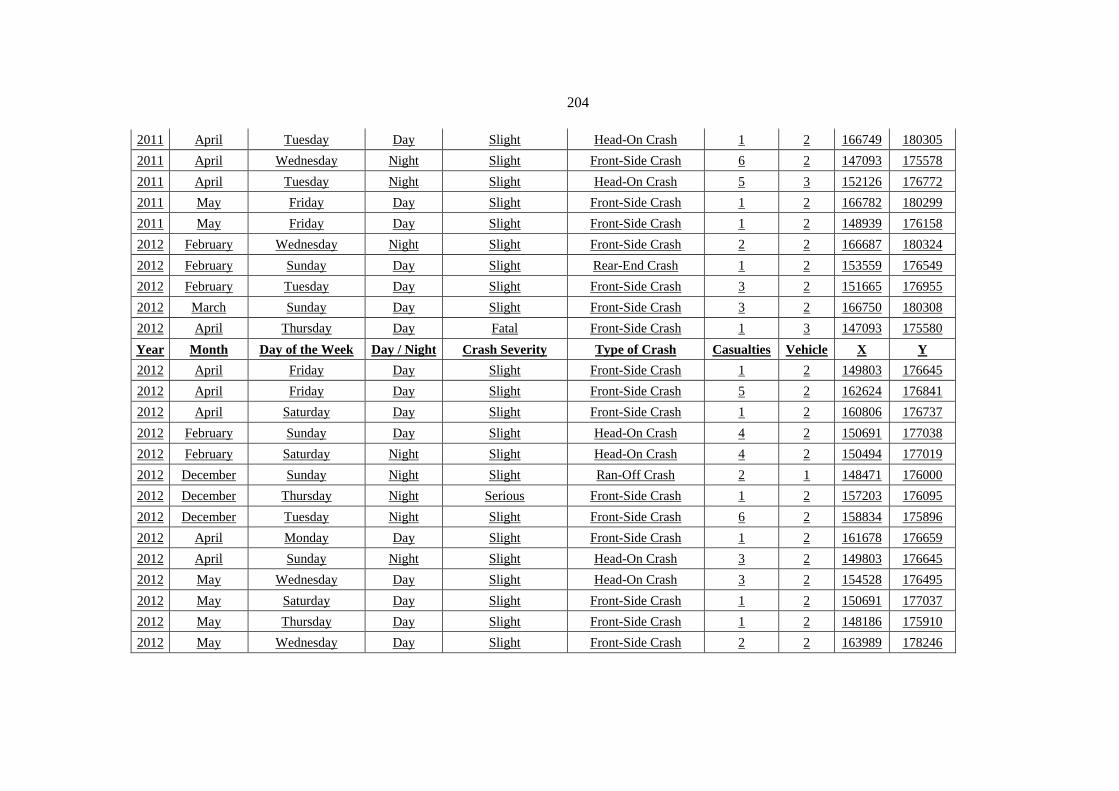
204

2011 April Tuesday Day Slight Head-On Crash 1 2 166749 180305

2011 April Wednesday Night Slight Front-Side Crash 6 2 147093 175578

2011 April Tuesday Night Slight Head-On Crash 5 3 152126 176772

2011 May Friday Day Slight Front-Side Crash 1 2 166782 180299



2012 February Sunday Day Slight Rear-End Crash 1 2 153559 176549

2012 February Tuesday Day Slight Front-Side Crash 3 2 151665 176955


2012 April Thursday Day Fatal Front-Side Crash 1 3 147093 175580


2012 April Friday Day Slight Front-Side Crash 1 2 149803 176645

2012 April Friday Day Slight Front-Side Crash 5 2 162624 176841

2012 April Saturday Day Slight Front-Side Crash 1 2 160806 176737

2012 February Sunday Day Slight Head-On Crash 4 2 150691 177038

2012 February Saturday Night Slight Head-On Crash 4 2 150494 177019

2012 December Sunday Night Slight Ran-Off Crash 2 1 148471 176000

2012 December Thursday Night Serious Front-Side Crash 1 2 157203 176095

2012 December Tuesday Night Slight Front-Side Crash 6 2 158834 175896


2012 April Sunday Night Slight Head-On Crash 3 2 149803 176645

2012 May Wednesday Day Slight Head-On Crash 3 2 154528 176495

2012 May Saturday Day Slight Front-Side Crash 1 2 150691 177037


2012 May Wednesday Day Slight Front-Side Crash 2 2 163989 178246

205

2012 May Sunday Day Slight Front-Side Crash 5 2 163074 177466





2012 June Wednesday Day Serious Head-On Crash 6 2 165246 179439

2012 July Thursday Day Serious Front-Side Crash 1 3 148938 176159



2012 September Thursday Day Slight Rear-End Crash 1 3 157204 176093

2012 September Monday Day Slight Head-On Crash 3 2 150222 176902

2012 October Tuesday Day Slight Over-Turn Crash 1 1 157203 176094

2012 October Thursday Night Slight Front-Side Crash 1 2 151667 176955


2012 August Sunday Day Slight Front-Side Crash 1 2 159608 176048


2012 August Monday Night Slight Side By Side Crash 1 2 154528 176496


2012 November Thursday Day Slight Ran-Off Crash 1 1 152601 176665

2012 November Sunday Day Slight Side By Side Crash 2 2 149803 176645


206

Table B.2: Crash Data for Highway 60 ( Nablus to Hebron Road)




2003 December Friday Day Slight Side By Side Crash 3 2 174445 170704

2003 April Saturday Night Fatal Over-Turn Crash 2 1 174516 172317


2003 January Tuesday Day Slight Front-Side Crash 5 2 167911 185636


2003 January Wednesday Night Slight Front-Side Crash 5 3 173924 156082

2003 November Friday Day Slight Ran-Off Crash 2 1 174454 169531

2004 August Wednesday Day Slight Over-Turn Crash 7 1 174315 152459

2004 August Thursday Day Slight Head-On Crash 4 2 173398 167390

2004 August Thursday Day Slight Front-Side Crash 6 2 174694 165207




2004 May Friday Night Slight Over-Turn Crash 3 1 174897 174449




2004 July Friday Night Fatal Front-Side Crash 4 2 174700 173810

2004 July Tuesday Day Slight Side By Side Crash 1 2 174522 171394

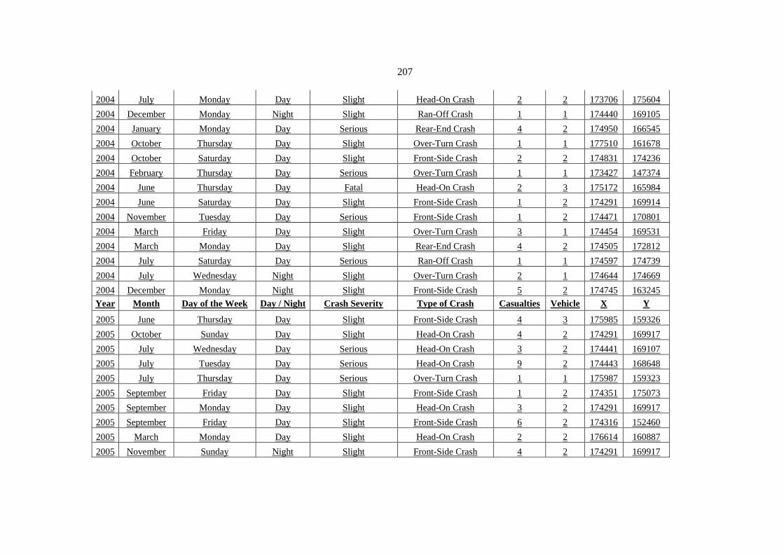
207

2004 July Monday Day Slight Head-On Crash 2 2 173706 175604

2004 December Monday Night Slight Ran-Off Crash 1 1 174440 169105

2004 January Monday Day Serious Rear-End Crash 4 2 174950 166545

2004 October Thursday Day Slight Over-Turn Crash 1 1 177510 161678

2004 October Saturday Day Slight Front-Side Crash 2 2 174831 174236

2004 February Thursday Day Serious Over-Turn Crash 1 1 173427 147374

2004 June Thursday Day Fatal Head-On Crash 2 3 175172 165984

2004 June Saturday Day Slight Front-Side Crash 1 2 174291 169914

2004 November Tuesday Day Serious Front-Side Crash 1 2 174471 170801

2004 March Friday Day Slight Over-Turn Crash 3 1 174454 169531

2004 March Monday Day Slight Rear-End Crash 4 2 174505 172812

2004 July Saturday Day Serious Ran-Off Crash 1 1 174597 174739

2004 July Wednesday Night Slight Over-Turn Crash 2 1 174644 174669

2004 December Monday Night Slight Front-Side Crash 5 2 174745 163245



2005 October Sunday Day Slight Head-On Crash 4 2 174291 169917

2005 July Wednesday Day Serious Head-On Crash 3 2 174441 169107

2005 July Tuesday Day Serious Head-On Crash 9 2 174443 168648

2005 July Thursday Day Serious Over-Turn Crash 1 1 175987 159323




2005 March Monday Day Slight Head-On Crash 2 2 176614 160887


208

2005 February Thursday Night Slight Front-Side Crash 1 2 174023 175332


2005 December Friday Day Fatal Front-Side Crash 3 2 174270 163243

2005 December Thursday Night Slight Side By Side Crash 2 4 173718 164571

2005 March Thursday Night Slight Rear-End Crash 3 2 174831 174239


2005 August Saturday Day Slight Front-Side Crash 4 2 173399 167390

2005 August Friday Day Slight Rear-End Crash 10 2 174515 171523


2005 January Thursday Night Fatal Head-On Crash 4 4 173964 153416

2005 June Sunday Day Slight Over-Turn Crash 1 1 174291 169916



2006 January Tuesday Day Slight Ran-Off Crash 3 1 166748 180307




2006 January Monday Night Serious Front-Side Crash 6 2 174450 150743

2006 July Tuesday Day Slight Over-Turn Crash 1 1 173493 167006

2006 April Monday Day Fatal Head-On Crash 8 2 175985 159327

2006 April Friday Day Slight Head-On Crash 4 2 175985 159327

2006 September Tuesday Day Slight Head-On Crash 4 2 173923 156083




209

2006 August Friday Day Slight Head-On Crash 1 3 174498 171097

2006 August Friday Day Slight Over-Turn Crash 1 1 174351 175075




2006 October Wednesday Day Serious Side By Side Crash 8 2 166748 180307

2006 January Sunday Night Slight Over-Turn Crash 1 1 174511 172848

2006 May Wednesday Night Fatal Head-On Crash 11 2 174000 164712

2006 May Tuesday Day Slight Front-Side Crash 3 2 174510 172424

2006 March Monday Day Slight Over-Turn Crash 5 1 174510 167007

2006 September Saturday Night Slight Over-Turn Crash 4 1 173872 167891

2006 July Tuesday Day Fatal Over-Turn Crash 2 2 166748 180307

2006 July Tuesday Day Slight Rear-End Crash 1 2 174510 171786

2006 July Friday Day Slight Side By Side Crash 6 2 174639 173484


2007 March Tuesday Day Serious Rear-End Crash 2 2 173629 148280

2007 March Sunday Night Slight Rear-End Crash 1 2 174619 173375

2007 March Saturday Night Slight Head-On Crash 3 2 174291 169917

2007 April Monday Day Slight Rear-End Crash 1 2 175378 158541

2007 September Monday Day Slight Front-Side Crash 2 2 174440 169179

2007 January Monday Day Serious Rear-End Crash 2 3 174521 171395


2007 June Tuesday Day Slight Rear-End Crash 3 2 173427 147374

2007 October Tuesday Day Slight Head-On Crash 6 2 174296 166786

2007 October Saturday Night Slight Front-Side Crash 6 2 173489 163560

210

2007 July Sunday Day Slight Head-On Crash 2 2 173716 155213

2007 December Thursday Day Slight Rear-End Crash 2 2 173398 167390

2007 November Thursday Day Slight Rear-End Crash 9 2 173398 167390

2007 November Friday Day Slight Over-Turn Crash 2 1 174896 174451

2007 March Tuesday Day Slight Head-On Crash 3 2 174432 169710



2007 August Thursday Day Slight Rear-End Crash 4 2 174512 171908

2007 August Saturday Day Slight Rear-End Crash 4 2 174523 171292

2007 July Friday Day Slight Head-On Crash 1 2 175022 157604


2007 January Sunday Day Slight Head-On Crash 3 2 174897 174449


2007 May Thursday Day Serious Front-Side Crash 4 2 175985 159326

2007 May Monday Day Slight Head-On Crash 2 2 173398 167390



2007 October Friday Day Slight Head-On Crash 2 2 174502 174875

2008 August Friday Night Slight Over-Turn Crash 3 1 145704 84135






2008 August Wednesday Day Slight Rear-End Crash 1 3 167911 185634

211

2008 August Wednesday Day Fatal Head-On Crash 2 2 165177 123649


2008 August Thursday Day Serious Head-On Crash 2 2 174502 174875



2008 January Wednesday Night Serious Front-Side Crash 3 2 163743 117898

2008 January Monday Night Slight Rear-End Crash 1 2 169597 126527

2008 July Monday Day Slight Rear-End Crash 2 2 174000 164708



2008 July Wednesday Day Serious Front-Side Crash 2 2 174645 174666



2008 November Saturday Night Fatal Head-On Crash 9 2 162535 116518

2008 November Sunday Night Serious Skidding Crash 1 1 160567 111432

2008 December Wednesday Day Slight Head-On Crash 2 2 161410 108363

2008 December Wednesday Day Slight Head-On Crash 1 4 160443 111499

2008 December Sunday Day Slight Over-Turn Crash 1 1 160814 113167


2008 March Monday Day Slight Front-Side Crash 1 2 163548 117698

2008 March Thursday Day Slight Over-Turn Crash 6 1 153386 92482

2008 March Thursday Day Serious Front-Side Crash 3 2 177512 161679

2008 March Tuesday Night Serious Head-On Crash 3 2 177512 161679

2008 March Sunday Night Slight Rear-End Crash 1 4 174510 172426

2008 August Tuesday Night Slight Over-Turn Crash 2 1 166750 180306

212

2008 August Thursday Night Slight Rear-End Crash 2 2 162677 117203

2008 September Friday Day Serious Front-Side Crash 2 2 166477 124496



2008 September Friday Day Serious Front-Side Crash 8 2 163621 119516

2008 September Monday Day Slight Over-Turn Crash 3 1 174398 170314

2008 February Monday Day Slight Rear-End Crash 2 2 165153 121146

2008 February Monday Day Slight Head-On Crash 2 2 174761 174550

2008 February Monday Day Slight Over-Turn Crash 1 1 166750 180307

2008 June Sunday Day Slight Head-On Crash 3 2 173399 167390

2008 June Wednesday Day Fatal Front-Side Crash 3 2 161186 110468


2008 November Wednesday Day Serious Front-Side Crash 2 2 160567 111432

2008 November Wednesday Day Slight Side By Side Crash 1 2 174761 174550

2008 November Tuesday Day Slight Ran-Off Crash 3 1 153397 91546

2008 November Thursday Day Slight Front-Side Crash 6 3 165005 123466

2008 November Thursday Night Slight Side By Side Crash 1 2 163549 117698


2008 November Tuesday Night Slight Front-Side Crash 5 2 152020 94884

2008 November Thursday Night Slight Front-Side Crash 2 2 165004 123464




2008 September Friday Day Slight Head-On Crash 4 2 162350 114671

2008 September Wednesday Day Slight Head-On Crash 1 2 160745 112687

213



2008 September Wednesday Day Serious Head-On Crash 4 2 176336 163276



2008 April Wednesday Night Serious Front-Side Crash 3 2 174515 166773


2008 September Friday Night Slight Front-Side Crash 6 2 165176 121508

2008 September Saturday Night Slight Rear-End Crash 6 2 174511 171803

2008 September Tuesday Night Serious Over-Turn Crash 2 1 173717 155215

2008 October Wednesday Night Serious Front-Side Crash 3 2 165175 121511


2008 October Thursday Day Slight Head-On Crash 8 3 174432 169705

2008 April Sunday Night Slight Head-On Crash 6 2 174952 140199




2008 July Sunday Night Slight Front-Side Crash 1 2 163549 117698

2008 July Thursday Night Slight Front-Side Crash 4 2 162585 117094


2008 December Wednesday Night Slight Head-On Crash 3 2 160567 111432

2008 January Thursday Day Slight Rear-End Crash 1 2 165267 122284

2008 January Tuesday Day Serious Rear-End Crash 5 2 173492 167009

2008 January Tuesday Day Slight Side By Side Crash 1 2 162711 102367

2008 January Tuesday Day Slight Over-Turn Crash 3 1 173579 164297

214



2008 October Thursday Night Serious Rear-End Crash 4 3 174897 174515

2008 October Sunday Night Slight Rear-End Crash 2 2 163549 117698


2008 November Friday Day Slight Side By Side Crash 1 2 174387 169781

2008 November Thursday Day Slight Head-On Crash 2 2 164552 120916



2009 February Saturday Night Fatal Front-Side Crash 4 3 175985 159328


2009 February Monday Night Slight Front-Side Crash 2 2 176276 143826

2009 February Wednesday Day Slight Over-Turn Crash 1 1 175125 142385

2009 February Sunday Day Serious Front-Side Crash 1 2 163549 117699

2009 January Sunday Day Slight Side By Side Crash 3 2 174744 163244

2009 January Thursday Day Slight Head-On Crash 2 2 163860 118787

2009 January Saturday Night Slight Front-Side Crash 5 2 161377 108068

2009 March Saturday Day Slight Front-Side Crash 1 2 163548 117700


2009 March Sunday Day Fatal Head-On Crash 9 2 163563 119590

2009 March Friday Day Slight Front-Side Crash 6 2 165007 123467

2009 March Sunday Day Slight Head-On Crash 2 2 145703 84134

2009 March Wednesday Day Slight Rear-End Crash 1 2 166002 184838


2009 June Wednesday Day Slight Head-On Crash 5 3 164917 122403

215

2009 June Thursday Day Slight Head-On Crash 3 2 174744 163245

2009 July Wednesday Day Slight Rear-End Crash 2 2 173716 155215




2009 June Friday Day Fatal Front-Side Crash 9 2 164488 120848

2009 June Friday Day Slight Front-Side Crash 1 2 166311 182488

2009 June Saturday Day Slight Ran-Off Crash 1 1 160773 112779



2009 March Wednesday Night Slight Front-Side Crash 2 2 165267 122284

2009 April Friday Day Slight Over-Turn Crash 5 2 171610 139602

2009 April Sunday Day Slight Skidding Crash 6 1 149842 86975

2009 February Wednesday Day Serious Head-On Crash 5 2 174962 157522

2009 February Sunday Day Slight Front-Side Crash 3 2 174619 173375

2009 February Wednesday Day Slight Head-On Crash 1 2 161664 107799


2009 February Tuesday Day Slight Side By Side Crash 4 2 165177 123615

2009 July Friday Day Serious Side By Side Crash 9 2 161097 114064

2009 July Sunday Day Serious Front-Side Crash 5 2 152062 94963


2009 July Thursday Day Serious Head-On Crash 2 2 161493 114334

2009 July Wednesday Day Slight Side By Side Crash 4 2 174450 150743


2009 December Tuesday Day Slight Rear-End Crash 2 3 165916 184604

216

2009 December Sunday Night Slight Front-Side Crash 4 2 167910 185636

2009 December Friday Night Slight Front-Side Crash 5 2 165177 121509



2009 April Saturday Night Slight Front-Side Crash 3 2 170771 128447

2009 April Saturday Night Fatal Front-Side Crash 3 3 167911 185638

2009 April Sunday Night Slight Front-Side Crash 3 2 174744 163246

2009 April Thursday Night Slight Head-On Crash 5 3 176276 143828

2009 September Monday Night Slight Front-Side Crash 4 2 175990 159225

2009 October Wednesday Day Slight Front-Side Crash 2 2 174451 150742


2009 October Tuesday Day Slight Head-On Crash 6 2 162181 109406




2009 May Monday Day Serious Head-On Crash 1 2 165005 123457





2009 October Sunday Night Slight Front-Side Crash 1 2 147995 86121


2009 October Wednesday Night Slight Front-Side Crash 1 2 175530 142965

2009 October Tuesday Night Slight Front-Side Crash 2 2 166161 123736

2009 October Saturday Night Slight Over-Turn Crash 1 1 174464 169444

217

2009 November Sunday Night Slight Over-Turn Crash 3 1 173768 175548

2009 November Tuesday Day Serious Head-On Crash 1 2 162120 109536

2009 May Thursday Night Slight Front-Side Crash 5 2 173397 167391

2009 June Monday Night Slight Front-Side Crash 4 2 161081 100940




2009 September Monday Day Serious Head-On Crash 5 2 174199 156906


2009 September Tuesday Day Slight Side By Side Crash 1 2 165343 122231




2009 September Thursday Night Slight Head-On Crash 3 2 175087 165617

2009 September Tuesday Night Slight Front-Side Crash 1 2 161502 108468


2009 August Saturday Day Slight Side By Side Crash 1 2 163691 117817



2009 December Monday Night Slight Head-On Crash 5 2 152020 94884






218


2009 November Thursday Day Slight Front-Side Crash 3 2 176276 143826

2009 November Thursday Day Serious Side By Side Crash 2 2 163621 119518

2009 November Thursday Day Fatal Head-On Crash 13 3 163621 119518

2009 November Thursday Night Slight Front-Side Crash 4 2 160774 112777




2009 November Tuesday Night Slight Head-On Crash 4 2 174270 163243

2009 December Thursday Night Slight Head-On Crash 3 3 175713 158804


2010 February Saturday Day Slight Front-Side Crash 4 2 160927 113633


2010 March Monday Night Slight Over-Turn Crash 2 3 170053 177338

2010 March Tuesday Night Slight Front-Side Crash 1 2 174951 140200

2010 April Tuesday Night Serious Over-Turn Crash 1 1 145704 84134

2010 May Sunday Day Slight Rear-End Crash 4 3 153238 90478


2010 May Monday Day Slight Front-Side Crash 1 2 174951 140197



2010 May Sunday Day Serious Head-On Crash 2 3 160374 111622

2010 May Wednesday Day Slight Over-Turn Crash 1 1 175713 158803

2010 January Monday Day Slight Over-Turn Crash 4 1 174640 173482


219

2010 January Monday Day Serious Head-On Crash 3 2 166404 124329

2010 January Saturday Day Serious Over-Turn Crash 5 1 152249 93856

2010 January Monday Day Serious Front-Side Crash 7 2 175097 157999

2010 January Saturday Day Slight Front-Side Crash 2 2 165196 121540



2010 June Wednesday Day Slight Head-On Crash 1 2 174510 172426


2010 July Tuesday Night Slight Head-On Crash 1 2 174954 140197

2010 July Monday Day Slight Head-On Crash 2 2 162459 103661

2010 July Tuesday Day Slight Rear-End Crash 4 3 174764 165271

2010 April Thursday Day Slight Front-Side Crash 3 2 174954 140197

2010 April Wednesday Night Slight Ran-Off Crash 1 1 174453 169532

2010 April Saturday Night Slight Head-On Crash 2 2 154604 98843

2010 April Monday Night Slight Rear-End Crash 6 2 162534 116518


2010 September Saturday Day Slight Front-Side Crash 2 2 166086 123682

2010 September Saturday Night Slight Rear-End Crash 3 2 164490 120848


2010 April Thursday Night Serious Head-On Crash 6 2 175738 143193

2010 April Sunday Day Slight Head-On Crash 2 2 153397 91544


2010 April Friday Day Serious Front-Side Crash 4 2 176627 143828



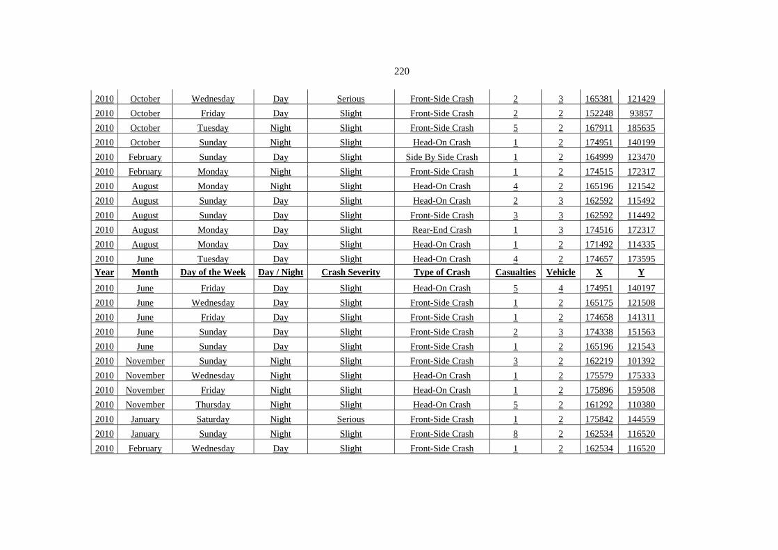
220

2010 October Wednesday Day Serious Front-Side Crash 2 3 165381 121429


2010 October Tuesday Night Slight Front-Side Crash 5 2 167911 185635

2010 October Sunday Night Slight Head-On Crash 1 2 174951 140199

2010 February Sunday Day Slight Side By Side Crash 1 2 164999 123470


2010 August Monday Night Slight Head-On Crash 4 2 165196 121542

2010 August Sunday Day Slight Head-On Crash 2 3 162592 115492




2010 June Tuesday Day Slight Head-On Crash 4 2 174657 173595


2010 June Friday Day Slight Head-On Crash 5 4 174951 140197



2010 June Sunday Day Slight Front-Side Crash 2 3 174338 151563



2010 November Wednesday Night Slight Head-On Crash 1 2 175579 175333

2010 November Friday Night Slight Head-On Crash 1 2 175896 159508

2010 November Thursday Night Slight Head-On Crash 5 2 161292 110380

2010 January Saturday Night Serious Front-Side Crash 1 2 175842 144559



221








2010 July Tuesday Night Serious Front-Side Crash 5 2 173840 140177

2010 March Thursday Day Slight Front-Side Crash 3 2 173398 167391



2010 August Wednesday Night Slight Side By Side Crash 4 2 173997 153331

2010 September Thursday Night Slight Front-Side Crash 7 2 175187 140293

2010 September Friday Night Slight Front-Side Crash 1 2 162350 114668

2010 September Saturday Night Slight Front-Side Crash 1 2 164621 120980


2010 September Sunday Day Slight Head-On Crash 6 2 174952 140199

2010 October Friday Night Slight Head-On Crash 5 2 172330 140625

2010 October Sunday Day Slight Head-On Crash 1 2 174952 140199

2010 December Sunday Day Slight Head-On Crash 2 2 174952 140199


2010 December Monday Day Slight Rear-End Crash 5 2 161054 111027



2010 December Friday Day Slight Rear-End Crash 1 2 162534 116517

222


2010 December Tuesday Night Slight Head-On Crash 8 2 174439 169001


2010 December Saturday Night Slight Front-Side Crash 8 2 175674 143125

2010 December Saturday Night Slight Rear-End Crash 13 4 164488 120851


2010 May Tuesday Day Slight Over-Turn Crash 2 1 174267 150232

2010 May Monday Night Slight Side By Side Crash 6 2 152248 93858

2011 January Thursday Day Slight Rear-End Crash 2 2 174498 171097


2011 January Thursday Day Slight Skidding Crash 1 1 174548 141764


2011 January Thursday Night Fatal Front-Side Crash 6 2 174222 145945

2011 February Tuesday Night Slight Head-On Crash 2 2 174954 140197

2011 March Tuesday Day Slight Skidding Crash 3 1 166477 124498

2011 March Tuesday Day Slight Skidding Crash 3 1 166477 124498

2011 March Thursday Day Slight Rear-End Crash 1 2 164488 120851

2011 February Friday Day Slight Head-On Crash 4 2 174338 151563

2011 February Thursday Day Slight Front-Side Crash 2 2 165196 121542


2011 February Wednesday Day Slight Side By Side Crash 3 2 175990 159226

2011 February Saturday Day Slight Front-Side Crash 2 2 166266 123887

2011 February Friday Day Serious Front-Side Crash 1 2 163861 118787

2011 February Thursday Day Slight Front-Side Crash 3 2 166748 180306


223

2011 February Saturday Night Fatal Head-On Crash 7 4 174047 163261

2011 June Sunday Day Serious Over-Turn Crash 1 2 163907 120166


2011 June Saturday Day Fatal Head-On Crash 4 2 177170 162587





2011 April Saturday Night Slight Head-On Crash 2 4 160926 113634

2011 April Sunday Day Slight Over-Turn Crash 2 1 152019 94886

2011 April Sunday Day Slight Front-Side Crash 2 2 161875 110052


2011 April Wednesday Day Serious Head-On Crash 5 7 175096 158002




2011 July Saturday Day Slight Skidding Crash 3 2 149842 86975


2011 July Monday Day Slight Side By Side Crash 3 2 174659 141313

2011 July Sunday Day Slight Head-On Crash 1 2 162534 116520

2011 July Saturday Day Slight Front-Side Crash 5 3 161377 108068

2011 April Wednesday Day Slight Head-On Crash 8 2 177486 161542

2011 April Tuesday Day Slight Head-On Crash 1 2 166748 180306


2011 April Tuesday Night Slight Front-Side Crash 4 2 174954 140197

224


2011 July Sunday Night Slight Head-On Crash 2 2 174451 150653

2011 July Thursday Night Fatal Head-On Crash 8 2 173717 155121


2011 August Tuesday Day Slight Head-On Crash 1 2 160567 111434


2011 May Sunday Day Slight Side By Side Crash 6 2 168663 177521



2011 May Tuesday Day Slight Head-On Crash 2 2 163861 118788

2011 May Monday Day Serious Front-Side Crash 2 2 161142 110604



2011 May Tuesday Day Fatal Head-On Crash 5 2 163621 119518

2011 May Sunday Day Slight Over-Turn Crash 1 1 159781 100651



2011 September Thursday Day Slight Head-On Crash 2 2 174954 140197

2011 September Thursday Night Slight Front-Side Crash 1 2 174954 140197



2011 August Monday Night Slight Front-Side Crash 1 2 172461 137158

2011 September Monday Night Slight Over-Turn Crash 3 1 153237 90477



225



2011 September Friday Day Fatal Head-On Crash 4 2 162350 114670

2011 September Wednesday Day Slight Head-On Crash 2 2 174954 140197

2011 January Friday Night Serious Head-On Crash 7 2 165196 121544

2011 January Sunday Night Slight Skidding Crash 2 1 175675 143126

2011 February Friday Night Slight Head-On Crash 1 2 173790 149548

2011 February Friday Day Slight Head-On Crash 2 2 173996 153332

2011 May Tuesday Day Slight Over-Turn Crash 2 1 173715 155400

2011 June Thursday Night Slight Head-On Crash 3 2 174954 140197

2011 June Sunday Day Slight Head-On Crash 6 2 173715 143058

2011 June Friday Day Slight Side By Side Crash 4 3 172700 135545

2011 June Friday Day Serious Head-On Crash 6 3 174761 174552

2011 June Monday Day Slight Head-On Crash 1 2 174002 149853

2011 November Friday Night Slight Head-On Crash 4 2 171438 140660

2011 November Wednesday Night Slight Rear-End Crash 2 2 163908 118698

2011 December Sunday Night Slight Head-On Crash 3 3 166477 124498



2011 January Friday Day Slight Over-Turn Crash 5 1 176614 160887


2011 October Tuesday Night Slight Side By Side Crash 2 2 161292 110380

2011 November Friday Night Slight Side By Side Crash 1 2 174150 156808

2011 November Monday Day Slight Front-Side Crash 2 2 172461 137158

2011 November Sunday Day Fatal Head-On Crash 2 2 165343 122231

226


2011 November Tuesday Night Slight Head-On Crash 3 2 174954 140197

2011 July Friday Day Slight Head-On Crash 5 3 174199 166795


2011 July Monday Day Serious Head-On Crash 6 2 162623 105002


2011 December Friday Day Slight Head-On Crash 1 2 174954 140197


2011 December Friday Day Serious Front-Side Crash 1 2 164488 120852

2011 December Thursday Night Slight Head-On Crash 2 2 171439 140660



2011 March Monday Day Slight Head-On Crash 1 2 152310 95721




2011 October Wednesday Day Slight Head-On Crash 2 2 175676 143125

2011 October Wednesday Day Slight Head-On Crash 8 3 162622 105003

2011 October Thursday Night Serious Over-Turn Crash 2 1 174694 165210

2011 October Saturday Night Serious Head-On Crash 5 2 175990 159228


2011 August Saturday Day Slight Rear-End Crash 2 3 174511 171805

2011 June Sunday Day Serious Over-Turn Crash 1 1 145704 84136

2011 June Thursday Day Slight Head-On Crash 2 4 149842 86975

2011 June Wednesday Night Slight Front-Side Crash 4 2 174516 172318

227


2012 February Saturday Night Slight Head-On Crash 2 2 165153 121458

2012 February Sunday Night Slight Head-On Crash 1 2 174954 140197

2012 February Wednesday Day Slight Side By Side Crash 1 2 175114 145132


2012 January Friday Day Slight Front-Side Crash 1 2 165153 121461


2012 January Tuesday Day Slight Front-Side Crash 3 4 174350 175073


2012 April Friday Night Slight Front-Side Crash 3 2 172461 137158


2012 April Wednesday Day Slight Head-On Crash 3 2 173872 167891






2012 May Sunday Day Slight Side By Side Crash 4 2 161292 110382






2012 March Friday Day Slight Front-Side Crash 3 2 163549 117698


228




2012 March Wednesday Day Slight Over-Turn Crash 5 1 165343 122234

2012 March Friday Day Serious Front-Side Crash 3 2 172461 137158


2012 January Saturday Day Slight Head-On Crash 1 3 164999 123470

2012 January Friday Day Slight Head-On Crash 6 2 174394 151740


2012 January Tuesday Night Slight Front-Side Crash 2 2 174954 140197

2012 January Saturday Night Slight Front-Side Crash 2 2 160926 113633

2012 January Thursday Night Serious Front-Side Crash 2 2 174577 173162

2012 January Saturday Night Slight Head-On Crash 4 2 174750 140139



2012 June Wednesday Day Serious Head-On Crash 2 3 154603 98846

2012 June Saturday Day Slight Over-Turn Crash 16 1 171206 129497



2012 June Monday Day Serious Head-On Crash 2 3 163909 118700





2012 August Friday Day Fatal Head-On Crash 6 4 171573 131590

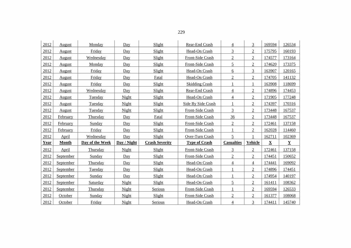
229






2012 August Friday Day Fatal Head-On Crash 2 2 174705 141132

2012 August Friday Day Slight Skidding Crash 1 1 163908 118699


2012 August Tuesday Night Slight Head-On Crash 4 2 171905 177248

2012 August Tuesday Night Slight Side By Side Crash 1 2 174397 170316


2012 February Thursday Day Fatal Front-Side Crash 36 2 173448 167537


2012 February Friday Day Slight Front-Side Crash 1 2 162028 114460

2012 April Wednesday Day Slight Over-Turn Crash 5 1 162711 102369


2012 April Thursday Night Slight Front-Side Crash 3 2 172461 137158

2012 September Sunday Day Slight Front-Side Crash 2 2 174451 150652



2012 September Sunday Day Slight Head-On Crash 1 2 174954 140197

2012 September Saturday Night Slight Head-On Crash 5 2 161411 108362

2012 September Thursday Night Serious Front-Side Crash 1 2 169594 126533


2012 October Friday Night Serious Head-On Crash 4 3 174411 145740

230

2012 October Friday Day Serious Head-On Crash 3 2 174316 157098

2012 October Monday Day Slight Head-On Crash 3 2 168744 126042

2012 October Saturday Day Serious Head-On Crash 8 3 165013 121223

2012 October Sunday Day Slight Front-Side Crash 1 2 174578 173165

2012 October Friday Day Slight Rear-End Crash 4 2 175172 165986

2012 October Saturday Day Serious Front-Side Crash 6 2 174577 173165

2012 October Tuesday Day Slight Front-Side Crash 1 2 164488 120850


2012 October Tuesday Day Serious Front-Side Crash 4 2 168745 126040


2012 October Friday Night Slight Over-Turn Crash 2 1 169594 126535



2012 May Saturday Night Slight Head-On Crash 5 2 174954 140197


2012 June Sunday Night Slight Over-Turn Crash 1 1 152027 94380

2012 December Thursday Day Slight Front-Side Crash 5 3 174954 140197




2012 December Saturday Night Slight Rear-End Crash 6 4 174443 168648





231

2012 December Monday Night Fatal Head-On Crash 3 2 162459 103665






2012 June Monday Night Slight Head-On Crash 5 3 173687 154208

2012 October Thursday Night Slight Head-On Crash 5 2 172461 137158


2012 October Tuesday Night Serious Head-On Crash 1 2 162592 115492

2012 November Sunday Night Slight Over-Turn Crash 2 1 152751 93012


2012 November Monday Day Fatal Skidding Crash 1 2 166825 124810

2012 November Thursday Day Serious Front-Side Crash 6 2 174451 150652

2012 November Saturday Night Slight Front-Side Crash 1 2 166086 123682

2012 November Wednesday Day Slight Rear-End Crash 3 2 165177 123652

2012 July Tuesday Night Serious Front-Side Crash 5 2 176299 143918

2012 July Wednesday Night Slight Over-Turn Crash 4 1 174411 145738




2012 July Tuesday Day Slight Head-On Crash 1 3 174620 173374



2012 July Friday Day Serious Skidding Crash 1 1 174824 142185

232


2012 December Sunday Day Slight Rear-End Crash 2 2 163549 117698

2012 August Tuesday Night Serious Head-On Crash 2 2 174002 149852

2012 September Wednesday Night Slight Ran-Off Crash 1 1 169594 126530


2012 July Wednesday Night Slight Front-Side Crash 4 2 172461 137158

2012 July Sunday Night Slight Front-Side Crash 5 2 172461 137158

2012 July Saturday Night Slight Rear-End Crash 5 2 162459 103663

2012 July Saturday Night Serious Head-On Crash 3 3 162819 106418

2012 August Wednesday Night Slight Head-On Crash 1 3 161572 110317

2012 August Sunday Night Slight Front-Side Crash 9 2 172461 137158


2012 August Wednesday Night Slight Front-Side Crash 1 2 172461 137158

2012 August Friday Day Slight Front-Side Crash 3 2 165196 121543

233

Table B.3: Crash Data for Highway 505 ( Salfit to Za'tara Road)


2008 September Saturday Day Slight Over-Turn Crash 1 1 168362 169442

2008 September Tuesday Day Slight Rear-End Crash 2 2 181104 169649

2008 September Thursday Day Slight Rear-End Crash 1 2 166855 168667

2008 July Friday Day Slight Rear-End Crash 1 2 165805 168393


2008 July Monday Day Slight Ran-Off Crash 4 1 167779 169039

2008 August Tuesday Day Slight Over-Turn Crash 2 1 182409 168167




2008 June Wednesday Night Slight Front-Side Crash 4 2 167528 168864

2008 May Wednesday Night Slight Over-Turn Crash 1 1 181105 169651

2008 May Thursday Day Slight Side By Side Crash 3 2 170091 169938

2008 January Wednesday Day Serious Rear-End Crash 2 2 168361 169445

2008 September Monday Night Slight Front-Side Crash 1 2 182772 167218




2009 April Friday Day Slight Rear-End Crash 1 2 169889 169931

2009 February Tuesday Day Serious Over-Turn Crash 1 2 165805 168393

2009 December Sunday Day Fatal Over-Turn Crash 1 1 176143 169351

2009 November Sunday Night Slight Skidding Crash 1 1 176143 169350

234



2010 March Friday Night Slight Rear-End Crash 4 3 183549 164435

2010 February Tuesday Night Slight Front-Side Crash 2 2 183549 164435

2010 June Thursday Day Serious Front-Side Crash 3 2 170480 170047

2010 September Monday Night Slight Over-Turn Crash 1 1 171769 170212

2011 March Sunday Day Slight Ran-Off Crash 5 2 189300 163565


2011 March Saturday Day Slight Skidding Crash 1 1 167945 169155

2011 May Sunday Night Slight Head-On Crash 3 2 169786 169928

2011 June Thursday Day Slight Over-Turn Crash 1 2 184870 164384


2011 July Tuesday Day Slight Side By Side Crash 8 2 169290 169833


2011 October Saturday Day Fatal Over-Turn Crash 1 1 190022 162843



2012 May Thursday Night Slight Front-Side Crash 1 2 165805 168394




2012 January Wednesday Day Serious Head-On Crash 3 2 167056 168688

2012 June Tuesday Day Slight Side By Side Crash 1 3 168807 169679

2012 July Saturday Day Slight Front-Side Crash 3 2 176143 169351


235



2012 September Saturday Night Fatal Head-On Crash 2 2 181104 169652

2012 October Monday Day Slight Head-On Crash 1 2 174318 169345

2012 October Wednesday Day Slight Side By Side Crash 8 2 167945 169154

2012 October Saturday Night Serious Rear-End Crash 1 2 180803 169642

2012 November Tuesday Night Slight Front-Side Crash 3 3 165805 168394


2012 November Wednesday Day Slight Front-Side Crash 1 2 166077 168459

2012 November Thursday Day Serious Over-Turn Crash 1 2 182772 167219



236

Table B.4: Crash Data for Highway 90 ( Jericho to Bethlehem Road " Dead Sea Road")


2003 June Monday Day Slight Side By Side Crash 2 2 196567 134082

2003 September Friday Night Slight Ran-Off Crash 2 1 196567 134082

2003 September Friday Night Serious Over-Turn Crash 3 1 197190 133371

2003 October Thursday Day Slight Rear-End Crash 2 2 195712 128598

2003 October Thursday Day Slight Rear-End Crash 3 2 196752 134880

2003 August Saturday Night Slight Front-Side Crash 6 2 197875 131495

2003 August Saturday Night Serious Head-On Crash 6 2 195611 128551

2003 April Sunday Day Slight Head-On Crash 5 2 196567 134080

2003 April Monday Night Slight Rear-End Crash 1 2 187566 102288

2003 April Thursday Night Slight Over-Turn Crash 2 1 195712 128598

2003 June Saturday Day Serious Over-Turn Crash 3 1 196752 134880


2003 February Wednesday Night Slight Ran-Off Crash 5 1 195611 128551

2003 March Sunday Night Serious Rear-End Crash 5 3 187566 102288

2004 April Thursday Day Fatal Front-Side Crash 7 2 189709 116777

2004 April Saturday Day Slight Head-On Crash 5 2 195712 128598


2004 January Thursday Day Fatal Front-Side Crash 7 2 196567 134080

2004 June Wednesday Night Slight Over-Turn Crash 3 1 188316 107443

2005 April Friday Day Serious Over-Turn Crash 5 1 191637 120176

2005 August Thursday Day Slight Over-Turn Crash 1 1 197571 132337

2005 December Friday Day Serious Side By Side Crash 11 2 190296 117679

237

2005 July Sunday Day Serious Head-On Crash 9 2 195611 128551


2006 December Sunday Day Slight Skidding Crash 3 1 196641 -165976

2006 December Monday Night Slight Head-On Crash 1 2 196567 134080

2006 January Wednesday Night Slight Rear-End Crash 7 2 196752 134880

2006 January Saturday Night Slight Rear-End Crash 9 4 189194 108475

2006 January Sunday Night Serious Over-Turn Crash 3 1 193470 126863

2006 October Wednesday Night Serious Head-On Crash 3 2 197190 133371

2006 October Thursday Day Slight Over-Turn Crash 3 1 197190 133371

2006 March Wednesday Day Serious Over-Turn Crash 4 1 187671 102117

2006 July Thursday Night Serious Side By Side Crash 1 2 191201 119550

2007 May Saturday Day Slight Front-Side Crash 8 2 189709 116778

2007 August Thursday Night Slight Over-Turn Crash 1 1 189709 116778


2007 September Sunday Day Serious Over-Turn Crash 1 1 196641 134023

2007 June Tuesday Day Slight Over-Turn Crash 4 1 196606 129061

2007 June Wednesday Night Slight Side By Side Crash 4 2 189772 116965

2007 April Wednesday Day Slight Skidding Crash 2 1 188517 111122

2008 August Wednesday Night Slight Front-Side Crash 1 2 197236 198215

2008 September Thursday Day Slight Over-Turn Crash 5 1 192399 158975

2008 February Friday Night Slight Front-Side Crash 3 2 198033 197472


2008 March Friday Day Slight Side By Side Crash 5 2 194502 151238



238

2008 July Thursday Day Slight Over-Turn Crash 2 1 192375 158037

2008 July Thursday Day Serious Skidding Crash 2 1 198324 141246

2008 August Sunday Day Fatal Over-Turn Crash 1 1 192508 157331


2008 April Monday Night Serious Over-Turn Crash 3 1 198701 197113

2008 April Sunday Day Slight Over-Turn Crash 1 1 194384 149116



2008 April Thursday Day Serious Over-Turn Crash 8 1 193940 147030



2008 January Sunday Night Serious Rear-End Crash 1 2 202238 182715

2008 February Sunday Day Slight Rear-End Crash 9 2 201617 189073

2008 February Thursday Day Slight Over-Turn Crash 1 1 201435 189415

2008 February Thursday Day Slight Rear-End Crash 6 2 201435 189415

2008 December Monday Night Slight Rear-End Crash 6 2 197113 166187

2008 December Thursday Day Serious Front-Side Crash 5 2 202311 185704



2008 July Monday Day Slight Over-Turn Crash 1 1 192451 157480

2008 January Tuesday Day Slight Over-Turn Crash 5 1 200673 195440

2008 October Wednesday Day Fatal Head-On Crash 6 2 202296 182800

2008 October Saturday Day Serious Over-Turn Crash 4 1 193712 155025

2008 October Thursday Night Slight Over-Turn Crash 1 1 193941 147027


239

2009 July Friday Day Slight Over-Turn Crash 2 1 198783 140000


2009 July Monday Day Serious Over-Turn Crash 1 1 196035 163669

2009 August Sunday Night Slight Over-Turn Crash 2 1 192439 157557

2009 February Sunday Day Slight Over-Turn Crash 4 1 202310 185704

2009 February Saturday Day Serious Over-Turn Crash 2 1 192451 157481

2009 March Thursday Night Fatal Over-Turn Crash 1 1 192451 157481

2009 December Thursday Night Serious Over-Turn Crash 1 1 197225 133278

2009 December Friday Night Slight Over-Turn Crash 2 1 189155 109385

2009 December Monday Day Slight Over-Turn Crash 1 1 202199 185862

2009 December Wednesday Day Slight Rear-End Crash 1 4 202312 185702

2009 December Tuesday Day Serious Head-On Crash 1 2 187408 101011

2009 December Thursday Day Slight Over-Turn Crash 5 1 201487 178027

2009 December Saturday Night Slight Over-Turn Crash 4 1 201550 189149

2009 May Saturday Day Serious Head-On Crash 2 2 190226 117606

2009 May Friday Day Slight Rear-End Crash 4 2 197947 131299

2009 May Wednesday Night Slight Over-Turn Crash 3 1 197299 198141



2009 January Monday Night Slight Over-Turn Crash 2 1 197901 197547


2009 January Friday Day Serious Head-On Crash 5 2 193719 161215

2009 October Wednesday Day Serious Over-Turn Crash 11 3 202310 185704

2009 October Monday Day Slight Over-Turn Crash 2 1 201399 191571

2009 October Wednesday Night Slight Over-Turn Crash 5 1 192544 157260

240

2009 November Friday Day Slight Front-Side Crash 4 2 197953 131229

2009 November Sunday Day Serious Front-Side Crash 6 2 192769 159590

2009 November Friday Day Slight Over-Turn Crash 4 1 201445 191076

2009 November Friday Night Slight Over-Turn Crash 2 1 193450 160771


2009 April Thursday Day Slight Front-Side Crash 4 2 194591 152686

2009 August Tuesday Day Serious Over-Turn Crash 4 1 192451 157480

2009 August Tuesday Day Slight Over-Turn Crash 1 1 201058 193407

2009 August Tuesday Day Serious Head-On Crash 7 2 200723 175938

2009 August Thursday Day Fatal Head-On Crash 8 2 191071 119400

2009 August Saturday Day Slight Over-Turn Crash 2 1 197754 197627

2009 August Friday Night Serious Over-Turn Crash 4 1 192304 158806

2009 April Sunday Day Serious Head-On Crash 6 2 192587 122488

2009 April Thursday Day Serious Front-Side Crash 3 2 189195 108474


2009 April Monday Day Slight Over-Turn Crash 2 1 196800 134958


2009 April Thursday Day Slight Over-Turn Crash 5 1 193450 160770

2009 May Tuesday Day Fatal Front-Side Crash 11 2 202284 184525

2010 May Saturday Day Slight Rear-End Crash 1 2 194572 150272

2010 May Sunday Day Slight Ran-Off Crash 4 1 197051 165000

2010 May Sunday Night Serious Over-Turn Crash 37 1 196640 134026

2010 June Friday Day Slight Over-Turn Crash 3 1 201954 181641

2010 June Friday Day Serious Over-Turn Crash 7 1 202029 180658

2010 January Sunday Night Fatal Rear-End Crash 5 2 194099 154294

241

2010 April Monday Day Slight Side By Side Crash 3 2 191718 120357


2010 October Wednesday Night Slight Rear-End Crash 1 3 195823 163461


2010 August Wednesday Night Slight Rear-End Crash 1 2 193719 161216

2010 August Sunday Day Fatal Head-On Crash 9 2 199856 174347

2010 August Sunday Day Serious Front-Side Crash 7 2 198324 170340




2010 January Monday Day Slight Head-On Crash 3 2 202334 185606

2010 January Thursday Day Slight Over-Turn Crash 3 1 195146 128219

2010 February Tuesday Day Serious Front-Side Crash 6 2 201977 181921



2010 December Sunday Night Slight Over-Turn Crash 9 1 196640 134025

2010 July Thursday Night Slight Front-Side Crash 1 2 196949 168338

2010 February Friday Day Slight Over-Turn Crash 2 2 196035 163667

2010 February Friday Night Slight Skidding Crash 1 1 197322 136543

2010 October Wednesday Night Fatal Head-On Crash 2 5 201967 179659


2010 November Saturday Night Slight Ran-Off Crash 1 1 197808 131680

2011 April Monday Day Slight Over-Turn Crash 2 1 201935 187569


2011 April Friday Night Slight Over-Turn Crash 1 1 192544 157263

242

2011 May Saturday Night Slight Ran-Off Crash 2 1 196987 164813




2011 July Tuesday Day Fatal Front-Side Crash 3 5 202331 183004


2011 January Saturday Day Slight Ran-Off Crash 5 1 196456 134158

2011 January Sunday Day Slight Head-On Crash 11 3 194505 151340

2011 November Friday Night Slight Over-Turn Crash 1 1 187435 105077



2011 July Friday Night Slight Over-Turn Crash 3 1 187410 104779

2011 May Friday Day Fatal Head-On Crash 5 2 193533 126945


2011 February Friday Day Fatal Over-Turn Crash 9 1 201435 189413



2011 December Sunday Day Slight Side By Side Crash 4 2 199897 174432


2011 December Sunday Day Slight Head-On Crash 1 2 202238 182715

2011 September Thursday Night Serious Rear-End Crash 6 3 193399 160677


2011 September Thursday Day Serious Head-On Crash 4 2 193112 156176

2011 August Monday Day Slight Over-Turn Crash 2 1 192768 124726


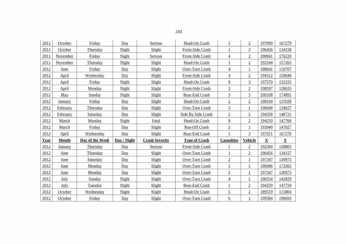
243

2011 October Friday Day Serious Head-On Crash 1 2 197009 167279


2011 November Friday Night Serious Front-Side Crash 4 2 200841 176220

2011 November Thursday Night Slight Head-On Crash 1 2 192544 157263

2012 June Friday Day Slight Over-Turn Crash 4 1 188641 110707


2012 April Friday Night Slight Head-On Crash 9 3 197570 132335

2012 April Monday Night Slight Front-Side Crash 3 2 198597 138635

2012 May Sunday Night Slight Rear-End Crash 3 3 200108 174891

2012 January Friday Day Slight Head-On Crash 2 2 198104 137028

2012 February Thursday Day Slight Over-Turn Crash 5 1 196640 134027

2012 February Saturday Day Slight Side By Side Crash 2 2 194358 148721

2012 March Monday Night Fatal Head-On Crash 8 2 194259 147760

2012 March Friday Day Slight Ran-Off Crash 2 1 193940 147027

2012 April Wednesday Day Slight Rear-End Crash 1 3 197011 167276


2012 January Thursday Day Serious Front-Side Crash 1 2 192304 158805


2012 June Saturday Day Slight Over-Turn Crash 2 1 197347 130975

2012 June Monday Day Slight Over-Turn Crash 1 1 199496 173565

2012 June Monday Day Slight Over-Turn Crash 2 1 197347 130975

2012 July Sunday Night Slight Over-Turn Crash 4 1 196554 142829

2012 July Tuesday Night Slight Rear-End Crash 1 2 194259 147759

2012 October Wednesday Night Slight Head-On Crash 5 2 189519 115804

2012 October Friday Day Slight Over-Turn Crash 6 1 199584 196693

244

2012 August Friday Day Slight Over-Turn Crash 1 1 197364 198070

2012 August Thursday Day Slight Head-On Crash 5 2 202239 182713


2012 September Tuesday Day Slight Ran-Off Crash 1 2 198635 171696

2012 October Thursday Night Slight Over-Turn Crash 1 1 192290 158710

2012 December Wednesday Night Serious Over-Turn Crash 4 1 197347 130975

2012 December Sunday Day Slight Skidding Crash 1 1 200664 193957

modeling relationship between geometric design … dwikat.pdfmohammed ghassan dwikat supervised dr....

Documents