Modeling of Integrated RF Passive Devices

Sharad Kapur and David E. Long

Integrand Software, Inc.

Berkeley Heights, NJ 07922 USA

http://www.integrandsoftware.com

Abstract—We describe the use of an electromagnetic (EM) sim-ulator for modeling integrated RF components and circuits. Mod-ern EM simulators are fast and accurate enough to provide goodmodels of such components. An important aspect of advancedIC processes is that the physical properties of wires (width,thickness, and resistance) vary depending on the surroundingwiring. We discuss how the EMX simulator [1] handles width-and spacing-dependent properties in the process description.Because the simulator handles mask-ready layout without theneed for manual simplification, it is feasible to simulate thousandsof possible designs and build scalable component models. Suchscalable models allow fast choices of optimal components thatmeet user-supplied specifications.

I. INTRODUCTION

Technology trends have made on-chip passive components

pervasive. Thick metals and high-resistivity substrates lead to

high-quality on-chip inductors, transformers, and baluns. For

example, integrated baluns can now be designed that have

insertion loss comparable to off-chip LTCC or ceramic baluns.

High-density interdigitated (MoM) capacitors are possible

because of fine feature sizes (0.1µm and below) and a large

number of interconnect layers (ten or more). IC processes also

offer tight tolerances, so variability from chip to chip is low.

And of course integration offers cost savings as well. Because

of their increased prevalence, fast and accurate modeling of

integrated passives is important. There are two main aspects

of this modeling:

1) EM simulation to evaluate candidate physical designs,

and possibly to refine the physical design.

2) Converting the EM simulation results into models that

can be used with higher level simulators, e.g., at the

circuit netlist level.

EM simulators fall into two broad categories: those based

on a differential formulation of Maxwell’s equations, and

those based on integral formulations. Examples of the former

include finite difference (both frequency- and time-domain)

and finite element simulators [2]. These offer flexibility, but

have the drawback that dielectrics, including a suitably large

amount of space surrounding the physical conductors, must

be discretized. This is because Maxwell’s equations must be

enforced wherever there is a non-trivial field. Integral (or

boundary element) formulations [3] are typically frequency-

domain, and are most appropriate when the enclosing dielectric

media is largely planar. They require discretization only of the

conductors, not the surrounding dielectrics. For IC passives,

planarity is an excellent approximation. Further, understanding

of how to efficiently implement boundary-element methods

has increased notably with the development of the Fast Mul-

tipole Method and related techniques [4]. Overall, frequency-

domain integral methods are usually the most efficient choice

when they are applicable, and hence are the most appropriate

for simulation of IC passives. We will concentrate on these

methods.

Converting frequency-domain simulation data into a form

suitable for a circuit simulator is a difficult problem in the

general case. However, in the more constrained domain of

modeling basic types of components, there are two basic

approaches. One is to use an optimizer to pick the parameters

of a user-specified circuit topology that is appropriate to the

device. While non-linear optimization in general is difficult, it

works reasonably well for this application. Approaches based

on pole-zero fitting are also workable. Care must be taken to

maintain passivity, but commercial tools are available, both

internally in some circuit simulators [5] or as stand-alone

applications [6]. Either optimization or pole-zero fitting are

appropriate for modeling individual passive components. Opti-

mization also offers the possibility of making scalable models.

A scalable model is parameterized by physical quantities. For

example, a scalable inductor model might be parameterized

by number of turns, diameter, wire width, and turn-to-turn

spacing. A scalable model captures the whole design space

of possible components. Having a scalable model makes it

possible to quickly synthesize an optimal design from a user-

supplied specification by searching the entire design space [7].

II. INTEGRAL FORMULATIONS FOR EM SIMULATION

Planar EM simulators based on integral formulations only

require discretization of the conductors, not the surrounding

dielectrics. All of the dielectric and substrate effects are

implicitly captured in the form of a Green’s function [8]. In the

frequency domain, the stimulus electric field Es at a point r

must match the field arising from ohmic losses, the vector

potential A and the scalar potential φ:

Es(r) =1

σJ(r) + jωA(r) +∇φ(r). (1)

The vector and scalar potentials are obtained by integrat-

ing over the conductors: A(r) =∫GA(r, r

′)J(r′) dr′, and

φ(r) =∫Gφ(r, r

′)ρ(r′)dr′. J is the current density, ρ is the

charge density, GA is the vector potential Green’s function,

and Gφ is the scalar potential Green’s function. For computer

simulation, this continuous equation is discretized by cutting

the conductors up into individual mesh elements, each with an

Custom Integrated Circuits Conference September, 2010

Fig. 1. 3D mesh of a stacked inductor

unknown charge and/or current. The integrals become finite

sums, and the problem can be expressed as a linear system.

Because of the integrals over conductor surfaces, integral

formulations give rise to dense systems of linear equations

after discretization. That is, a bit of current or charge in one

mesh element influences the potentials in all of the other mesh

elements. Dealing with this dense system of equations made

early simulators that used integral formulations comparable

in speed to those that used differential formulations, despite

the fact that the former required only a small number of

discretization elements. Later research in iterative methods for

the solution of linear systems [9] and in techniques for com-

pactly representing the linear systems that arise from integrals

involving potentials [4] dramatically increased the speed of in-

tegral formulation simulators. The techniques pioneered in first

generation fast field solvers from research institutions [10],

[11], [12], [13], [14] have been making their way into com-

mercial tools such as Agilent’s Momentum [15], Ansoft’s

Q3D Extractor [16], and Integrand Software’s EMX [1]. These

tools have added further improvements in speed and memory

efficiency. Additional refinements such as the use of fast direct

solvers are now appearing in academic contexts [17]. Since we

are familiar with the internals of EMX, we will discuss some

of the refinements that it uses [18].

In order to accurately model IC layouts, it is important

to simulate skin-effect and sidewall capacitances correctly.

Especially for MoM capacitors, a “2.5D” approximation using

thin conductors is insufficient. We use a volume integral

formulation that treats conductors and vias as true 3D objects,

as shown in figure 1.

EMX uses a special representation of the vector potential

interactions (normally the most computationally expensive

part of the simulation). The representation allows the vector

potential interactions to be computed with about the same cost

as the scalar interactions. The method depends on decom-

posing the currents into divergence-free and curl-free parts.

The divergence-free parts give the dominant contributions to

the vector potential, and these are captured exactly. The less-

important contributions of the curl-free part are approximated

in a way that is accurate to a bit better than 1%, which suffices

for IC problems.

Typical IC layouts are very regular. Beyond repeated in-

stances of a subcircuit or component, wires tend to be paths

of constant width, the distance between adjacent routing is

typically constant, and most routing is at 90 or 45 degree

angles. Simulators can use regularity to reduce both time and

memory requirements. Figure 2 shows repeated shapes in the

mesh of an inductor that can be exploited.

Fig. 2. Wire mesh with isomorphic shapes shaded

In practice, automation is just as important as simulation

speed and memory efficiency. If getting the layout into a

suitable form for the simulator requires significant hand edit-

ing, the human becomes the bottleneck. Most commercial EM

simulators have interfaces to the major IC design systems, and

they have methods for automating tasks such as via merging.

EMX automatically handles features typical of modern IC

layouts, such as via arrays, context-dependent contacts, and

metal fill and slotting.

III. PATTERN-DEPENDENT EFFECTS

One feature of advanced IC processes is that the physical

width, thickness, and resistance of a wire generally depends

on the surrounding wiring. Sometimes the variations are very

significant. Fabricated widths may vary by up to 50% from

the nominal (drawn) width, and sheet resistance can change

by a factor of two. Such variations are called pattern-dependent

effects. Because these effects can be so large, it is important

to account for them in simulation and modeling.

Some foundries now provide detailed information about

pattern dependencies. This information is usually in the form

of tabulated data, with the tables indexed by wire width and

spacing to adjacent wires. An example is TSMC’s interopera-

ble R(L)C extraction technology file format iRCX [19], [20].

This file format is now used for both static RLC extraction

and high frequency EM simulations.

The process description used by a simulator must include all

of the definitions of material properties (such as dielectrics and

conductivities) and all the cross-section dimensions (layer and

conductor thicknesses). EMX also allows the specification of

conductor properties to include width and spacing dependen-

cies. Internally, the the input (drawn) layout is automatically

modified in order to accurately model the fabricated structure.

Handling pattern-dependent effects requires:

• devising appropriate definitions of the local width and

spacing and developing efficient algorithms for comput-

ing these quantities; and

• manipulating the input geometry as a function of them.

We discuss these steps in the following two subsections.

Fig. 3. Exterior Voronoi diagram of some wiring

A. Computing Width and Spacing

For simple repetitive layout (e.g., multiple parallel wires)

width and spacing have intuitive meanings. However a simu-

lator must handle more complicated situations involving non-

uniform layout. We want definitions that match the intuitive

meanings in regular regions and that lend themselves to effi-

cient computation. For width and spacing, a natural geometric

data structure for representing local distances between objects

is the Voronoi diagram [21].

In the case of layout, the objects of interest are line segments

representing the edges of wires, and points where segments

join. Each segment and point has a region around it that

is closer to that object than to any other object. Following

this idea, the entire plane is partitioned into non-overlapping

regions, and this partitioning is the Voronoi diagram of the

segments and points. Note that part of the Voronoi diagram

lies within the wiring, and the rest lies outside. These two

parts are called the interior and exterior Voronoi diagrams.

A portion of a MoM capacitor layout and the associated

exterior Voronoi diagram is shown in figure 3. The shaded ar-

eas are the wires. Between the wires, there are some segments

which represent the boundaries of the Voronoi regions.1 Also

shown are some maximal inscribed circles. Each such circle

just touches three objects, and the circles cannot be made any

bigger while touching those objects.

The local spacing is taken from the diameter of the appro-

priate maximal inscribed circle that touches the segment and

the nearest other object(s). The local width is calculated in the

same way as the local spacing, except it is based on the interior

Voronoi diagram instead of the exterior one. Local width

and spacing can be calculated at key points throughout the

layout during the Voronoi diagram construction. Afterwards,

the values can be quickly interpolated at any desired location.

B. Mimicing Fabrication Effects

Typically the most significant fabrication effect is that

physical line width differs from the drawn width by a bias

amount which depends on the local width and spacing in the

1Technically, some of the boundaries are parts of parabolas, but computa-tionally it is easier to approximate these parts by segments.

TABLE IEXAMPLE VARIATION OF PHYSICAL WIDTH (MICRONS) AS A FUNCTION OF

DRAWN WIDTH AND SPACING

w\s 0.1000 0.1300 0.1500 0.2000 . . .

0.1000 0.1025 0.1125 0.1220 0.1470 . . .0.1300 0.1265 0.1285 0.1340 0.1525 . . .0.1500 0.1459 0.1459 0.1459 0.1599 . . .0.2000 0.1783 0.1783 0.1783 0.1783 . . .

. . . . . . . . . . . . . . . . . .

Fig. 4. Wires before (gray) and after (outline) bias

layout. The bias is obtained from a table provided by the

foundry. Table I shows an example of how the physical width

of a metal wire depends on the drawn width and spacing. For

example, a 0.1 µm drawn wire at a spacing of 0.2 µm will

physically expand to be 0.147 µm wide. That represents an

increase of almost 50% from the drawn width.

Interpolating in such a table produces a continuous function

for the bias as a function of drawn width and spacing. An

example of a layout before and after such a variable bias

operation is shown in figure 4. Note that the biased geometry

is not rectilinear when the width and spacing are not uniform.

Another significant effect is sheet resistance variation. After

calculating the local width and spacing and the biased geome-

try, the simulator can proceed with mesh generation as normal.

Then at each point in the mesh, the sheet resistance can be

calculated as a function of width and spacing. Each shape in

the mesh may be assigned a sheet resistance by averaging over

the area of the shape. An example of how resistance varies is

shown in table II. Note that the sheet resistance changes by

almost a factor of two as a function of width and spacing.

Figure 5 shows the variation in sheet resistance for a MoM

capacitor.

IV. EXAMPLES

We start with three examples that show the size of problems

that can be handled by a modern EM simulator. The ability

to simulate larger blocks containing multiple components al-

lows modeling more complicated structures where interactions

between components are also taken into account. All these

examples were run using EMX on a machine with eight

TABLE IIEXAMPLE VARIATION OF SHEET RESISTANCE (OHMS/SQUARE) AS A

FUNCTION OF DRAWN WIDTH AND SPACING

w\s 0.1000 0.1300 0.1500 0.2000 . . .

0.1000 0.1399 0.1220 0.1084 0.0839 . . .0.1300 0.1355 0.1316 0.1235 0.1034 . . .0.1500 0.1285 0.1275 0.1266 0.1116 . . .0.2000 0.1315 0.1305 0.1295 0.1286 . . .

. . . . . . . . . . . . . . . . . .

Fig. 5. Variation of sheet resistance in the mesh

2.5 GHz CPUs and 24 GB of memory. The speed-up for eight

CPUs compared to a single CPU depends on the characteristics

of the example and the number of ports, but it can be up to

six. In all of the examples, the input was mask-ready GDSII

layout. No hand-editing or simplification was done for any

of the examples. Wall-clock simulation times for even the

largest example was under two hours, fast enough that EM

simulation can be part of the design process instead of being

used only as a final step during “sign-off.” The maximum

memory requirement was under 10 GB.

A. IC Diplexer

Figure 6 shows an integrated diplexer in a 0.18 µm 5-layer

metal BiCMOS technology. The design contains resistors,

inductors, MiM capacitors, and probe pads. One main issue

for the designers was accounting for all of the couplings

Fig. 6. IC diplexer layout

0 2 4 6 8 10−50

−40

−30

−20

−10

0

GHz

dB

High Band

Measurement

EMX

0 2 4 6 8 10−50

−40

−30

−20

−10

0

GHz

dB

Low Band

Measurement

EMX

Fig. 7. IC diplexer measurements

Fig. 8. Integrated VCO layout

between inductors, and between inductors and interconnect.

Direct simulation of the whole structure ensured that no

significant interactions were missed. Comparisons of the high-

and low-band simulated and measured responses (figure 7)

show excellent agreement.

B. VCO

Figure 8 is an integrated VCO fabricated in a 6-layer

90 nm CMOS technology. It consists of an inductor and a

bank of 66 MiM capacitors that are switchable for tuning.

The inductor here is small, enough so that parasitic coupling

between the inductor and the interconnect and the details

of how the capacitors are hooked up must be considered.

Indeed, a block-by-block model failed to predict the VCO’s

behavior. Simulating the whole structure gave much more

accurate results. The simulated and measured tuning curves

are shown in figure 9.

C. IPD Diplexer

Figure 10 shows another diplexer built in an IPD (Integrated

Passive Device) technology. The design includes resistors,

inductors, and thin-film capacitors, plus the measurement pads.

10 20 30 40 50 609.5

10

10.5

11

11.5

12

Capacitor bank control

Outp

ut fr

equency (

GH

z)

MeasurementEMX

Fig. 9. VCO tuning characteristic measurements

Fig. 10. IPD diplexer layout

EM simulation was an integral part of this design. Starting

from the diplexer specification, an appropriate topology and

approximate component values were chosen. A preliminary

layout included the coils and ports where tuning capacitors

should connect, but the capacitor values were not yet fixed.

EM simulation produced a model that was used in a circuit

simulator and optimizer to pick appropriate capacitor values.

A final EM simulation confirmed that the device should

meet specifications, just as subsequent measurements proved.

Figure 11 compares simulations and measurements for the IPD

diplexer.

D. Pattern-Dependent Effects

Here we show the significance of pattern-dependent effects

by comparing simulations and measurements for MoM capac-

itors and stacked inductors. The technology is TSMC’s 65 nm

9-metal process, and the width and spacing dependencies are

given by an iRCX file.

The MoM capacitors vary in the number of metals used, the

widths of the metal fingers, and the spacings between fingers.

For this 65 nm technology the minimum width and minimum

spacing are both 0.1 µm. A mesh of one of the MoM capacitors

is shown in figure 12.

We did two sets of simulations: once with the wire proper-

ties fixed at their minimum-width, minimum-spacing values

(no iRCX), and once with the full iRCX information that

allowed EMX to mimic the fabricated layout. Figure III shows

the measured and simulated (low frequency) capacitance val-

0 2 4 6 8 10−50

−40

−30

−20

−10

0

GHz

dB

Low band

Meas

EMX

0 2 4 6 8 10−50

−40

−30

−20

−10

0

GHz

dB

High band

Meas

EMX

Fig. 11. IPD diplexer measurements

Fig. 12. Mesh of a MoM capacitor

ues for these MoM capacitors. For capacitors with minimum

width and minimum spacing, both simulations provided ex-

cellent agreement with measurements. However, for MOM36

with width 0.1 µm and spacing 0.16 µm there is a 0.2% error

when the iRCX file is used and a 13% error when it is not.

This ties in with the iRCX table in table I, which shows that

the bias is most significant for wires that have increased width

or spacing.

Figures 13 and 14 show the high-frequency characteristics

of the capacitors. For MOM06, with minimum width and

spacing, both iRCX and non-iRCX simulations agree well with

TABLE IIIMEASURED AND SIMULATED MOM CAPACITOR VALUES AT VARIOUS

WIDTHS AND SPACINGS OF FINGERS

cell meas iRCX no iRCXw, s µm pF pF %err pF %err

MOM060.1, 0.1 0.611 0.617 0.9 0.614 0.5

MOM670.16, 0.16 0.293 0.295 0.7 0.300 2.4

MOM270.1, 0.16 0.061 0.061 0.3 0.053 -13.1

MOM360.1, 0.16 0.682 0.680 -0.2 0.591 -13.3

0 5 10 150.5

1

1.5C

pF

0 5 10 150

100

200

300

400Q

0 5 10 150.5

1

1.5R

Oh

ms

GHz

Capacitor MOM06: w=0.1, s=0.1

0 5 10 1510

−3

10−2

10−1

Y

1/O

hm

s

GHz

Meas

EMX iRCX

EMX no iRCX

Fig. 13. Comparison of MoM capacitor simulation to measurement for acapacitor using minimum width and spacing

0 5 10 150.5

1

1.5C

pF

0 5 10 150

50

100Q

0 5 10 152

3

4

5R

Oh

ms

GHz

Capacitor MOM36: w=0.1, s=0.16

0 5 10 1510

−4

10−2

100

Y

1/O

hm

s

GHz

Meas

EMX iRCX

EMX no iRCX

Fig. 14. Comparison of MoM capacitor simulation to measurement for acapacitor using non-minimum width and spacing

measurements. However, for MOM36 the iRCX simulation has

excellent agreement while the and non-iRCX simulations has

a large discrepancy in C and Q.

We also simulated a stacked inductor. The inductor winds

from metal 5 through metal 9, and includes two thin metals as

well as the two thicker ones. The Q of the inductor depends

significantly on the resistance in the thin metals, and this

resistance varies as a function of metal width and the spacing

to nearby wires. This is exactly the effect seen in measurement

(figure 15). Again, the simulation taking width and spacing

dependence into account is significantly more accurate.

E. Balun Modeling and Synthesis

Now we discuss the production of a scalable model that is

suitable for synthesis of optimal components. As an example,

we consider on-chip baluns.

We start with a transformer layout generator whose inputs

are turns ratio, number of turns, trace width and coil diameter.

In the first step, we used EM simulator to characterize the

range of about 1000 possible transformer layouts. Thanks to

the simulators efficiency and automated layout handling, it

required only a day to cover the full possible design space:

wire width of 4 to 10µm, 2 through 5 turns, a turns ratio of

1:1 through 1:4, and a diameter of 50 to 400µm.

0 5 10 15 202

3

4

5

6L

nH

0 5 10 15 200

1

2

3

4Q

0 1 2 3 420

25

30R

Oh

ms

GHz

Stacked inductor

0 5 10 15 200

500

1000Z

GHz

Meas

EMX iRCX

EMX no IRCX

Fig. 15. Comparison of stacked inductor simulation to measurement

In the next step, we use optimization to create an accu-

rate scalable model parameterized by these same physical

design parameters. The topology for the scalable model was

derived from physical intuition and is shown in Figure 16.

The schematic shows a center-tapped pair of coils. Each coil

includes additional resistors and inductors for modeling skin-

effect. A combination of resistors and capacitors is used to

model the substrate.

P1 S1

S2P2

SCT

Fig. 16. Scalable model schematic

Each element in the model has a value that is a non-linear

function of the geometric parameters. The specific forms of

these functions are chosen based on physical intuition. For

example, the main series resistance in each coil is proportional

to the diameter and inversely proportional to the width. The

fitting coefficients within the functions are determined by a

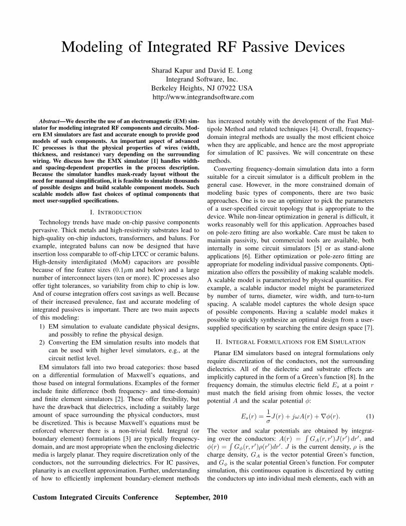
non-linear least squares optimizer. A playback was done of

the model compared to the individual EM simulations, and

the model was verified to match within a few percent for

derived quantities like inductance, k, Q, etc. For example, the

histogram of Figure 17 shows the percentage error in primary

inductance L1, secondary inductance L2, and k across the

design space. The optimizer took a few hours to build the

scalable model.

Given the scalable model of the transformer, simulation

0 1 2 3 40

100

200

300

400

500

600

700

800

900

L1 L2

k

Percent error

Nu

mb

er

of

insta

nce

s

Fig. 17. Comparison of model to simulations

of the performance of any particular balun (including the

tuning capacitors) takes only a fraction of a second. This

means that an exhaustive examination of the entire design

space can be done in under a minute. Constraints may be

placed on any combination of area, insertion loss, return loss

(matching), phase imbalance or amplitude imbalance. The

entire bandwidth of interest can be checked, and the desired

input and output impedances can also be specified during the

search. While the EM simulation and the construction of the

scalable model is time-consuming, the actual synthesis of any

given balun is very quick. Such scalable models derived from

EM simulations and linked with optimal synthesis capabilities

are now provided by some foundries as part of their design

kits for components like inductors, capacitors, transformers,

and baluns.

This method was used to design four baluns for common

applications: 802.11A, 802.11B, DCS and GSM. A standard

single-ended impedance of 50Ω and a differential output

impedance of 200Ω were chosen for demonstration. The

baluns were fabricated in UMC’s 90nm, 9-level IC process.

3µm copper was used for the coil, and thinner metals were

stacked to form the underpasses. Tuning MIM capacitors of

2fF/µm2 were used. In all the layouts, coil area dominated

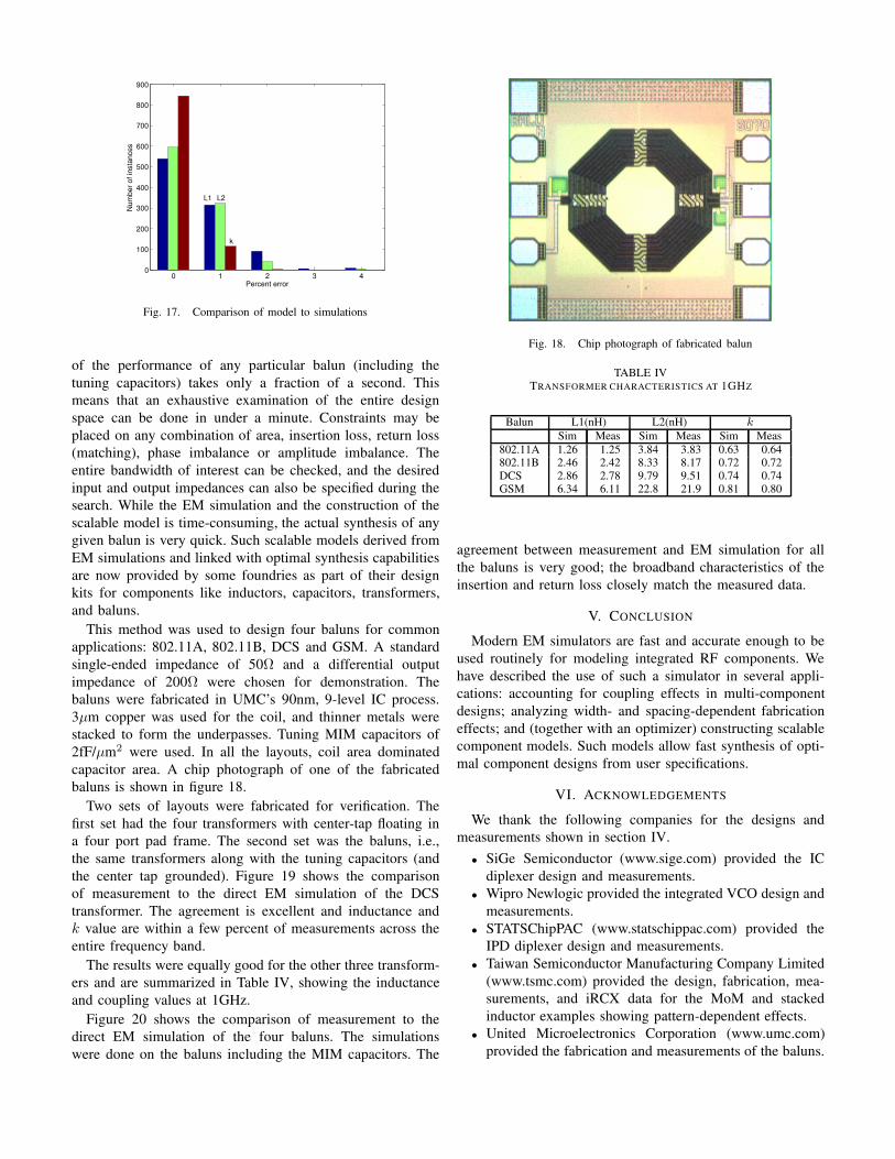
capacitor area. A chip photograph of one of the fabricated

baluns is shown in figure 18.

Two sets of layouts were fabricated for verification. The

first set had the four transformers with center-tap floating in

a four port pad frame. The second set was the baluns, i.e.,

the same transformers along with the tuning capacitors (and

the center tap grounded). Figure 19 shows the comparison

of measurement to the direct EM simulation of the DCS

transformer. The agreement is excellent and inductance and

k value are within a few percent of measurements across the

entire frequency band.

The results were equally good for the other three transform-

ers and are summarized in Table IV, showing the inductance

and coupling values at 1GHz.

Figure 20 shows the comparison of measurement to the

direct EM simulation of the four baluns. The simulations

were done on the baluns including the MIM capacitors. The

Fig. 18. Chip photograph of fabricated balun

TABLE IVTRANSFORMER CHARACTERISTICS AT 1GHZ

Balun L1(nH) L2(nH) k

Sim Meas Sim Meas Sim Meas

802.11A 1.26 1.25 3.84 3.83 0.63 0.64802.11B 2.46 2.42 8.33 8.17 0.72 0.72DCS 2.86 2.78 9.79 9.51 0.74 0.74GSM 6.34 6.11 22.8 21.9 0.81 0.80

agreement between measurement and EM simulation for all

the baluns is very good; the broadband characteristics of the

insertion and return loss closely match the measured data.

V. CONCLUSION

Modern EM simulators are fast and accurate enough to be

used routinely for modeling integrated RF components. We

have described the use of such a simulator in several appli-

cations: accounting for coupling effects in multi-component

designs; analyzing width- and spacing-dependent fabrication

effects; and (together with an optimizer) constructing scalable

component models. Such models allow fast synthesis of opti-

mal component designs from user specifications.

VI. ACKNOWLEDGEMENTS

We thank the following companies for the designs and

measurements shown in section IV.

• SiGe Semiconductor (www.sige.com) provided the IC

diplexer design and measurements.

• Wipro Newlogic provided the integrated VCO design and

measurements.

• STATSChipPAC (www.statschippac.com) provided the

IPD diplexer design and measurements.

• Taiwan Semiconductor Manufacturing Company Limited

(www.tsmc.com) provided the design, fabrication, mea-

surements, and iRCX data for the MoM and stacked

inductor examples showing pattern-dependent effects.

• United Microelectronics Corporation (www.umc.com)

provided the fabrication and measurements of the baluns.

0 1 2 3 4−60

−40

−20

0

20

40

60

GhZ

nH

L1 and L2

L1

L2

0 1 2 3 4−1

−0.5

0

0.5

1

1.5

GhZ

k

k=L12/sqrt(L1*L2)

0 1 2 3 4−10

−5

0

5

10

GhZ

Q1 and Q2

Q1

Q2

EMX

Meas

Fig. 19. Inductance, k, and Q of the DCS transformer: simulation vs measurement

2 4 6 8 10−35

−30

−25

−20

−15

−10

−5

GHz

802.11A

dB

RL

IL

2 4 6 8−35

−30

−25

−20

−15

−10

−5

GHz

802.11B

1 2 3 4 5 6

−35

−30

−25

−20

−15

−10

−5

GHz

DCS

1 2 3 4

−35

−30

−25

−20

−15

−10

−5

GHz

GSM

EMX IL

EMX RL

Meas IL

Meas RL

Fig. 20. Insertion loss (IL) and return loss (RL) of baluns: simulation vs measurement

REFERENCES

[1] EMX User’s Manual, Integrand Software, Inc., 2010.[2] R. Garg, Analytical and Computational Methods in Electromagnetics.

Artech House, 2008.[3] J. J. H. Wang, Generalized Moment Methods in Electromagnetics.

Wiley, 1991.[4] L. Greengard and V. Rokhlin, “A new version of the fast multipole

method for the Laplace equation in three dimensions,” Acta Numerica,vol. 6, pp. 229–269, 1997.

[5] Spectre Circuit Simulator User Guide, Cadence Design Systems, Inc.,2009.

[6] Sigrity, “Broadband SPICE,” http://www.sigrity.com.[7] S. Kapur, D. E. Long, R. C. Frye, Y.-C. Chen, M.-H. Cho, H.-W. Chang,

J.-H. Ou, and B. Hung, “Synthesis of optimal on-chip baluns,” in Proc.

Custom Integrated Circuits Conf., 2007, pp. 507–510.[8] W. C. Chew, Waves and Fields in Inhomogeneous Media. IEEE Press,

1995.[9] R. Barrett et al., Templates for the Solution of Linear Systems. SIAM,

1994.[10] S. Kapur and D. E. Long, “Large-scale capacitance calculation,” in Proc.

37th Design Automation Conf., Jun. 2000, pp. 744–749.[11] S. Kapur, D. E. Long, and J. Zhao, “Efficient full-wave simulation in

layered, lossy media,” in Proc. Custom Integrated Circuits Conf., May1998, pp. 211–214.

[12] K. Nabors and J. K. White, “FastCap: A multipole accelerated 3-Dcapacitance extraction program,” IEEE Trans. on CAD, vol. 10, no. 11,pp. 1447–1459, Nov. 1991.

[13] J. R. Phillips and J. K. White, “A precorrected-FFT method for elec-trostatic analysis of complicated 3-D structures,” IEEE Trans. on CAD,vol. 16, no. 10, pp. 1059–1072, Oct. 1997.

[14] Z. Zhu, B. Song, and J. K. White, “Algorithms in FastImp: A fast andwideband impedance extraction program for complicated 3-D geome-tries,” in Proc. 40th Design Automation Conf., 2003, pp. 712–717.

[15] Momentum – ADS 2009, Agilent Technologies, 2009,http://edocs.soco.agilent.com/display/ads2009/Momentum.

[16] “Q3D extractor,” Ansys, Inc., 2009, http://www.ansoft.com/products/si/q3d extractor.

[17] W. Chai, D. Jiao, and C.-K. Koh, “A direct integral-equation solverof linear complexity for large-scale 3d capacitance and impedanceextraction,” in Proc. 46th Design Automation Conf., 2009, pp. 752–757.

[18] S. Kapur and D. E. Long, “Large-scale full-wave simulation,” in Proc.

41st Design Automation Conf., 2004, pp. 806–809.[19] iRCX Unified Technology File Format Usage, TSMC, 2008, verion 1.4.[20] T-N65-CL-SP-009-I1 65nm iRCX file at http://online.tsmc.com, TSMC,

2008.[21] T. Imai, “A topology-oriented algorithm for the Voronoi diagram of poly-

gons,” in Proc. 8th Canadian Conference on Computational Geometry,1996, pp. 107–112.