■"■■^■■■"^^W" ■ I' •> " ■ " ■ll"'1 '-- i in i^^^mmmtu i n n > ■mwuppnttPMnqn^H*«

CO

00 CO

Final Quarterly Technical Report

MODELING OF TRANSIONOSPMERIC RADIO PROPAGATION

By: E. J. FREMOUW C. L. RINO

Prepared for:

ROME AIR DEVELOPMENT CENTER GRIFFISS AIR FORCE BASE ROME, NcW YORK 13441

Attentior; MR. RICHARD A. SCHNEIBLE (OCSE)

CONTRACT F30602-74-C-0279

Sponsored by

DEFENSE ADVANCED RESEARCH PROJECTS AGENCY ARPA ORDER NO. 2777

/ A

STANFORD RESEARCH INSTITUTE Menlo Park, California 94025 • U.S.A.

-j-3 - —■■-— ■- ■■, - ■- - - ■ ■ --■ —- - ■■■ -■■-■■--•-

mmm^m^^m^^m " mmmmmmmmmmmrwm^mm

tIT™0™5***™ .NST.TUTE U.S.A.

(D ^ Fmel Quanerly TK^,, „„^ /4 - fc -/y /nai, -7 «T

MODELING OF JRANSIONOSPHKir RADIO PROPAGATION RADI

^ja By: E. J. TREMOUW

C L. RINO

(£>. Augm IB?5

Prepared for:

ROME A|R DCVPLOPMENT CENTER GRIFFISS AIR FORCE BASE ROME, NEW YORK 13441

Attent,0n: {0RCSER),CHARD A- ICHNe,B«

(315) 330-3085

Sponsored by:

I X

^ESsoNDV

BAoNuCuDvA

RpTRCH PR0JECTS A-«V ARLINGTON, VIRGINIA 22209

Attention: MR. JAMES C. GOODWIN

STRATEGIC TECHNOLOGY OFFICE

SRI Project 3416

CONTRAC^ F30602-74-C-0279 /W^ ^ ' - Effective ohn* Contract:' r^ayTg^^ "l Ä^T Contract Expiration Date: 14 May 1975 ^ 9 Amount of Contract: $99 542 Principal Investigator: E. Fremouw

(415) 326-6200, Ext. 2596 ARPA Order No. 2777 Program Code No. 44E20

Copy H0, KsCy

33'X 'TO 0

■ -...v^.,-...—^_.—.. -■_. —^■■. - ..,

[

- - - - . -

pp^xv 11 m. ■ um^mtmmm mmmmmmmimmu i mipimBii m^^m^mmmmmmm'^^mm^mmmmmmim UM--—,

CONTENTS

LIST OF ILLUSTRATIONS 111

LIST OF TABLES lv

I REPORT SUMMARY 1

II SCATTERING THEORY EMPLOYED 3

III SCINTILLATION MORPHOLOGY MODELED 23

IV THE CHANNEL-MODEL CODES

V CONCLUSION 41

REFERENCES 47

ii

^^u|Mt||^^^^HMa^^MM^^|^^^^^^^^^M| - . — - HMMiMMiHi HMa

mmm^m'" mmm^^mmmmm

ILLUSTRATIONS

mm**

Phasor Diagrani for Consideration of First-Order

Signal Statistics, Showing Elliptical Contour of Equal

Probability Predicted by the Gaussian-Statistics

Hypothesis ^

Scintillation Index S, as a Function of Elongation and

Orientation of the Equal-Probability Ellipse, for Four

Values of Ionospheric Scattering Coefficient, R0 8

Comparison of Algebraic Approximation (Eq. 20) to Values

of the Integral in Eq. (17) 16

Scatter Plot Showing Degree of Correlation Between

Auroral Electroject Index, AE, and Planetary hagnctic

Index, Kp 27

Comparison of Model Calculation (solid curve) with

Diurnal Variation of 136-MHz Intensity-Scintillation

Index Observed (Xs) by Koster (1968) in the Equatorial

Region 29

Comparison of Model Calculation (solid curve) with the

Seasona1. Variation of 136-MHz Intensity-Scintillation

Index ■ bserved (Xs) by Koster (1968) in the Equatorial

Region 29

Comparison of Model Calculation (solid curve) with Diurnal

Variation of 40-MHz Intensity-Scintillation Index Observed

(Xs) by Preddey, Mawdsley, and Ireland (1969) in the Mid-

Latitude Region 30

Comparison of Model Calculations (solid curves) with the

Latitudinal Variation of 400-MHz Intensity-Scintillation

Index, for Three States of Geomagnetic Disturbance,

Observed (symbols) by Evans (1973) Near the Subauroral

Scintillation Boundary 30

Comparison of Calculated (smooth curve) Probability

Density Function for Amplitude with Observations

(histogram) of ATS-5 Transmission at 137 MHz, Made by

Aarons (private communication, 1974) Through the Mid-

Latitude Ionosphere from Near Boston 31

iii

....- ■ . ^^^^^^^^^^^ i^M

mmm^Kmmmmi^m^wmm^'i*' «HIM rw^pwil iniaj i

II

10

11

12

13

14

15

16

17

Comparison of Calculated (smooth curve) Cumulative

Probability Function (cpi) for Intensity (or for

amplitude) with Observations (histogram) for Case in

Figure 9 31

Calculated Probability Density Function for Phase for

the Case in Figures 9 and 10 32

Simplified Flow Chart of PROGRAM RFMOD 34

Sample Input Cards for PROGRAM RFMOD 35

Example of Output from Available Version of PROGRAM RFMOD . . 39

Example of Amplitude pdf Output from Available Version

of PROGRAM DIST 42

Example of cdf Output from Available Version of

PROGRAM DIST 43

Example of Phase pdf Output from Available Version

of PROGRAM DIST 44

TABLES

1 Routines in PROGRAM RFMOD 33

2 Data-Card Variables 36

3 Contents of Changing-Paiameter(s) Card 38

4 Routines in PROGRAM DIST 40

iv

■ ■-_..- _. - . ■_ ^-

immmmm ^^^m^mi^mmm^m 1 i umimii^^mmmmmmmmmm^mmmm^i^mmrgMmi I«I i i BWPil|IIIWIP«lll'"IIWI»»WWPWP^,"""">"i™

I . REPORT SUMMARY

This is the final quarterly technical report on a one-year contract

to extend and improve an existing empirical model for worldwide behavior

of ionospheii-cally imposed radio-wave sci|ntillation. The objectives of

the project were (1) to improve the accuracy of model-based calculations

of the intersity-sclntillation index and (2) to develop a capability for

full description (from the point of view of engineering t.-plications) of

the first-order, complex-signal statistics that characterize tbn trans-

ionospheric radio communication channel. A follow-on project has been

initiated to extend the channel model to include second-order signal

stauistics in the temporal, spatial, and spectral domains. The first

priority in the follow-on work • ill be to calculate the fluctuation

spectra of relevant signal parameters. In addition, it is intended to

extend validity of the model into the multiple-scatter regime

^ The stated objectives of the just-completed project were accomplished

by starting with the scintillation mod 1 developed by Fremouw and Rino

(1973) , adding a geomagnetic-activity dependence for the behavior of

scintillation-producing ionospheric irregularities, and substituting a

more accurate and general scattering theory for that of Briggs and Parkin

(1963) used in the earlier model. The results of these efforts have

been implemented in two computer programs. The first, entitled RFMOD,

contains the main elements of the scattering theory, the morphological

model for ionospheric irregularity strength and other parameters, and

subroutines for calculating the geometry and other relevant quantities

from user-specified inputs. The main outputs of RFMOD are the intensity-

scintillation index SA, which is the fractional rms fluctuation in re-

ceived signal intensity (Briggs and Parkin, 1963), and an analogous phase

scintillation index $rms (labled PRMS), which is the rms fluctuation of

phase.

■ ■■■

..„„. . . .^. . .

^ —' — "■'"

:

Three related first-order, signal-statistical parameters also are

output from RFMOD, to be used as inputs to the second program, called

DIST. The latter program permits calculation of the first-order dis-

tribution functions of amplitude and phase for selected values of S4

and/or $rms. There are three types of output from DIST: values of the

probability density functions (pdf) for amplitude and for phase, and

values of the cumulative probability function (cpf) for intensity (or,

equivalently, for amplitude since the argument is output in dB relative

to the undisturbed level). The cpf output constitutes estimation of

fade margin required to combat amplitude scintillation.

RFMOD and DIST represent interim versions of evolving transiono-

spheric communication-channel codes. As stated above, capabilities

will be added for calculating second-order statistics. More relevant

in the near term is that there has been no direct testing of calculations

relating to phase scintillation. As was recognized at the outset of the

project, data are not available at present that are directly relevant

to testing phase statistics unambiguously. Useful data are expected

from forthcoming observations of milClfrequency coherent satellite

beacons, and such tests will be made. The forthcoming data may also

result in model changes that will further alter the calculated results

for amplitude scintillation, because testing to date has still necessarily

relied on some observations reported in terms of a partly subjective

scintillation index. In addition, while the assumption of weak, single

scatter contained in the Briggs-and-Parkin theory has been partially

removed, a more complete correction for multiple scatter effects has yet

to be incorporated.

This report represents a summary of the work performed during the

past year and is inteded as a status report on the evolving SRI/ARPA

channel model. Section II describes the scattering theory employed and

■

* liilt*m^mmmm riduHiiiBMiMriMMeeHi

•' """' «"■■li.llll

compares some of its salient poit.ts with those of other theories. That

section includes some material reported in earlier quarterly reports,

for the sake of presenting a coherent discussion under one cover, but

there is no attempt to describe the theoretical development in chrono-

logical detail. Section III contains a brief review of the known mor-

phology of scintillation-producing ionospheric irregularities as modeled

in RFMOD. A functional description of the programs RFMOD and DIST is

presented in Section IV, along with instructions for their use. Finally,

in Section V, we present our conclusions on the utility and limitations

of the channel model in its präsent form and some prospects for further

improvement.

II SCATTERING THEORY EMPLOYED

The basic approach to modeling the transionospheric communication

channel is to treat the channel as a time-and-space-varying linear filter

linking the transmitting and receiving antennas of a communication sys-

tem. Slowly varying effects (on a time scale of many minutes or hours),

such as group delay, polarization change, and dispersion of signals

propagating through the smooth ionosphere, can be described by well-

known deterministic methods and are not included in this work. What is

treated are the relatively rapid and random variations (on a time scale

of fractions of a second to a minute or so) In signal parameters that

arise due to scattering by irregularities in ionospheric electron density

and that are referred to as scintillations. Because the channel can be

treated as a linear filter, standard Fourier techniques can be used to

apply the results to modulated signals if a sufficiently general descrip-

tion is provided of the signal statistics resulting when a continuous

(CW) is passed through the channel (Fremouw, 1969). In this section,

we. discuss the first-order statistics of this basic signal.

mm^äämtatto^äällMmtUKtot ■JBMUMMMlMlHMtal .■..J--..-J—t^-^.-.-. .. ■■- .^' .* ;——

rmmmmmmmmm^fmmmi^^mm^nmmmm'' • • "'"■•"■"'.' immmmmmmmmmm.mfM m 1 mmn^rmrmmvi'^^m^mm

Any LW Fignal can be represented by a vector on the complex plane,

such as the phasor E in Figure 1. In this figure, E = ^E^ + IE j is meant

to represent the randomly time-varying complex amplitude of the signal

output from an antenna terminal. In describing the first-order, complex-

signal statistics of E, we are assessing the probability that the tip of

the phasor lies within an elemental area on the complex plain. To begin,

we write E as the resultant of its long-term mean (E) and a zero-mean,

randomly varying component E . We choose to reference all phases to

that of <E>, which is the same as the phase that E would have in the

I

<E> = TJ Re AXIS

LA-3416-12

FIGURE 1 PHASOR DIAGRAM FOR CONSIDERATION OF FIRST-ORDER SIGNAL STATISTICS, SHOWING ELLIPTICAL CONTOUR OF EQUAL PROBABILITY PREDICTED BY THE GAUSSIAN- STATISTICS HYPOTHESIS

absence of channel-imposed perturbations because we have excluded slow

channel variations from the model. (Thus (E ) = 0, and (E > 8 T\ ■ y x

(E>.) The magnitude of (E) (= Tfl is less than the amplitude of the un-

disturbed signal, however, because some of the transmitted energy has been

scattered into the randomly varying component E .

4

^MMiMMai^^^^^H dMA^MMi

^^^^""""^■""•««^^^^""i i ...i i ii. i «MI ii ,1 mm^^^m^mmmmm^^^^^^m^m^mm

To proceed with the analysts, it is convenient to break E^ into

its own real and imaginary components, S and S , respectively. The x y

convenience stems in part from the fact that the variances of S^ and 0 0 £ *

S a and a , respectively, and their covariance 0 can be calculated y' x y xy

in terms of ionospheric parameters. These are useful calculations to 2 2

perform because, at the very least, the sum of a^ and c^ represents the

powar contained in the scattered signal, which we shall denote as 1^.

That is,

R = <E E*) = c + a . (1) o s s x y

We shall normalize all our calculations to unity total received power,

so R will represent the fraction of flux scattered--!.e., the forward- o ttering coefficient of the ionosphere. A complex quantity analogous

o sea

to the real R that it is useful is the following (Rino and Fremouw, o

1973a):

B = ^ E > = (o2 - o2) + 2i a . (2) oss x y xy

If it should be that the quadrature components, E and E , are

jointly Gaussian random variables, the utility of the three variances

defined above--or alternatively of R and B^-would be very great. Indeed

in this instance the first-order statistics of the received signal E are

totally defined by either of these sets of three parameters (i.e., the

three real variances or the real R and the real and imaginary parts of

B ). Most scintillation observations have been only in terms of the o

magnitude of E (i.e., amplitude or intensity scintillation) because a

sufficiently stable phase reference for measuring its complex value has

seldom been available under scintillation conditions. Thus, there has

been no direct determination of the complex-signal statistics. (This

. ..—^:..—^.-.f-^-L . iiafna^ji f.^^g^^^^^^^^^^^^^^Mgg^^^/a^^jM^jäA^^^^^^^äggmmmaiä^^t/t

1 ' ' ' • I" wwnm^mm» 1 J '

data deficiency should be remedied within the next year by means of

careful measurements of signals from the VHF-UHF coherent beacons on

ATS-6 and the Transit satellites and, under a wider range of ionospheric

conditions, by means of observations of the forthcoming DNA-002 multi-

frequency beacon.)

The Gaussian-statistics hypothesis (i.e., that the quadrature com-

ponents are jointly Gaussian variates) has been tested indirectly, however,

by means of amplitude-scintillation data. Rino, Livingston, and Whitney

(1975) assessed this hypothesis and the competing one of log-normal

statistics (according to which the phase and the logarithm of amplitude

are jointly Gaussian variates) by performing chi-square, goodness-of-fit

tests of amplitude histograms to amplitude pdfs calculated from the two

hypotheses. Good fits were found in general for both hypotheses, which

tend toward identical pdfs as the scintillation index de-.reases, but

the Gaussian hypothesis yielded better fits to 11 out of the 12 data

sets tested. This result is fortunate because it permits presentation

of scintillation calculations in a form that will be rather familiar to

communications engineers. In the remainder of this report, we proceed

on the basis of the Gaussian signal-statistics hypothesis.

For Gaussian signal statistics, a contour of equal probability for

the tip of the E-phascr on the complex plane is an ellipse (Beckman and

Spizzichino, 1963), such as the one in Figure 1. The analytical task of

first-order, signal-statistical channel modeling, then, is to relate the

parameters of such an ellipse to parameters of the channel (scattering

irregularities in the ionosphere in the present case). The probability

ellipse is characterized by its size, eccentricity, and orientation on the

complex plane. Clearly. Ro (being the fraction of flux scattered) dic-

tates the size of the ellipse. The eccentricity is dictated jointly by

R and the magnitude of B^ and the orientation is controlled by the phase

angle of B . Spec:fieaiy, the axial ratio of the probability ellipse is

given by

-■' ■LJW' JJ^-—.:-^....^....—..—^.^-J.» ■ ■ - - - - - -~ — ' - -- ^ .^„, .__ ..... .. .

•""""-•"'• '" " !«■■ "iMiiipiii utmnitmm ""■■""""

1 +

1/2

(3)

and its orientation angle, 6 (shown on Figure 1), is given by

1 TT

(4)

It will be recognized from Eqs. (1) through (4) and the accompanying

discussion that there are several sets of three parameters that can be

used to describe the first-order, complex-signal statistics. For reasons

of convenience, which will become clear in the ensuing discussion, we

choose to work with the parameters R , |B |/R , and 6, As an example of o o o

the relationship of these three parameters to a quantity of direct

applications interest, we have plotted the intensity-scintillation index

S in Figure 2 from the following formula derived by Nakagami (1960): 4

S, = 2R (1 - R ) 4 o o

L^-cos 26 U R2

R 10 1 + (5)

We note that in Briggs' and Parkin's theory, S is calculated

approximately as

cos 26 (6)

I ' .-■..-:- ^..^^^.^l^

—'■■ ■"—' ——^

1.2

1.0

0.8

0.6

Ro = 0.4 \

Ro - 0.36

-0.7 A s ^ ̂

^

1

— •^,

FIGURE 2 SCINTILLATION INDEX S4 AS A FUr.CTION OF ELONGATION AND OP ENTATION OF THE EQUAL-PROBABILITY ELLIPSE, FOR FOUR VALUES OF IONOSPHERIC SCATTERING COEFFICIENT, R0

The following three relationships arise from Eqs. (1) and (2)

2 Ro cos (26) (7)

R [ r. 2 o

0 = y

^ll + ^^cos (26) 2 L Ro (8)

uaMtfiaitiaHair ■'■'- ■■-

^

F"»^Wi^^^W^^"^» mm~~mmmm <ir^—*mmmim

xy sin (2&) (9)

Th us, Eq. (6) contains o .ly the contribution of the in-phase scattered

nt S to S . It arises from equating fluctuations in E to compone... x 4

fluctuations in the real amplitude A and is accurate only for very weak

scatter [i.e., when the higher-order R terms in Eq. (5) are negligible].

A significant improvement in th« present scintillation model is retention

of all terms in Eq. (5), which accounts for the contribution of fluctua-

tions in the phase-ouadrature component E (=S ) to amplitude scintilla-

tion (as well as for :he influence of the correlation between S and S ). x y

Other differences between the old scattering theory and the new

arise in the manner of calculating R and B . The basic approach used

in the present work is that described by Rino and Fremouw (1973b), in

which the scattering geometry is treated quite rigorously. Briggs and

Parkin simplified the geometry by assuming that the ionospheric scattering

layer effectively can be tilted from the horizontal so that its boundaries

are always normal to the incident radio-wave propagation vector. This

approximation breaks down for large zenith angles but it avoids a great

deal of complication in derivation of the scattering equations. Some of

this complication was avoided by Rino and Fremouw (1973b) by assuming

zero correlation in electron-density fluctuation along the vertical, which

has negligible effect on the scattering equations for nearly vertical

incidence. Again, however, the effect of the assumption becomes un-

acceptable as the incidence angle increases.

During the last quarter of this contract, the theory was recast to

include the scattering effect of structure in all three dimensions of

the ionosphere. An outline of the derivation is given here, together

with the resulting equations for describing first-order signal statistics,

■ - -- ■HHWaMiaiiHViiianmUi «MAMMMMMateMadM

rl mir^mmmmmm^^^ «■liaHW.IIIipjIIIIIBIIIII 11 "I " i"ii«" "Hii .11

which are valid over a greater range of incidence angles than their

counterparts in Quarterly Technical Reports 1 and 2.

The scattering coefficient R represents a special case of the

spatial autocorrelation function of the scattered signal, which is

defined as

R(P) = <E (r) E (r + P)> (10)

namely, the case in which the spatial lag parameter P is zero. A similar

definition, calculated without taking the complex conjugate, can be made

of a quantity B(p), which reduces B in the same special case (i.e.,

zero lag). The approach to evaluating R(P) and B(p) is to express Es

as the scattered field calculated by means of the first Born approxi-

mation, with the scattering medium rer^esented by a spatial spectrum of

ionospheric structure. The field is calculated by integrating the

contribution from different heights within the scattering layer, con-

sidering the diffraction effects arising in propagation to the observing

plane but ignoring effects of multiple scatter. When the complex field

is multiplied by its complex conjugate, the effects cancel.

The result is that R(P) can be expressed as the two-dimensional

Fourier transform of a height-smeared version of the ionosphere's spatial

■pactrun and B(P) can be expressed as the transform of that spectrum

times a propagation factor. Setting the lag parameter to zero is tanta-

mount to integrating over the spectra in the observing plane (as opposed

to calculating the Fourier transforms), with R being an integral over

the scattered field's angular power spectrum and B being an integral

over a complex spectrum that incorporates diffraction effects.

Irobably more important for first-order statistics than the approach

to deriving R and B is the form of the spatial spectrum used in o o

10

± ^^^^^^^^^^^ ------ - -

r mmmimmm!mim*mmmmmmmmmmm*i ■■""■'"" II«IJ*I in

their calculation. In evaluating R and the second factor in Eq. (6), o

Briggs and Parkin assumed a Gaussian-shaped spatial spectrum for the

ionosphere. While convenient because of its Fourier-transfomation

characteristics, a Gaussian spectrum does not appear to represent

ionospheric structure very realistically (Rufenach, 1972; Dyson et al.,

1974) .

A better description is afforded by a power law with a low-frequency

cutoff. When normalized so that its three-dimensional integral is unity 2

times the spatial variance ((AN) ) of electron density, such a spectrum

3 2

[units of (electrons/m ) per unit three-dimensional spatial frequency,

KJ may be written as

3C(tC) = 8rr 3/2 r(v + 1/2) Q3a ((AN)2)

r<v-1) ii + te^2! - -21v + 1/2 (il)

where V is the spectral index defining the power law, a is scale-size

parameter controlling the low-frequency cutoff, a is the ratio of

irregularity scale size along the geomagnetic field to that across the

field, and the three dimensional shape and orientation :>£ the irregulari-

ties (Budden, 1965), are described by

S2(K) = AUO K2 + K2 + B(^2 - 2C(^)K < x y z x z

(12)

where

A(« =

2 2 a + C (t)

»(♦) (13)

2 2 2 B(i|i) = cos 'i + a sin (14)

n

m^t^^^^^m ^.-^M^lac^, . ^..M.

mmm —— imn^nmmnm mmmm* ■w«» ^im'f^mt^mm^mmmfmmm^'l'-'w»" m

c(t) ■ (i - O cos ♦ sin t

and '; = the magnetic dip.

(15)

The coordinate system used is such that K is directed to the geomagnetic

north K to the geomagnetic east, and K downward. ' y z

Using the above spectrum, one obtains the following expression for

R

R =2^r2X2T>- ^ ^JÜ^LW) .

o e r(v - 1) ,, .( r (16)

where r = classical electron radius, e

\ = observing wavelength,

L = thickness of scattering layer,

A' = mLo' + D],

C' = 1/2[D' - D],

2 D' = i + B(\II + 90°) + 2C(t) tan ü cos 0 + B('i) tan 9,

and

D = /LD' - 2(1 + sin2 e)]Z + (B')2 ,

B' = B(^) tan2 6 sin 2C5 + 2C(t) tan 6 sin 0,

9 = incidence angle on scattering layer,

0 = propagation azimuth relative to geomagnetic north at

height of scattering layer.

Eq. (16) was obtained by integrating analytically over the angular

power spectrum of the scattered wave arriving at the observing plane,

as described above. The integral over the complex spectrum associated

with B cannot be performed analytically. However, the real and imaginary o

integrals involved have been solved numerically for a large range of

12

SHM^Ut^ ..■_J...^..^._.. -_ ...... ... - . . . . ,.... .-^ ■>.-.. . .—^...-■.■^. -.,—— -— -• -■--■■-"■■■-"■ ■ — - - --- - ■ - m.

r ^mmmmm mm -**m~<mmmmiimmß*m* mi^mmmmmmmm*™^*™**!.!" mm. i ■■■

geometrical situations described by the parameters «. *. 6, and 0. Study

of the numerical results has led to approximations suitable for Implemen-

tation In an operating computer code such as RFMOD.

Simplifications have been found by converting the real and Imaginary

integrals to the magnitude and phase angle of Bo and then to the quantities

|B l/R and 6 Uhe latter via Eq. (4)j. The simplification arises from

an^molrlcally noted approximate relationship between the latter two

quantities, as descrlbad In detail In Quarterly Technical Reports 1 and 2.

It permits approximate description of the complete first-order, complex-

signal statistics from solution of the real integral alone. What is

actually calculated is a^, which is related to RelB^ by Eq. (7).

Two approximations are involved in formulating this part of the

problem. The first-neglect of a diffraction effect related to layer

thickness-appears numerically to be valid essentially anywhere outside

the scattering layer. The second holds so long as the spectrum of

irregularities contributing to Ex fluctuations is cut off at the low-

frequency end by diffraction effects rather than by an Inherent cutoff

of the ionospheric spatial spectrum. Both in-situ (Dyson et al., 1974)

and scintillation observations (Rufenach, 1572; Rlno, Livingston, and

Whitney, 1975) support this view for all frequencies of interest. We

have, therefore, ^oceeded on the basis of this "near-zone" approximation,

but we have Incorporated a test In RFHOD to safeguard against violation

of the assumption underlying it. On the basis of these two approximations,

2 one may write a /R as follows:

x = 2(v - 1/2) V A ' AZ sec

i vl 2 (C ) VA" a

1/2

13

L. in MBiMin^^iaMh^M »m^^^^M^^mmM ■ -- -^ ...^ J^_^-M—^.,

■Pi— "" '■"■ ^^mmmmmmmiif^mK>nmi>m»imi^n^m^^mm^^^n . i. IMI*. •'—- ——~ ^-^—

oj 2TT

sin2 [g2 7(9,0^j

r „ , 2 2 2 v + 1/2 [(ß ) cos 9 + sin cpj

dcp dq (17)

where

and

VXz = Fresnel-zone radius at scattering layer

2 2 7(0,0') = [l + tan e cos (0 - «(*)]

ß' =NA^7

;' = i i -i — tan 2 D' - 2(1 + sin 0)

(18)

(19)

The main diffraction effect dictating the first-order statistics of

a scattered signal is controlled by the Fresnel-distance parameter

appearing in parentheses in front of the integral in Eq. (17). The

integral itself contains only geometric factors. Although the integral

cannot be solved analytically, it has been possible to find a useful

algebraic approximation to it. The approach was to numerically eva'Mate

the integral, which was named F(ß',6, -,), for selected points in a

three-space of ß', 9, and 0', and then to fit judiciously chosen

algebraic functions to the points. The resulting functiors then were

incorporated into RFMOD. The procedure was as follows.

First, the integral was solved numerically for P =1,2, 5, 10, and

20, with 6 ranging from 0° through 80° (which exceeds the maximum in-

cidence angle of a transionospheric communication link on the F layer,

by virture of the ionosphere's curvature), and with 0 stepped between

0° and 90° (since the t' dependence is symmetrical about 90 ). After

the results were plotted, inspection of the curves suggested a behr/ior

of the following form:

F(ß', 6, $') = ^a(ß', 6) + b(ß', 6) + (b - a) cos 20', (20)

14

— - ■ '■ ■ ' • •■■■^ ^ -^ - ■ --■

. . —ini^ ■

. ... ...

"I«*™« mmmmmmm^^^**!""" ' "" ■' r-^-^mmmmmm

where a = the valuo of the integral when 0' = W2, aid b = the value

when 0 = 0.

T'he values of a and b were then plotted as functions of 6 for given

values of ß'. Again the plots suggested analytic fits of the form

aCp'jP) = c(|') sec 6 mce') (21)

b(ß',6) = c(ß') sec .n(ß') (22)

where c(ß') = the value of the function when 9 = (J ' = 0 and where the

exponents m(ß') and n(ß') were chosen by forcing Eqs. (21) and (22) to

match the numerical value of the integral when 6 = 70°, which is about

its largest value for penetration of the F layer. The values of c, m,

and n were then employed in a one-dimensional, least-squares fitting

routine to obtain best-fit polynomial exoansio;." of c(ß ), m(ß ), and

n(ß').

The results of the above procedure were combined into an algebraic

approximation to the integral in Eq. (17), and the approximation was

then used to calculate curves of F(ß', 6, 0') over the ranges of 6 and

0' and for the values of ß' originally employed in the numerical in-

tegration. Finally, similar curves were calculated for other (both

intermediate and more extreme) values of ß', and numerical integrations

were performed for these new cases. The entire collections of numerical-

integration and algebraic-approximation results were then compared to

determine the efficacy of the approximate expression. An example of the

comparison is presented in Figure 3 for a value of ß' not involved in

development of the approximation; the smooth curves represent the

algebraic fit and the individual points are results of the numerical

integration. The fit is considered quite adequate for application to

scintillation modeling. Thus, RFMOD contains the following expression:

15

- - - — - ■ ■

mmtm^mmmmm «■piMnpiwwp ^IUWM^PIPBIBPIUPPHI«»! wm*w^^mmmmmmimmmimm*m »HUPP«.» UP

-- 2C. - ih 2 (C)

A Az sec 9

I

2 F(ß', 9, 0') ,

4TTQ

(23)

where FCß', 9, 0') is calculated from Eq. (20)

1.8 -

1 r 1 r

LA-anKi-s

FIGURE 3 COMPARISON i F ALGt^.AIC APPROXIMATION (Eq. 20) TO VALUES OF THE

INTEGRAL IN EC (17)

It is clear from Eqs. (7), (8), and (9), that the first-order

statistical problem would be completely solved at this point if one 2

could find an approximation to o in some manner analogous to that 7 7 Xy 2

above for a iO being simply R - o ). However, no such approximate x y ox

16

* M^jm^ni, i ^. ^ ■._ WjIMHIiyiiriHMMiHUII

mwmmm mimmmmmmm***m mmm^^^>r^"'vmjm'>^^mmmm\i» u. iwm^mmmmi^^™**^*'^*

solution to the imaginary part of the B integral has been found, and

numerical integration each time RFKOD is run seems unacceptably inefficient,

Fortunately, as mentioned above, synthesis of the numerical integration

results that have been obtained has pointed to another simple procedure.

Specifically, when |B \/i and 6 were formed from the real and imaginary o o

integrals for a number of geometrical situations, it was found that t'ie

relationship between Iß I/R and 6 was not very dependent on geometry oo

and was well approximated by the following simple formula:

6 = - (1 - B /R ) 4 o o

(24)

Not only is the relationship between 6 and |B 1/R rather insensitive ' o o

to geometry, but also the first-order signal statistics are not very

sensitive to that relationship. For first-order statistics, the main

effect of diffraction is a simu''t aneous rotation (increasing 6) and

circularization (decreasing JB |/R ) of the correlation ellipse illus- o o

trated in Figure 1, as the scattered wave propagates with increasing Z in

Eq. (23). Wha. is important is the rate at which this approach to Rice

statistics (IB |/R = 0 and ^ = 45°) takes place rather than the precise o o

relation between ellipse elongation and eccentricity. Thus, we have

proceeded on the basis of Eq. (24), which, when combined with Eq. (7),

yields the following transcendental equation relating lB0l/R0 to a

x^R0:

B o TT

cos -

(■■ Ml R

0 4 1 - 2 (25)

Eq. (25) is fit very voll, especially in the rear and intermediate

zones, by the following approximation:

2 l!oi /

R =o-98(i - i-55r o \ o

17

(26)

„Mg*. d^iaiMAfti^H — - - .

^""■■■"■•■■, ' ' ■ u" ■' ■ ■ wmmmmmmmrmm^mm

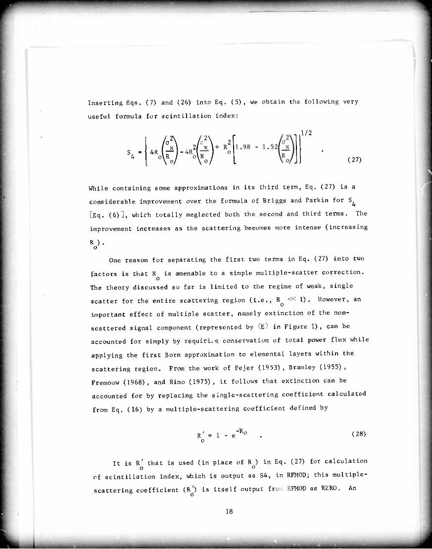
Inserting Eqs. (7) and (26) into Eq. (5), we obtain the following very

useful formula for scintillation index:

S4- "■Afhtffv R°

1/2

(27)

While containing some approximations in its third terra, Eq. (27) is a

considerable improvement over the formula of Briggs and Parkin for S

[Eq. (6)3, which totally neglected both the second and third terms. The

improvement increases as the scattering becomes more intense (increasing

R )• o

One reason for separating the first two terms in Eq. (27) into two

factors is that R is amenable to a simple multiple-scatter correction, o

The theory discussed so far is limited to the regime of weak, single

scatter for the entire scattering region (i.e., R « I)• However, an

important effect of multiple scatter, namely extinction of the non-

scattered signal component (represented by (E) in Figure 1), can be

accounted for simply by requirü g conservation of total power flux while

applying the first Born approximation to elemental layers within the

scattering region. From the work of Fejer (1953), Bramley (1955),

Fremouw (1968), and Rino (1975), it follows that extinction can be

accounted for by replacing the single-scattering coefficient calculated

from Eq. (16) by a multiple-scattering coefficient defined by

R = 1 - e c

(28)

It is R' that is used (in place of R ) in Eq. (27) for calculation o 0

of scintillation index, which is output as S4, in RFMOD; this multiple-

scattering coefficient (R') is itself output fro RFMOD as RZRO. An

18

,... . . . . . ^-.-. .....*■. >.., —-|,|,t , n ,

«WiW> ji ■"•"■'■"■", '

important task for the second contract year is to find an analogous

multiple-scatter correction for a /R and the related quantities UJ/R r x o o o

and 6. Presently, the latter two parameters are calculated from Eqs.

(26) and (24), respectively, on the basis of Eq. (23). They are output

from RFMOD as BMAGR and DELTA, respectively, for use as inputs to the

second channel-model code, DIST. A single-scatter approximation warni-g

is printed if R Ä !• o

Once R', |B j/R , and 6 are calculated, then application of the o o o

Gaussian-statistics hypothesis permits calculation of any desired first-

order, signal-statistical parameter. The calculation of the intensity-

scintillation index.

A ((A2 - (A2))2)1/2

<A2> (29)

as described above, is an example. An analogous phase-scintillation

index may be defined as

rms i <(l - <$))2>1/2 (30)

= «$2) - <$)

2)1/?- (31)

Given the phase reference chosen in Figure 1, it is well known (e.g.,

Beckman and Spizzichino, 1963) that under the postulate of Gaussian

statistics, the joint probability density function (pdf) for the real,

E , and imaginary, E , pa x y

E, is given by

rts of the received signal's complex amplitude.

P (E ,E ) = xy x y

2TTO O x y

2 2x/r : Vl - p

exp 1

2D

VE - T1)E E -2 ^H

a a x y

2(1 - P )

2

(32)

19

-■^i— ■■ * . ...„..^^—_,. -.-^ ^ggmm^|M^^^^^^^ _ M ^^„jto^^^^^^^^ _ J

r —-—-— *m^*i

where p = a /o a and where 1) may be calculated from Tl = vl - R and xy x y u

the a's fromEqs. (7), (8), and (9). The individual pdf? for amplitude

and for phase can be calculated by changing variables in tq. (32) from

component to polar form and then integrating over the other variable.

That is.

and

2r

P(A) = 1 A P (A cos I, A sin i) dl xy

p($) =1 A P (A cos I, A sin i) dA Jo xy

(33)

(34)

Analytic solutions to the integrals in Eqs. (33) and (34) have been

known for some time in special cases (e.g., for Rice statistics, in which

a =0 and a = a ) , but not so for the generalized Gaus.-ian statistics xy x y needed to describe scintillation. Recently, however, Hatfield (1975)

has found the following general analytic solution for Eq. (34):

TT 2

a exp x

p(l) = ■:(i - o )

2TTO a A - P2 f*(l) x y 1

(1 - p ) exp fy)

2(1 - D )

. V2n(l - P ) + f2(*) ^ *■ e^c

f2(*)

/2(1 - P2) (35)

where / 3 2 '

f (») = Vcos I/O - 2P cos $ sin $/(>T a ) + sin I/O x y

2 x, 2

y (36)

2 and f ($) = "H Leos I/o - D sin 4/(0 0 ) J/£ (t)

2 x x x y i (37)

2n

. UHttHUWiUdAb^. MttHm^biu

mfF^mmmmmm mmmmwmmmmmmrmmm* <•"•' '' -m iKiiPimin

U>fortunarely, there is no known analytic solution for the moments of

the distribution in Eq. (35). Therefore, the distribution itself has

been incorporated in RFNOD, together with a numerical integration routine

for calculating its first and second momeu.s, as follows:

and

2TT

<*) -I i o (|) di

2r

<$2) = f $2 p (») d$

(38)

(39)

The results of Eqs. (38) and (39) are then inserted into Eq. (31) for

calculation of the phase-scintillation index, which is output as PRMS.

As described above, the signal-statistical outputs of RFMOD are

B' IB l/R 6 S , and $ . The last two outputs constitute an intensity o o o' ' 4' rms scintillation index and a phase-scintillation index, respectively, and

represent our judgment as to the first-order statistical parameters most

likely to be soupht by a user for synoptic purpoeefi. The other three

outputs are provided for use in posing more detailed questions about

first-order signal statisticr in particular cases, by means of the

DIST code

The DIST code is essentially a device for calculating and outputing

the amplitude and phase pdfs from inputs of R^, IBJ/RJ, and 6. For

phase, it is simply a matter of evaluating Eq. (35) for the given input

parameters and outputing the result as P(PHI) . Unfortunately, there is

no known analytical solution to Eq. (33) analogous to Hatfield's phase

distribution. Thus, it is necessary to perform the phase integration

over the joint distribution (32) numerically. This integration is per-

formed in DIST, and the result is output as P(A) versus A (the latter in

21

. ■ „■-■^^-*^—.,.■-,,,—^..,. . . -

""MnmmiHipppMP«* 1 ■ ■ ■ "^^mmmmmmm

units of undisturbed amplitude). In addition, the following integration

also is performed numerically:

P(A < V) ■f P(A) dA (40)

This resulting cumulative probability function (cpf) of amplitude is

then output as CPF versus 20 log V (labeled dB). Since the independent

variable is output in decibels, CPF may be thought of as the cumulative 2

distribution of intensity (I = A ) as well as of amplitude (A); it

represents the link margin needed to mitigate scintillation fading to a

desired reliability threshold.

22

1^. -^^— — ■ ■ —

'■ " •'>"■-•" '" IN« "I "-i ■•ll-lll.l ■"■■■■ll-- mpirs«p»iwiiwi*>p»ip"«w«wiw

III SCINTILLATION MORPHOLOGY MODELED

The major work performed on this contract was development and

implementation of the generalized scattering theory described in Section

II. The other important aspect of modeling the transionospheric scintil-

lation channel is description of the ionosphere's scattering structure as

a function of several variables. The structural characteristics that

must be described pertain to the strength, size, and shape of the radio-

wave-scattering irregularities and the thickness of the scattering layer.

All the relevant parameters appear in Eq. (16). The shape of the irregu-

larities is described by the ionospheric spatial spectrum LEqs. (11) and

(UyJ, which is characterized mainly by the power-law spectral index, v.

and by the ratio, a, of scale-size parameter along the geomagnetic field

to that across it. The size of the irregularities is scaled by the

cross-field scale-size parameter, a. The strength of the irregularities

is described by the spatial variance of electron density ((AN) ), and

the thickness of the scattering region is L.

In-situ measurements of the ionospheric spatial spectrum (Dyson et

al., 1974) show a remarkably consistent spectral index, corresponding

very nearly to the Kolmorov value of 4/3 for V, under most ionospheric

conditions; we have adopted this value as a constant in the model. The

irregularity axial ratio, a, also has been taken as constant, with a

value of 10, as a result of the data review performed by Fremouw and

Rino (1973). There is no direct measurement of the outer scale, a; it is

simply known to be large compared with a km or so (Rufenach, 1972; Dyson

et al., 1974; Sagalyn et al., 1974). We have found that a = 3 km pro-

duces a good fit to the amplitude-scintillation data analyzed by Rino,

Livingston, and Whitney (1975), and this value is currently employed as

a constant in the model.

23

mm**r*mmmim <•>" •' PWW-P^I—- ,"",,u

The remaining two ionospheric parameters, ((AN)2) and L, appear in

the scintillation calculations only as a product. We have set L = 100 km

as a representative value and have expressed the behavior of scintillation

in terms of the following empirical model for the rms electron-density

variation, ((AN)2)1'2:

((AN)2)1/2 = AN (X, T,D,R) + AN (X,T) + AN.(X,T,K ) e m n p

+ AN (X.T.K ) el/m' a p (41)

where '• = geomagnetic latitude in degrees

T = time of day in hours,

D = day of the year out of 365,

R = sunspot number,

K = planetary magnetic index. P

The terms in Eq. (41) are

AN = (1.2 X 10 )(1 + 0.05R) e

1 - 0.25 cos TT D 4- 10

91.25 exp

fT + 1.5

+ exp T - 22.5

F

exp _ M2

\l2/ -

3 if T s 22.5 6 if T > 22.5 (42)

AN 8 N / TTT \

= (4.4 X 10 )(1 + 0.33 cos —) exn fX - 32.5^ i 15 ,

AN, = (2.0 X 10 ) h

1 + erf X - 68.5 + 1.82 Kp -f (5 + 0.55 Kp) cos (TTT/12)

18.7 - 0.36 KD - (1 + 0.11 Kp) cos (TTT/12)

24

(43)

(44)

1 ._! ■ M ...... -.L.. .-- ■ .

...l*.,^!....^. -■. ..-.

- --- -- ' - -■ ■ - -^ "iimi i in ■" ■— —-"-^ — - — — ^„J—^

.•—p—i —— HHRP111 •w«i n»1' ■PVHPMPMII I H

and AN = (1.1 a

x 108) K exp P

f - 77 + 1.82 Kp + 4 cos (TTT/12)^

0.32 K«

(45)

Eqs. (42) and (43) describe, respectively, the equatorial and mid-

latitude behavior of scintillation, and the high-latitude behavior is

described by Eqs. (44) and (45). All four terms of Eq. (41) contain the

well-established nighttime maximum of scintillation. The equatorial term

also includes a seasonal variation, displaying equinoctial maxima. The

most complicated behavior occurs at high latitudes, above the "scintil-

lation boundary" (Aarons et al., 1969). Equation (44) essentially

describes the behavior of the boundary location as a function of time of

day and geomagnetic activity, and Eq. (45) accounts for sein*illation

that is directly related to auroral activity.

In the Fremouw-and-Rino 1973 model, the relationship of scintilla-

tion to geomagnetic activity was not included. The only solar-terrestrial

observable employed in the earlier model was the sunspot number, which

was intended as a measure of epoch during a solar cycle. However, it is

clear that the scintillation boundary migrates equatorward, along with

the auroral oval, with increasing planetary magnetic activity (Aarons

et ll., 1963; Evans, 1974). This was known at the time the 1973 model

was developed, but the dependence was excluded to avoid double accounting

for other aspects of scintillation behavior, such as seasonal and solar-

cycle variation.

Pope (1974) modified our high-latitude term to include a K de-

pendence without checking on the possibility of seasonal double accounting.

We have had five years of K values plotted and have found no troublesome P

seasonal dependence. We have, therefore, adopted Pope's basic revision

of replacing the sunspot-number dependence in our old high-latitude term

with a K dependence. We have not used his exact formulation, however, P

which deleted our earlier description of the variation in statistical

25

■^L ■-"■* ■ «MMMfiiktfdia IIIIüI—iMMii. nimünagiM,., .„^utamaannHB,,.

——' P?pi""P»IIW"I^IWP»"IHii»W?»W»«B»'W"^'W«

width of the scintillation boundary with its location. We find that there

is such a variable-width behavior in the in-situ data of Sagalyn et al.

(1974) ; it is described by the denominator of the error-function argument

in Eq. (44).

Having incorporated a K dependence in Eq. (44), it was a simple

extension to include the K -dependent migration of the auroral oval in P

Eq. (45). A more accurate index to use might be the auroral-electrojet

index, AE, but we have elected to use only K for simplicity. The two

magnetic indices, K and AE, are rather highly correlated, as shown in

Figure 4. To avoid the necessity for a user to specify two magnetic

indices rather than just one, we have elected to exclude AE from the

model unless later analysis of scintillation data shows that including

it would improve the model's accuracy significantly. In a similar vein,

we i.ave avoided including a geomagnetic dependence in the equatorial

term, retaining instead the original sunspot-number dependence. Further

experimental work is necessary before a reliable geomagnetic dependence

can be incorporated in the equatorial term; a likely candidate for a

magnetic index is D , the seasonal and solar-cycle behaviors of which st

are similar to those of scintillation.

In addition to the above modifications to the 1973 model, some of the

constants employed have been changed. These changes stem partly from

improved calibration of some data sets used in development of the original

model. The data sets in question (Aarons et al., 1963; Koster, 1968;

Joint Satellite Studies Group, 1968) were presented in terms of a hand-

scaled scintillation index, SI (Whitney and Malik, 1968), which only

recently (Whitney, 1974) has been calibrated reasonably accurately to S^.

It is still to be noted that the relation between SI and S^ must be

scintillation-rate dependent, and data characterized directly by S^

are strongly preferred for modeling.

26

■- " - ' -—■■ - - ■ -"■- ■■-- .--.■ ^■.—... lataWMiä

r mmmmmmmmmmmmmmm IIWJI««"

"

t

— o E o) o •-

5} < c

ffi

ii

_ 8

x

z

I —1 o re

-J

8 i z

8 i

8 S

8

—^ 8 CM

• . •

L^ L iliU Ol+o>| + »l+^|+^o|■,■'"l+*, IN I ♦ •■ I + O

cr a oc ^ O - O X

LLI

oi Hi Lil U ■E P a u S z D u

if ll

ai l! < - to <

D a

27

■ ■ -^ nmiM _^

WM«l IWW^^^W^^^t wmmi'uim m j IIIWIII|«II - IIWWW«W«W^WP^™

Figures 5 through 8 show the degree of fit between the model

now in RFMOD and several data sets that were presented by the observers

either in terms of S, or in terms of an empirical index such as SI, 4

which we then converted to P,. Figures 9 and 10 compare the amplitude 4

pdf and cdf calculated by means of DIST with corresponding histograms

developed from AT? 5 data provided by Aarons (private communication,

1974). The corresponding pdf for phase is shown in Figure 11; no phase

data exist at this time for comparisoi .

IV THE CHANNEL-MODEL CODES

Of the two computer programs, RFMOD and DIST, the former is by

far the more complicated. It is a modification of the program BPMOD,

described by de la Beaujardiere and McNiel (1971), and consists of the

routines listed in Table 1. Its very simplified flow chart is shown in

Figure 12. Using RFMOD consists essentially of preparing input cards,

of which there are three types: (1) a title card, (2) namelist cards,

and (3) a changing-parameter(s) card. Three sample sets of input cards

are shown in Figure 13, and each type of card is described below.

The title card is used to assign any desired title of up to 80

characters to a calculation case or series of cases. It is read by

the driver program, RFMOD, into the array LBL with a 20A4 format, and

printed in the output by the subroutine IMPRIME; it ha^ no effect what-

soever on the rest of the program. Any number of cases can be run

under a common title, which will be printed in the output for each case

The namelist cards are used to input the fixed parameters for a

calculation case. They are read by subroutine READIN, by means of fie

namelist INPAR. The user gives the name and desired value for each

quantity listed above the dashed line in Table 2 that is to be fixed.

The number under the heading K in Table 2 is an index used in the

28

■^^"■■^^^■~"" ' " ' PWll i. •»■.in- IIIII»III -»vn^qpB^^B

-i—'—r -I—'—I—r-

J__. I i_Jl , L

I S » Xj 8 <? s 8 d d o d o o o

»6--X30M NOUniiNOC

1 — ^ UJ I z z 9 t- O O 2 2

§ <<§;

LCU

V

AR

L

AT

I (1

96

1 < -J d DC U < L_ UJ

F M

OD

EL

E S

EA

SO

N

SIT

Y-S

CIN

B

Y

KO

ST

EG

ION

8I 1 O i z -^ ^

ISO

N

TH

T

INT

E

ED

(X

RIA

L

1 < ^ 5 m ^- ü. - 5 £ < llilg 1 O o •- O UJ

■ UJ

o cc ( 3 ü

I 5 LU <

z o

0 < u _i LU Q O 5

to

DC

e LL CO < o o 5 ?• x UJ O w - Q UJ i- i I < - 1- EC Z ■7 < o

< H 1

z d ^ EC t- D Z LL

UJ Q U h

to CO

ti 0 ^

5 B V z _ z CO 0

OJ UJ

IS X UJ DC o —

5 5 S M--X30NI NOanuNIOS

o =; £

in

OJ DC D (9

29

I ■ - --■ ■ — ■ -■■ ^-l^^^^y^l

r rt^m^mm^mm^^^^mmt^m^mm i ■ ■ I I ^^^w» F-JÄIHW-i"^1»1 JWIIPWiJi« I II il* I wwum****!!*

f M ft

/ I i . - ■■ I

8

(so

lid

ON

OF

E

X,

3IS

- N

S

LA

TIO

N

yS ♦ ii

I ' -\ i 1 ' I

r -> a

LA

TIO

NS

V

AR

IAT

I IO

N

'ND

I G

NE

TIC

B

Y

EV

A

SC

INT

IL

^-^-7—-- )^\ _ in

a 4 ^*N. vX -

♦ ^^^ ̂ ^NJ ffl a , 1- < -sr _i

- ♦

^S. 0

♦

^v a

5&: S«

^ _ C

AL

C

UD

INA

N

TIL

LA

G

EO

M

(sym

bo

l U

RO

RA

♦ .tw 4 y |

Bpa^fii

■

« ■

OF

MO

T

HE

LA

E

NS

ITY

-

ST

AT

ES

O

BS

ER

VI

TH

E

SU

- + V s|

AR

ISO

N

) W

ITH

IH

z I

NT

T

HR

EE

A

NC

E,

1 N

EA

R

DA

RY

■ V/ i. O. " 2 CD m Z

- V/ V/ A\ a o a

I 1 ([- 5 Ü I OC EC £ D

o 5 § O D ® o 0 o ^r u- t- — on

■ ^ CM ^ «O'

CO

1 1 . 1 1 1 IP o LU

IV S 8 8 s 1 o* o 6 o o o o o

»«••X30NI NoumiNios u.

5 5 5 3 »«--xaoMi NoumiNos

30

Z) o -J > z < < - O OC z

UJ ^ |_

9 _i < 5 Z d a r ^- o2? ^ Q O

O T J - t H <5i ft -^ ^ ^ a- LU

O o —

Q Z < LU oc - z Q2 z a < LU

OC

3fi 2 ? Q t < <

>% LU S

K z > -

2

L

mmmmmmr !■■ ' «""I11 '"•""W1 ■

3.9 -

S J.o -

h

Z UJ 5 > t-

< CO

O OC a

O.S 1.0 I.S 2.0 2.6 3.0 3.5 *MPUTUOCA)NDQTU«SED «MPUTUOE

«.0 4.9 S.O

FIGURE 9 COMPARISON OF CALCULATED (smooth curve) PROBABILITY DENSITY FUNCTION FOR AMPLITUDE WITH OBSERVATIONS (histogram) OF ATS-5 TRANSMISSION AT 137 MHz, MADE BY AARONS (private communication, 1974) THROUGH THE MID-LATITUDE IONOSPHERE FROM NEAR BOSTON

^ > >

*

-.-i"»

i

0.001 ■30 26 •20 -16 -10 -5 0

SIGNAL STMEN0TH--0B

FIGURE 10 COMPARISON OF CALCULATED (smooth curve) CUMULATIVE PROBABILITY FUNCTION (cpf) FOR INTENSITY (or for amplitude) WITH OBSERVATIONS (histogram) FOR CASE IN FIGURE 9. (Calculations of cpf are intended for use in assessing fade-margin requirements.)

31

— - -- ■■■----- ...^--.-J- ^ —.. -^ ■^-.. — —

r — ■■■ ■'

——— wmm. — -^-^ -^»

z LU □

< CQ

o Q.

0.020

0.0«

0.0)6

O.OK

0.012

0.010

0.008 -

o.ooe

0.004

0.002

-I—■"

-200

-i—'—i—•—r

S- - 0.282 4

-180 -100 -SO 0 BO PHASE «NOU-DCOnCO

_. 100 IBO 200

FIGURE 11 CALCULATED PROBABILITY DENSITY FUNCTION FOR PHASE FOR THE CASE IN FIGURES 9 AND 10. (No observed phase üata exist for comparison.)

32

■t. -—- - ■"■—"- ■ -— I llll J

■ ■ ' 1 ■■ I 1 «"I"! IWP-^—

Table L

ROUTINES IN PROGRAM RFMOD

Name

BLOCK DATA

SUBROUTINE READIN,

with ENTRY INC

SUBROUTINE SCINT

SUBROUTINE SIGS

FUNCTION RMSDN

FUNCTION RFBPT

SUBROUTINE FINDZ

SUBROUTINE MGFLD

SUBROUTINE AZNSIDE

SUBROUTINE COORD

FUNCTION ERF

SUBROUTINE CPRMS

FUNCTION PHAS,

with ENTRY PRT

FUNCTION FL, with

ENTRY F2

SUBROUTINE SIMPA

SUBROUTINE IMPRIME

Function

Initializes common parameters.

Performs program inputting, and increments the

changing parameter(s).

Controls the basic scintillation calculation and

provides quantities needed for SUBROUTINE SIGS.

Performs the bjisic scintillation calculations.

Contains the worldwide model for strength of

F-layer irregularities used in the scintillation

calculation.

Evaluations the diffraction integral by an

algebraic approximation.

Computes the reduced distance from scattering

layer to receiver for use in evaluating Fresnel-

zone radius.

Contains an earth-centered, axially tapped,

dipole model of the geomagnetic field and cal-

culates the geomagnetic coordinates of, and the

field components at, a specified point.

Given the latitude and longitude of two points,

A and B, computes the azimuth of B as seen from

A and the great-circle arc AB.

Calcul?tes coordinates of a desired point on a

specified great-circle arc.

Computes the Error Function.

Controls calculation of rms phase.

Evaluates the Hatfield phase distribution of

a scintillating signal.

Provides ir.tegrand functions for evaluating

moments of phase distribution.

Adaptively performs numerical integration

using Simpson's rule.

Performs program outputting.

3 3

—- mi >. HWUIII.II mtivm'mim«»««*«' tmw^^mmmimmmm*****m

READ THE FIXED PARAMETERS.

READ THE NAME OF THE CHANGING PARAMETER AND ITS START, END. AND INCREMENT VALUES.

CHANGING PARAMETER = INITIAL VALUE - INCREMEN

I INCREMENT THE CHANGING PARAMETER.

I n COMMUTE INTENSITY AND PHASE

SCINTILLATION INDICES AND PROBABILITY-ELLIPSE PARAMETERS

I STORE ALL PERTINENT VALUES.

DISPLAY THE VARIOUS PARAMETERS FOR THIS CASE, AND THE VALUES OF THE SCINTILLATION INDICES

AND THE PROBABILITY-ELLIPSE PARAMETERS

J LA-1079-28R

FIGURE 12 SIMPLIFIED FLOW CHART OF PROGRAM P.FMOD

34

..- — .-. ....~.

mmmmmimmmmi^mmmmmmmmmmimmmmmm^^mm

CO LLI

LU

■^s

Q tr < o

D % < ? o Q-

-s

H 9

Ul UJ 7 Q _J 5 < tr t < I < H Z O <J

3,

-N

s ^ CNJ S M * a kTt

c _ r-j r «-» ^ ■ i^

«? — rsj ■ t-i •* ■ u-s

IS *- <-j c r-i •W K irt

■ — f^j ■ r-l -» H U")

to c

Q O 5

IP ._ r>. i r-l ^■ IC kO UJ C f— OU : <n ft QC 1 ,— t^, - <■-> m R *r» U3 S »** «o X «n S

p _ r-j ■ ro v P ■J-> m P -» BO P wi P

< i _ C-s^ C ro T P Ul LD P r- «o B CTl 2

^ ^. r-i fC m ** c in to F: r— oo ■ CT» t-

■ _ OJ E r-l ^r E LO UD S r— so e m S DC I ^ Cs. S r-> ■«■ i; UT to :;, r— oo S

o I ^ CN ^ r^ »T r^ m <o S i— CD S CT> 3 _ rsi c-i ■**■ s m U3 S r* •o £ en £

rs ^ rvj 8 n ^■ I u-> UJ " *^- oo £ oi S CC s ^ r>i 1 (-> t 1 in to £ r~ oo | enffl a. s *- f^i 1 d •W a m LO S »- oo Z CT^ S

rs ^. fs. 1 r-i « 8 m LO s •— oo en 3

§ a — c-d Tn n V ;.■ u-) «a 3 i— oo '^ en 3 _ CN. - r-i * r,. m «■ 5 r^ •e Z CT» 3

I _ «^ | «n ^r ^ m to 2 r- •a s o»S u. s — rsi ■1 r-, -» ? u-» to S —- so ?; en S

a *- Csj | ro « S m to S r— •• a a>S tn w— C-^J B r-> -t s> UO U3 « r— co a en S a ■ — r^, !f n-» -* ■ LO l..- Ä »- CO | <n Ä

< n — CN| « f-. •*T ^ m M K r- ■o Yl o> K

R ^ rvj R r^ •f 1 m to X -^ oo r. en S

^ rs. ■ c-> ■f a LO to S P* •o 7 en .,,

91 ~- rx a r-l ■^r a m to S r— oo r-; <n ■ r- r>* n r-> ■«■ s to to Ä •** «o ■ en s 1-

S — ox I <-) •■t- ^ UT to 5 r- ■o r er» SQ 5 f^g 9 I CM * I e^j f '

V — es» S

e*M 5 r*»

^- ot E n

*- csi R «*» — «-* « « -- CN fi f»

^- M I n

— CsJ R «*» »— rsi R c»

— fsi S ro

•— CSI S €*»

•— «si ^ r»»

R to K m

K in R tr»

■ «n

to 3 i u> 7 i u> V i (O w I

to 5 I to ^ I

to S to ^ «« « to S to s

- en ^ u.) • ••i 3 en 3(D!

1 * a» , i

! S "lZ

■ R w» S3, r— oo S en !

i— •• K en «L

to r. r- » ! CD ^ n- OO ;

J S ' to ?■ I

s; <n a

S «n fi

oo ? CTi 3

a. Z

Q.

<

n

LU

o

"i "''

t a ■» . cx >

" m tO to c _ no ,. "-I

m ■a - — *M - M -*■ f m to ♦» r— ro <- Wl -

—' C3 ■■ — t^ ■ CO *r * u-) ■■ UJ ^ 33 "• ^ J-

) o ^ — CN* IO r-j •*■ m i to M r— «5 •n ^1 -1

i« ^ e^i » m « u-J to • ^» OO • en «

m — _ J« ■** ,-, JT U"' r» r— CO r^ tn N

J ^ r- ^ esj « ro ■~r »» u-> _J ** t^» no 0) r«

-J

' -J" n ^ m to CD

35

■■ ■ ■ ■ ■ MMM^MHMBMiMMMHMaMMIMMiM^.^

PMMRIIWI Uli I N« mmmmmmmmmmmi^ i****

Table 2

DATA-CARD VARIABLES

K Variable Name

1 FREO

2 SSN

J DAY

4 TIME

s RLAT

6 RLON

7 HK

8 TLAT

9 TLON

LO HT

11 FKP

II

Unit

Megahertz

None (floating point)

None (floating point)

Decimal hours

Decimal degrees

Decimal degrees

Meters

Decimal degrees

Decimal degrees

Meters

Decimal value 0.0 through 9.0

None (value 1 or 0)

Definition

Frequency

Sunspot number

Day of year

Meridian time at iono-

spheric penetration point

Receiver latitude

Receiver longitude

Receiver altitude

Transmitter latitude

Transmitter longitude

Transmitter altitude

Planetary magnetic

index, Kp

Data flag (see text)

12

13

RCRD

TCRD

Decimal degrees

Decimal degrees

Receiver coordinates

TranFmitucr coordinates

common VARPAR to identify the parameters. The user may list the fixed

parameters in any order on the namelist cards.

A parameter input on a namelist card will keep the specified value

until changed by means of a new namelist card or until input on a changing-

parameter(s) card. The first colmtt) of each namelist card must be blank,

and the first characters on the first namelist card must be &1NPAR. The

last namelist card in a sequence must terminate with the characters &END.

}6

fl^^M^MtetfiiiMili , „ _. „-^.-.-.

mmfi» mmmmmmmm^mmmm mi, i «liiiiiiiinnii

•

The changing-parameter(s) card is employed by the user to select the

independent variable(s) for a given calculation case. He may choose

either of two program modes. In Mode 1, he chooses any one of the param-

eters listed in Table 2 for which K is between 1 and 11, inclusive, and

inputs its name on the changing-parameter card. In this mode, the first-

order signal-statistical parameters, including S^ and ^rmg. are calculated

as functions of the single changing parameter. In Figure 13, the cards

identified as Set 1 are for two sequential cases run in Mode 1, under a

common title.

Mode 2 permits the user to increment the position of either the re-

ceiver or the transmitter along an arc of a great circle. In this mode,

both the latitude and longitude of the receiver or of the nransmitter be-

come changing parameters, and the signal-statistical paramete-s are cal-

culated for equidistant points along the arc. Mode 2 is selected by naming

RCRD or TCRD on the changing-parameters card (see Table 2). In Figure 13,

the cards identified as Set 2 are for a run in this mode.

The required contents of the changing-parameter(s) card are listed

in Table 3. Note that in Mode 1, if the final value of a changing param-

eter is smaller than the initial value, the increnent value must be speci-

fied as negative. Absence of the required negative sign in this situation

will cause the run to terminate, and an error message will be printed.

After reading a set of cards, the program will keep the same title

and read only namelist and c nging-parameter(s) cards, so long as II = 1.

After encountering II = 0, it will read a new title card. The program

will terminate if the name on the changing-parameter(s) card does not

correspond to one of those numbered 1 through 13 in Table 2. Thus, to

terminate a run, the user may prepare a changing-parameter card contain-

ing an unfamiliar word, such as the FINI appearing in Figure 13.

37

- ~ - ■—■^—>.^.

r PW^iHli^W» ■MDPMIP« ■■umpipm^iiP^B^^wwwii^^iw^

Table 3

CONTENTS OF CHANGiNG-PARAMETER(S) CARD

Columns

I through 4

9 through 16

17 through 24

25 through 32

33 through 40

41 through 42

Mode-1 Content

Name

Initial value

Final value

Increment value

Mode-2 Content

Name

Initial latitude

Initial longitude

Final latitude

Final longitude

Number of increments

Symbol

in Program

Name

Al

\2

A3

A4

NA5

For model development and testing, we employed a plotting routine

in conjunction with RFMOD to produce graphs such as those in Figures 5

through 8. The available version of RFMOD provides an array that the user

may employ with his own computer peripherals. In the absence of user

modification, the array will be output in tabular form along with identify-

ing information, as shown for a test case in Figure 14. In the case shown,

the changing parameter was the latitude of the transmitter, which was

taken to be in a nolar-orbiting satellite passing over a receiving station

near Boston (namely, the Sagamore Hill site of the AFCRL group headed by

Aarons). The changing parameter is followed in each row by the azimuth

and elevation of the satellite, the three probability-ellipse parameters,

and then by the calculated scintillation indices. The input cards for

this run are identified as Set 3 in Figure 13.

It is envisioned that a user will inspect the values of S4 and/or

PRMS predicted for his communication link by RFMOD and then decide if he

wants more detailed" signal-statistical information for a particular

situation. In the example of Figure 14, for instance, he might decide

Hby i

38

— " ll«l II ■lllllll UIIJIII p l in . HI 11 "•-—-"B^P^W

ii A m r rnpV IS-r'

M z — X o a

1 < Z I wU O 1 (Si •-• 1 U 1- • a < 1 -1 1 o -1 1 a •-• 1 o t- I Ik Z i z ~ i < (J 1 t- IS. 1 1^

i b. 1 >- X I LC

1 I Q u. • Ul X 1 a > t 5

1 _p C, 1 IM lb I > U 1 lu 3 1 a C 1 C 1 _. • a i ul « a i O •-

i c z 0 1 J o

U.< I o V • «J u. « 1 I-«

_- • a _• 1 1 c «

A. 1 X J 1 u. *

c & UJ I >- 4 < a. ~j

Z)0 O-l -JZ

1 m •— *-

X X X it

o o • c o ^- o o

CM O II • •

o X -♦ U o- o z »-' a II II *

-J -1 •J <

iT c Cl

19 (9 u. lu Ui O a o 1- a. oc —' I— ^^

c m •

• oc a. .— ro rv< m

II II m IS u. > i z aJ < o o 3 o _l -1 in * z 5 •

r^ IS i- « UJ « c _J D II m U • • -1 o • < 2 fM O

¥- ■•

IS) O a. ■

I (SI 1- K z <

3 —t

a IS o u. IS) »s,

UJ UJ o N. ►- *- u. 1 <. « IS S z z • 2 »— •—

_' c c c «: IS • c a a z • o c • o ♦ o o

►- •-» If. o u U- ►-

► -■ a a » 3 I a ui IS Z > > ►- z ■3 <-l •-« >- o <_ z UJ ►- X ul (J z 4 »- 3 UJ IS) «t J a X z * a Ui ■ • z a X • •-• u. 1-

(M«A«'i>(\j-<sis>'Om ISI r-^moorfio^r'iW'" X •••••••••••

is. »»• ♦miro>mi>'"i^*^

a

z

is

X u,

a

z

X

z a

I

u. a

a

2 a.

o x x

(M o-^tvjrurnoruo or*- X ♦ I» ÄwiK •!♦"•• • ^,^.«air>c(\ir-«c«

• •♦•••••••• * ♦(^r(\i(\joj(Vcvjr>-*«

» ccMn^iTirwcxjca

(D'-.'-^o-*iS>-*lf*'— IT*— »^►»«»lOIVj^'* '^'<VI

«xisim^c-'C'^iroC'-

4 ^cnir. cismc ^-•« >MC\J<y»ifl(»'il>'T>IM'<

c- oooooooooo c cooocooocc.

c c c c c a a x a a

t- c e. o c

«1 WWWI'll'IMWWrtM

-. \j vi -n i ♦ * n ui -o i)

c z z a

M. LU O X

I

•- IT

u z

^ *

19

- - - - - --

I""-1" "iiipw II. I r^^wmmm ,mm*«*mwm*mm,mmmmv« • ■"■ "'" '""■—w««!IPI»pimii!i" ^t

that he wants the full first-order distributions of intensity and phase

for the case in which S4 on his channel is .538 and PRMS is 32.835 degrees

To obtain the distributions he would employ DIST, inputting RZRO = .371,

BMAGR = .924, and DELTA = 3.419 degrees, on a single card in F10.3 format.

The DIST code consists of the routines listed in Table 4.

Table 4

Name

SUBROUTINE PDFI

SUBROUTINE PARRAY

SUBROUTINE GAUP

FUNCTION PR

FUNCTION XINTGR

SUBROUTINE PDFP

SUBROUTINE PHAS

FUNCTION ERF

SUBROUTINE CPFI

ROUTINES IN PROGRAM DIST

Funct ion

Controls calculation and output of probability density function for amplitude, by means of one- dimensional integration over two-dimensional Gaussian probability density function.

Initializes amplitude array for SUBROUTINE PDFI.

Controls calculation of Gaussian probability density function.

Computes two-dimensional Gauspian probability density function.

Performs integration by Simpson's rule.

Controls computation and output of probability density function for phase, calling SUBROUTINE

PHA3.

Evaluates Hatfield phase distribution.

Computes the Error Function.

Calculates and outputs the cumulative probability density function for amplitude or intensity (expressed in dB) by performing Simpson's rule integration over probability density function for amplitude.

40

^MiMIHMMllitil ,,„ I-, I

W""1" -11-«I— pinpHMippi. iliu uiiMmmn^^mim'. mmmmmmmxM.v •—" '^i

Again, for modeling we employ a plotting routine in conjunction with

DIST to produce graphs such as those in 9, 10, and 11. The available

version of DIST simply outputs the array from which such graphs are made,

in the line-printer formats shown in Figures 15, 16, and 17. As with

RFMOD, a user may wish to employ DIST in conjunction with his own plotting

routine or in some other output form. Alternatively, he may wish to

reformat the array listing, perhaps outputting fewer values and possibly

presenting CPF in terms of percent or decimal link reliability (the one's

complement of CPF) rather than directly as in Figure 16.

V CONCLUSION

It has been our attempt to develop a channel model that may be used

conveniently for calculating first-order signal statistics, expressed in

a format relevant to systems application. The resulting codes, RFMOD

and DIST, represent the first-year output of a broader effort to

definitively model the transionospheric communication channel. These

codes are to be augmented by routines to permit calculation of second-

order statistics, such as fluctuation spectra of amplitude and phase, as

well as signal correlation at spaced receivers and across bands of

frequency. Moreover, the existing version of RFMOD is likely to evolve

over the next year in two important ways.

First, it is intended to modify SUBROUTINE SIGS in RFMOD to fully

account for multiple scatter. Theoretical work now underway is hinting

at a possible form for the modification. The single-scatter theory

described in Section II of this report describes the simultaneous rota-

tion (increasing 6) and circularization (decreasing |B0|/R0) of the

first-order probability ellipse for the received signal's complex ampli-

tude (illustrated in Figure 1), as the wave propagates away from the

scattered medium. In the single-scatter limit, the ellipse emerges from

41

^^^^^^^^^—^^^^^^^^-—^^^^^^^ .- - .... ..■^„. I ngj

r^ —■'■"—"■ ..ni.........11...... , MP"WW|MM

1

•-•••«««^•««•-•««jgs^ssssssssss:::::::::::::s:::: wOC(VC\-cr-'-fVfctj' ♦a*—r'^ru— cccce

_ XJ - —

*,************£££££*££££££££*££££££££££££££££££££££

^» 3 o o o oooooooooooo o o c. »oo

OCSCJOOOOSCC- COOOOwCCOOC

sea1 o—«iin^ *■* 3 o

■#mf*ir»>^*mr^c\i»r>(y f 9 rfl JB

^ f\i ^ -»

< tr U o cc

U. o

00 DC UJ > LU _J 00

< j =) c =- -^ c . o ^. a J o =• —

3 3 O O O 3 C

JOOOC ooooooooc- ooooo

^. M — ^

,£ J.!.! M,!~.I,I« IJM «CM'CM WMNN» tnmin«*»mn«t •••««««•« «

M>aau9««M«'q««»«>M«»*2*9^*«*s»SS2S2SSSSSS

— l\i (\i -^

• ••■«••••••*• ••• ^- f\* r\j ^

5 O u.

P o. F b o ■D a LU Q D

Q-

<

M _ P!^ «T«! pi M M pT w M M fJ M w M M M M m m n n *» n a m m n « « « « « « « # • «

• • • • • • ^ (M ru ^

.

>■ c

i/ a ft w

-• H J O •-■I CD (St 4 n B OX xo 1 u.

M MMf xcr Cf-ixim^tror^ao-

LU _l a.

< X

LO

S 3 a

■ r- ir n (\. •£ a r^ <0'i-fvarr.fvxnr-^cccccoecccc,cc;cceccocc ^

ilillllliirMliijIiHIMiUliilMsUtHHIMUIUM

42

Mi ̂■■difcl^iiiMriii 1 —" -■—

r"" - ," '■ " ■ ~-—- "" ^««p^"»»w«~^l

1

4 \.l -"•

,. ■ p« i^ MIA • ji •« JI i^ m # • • o c o o w c • e • o o

«ill ^^,«,^^.^-««-» — i

_j -«jli NiAi « '~-3-*J''*t\^*X. * <J s\ ?y I\ > * H f\i IS J-

jit *'\t i ^•\*'ri-»xt-o^--0'o>o»'-«— ■yrvrnri'n

Z

*.TJ". -vi — r\jr>#lnx>h-xxJ-J,o — -^—fti^^^^'

«ill mmmmm** •* mm

< •••••••••••■•••••••■•••••

x, cx'vj'^r\,r'X'v—x-#'^X'T>J^rT>^x*'MX^ X<»

R4 I I

-. j. _Joxxr\i'*>"fcnj'M-ttr>Ä<^->c:--,=>o-^t- — ^^J-*0

o a ooLsfMxr^ji^jiinx^^cicocooc-ooooo

x _!'-_!_!-^_!

^. -iii ^-^.-.^- — «^-*«

U) ■ • I

J c- ec—mm — XJ. xa-Ta'TCi-cccccc.wJwO-. • J: cocom^xJ-o^J'a^cooc.ucciCooc.o

u • "•*'•*********_!*_!_! —

U (NJ

>. o cc,5i>r--*-*a»0ümm(\iOh-<— xfxjf-'^^ — J^^r>r,fc

^.(i ••••••■••••••••••••*•**'* »-(» i)f\j^}m— ^r><irfr-KX*<TuO'-'-njf\1(\jmm

J Oj-lll ^^.^^.^^t-^r' — 4 II x x < X r u <rcAjf*#r-c_ffi/ic4ac_ccccccccc-cc C u. oocmxr-^XwJP'fXCTO'ococcocc.ctoc.c

> II h-a O »-x i3 ♦xmaur- —4>xr\ir,»min(^a»(M-'»fc-»iytn^fvjMt?'^

5

00

< (9 5 CE a.

o

>

CD < < > < 5 O CC

F o ■a 0

a.

<

•JJ

to

LU CC

a

ifc. I

mm i... mmmmw mmmm mm -^-w

r-.'-; ! • .■ ■ t1. " f CD?V

—. L- _ .j .- i o x ^' w - — —' X ctc-ccc-occccc.

^oj>*r> I (M « i^ O n 4

1 3 o a JC-OOCrO — CO 3 O O _3 O ■ J JOOO

£ 3»0 O^'NJiJl • f*l M ^

CO

< a o cc 0_

^ •••••••••••• -..iii ^ ^ ^ i i i

a. ^C-OOOOOOOOOC

^

1 (I £

a a a i^

_> „ _ i i i ^ « -. I i l

Z o cc LU

> LU _J CC <

< > <

Q. •••••••••••• 5

Ofncr^.#(\i r*) e o- f\j j) ~~ -—.111 »M CC III LL

a occ3occ3=.ooo& Q_

- 5 X cjc»xp--o#tf>*i/r-«5'0 ^ a •••••••••••■• __

TT7... — . « 3J3000-VJOÄ0030 ^ »-• oooof^cy^xmccoo 3 X ooooooooooooo X a. ooo^ooooooooo a.

a a. o

• i » < — c'j^O'--#nr-xc/Cc-= X •-I OCOOrM»TX*OC.O-S QJ 1 cccsec-oc—c-coo *" Q. 00005:00000000

fc ■ * ■ " ' J.

I rr»(\i'-*oc*^x<\*',ri-*in"0^ UJ a ••••••••••••• ,—

M^M • I I mmm ^ • i i g

— oooccrv-^ccioocc U- « c.coo^J'^xu.ococ g ja»oo33-*^-»3JO .i OC JOOOOOOOOOO

44

M ■Mt^dMüMMUMMMMMiMIliMriill MMMMiMMi^

1" »' ^mi^^mmm —-—"— ™—T-—————- W" ! ' '

the scattering layer highly elongated (|B0|/R0 W 1) and oriented nearly

vertically (6 « 0) on the complex plane.

Multiple-scatter calculations for the special case of normal inci-

dence on the scattering layer show that some circularization (|B0j/R0

M e"^), but no rotation (6 M 0), is produced Dy the reseat.erings. This

is an intuitively understandable result and, if corroborated by similar

calculations for off-normal incidence, is expected to lead to a multiple-

scatter correction for |ß0|/R0 analogous to Eq. (28) for R0. It will

presumably also lead tc a modification of Eq. (24) for relating the

ellipse orientation to its elongation at the receiver. The result is

certain to be a reduction in the third term of Eq. (5) for intensity-

scintillation index as the fraction of flux scattered (Ro) increases.

It will presumably limit values of S4 to something near unity and improve

agreement between calculated and observed values for moderate to strong

scintillation.

The other important area in which RFMOD is expected to evolve is

that of scintillation morphology, which will entail updating of FUNCTION

RMSDN. As more definitive scintillation data become available, the model

of electron-density irregularity strength contained in RMSDN presumably

will be improved by a process that may be viewed as calibration [i.e.,

the main changes should be adjustment of the coefficients in Eqs. (42)

through (45)]. This will be particularly so in regions where the model

is currently calibrated in terms of ad hoc indices such as SI instead of

in terms of S,. One such region is the important one centered on the 4

geomagnetic equator. Useful equatorial data are expected from observa-

tions of the NOAA ionospheric beacon on board NASA's ATS-6, particularly

measurements of S, at 140 and 360 MHz. During periods of weak to 4

moderate scintillation, estimates should also be obtained of 0^

at 140 MHz. The ATS-6 observations also will provide histograms

4.

-- - ^- -^r^.L^^L-.^.. . ... -..- . ........ ....■■

—- 11 "■,l1'

of amplitude (under all conditions)) and of phase (under conditions of

weak to moderate scintillation) for testing the predictions made by the

DIST code.

Pending the improvements described above, we offer RFMOD and DIST

as the best way to estimate the first-order signal statistics to be

expected at the output of a user's transionospheric communication link,

short of performing a series of observations over that particular link.

It must be remembered that the estimated values are those expected for

average ionospheric conditions in the observing situation (frequency,

transmitter and receiver location, time of day, K . etc.) specified by

the user. There is presumably some statistical distribution of each

parameter estimated about its calculated value, and the present model

does not account for such statistical variation. Possibly of equal

importance, the model has yet to be subjected to testing against observa-

tions above 400 MHz (e.g., in the SHF band).

4b

i M^MMiMM —- - —

r II»"1«"1' «w—mmmmm^mmm P | '|'«| <<i ^-~-™ "«" i »^»^^^ww T|

REFERENCES

Aarons, J., J. P. Mullen, and S, Basu, "Geomagnetic Control of Satellite

Scintillations," J. Geophys. Res., Vol. 68, No. 10, pp. 3159-3168

(1963).

Aarons, J., J. P. Mullen, and H. E. Whitney, "The Scintillation Boundary,"

J. Geophys. Res., Vol. 74, No. 3, pp. 884-889 (1969).

Beckman, P., and A, Spizzichino, The ScatterinR of Electromagnetic Waves

from Rough Surfaces, pp. 119-136 (Pergamon Press, New York, New York,

1963).

Bramley, E. N., "Some Aspects of the Rapid Directional Fluctuations of

Short Radio Waves Reflected at the Ionosphere," Proc. IEEE, Vol. 102,

pp. 533-540 (1955).

Briggs, B. H., and I. A. Parkin, "On the Variation of Radio Star and

Satellite Scintillations with Zenith Angle," J. Atmos. Terr. Phys. ,

Vol. 25, pp. 339-365 (1963).

Budden, K. G., "The Amplitude Fluctuations of the Radio Wave Scattered

from a Thick Ionospheric Layer with Weak Irregularities," J. Atmos.

Terr. Phys.. Vol. 27, pp. 155-172 (1965).

de la Beaujardiere, 0., and D. McNiel, "A Fortran Program for Calculating

F-Layer-Produced Scintillation," Final Report, SRI Project 10'9,

Contract NASr-21551, Stanford Research Institute, Menlo Park,

California (December 1971).

Dyson, P. L., J. P. McClure, and W. B. Hiinson, "In Situ Measurements of

the Spectral Characteristics of F Region Ionospheric Irregularities,"

J. Geophys. Res., Vol. 79, No. 10, pp. 1497-1502 (1 April 1974).

Evans, J. V., E-i., "Millstone Hill Radar Propagation Study: Scientific Results—Part II," Technical Report 509, Lincoln Laboratory,

Massachusetts Institute of Technology, Lexington, Massachusetts

(12 November 1973).

47

m*mmr*'« " »■. wmmmm.

Fejer, J. A., "The Diffraction of Waves in Passing Through an Irregular

Refracting Medium," Proc. Rcy. Soc. A., Vol. 220 (1953).

Fremouw, E. J., Ed., "An Experiment to Measure Trans-Atmospherir Wideband

Radio Propagation Parameters," Final Report--Phase I, Contract

DASA01-68-C-0104, DASA Report DASA-2362-1, SRI Project 7161,

Stanford Research Institute, Menlo Park, California (1969).

Fremouw, E. J., "Measurement of Phase Variance and Autocorrelation During

Radio-Star Visibility Fades," J. Geophys. Res., Vol. 73, No. 11,

pp. 3557-3564 (1968).

Fremouw, E. J., and C. L. Rino, "An Empirical Model for Average F-Layer

Scintillation at VHF/UHF," Radio Science, Vol. 8, No. 3, ^p. 213-222

(March 1973).

Hatfield, V. E., "Non-Rician Statistics and Theii Implications for Model-

ing Effects of Scintillation on Communication Channels," paper

presented at NRL Symposium on Effects of the Ionosphere on Space

Systems and Communication, Washington, D.C., 20-22 January 1975.

JSSG [Joint Satellite Studies Group], "On the Latitude Variation of Scintillations of Ionosphere Origin in Satellite Signals/1 Planet.

Space Sei., Vol. 16, No. 6, pp. 775-781 (1968).

Roster, J. R., "Equatorial Studies of the VHF Signal Radiated by

Intelstat II, F-3, 1, Ionospheric Scintillation," Progress Report 3,

Contract F61052-67-C00026, University of Ghana-Legon, Accra, Ghana.

Nakagami, M "The m-Distribution--A General Formula of Intensity Distribution of Rapid Fading," Stat. Methods in Radio Wave Prop., W. C. Hoffman, ed., pp. 3-36 (Pergamon Press, Oxford, 1960).

Pope, J. H., "High-Latitude Ionospheric Irregularity Model," Radio 'science. Vol. 9, No. 7, pp. 576-682 (1974) .

Ri.no C. L. , "Analysis of Scintillation Effects on Communication and Radar Systems," Bimonthly Progress Report 4, SRI Project 3399, Contract DNA001-74-C-0255, Stanford Research Institute, Menlo Park, California (15 January 1975).

Rino, C. L., and E.. J. Fremouw, "Statistics foe lonospherically Diffracted VHF/UHF Signals," Radio Science, Vol. 8, No. 3, pp. 223-233

(March 1973a).

4H

- - _!,

^imim^i ".i, v.... ' ■■"■■■■"' .«-..... mmim^^^^m^mm*

Rino, C, L. , and E. J. Fremouw, "Ionospheric Scintillation Studies,"

Final Report, Contract NAS5-21891, SRI Project 2273, Stanford

Research Institute, Menlo Park, California (November 1973b).

Rino, C. L., R. C Livingston, and H. E. Whitney, "Some New Results

on the Statistics of Radio-Wave Scintillation: A. Empirical

Evidence for Gaussian Statistics," accepted for publication in

J. Geophys. Res., 1975.

Rufenach, C. L. "Power-Law Wavenumber Spectrum Deduced from Ionospheric Scintillation Observations," J. Geophys. Res., Vol. 77, No. 25, pp. 4761-4772 (1 September 1972).

Sagalyn, R., M. Smiddy, an-l M. Ahmed, "High-Latitude Irregularities in the Top Side Ionosphere Based on ISIS I Thermal Ion Probe Data," J. Geophys. Res., Vol. 79, No. 28, pp. 4252-4261 (October 1974).

Whitney, H. 2., "Notes on the Relationship of Scintillation Index to Probability Distributions and Their Uses for System Design," Environmental Research Papers No. 461, Report No. AFCRL-TR-74-0004, Ionospheric Physics Laboratory, Air Force Cambridge Research Laboratories, L. G. Hanscom Field, Bedford, Massachusetts (January

1974).

Whitney, H. E.. and C. Malik, "A Proposed Index for Measuring Ionospheric Scintillation," Environmental Research Papers No. 284, Report No. AFCRL-68-0138, Ionospheric Physics Laboratory Air Force Cambridge Research Laboratories, L. G. Hauscom Field, Bedford, Massachusetts

(March 1968).

4^

.