modeling of data - acclab.helsinki.fi · modeling of data 1 modeling of data the problem is roughly...

Scientific computing III 2013: 11. Modeling of data 1

Modeling of data

• The problem is roughly the following:

We have a model that should describe the behavior or our experimental or simulation data and it has parameters the values of which we do not know. Using modeling of data we pursueto obtain values and error estimates for those parameters.

• If the model is obtained from a theory the parameters may have a physical meaning. • In statistical modeling parameters do not necessarily have a clear interpretation.

• The basic approach is the following:

We choose a figure-of-merit (FOM) function which tells us the difference between the data and the model(with a certain set of model parameters). The smaller the value of this function the better the modeldescribes the data.

• We also should be able to obtain a statistical measure for the goodness of the fit and the uncertainties in the parameters.

• Assume we have data points , . The model has parameters.

.

• The problem is thus:

If we have the parameter set what is the probability that it produces this particular data set

(within some interval )?

M xi yi i 1 2 M= N

y x( ) y x a1 a2 aN;( )=

a1 a2 aNy


Modeling of data

- If we assume that the data points are drawn from a Gaussian distribution with standard deviation then we may estimate this probability as

.

- Maximizing this is equivalent to minimizing

.

- Because and are constant (for this particular problem) we have to minimize the quantity

.

by varying the parameter set .

- has the distribution where is the number of degrees of freedom.

- In this case .

i

P 12---

yi y xi( )–

i---------------------

2–exp y

i 1=

M

yi y xi( )–

i---------------------

2

i 1=

MN yln–

N y

2 yi y xi a1 a2 aN;( )–

i--------------------------------------------------------

2

i 1=

M=

a1 a2 aN

2 Q 2( )

M N–=


Modeling of data

- tells us the probability with which the value can be exceeded by chance.

1. If the probability if very small, differences between the data and the model are not random fluctuations or the uncertainties of the data are too optimistic. Or the measurement errors may not be normally (Gaussian) distributed.

2. If the probability is near unity the uncertainties of the data may be too large.

3. Rule of thumb: a good fit gives .

- If we don’t know the ‘s we can get an estimate by

1. Doing the fit by using a constant for all data points.2. Computing an estimate for ‘s by

.

Null hypothesis: data set generated by chance.

-test: calculate probability for null hypothesis

2

Null hypothesisprobably false.Model OK.

Null hypothesistrue. Model wrong or

‘s too large.

Small Large

In the limit of large the will be-come normally distributed with mean

and standard deviation .

2

2

Q 2( ) 2

2

i

i

yi y xi– 2

M------------------------------

i 1=

M=


Modeling of data

• By setting the derivative of with respect to parameters we get the equation that we must solve

.

- This is in general a set of nonlinear equations for .

2 ak

yi y xi–

i2

----------------------y xi a1 ak aN;

ak----------------------------------------------------------------

i 1=

M0=

M a1 a2 aN


Modeling of data: line fitting

• Line fitting: Let’s start with the most simple model (also called linear regression):

.

- One usually assumes that the values have an uncertainty but are accurate.

- The FOM function is now

.

- In the minimum its derivatives with respect to and are zero:

.

y x( ) y x a b;( ) a bx+= =

yi i xi

2 a b( )yi a– bxi–

i---------------------------

2

i 1=

M=

a b

2

a--------- 2

yi a– bxi–

i2

---------------------------i 1=

M– 0= =

2

b--------- 2

xi yi a– bxi–

i2

------------------------------------i 1=

M– 0= =



- Let’s define the following sums

, , , , .

- Now the equations can be written as

- Now we get the solution into form

.

S 1

i2

------i 1=

MSx

xi

i2

------i 1=

MSy

yi

i2

------i 1=

MSxx

xi2

i2

------i 1=

MSxy

xiyi

i2

---------i 1=

M

aS bSx+ Sy=

aSx bSxx+ Sxy=

SSxx Sx2–=

aSxxSy SxSxy–---------------------------------=

bSSxy SxSy–----------------------------=



- An estimate for the uncertainties of the parameters can be obtained

from the rule of the propagation of errors :

- Note that these estimates assume that the coefficients and are uncorrelated.

- When there is error also in the values the minimization gets more complicated.- FOM function is now computed as

Note: .

- Minimization is no more a linear problem but one has to use nonlinear minimization methods.

f2

i2

yi

f 2

i 1=

M=

a2

i2

yi

a2

i 1=

M

i2 Sxx Sxxi–

i2

------------------------2

i 1=

M Sxx--------= = =

b2

i2

yi

b2

i 1=

M

i2 Sxi Sx–

i2

-------------------2

i 1=

MS---= = =

a b

xi

2 a byi a– bxi– 2

yi2 b2

xi2+

----------------------------------i 1=

M=

Var yi a– bxi– Var yi b2Var xi+ yi2 b2

xi2+= =



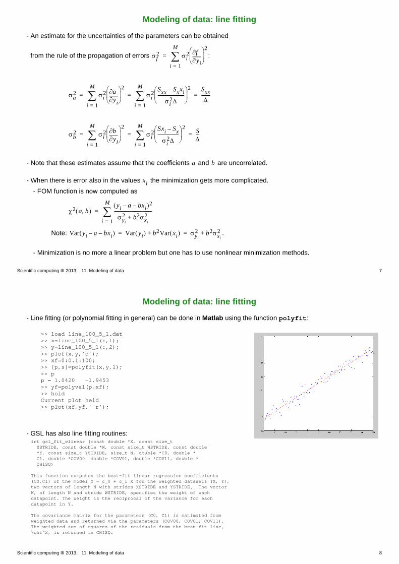
- Line fitting (or polynomial fitting in general) can be done in Matlab using the function polyfit:

>> load line_100_5_1.dat>> x=line_100_5_1(:,1);>> y=line_100_5_1(:,2);>> plot(x,y,’o’);>> xf=0:0.1:100;>> [p,s]=polyfit(x,y,1);>> pp = 1.0420 -1.9453>> yf=polyval(p,xf);>> holdCurrent plot held>> plot(xf,yf,’-r’);

- GSL has also line fitting routines:int gsl_fit_wlinear (const double *X, const size_t XSTRIDE, const double *W, const size_t WSTRIDE, const double *Y, const size_t YSTRIDE, size_t N, double *C0, double * C1, double *COV00, double *COV01, double *COV11, double * CHISQ)

This function computes the best-fit linear regression coefficients(C0,C1) of the model Y = c_0 + c_1 X for the weighted datasets (X, Y),two vectors of length N with strides XSTRIDE and YSTRIDE. The vectorW, of length N and stride WSTRIDE, specifies the weight of eachdatapoint. The weight is the reciprocal of the variance for eachdatapoint in Y.

The covariance matrix for the parameters (C0, C1) is estimated fromweighted data and returned via the parameters (COV00, COV01, COV11).The weighted sum of squares of the residuals from the best-fit line,\chi^2, is returned in CHISQ.


Modeling of data: general linear fitting

• Now the linearity means linearity of the model with respect to parameters .

- In general this can be expressed as

,

where are arbitrary functions or basis functions. Note that they need not be linear in .

- Our objective is to determine parameters in such a way that the basis functions reproduce the data as accurately as possible:

- Defining an matrix as , denoting with vector the parameters , and with vector the data

values we can express the least squares problem in matrix for as

.- Because this is an overdetermined system (more equations than unknowns, ) the equality should be understood in

the least squares sense; or ,

meaning that the norm of the residual is minimized:

- The most convenient norm in this case is the Euclidean norm i.e. .

ai

y x( ) akXk x( )k 1=

N=

Xk x( ) x

ai

yi Xk xi( )akk 1=

N

M N A Aij Xj xi= a N ai y M

yiAa y=

M N

Aa y

mina Aa y– p 2



- Actually the overdetermined problem may be more general than the one mentioned above.- An example1:

A surveyor measures heights of mountains.Measurement results are , , , , , .

We must compute the best estimates of the heights , , .- We can write down the equations

;

in matrix form:

h1

h2 h3

d21 d31

d23

Solution by Matlab

>> A=[1 0 0; 0 1 0; 0 0 1; -1 1 0; -1 0 1; 0 1 -1];>> b=[310 520 405 205 120 100]’;x=A\bx = 305 515 415

>> A*x-bans = -5 -5 9.99999999999994 5 -10.0000000000001 5.6843418860808e-14

h1 h2 h3 d21 d31 d23x1 x2 x3

x1 h1=

x2 h2=

x3 h3=

x1– x2+ d21=

x1– x3+ d31=

x2 x3– d23=

1 0 00 1 00 0 11– 1 01– 0 1

0 1 1–

x1x2x3

h1h2h3d21d31d23

=



- A simple example of a linear least squares problem is a polynomial of degree as basis functions:

.

- The FOM function is now

.

- This is more easily handled by the matrix notation:

is an matrix with elements

1. From M.T.Heath, Scientific Computing: An Introductory Survey, McGraw-Hill, 2002.

N

Xk x xk 1–=

2yi akXk xi( )

k 1=N–

i--------------------------------------------------

2

i 1=

M=

A M N AijXj xi( )

i-------------=



- Normally has more rows than columns ( ):

- Vector with elements is defined as

.

- Parameters are denoted by vector with elements.

- By setting the partial derivatives with respect to parameters to zero we get the equations

, .

A M N

X1 x1( )

1---------------

X2 x1( )

1---------------

X3 x1( )

1---------------

XN x1( )

1----------------

X1 x2( )

2---------------

X2 x2( )

2---------------

X3 x2( )

2---------------

XN x2( )

2----------------

X1 x3( )

3---------------

X2 x3( )

3---------------

X3 x3( )

3---------------

XN x3( )

3----------------

X1 xM( )

M----------------

X2 xM( )

M----------------

X3 xM( )

M----------------

XN xM( )

M-----------------

basis functions

data

poi

nts

b M

biyi

i-----=

ai a N

1

i2

------ yi ajXj xi( )j 1=

N– Xk xi( )

i 1=

M0= k 1 N=



- This can be written in the form

,

where

(or ), is an matrix and

(or ), is a vector with elements.

- Or in matrix form these normal equations are

or

.

- This group of equations can be solved using the normal linear algebra methods (LU and back substitution).

kjajj 1=

N

k=

kjXj xi( )Xk xi( )

i2

----------------------------i 1=

M= ATA= N N

kyiXk xi( )

i2

-------------------i 1=

M= ATb= N

a =

ATA a ATb=



- Let’s denote the inverse matrix as .

- To estimate the uncertainties of the parameters we can write the parameter as

.

- The estimated variance of can be found as in the case of line fitting

.

- Because is independent of

.

C 1–=

aj

aj jk1–

kk 1=

NCjk

yiXk xi

i2

--------------------i 1=

M

k 1=

N= =

aj

2 aj i2 aj

yi-------

2

i 1=

M=

jk yi

ajyi

-------CjkXk xi

i2

------------------------k 1=

N=



- Finally we get

..

- The term in the brackets is and we obtain

.

- One can also show that the off-diagonal elements of the matrix are the covariances of the parameters1.

- Sometimes the matrix is (nearly) singular. - In these cases we can not use the normal methods for solving the equation equations2.

- Moreover, the normal equations have as the multiplying matrix. One can show that the condition number of behaves as

.

(Remember that the condition number gives the error sensitivity of the linear problem

and .)

1. See e.g. Numerical Recipes, paragraph 15.6

2. In this case—when the matrix is symmetric positive definite—the Cholesky factorization , where is a lower triangular matrix.

2 aj CjkCjlXk xi Xl xi

i2

------------------------------i 1=

M

l 1=

N

k 1=

N=

kl Ckl1–=

2 aj Cjj=

C

A LLT= L

ATA

ATA A 2=

Ax b=x

x----------- A A

A------------ A A 1– A=



- A simple example:

, .

- For (with the machine epsilon ) we obtain for matrix

,

which is singular.

A1 1

00

= ATA 1 2+ 11 1 2+

=

0 1 2+ 1

A 1 11 1

=



- Moreover, the condition number of matrices and are as below:

, when .

, when .

A ATA

A1 1

00

= A+ 12 2+

--------------- 1 1 + 1–1 1– 1 +

=

A 2 2 2+= A+2

1---=

A A 2 A+2

2 2+------------------- 2-------= = 0

B ATA 1 2+ 11 1 2+

= B+ 12 2 2+

-------------------------- 1 2+ 1–1– 1 2+

=

B 2 2 2+= B+2

12

-----=

B B 2 B+2

2 2+2

--------------- 22

-----= = 0



- Here we have used (an matrix) which is so called pseudo-inverse of .- It is a generalization of matrix inverse for nonsquare matrices.- It has the following properties:

(i) (ii)

(iii)

(iv) .

- It is also the unique minimal norm solution to the problem

.

- Pseudo-inverse can be calculated using the singular value decomposition of matrix :

,

,

, ,

where are the singular values of (see below).

A+ N M A

AA+A A=

A+AA+ A+=

AA+ T AA+=

A+A T A+A=

minX RN M AX 1– F

A

A USVT=

A+ VS+UT=

S+ diag 11

------ 12

------ 1r

----- 0 0 RN M= r rank A=

i A



- We can transform the least squares problem to a more stable form by QR decomposition:

, where is an orthogonal matrix (i.e. ) and is an triangular matrix.

- As a figure:

- The least squares problem is now

.

- Now matrix is orthogonal, i.e. multiplying by it preserves the norm: .- Thus, the following equation is equivalent with the original one:

.

A Q R0

= Q M M QTQ 1= R N N

= *

A Q R

M

N M

M0

NN

Q R0

x b

Q Qv 22 Qv TQv vTQTQv vTv v 2

2= = = =

QTQ R0

x QTb R0

x QTb



- Because of the triangular form of matrix we can decompose the right hand side as , where is an -

vector and an -vector. The main point is that does not depend on .

- The equation is now .

- The residual norm becomes now:

.

- Because does not depend on we obtain the minimum by putting the first term to zero:

.

- The minimum norm is .

- In practice the QR decomposition is done by orthogonal transformations like Housholder reflections to columns of :.

- The right hand size is transformed accordingly:

R0

bc1c2

c1 N

c2 M N– c2 x

R0

xc1c2

b Ax– 22 c1

c2

R0

x–2

2

c1 Rx– 22 c2 2

2+= =

c2 x

Rx c1=

c2 22

AHNHN 1– H2H1A R=

HNHN 1– H2H1bc1c2

=



- Geometrical interpretation of the linear least squares problem in 3D/2D:

original equation or

- The vector produced from transform spans a subspace of (a plane; easily demonstrated with Matlab).- The range of matrix is defined as the space spanned by the column vectors of or

.

Ax ba11 a12a21 a22a31 a32

x1x2

b1b2b3

Ax R3

A A

ran A y R3 y; Ax= x R2;=

ran A

b

y Ax=

r b Ax–=Note that because:

,

and the normal equation tells us that

y r

Ax T b Ax– Ax Tb Ax TAx–xTATb xTATAx–

==

ATA x ATb=

Ax T b Ax– 0=

cosy 2b 2

----------=

One can show that the error in the solution behaves as

.x 2

x 2-------------- A

cos------------

b 2b 2

--------------



- A Matlab example1: water pumped through a container where dye is added. Concentration of dye as a function of time is measured. (blue curve). A second order polynomial is fitted to the data (red curve).

1. Data from example 6.4 in Kahaner, Moler, Nash: Numerical Methods and Software.



Original data: 1.0000 4.0225 2.0000 6.3095 3.0000 5.3522 4.0000 4.3553 5.0000 3.7861 6.0000 2.2947 7.0000 2.9492 8.0000 2.1732 9.0000 1.4921 10.0000 3.3424 11.0000 1.2596 12.0000 2.4732

Create the matrix A:A=[t.^0 t.^1 t.^2]A = 1 1 1 1 2 4 1 3 9 1 4 16 1 5 25 1 6 36 1 7 49 1 8 64 1 9 81 1 10 100 1 11 121 1 12 144

QR decomposition of A:[R,c]=qrsteps(A,b)R = -3.4641 -22.5167 -187.6388 0 11.9583 155.4574 0 0 36.5331 0 0 0 0 0 0 0 0 0 0 0 0 0 0 0 0 0 0 0 0 0 0 0 0 0 0 0c = -11.4922 -3.9747 0.9072 0.3239 0.2059 -0.8364 0.2649 -0.0664 -0.3049 1.9857 0.3411 1.9906

Solve the equation:y=R\cy = 6.2312 -0.6552 0.0248

Residual (original):A*y-bans = 1.5783 -1.2894 -0.8631 -0.3476 -0.2101 0.8993 -0.0876 0.4057 0.8537 -1.1799 0.7691 -0.5285

Residual (transformed):R*y - cans = 0.0000 0.0000 0.0000 -0.3239 -0.2059 0.8364 -0.2649 0.0664 0.3049 -1.9857 -0.3411 -1.9906

Matlab function qrsteps obtained from Cleve Moler: Numerical Comput-ing with Matlab, http://www.mathworks.com/moler/chapters.html



- When the problem is ill-conditioned singular value decomposition of the matrix may be of help.- SVD of an matrix ( 1) has the form

(or sometimes expressed in equivalent form )

where and are orthogonal ( is , is ): , ,

,

and

( ).

- Moreover, . are the singular values of .

- The smallest singular value is the distance (in the 2-norm) from to the nearest degenerate (singular) matrix.

- The number of non-zero ‘s is equal to the rank of the matrix. (Rank of an matrix is the dimension of its range. Range of a is the set of all -vectors where is an -vector.)

1. This is not required for a SVD to exist. In least squares, however, we always have more equations than variables.

AM N A M N

A USVT= UTAV S=

U V U M M V N N

UTU UUT 1M= = VVT VTV 1N= =

U u1 u2 uM= V v1 v2 vN=

S

1 0

2

0 N 0

= M N

1 2 N 0 i A

N A

M N A AM Ax x N



- If is singular then at least .

- SVD can tell many things about the matrix; assume we have, for matrix , ;

i.e. all singular values from are zero.- Then one can show that

- Various norm properties are related to SVD:

.

- Matrix can be expressed as a SVD expansion:

- In many cases is not exactly singular but almost. - In this case some of the singular values are small. - The ratio is a similar measure of the singularity of the matrix as the condition number.

A N 0=

A 1 2 r r 1+ N 0= = =

r 1+

(In some books .)ran A y RM y; Ax= x RN;=

range

rank A dim ran A=

null A x RN Ax; 0==

rank A r=null A span vr 1+ vr 2+ vN=

ran A span u1 u2 ur=

A F2

i2

i 1=

p= p min M N=

A 2 1=

minx 0Ax 2x 2

--------------- N= M N

A

A iuiviT

i 1=

r=

A

1 N



- To express this near rank-deficiency exactly the concept of -rank can be used

- If we define

, where ,

then one can prove that.

- Also, one can show that if then

, .

- With SVD one can define so called pseudo-inverse :,

, .

- Now the LS solution of the equation can be expressed as .

- is the solution for the minimization problem .

rank A min A B– 2rank B=

Ak iuiviT

i 1=

k= k r rank A=

minrank B k= A B– 2 A Ak– 2 k 1+= =

r rank A=

1 2 r r 1+ p p min M N=

A+

A+ VS+UT=

S+

1 1 0

1 2

0 1 r 0

RN M= r rank A=

Ax b= xLS A+b=

A+ minX RN M AX 1M– F



- SVD can be written in vector form as below

, or

.

- Compare these with the eigenvalue problem

.

- SVD is the “eigenvalue problem of nonsquared matrices”.

AV US= Avi iui=

ATU VST= ATui ivi=

Axi ixi=



- How is all this related to linear fitting?

- Well, first change the notation sligthly (Bear with me!):

Our data is ,

Basis functions are ,

Parameters are ,

So, the approximation we seek is .

In matrix form , where .

- In other words we have a minimization problem: we have to find

or we have to minimize the residual.

ti bi i 1 M=

j ti j 1 N=

xj j 1 N=

bi x1 1 ti x2 2 ti xN N ti+ + +

b Ax Aij j ti=

minx b Ax– 22 minx b Ax– i

2

i 1=

M=



- This norm can be written in terms of SVD of as (remember is orthogonal)

- If we denote

, we get

.

- If none of the singular values is zero we can get the minimum of the above norm by setting

.

A U

Ax b– 2 USVTx b– 2 UT USVTx b– 2 SVTx UTb– 2= = =

d UTb= z VTx=

Ax b– 22 Sz d– 2

2

1z1 d1–

2z2 d2–

NzN dN–

dN 1+–

dN 2+–

dM–2

2

1z1 d1– 2NzN dN– 2 dN 1+

2 dM2+ + + + += = =

zidi

i-----=



- This gives the norm its minimum value

.

- If then any choice of gives the same minimum residual

.

- This means that the least squares problem doesn’t have a unique solution.

- Usual convention is to set whenever .

- Singular values are nonzero only if the basis functions are linearly independent. - Near linear dependence between basis functions implies a singular value close to zero.

- Thresholds for the singular values can be used as the tolerance of the fit.- Any greater than the threshold is acceptable and the corresponding parameter value

is computed from .

- Any smaller than the threshold value is deemed as negligible and it set to zero.

- The only drawback of the SVD method is that it is slower than solving the normal equations.

Ax b– 22 dN 1+

2 dM2+ +=

N 0= zN

Ax b– 22 dN

2 dN 1+2 dM

2+ + +=

zi 0= i 0=

i

izi di i=

i



• SVD has many other applications. See any textbook on numerical methods.

• SVD can be calculated by

Matlab: [U,S,V]=svd(A);

LAPACK: SUBROUTINE DGESVD(JOBU,JOBVT,M,N,A,LDA,S,U,LDU,VT,LDVT,WORK,LWORK,INFO)

GSL: int gsl_linalg_SV_decomp(gsl_matrix *A, gsl_matrix *V, gsl_vector *S, gsl_vector *WORK)


Modeling of data: nonlinear fitting

• Now we generalize the fitting problem to models where the dependence on the parameters is nonlinear.

• Due to nonlinearity in minimizing the we have to resort to iterative methods.

- As in function minimization in general, we start with a initial guess for the parameter vector and by using

our algorithm proceed in the parameter space until the minimum of has been reached.

- Following the principles developed in Chapter 8 the function can be approximated as quadratic near the minimum

,

where is a vector with elements and is an matrix.

- Minimum of this function is found with one single step

.

- If the function is not well approximated by a quadratic function we can use e.g. the steepest descent direction

,

where the constant is small enough not to start going uphill.

aj

2

a1 a2 aN2

2 a( ) dTa– 12--- aTDa+

d N D N N

a i 1+ a i D 1– 2 a i( )–+=

2

a i 1+ a i 2 a i( )–=



- The difference between minimization in fitting and function minimization in general is that now we are able to compute both the gradient and the Hessian matrix. (We built the model, didn’t we!)

- Our model is ,

where the dependence of on is no more linear.

- FOM function is now

- Components of the gradient are

, .

- Elements of the Hessian matrix are

.

y y x a;( )=y a

2 a( )yi y xi a;( )–

i--------------------------

2

i 1=

M=

2 a( )

2

ak--------- 2

yi y xi a;( )–

i2

--------------------------y xi a;( )

ak-------------------

i 1=

M–= k 1 2 N=

Dkl2 2

ak al----------------- 2 1

i2

------y xi a;( )

ak-------------------

y xi a;( )al

------------------- yi y xi a;( )–2y xi a;( )ak al

----------------------–i 1=

M= =



- Let’s drop those 2’s by defining

, .

so that

.

- Now the iteration equation can be written in the form

. (1)

where is the movement in one iteration step.

- From equation (1) we solve and add it to the current position, thus giving us the new point.

- The steepest decent step takes the form

. (2)

k12---

2

ak---------–= kl

12---

2 2

ak al-----------------=

12---D=

a i 1+ a i D 1– 2 a i( )–+=

kl all 1=

N

k=

al ali 1+ al

i–=

al

al l=



- Hessian matrix contains the second derivatives of with respect to the parameters . - In most algorithms these terms are dropped.

- This can be justified by observing that the coefficient of the term is which is essentially (for a successful model) the randomly distributed error of the data.

- Because of this we can assume that these terms more or less cancel out each other. - In case of outliers keeping the second derivatives can make the algorithm unstable.

- So, we redefine matrix :

.

- Changing this way does not change the end results; only the route in the space that takes us to the minimum is changed.

- Note that dropping those second derivatives from the Hessian results in also by assuming that the model is linear in .

2 ai

2y ak al yi y xi( )–

kl 2 1

i2

------y xi a;( )

ak-------------------

y xi a;( )al

-------------------i 1=

M=

a

y y x a;( )=a



- In the Levenberg and Marquardt (LM) method the steepest descent is used when far away from the minimum- When the minimum of the is approached the method gradually shifts to the (approximate) inverse Hessian method.

- The value of the constant in equation (2) is estimated by the Hessian matrix:- Dimension of is .

- The only element in the Hessian matrix with this dimension is . - Let’s assume that this element tells us the ‘scale’ of the problem. - Moreover, in oder not to do too long jumps we divide it by a number .- So we get the equation (2) to form

. (3)

- Combining the inverse Hessian and SD methods goes like this:

- Let’s define the matrix :

.

- Replace equations (1) and (3) by one equation

. (4)

2

ak2

1 kk

1»

al1

ll---------- l=

''jj jj 1 +=

'jk jk= j k

'kl all 1=

N

k=



- If is large equation (4) approaches equation (3) while for small we obtain the Hessian equation (1)

- The LM algorithm is then the following (the initial parameter vector is )

1. Compute 2. Set a small value to . E.g. .3. Solve from equation (4) and compute .

4. If , increase ( ) and go to step 3.5. If decrease : , update vector and go to step 3.

- We also need a condition for stopping the iteration.- In practice stopping after decreases only slightly (say 0.01) is a good measure of convergence.

- After convergence the error estimates of the parameters can be computed from .

a

2 a( )0.001=

a 2 a a+( )2 a a+( ) 2 a( ) 102 a a+( ) 2 a( ) 10 a a a+

2

C 1–=



- As an example below are the fits of Maxwell-Boltzmann distribution

to the data obtained from the molecular dynamics simulation of solid Lennard-Jones (in this case Ne) material.

y ax2e x2 2b–=

vdfit> ../fitf/fitf vd70.dat boltzmann-------------------------- fitf ---------------------------Fitting function boltzmann to experimental file vd70.dat y=a*x**2*exp(-x**2/2.0/b)

> fitfunc vd70.dat 2 1 1

a b CHI^2 Lambda ------------ ------------ ------------ ------------ 1.0000000 1.0000000 0.16260163E-02 0.10000000E-02 10.551674 5.1415530 19498.413 1000.0000 10.550628 5.1404933 19498.392 100.00000 10.540944 5.1300143 19498.190 10.000000 10.509482 5.0350311 19496.523 1.0000000 12.569750 4.3980820 19487.114 0.10000000 19.954605 3.8127834 19471.618 0.10000000 41.200786 3.2570494 19434.872 0.10000000 111.62496 2.7146669 19334.445 0.10000000 428.58148 2.1554226 18994.058 0.10000000 2671.5811 1.5655949 17473.904 0.10000000 17594.094 1.5383770 9299.2787 0.10000000 48717.769 0.98988380 4880.1334 0.10000000E-01 88756.809 1.0996447 193.74644 0.10000000E-02 89438.680 1.0468608 2.1225936 0.10000000E-03 89969.741 1.0425107 1.6102341 0.10000000E-04 89974.933 1.0424922 1.6102060 0.10000000E-05 89974.941 1.0424922 1.6102060 0.10000000E-06

sigmaa sigmab CHI^2(ABS) ----------- ----------- ------------ 41.107902 0.24614145E-03 990.27666



- Implementations of the LM algorithm:

GSL: Derivative Solver: gsl_multifit_fdfsolver_lmsder This is a robust and efficient version of the Levenberg-Marquardt

algorithm as implemented in the scaled LMDER routine in MINPACK. Minpack was written by Jorge J. More’, Burton S. Garbow and Kenneth E. Hillstrom

Matlab: X=LSQCURVEFIT(FUN,X0,XDATA,YDATA) starts at X0 and finds coefficients X to best fit the nonlinear functions in FUN to the data YDATA (in the least-squares sense).

SLATEC: DNLS1E: The purpose of the routine is to minimize thesum of the squares of M nonlinear functions in N variables by a modification of the Levenberg-Marquardt algorithm.

- SLATEC is a collection of Fortran (F77!) routines doing various kinds of numerical tasks.- It can be downloaded from www.netlib.org or www.csit.fsu.edu/~burkardt/f_src/slatec/slatec.html.- If you download it from the latter place you need also the F90 f90split program to split the one big file to separate

subroutines (http://www.csit.fsu.edu/~burkardt/f_src/f90split/f90split.html).- Using the scripts you can create a library (.a file) that can be linked with your main program.



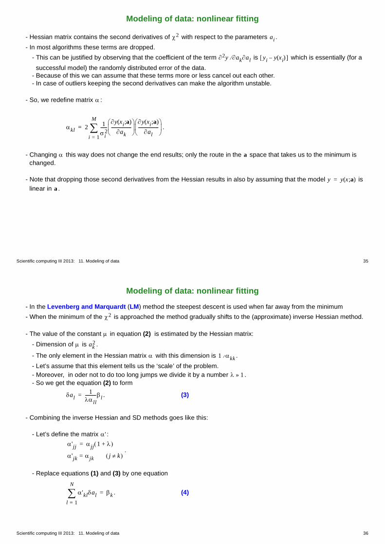
- Matlab Curve Fitting Toolbox is a nice tool for nonlinear fitting.

- Example: In order to obtain a measure of a width of a stretched cylindrical SiO2 beam fit a modified Fermi function to the atomic density as a function of distance from the center line if the beam:

.

(This width is in turn used to calculate the Poisson’s ratio of the beam: .)

r

n r

r

x

z

n r a br–e r c– d 1+-------------------------------=

x z–=



- Below is listed the Matlab script doing the fit and the results.%% Script fits a modified Fermi function%% a-b*r% d(r) = ----------------% exp((r-c)/d)+1%% to the radial distributions of atoms in a cylindrical beam.%% Antti Kuronen, 2009, [email protected]%

n0=10;g=fittype('(a-b*x)/(exp((x-c)/d)+1)','coeff',{'a','b','c','d'});d=load('dist.dat');[fp,gof,output]=...fit(d(n0:end,1),d(n0:end,2),g,'Startpoint',[5 0.1 60 1]);fprintf('a %g b %g c %g d %g\n',fp.a,fp.b,fp.c,fp.d);

h=figure;hold on;

h1=plot(d(:,1),d(:,2),'b.'); set(h1,'Marker','o');set(h1,'MarkerSize',4);set(h1,'MarkerFaceColor','blue');

h2=plot(fp);set(h2,'LineWidth',2.0)legend off;

ha=gca;set(ha,'FontSize',14);set(get(ha,'XLabel'),'String','{\it r} (Å)','FontSize',14);set(get(ha,'YLabel'),'String','{\it n} ({\it r})','FontSize',14)

>> fitmla 4.44564 b 9.88383e-05 c 61.2408 d 0.398287


Modeling of data: parameter errors

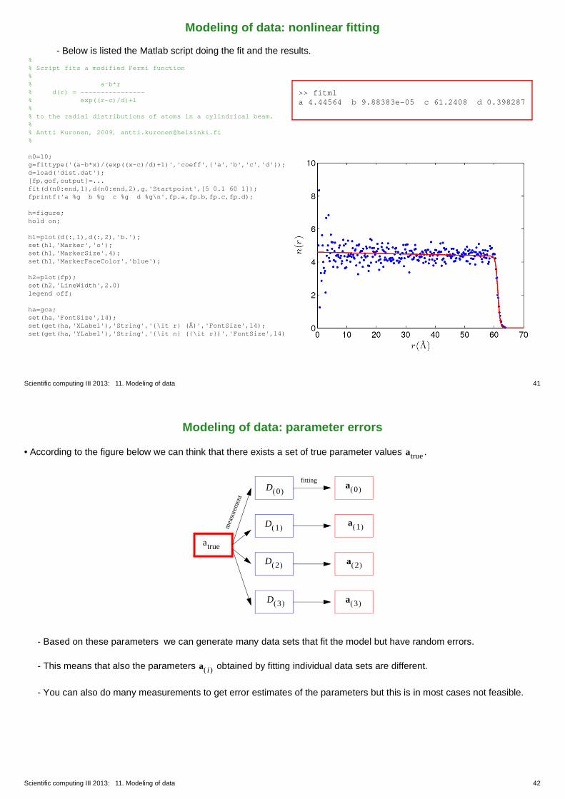
• According to the figure below we can think that there exists a set of true parameter values .

- Based on these parameters we can generate many data sets that fit the model but have random errors.

- This means that also the parameters obtained by fitting individual data sets are different.

- You can also do many measurements to get error estimates of the parameters but this is in most cases not feasible.

atrue

mea

sure

men

t

fitting

atrue

D 0

D 1

D 2

D 3

a 0

a 1

a 2

a 3

a i



- What you can do is generate artificial data sets by using Monte Carlo: this is called the bootstrap method:

- Note that we must know the distribution of the errors in the data points in order to generate the data.

measureddata

fitting

fittingMC-simulation

a0

D 0s

D 1s

D 2s

D 3s

a 0s

a 1s

a 2s

a 3s

distribution of

parameters



• We can also use the function as a basis for the error estimation.

- Confidence limits for the parameters can be com-puted as constant- boundaries.

- Assume that the has the distribution with

degrees of freedom. With a reasonable fit one can show that the parameters are normally distrib-uted:

.

- Moreover, the quantity is

distributed as a distribution with degrees of freedom. Here

is the true parameter vector and one realization of it.

- Confidence region of one parameter can be expressed in terms of

the matrix as

,

where is now the change in that defines the confidence level.- In the case of fitting by using SVD the elements of the matrix are simply obtained as

, where is now the th singular value.

- For determining joint confidence regions for more than one parameter see e.g. Numerical Recipes.

a2

a1

min2

min2

12+

min2

22+

a2

2 a

2

min2 2

M N–

P a 12---– a T aexp

From Numerical Recipes.

2 2 a j2 atrue–=

2 M atruea j

ai

C 1–=

ai2 Cii=

2 2

C

Cjk VjiVki i2

i 1=N= i i


Modeling of data: data smoothing

• Data smoothing can be done by various means.

- By fitting a polynomial to the data set. Of course, the degree of the polynomial must be lower than the number of data points.

- By constructing a spline that has a restricted ‘bending energy’ (average curvature) but nonetheless goes near the data points. This can be accomplished by minimizing the following quantity

,

where is the good old chi-squared and the last term gives the approximate average curvature.- Parameter controls the relative weight of the two terms:

with we get a straight linewith we get a normal spline interpolant.

W 2 S'' x 2 xd+=

2

0=


Modeling of data: robust estimation

• In robust estimation we aim to diminish the effect of outlier points to the result of the fit. - It might be that we know that the distribution of our data comprises of a

narrow peak and a broad tail of outliers.- The idea in robust estimation is to write the probability distribution not

as

but

.

- In fitting we then want to minimize

.

- Often the argument of is of the form .

- Defining we get the minimization equations as

, .

Numerical Recipes, Fig. 15.7.1

P 12---

yi y xi a( )–

i---------------------------

2–exp y

i 1=

M

P yi y xi a–exp yi 1=

M

yi y xi ai 1=

M

zyi y xi a–

i----------------------------

z d zdz

--------------=

1i

-----yi y xi a–

i----------------------------

y xi aak

---------------------i 1=

M0= k 1 N=


Modeling of data: robust estimation

- For normal distribution we get

, .

- If we have errors distributed as double exponential

we get , .

- Sometimes a Lorentzian distribution is appropriate:

,

which gives

, .

z 12---z2= z z=

Pyi y xi a( )–

i---------------------------–exp y

i 1=

M

z z= z sign z=

P 1

1 12---

yi y xi a–

i----------------------------

2+

-------------------------------------------------- yi 1=

M

z 1 z2 2+ln= z z1 z2 2+---------------------=

modeling of data - acclab.helsinki.fi · modeling of data 1 modeling of data the problem is roughly...

Documents