Modeling Multivariate Processes on the Unit Simplex

Tano SantosColumbia University and NBER

Pietro VeronesiUniversity of Chicago, NBER and CEPR

This note discusses some common questions that we received about the “share process”introduced in Menzly Santos and Veronesi (2004), and discusses its properties. The mainreferences are Menzly, Santos and Veronesi, “Understanding Predictability,” JPE, 2004, andSantos and Veronesi “Labor Income and Predictable Returns,” RFS, forthcoming.

First, the process in its general form can be written as a multivariate, continuous timeVector Autoregressive (VAR) process

dst = Λ′·stdt + I (st)(v − 1n × s′t · v

) · dBt (1)

where I (st) is a diagonal matrix with sit on its ii-th element, Bt is a (N × 1) vector Brownian

motion, Λ is a n × n matrix descibed below,

st =

⎛⎜⎝

s1t...

snt

⎞⎟⎠ ; v =

⎡⎢⎣

v1

...vn

⎤⎥⎦

wherevi =

(vi1, ..., v

iN

)and 1n is a vector of ones. For instance, the share i follows the process

dsit =

⎛⎝ n∑

j=1

sjtλji

⎞⎠ dt + si

t

(vi−s′t · v

) · dBt (2)

This process is formally identical to a belief process in a continuous time, regime switch-ing model, where Λ is the instantaneous “transition matrix” (infinitesimal generator). Ageneral treatment of such processes, including existence and properties, is contained in Liptserand Shyriaev (1977), Chapter 9. Veronesi (2000, JF) adopts this methodology in his learningmodel. In what follows, we provide simple implications.

Point 1: Note that if at time t we have∑n

i=1 sit = 1, then the diffusion of the sum of

sit, St =

∑ni=1 si

t, is equal to zero. In fact

Diffusion(dSt) = σS =n∑

i=1

sit

(vi−s′t · v

) · dBt

1

=

{s′t · v−

(n∑

i=1

sit

)s′t · v

}· dBt

={s′t · v − s′t · v

} · dBt= 0

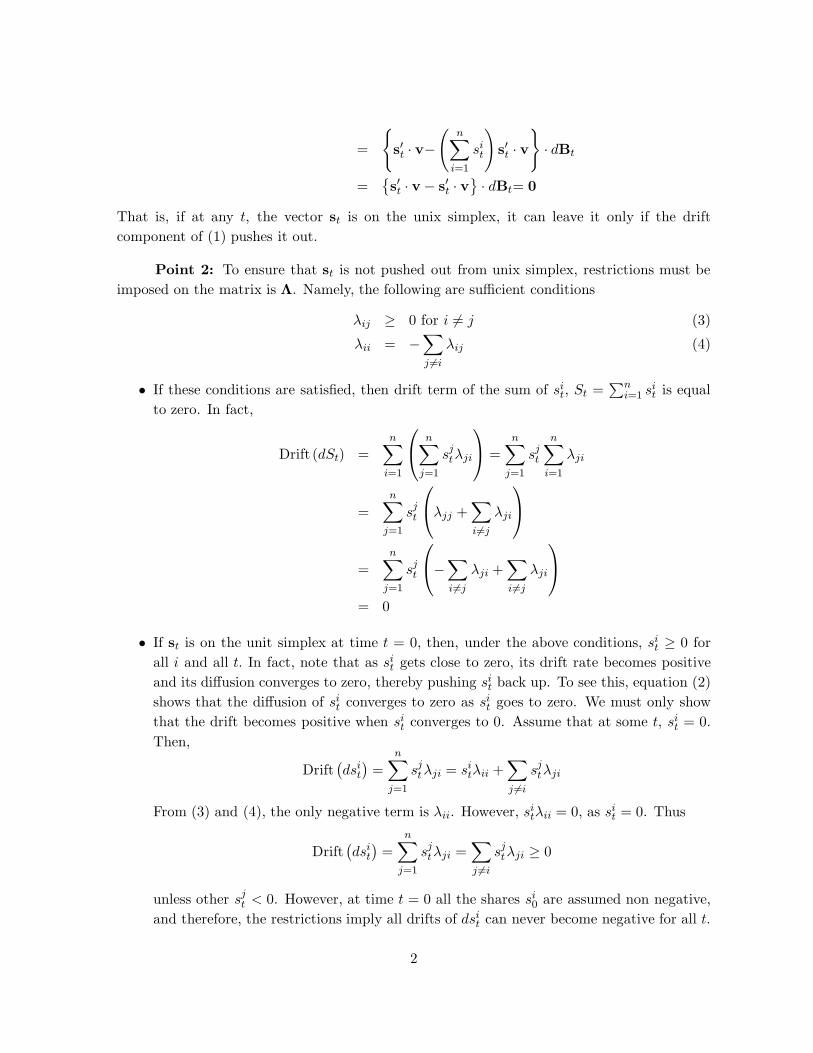
That is, if at any t, the vector st is on the unix simplex, it can leave it only if the driftcomponent of (1) pushes it out.

Point 2: To ensure that st is not pushed out from unix simplex, restrictions must beimposed on the matrix is Λ. Namely, the following are sufficient conditions

λij ≥ 0 for i �= j (3)

λii = −∑j �=i

λij (4)

• If these conditions are satisfied, then drift term of the sum of sit, St =

∑ni=1 si

t is equalto zero. In fact,

Drift (dSt) =n∑

i=1

⎛⎝ n∑

j=1

sjtλji

⎞⎠ =

n∑j=1

sjt

n∑i=1

λji

=n∑

j=1

sjt

⎛⎝λjj +

∑i�=j

λji

⎞⎠

=n∑

j=1

sjt

⎛⎝−

∑i�=j

λji +∑i�=j

λji

⎞⎠

= 0

• If st is on the unit simplex at time t = 0, then, under the above conditions, sit ≥ 0 for

all i and all t. In fact, note that as sit gets close to zero, its drift rate becomes positive

and its diffusion converges to zero, thereby pushing sit back up. To see this, equation (2)

shows that the diffusion of sit converges to zero as si

t goes to zero. We must only showthat the drift becomes positive when si

t converges to 0. Assume that at some t, sit = 0.

Then,

Drift(dsi

t

)=

n∑j=1

sjtλji = si

tλii +∑j �=i

sjtλji

From (3) and (4), the only negative term is λii. However, sitλii = 0, as si

t = 0. Thus

Drift(dsi

t

)=

n∑j=1

sjtλji =

∑j �=i

sjtλji ≥ 0

unless other sjt < 0. However, at time t = 0 all the shares si

0 are assumed non negative,and therefore, the restrictions imply all drifts of dsi

t can never become negative for all t.

2

Point 3: Note that the diffusion term of (1) obtains in any model where the shareprocesses are endogenously derived from a primitive model of, say, cash flows, with constantvolatility. For instance, suppose that n assets (industries, countries, etc.) are assumed toproduce output according to the processes

dDit

Dit

= μi (Dt) dt + vdBt (5)

where μi (Dt) is the drift rate of output growth, which may depend on the vector Dt =(D1

t , .., Dnt

)of outputs. Define now

sit =

Dit∑n

j=1 Djt

the share of output produced by asset i over the total∑n

j=1 Djt . An application of Ito’s Lemma

shows

dsit = μi

s,tdt + sit

⎛⎝vi −

n∑j=1

sjtv

j

⎞⎠ dBt

That is, the diffusion term in (1) arises naturally from first principles. What differs isreally the drift rate, which (1) simplies into a linear VAR model, while the use of Ito’s Lemmawould imply some non-linear term as well.

Examples:

1. Menzly, Santos and Veronesi (JPE, 2004): Let there be n financial assets paying adividend stream Di

t. Denote sit = Di

t/Yt, where Yt = wt +∑n

i=1 Dit is the total income

available for consumption. Here wt represent the amount of income that is not financialin nature. Assume each dividend share si

t, for i = 1, ..., n, follows the process

dsit = φi

(si − si

t

)dt + si

t

⎛⎝vi −

n∑j=0

sjtv

j

⎞⎠ dBt (6)

Let

swt = s0

t = 1 −n∑

i=1

sit

be the consumption that springs from sources other than financial assets. In order toensure that sw

t ≥ 0 for all t, we must impose a restriction on the drift rates of shares sit,

for i = 1, ..., n. The following is a sufficient condition (see MSV(2004, page 8)):

φi ≥n∑

j=1

φjsj. (7)

3

It easy to verify that under this condition, the sufficient conditions (3) and (4) are alsosatisfied, thereby yielding the result that the vector st =

(s0t , ..., s

nt

)lies on the unit

simplex for all t.

2. Consider the specialization to φi = φj = φ. If all firms have the same speed of meanreversion, then also s0

t = 1 −∑ni=1 si

t follows the same process (6). In fact:

ds0t = −

n∑i=1

dsit = −

n∑i=1

φ(si − si

t

)dt −

n∑i=1

sit

⎛⎝vi −

n∑j=0

sjtv

j

⎞⎠ dBt

= φ(−Σn

i=1si + Σn

i=1sit

)dt −

⎛⎝ n∑

i=1

sitv

i −(

n∑i=1

sit

)n∑

j=0

sjtv

j

⎞⎠ dBt

= φ(s0 − s0

t

)dt −

⎛⎝ n∑

i=1

sitv

i − (1 − s0t

) n∑j=0

sjtv

j

⎞⎠ dBt

= φ(s0 − s0

t

)dt −

⎛⎝ n∑

i=1

sitv

i −n∑

j=0

sjtv

j + s0t

n∑j=0

sjtv

j

⎞⎠ dBt

= φ(s0 − s0

t

)dt −

⎛⎝−s0

t v0 + s0

t

n∑j=0

sjtv

j

⎞⎠ dBt

= φ(s0 − s0

t

)dt + s0

t

⎛⎝v0 −

n∑j=0

sjtv

j

⎞⎠ dBt

where we used(−Σn

i=1si + Σn

i=1sit

)=(1 − Σn

i=1si − 1 + Σn

i=1sit

)= s0 − s0

t . Note thefollowing:

• The volatility of labor share is multiplied by s0t , that is, the fact that s0

t > 0 in oursetting is implicitly assumed from the other assumptions about shares of financialassets.

• Even in the original processes (6), we have s0t showing up in the volatility term, as

the summation starts from 0 and not 1! This is key to keep s0t > 0.

• The process (6) is formally identical to the stochastic process that beliefs follow ina regime switching model with unobservable regimes, equal probability of shifting(= φ), and unconditional probability of the new regime given by the probabilitydistribution s. See Veronesi (2000, equation (5), page 5).

3. A numerical example: What happens if the condition on the drift is violated?

• Consider the following numerical example:

n = N = 2

4

v0 = [.01, .02]

v1 = [.03, .05]

v2 = [.08, .20]

s1 = s2 = .45

φ1 = .01

φ2 = .05

• Using these inputs, simulations show that s0t may become negative. To use the

words of a reader of MSV that pointed this example out to us:

“Using these values, we start s1 and s2 at their long run values of .45, implyingthat s0 starts at .10. We then used a simple Euler discretization of the SDEs using1,000 steps per year and simulated paths out for 100 years. Using different startingseeds, we simulated the paths of the shares 100 times. Of these 100 paths, 29 had aminimum value for s0

t less than zero. These minima ranged from about just slightlyless than zero to -.285. We increased the discretization precision, but still get thesame results”

• The answer to the puzzle: Condition (7) is violated. In fact, the above parametersimply

2∑j=1

sjφj = 0.0270 > φ1 = .01

• Figure 1 shows what happens when the condition is violated. The figure plots the surfaceof the drift rate of s0

t = 1−s1t −s2

t as a function of (s1t , s

2t ) in the space where s1

t +s2t ≤ 1.

This drift rate is given by

Drift(ds0t ) = −φ1(s1 − s1

t )− φ2(s2 − s2t )

• We also plot the zero plane. As it can be seen, under the parameters above, the driftrate of ds0

t is negative when (s1t , s

2t ) is around (1, 0) and s1

t + s2t = 1. This implies that s0

t

will be pulled down (or equivalently, s1t + s2

t will be pulled upwards), thereby violatingthe non-negativity of s0

t .

• Figure 2 shows the same plot but for a parametrization where the restriction is insteadsatisfied. This figure shows that the drift of ds0

t should be positive for all combinationswhere s1

t + s2t = 1, a situation violated by the previous parametrization.

• Simulations confirm this pattern. From the above parameters, there are two ways tomeet the restriction (7). The first is to increase φ1. The minimum φ1 that meets (7)is about φ1 = 0.041. The second is to pull down φ2. The maximum φ2 that meets

5

(7) is φ2 = 0.012. In both cases, simulations (of course) produce no violations of thenon-negativity constraint. (Interestingly, note that making s2

t less stationary makes theproblem go away: it is the interaction between the speed of mean reversion of the 2processes s1

t and s2t that matter for s0

t )

00.2

0.40.6

0.81

0

0.2

0.4

0.6

0.8

1−0.03

−0.02

−0.01

0

0.01

0.02

0.03

s1

Drift rate of s0: phi1=.01, phi2=.05

s2

drift o

f s0

Figure 1. The drift of s0t when condition (7) is violated.

6

00.2

0.40.6

0.81

0

0.2

0.4

0.6

0.8

1−10

−8

−6

−4

−2

0

2

x 10−3

s1

Drift rate of s0: phi1=.01, phi2=.011

s2

drift o

f s0

Figure 2. The drift of s0t when condition (7) is satisfied.

7