modeling linkages in r using linkr - aaron olsen linkages using... · modeling linkages in r using...

Modeling linkages in R using linkRSimulating two- and three-dimensional linkage mechanisms

using the R package ‘linkR’

0 10 20 30 40 50 60

0.0

0.2

0.4

0.6

0.8

1.0

i

Inpu

t dis

plac

emen

t

0 10 20 30 40 50 60

0.0

0.2

0.4

0.6

0.8

i

Out

put d

ispl

acem

ent

0 10 20 30 40 50 60

0.4

0.6

0.8

1.0

1.2

1.4

i

1 / f

MA

October 2016Version 1.1

Modeling linkages using linkR, v1.1 TABLE OF CONTENTS

Table of Contents1 Introduction 4

2 Getting started 5

3 Defining a linkage 73.1 Joint coordinates . . . . . . . . . . . . . . . . . . . . . . . . . . . . . . . 73.2 Joint types . . . . . . . . . . . . . . . . . . . . . . . . . . . . . . . . . . . 73.3 Joint constraint vectors . . . . . . . . . . . . . . . . . . . . . . . . . . . . 83.4 Joint connections . . . . . . . . . . . . . . . . . . . . . . . . . . . . . . . 93.5 Calling ‘defineLinkage’ . . . . . . . . . . . . . . . . . . . . . . . . . . . . 103.6 Adding associated points . . . . . . . . . . . . . . . . . . . . . . . . . . . 113.7 Connecting associated points into shapes . . . . . . . . . . . . . . . . . . 12

4 Simulating linkage motion 144.1 Calling ‘animateLinkage’ . . . . . . . . . . . . . . . . . . . . . . . . . . . 14

5 Analyzing linkage motion 185.1 Joint position over time . . . . . . . . . . . . . . . . . . . . . . . . . . . 185.2 Point position over time . . . . . . . . . . . . . . . . . . . . . . . . . . . 205.3 Calling ‘linkageKinematics’ . . . . . . . . . . . . . . . . . . . . . . . . . 215.4 Angular displacement and velocity of links . . . . . . . . . . . . . . . . . 225.5 Displacement and velocity of joints . . . . . . . . . . . . . . . . . . . . . 235.6 Displacement and velocity of points . . . . . . . . . . . . . . . . . . . . . 245.7 Torque mechanical advantage . . . . . . . . . . . . . . . . . . . . . . . . 255.8 Force mechanical advantage . . . . . . . . . . . . . . . . . . . . . . . . . 27

6 Examples 286.1 Planar 4-bar (RSSR) . . . . . . . . . . . . . . . . . . . . . . . . . . . . . 286.2 3D 4-bar (RSSR) . . . . . . . . . . . . . . . . . . . . . . . . . . . . . . . 296.3 Two coupled sliders (LSSL) . . . . . . . . . . . . . . . . . . . . . . . . . 306.4 Coupled planar and linear sliders (SSPSSL) . . . . . . . . . . . . . . . . 316.5 Three coupled sliders (LSSLSSL) . . . . . . . . . . . . . . . . . . . . . . 336.6 Crank-driving sliding link (RSSL) . . . . . . . . . . . . . . . . . . . . . . 346.7 Slider along rotating link (RLSS) . . . . . . . . . . . . . . . . . . . . . . 356.8 Rotating links in series (RRSS) . . . . . . . . . . . . . . . . . . . . . . . 366.9 Coupled linear, planar sliders (LSSLSSPSS) . . . . . . . . . . . . . . . . 386.10 Sliders coupled by rotating link (LSSRSSL) . . . . . . . . . . . . . . . . 396.11 Coupled rotating, linear links (RSSLSSR) . . . . . . . . . . . . . . . . . 406.12 Coupled rotating, planar links (RSSRSSPSS) . . . . . . . . . . . . . . . . 416.13 Two 3D 4-bars in series (RSSRSSR)) . . . . . . . . . . . . . . . . . . . . 426.14 Slider, 3D 4-bar in series (RSSR(SSL)) . . . . . . . . . . . . . . . . . . . 436.15 Slider, 2D 4-bar in series (R(SSL)SSR) . . . . . . . . . . . . . . . . . . . 446.16 Slider in parallel with 4-bar (RS(SSL)SR) . . . . . . . . . . . . . . . . . 456.17 Fish cranial joint configuration . . . . . . . . . . . . . . . . . . . . . . . 46

2

Modeling linkages using linkR, v1.1 TABLE OF CONTENTS

6.18 Bird cranial linkage . . . . . . . . . . . . . . . . . . . . . . . . . . . . . . 486.19 Fish cranial linkage . . . . . . . . . . . . . . . . . . . . . . . . . . . . . . 49

7 Citing linkR 52

8 Acknowledgements 52

3

Modeling linkages using linkR, v1.1 1 Introduction

1 IntroductionDuring my time as a graduate student I became fascinated by how differences in the in-ternal structure among animals relates to the different ways in which they move. I spentmuch of that time at the Field Museum of Natural History in Chicago, exploring theskeleton collections and observing the diverse ways in which animal bodies have evolved.There is a long and rich history of researchers using simple mechanical models to simulatethe motion of bones and joints in animals. Building off this work, I wanted to developmy own motion simulations using data collected from natural history specimens.

In particular, I wanted to model the motion of interconnected bones as mechanical link-ages (e.g. a 4-bar linkage), a type of analysis referred to in engineering as kinematic sim-ulation. There are a number of advanced software tools currently available for multibodysimulation and force analysis (e.g. Adams Multibody Dynamics, Abaqus, SimMechanics,SIMPACK MBS software, AnyBody Modeling System). However, these programs weremore expensive than I could afford and had capacities far exceeding those that I neededfor my linkage simulations. Additionally, I wanted the code that I used to be accessibleto anyone who wanted to replicate my results or create simulations of their own. Fromthis the linkR package was born.

Although linkR could have been developed using any basic programming language, I findR packages to be one of the easiest and standardized means of distributing software.Developing linkR on the R platform has the added advantage of integrating linkR withtwo other R packages I have developed over the past several years: StereoMorph andsvgViewR. StereoMorph provides one approach for collecting shape data that can beused to create linkage simulations while svgViewR provides an easy-to-use platform forvisualizing the resulting 3D, animated simulations.

This tutorial will take you through all the steps of using the linkR R package to simulate,analyze, and visualize the motion of basic linkage mechanisms. All of the required code isincluded within this tutorial so no separate files are required. The last section, Examples,provides commented code for creating many linkages of differing configurations. I hopeyou find this tutorial helpful and wish you the best with your project!

Aaron OlsenOctober 2016

4

https://aaronolsen.github.io/software/stereomorph.html

https://aaronolsen.github.io/software/svgviewr.html

Modeling linkages using linkR, v1.1 2 Getting started

2 Getting startedThis tutorial will show you how to create 2D and 3D linkage models using the R packagelinkR. The R project is a computing language and platform that allows users to freelyupload and share software packages. The linkR package includes functions for simulatingand analyzing the kinematics of 2D and 3D linkage mechanisms. The linkR package usesthe R package svgViewR to create 3D interactive animations that can visualized in theweb browser. The following steps will take you through process of installing the linkRpackage.

1. If you do not already have R installed on your computer, begin by installing R. R canbe installed on Windows, Linux and Mac OS X.

2. Once installed, open R.

3. Go to Packages & Data > Package Installer.

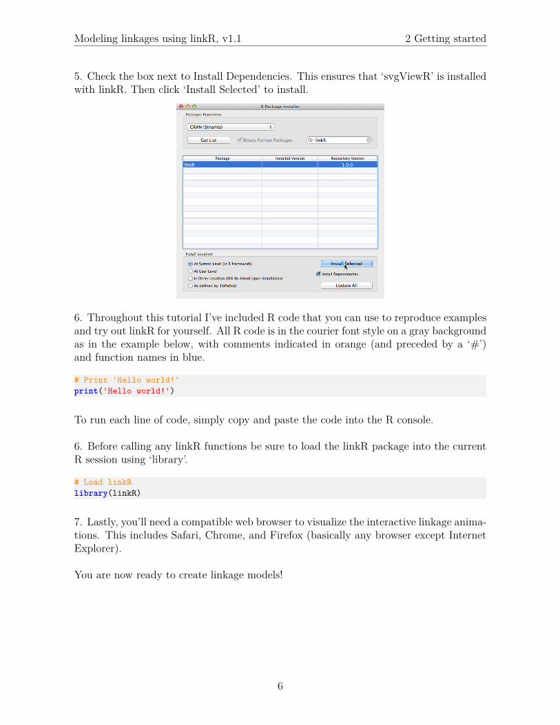
4. Find the linkR package binary by typing ‘linkR’ into the Package Search box andclicking Get List. (The repository version of linkR will differ from that in the version inthe image below).

5

http://cran.r-project.org/web/packages/linkR/index.html

http://cran.r-project.org/

http://cran.r-project.org/web/packages/svgViewR/index.html

http://cran.r-project.org/

Modeling linkages using linkR, v1.1 2 Getting started

5. Check the box next to Install Dependencies. This ensures that ‘svgViewR’ is installedwith linkR. Then click ‘Install Selected’ to install.

6. Throughout this tutorial I’ve included R code that you can use to reproduce examplesand try out linkR for yourself. All R code is in the courier font style on a gray backgroundas in the example below, with comments indicated in orange (and preceded by a ‘#’)and function names in blue.

# Print 'Hello world!'print('Hello world!')

To run each line of code, simply copy and paste the code into the R console.

6. Before calling any linkR functions be sure to load the linkR package into the currentR session using ‘library’.

# Load linkRlibrary(linkR)

7. Lastly, you’ll need a compatible web browser to visualize the interactive linkage anima-tions. This includes Safari, Chrome, and Firefox (basically any browser except InternetExplorer).

You are now ready to create linkage models!

6

Modeling linkages using linkR, v1.1 3 Defining a linkage

3 Defining a linkageLinkages are represented in linkR as a chain or network of links connected by joints, eachof which permits a particular range of motion. These joints and their interconnectionsare defined by four main input parameters:

1. The joint coordinates

2. The type of motion permitted at each joint

3. A vector describing the permitted motion, if applicable

4. The two links connected by each joint

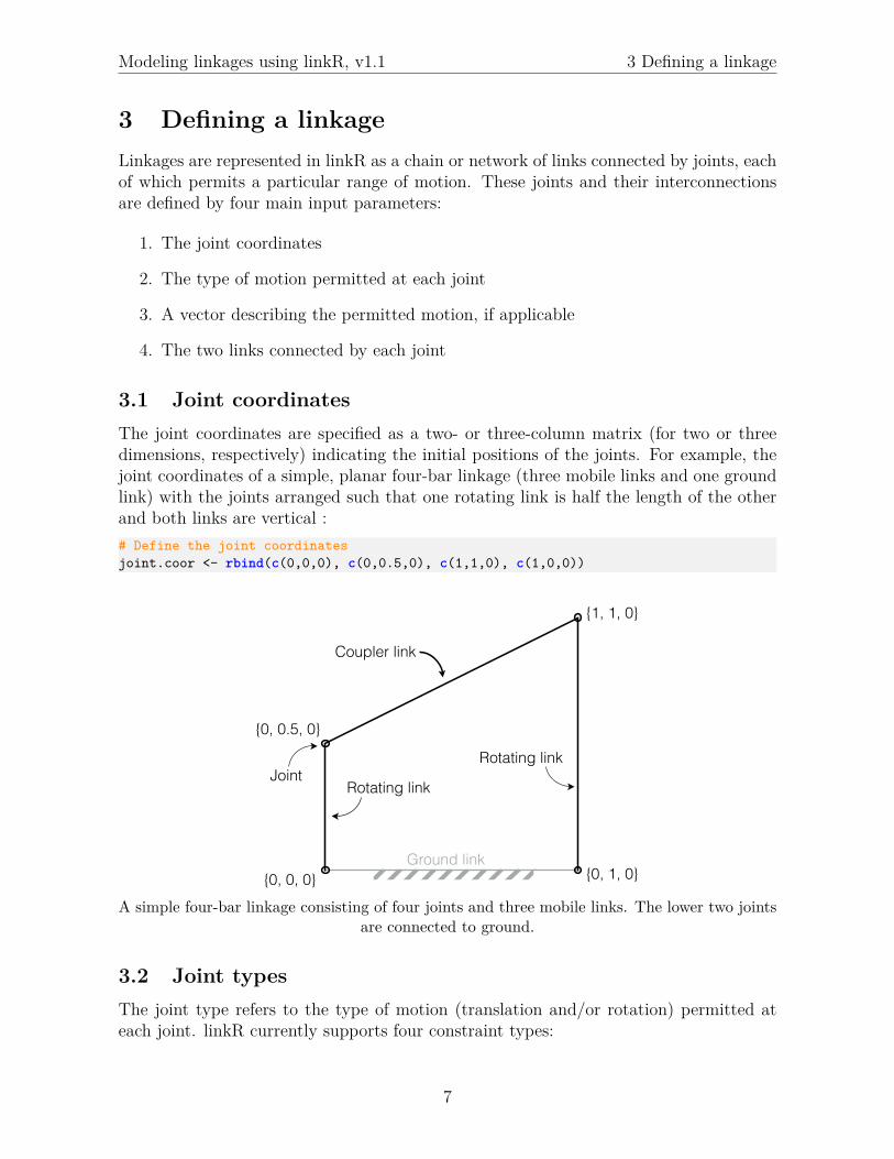
3.1 Joint coordinatesThe joint coordinates are specified as a two- or three-column matrix (for two or threedimensions, respectively) indicating the initial positions of the joints. For example, thejoint coordinates of a simple, planar four-bar linkage (three mobile links and one groundlink) with the joints arranged such that one rotating link is half the length of the otherand both links are vertical :# Define the joint coordinatesjoint.coor <- rbind(c(0,0,0), c(0,0.5,0), c(1,1,0), c(1,0,0))

{0, 0, 0}

{0, 0.5, 0}

{1, 1, 0}

{0, 1, 0}

JointRotating link

Ground link

Rotating link

Coupler link

A simple four-bar linkage consisting of four joints and three mobile links. The lower two jointsare connected to ground.

3.2 Joint typesThe joint type refers to the type of motion (translation and/or rotation) permitted ateach joint. linkR currently supports four constraint types:

7

Modeling linkages using linkR, v1.1 3.3 Joint constraint vectors

• Linear (L). Permits translation along a single line or vector

• Planar (P). Permits translation within a plane

• Rotational (R). Permits rotation about a single axis

• Spherical (S). Permits rotation about all three axes (including long-axis rotation)

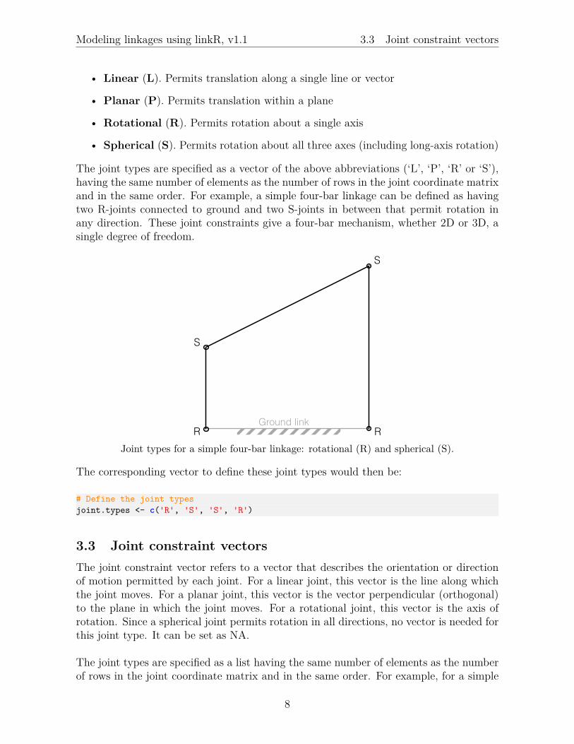
The joint types are specified as a vector of the above abbreviations (‘L’, ‘P’, ‘R’ or ‘S’),having the same number of elements as the number of rows in the joint coordinate matrixand in the same order. For example, a simple four-bar linkage can be defined as havingtwo R-joints connected to ground and two S-joints in between that permit rotation inany direction. These joint constraints give a four-bar mechanism, whether 2D or 3D, asingle degree of freedom.

R

S

S

RGround link

Joint types for a simple four-bar linkage: rotational (R) and spherical (S).

The corresponding vector to define these joint types would then be:

# Define the joint typesjoint.types <- c('R', 'S', 'S', 'R')

3.3 Joint constraint vectorsThe joint constraint vector refers to a vector that describes the orientation or directionof motion permitted by each joint. For a linear joint, this vector is the line along whichthe joint moves. For a planar joint, this vector is the vector perpendicular (orthogonal)to the plane in which the joint moves. For a rotational joint, this vector is the axis ofrotation. Since a spherical joint permits rotation in all directions, no vector is needed forthis joint type. It can be set as NA.

The joint types are specified as a list having the same number of elements as the numberof rows in the joint coordinate matrix and in the same order. For example, for a simple

8

Modeling linkages using linkR, v1.1 3.4 Joint connections

two-dimensional (planar) four-bar linkage, the axes of rotation at the two R-joints areoriented perpendicular to the plane of the linkage. For the previously given coordinatesthese vectors are oriented parallel to the z-axis.

# Define the joint constraint vectorsjoint.cons <- list(c(0,0,1), NA, NA, c(0,0,1))

R

S

S

RR

S

S

R

A B

The joint constraint vectors (blue) for two R-joints in a planar four-bar linkage seen in front(A) and oblique side view (B). The vectors are oriented orthogonal to the linkage plane.

3.4 Joint connectionsLinkages are defined in linkR as links interconnected by joints, with each joint connectingtwo links. The two links connected by each joint are specified in a two-column matrix inwhich each column corresponds to the two links and each row corresponds to each joint.Thus, the matrix should have the same number of rows, and be in the same order, as thejoint coordinate matrix.

Each linkage will have a single ground link, which is link 0. The numbering of theremaining links is arbitrary but will be used to associate linkage input motions with theappropriate link. For the simple four-bar linkage, the joint connects form a simple chain:the first joint connects the ground link to link 1, the second joint connects link 1 to link2, etc. The matrix defining the joint connections would be as follows:

# Define the connections among jointsjoint.conn <- rbind(c(0,1), c(1,2), c(2,3), c(3,0))

While each joint is allowed to connect only two links, links may be connected by anynumber of joints. For linkages that have parallel, interconnected sets of links this matrixthe ‘joint.conn’ matrix specifies these branched interconnections among the links.

9

Modeling linkages using linkR, v1.1 3.5 Calling ‘defineLinkage’

3.5 Calling ‘defineLinkage’These four inputs are passed to the function ‘defineLinkage’ in order to define the linkagefor kinematic simulation:

# Create a 'linkage' objectlinkage <- defineLinkage(joint.coor=joint.coor, joint.types=joint.types, joint.cons=

joint.cons, joint.conn=joint.conn)

The returned object (here, ‘linkage’) can be passed to other linkR functions for visualiza-tion and kinematic simulation. The linkR package uses a new R package, svgViewR, tocreate interactive, 3D animated visualizations of linkages that can be viewed in any majorweb browser. To visualize the linkage in its initial state, use ‘drawLinkage’, specifyingthe name of the file to be written to the current working directory.

# Create a linkage visualizationdrawLinkage(linkage, file='Linkage')

This will create an ‘html’ animation file using the specified file name.

Interactive linkage visualization in a web browser created by drawLinkage.

Once you open this file in a web browser, you can use the mouse to interact with thevisualization. In the top right corner of the browser window, click the icon (or holddown ‘r’) and then click and drag with the mouse to rotate the visualization. Click the

icon to turn on translation and click and drag to move the visualization around thewindow. Use scroll to zoom in and out. The viewing file is entirely self-contained so itcan be moved and viewed on any platform.

You can also visualize the linkage using the native R plot tools by calling drawLinkagewithout an input for ‘file’. However, this doesn’t provide the animation or interactivefeatures of the svgViewR visualization.

10


Modeling linkages using linkR, v1.1 3.6 Adding associated points

# Plot the linkage using native R plot device (static only)drawLinkage(linkage)

The four-bar linkage visualized in the R plot device.

3.6 Adding associated pointsSometimes you’ll want to simulate and track the motion of points on or associated with alink rather than the joints or links themselves. First define the coordinates of the points.The points defined below correspond the midpoint of each link.

# Define the point coordinateslink.points <- rbind(c(0,0.25,0), c(0.5,0.75,0), c(1,0.5,0))

Then specify the links with which each point is associated (in the same order as ‘link.points’).

# Set the link associations for each pointlink.assoc <- c(1,2,3)

Define the linkage, this time adding the input parameters ‘link.points’ and ‘link.assoc’.

# Define a linkage with associated pointslinkage <- defineLinkage(joint.coor=joint.coor, joint.types=joint.types, joint.cons=

joint.cons, joint.conn=joint.conn, link.points=link.points, link.assoc=link.assoc)

11

Modeling linkages using linkR, v1.1 3.7 Connecting associated points into shapes

4-bar with points associated with each link.

When you simulate motion of the linkage, the points will move with their correspondinglink allowing you to track motion at point in the linkage.

3.7 Connecting associated points into shapesIf you add points not located on the straight-line distance between joints it is easier tovisualize how these points are moving relative to one another (and relative to the links) byconnecting them with a path. For example, we could use four points to define rectanglesaround the two rotating links.

# Define first rectanglerec1 <- rbind(c(-0.1,-0.1,0), c(-0.1,0.6,0), c(0.1,0.6,0), c(0.1,-0.1,0))

# Define second rectanglerec2<- rbind(c(0.9,-0.1,0), c(0.9,1.1,0), c(1.1,1.1,0), c(1.1,-0.1,0))

# Define the point coordinateslink.points <- rbind(rec1, c(0.5,0.75,0), rec2)

# Set the link associations for each pointlink.assoc <- c(1,1,1,1, 2, 3,3,3,3)

12

Modeling linkages using linkR, v1.1 3.7 Connecting associated points into shapes

Specify the points you wish to connect in sequence to draw each path. Specify each pathas a separate element of a list.

# Define points to connect into pathspath.connect <- list(c(1:4,1), c(6:9,6))

Then define the linkage, adding the ‘path.connect’ parameter.

# Define the linkagelinkage <- defineLinkage(joint.coor=joint.coor, joint.types=joint.types, joint.cons=

joint.cons, joint.conn=joint.conn, link.points=link.points, link.assoc=link.assoc,path.connect=path.connect)

4-bar with points connected into rectangles around rotating links.

13

Modeling linkages using linkR, v1.1 4 Simulating linkage motion

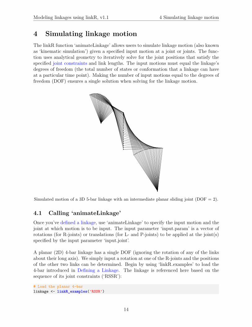
4 Simulating linkage motionThe linkR function ‘animateLinkage’ allows users to simulate linkage motion (also knownas ‘kinematic simulation’) given a specified input motion at a joint or joints. The func-tion uses analytical geometry to iteratively solve for the joint positions that satisfy thespecified joint constraints and link lengths. The input motions must equal the linkage’sdegrees of freedom (the total number of states or conformation that a linkage can haveat a particular time point). Making the number of input motions equal to the degrees offreedom (DOF) ensures a single solution when solving for the linkage motion.

Simulated motion of a 3D 5-bar linkage with an intermediate planar sliding joint (DOF = 2).

4.1 Calling ‘animateLinkage’Once you’ve defined a linkage, use ‘animateLinkage’ to specify the input motion and thejoint at which motion is to be input. The input parameter ‘input.param’ is a vector ofrotations (for R-joints) or translations (for L- and P-joints) to be applied at the joint(s)specified by the input parameter ‘input.joint’.

A planar (2D) 4-bar linkage has a single DOF (ignoring the rotation of any of the linksabout their long axis). We simply input a rotation at one of the R-joints and the positionsof the other two links can be determined. Begin by using ‘linkR examples’ to load the4-bar introduced in Defining a Linkage. The linkage is referenced here based on thesequence of its joint constraints (‘RSSR’):

# Load the planar 4-barlinkage <- linkR_examples('RSSR')

14

Modeling linkages using linkR, v1.1 4.1 Calling ‘animateLinkage’

Then use ‘animateLinkage’, rotating the first link over three angles from 0 to π4 radians

(0 to 45 degrees):

# Simulate with input rotations of 0, 22.5, and 45 deg at first R-jointanimate <- animateLinkage(linkage, input.param=c(0,pi/8,pi/4), input.joint=1)

Visualize this motion using ‘drawLinkage’:

# Create animated visualizationdrawLinkage(animate, file='Animate')

The drawLinkage function creates an interactive animation file using the R packagesvgViewR that can be opened in any major web browser. You can also create a staticvisualization, superimposing each frame, by setting the ‘animate’ parameter to FALSE:

# Create static visualizationdrawLinkage(animate, file='Static', animate=FALSE)

A 4-bar linkage with the first rotating link (left) rotated to 0, 22.5 and 45 degrees (all framessuperimposed).

Note that the input rotations follow the right-hand rule. Since the joint constraint vectoris positive along the z-axis, a positive angular rotation will rotate the link in a counter-clockwise direction when viewed such that the positive z-axis is pointing toward theviewer (as above).

To specify the input rotations at the other rotating link, change ‘input.joint’ to ‘4’ sincethe second R-joint was the fourth joint when defining the joint types.

# Simulate with input rotations of 0, 22.5, and 45 deg at second R-jointanimate <- animateLinkage(linkage, input.param=c(0,pi/8,pi/4), input.joint=4)

# Create animationdrawLinkage(animate, file='Animate_4')

15



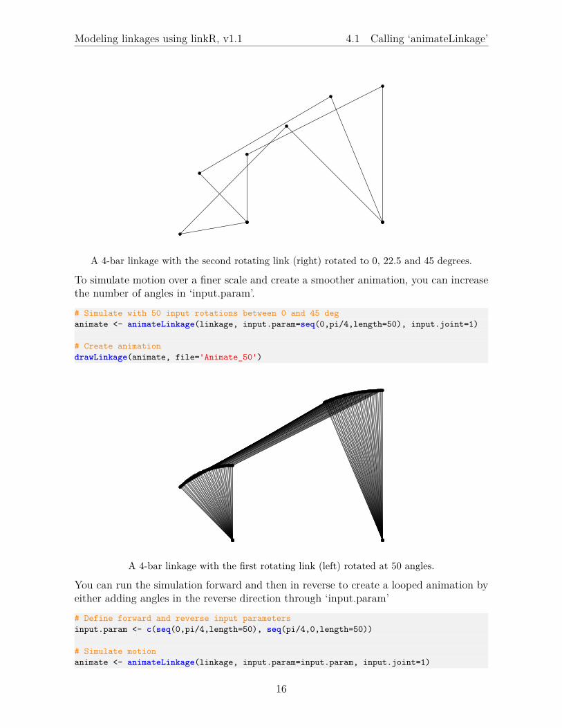
A 4-bar linkage with the second rotating link (right) rotated to 0, 22.5 and 45 degrees.

To simulate motion over a finer scale and create a smoother animation, you can increasethe number of angles in ‘input.param’.# Simulate with 50 input rotations between 0 and 45 deganimate <- animateLinkage(linkage, input.param=seq(0,pi/4,length=50), input.joint=1)

# Create animationdrawLinkage(animate, file='Animate_50')

A 4-bar linkage with the first rotating link (left) rotated at 50 angles.

You can run the simulation forward and then in reverse to create a looped animation byeither adding angles in the reverse direction through ‘input.param’# Define forward and reverse input parametersinput.param <- c(seq(0,pi/4,length=50), seq(pi/4,0,length=50))

# Simulate motionanimate <- animateLinkage(linkage, input.param=input.param, input.joint=1)

16


or by setting the ‘animate.reverse’ argument for drawLinkage to TRUE.

# Simulate with 50 input rotations between 0 and 45 deganimate <- animateLinkage(linkage, input.param=seq(0,pi/4,length=50), input.joint=1)

# Create animation with forward-reverse loopdrawLinkage(animate, file='Animate_loop', animate.reverse=TRUE)

Note that if you’re performing analysis on the simulated motion, creating a loop using‘animate.reverse’ will only affect the visualization file, not the simulation results them-selves.

17

Modeling linkages using linkR, v1.1 5 Analyzing linkage motion

5 Analyzing linkage motionOnce you’ve simulated linkage motion over a range of conformations you can track therelative motion of the links or different points within the linkage to quantify relative mo-tion of linkage elements, calculate transmission metrics (e.g. mechanical advantage), orperform further analyses. The function ‘linkageKinematics’ takes as input the simulatedmotion of a linkage and pulls out the motion of the joints, links, and associated points,which can then be used in subsequent analyses.

5.1 Joint position over timeTo demonstrate a few approaches to linkage analysis we’ll take the previously introduced4-bar linkage and rotate the smaller link a full 360 degrees.

# Load the tutorial 4-bar linkage with associated pointslinkage <- linkR_examples('RSSR_points')

# Input a 360 deg (2*pi rad) rotation of the shorter linkanimate <- animateLinkage(linkage, input.param=seq(0,2*pi,length=60), input.joint=1)

# Create animation with forward-reverse loopdrawLinkage(animate, file='Analyze')

A 4-bar linkage with the shorter link rotated 360 deg (all frames superimposed). Associatedpoints are omitted for clarity.

Note that because of the linkage configuration a full rotation of the smaller link onlyresults in a partial rotation of the larger link.

18

Modeling linkages using linkR, v1.1 5.1 Joint position over time

To obtain the coordinates of all the joints in the linkage over the simulated iterations,access the ‘joint.coor’ object of the list returned by ‘animateLinkage’ (here, ‘animate’).

# Array of joint coordinates over iterationsjoints <- animate$joint.coor

‘joint.coor’ is a 3D array in which the first dimension corresponds to the joints, the secondcorresponds to the xyz-coordinates, and the third corresponds to the animation frame.For example, the following code plots the xy-coordinates of the second joint (the jointbetween the short rotating link and the coupler link) through the simulation. Since thisis a planar linkage, the z-coordinate doesn’t change and the z-vs-t plot can be replacedwith a y-vs-x plot.

# Open 3-column, multipanel plot with specified marginspar(mfrow=c(1,3), mar=c(4,4,0.5,0.5))

# Plot xy-coordinates joint over iterationsfor(i in 1:2) plot(joints[2, i, ], type='l', ylab=c('x','y')[i], xlab='i')

# Plot xy-coordinates in y-vs-x plotplot(x=joints[2,1,], y=joints[2,2,], type='l', xlab='x', ylab='y')

0 10 20 30 40 50 60

−0.

4−

0.2

0.0

0.2

0.4

i

x

0 10 20 30 40 50 60

−0.

4−

0.2

0.0

0.2

0.4

i

y

−0.4 −0.2 0.0 0.2 0.4

−0.

4−

0.2

0.0

0.2

0.4

x

y

The change in the xy-coordinates of the second joint in an animated 4-bar linkage.

Since this joint is attached to a rotating link that makes a full rotation, its motiondescribes a circle. The motion of the longer link is more complex, rotating at a non-constant rate over a partial arc. This can be seen by plotting the third joint in thelinkage (the joint between the coupler link and the second rotating link).


# Plot xy-coordinates joint over iterationsfor(i in 1:2) plot(joints[3, i, ], type='l', ylab=c('x','y')[i], xlab='i')

# Plot xy-coordinates in y-vs-x plotplot(x=joints[3,1,], y=joints[3,2,], type='l', xlab='x', ylab='y')

19

Modeling linkages using linkR, v1.1 5.2 Point position over time

0 10 20 30 40 50 60

0.2

0.4

0.6

0.8

1.0

1.2

i

x

0 10 20 30 40 50 60

0.6

0.7

0.8

0.9

1.0

i

y

0.2 0.4 0.6 0.8 1.0 1.2

0.6

0.7

0.8

0.9

1.0

x

y

The change in the xy-coordinates of the third joint in an animated 4-bar linkage.

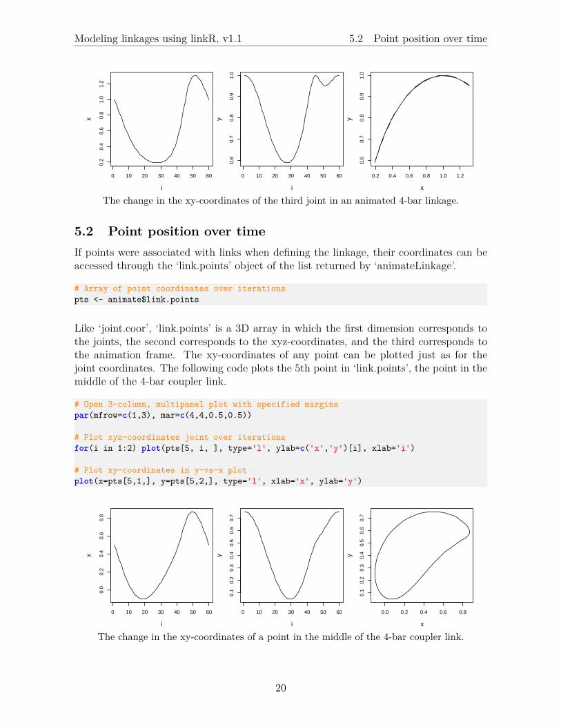
5.2 Point position over timeIf points were associated with links when defining the linkage, their coordinates can beaccessed through the ‘link.points’ object of the list returned by ‘animateLinkage’.

# Array of point coordinates over iterationspts <- animate$link.points

Like ‘joint.coor’, ‘link.points’ is a 3D array in which the first dimension corresponds tothe joints, the second corresponds to the xyz-coordinates, and the third corresponds tothe animation frame. The xy-coordinates of any point can be plotted just as for thejoint coordinates. The following code plots the 5th point in ‘link.points’, the point in themiddle of the 4-bar coupler link.


# Plot xyz-coordinates joint over iterationsfor(i in 1:2) plot(pts[5, i, ], type='l', ylab=c('x','y')[i], xlab='i')

# Plot xy-coordinates in y-vs-x plotplot(x=pts[5,1,], y=pts[5,2,], type='l', xlab='x', ylab='y')

0 10 20 30 40 50 60

0.0

0.2

0.4

0.6

0.8

i

x

0 10 20 30 40 50 60

0.1

0.2

0.3

0.4

0.5

0.6

0.7

i

y

0.0 0.2 0.4 0.6 0.8

0.1

0.2

0.3

0.4

0.5

0.6

0.7

x

y

The change in the xy-coordinates of a point in the middle of the 4-bar coupler link.

20

Modeling linkages using linkR, v1.1 5.3 Calling ‘linkageKinematics’

5.3 Calling ‘linkageKinematics’For certain analyses we might be interested not just in the positions of the joints andassociated points but also in their velocity (i.e. derivatives of their position over theanimation). Also, we might be interested in the angular displacements (i.e. rotation) ofthe links and its derivative, angular velocity. The ‘linkageKinematics’ function calculatesthese quantities to streamline kinematic analysis.

# Measure linkage kinematicskine <- linkageKinematics(animate)

The function returns the kinematics of joint translation, link rotation, and associatedpoint translation. For joints and points these kinematic results are accessed by appendingthe following to ‘joints’ or ‘points’ (e.g. ‘joints.t’, ‘points.tdis.d’):

1. t: Displacement of each joint/point in each dimension (3D array)

2. tdis: Total displacement of each joint/point (2D matrix)

3. t.d: Velocity of each joint/point in each dimension (the derivative of 1, 3D array)

4. tdis.d: Total velocity of each joint/point (the derivative of 2, 2D matrix)

The kinematic results for links are similar except that they measure rotation rather thantranslation (replacing ‘t’ with ‘r’). These can be accessed by appending the following to‘links’ (e.g. ‘links.r’, links.rdis.d’):

1. r: Angular displacement of each link about each axis (3D array)

2. rdis: Total angular displacement of each link (2D matrix)

3. r.d: Angular velocity of each link about each axis (the derivative of 1, 3D array)

4. rdis.d: Total angular velocity of each link (the derivative of 2, 2D matrix)

In the context of rotation, “angular displacements about each axis” refers to the magni-tudes of a series of rotations about the z, y, and x-axes, in that order, that reproducesthe full rotation, so called ‘Euler angles’. Note that because links can move with bothtranslational and rotational components, different points on a single link can displace todiffering extents. Thus, for whole link motion only rotation is quantified while joints andlink-associated points provide a means to track translational motion at any point in alinkage.

Displacements are measured relative to the first iteration. Also, the “derivatives” arecalculated simply by taking the difference between consecutive iterations. For this reason,the first iteration will always be NA. The smoothness or resolution of the derivatives willdepend on the motion between consecutive iterations. To increase the smoothness simplyincrease the number of iterations. The derivatives are calculated with respect to iterationsor steps, rather than time.

21

Modeling linkages using linkR, v1.1 5.4 Angular displacement and velocity of links

5.4 Angular displacement and velocity of linksTo access the Euler components of link angular displacement and velocity, use the objects‘links.r’ and ‘linkr.r.d’, respectively. For example, the following code plots the angulardisplacement and velocity of the longer rotating link in the 4-bar linkage about the z-axis. If no link names are provided, link names are automatically assigned as ‘Ground’,‘Link1’, ‘Link2’, etc. The longer rotating link in the previously introduced 4-bar linkageis the third link or ‘Link3’.


# Plot z-axis angular displacement, velocity, and displacement vs. velocityplot(kine$links.r['Link3',3,], type='l', xlab='i', ylab='Ang. disp. along z')plot(kine$links.r.d['Link3',3,], type='l', xlab='i', ylab='Ang. vel. along z')plot(x=kine$links.r['Link3',3,], y=kine$links.r.d['Link3',3,], type='l',

xlab='Ang. disp. along z', ylab='Ang. vel. along z')

0 10 20 30 40 50 60

−0.

20.

00.

20.

40.

60.

8

i

Ang

. dis

p. a

long

z

0 10 20 30 40 50 60

−0.

10−

0.05

0.00

0.05

i

Ang

. vel

. alo

ng z

−0.2 0.0 0.2 0.4 0.6 0.8

−0.

10−

0.05

0.00

0.05

Ang. disp. along z

Ang

. vel

. alo

ng z

Angular displacement and velocity of the longer rotating link (z-axis component) in the 4-barlinkage.

To access the total angular displacements and velocities of links (i.e. not the rotationalcomponents), use the objects ‘links.rdis’ and ‘links.rdis.d’, respectively. For example, thefollowing code plots the total angular displacement and velocity of the longer rotatinglink in the 4-bar linkage.


# Plot total angular displacement, velocity, and displacement vs. velocityplot(kine$links.rdis['Link3',],type='l',xlab='i',ylab='Ang. disp. along z')plot(kine$links.rdis.d['Link3',],type='l',xlab='i',ylab='Ang. vel. along z')plot(x=kine$links.rdis['Link3',], y=kine$links.rdis.d['Link3',], type='l',

xlab='Ang. disp. along z', ylab='Ang. vel. along z')

Except for the sign of the angular displacements, the total angular displacements are thesame as the rotational components along the z-axis. This is because the link is constrainedto rotate entirely about the z-axis and therefore has no rotational component about thex- and y-axes.

22

Modeling linkages using linkR, v1.1 5.5 Displacement and velocity of joints

0 10 20 30 40 50 60

−0.

8−

0.4

0.0

0.2

i

Ang

. dis

p. a

long

z

0 10 20 30 40 50 60

−0.

050.

000.

050.

10

i

Ang

. vel

. alo

ng z

−0.8 −0.6 −0.4 −0.2 0.0 0.2

−0.

050.

000.

050.

10

Ang. disp. along z

Ang

. vel

. alo

ng z

Total angular displacement and velocity of the longer rotating link in the 4-bar linkage.

5.5 Displacement and velocity of jointsTo access the displacements and velocities of joints along a particular dimension, use theobjects ‘joints.t’ and ‘joints.t.d’, respectively. For example, the following code plots thex-axis displacement and velocity of the third joint in the 4-bar linkage.


# Plot x-axis displacement, velocity, and displacement vs. velocityplot(kine$joints.t[3,1,], type='l', xlab='i', ylab='Displacement along x')plot(kine$joints.t.d[3,1,], type='l', xlab='i', ylab='Velocity along x')plot(x=kine$joints.t[3,1,], y=kine$joints.t.d[3,1,], type='l',

xlab='Displacement along x', ylab='Velocity along x')

0 10 20 30 40 50 60

−0.

8−

0.6

−0.

4−

0.2

0.0

0.2

i

Dis

plac

emen

t alo

ng x

0 10 20 30 40 50 60

−0.

050.

000.

050.

10

i

Vel

ocity

alo

ng x

−0.8 −0.6 −0.4 −0.2 0.0 0.2

−0.

050.

000.

050.

10

Displacement along x

Vel

ocity

alo

ng x

Displacement and velocity along the x-axis of the third joint in the 4-bar linkage.

The displacement plots of the third joint look very similar to the angular displacementplots of the longer rotating link because the joint rotates with the link at a distance ofexactly 1 from the points of rotation.

To access the total displacements and velocities of joints, use the objects ‘joints.tdis’ and‘joints.tdis.d’, respectively. For example, the following code plots the total displacementand velocity of the third joint in the 4-bar linkage.

23

Modeling linkages using linkR, v1.1 5.6 Displacement and velocity of points


# Plot total displacement, velocity, and displacement vs. velocityplot(kine$joints.tdis[3,], type='l', xlab='i', ylab='Displacement')plot(kine$joints.tdis.d[3,], type='l', xlab='i', ylab='Velocity')plot(x=kine$joints.tdis[3,], y=kine$joints.tdis.d[3,], type='l',

xlab='Displacement', ylab='Velocity')

0 10 20 30 40 50 60

0.0

0.2

0.4

0.6

0.8

i

Dis

plac

emen

t

0 10 20 30 40 50 60

0.00

0.02

0.04

0.06

0.08

0.10

i

Vel

ocity

0.0 0.2 0.4 0.6 0.8

0.00

0.02

0.04

0.06

0.08

0.10

Displacement

Vel

ocity

Total displacement and velocity along the x-axis of the second joint in the 4-bar linkage.

Note that because these are total displacements from the initial position they can onlybe positive.

5.6 Displacement and velocity of pointsThe displacements and velocities of points associated with links can be accessed inthe same manner as joints, simply replacing ‘joints’ with ‘points’ (i.e. ‘points.t’ and‘points.t.d’). For example, the following code plots the x-axis displacement and velocityof the point attached to the middle of the 4-bar coupler link.# Open 3-column, multipanel plot with specified marginspar(mfrow=c(1,3), mar=c(4,4,0.5,0.5))

# Plot x-axis displacement, velocity, and displacement vs. velocityplot(kine$points.t[5,1,], type='l', xlab='i', ylab='Displacement along x')plot(kine$points.t.d[5,1,], type='l', xlab='i', ylab='Velocity along x')plot(x=kine$points.t[5,1,], y=kine$points.t.d[5,1,], type='l',

xlab='Displacement along x', ylab='Velocity along x')

0 10 20 30 40 50 60

−0.

6−

0.4

−0.

20.

00.

20.

4

i

Dis

plac

emen

t alo

ng x

0 10 20 30 40 50 60

−0.

040.

000.

020.

040.

06

i

Vel

ocity

alo

ng x

−0.6 −0.4 −0.2 0.0 0.2 0.4

−0.

040.

000.

020.

040.

06

Displacement along x

Vel

ocity

alo

ng x

24

Modeling linkages using linkR, v1.1 5.7 Torque mechanical advantage

Displacement and velocity along the x-axis of the point in the middle of the 4-bar coupler link.

To access the total displacements and velocities of points, use the objects ‘points.tdis’ and‘points.tdis.d’, respectively. For example, the following code plots the total displacementand velocity of the point in the middle of the 4-bar coupler link.


# Plot total displacement, velocity, and displacement vs. velocityplot(kine$points.tdis[5,], type='l', xlab='i', ylab='Displacement')plot(kine$points.tdis.d[5,], type='l', xlab='i', ylab='Velocity')plot(x=kine$points.tdis[5,], y=kine$points.tdis.d[5,], type='l',

xlab='Displacement', ylab='Velocity')

0 10 20 30 40 50 60

0.0

0.2

0.4

0.6

0.8

i

Dis

plac

emen

t

0 10 20 30 40 50 60

0.02

0.03

0.04

0.05

0.06

0.07

i

Vel

ocity

0.0 0.2 0.4 0.6 0.80.

020.

030.

040.

050.

060.

07

Displacement

Vel

ocity

Total displacement and velocity of the point in the middle of the 4-bar coupler link.

5.7 Torque mechanical advantageThe derivatives of displacement can be used to calculate metrics such as mechanical ad-vantage and kinematic transmission. These metrics measure the amplification of relativeforce (or torque) and velocity through a mechanism (for more details see Olsen and West-neat 2016).

For rotating links, the derivative of angular displacement can be used to calculate torquemechanical advantage (tMA). Torque MA is equal to the angular velocity of an input linkdivided by the angular velocity of an output link (the time derivatives of these velocitiesare absent because they cancel out when taking the ratio). Torque MA is also equal tothe ratio of output link torque divided by the input link torque.

tMA = dθidθo

= dτodτi

(1)

A linkage with a torque MA greater than 1 transforms an input torque into a relativelylarger output torque. This occurs at the expense of displacement - the output link alsorotates over a relatively smaller angle than the input link. Another metric common in

25

http://doi.org/10.1002/jmor.20596


Modeling linkages using linkR, v1.1 5.7 Torque mechanical advantage

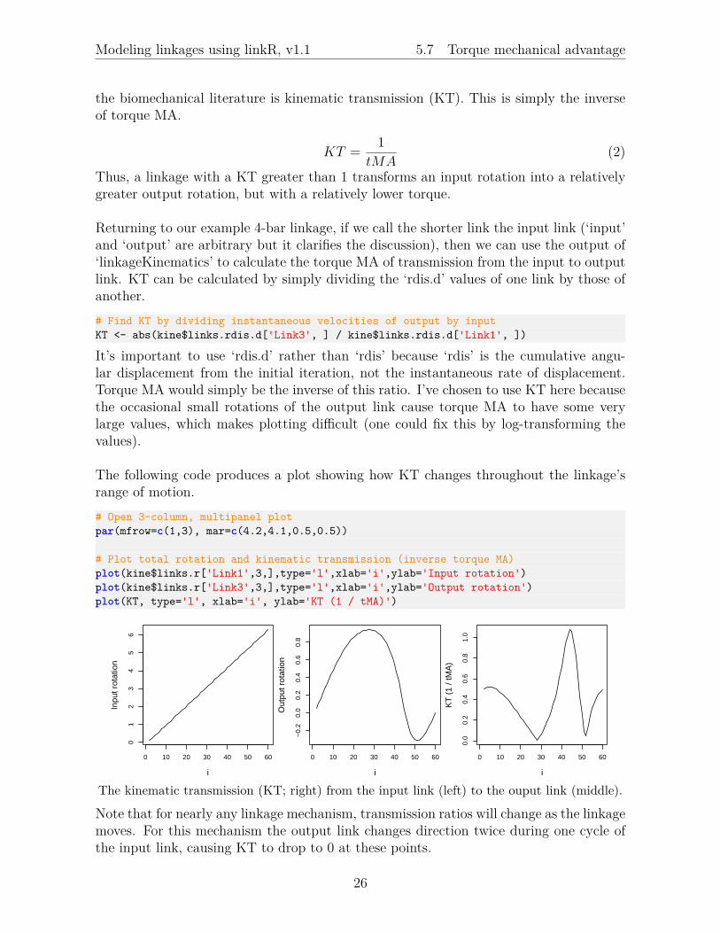
the biomechanical literature is kinematic transmission (KT). This is simply the inverseof torque MA.

KT = 1tMA

(2)

Thus, a linkage with a KT greater than 1 transforms an input rotation into a relativelygreater output rotation, but with a relatively lower torque.

Returning to our example 4-bar linkage, if we call the shorter link the input link (‘input’and ‘output’ are arbitrary but it clarifies the discussion), then we can use the output of‘linkageKinematics’ to calculate the torque MA of transmission from the input to outputlink. KT can be calculated by simply dividing the ‘rdis.d’ values of one link by those ofanother.# Find KT by dividing instantaneous velocities of output by inputKT <- abs(kine$links.rdis.d['Link3', ] / kine$links.rdis.d['Link1', ])

It’s important to use ‘rdis.d’ rather than ‘rdis’ because ‘rdis’ is the cumulative angu-lar displacement from the initial iteration, not the instantaneous rate of displacement.Torque MA would simply be the inverse of this ratio. I’ve chosen to use KT here becausethe occasional small rotations of the output link cause torque MA to have some verylarge values, which makes plotting difficult (one could fix this by log-transforming thevalues).

The following code produces a plot showing how KT changes throughout the linkage’srange of motion.# Open 3-column, multipanel plotpar(mfrow=c(1,3), mar=c(4.2,4.1,0.5,0.5))

# Plot total rotation and kinematic transmission (inverse torque MA)plot(kine$links.r['Link1',3,],type='l',xlab='i',ylab='Input rotation')plot(kine$links.r['Link3',3,],type='l',xlab='i',ylab='Output rotation')plot(KT, type='l', xlab='i', ylab='KT (1 / tMA)')

0 10 20 30 40 50 60

01

23

45

6

i

Inpu

t rot

atio

n

0 10 20 30 40 50 60

−0.

20.

00.

20.

40.

60.

8

i

Out

put r

otat

ion

0 10 20 30 40 50 60

0.0

0.2

0.4

0.6

0.8

1.0

i

KT

(1

/ tM

A)

The kinematic transmission (KT; right) from the input link (left) to the ouput link (middle).

Note that for nearly any linkage mechanism, transmission ratios will change as the linkagemoves. For this mechanism the output link changes direction twice during one cycle ofthe input link, causing KT to drop to 0 at these points.

26

Modeling linkages using linkR, v1.1 5.8 Force mechanical advantage

5.8 Force mechanical advantageTorque MA is only valid for rotating links and gives information related to angular ve-locity and torques. For mechanisms with links that move with some combination oftranslation and rotation or if you have some predetermined points at which forces areinput and output, it is better to use force mechanical advantage (fMA). Force MA isessentially the linear (non-rotational) analogue to torque MA, representing the amplifi-cation of output force (relative to input force). Thus, force MA is equal to the ratio ofthe linear velocities or the ratio of output force to input force.

fMA = dxidxo

= FoFi

(3)

Analogous to KT, force MA can be calculated by simply dividing the ‘tdis.d’ values ofone point in the linkage by those of another. The following code uses the joint betweenthe input link and coupler link as the point of input force and the point in the middle ofthe coupler link as the point of output force.

# Find fMA by dividing instantaneous linear velocities of input by outputfMA <- abs(kine$joints.tdis.d[2, ] / kine$points.tdis.d[5, ])

The fMA can then be plotted along with the input and output displacements. The inverseof force MA is plotted below because occasional translations of the coupler link causeforce MA to have some very large values.

# Open 3-column, multipanel plotpar(mfrow=c(1,3), mar=c(4.2,4.1,0.5,0.5))

# Plot total rotation and kinematic transmission (inverse torque MA)plot(kine$joints.tdis[2,],type='l',xlab='i',ylab='Input displacement')plot(kine$points.tdis[5,],type='l',xlab='i',ylab='Output displacement')plot(1/fMA, type='l', xlab='i', ylab='1 / fMA')

0 10 20 30 40 50 60

0.0

0.2

0.4

0.6

0.8

1.0

i

Inpu

t dis

plac

emen

t

0 10 20 30 40 50 60

0.0

0.2

0.4

0.6

0.8

i

Out

put d

ispl

acem

ent

0 10 20 30 40 50 60

0.4

0.6

0.8

1.0

1.2

1.4

i

1 / f

MA

The inverse force MA (right) of transmission from the joint between the input link andcoupler link (left) to the point in the middle of the coupler link (middle).

27

Modeling linkages using linkR, v1.1 6 Examples

6 Examples

6.1 Planar 4-bar (RSSR)

Planar 4-bar linkage (DOF=1). Three iterations shown.

# Define the joint coordinatesjoint.coor <- rbind(c(0,0,0), c(0,0.5,0), c(1,1,0), c(1,0,0))




# Define first rectanglerec1 <- rbind(c(-0.1,-0.1,0), c(-0.1,0.6,0), c(0.1,0.6,0), c(0.1,-0.1,0))





28

Modeling linkages using linkR, v1.1 6.2 3D 4-bar (RSSR)

# Define linkagelinkage <- defineLinkage(joint.coor=joint.coor, joint.types=joint.types,

joint.cons=joint.cons, joint.conn=joint.conn, link.points=link.points,link.assoc=link.assoc, path.connect=path.connect)

# Animate linkageanim <- animateLinkage(linkage, input.param=seq(0,2*pi,length=60), input.joint=1)

# Draw linkagedrawLinkage(anim, file='RSSR.html')

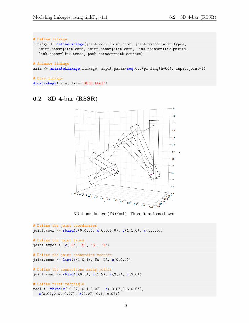
6.2 3D 4-bar (RSSR)

3D 4-bar linkage (DOF=1). Three iterations shown.

# Define the joint coordinatesjoint.coor <- rbind(c(0,0,0), c(0,0.5,0), c(1,1,0), c(1,0,0))




# Define first rectanglerec1 <- rbind(c(-0.07,-0.1,0.07), c(-0.07,0.6,0.07),

c(0.07,0.6,-0.07), c(0.07,-0.1,-0.07))

29

Modeling linkages using linkR, v1.1 6.3 Two coupled sliders (LSSL)







# Animate linkageanim <- animateLinkage(linkage, input.param=seq(0,2*pi,length=60), input.joint=1)

# Draw linkagedrawLinkage(anim, file='RSSR_3d.html')

6.3 Two coupled sliders (LSSL)

Linkage with two coupled linear sliding links (DOF=1). Three iterations shown.

# Define joint coordinatesjoint.coor <- rbind(c(0,0,0), c(0,0.1,0), c(0.9,0.5,0), c(1,0.5,0))

30

Modeling linkages using linkR, v1.1 6.4 Coupled planar and linear sliders (SSPSSL)

# Define joint typesjoint.types <- c("L", "S", "S", "L")

# Define joint constraintsjoint.cons <- list(c(1,0,0), NA, NA, c(0,1,0))

# Define points associated with linkslink.points <- rbind(c(-0.3,0,0), c(1,0,0), c(-0.1,0,0), c(-0.1,0.1,0), c(0.1,0.1,0),

c(0.1,0,0), c(1,0.4,0), c(0.9,0.4,0), c(0.9,0.6,0), c(1,0.6,0), c(1,0,0), c(1,1.2,0),

c(0.45, 0.3, 0))

# Define links with which points are associatedlink.assoc <- c(0,0,1,1,1,1,3,3,3,3,0,0,2)

# Define lines connecting associated pointspath.connect <- list(c(1,2), c(3:6,3), c(7:10,7), c(11,12))


joint.cons=joint.cons, link.points=link.points, link.assoc=link.assoc,path.connect=path.connect)

# Animate linkageanim <- animateLinkage(linkage, input.param=seq(0,0.5,length=50), input.joint=1)

# Draw linkagedrawLinkage(anim, file='LSSL.html', animate.reverse=TRUE)

6.4 Coupled planar and linear sliders (SSPSSL)

31

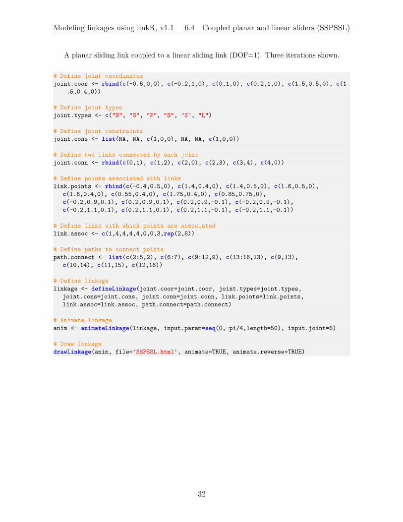
Modeling linkages using linkR, v1.1 6.4 Coupled planar and linear sliders (SSPSSL)

A planar sliding link coupled to a linear sliding link (DOF=1). Three iterations shown.

# Define joint coordinatesjoint.coor <- rbind(c(-0.6,0,0), c(-0.2,1,0), c(0,1,0), c(0.2,1,0), c(1.5,0.5,0), c(1

.5,0.4,0))

# Define joint typesjoint.types <- c("S", "S", "P", "S", "S", "L")

# Define joint constraintsjoint.cons <- list(NA, NA, c(1,0,0), NA, NA, c(1,0,0))

# Define two links connected by each jointjoint.conn <- rbind(c(0,1), c(1,2), c(2,0), c(2,3), c(3,4), c(4,0))

# Define points associated with linkslink.points <- rbind(c(-0.4,0.5,0), c(1.4,0.4,0), c(1.4,0.5,0), c(1.6,0.5,0),

c(1.6,0.4,0), c(0.55,0.4,0), c(1.75,0.4,0), c(0.85,0.75,0),c(-0.2,0.9,0.1), c(0.2,0.9,0.1), c(0.2,0.9,-0.1), c(-0.2,0.9,-0.1),c(-0.2,1.1,0.1), c(0.2,1.1,0.1), c(0.2,1.1,-0.1), c(-0.2,1.1,-0.1))

# Define links with which points are associatedlink.assoc <- c(1,4,4,4,4,0,0,3,rep(2,8))

# Define paths to connect pointspath.connect <- list(c(2:5,2), c(6:7), c(9:12,9), c(13:16,13), c(9,13),

c(10,14), c(11,15), c(12,16))



# Animate linkageanim <- animateLinkage(linkage, input.param=seq(0,-pi/4,length=50), input.joint=6)

# Draw linkagedrawLinkage(anim, file='SSPSSL.html', animate=TRUE, animate.reverse=TRUE)

32

Modeling linkages using linkR, v1.1 6.5 Three coupled sliders (LSSLSSL)

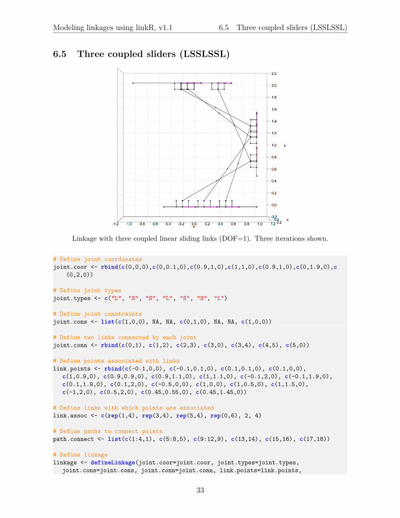
6.5 Three coupled sliders (LSSLSSL)

Linkage with three coupled linear sliding links (DOF=1). Three iterations shown.

# Define joint coordinatesjoint.coor <- rbind(c(0,0,0),c(0,0.1,0),c(0.9,1,0),c(1,1,0),c(0.9,1,0),c(0,1.9,0),c

(0,2,0))

# Define joint typesjoint.types <- c("L", "S", "S", "L", "S", "S", "L")

# Define joint constraintsjoint.cons <- list(c(1,0,0), NA, NA, c(0,1,0), NA, NA, c(1,0,0))

# Define two links connected by each jointjoint.conn <- rbind(c(0,1), c(1,2), c(2,3), c(3,0), c(3,4), c(4,5), c(5,0))

# Define points associated with linkslink.points <- rbind(c(-0.1,0,0), c(-0.1,0.1,0), c(0.1,0.1,0), c(0.1,0,0),

c(1,0.9,0), c(0.9,0.9,0), c(0.9,1.1,0), c(1,1.1,0), c(-0.1,2,0), c(-0.1,1.9,0),c(0.1,1.9,0), c(0.1,2,0), c(-0.5,0,0), c(1,0,0), c(1,0.5,0), c(1,1.5,0),c(-1,2,0), c(0.5,2,0), c(0.45,0.55,0), c(0.45,1.45,0))

# Define links with which points are associatedlink.assoc <- c(rep(1,4), rep(3,4), rep(5,4), rep(0,6), 2, 4)

# Define paths to connect pointspath.connect <- list(c(1:4,1), c(5:8,5), c(9:12,9), c(13,14), c(15,16), c(17,18))


joint.cons=joint.cons, joint.conn=joint.conn, link.points=link.points,

33

Modeling linkages using linkR, v1.1 6.6 Crank-driving sliding link (RSSL)

link.assoc=link.assoc, path.connect=path.connect)

# Animate linkageanim <- animateLinkage(linkage, input.param=seq(-0.2, 0.5, length=50), input.joint=1)

# Draw linkagedrawLinkage(anim, file='LSSLSSL.html', animate.reverse=TRUE)

6.6 Crank-driving sliding link (RSSL)

Rotating link coupled with sliding link (DOF=1). Three iterations shown.

# Define joint coordinatesjoint.coor <- rbind(c(0,0,0), c(0,1,0), c(0.9,0.6,0), c(1,0.5,0))

# Define joint typesjoint.types <- c("R", "S", "S", "L")

# Define joint constraintsjoint.cons <- list(c(1,0,1), NA, NA, c(1,1,0))

# Define two links connected by each jointjoint.conn <- rbind(c(0,1), c(1,2), c(2,3), c(3,0))

# Define points associated with linkslink.points <- rbind(c(0.75,0.25,0), c(1.75,1.25,0), c(0.9,0.4,0), c(0.8,0.5,0),

c(1,0.7,0), c(1.1,0.6,0), c(0.1,0,0.1), c(-0.1,0,-0.1), c(-0.05,0,0.05),c(-0.05,1,0.05), c(0.05,1,-0.05), c(0.05,0,-0.05), c(0.45,0.8,0))

# Define links with which points are associatedlink.assoc <- c(0,0,3,3,3,3,0,0,1,1,1,1,2)

34

Modeling linkages using linkR, v1.1 6.7 Slider along rotating link (RLSS)

# Define paths to connect pointspath.connect <- list(c(1,2), c(3:6,3), c(7,8), c(9:12,9))




# DRAW LINKAGEdrawLinkage(anim, file='RSSL.html', animate.reverse=TRUE)

6.7 Slider along rotating link (RLSS)

Link sliding along a rotating link (DOF=1). Three iterations shown.

# Define joint coordinatesjoint.coor <- rbind(c(0,0,0), c(0,0.75,0), c(0.1,0.75,0), c(0.8,0.4,0))

# Define joint typesjoint.types <- c("R", "L", "S", "S")

# Define joint constraintsjoint.cons <- list(c(0,0,1), c(0,1,0), NA, NA)

# Define link nameslink.names <- c('Ground', 'L1', 'L2', 'L3')

35

Modeling linkages using linkR, v1.1 6.8 Rotating links in series (RRSS)

# Define two links connected by each jointjoint.conn <- rbind(c('Ground','L1'), c('L1','L2'), c('L2','L3'), c('L3','Ground'))

# Define points associated with linkslink.points <- rbind(c(0,0.65,0), c(0.1,0.65,0), c(0.1,0.85,0), c(0,0.85,0),

c(0,0,0), c(-0.1,0,0), c(-0.1,1.5,0), c(0,1.5,0), c(0.45, 0.575, 0))

# Define links with which points are associatedlink.assoc <- c(2,2,2,2,1,1,1,1,3)

# Define lines connecting associated pointspath.connect <- list(c(1:4,1), c(5:8,5))


joint.cons=joint.cons, joint.conn=joint.conn, link.names=link.names,link.points=link.points, link.assoc=link.assoc, path.connect=path.connect)

# Animate linkageanim <- animateLinkage(linkage, input.param=seq(0,-0.4,length=50), input.joint=1)

# Draw linkagedrawLinkage(anim, file='RLSS.html', animate.reverse=TRUE)

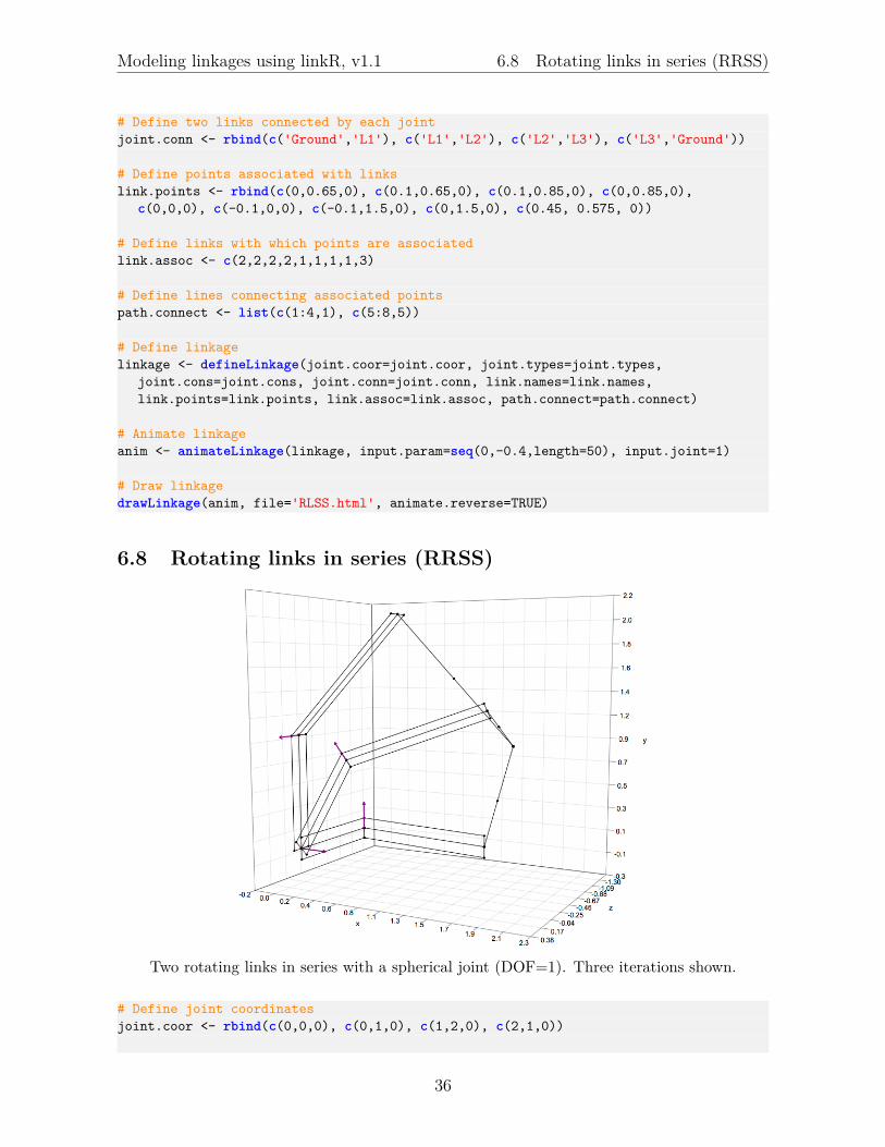
6.8 Rotating links in series (RRSS)

Two rotating links in series with a spherical joint (DOF=1). Three iterations shown.

# Define joint coordinatesjoint.coor <- rbind(c(0,0,0), c(0,1,0), c(1,2,0), c(2,1,0))

36

Modeling linkages using linkR, v1.1 6.8 Rotating links in series (RRSS)

# Define joint typesjoint.types <- c("R", "R", "S", "S")

# Define joint constraintsjoint.cons <- list(c(1,0,0), c(0,0,1), NA, NA)

# Define link nameslink.names <- c('Ground', 'L1', 'L2', 'L3')

# Define two links connected by each jointjoint.conn <- rbind(c('Ground','L1'), c('L1','L2'), c('L2','L3'), c('L3','Ground'))

# Define points associated with linkslink.points <- rbind(c(0,0,0.1), c(0,1,0.1), c(0,1,-0.1), c(0,0,-0.1),

c(0,1,0.1), c(0,1,-0.1), c(1,2,-0.1), c(1,2,0.1), c(1.5,1.5,0))

# Define links with which points are associatedlink.assoc <- c(1,1,1,1,2,2,2,2,3)

# Define lines connecting associated pointspath.connect <- list(c(1:4,1), c(5:8,5))


joint.cons=joint.cons, link.names=link.names, joint.conn=joint.conn,link.points=link.points, link.assoc=link.assoc, path.connect=path.connect)


# Draw linkagedrawLinkage(anim, file='RRSS.html', animate.reverse=TRUE)

37

Modeling linkages using linkR, v1.1 6.9 Coupled linear, planar sliders (LSSLSSPSS)

6.9 Coupled linear, planar sliders (LSSLSSPSS)

Linkage with two linear sliding links coupled by a planar sliding link (DOF=1). Threeiterations shown.

# Define joint coordinatesjoint.coor <- rbind(c(0,0.5,0), c(0,0.6,0), c(2,1,0), c(2,1,0), c(0,0.5,0),

c(0.9,0.25,0), c(1,0.25,0), c(1.1,0.25,0), c(1.9,1,0))

# Define joint typesjoint.types <- c("L", "S", "S", "L", "S", "S", "P", "S", "S")

# Define joint constraintsjoint.cons <- list(c(1,0,0), NA, NA, c(0,1,0), NA, NA, c(1,0,0), NA, NA)

# Define two links connected by each jointjoint.conn <- rbind(c(0,1),c(1,2),c(2,3),c(3,0),c(1,4),c(4,5),c(5,0),c(5,6),c(6,3))

# Define points associated with linkslink.points <- rbind(c(-0.25,0.5,0), c(0.5,0.5,0), c(2,0.75,0), c(2,1.75,0),

c(1,0.8,0), c(0.45,0.375,0), c(1.5,0.625,0))

# Define links with which points are associatedlink.assoc <- c(rep(0,4),2,4,6)

# Define paths to connect pointspath.connect <- list(c(1,2), c(3,4))



38

Modeling linkages using linkR, v1.1 6.10 Sliders coupled by rotating link (LSSRSSL)

# Animate linkageanim <- animateLinkage(linkage,input.param=seq(0,0.3,length=50),input.joint=1)

# Draw linkagedrawLinkage(anim, file='LSSLSSPSS.html', animate.reverse=TRUE)

6.10 Sliders coupled by rotating link (LSSRSSL)

Two linear sliding links coupled by a rotating link (DOF=1). Three iterations shown.

# Define joint coordinatesjoint.coor <- rbind(c(-0.5,0.5,0), c(-0.5,0.6,0), c(0.3,0.5,0), c(0.5,0,0),

c(0.7,0.5,0), c(1.5,0.9,0), c(1.5,1,0))

# Define joint typesjoint.types <- c("L", "S", "S", "R", "S", "S", "L")

# Define joint constraintsjoint.cons <- list(c(1,0,0), NA, NA, c(0,0,-1), NA, NA, c(0,0,1))


# Define points associated with linkslink.points <- rbind(c(-0.6,0.5,0), c(-0.6,0.6,0), c(-0.4,0.6,0), c(-0.4,0.5,0),

c(1.5,0.9,-0.1), c(1.5,1,-0.1), c(1.5,1,0.1), c(1.5,0.9,0.1), c(-1,0.5,0),c(0,0.5,0), c(1.5,1,-0.5), c(1.5,1,0.5), c(-0.1,0.55,0), c(1.1,0.7,0))

# Define links with which points are associatedlink.assoc <- c(rep(1,4), rep(5,4), rep(0,4), 2, 4)

# Define paths to connect points

39

Modeling linkages using linkR, v1.1 6.11 Coupled rotating, linear links (RSSLSSR)

path.connect <- list(c(1:4,1), c(5:8,5), c(9,10), c(11,12))



# Animate linkageanim <- animateLinkage(linkage, input.param=seq(0,pi/4,length=50), input.joint=4)

# Draw linkagedrawLinkage(anim, file='LSSRSSL.html', animate.reverse=TRUE)

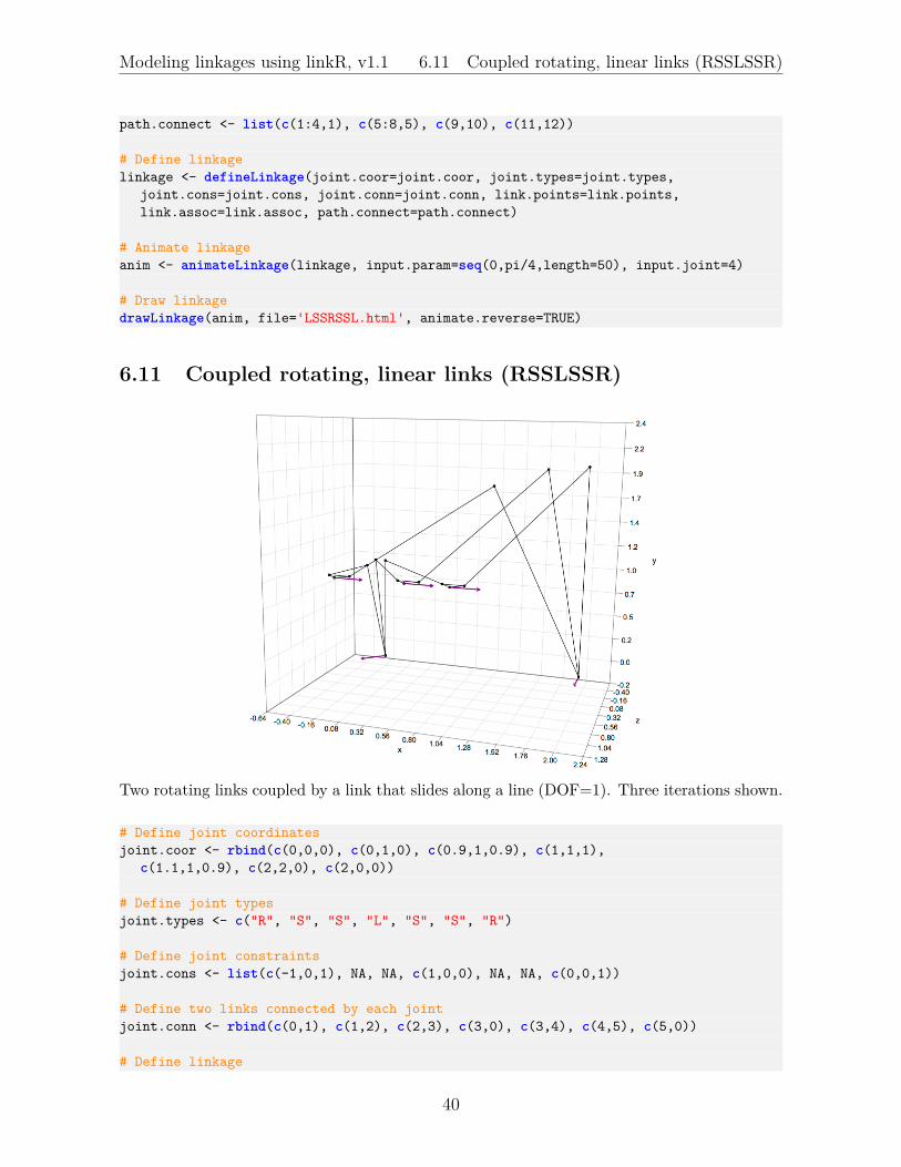
6.11 Coupled rotating, linear links (RSSLSSR)

Two rotating links coupled by a link that slides along a line (DOF=1). Three iterations shown.

# Define joint coordinatesjoint.coor <- rbind(c(0,0,0), c(0,1,0), c(0.9,1,0.9), c(1,1,1),

c(1.1,1,0.9), c(2,2,0), c(2,0,0))

# Define joint typesjoint.types <- c("R", "S", "S", "L", "S", "S", "R")

# Define joint constraintsjoint.cons <- list(c(-1,0,1), NA, NA, c(1,0,0), NA, NA, c(0,0,1))


# Define linkage

40

Modeling linkages using linkR, v1.1 6.12 Coupled rotating, planar links (RSSRSSPSS)

linkage <- defineLinkage(joint.coor=joint.coor, joint.types=joint.types,joint.cons=joint.cons, joint.conn=joint.conn)


# Draw linkagedrawLinkage(anim, file='RSSLSSR.html', animate.reverse=TRUE)

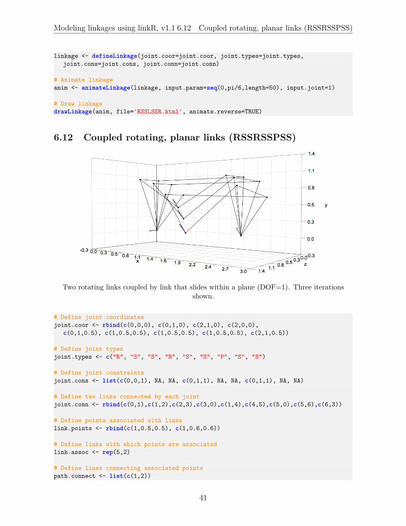
6.12 Coupled rotating, planar links (RSSRSSPSS)

Two rotating links coupled by link that slides within a plane (DOF=1). Three iterationsshown.

# Define joint coordinatesjoint.coor <- rbind(c(0,0,0), c(0,1,0), c(2,1,0), c(2,0,0),

c(0,1,0.5), c(1,0.5,0.5), c(1,0.5,0.5), c(1,0.5,0.5), c(2,1,0.5))

# Define joint typesjoint.types <- c("R", "S", "S", "R", "S", "S", "P", "S", "S")

# Define joint constraintsjoint.cons <- list(c(0,0,1), NA, NA, c(0,1,1), NA, NA, c(0,1,1), NA, NA)

# Define two links connected by each jointjoint.conn <- rbind(c(0,1),c(1,2),c(2,3),c(3,0),c(1,4),c(4,5),c(5,0),c(5,6),c(6,3))

# Define points associated with linkslink.points <- rbind(c(1,0.5,0.5), c(1,0.6,0.6))

# Define links with which points are associatedlink.assoc <- rep(5,2)

# Define lines connecting associated pointspath.connect <- list(c(1,2))

41

Modeling linkages using linkR, v1.1 6.13 Two 3D 4-bars in series (RSSRSSR))



# Animate linkageanim <- animateLinkage(linkage, input.param=seq(-0.05,-pi/4,length=50), input.joint=1)

# Draw linkagedrawLinkage(anim, file='RSSRSSPSS.html', animate.reverse=TRUE)

6.13 Two 3D 4-bars in series (RSSRSSR))

Two 3D 4-bar linkages coupled via a shared rotating link (DOF=1). Three iterations shown.

# Define joint coordinatesjoint.coor <- rbind(c(0,0,0), c(0,1,0), c(1,1,0), c(1,0,0), c(1,0.75,0), c(2,0.75,0),

c(2,0,0))

# Define joint typesjoint.types <- c("R", "S", "S", "R", "S", "S", "R")

# Define joint constraintsjoint.cons <- list(c(0.5,0,1), NA, NA, c(0,0,1), NA, NA, c(-0.5,0,1))


# Define points associated with linkslink.points <- rbind(c(0,0.5,0), c(0.5,1,0), c(1,0.5,0), c(1.5,0.75,0), c(2,0.375,0))

# Define links with which points are associatedlink.assoc <- c(1,2,3,4,5)

42

Modeling linkages using linkR, v1.1 6.14 Slider, 3D 4-bar in series (RSSR(SSL))


joint.cons=joint.cons, joint.conn=joint.conn, link.points=link.points,link.assoc=link.assoc)

# Animate linkageanim <- animateLinkage(linkage, input.param=seq(0, pi/4, length=50), input.joint=1)

# Draw linkagedrawLinkage(anim, file='RSSRSSR.html', animate=TRUE, animate.reverse=TRUE)

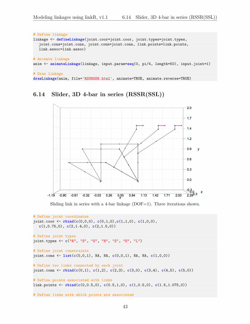
6.14 Slider, 3D 4-bar in series (RSSR(SSL))

Sliding link in series with a 4-bar linkage (DOF=1). Three iterations shown.

# Define joint coordinatesjoint.coor <- rbind(c(0,0,0), c(0,1,0),c(1,1,0), c(1,0,0),

c(1,0.75,0), c(2,1.4,0), c(2,1.5,0))

# Define joint typesjoint.types <- c("R", "S", "S", "R", "S", "S", "L")



# Define points associated with linkslink.points <- rbind(c(0,0.5,0), c(0.5,1,0), c(1,0.5,0), c(1.5,1.075,0))

# Define links with which points are associated

43

Modeling linkages using linkR, v1.1 6.15 Slider, 2D 4-bar in series (R(SSL)SSR)

link.assoc <- c(1,2,3,4)



# Animate linkageanim <- animateLinkage(linkage, input.param=seq(0, pi/3, length=50), input.joint=1)

# Draw linkagedrawLinkage(anim, file='RSSR(SSL).html', animate.reverse=TRUE)

6.15 Slider, 2D 4-bar in series (R(SSL)SSR)

Sliding link in series with a 4-bar linkage (DOF=1). Three iterations shown.

# Define joint coordinatesjoint.coor <- rbind(c(-0.5,0,0), c(0,0.6,0), c(1,1.2,0), c(1,0,0),

c(-0.5,0.7,0), c(-1,1.4,0.5), c(-1,1.5,0.5))


# Define joint constraintsjoint.cons <- list(c(0,0,-1), NA, NA, c(1,0,-1), NA, NA, c(1,0,0))


# Define points associated with linkslink.points <- rbind(c(-0.25,0.65,0), c(0.25,0.75,0), c(-0.75,1.05,0.25))

44

Modeling linkages using linkR, v1.1 6.16 Slider in parallel with 4-bar (RS(SSL)SR)

# Define links with which points are associatedlink.assoc <- c(1,2,4)




# Draw linkagedrawLinkage(anim, file='R(SSL)SSR.html', animate.reverse=TRUE)

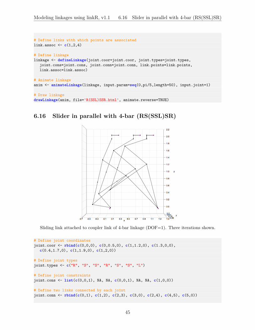
6.16 Slider in parallel with 4-bar (RS(SSL)SR)

Sliding link attached to coupler link of 4-bar linkage (DOF=1). Three iterations shown.

# Define joint coordinatesjoint.coor <- rbind(c(0,0,0), c(0,0.5,0), c(1,1.2,0), c(1.3,0,0),

c(0.4,1.7,0), c(1,1.9,0), c(1,2,0))




45

Modeling linkages using linkR, v1.1 6.17 Fish cranial joint configuration

# Define points associated with linkslink.points <- rbind(c(0.2,1.1,0), c(0.5,0.85,0))

# Define links with which points are associatedlink.assoc <- c(2,2)



# Animate linkageanim <- animateLinkage(linkage, input.param=seq(0,1.4,length=50), input.joint=1)

# Draw linkagedrawLinkage(anim, file='RS(SSL)SR.html', animate.reverse=TRUE)

6.17 Fish cranial joint configuration

A linkage based on the joint configuration (simplified) of a salmon skull (DOF=3). Threeiterations shown.

# Define joint coordinatesjoint.coor <- rbind(c(-1,1,0), c(0,1,1), c(0,1,-1), c(0,0,1.5), c(0,-1,0.1),

c(0,-1,0), c(0,-1,-0.1), c(0,0,-1.5), c(0.5,0,1.5), c(1,-0.5,0.1), c(1,-0.5,0),c(1,-0.5,-0.1), c(0.5,0,-1.5), c(0,-1,0), c(1,-0.5,0))

# Define joint typesjoint.types <- c("R","R","R","S","S","P","S","S","S","S","P","S","S","S","S")

# Define joint constraints

46

Modeling linkages using linkR, v1.1 6.17 Fish cranial joint configuration

joint.cons <- list(c(0,0,1), c(1,0,0), c(1,0,0), NA, NA, c(0,0,1), NA, NA, NA, NA,c(0,0,1), NA, NA, NA, NA)

# Define two links connected by each jointjoint.conn <- rbind(c(0,1), c(1,2), c(1,3), c(2,4), c(4,5), c(5,0), c(5,6),

c(6,3), c(2,7), c(7,9), c(9,0), c(9,8), c(8,3), c(5,10), c(10,9))

# Define points associated with linkslink.points <- rbind(c(-0.5,1,0.5), c(0,1,0), c(-0.5,1,-0.5),

c(0,0.5,1.25), c(0.25,0.5,1.25),c(0,0.5,-1.25), c(0.25,0.5,-1.25))

# Define links with which points are associatedlink.assoc <- c(rep(1,3),2,2,3,3)

# Define input parametersn_iter <- 50input.param <- list(seq(0*(pi/180), 10*(pi/180), length=n_iter),

matrix(c(-1,0,0), nrow=n_iter, ncol=3, byrow=TRUE)*matrix(seq(0, 1, length=n_iter),nrow=n_iter, ncol=3))

# Define input joint(s)input.joint <- c(1,6)



# Animate linkageanim <- animateLinkage(linkage, input.param=input.param, input.joint=input.joint)

# Draw linkagedrawLinkage(anim, file='RRRSSPSSSSPSSSS.html', animate.reverse=TRUE)

47

Modeling linkages using linkR, v1.1 6.18 Bird cranial linkage

6.18 Bird cranial linkage

The kinetic bones of a Great Horned Owl skull (Bubo virginianus) modeled as a linkagemechanism (DOF=1). Three iterations shown.

# Get specimen dataowl <- linkR_data('owl')

# Copy landmarks for easy referencelms <- owl$landmarks

# Define joint coordinatesjoint.coor <- lms[c('nc_qd_l_R', 'ju_qd_R', 'ju_ub_R', 'nc_ub_R', 'pt_qd_R',

'pa_pt_R', 'pa_pt_R', 'pa_pt_R', 'pa_ub_R', 'nc_qd_l_L', 'ju_qd_L', 'ju_ub_L','nc_ub_L', 'pt_qd_L', 'pa_pt_L', 'pa_pt_L', 'pa_pt_L', 'pa_ub_L'), ]

# Define joint typesjoint.types <- c("R", "S", "S", "R", "S", "S", "P", "S", "S",

"R", "S", "S", "R", "S", "S", "P", "S", "S")

# Define joint constraintsjoint.cons <- list(

lms['nc_qd_l_R', ]-lms['nc_qd_m_R', ], NA, NA, lms['nc_ub_L', ]-lms['nc_ub_R', ],NA, NA, lms['nc_ub_L', ]-lms['nc_ub_R', ], NA, NA,lms['nc_qd_l_L', ]-lms['nc_qd_m_L', ], NA, NA, lms['nc_ub_R', ]-lms['nc_ub_L', ],NA, NA, lms['nc_ub_R', ]-lms['nc_ub_L', ], NA, NA)

# Define two links connected by each jointjoint.conn <- rbind(

c('neurocranium', 'quadrate_R'), c('quadrate_R', 'jugal_R'),c('jugal_R', 'upperbeak'), c('upperbeak', 'neurocranium'),c('quadrate_R', 'pterygoid_R'), c('pterygoid_R', 'pp-slide_R'),

48

Modeling linkages using linkR, v1.1 6.19 Fish cranial linkage

c('pp-slide_R', 'neurocranium'), c('pp-slide_R', 'palatine_R'),c('palatine_R', 'upperbeak'), c('neurocranium', 'quadrate_L'),c('quadrate_L', 'jugal_L'), c('jugal_L', 'upperbeak'),c('upperbeak', 'neurocranium'), c('quadrate_L', 'pterygoid_L'),c('pterygoid_L', 'pp-slide_L'), c('pp-slide_L', 'neurocranium'),c('pp-slide_L', 'palatine_L'), c('palatine_L', 'upperbeak')

)

# Define points associated with linkslink.points <- owl$landmarks

# Define links with which points are associatedlink.assoc <- owl$lm.assoc

# Define lines connecting associated pointspath.connect <- owl$path.connect


joint.cons=joint.cons, link.points=link.points, link.assoc=link.assoc,joint.conn=joint.conn, path.connect=path.connect, ground.link='neurocranium')

# Animate linkageanim <- animateLinkage(linkage, input.param=seq(-0.07,0.17,length=30), input.joint=1)

# Draw linkagedrawLinkage(anim, file='owl.html', animate.reverse=TRUE)

6.19 Fish cranial linkage

The kinetic bones of an Atlantic salmon skull (Salmo salar) modeled as a linkage mechanism

49


(DOF=3). Three iterations shown.

# Get specimen datasalmon <- linkR_data('salmon')

# Copy landmarks for easy referencelms <- salmon$landmarks

# Define joint coordinatesjoint.coor <- lms[c('nc_vc', 'nc_su_a_L', 'pc_su_L', 'ac_hy_L', 'hy_mid',

'ac_hy_R', 'pc_su_R', 'nc_su_a_R', 'hy_mid', 'lj_sy_inf', 'lj_sy_inf','lj_qd_L', 'lj_sy_inf', 'lj_sy_inf', 'lj_qd_R'), ]

# Define joint typesjoint.types <- c("R","R","S","S","P","S","S","R","S","S","P","S","S","S","S")

# Define joint constraintsjoint.cons <- list(

lms['nc_su_p_L', ] - lms['nc_su_p_R', ], lms['nc_su_a_L', ] - lms['nc_su_p_L', ],NA, NA, lms['nc_su_a_L', ] - lms['nc_su_a_R', ], NA, NA,lms['nc_su_a_R', ] - lms['nc_su_p_R', ], NA, NA,lms['nc_su_a_L', ] - lms['nc_su_a_R', ], NA, NA, NA, NA)

# Define two links connected by each jointjoint.conn <- rbind(

c('vert_column', 'neurocranium'), c('neurocranium', 'suspensorium_L'),c('suspensorium_L', 'hyoid_L'), c('hyoid_L', 'hypohyal'),c('hypohyal', 'vert_column'), c('hypohyal', 'hyoid_R'),c('hyoid_R', 'suspensorium_R'), c('suspensorium_R', 'neurocranium'),c('hypohyal', 'hyoid_lowerjaw'), c('hyoid_lowerjaw', 'lowerjaw_symph'),c('lowerjaw_symph', 'vert_column'), c('suspensorium_L', 'lowerjaw_L'),c('lowerjaw_L', 'lowerjaw_symph'), c('lowerjaw_symph', 'lowerjaw_R'),c('lowerjaw_R', 'suspensorium_R'))

# Set long axis rotation constraintslar.cons <- list(

list('link'='lowerjaw_L', 'type'='P', 'point'=lms['lj_sy_sup', ],'vec'=lms['nc_su_p_L', ] - lms['nc_su_p_R', ]),

list('link'='lowerjaw_R', 'type'='P', 'point'=lms['lj_sy_sup', ],'vec'=lms['nc_su_p_L', ] - lms['nc_su_p_R', ]),

list('link'='hyoid_R', 'type'='P', 'point'=lms['ac_as_R', ],'vec'=lms['nc_su_p_L', ] - lms['nc_su_p_R', ]),

list('link'='hyoid_L', 'type'='P', 'point'=lms['ac_as_L', ],'vec'=lms['nc_su_p_L', ] - lms['nc_su_p_R', ]))

# Define points associated with linkslink.points <- salmon$landmarks

# Define links with which points are associatedlink.assoc <- salmon$lm.assoc

# Define lines connecting associated pointspath.connect <- salmon$path.connect

50



joint.cons=joint.cons, link.points=link.points, link.assoc=link.assoc,joint.conn=joint.conn, path.connect=path.connect, ground.link='vert_column',lar.cons=lar.cons)

# Set number of animation iterationsanim_len <- 9

# Set input parametersinput.param <- list(seq(0,-0.1,length=anim_len),

cbind(seq(0.001,-3.001,length=anim_len), rep(0, anim_len), rep(0, anim_len)))

# Animate linkage (this can take some time to run)anim <- animateLinkage(linkage, input.param=input.param, input.joint=c(1,5))

# Draw linkagedrawLinkage(anim, file='salmon.html', animate.reverse=TRUE)

51

Modeling linkages using linkR, v1.1 7 Citing linkR

7 Citing linkRThe linkR R package are the result of several years of work. I am pleased to offer thesoftware open-source and free of charge and hope that users find it useful and that itbrings about interesting, fruitful and fun advances for biologists and non-biologists alike.I only ask that if you use linkR and share your results that you include a citation. Forpeer-reviewed publications, please cite the following article:

Olsen, A.M. and Westneat, M.W. (2016). Linkage mechanisms in the vertebrate skull:Structure and function of three-dimensional, parallel transmission systems. Journal ofMorphology. Early View. DOI: 10.1002/jmor.20596.

8 AcknowledgementsI would like to thank Mark Westneat, whose previous work modeling cranial kinesis infishes and birds using linkage mechanisms inspired the development of the linkR package.linkR was developed as we worked together applying three-dimensional linkage modelsto the kinetic mechanisms of fish and bird skulls. The software benefitted greatly fromthese collaborations and will continue to benefit from ongoing and future collaborations. Iwould also like to thank Michael Coates, whose invitation to collaborate in modeling earlychondrichthyan jaw linkages using the first version of linkR instigated the application oflinkR to modeling buccal expansion in fishes. Thank you to Dave Willard, Ben Marksand Mary Hennen in the Bird Division at the Field Museum of Natural History foraccommodating access to fresh and skeletal specimens. The development of linkR wasmade possible by funding from the US National Science Foundation (DGE-1144082;DGE-0903637; DBI-1612230).

52


modeling linkages in r using linkr - aaron olsen linkages using... · modeling linkages in r using...

Documents