GNU Linear Programming Kit

Modeling Language GNU MathProg

Version 4.1

(Draft Edition, August 2003)

2

The GLPK package is a part of the GNU project released under the aegis of GNU.

Copyright c© 2000, 2001, 2002, 2003 Andrew Makhorin, Department for Applied Infor-matics, Moscow Aviation Institute, Moscow, Russia. All rights reserved.

Free Software Foundation, Inc., 59 Temple Place — Suite 330, Boston, MA 02111, USA.

Permission is granted to make and distribute verbatim copies of this manual provided thecopyright notice and this permission notice are preserved on all copies.

Permission is granted to copy and distribute modified versions of this manual under theconditions for verbatim copying, provided also that the entire resulting derived work isdistributed under the terms of a permission notice identical to this one.

Permission is granted to copy and distribute translations of this manual into anotherlanguage, under the above conditions for modified versions.

3

Contents

4

1 Introduction

GNU MathProg is a modeling language intended for describing linear mathematical pro-gramming models.1

Model descriptions written in the GNU MathProg language consist of a set of state-ments and data blocks constructed by the user from the language elements described inthis document.

In a process called translation, a program called the model translator analyzes themodel description and translates it into internal data structures, which may be then usedeither for generating mathematical programming problem instance or directly by a pro-gram called the solver to obtain numeric solution of the problem.

1.1 Linear programming problem

In MathProg the following formulation of linear programming (LP) problem is assumed:

minimize (maximize)

Z = c1xm+1 + c2xm+2 + . . . + cnxm+n + c0 (1)

subject to linear constraints

x1 = a11xm+1 + a12xm+2 + . . . + a1nxm+n

x2 = a21xm+1 + a22xm+2 + . . . + a2nxm+n

. . . . . . . . . . . . . . . . . .xm = am1xm+1 + am2xm+2 + . . . + amnxm+n

(2)

and bounds of variables

l1 ≤ x1 ≤ u1

l2 ≤ x2 ≤ u2

. . . . . . . . .lm+n ≤ xm+n ≤ um+n

(3)

where: x1, x2, . . . , xm are auxiliary variables; xm+1, xm+2, . . . , xm+n are structural vari-ables; Z is the objective function; c1, c2, . . . , cn are coefficients of the objective function;c0 is the constant term of the objective function; a11, a12, . . . , amn are constraint coeffi-cients; l1, l2, . . . , lm+n are lower bounds of variables; u1, u2, . . . , um+n are upper bounds ofvariables.

Bounds of variables can be finite as well as infinite. Besides, lower and upper boundscan be equal to each other. Thus, the following types of variables are possible:

Bounds of variable Type of variable−∞ < xk < +∞ Free (unbounded) variable

lk ≤ xk < +∞ Variable with lower bound−∞ < xk ≤ uk Variable with upper bound

lk ≤ xk ≤ uk Double-bounded variablelk = xk = uk Fixed variable

Note that the types of variables shown above are applicable to structural as well as toauxiliary variables.

In addition to pure LP problems MathProg allows mixed integer linear programming(MIP) problems, where some (or all) structural variables are restricted to be integer.

1The GNU MathProg language is a subset of the AMPL language.

5

1.2 Model objects

In MathProg the model is described in terms of sets, parameters, variables, constraints,and objectives, which are called model objects.

The user introduces particular model objects using the language statements. Eachmodel object is provided with a symbolic name that uniquely identifies the object and isintended for referencing purposes.

Model objects, including sets, can be multidimensional arrays built over indexing sets.Formally, n-dimensional array A is the mapping

A : ∆ → Ξ, (4)

where ∆ ⊆ S1 × S2 × . . .× Sn is a subset of the Cartesian product of indexing sets, Ξ is aset of the array members. In MathProg the set ∆ is called subscript domain. Its membersare n-tuples (i1, i2, . . . , in), where i1 ∈ S1, i2 ∈ S2, . . . , in ∈ Sn.

If n = 0, the Cartesian product in (4) has exactly one element (namely, 0-tuple), so itis convenient to think scalar objects as 0-dimensional arrays that have one member.

The type of array members is determined by the type of the corresponding modelobject as follows:

Model object Array memberSet Elemental plain setParameter Number or symbolVariable Elemental structural variableConstraint Elemental constraintObjective Elemental objective

In order to refer to a particular object member the object should be provided withsubscripts. For example, if a is 2-dimensional parameter built over I × J , a reference toits particular member can be written as a[i, j], where i ∈ I and j ∈ J . It is understoodthat scalar objects being 0-dimensional need no subscripts.

1.3 Structure of model description

It is sometimes desirable to write a model which, at various points, may require differentdata for each problem to be solved using that model. For this reason in MathProg themodel description consists of two parts: model section and data section.

Model section is a main part of the model description that contains declarations ofmodel objects and is common for all problems based on the corresponding model.

Data section is an optional part of the model description that contains data specificfor a particular problem.

Depending on what is more convenient model and data sections can be placed eitherin one file or in two separate files. The latter feature allows to have arbitrary number ofdifferent data sections to be used with the same model section.

6

2 Coding model description

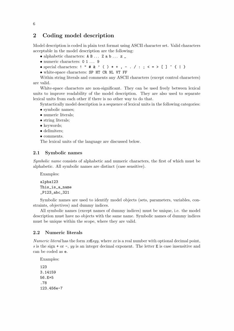
Model description is coded in plain text format using ASCII character set. Valid charactersacceptable in the model description are the following:

• alphabetic characters: A B . . . Z a b . . . z _• numeric characters: 0 1 . . . 9• special characters: ! " # & ’ ( ) * + , - . / : ; < = > [ ] ^ { | }• white-space characters: SP HT CR NL VT FFWithin string literals and comments any ASCII characters (except control characters)

are valid.White-space characters are non-significant. They can be used freely between lexical

units to improve readability of the model description. They are also used to separatelexical units from each other if there is no other way to do that.

Syntactically model description is a sequence of lexical units in the following categories:• symbolic names;• numeric literals;• string literals;• keywords;• delimiters;• comments.The lexical units of the language are discussed below.

2.1 Symbolic names

Symbolic name consists of alphabetic and numeric characters, the first of which must bealphabetic. All symbolic names are distinct (case sensitive).

Examples:

alpha123This_is_a_name_P123_abc_321

Symbolic names are used to identify model objects (sets, parameters, variables, con-straints, objectives) and dummy indices.

All symbolic names (except names of dummy indices) must be unique, i.e. the modeldescription must have no objects with the same name. Symbolic names of dummy indicesmust be unique within the scope, where they are valid.

2.2 Numeric literals

Numeric literal has the form xxEsyy, where xx is a real number with optional decimal point,s is the sign + or -, yy is an integer decimal exponent. The letter E is case insensitive andcan be coded as e.

Examples:

1233.1415956.E+5.78123.456e-7

7

Numeric literals are used to represent numeric quantities. They have obvious fixedmeaning.

2.3 String literals

String literal is a sequence of arbitrary characters enclosed either in single quotes or indouble quotes. Both these forms are equivalent.

If the single quote is a part of a string literal enclosed in single quotes, it must becoded twice. Analogously, if the double quote is a part of string literal enclosed in doublequotes, it must be coded twice.

Examples:

’This is a string’"This is another string"’1 + 2 = 3’’That’’s all’"She said: ""No"""

String literals are used to represent symbolic quantities.

2.4 Keywords

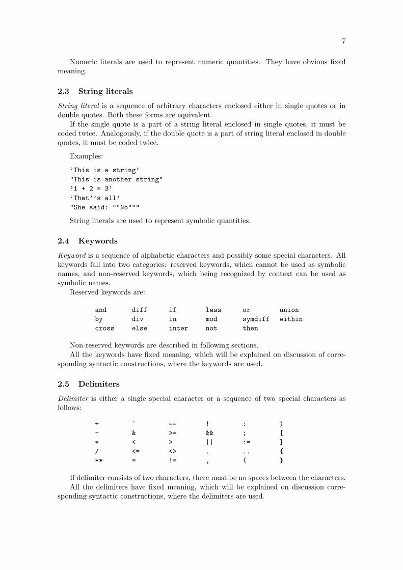
Keyword is a sequence of alphabetic characters and possibly some special characters. Allkeywords fall into two categories: reserved keywords, which cannot be used as symbolicnames, and non-reserved keywords, which being recognized by context can be used assymbolic names.

Reserved keywords are:

and diff if less or unionby div in mod symdiff withincross else inter not then

Non-reserved keywords are described in following sections.All the keywords have fixed meaning, which will be explained on discussion of corre-

sponding syntactic constructions, where the keywords are used.

2.5 Delimiters

Delimiter is either a single special character or a sequence of two special characters asfollows:

+ ^ == ! : )- & >= && ; [* < > || := ]/ <= <> . .. {** = != , ( }

If delimiter consists of two characters, there must be no spaces between the characters.All the delimiters have fixed meaning, which will be explained on discussion corre-

sponding syntactic constructions, where the delimiters are used.

8

2.6 Comments

For documenting purposes the model description can be provided with comments, whichhave two different forms. The first form is a single-line comment, which begins with thecharacter # and extends until end of line. The second form is a comment sequence, whichis a sequence of any characters enclosed between /* and */.

Examples:

set s{1..10}; # This is a comment/* This is another comment */

Comments are ignored by the model translator and can appear anywhere in the modeldescription, where white-space characters are allowed.

9

3 Expressions

Expression is a rule for computing a value. In model description expressions are used asconstituents of certain statements.

In general case expressions consist of operands and operators.Depending on the type of the resultant value all expressions fall into the following

categories:• numeric expressions;• symbolic expressions;• indexing expressions;• set expressions;• logical expressions;• linear expressions.

3.1 Numeric expressions

Numeric expression is a rule for computing a single numeric value represented in the formof floating-point number.

The primary numeric expression may be a numeric literal, dummy index, unsubscriptedparameter, subscripted parameter, built-in function reference, iterated numeric expression,conditional numeric expression, or another numeric expression enclosed in parentheses.

Examples:

1.23 numeric literalj dummy indextime unsubscripted parametera[’May 2003’,j+1] subscripted parameterabs(b[i,j]) function referencesum{i in S diff T} alpha[i] * b[i,j] iterated expressionif i in I and p >= 1 then 2 * p else q[i+1] conditional expression(b[i,j] + .5 * c) parenthesized expression

More general numeric expressions containing two or more primary numeric expressionsmay be constructed by using certain arithmetic operators.

Examples:

j+12 * a[i-1,j+1] - b[i,j]sum{j in J} a[i,j] * x[j] + sum{k in K} b[i,k] * x[k](if i in I and p >= 1 then 2 * p else q[i+1]) / (a[i,j] + 1.5)

Numeric literals. If the primary numeric expression is a numeric literal, the resultantvalue is obvious.

Dummy indices. If the primary numeric expression is a dummy index, the resultantvalue is current value assigned to the dummy index.

Unsubscripted parameters. If the primary numeric expression is an unsubscriptedparameter (which must be 0-dimensional), the resultant value is the value of the parameter.

10

Subscripted parameters. The primary numeric expression, which refers to a sub-scripted parameter, has the following syntactic form:

name[i1,i2, . . . ,in]

where name is the symbolic name of the parameter, i1, i2, . . . , in are subscripts.Each subscript must be a numeric or symbolic expression. The number of subscripts

in the subscript list must be the same as the dimension of the parameter with which thesubscript list is associated.

Actual values of subscript expressions are used to identify a particular member of theparameter that determines the resultant value of the primary expression.

Function references. In MathProg there are the following built-in functions that maybe used in numeric expressions:

abs(x) absolute valueceil(x) smallest integer not less than x (“ceiling of x”)floor(x) largest integer not greater than x (“floor of x”)exp(x) base-e exponential ex

log(x) natural logarithm log xlog10(x) common (decimal) logarithm log10 xmax(x1, x2, . . . , xn) the largest of values x1, x2, . . . , xn

min(x1, x2, . . . , xn) the smallest of values x1, x2, . . . , xn

sqrt(x) square root√

x

All the built-in functions, except min and max, require one argument, which must benumeric expression. The functions min and max allow arbitrary number of arguments,which all must be numeric expressions.

The resultant value of the numeric expression, which is a function reference, is theresult of applying the function to its argument(s).

Iterated expressions. Iterated numeric expression is a primary numeric expression,which has the following syntactic form:

iterated-operator indexing-expression integrand

where iterated-operator is the symbolic name of the iterated operator to be performed (seebelow), indexing expression is an indexing expression that introduces dummy indices andcontrols iterating, integrand is a numeric expression that participates in the operation.

In MathProg there are four iterated operators, which may be used in numeric expres-sions:

sum summation∑

(i1,...,in)∈∆ x(i1, . . . , in)

prod production∏

(i1,...,in)∈∆ x(i1, . . . , in)

min minimum min(i1,...,in)∈∆ x(i1, . . . , in)

max maximum max(i1,...,in)∈∆ x(i1, . . . , in)

11

where i1, . . . , in are dummy indices introduced in the indexing expression, ∆ is the domain,a set of n-tuples specified by the indexing expression that defines particular values assignedto the dummy indices on performing the iterated operation, x(i1, . . . , in) is the integrand,a numeric expression whose resultant value depends on the dummy indices.

The resultant value of an iterated numeric expression is the result of applying of theiterated operator to its integrand over all n-tuples contained in the domain.

Conditional expressions. Conditional numeric expression is a primary numeric ex-pression, which has the following two syntactic forms:

if b then x else yif b then x

where b is an logical expression, x and y are numeric expressions.The resultant value of the conditional expression depends on the value of the logical

expression that follows the keyword if. If it is true, the value of the conditional expressionis the value of the expression that follows the keyword then. Otherwise, if the logicalexpression has the value false, the value of the conditional expression is the value of theexpression that follows the keyword else. If the reduced form of the conditional expressionis used and the logical expression has the value false, the resultant value of the conditionalexpression is zero.

Parenthesized expressions. Any numeric expression may be enclosed in parenthesesthat syntactically makes it primary numeric expression.

Parentheses may be used in numeric expressions, as in algebra, to specify the desiredorder in which operations are to be performed. Where parentheses are used, the expressionwithin the parentheses is evaluated before the resultant value is used.

The resultant value of the parenthesized expression is the same as the value of theexpression enclosed within parentheses.

Arithmetic operators. In MathProg there are the following arithmetic operators,which may be used in numeric expressions:

+ x unary plus- x unary minusx + y additionx - y subtractionx less y positive difference (if x < y then 0 else x− y)x * y multiplicationx / y divisionx div y quotient of exact divisionx mod y remainder of exact divisionx ** y, x ^ y exponentiation (raise to power)

where x and y are numeric expressions.If the expression includes more than one arithmetic operator, all operators are per-

formed from left to right according to the hierarchy of operations (see below) with theonly exception that the exponentiaion operators are performed from right to left.

The resultant value of the expression, which contains arithmetic operators, is the resultof applying the operators to their operands.

12

Hierarchy of operations. The following list shows the hierarchy of operations in nu-meric expressions:

Operation HierarchyEvaluation of functions (abs, ceil, etc.) 1stExponentiation (**, ^) 2ndUnary plus and minus (+, -) 3rdMultiplication and division (*, /, div, mod) 4thIterated operations (sum, prod, min, max) 5thAddition and subtraction (+, -, diff) 6thConditional evaluation (if . . . then . . . else) 7th

This hierarchy is used to determine which of two consecutive operations is performedfirst. If the first operator is higher than or equal to the second, the first operation isperformed. If it is not, the second operator is compared to the third, etc. When the endof the expression is reached, all of the remaining operations are performed in the reverseorder.

3.2 Symbolic expressions

Symbolic expression is a rule for computing a single symbolic value represented in the formof character string.

The primary symbolic expression may be a string literal, dummy index, unsubscriptedparameter, subscripted parameter, conditional symbolic expression, or another symbolicexpression enclosed in parentheses.

It is also allowed to use a numeric expression as the primary symbolic expression, inwhich case the resultant value of the numeric expression is automatically converted to thesymbolic type.

Examples:

’May 2003’ string literalj dummy indexp unsubscripted parameters[’abc’,j+1] subscripted parameterif i in I then s[i,j] & "..." else t[i+1] conditional expression((10 * b[i,j]) & ’.bis’) parenthesized expression

More general symbolic expressions containing two or more primary symbolic expres-sions may be constructed by using the concatenation operator.

Examples:

’abc[’ & i & ’,’ & j & ’]’"from " & city[i] " to " & city[j]

The principles of evaluation of symbolic expressions are entirely analogous to that thatgiven for numeric expressions (see above).

Symbolic operators. Currently in MathProg there is the only symbolic operator:

x & y

where x and y are symbolic expressions. This operator means concatenation of its twosymbolic operands, which are character strings.

13

Hierarchy of operations The following list shows the hierarchy of operations in sym-bolic expressions:

Operation HierarchyEvaluation of numeric operations 1st-7thConcatenation (&) 8thConditional evaluation (if . . . then . . . else) 9th

This hierarchy has the same meaning as explained in Subsection “Numeric expressions”.

3.3 Indexing expressions and dummy indices

Indexing expression is an auxiliary construction, which specifies a plain set of n-tuples andintroduces dummy indices. It has two syntactic forms:

{entry1, entry2, . . . , entrym}{entry1, entry2, . . . , entrym : predicate}

(5)

where entry1, entry2, . . . , entrym are indexing entries, predicate is a logical expression thatspecifies optional predicate.

Each indexing entry in the indexing expression have the following three forms:

t in S(t1, t2, . . . , tk) in SS

(6)

where t, t1, t2, . . . , tk are indices, S is a set expression that specifies the basic set.The number of indices in the indexing entry must be the same as the dimension of the

basic set S, i.e. if S consists of 1-tuples, the first form must be used, and if S consists ofn-tuples, where n > 1, the second form must be used.

If the first form of the indexing entry is used, the index t can be a dummy index only.If the second form is used, the indices t1, t2, . . . , tk can be either dummy indices or somenumeric or symbolic expressions, where at least one index must be a dummy index. Thethird, reduced form of the indexing entry has the same effect as if there were t (if S is1-dimensional) or t1, t2, . . . , tk (if S is n-dimensional) all specified as dummy indices.

Dummy index is an auxiliary model object, which acts like an individual variable.Values assigned to dummy indices are components of n-tuples from basic sets, i.e. somenumeric and symbolic quantities.

For referencing purposes dummy indices can be provided with symbolic names. How-ever, unlike other model objects (sets, parameters, etc.) dummy indices don’t need tobe explicitly declared. Each undeclared symbolic name being used in indexing position ofsome indexing entry is recognized as symbolic name of corresponding dummy index.

Symbolic names of dummy indices are valid only within the scope of the indexingexpression, where the dummy indices were introduced. Beyond the scope the dummyindices are completely inaccessible, so the same symbolic names may be used for otherpurposes, in particular, to represent dummy indices in other indexing expressions.

The scope of indexing expression, where implicit declarations of dummy indices arevalid, depends on the context, in which the indexing expression is used:

14

1. If the indexing expression is used in iterated operator, its scope extends until theend of the integrand.

2. If the indexing expression is used as a primary set expression, its scope extends untilthe end of this indexing expression.

3. If the indexing expression is used to define the subscript domain in declarations ofsome model objects, its scope extends until the end of the corresponding statement.

The indexing mechanism implemented by means of indexing expressions is best ex-plained by some examples discussed below.

Let there be three sets:

A = {4, 7, 9}B = {(1, Jan), (1, F eb), (2,Mar), (2, Apr), (3,May), (3, Jun)}C = {a, b, c}

(7)

where A and B consist of 1-tuples (singles), C consists of 2-tuples (doubles). And considerthe following indexing expression:

{i in A, (j,k) in B, l in C} (8)

where i, j, k, and l are dummy indices.Although MathProg is not a procedural language, for any indexing expression an

equivalent algorithmic description can be given. In particular, the algorithmic descriptionof the indexing expression (8) is the following:

for all i ∈ A dofor all (j, k) ∈ B do

for all l ∈ C doaction;

where the dummy indices i, j, k, l are consecutively assigned corresponding componentsof n-tuples from the basic sets A, B, C, and action is some action that depends on thecontext, where the indexing expression is used. For example, if the action were printingcurrent values of dummy indices, the output would look like follows:

i = 4 j = 1 k = Jan l = ai = 4 j = 1 k = Jan l = bi = 4 j = 1 k = Jan l = ci = 4 j = 1 k = Feb l = ai = 4 j = 1 k = Feb l = b. . . . . . . . . . . .

i = 9 j = 3 k = Jun l = bi = 9 j = 3 k = Jun l = c

Let the indexing expression (8) be used in the following iterated operation:

sum{i in A, (j,k) in B, l in C} p[i,j,k,l] ** 2 (9)

where p[i, j, k, l] may be a 4-dimensional numeric parameter or some numeric expressionwhose resultant value depends on i, j, k, and l. In this case the action is summation, sothe resultant value of the primary numeric expression (9) is:∑

i∈A,(j,k)∈B,l∈C

(pijkl)2.

15

Now let the indexing expression (8) be used as a primary set expression. In this casethe action is gathering all 4-tuples (quadruples) of the form (i, j, k, l) in one set, so theresultant value of such operation is simply the Cartesian product of the basic sets:

A×B × C = {(i, j, k, l)|i ∈ A, (j, k) ∈ B, l ∈ C}.

Note that in this case the same indexing expression might be written in the reduced form:

{A, B, C}

because the dummy indices i, j, k, l are not referenced and therefore their symbolic namesare not needed.

Finally, let the indexing expression (8) be used as the subscript domain in declarationof some 4-dimensional model object, for instance, some numeric parameter:

par p{i in A, (j,k) in B, l in C} ... ;

In this case the action is generating the parameter members, where each member has theform p[i, j, k, l].

As was said above, some indices in (6) may be numeric or symbolic expressions, notdummy indices. In this case resultant values of such expressions play role of some logicalconditions to select only that n-tuples from the Cartesian product of basic sets, whichsatisfy these conditions.

Consider, for example, the following indexing expression:

{i in A, (i-1,k) in B, l in C} (10)

where i, k, l are dummy indices, and i − 1 is a numeric expression. The algorithmicdecsription of the indexing expression (10) is the following:

for all i ∈ A dofor all (j, k) ∈ B and j = i− 1 do

for all l ∈ C doaction;

Thus, if the indexing expression (10) is used as a primary set expression, the resultant setis the following:

{(4,May, a), (4,May, b), (4,May, c), (4, Jun, a), (4, Jun, b), (4, Jun, c)}

Should note that in this case the resultant set consists of 3-tuples, not of 4-tuples, becausein the indexing expression (10) there is no dummy index that corresponds to the firstcomponent of 2-tuples from the set B.

The general rule is: the number of components of n-tuples defined by an indexingexpression is the same as the number of dummy indices in that indexing expression, wherethe correspondence between dummy indices and components on n-tuples in the resultantset is positional, i.e. the first dummy index corresponds to the first component, the seconddummy index corresponds to the second component, etc.

In many cases it is needed to select a subset from some set of from the Cartesianproduct of some sets. This may be attained by using an optional logical predicate, whichis specified in indexing expression after the last or the only indexing entry.

16

Consider, for example, the following indexing expression:

{i in A, (j,k) in B, l in C: i <= 5 and k <> ’Mar’} (11)

where the logical expression following the colon is a predicate. The algorithmic descriptionof this indexing expression is the following:

for all i ∈ A dofor all (j, k) ∈ B do

for all l ∈ C doif i ≤ 5 and k 6= ‘Mar’ then

action;

Thus, if the indexing expression (11) is used as a primary set expression, the resultant setis the following:

{(4, 1, Jan, a), (4, 1, F eb, a), (4, 2, Apr, a), . . . , (4, 3, Jun, c)}.

If no predicate is specified in indexing expression, one is assumed whose value is true.

3.4 Set expressions

Set expression is a rule for computing an elemental set, i.e. a collection of n-tuples, wherecomponents of n-tuples are numeric and symbolic quantities.

The primary set expression may be a literal set, unsubscripted set, subscripted set,“arithmetic” set, indexing expression, iterated set expression, conditional set expression,or another set expression enclosed in parentheses.

Examples:

{(123,’aaa’), (i+1,’bbb’), (j-1,’ccc’)} literal setI unsubscripted setS[i-1,j+1] subscripted set1..t-1 by 2 “arithmetic” set{t in 1..T, (t+1,j) in S: (t,j) in F} indexing expressionsetof{i in I, j in J}(i+1,j-1) iterated set expressionif i < j then S[i,j] else F diff S[i,j] conditional set expression(1..10 union 21..30) parenthesized set expression

More general set expressions containing two or more primary set expressions may beconstructed by using certain set operators.

Examples:

(A union B) inter (I cross J)1..10 cross (if i < j then {’a’, ’b’, ’c’} else {’d’, ’e’, ’f’})

Literal sets. Literal set is a primary set expression, which has the following two syntacticforms:

{e1,e2, . . . ,em}{(e11, . . . ,e1n),(e21, . . . ,e2n), . . . ,(em1, . . . ,emn)}

where e1, . . . , em, e11, . . . , emn are numeric or symbolic expressions.

17

If the first form is used, the resultant set consists of 1-tuples (singles) enumeratedwithin the curly braces. It is allowed to specify an empty set, which has no 1-tuples.

If the second form is used, the resultant set consists of n-tuples enumerated within thecurly braces, where a particular n-tuple consists of corresponding components enumeratedwithin the parentheses. All n-tuples must have the same number of components.

Unsubscripted set. If the primary set expression is an unsubscripted set (which mustbe 0-dimensional), the resultant set is an elemental set associated with the correspondingset object.

Subscripted set. The primary set expression, which refers to a subscripted set, has thefollowing syntactic form:

name[i1,i2, . . . ,in]

where name is the symbolic name of the set object, i1, i2, . . . , in are subscripts.Each subscript must be a numeric or symbolic expression. The number of subscripts

in the subscript list must be the same as the dimension of the set object with which thesubscript list is associated.

Actual values of subscript expressions are used to identify a particular member of theset object that determines the resultant set.

“Arithmetic” set. The primary set expression, which is an “arithmetic” set, has thefollowing two syntactic forms:

t0 .. tf by δtt0 .. tf

where t0, t1, and δt are numeric expressions (the value of δt must not be zero). The secondform is equivalent to the first form, where δt = 1.

If δt > 0, the resultant set is determined as follows:

{t : ∃k ∈ Z(t = t0 + kδt, t0 ≤ t ≤ tf )}

If δt < 0, the resultant set is determined as follows:

{t : ∃k ∈ Z(t = t0 + kδt, tf ≤ t ≤ t0)}

Indexing expressions. If the primary set expression is an indexing expression, theresultant set is determined as described in Subsection “Indexing expressions and dummyindices” (see above).

Iterated expressions. Iterated set expression is a primary set expression, which hasthe following syntactic form:

setof indexing-expression integrand

where indexing-expression is an indexing expression that introduces dummy indices andcontrols iterating, integrand is either a single numeric or symbolic expression or a list ofnumeric and symbolic expressions separated by commae and enclosed in parentheses.

18

If the integrand is a single numeric or symbolic expression, the resultant set consistsof 1-tuples and is determined as follows:

{x : (i1, . . . , in) ∈ ∆},

where x is a value of the integrand, i1, . . . , in are dummy indices introduced in the in-dexing expression, ∆ is the domain, a set of n-tuples specified by the indexing expressionthat defines particular values assigned to the dummy indices on performing the iteratedoperation.

If the integrand is a list containing m numeric and symbolic expressions, the resultantset consists of m-tuples and is determined as follows:

{(x1, . . . , xm) : (i1, . . . , in) ∈ ∆},

where x1, . . . , xm are values of the expressions in the integrand list, i1, . . . , in and ∆ havethe same meaning as above.

Conditional expressions. Conditional set expression is a primary set expression thathas the following syntactic form:

if b then X else Y

where b is an logical expression, X and Y are set expressions, which must define sets ofthe same dimension.

The resultant value of the conditional expression depends on the value of the logicalexpression that follows the keyword if. If it is true, the resultant set is the value of theexpression that follows the keyword then. Otherwise, if the logical expression has thevalue false, the resultant set is the value of the expression that follows the keyword else.

Parenthesized expressions. Any set expression may be enclosed in parentheses thatsyntactically makes it primary set expression.

Parentheses may be used in set expressions, as in algebra, to specify the desired orderin which operations are to be performed. Where parentheses are used, the expressionwithin the parentheses is evaluated before the resultant value is used.

The resultant value of the parenthesized expression is the same as the value of theexpression enclosed within parentheses.

Set operators. In MathProg there are the following set operators, which may be usedin set expressions:

X union Y union X ∪ YX diff Y difference X\YX symdiff Y symmetric difference X ⊕ YX inter Y intersection X ∩ YX cross Y cross (Cartesian) product X × Y

where X and Y are set expressions, which must define sets of the identical dimension(except for the Cartesian product).

If the expression includes more than one set operator, all operators are performed fromleft to right according to the hierarchy of operations (see below).

19

The resultant value of the expression, which contains set operators, is the result ofapplying the operators to their operands.

The dimension of the resultant set, i.e. the dimension of n-tuples, of which the resultantset consists of, is the same as the dimension of the operands except the Cartesian product,where the dimension of the resultant set is the sum of dimension of the operands.

Hierarchy of operations. The following list shows the hierarchy of operations in setexpressions:

Operation HierarchyEvaluation of numeric operations 1st-7thEvaluation of symbolic operations 8th-9thEvaluation of iterated or “arithmetic” set (setof, ..) 10thCartesian product (cross) 11thIntersection (inter) 12thUnion and difference (union, diff, symdiff) 13thConditional evaluation (if . . . then . . . else) 14th

This hierarchy is used to determine which of two consecutive operations is performed first.If the first operator is higher than or equal to the second, the first operation is performed.If it is not, the second operator is compared to the third, etc. When the end of theexpression is reached, all of the remaining operations are performed in the reverse order.

3.5 Logical expressions

Logical expression is a rule for computing a single logical value, which can be either trueor false.

The primary logical expression may be a numeric expression, relational expression,iterated logical expression, or another logical expression enclosed in parentheses.

Examples:

i+1 numeric expressiona[i,j] < 1.5 relational expressions[i+1,j-1] <> ’Mar’ & year relational expression(i+1,’Jan’) not in I cross J relational expressionS union T within A[i] inter B[j] relational expressionforall{i in I, j in J} a[i,j] < .5 * b[i] iterated logical expression(a[i,j] < 1.5 or b[i] >= a[i,j]) parenthesized logical expression

More general logical expressions containing two or more primary logical expressionsmay be constructed by using certain logical operators.

Examples:

not (a[i,j] < 1.5 or b[i] >= a[i,j]) and (i,j) in S(i,j) in S or (i,j) not in T

Numeric expressions. The resultant value of the primary logical expression, which isa numeric expression, is true if the resultant value of the numeric expression is not zero,otherwise the resultant value of the logical expression is false.

20

Relational expressions. In MathProg there are the following relational operators,which may be used in logical expressions:

x < y test on x < yx <= y test on x ≤ yx = y, x == y test on x = yx >= y test on x ≥ yx <> y, x != y test on x 6= yx in Y test on x ∈ Y(x1, . . . , xn) in Y test on (x1, . . . , xn) ∈ Yx not in Y , x !in Y test on x 6∈ Y(x1, . . . , xn) not in Y , (x1, . . . , xn) !in Y test on (x1, . . . , xn) 6∈ YX within Y test on X ⊆ YX not within Y , X !within Y test on X 6⊆ Y

where x, x1, . . . , xn, y are numeric or symbolic expressions, X and Y are set expression.Notes:1. If x and y are symbolic expressions, only the relational operators =, ==, <>, and !=

can be used.2. In the operations in, not in, and !in the number of components in the first

operands must be the same as the dimension of the second operand.3. In the operations within, not within, and !within both operands must have

identical dimension.All the relational operators have their conventional mathematical meaning. The resul-

tant value takes on the value true if the corresponding relation is satisfied for its operands,otherwise false.

Iterated expressions. Iterated logical expression is a primary logical expression, whichhas the following syntactic form:

iterated-operator indexing-expression integrand

where iterated-operator is the symbolic name of the iterated operator to be performed (seebelow), indexing expression is an indexing expression that introduces dummy indices andcontrols iterating, integrand is a logical expression that participates in the operation.

In MathProg there are two iterated operators, which may be used in logical expressions:

forall ∀-quantification ∀(i1, . . . , in)∈∆[x(i1, . . . , in)]

exists ∃-quantification ∃(i1, . . . , in)∈∆[x(i1, . . . , in)]

where i1, . . . , in are dummy indices introduced in the indexing expression, ∆ is the domain,a set of n-tuples specified by the indexing expression that defines particular values assignedto the dummy indices on performing the iterated operation, x(i1, . . . , in) is the integrand,a logical expression whose resultant value depends on the dummy indices.

For ∀-quantification the resultant value of the iterated logical expression is true if thevalue of the integrand is true for all n-tuples contained in the domain, otherwise false.

For ∃-quantification the resultant value of the iterated logical expression is false if thevalue of the integrand is false for all n-tuples contained in the domain, otherwise true.

21

Parenthesized expressions. Any logical expression may be enclosed in parenthesesthat syntactically makes it primary logical expression.

Parentheses may be used in logical expressions, as in algebra, to specify the desiredorder in which operations are to be performed. Where parentheses are used, the expressionwithin the parentheses is evaluated before the resultant value is used.

The resultant value of the parenthesized expression is the same as the value of theexpression enclosed within parentheses.

Logical operators. In MathProg there are the following logical operators, which maybe used in logical expressions:

not x, ! x negationx and y, x && y conjunction (logical “and”)x or y, x || y disjunction (logical “or”)

where x and y are logical expressions.If the expression includes more than one logical operator, all operators are performed

from left to right according to the hierarchy of operations (see below).The resultant value of the expression, which contains logical operators, is the result of

applying the operators to their operands.

Hierarchy of operations. The following list shows the hierarchy of operations in logicalexpressions:

Operation HierarchyEvaluation of numeric operations 1st-7thEvaluation of symbolic operations 8th-9thEvaluation of set operations 10th-14thRelational operations (<, <=, etc.) 15thNegation (not, !) 16thConjunction (and, &&) 17th∀- and ∃-quantification (forall, exists) 18thDisjunction (or, ||) 19th

This hierarchy has the same meaning as explained in Subsection “Numeric expressions”.

3.6 Linear expressions

Linear expression is a rule for computing so called linear form or simply formula, whichis a linear (or affine) function of elemental variables.

The primary linear expression may be an unsubscripted variable, subscripted vari-able, iterated linear expression, conditional linear expression, or another linear expressionenclosed in parentheses.

It is also allowed to use a numeric expression as the primary linear expression, inwhich case the resultant value of the numeric expression is automatically converted to theformula that consists of the only constant term.

22

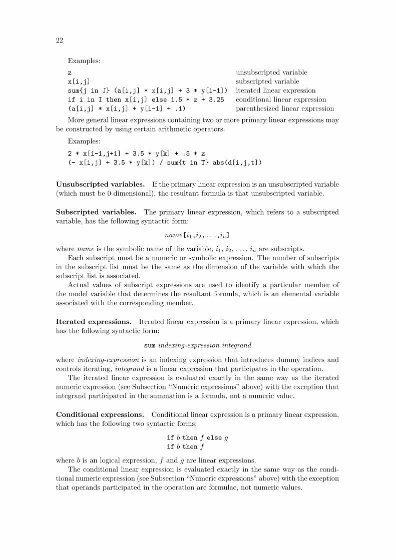
Examples:

z unsubscripted variablex[i,j] subscripted variablesum{j in J} (a[i,j] * x[i,j] + 3 * y[i-1]) iterated linear expressionif i in I then x[i,j] else 1.5 * z + 3.25 conditional linear expression(a[i,j] * x[i,j] + y[i-1] + .1) parenthesized linear expression

More general linear expressions containing two or more primary linear expressions maybe constructed by using certain arithmetic operators.

Examples:

2 * x[i-1,j+1] + 3.5 * y[k] + .5 * z(- x[i,j] + 3.5 * y[k]) / sum{t in T} abs(d[i,j,t])

Unsubscripted variables. If the primary linear expression is an unsubscripted variable(which must be 0-dimensional), the resultant formula is that unsubscripted variable.

Subscripted variables. The primary linear expression, which refers to a subscriptedvariable, has the following syntactic form:

name[i1,i2, . . . ,in]

where name is the symbolic name of the variable, i1, i2, . . . , in are subscripts.Each subscript must be a numeric or symbolic expression. The number of subscripts

in the subscript list must be the same as the dimension of the variable with which thesubscript list is associated.

Actual values of subscript expressions are used to identify a particular member ofthe model variable that determines the resultant formula, which is an elemental variableassociated with the corresponding member.

Iterated expressions. Iterated linear expression is a primary linear expression, whichhas the following syntactic form:

sum indexing-expression integrand

where indexing-expression is an indexing expression that introduces dummy indices andcontrols iterating, integrand is a linear expression that participates in the operation.

The iterated linear expression is evaluated exactly in the same way as the iteratednumeric expression (see Subsection “Numeric expressions” above) with the exception thatintegrand participated in the summation is a formula, not a numeric value.

Conditional expressions. Conditional linear expression is a primary linear expression,which has the following two syntactic forms:

if b then f else gif b then f

where b is an logical expression, f and g are linear expressions.The conditional linear expression is evaluated exactly in the same way as the condi-

tional numeric expression (see Subsection “Numeric expressions” above) with the exceptionthat operands participated in the operation are formulae, not numeric values.

23

Parenthesized expressions. Any linear expression may be enclosed in parenthesesthat syntactically makes it primary linear expression.

Parentheses may be used in linear expressions, as in algebra, to specify the desiredorder in which operations are to be performed. Where parentheses are used, the expressionwithin the parentheses is evaluated before the resultant formula is used.

The resultant value of the parenthesized expression is the same as the value of theexpression enclosed within parentheses.

Arithmetic operators. In MathProg there are the following arithmetic operators,which may be used in linear expressions:

+ f unary plus- f unary minusf + g additionf - g subtractionx * f , f * x multiplicationf / x division

where f and g are linear expressions, x is numeric expression.If the expression includes more than one arithmetic operator, all operators are per-

formed from left to right according to the hierarchy of operations (see below).The resultant value of the expression, which contains arithmetic operators, is the result

of applying the operators to their operands.

Hierarchy of operations. The hierarchy of arithmetic operations used in linear ex-pressions is the same as for numeric expressions (for details see Subsection “Numericexpressions”).

24

4 Statements

Statements are basic units of the model description. In MathProg all statements aredivided into two categories: declaration statements and functional statements.

Declaration statements (set statement, parameter statement, variable statement, con-straint statement, and objective statement) are used to declare model objects of certainkinds and define certain properties of that objects.

Functional statements (check statement and display statement) are basically intendedfor auxiliary purposes. The check statement allows checking correctness of data. Thedisplay statement allows displaying content of model objects that is usually needed ondebugging the model description.

MathProg is a descriptive, not procedural language. Therefore statements in the modeldescription may follow in arbitrary order which doesn’t affect the result of translation.However, any model object must be declared before it is referenced in other statements.

4.1 Set statement

General Form

set name alias domain , attrib , . . . , attrib ;

Where: name is the symbolic name of a set.alias is an optional string literal that specifies the alias of the set.domain is an optional indexing expression that specifies the subscriptdomain of the set.attrib, . . . , attrib are optional attributes of the set. (Commae precedingattributes may be omitted.)

The attributes are:dimen n specifies dimension of n-tuples, which the set consists of.within expression

specifies a superset which restricts the set or all its members (elementalsets) to be within this superset.

:= expression specifies an elemental set assigned to the set or its members.default expression

specifies an elemental set assigned to the set or its members wheneverno appropriate data are available in the data section.

Examples:

set nodes;set arcs within nodes cross nodes;set step{s in 1..maxiter} dimen 2 := if s = 1 then arcs else step[s-1]

union setof{k in nodes, (i,k) in step[s-1], (k,j) in step[s-1]}(i,j);set A{i in I, j in J}, within B[i+1] cross C[j-1], within D diff E,

default {(’abc’,123), (321,’cba’)};

The set statement declares a set. If the subscript domain is not specified, the set is asimple set, otherwise it is an array of elemental sets.

25

The dimen attribute specifies dimension of n-tuples, which the set (if it is a simpleset) or its members (if the set is an array of elemental sets) consist of, where n mustbe unsigned integer from 1 to 20. At most one dimen attribute can be specified. Ifthe dimen attribute is not specified, dimension of n-tuples is implicitly determined byother attributes (for example, if there is a set expression that follows := or the keyworddefault, the dimension of n-tuples of the corresponding elemental set is used). If nodimension information is available, dimen 1 is assumed.

The within attribute specifies a set expression whose resultant value is a superset usedto restrict the set (if it is a simple set) or its members (if the set is an array of elementalsets) to be within this superset. Arbitrary number of within attributes may be specifiedin the same set statement.

The assign (:=) attribute specifies a set expression used to evaluate elemental set(s)assigned to the set (if it is a simple set) or its members (if the set is an array of elementalsets). If the assign attribute is specified, the set is computable and therefore needs no datato be provided in the data section. If the assign attribute is not specified, the set must beprovided with data in the data section. At most one assign or default attribute can bespecified for the same set.

The default attribute specifies a set expression used to evaluate elemental set(s)assigned to the set (if it is a simple set) or its members (if the set is an array of elementalsets) whenever no appropriate data are available in the data section. If neither assign nordefault attribute is specified, missing data will cause an error.

4.2 Parameter statement

General Form

param name alias domain , attrib , . . . , attrib ;

Where: name is the symbolic name of a parameter.alias is an optional string literal that specifies the alias of the parameter.domain is an optional indexing expression that specifies the subscriptdomain of the parameter.attrib, . . . , attrib are optional attributes of the parameter. (Commaepreceding attributes may be omitted.)

The attributes are:integer specifies that the parameter is integer.binary specifies that the parameter is binary.symbolic specifies that the parameter is symbolic.relation expression (where relation is one of: < <= = == >= > <> !=)

specifies a condition that restricts the parameter or its members tosatisfy this condition.

in expression specifies a superset that restricts the parameter or its members to bein this superset.

:= expression specifies a value assigned to the parameter or its members.default expression

specifies a value assigned to the parameter or its members wheneverno appropriate data are available in the data section.

26

Examples:

param units{raw, prd} >= 0;param profit{prd, 1..T+1};param N := 20 integer >= 0 <= 100;param comb ’n choose k’ {n in 0..N, k in 0..n} :=

if k = 0 or k = n then 1 else comb[n-1,k-1] + comb[n-1,k];param p{i in I, j in J}, integer, >= 0, <= i+j, in A[i] symdiff B[j],

in C[i,j], default 0.5 * (i + j);param month symbolic default ’May’ in {’Mar’, ’Apr’, ’May’};

The parameter statement declares a parameter. If the subscript domain is not speci-fied, the parameter is a simple (scalar) parameter, otherwise it is a n-dimensional array.

The type attributes integer, binary, and symbolic qualify the type values which canbe assigned to the parameter as shown below:

Type attribute Assigned valuesnot specified Any numeric valuesinteger Only integer numeric valuesbinary Either 0 or 1symbolic Any numeric and symbolic values

The symbolic attribute cannot be specified along with other type attributes. Being spec-ified it must precede all other attributes.

The condition attribute specifies an optional condition that restricts values assigned tothe parameter to satisfy this condition. This attribute has the following syntactic forms:

< v Check for x < v<= v Check for x ≤ v= v, == v Check for x = v>= v Check for x ≥ v> v Check for x > v<> v, != v Check for x 6= v

where x is a value assigned to the parameter, v is the resultant value of a numeric orsymbolic expression specified in the condition attribute. If the parameter is symbolic,conditions in the form of inequality cannot be specified. Arbitrary number of conditionattributes can be specified for the same parameter. If a value being assigned to theparameter during model evaluation violates at least one specified condition, an error israised.

The in attribute is similar to the condition attribute and specifies a set expressionwhose resultant value is a superset used to restrict numeric or symbolic values assignedto the parameter to be in this superset. Arbitrary number of the in attributes can bespecified for the same parameter. If a value being assigned to the parameter during modelevaluation is not in at least one specified superset, an error is raised.

The assign (:=) attribute specifies a numeric or symbolic expression used to computea value assigned to the parameter (if it is a simple parameter) or its member (if theparameter is an array). If the assign attribute is specified, the parameter is computableand therefore needs no data to be provided in the data section. If the assign attribute is

27

not specified, the parameter must be provided with data in the data section. At most oneassign or default attribute can be specified for the same parameter.

The default attribute specifies a numeric or symbolic expression used to compute avalue assigned to the parameter or its member whenever no appropriate data are availablein the data section. If neither assign nor default attribute is specified, missing data willcause an error.

4.3 Variable statement

General Form

var name alias domain , attrib , . . . , attrib ;

Where: name is the symbolic name of a variable.alias is an optional string literal that specifies the alias of the variable.domain is an optional indexing expression that specifies the subscriptdomain of the variable.attrib, . . . , attrib are optional attributes of the variable. (Commaepreceding attributes may be omitted.)

The attributes are:integer restricts the variable to be integer.binary restricts the variable to be binary.>= expression specifies a lower bound of the variable.<= expression specifies an upper bound of the variable.= expression, == expression

specifies a fixed value of the variable.

Examples:

var x >= 0;var y{I,J};var make{p in prd}, integer, >= commit[p], <= market[p];var store{raw, 1..T+1} >= 0;var z{i in I, j in J} >= i+j;

The variable statement declares a variable. If the subscript domain is not specified,the variable is a simple (scalar) variable, otherwise it is a n-dimensional array of elementalvariables.

Elemental variable(s) associated with the model variable (if it is a simple variable) orits members (if it is an array) correspond to structural variables in the LP/MIP problemformulation (see Subsection “Linear programming problem”). Should note that only theelemental variables actually referenced in some constraints and objectives are included inthe LP/MIP problem instance to be generated.

The type attributes integer and binary restrict the variable to be integer or binary,respectively. If no type attribute is specified, the variable is continuous. If all variables inthe model are continuous, the corresponding problem is of LP class. If there is at leastone integer or binary variable, the problem is of MIP class.

The lower bound (>=) attribute specifies a numeric expression for computing the lowerbound of the variable. At most one lower bound can be specified. By default variables

28

(except binary ones) have no lower bounds, so if a variable is required to be non-negative,its zero lower bound should be explicitly specified.

The upper bound (<=) attribute specifies a numeric expression for computing the upperbound of the variable. At most one upper bound attribute can be specified.

The fixed value (=) attribute specifies a numeric expression for computing the value,at which the variable is fixed. This attribute cannot be specified along with lower/upperbound attributes.

4.4 Constraint statement

General Form

subject to name alias domain : expression , = expression ;

subject to name alias domain : expression , <= expression ;

subject to name alias domain : expression , >= expression ;

subject to name alias domain : expression , <= expression , <= expression ;

subject to name alias domain : expression , >= expression , >= expression ;

Where: name is the symbolic name of a constraint.alias is an optional string literal that specifies the alias of the constraint.domain is an optional indexing expression that specifies the subscriptdomain of the constraint.expressions are linear expressions for computing components of theconstraint. (Commae following expressions may be omitted.)

Note: The keyword subject to may be reduced to s.t. or omitted at all.

Examples:

s.t. r: x + y + z, >= 0, <= 1;limit{t in 1..T}: sum{j in prd} make[j,t] <= max_prd;subject to balance{i in raw, t in 1..T}:

store[i,t+1] - store[i,t] - sum{j in prd} units[i,j] * make[j,t];subject to rlim ’regular-time limit’ {t in time}:

sum{p in prd} pt[p] * rprd[p,t] <= 1.3 * dpp[t] * crews[t];

The constraint statement declares a constraint. If the subscript domain is not specified,the constraint is a simple (scalar) constraint, otherwise it is a n-dimensional array ofelemental constraints.

Elemental constraint(s) associated with the model constraint (if it is a simple con-straint) or its members (if it is an array) correspond to general linear constraints in theLP/MIP problem formulation (see Subsection “Linear programming problem”).

If the constraint has the form of equality or single inequality, i.e. includes two ex-pressions, one of which follows the colon and other follows the relation sign =, <=, or >=,both expressions in the statement can be linear expressions. If the constraint has the form

29

of double inequality, i.e. includes three expressions, the middle expression can be linearexpression while the leftmost and rightmost ones can be only numeric expressions.

Generating the model is, generally speaking, generating its constraints, which arealways evaluated for the entire subscript domain. Evaluating constraints leads, in turn,to evaluating other model objects such as sets, parameters, and variables.

Constructing the actual linear constraint included in the problem instantce, which(constraint) corresponds to a particular elemental constraint, is performed as follows.

If the constraint has the form of equality or single inequality, evaluation of both linearexpressions gives two resultant linear forms:

f = a1xm+1 + a2xm+2 + . . . + anxm+n + a0,g = b1xm+1 + b2xm+2 + . . . + bnxm+n + b0,

where xm+1, xm+2, . . . , xm+n are elemental variables, a1, a2, . . . , an, b1, b2, . . . , bn are nu-meric coefficients, a0 and b0 are constant terms. Then all linear terms of f and g arecarried to the left-hand side, and the constant terms are carried to the right-hand sidethat gives the final elemental constraint in the standard form:

xi : (a1 − b1)xm+1 + (a2 − b2)xm+2 + . . . + (an − bn)xm+n

=≤≥

b0 − a0,

where xi is the implicit auxiliary variable of the constraint (see Subsection “Linear pro-gramming problem”).

If the constraint has the form of double inequality, evaluation of the middle linearexpression gives the resultant linear form:

f = a1xm+1 + a2xm+2 + . . . + anxm+n + a0,

and evaluation of the leftmost and rightmost numeric expressions gives two numeric valuesl and u (or u and l), respectively. Then the constant term of the linear form is carriedto both left-hand and right-hand sides that gives the final elemental constraint in thestandard form:

l − a0 ≤ xi : a1xm+1 + a2xm+2 + . . . + anxm+n ≤ u− a0,

where xi is the implicit auxiliary variable of the constraint.

4.5 Objective statement

General Form

minimize name alias domain : expression ;

maximize name alias domain : expression ;

Where: name is the symbolic name of an objective.alias is an optional string literal that specifies the alias of the objective.domain is an optional indexing expression that specifies the subscriptdomain of the objective.expression is an linear expression that specifies the linear form of theobjective.

30

Examples:

minimize obj: x + 1.5 * (y + z);maximize total_profit: sum{p in prd} profit[p] * make[p];

The objective statement declares an objective. If the subscript domain is not specified,the objective is a simple (scalar) objective. Otherwise it is a n-dimensional array ofelemental objectives.

Elemental objective(s) associated with the model objective (if it is a simple objective)or its members (if it is an array) correspond to general linear constraints in the LP/MIPproblem formulation (see Subsection “Linear programming problem”). However, unlikeconstraints the corresponding linear forms are free (unbounded).

Constructing the actual linear constraint included in the problem instance, which(constraint) corresponds to a particular elemental objective, is performed as follows. Thelinear expression specified in the objective statement is evaluated that gives the resultantlinear form:

f = a1xm+1 + a2xm+2 + . . . + anxm+n + a0,

where xm+1, xm+2, . . . , xm+n are elemental variables, a1, a2, . . . , an are numeric coeffi-cients, a0 is the constant term. Then the linear form is used to construct the final elementalconstraint in the standard form:

−∞ ≤ xi : a1xm+1 + a2xm+2 + . . . + anxm+n + a0 ≤ +∞,

where xi is the implicit free (unbounded) auxiliary variable of the constraint.As a rule the model description contains only one objective statement that defines

the objective function (1) used in the problem instance. However, it is allowed to declarearbitrary number of objectives, in which case the actual objective function is the firstobjective encountered in the model description. Other objectives are also included in theproblem instance, but they don’t affect the objective function.

4.6 Check statement

General Form

check domain : expression ;

Where: domain is an optional indexing expression that specifies the subscriptdomain of the check statement.expression is an logical expression that specifies the logical conditionto be checked. (The colon preceding expression may be omitted.)

Examples:

check: x + y <= 1 and x >= 0 and y >= 0;check sum{i in ORIG} supply[i] = sum{j in DEST} demand[j];check{i in I, j in 1..10}: S[i,j] in U[i] union V[j];

The check statement allows checking the resultant value of an logical expression spec-ified in the statement. If the value is false, the model translator reports an error.

31

If the subscript domain is not specified, the check is performed only once. Specifyingthe subscript domain allows performing multiple checks for every n-tuple in the domainset. In the latter case the logical expression may include dummy indices introduced in theindexing expression that specifies the subscript domain.

4.7 Display statement

General Form

display domain : item , . . . , item ;

Where: domain is an optional indexing expression that specifies the subscriptdomain of the display statement.item , . . . , item are items to be displayed. (The colon preceding thefirst item may be omitted.)

Examples:

display: ’x =’, x, ’y =’, y, ’z =’, z;display sqrt(x ** 2 + y ** 2 + z ** 2);display{i in I, j in J}: i, j, a[i,j], b[i,j];

The display statement evaluates all items specified in the statement and writes theirvalues on the standard output in plain text format.

If the subscript domain is not specified, items are evaluated and then displayed onlyonce. Specifying the subscript domain causes evaluating and displaying items for everyn-tuple in the domain set. In the latter case items may include dummy indices introducedin the indexing expression that specifies the subscript domain.

Item to be displayed can be a model object (set, parameter, variable, constraint,objective) or an expression.

If the item is a computable object (i.e. a set or parameter provided with the assignattribute), the object is evaluated over the entire domain and then its content (i.e. thecontent of the object array) is displayed. Otherwise, if the item is not a computableobject, only its current content (i.e. the members actually generated during the modelevaluation) is displayed. Note that if the item is a variable, its “value” displayed bythe display statement means “elemental variable”, not a numeric value, which the variablecould have in some solution obtained by the solver. Analogously, if the item is a constraintor objective, its “value” means “elemental constraint” or “elemental objective”.

If the item is an expression, the expression is evaluated and its resultant value isdisplayed.

32

5 Model data

Model data include elemental sets, which are “values” of model sets, and numeric andsymbolic values of model parameters.

In MathProg there are two different ways to saturate model sets and parameters withdata. One way is simply providing necessary data using the assign attribute. However,in many cases it is more practical to separate the model itself and particular data neededfor the model. For the latter reason in MathProg there is other way, when the modeldescription is divided into two parts: model section and data section.

Model section is a main part of the model description that contains declarations of allmodel objects and is common for all problems based on that model.

Data section is an optional part of the model description that contains model dataspecific for a particular problem.

In MathProg model and data sections can be placed either in one text file or in twoseparate text files.

If both model and data sections are placed in one file, the file is composed as follows:

statementstatement. . .statementdata;data blockdata block. . .data blockend;

If the model and data sections are placed in two separate files, the files are composedas follows:

statementstatement. . .statementend;

data;data blockdata block. . .data blockend;

Model file Data file

Note: If the data section is placed in a separate file, the keyword data is optional andmay be omitted along with the semicolon that follows it.

5.1 Coding data section

The data section is a sequence of data blocks in various formats, which are discussed infollowing subsections. The order, in which data blocks follow in the data section, may bearbitrary, not necessarily the same as in which the corresponding model objects follow inthe model section.

The rules of coding the data section are commonly the same as the rules of coding themodel description (for details see Section “Coding model description”), i.e. data blocks

33

are composed from basic lexical units such as symbolic names, numeric and string literals,keywords, delimiters, and comments. However, for the sake of convenience and improvingreadability there is one deviation from the common rule: if a string literal consists of onlyalphanumeric characters (including the underscore character), the signs + and -, and/orthe decimal point, it may be coded without bordering (single or double) quotes.

All numeric and symbolic material provided in the data section is coded in the formof numbers and symbols, i.e. unlike the model section no expressions are allowed in thedata section. Nevertheless the signs + and - can precede numeric literals to allow codingsigned numeric quantities, in which case there must be no white-space characters betweenthe sign and following numeric literal (if there is at least one white-space, the sign andfollowing numeric literal are recognized as two different lexical units).

5.2 Set data block

General Form

set name , record , . . . , record ;

set name [ symbol , . . . , symbol ] , record , . . . , record ;

Where: name is the symbolic name of a set.symbol, . . . , symbol are subscripts that specify a particular member ofthe set (if the set is an array, i.e. set of sets).record, . . . , record are data records.

Note: Commae preceding data records may be omitted.

The data records are::= is a non-significant data record which may be used freely to improve

readability.( slice ) specifies a slice.simple-data specifies set data in the simple format.: matrix-data specifies set data in the matrix format.(tr) : matrix-data

specifies set data in the transposed matrix format. (In this case thecolon following the keyword (tr) may be omitted.)

Examples:

set month := Jan Feb Mar Apr May Jun;set month "Jan", "Feb", "Mar", "Apr", "May", "Jun";set A[3,Mar] := (1,2) (2,3) (4,2) (3,1) (2,2) (4,4) (3,4);set A[3,’Mar’] := 1 2 2 3 4 2 3 1 2 2 4 4 2 4;set A[3,’Mar’] : 1 2 3 4 :=

1 - + - -2 - + + -3 + - - +4 - + - + ;

34

set B := (1,2,3) (1,3,2) (2,3,1) (2,1,3) (1,2,2) (1,1,1) (2,1,1);set B := (*,*,*) 1 2 3, 1 3 2, 2 3 1, 2 1 3, 1 2 2, 1 1 1, 2 1 1;set B := (1,*,2) 3 2 (2,*,1) 3 1 (1,2,3) (2,1,3) (1,1,1);set B := (1,*,*) : 1 2 3 :=

1 + - -2 - + +3 - + -

(2,*,*) : 1 2 3 :=1 + - +2 - - -3 + - - ;

(In these examples the set month is a simple set of singles, A is a 2-dimensional array ofdoubles, and B is a simple set of triples. Data blocks for the same set are equivalent in thesense that they specify the same data in different formats.)

The set data block is used to specify a complete elemental set, which is assigned to aset (if it is a simple set) or one of its members (if the set is an array of sets).2

Data blocks can be specified only for the sets, which are non-computable, i.e. whichhave no assign attribute in the corresponding set statements.

If the set is a simple set, only its symbolic name should be given in the header of thedata block. Otherwise, if the set is a n-dimensional array, its symbolic name should beprovided with a complete list of subscripts separated by commae and enclosed in squarebrackets to specify a particular member of the set array. The number of subscripts mustbe the same as the dimension of the set array, where each subscript must be a number orsymbol.

The elemental set defined in the set data block is coded as a sequence of data recordsdescribed below.3

Assign data record. The assign (:=) data record is a non-signficant element. It maybe used for improving readability of data blocks.

Slice data record. The slice data record is a control record that specifies a slice of theelemental set defined in the data block. It has the following syntactic form:

(s1,s2, . . . ,sn)

where s1, s2, . . . , sn are components of the slice.Each component of the slice can be a number or symbol or the asterisk (*). The number

of components in the slice must be the same as the dimension of n-tuples in the elementalset to be defined. For instance, if the elemental set contains 4-tuples (quadruples), the slicemust have four components. The number of asterisks in the slice is called slice dimension.

The effect of using slices is the following. If a m-dimensional slice (i.e. a slice thathas m asterisks) is specified in the data block, all subsequent data records must specifiytuples of the dimension m. Whenever a m-tuple is encountered, each asterisk in the slice

2There is another way to specify data for a simple set along with data for parameters. This feature isdiscussed in the next subsection.

3Data record is simply a technical term. It does not mean that data records have any special formatting.

35

is replaced by corresponding components of the m-tuple that gives the resultant n-tuple,which is included in the elemental set to be defined. For example, if the slice (a, ∗, 1, 2, ∗)is in effect, and the 2-tuple (3, b) is encountered in a subsequent data record, the resultant5-tuple included in the elemental set is (a, 3, 1, 2, b).

The slice that has no asterisks itself defines a complete n-tuple, which is included inthe elemental set.

Being once specified the slice effects until either a new slice or the end of data blockhas been encountered. Note that if there is no slice specified in the data block, a dummyone, components of which are all asterisks, is assumed.

Simple data record. The simple data record defines one n-tuple in simple format andhas the following syntactic form:

t1,t2, . . . ,tn

where t1, t2, . . . , tn are components of the n-tuple. Each component can be a number orsymbol. Commae between components are optional and may be omitted.

Matrix data record. The matrix data record defines several 2-tuples (doubles) in ma-trix format and has the following syntactic form:

: c1 c2 . . . cn :=r1 a11 a12 . . . a1n

r2 a21 a22 . . . a2n

. . . . . . . . . . . . . . .rm am1 am2 . . . amn

where r1, r2, . . . , rm are numbers and/or symbols that correspond to rows of the ma-trix, c1, c2, . . . , cn are numbers and/or symbols that correspond to columns of the matrix,a11, a12, . . . , amn are the matrix elements, which can be the signs + and -. (In this datarecord the delimiter : that precedes the column list and the delimiter := that follows thecolumn list cannot be omitted.)

Each element aij of the matrix data block (where 1 ≤ i ≤ m, 1 ≤ j ≤ n) correspondsto the 2-tuple (ri, cj). If aij is the plus (+) sign, the corresponding 2-tuple (or longern-tuple, if a slice is used) is included in the elemental set. Otherwise, if aij is the minus(-) sign, the corresponding 2-tuple is not included in the elemental set.

Since the matrix data record defines 2-tuples, either the elemental set must consist of2-tuples or the slice currently used must be 2-dimensional.

Transposed matrix data record. The transposed matrix data record has the followingsyntactic form:

(tr) : c1 c2 . . . cn :=r1 a11 a12 . . . a1n

r2 a21 a22 . . . a2n

. . . . . . . . . . . . . . .rm am1 am2 . . . amn

(In this case the delimiter : that follows the keyword (tr) is optional and may be omitted.)This data record is completely analogous to the matrix data record (see above) with

the only exception that each element aij of the matrix corresponds to the 2-tuple (cj , ri).Being once specified the (tr) indicator effects on all subsequent data records until

either a slice or the end of data block has been encountered.

36

5.3 Parameter data block

General Form

param name , record , . . . , record ;

param name default value , record , . . . , record ;

param : tabbing-data ;

param default value : tabbing-data ;

Where: name is the symbolic name of a parameter.value is an optional default value of the parameter.record, . . . , record are data records.tabbing-data specifies parameter data in the tabbing format.

Note: Commae preceding data records may be omitted.

The data records are::= is a non-significant data record which may be used freely to improve

readability.[ slice ] specifies a slice.plain-data specifies parameter data in the plain format.: tabular-data specifies parameter data in the tabular format.(tr) : tabular-data

specifies parameter data in the transposed tabular format. (In this casethe colon following the keyword (tr) may be omitted.)

Examples:

param T := 4;param month := 1 Jan 2 Feb 3 Mar 4 Apr 5 May;param month := [1] ’Jan’, [2] ’Feb’, [3] ’Mar’, [4] ’Apr’, [5] ’May’;param init_stock := iron 7.32 nickel 35.8;param init_stock [*] iron 7.32, nickel 35.8;param cost [iron] .025 [nickel] .03;param value := iron -.1, nickel .02;param : init_stock cost value :=

iron 7.32 .025 -.1nickel 35.8 .03 .02 ;

param : raw : init stock cost value :=iron 7.32 .025 -.1nickel 35.8 .03 .02 ;

param demand default 0 (tr): FRA DET LAN WIN STL FRE LAF :=

bands 300 . 100 75 . 225 250coils 500 750 400 250 . 850 500plate 100 . . 50 200 . 250 ;

37

param trans_cost :=[*,*,bands]: FRA DET LAN WIN STL FRE LAF :=

GARY 30 10 8 10 11 71 6CLEV 22 7 10 7 21 82 13PITT 19 11 12 10 25 83 15

[*,*,coils]: FRA DET LAN WIN STL FRE LAF :=GARY 39 14 11 14 16 82 8CLEV 27 9 12 9 26 95 17PITT 24 14 17 13 28 99 20

[*,*,plate]: FRA DET LAN WIN STL FRE LAF :=GARY 41 15 12 16 17 86 8CLEV 29 9 13 9 28 99 18PITT 26 14 17 13 31 104 20 ;

The parameter data block is used to specify complete data for a parameter (or param-eters, if data are specified in the tabbing format) whose name is given in the block.

Data blocks can be specified only for the parameters, which are non-computable, i.e.which have no assign attribute in the corresponding parameter statements.

Data defined in the parameter data block are coded as a sequence of data recordsdescribed below. Additionally the data block can be provided with the optional defaultattribute, which specifies a default numeric or symbolic value of the parameter (parame-ters). This default value is assigned to the parameter or its members, if no appropriatevalue is defined in the parameter data block. The default attribute cannot be used, if itis already specified in the corresponding parameter statement(s).

Assign data record. The assign (:=) data record is a non-signficant element. It maybe used for improving readability of data blocks.

Slice data record. The slice data record is a control record that specifies a slice of theparameter array. It has the following syntactic form:

(s1,s2, . . . ,sn)

where s1, s2, . . . , sn are components of the slice.Each component of the slice can be a number or symbol or the asterisk (*). The number

of components in the slice must be the same as the dimension of the parameter. Forinstance, if the parameter is a 4-dimensional array, the slice must have four components.The number of asterisks in the slice is called slice dimension.

The effect of using slices is the following. If a m-dimensional slice (i.e. a slice that has masterisks) is specified in the data block, all subsequent data records must specify subscriptsof the parameter members as if the parameter were m-dimensional, not n-dimensional.

Whenever m subscripts are encountered, each asterisk in the slice is replaced by cor-responding subscript that gives n subscripts, which define the actual parameter member.For example, if the slice [a, ∗, 1, 2, ∗] is in effect, and the subscripts 3 and b are encoun-tered in a subsequent data record, the complete subscript list used to choose a parametermember is [a, 3, 1, 2, b].

It is allowed to specify a slice that has no asterisks. Such slice itself defines a completesubscript list, in which case the next data record can define only a single value of thecorresponding parameter member.

38

Being once specified the slice effects until either a new slice or the end of data blockhas been encountered. Note that if there is no slice specified in the data block, a dummyone, components of which are all asterisks, is assumed.

Plain data record. The plain data record defines the subscript list and a single valuein plain format. This record has the following syntactic form:

t1,t2, . . . ,tn,v

where t1, t2, . . . , tn are subscripts, v is a value. Each subscript as well as the value can bea number or symbol. Commae that follow subscripts are optional and may be omitted.

In case of 0-dimensional parameter or slice the plain data record have no subscriptsand consists of a single value only.

Tabular data record. The tabular data record defines several values, where each valueis provided with two subscripts. This record has the following syntactic form:

: c1 c2 . . . cn :=r1 a11 a12 . . . a1n

r2 a21 a22 . . . a2n

. . . . . . . . . . . . . . .rm am1 am2 . . . amn

where r1, r2, . . . , rm are numbers and/or symbols that correspond to rows of the ma-trix, c1, c2, . . . , cn are numbers and/or symbols that correspond to columns of the table,a11, a12, . . . , amn are the table elements. Each element can be a number or symbol or thesingle decimal point. (In this data record the delimiter : that precedes the column listand the delimiter := that follows the column list cannot be omitted.)

Each element aij of the tabular data block (1 ≤ i ≤ m, 1 ≤ j ≤ n) defines twosubscripts, where the first subscript is ri, and the second one is cj . These subscripts areused in conjunction with the current slice to form the complete subscript list that identifiesa particular member of the parameter array. If aij is a number or symbol, this value isassigned to the parameter member. However, if aij is the single decimal point, the memberis assigned a default value specified either in the parameter data block or in the parameterstatement, or, if no default value is specified, the member remains undefined.

Since the tabular data record provides two subscripts for each value, either the pa-rameter or the slice currently used must be 2-dimensional.

Transposed tabular data record. The transposed tabular data record has the follow-ing syntactic form:

(tr) : c1 c2 . . . cn :=r1 a11 a12 . . . a1n

r2 a21 a22 . . . a2n

. . . . . . . . . . . . . . .rm am1 am2 . . . amn

(In this case the delimiter : that follows the keyword (tr) is optional and may be omitted.)This data record is completely analogous to the tabular data record (see above) with

the only exception that the first subscript defined by the element aij is cj while the secondone is ri.

39

Being once specified the (tr) indicator effects on all subsequent data records untileither a slice or the end of data block has been encountered.

Tabbing data format. The parameter data block in the tabbing format has the fol-lowing syntactic form:

param default value : s : p1 , p2 , . . . , pr :=r11 , r12 , . . . , r1n , a11 , a12 , . . . , a1r ,r21 , r22 , . . . , r2n , a21 , a22 , . . . , a2r ,. . . . . . . . . . . . . . . . . . . . . . . .rm1 , rm2 , . . . , rmn , am1 , am2 , . . . , amr ;

Notes:1. The keyword default may be omitted along with a value that follows it.2. The symbolic name s of a set may be omitted along with the colon that follows it.3. All comae are optional and may be omitted.The data block in the tabbing format shown above is exactly equivalent to the following

data blocks:

set s := (r11,r12, . . . ,r1n) (r21,r22, . . . ,r2n) . . . (rm1,rm2, . . . ,rmn);param p1 default value :=

[r11,r12, . . . ,r1n] a11 [r21,r22, . . . ,r2n] a21 . . . [rm1,rm2, . . . ,rmn] am1;param p2 default value :=

[r11,r12, . . . ,r1n] a12 [r21,r22, . . . ,r2n] a22 . . . [rm1,rm2, . . . ,rmn] am2;. . . . . . . . .

param pr default value :=[r11,r12, . . . ,r1n] a1r [r21,r22, . . . ,r2n] a2r . . . [rm1,rm2, . . . ,rmn] amr;

40

A Using the MathProg translator with GLPK API

The GLPK package includes the API routine lpx_read_model, which is a high-level in-terface to the GNU MathProg translator.

Synopsis

#include "glpk.h"LPX *lpx_read_model(char *model, char *data, char *output);

Description The routine lpx_read_model reads and translates LP/MIP model (prob-lem) written in the GNU MathProg modeling language.

The character string model specifies name of input text file, which contains modelsection and, optionally, data section. This parameter cannot be NULL.

The character string data specifies name of input text file, which contains data section.This parameter can be NULL. (If the data file is specified and the model file also containsdata section, that section is ignored and data section from the data file is used.)

The character string output specifies name of output text file, to which the outputproduced by display statements is written. If the parameter output is NULL, the displayoutput is sent to stdout via the routine print.

Returns If no errors occurred, the routine returns a pointer to the created problemobject. Otherwise the routine sends diagnostics to the standard output and returns NULL.

41

B Solving models with the solver glpsol

The GLPK package includes the program glpsol which is a stand-alone LP/MIP solver.This program can be invoked from the command line or from the shell to solve modelswritten in the GNU MathProg modeling language.

In order to tell the solver that the input file contains a model description, the option--model should be specified in the command line. For example:

glpsol --model foobar.mod

Sometimes it is necessary to use the data section placed in another file, in which casethe following command may be used:

glpsol --model foobar.mod --data foobar.dat

Note that if the model file also contains the data section, that section is ignored.If the model description contains some display statements, by default the display

output goes onto the screen (more precisely, onto the standard output device). In orderto redirect the display output to a file the following command may be used:

glpsol --model foobar.mod --display foobar.out

If you need to look at the problem which has been generated by the model translator,the option --wtxt should be specified in the command line as follows:

glpsol --model foobar.mod --wtxt foobar.txt

in which case the problem will be written to the file foobar.txt in plain text formatsuitable for visual analysis.

Sometimes it is necessary merely to check the model description not solving the gen-erated problem. In this case the option --check should be given in the command line, forexample:

glpsol --check --model foobar.mod --wtxt foobar.txt

In order to write a numeric solution obtained by the solver the following commandmay be used

glpsol --model foobar.mod --output foobar.sol

in which case the solution will be written to the file foobar.sol in plain text format.Complete list of the glpsol options can be found in the reference manual included in

the GLPK distribution.

42

C Example of model description

C.1 Model description written in GNU MathProg

This is a complete example of model description written in the GNU MathProg modelinglanguage.

# A TRANSPORTATION PROBLEM## This problem finds a least cost shipping schedule that meets# requirements at markets and supplies at factories.## References:# Dantzig, G B., Linear Programming and Extensions# Princeton University Press, Princeton, New Jersey, 1963,# Chapter 3-3.

set I;/* canning plants */

set J;/* markets */

param a{i in I};/* capacity of plant i in cases */

param b{j in J};/* demand at market j in cases */

param d{i in I, j in J};/* distance in thousands of miles */

param f;/* freight in dollars per case per thousand miles */

param c{i in I, j in J} := f * d[i,j] / 1000;/* transport cost in thousands of dollars per case */

var x{i in I, j in J} >= 0;/* shipment quantities in cases */

minimize cost: sum{i in I, j in J} c[i,j] * x[i,j];/* total transportation costs in thousands of dollars */

s.t. supply{i in I}: sum{j in J} x[i,j] <= a[i];/* observe supply limit at plant i */

s.t. demand{j in J}: sum{i in I} x[i,j] >= b[j];/* satisfy demand at market j */

data;

set I := Seattle San-Diego;

set J := New-York Chicago Topeka;

43

param a := Seattle 350San-Diego 600;

param b := New-York 325Chicago 300Topeka 275;

param d : New-York Chicago Topeka :=Seattle 2.5 1.7 1.8San-Diego 2.5 1.8 1.4 ;

param f := 90;

end;

C.2 Generated LP problem

This is the LP problem that has been generated by the model translator for the examplemodel description.

Problem: TRANSPClass: LPRows: 6Columns: 6Non-zeros: 18

*** OBJECTIVE FUNCTION ***

Minimize: cost0.225 x[Seattle,New-York]0.153 x[Seattle,Chicago]0.162 x[Seattle,Topeka]0.225 x[San-Diego,New-York]0.162 x[San-Diego,Chicago]0.126 x[San-Diego,Topeka]

*** ROWS (CONSTRAINTS) ***

Row 1: cost free0.126 x[San-Diego,Topeka]0.225 x[San-Diego,New-York]0.153 x[Seattle,Chicago]0.225 x[Seattle,New-York]0.162 x[Seattle,Topeka]0.162 x[San-Diego,Chicago]

Row 2: supply[Seattle] <= 3501 x[Seattle,Chicago]1 x[Seattle,New-York]1 x[Seattle,Topeka]

Row 3: supply[San-Diego] <= 6001 x[San-Diego,Chicago]1 x[San-Diego,New-York]1 x[San-Diego,Topeka]

44

Row 4: demand[New-York] >= 3251 x[Seattle,New-York]1 x[San-Diego,New-York]

Row 5: demand[Chicago] >= 3001 x[Seattle,Chicago]1 x[San-Diego,Chicago]

Row 6: demand[Topeka] >= 2751 x[Seattle,Topeka]1 x[San-Diego,Topeka]

*** COLUMNS (VARIABLES) ***

Col 1: x[Seattle,New-York] >= 00.225 (objective)0.225 cost

1 supply[Seattle]1 demand[New-York]

Col 2: x[Seattle,Chicago] >= 00.153 (objective)0.153 cost

1 supply[Seattle]1 demand[Chicago]

Col 3: x[Seattle,Topeka] >= 00.162 (objective)0.162 cost

1 supply[Seattle]1 demand[Topeka]

Col 4: x[San-Diego,New-York] >= 00.225 (objective)0.225 cost

1 supply[San-Diego]1 demand[New-York]

Col 5: x[San-Diego,Chicago] >= 00.162 (objective)0.162 cost

1 supply[San-Diego]1 demand[Chicago]

Col 6: x[San-Diego,Topeka] >= 00.126 (objective)0.126 cost

1 supply[San-Diego]1 demand[Topeka]

End of output

45

C.3 Optimal solution of the generated LP problem

This is the optimal solution of the generated LP problem that has been found by theGLPK simplex solver.

Problem: TRANSPRows: 6Columns: 6Non-zeros: 18Status: OPTIMALObjective: cost = 153.675 (MINimum)

No. Row name St Activity Lower bound Upper bound Marginal------ ------------ -- ------------- ------------- ------------- -------------

1 cost B 153.6752 supply[Seattle]

B 300 3503 supply[San-Diego]

NU 600 600 < eps4 demand[New-York]

NL 325 325 0.2255 demand[Chicago]

NL 300 300 0.1536 demand[Topeka]

NL 275 275 0.126

No. Column name St Activity Lower bound Upper bound Marginal------ ------------ -- ------------- ------------- ------------- -------------

1 x[Seattle,New-York]B 0 0

2 x[Seattle,Chicago]B 300 0

3 x[Seattle,Topeka]NL 0 0 0.036

4 x[San-Diego,New-York]B 325 0

5 x[San-Diego,Chicago]NL 0 0 0.009

6 x[San-Diego,Topeka]B 275 0

End of output