modeling iriscode and its variants as convex polyhedral

1

Modeling IrisCode and its Variants as Convex Polyhedral Cones and its Security Implications

Adams Wai Kin Kong, IEEE Member

Forensics and Security Laboratory, School of Computer Engineering, Nanyang Technological University, Nanyang Avenue, Singapore, 639798 (Email: [email protected])

Abstract IrisCode, developed by Daugman in 1993, is the most influential iris recognition algorithm.

A thorough understanding of IrisCode is essential, because over 100 million persons have been enrolled

by this algorithm and many biometric personal identification and template protection methods have been

developed based on IrisCode. This paper indicates that a template produced by IrisCode or its variants is a

convex polyhedral cone in a hyperspace. Its central ray, being a rough representation of the original

biometric signal, can be computed by a simple algorithm, which can often be implemented in one

MATLAB command line. The central ray is an expected ray and also an optimal ray of an objective

function on a group of distributions. This algorithm is derived from geometric properties of a convex

polyhedral cone but does not rely on any prior knowledge (e.g., iris images). The experimental results

show that biometric templates, including iris and palmprint templates, produced by different recognition

methods can be matched through the central rays in their convex polyhedral cones and that templates

protected by a method extended from IrisCode can be broken into. These experimental results indicate

that, without a thorough security analysis, convex polyhedral cone templates cannot be assumed secure.

Additionally, the simplicity of the algorithm implies that even junior hackers without knowledge of

advanced image processing and biometric databases can still break into protected templates and reveal

relationships among templates produced by different recognition methods.

Keywords: Biometrics, iris recognition, template protection, palmprint recognition.

2

1. Introduction

IrisCode1 has over 100 million users from approximately 170 countries [1]. As of 4 January 2012, the total

number of people just in India who have had their iris patterns enrolled by IrisCode is 103 million. The Unique

Identification Authority of India is enrolling about one million persons per day, at 40,000 stations, and they

plan to have the entire population of 1.2 billion people enrolled within 3 years [33]. The extraordinary market

success of IrisCode relies heavily on its computational advantages, including extremely high matching speed

for large-scale identification and automatic threshold adjustment based on image quality (e.g., number of

effective bits) and database size [1-3]. In the last two decades, this algorithm influenced many researchers [4-

15]. Many methods modified from IrisCode were proposed for iris, palmprint, and finger-knuckle recognition.

This paper refers to these methods as generalized IrisCodes (GIrisCode) [4]. The simplest modification

replaced the Gabor filters in IrisCode with other linear filters or transforms. A more complex modification

used a clustering scheme to perform feature extraction and a special coding table to perform feature encoding

[4-5]. With these modifications, feature value precision could be increased, and many IrisCode computational

advantages could be retained. Another modification replaced the Gabor filters in IrisCode with random vectors

to construct cancelable biometrics for template protection [16-17]. A complete understanding of IrisCode is

thus necessary. Though many research papers regarding iris recognition have been published, our

understanding of this important algorithm remains incomplete. Daugman indicated that the imposter

distribution of IrisCode follows a binomial distribution, and the bits “0” and “1” in IrisCode are equally

probable [1]. Hollingsworth et al.2 analyzed bit stability in their iris codes and detected the best bits for

enhancing recognition performance [18]. Kong and his coworkers theoretically derived the following points:

IrisCode is a clustering algorithm with four prototypes and a compression algorithm; the Gabor function can be

regarded as a phase-steerable filter; the locus of a Gabor function is a two-dimensional ellipse with respect to a

phase parameter and can often be approximated by a circle; the bitwise hamming distance can be considered a

bitwise phase distance; and Gabor filters can be utilized as a Gabor atom detector, and the magnitude and

phase of a target Gabor atom can be approximated by the magnitude and phase of the corresponding Gabor

1 In this paper, IrisCode is used interchangeably to refer to both the method and features of iris recognition developed by Daugman. 2 Hollingsworth et al. used 1D log-Gabor wavelets instead of 2D Gabor filters in their study [18].

3

response [4, 19-20]. Using these theoretical results and information from iris image databases, Kong designed

an algorithm to reconstruct iris images from IrisCodes [20]. Nevertheless, the geometric structure of IrisCodes

has never been studied. This paper primarily aims to provide a deeper understanding of the geometric

structures of IrisCode and its variants and secondarily seeks to analyze the potential security and privacy risks

from this geometric information.

Though the IrisCode computational procedures are well-known, we present a brief computational

summary for notation consistency. Two-dimensional Gabor filters with zero DC are used to extract phase

information from an iris image in a dimensionless polar coordinate system, 0( , ) Ι . The complex Gabor

response is quantized into two bits by the following inequalities:

2 2 2 20 0 0( ) / ( ) / ( )

01 Re ( , ) 0j j j j j jr ijrb if e e e d d

I , (1)

2 2 2 20 0 0( ) / ( ) / ( )

00 Re ( , ) 0j j j j j jr ijrb if e e e d d

I , (2)

2 2 2 20 0 0( ) / ( ) / ( )

01 Im ( , ) 0j j j j j jr ijib if e e e d d

I , (3)

2 2 2 20 0 0( ) / ( ) / ( )

00 Im ( , ) 0j j j j j jr ijib if e e e d d

I , (4)

where j is the spatial frequency, j and j control the shape of the Gaussian function and 0 0( , )j jr is the

center/location of the filter in the spatial domain [2]. One thousand and twenty-four Gabor filters with

different parameters 0 0( , , , , )j j j j jr generate 1024 bit pairs ( , )jr jib b in an IrisCode, and a mask

excludes the corrupted bits from the eyelashes, eyelids, reflection, and a low signal-to-noise ratio [2].

Bitwise hamming distance is employed for high speed matching. Although Eqs. 1-4 are given as

integrations over a filter kernel, in the rest of this paper, two dimensional functions are expressed in

discrete form as matrices and that these matrices are expressed as vectors after lexicographic ordering.

Therefore, all filtering operations will be expressed as inner products.

4

The rest of this paper is organized as follows: Section 2 gives an introduction to convex polyhedral

cone, presents an algorithm to estimate its central ray and reveals the relationships among the central ray,

the expected ray and the optimal ray of an objective function on a group of distributions. Section 3 shows

that a template produced by IrisCode or GIrisCode is a convex polyhedral cone in a hyperspace. Section 4

reports the experimental results obtained from iris recognition methods, palmprint recognition methods,

and a security analysis of a template protection method. Section 5 discusses the impact of our theoretical

and experimental findings.

2. Estimating the Central Ray of a Convex Polyhedral Cone

For clear presentation, a set of notations is necessary. Given a zero DC Gabor filter jg with parameters

0 0( , , , , )j j j j jr , which generates a bit pair ( , )j jr jiB b b in an IrisCode, jrg and jig represent its

real and imaginary parts. I is used to denote 0 ( , ) Ι . 0Ι can be computed from I, because can never

be zero. For other biometric methods, I represents an original image and biometric signal. Bold font is

used to denote matrices and both two-dimensional filters and images. For example, jig is an imaginary

part of a two-dimensional Gabor filter, while jig is a column vector form of jig , and I is a two-

dimensional image, while I is a column vector form of the image. T represents the transpose of a matrix or

vector. Therefore, the inner product of two real valued vectors (e.g., jrg and krg ) can be defined as

, Tjr kr kr jrg g g g .

2.1. Fundamental Knowledge of a Convex Polyhedral Cone

Convex polytope, a branch of mathematics, has strong connections with constraint optimization (e.g.,

linear programming) [21-22]. A convex polyhedral cone is a special type of convex polytope. In this

subsection, we introduce the convex polyhedral cone for readers without background knowledge.

5

A convex polytope can be defined in several different ways. This paper uses the half-space

representation, which defines a convex polytope through the intersection of closed half-spaces. Let

dC be a convex polytope. Using the half-space representation, : dC x x z Q , where

m dQ and mz . Each row in the inequality system describes a half-space, i.e., k kq x z [21],

where kq is the kth row in Q, and zk is the kth element in z. Note that k kq x z is a hyperplane. When z is a

zero vector, C becomes a convex polyhedral cone with apex zero [22]. This paper considers only convex

polyhedral cones with apex zero; : 0dC x x Q is thus used as a definition of the convex

polyhedral cone. Three properties can be derived: (1) C is a convex set; (2) the intersection of convex

polyhedral cones is also a convex polyhedral cone; and (3) if x C , then x C , 0 , where x is

called a ray. The following discussion uses these three properties. Fig. 1 illustrates convex polyhedral

cones and other cones. Fig. 2 illustrates that the intersection of convex polyhedral cones is also a convex

polyhedral cone.

(a)

(b)

(c)

(d)

Fig. 1 Illustration of convex polyhedral cones and other cones. (a) and (b) convex polyhedral cones, (c) a non-convex polyhedral cone and (d) a circular cone.

6

Fig. 2 The intersection of convex polyhedral cones is also a convex polyhedral cone.

The half-space representation is not unique. In other words, there exists more than one inequality

system representing the same convex polyhedral cone. For example,

1 121

2 2

1 0: 0

0 1

x xC

x x

, (5)

and

1 122

2 2

1 0

: 0 1 0

1 1

x xC

x x

, (6)

represent the same convex polyhedral cone (Fig. 3), but their inequality systems differ. The inequality

1 2 0x x in Eq. 6 is a redundant constraint that can be removed. Note that the number of inequalities

in the minimal representation is unique [24]. Several ways exist to remove redundant constraints in a

linear inequality system. A simple one is based on linear programming. Let us consider an inequality

system q

zx

zq

Q, where m dQ , dx , mz , 1 dq , and qz . If qqx z is a redundant

constraint in the linear inequality system, then qz , where is defined as

max subject to1q

zqx x

zq

Q. (7)

7

Eq. 7 can be solved by linear programming. Convex hull algorithms can also remove redundant

constraints [23].

X1

X2

X1≥0 X1≥0

X2≥0

X2≥0

C1

(a)

(b)

Fig. 3 Illustration of a non-unique representation of a convex polyhedral cone and a redundant constraint. (a) the convex polyhedral cone C1 defined by Eq. 5 and (b) the convex polyhedral cone C2 defined by Eq. 6. 2.2. A Simple Geometric Algorithm

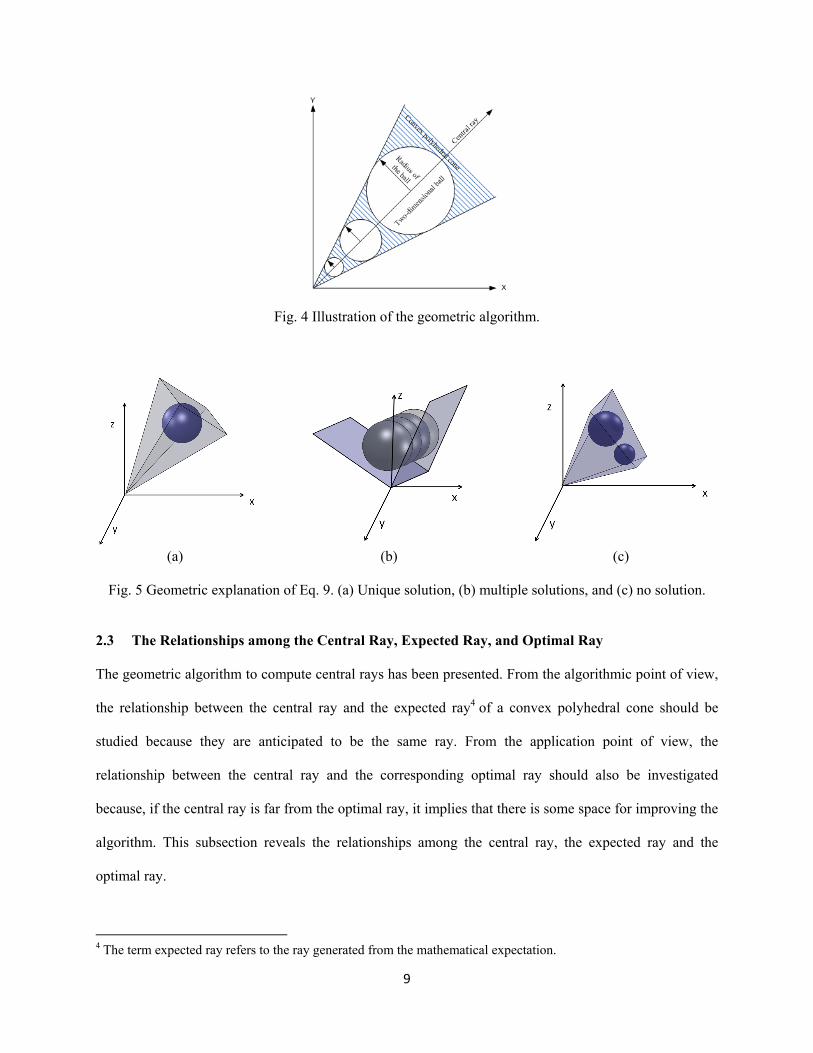
In this subsection, a simple geometric algorithm3 is derived to estimate the central ray of a convex

polyhedral cone. This algorithm is the realization of the idea that a ball is put into a convex polyhedral

cone. If the ball touches all planes of the cone, it cannot be moved closer to the apex (Fig. 4). By locating

the centers of balls with different radii, the central ray of the cone can be constructed. Let us

mathematically formulate this idea. Given a convex polyhedral cone : 0dC x x Q , a set of

hyperplanes 1 0,q x and 0mq x , where kq is the kth row in Q, can be obtained. Here, we assume

that 0x Q is a minimum representation [24]. Given a point dy , the displacement between y and a

hyperplane 0kq x can be calculated by

/k k kq y q . (8)

3 Although the geometric algorithm was completely designed by the author without help from other materials, he cannot guarantee that there is no other published algorithm for computing the central ray of a convex polyhedral cone because geometry is a large field with many years of history and many other fields use it.

8

Note that k is displacement, not distance, and 0k when y C . Rewriting Eq. 8 gives k k kq y q .

Let us seek a point with the same displacement to all hyperplanes, i.e., 1 m . This point is the

center of a hypersphere with radius , which touches all hyperplanes. Using the matrix representation,

we obtain

1

m

q

y

q

Q , (9)

where 0 . As with other linear systems, Eq. 9 can have unique, multiple, or no solutions. Eq. 9 has a

unique solution, meaning that there exists only one position in the cone such that the hypersphere can

touch all hyperplanes. Eq. 9 has multiple solutions, meaning that there exists more than one position in

the cone such that the hypersphere can touch all hyperplanes. Eq. 9 has no solution, meaning that no such

position exists in the cone. Fig. 5 illustrates these three cases.

We use the center of the hypersphere to determine the central ray of the convex polyhedral cone.

Let y be a solution of Eq. 9 for a hypersphere with radius . It is easily proven that y , where 0 , is

also a solution for a hypersphere with radius . Each solution of Eq. 9 produces one central ray, i.e.,

y . Any point on the ray is the center of a hypersphere, which touches all hyperplanes. If Eq. 9 has no

solution, the least square method can compute y.

One may suggest generalizing skeletonization algorithms, which were designed for digital

images, from two-dimensional to d-dimensional domains to find the central ray. It is an ineffective

approach because these algorithms have to discretize the d-dimensional solution space and label all the d-

dimensional voxels in it. Note that the solution space is unbounded, which makes it impossible to label all

the voxels in the solution space. In other words, only a subset of voxels can be labeled. If they are not

selected appropriately, the central ray cannot be obtained, even for over-constrained systems. For under-

constrained systems, this problem is more obvious.

9

Fig. 4 Illustration of the geometric algorithm.

(a)

(b)

(c)

Fig. 5 Geometric explanation of Eq. 9. (a) Unique solution, (b) multiple solutions, and (c) no solution.

2.3 The Relationships among the Central Ray, Expected Ray, and Optimal Ray

The geometric algorithm to compute central rays has been presented. From the algorithmic point of view,

the relationship between the central ray and the expected ray4 of a convex polyhedral cone should be

studied because they are anticipated to be the same ray. From the application point of view, the

relationship between the central ray and the corresponding optimal ray should also be investigated

because, if the central ray is far from the optimal ray, it implies that there is some space for improving the

algorithm. This subsection reveals the relationships among the central ray, the expected ray and the

optimal ray.

4 The term expected ray refers to the ray generated from the mathematical expectation.

10

To study their relationships, a distribution of rays has to be defined. Let C be a convex polyhedral

cone, : 0dC x x Q , where each row of Q is normalized, i.e., 11 dqq and Q is an

invertible d by d matrix. Thus, its central ray 5 cR can be calculated by 1cR Q , where

[1 1 1] .T Let Rr be a random ray generated by

1rR Q , (10)

where 1[ ]Td and 1, , d are independent and identically distributed random variables

following a distribution with a probability density function f whose mean is and support is ][ ba .

Thus, the probability density of is 1

( )d

ii

f . Note that 0a . All random rays generated by Eq. 10

are in the convex polyhedral cone C. i represents the distance between the point that is used to construct

a random ray and the hyperplane 0xqi .

Let Rt be a target ray for C. In the following sections, Rt represents the original features and

images. Note that Rt is an unknown. Without other prior knowledge, each ray in C can be the target ray.

Assuming that Rt follows the distribution generated by Eq. 10, an optimal ray Ro is defined

arg max ( )To t

RR R R p d

, subject to 1R , (11)

where ( )p represents the probability density of . The expected inner product is used as an objective

function because many biometric methods, including the variants of IrisCode, use the inner product to

measure the similarity between an input biometric signal (e.g., iris image) and a filter (e.g., Gabor filter)

as a feature extractor. Thus, Eq. 11 uses the inner product to measure the similarity between R and tR .

If the norm of R is not constrained, max ( )TtR R p d approaches infinity. Rewriting Eq. 11,

arg max ( )To t

RR R R p d

, subject to 1R , (12)

5 In the subsection, the term ray also refers to the point that generates the ray.

11

can be achieved. Clearly, ( )tR p d is the expected ray, and the optimal ray of this objective function is

( ).

( )

t

o

t

R p dR

R p d

(13)

Thus, the optimal ray and the expected ray are the same ray.

Now, we show that the central ray is the expected ray as well as the optimal ray. Substituting Eq.

10 into ( )tR p d , we can obtain

1 ( )p d Q . (14)

Simplifying Eq. 14, 1 1( )p d Q Q , which is the central ray, is derived. Thus, the central

ray, the expected ray, and the optimal ray of the objective function on the distribution are the same ray. In

this derivation, we do not specify the probability density function f , so a group of probability density

functions, including a uniform distribution can be employed as f .

For over-constrained systems, the previous random model is not well defined because it is not

necessary to have an Rt such that tR Q , where Q is an over-constrained matrix. Thus, the random

model has to be revised. Using the least square method, 1T TtR

Q Q Q can be achieved. For the

sake of convenience, let 1

2T T

L

Q Q Q Q . Replacing Rt in Eq. 11 with tR

~, we can obtain an optimal

ray 2 2/L L Q Q , which is also the expected ray, for the objective function,

arg max ( )To t

RR R R p d

, subject to 1R . (15)

For under-constrained systems, there is more than one Rt satisfying ˆtR Q , where Q is an

under-constrained matrix. Let †Q be the Moore-Penrose pseudoinverse of Q and †ˆtR Q . In the

following experiments, the Moore-Penrose pseudoinverse was also used for under-constrained systems.

12

Replacing Rt in Eq. 11 with ˆtR , we can derive that the optimal ray † †/ Q Q , which is also the

expected ray, for the objective function,

ˆarg max ( )To t

RR R R p d

, subject to 1R . (16)

Thus, for all the cases, the central ray is the expected ray as well as the optimal ray.

3. Convex Polyhedral Cones in Different Biometrics Templates

This section shows that templates produced by IrisCode and GIrisCodes are convex polyhedral cones in

different hyperspaces and provides an algorithm to project these cones into a lower-dimensional space to

find a unique solution for Eq. 9 for iris and palmprint templates. Additionally, an algorithm based on the

intersection of convex polyhedral cones is also offered to demonstrate that protected templates are

vulnerable.

3.1. IrisCode and its Low-Order Generalization

Let us consider IrisCode first. Using the notations provided in Section 2, we can derive the inequalities

ˆ 0Tjr jrb g I and ˆ 0T

ji jib g I , where ˆ 2( 0.5)jr jrb b and ˆ 2( 0.5)ji jib b from Eqs. 1-4. ( )ˆ 1jr ib

when ( ) 1jr ib and ( )ˆ 1jr ib when ( ) 0jr ib . The notation r(i) signifies either real or imaginary part

from the Gabor filter. Each bit in an IrisCode generates one inequality, which associates with a

hyperplane, i.e., ( ) ( )ˆ 0T

jr i jr ib g x . Putting these inequalities into a matrix form, we obtain ˆ 0Tb

I Ψ ,

where ˆ 1 1 1 1ˆ ˆ ˆ ˆ[ , , , , , ]r r nr nr i i ni nibb g b g b g b gΨ and n=1024. An IrisCode is clearly a convex polyhedral

cone. b

Ψ is an N by 2048 matrix, where N equals the total number of pixels in a normalized iris image.

The central ray of this convex polyhedral cone can be obtained by solving the linear system ˆT

bI Ψ ,

where [1 1 1]T and 0 , because all ( )sjr ig have been normalized, i.e., ( ) 1jr ig . It is clearly an

13

under-constrained system, because 2048N . In our experiments, N is 32,768. The result in Section 2

pinpoints that if y is a solution of the linear system for a hypersphere with radius , y , where 0 ,

is also a solution of the linear system for the hypersphere with radius . We can thus set 1 .

Rewriting the linear system, we obtain

ˆT I BΨ , (17)

where 1 1ˆ ˆ ˆ ˆˆ [ , , , , , ]T

r nr i niB b b b b and 1 1[ , , , , , ]r nr i nig g g gΨ 6 . Eq. 17 has multiple solutions,

because it is still an under-constrained linear system.

We now seek a particular solution for Eq. 17. Using the results in [20], I can be decomposed as

2 1

1 1 1

n n N n

jr jr ji ji j j Nj j j

I a g a g c t

, (18)

where jra , jia , jc and t , [1 1 1]TN , j

is a unit vector orthogonal to N and all krg and

,kig i.e., ( ) 0Tj kr ig and 0T

j N , where 1 k n . Note that N and are different in size. Eq. 18

can be simplified as

2 1

1

N n

j j Nj

I A c t

Ψ , (19)

where 1 1[ ]Tr nr i niA a a a a . Note that 0T

j Ψ and 0T

N Ψ , where 0s are zero vectors.

Substituting Eq. 19 and ˆ 2( 0.5 )B B , where 1 1[ , , , , ]Tr nr i niB b b b b , into Eq. 17, we obtain

2( 0.5 )T A B Ψ Ψ , (20)

where

6 The matrix can be downloaded from http://goo.gl/mv2EF.

14

1 1 1 1 1 1

1 1

1 1 1 1 1 1

1 1

T T T Tr r r nr r i r ni

T T T Tnr r nr nr nr i nr niT

T T T Ti r i nr i i i ni

T T T Tni r ni nr ni i ni ni

g g g g g g g g

g g g g g g g g

g g g g g g g g

g g g g g g g g

Ψ Ψ

. (21)

Let Ι Α= Ψ . If TΨ Ψ is invertible, we obtain

1ˆ 2( 0.5 )TI B

Ψ Ψ Ψ . (22)

Clearly, I in Eq. 22 is a solution of Eq. 17. Substituting Eq. 19 into the original convex polyhedral cone

ˆ 0Tb

I Ψ , we obtain another convex polyhedral cone ˆ 0Tb

A Ψ Ψ with a lower dimension. The

original cone is projected into the lower-dimensional space because our previous results indicate that the

space spanned by the Gabor filters 1 1, , , , ,r nr i nig g g g stores rich iris information [20]. Another two

points should be mentioned. This derivation uses neither prior knowledge from iris images nor any

special IrisCode structure. Templates produced by other biometric methods that use

1 0j jb if f Id d

, (23)

0 0j jb if f Id d

, (24)

where jb is a bit in their feature codes and jf represents their filter, as a feature extractor are also convex

polyhedral cones, and Eq. 22 can compute their central rays. Note that I in Eqs. 23-24 is a two

dimensional image. Column vectors in the corresponding Ψ should be normalized. Eq. 22 can be

implemented in one MATLAB command line, if memory is enough. If other methods can recognize I ,

the simplicity of Eq. 22 significantly deepens our concern for privacy, because it implies that junior

hackers with neither advanced image processing knowledge nor biometric databases can still reveal

relationships among templates produced by different recognition methods. Ψ is not a secret for many

methods, because researchers disclosed their Ψ s in their papers.

15

3.2. The High-Order Generalization of IrisCode

The previous subsection has pinpointed that templates produced by IrisCode and other biometric methods

that use Eqs. 23 and 24 as feature extractors are convex polyhedral cones in different hyperspaces. This

subsection shows that templates produced by methods that are high-order IrisCode generalizations are

also convex polyhedral cones, including Competitive Code and its variants for palmprint, vein and finger-

knuckle recognition and precise phase representation [4-5, 10].

The feature extractor of these algorithms can be summarized as

,0

arg max Tj j k

k Sh I

, (25)

where j is a feature value to be encoded, ,j kh is a filter, and S is the total number of filters used to

compute one feature value. j can be encoded by a specially designed code table such that it can be

represented in a binary format and hamming distance can be used for matching [4]. Each feature value is

computed from a group of filters, i.e., ,0 , 1, ,j j Sh h . Competitive Code uses six real parts of Gabor filters

with different orientations [5]. In other words, for Competitive Code, S is equal to 6 and ,j ih is a real part

of a Gabor filter. S-1 inequalities, , , ,j

T Tj k jh I h I where j k , can be derived from Eq. 25 for each

feature value. Rewriting the inequalities, we obtain , ,( ) 0j

Tj k jh h I . For convenience, let 0j and

, , ,( )jj k j j kh h h . Using a matrix presentation, a linear inequality system 0T I , where

1,1 , 1[ ]J Sh h , can be obtained. Templates produced by Eq. 25 are clearly also convex polyhedral

cones. If , 0Tj kh I , then , ,( ) / 0T

k j j kh I h . Using this fact, another inequality system ˆ 0T I , where

1,1 1,1 , 1 , 1ˆ / /J S J Sh h h h

, can be derived.

The central ray of this convex polyhedral cone can be determined by solving the matrix equation

ˆ T I . As in the previous subsection, let 1

, , ,1 1

/J S

j s j s j s j jj s j

I u h h w

, where ,j su and

16

jw and , 0, , and .Tj s kh j s k Substituting

1

, , ,1 1

/J S

j s j s j s j jj s j

I u h h w

into ˆ T I , we

obtain ˆ ˆT U , where 1,1 , 1[ ]TJ SU u u . If 1ˆ ˆT

exists, 1ˆ( )TU . Let ˆI U ,

which is an approximation of I. Substituting 1ˆ ˆ( )TU into ˆI U , we obtain

1ˆ ˆ ˆ( )TI . (26)

After constructing , Eq. 26 can also be implemented in one MATLAB command line.

3.3. Using the Intersection of Convex Polyhedral Cones to Break into Protected Templates

Biohashing, a cancelable biometric method modified from IrisCode, was designed for template protection

[16-17]. Once a template is compromised, Biohashing attempts to reissue a new template. It is expected

that Biohashing can issue new templates without limit, compromised templates cannot be matched with

newly issued templates, and the original biometric signal cannot be revealed from compromised

templates. In this subsection, we first show that templates produced by Biohashing are also convex

polyhedral cones. We then provide an algorithm estimating the central ray in the intersection of convex

polyhedral cones from compromised templates to reveal the protected biometric signal.

Biohashing uses the same computational step as IrisCode to produce protected feature vectors.

Given an original feature vector v, Biohashing uses a random matrix, 1[ , , ]m

with size n by

m and m n , whose 0Tk j , k j , 1k and 1T

k k k , to project v into a lower-

dimensional random subspace, i.e., TcW v and further binarizes Wc as with Eqs. 1-4. In summary,

each bit in a protected feature vector can be computed through

0

1

Tj

j Tj

if vw

if v

, (27)

where was set to zero in the experiments [16]. If one template is compromised, Biohashing replaces the

random matrix with another random matrix. It is expected that the original feature vector in a

17

protected template cannot be revealed, even if attackers obtain . Some researchers attempted to break

into the protected templates [25-26]. Our experimental results show that if the system threshold is high

enough, Biohashing can defend their attacks. Using the result in Section 3.1, we can easily derive the

convex polyhedral cone of Biohashing, i.e., ˆ | 0m TV x x , where 1 1

ˆ ˆ ˆ[ , , ]m mw w

and ˆ 2( 0.5)j jw w . As k has been normalized, i.e., 1k , the central ray of this convex polyhedral

cone can be determined by solving the linear system

2( 0.5 )T v W , (28)

where 1[ , , ]TmW w w

. The derivation of Eq. 28 is same as Eq. 17. Clearly, it is still an under-

constrained linear system. However, if an attacker obtains e compromised templates generated from the

same biometric signal and corresponding random matrixes 1 1, e and e , they can simultaneously

reveal the original biometric signal and finally break into the system. Let the convex polyhedral cone

associated with k be ˆ: 0k

m TkV x x

. All convex polyhedral cones must contain the original

biometric signal. In other words, the original biometric signal must be in the intersection of all convex

polyhedral cones. The intersection is also a convex polyhedral cone defined as

1

1ˆ

: 0

ˆe

T

m

Te

V V x x

. (29)

Clearly,

1 1 1 1 2 1( ) ( ) ( )

e ev V V V V V V V

. (30)

Eq. 30 implies that when e increases, the size of the convex polyhedral cone 1 e

V V decreases. If

the convex polyhedral cone is small enough, we can use its central ray to approximate the original

18

biometric signal. If 1

ˆ

0

ˆ

T

Te

x

is a minimum representation, the central ray of the intersection can be

obtained by solving the linear system

11

2 0.5

e

T

Te

W

v

W

. (31)

In the experiments, we used the Moore-Penrose pseudoinverse to solve Eq. 31. To keep the simplicity of

the algorithm and simulate junior hackers breaking into Biohashing, we did not use any methods to

remove redundant constraints.

4. Experimental Results

Two iris databases, the UBIRIS.v1 and West Virginia University (WVU) iris databases [27-28], and one

palmprint database were used to test the proposed algorithms. The UBIRIS.v1 database contains 1,877

images from 241 irises, and the WVU7 iris database contains 3,099 iris images from 472 irises. All

images in the WVU iris database were tested in the experiments. However, 48 images from the

UBIRIS.v1 database were automatically removed, because of their poor quality (Fig. 6). Though some

extremely low-quality images were discarded, many challenging iris images were retained for evaluation.

Fig. 7 gives some examples of the challenging images. The UBIRIS.v1 iris images were taken under a

visible lighting environment, while the WVU iris images were taken under an infrared lighting

environment. The original images in the UBIRIS.v1 database are color images. We only used their red

component for evaluation, because the iris texture in this component is the clearest (Fig. 8). The palmprint

database contains 7,500 images from the right and left palms of 250 persons. Each palm has 15 images in

the database. Ten images were collected in the first session, and the others were collected in the second

session. The left palm images were flipped, so all images in this database could be regarded as right

7 Some mislabeled images were corrected.

19

palms. The central parts of these palmprints were extracted [29]. Fig. 9 gives some examples of the

preprocessed palmprints.

Fig. 6 Examples of the discarded iris images in the UBIRIS.v1 database.

Fig. 7 Examples of low-quality iris images for evaluation.

(a) (b) (c) (d)

Fig. 8 Iris texture in different components. (a) is a color image; (b)-(d) are the R, G and B components of (a), respectively.

Fig. 9 Examples of preprocessed palmprints. 4.1. Evaluation of Iris Recognition Methods

In this section, six iris recognition methods, IrisCode [2], SVM [11], and Ordinal Code (Di-lobe d=5 and

d=9 and Tri-lobe d=9 and d=17) [9], were re-implemented to evaluate the proposed algorithm derived in

Section 3.1 in terms of Receiver Operating Characteristic (ROC) curves. Masks that denote noise pixels,

20

such as eyelids and eyelashes, were used to exclude corrupted bits in all templates generated by these

methods. The raw hamming distances of the Ordinal Code were rescaled to those in IrisCode [4]. From

each database, 90 images were used to train the SVM with a Gaussian kernel [11]. The proposed

algorithm estimated the central rays of IrisCode and Ordinal Code. Ordinal Code is a low-order

generalization of IrisCode. For the central rays of IrisCode, the SVM approach was used as a tester. We

matched the central rays of IrisCode with the original images using the SVM approach. The central rays

of Ordinal Code used IrisCode as a tester. We matched the central rays of Ordinal Code with the original

images using IrisCode. In each set of experiments, cross-matching between all original images was first

performed, and the corresponding genuine and imposter distributions were estimated. The central rays

were then matched with their parent8 images and all other iris images from the same eye. Two genuine

distributions were obtained. The imposter distributions from the cross-matching between the original

images and all genuine distributions were used to plot ROC curves. For the same database and method, all

ROC curves were generated from the same imposter distribution that determines the false acceptance rate

of a system when a threshold is given. This experimental setting studies the risk of using the central rays

to break into the systems. For example, attackers can submit a central ray of a compromised template into

the data link between a biometric sensor and feature extractor, and if they can stop the liveness detector

and quality checker, they can use the central ray to perform a sensor-level break-in [32]. Note that the

theory given in this paper can guarantee that an IrisCode computed from an original image and an

IrisCode computed from the corresponding central ray are no different. Thus, it is impossible to

distinguish them at the matcher level. For convenience, the ROC curves from the cross-matching between

the original images are called original ROC curves, the ROC curves from matching the central rays with

their parent images are called parent ROC curves, and the ROC curves from matching the central rays

with the original images are called resultant ROC curves. Fig. 10 illustrates the matching processes. Figs.

11 and 12 show the ROC curves of the SVM approach and IrisCode, respectively. All parent ROC curves

are above the corresponding original ROC curves, indicating that the errors introduced by the central rays

8 A parent image of a central ray is an image producing a biometric template that is used to compute the central ray.

21

are smaller than those in the original images. If a compromised template and template in a database are

generated from the same iris image, the central ray of the compromised template performs even better

than other iris images from the same eye. If the central ray and template are not generated from the same

image, there is a 70% to 85% chance to break into the systems when the thresholds are set at false

acceptance rate of 0.001. Using Eq. 22, it can be proven easily that if a central ray is obtained from an

IrisCode (Ordinal Code) and IrisCode (Ordinal Code) is used as a matcher, the central ray does not

introduce any additional error bits. The central ray can break into an iris recognition system running

IrisCode (Ordinal Code) if attackers can stop its liveness detector and quality checker or submit the

central ray into the data link between its sensor and feature extractor.

Fig. 10 Illustration of three different matching processes. The blue, black and red arrows indicate respectively the processes of computing genuine matching scores for original, resultant and parent ROC curves.

(a) (b) Fig. 11 ROC curves of the SVM method. The iris images were estimated from the convex polyhedral cones of IrisCode. (a) The results from the UBIRIS.v1 database and (b) the results from the WVU iris database.

10-1

100

101

102

80

82

84

86

88

90

92

94

96

98

100

False acceptance rate (%)

Gen

uine

acc

epta

nce

rate

(%

)

Original SVM ROCResultant ROC (IrisCode vs SVM)Parent ROC (IrisCode vs SVM)

10-1

100

101

102

80

82

84

86

88

90

92

94

96

98

100


Gen

uine

acc

epta

nce

rate

(%

)

Original SVM ROCResultant ROC (IrisCode vs SVM)Parent ROC (IrisCode vs SVM)

22

(a) (b)

(c) (d)

(e) (f)

10-2

10-1

100

101

102

40

50

60

70

80

90

100


Gen

uine

acc

epta

nce

rate

(%

)

Original IrisCode ROC

Resultant ROC (Ordinal Code di-lobe (d=5) vs IrisCode)Parent ROC (Ordinal Code di-lobe (d=5) vs IrisCode)

10-2

10-1

100

101

102

40

50

60

70

80

90

100


Gen

uine

acc

epta

nce

rate

(%

)

Original IrisCode ROCResultant ROC (Ordinal Code di-lobe (d=5) vs IrisCode)Parent ROC (Ordinal Code di-lobe (d=5) vs IrisCode)

10-2

10-1

100

101

102

40

50

60

70

80

90

100


Gen

uine

acc

epta

nce

rate

(%

)


10-2

10-1

100

101

102

40

50

60

70

80

90

100


Gen

uine

acc

epta

nce

rate

(%

)


10-2

10-1

100

101

102

40

50

60

70

80

90

100


Gen

uine

acc

epta

nce

rate

(%

)

Original IrisCode ROCResultant ROC (Ordinal Code tri-lobe (d=9) vs IrisCode)Parent ROC (Ordinal Code tri-lobe (d=9) vs IrisCode)

10-2

10-1

100

101

102

40

50

60

70

80

90

100


Gen

uine

acc

epta

nce

rate

(%

)


23

(g) (h) Fig. 12 ROC curves of the IrisCode. The first column presents the results from the UBIRIS.v1 database, and the second column presents the results from the WVU iris database. Rows 1-4 are results from iris images estimated from the convex polyhedral cones of di-lobe (d=5), di-lobe (d=9), tri-lobe (d=9) and tri-lobe (d=17), respectively.

4.2. Evaluation of Palmprint Recognition Methods

In this section, three palmprint recognition methods, Competitive Code [5], Fusion Code [31], and

PalmCode [29], were re-implemented to evaluate the algorithm presented in Section 3.2. Competitive

Code is a high-order generalization of IrisCode. In this experiment, the central rays of Competitive Code

were matched with the original images using Fusion Code and PalmCode. Five thousand palmprint

images in the database were tested. Half of the images were collected in the first session, and the rest

were collected in the second session. This experiment studied the risk of using the central rays to reveal

relationships among templates produced by different palmprint identification methods. If templates

produced by different methods can be matched, user privacy can be invaded, because the same person

registered in different systems can be known. If a hamming distance of Fusion Code or PalmCode,

obtained by matching the central ray of a Competitive Code with an original image, is significantly

shorter than other hamming distances from matching the central ray with other images, the Competitive

Code and original image can be regarded as from the same palm. The imposter distributions from the

cross-matching between the central rays of Competitive Code, and original images, and corresponding

genuine distributions were used to plot ROC curves. Fig. 13 shows the Fusion Code and PalmCode ROC

10-2

10-1

100

101

102

40

50

60

70

80

90

100


Gen

uine

acc

epta

nce

rate

(%

)


10-2

10-1

100

101

102

40

50

60

70

80

90

100


Gen

uine

acc

epta

nce

rate

(%

)


24

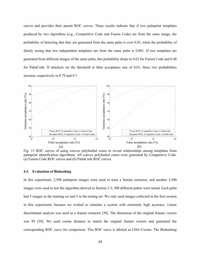
curves and provides their parent ROC curves. These results indicate that if two palmprint templates

produced by two algorithms (e.g., Competitive Code and Fusion Code) are from the same image, the

probability of detecting that they are generated from the same palm is over 0.83, when the probability of

falsely seeing that two independent templates are from the same palm is 0.001. If two templates are

generated from different images of the same palm, this probability drops to 0.62 for Fusion Code and 0.48

for PalmCode. If attackers set the threshold at false acceptance rate of 0.01, these two probabilities

increase, respectively to 0.79 and 0.7.

(a) (b) Fig. 13 ROC curves of using convex polyhedral cones to reveal relationships among templates from palmprint identification algorithms. All convex polyhedral cones were generated by Competitive Code. (a) Fusion Code ROC curves and (b) PalmCode ROC curves. 4.3. Evaluation of Biohashing

In this experiment, 2,500 palmprint images were used to train a feature extractor, and another 2,500

images were used to test the algorithm derived in Section 3.3; 500 different palms were tested. Each palm

had 5 images in the training set and 5 in the testing set. We only used images collected in the first session

in this experiment, because we wished to simulate a system with extremely high accuracy. Linear

discriminant analysis was used as a feature extractor [30]. The dimension of the original feature vectors

was 99 [30]. We used cosine distance to match the original feature vectors and generated the

corresponding ROC curve for comparison. This ROC curve is labeled as LDA+Cosine. The Biohashing

10-1

100

101

102

40

50

60

70

80

90

100


Gen

uine

acc

epta

nce

rate

(%

)

Parent ROC (Competitive Code vs Fusion Code)

Resultant ROC (Competitive Code vs Fusion Code)

10-1

100

101

102

40

50

60

70

80

90

100


Gen

uine

acc

epta

nce

rate

(%

)

Parent ROC (Competitive Code vs PalmCode)

Resultant ROC (Competitive Code vs PalmCode)

25

template sizes were 60 and 90 bits. Each testing image was matched with 5 training images from the same

palm to produce five hamming distances, and the smallest distance was considered a genuine hamming

distance. Similarly, each testing image was matched with all other images. The minimum hamming

distance from the same palm in the database was considered an imposter hamming distance. The

corresponding ROC curves were labeled as Biohashing (K bits), where K is the number of bits in the

templates. We also estimated the central rays of the intersection of the convex polyhedral cones formed

by compromised Biohashing templates to match newly reissued templates. More clearly, we matched the

11[ , , ]

q

TmW w w

generated from an original image with the 1

1ˆ ˆ ˆ[ , , ]

q

TmW w w

generated from an

estimated central ray, where 1q represents a newly re-issued random matrix. We only matched W with

W from the same palm. Only genuine distributions were produced from these matches. Using these

genuine distributions with the original Biohashing impostor distributions, the probability of a break-in

based on the central rays of the intersections of the convex polyhedral cones formed by compromised

templates can be estimated. The ROC curves generated from the original impostor distributions and these

genuine distributions are referred to as the ROC curves of the CPC algorithm (CT), where CT denotes the

number of compromised templates used to compute the central rays. We also implemented a constrained

optimization method for comparison [26]. To estimate the original biometric vectors protected by

Biohashing, this method uses information from unrelated feature vectors (e.g., from different persons). In

this experiment, each original vector was estimated by 100 feature vectors from 100 different palms.

When the number of comprised templates is one, the CPC algorithm is same as our previous work [25].

However, we neither discussed convex polyhedral cones nor used multiple compromised templates to

estimate original feature vectors in that work [25]. Fig. 14 shows the ROC curves, clearly indicating that

the CPC algorithm can effectively break into Biohashing. The probability of a successful break-in is over

40% when the central rays are estimated from only 7 compromised templates with 60 bits and system

threshold is set at false acceptance rate of 0.001%; the probability of a successful break-in is over 50%

when the central rays are estimated from only 4 compromised templates with 90 bits and system threshold

26

is set at false acceptance rate of 0.001%. As the number of compromised templates increases, the

probability of a successful break-in also increases. When the number of compromised templates is

enough, the CPC algorithm can perform even better than the original Biohashing.

As mentioned above, Biohashing can defend attacks from the constrained optimization method if

the decision threshold is high enough [26]. Readers may wonder why the constrained optimization

method cannot perform better than the CPC algorithm (CT=1) if both use information from one

compromised template, but the constrained optimization method utilizes additional images from other

palms to estimate the original features. This phenomenon can be explained by the geometric structure of a

convex polyhedral cone. The constrained optimization method has two steps. Given a set of unrelated

feature vectors 1 K , this method seeks a solution kx that has a minimum distance from k and

fulfills all constraints from a compromised template. Mathematically, kx is obtained from optimizing

argmin subject to 0 if 0 and 0 if 1 T Tk k j j j j

xx x x w x w j , (32)

where jw is a bit in a compromised template and j is a column vector from the compromised random

matrix. Note that both Eq. 32 and the CPC algorithm require information from the compromised random

matrix Ω. After obtaining kx s, the constrained optimization method computes the weight average, i.e.,

2

1

2

1

/

1 /

K

k kk

f K

kk

x d

x

d

, (33)

where dk is the hamming distance between the Biohashing templates of k and kx . To understand why

this constrained optimization method cannot surpass the CPC algorithm (CT=1), let us consider the case

of only one unrelated feature 1 first. Because K=1, we can derive that 1.fx x Note that 1 is a feature

from another person and 1 therefore cannot fulfill all constraints in Eq. 27, i.e., j such that 1 0Tj

if 1 jw or 1 0Tj

if 0 jw . In other words, 1 is not inside the convex polyhedral cone of the

compromised template. The solution obtained from Eq. 32 is on the boundary of the convex polyhedral

27

cone (Fig. 15). If more than one unrelated feature is used, the final solution xf is a weighted average of a

set of points on the boundary of the convex polyhedral cone. It can be considered as a method of

estimating the central ray of the convex polyhedral cone. If the unrelated feature vectors are used

appropriately, methods that outperform the CPC algorithm (CT=1) are likely to be developed [20].

(a) (b) Fig. 14 ROC curves of using convex polyhedral cones to attack Biohashing with (a) 60 bits and (b) 90 bits.

Fig. 15 Illustration of the phenomenon that the CPC algorithm (CT=1) and the constrained optimization method perform similarly.

5. Discussion

Though the number of theoretical properties of IrisCode has recently been discovered, our understanding

of this influential iris recognition algorithm remains incomplete. In this paper, we indicate that templates

10-3

10-2

10-1

100

101

102

0

10

20

30

40

50

60

70

80

90

100

False acceptance rate %

Gen

uine

acc

epta

nce

rate

%

Biohashing (60 bits)LDA+CosineCPC Algorithm (CT=1)CPC Algorithm (CT=3)CPC Algorithm (CT=5)CPC Algorithm (CT=7)CPC Algorithm (CT=9)CPC Algorithm (CT=12)CPC Algorithm (CT=16)CPC Algorithm (CT=20)Constrained optimization

10-3

10-2

10-1

100

101

102

0

10

20

30

40

50

60

70

80

90

100

False acceptance rate %

Gen

uine

acc

epta

nce

rate

%

Biohashing (90 bits)FDA+CosineCPC Algorithm (CT=1)CPC Algorithm (CT=2)CPC Algorithm (CT=3)CPC Algorithm (CT=4)CPC Algorithm (CT=5)CPC Algorithm (CT=6)CPC Algorithm (CT=7)CPC Algorithm (CT=8)CPC Algorithm (CT=9)Constrained optimization

28

produced by IrisCode and its generalization are convex polyhedral cones. From a geometric perspective,

IrisCode cuts down the hyperspace formed by normalized iris images into 22048 convex polyhedral cones.

Each convex polyhedral cone represents one iris template, but an iris is represented by a set of convex

polyhedral cones that are near in terms of hamming distance.

Using the geometric properties of convex polyhedral cones, a simple algorithm that can often be

implemented in one MATLAB command line has been developed to estimate the central rays of IrisCode

and GIrisCode. The experimental results show that these central rays can match iris and palmprint

templates produced by different methods and break into protected biometric templates. They imply that

the central rays are enough to reveal the relationships among templates produced by different methods

and break into systems without liveness detectors and quality checkers and that Biohashing has a limited

capability to reissue new templates. The central rays of a compromised template can also be submitted

into the data link between a biometric sensor and a feature extractor [32]. Except for replay attack at the

sensor level, all other attacks do not depend on the visual quality of the preprocessed images (iris image)

generated from the central rays. For some methods, central rays are, in fact, preprocessed images with

reasonable visual quality. Fig. 16 shows preprocessed images generated from the central rays of Ordinal

Codes (di-lobe d=5). The DC and the contrast of the original images are used to display the central rays to

avoid visual differences caused by these two factors. Because Ordinal Code uses only the left and the

right parts of an iris, Fig. 16 only shows these two parts [9].

Without solid security analyses, any biometric template that is a convex polyhedral cone cannot

be assumed to be secure. The simplicity of the geometric algorithm implies that even junior hackers

without advanced image processing knowledge can invade a system. Even worse, the central ray is also

the expected ray and the optimal ray of an objective function on a group of distributions. Finally, it should

be re-emphasized that this paper aims not to reconstruct high quality images from templates but instead to

provide a deeper understanding of the geometric structures of IrisCode and its variants and investigate the

risk from this geometric information.

29

Fig. 16 Visual comparison between the original images and the central rays of Ordinal Code (di-lobe d=5). The first column presents the original images, and the second column presents preprocessed images from the central rays.

Acknowledgements

We would like to thank the University of West Virginia, the University of Beira Interior and the Hong

Kong Polytechnic University for sharing their databases, Prof. Daugman for his valuable comments, and

Mr. Jose Thomas Thayil for drawing all three-dimensional figures. This work is partially supported by

Academic Research Fund Tier 1 (RG6/10) from the Ministry of Education, Singapore.

References [1] J.G. Daugman, “High confidence visual recognition of persons by a test of statistical independence”,

IEEE TPAMI, vol. 15, no. 11, pp. 1148-1161, 1993. [2] J. Daugman, “How iris recognition works”, IEEE TCSVT, vol. 14, no. 1, pp. 21-30, 2004. [3] J. Daugman, “New methods in iris recognition”, IEEE TSMC, B, vol. 37, no. 5, pp. 1167-1175, 2007. [4] A.W.K Kong, D. Zhang and M. Kamel, “An analysis of IrisCode”, IEEE TIP, vol. 19, no. 2, pp.

522-532, 2010. [5] A.W.K. Kong and D. Zhang, “Competitive coding scheme for palmprint verification”, in Proc.

International Conference on Pattern Recognition, vol. 1, pp. 520-523, 2004. [6] A.K. Jain, S. Prabhakar, L. Hong, and S. Pankanti, “Fiterbank-based fingerprint matching”, IEEE

TIP, vol. 9, no. 5, pp. 846-859, 2000. [7] Z. Sun, T. Tan, Y. Wang and S.Z. Li, “Ordinal palmprint representation for personal identification”,

in Proceedings of IEEE CVPR, vol. 1, pp. 279-284, 2005. [8] L. Ma, T. Tan, Y. Wang, and D. Zhang, “Efficient iris recognition by characterizing key local

variations”, IEEE TIP, vol. 13, no. 6, pp. 739-750, 2004.

30

[9] Z. Sun and T. Tan, “Ordinal measures for iris recognition”, IEEE TPAMI, vol. 31, no. 12, pp. 2211-2226, 2009.

[10] L. Zhang, L. Zhang, D. Zhang and H. Zhu, “Online finger-knuckle-print verification for personal authentication”, Pattern Recognition, vol. 43, pp. 2560-2571, 2010.

[11] H.A Park and K.R. Park, “Iris recognition based on score level fusion by using SVM”, Pattern Recognition Letters, vol. 28, pp. 2019-2028, 2007.

[12] H. Proença and L.A. Alexandre, “Toward noncooperative iris recognition: a classification approach using multiple signatures”, IEEE TPAMI, vol. 29, no. 4, pp. 607- 612, 2007.

[13] E. Krichen, M.A. Mellakh, S. Garcia-Salicetti, and B. Dorizzi, “Iris identification using wavelet packets”, in Proceedings of ICPR, vol. 4, pp. 226-338, 2004.

[14] S.I. Noh, K. Bae, Y. Park and J. Kim, “A novel method to extract features for iris recognition system”, LNCS, Springer, vol. 2688, pp. 861-868, 2003.

[15] W. K. Kong and D. Zhang, “Palmprint texture analysis based on low-resolution images for personal authentication”, in Proceeding of ICPR, pp. 807-810, 2002.

[16] A.T.B. Jin, D.N.C. Ling and A. Goh, “Biohashing: two factor authentication featuring fingerprint data and tokenized random number”, Pattern Recognition, vol. 37, pp. 2245-2255, 2004.

[17] A. Kong, K.H Cheung, D. Zhang, M. Kamel and J. You, “An analysis of Biohashing and its variants”, Pattern Recognition, vol. 39, no. 7, pp. 1359-1368, 2006.

[18] K.P. Hollingsworth, K.W. Bowyer and P.J. Flynn, “The best bits in an iris code”, IEEE TPAMI, vol. 31, no. 6, pp. 964-973, 2009.

[19] A. Kong, “An analysis of Gabor detection”, in Proc. of International Conference on Image Analysis and Recognition, pp 64-72, 2009.

[20] A.W.K. Kong, “IrisCode decompression based on the dependence between its bit pairs”, IEEE TPAMI, vol. 34, no. 3, pp. 506-520, 2012.

[21] B. Grünbaum, Convex Polytopes, Second Edition, Springer-Verlag, New York, 2003. [22] G.M. Ziegler, Lectures on Polytopes, Springer-Verlag, New York, 1995. [23] C.B. Barber, D.P. Dobkin, and H.T. Huhdanpaa, “The quickhull algorithm for convex hulls”, ACM

Transactions on Mathematical Software, vol. 22, no. 4, pp. 469-483, 1996. [24] J. Telgen, “Minimal representation of convex polyhedral sets”, Journal of Optimization Theory and

Applications, vol. 38, no. 1, pp. 1-24, 1982. [25] K.H. Cheung, A.W.K. Kong, J. You and D. Zhang, “An analysis on invertibility of cancelable

biometrics based on BioHashing”, in Proceedings of the International Conference on Imaging Science, Systems, and Technology, pp. 40-45, 2005.

[26] A. Nagar, K. Nandakumar and A. K. Jain, “Biometric template transformation: a security analysis”, in Proc of Media Forensics and Security II, 2010.

[27] H. Proenca and L.A. Alexandre, “UBIRIS: a noisy iris image database”, in Proc. of the 13th International Conference on Image Analysis and Processing, vol. 1, pp. 790-977, 2005.

[28] A. Ross and S. Shah, “Segmenting non-ideal irises using geodesic active contours”, in Proc. of Biometrics Symposium, pp. 1-6, 2006.

[29] D. Zhang, W.K. Kong, J. You and M. Wong, “On-line palmprint identification”, IEEE TPAMI, vol. 25, no. 9, pp. 1041-1050, 2003.

[30] A.B.J. Teoh, A. Goh and D.C.L. Ngo, “Random multispace quantization as an analysis mechanism for Biohashing of biometric and random identity inputs”, IEEE TPAMI, vol. 28, no. 12, pp. 1892- 1901, 2006.

[31] A.W.K. Kong and D. Zhang, “Feature-level fusion for effective palmprint authentication”, in Proceeding of International Conference on Biometric Authentication, pp. 520-523, 2004.

[32] N.K. Ratha, J.H. Connell and R.M. Bolle, “Enhancing security and privacy in biometrics-based authentication systems”, IBM Systems Journal, vol. 40, no. 3, pp. 614-634, 2001.

[33] J. Daugman, Personal Communication.

modeling iriscode and its variants as convex polyhedral

Documents