modeling concordance correlation via gee to evaluate...

BIOMETRICS 57, 931-940 September 2001

Modeling Concordance Correlation via GEE to Evaluate Reproducibility

Huiman X. Barnhart Department of Biostatistics, The Rollins School of Public Health of Emory University,

1518 Clifton Road NE, Atlanta, Georgia 30322, U.S.A. email: [email protected]

and

John M. Williamson Division of HIV/AIDS Prevention: Surveillance and Epidemiology (MS E-48),

National Centers for HIV, STD, and TB Prevention, Centers for Disease Control and Prevention, 1600 Clifton Road NE, Atlanta, GA 30333, U.S.A.

email: [email protected]

SUMMARY. Clinical studies are often concerned with assessing whether different raters/methods produce similar values for measuring a quantitative variable. Use of the concordance correlation coefficient as a measure of reproducibility has gained popularity in practice since its introduction by Lin (1989, Biometrics 45, 255-268). Link method is applicable for studies evaluating two raters/two methods without replications. Chinchilli et al. (1996, Biometrics 52, 341-353) extended Lin’s approach to repeated measures designs by using a weighted concordance correlation coefficient. However, the existing methods cannot easily accommodate covariate adjustment, especially when one needs to model agreement. In this article, we propose a generalized estimating equations (GEE) approach to model the concordance correlation coefficient via three sets of estimating equations. The proposed approach is flexible in that (1) it can accommodate more than two correlated readings and test for the equality of dependent concordant correlation estimates; (2) it can incorporate covariates predictive of the marginal distribution; (3) it can be used to identify covariates predictive of concordance correlation; and (4) it requires minimal distribution assumptions. A simulation study is conducted to evaluate the asymptotic properties of the proposed approach. The method is illustrated with data from two biomedical studies.

KEY WORDS: Agreement; Correlated data; Reliability; Reproducibility.

1. Introduction Accurate and precise measurement is an important component of any proper study design. Before a method, a rater, or an instrument is adopted for use in measuring a variable of interest, a reliability or a validity study is often conducted in clinical or experimental settings. These reliability studies are often concerned with assessing whether different methods/raters produce similar values. The kappa statistic (Co- hen, 1960) and the weighted kappa statistic (Cohen, 1968) are the most popular indices for measuring agreement for discrete outcomes. Traditionally, intraclass correlation (Fleiss, 1986; Quan and Shih, 1996) and within-subject coefficient of variation (Lee, Koh, and Ong, 1989) have been used as indices to evaluate reproducibility. These indices can be estimated by using random-effects models. As elaborated by Lin (1989, 1992), the concordance correlation coefficient is more appropriate for measuring agreement when the variable of interest is continuous. The advantage of this index is that

it includes components of both precision and accuracy. Un- like the concordance correlation coefficient, neither the intraclass correlation coefficient nor the within-subject coefficient of variation contain measurement of accuracy. In general, the correlation coefficient measures the precision component and the ratio of the correlation coefficient and concordance correlation coefficient measures the accuracy component. Several authors (Krippendorff, 1970; Fleiss and Coheri, 1973; Donner and Koval, 1980; Robieson, 1999) noted that the concordance correlation coefficient (or intraclass corrclation coefficient in special cases) computed from ordinal scaled data is equivalent to the weighted kappa when integer scores are used.

Chinchilli et al, (1996) extended Link approach to repeated measures designs by using a weighted concordance correlation coefficient. However, these methods are difficult to use when one would like to model the agreement measure as a function of covariates. Barlow (1996) showed that the estimates of agreement using the kappa coefficient may be inflated if one fails to account for confounding in the marginal distribu-

931

932 Biometrics, September 2001

tion. Similar issues may arise when one uses the concordance correlation coefficient for measuring agreement in the case of a continuous variable. Several authors (Barlow, 1996; Molen- berghs, Fitamaurice, and Lipsitz, 1996; Shoukri and Mian, 1996) have proposed methods to construct inference on kappa while adjusting for covariates through the marginal distribution. However, as noted by Klar, Lipsitz, and Ibrahim (2000) and Gonin et al. (2000), the adjustment in the marginal distribution only produces an overall/summary agreement measure. There are practical needs to compare agreement for mul- tiple or stratified samples, and investigators may wish to “determine and evaluate the strength of agreement taking into account patient-specific (age and gender) as well as rater specific (whether board certified in dermatology) characteristics” (Gonin et al., 2000, p. 1). This suggests modeling agreement as a function of these covariates.

Often, reliability studies will be devised to compare agreement between various methods or instruments used to assess subjects. In addition, a reliability study may be used to evaluate the agreement between a new method and a widely ac- ceptable proven method, a gold standard, which is also measured with error. In these situations, numerous assessments or ratings will be made on the same subject. These measurements will tend to be positively correlated and this correlation must be taken into account to conduct valid inference. Here we focus on the analysis of reliability studies that compare various methods or instruments with correlated continuous measurements assessed on the same subject with adjustment for covariates.

Several authors (Lipsitz and Fitzmaurice, 1996; Molen- berghs et al., 1996) have used generalized estimating equations (GEE) to construct inference on an overall kappa statistic while adjusting for covariates in the marginal distribution. More recently, several approaches have been proposed using GEE equations to model kappa or weighted kappa as a function of covariates (Gonin et al., 2000; Klar et al., 2000; Williamson et al., 2000). In this article, we propose a GEE approach to model both the concordance correlation coefficient and the marginal distribution while adjusting for covariates. The proposed approach is flexible in the sense that (1) i t can accommodate more than two correlated readings; (2) it can easily incorporate covariates predictive of the marginal distribution; (3) it can be used to identify covariates predictive of concordance correlation; and (4) it requires minimal distributional assumptions. In Section 2, we present the proposed GEE approach for modeling the concordance correlation coefficient. A simulation study is conducted to evaluate the asymptotic properties of the proposed approach under small and moderate sample sizes in Section 3. In Section 4, we illustrate the proposed method using two examples. The first example compares three readings using a mercury sphygmomanometer and one reading from an electronic digital instrument in measuring blood pressure. The second example compares two new methods and a gold standard method in evaluating carotid stenosis from a carotid stenosis screening study.

2. Modeling Concordance Correlation via GEE Suppose that J readings are taken on N subjects in a study. These J readings may come from a combination of several raters and several measuring instruments. Let Yi (i = 1,. . . ,

N) be the J x 1 vector that contains the J readings and let the J x p matrix Xi denote the corresponding p covariates for the ith subject. For simplicity, the first column of X i is a vector of all ones representing an intercept term. The covariates can either be subject-specific and/or reading-specific variables. Examples of subject-specific covariates are age, gender, and race. The indicator variables for raters or instruments are examples of reading-specific covariates.

For any two readings Y , and qr (1 5 j , j‘ 5 J, j # j ’ ) , Lin (1989) used the expected squared difference, E[(Y, - Y j r ) 2 ] , scaled between -1 and 1 to define the concordance correlation coefficient as

E [(Y, - Yj,)’] PCj j l = 1 -

u; + u;, + (p j - pjt)2

2Ujj’ - - uj” + u;, + (pLj - p j y

2 where pj = E(Y,), pjt = E ( Y , , ) , ui = var(Y,), uj l = var(Yji), ujj, = cov(yj,Yjt) = u j u j t p j j / , and pj j ’ is the usual correlation between Yj and Yji. Note that p j j i = pcj j l if and only if pj = pjr and uj = uj,. In general, we have -1 5 -1pjjtI 5 pCjj i 5 IpjjrI 5 1 (Lin, 1989).

In order to model concordance correlation, one needs to estimate the means and the variances of Yj and Yjt. Three sets of estimating equations are proposed. Let p be a p x 1 marginal parameter vector. In the first set of equations, we model the marginal mean of Y by E ( Y i ) = pi = X i p , and the parameter estimates of ,B are obtained by GEE as

2 2

N

i=l

where D i = api/dp and Vi is the working covariance matrix for Yi (Zeger and Liang, 1986). In the second set of equations, we estimate the variance of Y . Note that the variances are smaller when one accounts for covariates in the above marginal model. For simplicity, we assume that the variance

and 6$ = E Yi . Then 6? = c2 + p i , where u2 = (u:, . . . , u:)’ with 4 l)var(Yij) and p? = ( P : ~ , . . . , & ) I . We solve the following second set of estimating equations to obtain estimates for c2:

does not depend on covariates. Let Y2 = (y,”,, xi,. . . , y Z J ) 2 ’ 2”

N

i=l

where Fi = a6$/ac2 and Hi is the working covariance matrix for Yi2. In practice, we can use a diagonal matrix for Hi with the j t h component as var(Y,:). If Yi is normally distributed, then we have var(Y;) = 2uj” +4p:jo;. We use this expression as the diagonal component of Hi even if Yi is not normally distributed.

Note that E(Y,Yji) = cov(Yj, qr)+pjp j t = pcj j ’ (s;+u;,+

(pj -p j , )2 ) /2+p jp3 , . This implies that tEe concordance correlation can be obtained once the means and the variances are estimated. Therefore, we use the J ( J - 1)/2 pairwise products YjYj, to model the concordance correlation in a third set of estimating equations. Let Ui = ( y Z l y 2 2 , . . . , y i ( J - l l yZ~) ’ be the J ( J - 1)/2 x 1 vector of the pairwise

Modeling Concordance Correlation 933

products of readings for subject i and denote 8i = E(Ui). Then 8i is a function of u2, pi, and the concordance correlation coefficients (see the expression for E(%%t)). We use Fisher’s 2-transformation to model the concordance correlation coefficient because it ranges between -1 and 1 as

where pcijj’ is the concordance correlation between the j t h and the j’th readings for subject i and Qijji includes a sub- set of covariates in Xi as well as indicator variables for pairs ( j , j ’ ) . For example, if we believe that the concordance correlations among the first three readings are similar, we may pool the information together by using an indicator variable taking value one if the (j l j’) th pair is equal to (1,2), (1,3), or (2,3) and taking the value zero otherwise. We solve for a using the following third set of estimating equations:

N

C c;w;l (ui - ei (alp, g2)) = 0, (3) i=l

where Ci = % i / d a and Wi is the working covariance matrix for Ui. In practice, we use the diagonal matrix for Wi with the (j,j’)th component as var(Y,jqj,). If Yi is distributed as a multivariate normal random variable, then var(xjYijt) = ~ 2 ~ 2 , + p2.~2, + p:j,u; + u;jt + 2pijpijlujj1, where ujjl =

(pcijjt (u;+u;~ +( ,~ i j -p i j i )~ ) ) /2 . We use this expression for a diagonal element in Wi even if Yi is not normally distributed.

Our main interest here is to obtain the parameter estimates of (IY and then the estimates for the concordance correlation coefficients. When there are no covariates, the above estimation process requires no iterations and the resulting concordance correlation estimate is exactly equivalent to Link coefficient. We obtain & by solving three sets of estimating equations. Specifically, we obtain parameter estimates for /3 (p) by using a modified Fisher-scoring iterative procedure,

for the first set of equations. Thus, we have estimates for pi, pi. Replacing pi with pi in the second set of equations, we obtain parameter estimates for u2 (a^2). Finally, we replace pi and u2 with f i i and u2 in the third set of equations and obtain the parameter estimates for a, &. We again used the modified Fisher-scoring iterative procedure for solving the second and third equations. Following similar arguments used for the usual generalized estimating equations (Liang, Zeger, and Qaqish, 1992), we can easily show that the parameter estimates are consistent provided that the three models are correctly specified. This is true whether or not the working correlation matrices in the three sets of equations are correctly specified.

In order to perform inference on the concordance correlations, one needs to obtain estimates for the standard error of 6. Note that 6 is obtained in the third set of equations with estimated p and g2. Therefore, we will need to incorporate the uncertainty in estimating p and u2 in order to obtain the estimates for the standard error of 6. Following Prentice (1988), we can show that the joint asymptotic distribution of N 1 I 2 [ ( j - ,f3)’, (u2 - u2)’, (& - a)’]’ is Gaussian with mean

3 3 2 3 3

p1+1 = pl-{c,N_l Dp2:1Di}-1{Ezl D;v;1(YZ-fii(pl)},

zero and variance matrix as N times

Al l A12 A13 B = *-lA*’-l = 9-1 (A21 A22 A23)

A31 A32 A33

where

*=

N C D!,v;~D~ 0 0 i= l . -

N N

i=l i=l N N N

i=l i=l i = l

with L~ = @/ap, E~ = aei/ap, G~ = aoi/aa2, and

N

Al l = D ’ , V ~ ~ l v a r ( Y i ) V ~ l D i , i=l N

A12 = C D ~ V ; ~ C O V ( Y ~ , Y : ) H Y ’ F ~ , i=l N

A13 = CDIV;’COV(Y~, Ui)W2’1Ci, i=l N

A22 = CFEH,lvar(YS)H;lF,, i= 1 N

A23 = C F : H I ~ C ~ ~ ( Y , ~ , U ~ ) W ; ~ C ~ , i=l N

A33 = CC:W;’var(Ui)WTIC,, i=l

A21 = 4 2 ,

A31 = Ai3i A32 = AL3.

We obtain an estimate for B by replacing the parameters by their corresponding estimates that are the solutions to the estimating equations and estimate the covariances in A by the consistent moment estimates,

var(Yi) = ( ~ i - f i i ) ( ~ i - pi)‘, 2

C O V ( Y i , Yi ) = (Yi - fii)(Y? - &)‘, cov(Y2, UZ) = (Yi - bi)(Ui - &)Il

var(Y:) = (Y: - 6:))~: - J:)’, COV(Yi, Ui) = (Yi - B?)(Ui - &)’, 2 2

var(Ui) = ( ~ i - B,)(u~ - & ) I .

We refer to B as the empirically corrected variance estimate of 6, h2, and 8. The estimate for the variance of $ is obtained by taking the appropriate rows and columns in B. Finally, once we have 6 and the corresponding 95% confidence intervals, the inverse of Fisher’s 2-transformation is used to obtained the estimates for the concordance correlation coefficients and their corresponding confidence intervals. We note that one

934 Biometries, September 2001

Table 1 Results of first set of simulations based o n 500 data setsa

b Pc12

b Pc2

b Pc 1

Mean of Mean of Mean of Type 1 True value est. SE est. SE est. SE error p pc12 Mean (SD) (95% cover.) Mean (SD) (95% cover.) Mean (SD) (95% cover.) rate (%)

0.5 0.7 0.sc

0.5 0.7 O.gd

0.5 0.7 0.9

0.471 0.660 0.848

0.471 0.660 0.848

0.471 0.660 0.848

0.434 (0.182) 0.644 (0.145) 0.872 (0.099)

0.461 (0.109) 0.675 (0.082) 0.895 (0.049)

0.481 (0.078) 0.690 (0.056) 0.897 (0.029)

0.157 (90%) 0.124 (93%) 0.081 (90%)

0.105 (93%) 0.078 (94%) 0.044 (95%)

0.073 (92%) 0.053 (93%) 0.028 (96%)

N = 26 0.460 (0.153) 0.138 (92%) 0.669 (0.119) 0.105 (92%) 0.882 (0.057) 0.048 (93%)

0.476 (0.106) 0.102 (94%) 0.682 (0.080) 0.073 (92%) 0.893 (0.033) 0.030 (95%)

0.486 (0.074) 0.072 (94%) 0.696 (0.053) 0.051 (94%) 0.897 (0.021) 0.021 (97%)

N = 50

N = 100

0.428 (0.134) 0.618 (0.112) 0.824 (0.072)

0.441 (0.092) 0.640 (0.070) 0.840 (0.039)

0.455 (0.062) 0.654 (0.047) 0.845 (0.024)

0.117 (92%)

0.059 (91%) 0.099 (91%)

0.084 (91%) 0.066 (92%) 0.035 (94%)

0.058 (92%) 0.045 (94%) 0.023 (95%)

9.2 9.6 7.6

5.2 6.8 4.0

7.0 5.6 4.0

aData are generated from a six-dimensional multivariate normal distribution with equal means, equal correlations ( p = p C l = p c 2 ) ,

b p c l , pc2, and pc12 are concordance correlation coefficients within methods 1 and 2 and between methods 1 and 2, respectively. and unequal variances (1.0 and 2.0) within methods 1 and 2, respectively.

Convergence occurs in 486 data sets. Convergence occurs in 499 data sets.

may obtain the same estimates of concordance correlation coefficients as Lin’s method when there are no covariates. However, our empirically corrected standard errors may be larger than Link because we don’t make normality assumptions concerning var(Y$) and var(xjY&,) when computing the proposed standard errors.

Noting that E(Y,Y,,) = p j j / u j u j / + p j p j f , it requires minimal effort to model the correlation coefficient as a function of covariates by the same three sets of estimating equations. The estimates of the correlation coefficient can provide insight on whether the poor agreement is due to precision or due to accuracy because the correlation coefficient ( p ) measures the precision and xa = p c / p measures the accuracy.

3. Simulations We conducted analyses using simulated data to assess the performance of our method. We examined the bias of the concordance correlation estimates and determined how well the empirically corrected standard error estimate performs with small to moderate sample sizes with two sets of simulations. We assumed that each subject was assessed by three raters with two methods for both sets of simulations. Let Yi (i = 1,. . . , N ) be the 6 x 1 vector denoting the six readings on subject i from the three raters using methods 1 and 2 (where the first three readings are from method 1). We generated continuous responses, Yi, from a multivariate normal distribution.

For the first set of simulations, we assumed a common mean for the normal random variables, generating each reading with differing variances for each of the two assessment methods, i.e., Yi N N(pi, E) with pij = PO + p lz l i + p 2 z 2 i

for j = 1,. . . , 6 and i = 1,. . . , N . The first covariate, z l i , is a binary subject-specific variable taking a value of zero

for i = 1 , . . . , N/2 and one otherwise. The second covariate, x 2 i , is a continuous subject-specific variable generated as a U(-1, 1) random variable. The values of the parameters generating the data are PO = 0.0 and = pz = 1.0. We assume that the variances of the readings are 1.0 and 2.0 for methods 1 and 2, respectively. The correlation coefficients in the covariance matrix 27 are assumed to be the same and equal to p. Thus, the concordance correlation coefficients within each method are the same and equal to the correlation coefficient p. Let pCl and pc2 be the concordance correlation coefficients for methods 1 and 2, respectively. Then we have pCl = pc2 = p. However, the concordance correlation coefficient (pc.2) measuring the agreement between the two methods is smaller than the correlation coefficient because we assumed differing variances for the two methods. We analyzed 500 data sets of size 26, 50, and 100 ( N ) for the following values of the common correlation coefficient: 0.5,0.7, and 0.9. A test of Ho: pCl = pc2 is performed to check the Type I error rate.

Table 1 summarizes the first set of simulations. The estimate of the concordance correlation coefficient is biased down- ward with the bias decreasing as sample size increases. The average of the 500 empirically corrected standard error estimates of Pc (computed as ((6’pc/aCi)2viir(&))1/2 using the delta method) tends to be smaller than the empirical standard deviation of ,ijc (calculated from the 500 PC values) for small sample sizes (N = 26,50). This results in smaller 95% coverage for pc. The estimated Type I error rate for comparing the equality of the concordance correlation coefficients for the two methods is near 5%, although the test may be somewhat liberal for the smallest sample size ( N = 26).

In a second set of simulations, we examine estimation of the concordance correlation coefficient for the situation when the marginal distribution differs for the two methods but the


Table 2 Results from the second set of simulations based on 500 data sets"

True value

b b b Pcl Pc2 pc12

Mean of Type 1 Mean of est. SE

Mean of est. SE

p pc12 Mean (SD) (95% cover.) Mean (SD) (95% cover.) Mean (SD)

0.5 0.485 0.429(0.185) 0.7 0.679 0.651 (0.150) 0.9' 0.873 0.874 (0.102)

0.5 0.444 0.428 (0.192) 0.7' 0.622 0.639 (0.144) 0.9' 0.800 0.876 (0.078)

0.5 0.485 0.468 (0.117) 0.7 0.679 0.683 (0.078) 0.9' 0.873 0.895 (0.040)

0.5 0.444 0.468 (0.114) 0.7 0.622 0.680 (0.086) 0.9' 0.800 0.893 (0.041)

0.5 0.485 0.489 (0.077) 0.7 0.679 0.685 (0.058) 0.9 0.873 0.896 (0.024)

0.5 0.444 0.487 (0.072) 0.7 0.622 0.691 (0.055) 0.9 0.800 0.896 (0.025)

0.156 (90%)

0.069 (89%) 0.119 (91%)

0.159 (90%) 0.123 (91%) 0.071 (90%)

0.107 (93%) 0.075 (93%) 0.037 (92%)

0.105 (92%) 0.077 (94%) 0.037 (93%)

0.073 (92%) 0.053 (92%) 0.024 (94%)

0.073 (95%) 0.052 (94%) 0.024 (93%)

N = 26, 03 = 0.25 0.434 (0.168) 0.158 (93%) 0.642 (0.162) 0.130 (91%) 0.877 (0.096) 0.070 (91%)

N = 26, p3 = 0.5 0.433 (0.197) 0.169 (89%) 0.628 (0.170) 0.142 (91%) 0.872 (0.099) 0.077 (88%)

N = 50, p3 = 0.25 0.475 (0.119) 0.109 (92%) 0.681 (0.086) 0.077 (93%) 0.895 (0.043) 0.039 (94%)

N = 50, p3 = 0.5 0.471 (0.133) 0.112 (91%) 0.674 (0.092) 0.084 (94%) 0.891 (0.046) 0.041 (90%)

0.486 (0.077) 0.075 (94%) 0.687 (0.058) 0.054 (93%) 0.897 (0.027) 0.025 (93%)

N = 100, p3 = 0.25

N = 100, 03 = 0.5 0.484 (0.082) 0.079 (93%) 0.693 (0.058) 0.055 (96%) 0.898 (0.028) 0.026 (95%)

0.428 (0.141) 0.630 (0.131) 0.842 (0.102)

0.388 (0.153) 0.562 (0.139) 0.754 (0.123)

0.460 (0.094) 0.661 (0.073) 0.862 (0.058)

0.419 (0.097) 0.598 (0.084) 0.782 (0.059)

0.473 (0.063) 0.666 (0.051) 0.867 (0.027)

0.433 (0.063) 0.614 (0.057) 0.790 (0.039)

est. SE error (95% cover.) rate (%)

0.126 (91%)

0.069 (89%) 0.109 (90%)

0.125 (87%) 0.116 (90%) 0.086 (89%)

0.088 (93%) 0.068 (93%) 0.039 (93%)

0.087 (92%) 0.078 (92%) 0.054 (93%)

0.061 (94%) 0.048 (94%) 0.026 (94%)

0.063 (94%) 0.054 (94%) 0.036 (93%)

8.4 9.6 5.7

7.8 6.0 5.5

10.0 6.4 2.6

8.8 8.0 4.1

4.4 5.6 5.6

8.4 6.4 5.0

" Data are generated from a six-dimensional multivariate normal distribution with unequal means for methods 1 and 2, equal correlations ( p = pCl = pc2), and equal variances (= 1.0).

pel, pc2, and pc12 are concordance correlation coefficients within methods 1 and 2 and between methods 1 and 2, respectively. ' Convergence occurs in 475, 498, 496, or 493 data sets.

variance of the ratings is constant. We generated multivariate normally distributed ratings as follows: Yi N N(pi, E) with pij = Po + p l q i + &22i + p323ij for j = 1,. . . , 6 and i = 1,. . . , N . The covariates q i and x2i and the parameters PO, 01, and ,& are the same as in the first set of simulations. The third covariate, 23ij, denotes the assessment method and takes a value of zero for j = 1,2,3 (first method) and a value of two for j = 4,5,6 (second method). We generated data with p3 = 0.25 and 0.5, thereby assuming that the raters tend to assess subjects higher with the second method than with the first method. We assume that var(Y&) = 1.0 and corr(Y.. xj,) = p for i = 1,. . . , N and j , j ' = 1,. . . , 6 with j # j . Again, the concordance correlation coefficients (pel , pc2) for each method are the same and are equal to p. However, the concordance correlation coefficient between the two methods (pc12) is smaller than p because the marginal means are different for the two methods. We analyzed 500 data sets for each value of p = 0.5,0.7,0.9; p3 = 0.25,0.5; and sample size N = 26,50, and 100. We also test Ho: pCl = pcz to assess the Type I error rate.

Y '

Table 2 summarizes the second set of simulations. Differ- ing marginal distributions for the readings on an individual (different p3 values) do not appreciably affect the bias of the concordance correlation coefficients (pel, pc2, pc12). The mean of the 500 empirically corrected standard error estimates performs fairly well in comparison with the empirical standard deviation of bC (calculated from the 500 pc values) for moderate sample size but tends to be smaller for small sample sizes. This results in smaller 95% coverage for pc. The Type I error rate tends to be somewhat liberal for p = 0.5 and somewhat conservative for larger values (e.g., p = 0.9).

In summary, the proposed GEE method for estimating concordance correlation coefficient tends to underestimate the true concordance correlation coefficient in small samples, aI- though this bias is appreciably smaller in larger samples. The coverage is good for the largest sample size ( N = 100) but is smaller than 95% for smaller sample sizes. This may be due to the fact that the empirically corrected standard error is smaller than the standard deviation from the empirical distribution. One may consider multiplying the variance esti-

936 Biometrics, September 2001

N

.$

I

m

180 180 100

140

100

80 80

80 120 180 200 240 80 120 180 200 240

Reading from MS observer 1 Reading lrom MS observer 1

200 180 180

180

100

80 80

80 120 1w 200 240 80 120 180 200 240

Reading from MS observer 2 Reading from MS observer 1

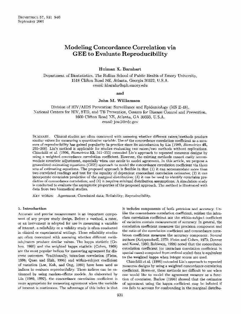
Figure 1. Systolic blood pressure data (mm Hg).

mate errors by a factor of N / ( N - 1) or even N / ( N - 2) with a small sample size.

4. Examples We illustrate the proposed method by analyzing data from two biomedical studies. The first example is from a study evaluating inexpensive electronic digital instruments (DI) for measuring blood pressure in field study settings. It is eas- ier for field personnel to use an electronic digital instrument than a mercury sphygmomanometer (MS) in measuring adult blood pressure. The original analysis for this study has been reported elsewhere using Lin’s method (Torun et al., 1998). We use this data set for illustrative purpose only. In this study, systolic and diastolic blood pressures were measured by three observers using the MS method as well as by the DI method for each subject. No covariates are available in this data set. A total of 228 adult subjects had eight readings, four for systolic blood pressure (SBP) and four for diastolic blood pressure (DBP). The ranges of SBP and DBP among the 228 subjects are 82-236 and 50-148 mm Hg, respectively.

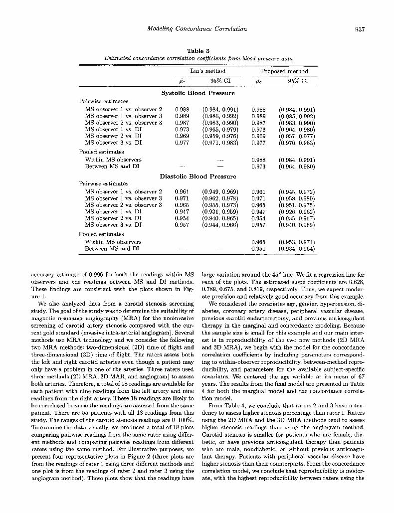
We plotted the SBP readings from MS observer i against the SBP readings from MS observer j to examine agreement within MS observers (Figure 1). We also plotted the SBP readings from MS observer 1 against the SBP readings using the DI method to explore the agreement between the MS method and the DI method (Figure 1). These plots show that the points are clustered around the 45’ line with small variation. Thus, we expect to see high precision and accuracy from these data. Plots of the DBP readings show similar findings (figure not shown). We computed all possible pairwise concordance correlation coefficients and their corresponding 95% confidence intervals (CI) using both Link method and the proposed method (Table 3).

We used indicator variables for the three observers as covariates in the marginal model for the proposed method (the DI method is treated as the reference group here). Using j = 1,2,3,4 to index the three MS readings from the three observers and one reading from the DI method, we model the concordance correlation coefficients as follows:

- - a l Z l 2 + a 2 2 1 3 + a 3 z 2 3 + a 4 z 1 4 + a 5 2 2 4 + 016234,

where Zkl(l 5 k , 1 5 4, k # 1 ) are the indicator variables for pair ( j , j ’ ) , i.e., Z k l = 1 if (Ic, l) = ( j , j ’ ) and Z k l = 0 otherwise. The above models are used to analyze the SBP and the DBP data separately. Once 15 is obtained from the third set of estimating equations, the estimated pairwise concordance correlation coefficients as well as their 95% CIS are computed using the inverse of Fisher’s 2-transformation. Note that the parameter estimates from the proposed method are identical to the ones obtained using Link method. The 95% confidence intervals using the proposed method are slightly wider than the corresponding ones using Lin’s method. This is because we use the empirically corrected standard error estimates, which do not require the normality assumption.

The estimates for the three concordance correlation coefficients within observers are similar (ranging from 0.987 to 0.989 for the SBP readings and from 0.961 to 0.971 for the DBP readings) and the estimates for the three concordance correlation coefficients between the MS and DI methods are also similar (ranging from 0.969 to 0.977 for the SBP readings and from 0.954 to 0.957 for the DBP readings). Therefore, it is useful to summarize the reproducibility by two numbers, one of which is the within-observer reproducibility and the other is the between-method reproducibility. We simplify the above model for the concordance correlation coefficients by using two parameters,

1 1 + PCZjj‘ s l o g . . . = CVlZl + a 2 z 2 ,

cv3’

where Z1 = 1 if (j,j’) equals (1,2),(1,3), or (2,3) and zero otherwise and Z 2 = 1 if (j, j’) equals (1,4), (2,4), or (3,4) and zero otherwise. The results of this simpler model are presented under pooled estimates in Table 3. The results indicate that the DI method has excellent reproducibility compared with the MS method (the concordance correlation coefficients are 0.973 with 95% CI 0.964-0.980 for SBP and 0.951 with 95% CI 0.934-0.964 for DBP) and that it is highly reproducible for observers using the MS method (the concordance correlation coefficients are 0.988 with 95% CI 0.984-0.991 for SBP and 0.965 with 95% CI 0.934-0.964 for DBP). These findings are similar to the ones reported by Torun et al. (1998).

We fit the same model using the correlation coefficient as measure of association to examine the components of precision and accuracy. For the SBP readings, we found that the correlation coefficients are 0.988 and 0.973, respectively, for the readings within MS observers and the readings between the MS and DI methods. This implies that the accuracy estimates are 1.0 and 0.996, respectively. For the DBP readings, we found that the correlation coefficients are 0.969 and 0.955, respectively, for the readings within MS observers and the readings between the MS and DI methods. This produces an


Table 3 Estimated concordance correlation coeficients from blood pressure data

Link method Proposed method

p̂ C 95% CI p̂ C 95% CI

Systolic Blood Pressure Pairwise estimates

MS observer 1 vs. observer 2 0.988 (0.984, 0.991) MS observer 1 vs. observer 3 0.989 (0.986, 0.992) MS observer 2 vs. observer 3 0.987 (0.983, 0.990) MS observer 1 vs. DI 0.973 (0.965, 0.979) MS observer 2 vs. DI 0.969 (0.959, 0.976) MS observer 3 vs. DI 0.977 (0.971, 0.983)

Within MS observers - __ Between MS and DI - -

Pooled estimates

Diastolic Blood Pressure

MS observer 1 vs. observer 2 0.961 (0.949, 0.969) MS observer 1 vs. observer 3 0.971 (0.962, 0.978) MS observer 2 vs. observer 3 0.965 (0.955, 0.973) MS observer 1 vs. DI 0.947 (0.931, 0.959) MS observer 2 vs. DI 0.954 (0.940, 0.965) MS observer 3 vs. DI 0.957 (0.944, 0.966)

Within MS observers - -

Between MS and DI -

Pairwise estimates

Pooled estimates

-

0.988 0.989 0.987 0.973 0.969 0.977

0.988 0.973

0.961 0.971 0.965 0.947 0.954 0.957

0.965 0.951

(0.984, 0.991) (0.985, 0.992) (0.983, 0.990) (0.964, 0.980) (0.957, 0.977) (0.970, 0.983)

(0.984, 0.991) (0.964, 0.980)

(0.945, 0.972) (0.958, 0.980) (0.951, 0.975) (0.926, 0.962) (0.935, 0.967) (0.940, 0.969)

(0.953, 0.974) (0.934, 0.964)

accuracy estimate of 0.996 for both the readings within MS observers and the readings between MS and DI methods. These findings are consistent with the plots shown in Fig- ure 1.

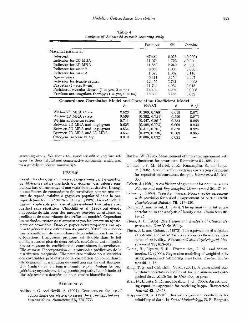
We also analyzed data from a carotid stenosis screening study. The goal of the study was to determine the suitability of magnetic resonance angiography (MRA) for the noninvasive screening of carotid artery stenosis compared with the cur- rent gold standard (invasive intra-arterial angiogram). Several methods use MRA technology and we consider the following two MRA methods: two-dimensional (2D) time of flight and three-dimensional (3D) time of flight. The raters assess both the left and right carotid arteries even though a patient may only have a problem in one of the arteries. Three raters used three methods (2D MRA, 3D MAR, and angiogram) to assess both arteries. Therefore, a total of 18 readings are available for each patient with nine readings from the left artery and nine readings from the right artery. These 18 readings are likely to be correlated because the readings are assessed from the same patient. There are 55 patients with all 18 readings from this study. The ranges of the carotid stenosis readings are &loo%. To examine the data visually, we produced a total of 18 plots comparing pairwise readings from the same rater using different methods and comparing pairwise readings from different raters using the same method. For illustrative purposes, we present four representative plots in Figure 2 (three plots are from the readings of rater 1 using three different methods and one plot is from the readings of rater 2 and rater 3 using the angiogram method). These plots show that the readings have

large variation around the 45O line. We fit a regression line for each of the plots. The estimated slope coefficients are 0.628, 0.789, 0.675, and 0.819, respectively. Thus, we expect moderate precision and relatively good accuracy from this example.

We considered the covariates age, gender, hypertension, diabetes, coronary artery disease, peripheral vascular disease, previous carotid endarterectomy, and previous anticoagulant therapy in the marginal and concordance modeling. Because the sample size is small for this example and our main interest is in reproducibility of the two new methods (2D MRA and 3D MRA), we begin with the model for the concordance correlation coefficients by including parameters corresponding to within-observer reproducibility, between-method reproducibility, and parameters for the available subject-specific covariates. We centered the age variable at its mean of 67 years. The results from the final model are presented in Table 4 for both the marginal model and the concordance correlation model.

From Table 4, we conclude that raters 2 and 3 have a ten- dency to assess higher stenosis percentage than rater 1. Raters using the 2D MRA and the 3D MRA methods tend to assess higher stenosis readings than using the angiogram method. Carotid stenosis is smaller for patients who are female, dia- betic, or have previous anticoagulant therapy than patients who are male, nondiabetic, or without previous anticoagulant therapy. Patients with peripheral vascular disease have higher stenosis than their counterparts. From the concordance correlation model, we conclude that reproducibility is moderate, with the highest reproducibility between raters using the

938 Biometrzcs, September 2001

0 2 0 4 0 a o e o

. .

0 2 0 4 o B o 8 0

Reading of observer 1 with angicgram

0 2 0 4 0 8 0 8 0

Reading of observer 1 with angicgram Reading of observer 2 with angicgram

Figure 2. Stenosis readings from the carotid screening study.

angiogram ( p c = 0.711) and the smallest reproducibility between raters using the 2D MRA method compared with raters using the angiogram (pc = 0.534). The reproducibility is higher for older patients (pvalue = 0.004 based on the Wald test for the hypothesis sage = 0). Note that the 95% confidence intervals for the concordance correlation coefficients are wide due to the small sample size and moderate precision. Furthermore, these estimates may be slightly biased down- ward based on our simulation study with small sample sizes. Therefore, we should be cautious with the interpretations of these results and one may need to confirm these results with a future reproducibility study including a larger number of patients.

We also fit the same model using the correlation coefficient as a measure of association, and the results are presented in Table 4. The estimates of p range from 0.578 (between 3D MRA and angiogram) to 0.732 (within angiogram raters). This implies that the precision of the readings is moderate. Because the correlation coefficients are not very different from the concordance correlation coefficients, we obtain high estimates for accuracy. However, the confidence intervals for accuracy estimates are wide (not shown).

5. Discussion We have proposed a GEE approach to model the concordance correlation coefficient to evaluate reproducibility. The proposed approach makes minimal distributional assumptions and takes into account the correlation between measurements made on the same subject when conducting inference. The proposed approach enables the data analyst to model differing concordance correlation coefficients simultaneously while adjusting for covariates. We illustrated the proposed method with the analyses of data from two biomedical studies.

Three sets of estimating equations may be necessary for modeling the concordance correlation coefficient. The second set of estimating equations may not be needed if moment estimates for the variances are used in place of u2 in the third set of equations. We found that the standard errors for & are not consistently estimated if only the first and the third sets of estimating equations are used because the uncertainty in estimating u2 was not taken into account. Note that the last two estimating equations may be be combined into one estimating equation by using the responses Y&yZ3,, j 5 j'. The reason that we used two sets of estimating equations is to make the distinction between the parameters u2 and a, where a ( p c ) is the main interest.

Subjects may not have an equal number of measurements in the presence of missing data. The GEE estimates may be biased if the missing data mechanism is not completely at random (Liang and Zeger, 1986). If the probability of missing is known (e.g., the missingness is by design), then one can modify the proposed GEE equations with weighted GEE equations (Robins, Rotnitzky, and Zhao, 1995). Further inves- tigation is needed if one needs to estimate the missing data mechanism.

As discussed in the Introduction, intraclass correlation (Fleiss, 1986; Quan and Shih, 1996) and within-subject coefficient of variation (Lee et al., 1989) have been used traditionally as indices to evaluate reproducibility. These indices can be estimated by using random-effects models. However, these models require full distributional assumptions. Even though these models can make covariate adjustments in the marginal mean, it is not clear how one can model the agreement measure with covariates.

As indicated by Atkinson and Nevi11 (1997), any type of correlation coefficient is highly dependent on the measurement range. Lin and Chinchilli (1997) recommended that one should always report the range of the data and judge agreement of different measurement methods over a similar ana- lytical range. These cautionary notes should be kept in mind when one uses the proposed method in practice. Also, King and Chinchilli (2000) have proposed a general index, the generalized concordance correlation coefficient, for evaluating agreement for continuous and categorical data. This index is a generalization of the concordance correlation coefficient by applying alternative functions of distance between readings other than squared distance. King and Chinchilli also in- troduced a stratified concordance correlation coefficient that adjusts for categorical covariates in the marginal mean and an extended concordance correlation coefficient that measures agreement among more than two responses.

The computer programs used in this article are available from the authors.

ACKNOWLEDGEMENTS This research was supported in part by the National Institutes of Health (NIH) grant R29 HL58014 (HXB). We would like to thank Drs Martorell and Torun (supported by the NIH grant R01 HD 29927 and the Nestle Foundation grant 573917) for providing the blood pressure data set. We also would like to thank Drs Peterman and Haber (supported by the NIH grant R01 NS 30928) for providing the data set from the carotid


Table 4 Analyses of the carotid stenosis screening study

Estimate SE P-value

Marginal parameter Intercept 47.382 6.015 <0.0001

11.074 1.723 <0.0001 Indicator for 2D MRA Indicator for 3D MRA 11.863 2.240 <0.0001 Indicator for rater 2 3.880 1.006 0.0001 Indicator for rater 3 1.679 1.067 0.116

0.411 0.154 0.007 Age in years Indicator for female gender -12.455 3.731 0.0008 Diabetes (l=yes, O=no) -11.749 4.952 0.018

14.400 4.294 0.0008 Peripheral vascular disease (1 = yes, 0 = no) Previous anticoagulant therapy (1 = yes, 0 = no) -13.305 6.188 0.032

Concordance Correlation Mode l a n d Correlation Coefficient Mode l F C 95% CI b bC.J$

Within 2D MRA raters 0.623 (0.369, 0.789) 0.639 0.971 Within 3D MRA raters 0.569 (0.302, 0.754) 0.590 0.973 Within angiogram raters 0.711 (0.447, 0.861) 0.732 0.965 Between 2D MRA and angiogram 0.625 (0.408, 0.775) 0.669 0.933 Between 3D MRA and angiogram 0.534 (0.311, 0.701) 0.578 0.924 Between 2D MRA and 3D MRA 0.567 (0.328, 0.738) 0.588 0.965 One-year increase in age 0.019 (0.006, 0.032) 0.021 - -

screening study. We thank the associate editor and two ref- erees for their helpful and constructive comments, which lead to a greatly improved manuscript.

RESUME Les ktudes cliniques sont souvent concernkes par l’kvaluation de diffhrentes raters/methods qui donnent des valeurs sem- blables lors du mesurage d’une variable quantitative. L’usage du coefficient de concordance de corrhlation comme une me- sure de reproductibilitk a gagnk en popularith dans la pra- tique depuis son introduction par Lyn (1989). La mkthode de Lin est applicable pour des ktudes kvaluant two raters /two method sans rkpktition. Chinchilli et a1 (1996) ont htendu l’approche de Lin pour des mesures rkpkthes en utilisant un coefficient de concordance de corrklation pondkrk. Cependant les mkthodes existantes n’autorisent pas facilement un ajuste- ment de covariable. Dans ce papier nous proposons une approche gknhraliske d’estimation d’kquation (GEE) pour modk- liser le coefficient de concordance de correlation via trois jeux d’hquations. L’approche proposke est flexible dans le fait qu’elle autorise plus de deux relevhs corrhlks et teste l’kgalitk des estimateurs des coefficients de concordance de corrklation. Elle autorise l’incorporation de covariables prkdictives de la distribution marginale. Elle peut 6tre utiliske pour identifier des covariables prkdictives de la corrklation de concordance; elle demande un minimum de condition sur les distributions. Une ktude de simulations est conduite pour kvaluer les pro- prihtks asymptotiques de l’approche proposke. La mkthode est illustrke avec des donnkes de deux ktudes biomkdicales.

REFERENCES Atkinson, G. and Nevill, A. (1997). Comment on the use of

concordance correlation to assess the agreement between two variables. Biometrics 53, 775-777.

Barlow, W. (1996). Measurement of interrater agreement with adjustment for covariates. Biometrics 52, 695-702.

Chinchilli, V. M., Martel, J. K., Kumanyika, S., and Lloyd, T. (1996). A weighted concordance correlation coefficient for repeated measurement designs. Biometrics 52, 341- 353.

Cohen, J. (1960). A coefficient of agreement for nominal scales. Educational and Psychological Measurement 20, 37-46.

Cohen, J. (1968). Weighted kappa: Normal scale agreement with provision for scaled disagreement or partial credit. Psychological Bulletin 70, 213-220.

Donner, A. and Koval, J. (1980). The estimation of intraclass correlation in the analysis of family data. Biometrics 36,

Fleiss, J. L. (1986). The Design and Analysis of C h i c a l Ex- periments. New York: Wiley.

Fleiss, J. L. and Cohen, J. (1973). The equivalence of weighted kappa and the intraclass correlation coefficient as measures of reliability. Educational and Psychological Mea- surement 33, 613-619.

Gonin, R., Lipsitz, S. R., Fitzmaurice, G. M., and Molen- berghs, G. (2000). Regression modeling of weighted K by using generalized estimating equations. Applied Statis-

King, T. S. and Chinchilli, V. M. (2001). A generalized concordance correlation coefficient for continuous and categorical data. Statistics in Medicine, in press.

Klar, N., Lipsitz, S. R., and Ibrahim, J. G. (2000). An estimating equations approach for modeling kappa. Biometrical Journal 42, 45-58.

Krippendorff, K. (1970). Bivariate agreement coefficients for reliability of data. In Social Methodology, B. F. Borgatta

19-25.

tics 49, 1-18.

940 Biometrics , September 2001

and G. W. Bohrnstedt (eds), 139-150. San Francisco: Jossey-Bass.

Lee, J., Koh, D., and Ong, C. N. (1989). Statistical evaluation of agreement between two methods for measuring a quantitative variable. Computers in Biology and Medicine 19, 61-70.

Liang, K. Y. and Zeger, S. L. (1986). Longitudinal data analysis using generalized linear models. Biometrika 73, 13- 22.

Liang, K. Y, Zeger, S. L., and Qaqish, B. (1992). Multivariate regression analyses for categorical data. Journal of the Royal Statistical Society, Series B 54, 3-24.

Lin, L. (1989). A concordance correlation coefficient to evaluate reproducibility. Biometrics 4 5 , 255-268.

Lin, L. (1992). Assay validation using the concordance correlation coefficient. Biometrics 48, 599-604.

Lin, L. and Chinchilli, V. (1997). Rejoinder to the letter to the editor from Atkinson and Nevill. Biometrics 53,777- 778.

Lipsitz, S. R. and Fitzmaurice, G. (1996). Estimating equations for meaures of association between repeated binary responses. Biometrics 52, 903-912.

Molenberghs, G., Fitzmaurice, G. M., and Lipsitz, S. R. (1996). Efficient estimation of the intraclass correlation for a binary trait. Journal of Agricultural, Biological, and Environmental Statistics 1 , 78-96.

Prentice, R. L. (1988). Correlated binary regression with covariates specific to each binary observation. Biometrics 44, 1033-1048.

Quan, H. and Shih, W. J. (1996). Assessing reproducibility by the within-subject coefficient of variation with random effects models. Biornetrics 52, 1195-1203.

Robieson, W. (1999). On weighted kappa and concordance correlation coefficient. Ph.D. thesis, University of Illinois in Chicago/Graduate College/Mathematics.

Robins, J. M., Rotnitzky, A., and Zhao, L. P. (1995). Analy- sis of semiparametric regression models for repeated outcomes in the presence of missing data. Journal of Amer- ican Statistical Association 90, 106-121.

Shoukri, M. M. and Mian, I. U. H. (1996). Maximum likeli- hood estimation of the kappa coefficient from bivariate logistic regression. Statistics in Medicine 15, 1409-1419.

Torun, B., Grajeda, R., Mendez, H., Flores, R., Martorell, R., and Schroeder, D. (1998). Evaluation of inexpensive digital sphygmomanometers for field studies of blood pressure. Federation of American Societies of Experimental Biology Journal 12, 5072.

Williamson, J. M., Manatunga, A. K., and Lipsitz, S. R. (2000). Modeling kappa for measuring dependent categorical agreement data. Biastatistics 1, 191-202.

Zeger, S. L. and Liang, K. Y. (1986). Longitudinal data analysis for discrete and continuous outcomes. Biornetrics 42, 121-130.

Received May 2000. Revised December 2001. Accepted December 2001.

modeling concordance correlation via gee to evaluate...

Documents