modeling compliance of the federal 1-hour no2

Modeling Compliance of The Federal 1-Hour NO2 NAAQS

CAPCOA Guidance Document

Prepared by:

CAPCOA Engineering Managers

Approved for Release October 27, 2011

CAPCOA Engineering Managers NO2 Modeling Committee

Subcommittee Members

Chris Anderson – MDAQMD Gary Arcemont – SLOCAPCD

Gerry Bemis – CEC Carol Bohnenkamp – EPA Region 9

Scott Bohning – EPA Region 9 Tom Chico – SCAQMD David Craft – MBAQMD

Ester Davila – SJVUAPCD Jorge DeGuzman – SMAQMD Ralph DeSiena – SDCAPCD

David Harris – SBCAPCD Paul Hensleigh – YSAQMD

Brian Krebs – SMAQMD Jane Lundquist – BAAQMD

Glen Long – BAAQMD Ian MacMillan – SCAQMD

Arnaud Marjollet – SJVUAPCD Kaitlin McNally – SBCAPCD Steve Moore – SDCAPCD

Wenjun Qian – CEC Glenn Reed – SJVUAPCD

Gerardo Rios – EPA Region 9 Leland Villalvazo – SJVUAPCD (Committee Chair)

Richard Wales – MDAPCD / AVAPCD Tom Weeks – SDCAPCD Gary Willey – SLOCAPCD

Preface The California Air Pollution Control Officers Association (CAPCOA) has prepared this document to provide a common platform of information, tools, and recommendations to address the new federal 1-hour NO2 National Ambient Air Quality Standard (NAAQS). The U.S. Environmental Protection Agency has provided some guidance for demonstrating through modeling that a proposed new or modified source will comply with the 1-hour nitrogen dioxide (NO2) NAAQS. That guidance is specifically for major sources and major modifications that are subject to Prevention of Significant Deterioration (PSD) requirements, and for those projects applicants should prepare protocols for the review by the appropriate agency that meet those requirements. However, agencies in California must demonstrate compliance with the 1-hour NO2 NAAQS for a variety of other regulatory programs. Existing rules may require such demonstrations for new or modified sources located in nonattainment areas. A demonstration may be necessary to satisfy the requirements of the California Environmental Quality Act (CEQA). Although federal guidance is useful for these demonstrations, such guidance is not prescriptive. The intent of this guidance document is to outline the steps necessary to demonstrate compliance with the 1-hour NO2 NAAQS. For each step, the document identifies and discusses alternative approaches that a reviewing agency can use when preparing specific guidance for projects. In addition, the document provides alternative approaches that may be incorporated into an agency’s guidance prepared specially for their jurisdiction.

Table of Contents

Glossary ........................................................................................................................... i 1 Background .............................................................................................................. 1

2 NO2 Chemistry ......................................................................................................... 2

2.1 Appendix W ....................................................................................................... 2

2.1.1 Tier 1 - Total Conversion ........................................................................... 2

2.1.2 Tier 2 - Ambient Ratio Method (ARM) ........................................................ 2

2.1.3 Tier 3 - Ozone limiting Method (OLM): ....................................................... 2

2.1.4 Tier 3 - Plume Volume Molar Ratio Method (PVMRM): ............................. 4

3 Conducting NO2 Modeling ........................................................................................ 5

3.1 What information is needed to conduct NO2 Modeling? .................................... 5

3.2 Selecting the Appropriate Model ....................................................................... 6

3.2.1 ISCST3 ...................................................................................................... 7

3.2.2 AERMOD ................................................................................................... 7

3.3 Selecting the Appropriate Tier Approach .......................................................... 7

3.3.1 Definition of Options .................................................................................. 7

3.3.2 Tier 1 - Maximum Conversion (No OLM or PVMRM) ................................. 8

3.3.3 Tier 2 - ARM (w/ Justification) .................................................................... 9

3.3.4 Tier 3 - OLM or PVMRM (w/ Justification) .................................................. 9

3.4 Other Things to Consider .................................................................................. 9

3.4.1 What is Ambient Air? ................................................................................. 9

4 NO2 Background Data ............................................................................................ 11

4.1 Maximum Hourly Concentration ...................................................................... 11

4.1.1 CARB Data .............................................................................................. 11

4.1.2 EPA’s Formatted Data ............................................................................. 11

4.1.3 EPA’s Raw Data ...................................................................................... 12

4.1.4 EPA’s AQS Web Application .................................................................... 12

4.1.5 Local Agencies ........................................................................................ 12

4.2 98th Percentile Hourly Concentration .............................................................. 12

4.2.1 CARB ....................................................................................................... 13


4.2.3 Local Agencies ........................................................................................ 13

4.3 EPA Acceptable Background Datasets ........................................................... 13

4.3.1 Monthly Hour-Of-Day ............................................................................... 13

4.3.2 Seasonal Hour-Of-Day............................................................................. 14

4.3.3 Hour-Of-Day 98th-percentile (8th Highest) value ....................................... 14

4.3.4 Missing Data (Gap Filling) ........................................................................ 15

4.3.5 Seasonal Hour-Of-Day “Winter” ............................................................... 15

5 Ozone and NO2 Datasets ....................................................................................... 16

5.1 Default Value for Missing Hourly Ozone Data (40ppb) ................................... 16

5.1.1 Default Ozone Value Determination ........................................................ 17

5.2 Are data available? ......................................................................................... 17


5.2.2 EPA’s Technology Transfer Network (TTN)/Air Quality System (AQS).... 18

5.2.3 Local Agencies ........................................................................................ 18

6 Gap Filling For Ozone and NO2 Datasets .............................................................. 19

6.1 Missing Data Procedures ................................................................................ 19

6.1.1 Single Hour .............................................................................................. 19

6.1.2 Multiple Hours .......................................................................................... 19

7 In-Stack NO2/NOX Ratio ....................................................................................... 22

7.1 Why is the NO2/NOX ratio important? .............................................................. 22

7.1.1 Conclusion ............................................................................................... 23

7.2 EPA Database ................................................................................................ 23

7.3 Manufacturer’s Dataset ................................................................................... 23

7.4 Source Testing ................................................................................................ 23

7.5 NO2/NOX Ratio Resources .............................................................................. 24

8 Demonstrating Compliance with the NAAQS ......................................................... 25

8.1 Less than Significant Impact ........................................................................... 25

8.2 Mitigation......................................................................................................... 25

8.2.1 Additional Onsite Controls ....................................................................... 25

8.2.2 On-site/Off-site Emission Reduction Credits (ERC) ................................. 25

8.3 Operating Conditions ...................................................................................... 26

8.3.1 Time of Day ............................................................................................. 26

8.3.2 Operating less than One Hour ................................................................. 26

8.4 Source Parameters ......................................................................................... 27

8.4.1 Raising Stack Height To GEP .................................................................. 27

8.4.2 Other Dispersion Techniques .................................................................. 27

8.5 Site Design ...................................................................................................... 28

8.6 Intermittent Operations ................................................................................... 28

8.6.1 Modeling Technique ................................................................................ 28

Appendix A – Modeling Procedure ................................................................................ 31

1 Introduction ............................................................................................................ 32

2 Non-Regulatory Option Checklist ........................................................................... 32

3 Model Selection Discussion and Rationale ............................................................ 32

4 Modeling Tier and Option Selection ....................................................................... 32

4.1 Tiers ................................................................................................................ 32

4.2 Tier Options .................................................................................................... 33

4.2.1 Detailed Option Descriptions ................................................................... 33

4.3 Stepwise Modeling Approach.......................................................................... 34

4.3.1 Modeling Assumptions ............................................................................. 35

4.3.2 Tier 1 – Total Conversion ......................................................................... 35

4.3.3 Tier 2 – ARM ............................................................................................ 40

4.3.4 Tier 3 – OLM/PVMRM.............................................................................. 40

4.4 Additional Guidance ........................................................................................ 41

5 Model Emission Inventory ...................................................................................... 41

5.1 Model Scenarios ............................................................................................. 42

6 Other Non-Project Sources .................................................................................... 42

7 Background Concentration ..................................................................................... 43

8 Downwash Characterization .................................................................................. 44

9 Receptor Selection ................................................................................................. 44

10 Meteorological Data ............................................................................................ 44

11 Post-Processing of the Results ........................................................................... 44

12 AERMOD Non-Regulatory Option Checklist ....................................................... 45

12.1 Source Parameter: .......................................................................................... 47

Appendix B - OLM/PVMRM Justification ....................................................................... 48

1 Background ............................................................................................................ 49

2 Non-Regulatory Option Determination ................................................................... 49

2.1 Overall Justification ......................................................................................... 50

2.1.1 Section 3.2.2 (e)(i) Requirement (Peer Review) ...................................... 50

2.1.2 Section 3.2.2 (e)(ii)Requirement (Applicable on Theoretical Basis) ......... 52

2.1.3 Section 3.2.2 (e)(iii) Requirement ............................................................ 52

2.1.4 Section 3.2.2 (e)(iv) Requirement (Performance Evaluations) ................. 53

2.1.5 Section 3.2.2 (e)(v) Requirement (Established Protocols) ....................... 54

2.2 Conclusion: ..................................................................................................... 54

Appendix C - In-Stack NO2/NOx Ratios ........................................................................ 56

Appendix D – Meteorological Resources ...................................................................... 60

1 Meteorological Resources ...................................................................................... 61

1.1 Surface Data ................................................................................................... 61

1.2 Upper Air Data ................................................................................................ 61

Page i

Glossary AERMOD AMS/EPA Regulatory Model

ARM Ambient Ratio Method

AMS American Meteorological Society

EPA Environmental Protection Agency

ERC Emission Reduction Credits

CEQA California Environmental Quality Act

CFR Code of Federal Regulations

GEP Good Engineering Practice

ISCST3 Industrial Source Complex Short-Term version 3

Monin- Obukhov Length

The Monin-Obukhov Length is a parameter with dimension of length that gives a relation between parameters characterizing dynamic, thermal, and buoyant processes. At altitudes below this length scale, shear production of turbulence kinetic energy dominates over buoyant production of turbulence.

NAAQS National Ambient Air Quality Standard

NO Nitric oxide

NO2 Nitrogen Dioxide

NOX Mono-Nitrogen Oxides (NO and NO2) or Total Oxides of Nitrogen

O3 Ozone

OLM Ozone Limiting Method

PVMRM Plume Volume Molar Ratio Method

1 Background On January 22, 2010, EPA revised the primary nitrogen dioxide (NO2) NAAQS in order to provide requisite protection of public health. Specifically, EPA established a new 1-hour standard at a level of 100 ppb (188.68 µg/m3), based on the 3-year average of the annual 98th percentile of the daily maximum 1-hour concentrations (form of the standard), in addition to the existing annual secondary standard (100 µg/m3). EPA has also established requirements for a NO2 monitoring network that will include monitors at locations where maximum NO2 concentrations are expected to occur, including within 50 meters of major roadways, as well as monitors sited to measure the area-wide NO2 concentrations that occur more broadly across communities.

The effective date of the new 1-hour standard was 60 days after the final rule was published in the Federal Register. The final rule was published in the Federal Register on February 9, 2010 with an effective date of April 12, 2010. The Federal Register Notice can be downloaded from http://www.epa.gov/ttn/naaqs/standards/nox/fr/20100209.pdf.

http://www.epa.gov/ttn/naaqs/standards/nox/fr/20100209.pdf

2 NO2 Chemistry NOx is a generic term for the total concentration of mono-nitrogen oxides, nitric oxide (NO) and nitrogen dioxide (NO2). NOx is produced from the reaction of nitrogen and oxygen gases in during combustion with air, especially at high temperatures wherein an endothermic reaction produces various oxides of nitrogen. In the ambient air, during daylight, NOX concentrations tend towards a photostationary state (equilibrium), where the ratio NO/NO2 is determined by the intensity of sunshine (which converts NO2 to NO) and the concentration of ozone and other reactive species (which react with NO to again form NO2). At night time, NO is converted to NO2 by its reaction with ozone (O3) Also, in the presence of excess molecular oxygen (O2), nitric oxide (NO) reacts with the oxygen to form nitrogen dioxide (NO2). The time required depends on the temperature and the reactant concentrations and is relatively slow in the ambient air but may be much more rapid in combustion systems. For modeling purposes, the following methods have been developed to simulate the chemical reaction of NOX to NO2 formation.

2.1 Appendix W

Appendix W of Part 51 of Title 40 of the CFR “Guideline on Air Quality Models” has codified three methods that can be used to estimate NO2 concentration (Tier 1 - Total Conversion, Tier 2 - Ambient Ratio Method or ARM, Tier 3 - Ozone Limiting Method or OLM). Please note: The Plume Volume Molar Ratio Method (PVMRM) is considered by EPA to be a Tier 3 screening method, similar to OLM.

2.1.1 Tier 1 - Total Conversion

Tier 1 - Total Conversion, assumes that the NOX emitted from a source is converted completely to NO2. No adjustment is made to consider the chemistry noted above.

2.1.2 Tier 2 - Ambient Ratio Method (ARM)

Tier 2 – ARM, the concentration from the Tier 1 analysis is multiplied by an empirically derived NO2/NOX value for the ambient air.

2.1.3 Tier 3 - Ozone limiting Method (OLM):

The following is a simplified explanation of the basic chemistry relevant to the OLM. First, the relatively high temperatures in the primary combustion zone typical of most conventional combustion sources primarily promote the formation of NO over NO2 by the following thermal reaction:

N2 + O2 ==> 2 NO NO formation in combustion zone

In lower temperature regions of the combustion zone or in the combustion exhaust, the NO that is formed can be converted to NO2 via the reaction.

2 NO + O2 ==> 2 NO2 In-stack formation of NO2

(In addition, other reactive species can convert NO to NO2 during and immediately following combustion as can oxidation catalysts in the exhaust—such as oxidation catalysts used to control carbon monoxide and volatile organic compounds.) Thus, a portion of the NOx exhausted is in the form of NO2. This is referred to as the in-stack NO2/NOx ratio, which is in general different from the ambient ratio such as that used in the ARM.

Historically, a default value of 10% of the NOx in the exhaust was assumed to be NO2. It is assumed that no further conversion by direct reaction with O2 occurs once the exhaust leaves the stack because of the much lower temperature once the exhaust mixes with the ambient air. Thus the remaining percentage of the NOx emissions is assumed to be NO.

As the exhaust leaves the stack and mixes with the ambient air, the NO reacts with ambient ozone (O3) to form NO2 and molecular oxygen (O2): NO + O3 ==> NO2 + O2 Oxidation of NO by ambient O3 The OLM assumes that at any given receptor location (ground level), the amount of NO that is converted to NO2 by this reaction is controlled by the ambient O3 concentration. If the O3 concentration is less than the NO concentration, the amount of NO2 formed by this reaction is limited. If the O3 concentration is greater than or equal to the NO concentration, all NO is assumed to be converted to NO2. In the presence of radiation from the sun, ambient NO2 can be destroyed: NO2 + sunlight ==> NO + O Photo-dissociation of NO2 As a conservative assumption, the OLM ignores this reaction. Another reaction that can form NO2 in the atmosphere is the reaction of NO with reactive hydrocarbons (HC): NO + HC ==> NO2 + HC Oxidation of NO by reactive HC The OLM also ignores this reaction.

2.1.4 Tier 3 - Plume Volume Molar Ratio Method (PVMRM):

Building on the basic OLM chemistry, the PVMRM determines the conversion rate for NOx to NO2 based on a calculation of the number of NOx moles emitted into the plume, and the number of O3 moles contained within the volume of the plume between the source and receptor. Unlike the OLM, the PVMRM method assumes an upper bound for the ambient NO2/NOx ratio. This default ambient ratio is 0.9. Please note: OLM and PVMRM are implemented as non-regulatory options in the American Meteorological Society/Environmental Protection Agency Regulatory Model (AERMOD). The Industrial Source Complex – Short-Term model (ISCST3) does not contain the PVMRM algorithms. At one time, there was a version of ISCST3 that contained the OLM algorithm. However, that particular version is not able to run on current computers. OLM can be implemented by using a post-processor program. PVMRM was initially implemented using ISCST3. But, no version of ISCST3 with the PVMRM algorithm is currently available. The dispersion algorithms in AERMOD and other steady-state plume models are based on the use of total dispersion coefficients, which are formulated to represent the time-averaged spread of the plume. A more appropriate definition of the volume of the plume for purposes of determining the number of moles of ozone available for conversion of NOx is based on the instantaneous volume of the plume, which is represented by the use of relative dispersion coefficients, (Cole and Summerhays, 1979; Bange, 1991). The implementation of PVMRM in AERMOD is based on the use of relative dispersion coefficients to calculate the plume volume. Weil (1996 and 1998) has defined formulas for relative dispersion that are consistent with the AERMOD treatment of dispersion, and which can be calculated using meteorological parameters available within AERMOD.

3 Conducting NO2 Modeling The following section only describes how and what is needed to conduct NO2 modeling. This section does not provide any details regarding the development of modeling input parameters. Please Note: Any guidance from the reviewing agency should always be followed and the information contained herein is only provided as recommendations to assist agencies in developing their own guidance.

3.1 What information is needed to conduct NO2 Modeling?

The information needed to conduct NO2 modeling will depend on the Tier and option selected to show compliance with the federal 1-hour NAAQS. Table 1 provides a quick reference of the basic information that is needed for each of the Tiers and options that are discussed in more detail in following sections. As seen in the table below each progressively refined option may require additional information and/or resources. The appropriate reviewing agency should be consulted before selecting any of the options listed in Table 1 .

Table 1- NO2 Tier Quick Reference

Tier Option Information Needed

I Total

Conversion

1 1. Model (ISCST3/AERMOD) 2. Significant Impact Level (SIL)

2 – 11 3. Background Air Quality Data

6 –11 4. Post processor*

11 5. Hourly NO2 Background Data 6. Paired-Sum Post Processor*

II ARM

1 1. Model (ISCST3/AERMOD) 2. Significant Impact Level (SIL) 3. ARM Ratio




III OLM/PVMRM

1

1. Model (ISCST3/AERMOD with a post-processor) 2. Significant Impact Level (SIL) 3. Hourly Ozone Background data 4. In-Stack NO2/NOX Ratio




*EPA’s updated AERMOD program version 11103 will support post processing and background data inputs

3.2 Selecting the Appropriate Model

Selection of the appropriate model (ISCST3/AERMOD) depends primarily on the following two items; 1) the reviewing agency’s acceptability of the model and 2) availability of appropriate meteorological data (met data). For regulatory purposes EPA’s “Preferred Model” is AERMOD. Other agencies may still be using ISCST3 as the model of choice, because most agencies in the state have or can acquire met data in ISCST3 format. Data processing requirements for AERMOD are more rigorous than for ISCST3. It may be difficult to obtain met data for some areas in the state that can be processed for use in AERMOD. A brief description and limitations of each model are provided below in order to assist agencies in determining which model should be recommended. Additionally a list of met data resources has been compiled and can be found in Appendix D.

This should assist agencies in locating the resources needed for processing AERMOD met datasets.

3.2.1 ISCST3

The ISCST3 model is based on a steady-state Gaussian plume algorithm with Pasquill-Gifford stability classes. It is applicable for estimating ambient impacts from point, area, and volume sources out to a distance of about 50 kilometers from the source. ISCST3 includes algorithms for addressing building downwash influences, dry and wet deposition, and the complex terrain screening algorithms from the COMPLEX1 model which are used to estimate concentrations for receptors that are above the top of the stack but below the plume rise. The standard version of ISCST3 is only able to perform options 1 though 5 of Tier 1 and Tier 2 of Section 3.3 without the use of a post-processor program. Therefore, its ability to conduct a more refined analysis is limited.

3.2.2 AERMOD

AERMOD is a steady-state Gaussian plume model that incorporates air dispersion based on planetary boundary layer turbulence structure and scaling concepts, including treatment of both surface and elevated sources, and both simple and complex terrain. It does not use Pasquill-Gifford stability classes. AERMOD includes algorithms for building downwash and dry and wet deposition. It includes the algorithms from the Complex Terrain Dispersion Model (CTDM) and is a refined model for intermediate and complex terrain. With the release of AERMOD (11103), it is now able to perform modeling for all Tiers in Section 3.3. This version of AERMOD has incorporated a post-processor and options for adding background data directly into the model.

3.3 Selecting the Appropriate Tier Approach

There are several options available to demonstrate compliance with the federal 1-hour NO2 standard. Not all options may be allowed by all agencies. Therefore, the reviewing agency should be consulted before applying any of the Tiers and/or options listed below.

3.3.1 Definition of Options

Significant Impact Level (SIL) is defined as a de minimis impact level below which a source is presumed not to cause or contribute to an exceedance of a NAAQS.

Maximum Modeled is defined as the maximum concentration predicted by the model at any give receptor in any given year modeled.

8th Highest Modeled is defined as the highest 8th highest concentration derived by the model at any given receptor in any given year modeled.

5yr Ave of the 98th percentile is defined as the highest of the average 8th-highest (98th percentile) concentrations derived by the model across all receptors based on the length of the meteorological data period or the X years average of 98th percentile of the annual distribution of daily maximum 1-hour concentrations across all receptors, where X is the number of years modeled. (EPA recommends in Appendix W that 5-years of meteorological data from a National Weather Service site or 1-year on-site data be modeled.)

Monthly Hour-Of-Day is defined as the 3 year average of the 1st highest concentrations (Maximum Hourly) for each hour of the day

Seasonal Hour-Of-Day is defined as the3year average of the 3rd highest concentrations for each hour of the day and season

Annual Hour-Of-Day is defined as the 3yr average of the 8th highest concentration for each hour of the day

Paired-Sum (5 yr Ave of the 98th percentile) is the merging of the modeled concentration with the monitored values paired together by month, day, and hour. The sum of the paired values are then processed to determine the X years average of 98th percentile of the annual distribution of daily maximum 1-hour concentrations across all receptors, where X is the number of years modeled.

3.3.2 Tier 1 - Maximum Conversion (No OLM or PVMRM)

1. Significant Impact Level (SIL) 2. Maximum Modeled + Maximum Monitor Value 3. Maximum Modeled + 98th Monitor Value 4. 8th Highest Modeled + Maximum Monitor Value 5. 8th Highest Modeled + 98th Monitor Value 6. 5 yr Ave of the 98th percentile + Maximum Monitor Value* 7. 5 yr Ave of the 98th percentile + 98th Monitor Value* 8. 5 yr Ave of the 98th percentile + Monthly Hour-Of-Day (1st highest)* 9. 5 yr Ave of the 98th percentile + Seasonal Hour-Of-Day (3rd Highest)* 10. 5 yr Ave of the 98th percentile + Annual Hour-Of-Day (8th Highest)* 11. Paired-Sum (5 yr Ave of the 98th percentile)** *EPA recommended option **May use with the approval of the reviewing agency.

3.3.3 Tier 2 - ARM (w/ Justification)

Please note: a value of 0.80 or 80% can be used without justifications as per EPA’s clarification memo dated March 1, 2011 (http://www.epa.gov/ttn/scram/Additional_Clarifications_AppendixW_Hourly-NO2-NAAQS_FINAL_03-01-2011.pdf) 1. Significant Impact Level (SIL) 2. Maximum Modeled + Maximum Monitor Value 3. Maximum Modeled + 98th Monitor Value 4. 8th Highest Modeled + Maximum Monitor Value 5. 8th Highest Modeled + 98th Monitor Value 6. 5 yr Ave of the 98th percentile + Maximum Monitor Value* 7. 5 yr Ave of the 98th percentile + 98th Monitor Value* 8. 5 yr Ave of the 98th percentile + Monthly Hour-Of-Day (1st highest)* 9. 5 yr Ave of the 98th percentile + Seasonal Hour-Of-Day (3rd Highest)* 10. 5 yr Ave of the 98th percentile + Annual Hour-Of-Day (8th Highest)* 11. Paired-Sum (5 yr Ave of the 98th percentile)** *EPA recommended option with justification of the ARM used **May use with the approval of the reviewing agency.

3.3.4 Tier 3 - OLM or PVMRM (w/ Justification)

1. Significant Impact Level (SIL) 2. Maximum Modeled + Maximum Monitor Value 3. Maximum Modeled + 98th Monitor Value 4. 8th Highest Modeled + Maximum Monitor Value 5. 8th Highest Modeled + 98th Monitor Value 6. 5 yr Ave of the 98th percentile + Maximum Monitor Value* 7. 5 yr Ave of the 98th percentile + 98th Monitor Value* 8. 5 yr Ave of the 98th percentile + Monthly Hour-Of-Day (1st highest)* 9. 5 yr Ave of the 98th percentile + Seasonal Hour-Of-Day (3rd Highest)* 10. 5 yr Ave of the 98th percentile + Annual Hour-Of-Day (8th Highest)* 11. Paired-Sum (5 yr Ave of the 98th percentile)** *EPA recommended option with justification of OLM or PVMRM **May use with the approval of the reviewing agency

3.4 Other Things to Consider

3.4.1 What is Ambient Air?

The following is provided to assist the reviewing agency in making a determination of their interpretation of “Ambient Air”.

3.4.1.1 Code of Federal Regulations (CFR)

40 CFR part 50.1(e) defines “Ambient Air” as meaning that portion of the atmosphere, external to buildings, to which the general public has access.

http://www.epa.gov/ttn/scram/Additional_Clarifications_AppendixW_Hourly-NO2-NAAQS_FINAL_03-01-2011.pdf


3.4.1.1.1 EPA’s Interpretation

In a letter date December 19, 1980, from Douglas Costle to Senator

Jennings Randolph, EPA further clarified this definition by stating that the

exemption from ambient air is available only for the atmosphere over land

owned and controlled by the source and to which public access is

precluded by a fence or other physical barriers.

3.4.1.1.2 Other Interpretation

As noted in the CFR notice dated February 9, 2010 entitled “Primary National Ambient Air Quality Standards for Nitrogen Dioxide”, page 6475, or 75 FR 6475 (2010-2-9), the second footnote states “The legislative history of section 109 indicates that a primary standard is to be set at ‘‘the maximum permissible ambient air level * * * which will protect the health of any [sensitive] group of the population,’’ and that for this purpose ‘‘reference should be made to a representative sample of persons comprising the sensitive group rather than to a single person in such a group.’’ S. Rep. No. 91–1196, 91st Cong., 2d Sess. 10(1970).” Taking this additional citation into consideration one could conclude that EPA’s original interpretation of ambient air is focused on a single individual and not a representative sample of persons for which the NAAQS was developed to address. Additionally, it would not be reasonable to assume that persons would be present on property owned and controlled by a source for any length of time. Therefore, it would be reasonably conservative to assume that any property owned and/or controlled, including property that is not fenced in, by a source to be exempt from ambient air as long as the appropriate and legal posting is/are provided. This posting would provide the legal means by which a source would ensure that persons would not be allowed on said property and provide the means by which said persons would be removed.

4 NO2 Background Data Based on the Tier and option selected from section 3.3 it may be necessary to calculate either the maximum 1-hour or the 3yr average of the annual 98th percentile of the maximum daily 1-hour NO2 concentration. This section provides links to online NO2 resources from EPA, CARB, and Local Agencies. To assist with the conversion of NO2 concentrations reported by the following resources the following equation is provided: NO2 Conversion (ppm to ug/m3) at Standard Temperature and Pressure

100 ug/m3

= ( 1.8868 ug/m

3

* ppb

) = 1886.8 ug/m3

53 ppb ppb 0.001 ppm ppm

4.1 Maximum Hourly Concentration

There are several online resources available for determining the maximum 1-hour NO2 concentration at a given monitoring site. These include CARB, EPA, and local agencies.

For some Tier options listed in section 3.3 the maximum 1-hour monitored concentration will be needed.

4.1.1 CARB Data

Data from CARB is located on the Air Quality Data Branch’s main webpage located at http://www.arb.ca.gov/aqmis2/aqdselect.php?tab=specialrpt. Once you navigate to the webpage follow the steps below to find the maximum 1-hour NO2 concentrations for a given monitor site.

Fill-in the information requested, except for “Step 4”. Leave “Step 4” as “Annual Statistics by Site”. Once all the information is filled in click “Retrieve Data”. Please note: you need to select Nitrogen Dioxide in “Step 1”.

4.1.2 EPA’s Formatted Data

NO2 information is also available on EPA’s AIRDATA website located at http://www.epa.gov/oar/data/geosel.html . Once you navigate to the website follow the steps below to find the maximum 1-hour NO2 concentrations for a given monitor site. Caution: data available on EPA’s site may not be as recent as that from CARB.

Step 1

Under “Select From List” header select “Select County”. Remember to also select a State. Then click “Go”.

Step 2 Select the county of interest and click the “Select County” button

http://www.arb.ca.gov/aqmis2/aqdselect.php?tab=specialrpt

http://www.epa.gov/oar/data/geosel.html

Step 3 Under Monitoring Reports click “Monitor Values”

Step 4 Under Pollutant click “NO2 – Nitrogen Dioxide” and select the year of concern. Then click the “Generate Report” Button. Please note: Additional information can be included on the report generated by selecting optional site information listed under “Optional Report Columns” header.

4.1.3 EPA’s Raw Data

EPA also provides data in raw format that can be downloaded at http://www.epa.gov/ttn/airs/airsaqs/detaildata/downloadaqsdata.htm. Please note: Files listed contain data for sites throughout the nation and can be several hundred mega bytes in size.

4.1.4 EPA’s AQS Web Application

EPA also has the Air Quality System (AQS) web application. This web application is used exclusively by Federal, State, Territorial, and Tribal environmental agencies to load and maintain air quality data. The web application can also be used to retrieve reports in formatted or raw data formats. If your agency has an AQS contact person then you can, possibly, request reports through that person. If you would like a user and password follow the instruction found at http://www.epa.gov/ttn/airs/airsaqs/registration.htm. The main AQS web application page is located at http://www.epa.gov/ttn/airs/airsaqs/aqsweb/aqswebwarning.htm.

4.1.5 Local Agencies

Local agencies typically rely on the resources provided in section 4.1.1 thru 4.1.4 to determine the maximum 1-hour concentration at a given monitor. Therefore you should contact the reviewing agency to determine which resource they would prefer, if they do not have data available.

4.2 98th Percentile Hourly Concentration

For other options listed in section 3.3 the 3yr average of the annual 98th percentile of the maximum daily 1-hour NO2 concentration will be needed. It is important to note that guidance on how to determine the 3yr average of the annual 98th percentile of the maximum daily 1-hour NO2 concentration is included in Appendix S of 40 CFR Part 50. This guidance outlines two procedures that must be performed; the highest value is determined to be the monitor’s design value (background).

http://www.epa.gov/ttn/airs/airsaqs/detaildata/downloadaqsdata.htm

http://www.epa.gov/ttn/airs/airsaqs/registration.htm

http://www.epa.gov/ttn/airs/airsaqs/aqsweb/aqswebwarning.htm

4.2.1 CARB

Currently no online NO2design value data is available from CARB.


Currently no online NO2 design values are available from EPA. In the future the AQS web application, discussed in section 4.1.4, may include a design value report that would provide the required information.


Currently some local agencies have posted the 3yr average of the annual 98th percentile of the maximum daily 1-hour NO2 concentration data either in their NO2 modeling guidance documents or on their agency’s website. Additionally, some agencies may have developed raw data processors that can process raw data available from online sources, see section 4.1.3 and 4.1.4.

4.3 EPA Acceptable Background Datasets

On March 1, 2011, EPA provided additional clarification on the implementation of the 1-Hour NO2 NAAQS; one area in which they provided guidance was on acceptable NO2 background data. The following discussion describes the options provided in the referenced memo:

Please Note: The following is only a summary of the referenced memo which provided an explanation of each the following items. The memorandum can be found at http://www.epa.gov/ttn/scram/Additional_Clarifications_AppendixW_Hourly-NO2-NAAQS_FINAL_03-01-2011.pdf.

The following three refined background datasets can be used, with the approval of the reviewing agency, and will be supported in AERMOD (11059).

Hour-Of-Day 98th-percentile (8th Highest) value

Monthly Hour-Of-Day

Seasonal Hour-Of-Day Each of the above background datasets are described below.

4.3.1 98th percentile of the Monthly Hour-Of-Day (1st Highest)

Monthly Hour-Of-Day is determined by organizing all of the NO2 concentrations by hour of day (1AM, 2AM, 3AM, etc) for each month in descending order and selecting the 1st highest NO2 concentrations (Maximum Hourly) for each hour of the day.

For example, (1AM) 1. First take all the 1AM NO2 concentrations (maximum of 28-31 numbers) for

each month



2. Organizing the NO2 concentrations in descending order (highest to lowest) 3. Take the 1st highest NO2 concentrations 4. This value will be used to represent the 1AM maximum hour or 98th-percentile

of available data 5. The above process is repeated for each hour of the day and month 6. Repeat steps 1 thru 5 for each of the three years under review 7. Average the three 1AM NO2 concentrations 8. This value will be used in AERMOD as the NO2 background concentrations

(3yr average of the 98th percentile) for the 1AM hour and month 9. Repeat step 7 and 8 for each of the hours in the day and month

4.3.2 98th percentile of the Seasonal Hour-Of-Day (3rd Highest)

Seasonal Hour-Of-Day is determined by organizing all of the NO2 concentrations by hour of day (1AM, 2AM, 3AM, etc) for each season of the year in descending order and selecting the 3rd highest NO2 concentrations for each hour of the day and season.

For example, (1AM) 1. First take all the 1AM values (maximum of 90-92 numbers) for each Season

a. Winter = December Of Previous Year, January, February b. Spring = March, April, May c. Summer = June, July, August d. Autumn = September, October, November

2. Organizing the NO2 concentrations in descending order (highest to lowest) 3. Take the 3rd highest NO2 concentrations 4. This value will be used to represent the 1AM 3rd highest or 98th- percentile of

available data 5. The above process is repeated for each hour of the day and season 6. Repeat steps 1 thru 5 for each of the three years under review 7. Average the three 1AM NO2 concentrations 8. This value will be used in AERMOD as the NO2 background concentrations

(3yr average of the 98th percentile) for the 1AM hour and season 9. Repeat step 7 and 8 for each of the hours in the day and season

4.3.3 98th percentile of The Annual Hour-Of-Day (8th Highest)

Hour-Of-Day is determined by organizing all of the NO2 concentrations by hour of day (1AM, 2AM, 3AM, etc) in descending order and selecting the 8th highest NO2 concentration for each hour of the day. This process is repeated for each of the three years under review. The procedure is similar to that used to determine a monitor’s design value (instead of daily values you use each hour of the day).

For example, (1AM) 1. First take all the 1AM NO2 concentrations (maximum of 365-366 numbers) 2. Organizing the NO2 concentrations in descending order (highest to lowest)

3. Take the 8th highest NO2 concentrations 4. This value will be used to represent the 1AM 98th- percentile of available data 5. The above process is repeated for each hour of the day 6. Repeat steps 1 thru 5 for each of the three years under review 7. Average the three 1AM NO2 concentrations 8. This value will be used in AERMOD as the NO2 background concentrations

(3yr average of the 98th percentile) for the 1AM hour 9. Repeat step 7 and 8 for each of the hours in the day

4.3.4 Missing Data (Gap Filling)

Missing Hour-Of-Day values, for the most part, are attributed to the required QA/QC and calibration requirements established by EPA and are typically scheduled during an hour(s) of low concentration. In order to ensure that all Hour-Of-Day concentrations are included the following gap filling technique is used to ensure that all Hour-Of-Day concentrations are included. Please note: EPA’s March 1, 2011 guidance document does not address missing data and therefore the following procedure is provided as an option that can be used, if required by the reviewing agency, to fill-in missing data.

4.3.4.1 Gap Filling

The same gap filling technique established by EPA for filling a single hour of missing meteorological data should be used; the missing NO2 concentration is filled using a linear interpolation using the NO2 concentration from the hour before and the hour after to replace the missing NO2 concentration.

4.3.5 Seasonal Hour-Of-Day “Winter”

To ensure consistency between the Modeled definition and the background NO2 data, the seasonal winter Hour-Of-Day values represents data from January and February of the year under review and December of the previous year. This is the definition of winter provided in the AERMOD guidance document for Seasonal Hour-Of-Day where winter is identified as including December, January, and February. It would not be appropriate to add the last month of the year, under review, to the first two months of the year.

5 Ozone and NO2 Datasets There are two main issues that need to be addressed when dealing with ozone and NO2 datasets. First, the modeling control parameter “OZONEVAL” or the default missing hourly ozone value of 40ppb. The second issue is how to deal with missing data in both the ozone and NO2 datasets. This section provides a discussion and options on how to address these issues.

5.1 Default Value for Missing Hourly Ozone Data (40ppb)

Currently there is an assumption that 40ppb is an appropriate default value for all missing ozone data. This assumption comes, in part, from an EPA addendum entitled “AERMOD: Model Formulation Document” which can be download at http://www.epa.gov/scram001/7thconf/aermod/aermod_mfd_addm_rev.pdf. Specifically, the section entitled “Minimum Ozone Concentration for Stable Concentrations” which is intended to ensure that surface measurements that may be artificially low during nighttime stable conditions due to the formation of stable vertical temperature gradient is not under estimated. This section outlines the three scenarios in which this procedure would be used in AERMOD:

0 < MOL < 50 meters (positive – very stable), then 24MAX value is substituted up to a limit of 40 ppb.

50 <= MOL <500 meters (positive - stable), then a linear interpolation is used to determine the ozone concentration (Min(40 ppb. 24MAX) * (500 - MOL)/450)

MOL => 500 meters (positive – slightly stable/neutral), then 24MAX value is substituted without limit

Where: MOL = Monin-Obukhov length 24MAX = AERMOD maximum ozone concentration over previous 24 hours

A review of the AERMOD FORTRAN source code located on EPA’s SCRAM website, specifically code file name “aermod.f” (subroutine = HRLOOP), indicates that this option is currently implemented in AERMOD.

Please Note: Since the value of 40 ppb is implemented in AERMOD and as noted above, the value was never intended to be used as a default for missing data; it is recommended that the default value of 40ppb not be used unless it has been justified and approved by the reviewing agency. Section 5.1.1 describes options on how an appropriate default value, if needed, can be developed.

http://www.epa.gov/scram001/7thconf/aermod/aermod_mfd_addm_rev.pdf

5.1.1 Default Ozone Value Determination

The purpose of a default ozone value is to take the place of any data that have been identified in an ozone file as missing (-99). Therefore, the default ozone value should be representative of the ozone data collected from the monitor to be used in the model. There are several ways that a default value can be generated. (Please note: The reviewing agency should be consulted to ensure that the selected method is appropriate.) The following are options that can be used to derive a default value in the order of conservativeness. (Note: If the ozone file has been filled in completely, every hour of the year, through gap filling then a default value does not need to be developed.) Options: 1. Maximum Annual Hourly Concentration Over the Model Period (5yrs)

Determine maximum hourly concentration for each year

Select the highest hourly concentration over the modeled period 2. Maximum Annual Hourly Concentration – For each year modeled

Determine maximum hourly concentration for each year 3. Maximum Annual Average Hourly Concentration – Over the modeling period

(5yrs)


Take the average of the maximum hourly concentration over the modeled period

4. Another option would be to use a gap filling procedure to fill-in all missing data, See Section 6 for more details.

5.2 Are data available?

There are several locations were Ozone and NO2 raw data and compiled datasets are available. EPA maintains two methods, on the web, of assessing raw air quality data from the Air Quality System (AQS) database that can be accessed depending on your agency’s affiliation. The AQS Web Application is for government agencies that maintain the monitoring sites and the TTN/AQS website which can be accessed by the general public. Additionally, some local air districts provide pre-processed Ozone and NO2 datasets that are AERMOD ready.


This web application is used exclusively by Federal, State, Territorial, and Tribal environmental agencies to load and maintain air quality data. The web application can also be used to retrieve reports in formatted (PDF) or raw data formats.

If your agency has an AQS contact person, then you can request reports through that person. If you would like a user name and password follow the instruction found at http://www.epa.gov/ttn/airs/airsaqs/registration.htm. The main AQS web application page is located at http://www.epa.gov/ttn/airs/airsaqs/aqsweb/aqswebwarning.htm.

5.2.2 EPA’s Technology Transfer Network (TTN)/Air Quality System (AQS)

EPA also provides monitoring data for download to the general public from the following web site http://www.epa.gov/ttn/airs/airsaqs/detaildata/downloadaqsdata.htm. This web site provides the same data as that of the AQS web application except that some updates may not be included in a selected file depending on the date the file was generated. Please note that the data files are for the complete national monitoring network and not by state. Therefore the file size for some datasets can be in the hundreds of megabytes. It is recommended that a post-processor be used to extract the specific data that will be used for a given project.


Local agencies have also been working on processing raw data provided by EPA or collected locally into AERMOD ready datasets. Some agencies have started posting the AERMOD ready datasets on their agency’s website. It is recommended that the reviewing agency be consulted to determine the appropriate dataset to be used.

5.2.3.1 Pre-Processor

As part of providing AERMOD ready ozone and NO2 datasets, some agencies have developed pre-processors that can be used to extract state specific data from the national data files on the Technology Transfer Network (TTN)/Air Quality System (AQS) website. The same pre-processor can generate ozone and NO2 monitoring site specific files by local air district. Below is a list of agencies that have pre-processors available:

San Joaquin Valley APCD’s pre-processor can be requested by emailing [email protected]. Additionally, the pre-processor is able to read the AMP501 report format, for ozone and NO2, generated by the AQS Web Application. This program is only for regulatory agencies.

http://www.epa.gov/ttn/airs/airsaqs/registration.htm

http://www.epa.gov/ttn/airs/airsaqs/aqsweb/aqswebwarning.htm

http://www.epa.gov/ttn/airs/airsaqs/detaildata/downloadaqsdata.htm

mailto:[email protected]

6 Gap Filling For Ozone and NO2 Datasets There are several reasons why missing data may exist in a dataset. They may be missing because of equipment malfunction, human error, or maintenance of the monitoring equipment. Nevertheless data gaps should be addressed to ensure that underestimation of NO2 impacts are minimized. The following section provides several options that may be used to fill-in data gaps. Please note: The reviewing agency should be consulted to determine the appropriate method to be used. This section only describes the method by which missing data can be filled and does not describe in any detail the procedure used to create/update ozone or NO2 files used in ISCST3 or AERMOD.

6.1 Missing Data Procedures

Several approaches may be taken when addressing missing data, but each has its own issues from being too conservative or not conservative enough. Therefore, the reviewing agency will need to determine which method is appropriate for its regulatory needs.

6.1.1 Single Hour

For a single hour, it is widely accepted that the best method of gap filling is the use of a liner interpolation of the hour before and after the missing hour. This method is also known as the mean-before-after.

Sum of the concentrations for the hour before and after

Divide the sum by 2

6.1.2 Multiple Hours

For data gaps spanning more than a single hour no single acceptable method has been developed to date. Therefore the following section will describe several methods that maybe used to fill-in gaps when more than a single hour is missing. Please note: The methods presented here are not an exhaustive list of procedures that maybe acceptable to the reviewing agency. Therefore, the reviewing agency should be consulted before processing any dataset. Note: The following methods are only intended to be used for multiple consecutive missing hours, unless otherwise noted. If only a single hour is missing it is recommended that the method described in Section 6.1.1 be used.

6.1.2.1 Simple Fill Methods

These methods are considered to be simple fill methods because they require a minimum amount of resources to be implemented and are more conservative in nature.

Gap filling Methods for Multi-hour Gaps:

1. Maximum Annual Hourly Concentration Over the Model Period (5yrs)


Select the highest hourly concentration over the modeled period

Use this value to fill-in all remaining missing hours 2. Maximum Annual Hourly Concentration – For each year modeled


Use this value to fill-in all remaining missing hours 3. Maximum Annual Average Hourly Concentration – Over the modeling

period (5yrs)


Take the average of the maximum hourly concentration over the modeled period

Use this concentration to fill-in all remaining missing hours 4. Quarterly Maximum Concentration – For each year

Determine maximum hourly concentration for each quarter (1st Qtr = Jan - March, 2nd Qtr = April – June, 3rd Qtr = July – Sept, 4th Qtr = Oct – Dec)

Use each quarter’s maximum concentration to substituted for any missing data within that quarter until all missing data is filled

5. Monthly Maximum Concentration

Determine maximum hourly concentration for each month

Use each month’s maximum concentration to fill gaps for any missing data within that month until all missing data is filled.

6.1.2.2 Complex Fill Methods

The method described in this section are considered complex in nature since they are resource intensive and may require some programming or expertise in meteorology and using spreadsheets. Additionally, this method provides a more realistic interpolation of the actual missing data because it accounts for the diurnal and seasonal change in ozone and NO2 concentration. Gap Filling Methods:

1. Monthly Hourly Concentration - Option 1 (For each year)

For each month determine the maximum concentration for each hour (1, 2, 3, …) of the day. For each month you should have 24 values.

For each missing hour within a month use the corresponding maximum hourly concentration.

Perform the above steps until all hours are filled.

Any missing hour will be filled in manually

2. Monthly Hourly Concentration - Options 2 (For each year) a. Fill any single missing hour with the maximum of the:

i. Preceding hour ii. Succeeding hour iii. Same hour of day on previous day iv. Same hour of day on succeeding day

If there is missing data for either iii and/or iv, use only the maximum of the available data to fill the missing hour (both a and b are guaranteed to be present since only single missing hours are filled in this step). Note that the most likely scenario for both c and d to be missing is for years when the monitor is calibrated at the same hour each day. In this case, the 30-day rolling average (see step b) for that hour will also not be available.

b. For hours that are not filled by step a (all periods with more than one hour missing), fill the missing hour with the maximum for that hour of day for a 30-day rolling period centered on the hour (i.e., for the 15 preceding days and the 15 succeeding days). Note that 30-day rolling period will extend into the preceding and succeeding year at the start or end, respectively, of the modeling period.

c. For hours not filled by step b, fill the missing data with the maximum of the 30-day rolling period for the preceding or succeeding hour.

d. Any hours not filled by steps a–c, are likely periods with more than a month of missing data for all hours. These will be filled on a case-by-case basis.

e. For NO2 File Only - Check all filled hours for which the filled concentration is higher than the maximum monitored concentration recorded for that day (for a complete day of missing data, the maximum monitored concentration is considered zero for purposes of this comparison). If the filled concentration is higher than the appropriate nth highest daily maximum monitored concentration for the calendar year for determining compliance with federal 1-hour standard (e.g., for 351 or more days of valid data, the 8th highest daily maximum is the appropriate value), then replace filled concentration with the appropriate nth highest daily maximum to fill that hour. Note: This prevents the filling procedure from changing the nth highest daily maximum for the year.

7 In-Stack NO2/NOX Ratio In the guidance provided by EPA the importance of in-stack NO2/NOX ratios when performing OLM or PVMRM modeling is specifically addressed. This section is intended to assist agencies in determining what in-stack NO2/NOX information is available. Data that has been gathered is provided in Appendix C.

7.1 Why is the NO2/NOX ratio important?

Equation 1 provides a basic equation that explains the importance of the in-stack NO2/NOX ratio. Equation 1: NO2 = [Ratio * (NOx)pred] + MIN [ (1-Ratio) * (NOx)pred , or (46/48) *

(O3)bkgd ]

Where: NO2 is the predicted NO2 concentration (µg/m3)

Ratio is the in-stack NO2/NOX ratio (from 0.0 thru 1.0) (NOx)pred is the model predicted NOx concentration (µg/m3) MIN means the minimum of the two quantities within the brackets (O3)bkgd is the representative ambient O3 concentration (µg/m3)

(46/48) is the molecular weight of NO2 divided by the molecular weight of O3

In Equation 1, the predicted NOx concentration is multiplied by the in-stack NO2/NOX ratio to account for the in-stack thermal conversion of NOx to NO2. The remaining NOx (assumed to be NO) is challenged by the background O3 concentration to determine the quantity of NO that is converted to NO2 in the presence of ozone.

Examples: The NOx emissions from a point source are modeled with AERMOD/ISC3 model with an in-stack NO2/NOX ratio of 0.1 (10 percent). The maximum predicted NOx concentration is 100 µg/m3. Representative ambient O3 data for the area indicate an hourly concentration of 75 µg/m3. Using Equation 1, the predicted NO2 concentration would be:

NO2 = [(0.1) * 100] + MIN [(1-0.1) * 100, or (46/48) * 75]

= 10 + MIN [90, or 72] = 82 µg/m3

This is an ozone limited case where the amount of NO2 formed is limited by the amount of O3 available.

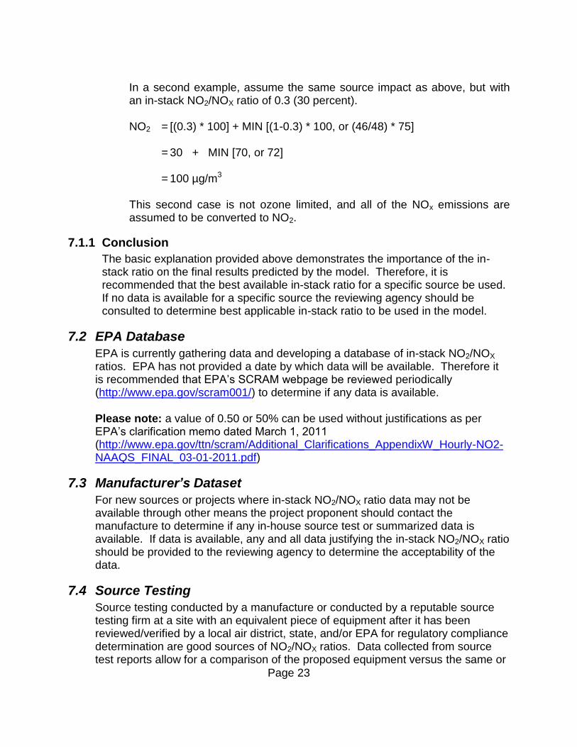
In a second example, assume the same source impact as above, but with an in-stack NO2/NOX ratio of 0.3 (30 percent).

NO2 = [(0.3) * 100] + MIN [(1-0.3) * 100, or (46/48) * 75]

= 30 + MIN [70, or 72] = 100 µg/m3

This second case is not ozone limited, and all of the NOx emissions are assumed to be converted to NO2.

7.1.1 Conclusion

The basic explanation provided above demonstrates the importance of the in-stack ratio on the final results predicted by the model. Therefore, it is recommended that the best available in-stack ratio for a specific source be used. If no data is available for a specific source the reviewing agency should be consulted to determine best applicable in-stack ratio to be used in the model.

7.2 EPA Database

EPA is currently gathering data and developing a database of in-stack NO2/NOX ratios. EPA has not provided a date by which data will be available. Therefore it is recommended that EPA’s SCRAM webpage be reviewed periodically (http://www.epa.gov/scram001/) to determine if any data is available. Please note: a value of 0.50 or 50% can be used without justifications as per EPA’s clarification memo dated March 1, 2011 (http://www.epa.gov/ttn/scram/Additional_Clarifications_AppendixW_Hourly-NO2-NAAQS_FINAL_03-01-2011.pdf)

7.3 Manufacturer’s Dataset

For new sources or projects where in-stack NO2/NOX ratio data may not be available through other means the project proponent should contact the manufacture to determine if any in-house source test or summarized data is available. If data is available, any and all data justifying the in-stack NO2/NOX ratio should be provided to the reviewing agency to determine the acceptability of the data.

7.4 Source Testing

Source testing conducted by a manufacture or conducted by a reputable source testing firm at a site with an equivalent piece of equipment after it has been reviewed/verified by a local air district, state, and/or EPA for regulatory compliance determination are good sources of NO2/NOX ratios. Data collected from source test reports allow for a comparison of the proposed equipment versus the same or

http://www.epa.gov/scram001/



similar tested equipment for the operational and control parameters implemented during the test.

7.5 NO2/NOX Ratio Resources

Currently there is no one widely accepted repository of NO2/NOX data available. As noted above, EPA is currently gathering data that will be available on their website in the near future. Other state agencies have expressed interest in gathering NO2/NOX ratio data for their own organizations, but to date no data have been published. In an effort to provide data needed for modeling and to address issues noted in EPA’s NO2 guidance memoranda, the San Joaquin Valley APCD has started gathering data from internal and external resources and has compiled NO2/NOX ratio for a variety of sources. The NO2/NOX ratios can be downloaded from http://www.valleyair.org/busind/pto/Tox_Resources/AirQualityMonitoring.htm#modeling_resources under Quick Links -Modeling Guidance- NO2/NOX In-Stack Ratios. The San Joaquin Valley APCD has also committed to update the list of ratios as new data become available. NO2/NOX ratios that have been compiled to date are also contained in Appendix C of this document. Please note: Before using any of the NO2/NOX ratio provided in Appendix C or from any other source the reviewing agency should consulted.

http://www.valleyair.org/busind/pto/Tox_Resources/AirQualityMonitoring.htm#modeling_resources

http://www.valleyair.org/busind/pto/Tox_Resources/AirQualityMonitoring.htm#modeling_resources

8 Demonstrating Compliance with the NAAQS If modeling results indicate that a project’s impact is greater than the NAAQS based on a modeled violation the options discussed below may be considered/utilized. Please note: The reviewing agency should be consulted to assist in determining the appropriate option that will be utilized to show compliance with the NAAQS.

8.1 Less than Significant Impact

If a project’s proponent can demonstrate that a project’s impact “at the point and time of any modeled violation” would not have a significant impact (less than the significant impact level or SIL) the reviewing agency can conclude that the project’s emissions would not contribute to a modeled violation and permits could be issued. This type of demonstration is only done when 1) the impacts from a project, at all locations, are less than the SIL and 2) when conducting a cumulative impact assessment. Please note: The reviewing agency should be consulted to determine the appropriate SIL to be used until such time EPA promulgates an official 1-hour NO2 SIL. (EPA has suggested using an interim value of 4 ppb, see http://www.epa.gov/nsr/documents/20100629no2guidance.pdf)

8.2 Mitigation

As noted in EPA’s memoranda, from Anna Marie Wood dated June 28, 2010 (http://www.epa.gov/nsr/documents/20100629no2guidance.pdf), there is two basic methods for mitigating modeled impacts as describe below.

8.2.1 Additional Onsite Controls

A proponent can propose additional control equipment on existing equipment at the facility to offset any modeled impact. Please note: The reviewing agency should be consulted to assist in determining the quantity of emission reductions needed to compensate for impacts of modeled violation. The reviewing agency may require that modeling be conducted to show the reduction in modeled impacts from the proposed additional controls (Impact w/o controls - Impact w/controls = Reduction in modeled impact) to demonstrate that the proposed control would reduce the modeled impact below the NAAQS or SIL.

8.2.2 On-site/Off-site Emission Reduction Credits (ERC)

The second method for mitigating a modeled violation is for a proponent to provide either on-site or off-site ERCs. When determining the quantity of ERCs needed a reviewing may consider:

http://www.epa.gov/nsr/documents/20100629no2guidance.pdf

http://www.epa.gov/nsr/documents/20100629no2guidance.pdf

Modeling procedures used to estimate impacts

NOX-NO2 conversion rates

Ambient Ozone concentrations

Other meteorological conditions in the area of concern

Therefore it is recommended that the reviewing agency be consulted in determining the appropriate quantity of ERCs needed to mitigate the modeled violation. Please note: Providing ERCs to mitigate modeled violation may not be acceptable to by all agencies. Therefore it is highly recommended that the reviewing agency be consulted.

8.3 Operating Conditions

Operating conditions can be used to demonstrate compliance with the 1-hour NAAQS. As long as those operating conditions, used to demonstrate compliance, are included as part of unit’s permit to operate issued by the reviewing agency.

8.3.1 Time of Day

“Time of day” is the concept of taking advantage of periods during the day, typically evening hours, where meteorological conditions are more favorable for dispersion and in turn reducing modeled impacts. This method is typically used by units such as emergency or back-up equipment that can be scheduled to operate only during these periods. Variable emissions or scalars can be used to adjust the operational schedule of a unit to limit its impacts. The reviewing agency may require that modeling be conducted to show the reduction from the proposed operational schedule and to demonstrate that the proposal would reduce the modeled impact below the NAAQS. Please note: The reviewing agency should be consulted to determine if this approach is appropriate.

8.3.2 Operating less than One Hour

For units that are not required to operate for a full hour they can reduce their hourly modeled impact by limiting the time they operate to less than 1-hour. For example, a unit with an hourly emissions rate of 7.0 lbs/hr of NOX can reduce its emission in half by limiting its operation to only 30 minute in any rolling hour. It is important to note that the term “in any rolling hour” is used instead of “per hour” when defining the operational limit. This term is used to ensure that the unit is not operated continuously in two different hours. For example, operating the last half of one hour and the first half of the next would result in a total of one hour of continuous operation.

In addition to establishing a condition(s) that limits the total time or time period a source would be allowed to operate, additional conditions may be needed to ensure compliance such as record keeping and/or non-resettable hour meter may be needed. Please note: The reviewing agency should be consulted to determine if this approach is appropriate.

8.4 Source Parameters

Similar to operating conditions, source parameters beyond those originally provided to the reviewing agency or those that modify standard operating parameters used to reduce modeled violations should be identified and added as a condition to permits issued by the reviewing agency. This will ensure that those assumption used are implemented and enforceable.

8.4.1 Raising Stack Height To GEP

It is widely accepted that a unit can increase its stack height to GEP as a method of reducing its modeled impacts. It must also be noted that stack height greater than GEP cannot be used when conducting modeling for demonstrating compliance with the NAAQS. Please note: If a stack height greater than GEP is proposed the reviewing agency should be consulted before being used in any modeling regiment.

8.4.2 Other Dispersion Techniques

When implementing other dispersion techniques consideration should be given to EPA’s Revised Stack Height Regulation. Guidance on the implementation of this regulation was provided by EPA in a memo dated October 10, 1985 entitled “Question and Answers on Implementing the Revised Stack Height Regulation”, see http://www.epa.gov/region7/air/nsr/nsrmemos/reinders.pdf.

8.4.2.1 Increasing Exit Velocity

For units that have low exit velocities, increasing the velocity by reducing the stack diameter or adding a blower can reduce the modeled impacts from the unit. It is important to understand that reducing a unit’s design stack diameter can cause back pressure that may affect the units operation. Therefore it is recommended that the manufacturer be consulted to determine the appropriateness of the proposed exit velocity and to ensure that any change to a unit’s stack diameter will not affect a unit’s operation. Please note: Appropriate permit conditions should be included on an agency’s permit(s) issued for a project that will ensure that the proposed unit parameters are implemented and are enforceable based on the information provided by the applicant to the reviewing agency.

http://www.epa.gov/region7/air/nsr/nsrmemos/reinders.pdf

8.5 Site Design

Another option that a proponent may implement is to redesign the facility layout / relocate equipment that is causing the modeled violation. When relocating equipment it is important to consider the following:

Distance to facility boundaries

Location to Buildings or other large airflow obstructions such as above-ground water storage tanks (Building Downwash can be a Pro or a CON)

Combined Plume Effects

Predominant hourly wind direction

Please note: If possible, this option should be implemented before any submissions to the reviewing agency are made. If this option is done during a reviewing agency’s permit review process, remodeling will be needed to demonstrate compliance with the NAAQS. Additionally, other permit conditions may be needed to ensure that proposed changes are implemented and are enforceable. Therefore, if a unit is relocated during the review process, the reviewing agency should be consulted to determine if any additional requirements will be needed.

8.6 Intermittent Operations

Intermittent operating units are those units that may or may not have a set schedule and that only operate short periods of time during the year. For example:

An emergency fire water pump driven by a diesel engine. This device must be tested for 30 minutes once per week to meet National Fire Protection Association codes.

An auxiliary generator at a power plant may operate only once per month for 60 minutes, as required by the original equipment manufacturer to ensure reliability.

This means that these units would only have an incremental impact 12 to 52 times per year. Thus, the eighth highest facility incremental impact (i.e., 98th percentile project increment) may be zero at a site with variable wind direction or very close to zero at a site with an extremely consistent wind direction.

8.6.1 Modeling Technique

On March 1, 2011 EPA provided additional clarification on intermittent operating sources that allows the reviewing agency, at their desecration, to exempt intermitted units from model requirements. The clarification memorandum can be found at http://www.epa.gov/ttn/scram/Additional_Clarifications_AppendixW_Hourly-NO2-NAAQS_FINAL_03-01-2011.pdf.



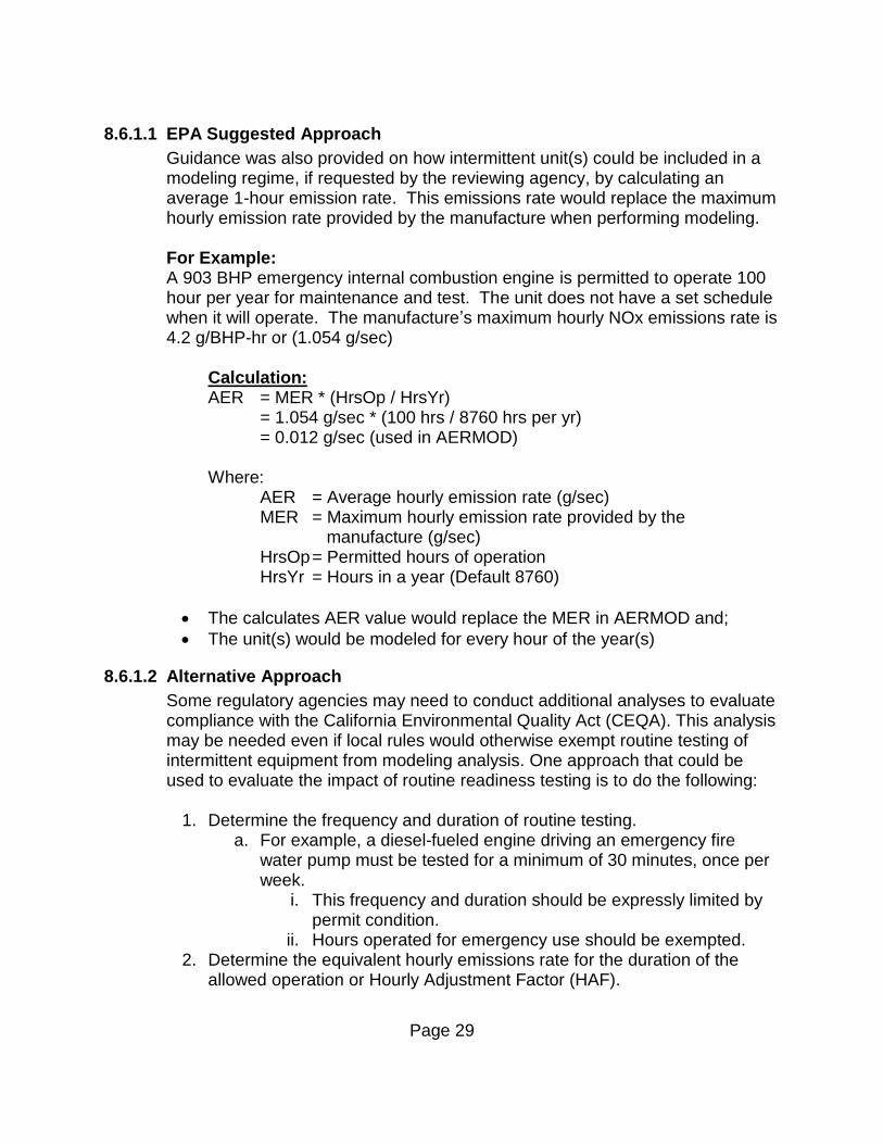
8.6.1.1 EPA Suggested Approach

Guidance was also provided on how intermittent unit(s) could be included in a modeling regime, if requested by the reviewing agency, by calculating an average 1-hour emission rate. This emissions rate would replace the maximum hourly emission rate provided by the manufacture when performing modeling.

For Example: A 903 BHP emergency internal combustion engine is permitted to operate 100 hour per year for maintenance and test. The unit does not have a set schedule when it will operate. The manufacture’s maximum hourly NOx emissions rate is 4.2 g/BHP-hr or (1.054 g/sec)

Calculation: AER = MER * (HrsOp / HrsYr) = 1.054 g/sec * (100 hrs / 8760 hrs per yr) = 0.012 g/sec (used in AERMOD) Where: AER = Average hourly emission rate (g/sec)

MER = Maximum hourly emission rate provided by the manufacture (g/sec)

HrsOp = Permitted hours of operation HrsYr = Hours in a year (Default 8760)

The calculates AER value would replace the MER in AERMOD and;

The unit(s) would be modeled for every hour of the year(s)

8.6.1.2 Alternative Approach

Some regulatory agencies may need to conduct additional analyses to evaluate compliance with the California Environmental Quality Act (CEQA). This analysis may be needed even if local rules would otherwise exempt routine testing of intermittent equipment from modeling analysis. One approach that could be used to evaluate the impact of routine readiness testing is to do the following:

1. Determine the frequency and duration of routine testing. a. For example, a diesel-fueled engine driving an emergency fire

water pump must be tested for a minimum of 30 minutes, once per week.

i. This frequency and duration should be expressly limited by permit condition.

ii. Hours operated for emergency use should be exempted. 2. Determine the equivalent hourly emissions rate for the duration of the

allowed operation or Hourly Adjustment Factor (HAF).

a. For example, if a unit operates for 30 minutes, divide the maximum hourly emissions rate by a HAF of 2

i. HAF Calculation: 60min/hr / duration of operation in minutes (min/hr).

3. Run the model with the intermittent unit modeled as "on" for each hour of each year modeled.

a. Limit emergency equipment operation to certain hours of the day for every day of the year if needed , see Step 8 below

4. Break the results for each year into periods consistent with the testing period.

a. For example, break the year into 52 weeks if the emergency equipment is only operated for routine testing once per week.

b. Retain the highest 1-hour result at each receptor location for each time period (weekly) and for each year

c. Discard any remaining values. 5. Determine the 8th highest 1-hour NO2 incremental impact at each receptor

location for each year modeled. a. At each receptor location, add this 8th highest weekly maximum

due to the intermittent unit to the 8th highest daily maximum due to the main stack(s) to calculate the cumulative project impact.

6. Compute the highest sliding 3-year average of the project’s incremental impacts at each receptor location for the years modeled.

7. Add the highest 3-year impact from step 6 to the NO2 background concentration (3yr average of the 8th highest daily maximum 1-hour NO2 monitoring concentrations).

8. If the result from Step 7 is above the federal NO2 standard due to the intermittent unit, consider limiting the allowable hours of routine readiness testing of the intermittent unit, see page 11 of EPA’s March 1, 2011 clarification memorandum (http://www.epa.gov/ttn/scram/Additional_Clarifications_AppendixW_Hourly-NO2-NAAQS_FINAL_03-01-2011.pdf)

a. For example, from 24 hours to 7 hours in a day (between the hours of 9 am to 4 pm).

b. Redo Steps 3-7. If this step is needed, write a condition imposing the allowable testing time limits.

Please Note: The responsible CEQA agency and the local reviewing agency should both be consulted to determine the appropriate approach to address intermittent unit(s).



Appendix A Page 31

Appendix A – Modeling Procedure

Appendix A Page 32

1 Introduction This modeling protocol is meant to define the stepwise approach necessary to satisfy the requirements 40 CFR 51, Appendix W section 3.2.2 (e)(v) requirements. This protocol does not override guidance provided by EPA or Appendix W of Part 51 of Title 40 of the Code of Federal Regulations.

2 Non-Regulatory Option Checklist The AERMOD Non-Regulatory Option Checklist should be completed for each project even if the ozone limiting method (OLM) or plume volume molar ratio method (PVMRM) is not used. Specific information to be provided includes the Facility Information, Project Information, Modeling Information, and Final Results. Source Parameters for all sources modeled must also be provided with the Checklist. (See Section 12)

3 Model Selection Discussion and Rationale It is recommended that the latest version of the American Meteorological Society/Environmental Protection Agency Regulatory Model or AERMOD should be used for all NO2 modeling. Use of an alternative model will require an evaluation as defined in Appendix W. Note that AERMOD is no longer a preferred model if the ambient ratio method (ARM), OLM or PVMRM are used. The use of any of these methods must be justified in accordance with the Applicability of Appendix W section 3.2.2 (e) requirements. This recommendation is based on the assumption that AERMOD ready meteorological data is available for the area under consideration. If this is not the case ISCST3 maybe used on approval from the reviewing agency.

4 Modeling Tier and Option Selection The following provides a tiered approach to analyzing compliance with the NO2 1-hour NAAQS. This tier approach is organized from the least resource intensive to most resource intensive tier and option combination. Please note: Consultation with the reviewing agency before starting a modeling analysis is highly recommended.

4.1 Tiers

Appendix W of 40 CFR 51 provides for a three tier approach for assessing compliance with the NO2 NAAQS. Each of these tiers progressively requires more detailed information to be gathered.

Tier 1 is known as “Total Conversion”. In this approach it is assumed that the amount of NOX emitted by a source or a group of sources is converted totally into NO2.

Appendix A Page 33

Tier 2 is known as the Ambient Ratio Method or ARM. In this approach an empirical ratio of NO2 to NOX is derived. This ratio is then applied to the model concentration.

Tier 3 utilizes either of two methods (OLM/PVMRM) to consider NO2 chemistry when determining the concentration at a given receptor(s).

4.2 Tier Options

Within each of the three tiers described above there are eleven options that may be applied to assess a projects compliance with the NAAQS. Each progressive option will require more information and/or resources.

Table 1 – Modeling Options

Option # Description

1 Significant Impact Level (SIL)

2 Maximum Modeled + Maximum Monitor Value

3 Maximum Modeled + 98th Monitor Value

4 8th Highest Modeled + Maximum Monitor Value

5 8th Highest Modeled + 98th Monitor Value

*6 5 yr Ave of the 98th percentile + Maximum Monitor Value

*7 5 yr Ave of the 98th percentile + 98th Monitor Value

*8 5 yr Ave of the 98th percentile + Monthly Hour-Of-Day

*9 5 yr Ave of the 98th percentile + Seasonal Hour-Of-Day

*10 5 yr Ave of the 98th percentile + Hour-Of-Day

**11 Paired-Sum (5 yr Ave of the 98th percentile)

*EPA acceptable options **May use with the approval of the reviewing agency.

4.2.1 Detailed Option Descriptions

Significant Impact Level (SIL) is defined as a de minimis impact level at which a source is presumed not to cause or contribute to an exceedance of a NAAQS.

Maximum Modeled is defined as the maximum concentration predicted by the model at any give receptor in any given year modeled.

8th Highest Modeled is defined as the highest 8th highest concentration derived by the model at any given receptor in any given year modeled.

5yr Ave of the 98th percentile is defined as the highest of the average 8th-highest (98th percentile) concentrations derived by the model across all receptors based on the length of the meteorological data period or the X years average of 98th percentile of the annual distribution of daily maximum 1-hour concentrations across all receptors, where X is the number of years

Appendix A Page 34

modeled. (EPA recommends in Appendix W that 5-years or meteorological data from a National Weather Service site or 1-year on-site data be modeled.)

Monthly Hour-Of-Day is defined as the 3 year average of the 1st highest concentrations (Maximum Hourly) for each hour of the day

Seasonal Hour-Of-Day is defined as the3year average of the 3rd highest concentrations for each hour of the day and season

Annual Hour-Of-Day is defined as the 3yr average of the 8th highest concentration for each hour of the day

Paired-Sum (5 yr Ave of the 98th percentile) is the merging of the modeled concentration with the monitored values paired together by month, day, and hour. The sum of the paired values are then processed to determine the X years average of 98th percentile of the annual distribution of daily maximum 1-hour concentrations across all receptors, where X is the number of years modeled.

4.3 Stepwise Modeling Approach

The following section provides an explanation of each of the tiers and options that can be used to comply with the NO2 standard. Table 2 below provides a quick look at the information and resources that will be needed to utilize each of the tiers and options.

Table 2- NO2 Tier Quick Reference

Tier Option Information Needed

I Total

Conversion




11 5. Hourly NO2 Data 6. Paired-Sum Post Processor*

II ARM





III OLM/PVMRM

1 1. Model (AERMOD or ISCST3 with a post-processor) 2. Significant Impact Level (SIL)

Appendix A Page 35

3. Hourly Ozone Background data 4. In-Stack NO2/NOX Ratio





4.3.1 Modeling Assumptions

The following are some basic assumptions that apply to all tiers and options, unless otherwise noted:

1 year of site specific or 5-years of NWS meteorological data will be used. Please note: A reviewing agency may approve the use of less than five years of meteorological data.

Maximum 1-hour emissions for each source will be used

4.3.2 Tier 1 – Total Conversion

Tier 1 assumes that the amount of NOX emitted by a source or group of sources is completely converted to NO2. Within Tier 1 eleven options are provided to progressively evaluate a project’s impact compared to the 1-hour NO2 NAAQS.

4.3.2.1 Option 1 – Significant Impact Level (SIL)

The maximum 1-hour concentration from any of the years modeled is compared to the interim SIL of 4 ppb. Please note: This interim SIL has not been promulgated by EPA. Therefore, agencies are allowed to develop and use their own SIL until which time EPA promulgates an official SIL.

o If the concentration is below the 1-hour NO2 SIL no further evaluation is needed.

o Else a more refined approach will be needed or; o The facility may provide the necessary quantity of mitigation to the

satisfaction of the reviewing agency.

4.3.2.2 Options 2 – Maximum Modeled + Maximum Monitor Value

The maximum 1-hour concentration from any of the years modeled is added to the maximum 1-hour monitored concentration.

The sum is then compared to the 1-hour NO2 NAAQS. o If the concentration is below the 1-hour NO2 NAAQS no further

evaluation is needed. o Else a more refined approach will be needed or; o The facility may provide the necessary quantity of mitigation to the


Appendix A Page 36

4.3.2.3 Options 3 – Maximum Modeled + 98th Monitor Value

The maximum 1-hour concentration from any of the years modeled is added to the 3yr average of the annual 98th percentile of the daily 1-hour maximum monitored concentration.




4.3.2.4 Option 4 – 8th Highest Modeled + Maximum Monitor Value

The highest 8th highest maximum 1-hour concentration from any of the years modeled is added to the maximum1-hour monitored concentration.




4.3.2.5 Options 5 – 8th Maximum Modeled + 98th Monitor Value

The highest 8th highest maximum 1-hour concentration from any of the years modeled is added to the 3yr average of the annual 98th percentile of the daily 1-hour maximum monitored concentration.




4.3.2.6 Option 6 – 5 yr Ave of the 98th percentile + Maximum Monitor

Please note: The following procedure can be used with the updated version of AERMOD 11103. AERMIOD will perform the steps listed below using the built-in post-processor.

Each year’s meteorological dataset is run independently to generate a hourly Post-Processing file:

o Unformatted (Fortran format); o Formatted Plot file – most post-processor are designed to read this

file format

Appendix A Page 37

For each year and receptor modeled, determine the maximum 1-hour concentration for each day.

For each year and receptor modeled, determine the 8th-highest daily 1-hour maximum concentration (365 or 366 values per receptor per year).

For each receptor average the 8th-highest daily 1-hour maximum concentrations across the modeled years.

The highest of the average 8th-highest1 (98th percentile) concentrations across all receptors represents the modeled 1-hour NO2 design value based on the form of the standard.

The highest 5yr average of 8th highest maximum daily 1-hour concentration is added to the maximum 1-hour monitored concentration.




4.3.2.7 Option 7 – 5yr Ave of the 98th percentile + 98th Monitor Value




file format


For each year and receptor modeled, determine the 8th-highest daily 1-hour maximum concentration (365 or 366 values per receptor per year)..

For each receptor average the 8th-highest daily 1-hour maximum concentrations across the modeled years,

The highest of the average 8th-highest (98th percentile) concentrations across all receptors represents the modeled 1-hour NO2 design value based on the form of the standard.

The highest 5yr average of 8th highest maximum daily 1-hour concentration is added to the 3yr average of the 98th percentile of the daily 1-hour maximum monitored concentration.

The sum is then compared to the 1-hour NO2 NAAQS.

1 The 8

th higest concentration is used if a full year of data are available. Otherwise, a higher rank value

must be selected.

Appendix A Page 38

o If the concentration is below the 1-hour NO2 NAAQS no further evaluation is needed.

o Else a more refined approach will be needed or; o The facility may provide the necessary quantity of mitigation to the


4.3.2.8 Option 8 – 5yr Ave of the 98th percentile + Monthly Hour-Of-Day


Five years of NCDC meteorological data is run in AERMOD or one year of onsite meteorological data

The NO2 Background option “BACKGRND” is used with the Monthly Hour-Of-Day parameter to:

o Enter each Month’s hour of the day NO2 concentrations o 24 values for each Month

Set the RECTABLE to the 8th Highest Value

Set POLLUTID to NO2

AERMOD will process each of the years and determine the 5yr average of the 8th highest maximum daily 1-hour concentration (98th percentile) which includes the NO2 background concentrations entered.

Please note: Other options are available in this version of AERMOD to determine each sources contribution to the maximum concentration noted in the AERMOD output file. Please refer to the amended AERMOD manual for more information on the use of these options (http://www.epa.gov/ttn/scram/models/aermod/aermod_userguide_addendum_v11059_draft.pdf).

4.3.2.9 Option 9 – 5yr Ave of the 98th percentile + Seasonal Hour-Of-Day



The NO2 Background option “BACKGRND” is used with the Seasonal Hour-Of-Day parameter to:

o Enter each Season’s hour of the day NO2 concentrations o 24 values for each season


Set POLLUTID to NO2


http://www.epa.gov/ttn/scram/models/aermod/aermod_userguide_addendum_v11059_draft.pdf


Appendix A Page 39

Please note: Other options are available in this version of AERMOD to determine each sources contribution to the maximum concentration noted in the AERMOD output file. Please refer to the amended AERMOD manual for more information on the use of these options (http://www.epa.gov/ttn/scram/models/aermod/aermod_userguide_addendum_v11059_draft.pdf).

4.3.2.10 Option 10 – 5yr Ave of the 98th percentile + Hour-Of-Day



The NO2 Background option “BACKGRND” is used with the Hour-Of-Day parameter to:

o Enter each hour’s NO2 concentrations o 24 values


Set POLLUTID to NO2


Please note: Other options are available in this version of AERMOD to determine each source’s contribution to the maximum concentration noted in the AERMOD output file. Please refer to the amended AERMOD manual for more information on the use of these options (http://www.epa.gov/ttn/scram/models/aermod/aermod_userguide_addendum_v11059_draft.pdf).

4.3.2.11 Option 11 – Paired-Sum (98th percentile)

Please note: The following procedure can be used with the updated version of AERMOD 11103 by including the appropriate background data. AERMIOD will perform the steps listed below using the built-in post-processor.



file format

Each year’s hourly Post-Processing file is combined temporally with the approved NO2 monitoring site’s dataset and are paired by together on a





Appendix A Page 40

monthly, daily and hourly basis to generate a new combined post-processing file (NO2 datasets must match the modeled post-processing file)


For each year and receptor modeled, determine the 8th-highest daily 1-hour maximum concentration (365 or 366 values per receptor per year).

For each receptor average the 8th-highest daily 1-hour maximum concentrations across the modeled years.

The highest of the average 8th-highest (98th percentile) concentrations across all receptors represents the modeled 1-hour NO2 design value based on the form of the standard.

The highest 5yr average of 8th highest maximum daily 1-hour concentration is then compared to the 1-hour NO2 NAAQS.

o If the concentration is below the 1-hour NO2 NAAQS no further evaluation is needed.

o Else the facility may need to provide the necessary quantity of mitigation to the satisfaction of the reviewing agency.

4.3.3 Tier 2 – ARM

Tier 2 uses an empirically derived 1-hour NO2/NOX ratio, as a method to consider the NO2 chemistry, to adjust the concentration derived by the model. There are two methods by which this can be done:

Use the maximum 1-hour NOX emissions and adjust the modeled concentration by the ARM after the model has completed or;

Adjust the maximum 1-hour NOX emissions by the ARM ratio before running the model

Please note: a value of 0.80 or 80% can be used without justifications as per EPA’s clarification memo dated March 1, 2011 (http://www.epa.gov/ttn/scram/Additional_Clarifications_AppendixW_Hourly-NO2-NAAQS_FINAL_03-01-2011.pdf)

4.3.3.1 Options 1 thru 11

The options used to conduct the modeling are the same as those in Tier 1 except as discussed above. The reviewing agency should be consulted to determine the preferred method for conduct Tier 2 modeling.

4.3.4 Tier 3 – OLM/PVMRM

Tier 3 uses non-regulatory options to further consider NO2 chemistry by using either OLM or PVMRM. Performing Tier 3 modeling will require additional resource:

AERMOD is currently the only model that incorporates both methods (OLM/PVMRM)



Appendix A Page 41

Yearly Ozone datasets – must match the years being modeled

In-Stack NO2/NOX Ratio (for each source)

4.3.4.1 Options 1 Thru 11

The options used to conduct the modeling are the same as those in Tier 1 except as discussed above. The reviewing agency should be consulted to determine the preferred ozone datasets and In-Stack NO2/NOX ratio to be used.

4.4 Additional Guidance

The use of ARM, OLM, or PVMRM must be justified using the procedures found in Appendix B. To document such approval, the AERMOD Non-Regulatory Option Checklist should be completed.

For OLM, the “OLMGROUP ALL” option should be used if there are multiple sources.

If a default ozone concentration for missing ozone data is used, the reviewing agency should be consulted to determine the appropriate method.

If version 09292 of AERMOD is used with the PVMRM option, variable emission rates should not be used. The NO2/NOX ambient equilibrium ratio for PVMRM should be provided by or approved by the reviewing agency.

5 Model Emission Inventory For sources modeled to determine compliance with the 1-hour NO2 NAAQS, the maximum 1-hour emission rates must be used unless otherwise discussed or otherwise approved by the reviewing agency. For example, an emission rate lower than the maximum 1-hour rate may be used if it will be enforceable through a permit condition. Table 8-2 in Appendix W provides specific guidance for calculating specific emission rates. The following is an extract from Table 8-2:

Appendix A Page 42

Emission Limit (lbs/MMBtu)

X Operating Level

(MMBtu/hr) X

Operating Factor (e.g., hr/yr, hr/day)

Proposed New or Modified Source

Maximum allowable emission limit or enforceable permit limit

Design capacity or enforceable permit condition

Continuous operation (i.e., all hours of each time period under consideration) for all hours of the meteorological data base

Nearby Source(s)


Actual or design capacity (whichever is greater) or enforceable permit condition


Other Source(s)


Annual level when actually operating averaged over the most recent 2 years


5.1 Model Scenarios

Note that multiple scenarios may need to be run. For example, scenarios may need to include emissions and operating conditions for 100 percent operation, 75 percent, and 50 percent. For some sources, emissions and operating conditions during normal operation, commissioning, emergency, standby, and startup or shutdown may be important as well. Please note: A reviewing agency may not require all of these scenarios to be evaluated. Consult the reviewing agency to determine which scenarios will be required.

6 Other Non-Project Sources The analysis may include sources in addition to those that are part of the project. In accordance with Appendix W, “all sources expected to cause a significant concentration gradient in the vicinity of the source or sources under consideration for emission limit(s) should be explicitly modeled.” Professional judgment should be used to identify non-project sources to be included in the analysis. The following are some examples:

1. A source with a short-stack subject to downwash is located in an area where

there are a number of other sources with short stacks subject to downwash. Unless there is another source within 100-meters, this source could be modeled alone.

Appendix A Page 43

2. A source with a relatively tall stack not subject to downwash is located in an area where there are other sources. The impact area (i.e., the area in which the source will have an impact equal to the SIL) should be determined. Other sources that are within that impact area should be included in the analysis. Consideration of Appendix W’s guidance regarding the concentration gradient should be given to selecting sources to model.

7 Background Concentration All ambient air quality analyses that are intended to determine the total pollutant concentration for comparison with the standard will include explicit modeling of the project sources and may include other non-project sources as discussed above. In addition, a background concentration must be included that represents the contribution from sources that are not modeled.

The most recent air quality design value (i.e., the three-year average of the 98th percentile of the daily maximum 1-hour concentrations) of a representative monitoring site should be used for the background concentration. The representativeness of the monitoring site will depend upon the following factors:

1. Proximity to the source(s) being modeled. In general, the nearest monitoring site

is preferable. 2. Similarity of surrounding source(s). Sources in the vicinity of the monitor should

be similar to those near the source(s) modeled. 3. Conservativeness of the background concentrations. The intent of any analysis

is to ensure that it is “conservative” (i.e., ambient concentrations are overestimated). Thus, an effort should be made to select a background monitoring site where the measured concentrations are equal to or greater than those that would be measured were a monitor to be located in the vicinity of the source(s) to be modeled.

4. Another issue that must be considered is the contribution by sources in the vicinity of the background monitor to concentrations at the monitor. Because many existing monitors are located in urban and suburban areas, numerous small sources in the vicinity of the monitor may be contributing to the concentrations measured at the monitor. The analysis of a source that is located in a similar area would not need to include these additional sources. But, the analysis of a source located in a remote area using background data from a monitor that is not affected by sources surrounding the project may need to include these additional sources to ensure that proper consideration is given.

5. Selection of the background monitoring site and the factors that led to its selection should be documented.

Please note: The reviewing agency should be consulted to determine the appropriateness of a selected monitoring site.

Appendix A Page 44

8 Downwash Characterization Care should be exercised to ensure that downwash is properly considered. When there is reason to believe that inclusion of downwash in the analysis will result in a higher estimate of pollutant concentrations, downwash should be included. Otherwise, the analysis can proceed without downwash.

9 Receptor Selection Receptors should be selected to ensure that the maximum concentration is predicted. It may be necessary to model a nested refined grid if the original coarser grid does not identify the maximum concentration.

10 Meteorological Data The meteorological data used in an analysis should be representative of the area in which the source(s) is located. To determine representativeness, consideration should be given to the land uses in the vicinity of the meteorological site versus that near the source(s). For example, it may be appropriate to use a site located further away versus an urban site that is located nearer to a project located in a rural area.

10.1 Gap Filling

If missing meteorological data is to be filled, the reviewing agency should be consulted to ensure the appropriate fill method is utilized. At a minimum the procedures outline by EPA should be reviewed (http://www.epa.gov/ttn/scram/surface/missdata.txt).

11 Post-Processing of the Results As discussed above, some analytical tiers may require the use of a post-processor. Some agencies have developed interim post-processor for use with AERMOD. AERMOD version 11103 has been enhance to incorporate a post-processor and should be used unless otherwise instructed by the reviewing agency.

http://www.epa.gov/ttn/scram/surface/missdata.txt

Appendix A Page 45

12 AERMOD Non-Regulatory Option Checklist Approved Site Specific Parameters

Items that are required for a Case – By – Case determination are noted with an *

Facility Information

Facility ID

Name

Address

City/State

Comments

Project Information

Facility ID

Project ID

Description

Comments

Modeling Information*

Model EPA AERMOD Version (XXXXX)

Operating Scenario

Normal or Commissioning or Emergency or Standby

Met Data

Site Name

Years Start: End:

Type NWS or MM5

Terrain Flat or Elevated:

Site Location Zone: UTME: UTMN:

Ozone Limiting ARM or OLM or PVMRM

Source Parameter See Tables Below

Background Site

Name

Location Zone: UTME: UTMN:

Years Start: End:

Location Type Urban or Rural

Distance From Project (km)

Comments

Appendix A Page 46

Final Results*

Averaging Period/Concentration (Background + Model)

Comments Tier Option Information Needed

I Total

Conversion





II ARM





III OLM/PVMRM

1

1. Model (ISCST3/AERMOD with a post-processor) 2. Significant Impact Level (SIL) 3. Hourly Ozone Background data 4. In-Stack NO2/NOX Ratio





Conclusion* It has been determined that enough information has been provided to conclude that OLM or PVMRM are appropriate for the above modeling scenario.

Supervisor Name

Supervisor Signature

Comments

Appendix A Page 47

12.1 Source Parameter:

The following information should be provided for each different source that is modeled.

Source Parameters For (Unit ID or Description)

Source Type Point Location Type Urban/Rural

Stack Height (m) Max Hours per Year

Stack Diameter. (m) Fuel Type

Stack Exit Velocity (m/s) NO2/NOx Ratio (%) /

Stack Exit Temp. (°K)

Rating (MMBtu/hr)

Appendix B Page 48

Appendix B - OLM/PVMRM Justification

Appendix B Page 49

1 Background In June of 2010, EPA issued two clarification memoranda concerning the implementation of the federal 1-Hour NO2 standard as it relates to PSD permitting. These memoranda provided guidance on the use of AERMOD as it relates to modeling options and requirements for using alternative models/non-regulatory options. In brief, the use of non-regulatory options in AERMOD, specifically the Ozone Limiting Method (OLM) and the Plume Volume Molar Ratio Method (PVMRM), would change the status of the model as stated in Section 3.1.2(c) of 40 CFR Part 51, Appendix W,”A preferred model should be operated with the options listed in Appendix A as ‘‘Recommendations for Regulatory Use.’’ If other options are exercised, the model is no longer ‘‘preferred.’’ Any other modification to a preferred model that would result in a change in the concentration estimates likewise alters its status as a preferred model. Use of the model must then be justified on a case-by-case basis.” In order for non-regulatory options to be used for regulatory purposes the following determination must be made as per section 3.2.2 (e) “… an alternative refined model may be used provided that:”

i. The model has received a scientific peer review; ii. The model can be demonstrated to be applicable to the problem on a theoretical basis; iii. The databases which are necessary to perform the analysis are available and adequate; iv. Appropriate performance evaluations of the model have shown that the model is not biased toward underestimates; and v. A protocol on methods and procedures to be followed has been established.”

2 Non-Regulatory Option Determination A reviewing agency may approve the use of a refined alternative model as long as the five items in section 3.2.2 (e) of 40 CFR Part 51, Appendix W have been addressed to the satisfaction of the reviewing agency. This determination must be done on a case-by-case basis. In order to facilitate this process the following framework will be used to justify those issues that are consistent from one project to another. This will allow for a streamline review of the critical modeling inputs that are unique to each project. The following approach will justify the use of OLM/PVMRM for projects 1) an overall justification will be provided to address each of the five requirements listed in section 3.2.2 (e) and 2) each project will be required to complete a questionnaire

Appendix B Page 50

intended to provide project specific information that will allow for a streamline determination of the appropriateness of the non-regulatory option(s) used (OLM/PVMRM) on a case-by-case basis, see Appendix A, Section 12.

2.1 Overall Justification

The following will address each of the five requirements noted in 3.2.2.(e) in order to justify the use of OLM/PVMRM for the purpose of determining compliance with the federal 1-hour NO2 standard.

2.1.1 Section 3.2.2 (e)(i) Requirement (Peer Review)

The requirement of section 3.2.2 (e)(i) is:

Has the model received a scientific peer review? As noted in the memorandum from Taylor Fox on June 28, 2010; “Since AERMOD is the preferred model for dispersion for a wide range of application, the focus of the alternative model demonstration for use of the OLM/PVMRM options within AERMOD is on the treatment of NOX chemistry within the model, and does not need to address basic dispersion algorithms within AERMOD.” Therefore the following will address the basic chemistry of each of the non-regulatory options.

2.1.1.1 Basic OLM Chemistry:

To provide some background, the following is a simplified explanation of the basic chemistry relevant to the OLM. First, the relatively high temperatures typical of

most combustion sources promote the formation of NO2 by the following thermal reaction: 2 NO + O2 ==> 2 NO2 In-stack formation of NO2 OLM assumes a default 10% of the NOx in the exhaust is converted to NO2 by this reaction, and no further conversion by this reaction occurs once the exhaust leaves the stack. Please Note: The District has compiled a list of NO2/NOx ratios that can be used as default in-stack NO2/NOx ratios until source test data become available, see Table 1. The remaining percentage of the NOx emissions is assumed to be nitric oxide (NO). As the exhaust leaves the stack and mixes with the ambient air, the NO reacts with ambient ozone (O3) to form NO2 and molecular oxygen (O2): NO + O3 ==> NO2 + O2 Oxidation of NO by ambient O3 The OLM assumes that at any given receptor location, the amount of NO that is converted to NO2 by this reaction is proportional to the ambient O3 concentration. If the O3 concentration is less than the NO concentration, the amount of NO2 formed by this reaction is limited. If the O3 concentration is greater than or equal to the NO concentration, all of the NO is assumed to be converted to NO2.

Appendix B Page 51

In the presence of radiation from the sun, ambient NO2 can be destroyed: NO2 + sunlight ==> NO + O Photo-dissociation of NO2 As a conservative assumption, the OLM ignores this reaction. Another reaction that can form NO2 in the atmosphere is the reaction of NO with reactive hydrocarbons (HC): NO + HC ==> NO2 + HC Oxidation of NO by reactive HC The OLM also ignores this reaction. This may be a non-conservative assumption with respect to NO2 formation in urban/industrial areas with relatively large amounts of reactive HC emissions.

2.1.1.2 Basic PVMRM Chemistry:

Building on the basic OLM chemistry, the PVMRM determines the conversion rate for NOx to NO2 based on a calculation of the NOx moles emitted into the plume, and the amount of O3 moles contained within the volume of the plume between the source and receptor. Please note: OLM and PVMRM are implemented as non-regulatory options in the American Meteorological Society/Environmental Protection Agency Regulatory Model (AERMOD). The Industrial Source Complex – Short-Term model (ISCST3) does not contain the PVMRM algorithms. At one time, there was a version of ISCST3 that contained the OLM algorithm. However, that particular version is not able to run on current computers. OLM can be implemented by using a post-processor program. PVMRM was initially implemented using ISCST3. But, no version of ISCST3 with the PVMRM algorithm is currently available. The dispersion algorithms in AERMOD and other steady-state plume models are based on the use of total dispersion coefficients, which are formulated to represent the time-averaged spread of the plume. A more appropriate definition of the volume of the plume for purposes of determining the ozone moles available for conversion of NOx is based on the instantaneous volume of the plume, which is represented by the use of relative dispersion coefficients, (Cole and Summerhays, 1979; Bange, 1991). The implementation of PVMRM in AERMOD is based on the use of relative dispersion coefficients to calculate the plume volume. Weil (1996 and 1998) has defined formulas for relative dispersion that are consistent with the AERMOD treatment of dispersion, and which can be calculated using meteorological parameters available within AERMOD.

Appendix B Page 52

The chemistry for both models has been peer-reviewed as noted by the documents posted on EPA’s Support Center for Regulatory Air Modeling (SCRAM) web site entitled “Sensitivity Analysis Of PVMRM And OLM In AERMOD” and “Evaluation Of Bias In AERMOD-PVMRM”. Both documents indicate that the models appear to perform as expected.

2.1.2 Section 3.2.2 (e)(ii)Requirement (Applicable on Theoretical Basis)

The requirement of 3.2.2 (e)(ii) is:

Can the model (OLM or PVMRM) be demonstrated to be applicable to the problem on a theoretical basis?

As noted in the document entitled “Sensitivity Analysis of PVMRM and OLM In AERMOD” prepared by Roger W. Brode of MACTEC Federal Programs, Inc., (Now with EPA’s Office of Air Quality Planning and Standards or OAQPS) “This report presents results of a sensitivity analysis of the PVMRM and OLM options for NOx to NO2 conversion in the AERMOD dispersion model. Several single source scenarios were examined as well as a multiple-source scenario. The average conversion ratios of NO2/NOx for the PVMRM option tend to be lower than for the OLM option and for the Tier 2 option or the Ambient Ratio Method which has a default value of 0.75 for the annual average. The sensitivity of the PVMRM and OLM options to emission rate, source parameters and modeling options appear to be reasonable and are as expected based on the formulations of the two methods. For a given NOx emission rate and ambient ozone concentration, the NO2/NOx conversion ratio for PVMRM is primarily controlled by the volume of the plume, whereas the conversion ratio for OLM is primarily controlled by the ground-level NOx concentration.

Overall the PVMRM option appears to provide a more realistic treatment of the conversion of NOx to NO2 as a function of distance downwind from the source than OLM or the other NO2 screening options (Hanrahan, 1999a; Hanrahan, 1999b). No anomalous behavior of the PVMRM or OLM options was identified as a result of these sensitivity tests.” Based on this report for both OLM/PVMRM appear to be applicable to the problem of NO2 formation and as noted by the author provides a better estimation of the NO2 impacts compared to other screening options (Tier 1 and 2).

2.1.3 Section 3.2.2 (e)(iii) Requirement

The requirement of 3.2.2 (e)(iii) is:

The databases which are necessary to perform the analysis are available and adequate.

The data needed to conduct an OLM/PVMRM run are:

Appendix B Page 53

Hourly meteorological data,

Hourly ozone data, and

In-stack NO2/NOx ratio

2.1.3.1 Meteorological and Ozone Datasets (Availability of Databases)

Meteorological and ozone datasets used for perform modeling runs should be processed using applicable EPA guidance. Guidance for filling in missing meteorological data entitled “Missing Data Procedures for Substituting Values for Missing NWS Meteorological Data for Use in Regulatory Air Quality Models” can be found at http://www.epa.gov/ttn/scram/surface/missdata.txt. Currently no guidance is available from EPA on filling in missing ozone data. Section 7.0 of the main document provides a suggested method for filling in missing ozone data that may be used upon approval of the reviewing agency.

2.1.3.2 In-Stack NO2/NOX Ratio

Currently, limited information is available on in-stack NO2/NOx ratios nation-wide. A literature search of available data revealed in-stack NO2/NOx ratios for a limited number of sources, see Appendix C. If a source is not listed, the source type that best represents the source under review should be used. In addition EPA and some local air district have started collecting in-stack NO2/NOx data that is obtained during annual source testing, if available. These data are being compiled, and new In-stack NO2/NOx ratios and source categories are being developed.

2.1.4 Section 3.2.2 (e)(iv) Requirement (Performance Evaluations)

The requirement of 3.2.2 (e)(iv) is:

Has an appropriate performance evaluations of the model (OLM/PVMRM) shown that the model is not biased toward underestimates?

As noted in the document entitled “Evaluation Of Bias In AERMOD-PVMRM” prepared by Roger W. Brode of MACTEC Federal Programs, Inc.,(Now with EPA OAQPS) “This report presents results of an analysis of evaluation results to determine whether the AERMOD-PVMRM algorithm produces biased or unbiased estimates of the NO2/NOx ratio. Evaluation results from two aircraft studies and two long-term field studies were examined, as well as comparisons between AERMOD-PVMRM and other refined chemically reactive plume models. Comparisons between predicted and observed NO2/NOx ratios were based on results paired in time and space, providing a more rigorous assessment than is commonly used in evaluating the performance of air dispersion models. While there does not appear to be a clear and objective criterion established by EPA for determining whether a model is biased or unbiased, a general “rule of thumb” that is commonly used as a benchmark in judging the performance of air dispersion models is agreement with observations within a factor of two.

http://www.epa.gov/ttn/scram/surface/missdata.txt

Appendix B Page 54

…In all cases, the average ratio between predicted and observed NO2/NOx ratios showed agreement within a factor of two, and in most cases within about a factor of 1.5. Based on all of the data available, the AERMOD-PVMRM algorithm is judged to provide unbiased estimates of the NO2/NOx ratio based on criteria that are comparable to, or more rigorous than, evaluations performed for other dispersion models that are judged to be refined, implying unbiased performance.” As noted in the above report it has been determined that PVMRM has been judged to provide unbiased estimates based on criteria that are comparable to, or more rigorous than, evaluations performed for other dispersion models. At the present time no assessment of bias has been conducted for the OLM algorithm. It has been shown in the sensitivity analysis, see discussion on section 3.2.2 (e)(ii) above, that OLM provides similar more conservative results than PVMRM. Therefore is it assumed that OLM would also provide an unbiased estimate of the modeled concentration.

2.1.5 Section 3.2.2 (e)(v) Requirement (Established Protocols)

The requirement of 3.2.2 (e)(iv) is:

Has a protocol on methods and procedures to be followed been established?

The methods and procedures outlined in Appendix A which is entitled “Modeling Procedures” will be implemented to comply with this requirement.

2.2 Conclusion:

Based on the information provided in section 2.1.1 thru 2.1.5, it has been shown that the method for determining hourly NO2 concentrations using AERMOD in conjunction with the non-regulatory OLM or PVMRM options is an acceptable option based on the requirements of 40 CFR Part 51, Appendix W, 3.2.2(e), see below.

Section 3.2.2 (e)(i). The model has received a scientific peer review;

The chemistry for both models has received scientific peer review as noted in “Sensitivity Analysis of PVMRM and OLM in AERMOD” and “Evaluation of Bias in AERMOD-PVMRM”. Both documents indicate that the models appear to perform as expected

Section 3.2.2 (e)(ii). The model can be demonstrated to be applicable to the problem on a theoretical basis;

Both models have been reviewed and the chemistry has been widely accepted by EPA and other government agencies as being appropriate for addressing the formation of NO2 and the calculation of NO2

Appendix B Page 55

concentration at receptors downwind. Additionally, the ““Sensitivity Analysis of PVMRM and OLM in AERMOD” report would indicate OLM/PVMRM provides a better estimation of the NO2 impacts compared to other screening options.

Section 3.2.2 (e)(iii). The databases which are necessary to perform the analysis are available and adequate;

The District will process both the meteorological and ozone data using applicable guidance and procedure. Additionally, the District will continue to gather/develop NO2 ratios as needed.

Section 3.2.2 (e)(iv). Appropriate performance evaluations of the model have shown that the model is not biased toward underestimates;

As noted the “Evaluation of Bias In AERMOD-PVMRM” report, PVMRM has been judged to provide an unbiased estimate. Based on the sensitivity study, OLM was estimated to provide similar or more conservative estimates of concentration than PVMRM and therefore would also be judged to be unbiased to underestimation.

Section 3.2.2 (e)(v). A protocol on methods and procedures to be followed has been established.”

The methods and procedures for conducting an assessment for determining compliance with the federal 1-hour NAAQS are contained in Appendix A of this document

.

Appendix C Page 56

Appendix C - In-Stack NO2/NOx Ratios

Appendix C Page 57

Recommend In-stack NO2/NOx Ratios

Refer #

Fuel Equipment Category (Controls) Range of Ratios (%) Recommended Ratio (%)

Boilers

1

NG

Default 10 10

2 6.6 MMBtu/Hr (Force Draft)*L 0.0 – 2.90 1.58**

2 7.6 MMBtu/Hr (SCR / FGR)* 3.45 – 15.79 9.65**

2 11.4 MMBtu/Hr (Force Draft)*L 1.81 – 3.51 2.68**

Compressor IC Engines

1

NG

Default 60 60

2a 225 BHP IGN Timing BTC 17*** 11.61 – 11.86 11.76**









2a 1500 BHP IGN Timing BTC 6.5*** 18.42 – 21.33 19.97**


2a Waste Gas (Field Gas)

880 BHP IGN Timing BTC 20*** 1.77 – 6.10 3.86**

2a 1000 BHP*** 0.40 – 0.81 0.64**

Dryer

NG 20 MMBTU/Hr (Milk -Tower Dryer)* 3.85 – 11.11 6.88**

Glass Furnace

2 NG Glass Furnace 2.45 – 11.59 4.32**

Heaters

2 NG / Refinery Gas

14.1 MMBTU/Hr (John Zink PSMR)* 11.54 – 52.63 32.0**

Appendix C Page 58


Refer #


IC Engines

2 Biogas 200 BHP* 0.0 – 1.90 0.37**

1 Diesel

Default 20 20

322 BHP (WP)* 0.0 – 50.0 15.64**

4

NG

Default – Lean Burn 5-10 10

2 120 BHP (3-Way Catalyst)* 0.1 – 2.83 0.9**

2 162 BHP (catalytic converter, air/fuel ratio)* 0.0 – 12.5 1.81**

2 165 BHP (3-Way Catalyst)* 0.0 – 17.58 3.16**

2 180 BHP (NSCR)* 1.02 – 3.41 1.82**

2 208 BHP (catalytic converter, air/fuel ratio)* 0.0 – 1.44 0.48**

2 1,070 BHP (LB/WP–Turbocharger/Intercooler)* 20.91 – 39.62 34.41**

2 1,529 BHP (LB - CO Catalyst, SCR)* 2.70 – 4.58 3.59**

2 2,775 BHP (SCR)* 14.53 – 26.33 19.46**

2 4,175 BHP (SCR,CO & VOC Catalysts)* 0.0 – 21.28 1.15**

Transportation Refrigeration Units (TRUs)

5

Fuel Eng Speed

Exhaust NO2/ NOx Ratio

CARB High Muffler 15.37

CARB= CARB Diesel GTL High Muffler 16.17

GTL = Gas To Liquid CARB High pDPF 25.71

CARB Low Muffler 22.66

GTL Low Muffler 25.12

CARB Low pDPF 12.98

Truck / Cars

6 Gas/Diesel Light / Medium Duty 16-25 25

Diesel Heavy Duty 6-11 11

Turbines

3 NG GE Turbines 8.33 – 9.1 9.1

Appendix C Page 59


Refer #


2a Solar Centaur T-4702 (3.4 MW)*** 8.43 – 12.42 10.32**

* Samples taken each minute or several minutes

**Value represents the statistical average of all data points *** 30 min / 1 hour Source Test

L = Load ratings have been included in average

LB = Lean Burn

WP = Water Pump

References

1. Barrie Lawrence, Environmental Scientist, Government of Newfoundland and Labrador, “Guideline for Plume Dispersion Modeling” 1st Revision: November 20, 2006, Page 14

2. District Database “NO2 -NOx Ratio.mdb” - Data is based on CEMs, source test, and portable analyzer data collected in the San Joaquin Valley

a. District Database “NO2 -NOx Ratio.mdb” - Data is based on source test data collected from out of state (Arkansas Department of Environmental Quality Office of Air Quality)

3. Roointon Pavri and Gerald D. Moore, GE Energy Services Atlanta, GA, “Gas Turbine Emissions and Control” March 2001 Page 63

4. Nigel N. Clark, Center for Alternative Fuels, Engines and Emissions Department of Mechanical and Aerospace Engineering West Virginia University Morgantown, WV 26506, “Selective NOx Recirculation for Stationary Lean-Burn Natural Gas Engines” April 30, 2007 Page 64

5. Robb A. Barnitt, National Renewable Energy Laboratory, “Emissions of Transport Refrigeration Units with CARB Diesel, Gas-to-Liquid Diesel, and Emissions Control Devices”, May 1, 2010

6. P G Boulter, I S McCrae, and J Green, Transportation research Laboratory, “Primary NIO2 Emissions From Road Vehicles in the Hatfield and Bell Commons Tunnels”, July 2007

Appendix D Page 60

Appendix D – Meteorological Resources

Appendix D Page 61

1 Meteorological Resources

1.1 Surface Data

Several online resources are available for acquiring and processing raw met data. The EPA’s SCRAM website located at (http://www.epa.gov/ttn/scram/metobsdata_databases.htm) has formatted and raw met data for some locations within California for both ISCST3 and AERMOD. Data available for AERMOD must still be processed using the AERMET program. Guidance on how to download raw data from the NCDC website and general processing techniques can be downloaded from the San Joaquin Valley APCD at http://valleyair.org/busind/pto/Tox_Resources/AirQualityMonitoring.htm#modeling_guidance. The document entitled “District Meteorological Processing Procedures” provides a step by step procedure for acquiring and processing raw NCDC data. The second is a zip file entitled “Meteorological Data Template” that provides templates for the raw data from NCDC and the NCDC_CNV program that will convert raw NCDC data in a SAMSON format that AERMET can read. The conversion program was developed and distributed without charge by Russell F. Lee of RF Lee Consulting, Charlotte, NC.

1.2 Upper Air Data

Upper Air Data can be downloaded free of charge from http://esrl.noaa.gov/raobs/.

http://www.epa.gov/ttn/scram/metobsdata_databases.htm

http://valleyair.org/busind/pto/Tox_Resources/AirQualityMonitoring.htm%23modeling_guidance

http://valleyair.org/busind/pto/Tox_Resources/AirQualityMonitoring.htm%23modeling_guidance

http://esrl.noaa.gov/raobs/

modeling compliance of the federal 1-hour no2

Documents