modeling and solving vehicle routing problems with many ... · by using a standard set of test...
TRANSCRIPT

MASTER’S THESIS
Department of Mathematical Sciences Division of Mathematics CHALMERS UNIVERSITY OF TECHNOLOGY UNIVERSITY OF GOTHENBURG Gothenburg, Sweden 2014
Modeling and solving vehicle routing problems with many available vehicle types
SANDRA ERIKSSON BARMAN

Thesis for the Degree of Master of Science
Department of Mathematical Sciences Division of Mathematics
Chalmers University of Technology and University of Gothenburg SE – 412 96 Gothenburg, Sweden
Gothenburg, May 2014
Modeling and solving vehicle routing problems with many available vehicle types
Sandra Eriksson Barman

�
Matematiska vetenskaper Göteborg 2014
Abstract
In this thesis, models have been formulated and mathematical optimiza-tion methods developed for the heterogeneous vehicle routing problemwith a very large set of available vehicle types, called many-hVRP. Thisis an extension of the standard heterogeneous vehicle routing problem(hVRP), in which typically fairly small sets of vehicle types are consid-ered.
Two mathematical models based on standard models for the hVRPhave been formulated for the many-hVRP. Column generation and dy-namic programming have been applied to both these models, following asuccessful algorithm for the hVRP. Benders' decomposition algorithm hasalso been applied to one of the models. In addition to the standard coststructure, where the cost of a pair of a vehicle and a route is determinedby the length of the route and the vehicle type, we have studied costs thatdepend also on the load of the vehicle along the route. These load depen-dent costs were easily incorporated into the models, and other extensionscould be similarly incorporated.
By using a standard set of test instances (with between three andsix vehicle types in each instance) we have been able to compare ourimplementation with published results for hVRP. For many-hVRP, wehave extended these instances to include larger sets of vehicle types (withbetween 91 and 381 vehicle types in each instance). The results show thatthe algorithms implemented for the two models �nd optimal solutions ina similar amount of time, but Benders' algorithm at times takes muchlonger to verify optimality. However, some other properties of Benders'algorithm suggests that it may constitute a good basis for a heuristic,when instances with even larger sets of vehicle types are used.
2

Acknowledgements
First I would like to thank my supervisor Peter Lindroth at VolvoGroup Trucks Technology, for suggesting this interesting project and guid-ing the work throughout the process. I also want to thank my supervisorand examinor Ann-Brith Strömberg at the University of Gothenburg forher help and guidance.
I would like to thank Oskar for his fantastic support. I also wantto thank Oskar and my friends for making the years studying here sowonderful. Finally I want to thank my mother for always supporting meand encouraging my interest in mathematics.
3

Contents
1 Introduction 6
2 Mathematical optimization techniques applicable to vehicle rout-
ing problems 8
2.1 Column generation . . . . . . . . . . . . . . . . . . . . . . . . . . 82.2 Dynamic programming for shortest path problems with resource
constraints . . . . . . . . . . . . . . . . . . . . . . . . . . . . . . 122.2.1 A dynamic programming algorithm for ESPPRC . . . . . 122.2.2 Simplifying the problem . . . . . . . . . . . . . . . . . . . 162.2.3 Heuristic methods for the ESPPRC . . . . . . . . . . . . 16
2.3 Benders' decomposition . . . . . . . . . . . . . . . . . . . . . . . 17
3 Vehicle routing problems 21
3.1 Heterogeneous vehicle routing problems . . . . . . . . . . . . . . 223.1.1 Standard models . . . . . . . . . . . . . . . . . . . . . . . 223.1.2 Previously developed solution strategies . . . . . . . . . . 253.1.3 Standard benchmarks . . . . . . . . . . . . . . . . . . . . 27
3.2 Load dependent vehicle routing problems . . . . . . . . . . . . . 29
4 Problem formulation and solution methods for themany-hVRP 31
4.1 The straightforward model with column generation . . . . . . . . 324.1.1 Subproblem . . . . . . . . . . . . . . . . . . . . . . . . . . 344.1.2 Upper and lower bounds . . . . . . . . . . . . . . . . . . . 38
4.2 The restricted model with Benders' decomposition and columngeneration . . . . . . . . . . . . . . . . . . . . . . . . . . . . . . . 394.2.1 Outline of Benders' decomposition applied to the restricted
model . . . . . . . . . . . . . . . . . . . . . . . . . . . . . 404.2.2 Optimal extreme point to Benders subproblem . . . . . . 424.2.3 Benders' algorithm . . . . . . . . . . . . . . . . . . . . . . 444.2.4 Additions to Benders' algorithm . . . . . . . . . . . . . . 464.2.5 Suggestions for further improvements of Benders' algorithm 48
4.3 Load dependent costs . . . . . . . . . . . . . . . . . . . . . . . . 49
5 Tests and results 51
5.1 The original test instances, CT12 . . . . . . . . . . . . . . . . . . 515.1.1 Comparison of solution methods . . . . . . . . . . . . . . 515.1.2 Column generation: heuristic to �nd initial columns . . . 555.1.3 Column generation: algorithms applied to the subproblem 56
5.2 The extended test instances, CT12EXT . . . . . . . . . . . . . . 615.2.1 Straightforward model with column generation . . . . . . 615.2.2 The restricted model with Benders' algorithm�non-restrictive
vehicle type limit C . . . . . . . . . . . . . . . . . . . . . 635.2.3 Improved Benders' algorithm using projection of routes . 685.2.4 Convergence of Benders' algorithm . . . . . . . . . . . . . 69
4
5.2.5 The restricted model with Benders' algorithm�restrictivevehicle type limit C . . . . . . . . . . . . . . . . . . . . . 70
5.2.6 Load dependent costs . . . . . . . . . . . . . . . . . . . . 72
6 Discussion 75
6.1 Future research and development . . . . . . . . . . . . . . . . . . 76
Appendices 78
A Notation 78
B Column generation 78
B.1 Linear program . . . . . . . . . . . . . . . . . . . . . . . . . . . . 78B.2 Binary program . . . . . . . . . . . . . . . . . . . . . . . . . . . . 82
C Algorithmic issues 84
C.1 Proofs of claims about su�cient conditions for an optimal ex-treme point . . . . . . . . . . . . . . . . . . . . . . . . . . . . . . 85
C.2 Reducing the number of subproblems that need to be solved ineach Benders iteration . . . . . . . . . . . . . . . . . . . . . . . . 87
C.3 Reducing the set of vehicles . . . . . . . . . . . . . . . . . . . . . 90
References 92
5
1 Introduction
In this thesis we have developed mathematical optimization models and algo-rithms for vehicle transport missions, called vehicle routing problems, in thespecial case where vehicle types can be chosen from a very large set. The thesiswork has been performed in a collaboration between University of Gothenburgand Volvo Group Trucks Technology.
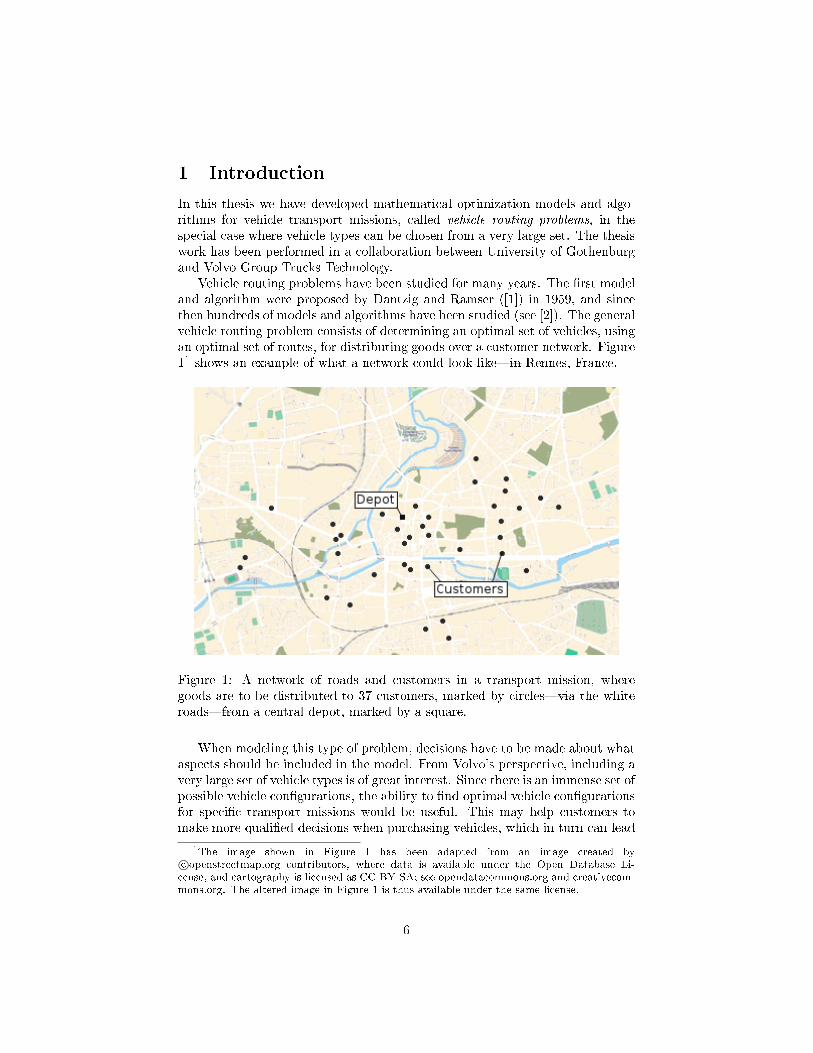
Vehicle routing problems have been studied for many years. The �rst modeland algorithm were proposed by Dantzig and Ramser ([1]) in 1959, and sincethen hundreds of models and algorithms have been studied (see [2]). The generalvehicle routing problem consists of determining an optimal set of vehicles, usingan optimal set of routes, for distributing goods over a customer network. Figure11 shows an example of what a network could look like�in Rennes, France.
Figure 1: A network of roads and customers in a transport mission, wheregoods are to be distributed to 37 customers, marked by circles�via the whiteroads�from a central depot, marked by a square.
When modeling this type of problem, decisions have to be made about whataspects should be included in the model. From Volvo's perspective, including avery large set of vehicle types is of great interest. Since there is an immense set ofpossible vehicle con�gurations, the ability to �nd optimal vehicle con�gurationsfor speci�c transport missions would be useful. This may help customers tomake more quali�ed decisions when purchasing vehicles, which in turn can lead
1The image shown in Figure 1 has been adapted from an image created byc©openstreetmap.org contributors, where data is available under the Open Database Li-cense, and cartography is licensed as CC BY-SA; see opendatacommons.org and creativecom-mons.org. The altered image in Figure 1 is thus available under the same license.
6

to more satis�ed customers. This type of optimization tool can also help Volvoto better understand their customers' needs, which may then in�uence strategicvehicle development decisions and make Volvo even more competitive on thetough global vehicle market.
Research on vehicle routing problems has been successful, and has proved tobe relevant in industrial applications. There is a growing industry of software fortransportation planning based on methods developed by the scienti�c commu-nity for vehicle routing problems, and increasingly complex models and largersized problems are solved ([3]). In this thesis, the focus is on �nding modelsand algorithms appropriate for vehicle routing problems with a very large set ofvehicle types. We have taken as a starting point so called heterogeneous vehiclerouting problems, hVRP, in which it is assumed that more than one vehicle typeis available. In previous hVRP models, to the best of our knowledge only a fewvehicle types have been included. We have adapted these models and algorithmsto accomodate a much larger set of vehicle types, here denoted many-hVRP. Inaddition, some new models and algorithms are proposed. Load dependent costs,which are not included in the standard hVRP, have also been implemented toillustrate how the solution framework developed can be expanded to includemore aspects of real transportation problems.
To solve the many-hVRP, exact algorithms and heuristics based on columngeneration, dynamic programming and Benders' decomposition will be used.These three mathematical optimization techniques are presented in Section 2.A literature review of modeling and solution approaches for relevant vehiclerouting problems is found in Section 3, problem formulations for many-hVRPare presented in Section 4 together with the implemented algorithms, after whichtests and results are presented in Section 5. Finally, a discussion of the resultsand some suggestions for further research are presented in Section 6.
7

2 Mathematical optimization techniques applica-
ble to vehicle routing problems
In optimization, problems are classi�ed into di�erent types that share certaincharacteristics and that can be solved using similar algorithms. Problems thatcan be stated as to
minimizex
c>x, (1a)
subject to Dx = d, (1b)
x ≥ 0n, (1c)
for c, x ∈ Rn, d ∈ Rm and D ∈ Rm×n�see Appendix A for an explanationof the notation is used in this thesis�are called linear optimization problemsor linear programs2. A vector x ∈ Rn that satis�es the constraints (1b)�(1c)is called a feasible solution. The aim is thus to minimize the linear objectivefunction c>x over the set of feasible solutions. The problem is said to be feasibleif there exists at least one feasible solution. The matrix D is called the constraintmatrix.
If the variables in the model (1) are required to be integer or binary, i.e. ifx ∈ Zn or x ∈ {0, 1}n, then we have an integer optimization problem/integerprogram [4].
Vehicle routing problems are often formulated as integer programs; see for-mulations (12) and (15) in Section 3.1.1. Integer programs can be computation-ally very hard to solve�much harder than linear programs. We present threealgorithms that can be used to solve integer programs, all of which have beenapplied to the many-hVRP in this thesis, as reported in Section 4. Columngeneration, which is presented in Section 2.1, is a method that solves linearprograms, and which is not guaranteed to �nd an optimal solution to an integerprogram unless it is combined with, for instance, a branch-and-bound algo-rithm. Column generation has previously and with great success been appliedto vehicle routing problems ([5]). In Section 2.2 dynamic programming is pre-sented, which is a technique that is especially suited to solve the subproblemsthat occur in column generation for vehicle routing problems. Benders' decom-position algorithm, which can solve integer programs to optimality, is presentedin Section 2.3. To the best of our knowledge, Benders' decomposition has notpreviously been applied to the hVRP; it has, however, been applied to otherrelated problems, such as the simultaneous aircraft routing and crew schedulingproblem ([6]) and network optimization problems (see [7]).
2.1 Column generation
The following outline of column generation is based on [8] and [9, Chapter 3.3],in addition to the textbook [4]. A more detailed account is found in Appendix
2The problem (1) can be formulated in di�erent ways. For instance, the constraints (1c)can be excluded since they can be incorporated into the constraints (1b), and the equality in(1b) can be replaced by two inequalities.
8
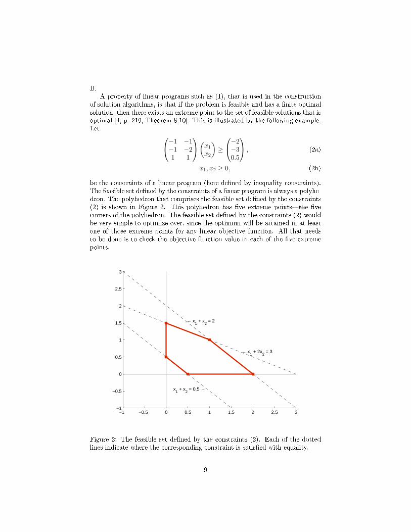
B.A property of linear programs such as (1), that is used in the construction
of solution algorithms, is that if the problem is feasible and has a �nite optimalsolution, then there exists an extreme point to the set of feasible solutions that isoptimal [4, p. 219, Theorem 8.10]. This is illustrated by the following example.Let −1 −1
−1 −21 1
(x1
x2
)≥
−2−30.5
, (2a)
x1, x2 ≥ 0, (2b)
be the constraints of a linear program (here de�ned by inequality constraints).The feasible set de�ned by the constraints of a linear program is always a polyhe-dron. The polyhedron that comprises the feasible set de�ned by the constraints(2) is shown in Figure 2. This polyhedron has �ve extreme points�the �vecorners of the polyhedron. The feasible set de�ned by the constraints (2) wouldbe very simple to optimize over, since the optimum will be attained in at leastone of those extreme points for any linear objective function. All that needsto be done is to check the objective function value in each of the �ve extremepoints.
−1 −0.5 0 0.5 1 1.5 2 2.5 3−1
−0.5
0
0.5
1
1.5
2
2.5
3
x1 + x
2 = 0.5 →
← x1 + x
2 = 2
← x1 + 2x
2 = 3
Figure 2: The feasible set de�ned by the constraints (2). Each of the dottedlines indicate where the corresponding constraint is satis�ed with equality.
9

For bigger linear programs, however, the feasible set can have a huge numberof extreme points. One solution technique that is used to solve such problems, iscalled the simplex method. To use the simplex method, the linear program mustbe expressed on the form (1), where n ≥ m. The idea is to start in one extremepoint and in each step of the algorithm go to the neighbouring extreme pointthat is most promising with respect to the change of the objective function value.Determining the most promising extreme point can be done without having toexplicitly enumerate all of the extreme points, by utilizing the so called reducedcosts3, denoted ci, i = 1, . . . , n. While standing at one extreme point, thereduced cost ci measure how much the value of the objective function changesif the value of the variable xi is increased by one�for variables xi that hasthe value zero4�while moving in the direction of one particular neighbouringextreme point. If mini∈{1,...,n} ci ≥ 0, then the current extreme point is anoptimal solution.
If the constraint matrix D in problem (1) has many columns, thousands orperhaps even millions, by using column generation it is possible to solve theproblem to optimality while only considering a small subset of the columns. LetI ⊂ {1, . . . , n} be such that |I| ≥ m represent a subset of the columns in theproblem (1). The constraint matrix restricted to the columns in I is denotedDI := (di)i∈I , where di, i = 1, . . . , n denote the columns of D. De�ninganalogously, cI := (ci)i∈I and xI := (xi)i∈I , we have the following model,having much fewer columns/variables than the model (1):
minxI
c>I xI , (3a)
s.t. DIxI = d, (3b)
xI ≥ 0|I|. (3c)
The model (3) is called the restricted master problem, in contrast to the com-plete problem (1) which is called the master problem. Here, the number ofcolumns/variables can be much smaller than in the master problem, i.e., |I| � n.The restricted master problem is feasible if the original problem (1) is feasibleand rank(DI) = m.
The column generation algorithm iteratively solves the restricted masterproblem, and uses information about its optimal solution to extend the set I,after which the restricted master problem is solved again. This is repeateduntil the optimal solution to the restricted master problem is veri�ed to beoptimal also in the master problem. The column generation subproblem uses thereduced costs to extend I and verify optimality, similarly to the simplex method,as described above. Given an optimal extreme point to the restricted masterproblem, using the corresponding optimal solution π∗ to its linear programming
3The reduced costs are de�ned in Appendix B.1.4For a linear program on the form (1) with n ≥ m, it holds that every extreme point
corresponds to at most m non-zero variable values xi, i = 1, . . . , n.
10

dual5, which is given by
maxπ
d>π,
s.t. D>I π ≤ cI ,
where π ∈ Rm, the reduced costs of the master problem variables xi, i =1, . . . , n, are given by
ci := ci − d>i π∗, i = 1, . . . , n.
Since the reduced costs measure how much the objective function value decreasesif the corresponding variable is increased by one, by adding a variable i ∈{1, . . . , n} \ I with strictly negative reduced cost ci to the restricted masterproblem (3), the optimal solution to (3) would be improved (unless the currentoptimal extreme point is degenerate, in which case it may not be possible totake a non-zero step in the direction de�ned by the new variable). Thus, todetermine which column to add to the restricted master problem, the problem,
c∗ := mini∈{1,...,n}
{ci} = mini∈{1,...,n}
{ci − d>i π
∗} , (4)
called the subproblem is solved, and the set I is extended by adding an indexi ∈ argmini∈{1,...,n} {ci}. If all the reduced costs are non-negative, i.e., if c∗ ≥ 0,then the current solution to the restricted master problem is also optimal in thecomplete master problem. This holds even if not all columns di, i = 1, . . . , n,have been generated, i.e., even if I 6= {1, . . . , n}. This means that the linearprogram can be solved while only generating a fraction of all its columns.
For integer programs, it is possible to apply column generation by relaxingthe integrality requirement. Solving the relaxed problem using column genera-tion not only gives a lower bound on the optimal value of the original integerprogram, but can also give a feasible (but not necessarily optimal) solution tothe integer program. The latter is achieved by, as a last step, solving the in-teger program using only the columns generated during the column generationprocess�this restricted master problem with integer requirements on the vari-ables can be much easier to solve than the original integer program if the number|I| of columns is large. See Appendix B.2 for details.
For problems that can be formulated as a set partitioning problem withbinary variables, column generation has been shown to be a good solutionstrategy�for vehicle routing and crew pairing assignment problems, among oth-ers. It is often implemented in combination with a branch-and-bound algorithm,called branch-and-price, in which an optimal integer solution is found using thelower bounds from column generation in each node ([5]). The most successfulexact algorithms for vehicle routing problems are based on branch-and-pricewith additional cut generation, so called branch-and-cut-and-price (see [10]).
5The dual of a linear program is the Lagrangian dual problem of the linear program (calledthe primal), see the textbook [4], and many useful relationships between the primal problemand the dual problem exists.
11

In this master thesis branch-and-price has not been implemented, but the col-umn generation algorithm can be improved by adding such a branch-and-boundframework.
2.2 Dynamic programming for shortest path problems with
resource constraints
The column generation subproblem (4) for vehicle routing problems are ele-mentary shortest path problems with resource constraints (denoted ESPPRC in[11]). These problems are NP-hard in the strong sense ([11, 12]), which makesit important to �nd e�cient solution strategies. Dynamic programming is themost commonly used method for solving subproblems when column generationis used in connection with vehicle routing problems ([12, p. 155]), although dueto the complexity of the problem often only a relaxed non-elementary shortestpath problem with resource constraints (denoted SPPRC in [11]) is solved, inwhich case it has a pseudo-polynomial complexity ([13]).
In the following subsections the dynamic programming algorithm for ESP-PRC is presented, along with some methods that can be implemented to makethe solution process more e�cient. Some of these methods for improving thealgorithm have been tested in this project (as detailed in Section 4.1.1) whileother methods are left as suggestions for further research (see Section 6.1).
2.2.1 A dynamic programming algorithm for ESPPRC
The following presentation is based on [11, 13].A general shortest path problem with resource constraints is de�ned on a
network of nodes N := {1, . . . , N}, arcs A ⊆ N × N , and a set of resources{1, . . . , R}. A path is a sequence of nodes, denoted Pi0iH := (i0, . . . , iH), whereih ∈ N , h = 0, . . . ,H, and (ih−1, ih) ∈ A, h = 1, . . . ,H. For i ∈ N , the notation(i) will be used to denote a single-node path. The set VPi0iH
:= {i0, . . . , iH} iscalled the set of visited nodes. A path Pi0iH can be extended by adding a nodeiH+1 ∈ N . The extended path is denoted (Pi0iH , iH+1). A similar notation isused for two paths that are concatenated.
Each path Pi0iH has an associated cost, denoted CPi0iH. The resource con-
sumption vector(T 1ih, . . . , TRih
)Pi0iH
∈ RR, for a given path Pi0iH at node ih,
represents the amount of each resource r ∈ {1, . . . , R} that has been consumedat node ih. The individual elements of the resource consumption vectors asso-ciated with path Pi0iH , are written as T rih(Pi0iH ), h = 1, . . . ,H, r = 1, . . . , R.The resource consumption vector
(T 1i0, . . . , TRi0
)Pi0iH
is given for the inital node
i0. Resource functions fr : RR ×A 7→ R are given, so that for h ∈ {1, . . . ,H},r ∈ {1, . . . , R},
T rih(Pi0iH ) := fr(
(T 1ih−1
, . . . , TRih−1)Pi0iH
, (ih−1, ih)).
12

For each node i ∈ N , a set of feasible resource consumption vectors
Ti :={
(T 1i , . . . , T
Ri )∣∣ T ri ∈ [ari , b
ri ], r ∈ {1, . . . , R}
},
is given. A path Pi0iH is said to be feasible with respect to the resource con-straints, or resource feasible, if for each node ih, h = 1, . . . ,H, it holds that(T 1ih, . . . , TRih
)Pi0iH
∈ Tih .The objective of the shortest path problem with resource constraints is to
minimize the cost CPst, over the set Pst of paths from node s ∈ N to node
t ∈ N , that are resource feasible.Dynamic programming is based either on the Ford-Bellman algorithm, or on
Djikstra's algorithm, depending on how paths are extended (see e.g. [13]). For ageneral shortest path problem with resource constraints, dynamic programmingcan work as follows ([11, 13]):
Paths starting at node s and ending in node i 6= t are maintained in a familyof non-processed paths, denoted PNPP, which at the beginning of the algorithmcontains only the single-node path (s). A path Psi ∈ PNPP is processed byextending it to all nodes j ∈ {j ∈ N , such that (Psi, j) is resource feasible.Each resulting path that does not end in node t is added to PNPP, while pathsending in t are added to a set of processed paths, denoted PPP. After path Psihas been processed, it is added to PPP. Extending paths in this way ensuresthat all paths, in PNPP as well as in PPP, are resource feasible.
From here on, Ui0iH , Qi0iH and Q∗i0iH are de�ned analogously to Pi0iH . LetEPsi
:= {(Psi, Ujt) | (Psi, Ujt) is resource feasible}, so that EPsiis the set of all
feasible extensions of the path Psi, ending in node t. For the paths Qsi and Q∗si,
both ending at the node i 6= t, Q∗si is said to be dominated by Qsi if
minPst∈EQsi
CPst≤ minPst∈EQ∗
si
CPst.
This means that no path in EQ∗sican have a lower cost than the best extension
(Qsi, Ujt) of Qsi. A path in PNPP ∪ PPP that is dominated by another path inthe same set can be removed.
When the set of non-processed paths PNPP is empty, an optimal path froms to t is found among the paths in PPP.
A simple example of a shortest path problem with resource constraints isshown in Figure 3. It contains �ve nodes and one resource. In the context ofvehicle routing problems, this resource may correspond to the available time fortraveling to the nodes of the network. Next to each arc (i, j), the arc cost cijand the resource consumption tij along that arc are shown in red. The resourceconsumption vectors are given by (T 1
1 )(1) := 0,(T 1j
)(P1i,j)
:=(T 1i
)P1i
+ tij ,
i, j ∈ {2, . . . , 5}, (i, j) ∈ A. The set of feasible resource consumption vectorsare de�ned by [a1
i , b1i ] := [0, 20], i = 1, . . . , 5. The costs are given by C(1) := 0,
C(P1i,j) := CP1i+ cij , i, j ∈ {2, . . . , 5}, (i, j) ∈ A.
13

The cheapest path from node 1 to node 5, disregarding resource consump-tion, is (1, 2, 3, 5), with the associated cost C(1,2,3,5) = 0.43. However, the path(1, 2, 3, 5) is not resource feasible, since
(T 1
5
)(1,2,3,5)
= 22 > 20. The cheapest
(shortest) path from node 1 to node 5, that is also resource feasible, is (1, 3, 5),with the cost C(1,3,5) = 0.88. For this example, dynamic programming is notvery useful since the optimal path can be found easily by inspection. For morecomplicated networks, the e�ciency of the dynamic programming algorithm de-pends strongly on the ability to �identify and discard paths which are not useful�[11, p. 46]. In the extreme case where no paths can be discarded (i.e. removeddue to domination), then dynamic programming is simply an enumeration offeasible paths, which is not a very e�cient algorithm.
1
2
3
4
5
(1.5,9)
(0.55,4)
(−1.4,6)
(1.8,3)
(0.33,7)
(0.24,3)
Figure 3: A network consisting of �ve nodes and six arcs, with one resource T 1.Each arc (i, j) has an associacted consumption tij of resource T 1, and a costcij , shown next to the arcs as (tij , cij). The resource T 1 is accumulated alongeach path, and the resource constraints state that T 1
i ∈ [0, 20], i ∈ {1, ..., 5}.
For an ESPPRC, paths must be elementary, meaning that no node i ∈N may be visited more than once. For (non-elementary) SPPRC with non-decreasing resource functions and with cost given by C(s) := c0, C(Psi,j) :=CPsi
+ cij , i, j ∈ N , (i, j) ∈ A, for paths Qsi and Q∗si which end in the samenode i, if the inequality6(
T 1i , . . . , T
Ri
)Qsi≤(T 1i , . . . , T
Ri
)Q∗si
holds, then Q∗si is dominated by Qsi and can be discarded. For ESPPRC withnon-decreasing resource fucntions, the set of visited nodes VQsi of Qsi must alsobe a subset of the visited nodes VQ∗si
of Q∗si, for Q∗si to be dominated by Qsi
(see [11, p. 50]). This is formalized in Claim 1, the proof of which is essentiallythe same proof as that of [13, Claim 1]. Claim 1 is the basis for the criteria for
6The notation`T 1
i , . . . , TRi
´Qsi
≤`T 1
i , . . . , TRi
´Q∗si
means T ri (Qsi) ≤ T r
i (Q∗si), ∀r ∈
{1, . . . , R}.
14

dominating paths in the dynamic programming algorithm used in this masterthesis. The speci�c details of this implementation are given in Section 4.1.1.
Claim 1. For an elementary shortest path problem with resource constraints,starting in node s ∈ N and ending in node t ∈ N , assume that the resourceconsumption is given by
T rj ((Psi, j)) := max{ari , T
ri (Psi) + hrij
},
where hrij ≥ 0, i, j ∈ N , (i, j) ∈ A, r ∈ {1, . . . , R}, and that the cost is given by
C(Psi,j) := CPsi+ cij , i, j ∈ N , (i, j) ∈ A
where C(s) := c0. For two elementary and resource feasible paths Qsi and Q∗si
ending in node i 6= t, Q∗si is dominated by Qsi if the relations(T 1i , . . . , T
Ri
)Qsi≤(T 1i , . . . , T
Ri
)Q∗si
,
CQsi ≤ CQ∗si,
andVQsi
⊆ VQ∗si
hold.
Proof. Since i 6= t, it holds that VQ∗si( N . If
(T 1j , . . . , T
Rj
)(Q∗si,j)
/∈ Tj for all j ∈N \VQ∗si
, then Q∗si can not be extended further. Otherwise, pick any j ∈ N \VQ∗si
for which(T 1j , . . . , T
Rj
)(Q∗si,j)
∈ Tj . The inclusion VQsi ⊆ VQ∗siimplies that the
extension (Qsi, j) is an elementary path. It holds that(T 1j , . . . , T
Rj
)(Qsi,j)
∈ Tj ,since for r ∈ {1, . . . , R},
T rj ((Qsi, j)) := max{ari , T
ri (Qsi) + hrij
}≤ max
{ari , T
ri (Q∗si) + hrij
}= T rj ((Q∗si, j)) ≤ bri .
It also holds that
C(Qsi,j) = CQsi + cij ≤ CQ∗si+ cij = C(Q∗si,j)
.
Hence, both (Qsi, j) and (Q∗si, j) are resource feasible elementary paths, and therelations (
T 1i , . . . , T
Ri
)(Qsi,j)
≤(T 1i , . . . , T
Ri
)(Q∗si,j)
,
C(Qsi,j) ≤ C(Q∗si,j),
andV(Qsi,j) ⊆ V(Q∗si,j)
hold. By induction with respect to extension of paths, any feasible extension(Q∗si, U
∗ij) of Q∗si also provides a feasible extension (Qsi, U∗ij) of Qsi, for which
C(Qsi,U∗ij)≤ C(Q∗si,U
∗ij). This shows that Q∗si is dominated by Qsi.
15
It is clear that the dominance rule of SPPRC is more e�cient than thatof ESPPRC, since more paths can be dominated if the restriction on visitednodes is left out. To increase the number of paths that can be eliminated forESPPRC�if it is possible to determine nodes that are unreachable from a givenpath using time-windows, for instance�unreachable nodes can be added to theset of visited nodes, which makes the dominance rule in Claim 1 a bit moree�cient ([11, pp. 50�51]).
2.2.2 Simplifying the problem
Relaxing the ESPPRC to the SPPRC by allowing paths containing cycles, i.e.,non-elementary paths, will result in problems having a larger state space butalso more e�cient dominance rules. When column generation is used as part ofthe solution procedure for vehicle routing problems, by using branch-and-pricefor instance, the lower bounds of the original problem provided by column gen-eration are weaker when the ESPPRC subproblems are relaxed to the SPPRC.This may be compensated by the reduction of the complexity of the subproblem,which can be great. A compromise between SPPRC and ESPPRC that is oftenimplemented for vehicle routing problems is to allow non-elementary paths, butforbid cycles of length two. This only duplicates the number of labels comparedto SPPRC and is quite easy to implement.
A compromise between the ESPPRC and the SPPRC has been proposed, inwhich, after solving the SPPRC, a restriction is imposed on the nodes that arevisited more than once. This new problem is solved, and analogous restrictionsare added to every node that is visited several times in the new solution. Thisprocedure is repeated until an elementary path is returned. In the worst casescenario, restrictions have to be added to all nodes.
Yet another way to simplify the ESPPRC is to use a so-called state-spacerelaxation. Instead of keeping track of the visited nodes, the number of visitednodes are used in the dominance criterion. This is di�erent relaxation of theESPPRC, and also in this case an elimination of cycles of length two can beimplemented (see [14, pp. 417�418] and [12, pp. 160�161,165]).
2.2.3 Heuristic methods for the ESPPRC
A heuristic for improving the speed of column generation, when using dynamicprogramming to solve the ESPPRC subproblems, can be implemented in severalways.
The dynamic programming algorithm can be terminated before an optimalpath has been veri�ed, and return a path with a negative reduced cost whichis not necessarily optimal. Since adding any path with a negative reduced costmay improve the solution in the next iteration of the column generation, it isonly necessary to solve the ESPPRC subproblem to optimality when trying toprove that the current solution to the restricted master problem is optimal in thecomplete problem. This does not need to be done at all when using a heuristiccolumn generation procedure.
16

Another heuristic approach is to temporarily relax the requirement thatpaths be elementary, and allow non-elementary paths in the beginning of thedynamic programming process. When paths get longer than a certain thresholdvalue, the elementarity requirement is added in the hope that an elementarypath with negative reduced cost is returned. If no such paths are found, theprocess is restarted and the elementarity requirement is added earlier than be-fore. This is repeated until an elementary path with negative reduced cost isfound (see [11, pp. 58�59]).
Betinelli et al. ([15]) take a di�erent approach, solving the ESPPRC columngeneration subproblems in three steps. The �rst step is a simple heuristic. Inthe second step, the domination requirement (see Claim 1) that the inclusionVQsi ⊆ VQ∗si
holds is relaxed, and replaced by another requirement. This resultsin a problem that is easier to solve but in which a path that is optimal inthe original, non-relaxed, problem may be dominated by a non-optimal path.Hence, optimality in the original problem, is not guaranteed in the solutionto the relaxed problem. In a �nal step, the relaxed criterion VQsi
⊆ VQ∗siis
reinstated, and the column generation subproblems are solved to optimality.
2.3 Benders' decomposition
To handle the large set of vehicle types inmany-hVRP, decomposing the problemin several levels can be a good idea. Using Benders' decomposition, problemscan be decomposed in such a way that in each iteration one set of variables�which we call complicating variables�are �xed, and the problem with respectto the remaining variables is solved to optimality. This procedure is iterated,so that information about solutions from previous iterations is used to �x thecomplicating variables in each iteration, until the optimal solution to the re-stricted problem (with �xed variables) is veri�ed to be an optimal solution tothe original problem.
In the context of many-hVRP, the complicating variables can be chosen tobe the vehicle types, so that in each iteration a subset of the vehicle types�ofa size that can be e�ciently handled�is chosen among the whole set of vehicletypes. The details of our implementation of Benders' algorithm for many-hVRPis presented in Section 4.2.
For routing and scheduling problems arising in areas such as airline planning,Benders' decomposition together with column generation has successfully beenapplied by Cordeau et al. in [6] to simultaneously consider both the aircraftrouting problem and the crew pairing problem�something that traditionallyhave been done sequentially due to the large complexity of the problem. Theirimplementation �rst uses a linear programming (LP) relaxation of both Bendersmaster problem and Benders subproblem, and later reintroduces the integer re-quirements and performs a heuristic branching on the integer variables. Branch-ing on variables has not been performed in this thesis, however it would be aninteresting extention of the implemented algorithm. The review [16] of airlinescheduling planning, by Dunbar et al., describes how the method by Cordeau etal. ([6]) has been expanded and improved by several authors. The expansions
17

include time windows, reversing the order of Benders master- and subproblemswhich improved the convergence rate, and applying a heuristic algorithm toparts of the problem to avoid the tailing o�-e�ect of column generation.
Here, a version of Benders' decomposition that in this thesis is used onmany-hVRP is presented. The theory is based on [9, Chapter 7.3]. The goal isto solve an optimization problem of the form
minx,y
c>x, (5a)
s.t. Dx + Fy = b, (5b)
x ≥ 0n1 , (5c)
y ∈ {0, 1}n2 , (5d)
for c, x ∈ Rn1 , y ∈ Rn2 , b ∈ Rm and D ∈ Rm×n1 , F ∈ Rm×n2 . The set offeasible solutions to (5) is assumed to be non-empty and bounded. Here, thecomplicating variables are the binary variables y. If variables y are �xed, theremaining problem is a linear program, which is assumed to be much easier tosolve than the integer program (5). De�ning the set R := {y ∈ {0, 1}n2 | ∃x ≥0n1 ,Dx = b − Fy}, a formulation that is equivalent to the model (5) is givenby
miny∈R
{minx
c>x∣∣∣ Dx = b− Fy,x ≥ 0n1
}. (6)
The inner problem, given by
minx
c>x, (7a)
s.t. Dx = b− Fy, (7b)
x ≥ 0n1 , (7c)
is called Benders subproblem. The feasible set of (7) is non-empty and boundedfor y ∈ R. Due to strong duality for linear programs, which says that theoptimal objective value of (7) for �xed y ∈ R is equal to the optimal objectivevalue of its dual [4, p. 248], (7) can be replaced by its dual
maxu
(b− Fy)>u, (8a)
s.t. D>u ≤ c, (8b)
u ∈ Rm. (8c)
This problem is also feasible and bounded for y ∈ R, so there exists an optimalsolution in at least one of the extreme points of its feasible set. It can thus bereformulated as
maxi∈P
{(b− Fy)> ui
}, (9)
18

where the set {ui, i ∈ P} denotes the extreme points of the set {u | D>u ≤ c}.The model (6) can now be written as
miny∈R
{maxi∈P
{(b− Fy)> ui
}},
which in turn can be reformulated as
v∗BMP := miny,v
v, (10a)
s.t. v ≥ (b− Fy)> ui, i ∈ P, (10b)
y ∈ R. (10c)
The problem (10) is called Benders master problem. As with column genera-tion7, a restricted version of this problem is introduced where in this case onlya subset of the constraints are included, resulting in Benders restricted masterproblem
v∗BRMP := miny,v
v, (11a)
s.t. v ≥ (b− Fy)> ui, i ∈ P, (11b)
y ∈ R, (11c)
where P ⊆ P. For (v∗BMP,y∗) optimal in Benders master problem it holds that
v∗BMP equals the optimal objective value of the original problem (5), and solvingBenders subproblem (7) with y := y∗ will yield x∗, for which (y∗,x∗) is optimalin the original problem.
Since not all constraints are included in Benders master problem, the in-equality v∗BRMP ≤ v∗BMP holds if (v∗BRMP, y
∗) is optimal in (11). Such an optimal
solution (v∗BRMP, y∗) exists and is bounded if P 6= ∅, since R is closed, bounded,
and non-empty. Solving Benders subproblem (7) with y := y∗ provides a feasi-ble solution (y∗, x∗) to the original problem, and c>x∗ is consequently an upperbound on its optimal value v∗BMP. Solving the dual (9) of Benders subproblem,again with y := y∗, provides an extreme point ui∗ , i∗ ∈ P, for which the equiv-alence (b− Fy∗)> ui∗ = c>x∗ holds. This is an upper bound on the optimalvalue v∗BMP, and for which v∗BRMP is a lower bound. Thus, if it holds that
(b− Fy∗)> ui∗ = v∗BRMP,
then (y∗, x∗) is an optimal solution to the original problem (5). Otherwise, theinqualities
(b− Fy∗)> ui∗ ≥ v∗BMP ≥ v∗BRMP,
hold and i∗ is added to P de�ning a new constraint to Benders restricted masterproblem. Since ui∗ is optimal in (9), the new constraint is the constraint in Ben-ders master problem which is the most unsatis�ed by the solution (v∗BRMP, y
∗).7If the problem (5) were linear, i.e., if the constraint (5d) was replaced by y ≥ 0n2 , then
Benders' algorithm would be equivalent to applying Dantzig-Wolfe decomposition and columngeneration to the dual of (5). See [9, Chapter 7.3.2] for details.
19

Solving Benders restricted master problem with the updated set of constraintswill yield a solution that is di�erent from (v∗BRMP, y
∗), which is no longer feasi-ble, and the new optimal objective value of Benders restricted master problemwill be greater than or equal to v∗BRMP. Since the number of constraints inBenders master problem is �nite, Benders' algorithm is guaranteed to convergein a �nite number of iterations.
20
3 Vehicle routing problems
Vehicle routing problems are di�cult optimization problems, which have appli-cations in many �elds, including transportation, logistics, communication andmanufacturing, and they belong to the most studied combinatorial optimizationproblems. The classic problem called the capacitated vehicle routing problem,cVRP, consists of �nding a solution to a simpli�ed transport mission in whichcustomers are serviced by a set of indentical vehicles delivering goods from acentral depot, where the number of customers that each vehicle can service islimited by a vehicle capacity restriction. The cVRP is an extension of the trav-eling salesman problem, and is NP-hard in the strong sense (see e.g. [3, 17, 18]).
A wide range of extensions of the classic cVRP are available and severalthousands of articles have been dedicated to the subject. These extensions canbe classi�ed into the three main groups
1. Assignment of customers and routes to resources, including multiple de-pots, a heterogeneous �eet of vehicles, multiple periods, in which customersare serviced more than once, and split deliveries, in which customers canbe serviced by more than one vehicle.
2. Sequence choices, including backhauls and pickup-and-delivery where de-liveries are made to one set of customers and goods are picked up from a setof vendors/customers, and orders can be recieved dynamically, precedenceconstraints such that some customers should be serviced before others,and multiple trips, in which vehicles can depart from and return to thedepot more than once.
3. Evaluation of �xed sequences, including time windows where each cus-tomer needs to be serviced within a given time-frame, networks with time-dependent features such as time-dependent travel times or time-dependentservice costs, and 2D and 3D loading constraints. [3]
Many di�erent solution methods, both exact and heuristic, have been developedfor di�erent types of vehicle routing problems, and even though the methodsneed to be tailored to the speci�c problem, several methods can be applied todi�erent extensions of cVRP. Consistently, exact methods for vehicle routingproblems can only solve problems with up to 200 customers (see [3, 10, 18]).
Successful heuristic methods for vehicle routing problems almost always usea combination of di�erent classical heuristics. Recently, combinations of ex-act methods�based on mathematical programming techniques�and heuristicmethods, have been proposed. These are sometimes called matheuristics (see[10]). According to [10], p. 61 �an exact solution of real-world problems withmany additional side constraints will remain impossible in the short and mediumterm. However, close-to-optimal solutions of more and more complex and inte-grated problems, increasingly based on incomplete optimization approaches andmathematical-programming-based heuristics, are possible, and this is su�cientto provide useful decision support in practice�.
21

In this thesis we are interested in vehicle routing problems with a very largeset of vehicle types, which we call many-hVRP, in constrast to the standardvehicle routing problem with a heterogeneous �eet, hVRP, in which usually onlya few vehicle types are considered. The sets of vehicle types for many-hVRPcould be so large that it would not be practical to consider the whole set, makingthe algorithms that have previously been used for hVRP impractical. Parts ofthe models and algorithms for many-hVRP have been based on mathematicalprogramming algorithms developed for hVRP, which are presented in Section3.1. In Section 3.2 a model including load dependent costs which has beenincorporated into the many-hVRP model, is presented. Other extensions suchas time-windows can easily be implemented. Algorithms for many-hVRP arepresented in Section 4.
3.1 Heterogeneous vehicle routing problems
The vehicle routing problem with a set of non-identical vehicle types was �rstformulated by Golden et al. ([19]) in 1984. The problem is known as the het-erogeneous VRP, or the �eet size and mix VRP (see [17]).
When modeling real-life problems, there is often a trade-o� between the num-ber of practical considerations that can be included and the maximum problemsize that can be solved within a reasonable amount of time. A heterogenous�eet of vehicles is one such aspect of real-life problems that may be importantto consider. Ho� et al. state in [7, p. 2043] that �there is generally a strong de-pendency between �eet composition and routing aspects�, and decisions about�eet composition and routing need to be integrated. Given a transport mission,the optimal routing depends strongly on the characteristics of the available �eetof vehicles. Ho� et al. directs critisism against the operation research commu-nity, saying that it has been too focused on idealized models and that there hasnot been enough e�ort directed towards the �eet composition problem [7].
Nevertheless, there has been a number of contributions relating to hVRPfrom the operation research community. In the following sections standardmodels, solution methods and test instances for hVRP are presented.
3.1.1 Standard models
In hVRP a heterogeneous set of vehicles is considered, in constrast to cVRPwhere all vehicles are of the same type. Vehicle types di�er by their capacityand cost structure. A limited or unlimited number of vehicles of each type isavailable. One part of the cost of each route can be �xed (denoted �xed cost),and one part of the cost can depend the route length (denoted variable cost)�sometimes only a �xed cost or only a variable cost is used. Sometimes, thevariable cost does not depend on the vehicle type used for the route ([17]). Inthis thesis, no restriction has been put on the numbers of vehicles of each typethat are available, and a combination of �xed and variable costs is used�bothof which depend on vehicle type.
22

There exist three main types of mathematical models for vehicle routingproblems in general. In the �rst type, integer vehicle �ow variables are usedto model both the vehicle routes and the commodity �ow. In the second type,additional continuous variables are used to model the commodity �ow. The thirdtype of model uses a set-partitioning formulation. The �rst type of models hasmostly been used for basic versions of vehicle routing problems, and is accordingto Toth et al. [18], not suited for heterogeneous vehicle problems. Therefore,the second and third types of models of the hVRP is presented below. Theformulation using commodity �ow variables is from [7], and the set-partitioningformulation can be found in [20].
Both models are de�ned on a directed graph (N ,A), whereN :={0, 1, . . . , N}denotes the set of nodes representing the customers and the depot, and A de-notes the set of directed arcs between the nodes in N representing the network.The depot is denoted by 0, making N \ {0} =: N0 the set of nodes representingthe customers. Each customer i ∈ N0 has a demand di. There are K di�erentvehicle types, represented by the set K := {1, . . . ,K}. Each vehicle k has alimited capacity, denoted Dk. It is assumed that every customer may be servedby at least one vehicle type, i.e., the constraint maxk∈KDk ≥ maxi∈N di musthold.
Associated with each vehicle type k ∈ K are routing (or variable) costs ckij ,(i, j) ∈ A, and a �xed cost fk. In the model (12) feasible routes are de�nedby the constraints in the model, while in the model (15) feasible routes areimplicitly de�ned by the sets Rk, k ∈ K, containing all feasible routes r withrespect to vehicle type k. A route is a sequence of nodes (i0, i1, . . . , iH−1, iH),where ih ∈ N , h = 0, . . . ,H, and (ih−1, ih) ∈ A, h = 1, . . . ,H. A router := (i0, i1, . . . , iH−1, iH) is feasible if it starts and ends at the depot, i.e. ifi0 = iH = 0. A route-vehicle pair (r, k), such that r := (i0, i1, . . . , iH−1, iH),and k ∈ K, is feasible if the route is feasible and if the capacity constraintsof the vehicle type are satis�ed by the route, i.e., if the total demand�givenby∑H−1
1 dh�of the customers along the route is less than or equal to thevehicle's capacity Dk. The cost for a feasible route-vehicle pair (r, k) equals
ckr := fk +∑Hh=1 c
kih−1ih
.
Formulation using commodity �ow variables:
De�ne the variables
xkij :=
{1, if arc (i, j) is used by a vehicle of type k,
0, otherwise,(i, j) ∈ A, k ∈ K,
and eij := �ow of goods from node i to j, (i, j) ∈ A. The commodity �owformulation is given by:
23

minx,e
∑k∈K
∑j∈N :(0,j)∈A
fkxk0j +
∑k∈K
∑(i,j)∈A
ckijxkij
, (12a)
s.t.∑k∈K
∑i∈N :(i,j)∈A
xkij = 1, j ∈ N0, (12b)
∑i∈N :(i,j)∈A
xkij −∑
i∈N :(j,i)∈A
xkji = 0, j ∈ N0, k ∈ K, (12c)
∑i∈N :(i,j)∈A
eij −∑
i∈N :(j,i)∈A
eji = dj , j ∈ N0, (12d)
e0j ≤∑k∈K
Dkxk0j , (0, j) ∈ A, (12e)
eij ≤∑k∈K
Mijkxkij , (i, j) ∈ A, (12f)
eij ≥ 0, (i, j) ∈ A, (12g)
xkij ∈ {0, 1}, (i, j) ∈ A, k ∈ K. (12h)
The objective (12a) is to minimize the sum of the �xed costs and the routecosts of each vehicle used. The constraints (12b) ensure that each customeris visited exactly once, and the constraints (12c) that any vehicle that visitsa customer departs from that customer. The constraints (12d) ensure that avehicle that visits a customer delivers exactly the amount of goods that thecustomer demands. The constraints (12e)�(12f) impose the vehicle capacityrestrictions, where the parameter Mijk is chosen to be su�ciently large.
A slightly di�erent formulation is found in [17], in which constraints limitthe number of vehicles of each type, and the constraints (12e)�(12f) have beenreplaced by
djxkij ≤ eij ≤ (Dk − di)xkij , (i, j) ∈ A, k ∈ K. (13)
This formulation is not consistent, since xkij is always zero for some k ∈ K if|K| > 1. We suggest that the constraints (12e)�(12f) be replaced by
djxkij ≤ eij ≤ (Dk − di)xkij +Mijk(1− xkij), (i, j) ∈ A, k ∈ K. (14)
Set-partitioning formulation:
De�ne the parameters
δkir :=
{1, if route (r, k) visits customer i,
0, otherwise,i ∈ N0, r ∈ Rk, k ∈ K,
24

and the variables
xkr :=
{1, if route (r, k) is used,0, otherwise,
r ∈ Rk, k ∈ K.
The set-partitioning formulation is then given by:
minx
∑k∈K
∑r∈Rk
ckrxkr , (15a)
s.t.∑k∈K
∑r∈Rk
δkirxkr = 1, i ∈ N0, (15b)
xkr ∈ {0, 1}, r ∈ Rk, k ∈ K. (15c)
The objective (15a) is to minimize the sum of the costs over the routes thatare used. The constraints (15b) ensure that each customer is visited by exactlyone vehicle.
This type of set-partitioning formulation was originally proposed for the ve-hicle routing problem by Balinski and Quandt in 1964 ([21]). The model isgeneral, and has the advantage that many restrictions can easily be incorpo-rated, since the feasibility of routes is implicitly de�ned by the sets Rk, k ∈ K.The LP relaxation of this type of model for VRP is often very tight. Also, thenumber of feasible routes,
∑k∈K |Rk|, will for most problems be extremely big,
which makes column generation an appropriate solution method�for problemswith tens of customers, there may be billions of feasible routes ([18]). The set-partitioning formulation is then seen as a column generation master problem,where the column generation subproblems generate routes xkr to be added tothe the restricted master problem (in which not all routes in the sets Rk, k ∈ Kare included).
3.1.2 Previously developed solution strategies
Up until recently, no exact algorithm had been implemented for the hVRP �dueto the intrinsic di�culty of this family of routing problems� ([17, p. 13]). Exactsolution methods have now been developed based on branch-and-cut-and-priceby Pessoa et al. in 2007 ([22]) and on a set-partitioning formulation usingadditional constraints by Baldacci et al. in 2009 ([23]). The exact method in[23] can solve instances with up to 75 customers and some instances with 100customers; it works well for other types of vehicle routing problems as well ([3]).
Baldacci et al. review in [17] the many di�erent heuristic solution methodsthat have been applied to hVRP, as do Ho� et al. in [7]. Of the methodsreviewed, the set-partitioning based heuristic proposed by Taillard in [20] andthe column generation based heuristic of Choi and Tcha in [24] are of particularrelevance for this project; both methods are mentioned in both review articles[7, 17].
Taillard [20] implemented a set-partitioning based heuristic algorithm, thatsolves one homogeneous VRP (where only one vehicle type is allowed) for each
25

vehicle type using an adaptive memory procedure. From each homogeneousVRP a set of routes are stored. These routes are added as columns to a set-partitioning formulation of hVRP, but here each route r de�nes one column foreach vehicle type k for which r ∈ Rk�not just for the vehicle type(s) that theroute was associated with in the homogenous problem. Unfortunately, accordingto [20, p. 6], the method does not perform well on very small instances whenthe number of vehicles allowed of each vehicle type was restricted, in which case�there was a higher probability that a run would not produce a good or evenfeasible solution� compared to the larger instances.
Inspired by the approach in [20], in [24] Choi and Tcha presented a columngeneration based heuristic using the following set-partitioning formulation:
minx
∑k∈K
∑r∈Rk
ckrxkr , (16a)
s.t.∑k∈K
∑r∈Rk
δkirxkr ≥ 1, i ∈ N0, (16b)
∑r∈Rk
xkr = αk, r ∈ Rk, k ∈ K, (16c)
xkr ∈ {0, 1}, r ∈ Rk, k ∈ K, (16d)
αk ≥ 0, integer, r ∈ Rk, k ∈ K. (16e)
Compared to the formulation (15), the constraints (16c) and (16e) have beenadded to the set-partitioning problem, relating to the number αk of vehicles oftype k that is used. The new constraints do not impose any restriction on thenumber of vehicles that are allowed but are used to accelerate a branch-and-bound implementation. In addition, the problem is formulated as a set-coveringrather than a set-partitioning problem. Since arc costs correspond to Euclideandistances the two models are equivalent in the sense that the optimal solutionto (15) is optimal also in (16). The subproblems that generate new columns forthe restricted master problem corresponding to (16) are de�ned as
minr∈Rk,k∈K
(ckr −
∑i∈N0
π∗i δkir − π∗k
), (17)
where π∗i and π∗k are the optimal dual variable values corresponding to theconstraints (16b) and (16c), respectively. In [24] this subproblem is divided intoone subproblem for each vehicle type which are relaxed, both by a state-spacerelaxation and by relaxing the elementary constraint, while introducing a 2-cycle elimination procedure. The relaxed subproblems are solved using dynamicprogramming. It was found in [24] that only very small problem instances withup to 20 customers could be solved to optimality using this approach.
Therefore the column generation procedure is employed in a heuristic branch-and-bound algorithm. In a preprocessing step, some vehicle types are discardedby calculating a lower bound on the optimal value of (16) by requiring that atleast one vehicle of a particular type is used, taking only the �xed costs into
26

account. This lower bound is compared with an upper bound provided by aheuristic, enabling the rejection of the vehicle types for which the correspondinglower bound is higher than the upper bound of the original formulation (16) (see[24]).
This column generation algorithm by Choi and Tcha has been reported toprovide good results compared with other heuristic solution methods in the tworeview articles [17, 7]. In [7, p. 2048], it is stated that �results con�rm thedominance of this algorithm, both in terms of quality and computation time�.According to Pessoa et al. ([22]), who developed an exact branch-and-cut-and-price algorithm, the lower bounds computed by Choi and Tcha [24] were note�ective enough for an exact branching algorithm, but the columns generatedin the root node yielded a heuristic solution that outperformed other heuristicson several test instances.
The approach to solve hVRP heuristically implemented by Choi and Tchain [24] has been used as a starting point for the algorithms developed in thisthesis�both the splitting of the column generation subproblem into one problemper vehicle type and the solution of subproblems using dynamic programming�which will be explained in Section 4.1. The results obtained by the columngeneration algorithm implemented in this thesis are compared with the resultsin [24], and presented in Section 5.1.1.
3.1.3 Standard benchmarks
In 1984 Golden et al. ([19]) introduced test instances for the hVRP based oncustomer node data from instances found in [25, 26], which include twenty setsof test instances, twelve of which possessing Euclidean distances (denoted G12in [17]). The test instances in G12 are commonly used for hVRP with only�xed costs. Taillard ([20]), whose set-partitioning based heuristic is describedin Section 3.1.2, adapted eight of the twelve sets in G12 by de�ning variablecosts (denoted T8 in [17]). These are typically used as benchmarks to testalgorithm performance for hVRP with variable costs. None of the test instancesin G12 and T8 possesses a combination of �xed and variable costs of which bothdepend on the vehicle type ([17, 3]). Another set of test instances that should bementioned are those proposed by Li et al. in [27], containing 200�360 customerslocated on concentric circles around the depot, with four to six vehicle types ineach instance. These test instances are also frequently used as benchmarks forhVRP ([3]).
The algorithm presented in [24], also described in Section 3.1.2, was testedon extensions of the test instances T8 and G12. The eight instances that arecommon to the sets T8 and G12 were combined, so that both the �xed andvariable costs that depend on the vehicle type�from the respective sets T8 andG12�were applied simultaneously. The set T8 was also extended to include allof the instances in G12, by adding variable costs which depend on the vehicletypes to the four instances in G12 that were not included in T8. The four newinstances are the smallest in the set, with only 20 customers each (a reason whythey were not included in T8 may be that the algorithm implemented in [20]
27

did not perform well on small instances). The twelve new instances are heredenoted CT12. In [24], the algorithm was also tested on T8 and G12, to beable to compare with other published results. In [17], the best solution valuesobtained using di�erent heuristics are compared with the best known solutionsat the time (2008). The best known solutions was found by Choi and Tcha forall instances in T8 (see [17, Table 6]), and the average relative gap with respectto the best known solution values for instances in G12 was 0.004% (see [17,Table 4]). The best solutions known today (2014) for CT12 are presented inSection 5.1.1�better solutions than those obtained in [24] have only been foundfor two of the twelve instances in CT12.
The test instances CT12 have been used to test the performance of ouralgorithms, both in their original form and their extensions to include morevehicle types (presented below). Problem speci�cations for CT12 are listed inTable 18. The four test instances to which Choi and Tcha added vehicle speci�cvariable costs to are named Choi3�Choi6, and the instances from T8 are namedT13�T20, following the numbering of the original instances in [19]. The rangesof the capacities, the �xed costs, and the variable costs, for the vehicles in eachinstance are given in Table 1. For r ∈ Rk, k ∈ K, the cost ckr of the route-vehicle pair (r, k) is given by ckr := fk + vkαk, where fk denotes the �xed cost,vk denotes the variable cost, and αk denotes the length of the route r. A smallervehicle is always less expensive than a larger vehicle, i.e., for k1, k2 ∈ K, theinequality Dk1 < Dk2 implies the inequalities fk1 < fk2 and vk1 < vk2 . Foreach test instance in CT12, vehicles are denoted by letters, so that, e.g., the �vevehicles of test instance Choi3 are denoted A�E, where A (E) corresponds tothe vehicle with the smallest (largest) capacity.
Each of the twelve test instances in CT12 contains three to six di�erentvehicle types and 20�100 customers. The instances Choi3�Choi6 share customernodes N0 and customer demands. The di�erence between the instances Choi3�Choi4 and Choi5�Choi6 is that the depot has been moved. The instances T13�T14 also have the same node speci�cations, as do the instances T15�T16, T17�T18, and T19�T20, respectively.
To test the many-hVRP problem formulation, the instance set CT12 hasbeen extended to include vehicles with capacities in the ranges of the corre-sponding original instances Choi3�Choi6 and T13�T20. All integer values in thiscapacity interval have been included, since the demands of the customers are allinteger. The �xed and variable costs have been extended accordingly using thespline function in Matlab. The new set of test instances is denoted CT12EXT,and the individual test instances are denoted Choi3EXT�Choi6EXT, T13EXT�T20EXT. Consequently, the test instances in CT12EXT comprise 91�381 dif-ferent vehicle capacities. Accordingly, e.g., does Choi3EXT includes 101 vehicletypes with capacities ranging from 20 to 120, �xed cost ranging from 20 to 225,
8The instances CT12 can be constructed as follows; the instances in G12, are constructedusing the instances which were introduced by Christo�des et al. ([25])�these are downloadedfrom [28]. The networks of customer nodes of CT12 are constructed according to the instruc-tions given by Golden et al. [19] for G12, while the vehicle speci�cations for CT12 are setaccording to [24, Table 1] (which are also found in [23, Table 2]).
28
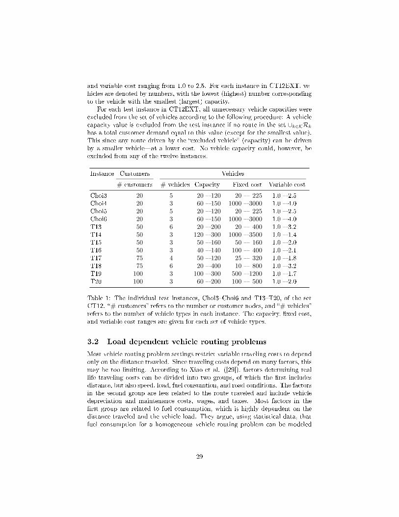
and variable cost ranging from 1.0 to 2.5. For each instance in CT12EXT, ve-hicles are denoted by numbers, with the lowest (highest) number correspondingto the vehicle with the smallest (largest) capacity.
For each test instance in CT12EXT, all unnecessary vehicle capacities wereexcluded from the set of vehicles according to the following procedure: A vehiclecapacity value is excluded from the test instance if no route in the set ∪k∈KRkhas a total customer demand equal to this value (except for the smallest value).This since any route driven by the �excluded vehicle� (capacity) can be drivenby a smaller vehicle�at a lower cost. No vehicle capacity could, however, beexcluded from any of the twelve instances.
Instance Customers Vehicles
# customers # vehicles Capacity Fixed cost Variable cost
Choi3 20 5 20 � 120 20 � 225 1.0 � 2.5Choi4 20 3 60 � 150 1000 � 3000 1.0 � 4.0Choi5 20 5 20 � 120 20 � 225 1.0 � 2.5Choi6 20 3 60 � 150 1000 � 3000 1.0 � 4.0T13 50 6 20 � 200 20 � 400 1.0 � 3.2T14 50 3 120 � 300 1000 � 3500 1.0 � 1.4T15 50 3 50 � 160 50 � 160 1.0 � 2.0T16 50 3 40 � 140 100 � 400 1.0 � 2.1T17 75 4 50 � 120 25 � 320 1.0 � 1.8T18 75 6 20 � 400 10 � 800 1.0 � 3.2T19 100 3 100 � 300 500 � 1200 1.0 � 1.7T20 100 3 60 � 200 100 � 500 1.0 � 2.0
Table 1: The individual test instances, Choi3�Choi6 and T13�T20, of the setCT12. �# customers� refers to the number or customer nodes, and �# vehicles�refers to the number of vehicle types in each instance. The capacity, �xed cost,and variable cost ranges are given for each set of vehicle types.
3.2 Load dependent vehicle routing problems
Most vehicle routing problem settings restrict variable traveling costs to dependonly on the distance traveled. Since traveling costs depend on many factors, thismay be too limiting. According to Xiao et al. ([29]), factors determining reallife traveling costs can be divided into two groups, of which the �rst includesdistance, but also speed, load, fuel consumtion, and road conditions. The factorsin the second group are less related to the route traveled and include vehicledepreciation and maintenance costs, wages, and taxes. Most factors in the�rst group are related to fuel consumption, which is highly dependent on thedistance traveled and the vehicle load. They argue, using statistical data, thatfuel consumption for a homogeneous vehicle routing problem can be modeled
29

by the following objective function
minx,e
∑j∈N
fx0j +∑
(i,j)∈A
(cijxij + bijeij)
(18)
and constraints corresponding to (12b)�(12h), but considering only one vehicletype. Analogously to the �ow formulation (12) for hVRP, the variables arede�ned as
xij :=
{1, if arc (i, j) is used0, otherwise
(i, j) ∈ A,
and eij := �ow of goods from node i to j, (i, j) ∈ A. Also, the parameters cij ,(i, j) ∈ A, are routing (variable) costs and the parameter f is a �xed cost. Inaddition, there are parameters bij , (i, j) ∈ A, which determines the contributionof the load across each arc to the total cost. Here cij and bij are parameters notonly depending on distance but also on fuel consumption rates and fuel prices,and the load variable eij is measured in weight units. The authors of [29] use asimulated annealing based heuristic algorithm to solve this homogeneous vehiclerouting problem.
The objective function (18) can easily be adjusted for the column generationsubproblems of hVRP or many-hVRP by letting f , cij , and bij depend on thevehicle type, since each vehicle type can be treated separately in the subprob-lems. This has been done in this thesis; see Section 4.3. It would be moredi�cult to use this type of load dependent cost function for a formulation suchas the �ow formulation (12) of hVRP. Making the parameters bij depend on thevehicle type would require the variables ekij , representing the load on the vehicleof type k on link (i, j), (i, j) ∈ A, k ∈ K.
30

4 Problem formulation and solution methods for
the many-hVRP
The many-hVRP problem, for which we wish to �nd a suitable model andsolution method, is the version of the standard hVRP where the number ofdi�erent vehicle types is very large. If some of the parameters that determinethe con�gurations of the vehicles can be chosen from a continuous interval, theremay even be an in�nite number of possible vehicle types.
The standard test instances for hVRP, some of which were presented inSection 3.1.3, contain relatively few vehicle types. To the best of our knowledge,hVRP with a very large set of vehicle types�here denoted many-hVRP�havenot been studied before. To e�ciently handle many-hVRP, solution techniquestailored for the large set of vehicles are necessary. Starting from the solutiontechnique for hVRP from [24], as presented in Section 3.1.2, a column generationalgorithm has been implemented for many-hVRP; it is presented in Section4.1. This implementation uses a straightforward adaptation of the hVRP model(15), and is therefore denoted the straightforward model. A slightly di�erentmodel, in which the number of vehicle types that can be used in a feasiblesolution is restricted, is presented in Section 4.2. There are two main reasonsfor formulating many-hVRP using this model, denoted the restricted model.The �rst reason is simply that a restriction on the number of vehicle types in asolution may be a desirable feature in a solution, when the set of vehicle typesis very large. A �eet with fewer vehicle types may for instance be more �exible.The second reason is due to algorithmic considerations. The restriction of thenumber of vehicle types used in a solution enables a Benders' decompositionof an LP relaxation of the model, which then results in a subproblem havingthe same form as the master problem in a column generation approach to thestraightforwad model. Benders subproblem can thus be solved using the columngeneration algorithm presented in Section 4.1 for the straightforward model,but with a smaller set of vehicle types. The number of vehicle types allowedin a feasible solution to the restricted model determines the size of the set ofvehicle types considered in Benders subproblem, in�uencing its computationalcomplexity.
To illustrate how these models adapt to more complex problem settings, thestraightforward and the restricted model, as well as the corresponding solutionalgorithms have been adapted to consider load dependent costs, following themodel presented in Section 3.2. The details are presented in Section 4.3.
To the best of our knowledge, the restriction on the number of vehicle typesused in a solution to the restricted model has not been used in previous modelsfor hVRP, probably because the number of vehicle types considered is usuallysmall. Neither have we encountered the application of Benders' algorithm tohVRP in the literature. We envision that the algorithms developed in thisthesis�with some modi�cations of the implementation of the sets of vehicletypes which showed to �t well within our current solution framework; see Sec-tion 6�can be successfully applied to real life instances of larger size than the
31
benchmarks CT12 and CT12EXT here used to test the algorithms.
4.1 The straightforward model with column generation
The heterogeneous vehicle routing problem can, as shown in Section 3.1.1, beformulated as the set-partitioning model (15). Hence, it can also be used tomodel the many-hVRP. Using the model (15) has the advantage that standardsolution methods that have been proven successful for hVRP can be appliedalso to many-hVRP. We denote the model (15), when used for many-hVRP,as the straightforward model. A version of the column generation approachimplemented in [24]�which has proved successful for hVRP; see Sections 3.1.2and 3.1.3�has been implemented for many-hVRP, and is presented here, alongwith some adaptations to the case of many di�erent vehicle types.
To be able to use column generation, as detailed in Appendix B.2, the binaryrestrictions on the variables xkr in (15) are relaxed, resulting in the followingcolumn generation master problem:
z∗LP := minx
∑k∈K
∑r∈Rk
ckrxkr , (19a)
s.t.∑k∈K
∑r∈Rk
δkirxkr = 1, i ∈ N0, (19b)
xkr ≥ 0, r ∈ Rk, k ∈ K. (19c)
The corresponding restricted master problem, with Rk ⊆ Rk, k ∈ K, is formu-lated as
(RMP) z∗RMP := minx
∑k∈K
∑r∈ eRk
ckrxkr , (20a)
s.t.∑k∈K
∑r∈ eRk
δkirxkr = 1, i ∈ N0, (20b)
xkr ≥ 0, r ∈ Rk, k ∈ K, (20c)
and its linear programming dual is formulated as
(RMPDual) maxπ
∑i∈N0
πi,
s.t.∑i∈N0
πiδkir ≤ ckr , r ∈ Rk, k ∈ K.
In each iteration of the column generation algorithm, the sets Rk are expandedby routes r ∈ Rk \ Rk, having low reduced costs. For r ∈ Rk, k ∈ K, thereduced cost for the variable xkr , denoted c
kr , is given by
ckr = ckr −∑i∈N0
π∗i δkir, (21)
32
where π∗ denotes an optimal solution to (RMPDual). As de�ned in Section
3.1.1, ckr := fk +∑Hh=1 c
kih−1ih
, where r = (i0, i1, . . . , iH−1, iH). Let
ckij := ckij − π∗j , (i, j) ∈ A, j ∈ N0,
cki0 := cki0, (i, 0) ∈ A.
The reduced cost ckr can then be expressed as
ckr := fk +H∑h=1
ckih−1ih−H−1∑h=1
π∗ih = fk +H∑h=1
ckih−1ih.
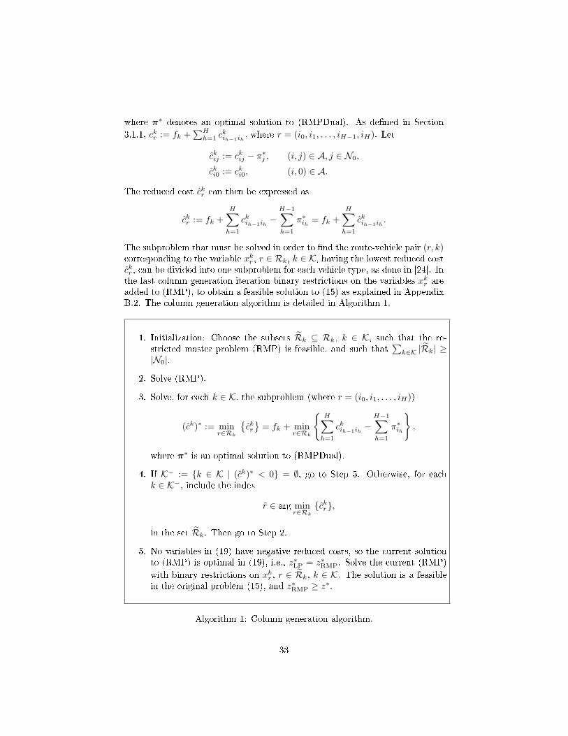
The subproblem that must be solved in order to �nd the route-vehicle pair (r, k)corresponding to the variable xkr , r ∈ Rk, k ∈ K, having the lowest reduced costckr , can be divided into one subproblem for each vehicle type, as done in [24]. Inthe last column generation iteration binary restrictions on the variables xkr areadded to (RMP), to obtain a feasible solution to (15) as explained in AppendixB.2. The column generation algorithm is detailed in Algorithm 1.
1. Initialization: Choose the subsets Rk ⊆ Rk, k ∈ K, such that the re-stricted master problem (RMP) is feasible, and such that
∑k∈K |Rk| ≥
|N0|.
2. Solve (RMP).
3. Solve, for each k ∈ K, the subproblem (where r = (i0, i1, . . . , iH))
(ck)∗ := minr∈Rk
{ckr}
= fk + minr∈Rk
{H∑h=1
ckih−1ih−H−1∑h=1
π∗ih
},
where π∗ is an optimal solution to (RMPDual).
4. If K− := {k ∈ K | (ck)∗ < 0} = ∅, go to Step 5. Otherwise, for eachk ∈ K−, include the index
r ∈ arg minr∈Rk
{ckr},
in the set Rk. Then go to Step 2.
5. No variables in (19) have negative reduced costs, so the current solutionto (RMP) is optimal in (19), i.e., z∗LP = z∗RMP. Solve the current (RMP)
with binary restrictions on xkr , r ∈ Rk, k ∈ K. The solution is a feasiblein the original problem (15), and z∗RMP ≥ z∗.
Algorithm 1: Column generation algorithm.
33
We have implemented some modi�cations of Algorithm 1 in order to speedup the convergence to the optimal value of (19). It is not necessary to solve thecolumn generation subproblem(s) to optimality, except for in the last iteration,when verifying that the solution to (RMP) is optimal in the complete master
problem (19); (see [8, 30]). Therefore, a route r ∈ Rk\Rk, such that the variablexkr has a negative but not necessarily minimal reduced cost ckr = ckr−
∑i∈N0
π∗i δkir
can be added to Rk in Step 4. In addition, since the original subproblem to �nda variable xkr with minimal reduced cost has been divided into one subproblemfor each vehicle type k, it is not necessary to solve the subproblem for everyvehicle type every iteration. Instead a so called partial column generation canbe employed, such that only a subset of the subproblems are considered eachiteration. However, at least one variable xkr with a negative reduced cost mustbe added to (RMP), provided that such a variable exists ([8]). Since there areas many subproblems as there are vehicle types, and the set of vehicle typesis assumed to be very large, using partial column generation can be bene�cial.Details on the solution of the subproblems are presented in Section 4.1.1.
In Section 4.1.2, upper and lower bounds, z and z, on z∗LP are derived.Since z∗LP is a lower bound on z∗, z is also a lower bound on z∗. The upperand lower bounds can be used to terminate the column generation prior to hasconvergence, i.e., when z−z ≤ ε, for some pre-determined value ε > 0. Whenthe column generation algorithm has converged, i.e., when the optimal solutionto the restricted master problem (RMP) has been veri�ed as an optimal solutionto the complete master problem (19), then it holds that z = z∗LP = z.
4.1.1 Subproblem
For a �xed value of k ∈ K, the column generation subproblem to �nd
(ck)∗ := minr∈Rk
{ckr}
= minr∈Rk
{ckr −
∑i∈N0
π∗i δkir
}= fk + min
r∈Rk
{H∑h=1
ckih−1ih
}(22)
is an elementary shortest path problem with resource constraints, since for k ∈ Kthe set Rk consist of elementary routes r = (i0, i1, . . . , iH−1, iH), starting and
ending at the depot, and that must satisfy∑H−1h=1 dih ≤ Dk (i.e., the total
demand of the customer nodes visited by route r can not be greater than thecapacity of vehicle k).
Two di�erent approaches have been used to solve (22) in this thesis, one us-ing AMPL and CPLEX, and one using dynamic programming in Matlab. Bothapproaches have been implemented in such a way that the solution algorithmcan be interrupted before an optimal solution to the subproblem has been found,either when a prede�ned time limit has been exceeded, or after a certain numberof routes with negative reduced cost has been found. It was noted that oftenwhen no route with negative reduced cost had been found for a given subproblemin the later iterations, then no route with negative reduced cost was found in thenext couple of iterations. Therefore, a kind of tabu-strategy of partial column
34
generation was also implemented for the subproblems (see [31] for an introduc-tion to tabu search), according to the following. If, for one speci�c subproblem,no routes with negative reduced cost have been found during a pre-determinednumber of consecutive column generation iterations, that speci�c subproblem isnot solved for a pre-determined number of iterations. When the extended testinstances CT12EXT were used, it was also noted that subproblems correspond-ing to vehicles with similar capacities sometimes yielded the same routes�bothwhen solved to optimality and when not. The tabu-strategy was then updated,so that only the route-vehicle pair with the lowest reduced cost was added to therestricted master problem, and the other subproblems which yielded the sameroute were recorded as not providing a route with negative reduced cost�thuspotentially leading to them not being solved for a number of iterations.
Mathematical formulations implemented in AMPL and CPLEX:
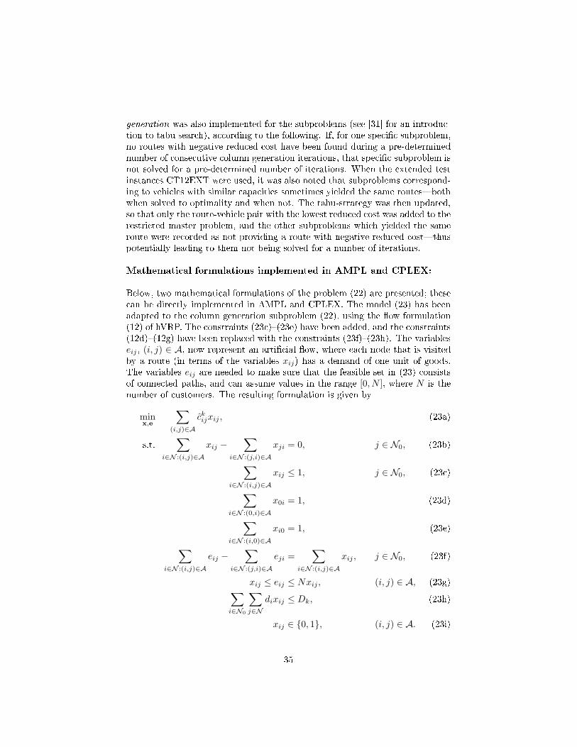
Below, two mathematical formulations of the problem (22) are presented; thesecan be directly implemented in AMPL and CPLEX. The model (23) has beenadapted to the column generation subproblem (22), using the �ow formulation(12) of hVRP. The constraints (23c)�(23e) have been added, and the constraints(12d)�(12g) have been replaced with the constraints (23f)�(23h). The variableseij , (i, j) ∈ A, now represent an arti�cial �ow, where each node that is visitedby a route (in terms of the variables xij) has a demand of one unit of goods.The variables eij are needed to make sure that the feasible set in (23) consistsof connected paths, and can assume values in the range [0, N ], where N is thenumber of customers. The resulting formulation is given by
minx,e
∑(i,j)∈A
ckijxij , (23a)
s.t.∑
i∈N :(i,j)∈A
xij −∑
i∈N :(j,i)∈A
xji = 0, j ∈ N0, (23b)
∑i∈N :(i,j)∈A
xij ≤ 1, j ∈ N0, (23c)
∑i∈N :(0,i)∈A
x0i = 1, (23d)
∑i∈N :(i,0)∈A
xi0 = 1, (23e)
∑i∈N :(i,j)∈A
eij −∑
i∈N :(j,i)∈A
eji =∑
i∈N :(i,j)∈A
xij , j ∈ N0, (23f)
xij ≤ eij ≤ Nxij , (i, j) ∈ A, (23g)∑i∈N0
∑j∈N
dixij ≤ Dk, (23h)
xij ∈ {0, 1}, (i, j) ∈ A. (23i)
35

The objective (23a) is to minimize the reduced route costs cij only, since the�xed cost fk will be present in any route. The constraints (23b) ensure thatthe vehicle departs from each customer that it arrives at. The constraints (23c)states that a customer may be visited at most once, while the constraints (23d)�(23e) ensure that at least one customer is visited. The constraints (23f)�(23g)are arti�cial constraints that are needed to make sure that the route is con-nected. Since the constraints (23f) should hold for all the customer nodes (i.e.N0), only cycles (with respect to the variables xij) that include the depot arefeasible, and the highest value taken by any variable eij , (i, j) ∈ A, will be e0j ,for the unique arc (0, j) ∈ A for which x0j = 1. The constraints (23h) imposethe vehicle capacity restrictions. For x∗ being an optimal solution to the model(23), we have that (ck)∗ = fk +
∑(i,j)∈A c
kijx∗ij .
We have adapted the formulation of the VRP with wime windows [32, p.58]�which employs variables representing time instead of �ow variables�for thecolumn generation subproblem (22). Here the variables eij and the constraints(23f)�(23g) are replaced by the variables si, i ∈ N , (representing order withrespect to time) and
si + 1 ≤ sj +N(1− xij), i ∈ N , j ∈ N0 : (i, j) ∈ A, (24a)
0 ≤ si ≤ N, i ∈ N , (24b)
resulting in the formulation (23a)�(23e), (23h)�(23i), (24). These constraintsare analogous to modelling very large time-windows, which are not restrictivein the sense that they do not cut away any solution that is feasible (the time-windows are [0, N ] for each customer node, where N is the number of customers,and it takes 1 time-unit to cross each arc in the networkA). The constraints (24)ensure that the resulting feasible set consists of connected elementary routes.The time variables si are fewer than the �ow variables eij ; their use may there-fore lead to a better formulation. Further, the alternative constraints make theconstraints (23c) redundant; they are not included in the formulation in [32, p.58]. However, they strengthen the formulation (in terms of a tighter represen-tation of the convex hull of the set of feasible solutions) and�according to thefollowing paragraph� yield great improvements in solution time when appliedto the subproblem (22).
The formulations (23) and (23a)�(23e), (23h)�(23i), (24) have been solved byAMPL and CPLEX. Our preliminary tests indicated that the two formulationsare rather similar with respect to solution time, although the latter formulationwith constraints (23c) removed is a lot more time-consuming�see Section 5.1.3.
Dynamic programming:
Instead of formulating integer linear programming models that can be solvedby AMPL and CPLEX, more e�cient solution methods, speci�cally tailored forshortest path problems with resource constraints, can be applied. Dynamic pro-gramming algorithms are especially suited for column generation subproblemsarising from vehicle routing problems, as discussed in Section 2.2. Solving the
36

subproblem (22), for a speci�c vehicle k using dynamic programming methodscan be done as in Algorithm 2.
1. Initialization: Let PNPP := {(1)}, PPP := ∅, PFP := ∅.
2. Pick one path P1i from the set PNPP of non-processed paths and extend itto all nodes j ∈ N0 for which (P1i, j) is a feasible path (a path is feasibleif the total demand of all nodes visited is not greater than the capacity ofthe vehicle (i.e., resource feasible) and no customer node has been visitedmore than once (i.e., the path is elementary)).
3. Find paths in PNPP ∪ PPP that are dominated by, or that dominates theextended paths from Step 2. Remove the dominated paths from theirrespective sets. Include the extended paths that were not dominated byany path in PNPP∪PPP in PNPP, and include the path P1i in the set PPP
of processed paths.
4. Extend the path P1i to include the depot, and include it in the set PFP
of full paths, if it has a lower objective value than all paths in PFP.
5. If PNPP = ∅, an optimal route is found in PFP, and the algorithm termi-nates. Otherwise, go to Step 2. Alternatively: Terminate the algorithmwhen a time limit has been exceeded, or when a pre-determined numberof paths have been processed.
Algorithm 2: Dynamic programming algorithm for the column generation sub-problem.
Since the subproblems (22) do not have to be solved to optimality in everyiteration of the column generation algorithm, Algorithm 2 may be terminatedbefore PNPP is empty. The dynamic programming algorithm is allowed to ter-minate when a full path with a negative reduced cost that is lower than somegiven threshold is found, and/or when a time limit has been exceeded. It isoften the case that an optimal route is found, but not veri�ed, early in the so-lution course. Terminating the algorithm before optimality is veri�ed may thensubstantially lower the solution time for the column generation.
The path P1i ∈ PNPP to be extended in Step 2 can be chosen accordingto di�erent criteria. Our implementation chooses the path having the lowestobjective value. Also, paths that can not be extended to any customer nodes,i.e., paths for which the sum of the demand of its visited customers exceeds thevalue (Dk − mini∈N0 di), are processed in Step 4 instead of being included inPNPP.
In Step 3, the domination criterion in Claim 1 (Section 2.2.1) is used. Hence,path P1i dominates path P ∗1i if (i) the sum of the customer demands of the nodesvisited by path P1i is less than or equal to that of P ∗1i, (ii) the cost of P1i is less
37
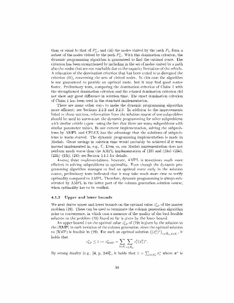
than or equal to that of P ∗1i, and (iii) the nodes visited by the path P1i form asubset of the nodes visited by the path P ∗1i. With this domination criterion, thedynamic programming algorithm is guaranteed to �nd the optimal route. Thecriterion has been strengthened by including in the set of nodes visited by a pathalso the nodes that are not reachable due to the capacity limitation of the vehicle.A relaxation of the domination criterion that has been tested is to disregard thecriterion (iii), concerning the sets of visited nodes. In this case the algorithmis not guaranteed to provide an optimal route, but it may �nd good routesfaster. Preliminary tests, comparing the domination criterion of Claim 1 withthe strengthened domination criterion and the relaxed domination criterion didnot show any great di�erence in solution time. The exact domination criterionof Claim 1 has been used in the standard implementation.
There are many other ways to make the dynamic programming algorithmmore e�cient; see Sections 2.2.2 and 2.2.3. In addition to the improvementslisted in those sections, information from the solution course of one subproblemshould be used to warm-start the dynamic programming for other subproblemswith similar vehicle types�using the fact that there are many subproblems withsimilar parameter values. In our current implementation, solving the subprob-lems by AMPL and CPLEX has the advantage that the solutions of subprob-lems is warm-started. The dynamic programming implementation is made inMatlab. Great savings in solution time would probably be achieved if it wereinstead implemented in, e.g., C. Even so, our Matlab implementation does notperform much worse than the AMPL implementation of (23) and (23a)�(23e),(23h)�(23i), (24); see Section 5.1.1 for details.
Among these implementations, however, AMPL is sometimes much moree�cient in solving subproblems to optimality. Even though the dynamic pro-gramming algorithm manages to �nd an optimal route early in the solutioncourse, preliminary tests indicated that it may take much more time to verifyoptimality compared to AMPL. Therefore, dynamic programming is always sub-stituted by AMPL in the latter part of the column generation solution course,when optimality has to be veri�ed.
4.1.2 Upper and lower bounds
We next derive upper and lower bounds on the optimal value z∗LP of the masterproblem (19). These can be used to terminate the column generation algorithmprior to convergence, in which case a measure of the quality of the best feasiblesolution to the problem (19) found so far is given by the lower bound.
An upper bound z on the optimal value z∗LP of (19) is given by the solution tothe (RMP) in each iteration of the column generation, since the optimal solutionto (RMP) is feasible in (19). For such an optimal solution
((xkr )∗
)r∈ eRk,k∈K
, it
holds thatz∗LP ≤ z := z∗RMP =
∑k∈K
∑r∈ eRk
ckr (xkr )∗.
By strong duality (e.g., [4, p. 248]), it holds that z =∑i∈N0
π∗i where π∗ is
38

optimal in (RMPDual) ([8]).The following reasoning provides a lower bound on z∗LP. Given an optimal
solution((xkr )∗
)r∈Rk,k∈K
to (19), it holds that
z∗LP − z =∑k∈K
∑r∈Rk
ckr (xkr )∗ −∑i∈N0
π∗i .
Since it holds that∑k∈K
∑r∈Rk
δkir(xkr )∗ = 1, i ∈ N0, we have that
z∗LP − z =∑k∈K
∑r∈Rk
ckr (xkr )∗ −∑i∈N0
(∑k∈K
∑r∈Rk
δkir(xkr )∗)π∗i
=∑k∈K
∑r∈Rk
(ckr −
∑i∈N0
δkirπ∗i
)(xkr )∗
≥
(∑k∈K
∑r∈Rk
(xkr )∗)c,
where c := minr∈Rk,k∈K{ckr −
∑i∈N0
δkirπ∗i
}is the lowest reduced cost over all
indices r ∈ Rk and k ∈ K, which is found by solving subproblem (22) for allk ∈ K. Since it holds that
∑k∈K
∑r∈Rk
(xkr )∗ ≤ |N0|, and c ≤ 0 it follows that
z∗LP − z ≥ c |N0|.
Hence a lower bound on z∗LP is given by z := c |N0| + z. This implies that thecolumn generation can be terminated when c is small enough, since c |N0| ≤ εand ε > 0 implies that z−z ≤ ε.
The result that z∗LP ≥ κ c+ z, where κ ≥∑k∈K
∑r∈Rk
(xkr )∗ is given withoutproof in [8]. A derivation of the lower bound z, similar to the one above, is foundin [9, Chapter 3.7] for κ = 1.
4.2 The restricted model with Benders' decomposition and
column generation
We next present a model for the many-hVRP, which is an alternative to thestraightforward model (cf. (15)) presented in Section 4.1. We have formulatedthis model for the many-hVRP; to the best of our knowledge it has not pre-viously been used for hVRP. In this new formulation, a constraint is added to(15) limiting the number of vehicle types that can be used. This is intended tomake the model more �exible, since in some applications a �eet with a limitednumber of vehicle types is to prefer. The constraint is also intended to allow fora Benders' decomposition of the problem. The new model is called the restrictedmodel.
De�ne the parameters M = the allowed number of vehicles of each type,and C = the allowed number of di�erent vehicle types, denoted the vehicle type
39

limit, and the variables
yk :=
{1, if vehicle type k is allowed,
0, otherwise,k ∈ K
The restricted model is then given by
minx,y
∑k∈K
∑r∈Rk
ckrxkr , (25a)
s.t.∑k∈K
∑r∈Rk
δkirxkr = 1, i ∈ N0, (25b)
∑r∈Rk
xkr ≤Myk, k ∈ K, (25c)
∑k∈K
yk ≤ C, (25d)
xkr ∈ {0, 1}, r ∈ Rk, k ∈ K, (25e)
yk ∈ {0, 1}, k ∈ K. (25f)
The di�erence between the formulation (25) and (15), is that the constraints(25c)�(25d) and the binary variables yk, k ∈ K, have been added; the constraints(25c) limit the number of vehicles of each type, and the constraint (25d) setsa limit on the number of di�erent vehicle types that may be used. If the for-mulation (25) and the formulation (15) share an optimal solution, for a speci�cproblem instance, then the vehicle type limit C is said to be non-restrictive.
4.2.1 Outline of Benders' decomposition applied to the restricted
model
To use Benders' decomposition, the binary requirements on the variables xkr arerelaxed, resulting in the following formulation9
v∗ := minx,y
∑k∈K
∑r∈Rk
ckrxkr , (26a)
s.t.∑k∈K
∑r∈Rk
δkirxkr = 1, i ∈ N0, (26b)
∑r∈Rk
xkr ≤Myk, k ∈ K, (26c)
∑k∈K
yk ≤ C, (26d)
xkr ≥ 0, r ∈ Rk, k ∈ K, (26e)
yk ∈ {0, 1}, k ∈ K. (26f)
9If the formulation (26) and the formulation (19) share an optimal solution for a speci�cproblem instance, then the vehicle type limit C is also said to be non-restrictive.
40

In model (26), the variables yk, k ∈ K are considered complicating. De�ne theset
R :=
(yk)Kk=1 ∈ {0, 1}K∣∣∣∣∣∣∑k∈K
yk ≤ C,∑
k∈Kcapacity
yk ≥ 1
,
for Kcapacity := {k ∈ K | Dk ≥ maxi∈N0{di}}. The set Kcapacity consists ofthose vehicle types k that can service all customers, thus the set R consists ofthose variable values of the complicating variables y for which the remainingproblem (26), in the variables x, has at least one feasible solution.
When applying Benders' decomposition to (26) (see Section 2.3) the Benderssubproblem for �xed values of the variables y := (yk)k∈K appears as
(BendersSP(y)) w∗(y) := minx,y
∑k∈K
∑r∈Rk
ckrxkr ,
s.t.∑k∈K
∑r∈Rk
δkirxkr = 1, i ∈ N0,∑
r∈Rk
xkr ≤Myk, k ∈ K,
xkr ≥ 0, r ∈ Rk, k ∈ K,
and the corresponding dual problem is given by
(BendersSPDual(y)) maxπ,γ
(∑i∈N0
πi +∑k∈K
Mykγk
), (27a)
s.t.∑i∈N0
πiδkir + γk ≤ ckr , r ∈ Rk, k ∈ K, (27b)
γk ≤ 0, k ∈ K. (27c)
We denote the feasible set (corresponding to the feasible set de�ned by theconstraints (8b)�(8c) in Section 2.3)
FBendersSPDual :={
(π,γ) ∈ R|N0|+|K|∣∣∣ (π,γ) satis�es (27b)�(27c)
}.
De�ning the constrained set of vehicles as K(y) := {k ∈ K | yk = 1}, anequivalent formulation to (BendersSP(y)) is
minx
∑k∈eK(ey)
∑r∈Rk
ckrxkr , (28a)
s.t.∑
k∈K(ey)
∑r∈Rk
δkirxkr = 1, i ∈ N0, (28b)
∑r∈Rk
xkr ≤M, k ∈ K(y), (28c)
xkr ≥ 0, r ∈ Rk, k ∈ K(y). (28d)
41

If M is chosen large enough (e.g., M = |N0|), then the constraints (28c) arenot restrictive and can be removed from this formulation. We assume from nowon that M has been chosen so that it is not restrictive. The models (28) and(19) are thus equivalent, except that the set of allowed vehicle types is smallerin the former, and Algorithm 1 can be applied to �nd an optimal solution to(28a)�(28b), (28d) (which will give an optimal solution to (BendersSP(y)) bysetting xkr := 0, r ∈ Rk, k ∈ K \ K(y)).
Each time the subproblem (BendersSP(y)) is solved, we seek an optimalextreme point (π∗,γ∗) to (BendersSPDual(y)). How to �nd such an optimalextreme point is detailed in Section 4.2.2. Let L denote the current Bendersiteration, and let L := {1, . . . , L−1} be the set of previous iterations. The dualsolution (πL,γL) := (π∗,γ∗) de�nes a new constraint
v ≥∑i∈N0
πLi +∑k∈K
MykγLk , (29)
to be added to Benders restricted master problem, which is given by
(BendersRMP) v∗ := minv,y
v,
s.t. v ≥∑i∈N0
πli +∑k∈K
Mykγlk, l ∈ L,
y ∈ R.
After adding the new constraint (29) to (BendersRMP) it is solved for op-timal values (vL, yL). This de�nes the new problems (BendersSP(yL)) and(BendersSPDual(yL)), which are solved to generate a new constraint (29) to(BendersRMP). This process is iterated�adding one constraint (29) in eachBenders iteration�until an optimal solution to (26) is found and veri�ed. Howto determine that such an optimal solution has been found, and the resultingBenders' algorithm, is described in Section 4.2.3. Note that (BendersRMP),(BendersSP(y)), and (BendersSPDual(y)), correspond to the general problems,(10), (7), and (8), respectively, in Section 2.3.
4.2.2 Optimal extreme point to Benders subproblem
Since it is the compact formulation (28a)�(28b), (28d) that is solved each Ben-ders iteration, and not the equivalent problem (BendersSP(y)), some extra e�orthas to be put into �nding an extreme point of the feasible set FBendersSPDualthat is optimal in the dual (27) of (BendersSP(y)). To this end, Claims 2 and3 have been formulated and proven.
The �nal column generation iteration in the solution course for the model(28a)�(28b), (28d), results in optimal dual variable values π which are optimal
42
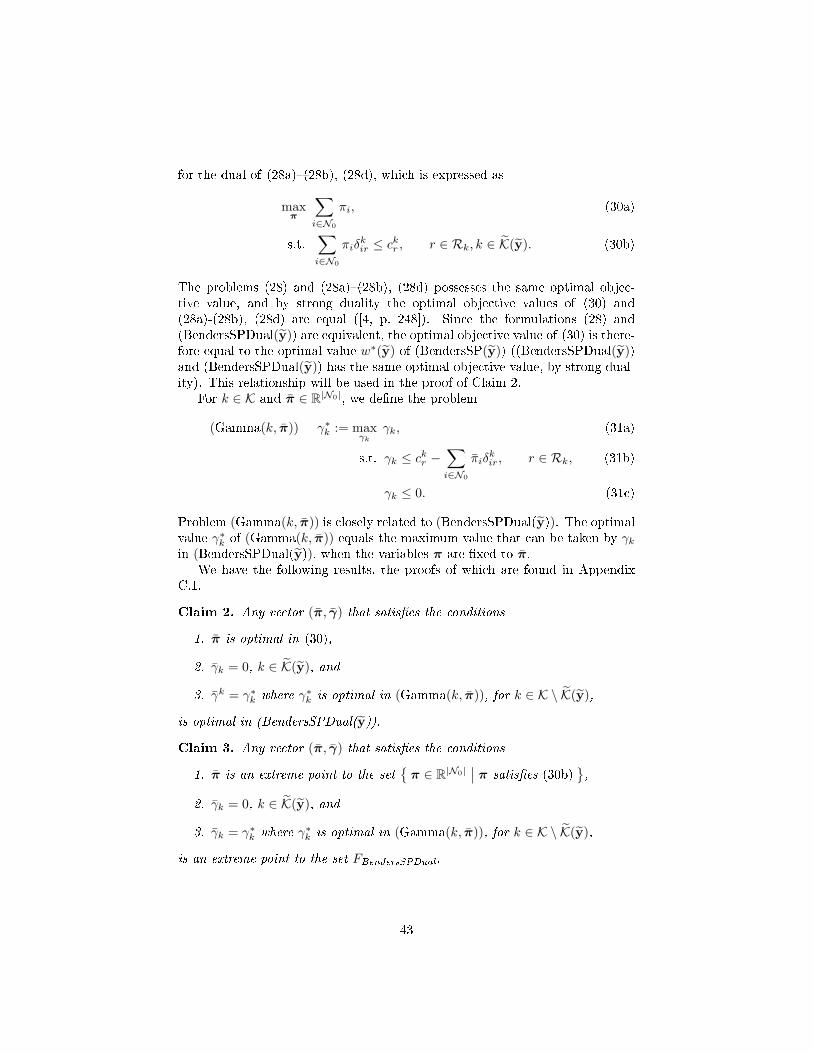
for the dual of (28a)�(28b), (28d), which is expressed as
maxπ
∑i∈N0
πi, (30a)
s.t.∑i∈N0
πiδkir ≤ ckr , r ∈ Rk, k ∈ K(y). (30b)
The problems (28) and (28a)�(28b), (28d) possesses the same optimal objec-tive value, and by strong duality the optimal objective values of (30) and(28a)-(28b), (28d) are equal ([4, p. 248]). Since the formulations (28) and(BendersSPDual(y)) are equivalent, the optimal objective value of (30) is there-fore equal to the optimal value w∗(y) of (BendersSP(y)) ((BendersSPDual(y))and (BendersSPDual(y)) has the same optimal objective value, by strong dual-ity). This relationship will be used in the proof of Claim 2.
For k ∈ K and π ∈ R|N0|, we de�ne the problem
(Gamma(k, π)) γ∗k := maxγk
γk, (31a)
s.t. γk ≤ ckr −∑i∈N0
πiδkir, r ∈ Rk, (31b)
γk ≤ 0. (31c)
Problem (Gamma(k, π)) is closely related to (BendersSPDual(y)). The optimalvalue γ∗k of (Gamma(k, π)) equals the maximum value that can be taken by γkin (BendersSPDual(y)), when the variables π are �xed to π.
We have the following results, the proofs of which are found in AppendixC.1.
Claim 2. Any vector (π, γ) that satis�es the conditions
1. π is optimal in (30),
2. γk = 0, k ∈ K(y), and
3. γk = γ∗k where γ∗k is optimal in (Gamma(k, π)), for k ∈ K \ K(y),
is optimal in (BendersSPDual(y)).
Claim 3. Any vector (π, γ) that satis�es the conditions
1. π is an extreme point to the set{π ∈ R|N0|
∣∣ π satis�es (30b)},
2. γk = 0, k ∈ K(y), and
3. γk = γ∗k where γ∗k is optimal in (Gamma(k, π)), for k ∈ K \ K(y),
is an extreme point to the set FBendersSPDual.
43

After solving (28a)�(28b), (28d)�the solution of which is optimal in Ben-ders subproblem (BendersSP(y)), where the excluded variables are set to zero
(xkr := 0, r ∈ Rk, k ∈ K \ K(y))�using column generation, a value of π sat-isfying condition 1 of Claim 2 results from the last iteration. The importantconsequences of Claims 2 and 3 are the following: if γ satis�es conditions 2 and3 of Claim 2, then (π, γ) is optimal in (BendersSPDual(y)). If π also satis�escondition 1 of Claim 3�making π an optimal extreme point to (30)�and γsatis�es conditions 2 and 3 of Claim 2 (and consequently also of Claim 3) forthe chosen value of π, then (π, γ) is an extreme point to FBendersSPDual that isoptimal in (BendersSPDual(y)).
Notice that the variable values γ = (γk)k∈K, that satisfy conditions 2 and
3 of Claim 2, are given by γk = min{
0,minr∈Rk
{ckr}}
(where γk is the opti-mal solution value of (Gamma(k, π))). In the context of the linear relaxation(19) of the straightforward model, ckr is the reduced cost of variable xkr (com-pare (31) with the reduced cost (21)). Hence, γk has the interpretation of thechange in objective value relative to the optimal solution to Benders subprob-lem (BendersSP(y)) that would be achieved, if the route-vehicle pair corre-sponding to the variable xkr�with minimal reduced cost among the variablesxkr , r ∈ Rk�was allowed in a solution to Benders subproblem (and the valueof xkr is increased by one, moving in the direction of a particular neighbouringextreme point)10. Interestingly, the right-hand side of each constraint (29) thatis added to (BendersRMP) according to Claim 2, is the sum of
∑i∈N0
πLi (whichequals the optimal objective value of Benders subproblem in Benders iterationL) and
∑k∈KMykγLk (being the sum of scaled �minimal reduced costs�, γLk , from
Benders iteration L, for all vehicle types in the set {k ∈ K | yk = 1} =: K(y)).
4.2.3 Benders' algorithm
With (v∗, y∗) optimal in (BendersRMP), x∗ optimal in (BendersSP(y∗)), and(π∗,γ∗) optimal in (BendersSPDual(y∗)), we have that (x∗, y∗) must be anoptimal solution to (26) if it holds that
v∗ =∑i∈N0
π∗i +∑k∈K
M(yk)∗γ∗k . (32)
This, since v∗ is a lower bound on the optimal value v∗ of (26), and∑i∈N0
π∗i +∑k∈KM(yk)∗γ∗k =
∑k∈K
∑r∈Rk
ckr (xkr )∗ = w∗(y∗) is an upper bound on v∗.If the equation (32) does not hold,the following inequality
v∗ <∑i∈N0
π∗i +∑k∈K
M(yk)∗γ∗k , (33)
10Similarly to how the reduced cost in the context of the column generation algorithmmeasures the change in objective value relative to the current optimal solution value of thecolumn generation RMP, if the corresonding variable is allowed; see Section 2.1 and AppendixB.1.
44

must hold. Thus, adding to (BendersRMP) the constraint v ≥∑i∈N0
π∗i +∑k∈KMykγ∗k , would make the current solution (v∗, y∗) infeasible.Following the procedure described in Section 2.3, Benders' algorithm itera-
tively solves (BendersRMP) for (v∗, y∗) and (BendersSPDual(y∗)) for (π∗,γ∗)�each iteration adding a constraint to (BendersRMP)�until an optimal solutionto (26) is found and veri�ed, i.e., until the equation (32) holds. Benders' algo-rithm for the restricted model (25) is outlined in Algorithm 3.
1. Initialization: Choose y1 ∈ R and solve (BendersSP(y1)) for (π1,γ1),de�ning the �rst constraint,
v ≥∑i∈N0
π1i +
∑k∈K
Mykγ1k,
of (BendersRMP).
2. Solve (BendersRMP) for (vL, yL).
3. For xL, solve (BendersSP(yL)) by solving (28a)�(28b), (28d) using columngeneration. In the last column generation, add binary restrictions onthe variables xrk, r ∈ Rk, k ∈ K, and �nd a solution xLbinary, such that
(yL, xLbinary) is feasible in (25).
4. If w∗(yL) > vL, �nd an extreme point (πL,γL) that is optimal in(BendersSPDual(yL)), by using an optimal extreme point π to (30)�the dual of (28a)�(28b), (28d)�as prescribed in Claims 2 and 3. Add thenew constraint
v ≥∑i∈N0
πLi +∑k∈K
MykγLk ,
to (BendersRMP) and go to Step 2. Otherwise w∗(yL) = vL = v∗; hence(yL, xL) is optimal in (26). Terminate the algorithm.
Algorithm 3: Benders' decomposition algorithm.
A lower bound on the optimal value v∗ of the problem (26) is given in eachBenders iteration by vL. This lower bound is non-decreasing. An upper boundon v∗ is given in each Benders iteration by the optimal objective value w∗(yL)of Benders subproblem (BendersSP(yL)). This upper bound is, however, notnon-increasing. A better upper bound, which is non-increasing, is given byminl∈{1,...,L}
{w∗(yl)
}([33]). Since the optimality condition (32) (which is the
termination criterion that has been implemented) is equivalent to vL = w∗(yL),this implies that a stronger optimality condition would be given by
vL = minl∈{1,...,L}
{w∗(yl)
}. (34)
45

Benders' algorithm could be set to terminate when minl∈{1,...,L}{w∗(yl)
}−
vL ≤ ε, for some ε > 0, since then the di�erence between the best feasible solu-tion that has been found so far�with the objective value minl∈{1,...,L}
{w∗(yl)
}�
and an optimal solution to (26)�with the objective value v∗�is not greater thanε.
Since Benders' algorithm is applied to the relaxation (26) of the restrictedmodel (25), v∗ (and thus also vL) is only a lower bound on the optimal value of(25). An upper bound is given in Benders iteration L by the smallest objectivevalue in (25) of the feasible solutions (yl, xlbinary), l = 1, . . . , L.
It may not necessarily be the case that Benders' algorithm terminates when(xL, yL) optimal in (26) are found. This has not been proven, but an intuitiveargument for why optimality would not be veri�ed is the following: if all con-straints (29) that are binding in the optimal solution have not been generatedin Benders iteration L, it may happen that vL < v∗, even if yL is an optimalchoice of variable values in (26), i.e., even if w∗(yL) = v∗.
However, Algorithm 3 will converge after a �nite number of iterations, if, ineach Benders iteration L, the optimal solution (πL,γL) is chosen as an extremepoint to the feasible set FBendersSPDual of (BendersSPDual(yL)). The set Rde�ning the set of feasible values for y in (BendersRMP) is �nite, thus there isonly a �nite number of possible problems (BendersSPDual(y)), for each of whichan optimal extreme point can be found for each (BendersSPDual(y)). If for twodistinct Benders iterations, l1 and l2, it holds that yl1 = yl2 , then the optimalitycriterion (32) is ful�lled, and since the set R is �nite, �nite convergence follows.The same result should hold, also if a solution (πL,γL) that is optimal but notnecessarily an extreme point in (BendersSPDual(yL)) is chosen. This is just anintuitive argument, however.
An argument for the �nite convergence of Algorithm 3 can be based on theproof of �nite convergence for a generalized Benders' decomposition found in[34, Theorem 6.3.4, p 125]. The argument for the general Benders' algorithm, aspresented in Section 2.3, is that the algorithm is guaranteed to converge �nitelysince there is only a �nite number of extreme points to the feasible set of thedual of Benders subproblem [9].
With the proposed procedure for �nding (πL,γL) in Algorithm 3, it may bethe case that only one of possibly several optimal extreme points to the dual(BendersSPDual(yL)) can be found. Thus, we can not be sure that all extremepoints to FBendersSPDual can be found in the solution course of the proposedBenders' algorithm.
4.2.4 Additions to Benders' algorithm
To improve the speed of convergence of Algorithm 3, another step has beenimplemented, in which optimal solutions xl to (BendersSP(yl)), from previousiterations l = 1, . . . , L− 1 of Benders' algorithm, are tested to see if the corre-sponding routes would yield a better objective value when used in combinationwith other vehicles. This procedure is called projection of routes.
46
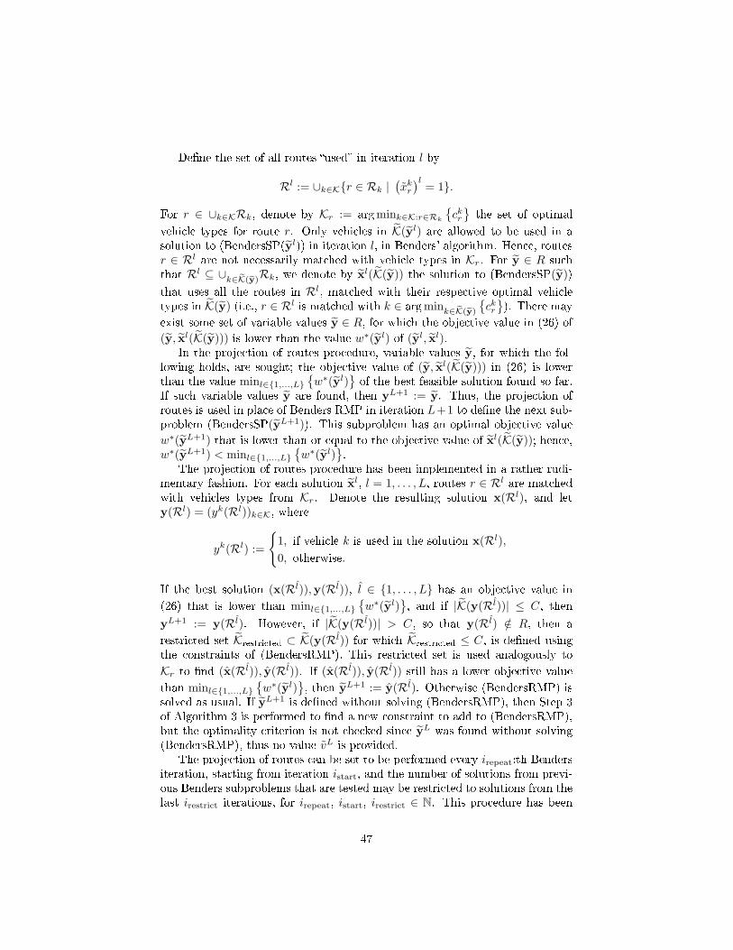
De�ne the set of all routes �used� in iteration l by
Rl := ∪k∈K{r ∈ Rk |(xkr)l
= 1}.
For r ∈ ∪k∈KRk, denote by Kr := argmink∈K:r∈Rk
{ckr}the set of optimal
vehicle types for route r. Only vehicles in K(yl) are allowed to be used in asolution to (BendersSP(yl)) in iteration l, in Benders' algorithm. Hence, routesr ∈ Rl are not necessarily matched with vehicle types in Kr. For y ∈ R suchthat Rl ⊆ ∪k∈eK(ey)Rk, we denote by xl(K(y)) the solution to (BendersSP(y))that uses all the routes in Rl, matched with their respective optimal vehicletypes in K(y) (i.e., r ∈ Rl is matched with k ∈ argmink∈eK(ey)
{ckr}). There may
exist some set of variable values y ∈ R, for which the objective value in (26) of
(y, xl(K(y))) is lower than the value w∗(yl) of (yl, xl).In the projection of routes procedure, variable values y, for which the fol-
lowing holds, are sought; the objective value of (y, xl(K(y))) in (26) is lowerthan the value minl∈{1,...,L}
{w∗(yl)
}of the best feasible solution found so far.
If such variable values y are found, then yL+1 := y. Thus, the projection ofroutes is used in place of Benders RMP in iteration L+1 to de�ne the next sub-problem (BendersSP(yL+1)). This subproblem has an optimal objective value
w∗(yL+1) that is lower than or equal to the objective value of xl(K(y)); hence,w∗(yL+1) < minl∈{1,...,L}
{w∗(yl)
}.
The projection of routes procedure has been implemented in a rather rudi-mentary fashion. For each solution xl, l = 1, . . . , L, routes r ∈ Rl are matchedwith vehicles types from Kr. Denote the resulting solution x(Rl), and lety(Rl) = (yk(Rl))k∈K, where
yk(Rl) :=
{1, if vehicle k is used in the solution x(Rl),0, otherwise.
If the best solution (x(Rl)),y(Rl)), l ∈ {1, . . . , L} has an objective value in
(26) that is lower than minl∈{1,...,L}{w∗(yl)
}, and if |K(y(Rl))| ≤ C, then
yL+1 := y(Rl). However, if |K(y(Rl))| > C, so that y(Rl) /∈ R, then a
restricted set Krestricted ⊂ K(y(Rl)) for which Krestricted ≤ C, is de�ned usingthe constraints of (BendersRMP). This restricted set is used analogously to
Kr to �nd (x(Rl)), y(Rl)). If (x(Rl)), y(Rl)) still has a lower objective value
than minl∈{1,...,L}{w∗(yl)
}, then yL+1 := y(Rl). Otherwise (BendersRMP) is
solved as usual. If yL+1 is de�ned without solving (BendersRMP), then Step 3of Algorithm 3 is performed to �nd a new constraint to add to (BendersRMP),but the optimality criterion is not checked since yL was found without solving(BendersRMP), thus no value vL is provided.
The projection of routes can be set to be performed every irepeat:th Bendersiteration, starting from iteration istart, and the number of solutions from previ-ous Benders subproblems that are tested may be restricted to solutions from thelast irestrict iterations, for irepeat, istart, irestrict ∈ N. This procedure has been
47

shown to greatly reduce the time before an optimal solution to (26) is found;see Section 5.2.3. Even greater improvements in solution time would proba-bly be achieved by improving this procedure of projecting routes, especially byimproving the handling of restrictive values of the vehicle type limit C.
To improve the solution speed of Benders subproblems, a so called warm startcan be utilized, according to the following. The routes ∪Ll=1Rl that are part ofthe previous optimal solutions to Benders subproblems, i.e., xl, l = 1, . . . , L, andwhich can be taken by some vehicle in the current Benders iteration�i.e., the
routes in the set(∪Ll=1Rl
)∩(∪k∈∪ eK(eyL+1)Rk
)�are included in the set of routes
used to start the column generation algorithm for solving Benders subproblemin iteration L+ 1. This has been shown to reduce the time spent in the columngeneration algorithm. It is even the case that in most iterations of Benders'algorithm, an optimal solution to Benders subproblem can be found among theroutes provided by the warm start. See Section 5.2.2 for details.
The projection of routes procedure and the warm start, described in thissection, use some ideas from the set-partitioning based heuristic for hVRP byTaillard ([20]), described in Section 3.1.2. In [20] each route r generated ina homogeneous VRP determines route-vehicle pairs (r, k) in a set-partitioningformulation for hVRP, for each vehicle type in the set {k ∈ K | r ∈ Rk}.
4.2.5 Suggestions for further improvements of Benders' algorithm
To get an optimal extreme point to FBendersSPDual, by Claims 2 and 3, Benderssubproblem should be solved to optimality using column generation to �nd anoptimal extreme point π to the problem (30). However, at the later iterationsof the column generation often very small improvements are made, known asthe tailing o� e�ect (see [8]). It is possible that good quality constraints of(BendersRMP) can be provided by using points in the set FBendersSPDual thatare not necessarily extreme points, or even non-optimal in the current Benderssubproblem. This, since for any (π,γ) ∈ FBendersSPDual, the inequality
v ≥∑i∈N0
πi +∑k∈K
Mykγk (35)
is a valid constraint in (BendersRMP) (see [35, p. 308]). Thus, the column gen-eration algorithm for Benders subproblem can be terminated before an optimalextreme point to (30) is found, and the variable values π that are optimal inthe dual of the current column generation RMP, can be used to de�ne a newconstraint�for any π ∈ R|N0| it holds that (π,γ) ∈ FBendersSPDual whenever itholds that γ := (γk)k∈K, γk ≤ γ∗k , and γ∗k is optimal in (Gamma(k,π)).
It follows that, instead of solving the problem (Gamma(k,π)), k ∈ K, ineach Benders iteration11 (as prescribed in Claim 2), lower bounds on the op-timal values of problems the (Gamma(k,π)), k ∈ K, can be used to de�ne a
11We investigated if it would be possible to �nd a set of conditions under which γ ∈argmin (Gamma(k1,π)) implies the inclusion γ ∈ argmin (Gamma(k2,π)), for k1 6= k2. Wedid not, however, �nd any such conditions; see Appendix C.2.
48
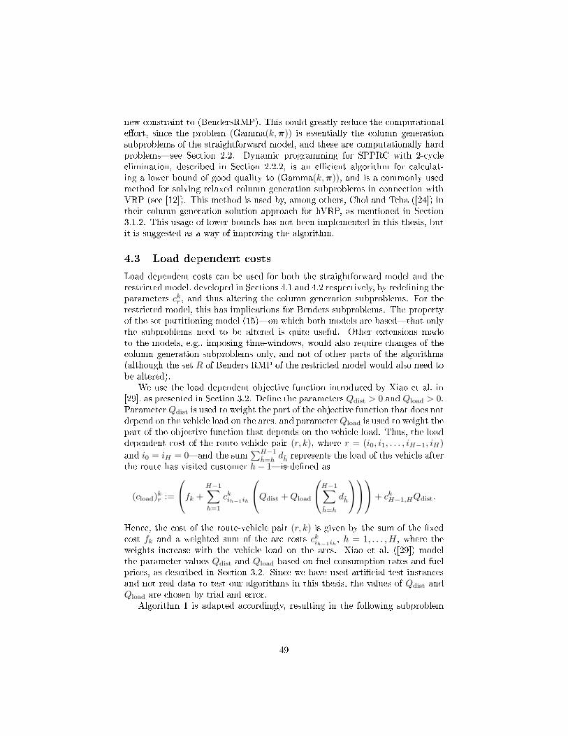
new constraint to (BendersRMP). This could greatly reduce the computationale�ort, since the problem (Gamma(k,π)) is essentially the column generationsubproblems of the straightforward model, and these are computationally hardproblems�see Section 2.2. Dynamic programming for SPPRC with 2-cycleelimination, described in Section 2.2.2, is an e�cient algorithm for calculat-ing a lower bound of good quality to (Gamma(k,π)), and is a commonly usedmethod for solving relaxed column generation subproblems in connection withVRP (see [12]). This method is used by, among others, Choi and Tcha ([24]) intheir column generation solution approach for hVRP, as mentioned in Section3.1.2. This usage of lower bounds has not been implemented in this thesis, butit is suggested as a way of improving the algorithm.
4.3 Load dependent costs
Load dependent costs can be used for both the straightforward model and therestricted model, developed in Sections 4.1 and 4.2 respectively, by rede�ning theparameters ckr , and thus altering the column generation subproblems. For therestricted model, this has implications for Benders subproblems. The propertyof the set-partitioning model (15)�on which both models are based�that onlythe subproblems need to be altered is quite useful. Other extensions madeto the models, e.g., imposing time-windows, would also require changes of thecolumn generation subproblems only, and not of other parts of the algorithms(although the set R of Benders RMP of the restricted model would also need tobe altered).
We use the load dependent objective function introduced by Xiao et al. in[29], as presented in Section 3.2. De�ne the parameters Qdist > 0 and Qload > 0.Parameter Qdist is used to weight the part of the objective function that does notdepend on the vehicle load on the arcs, and parameter Qload is used to weight thepart of the objective function that depends on the vehicle load. Thus, the loaddependent cost of the route-vehicle pair (r, k), where r = (i0, i1, . . . , iH−1, iH)and i0 = iH = 0�and the sum
∑H−1
h=hdh represents the load of the vehicle after
the route has visited customer h− 1�is de�ned as
(cload)kr :=
fk +H−1∑h=1
ckih−1ih
Qdist +Qload
H−1∑h=h
dh
+ ckH−1,HQdist.
Hence, the cost of the route-vehicle pair (r, k) is given by the sum of the �xedcost fk and a weighted sum of the arc costs ckih−1ih
, h = 1, . . . ,H, where theweights increase with the vehicle load on the arcs. Xiao et al. ([29]) modelthe parameter values Qdist and Qload based on fuel consumption rates and fuelprices, as described in Section 3.2. Since we have used arti�cial test instancesand not real data to test our algorithms in this thesis, the values of Qdist andQload are chosen by trial and error.
Algorithm 1 is adapted accordingly, resulting in the following subproblem
49

for k ∈ K:
minr∈Rk
(cload)kr = minr∈Rk
{(cload)kr −
∑i∈N0
π∗i δkir
}(36)
The same dynamic programming algorithm, i.e., Algorithm 2, that is used forthe standard column generation subproblems (22) can also be used for the sub-problems (36) by altering the caluclation of the cost for each path. The conditionin Claim 1 pertaining to the cost of each path can be modi�ed, with correspond-ing modi�cations of the proof, so that the claim holds also for the subproblems(36).
Of the two formulations (23) and (23a)�(23e), (23h)�(23i), (24) used for thestandard column generation subproblems (22), only the former can be used inthe case of load dependent costs (36) (with some alterations). Now the vari-ables eij , (i, j) ∈ A, instead of representing an arti�cial �ow�as in formulation(23)�represents the actual �ow of goods�as in formulation (12). The resultingsubproblem formulation used in this thesis, is given by
minx,e
∑(i,j)∈A
(ckij(Qdistxij +Qload eij)− π∗i xij
), (37a)
s.t.∑
i∈N :(i,j)∈A
xij −∑
i∈N :(j,i)∈A
xji = 0, j ∈ N0, (37b)
∑i∈N :(i,j)∈A
xij ≤ 1, j ∈ N0, (37c)
∑i∈N :(0,i)∈A
x0i = 1, (37d)
∑i∈N :(i,0)∈A
xi0 = 1, (37e)
∑i∈N :(i,j)∈A
eij −∑
i∈N :(j,i)∈A
eji = dj
∑i∈N :(i,j)∈A
xij
, j ∈ N0, (37f)
djxij ≤ eij ≤ (Dk − di)xij , (i, j) ∈ A, (37g)
xij ∈ {0, 1}, (i, j) ∈ A. (37h)
The objective (37a) is to minimize the reduced cost. The constraints (37b)�(37e)are equivalent to the constraints (23b)�(23e). The constraints (37f) have beenadapted from the constraints (12d), and the constraints (37g) are equivalent tothe constraints (13), reformulated for a homogeneous problem.
50

5 Tests and results
Both the straightforward and the restricted model has been tested on the original(CT12) and the extended (CT12EXT) test instances; the results are presentedin Sections 5.1 and 5.2, respectively. The latter of the instance sets�includingmore vehicle types than the former�are described in Section 3.1.3.
The test were performed on Linux computers with a Pentium Dual-CoreCPU 2.5 GHz with 2048 KB cache. The mathematical models and algorithmshave been implemented using the modelling software AMPL 12.1.0 ([36]), andthe optimization solver CPLEX 12 ([37]). Dynamic programming for the col-umn generation subproblems and some other calculations (e.g., �nding initialsolutions to the column generation RMP, and for warm start and projectionof routes in Benders' algorithm) have been implemented in Matlab 2012b [38].The communication between AMPL and Matlab is done via text �les. The bashcommand screen is used to enable a single Matlab session being opened andcalled several times from AMPL. Matlab has also been used for the visualizationof solutions and algorithm performance data.
5.1 The original test instances, CT12
The test instances CT12 have been used to test the column generation algorithm,implemented as described in Section 4.1. Since these instances contain only threeto six vehicle types, the corresponding tests of the column generation algorithmconcern the hVRP, not the many-hVRP.
In Section 5.1.1, the results from these tests are compared with the bestpublished results for hVRP on CT12, as well as with an implementation ofthe �ow formulation (12) solved directly by AMPL and CPLEX. In Sections5.1.2 and 5.1.3, tests of di�erent ways initializations of the column generationalgorithm and di�erent implementations of the algorithms (described in Section4.1.1) for the column generation subproblems, are presented.
5.1.1 Comparison of solution methods
In this section, the column generation applied to the model (15) (the straightfor-ward model of Section 4.1) is compared with a straightforward implementationof the �ow formulation (12), as well as with the results of Choi and Tcha in [24]and with the best known results for CT12. The column generation applied to(15), described in Section 4.1, has been implemented in AMPL and CPLEX,using Matlab with dynamic programming and/or AMPL and CPLEX for thecolumn generation subproblems (22). The �ow formulation (12) has been im-plemented in AMPL and CPLEX.
In Table 2 results for the �ow formulation (12) are presented. Table 5 showsthe results from the column generation algorithm by Choi and Tcha ([24]) (theseresults were obtained using a Pentium IV 2.6 GHz processor). Table 3 and 4 liststhe results from our standard implementation of column generation on CT12.The results in Table 3 were obtained using dynamic programming for the column
51

generation subproblems in the former part and AMPL and CPLEX in the latterpart of the solution course, whereas the results in Table 4 were obtained usingonly AMPL and CPLEX for the column generation subproblems. Both thesolve time�i.e. the CPU time spent in the column generation algorithm inAMPL and CPLEX, and the clock time spent in the dynamic programmingin Matlab for the column generation subproblems�and the total time�i.e.,the clock time from the algorithm is starts until it �nishes�are presented inthe tables. In addition to time spent in the column generation algorithm, thetotal time also includes the time spent calculating the heuristic solution usedto start the column generation, and the time spent in communications betweenAMPL/CPLEX and Matlab. The calculations were interrupted after 10000CPU seconds12. The lower bound z, was calculated after the column generationalgorithm was terminated (for some of the larger instances, these calculationswere aborted with an out-of-memory error). More details about the columngeneration implementation are presented in Sections 5.1.2 and 5.1.3.
In Tables 2�5, �Obj. value� refers to the objective value of the best feasiblesolution to (15) found, and �Opt. gap� = (�Obj. value� - zbestknown)/zbestknown,where zbestknown is the objective value of the best feasible solutions known forthe instances in CT12, (see [23, Table 7]).
Instance Obj. value LB Opt. gap [%]
Choi3 1154.8 986.1 0.89Choi4 6437.3 6281.7 0Choi5 1357.2 1027.8 2.64Choi6 7021.3 6310.8 7.75T13 3238.0 2401.6 9.22T14 9672.1 1034.8 5.97T15 2760.6 424.8 4.77T16 3524.1 843.5 11.21T17 2846.9 1190.8 42.03T18 4744.8 2449.5 50.72T19 10274.1 2110.6 18.61T20 4778.8 116.1 15.03
Table 2: Results from a straightforward implementation of the model (12) inAMPL. The computations were interrupted after 10000 CPU seconds. �LB�refers to the current lower bound provided by AMPL and CPLEX when thecomputations were interrupted.
12The column generation algorithm is set to terminate when the solve time exceeds 10000CPU seconds. The solve time is, however measured only at the start of each column generationiteration. This explains why the total solve time for T16 in Table 4 is 22810 CPU seconds�thesubproblems are solved to optimality after approximately 5000 CPU seconds, which leads tothe last column generation iteration (before the algorithm is terminated) taking approximately17000 CPU seconds.
52

Comparing the results from the column generation algorithm implementa-tions presented in Tables 3 and 4, using dynamic programming for the sub-problems in the �rst part of the column generation algorithm (Table 3) yieldsbetter objective values than when not using dynamic programming (Table 4).Comparing the best feasible solutions to (25) found, the column generation withdynamic programming found solutions with lower or equal objective values forall instances except Choi3. Comparing the upper bounds z on the optimal ob-jective value of (26) for the instances T14�T20 (for which the column generationdid not converge in 10000 CPU seconds), the column generation with dynamicprogramming provided upper bounds that were strictly lower for all instances ex-cept T14. For these reasons, the column generation with dynamic programmingfor the subproblems is set as the standard, even though the column generationwhere dynamic programming is not used converges faster.
Instance Obj. value z z TOPT TTOT Opt. gap[CPU s] [s] [%]
Choi3 1150.9 1139.8 1139.8 299 348 0.55Choi4 6484.9 6370.8 6370.8 691 747 0.74Choi5 1322.3 1308.4 1308.4 556 516 0Choi6 6524.4 6451.6 6451.6 765 779 0.12T13 2969.7 2959.8 2959.8 8107 5657 0.17T14∗ 12771.5 9311.0 < 0 10519 10743 39.93T15 2692.5 2608.8 2153.4 10139 8243 2.18T16 3210.1 3139.0 2286.3 10089 7989 1.30T17∗ 2556.8 2159.3 � 10134 10347 27.55T18 3249.1 3188.0 � 10282 10507 3.21T19∗ 12957.5 9743.4 � 10029 10348 49.59T20∗ 5659.2 4517.6 � 10145 10484 36.22
Table 3: Results from the column generation, implemented in AMPL and Mat-lab and using dynamic programming. ∗ indicates that no improvement of theinitial, heuristic solution was made, in the objective value �Obj. value� of thebest feasible solution to (15) found. z and z denote the upper and lower bound,respectively, de�ned in Section 4.1.2, of the optimal value, z∗LP, of the LP relax-ation (19). �TOPT� refers to the total solve time in AMPL/CPLEX and Matlab.�TTOT� refers to the total time of the whole algorithm.
Solving the �ow formulation directly in AMPL and CPLEX requires a verylong computing time. The calculations were interrupted after a pre-de�ned timelimit of 10000 CPU seconds, and for none of the test instances was an optimalsolution veri�ed. Comparing the results presented in Tables 2 and 3, columngeneration with dynamic programming performs better than the implementationof the �ow formulation on the instances Choi3�Choi6, T13, T15�T16 and T18(for which an improvement of the initial heuristic solution was made duringthe column generation), except for Choi4. For the instances Choi3�Choi6 and
53
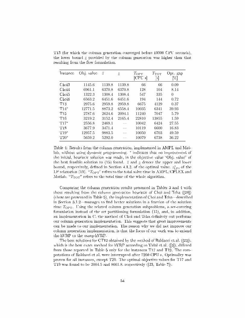
T13 (for which the column generation converged before 10000 CPU seconds),the lower bound z provided by the column generation was higher than thatresulting from the �ow formulation.
Instance Obj. value z z TOPT TTOT Opt. gap[CPU s] [s] [%]
Choi3 1145.6 1139.8 1139.8 66 66 0.09Choi4 6961.1 6370.8 6370.8 128 104 8.14Choi5 1322.3 1308.4 1308.4 547 335 0Choi6 6563.2 6451.6 6451.6 194 144 0.72T13 2975.6 2959.8 2959.8 6675 4129 0.37T14∗ 12771.5 8873.2 6558.4 10035 6341 39.93T15 2787.6 2624.6 2094.1 11240 7047 5.79T16 3219.2 3152.4 2165.4 22810 13855 1.59T17∗ 2556.8 2469.1 � 10042 6424 27.55T18 3677.9 3471.4 � 10119 6600 16.83T19∗ 12957.5 9883.5 � 10050 6703 49.59T20∗ 5659.2 5292.0 � 10079 6738 36.22
Table 4: Results from the column generation, implemented in AMPL and Mat-lab, without using dynamic programming. ∗ indicates that no improvement ofthe initial, heuristic solution was made, in the objective value �Obj. value� ofthe best feasible solution to (15) found. z and z denote the upper and lowerbound, respectively, de�ned in Section 4.1.2, of the optimal value, z∗LP, of theLP relaxation (19). �TOPT� refers to the total solve time in AMPL/CPLEX andMatlab. �TTOT� refers to the total time of the whole algorithm.
Comparing the column generation results presented in Tables 3 and 4 withthose resulting from the column generation heuristic of Choi and Tcha ([24])(these are presented in Table 5), the implementation of Choi and Tcha�describedin Section 3.1.2�manages to �nd better solutions in a fraction of the solutiontime TOPT. Using the relaxed column generation subproblems, a set-coveringformulation instead of the set-partitioning formulation (15), and, in addition,an implementation in C, the method of Choi and Tcha de�nitely out-performsour column generation implementation. This suggests that great improvementscan be made to our implementation. The reason why we did not improve ourcolumn generation implementation, is that the focus of our work was to extendthe hVRP to the many-hVRP.
The best solutions for CT12 obtained by the method of Baldacci et al. ([23]),which is the best exact method for hVRP according to Vidal et al. ([3]), di�eredfrom those reported in Table 5 only for the instances T17 and T19. The com-putations of Baldacci et al. were interrupted after 7200 CPU s. Optimality wasproven for all instances, except T20. The optimal objective values for T17 andT19 was found to be 2004.5 and 8661.8, respectively ([23, Table 7]).
54
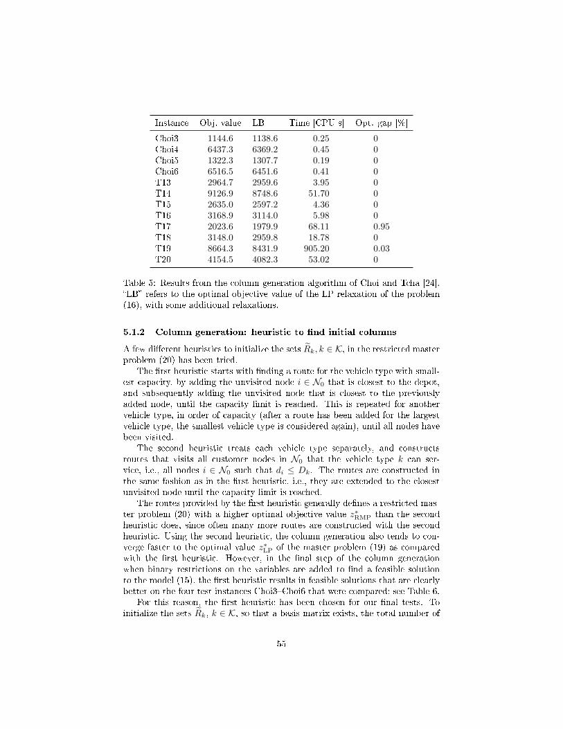
Instance Obj. value LB Time [CPU s] Opt. gap [%]
Choi3 1144.6 1138.6 0.25 0Choi4 6437.3 6369.2 0.45 0Choi5 1322.3 1307.7 0.19 0Choi6 6516.5 6451.6 0.41 0T13 2964.7 2959.6 3.95 0T14 9126.9 8748.6 51.70 0T15 2635.0 2597.2 4.36 0T16 3168.9 3114.0 5.98 0T17 2023.6 1979.9 68.11 0.95T18 3148.0 2959.8 18.78 0T19 8664.3 8431.9 905.20 0.03T20 4154.5 4082.3 53.02 0
Table 5: Results from the column generation algorithm of Choi and Tcha [24].�LB� refers to the optimal objective value of the LP relaxation of the problem(16), with some additional relaxations.
5.1.2 Column generation: heuristic to �nd initial columns
A few di�erent heuristics to initialize the sets Rk, k ∈ K, in the restricted masterproblem (20) has been tried.
The �rst heuristic starts with �nding a route for the vehicle type with small-est capacity, by adding the unvisited node i ∈ N0 that is closest to the depot,and subsequently adding the unvisited node that is closest to the previouslyadded node, until the capacity limit is reached. This is repeated for anothervehicle type, in order of capacity (after a route has been added for the largestvehicle type, the smallest vehicle type is considered again), until all nodes havebeen visited.
The second heuristic treats each vehicle type separately, and constructsroutes that visits all customer nodes in N0 that the vehicle type k can ser-vice, i.e., all nodes i ∈ N0 such that di ≤ Dk. The routes are constructed inthe same fashion as in the �rst heuristic, i.e., they are extended to the closestunvisited node until the capacity limit is reached.
The routes provided by the �rst heuristic generally de�nes a restricted mas-ter problem (20) with a higher optimal objective value z∗RMP than the secondheuristic does, since often many more routes are constructed with the secondheuristic. Using the second heuristic, the column generation also tends to con-verge faster to the optimal value z∗LP of the master problem (19) as comparedwith the �rst heuristic. However, in the �nal step of the column generationwhen binary restrictions on the variables are added to �nd a feasible solutionto the model (15), the �rst heuristic results in feasible solutions that are clearlybetter on the four test instances Choi3�Choi6 that were compared; see Table 6.
For this reason, the �rst heuristic has been chosen for our �nal tests. Toinitialize the sets Rk, k ∈ K, so that a basis matrix exists, the total number of
55

columns in the initial restricted master problem (20) should be greater than or
equal to the number of constraints, i.e.,∑k∈K |Rk| ≥ |N0| (see Appendix B.1).
This has been achieved by adding, for each customer node, one route that visitsonly that customer, using the vehicle with the largest capacity. However, byadding these routes to the routes generated by the heuristic, the best feasiblesolution to the formulation (15) found in the last column generation iteration,appears to be of lower quality (compare the objective values obtained when thealgorithm is initiated using the �First heuristic� with those obtained using the�First heuristic, extra routes� in Table 6). For this reason extra routes havenot been added in our standard version of the column generation algorithm.Instead, the problem of determining a basis matrix (adding arti�cial columns)is left to AMPL.
Instance Objective value
First heuristic Second heuristic First heuristic, extra routes
Choi3 1150.9 1157.8 1155.2Choi4 6484.8 6512.9 6987.1Choi5 1322.3 1333.6 1323.2Choi6 6524.4 6537.6 6537.6
Table 6: Results from column generation started using two di�erent heuristics,on the four smallest test instances in CT12. �Objective value� refers to the ob-jective value of the best feasible solution to the formulation (15) found, i.e., thevalue obtained in the last column generation iteration when binary requirementsare added.
5.1.3 Column generation: algorithms applied to the subproblem
The subproblems have been implemented such that they can either be solvedusing the mathematical formulations (23) and (23a)�(23e), (23h)�(23i), (24) inSection 4.1.1 (implemented in AMPL and CPLEX), or by using the dynamicprogramming algorithm described in Section 4.1.1 (implemented in Matlab).
Preliminary tests on the smallest test instances, i.e., Choi3�Choi6, solvingall subproblems to optimality, indicated that none of the two mathematical for-mulations (23) and (23a)�(23e), (23h)�(23i), (24) is signi�cantly better than theother; each formulation outperforms the other on some test instance. However,the latter formulation with the constraints (23c) removed (which is a valid for-mualtion) does not perform well on the small test instances; after only a fewcolumn generation iterations for the instance Choi3, the computations were ter-minated by AMPL with termination code 9, which is �an error code from theoperating system level which has generally been associated with out-of-memoryerrors� ([39]). Contrast this to the formulation (23), for which the column gen-eration algorithm for the instance Choi3 converges after 110 CPU seconds, andthe formulation (23a)�(23e), (23h)�(23i), (24), for which the column generationalgorithm for the instance Choi3 converges after 75 CPU seconds.
56
In our standard implementation, subproblems are �rst solved using the dy-namic programming algorithm, which is terminated after a time limit is exceededor after a certain number of partial paths in PNPP has been processed (it hasbeen set so that the limit on the number of paths is not restrictive). The timelimit is increased if, in a certain iteration, no routes with negative reduced costare found for any of the subproblems. When the time limit has been increased aprede�ned number of times and no more routes with negative reduced cost arefound, the subproblem is solved by AMPL and CPLEX, using the formulation(23a)�(23e), (23h)�(23i), (24). Here, each subproblem is also terminated eitherwhen a time limit is reached or when a certain number of routes with negativereduced cost have been found. This time limit can also be increased when nomore routes with negative reduced cost are found for any subproblem. In a �nalstep�if the column generation has not converged in the previous steps�all sub-problems are solved to optimality. Subproblems that are solved by AMPL andCPLEX use the CPLEX-option uppercutoff=0�meaning that nodes in thebranch-and-bound tree with an optimal value higher than zero are fathomed([40, p. 71])�since only routes with negative reduced costs are interesting.
Many con�gurations for solving the subproblems are possible. The con-�gurations for the time limit used in the standard implementation are shownin Table 7. The great di�erence in size between the test instances makes itnecessary to use di�erent time limit con�gurations for di�erent instances. Con-�gurations CONF1 and CONF4 are used for the small instances Choi3�Choi6,con�gurations CONF2 and CONF5 are used for the medium-sized instancesT13, T15�T16, and CONF3 and CONF6 are used for instances T14, T17�T20in the standard implementation. Since T14 is much more computationally de-manding than the other medium sized instances T13, T15�T16 (see the resultsin Section 5.1.1) it is therefore included in the latter group.
In addition to the time limit, a kind of tabu-strategy of partial columngeneration�described in Section 4.1.1�has also been implemented for the sub-problems. When the tabu-strategy is used, subproblems that do not yield anyroute with negative reduced cost for a pre-determined number of consecutivecolumn generation iterations, are not considered for a pre-determined numberof iterations. This strategy reduces the number of subproblems that need tobe solved each iteration. It is often the case that a subproblem that has notprovided a route with negative reduced cost for a number of iterations will notprovide one for many more iterations, so the negative impact of this procedureon the number of iterations needed for the column generation to converge shouldnot be great. In the standard implementation, a subproblem is not consideredagain for seven or four consecutive iterations (the number depending on thecurrent phase of the column generation solutiouree), if that subproblem has notprovided a route with negative reduced cost for two consequtive iterations (whendynamic programming is used) or for four consecutive iterations (when AMPLand CPLEX are used). Note that when a time limit is set for the subproblems,there may exist a route with negative reduced cost for a speci�c subproblem,even if no route is found during the solution course for that subproblem.
57

Con�g Dynamic programming AMPL
TSTART [CPU s] SMULT SNUMINC T1 [CPU s] T2 [CPU s]
CONF1 2 2 1 15 500CONF2 5 3 1 50 500CONF3 5 5 3 250 500CONF4 - - - 2 10CONF5 - - - 5 30CONF6 - - - 25 300
Table 7: Di�erent con�gurations of the time limit for the subproblems. TSTART
denotes the time limit for the dynamic programming in the �rst part of the col-umn generation algorithm. If no route with negative reduced cost is found forany of the subproblems in a speci�c column generation iteration, and optimalityhas not been veri�ed, then the time limit is multiplied by SMULT. This is doneSNUMINC times, after which the subproblem is solved by AMPL and CPLEX.The �rst time limit in AMPL and CPLEX is T1. If no route with negativereduced cost is found for any of the subproblems in a speci�c iteration, and op-timality has not been veri�ed, then the time limit is increased to T2. If no routewith negative reduced cost is found and optimality is still not been veri�ed, thenall subproblems are solved to optimality until the column generation algorithmhas converged. No values given for TSTART, SMULT, and SNUMINC means thatdynamic programming is not used. The computations can be interrupted aftera pre-de�ned time limit for the complete column generation algorithm has beenexceeded, for any of the con�gurations.
The gain from the CPLEX option uppercutoff=0 is in itself quite substan-tial, and together with the time limit and tabu-strategy for the subproblems,these extensions of the column generation algorithm led to greatly reduced solu-tion times. So for example did the solution time for test instance T13 decreasefrom 2.3 · 106 to 7.3 · 103 CPU seconds, when uppercutoff=0, time limit, andthe tabu-strategy were used instead of solving all subproblems to optimality inAMPL and CPLEX.
The improvements in solution time when using uppercutoff=0 and timelimits are illustrated for the instance T13 in Figures 4 and 5. The tabu-strategyfor subproblems was not used here, to illustrate why it is useful (it is often thecase that when a subproblem has not provided a route with negative reducedcost for a few iterations, it often will not do so for many more iterations, as canbe seen in both Figures 4 and 5).
In Figures 4 and 5, solution times for column generation subproblems forall vehicles A�F in the instance T13 are shown; for each speci�c vehicle, thesubproblems for which no route with negative reduced cost were found are in-dicated by circles. Figure 4 shows the subproblem solution times when all thesubproblems are solved to optimality in AMPL�for the larger vehicles the sub-problem solution times are very long (up to 50, 000 CPU s) in the second half
58

of the column generation algorithm. This amount of time is more time thanwhat is used by the whole column generation algorithm when using dynamicprogramming with time limits and uppercutoff=0, as shown in Figure 5.
0 10 20 30 40 500
10
20
30
40
50Time spent on the column generation subproblem, smallest vehicles
CP
U s
iteration
ABC
0 10 20 30 40 500
0.5
1
1.5
2x 10
5 Time spent on the column generation subproblem, largest vehicles
CP
U s
iteration
DEF
Figure 4: Time spent on solving the column generation subproblems for eachof the vehicles A�F in the instance T13. In each iteration the subproblems aresolved to optimality in AMPL. The vehicles D�F�having larger capacities�give rise to longer computing times than the vehicles A�C�with a smallercapacities. A circle indicates that the optimal value (the minimum reducedcost) of the corresponding subproblem is non-negative.
A few more iterations are needed when the subproblems are not solved tooptimality in each iteration in this way (see Figure 5) but the gain in total solu-tion time is great. After 58 column generation iterations, dynamic programmingwith the given time limit can no longer �nd any route with negative reducedcost for any of the vehicles. The subproblems are then solved to optimality inAMPL. This takes a lot more time than the time limit that was set for thedynamic programming, but nothing is actually gained in terms of the optimalobjective value of the restricted master problem. Even though AMPL managesto �nd a route with negative reduced cost in each of the iterations 59 and 60,no improvement is made in the objective value of the restricted master problemafter adding those routes. However, adding these routes makes it possible to
59

verify that the solution to the restricted master problem in iteration 58 (the lastiteration employing dynamic programming) is optimal in the complete masterproblem.
0 10 20 30 40 50 600
5
10
15Time spent on the column generation subproblem (Dynamic programming)
CP
U s
iteration
ABCDEF
58 58.5 59 59.5 60 60.5 610
10
20
30
40
50Time spent on the column generation subproblem (AMPL)
CP
U s
iteration
ABCF
58 58.5 59 59.5 60 60.5 610
1000
2000
3000
4000
5000Time spent on the column generation subproblem (AMPL)
CP
U s
iteration
DE
Figure 5: Time spent on the column generation subproblems for each vehicleA�F in the instance T13. Subproblems are solved by dynamic programmingin Matlab with a time limit the �rst 58 iterations, whereas in iterations 59�61subproblems are solved to optimality using CPLEX. The rings indicate that theminimum objective value (the minimum reduced cost) found for a subproblemis non-negative.
The impact of using uppercutoff=0 is demonstrated by the fact that thesolution time of the the subproblem for the largest vehicle (F) actually is lessthan that of C, D, and E (Figure 5). Compare with Figure 4, in which thesolution time of the subproblem for vehicle F is much greater than for the othervehicles. AMPL sends previously found solutions to CPLEX as a warm-startwhen solving the next subproblem [40, pp. 60�61]. Since only the parametersckij , (i, j) ∈ A, and Dk di�er between the subproblems ((23a)�(23e), (23h)�(23i),
60
(24)), when using uppercutoff=0 it is probably the case that the solution to thepreviously solved subproblem for vehicle E is utilized to start the subproblemsolution for vehicle F. Hence AMPL can quickly conclude that the optimal valueis greater than zero, without having to �nd this value.
5.2 The extended test instances, CT12EXT
To test the performance of the proposed algorithms in Section 4 formany-hVRP,the extended test instances, CT12EXT, were used. In CT12EXT, the vehiclesets are extended to include vehicles with all (integer) capacities between thelowest and highest capacity of the original instances; see Section 3.1.3. Theresulting instances thus contain between 91 and 381 di�erent vehicle types.
In Section 5.2.1, the straightforward model (15) of many-hVRP is assessed.The column generation applied to CT12 in Section 5.1.1 is here tested on theextended test instances of CT12EXT and the results are compared.
The extended instances CT12EXT have also been used to test the algo-rithms proposed for the restricted model (25). This model, when the vehicletype limit C is not restrictive, is equivalent to the straightforward model inthat share optimal solutions and thus also optimal values�although di�erentsolution methods are applied to the two models. Benders' algorithm applied tothe restricted model, with a non-restrictive vehicle type limit C, is assessed inSection 5.2.2, in which the results are also compared with the results obtainedfor the straightforward model presented in Section 5.2.1. A modi�ed Benders'algorithm, using projection of routes, which yielded great improvements in theperformance of the algorithm, is presented in Section 5.2.3. The convergence ofBenders' algorithm is discussed in Section 5.2.4, and Benders' algorithm with arestrictive limit C is evaluated in Section 5.2.5.
Results of tests of the straightforward restricted models using load dependentcosts are presented in Section 5.2.6.
The notation in Sections 5.2.2�5.2.4 follows that in Section 4.2.
5.2.1 Straightforward model with column generation
When the column generation algorithm for the straightforward model (15) wastested on the extended test instances CT12EXT, it was found that subproblemsfor vehicles with similar capacities often provide the same routes in the currentcolumn generation iteration�although with di�erent objective values/reducedcosts, because of the slightly di�erent cost structures. For the instances CT12,having more dissimilar vehicle cost structures, the subproblems mostly providedi�erent routes. The column generation algorithm was therefore adjusted sothat routes were added only from the subproblem that provided the lowestobjective value/reduced cost for the same route. Subproblems that did notprovide any route�either because no route with a negative reduced cost wasfound, or because the route found with a negative reduced cost was also foundin another subproblem, and with a lower reduced cost�for a pre-determinednumber of consecutive column generation iterations were as before not solved
61
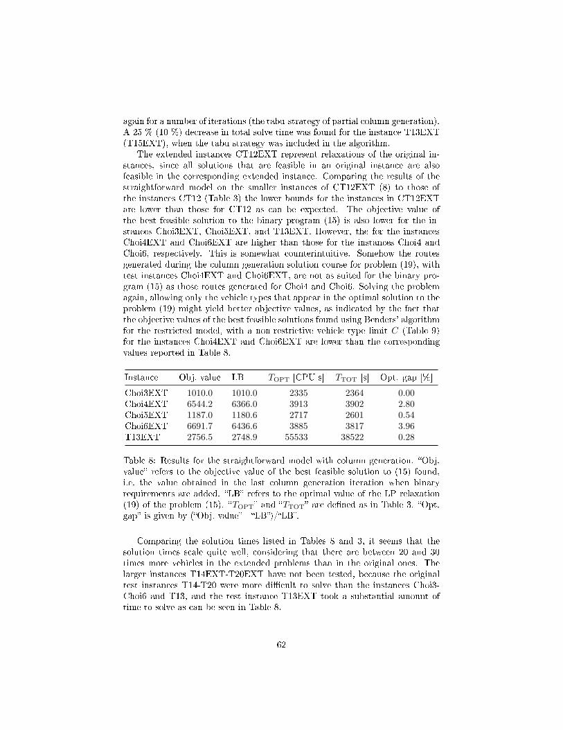
again for a number of iterations (the tabu-strategy of partial column generation).A 25 % (10 %) decrease in total solve time was found for the instance T13EXT(T15EXT), when the tabu strategy was included in the algorithm.
The extended instances CT12EXT represent relaxations of the original in-stances, since all solutions that are feasible in an original instance are alsofeasible in the corresponding extended instance. Comparing the results of thestraightforward model on the smaller instances of CT12EXT (8) to those ofthe instances CT12 (Table 3) the lower bounds for the instances in CT12EXTare lower than those for CT12 as can be expected. The objective value ofthe best feasible solution to the binary program (15) is also lower for the in-stances Choi3EXT, Choi5EXT, and T13EXT. However, the for the instancesChoi4EXT and Choi6EXT are higher than those for the instances Choi4 andChoi6, respectively. This is somewhat counterintuitive. Somehow the routesgenerated during the column generation solution course for problem (19), withtest instances Choi4EXT and Choi6EXT, are not as suited for the binary pro-gram (15) as those routes generated for Choi4 and Choi6. Solving the problemagain, allowing only the vehicle types that appear in the optimal solution to theproblem (19) might yield better objective values, as indicated by the fact thatthe objective values of the best feasible solutions found using Benders' algorithmfor the restricted model, with a non-restrictive vehicle type limit C (Table 9)for the instances Choi4EXT and Choi6EXT are lower than the correspondingvalues reported in Table 8.
Instance Obj. value LB TOPT [CPU s] TTOT [s] Opt. gap [%]
Choi3EXT 1010.0 1010.0 2335 2364 0.00Choi4EXT 6544.2 6366.0 3913 3902 2.80Choi5EXT 1187.0 1180.6 2717 2601 0.54Choi6EXT 6691.7 6436.6 3885 3817 3.96T13EXT 2756.5 2748.9 55533 38522 0.28
Table 8: Results for the straightforward model with column generation. �Obj.value� refers to the objective value of the best feasible solution to (15) found,i.e. the value obtained in the last column generation iteration when binaryrequirements are added. �LB� refers to the optimal value of the LP relaxation(19) of the problem (15). �TOPT� and �TTOT� are de�ned as in Table 3. �Opt.gap� is given by (�Obj. value� - �LB�)/�LB�.
Comparing the solution times listed in Tables 8 and 3, it seems that thesolution times scale quite well, considering that there are between 20 and 30times more vehicles in the extended problems than in the original ones. Thelarger instances T14EXT-T20EXT have not been tested, because the originaltest instances T14-T20 were more di�cult to solve than the instances Choi3-Choi6 and T13, and the test instance T13EXT took a substantial amount oftime to solve as can be seen in Table 8.
62

5.2.2 The restricted model with Benders' algorithm�non-restrictive
vehicle type limit C
Knowing an optimal solution to the LP relaxation (19) of the straightforwardmodel, for an instance in CT12EXT, the vehicle type limit C in the restrictedmodel can be set higher than the number of vehicle types used in the knownoptimal solution. This makes the optimal solution to the relaxation (26) of thestraightforward model, an optimal solution to (19). This enables a comparisonof the di�erent solutions strategies for the straightforward model (column gener-ation of Algorithm 1 and the restricted model (Benders' algorithm of Algorithm3). As described in Section 4.2, when Benders' algorithm is implemented forthe restricted model, Benders subproblems equal (19), but with a smaller setof vehicle types (including at most C types). Also, in each Benders iteration afeasible solution to the restricted model (26) is given�in contrast to the columngeneration applied to the straightforward model and which guarantees a feasiblesolution only in the last column generation iteration (when binary requirementsare added in the restricted master problem).
The results for the restricted model with a non-restrictive limit C, for thesmallest instances of CT12EXT, are given in Table 9. These results are com-pared with those obtained by using column generation for the straightforwardmodel, listed in Table 8. Results for T13EXT are not included here, becausecalculating the values of the Benders dual variables γ is too time-consumingfor this instance; especially for γk for the larger vehicle types k. Only vehiclesamong the 32 smallest vehicle types are used in an optimal solution, so usingthe lower bound suggested in Appendix C.3 to reduce the set of vehicle typeswould probably result in big improvements�as would using the lower bound onγk suggested in Section 4.2.5.
Benders' algorithm performs better than the the column generation for thestraightforward model for some of the small instances, and quite a lot worsefor some. For the instances Choi4EXT and Choi6EXT, Benders' algorithmconverges to the optimal solution to (26) (being an optimal solution also to (19))in just two and three iterations, respectively, taking less computing time than thecolumn generation approach for the straightforward model. The best objectivevalues of (25) found for these instances, when applying Benders' algorithm to therestricted model, are also better than those found applying column generationto the straightforward model. On the contrary, for the instances Choi3EXTand Choi5EXT, Benders' algorithm does not pick the vehicles that are usedin the optimal solution to (26) even after 100 Benders iterations, even thoughthis takes a lot more time than solving the straightforward model; see Table8. The biggest di�erence between the original and extended sets of instances isthat for Choi4EXT and Choi6EXT, the cost structure is such that only vehicletypes among the �ve smallest are used in the optimal solutions to (26); thismight explain why Benders' algorithm converges before 100 Benders iterationsfor these instances but not for Choi3EXT and Choi5EXT.
63

Instance C Obj1 Obj2 LB TOPT TTOT It Opt. gap[CPU s] [s] [%]
Choi3EXT 10 1010.5 1010.5 893.3 10124 31573 100 0.05Choi4EXT 4 6366.0 6484.7 6366.0 1101 1119 3 1.86Choi5EXT 13 1181.4 1188.7 1067.6 59302 52205 100 0.69Choi6EXT 6 6436.6 6580.8 6436.6 1304 1298 4 2.24
Table 9: Results for Benders' algorithm. �C� is the parameter value of the ve-hicle type limit that restricts the number of vehicle types used in any solutionto the problems (26) and (25). It is set to two units larger than the number ofvehicle types used in the optimal solution to (19), which is thus not restrictive.�Obj1� refers to the objective value of the best optimal solution to Benders sub-problem, which is an upper bound on the optimal objective value of (26). �Obj2�refers to the objective value of the best solution found when adding binary re-strictions in the last iteration of the column generation algorithm performed tosolve the Benders subproblem in each Benders iteration; it is an upper boundon the optimal objective value of (25). �LB� refers to the optimal objectivevalue of Benders restricted master problem in the last Benders iteration, whichis a lower bound on the optimal objective value of (26), and therefore also alower bound on the optimal objective value of (25). �TOPT� and �TTOT� arede�ned as in Table 3. �It� refers to the number of Benders iterations performed.Maximally 100 Benders iterations have been performed. �Opt. gap� is given by(�Obj. value� - v∗)/v∗, where v∗ is the optimal value of (26). Since the limit Cis not restrictive, v∗ equals the lower bound presented in Table 8.
Next, more detailed results are provided for the instance Choi3EXT. Theoptimal objective values of Benders subproblem and Benders restricted masterproblem with vehicle type limit C = 10, i.e., the restricted model with at mostten di�erent vehicle types used in any solution, are shown for each Bendersiteration in Figures 6 and 7. The best objective value of Benders subproblemfound, 1010.5, is not found until iteration 81. It is close to the optimal value,1010.0; see Table 8. The optimal objective value of Benders restricted masterproblem increases in each iteration, but after 20 iterations the increase is verysmall, although it is still far from the optimal objective value of Benders masterproblem.
Even though the optimal solution to (26) is not found during the 100 iter-ations for Choi3EXT, the vehicle types that are used in the optimal solution13
are chosen quite frequently, which is illustrated in Figure 8. A similar patternwas found for the other instances tested as well. Figure 8 also shows that of the101 vehicle types, only vehicles among the 39 smallest types are chosen in anyBenders iteration.
13The optimal solution to the relaxed problem (26) is integer for Choi3EXT, and is thereforealso an optimal solution to (25). This is, however, not a general property.
64

0 10 20 30 40 50 60 70 80 90 1001000
1020
1040
1060
1080
1100
1120
1140
obje
ctiv
e va
lue
Optimal objective values of Benders subproblems
Benders iteration
Optimal value of Benders subproblemOptimal value of Benders master problem
Figure 6: Optimal objective values of Benders subproblems over 100 iterations,for Choi3EXT with vehicle type limit C = 10; the best value, 1010.5, is attainedat iteration 81. The optimal objective value of Benders master problem is 1010.
0 10 20 30 40 50 60 70 80 90 100−7000
−6000
−5000
−4000
−3000
−2000
−1000
0
1000
Optimal objective values of Benders restricted master problems
obje
ctiv
e va
lue
Benders iteration
Optimal value of Benders restricted master problemOptimal value of Benders master problem
Figure 7: Optimal objective values of Benders restricted master problems over100 iterations, for Choi3EXT with vehicle type limit C = 10. The mean increasein objective value between two successive Benders iterations is 4.1 (0.3) foriterations 10�50 (50�100); the best value attained is 893 (at iteration 100) ascompared to the optimal value, 1010.0, of Benders master problem.
65

0 5 10 15 20 25 30 35 390
10
20
30
40
50
60
70
80
90
100
perc
enta
ge o
f ite
ratio
ns
vehicle type
Percentage of 100 iterations in which each vehicle type is chosen
Figure 8: The percentage of 100 Benders iterations in which each of the vehicles(of type/size 1�101) is chosen, for Choi3EXT with vehicle type limit C = 10.The known optimal solution uses the vehicle set {1, 2, 10, 17, 18, 22, 23, 25},which is marked by lighter bars.
An interesting fact is that after a few Benders iterations, the di�erence be-tween the objective values of the �rst and last iterations (before adding binaryrestrictions on the variables) of the column generation applied to Benders sub-problem is often very small when the column generation is warm-started withroutes from solutions xl to previous Benders iterations; see Section 4.2.4. Theusefulness of re-using routes in this way is demonstrated in Figure 9 for theinstance Choi3EXT with vehicle type limit C = 10. In only thirteen of the 100Benders iterations was the di�erence non-zero, and the greatest di�erence wasfound during the �rst iterations. It is also in those �rst Benders iterations thatthe objective value of Benders restricted master problem increases the most, seeFigure 7.
This e�ect is also apparent in the computation time required for the columngeneration of Benders subproblems, as shown in Figure 10. The column gener-ation for Benders subproblem in the �rst two Benders iterations requires morethan twice the time that is required for the following iterations; this is consistentwith the pattern apparent in Figure 9, in which the column generation in thethree �rst Benders iterations results in a much larger di�erence than do the lateriterations. The time spent on calculating the dual variable value γL from thedual variable value πL�found in the last iteration of the column generation�isless than the time spent on the column generation in all the Benders iterations.It takes less than one second to solve Benders restricted master problem, whichis only a fraction of the time spent on Benders subproblems, hence the timespent on solving Benders restricted master problem is not included in Figure10.
66
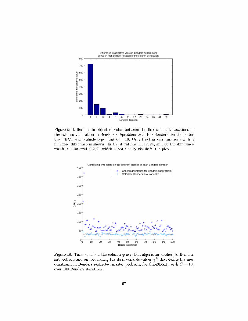
1 2 3 4 5 6 11 17 20 24 36 44 590
100
200
300
400
500
600
700
800
diffe
renc
e in
obj
ectiv
e va
lue
Benders iteration
Difference in objective value in Benders subproblembetween first and last iteration of the column generation
Figure 9: Di�erence in objective value between the �rst and last iterations ofthe column generation in Benders subproblem over 100 Benders iterations, forChoi3EXT with vehicle type limit C = 10. Only the thirteen iterations with anon-zero di�erence is shown. In the iterations 11, 17, 24, and 36 the di�erencewas in the interval [0.2, 2], which is not clearly visible in the plot.
0 10 20 30 40 50 60 70 80 90 1000
50
100
150
200
250
300
350
400
CP
U s
Computing time spent on the different phases of each Benders iteration
Benders iteration
Column generation for Benders subproblemCalculate Benders dual variables
Figure 10: Time spent on the column generation algorithm applied to Benderssubproblem and on calculating the dual variable values γL that de�ne the newconstraint in Benders restricted master problem, for Choi3EXT, with C = 10,over 100 Benders iterations.
67

5.2.3 Improved Benders' algorithm using projection of routes
Studying the optimal routes that are part of the solutions xl to (BendersSP(yl)),for Benders iterations l = 1, . . . , L, i.e., studying the sets Rl, de�ned in Section4.2.4, it becomes clear that in some iterations the routes used in the optimalsolution to (BendersSP(yl)) actually form an optimal solution to (26), however,they are not paired with the correct vehicle types.
In Section 4.2 we describe the procedure �projection of routes�, in whichroutes being solutions to Benders subproblems in earlier iterations are com-bined with other vehicle types (that were not allowed in those subproblems butwhich provide lower objective values). This procedure has been implementedin order to improve the performance of Benders' algorithm. If such vehicletypes are found and de�ne a feasible Benders subproblem, then they are used inthe next Benders iteration. This procedure seems to yield great improvementsto Benders' algorithm for the instances Choi3EXT and Choi5EXT (for whichBenders' algorithm was found too perform poorly in Section 5.2.2).
0 5 10 15 20 251000
1020
1040
1060
1080
1100
1120
1140
obje
ctiv
e va
lue
Optimal objective values of Benders subproblems
Benders iteration
Optimal value of Benders subproblemOptimal value of Benders master problem
Figure 11: Optimal objective values of Benders subproblems over 24 iterationswhen the projection of routes is used, for Choi3EXT with the vehicle type limitC = 10. The best objective value 1010.0, which equals the optimal value ofBenders master problem, was found in iteration 15 by projecting routes fromiteration 14.
These improvements are illustrated in Figure 11 for the instance Choi3EXT,with the vehicle type limit C = 10. Projection of routes is tried out in everyiteration from iteration 4; it is successful in iterations 5, 6, and 15. We comparethis with the results shown in Figure 6 (Section 5.2.2), for the same instancesolved without the projection of routes procedure. Without the projection of
68

routes, the best objective value (1010.5) of Benders subproblem over 100 Ben-ders iterations is found at iteration 81. When using projection of routes, thissolution is found already at iteration six. Also, the best objective value (1010.0),found at iteration 15 when using the projection of routes, is optimal in (26).
Similar results were obtained for Choi5EXT, when projection of routes wasused. The optimal objective value of (26) for Choi5EXT, 1180.6, was found inBenders subproblem in Benders iteration 16, while the best objective value ofBenders subproblem over 100 iterations withouth using the projection of routeswas 1181.4.
5.2.4 Convergence of Benders' algorithm
Unfortunately, as discussed in Section 4.2.3, Benders' algorithm does not alwaysterminate when the optimal solution to (26) has been found, if not all necessaryconstraints to Benders master problem have been generated. This happensfor the instance Choi3EXT with the vehicle type limit C = 10 (which is notrestrictive), both when the projection of routes is used and when it is not (seeSections 5.2.2 and 5.2.3). Using the projection of routes, the optimal value ofBenders master problem is found at Benders iteration 15, but the optimalityis not veri�ed until iteration 2342 (in order to speed up the convergence onlythe 30 smallest vehicle types of Choi3EXT were considered). A similar lateveri�cation of the optimality was observed for the instance Choi5EXT.
The optimality for Choi3EXT, with C = 10, could actually have been ver-i�ed in iteration 16 if other values of Benders dual variables γ15 would havebeen found in Benders iteration 15. The values π15 found in Benders iteration15 yields that γ15 ≤ 0 and γ15 6= 0 (here, π15 is the dual variable value to theproblem (30) found in the last iteration of the column generation for Benderssubproblem at Benders iteration 15, and γ15 is calculated according to Claim2). The optimality criterion (32) of Benders' algorithm is not satis�ed in Ben-ders iteration 15. However, if the column generation for Benders subproblem iscontinued a couple of iterations, allowing for all vehicle types in K, no improve-ment is made to the objective value of the column generation restricted masterproblem, and optimality of x15 in the model (19) is veri�ed by the optimalitycriterion for column generation (implying that (x15, y15) is optimal in (26)).A new dual solution π to the column generation restricted master problem isfound, for which γ = 0 (where γ is calculated using π according to Claim 2).It holds that π is feasible and optimal in the dual of Benders subproblem inBenders iteration 15. If (π, γ) were used to de�ne the new constraint to Ben-ders restricted master problem in Benders iteration 15, instead of (π15,γ15),optimality of (x15, y15) in (26) could have been veri�ed in Benders iteration 16using the criterion (34), since then the inequality v16 ≥
∑i∈N0
π0i holds, and
we have that the inequalities v16 ≤ v∗ and∑i∈N0
π0i ≥ v∗ hold. This is a
general result, i.e., if the values of the Benders dual variables γ equal zero insome Benders iteration, then optimality would be veri�ed in the next Bendersiteration if the criterion (34) was used.
Assume that the vehicle type limit C is not restrictive. According to (31),
69
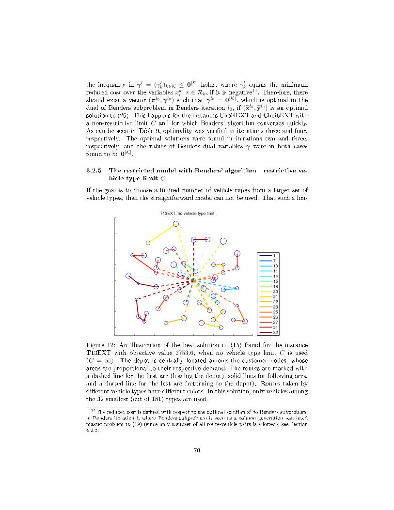
the inequality in γl = (γlk)k∈K ≤ 0|K| holds, where γlk equals the minimumreduced cost over the variables xkr , r ∈ Rk, if it is negative14. Therefore, thereshould exist a vector (πl0 ,γl0) such that γl0 = 0|K|, which is optimal in thedual of Benders subproblem in Benders iteration l0, if (xl0 , yl0) is an optimalsolution to (26). This happens for the instances Choi4EXT and Choi6EXT witha non-restrictive limit C and for which Benders' algorithm converges quickly.As can be seen in Table 9, optimality was veri�ed in iterations three and four,respectively. The optimal solutions were found in iterations two and three,respectively, and the values of Benders dual variables γ were in both casesfound to be 0|K|.
5.2.5 The restricted model with Benders' algorithm�restrictive ve-
hicle type limit C
If the goal is to choose a limited number of vehicle types from a larger set ofvehicle types, then the straightforward model can not be used. That such a lim-
T13EXT, no vehicle type limit
1
7
10
11
14
15
18
20
21
22
23
25
26
27
31
32
Figure 12: An illustration of the best solution to (15) found for the instanceT13EXT with objective value 2753.6, when no vehicle type limit C is used(C = ∞). The depot is centrally located among the customer nodes, whoseareas are proportional to their respective demand. The routes are marked witha dashed line for the �rst arc (leaving the depot), solid lines for following arcs,and a dotted line for the last arc (returning to the depot). Routes taken bydi�erent vehicle types have di�erent colors. In this solution, only vehicles amongthe 32 smallest (out of 181) types are used.
14The reduced cost is de�ned with respect to the optimal solution exl to Benders subproblemin Benders iteration l, where Benders subproblem is seen as a column generation restrictedmaster problem to (19) (since only a subset of all route-vehicle pairs is allowed); see Section4.2.2.
70

itation can be imposed constitutes a valuable feature of the restrictive model,which could result in a greater �exibility of the resulting �eet.
Figure 12 illustrates a feasible solution for the instance T13EXT in whichthe allowed number of vehicle types used is unlimited, and Figure 13 shows afeasible solution in which the number of vehicle types is limited to four. Thesolution illustrated in Figure 13 was obtained using Benders' algorithm, byrestricting the vehicle set to the 50 smallest vehicle types (only vehicles fromthe 32 smallest vehicle types were used in the optimal solution to T13EXT,when no vehicle type limit was set).
For the instance T13EXT with C = 4 (Figure 13), four vehicle types inthe range [22, 31] were used, whereas for the case with a non-restrictive vehicletype limit (Figure 12), 16 vehicle types in the range [1, 32] were used. Hence,for this instance, out of the totally 181 vehicle types only vehicles among the32 smallest types were used. Even though the objective value (2838.2) of thesolution for the case with C = 4 is greater than that (2753.6) for the case withnon-restrictive vehicle type limit, it is still lower than the optimal objective value(2964.7) of the original test instance T13 (see Section 5.2.1), which includes sixvehicle types.
T13EXT, vehicle type limit C=4
22
26
29
31
Figure 13: An illustration of the best solution to (25) found for the instanceT13EXT with objective value 2838.2, with vehicle type limit C = 4. In thissolution, only vehicle types in the range [22, 32] are used, out of 181 vehicletypes. Information about how to interpret the plot is found in Figure 12.
Choosing only a limited number of vehicle types, by using Benders' algorithmwith projection of routes for the restricted model (25), with a restrictive vehicletype limit C, seems to work quite well. The biggest disadvantage is that itmay take a long time to verify optimality using Benders' algorithm. When
71

terminating after a large number of Benders iterations it is often revealed thatthe best solution was found early in the solution course.
For the instance Choi3EXT with C = 6 a feasible solution with objectivevalue 1012.4 is found after eight Benders iterations when applying the projectionof routes, and this value is not improved during the following 142 Bendersiterations (since with C =∞ the optimal solution, with objective value 1010.0,contains eight di�erent vehicle types, the limit C = 6 is restrictive). Thissuggests that Benders' algorithm can be successfully used as a heuristic, thusterminated after a pre-speci�ed time limit or no improvement of the objectivevalue of Benders subproblem has been observed during a pre-speci�ed numberof iterations.
5.2.6 Load dependent costs
Both the straightforward model (15) and the restricted model (25) has beentested using load dependent costs, as described in Section 4.3. The parame-ters Qdist and Qload were set to 1.4 and 0.05, respectively, by testing di�erentcombinations for T13EXT using the straightforward model, and choosing thosevalues that resulted in reasonable solutions.
Load dependent cost Obj. value LB TOPT [CPU s] TTOT [s]
Yes 2775.6 2801.9 34113 27243No 2753.6 2748.9 35032 17658
Table 10: Results for the straightforward model using the column generationfor the instance T13EXT, with and without load dependent costs. �Obj. value�refers to the objective value of the best feasible solution to (15) found, i.e. thevalue obtained in the last column generation iteration when binary requirementsare added�given in the original cost of T13EXT. �LB� refers to the optimalvalue of the LP relaxation (19) of the problem (15). �TOPT� refers to the totalsolve time in AMPL/CPLEX and Matlab. �TTOT� refers to the total time ofthe whole algorithm.
Since some changes were made to the mathematical formulation of the col-umn generation subproblem to enable the inclusion of load dependent costs(compare formulations (23a)�(23e), (23h)�(23i), (24) and (37)), the results us-ing load dependent costs are compared to results obtained by setting Qdist = 1and Qload = 0, which is equivalent to not having load dependent costs. Thismakes the comparison of solution times more relevant. In Table 10, resultsfor the straightforward model using column generation, with and without loaddependent costs, are presented for the instance T13EXT. The load dependentobjective values have been converted to the original cost (by calculating the costof the solution using (15a)), for ease of comparison. The total solve time TOPT
when using load dependent costs is less than when load dependent costs are notused, while the opposite is true for the total time TTOT.
72
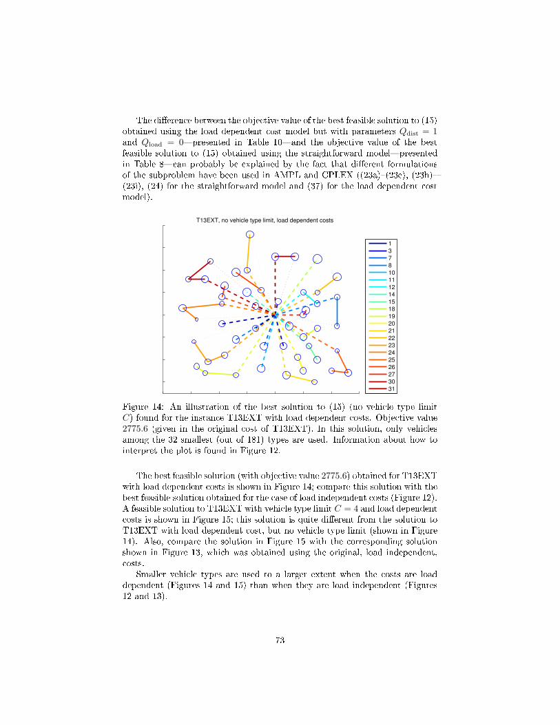
The di�erence between the objective value of the best feasible solution to (15)obtained using the load dependent cost model but with parameters Qdist = 1and Qload = 0�presented in Table 10�and the objective value of the bestfeasible solution to (15) obtained using the straightforward model�presentedin Table 8�can probably be explained by the fact that di�erent formulationsof the subproblem have been used in AMPL and CPLEX ((23a)�(23e), (23h)�(23i), (24) for the straightforward model and (37) for the load dependent costmodel).
T13EXT, no vehicle type limit, load dependent costs
1
3
7
8
10
11
12
14
15
18
19
20
21
22
23
24
25
26
27
30
31
Figure 14: An illustration of the best solution to (15) (no vehicle type limitC) found for the instance T13EXT with load dependent costs. Objective value2775.6 (given in the original cost of T13EXT). In this solution, only vehiclesamong the 32 smallest (out of 181) types are used. Information about how tointerpret the plot is found in Figure 12.
The best feasible solution (with objective value 2775.6) obtained for T13EXTwith load dependent costs is shown in Figure 14; compare this solution with thebest feasible solution obtained for the case of load independent costs (Figure 12).A feasible solution to T13EXT with vehicle type limit C = 4 and load dependentcosts is shown in Figure 15; this solution is quite di�erent from the solution toT13EXT with load dependent cost, but no vehicle type limit (shown in Figure14). Also, compare the solution in Figure 15 with the corresponding solutionshown in Figure 13, which was obtained using the original, load independent,costs.
Smaller vehicle types are used to a larger extent when the costs are loaddependent (Figures 14 and 15) than when they are load independent (Figures12 and 13).
73

T13EXT, vehicle type limit C=4, load dependent costs
12
22
28
31
Figure 15: An illustration of the best solution to (25) found for the instanceT13EXT with load dependent costs and with vehicle type limit C = 4, for testinstance T13EXT with load dependent costs. Objective value 2882.6 (given inthe original costs of T13EXT). In this solution, only vehicle types in the range[12, 31] are used, out of 181 vehicle types. Information about how to interpretthe plot is found in Figure 12.
74

6 Discussion
We have extended the standard heterogeneous vehicle routing problem (hVRP)to include a large set of vehicle types, then called many-hVRP. Further, we havedeveloped and tested models and algorithms for many-hVRP.
The results of the tests performed on the original test instances CT12 (seeSection 3.1.3) show that great improvements in the solution times were achieved�as demonstrated for the instance T13�using the time limit, the CPLEX-optionuppercutoff=0, and the tabu-strategy of partial column generation (see Section5.1.3). The tabu-strategy takes advantage of the fact that many subproblemsare similar for extended test instances CT12EXT. The time limit also a�ects thetabu-strategy, since subproblems which do not yield a route with negative re-duced cost within the given time limit for a few consecutive column generationiterations�so that those subproblems are skipped the following iterations�could have yielded routes with negative reduced cost given a more generoustime limit. For the larger test instances, this has a great positive e�ect on thesolution time of the column generation algorithm.
The results of the test performed on the extended test instances, CT12EXT,indicate that the straightforward model with column generation performs bet-ter than the restricted model with Benders' algorithm, when a non-restrictivevehicle type limit is set (which then has the same optimal solutions). Benders'algorithm converges very slowly for some test instances. With the implementedprojection of routes procedure, the performance of Benders' algorithm can beimproved�as demonstrated for the instance Choi3EXT�so that an optimal so-lution is found much sooner; however, the optimality of the solution still takesa very long time to verify.
Advantages of using Benders' algorithm are indicated by the following: aclear pattern emerges in which some vehicles types, which are part of an opti-mal set of vehicle types, are chosen more often than other vehicle types. Eachconstraint that is added to Benders restricted master problem has a nice inter-pretation as the objective value of the optimal solution to Benders subproblemplus a weighted sum of �reduced costs� (see Section 4.2.2), thus the collected in-formation gained from the �reduced costs� of previous solutions to Benders sub-problem is used when new vehicle types are chosen in each Benders iteration�this seems to provide a good guide for choosing new vehicle types. But, eventhough Benders' algorithm succeeds in choosing optimal vehicle types more of-ten than non-optimal vehicle types, the speci�c con�guration of the optimal setof vehicle types is sometimes hard to �nd. After a few iterations, the vehiclesthat are chosen do not seem to yield any improvements to previous solutions, inthe sense that there is no di�erence between the �rst and last iteration of thecolumn generation algorithm used to solve Benders subproblem (when the col-umn generation is warm-started with routes from optimal solutions to Benderssubproblems from previous iterations).
These properties of Benders' algorithm suggest that it may constitue a goodbasis for a heuristic, when the set of vehicle types is even larger than in thetest instances CT12EXT. Since an optimal con�guration of vehicle types can
75

often be found among the vehicle types that are frequently chosen by Benders'algorithm, and those vehicle types that are frequently chosen typically form amuch smaller set than the whole set of vehicle types, the set of vehicle types canafter a few Benders iterations be reduced to the types that have been frequentlychosen�resulting in a problem instance that is easier to solve.
The set of optimal routes for a given problem depends to a great extenton the vehicle types that are available. The improvements gained by usingthe projection of routes procedure suggest that Benders' algorithm succeeds inchoosing vehicle type con�gurations which yield Benders subproblems whoseoptimal solutions are composed by high quality routes. Using only those routesthat were part of previous optimal solutions to Benders subproblems, projectionof routes has been found to determine the optimal con�guration of vehiclesand routes. Thus, for problems instances where the set of vehicle types aremuch larger than those in the set of extended test instances CT12EXT, a goodapproach may be to temporarily restrict the set of vehicle types, and use someprocedure similar to the projection of routes�where vehicle types that are notpart of the restricted set are allowed to be matched with routes from solutionsto Benders subproblems�to �nd better solutions after a number of Bendersiterations have been performed, and extend the restricted set accordingly.
The restricted model, with a restrictive vehicle type limit C, was shown toyield solutions with di�erent characteristics than with an non-restrictive limit.Extending the straightforward and the restricted model, to include load depen-dent cost, also worked well; the solution times were not greatly impacted, andsolutions with slightly di�erent characteristics were found when load dependentcosts were considered�vehicle types with smaller capacities were used moreoften than when load independent costs were considered. Other extensions,mentioned in Section 3, can be similarly incorporated into the models.
6.1 Future research and development
To improve the performance of the proposed algorithms, several important ad-justments can be made. For the straightforward model, using column genera-tion, the dynamic programming algorithm should be implemented in C ratherthan in Matlab. Also, the column generation subproblems should be relaxed,as is done in many implementations of column generation for vehicle routingproblems (see Section 2.2) by Choi and Tcha [24], among others. The set-partitioning problem should be turned into a set-covering problem, solved using(possibly heuristic) branch-and-price. The lower bound, described in AppendixC.3, should be used to reduce the set of vehicle types. The results in Section5.1.1 suggest these changes would result in shorter computation times and thatsolutions with better objective values would be found.
For the restricted model, using Benders' algorithm, the relaxation suggestedfor the column generation subproblems should be applied to the problems (31)that are solved in each Benders iteration, as is suggested in Section 4.2.5. Thisis an important change, since in each Benders iteration, the model (31) needsto be solved for each vehicle type.
76

The models should also be changed to include more features of real life prob-lems. Even bigger sets of vehicles could be handled as suggested in Section 6.The load dependent costs could be made more realistic by letting the parametersQdist and Qload be arc-dependent; only minor adjustments to the code would benecessary to allow for this. Other extensions, such as time windows can easilybe incorporated into the models. With tight time-windows, the problem mayactually be easier to solve ([15]). An extended model could be based on thetechniques used by Ceselli et al. in [41], who consider a hVRP with multipledepots, as well as
time windows associated with depots and customers; incompatibilityconstraints between goods, depots, vehicles, and customers; max-imum route length and duration; upper limits on the number ofconsecutive driving hours and compulsory drivers' rest periods; thepossibility of skipping some customers and using express courier ser-vices instead of the given �eet to ful�ll some orders; the option ofsplitting up the orders; and the possibility of open routes that donot terminate at depots [41, abstract],
using a column generation algorithm with dynamic programming for the sub-problems. In Betinelli et al. ([15]), a similar hVRP with multiple depots andtime windows is solved, using a branch-and-cut-and-price heuristic. The au-thors state that it is probably the heterogeneous �eet that �really complicatesthe problem� [15, p. 735], but that their implementation often performs bet-ter than other heuristics from the literature. Heuristics such as these�basedon mathematical programming techniques�are becoming more popular, as wasmentioned in Section 3. The �ndings in [15] indicate that the models developedin this thesis could be competitive as heuristics for the many-hVRP.
We think that the solution methods developed in this thesis, in which thedi�cult problem of handling a large set of vehicle types is dealt with, form apromising foundation on which to build more complex models. As indicatedin the beginning of Section 3, there are many possible extensions of the stan-dard vehicle routing problem. To further develop the models and algorithmsdeveloped in this thesis in order to construct a framework that is relevant toreal-life problems, extensions of the many-hVRP models should be considered,more complex data sets should be used, and the solution algorithms should befurther developed according to the suggestions above.
77

Appendices
A Notation
A vector x ∈ Rn is understood to be a column-vector, and the scalar productof two vectors x,y ∈ Rn is written x>y. The two vectors x ∈ Rn1 ,y ∈ Rn2
are concatenated as z := (x,y), where z ∈ Rn1+n2 is assumed to be a columnvector. Furthermore, when given variables (xi)i∈I , where I denotes a set ofindices, the vector x ∈ R|I| is implicitly assumed to equal (xi)i∈I . If no orderis imposed on the index sets I and J , given a matrix A := (a>i )i∈I ∈ R|I|×|J |,where ai, i ∈ I are vectors in R|J | that de�ne the rows of A, and given a vectorx := (xj)j∈J , the matrix-vector product Ax is de�ned by the assumed ordering,so that for each i0 ∈ I, (Ax)i0 := a>i0x :=
∑j∈J (ai0)jxj . Similar notation
is used when variables are indexed using several sets of indices I1, . . . , In, as(xi1,...,in)i1∈I1,...,in∈In .
B Column generation
Here a thorough description of column generation is given. In Appendix B.1,a Dantzig-Wolfe decomposition of a linear program is presented together withthe mathematical theory that column generation of the decomposed problem isbased. In Appendix B.2 a Dantzig-Wolfe decomposition and column generationalgorithm for an integer program is presented. It is shown to provide a betterlower bound than the linear programming relaxation of the original problem(i.e., when the integrality requirements are relaxed).
B.1 Linear program
This presentation, unless otherwise indicated, is based on [9, Chapters 2.6, 3.3�3.4], and on linear programming theory from the textbook [4].
Here, column generation in connection with a Dantzig-Wolfe decompositionis presented in more detail, but the same theory can be applied to columngeneration as it is presented in Section 2.1. Using Dantzig-Wolfe decompositionhas the advantage that special structures in the problem can be utilized [8].Consider the linear program
(LP) minx
c>x, (38a)
s.t. Dx = d, (38b)
Ax = b, (38c)
x ≥ 0n, (38d)
where c, x ∈ Rn, d ∈ Rm1 , b ∈ Rm2 , D ∈ Rm1×n and A ∈ Rm2×n. The set offeasible solutions to (LP) is assumed to be non-empty and bounded.
78

When decomposing the problem, the constraints (38b) are regarded as com-plicating. This could be desirable if the problem has a speci�c structure, sothat the constraints (38b) and (38c) are easier to deal with separately, orif (38b) represents linking constraints [42]. Then, de�ning the polyhedronXLP := {x ≥ 0n | Ax = b}, any x ∈ XLP can be expressed as a convexcombination of its extreme points xp, p ∈ P, i.e., x :=
∑p∈P αpx
p such that∑p∈P αp = 1, αp ≥ 0, p ∈ P hold. The model (LP) can thus be rewritten as the
complete master problem
(DW) minα
∑p∈P
αpc>xp,
s.t.∑p∈P
αpDxp = d,
∑p∈P
αp = 1,
αp ≥ 0, p ∈ P.
(DW) is called the Dantzig-Wolfe formulation of (LP). Whereas (LP) has ncolumns, the decomposed problem (DW) contains one column for each extremepoint of the polyhedron XLP; hence, there are |P| columns in (DW). If |P| is avery large number, column generation can be a good approach to solving (DW).
De�ning a subset P ⊂ P, the column generation restricted master problem isgiven by
minα
∑p∈ eP
αpc>xp, (39a)
s.t.∑p∈ eP
αpDxp = d, (39b)
∑p∈ eP
αp = 1, (39c)
αp ≥ 0, p ∈ P. (39d)
The linear programming dual problem of the restricted master problem is givenby
maxπ,q
(d>π + q
), (40a)
s.t. (Dxp)>π + q ≤ c>xp, p ∈ P, (40b)
where π ∈ Rn, q ∈ R. The column generation subproblem is given by
z∗SubP := minp∈P
(c>xp − (Dxp)>π∗ − q∗
), (41)
where (π∗, q∗) is an optimal solution to (40). As is described in Section 2.1,in each column generation iteration the restricted master problem�in this case
79

(39)�is solved, after which the solution to the subproblem�in this case (41)�either yields a column/extreme point to be added to the restricted master prob-lem (i.e., if z∗SubP < 0) or establishes that an optimal solution to the completemaster problem has been found (i.e., if z∗SubP = 0). The problem (LP) hasbeen decomposed, so that constraints (38b) and (38c) are dealt with separately,with (38b) taken care of in the restricted master problem and (38c) in the sub-problem. In the remainder of this section, the theory behind this algorithm ispresented.
For ease of notation, let ωp := c>xp, dp := (Dxp, 1), and d := (d, 1), sothat (39a) can be written as minα
∑p∈P αpωp and (39b)�(39c) as∑
p∈Pαpdp = d.
As mentioned in Section 2.1, an optimal solution to the restricted master prob-lem (39) can be found in an extreme point to the feasible set of solutions de�nedby the constraints (39b)�(39d). It holds that any such extreme point can haveat most m1 + 1 non-zero coe�cients, since d ∈ Rm1+1. Let α∗RMP(B∗) :=(α∗p)p∈ eP be such an optimal solution to the restricted master problem, where
B∗ :=(dp)p∈B∗ is a corresponding optimal basis matrix, i.e. {p ∈ P | α∗p > 0} ⊆
B∗ ⊆ P, such that |B∗| = m1 + 1, B∗ is non-singular and (α∗p)p∈B∗ := (B∗)−1d.Such a basis matrix B∗ always exists, assuming the rank of
(dp)p∈P = m1 + 1
and |P| ≥ m1 + 1.Let αB := (αp)p∈P be a basic feasible solution to the complete master
problem (DW), which is also an extreme point to its feasible set, given by
(αp)p∈B := B−1d, (αp)p∈P\B := 0,
where B :=(dp)p∈B, B ⊆ P, is a (non-singular) basis matrix, and de�ne ωB :=
(ωp)p∈B. The reduced cost ωp of the variable αp, p ∈ P, can be written as
ωp = ωp − ω>BB−1dp;
see [4, p. 227]. If αB is not optimal in (DW), at least one reduced cost ωp, p ∈P \B, must be negative. The basis matrix B can then be changed by removingone column dpout , pout ∈ B, and adding a column dpin , pin ∈ {p ∈ P\B : ωp < 0}(so that the new basis matrix is de�ned by the set B \ pout ∪ pin) such that thethe objective value of (DW) corresponding to αB is improved (assuming thatαB is non-degenerate, i.e., that B−1d > 0m1+1). This holds since the reducedcost ωp represents the change in objective value of (DW) when the variable αpis increased by one, moving in the direction of a speci�c neighbouring extremepoint. If all the reduced costs ωp, p ∈ P \ B, are non-negative, then αB isoptimal in (DW).
With B∗ being an optimal basis matrix in the restricted master problem(39), (α∗RMP(B∗))p = (αB∗)p, for p ∈ P, and (αB∗)p = 0, p ∈ P \ P since
B∗ ⊆ P. Thus, if αB∗ is not optimal in the complete master problem (DW),
80

the inclusion of any of the indices{p ∈ P \ P
∣∣∣ ωp < 0}(where we have that
ωp = ωp−ω>B∗(B∗)−1dp), to P would improve the value of the optimal solutionto (39) (again, assuming non-degeneracy of αB∗). On the other hand, if allreduced costs ωp, p ∈ P, are non-negative, then αB∗ is optimal in the completeproblem (DW). As shown next, the reduced costs ωp, p ∈ P, given an extremepoint αB∗ of the feasible set of (DW) with basis representation B∗, can berewritten using a set of optimal dual variables to the restricted master problem�this will determine the column generation subproblem (41).
Since α∗p = 0 for all p ∈ P \ B∗, it holds that∑p∈ eP
α∗pc>xp = ω>B∗(α
∗p)p∈B∗ = ω>B∗(B
∗)−1d = ω>B∗(B∗)−1(d, 1). (42)
Also, for any optimal solution to a linear program there exists a basis such thatall reduced costs are non-negative, although if the solution is degenerate somebases may yield negative reduced costs [4, p. 228]. Assuming that the basis
matrix B∗ above has been chosen properly, the reduced costs ωp, p ∈ P, musttherefore be non-negative since α∗RMP(B∗) := (α∗p)p∈ eP is an optimal solution to
the restricted master problem (39). Consequently, ω>B∗(B∗)−1 satis�es (40b),
and is thus feasible in the restricted master problem dual (40). For any (π, q)feasible in (40), by (39b)�(39c) and (40b), it holds that∑p∈ eP
α∗pc>xp ≥
∑p∈ eP
α∗p((Dxp)>π + q
)= (π, q)>
∑p∈ eP
α∗p(Dxp, 1) = (π, q)>(d, 1).
Together with (42), this implies that
ω>B∗(B∗)−1(d, 1) =
∑p∈ eP
α∗pc>xp ≥ (π, q)>(d, 1),
which shows that ω>B∗(B∗)−1 is an optimal solution to (40). De�ne
(π∗, q∗) := ω>B∗(B∗)−1. (43)
The reduced costs, corresponding to the extreme point αB∗ with basis repre-sentation B∗, can now be written as
ωp = c>xp − (Dxp)>π∗ − q∗, p ∈ P,
with the particular choice of optimal solution (π∗, q∗) to (40) given by (43).
Thus, �nding the variable αp, p ∈ P \ P, with minimal reduced cost amounts tosolving the column generation subproblem (41). If z∗SubP < 0, then there existssome variables with negative reduced cost, and adding such a variable to therestricted master problem (39) improves the value of its optimal solution, pro-vided that it is non-degenerate. If z∗SubP = 0, then there are no variables with
81
negative reduced cost, and the current solution α∗RMP(B∗) to the restricted mas-ter problem (39) de�nes an optimal solution αB∗ the complete master problem(DW).
If (DW) has an optimal solution which is degenerate, then it may be thecase that z∗SubP < 0 even when the optimal solution to the restricted masterproblem de�nes an optimal solution to (DW). This holds, since some basisrepresentations of an optimal solution to (DW) may cause some reduced coststo be strictly negative [4, p. 228]. Thus, B∗ in (43) may need to be replaced bysome other basis, using some variables that are not included in the restrictedmaster problem, for optimality to be veri�ed.
B.2 Binary program
A binary linear programming problem of the type
(BLP) minx
c>x,
s.t. Dx = d,
Ax = b,
x ∈ {0, 1}n,
where c,x ∈ Rn, d ∈ Rm1 , b ∈ Rm2 , D ∈ Rm1×n and A ∈ Rm2×n, mightbe very di�cult to solve due to the binary requirements on the variables. Weassume that the feasible set of (BLP) is non-empty. Solving a convexi�ed linearprogram
(BLPConv) minx
c>x,
s.t. Dx = d,
x ∈ conv(XBLP),
where XBLP := {x ∈ {0, 1}n | Ax = b}, using column generation may be a goodapproach to �nding a near-optimal solution to (BLP) (see [42]). The solutionof (BLPConv) can also yield a good quality lower bound that can be utilizedin a branch-and-bound algorithm to �nd an optimal solution to (BLP). Thiscombination of column generation and branch-and-bound is called branch-and-price [8].
Even though the optimal solution to (BLPConv) only provides a lower boundof the optimal value on the original problem (BLP), it is at least as good asthat of the LP relaxation of (BLP) given by
minx
c>x, (44a)
s.t. Dx = d, (44b)
Ax = b, (44c)
x ∈ [0, 1]n, (44d)
82

since the set
conv(XBLP) := conv ({ x ∈ {0, 1}n | Ax = b }) ⊆ { x ∈ [0, 1]n : Ax = b } .
The set conv(XBLP) is a bounded polyhedron since XBLP is a �nite set, so(BLPConv) can be reformulated using the Dantzig-Wolfe decomposition as
(DWConv) minα
∑p∈P
αpc>xp,
s.t.∑p∈P
αpDxp = d,
∑p∈P
αp = 1,
αp ≥ 0, p ∈ P,
where xp, p ∈ P, denote the extreme points of conv(XBLP). Since the variablesof the original problem (BLP) are binary, these extreme points are simply theelements in the set XBLP. An optimal solution to this problem is found us-ing column generation by iteratively solving the restricted master problem of(DWConv), as described in Appendix (see also B.1 [8, 30]) 15.
There are many di�erent ways to obtain a feasible solution to the originalproblem (BLP), given a solution to (BLPConv)/(DWConv). In this thesis, using
the set P ⊆ P generated during the column generation algorithm, αp, p ∈ P,in (DWConv) are restricted to take binary values and the following problem issolved
minα
∑p∈ eP
αpc>xp, (45a)
s.t.∑p∈ eP
αpDxp = d, (45b)
∑p∈ eP
αp = 1, (45c)
αp ∈ {0, 1}, p ∈ P. (45d)
For the case when P = P, (45) is equivalent to the original problem (BLP), but
when P ( P the value of the optimal solution to (45) is only an upper bound on
that of the optimal solution to the original problem. The set conv{xp | p ∈ P}contains an optimal solution to (BLPConv), but the set {xp | p ∈ P}, which isused in (45), does not necessarily contain an optimal solution to (BLP) [42].
15In the standard decomposition of integer programs in the literature, integrality conditionsare kept in the formulation, i.e., αp ∈ {0, 1}, p ∈ P, in (DWConv). This formulation isequivalent to (BLP) ([30]). However, the LP relaxation of that decomposition, which is solvedby column generation in the literature, and (DWConv) are equivalent.
83

In order to obtain an optimal solution to (BLP) after solving (BLPConv)((DWConv)) using column generation, the branch-and-bound algorithm can beemployed, or the branch-and-bound tree can be heuristically explored, which isanother way to obtain a feasible, possibly non-optimal, solution to (BLP) (see[30]).
If the binary program (BLP) is instead formulated as
minx
c>x,
s.t. Dx = d,
x ∈ S,x ∈ {0, 1}n,
for some bounded set S, the results gained from the Dantzig-Wolfe reformulationstill hold. I.e., the problem can be reformulated as (DWConv) with xp, p ∈ P,being the extreme points of the set S ∩ {{0, 1}n ([30]), which is the type ofproblem present in the �ow formulation (12) of hVRP, where the constraintsrelating to the variables yij , (i, j) ∈ A, can be incorporated in S.
Sometimes, column generation is applied directly on the LP relaxation (44).This is the case with the set partitioning formulation (15) for hVRP, which isalready a tight formulation; see Sections 4.1 and 3.1.1. Set partitioning formula-tions can be related to more compact formulations, such as the �ow formulation(12), using Dantzig-Wolfe decompositions. A decomposition for a more complexproblem�including time windows, multiple depots, split deliveries, and pickupsand deliveries�of which hVRP is a special case, is found in [43]. Another decom-position is found in [44]�for the vehicle routing problem with time windows anda �xed number of vehicles, resulting in one subproblem for each vehicle. Thiscould be adapted to hVRP, but a di�erent �ow formulation than (12) would thenhave to be used. In [45] the authors state that being aware of the connectionbetween the �ow formulation and the set partitioning formulation is importantto help construct �e�cient branching and cutting strategies compatible with thecolumn generation approach in order to obtain integer solutions� [45, p. 169].
C Algorithmic issues
In Appendix C.1, proofs of two claims that have been formulated speci�callyfor Benders' algorithm as it is used in this thesis is presented. Since it is notthe original Benders subproblem that is solved, but the equivalent formulation(28a)�(28b), (28d), the standard results on how to obtain an optimal extremepoint to the feasible set of Benders subproblem can not be directly applied.Therefore, Claims 2 and 3 have been formulated and proven, showing that suchan optimal extreme point can be obtained using the (dual) solution to (28a)�(28b), (28d). In Appendix C.2, results are shown demonstrating that there isno simple way of reducing the number of subproblems that need to be solvedin the course of Benders' algorithm and the column generation algorithm. In
84
Appendix C.3, suggestions for how to reduce the vehicle set are presented, basedon similar procedures presented in [24].
C.1 Proofs of claims about su�cient conditions for an op-
timal extreme point
Proof of Claim 2. Assume that (π, γ) satis�es conditions 1�3. Then, it holdsthat
0 ≤ ckr −∑i∈N0
πiδkir, r ∈ Rk, k ∈ K(y),
since π satis�es (30b), which implies that (π, γ) satisi�es (27b)�(27c). Also,
since γk = 0, k ∈ K(y), and yk = 0, k ∈ K \ K(y), the equivalences∑i∈N0
πi +∑k∈K
Mykγk =∑i∈N0
πi = w∗(y),
hold by the optimality of π in (30). The result follows.
Proof of Claim 3. Assume that (π, γ) satis�es conditions 1�3. Then, the in-clusion (π, γ) ∈ FBendersSPDual follows analogously to Claim 2, since π satis�es(30b). De�ne the vector ∆(r,k) by
(∆(r,k))i := δkir, i ∈ N0,
and let {ek}k∈K denote the standard basis, i.e., ek ∈ R|K| and ekk = 1, andekj = 0, j 6= k. The feasible set FBendersSPDual of (27) can then be expressed as
FBendersSPDual={
(π,γ) ∈ R|N0|+|K|∣∣∣∣ (∆(r,k), ek)>(π,γ) ≤ ckr , r ∈ Rk, k ∈ K
(0|N0|, ek)>(π,γ) ≤ 0, k ∈ K
}.
Let mR :=∑k∈K |Rk| and
c = (ckr )r∈Rk,k∈K,∆ = (∆>(r,k))r∈Rk,k∈K,E = (E(r,k))r∈Rk,k∈K,
where E(r,k) := e>k de�nes one row of E. Thus, c ∈ RmR , ∆ ∈ RmR×|N0|, and
E ∈ RmR×|K|. De�ning
A :=(
∆ E0|K|×|N0| I|K|
),
we also have that
FBendersSPDual ={
(π,γ) ∈ R|N0|+|K|∣∣∣ A(π,γ) ≤ (c,0|K|)
}.
Since there is at least one vehicle that can service each customer i ∈ N0, theidentity matrix I|N0| is a submatrix of ∆. Hence, rank(∆)= |N0| and rank(A)=|N0|+ |K|. De�ne
I1 ((π,γ)) :={
(r, k)∣∣ r ∈ Rk, k ∈ K, (∆(r,k), ek)>(π,γ) = ckr
},
85

and
I2 ((π,γ)) :={k ∈ K
∣∣∣∣ (0|N0|, ek)>
(π,γ) = 0}.
Then (π, γ) is an extreme point to the set FBendersSPDual if and only if there are|N0|+ |K| linearly independent constraint rows
(∆(r,k), ek)>, (r, k) ∈ I1 ((π, γ)) ,
and(0|N0|, ek)>, k ∈ I2 ((π, γ)) ,
by the algebraic characterization of extreme points in [4, Theorem 3.17].
De�ne Γ0 :={k ∈ K\ K(y)
∣∣∣ γk = 0}, and Γ− :=
{k ∈ K \ K(y)
∣∣∣ γk < 0}.
For k ∈ Γ− it holds that the set Rk(I1) := { r ∈ Rk | (r, k) ∈ I1 ((π, γ)) } 6= ∅,since otherwise γk would not be optimal in the problem (Gamma(k, π)). Fork ∈ Γ−, let r(k) be any element in Rk(I1). Then, the inclusions
Γ0 ⊆ I2 ((π, γ)) ,
and{ (r(k), k) | k ∈ Γ− } ⊆ I1 ((π, γ)) ,
hold. Also, the inequalities γk = 0, k ∈ K(y), imply that the inclusion
K(y) ⊆ I2 ((π, γ))
holds. Thus, each k ∈ K de�nes a row among
(∆(r,k), ek)>, (r, k) ∈ { (r(k), k) | k ∈ Γ− } , (46a)
(0|N0|, ek)>, k ∈ Γ0 ∪ K(y). (46b)
The system (46) constists of |K| linearly independent rows, since the vectors ek,k ∈ K, form the identity matrix I|K|, Γ0 ∪ Γ− = K \ K(y), and Γ0 ∩ Γ− = ∅.
Let I3(π) :={
(r, k)∣∣∣ r ∈ Rk, k ∈ K(y),∆>(r,k)π = ckr
}. Since π is an ex-
treme point to{π ∈ R|N0|
∣∣ π satis�es (30b)}, by the algebraic characteriza-
tion of extreme points in [4, Theorem 3.17], there exists |N0| linearly indepen-dent constraint rows in the problem (30) whose corresponding indices (r, k) areincluded in the set I3(π). Let Γ := {(r, k)} ⊆ I3(π) denote the set of thoseindices, so that the |N0| linearly independent constraint rows are given by
∆>(r,k), (r, k) ∈ Γ.
The |N0| constraint rows of BendersSPDual(y),
(∆(r,k), ek)>, (r, k) ∈ Γ, (47)
86

must then also be linearly independent. The inclusion Γ ⊆ I1 ((π, γ)) followsfrom the inclusion Γ ⊆ I3(π).
De�ne
Vk :={
v ∈ R|N0|∣∣∣ (v, ek)> is a constraint row in (46)�(47)
}.
For k ∈ K \ K(y), then |Vk| = 1 holds. Therefore, the corresponding constraintrow can not be written as a linear combination of other constraint rows in (46)�
(47). For k ∈ K(y), because of the linear independence of (47), the row vector(0|N0|, ek)> occurs as a constraint row only once, and Vk \ {0|N0|} is a linearlyindependent set. Therefore, no constraint row (v, ek)>, where v ∈ Vk, can bewritten as a linear combination of other constraint rows. Hence, the system(46)�(47) forms |N0| + |K| linearly independent constraint rows and the resultfollows.
C.2 Reducing the number of subproblems that need to be
solved in each Benders iteration
Assume that column generation subproblems (22), k ∈ K, given by
(CGSubproblem(k)) (ck)∗ := minr∈Rk
{ckr}
= minr∈Rk
{ckr −
∑i∈N0
π∗i δkir
},
are solved to optimality. The question is whether or not it can be determinedthat an optimal route r∗ in the subproblem CGSubproblem(k1) is optimal alsoin CGSubproblem(k2), where k1 6= k2, by only solving CGSubproblem(k1).This would be very helpful both since CGSubproblem(k), k ∈ K(y), are thesubproblems of the column generation algorithm in Benders subproblem, andsince the problem
min{
0, minr∈Rk
ckr
}needs to be solved once for each k ∈ K \ K(y) at the end of each Bendersiteration.
For the sets of the instances CT12 and CT12EXT, the cost of route (r, k),where r ∈ Rk and k ∈ K, is de�ned as ckr := fk +
∑Hh=1 c
kih−1ih
, if the router visits the nodes (i0, i1, . . . , iH−1, iH) in that order. The cost structure of theinstances is such that ckij := dist(i, j) · ck, where dist(i, j) denotes the distancebetween nodes i and j, and the constant ck > 0 depends on the vehicle typek. I.e., ckr := fk + αr · ck where αr :=
∑Hh=1 dist(ih−1, ih). Also for k1, k2 ∈ K
such that k1 6= k2, either Rk1 ⊂ Rk2 or Rk2 ⊂ Rk1 hold; further the inclusionRk1 ⊂ Rk2 implies the inequalities fk1 < fk2 and ck1 < ck2 .
We de�ne R∗k := arg minr∈Rkckr . Claim 4 shows that, for k1, k2 ∈ K such
that Rk1 ⊂ Rk2 , a route which is optimal in CGSubproblem(k2) as well asfeasible in CGSubproblem(k1) does need not be optimal in CGSubproblem(k1),i.e., r∗2 ∈ R∗k2 ∩Rk1 6⇒ r∗2 ∈ R∗k1 .
87
Claim 4. Given the cost structure of the instances CT12 and CT12EXT, fork1, k2 ∈ K such that Rk1 ⊂ Rk2 and R∗k2 ∩Rk1 6= ∅, pick
r∗2 ∈ R∗k2 ∩Rk1 .
If there exists an r0 ∈ Rk1 such that αr0 > αr∗2 and such that the inequalities
(αr0 − αr∗2 )ck1 <∑i∈N0
π∗i δk1ir0 −
∑i∈N0
π∗i δk1ir∗2≤ (αr0 − αr∗2 )ck2 , (48)
hold, thenr∗2 /∈ R∗k1 .
Proof. If possible pick r∗2 ∈ R∗k2 ∩ Rk1 and r0 ∈ Rk1 such that αr0 > αr∗2 .
Since ck1 < ck2 holds, we have that (αr0 − αr∗2 )ck1 < (αr0 − αr∗2 )ck2 holds, sothe system (48) of inequalities is consistent. The former of these inequalitiesimplies that
ck1r0 −∑i∈N0
π∗i δk1ir0 = fk1 + αr0 · ck1 −
∑i∈N0
π∗i δk1ir0
< fk1 + αr∗2 · ck1 −
∑i∈N0
π∗i δk1ir∗2
= ck1r∗2−∑i∈N0
π∗i δk1ir∗2.
The latter inequality implies that
ck2r0 −∑i∈N0
π∗i δk2ir0 = fk2 + αr0 · ck2 −
∑i∈N0
π∗i δk2ir0
= fk2 + αr0 · ck2 −∑i∈N0
π∗i δk1ir0
≥ fk1 + αr∗2 · ck2 −
∑i∈N0
π∗i δk1ir∗2
= fk1 + αr∗2 · ck2 −
∑i∈N0
π∗i δk2ir∗2
= ck2r∗2−∑i∈N0
π∗i δk2ir∗2.
Thus, the relations ck2r0 ≥ ck2r∗2= (ck2)∗ hold. Since it holds that (ck1)∗ ≤ ck1r0 <
ck1r∗2, it follows that r∗2 /∈ R∗k1 . The result follows.
It is, however, not apparent after solving CGSubproblem(k2) whether thereexists an r0 as in Claim 4 or not.
Conversely, if r∗1 ∈ R∗k1 , where k1, k2 ∈ K are such that Rk1 ⊂ Rk2 , eventhough this implies that r∗1 ∈ Rk2 , it can not be established that r∗1 ∈ R∗k2 ,since CGSubproblem(k2) has a larger feasible set than CGSubproblem(k1).
88

Thus there is no way, with the cost structure of the test instances CT12and CT12EXT, to determine that an optimal route to one subproblem is alsoan optimal route to another subproblem by solving only one of the problemsCGSubproblem(k1), CGSubproblem(k2), k1, k2 ∈ K, k1 6= k2.
The relationship that is indicated in Claim 4 can, however, be used tostrengthen CGSubproblem(k1), given an optimal solution to CGSubproblem(k2)which is also feasible in CGSubproblem(k1). This, since it follows from Claim 5that if k1 and k2 satis�es the given conditions, then the inequalities (49), below,de�ne valid inequalities in CGSubproblem(k1).
Claim 5. Given the cost structure of the instances CT12 and CT12EXT, fork1, k2 ∈ K such that Rk1 ⊂ Rk2 and R∗k2 ∩Rk1 6= ∅, the inclusions
r∗1 ∈ R∗k1 , r∗2 ∈ R∗k2 ∩Rk1
imply the inequalities
αr∗1 ≥ αr∗2 (49a)
and
(αr∗1 − αr∗2 )ck1 ≤∑i∈N0
π∗i δk1ir∗1−∑i∈N0
π∗i δk1ir∗2≤ (αr∗1 − αr∗2 )ck2 . (49b)
Proof. Since the inequalities ck1r∗1≤ ck1r∗2 and ck2r∗1
≥ ck2r∗2 hold, it follows that
αr∗1 · ck1 −
∑i∈N0
π∗i δk1ir∗1≤ αr∗2 · c
k1 −∑i∈N0
π∗i δk1ir∗2,
αr∗1 · ck2 −
∑i∈N0
π∗i δk1ir∗1≥ αr∗2 · c
k2 −∑i∈N0
π∗i δk1ir∗2.
This implies that the inequalities
(αr∗1 − αr∗2 )ck1 ≤∑i∈N0
π∗i δk1ir∗1−∑i∈N0
π∗i δk1ir∗2
(50a)
and
(αr∗1 − αr∗2 )ck2 ≥∑i∈N0
π∗i δk1ir∗1−∑i∈N0
π∗i δk1ir∗2
(50b)
hold. For the system (50) to be consistent, the inequality αr∗1 ≥ αr∗2 must hold,
since the cost structure assumed implies that ck1 < ck2 . The result follows.
Thus, for k1 and k2 satisfying the conditions in Claim 5, we have the fol-lowing. From (49a) it follows that the length of a route r∗1 which is optimalin CGSubproblem(k1), must be greater than or equal to the length of a router∗2 , which is optimal in CGSubproblem(k2) and feasible in CGSubproblem(k1).From (49b) it follows that the the sum of the dual variables along route r∗1 mustbe greater than or equal to the sum of the dual variables along route r∗2 , andthe di�erence must lie in the interval [ck1r∗1 − c
k1r∗2, ck2r∗1− ck2r∗2 ].
89

C.3 Reducing the set of vehicles
For all of the test instances in the original set CT12 as well as in the extendedset CT12EXT (that have been tested), as the column generation algorithmprogresses a pattern emerges, in which, for large vehicles, fewer and fewer sub-problems provide routes with negative reduced costs. This since the optimalsolution to the column generation problem seldom contains any vehicle fromthe larger half of the capacity range.
1−10 11−20 21−30 31−40 41−50 51−60 61−70 71−80 81−90 91−100 101−1110
20
40
60
80
100
120# subproblems providing routes with negative reduced cost
vehicle sets
num
ber
of s
ubpr
oble
ms
Iterations 1−26Iterations 27−52Iterations 53−78Iterations 79−104
Figure 16: The number of subproblems�for each group of column generationiterations and each set of vehicle types�in which a route with a negative reducedcost is found, for the straightforward model of the instance T15EXT. For eachvehicle set of 10 (11) vehicle types and each group of 26 iterations at most 260(286) subproblems can yield routes with negative reduced costs.
The 111 vehicle types in T15EXT were divided�by increasing capacity�into the eleven vehicle types sets: 1�10, 11�20, . . . , 91�100, 101�111. The col-umn generation iterations were divided into four groups, each of 26 iterations.Figure 16 shows the number of subproblems�for each group of 26 column gen-eration iterations and each set of 10 (11) vehicle types�in which a route witha negative reduced cost was found, for the straightforward model (15) of the in-stance T15EXT. The reason why a speci�c subproblem provides no route witha negative reduced cost is either that no such route exists, or that no such routewas found within the time limit, or that the subproblem was skipped due to thetabu-strategy of partial column generation (see Section 4.1.1). For each vehicleset and group of iterations the number of subproblems that provided a route
90
with negative reduced cost was at most 116. No subproblems correspondingto vehicles in the sets 51-60, . . . , 101�111, provide any route with a negativereduced cost in the latter half of the column generation iterations. This �tswell with the fact that the optimal solution to the problem (19) for the instanceT15EXT includes vehicles only from the vehicle set 1-10, and the solution to(15) given in the last column generation iteration includes vehicles only fromthe sets 1-10 and 11-20.
In addition to not providing any route with a negative reduced cost, sub-problems for vehicles with larger capacities often require much longer solutiontimes. Therefore, a lot may be gained by reducing the number of vehicle types.Choi and Tcha [24] reduce the number of vehicle types by using an upper boundon the optimal solution of the original problem, and a lower bound on the op-timal solution value of the original problem with the extra requirement that atleast one vehicle of a particular type is used. Requiring that at least one vehicleof type k ∈ K is used; a lower bound on the optimal value of the restrictedmodel model (25) (see Section 4.2) is given by
z(k) := mins
∑k∈K
fksk, (51a)
s.t.∑k∈K
Dksk ≥∑i∈N0
di, (51b)
sk ≥ 1, (51c)
sk ∈ N, k ∈ K, (51d)
where the variable sk denotes the number of vehicles of type k that is used. Theobjective (51a) is to minimize the sum of the �xed costs fk over all vehicles used.The constraint (51b) makes sure that the total capacity of the used vehicles isnot less than the total demand of the customers, and the constraint (51c) ensures
that at least one vehicle of type k is used.Provided an upper bound z on the optimal objective value of (25), vehicles
k for which z(k) ≥ z can not be part of an optimal solution to (25) and can thusbe eliminated from the set of vehicles. When Benders' algorithm is used to �nda solution to (26), an upper bound z to (25) is provided in each iteration. Sohopefully, even though the lower bound is probably quite weak since it does notinclude variable costs, this procedure might eliminate some of the vehicle typeswith large capacities: this may result in great reductions of the solution time.
The same procedure can be applied to the straightforward model (15) withcolumn generation from Section 4.1.
91

References
[1] Dantzig GB, Ramser JH. The truck dispatching problem. ManagementScience. 1959;6(1):80�91.
[2] Toth P, Vigo D. Preface. In: Toth P, Vigo D, editors. The Vehicle RoutingProblem. SIAM Monographs on Discrete Mathematics and Applications.Philadelphia, PA: SIAM Publishing; 2002. pp. xvii�xviii.
[3] Vidal T, Crainic TG, Gendreau M, Prins C. Heuristics for multi-attributevehicle routing problems: a survey and synthesis. European Journal ofOperational Research. 2013;231(1):1�21.
[4] Andréasson N, Evgrafov A, Patriksson M. An Introduction to ContinuousOptimization. Lund: Studentlitteratur; 2005.
[5] Vanderbeck F. On Dantzig-Wolfe decomposition in integer programmingand ways to perform branching in a branch-and-price algorithm. OperationsResearch. 2000;48(1):111�128.
[6] Cordeau J, Stojkovi¢ G, Soumis F, Desrosiers J. Benders decomposition forsimultaneous aircraft routing and crew scheduling. Transportation Science.2001;35(4):375�388.
[7] Ho� A, Andersson H, Christiansen M, Hasle G, Løkketangen A. Industrialaspects and literature survey: �eet composition and routing. Computers &Operations Research. 2010;37(12):2041�2061.
[8] Lübbecke ME, Desrosiers J. Selected topics in column generation. Opera-tions Research. 2005;53(6):1007�1023.
[9] Lasdon LS. Optimization Theory for Large Systems. London, UK: Macmil-lan; 1970.
[10] Drexl M. Rich vehicle routing in theory and practice. Logistics Research.2012;5(1�2):47�63.
[11] Irnich S, Desaulniers G. Shortest path problems with resource constraints.In: Desaulniers G, Desrosiers J, Solomon MM, editors. Column Generation.New York: Springer; 2005. pp. 33�65.
[12] Righini G, Salani M. New dynamic programming algorithms for the re-source constrained shortest path problem. Networks. 2008;51(3):155�170.
[13] Feillet D, Dejax P, Gendreau M, Gueguen C. An exact algorithm for theelementary shortest path problem with resource constraints: application tosome vehicle routing problems. Networks. 2004;44(3):216�229.
[14] Feillet D. A tutorial on column generation and branch-and-price for vehiclerouting problems. 4OR. 2010;8(4):407�424.
92
[15] Bettinelli A, Ceselli A, Righini G. A branch-and-cut-and-price algorithm forthe multi-depot heterogeneous vehicle routing problem with time windows.Transportation Research Part C. 2011;19(5):723�740.
[16] Dunbar M, Froyland G, Wu C-L. Robust airline schedule planning: Mini-mizing propagated delay in an integrated routing and crewing framework.Transportation Science. 2012;46(2):204�216.
[17] Baldacci R, Battarra M, Vigo D. Routing a heterogeneous �eet of vehi-cles. In: Golden BL, Raghavan S, Wasil EA, editors. The Vehicle RoutingProblem: Latest Advances and New Challenges. vol. 43 of Operations Re-search/Computer Science Interfaces. New York: Springer; 2008. pp. 3�27.
[18] Toth P, Vigo D. An overview of vehicle routing problems. In: Toth P, VigoD, editors. The Vehicle Routing Problem. SIAM Monographs on DiscreteMathematics and Applications. Philadelphia, PA: SIAM Publishing; 2002.pp. 1�26.
[19] Golden BL, Assad A, Levy L, Gheysens F. The �eet size and mix vehiclerouting problem. Computers & Operations Research. 1984;11(1):49�66.
[20] Taillard ED. A heuristic column generation method for the heterogeneous�eet VRP. RAIRO: Operations Research. 1999;33(1):1�14.
[21] Balinski LM, Quandt RE. On an integer program for a delivery problem.Operations Research. 1964;12(2):300�304.
[22] Pessoa A, de Aragão MP, Uchoa E. A robust branch-cut-and-price algo-rithm for the heterogeneous �eet vehicle routing problem. In: DemetrescuCamil, editor. Experimental Algorithms. vol. 4525 of Lecture Notes in Com-puter Science. Germany: Springer; 2007. pp. 150�160.
[23] Baldacci R, Mingozzi A. A uni�ed exact method for solving di�erent classesof vehicle routing problems. Mathematical Programming. 2009;120(2):347�380.
[24] Choi E, Tcha D-W. A column generation approach to the heterogeneous�eet vehicle routing problem. Operations Research. 2007;34(7):2080�2095.
[25] Christo�des N, Eilon S. An algorithm for the vehicle-dispatching problem.OR. 1969;20(3):309�318.
[26] Clarke GU, Wright JW. Scheduling of vehicles from a central depot to anumber of delivery points. Operations Research. 1964;12(4):568�581.
[27] Li F, Golden B, Wasil E. A record-to-record travel algorithm for solvingthe heterogeneous �eet vehicle routing problem. Computers & OperationsResearch. 2007;34(9):2734�2742.
93

[28] Díaz BD. VRP web: VRP Instances; 2006 [cited March 2014]. Availablefrom: http://www.bernabe.dorronsoro.es/vrp/Problem_Instances/
instances.html.
[29] Xiao Y, Zhao Q, Kaku I, Xu Y. Development of a fuel consumption opti-mization model for the capacitated vehicle routing problem. Computers &Operations Research. 2012;39(7):1419�1431.
[30] Barnhart C, Johnson EL, Nemhauser GL, Savelsbergh MW, Vance PH.Branch-and-price: Column generation for solving huge integer programs.Operations Research. 1998;46(3):316�329.
[31] Glover F, Laguna M. Tabu search. In: Pardalos PM, Du D, GrahamRL, editors. Handbook of Cobinatorial Optimization. Springer. New York:SIAM Publishing; 2013. pp. 3261�3362.
[32] Larsen J. Parallelization of the vehicle routing problem with time windows[PhD thesis]. Department of Mathematical Modelling, Technical Universityof Denmark; 1999. IMM-PHD-1999-62.
[33] McDaniel D, Devine M. A modi�ed Benders' partitioning algorithm formixed integer programming. Management Science. 1977;24(3):312�319.
[34] Floudas CA. Nonlinear and Mixed-Integer Optimization: Fundamentalsand Applications. Cary, NC, USA: Oxford University Press; 1995.
[35] Boschetti M, Maniezzo V. Benders decomposition, Lagrangean relaxationand metaheuristic design. Journal of Heuristics. 2009;15(3):283�312.
[36] AMPL, a modeling language for mathematical programming: AMPLDownloads; 2013 [cited March 2014]. Available from: http://www.ampl.
com/DOWNLOADS/index.html.
[37] IBM ILOG CPLEX optimization studio; [cited March 2014].Available from: http://www-03.ibm.com/software/products/en/
ibmilogcpleoptistud/.
[38] The MathWorks Inc. Matlab: the language of technical computing; 2014.Available from: http://www.mathworks.se/products/matlab/.
[39] Fourer B. Google groups, AMPL modeling language, Error running cplex-amp: termination code 9; 2011 [cited March 2014]. Available from:https://groups.google.com/d/msg/ampl/6W4qI0ssLio/_iQX6IkxcWcJ.
[40] ILOG AMPL CPLEX System Version 10.0 User's Guide; 2006. Availablefrom: http://www.ampl.com/BOOKLETS/amplcplex100userguide.pdf.
[41] Ceselli A, Righini G, Salani M. A column generation algorithm for a richvehicle routing problem. Transportation Science. 2009;43(1):56�69.
94
[42] Vanderbeck F. Implementing mixed integer column generation. In: De-saulniers G, Desrosiers J, Solomon MM, editors. Column Generation. NewYork: Springer; 2005. pp. 331�358.
[43] Desaulniers G, Desrosiers J, Ioachim I, Solomon MM, Soumis F, VilleneuveD. A uni�ed framework for deterministic time constrained vehicle routingand crew scheduling problems. In: Crainic TG, Laporte G, editors. FleetManagement and Logistics. New York: Springer; 1998. pp. 57�93.
[44] Chabrier A. Vehicle routing problem with elementary shortest path basedcolumn generation. Computers & Operations Research. 2006;33(10):2972�2990.
[45] Cordeau J-F, Desaulniers G, Desrosiers J, Solomon MM, Soumis F. VRPwith time windows. In: Toth P, Vigo D, editors. The Vehicle RoutingProblem. SIAM Monographs on Discrete Mathematics and Applications.Philadelphia, PA: SIAM Publishing; 2002. pp. 157�193.
95