modeling and scheduling embedded real-time systems using
TRANSCRIPT
HAL Id: tel-02890430https://tel.archives-ouvertes.fr/tel-02890430
Submitted on 6 Jul 2020
HAL is a multi-disciplinary open accessarchive for the deposit and dissemination of sci-entific research documents, whether they are pub-lished or not. The documents may come fromteaching and research institutions in France orabroad, or from public or private research centers.
L’archive ouverte pluridisciplinaire HAL, estdestinée au dépôt et à la diffusion de documentsscientifiques de niveau recherche, publiés ou non,émanant des établissements d’enseignement et derecherche français ou étrangers, des laboratoirespublics ou privés.
Modeling and scheduling embedded real-time systemsusing Synchronous Data Flow Graphs
Jad Khatib
To cite this version:Jad Khatib. Modeling and scheduling embedded real-time systems using Synchronous Data FlowGraphs. Embedded Systems. Sorbonne Université, 2018. English. NNT : 2018SORUS425. tel-02890430
THESE DE DOCTORAT DESORBONNE UNIVERSITE
Specialite
Informatique
Ecole doctorale Informatique, Telecommunications et Electronique(Paris)
Presentee par
Jad KHATIB
Pour obtenir le grade de
DOCTEUR de SORBONNE UNIVERSITE
Sujet de la these :
Modelisation et ordonnancement des systemes temps reelembarques utilisant des graphes de flots de donnees synchrones
Modeling and scheduling embedded real-time systemsusing Synchronous Data Flow Graphs
soutenue le 11 septembre 2018
devant le jury compose de :
Mme. Alix Munier-Kordon Directrice de theseMme. Kods Trabelsi Encadrante de theseM. Frederic Boniol RapporteurM. Pascal Richard RapporteurM. Laurent George ExaminateurM. Lionel Lacassagne ExaminateurM. Dumitru Potop-Butucaru ExaminateurM. Etienne Borde Examinateur


Acknowledgements
I would like to take the opportunity to thank all those who supported me during mythesis.
I have an immense respect, appreciation and gratitude towards my advisors: Ms. AlixMunier-Kordon, Professor at Sorbonne Université, and Ms. Kods Trabelsi, ResearchEngineer at CEA LIST, for their consistent guidance and support during my thesisjourney. I would like to thank them for sharing their invaluable knowledge, experienceand advice which have been greatly beneficial for the successful completion of this thesis.
I would like to extend my sincere gratitude to the reviewers, Professor Frédéric Bonioland Professor Pascal Richard for accepting to evaluate my thesis. My earnest thanksare also due to Professor Laurent George, Professor Lionel Lacassagne, Doctor DumitruPotop-Butucaru and Doctor Etienne Borde for accepting to be a member of the jury.
Thanks to all Lastre and LCE team members for the occasional coffees and discussionsespecially during our “PhD Days”. Thanks also to my colleagues in Lip6 and TélécomParistech: Youen, Cédric, Eric, Olivier, Roberto and Kristen as well as all those Iforgot to mention.
I would also like to thank my friends Sarah, Laure, Marcelino, Hadi, Serge and Damienfor their support and all our happy get-togethers and for uplifting my spirit during thechallenging times faced during this thesis.
I am particularly grateful to my friend Catherine for her priceless friendship andprecious support and for continuously giving me the courage to make this thesis better.
Last but definitely not least, I am forever in debt to my awesomely supportive motherZeina and my wonderful sister Jihane for inspiring and guiding me throughout thecourse of my life and hence this thesis.

Résumé
Les systèmes embarqués temps réel impactent nos vies au quotidien. Leur com-plexité s’intensifie avec la diversité des applications et l’évolution des architecturesdes plateformes de calcul. En effet, les systèmes temps réel peuvent se retrouver dansdes systèmes autonomes, comme dans les métros, avions et voitures autonomes. Ilssont donc souvent d’une importance décisive pour la vie humaine, et leur dysfonction-nement peut avoir des conséquences catastrophiques. Ces systèmes sont généralementmulti-périodiques car leurs composants interagissent entre eux à des rythmes différents,ce qui rajoute de la complexité. Par conséquent, l’un des principaux défis auxquelssont confrontés les chercheurs et industriels est l’utilisation de matériel de plus en pluscomplexe, dans le but d’ exécuter des applications temps réel avec une performanceoptimale et en satisfaisant les contraintes temporelles. Dans ce contexte, notre étudese focalise sur la modélisation et l’ordonnancement des systèmes temps réel en utilisantun formalisme de flot de données. Notre contribution a porté sur trois axes:
Premièrement, nous définissons un mode de communication général et intuitif ausein de systèmes multi-périodiques. Nous montrons que les communications entre lestâches multi-périodiques peuvent s’exprimer directement sous la forme d’une classespécifique du “Synchronous Data Flow Graph” (SDFG). La taille de ce graphe estégale à la taille du graphe de communication. De plus, le modèle SDFG est un outild’analyse qui repose sur de solides bases mathématiques, fournissant ainsi un boncompromis entre l’expressivité et l’analyse des applications.
Deuxièmement, le modèle SDFG nous a permis d’obtenir une définition précise dela latence. Par conséquent, nous exprimons la latence entre deux tâches communicantesà l’aide d’une formule close. Dans le cas général, nous développons une méthoded’évaluation exacte qui permet de calculer la latence du système dans le pire des cas.Ensuite, nous bornons la valeur de la latence en utilisant deux algorithmes pour calculerles bornes inférieure et supérieure. Enfin, nous démontrons que les bornes de la latencepeuvent être calculées en temps polynomial, alors que le temps nécessaire pour évaluersa valeur exacte augmente linéairement en fonction du facteur de répétition moyen.
Finalement, nous abordons le problème d’ordonnancement mono-processeur dessystèmes strictement périodiques non-préemptifs, soumis à des contraintes de com-

vi
munication. En se basant sur les résultats théoriques du SDFG, nous proposons unalgorithme optimal en utilisant un programme linéaire en nombre entier (PLNE). Leproblème d’ordonnancement est connu pour être NP-complet au sens fort. Afin derésoudre ce problème, nous proposons trois heuristiques: relaxation linéaire, simple etACAP. Pour les deux dernières heuristiques, et dans le cas où aucune solution faisablen’est trouvée, une solution partielle est calculée.
Mots clés: systèmes temps réel, graphes de flots de données synchrones, modélisationdes communications, tâches strictement périodiques non-préemptifs, ordonnancementmono-processeur, latence.
Abstract
Real-time embedded systems change our lives on a daily basis. Their complexity isincreasing with the diversity of their applications and the improvements in processorarchitectures. These systems are usually multi-periodic, since their components commu-nicate with each other at different rates. Real-time systems are often critical to humanlives, their malfunctioning could lead to catastrophic consequences. Therefore, oneof the major challenges faced by academic and industrial communities is the efficientuse of powerful and complex platforms, to provide optimal performance and meetthe time constraints. Real-time system can be found in autonomous systems, such asair-planes, self-driving cars and drones. In this context, our study focuses on modelingand scheduling critical real-time systems using data flow formalisms. The contributionsof this thesis are threefold:
First, we define a general and intuitive communication model within multi-periodicsystems. We demonstrate that the communications between multi-periodic tasks canbe directly expressed as a particular class of “Synchronous Data Flow Graph” (SDFG).The size of this latter is equal to the communication graph size. Moreover, the SDFGmodel has strong mathematical background and software analysis tools which providea compromise between the application expressiveness and analyses.
Then, the SDFG model allows precise definition of the latency. Accordingly, weexpress the latency between two communicating tasks using a closed formula. In thegeneral case, we develop an exact evaluation method to calculate the worst case systemlatency from a given input to a connected outcome. Then, we frame this value usingtwo algorithms that compute its upper and lower bounds. Finally, we show that thesebounds can be computed using a polynomial amount of computation time, while thetime required to compute the exact value increases linearly according to the averagerepetition factor.

viii
Finally, we address the mono-processor scheduling problem of non-preemtive strictlyperiodic systems subject to communication constraints. Based on the SDFG theoreticalresults, we propose an optimal algorithm using MILP formulations. The schedulingproblem is known to be NP-complete in the strong sense. In order to solve this issue, weproposed three heuristics: linear programming relaxation, simple and ACAP heuristics.For the second and the third heuristic if no feasible solution is found, a partial solutionis computed.
Keywords: real-time systems, Synchronous Data Flow Graph, communications mod-eling, non-preemptive strictly periodic tasks, mono-processor scheduling, latency.
Table of contents
List of figures xiii
List of tables xvii
Table of Acronyms xix
1 Introduction 11.1 Contributions . . . . . . . . . . . . . . . . . . . . . . . . . . . . . . . . 21.2 Thesis overview . . . . . . . . . . . . . . . . . . . . . . . . . . . . . . . 3
2 Context and Problems 52.1 Real-time systems . . . . . . . . . . . . . . . . . . . . . . . . . . . . . . 6
2.1.1 Definition . . . . . . . . . . . . . . . . . . . . . . . . . . . . . . 62.1.2 Real-Time systems classification . . . . . . . . . . . . . . . . . . 72.1.3 Real-time tasks’ characteristics . . . . . . . . . . . . . . . . . . 82.1.4 Tasks models . . . . . . . . . . . . . . . . . . . . . . . . . . . . 102.1.5 Execution mode . . . . . . . . . . . . . . . . . . . . . . . . . . . 112.1.6 Communication constraints . . . . . . . . . . . . . . . . . . . . 122.1.7 Latency . . . . . . . . . . . . . . . . . . . . . . . . . . . . . . . 132.1.8 Multi-periodic systems . . . . . . . . . . . . . . . . . . . . . . . 13
2.2 Problems 1 & 2: Modeling multi-periodic systems and evaluating theirlatencies . . . . . . . . . . . . . . . . . . . . . . . . . . . . . . . . . . . 14
2.3 Modeling real-time systems . . . . . . . . . . . . . . . . . . . . . . . . 152.3.1 Models for Real-Time Programming . . . . . . . . . . . . . . . . 162.3.2 Low-level languages . . . . . . . . . . . . . . . . . . . . . . . . . 192.3.3 Synchronous languages . . . . . . . . . . . . . . . . . . . . . . . 192.3.4 Oasis . . . . . . . . . . . . . . . . . . . . . . . . . . . . . . . . . 232.3.5 Matlab/Simulink . . . . . . . . . . . . . . . . . . . . . . . . . . 242.3.6 Architecture Description Language . . . . . . . . . . . . . . . . 24
x Table of contents
2.4 Scheduling real-time system . . . . . . . . . . . . . . . . . . . . . . . . 262.5 Problem 3: Scheduling strictly multi-periodic system with communica-
tion constraints . . . . . . . . . . . . . . . . . . . . . . . . . . . . . . . 292.6 Conclusion . . . . . . . . . . . . . . . . . . . . . . . . . . . . . . . . . . 30
3 Data Flow models 313.1 Data Flow Graphs . . . . . . . . . . . . . . . . . . . . . . . . . . . . . 31
3.1.1 Kahn Process Network . . . . . . . . . . . . . . . . . . . . . . . 323.1.2 Computation Graph . . . . . . . . . . . . . . . . . . . . . . . . 323.1.3 Synchronous Data Flow Graph . . . . . . . . . . . . . . . . . . 333.1.4 Cyclo-Static Data Flow Graph . . . . . . . . . . . . . . . . . . . 35
3.2 Synchronous Data Flow Graph Characteristics and transformations . . 363.2.1 Precedence relations . . . . . . . . . . . . . . . . . . . . . . . . 363.2.2 Consistency . . . . . . . . . . . . . . . . . . . . . . . . . . . . . 383.2.3 Repetition vector . . . . . . . . . . . . . . . . . . . . . . . . . . 393.2.4 Normalized Synchronous Data Flow graph . . . . . . . . . . . . 403.2.5 Expansion . . . . . . . . . . . . . . . . . . . . . . . . . . . . . . 41
3.3 Conclusion . . . . . . . . . . . . . . . . . . . . . . . . . . . . . . . . . . 44
4 State of art 454.1 Modeling real time systems using data flow formalisms . . . . . . . . . 45
4.1.1 Latency evaluation using data flow model . . . . . . . . . . . . 474.1.2 Main difference . . . . . . . . . . . . . . . . . . . . . . . . . . . 48
4.2 Scheduling strict periodic non-preemptive tasks . . . . . . . . . . . . . 494.2.1 Preemptive uniprocessor schedulability analysis . . . . . . . . . 494.2.2 Scheduling non-preemptive strictly periodic systems . . . . . . . 51
4.3 Conclusion . . . . . . . . . . . . . . . . . . . . . . . . . . . . . . . . . . 55
5 Real Time Synchronous Data Flow Graph (RTSDFG) 575.1 modeling real time system communications using RTSDFG . . . . . . . 58
5.1.1 Periodic tasks . . . . . . . . . . . . . . . . . . . . . . . . . . . . 585.1.2 Communication constraints . . . . . . . . . . . . . . . . . . . . 595.1.3 From real time system to RTSDFG model . . . . . . . . . . . . 62
5.2 Evaluating latency between two periodic communicating tasks . . . . . 665.2.1 Definitions . . . . . . . . . . . . . . . . . . . . . . . . . . . . . . 675.2.2 Maximum latency between two periodic communicating tasks . 705.2.3 Minimum latency between two periodic communicating tasks . . 72
Table of contents xi
5.3 Evaluating the worst-case system latency . . . . . . . . . . . . . . . . . 745.3.1 Definition . . . . . . . . . . . . . . . . . . . . . . . . . . . . . . 745.3.2 Exact pricing algorithm . . . . . . . . . . . . . . . . . . . . . . 765.3.3 Upper bound . . . . . . . . . . . . . . . . . . . . . . . . . . . . 845.3.4 Lower bound . . . . . . . . . . . . . . . . . . . . . . . . . . . . 87
5.4 Conclusion . . . . . . . . . . . . . . . . . . . . . . . . . . . . . . . . . . 89
6 Scheduling strictly periodic systems with communication constraints 916.1 Scheduling a strictly periodic independent tasks . . . . . . . . . . . . . 92
6.1.1 Strictly periodic tasks . . . . . . . . . . . . . . . . . . . . . . . 926.1.2 Schedulabilty analysis of strictly periodic independent tasks . . 94
6.2 Synchronous Data Flow Graph schedule . . . . . . . . . . . . . . . . . 976.2.1 As Soon As Possible schedule . . . . . . . . . . . . . . . . . . . 976.2.2 Periodic schedule . . . . . . . . . . . . . . . . . . . . . . . . . . 98
6.3 Schedulabilty analysis of two strictly periodic communicating tasks . . 996.4 Optimal algorithm: Integer linear programming formulation . . . . . . 104
6.4.1 Fixed intervals . . . . . . . . . . . . . . . . . . . . . . . . . . . 1056.4.2 Flexible intervals . . . . . . . . . . . . . . . . . . . . . . . . . . 108
6.5 Heuristics . . . . . . . . . . . . . . . . . . . . . . . . . . . . . . . . . . 1136.5.1 Linear programming relaxation . . . . . . . . . . . . . . . . . . 1136.5.2 Simple heuristic . . . . . . . . . . . . . . . . . . . . . . . . . . . 1156.5.3 ACAP heuristic . . . . . . . . . . . . . . . . . . . . . . . . . . . 119
6.6 Conclusion . . . . . . . . . . . . . . . . . . . . . . . . . . . . . . . . . . 131
7 Experimental Results 1337.1 Graph generation: Turbine . . . . . . . . . . . . . . . . . . . . . . . . . 1337.2 Latency evaluation . . . . . . . . . . . . . . . . . . . . . . . . . . . . . 134
7.2.1 Computation time . . . . . . . . . . . . . . . . . . . . . . . . . 1357.2.2 Quality of bounds . . . . . . . . . . . . . . . . . . . . . . . . . 136
7.3 Mono-processor scheduling . . . . . . . . . . . . . . . . . . . . . . . . . 1387.3.1 Generation of tasks parameters . . . . . . . . . . . . . . . . . . 1387.3.2 Optimal algorithm . . . . . . . . . . . . . . . . . . . . . . . . . 1397.3.3 Heuristics . . . . . . . . . . . . . . . . . . . . . . . . . . . . . . 149
7.4 Conclusion . . . . . . . . . . . . . . . . . . . . . . . . . . . . . . . . . . 157
8 Conclusion and Perspectives 159
References 163


List of figures
2.1 Schematic representation of a real-time system. . . . . . . . . . . . . . 72.2 Real-time tasks’ characteristics. . . . . . . . . . . . . . . . . . . . . . . 92.3 Liu and Layland model. . . . . . . . . . . . . . . . . . . . . . . . . . . 102.4 Example of a harmonic multi-periodic system. . . . . . . . . . . . . . . 142.5 Execution of an asynchronous model. . . . . . . . . . . . . . . . . . . . 162.6 Execution of a timed model. . . . . . . . . . . . . . . . . . . . . . . . . 172.7 Execution of a synchronous model. . . . . . . . . . . . . . . . . . . . . 18
3.1 Example of Kahn Processor Network. . . . . . . . . . . . . . . . . . . . 323.2 Example of Computation Graph. . . . . . . . . . . . . . . . . . . . . . 333.3 A simple example of Synchronous Data Flow Graph. . . . . . . . . . . 343.4 An example of a Cyclo-Static Data Flow Graph. . . . . . . . . . . . . . 353.5 Cyclic Synchronous Data Flow Graph. . . . . . . . . . . . . . . . . . . 393.6 Example of Synchronous Data Flow Graph normalisation. . . . . . . . 413.7 Example of a SDFG transformation into equivalent HSDFG using the
technique introduced by Sih and Lee [108]. . . . . . . . . . . . . . . . . 423.8 Example of SDFG transformation into equivalent HSDFG using the
expansion. . . . . . . . . . . . . . . . . . . . . . . . . . . . . . . . . . . 44
5.1 Liu and Layland model . . . . . . . . . . . . . . . . . . . . . . . . . . . 585.2 Simplification of Liu and layland’s model . . . . . . . . . . . . . . . . . 605.3 Example of multi-periodic communication model . . . . . . . . . . . . . 615.4 The Buffer a = (ti, tj) that models the communication constraints be-
tween the tasks executions of the example illustrated in Figure 5.3. . . 645.5 An example of scheduling which respects the communication constraints
between the tasks ti = (0,5,20,30) and tj = (0,10,20,40). . . . . . . . . 655.6 Communication graph H . . . . . . . . . . . . . . . . . . . . . . . . . . 66

xiv List of figures
5.7 The RTSDFG that models the communications between the tasks’executions of the multi-periodic system presented in Table 5.1 andFigure 5.6 . . . . . . . . . . . . . . . . . . . . . . . . . . . . . . . . . . 66
5.8 Example of communication scheme between two periodic communicatingtasks. . . . . . . . . . . . . . . . . . . . . . . . . . . . . . . . . . . . . . 68
5.9 Path pth = t1, t2, t3 which corresponds to the communication graphof three periodic tasks. . . . . . . . . . . . . . . . . . . . . . . . . . . . 75
5.10 Communication and execution model of the path pth = t1, t2, t3 de-picted in Figure 5.9. . . . . . . . . . . . . . . . . . . . . . . . . . . . . 75
5.11 RTSDFG G = (T ,A) modeling the communication constraints betweenthe tasks’ executions of the example represented in Figure 5.10. . . . . 79
5.12 Graph G ′ = (T ′,A′) that models precedence and dependency constraints
between the tasks executions of the RTSDFG depicted in Figure 5.11. . 805.13 Computation of the Worst-case latency of the RTSDFG depicted in
Figure 5.11. . . . . . . . . . . . . . . . . . . . . . . . . . . . . . . . . . 825.14 A cyclic RTSDFG with its equivalent graph that models the precedence
and dependence constraints between the tasks executions. . . . . . . . . 835.15 Example of latency upper bound computation using the weighted graph
Gmax . . . . . . . . . . . . . . . . . . . . . . . . . . . . . . . . . . . . . 875.16 Latency lower bound computation of the RTSFDG depicted in Figure
5.15a using the weighted graph Gmin. . . . . . . . . . . . . . . . . . . . 88
6.1 Non-preemptive strictly periodic task. . . . . . . . . . . . . . . . . . . . 936.2 Scheduling two strictly periodic tasks ti = (0,5,30) and tj = (5,5,40) on
the same processor. . . . . . . . . . . . . . . . . . . . . . . . . . . . . . 956.3 Example of a SDFG and its ASAP schedule. . . . . . . . . . . . . . . . 976.4 A feasible periodic schedule of the SDFG depicted in Figure 6.3a. . . . 996.5 Communications constraints between the executions of two strictly
periodic tasks ti = (10,3,15,30) and tj = (0,4,15,40). . . . . . . . . . . 1006.6 Scheduling two strictly periodic communicating tasks on the same pro-
cessor. . . . . . . . . . . . . . . . . . . . . . . . . . . . . . . . . . . . . 1026.7 RTSDFG G = (T ,A). . . . . . . . . . . . . . . . . . . . . . . . . . . . 1076.8 A feasible Schedule of a strictly periodic system with communication
constraints. . . . . . . . . . . . . . . . . . . . . . . . . . . . . . . . . . 1076.9 Example of an infeasible solution where the resource constraints are not
fulfilled. There is an overlapping between the executions of t1 and thatof t3. . . . . . . . . . . . . . . . . . . . . . . . . . . . . . . . . . . . . 108
List of figures xv
6.10 A feasible schedule of the example depicted in Figure 6.9. Communica-tion constraints are respected and there is no overlapping between thetasks executions. . . . . . . . . . . . . . . . . . . . . . . . . . . . . . . 110
6.11 RTSDFG G = (T ,A) modeling the communication constraints betweenthe executions of t1 = (110,10,25,120), t2 = (15,15,30,60) and t3 =(190,45,200,240). . . . . . . . . . . . . . . . . . . . . . . . . . . . . . . 111
6.12 Communication scheme between the executions oft1 = (110,10,25,120),t2 = (15,15,30,60) and t3 = (190,45,200,240). . . . . . . . . . . . . . . 112
6.13 Scheduling the strictly periodic communicating tasks t1 = (110,10,25,120),t2 = (15,15,30,60) and t3 = (190,45,200,240) on the same processor. . . 112
6.14 A feasible solution for the scheduling problem is obtained by solving thenew LP. . . . . . . . . . . . . . . . . . . . . . . . . . . . . . . . . . . . 115
6.15 RTSDFG G = (T ,A). . . . . . . . . . . . . . . . . . . . . . . . . . . . 1176.16 A feasible schedule of the strictly periodic system represented in Table
6.2 and Figure 6.15. The tasks starting dates are respectively equal tos1 = 0, s2 = 8 and s3 = 4. . . . . . . . . . . . . . . . . . . . . . . . . . . 118
6.17 A Partial solution of the scheduling problem using Algorithm 4. Thetasks starting dates are respectively equal to s1 = 10 and s3 = 40. . . . 119
6.18 Scheduling task t2 = (120,10,50,144) at the end of the execution of taskt1 = (10,4,10,18) which is already scheduled. . . . . . . . . . . . . . . . 121
6.19 Scheduling task t2 = (120,10,50,144) such that the end of its executioncorresponds to the beginning of task t1 = (10,4,10,18) which is alreadyscheduled. . . . . . . . . . . . . . . . . . . . . . . . . . . . . . . . . . . 121
6.20 A feasible schedule resulting from applying Algorithm 5 on the perioidicsystem. . . . . . . . . . . . . . . . . . . . . . . . . . . . . . . . . . . . . 124
6.21 RTSDFG G = (T ,A). . . . . . . . . . . . . . . . . . . . . . . . . . . . 1296.22 A feasible schedule of the strictly periodic system represented in Table
6.3 and Figure 6.21. . . . . . . . . . . . . . . . . . . . . . . . . . . . . . 131
7.1 Average latency value using the evaluation methods with respect to thegraph size |T |.The average repetition was fixed to 125. . . . . . . . . . 136
7.2 Deviation ratio between the latency exact value and its bounds. . . . . 1377.3 MILP acceptance ratio on harmonic tasks generated with different
periods ratios. . . . . . . . . . . . . . . . . . . . . . . . . . . . . . . . . 1407.4 Experimental results on harmonic instances of RTSDFGs with different
RTSDFG sizes (|T |) and system utilizations (U). . . . . . . . . . . . . 142
xvi List of figures
7.5 Experimental results on harmonic and non-harmonic instances withdifferent system utilizations. . . . . . . . . . . . . . . . . . . . . . . . . 143
7.6 MILP acceptance ratio on harmonic acyclic and cyclic instances withrespect to the system utilization. . . . . . . . . . . . . . . . . . . . . . 144
7.7 Experimental results on harmonic instances for fixed and flexible cases. 1457.8 Percentage of solver failure instances for fixed and flexible cases with
respect to the system utilization. . . . . . . . . . . . . . . . . . . . . . 1467.9 Percentage of solver failure instances for flexible case with respect to the
graph size. . . . . . . . . . . . . . . . . . . . . . . . . . . . . . . . . . . 1477.10 Experimental results on harmonic instances with and without release
dates. . . . . . . . . . . . . . . . . . . . . . . . . . . . . . . . . . . . . 1487.11 Experimental results on harmonic instances without release dates. . . . 1507.12 Average computation time to find a feasible solution. . . . . . . . . . . 1517.13 Results obtained by applying our heuristics on the solver failure instances.1527.14 Partial solutions: percentage of tasks that can be scheduled on the same
processor. . . . . . . . . . . . . . . . . . . . . . . . . . . . . . . . . . . 1537.15 Experimental results on harmonic instances with release dates. . . . . . 1547.16 Average computation time to find a feasible solution. . . . . . . . . . . 1557.17 The mega-heuristic acceptance ratio on harmonic instances without
release dates. The RTSDFG size |T | was fixed to 30 tasks. . . . . . . . 1567.18 The mega-heuristic acceptance ratio on harmonic instances with release
dates. The RTSDFG size |T | was fixed to 30 tasks. . . . . . . . . . . . 156
List of tables
2.1 Lustre program behaviour. . . . . . . . . . . . . . . . . . . . . . . . . . 21
5.1 Periodic tasks parameters . . . . . . . . . . . . . . . . . . . . . . . . . 66
6.1 Strictly periodic tasks parameters . . . . . . . . . . . . . . . . . . . . . 1076.2 Strictly periodic tasks parameters . . . . . . . . . . . . . . . . . . . . . 1176.3 Strictly periodic tasks parameters . . . . . . . . . . . . . . . . . . . . . 129
7.1 Average computation time of latency evaluation methods for HugeRTSDFGs with respect to their average repetition factors. . . . . . . . 135
7.2 Average computation time of latency evaluation methods for RTSDFGsaccording to their size |T |. . . . . . . . . . . . . . . . . . . . . . . . . . 135
7.3 Average computation time of latency evaluation methods for RTSDFGsaccording to their size |T |. . . . . . . . . . . . . . . . . . . . . . . . . . 136
7.4 Example of 10 non-harmonic tasks. . . . . . . . . . . . . . . . . . . . . 139


Table of Acronyms
ACAP As Close As Possible
ADL Architecture Description Language
API Application Programming Interface
ASAP As Soon As Possible
CAN Controller Area Network
CP Computation Graph
CPU Central Processing Unit
CSDFG Cyclo-Static Dataflow Graph
DAG Directed Acyclic Graph
DM Deadline Monotonic
DP Dynamic Priority
DPN Dataflow Process Network
EDF Earliest Deadline First
E/E Electric/Electronic
FIFO First-In-First-Out
GCD Greatest Common Divisor
HSDFG Homogeneous Synchronous Data Flow
ILP Integer Linear Programming

xx List of tables
I/O Input/Output
KPN Kahn Process Network
LCM Least Common Multiple
LET Logical Execution Time
LP Linear Programming
MILP Mixed Integer Linear Programming
MPPA Massively Parallel Processor Array
NoC Network on Chip
OS Operating System
PGM Processing Graphs Methods
RBE Rate Base Execution
RM Rate Monotonic
RTA Response Time Analysis
RTOS Real-Time Operating System
RTSDFG Real-Time Synchronous Data Flow Graph
SBD Synchronous Block Diagrams
SDFG Synchronous Data Flow Graph
SWC Software Component
TTA Time Triggered Architectures
WCET Worst Case Execution Time
WCRT Worst Case Response Time
Chapter 1
Introduction
Nowadays, electronic devices are ubiquitous in our daily lives. Every time we set analarm, drive a car, take a picture or use a cell-phone, we interact in some way withelectronic components or devices. Electronic systems make people’s lives safer, faster,easier and more convenient. These systems, integrated in a larger environment withspecific assignments or purposes, are called embedded systems. They comprise ahardware part (electronic) that defines interfaces and system performance as well as asoftware part (computer) that dictates their functions. Such systems are autonomousand limited in size, power consumption, and heat dissipation. In order to achievespecific tasks, their design combines skills from computer and electronics fields.
An important class of embedded systems is real-time embedded systems. Theyoperate dynamically in their environments and must continuously adapt to their changes.Indeed, they fully command their environments through actuators upon data receptionvia sensors. The correctness of such systems depends not only on the logical result butalso on the time it is delivered. Therefore, real-time systems are classified accordingto the temporal constraints severity: soft, firm and hard (critical) systems. In hardsystems, the violation of a temporal constraint can lead to catastrophic consequences.The aircraft piloting system, the control of a nuclear power plant and the track controlsystem are typical examples. The soft and firm systems are more “tolerant”: thetemporal constraint violation does not cause serious damages to the environment anddoes not corrupt the system behaviour. In fact, this violation leads to a degradation ofthe result quality (i.e performance).
On the other hand, critical real-time systems are becoming increasingly complex.They require research effort in order to be effectively modeled and executed. In thiscontext, one of the major challenges faced by academic and industrial environments isthe efficient use of powerful and complex resources, to provide optimal performance
2 Introduction
and meet the time constraints. These systems are usually multi-periodic, since theircomponents communicate with each other at different rates. This is mainly due to theirphysical characteristics. For this reason, a deep analysis of communications withinmulti-periodic systems is required. This analysis is essential to schedule these systemson a given platform. Moreover, the estimation of parameters in a static manner, suchas evaluating the latency between the system input and its corresponding outcomes, isan important practical issue.
1.1 ContributionsIn this section, we summarize the research contribution of this thesis.
The first contribution consists in defining a general and intuitive communicationmodel for multi-periodic systems. Based on the precedence constraints between thetasks executions, we demonstrate that the communications between multi-periodic taskscan be directly expressed as a “Synchronous Data-flow Graph”. The size of this graphis equal to the application size. We called this particular class “Real-Time SynchronousData-flow Graphs”. These results were published in a short paper in “Ecole d’été tempsréel”(ETR 2015). In collaboration with Cedric Klikpo (projet ELA, IRT SystemX),we showed that the communications of an application expressed with Simulink can bemodeled by a SDFG. This transformation led to an article published in RTAS 2016 [76].
The second contribution consists in evaluating the worst-case latency of multi-periodic systems. Based on our communication model, we define and compute thelatency between two communicating tasks. We prove that minimum and maximumlatency between the tasks executions can be computed according to the tasks parame-ters using closed formulas. Moreover, we bounded their values according to the tasksperiods. In order to evaluate the worst-case system latency, we propose an exact pricingalgorithm. This method computes the system latency in terms of the average repetitionfactor. This implies that if this factor is not bounded, the complexity of the exactevaluation increases exponentially. Consequently, we propose two polynomial-timealgorithms that compute respectively the upper and lower bounds of this latency. Thisevaluation led to an article published in RTNS 2016 [73].
The third contribution consists in solving the mono-processor scheduling problem ofnon-preemptive strictly periodic systems subject to communication constraints. Based

1.2 Thesis overview 3
on our communication model, we proved that scheduling two periodic communicatingtasks is equivalent to schedule two independent tasks. These tasks can only be executedbetween their release dates and their deadlines. Accordingly, we propose an optimalalgorithm using “Mixed Integer Linear Programming” formulations. We study twocase: the fixed and flexible interval cases. As the scheduling problem in known to beNP-complete in strong sense [79], we propose three heuristics: linear programmingrelaxation, simple and ACAP heuristics. For the second and the third heuristic if nofeasible solution is found, a partial solution is computed. This solution contains thesubset of tasks that can be executed on the same processor.
1.2 Thesis overviewThe thesis is organized as follows.
Chapter 2 introduces the context of this thesis. First, it presents the real-time compu-tational model and its characteristics. Afterwards, it formulates the first two problemsaddressed in this thesis: modeling communications within multi-periodic systems andevaluating their latencies. This chapter reviewed several existing approaches regardingmulti-periodic systems modeling. Finally, basic notions of real-time scheduling arepresented in order to formulate the third problem studied in this thesis: mono-processorscheduling of non-preemptive strictly periodic set of tasks with communication con-straints.
Chapter 3 presents an overview of static data flow models. Important notions andtransformations are introduced in the context of the Synchronous Data Flow Graph:precedence constraints, consistency, repetition vector, normalization and expansion.
Chapter 4 gives an overview on the state of the art related to this thesis. It positionsour study regarding existing approaches for the two aspects:
• modeling real-time systems and evaluating their latencies using data formalisms,
• scheduling non-preemptive strictly periodic systems.
Chapter 5 introduces the first two contributions of this thesis. It defines the “Real-TimeSynchronous Data Flow Graph” which models the communications within a multi-

4 Introduction
periodic system. On the other hand, this chapter describes the latency computationmethod between two periodic communicating tasks. This latency is computed accordingto the tasks parameters with a closed formula and its value is bounded according tothe tasks periods. Several methods are described for evaluating the worst case systemlatency: exact evaluation, upper and lower bounds.
Chapter 6 introduces the third contribution of this thesis. It presents the mono-processor scheduling problem of non-preemptive strictly periodic systems subject tocommunication constraints. In order to solve the scheduling problem, an exact methodis developed using the “Mixed Integer Linear Programming” formulations. Two casesare treated: the fixed and flexible interval cases. In the fixed case, tasks execution isrestricted to the interval between its release date and its deadline. However, in theflexible case, tasks can admit new execution intervals whose lengths are equal to theirrelative deadlines. Furthermore, several heuristics are proposed: linear programmingrelaxation, simple and ACAP heuristics.
Chapter 7 presents the experimental results of this thesis. It is devoted to evaluatethe methods that compute the worst system latency using the RTSDFG formalism. Inaddition, it presents several experiments dedicated to evaluate the performance of ourmethods that solve the mono-processor scheduling problem.
Chapter 8 concludes this thesis and introduces some perspectives for future work.

Chapter 2
Context and Problems
Embedded real-time systems are omnipresent in our daily life, they cover a range ofdifferent levels of complexity. We find Embedded real-time systems in several domains:robotics, automotive, aeronautics, medical technology, telecommunications, railwaytransport, multimedia and nuclear power plants. These systems are composed ofhardware and software devices with functional and timing constraints. In fact, the cor-rectness of such systems depends not only on the logical result but also on the physicaltime at which this result is produced. Real-time systems are usually reactive, sincethey interact permanently with their environments. In addition, embedded real-timesystems are often considered critical. This is due to the fact that the computer systemis entrusted with a great responsibility in terms of human lives and non-negligibleeconomic interests. In order to predict the behavior of an embedded safety-criticalsystem, we need to know the interactions between its components and how to schedulethese components on a given platform.
This chapter introduces the required background to understand the thesis contribu-tions presented in the following chapters. The remainder of this chapter is organizedas follows. Section 2.1 introduces the real-time computational model and its character-istics. Section 2.2 formulates the first two problems addressed in this thesis: modelingcommunications within multi-periodic systems and evaluating their latencies. Section2.3 presents several approaches from the literature dedicated to model multi-periodicapplications. Section 2.4 presents some basic notions of the scheduling problem. Section2.5 formulates the third problem studied in this thesis: mono-processor scheduling prob-lem of non-preemptive strictly periodic systems subject to communication constrains.Finally, Section 2.6 concludes the chapter.

6 Context and Problems
2.1 Real-time systemsIn this section, we introduce the real-time systems and their characteristics. We presentthe task models on which the approaches developed in Chapters 5 and 6 are applied.
2.1.1 Definition
There are several definitions of real-time systems in the literature [22, 111, 39].J.Stankovic [111] proposed a functional definition as follows:
“A real-time computer system is defined as a system whose correctness depends notonly on the logical results of computations, but also on the physical time at which theresults are produced.”
In other words, a real-time system should satisfy two types of constraints:
• logical constraints corresponding to the computation of the system’s outputaccording to its input.
• temporal constraints corresponding to the computation of the system’s outputwithin a time frame specified by the application. A delayed production of thesystem’s output considered as an error which can lead to serious consequences.
J-P.Elloy [39] defines a real-time system in an operational way:
“A real-time system is defined as any application implementing a computer systemwhose behaviour is conditioned by the state dynamic evolution of the process which isassigned to it. This computer system is then responsible for monitoring or controllingthis process while respecting the application temporal constraints.”
This latter definition clarifies the meaning of the term “real-time” by altering therelationships between the computer systems and external environment.
The real-time systems are reactive systems [58, 15]. Their primary purpose is tocontinuously react to stimulus from their environment which are considered externalto the system. A formal definition of a reactive system, describing the functioning of areal-time system, was given in [47]:
2.1 Real-time systems 7
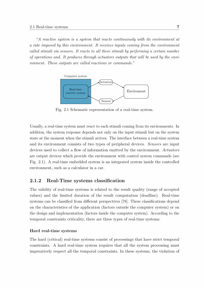
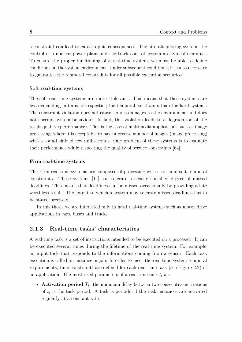
“A reactive system is a system that reacts continuously with its environment ata rate imposed by this environment. It receives inputs coming from the environmentcalled stimuli via sensors. It reacts to all these stimuli by performing a certain numberof operations and. It produces through actuators outputs that will be used by the envi-ronment. These outputs are called reactions or commands.”
Fig. 2.1 Schematic representation of a real-time system.
Usually, a real-time system must react to each stimuli coming from its environments. Inaddition, the system response depends not only on the input stimuli but on the systemstate at the moment when the stimuli arrives. The interface between a real-time systemand its environment consists of two types of peripheral devices. Sensors are inputdevices used to collect a flow of information emitted by the environment. Actuatorsare output devices which provide the environment with control system commands (seeFig. 2.1). A real-time embedded system is an integrated system inside the controlledenvironment, such as a calculator in a car.
2.1.2 Real-Time systems classification
The validity of real-time systems is related to the result quality (range of acceptedvalues) and the limited duration of the result computation (deadline). Real-timesystems can be classified from different perspectives [78]. These classifications dependon the characteristics of the application (factors outside the computer system) or onthe design and implementation (factors inside the computer system). According to thetemporal constraints criticality, there are three types of real-time systems:
Hard real-time systems
The hard (critical) real-time systems consist of processings that have strict temporalconstraints. A hard real-time system requires that all the system processing mustimperatively respect all the temporal constraints. In these systems, the violation of
8 Context and Problems
a constraint can lead to catastrophic consequences. The aircraft piloting system, thecontrol of a nuclear power plant and the track control system are typical examples.To ensure the proper functioning of a real-time system, we must be able to defineconditions on the system environment. Under subsequent conditions, it is also necessaryto guarantee the temporal constraints for all possible execution scenarios.
Soft real-time systems
The soft real-time systems are more “tolerant”. This means that these systems areless demanding in terms of respecting the temporal constraints than the hard systems.The constraint violation does not cause serious damages to the environment and doesnot corrupt system behaviour. In fact, this violation leads to a degradation of theresult quality (performance). This is the case of multimedia applications such as imageprocessing, where it is acceptable to have a precise number of images (image processing)with a sound shift of few milliseconds. One problem of these systems is to evaluatetheir performance while respecting the quality of service constraints [64].
Firm real-time systems
The Firm real-time systems are composed of processing with strict and soft temporalconstraints. These systems [14] can tolerate a clearly specified degree of misseddeadlines. This means that deadlines can be missed occasionally by providing a lateworthless result. The extent to which a system may tolerate missed deadlines has tobe stated precisely.
In this thesis we are interested only in hard real-time systems such as motor driveapplications in cars, buses and trucks.
2.1.3 Real-time tasks’ characteristics
A real-time task is a set of instructions intended to be executed on a processor. It canbe executed several times during the lifetime of the real-time system. For example,an input task that responds to the informations coming from a sensor. Each taskexecution is called an instance or job. In order to meet the real-time system temporalrequirements, time constraints are defined for each real-time task (see Figure 2.2) ofan application. The most used parameters of a real-time task ti are:
• Activation period Ti: the minimum delay between two consecutive activationsof ti is the task period. A task is periodic if the task instances are activatedregularly at a constant rate.

2.1 Real-time systems 9
• Release date ri: the earliest date on which the task can begin its execution.
• Start date si: it is also called the start execution date. It is the date on whichthe task starts its execution on a processor.
• End date ei: the date on which the task ends its execution on a processor.
• Execution time Ci: the required time for a processor to execute an instance ofa task ti. In general, this parameter is evaluated as the task worst case executiontime (WCET) on a processor. The WCET represents an upper bound of the taskexecution time. The value of this parameter should not be overestimated. Theproblem of estimating the task execution time has been extensively studied inthe literature [104, 106, 99, 113].
• Deadline Di: it corresponds to the date at which the task must complete itsexecution. Exceeding the due date (deadline) causes a violation of the temporalconstraints. we distinguish two types of deadlines:
- Relative deadline: Di the time interval between the task release date andits absolute deadline.
- Absolute deadline: the date at which the task must be completed (ri + Di).
Fig. 2.2 Real-time tasks’ characteristics.
Some parameters are derived from the basic parameters such as the utilizationfactor:
Ui = Ci
Ti.
Dynamic parameters are used to follow the behaviour of the task executions:
• rki : the release date of the kth task instance (tk
i ). In the periodic case, this datecan be calculated according to the task first release date r1
i :
rki = r1
i +(k−1) ·Ti

10 Context and Problems
• ski : the start date of the kth task instance (tk
i ).
• eki : the end date of the kth task instance (tk
i ).
• dki : the absolute deadline of the kth task instance (tk
i ). In the periodic case,this date can be computed in function of the relative deadline (Di) and the kthrelease date rk
i :
dki = rk
i +Di = r1i +(k−1) ·Ti +Di.
• Rki : the response time of the kth task instance (tk
i ). It is equal to eki − rk
i .
2.1.4 Tasks models
The real-time system environment defines the system temporal constraints. In otherwords, it defines the activation dates pace of the tasks. A task can be activatedrandomly (non-periodic) or at regular intervals (periodic). There are three classes ofreal-time tasks:
Periodic tasks
Tasks with regular arrival times Ti are called periodic tasks. A common use of periodictasks is to process sensor data and update the current state of the real-time system ona regular basis. Periodic tasks usually have hard deadlines, but in some applicationsthe deadlines can be soft. This class is based on the model of Liu and Layand [85].
Fig. 2.3 Liu and Layland model.
An example of Liu and Layland model is depicted in Figure 2.3. Each task ti ischaracterized by an activation period Ti, an execution time Ci (all instances of aperiodic task have the same worst case execution time Ci), a deadline Di, and eventually

2.1 Real-time systems 11
a release date (date of the first activation) ri. Each task instance must be executedentirely within the interval of length Ti. Successive executions of ti , admit periodicrelease dates and deadlines, where the period is equal to Ti.
Strictly periodic tasks is a particular case of this class. In addition to the Liu andLayland model, the task successive executions admit periodic start dates. In otherwords, the first instance (job) t1
i of task ti, which is released at r1i , starts its execution
at time s1i . Then, in every following period of ti, tk
i is released at rki and starts its
execution at ski . The kth release and start dates of ti can be written as follows:
rki = r1
i +(k−1) ·Ti
ski = s1
i +(k−1) ·Ti
In the following of the manuscript, r1i and s1
i are noted ri and si respectively.
Aperiodic tasks
An aperiodic task is a stream of instances arriving at irregular intervals. Aperiodictask has a relative deadline, with no activation dates and no activation periods. Thus,the task activation dates are random and can not be anticipated. These activations aredetermined by the arrival of events that can be triggered at any time such as messagefrom an operator. Several processes deal with this class of tasks as shown in [110].
Sporadic tasks
A sporadic task is an aperiodic task with a hard deadline and a minimum period pi [94].Two successive instances of a task must be separated by at least pi time units. Notethat without a minimum inter-arrival time restriction, it is impossible to guaranteethat a sporadic task’s deadline would always be met.
2.1.5 Execution mode
Multiple instances of a task can be executed during the lifetime of a real-time system.We distinguish two executions modes:
Non-preemptive mode
In non-preemptive execution mode, the scheduler cannot interrupt the task executionin favour of another one. In order to execute a new task, it is necessary to wait until
12 Context and Problems
the end of the current task. In other words, a task must voluntarily give it up thecontrol of the processor before the execution of an other task.
Preemptive mode
The difference between the non-preemptive execution mode and the preemptive oneis that the later gives the scheduler the control of the processor without the task’scooperation. According to the scheduling algorithm, the currently running task losescontrol of the processor when a task with higher priority is ready to be executedregardless of whether it has finished its execution or not.
In this thesis, we focus our study on modeling and scheduling applications composedof non-preempting strictly periodic tasks.
2.1.6 Communication constraints
Designers describe the embedded real-time systems workflow using block diagrams.These blocks correspond to functions that may be independent or dependent. Functionsare considered tasks as soon as they have been characterized temporally. Most of real-time applications require communication between tasks. This type of communicationconnects an emitting task to a receiving one. The emitting task produces data that areconsumed by the receiving task through a communication point. However, a receivingtask cannot consume a piece of data unless this data has been sent by the emittingtask. Thus, the execution of a receiving task should be preceded by the execution ofan emitting task, which imposes precedence constraints between some executions. Itshould be noted that the precedence constraint between executions (jobs) is mostlydue to the fact that both tasks are dependent. The dependency between the taskscan be described by a directed graph. The graph nodes represent the tasks and itsarcs represent the dependency relations between the tasks. There are two types ofdependencies:
• Dependencies that involve a loss of data. In this case, the receiving task can notconsume all the data produced by the emitting one. These data (which are notconsumed) have been overwritten by the newer data which are produced by morerecent emitting task executions. This is the case where the periods of dependenttasks correspond to prime numbers.
• Dependencies that do not involve a loss of data. In this case, the data producedby the emitting task executions are all consumed by the receiving task executions.

2.1 Real-time systems 13
In this thesis, we consider a communication mechanism between tasks which mayinvolve a loss of data. In other words, a task can be executed using the most recentdata of its predecessors. The description of the communication scheme betweenmulti-periodic tasks will be detailed in section 5.1 of chapter 5
2.1.7 Latency
Latency constraint between two tasks ti and tj is equivalent to impose that the gapbetween the end date of tj and the start date of ti does not exceed a certain value L.Limiting the time gap between these tasks guarantees that the response time - thetotal time required by a task in order accomplish its execution - of the second taskwill never exceed a preset critical value. Exceeding this value may lead to performancedegradation as well as instability of the system.
System latency evaluation
Real-time systems have to provide results to its environment in a timely fashion. Thisrequirement is typically measured by the duration (time gap) between an input eventarriving at the system input and its corresponding result events coming out from thesystem output. This time gap is denoted as the system latency. Executing a systemwith a long response time (fairly significant latency) may cause a lot of damages, suchas the late identification of an obstacle in an Advanced Driver Assistance Systems[117]. Depending on the application scenario, the system latency can be evaluatedwith different accuracy classes: worst-case latency, best-case latency, average latencyor different quantiles of latency.
In this thesis, we are interested in evaluating the worst-case system latency.
2.1.8 Multi-periodic systems
Complex real-time embedded systems should handle multiple distinct periods. This ismainly induced by the physical characteristic of sensors and actuators. A multi-periodicsystem is composed of a set of periodic tasks communicating with each other and havingdistinct periods. Each task is executed according to its own period. However, the entiresystem is executed according to a global period which is called the "hyper-period"(hp)[50]. This global period is equal to the Least Common Multiple (LCM) of all thesystem tasks periods. A task’s execution is called a Job or instance. The number ofthese instances (repetitions) can be computed according to the task period and thesystem hyper-period (hp
Ti). We distinguish two types of multi-periodic systems:
14 Context and Problems
Harmonic periodic system
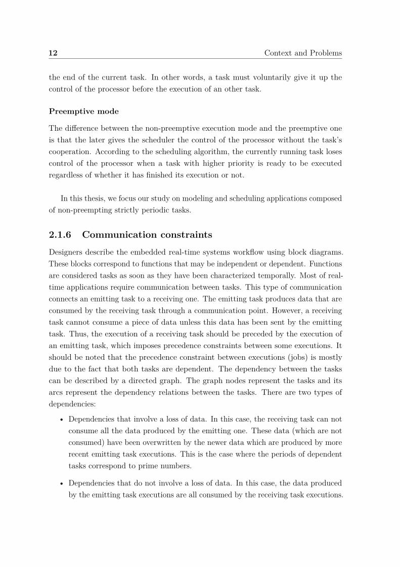
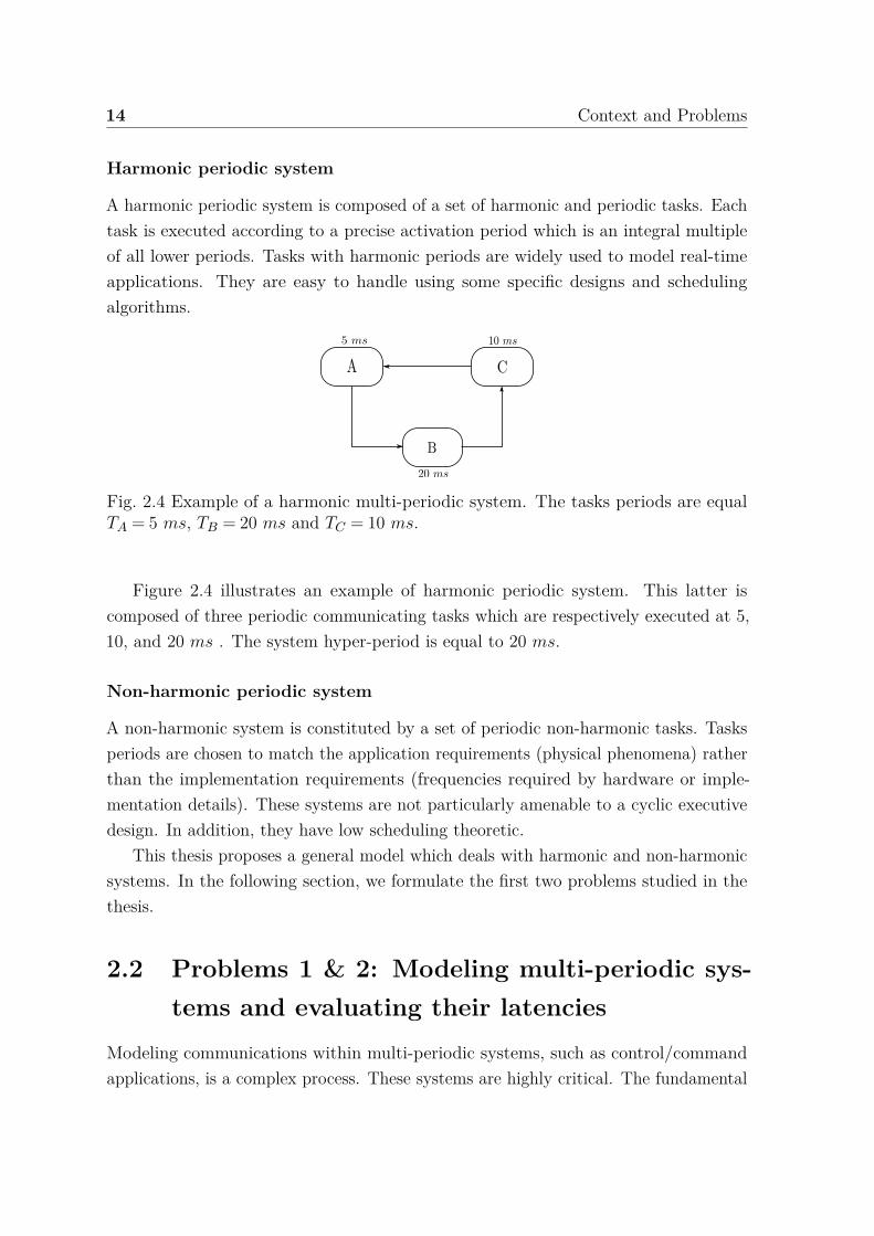
A harmonic periodic system is composed of a set of harmonic and periodic tasks. Eachtask is executed according to a precise activation period which is an integral multipleof all lower periods. Tasks with harmonic periods are widely used to model real-timeapplications. They are easy to handle using some specific designs and schedulingalgorithms.
Fig. 2.4 Example of a harmonic multi-periodic system. The tasks periods are equalTA = 5 ms, TB = 20 ms and TC = 10 ms.
Figure 2.4 illustrates an example of harmonic periodic system. This latter iscomposed of three periodic communicating tasks which are respectively executed at 5,10, and 20 ms . The system hyper-period is equal to 20 ms.
Non-harmonic periodic system
A non-harmonic system is constituted by a set of periodic non-harmonic tasks. Tasksperiods are chosen to match the application requirements (physical phenomena) ratherthan the implementation requirements (frequencies required by hardware or imple-mentation details). These systems are not particularly amenable to a cyclic executivedesign. In addition, they have low scheduling theoretic.
This thesis proposes a general model which deals with harmonic and non-harmonicsystems. In the following section, we formulate the first two problems studied in thethesis.
2.2 Problems 1 & 2: Modeling multi-periodic sys-tems and evaluating their latencies
Modeling communications within multi-periodic systems, such as control/commandapplications, is a complex process. These systems are highly critical. The fundamental

2.3 Modeling real-time systems 15
requirement is to ensure the system functionality with respect to the data exchangebetween its parts as well as their temporal constraints. These systems require adeterministic behaviour, which means that for a given input the system execution mustproduce the same output. In addition, the system’s execution must be temporallydeterministic as well, always having the same temporal behaviour and respecting severalhard real-time constraints.
Data flow models are a class of formalisms used to describe in a simple and compactway the communications of regular applications (for example video encoders). A modelof this class is usually represented in the form of a network of communicating taskswhere their executions are guided by the data dependencies. In this context, the firstproblem addressed in this thesis is:
How can we model the communications within multi-periodic systems,while meeting simultaneously their temporal and data requirements?
The second problem of this thesis is:
How can we evaluate the latency of a multi-periodic system?
We detail in chapter 4 the state of the art of modeling multi-periodic systems andevaluating their latencies using data flow formalisms. Next section lists several researchapproaches of modeling real-time systems.
2.3 Modeling real-time systemsReal-time systems are continuously interacting with external environment (othersystems or hardware components). Assurance of a global quality of this kind ofinteractions is a major issue in the systems design. Nowadays, it is widely acceptedthat modelling plays a central role in the systems engineering. Modeling real-timesystems provides an operational representation of the system overall organization aswell as the behaviour of all its sub-systems. Therefore, using models can profitablysubstitutes experimentation. Modeling advantages can be summarized as follows [107]:
• flexibility : the model and its parameters can be modified in a simple way;
• generality by using abstraction: solving the scale factor issue;

16 Context and Problems
• expressibility: improving observation, control and avoidance perturbations dueto experimentation;
• predictability: real-time system characteristics can be predictable such as thesystem latency;
• reduced cost: systems modeling is less expensive than real implementation interms of time and effort.
2.3.1 Models for Real-Time Programming
In general, the time representations in a real-time system can be classified into threetypes [74]: asynchronous, timed and synchronous models. These time models differmainly in the manner of characterizing the correlated behaviour of a real-time system.More precisely, the time models define the relationship between the physical-timeand logical-time which depends on several factors, such as the execution platformperformance and utilization, the scheduling policies, the communication protocols aswell as the program and compiler optimization.
Asynchronous model
Fig. 2.5 Execution of an asynchronous model. Logical-time ≤ Physical-time.
Asynchronous model is a classical representation of real-time programming [118] suchas the real-time programming languages “Ada” or “C”. Applications are representedby a finite number of processes (tasks). Logical-time in the asynchronous modelcorresponds to the task’s processing time (see Figure 2.5). The system execution iscontrolled by a scheduler setting the execution dates of the application’s tasks. A task’sexecution depends on the adopted scheduling policy within the Real-Time Operating

2.3 Modeling real-time systems 17
System (RTOS in short). Accordingly, in asynchronous model the logical-time is nota priori determined and may vary depending on several factor such as the platformperformance or the scheduling scheme. Therefore, asynchronous model logical-timevariation is constrained by real-time deadlines: logical-time must be less than or equalto physical-time. The system schedulability condition (i.e. all deadlines are met) mustbe indicated in the scheduling scheme of real-time operating system. A schedulabilityanalysis also requires the analysis of the worst-case execution times.
Timed model
The principle of timed model is based on the idea that interactions between twoprocesses can only occur at two precise moments τ and τ
′ . The interval between thesemoments (]τ,τ
′ [) is a fixed non-zero amount of time which corresponds to the logicalduration of computation and communication between two processes (see Figure 2.6).
Fig. 2.6 Execution of a timed model. Logical-time = Physical-time.
In this context, programmers annotate their programs describing real-time systemswith logical durations. The latter are an approximation of the actual computation andcommunication times. In this case, logical-time and physical-time are equal. Unlike theasynchronous model, since all the necessary information are known before execution,verification of some properties related to the logical temporal behaviour of the systembecomes possible. For example, a scheduling validity or the system latency evaluationcan be checked using a static method at compile-time.
In the timed model the program’s logical execution time is fixed, two situationsmay arise at the execution level:
• The program may not have finished executing while its logical execution timeis exceeded. If the timed program is indeed late, a runtime exception may bethrown (an exception is usually generated).
18 Context and Problems
• The program may have completed its execution before its logical delay expiration.If the timed program finishes early, its output is delayed until the specified logicalexecution time has elapsed. The model annotation values should be carefullychosen in order to reduce the phase shift between the computations and outputproductions.
The timed model is well-suited for embedded control systems, which require timingpredictability. The timed programming language Giotto [61] supports the designand implementation of embedded control systems [75], in particular, on distributedhardware. The key element in Giotto is that timed tasks are periodic and deterministicwith respect to their inputs and states. The logical execution time of a Giotto taskis the period of the task. For example, a 10Hz Giotto task runs logically for 100msbefore its output becomes available and its input is updated for the next invocation.
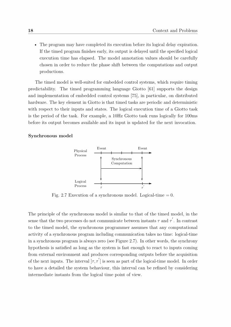
Synchronous model
Fig. 2.7 Execution of a synchronous model. Logical-time = 0.
The principle of the synchronous model is similar to that of the timed model, in thesense that the two processes do not communicate between instants τ and τ
′ . In contrastto the timed model, the synchronous programmer assumes that any computationalactivity of a synchronous program including communication takes no time: logical-timein a synchronous program is always zero (see Figure 2.7). In other words, the synchronyhypothesis is satisfied as long as the system is fast enough to react to inputs comingfrom external environment and produces corresponding outputs before the acquisitionof the next inputs. The interval ]τ,τ
′ [ is seen as part of the logical-time model. In orderto have a detailed the system behaviour, this interval can be refined by consideringintermediate instants from the logical time point of view.

2.3 Modeling real-time systems 19
In order to model the communications within multi-periodic systems, we character-ized the systems behavior using a temporal approach (a timed model). We assumethat all the tasks parameters are provided by the developer.
2.3.2 Low-level languages
A large real-time systems class is implemented using low-level languages. However, theuse of these languages presents several major disadvantages:
• Time-triggered communications are hard to implement. In fact, a part of thesystem should be scheduled manually.
• A basic mechanism for tasks communications is the “rendez-vous”, which isimplemented by three primitive operations: send, receive and reply. This typeof communications may lead to deadlocks such as two communicating tasks arewaiting each other to resume their executions.
• A low level of abstraction makes the program correctness harder to verify (manu-ally or using automated tools).
• The use of low-level languages makes the program maintenance difficult. This isdue to lack of informations differentiating parts of the program correspondingto real design constraints and parts which only correspond to implementationconcerns.
Dealing with such considerations cannot be avoided. Actually, real-time systemsdevelopers tend to use programming languages with a higher-level of abstraction, wherethese issues are managed by the language compiler. Several languages seek to coverthe entire process (from verification up to implementation). Their approach is basedon translating the input program modeled with a high-level language into a low levelcode using automatic code generation processes. Such a strategy reduces the requiredtime for implementation. Then, it provides a simple system description which is easierto analyse using verification tools. Finally, the compilation ensures the low-level codecorrectness.
2.3.3 Synchronous languages
The synchronous approach presents a high level of abstraction. This approach is basedon simple and solid mathematical theories, which ease the program implementation
20 Context and Problems
and verification. Synchronous approach introduces a discrete and logical time conceptdefined as succession of steps (instants). Each step corresponds to the system reaction.The synchrony assumption consider that the system is fast enough to react to itsenvironment stimulus. This practically means that the system changes occurringduring a step are treated at the next step and implies that responsiveness and precisionare limited by the step duration.
The synchronous execution model has been developed in order to control in deter-ministic way reactions and interactions with the external environment. Esterel [16],Lustre [56] and Signal [13] are examples of synchronous languages. In order to meetthe synchrony assumption, the correct implementation of these languages requires theestimation of the worst case execution times of the program code.
Lustre
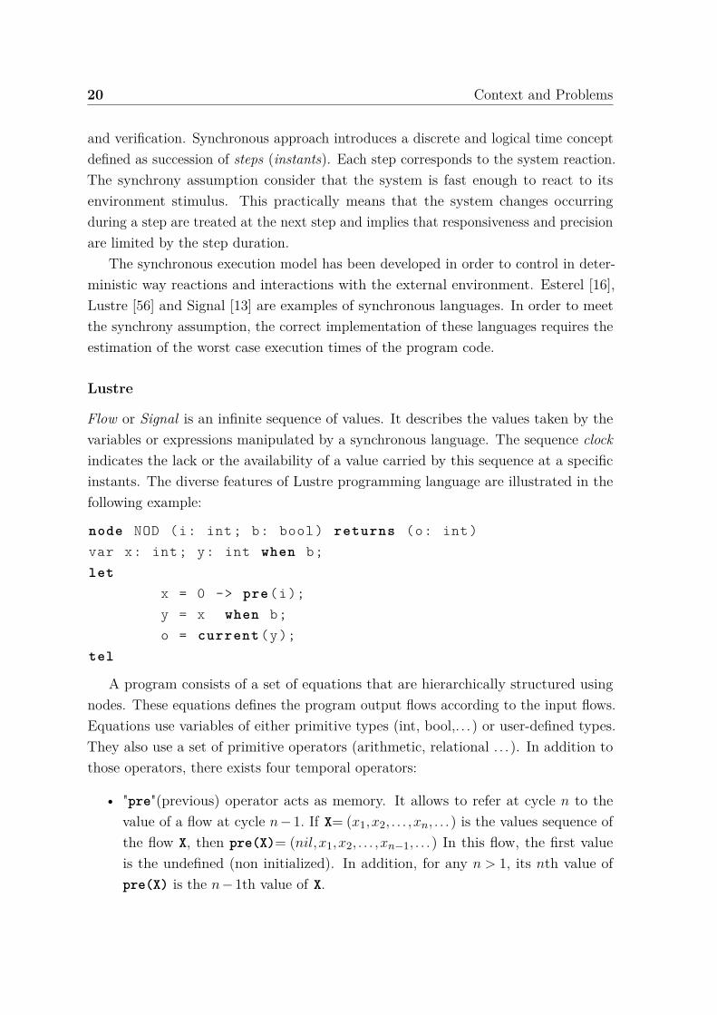
Flow or Signal is an infinite sequence of values. It describes the values taken by thevariables or expressions manipulated by a synchronous language. The sequence clockindicates the lack or the availability of a value carried by this sequence at a specificinstants. The diverse features of Lustre programming language are illustrated in thefollowing example:
node NOD (i: int; b: bool) returns (o: int)var x: int; y: int when b;let
x = 0 -> pre(i);y = x when b;o = current (y);
tel
A program consists of a set of equations that are hierarchically structured usingnodes. These equations defines the program output flows according to the input flows.Equations use variables of either primitive types (int, bool,. . .) or user-defined types.They also use a set of primitive operators (arithmetic, relational . . .). In addition tothose operators, there exists four temporal operators:
• "pre"(previous) operator acts as memory. It allows to refer at cycle n to thevalue of a flow at cycle n−1. If X= (x1,x2, . . . ,xn, . . .) is the values sequence ofthe flow X, then pre(X)= (nil,x1,x2, . . . ,xn−1, . . .) In this flow, the first valueis the undefined (non initialized). In addition, for any n > 1, its nth value ofpre(X) is the n−1th value of X.

2.3 Modeling real-time systems 21
• "->"(follow by) operator is used to initialize a flow. If X = (x1,x2, . . . ,xn, . . .) and Y= (y1,y2, . . . ,yn, . . .) are two flows of the same type, then X -> Y= (x1,y2, . . . ,yn, . . .).This means that X -> Y is equal to Y except the first value.
• "when" operator is used to create a slower clock according to a boolean flow suchas B = (true,false, . . . , true, . . .). X when B is the flow whose clock tick when Bis true and its values are equal to those of X at these instants.
• "current" operator is used to get the current value which is computed at thelast clock tick of the flow. If Y = X when B is a flow, then current(Y) is a flowhaving the same clock as B and whose value at a given clock’s tick is the valuetaken by X at the last clock’s tick when B was true.
i 1 2 3 4 5 . . .b true true false false true . . .
pre(i) nil 1 2 3 4 . . .x = 0 -> pre (i) 0 1 2 3 4 . . .
y = x when b 0 1 4 . . .o = current(y) 0 1 1 1 4 . . .
Table 2.1 Lustre program behaviour.
The Lustre program behaviour is depicted in table 2.1. The flow value is givenat clock’s tick. The node output (o) is computed according to the inputs (i,b). xand y are two local (intermediate) variables. x = 0 -> pre (i) equation sets x to 0initially, and the subsequent x is equal to the value of i at the previous clock’s tick. y= x when b means that y is present only when b is true and it takes the value of xat this instant. Finally, the output o is defined as the current value of y when it wasavailable.
Due to the complexity of high-performance applications and to the intrinsic combi-natorics of synchronous execution, multiple clock domains have to be considered atthe application level. This is the case of a single system with multiple input/outputassociated with several real-time clocks. In this context, we focussing our study onmodelling multi-periodic systems. In the following part, we introduce two synchronouslanguages dedicated to model multi-periodic systems.
Lucy-n
Synchronous languages such as Lustre [56] or Lucid Synchrone [103] define a restrictedclass of Kahn Process Networks which can be executed without buffers. For some appli-

22 Context and Problems
cations (real-time streaming applications), synchrony condition forces the programmerto implement manually complex buffers, which is very error-prone. In order to avoidthis issue, Cohen et al. [27] generalized the synchronous approach by introducing then-synchronous approach. This latter is based on defining a relaxed clock-equivalence.Communication between n-synchronous streams is implemented with a buffer of size n.Accordingly, quantitative information about clocks can be revealed so that the compilercan decide whether it is possible to buffer a stream into another or not.
Based on the n-synchronous approach, Mandel et al. [89] introduced Lucy-n anextension of Lustre with a build-in buffer operator. The purpose of this language is torelax synchrony constraints while ensuring determinism and execution in bounded timeand memory. Lucy-n handles the communication between processes of different ratesthrough the buffers. A clock analysis is used to determine where finite buffers must beintroduced into the data flow graph. Finally, clocks and buffer sizes are computed bythe compiler.
In this thesis, tasks parameters are extracted from the real-time application itself.In addition, communication between two periodic tasks are modeled using an non-flow-preserving semantics.
Prelude
Prelude [42, 41] is a real-time programming language inspired by Lustre [56]. It focuseson the real-time aspects of multi-periodic systems. Predule is an integration languagethat assembles local mono-periodic programs into a globally multi-periodic system.
A program consists of a set of equations, structured into nodes. Real-time constraintsrepresenting the environment requirements are specified either on nodes’ inputs/outputs(e.g. periods, deadlines) or on nodes (worst-case execution time). Equations of anode define its output flows according to its input flows. In order to manage thecommunication between nodes with different rates, transition operators are addedto the synchronous data flow model. These operators are formally defined usingstrictly periodic clocks. They accelerate, decelerate, or offset flows. Therefore, theyallow the definition of communication patterns provided by the user. The transitionoperators in Prelude allow the oversampling data sent from lower frequency tasks andunder-sampling data sent from higher frequency tasks. Consequently, communicationsbetween nodes are non-flow-preserving (quasi-synchrony approach [23]).
The compiler translates a Prelude program into a set of communicating periodictasks that respect the semantics of the original program. The tasks set is implementedas concurrent “C” threads that can be executed on a standard real-time operating
2.3 Modeling real-time systems 23
system. In case of a mono-processor platform [43], Prelude compiler implementsdeterministic communications between tasks without synchronization mechanisms. Inorder to establish these communications, the compiler ensures that the producer writebefore the consumer reads. In addition, it prevents a new execution of the producerto overwrite the value of its previous execution, if this latter is still required by otherexecutions. Tasks parameters (release dates and deadlines) were adjusted in order tobe scheduled on a mono-processor using Earliest Deadline First policy [85].
Our approach differs from [42, 41] in the following points: we characterize thesystems behavior using a temporal approach (a timed model), in order to model thecommunications of multi-periodic systems. In addition, we tackle the mono-processorscheduling problem for applications modeled as non-preemptive strictly periodic tasks.Unfortunately, it has been proven [45] that the schedulability conditions for preemptivescheduling become, at best, necessary conditions for the non-preemptive case.
2.3.4 Oasis
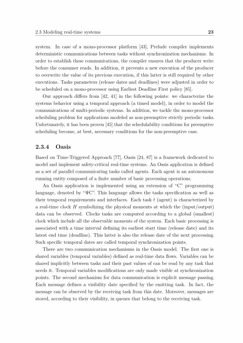
Based on Time-Triggered Approach [77], Oasis [24, 87] is a framework dedicated tomodel and implement safety-critical real-time systems. An Oasis application is definedas a set of parallel communicating tasks called agents. Each agent is an autonomousrunning entity composed of a finite number of basic processing operations.
An Oasis application is implemented using an extension of “C” programminglanguage, denoted by “ΨC”. This language allows the tasks specification as well astheir temporal requirements and interfaces. Each task t (agent) is characterized bya real-time clock H symbolizing the physical moments at which the (input/output)data can be observed. Clocks tasks are computed according to a global (smallest)clock which include all the observable moments of the system. Each basic processing isassociated with a time interval defining its earliest start time (release date) and itslatest end time (deadline). This latter is also the release date of the next processing.Such specific temporal dates are called temporal synchronization points.
There are two communication mechanisms in the Oasis model. The first one isshared variables (temporal variables) defined as real-time data flows. Variables can beshared implicitly between tasks and their past values of can be read by any task thatneeds it. Temporal variables modifications are only made visible at synchronizationpoints. The second mechanism for data communication is explicit message passing.Each message defines a visibility date specified by the emitting task. In fact, themessage can be observed by the receiving task from this date. Moreover, messages arestored, according to their visibility, in queues that belong to the receiving task.
24 Context and Problems
Our communication model is similar the temporal variable mechanism in thesense that data is available at the emitting task deadline and can only consumed(received) at release date of the receiving task. However, in our model the releasedates and the deadlines of successive executions do not necessary coincide. In addition,communications between the tasks executions is modeled, in a deterministic way, usinga Synchronous Data Flow Graph whose size is equal to the application size.
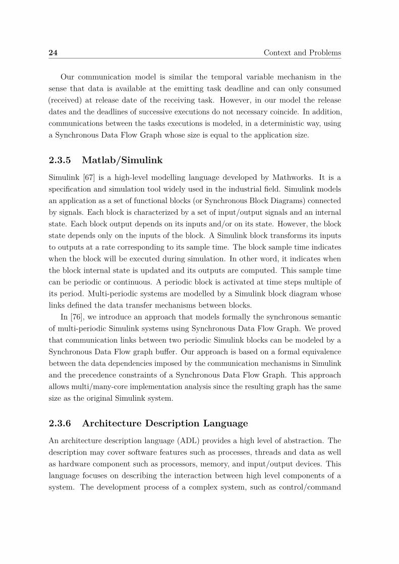
2.3.5 Matlab/Simulink
Simulink [67] is a high-level modelling language developed by Mathworks. It is aspecification and simulation tool widely used in the industrial field. Simulink modelsan application as a set of functional blocks (or Synchronous Block Diagrams) connectedby signals. Each block is characterized by a set of input/output signals and an internalstate. Each block output depends on its inputs and/or on its state. However, the blockstate depends only on the inputs of the block. A Simulink block transforms its inputsto outputs at a rate corresponding to its sample time. The block sample time indicateswhen the block will be executed during simulation. In other word, it indicates whenthe block internal state is updated and its outputs are computed. This sample timecan be periodic or continuous. A periodic block is activated at time steps multiple ofits period. Multi-periodic systems are modelled by a Simulink block diagram whoselinks defined the data transfer mechanisms between blocks.
In [76], we introduce an approach that models formally the synchronous semanticof multi-periodic Simulink systems using Synchronous Data Flow Graph. We provedthat communication links between two periodic Simulink blocks can be modeled by aSynchronous Data Flow graph buffer. Our approach is based on a formal equivalencebetween the data dependencies imposed by the communication mechanisms in Simulinkand the precedence constraints of a Synchronous Data Flow Graph. This approachallows multi/many-core implementation analysis since the resulting graph has the samesize as the original Simulink system.
2.3.6 Architecture Description Language
An architecture description language (ADL) provides a high level of abstraction. Thedescription may cover software features such as processes, threads and data as wellas hardware component such as processors, memory, and input/output devices. Thislanguage focuses on describing the interaction between high level components of asystem. The development process of a complex system, such as control/command
2.3 Modeling real-time systems 25
application, can be supported by such approach. The software engineering communityuses ADLs in order to describe the software architectures. ADLs advantages are:
- Providing a formal representation of architectures.
- Both human and machines can apprehend their designs.
However, ADLs have a major drawback. There is no universal agreement on whatADLs should represent, especially when it is about the system behaviour.
In the sequel, we describe two languages dedicated to model multi-periodic systems.
Architecture Analysis and Design Language
Architecture Analysis and Design Language (AADL) [40] is used to model the softwareand hardware architecture of a real-time embedded system. An AADL design consistsof a set of components interacting through interfaces. Components can be separatedinto three categories: application software (process, thread, etc.), execution platform(hardware) or composite components (composition of other components).
In AADL, user can specify a set of properties and extend them in order to fulfilhis own requirement. For instance, a variety of execution properties can be assignedto threads, including timing (such as worst case execution times), dispatch protocols(such as aperiodic, periodic), memory size, etc.
Interactions among components are represented through connections defined be-tween interface elements. Communication mechanisms can either be immediate (be-tween simultaneous dispatches of the communicating threads) or delayed (from thecurrent dispatch of the sender to the next dispatch of the receiver). Immediate com-munications impose a precedence order from the data sender to the receiver. However,in delayed communications, data are available to a receiving thread is that valueproduced at the most recent deadline of the emitting thread. Immediate and delayedcommunications can also be established between threads of different periods.
The AADL approach allows to model multi-periodic systems with a high-level ofabstraction. The main restriction of this approach is that it provides a limited choice ofcommunication schemes. However, our approach allows the definition of several (user-provided) communication schemes, while relying on the solid mathematical backgroundof the SDFGs.
GIOTTO
Giotto [62] is a time-triggered Architecture Description Language designed to implementreal-time systems. These latter can be executed in a distributed environment. A Giotto

26 Context and Problems
program allows to specify the possible interactions systems’ components and theirenvironment.
A Giotto program is composed of four major concepts:
- Tasks: Giotto tasks are periodic. They are executed at regularly spaced pointsin time. They express calls to functions and they can have parameters definedby input and output ports.
- Ports: They allow the communication between a system and its environment.There are three types of ports: input, output and private. Private ports are usedto communicate between tasks.
- Modes: They represent the major elements of a Giotto program. Giotto can onlybe in one mode at a certain instant. A mode consists of a period, an output set,actuators update, tasks execution and a set of switch modes.
- Drivers: They are functions that provide values for the input ports from sensorsand mode ports. Drivers can be guarded: the guard of a driver is a predicateon sensor and mode ports. In other words, a task is executed only if the driverguard is true. Otherwise, the task execution is skipped.
A Giotto program consists of a set of modes. Each mode repeats the execution of afixed set of tasks. These tasks are multi-periodic: each mode has a period P and eachtask has a frequency f , thus the task period is given by P
f .
Data produced by a task are available only at the end of its period. Conversely,when a task is executed it consumes only the last inputs’ values, which is produced atthe beginning of its period. This communication implies significant latencies betweeninput data and the corresponding output one. However, our communication modelconsiders that the data are available at the task deadline instead of the end of the taskperiod (Di ≤ Ti).
2.4 Scheduling real-time systemReal-time scheduling problem consists in defining the tasks’ execution order on pro-cessors of a given architecture. In real-time systems, tasks are subject to temporalconstraints and possibly other constraints. The scheduling purpose is to set a start(preemption/recovery) date for each task execution in order to respect the systemconstraints.

2.4 Scheduling real-time system 27
A scheduler provides a policy for ordering the tasks executions on processorsaccording to some predefined criteria. A scheduler is said to be optimal with respectto a given class of schedulers if and only if it generates a valid schedule for any feasibletask set in this class [45]. In other words, a scheduling algorithm is said to be optimalregarding a system and a task model if it can schedule all tasks’ sets that comply withthe task model and are feasible on the system [33]. We distinguish several schedulingclasses:
Offline and online scheduling
A scheduling is offline if all the decisions are made at compile-time (before the applica-tion execution). A table is generated containing the scheduling sequence that will berepeated infinitely during run-time. In order to be efficient, this approach requires apriori knowledge of all tasks parameters. Therefore, this approach is workable onlyif all the tasks are actually periodic. This approach is static and does not adapt toenvironment changes. However, offline scheduling is often the only way to predictwhether temporal constraints are satisfied or not in a complex real-time system. Asthe scheduling is offline, the use of exact algorithms is possible even if these methodsare very time consuming.
A scheduling is online if decisions are made during the runtime of the system. Ateach moment of the system life time, the scheduling algorithm is able to process tasksthat have not been previously activated using the task parameters specific to thismoment. This makes online scheduling flexible and able to adapt to environmentchanges. In this case, the use of effective heuristics is preferred to that of optimalalgorithms.
Independent/dependent tasks Scheduling
The scheduling policy is divided into dependent and independent tasks scheduling.Tasks whose execution is not dependent upon other tasks’ executions are termedindependent tasks. These latter have no dependencies among the tasks and haveno precedence order to be followed during scheduling. In this case, we talk aboutindependent tasks scheduling.
Given a real-time system, dependency between tasks ensures that the tasks areexecuted in some order. Executing a dependent task may require the availability ofdata provided by other tasks of the system. Therefore, this task can only be schedule

28 Context and Problems
after the compilation of its predecessors. The relationship between independent tasksis typically described by a directed graph called precedence or communication graph.
Preemptive and non-preemptive scheduling
A scheduling is called preemptive if the task’s execution can be suspended and resumedlater on without affecting its behaviour, except by increasing its elapse time. A task istypically suspended by an other task with higher priority, when this latter becomesready to be executed. Additional cost caused by the preemption may not be negligiblecompared to the tasks execution and communication times. Moreover, the system mayinclude critical sections where preemption is not allowed.
In contrast, a non-preemptive scheduler does not suspend tasks. When a task isselected to be executed, it runs until the end of its execution. In this case, a higherpriority task cannot interrupt the execution of a lower priority task even when it becomesready to be executed. Compared to preemptive scheduling, non-preemptive algorithmsare easy to implement and have a low runtime overhead. The time consumption ofeach task in the system can be easily characterized and predicted [65]. Even thoughthe non-preemptive scheduling has been proven to be NP-Hard in strong sense [80],this type of scheduling is widely used in industrial applications such as cell phonedevices [100] and mobile robotics [101].
Mono-processor and Multi-processor scheduling
Designing real-time systems is influenced by the hardware architecture on which theapplication may run. It designates the physical resources needed to control the process.This architecture is composed of processors, input / output cards, memories, networks,etc. According to the processors number, we distinguish two scheduling problems:
- Mono-processor scheduling: All the system tasks are executed by a single proces-sor.
- Multi-processor scheduling: In order to be executed, the application’s tasks areassigned to n processors sharing a central memory.
In the following section, we formulate the scheduling problem studied in the thesis.

2.5 Problem 3: Scheduling strictly multi-periodic system with communicationconstraints 29
2.5 Problem 3: Scheduling strictly multi-periodicsystem with communication constraints
Nowadays, real-time embedded systems are becoming increasingly complex. Conse-quently, these systems require additionally Real-Time Operating Systems (RTOS inshort) to manage concurrent tasks and critical resources. Most RTOS implementreal-time dynamic scheduling strategies such as Rate Monotonic, Earliest DeadlineFirst and so on. The real-time applications are modeled as a set of periodic tasks. Eachtask is characterized by a set of parameters such as period, release date, deadline and soon. Several schedulability conditions have been provided by the real-time community.These conditions verify, prior to the implementation phase, whether a set of tasks willmeet their deadlines for a given scheduling strategy and platform.
Several studies addressed the preemptive scheduling problem of periodic tasks set.However, much less attention was given to the non-preemptive one. In fact, preemptivescheduling has a good task responsiveness, however it increases the resource utilizationrate compared to non-preemptive scheduling. Nonetheless, there exists several caseswhere non-preemptive scheduling is preferable. For instance, the overhead generated bypreemption is not always negligible compared to task execution time and inter-processorcommunication. Non-preemptive scheduling on a uniprocessor guarantees exclusiveaccess to shared resources and data as well as eliminating the need for synchronizationand associated overhead. On the other hand, many industrial applications (e.g. avionicapplications [1]) are modeled as a set of strictly periodic tasks. This strict periodicity isusually essential to avoid problems arising form input and output jitters. For example,input jitter can cause a data loss from sensors. Output jitter may lead to performancedegradation of the systems, as its negligence can be a source of instability.
On the other hand, communication within multi-periodic systems is more and moreindispensable. Due to the tasks strict deadlines that must be met, communicationsbetween the tasks executions are implemented in a completely deterministic manner.In this context, the third problem we address in this thesis is:
How to schedule on mono-processor a set of strictly periodic tasks, as-suming that these tasks communicate with each other and can not be pre-empted?
We detail in chapter 4 the state of the art regarding this scheduling problem.
30 Context and Problems
2.6 ConclusionIn this chapter, we introduced the context of this thesis. We presented an overview ofreal-time systems and their characteristics. We have formulated the two first problemsthat we studied in this thesis: modeling communications within multi-periodic systemsand evaluating their latencies. In addition, we have reviewed several existing approachesregarding multi-periodic systems design. The novelty of our approach consists in usingSynchronous Data Flow Graphs for modeling communications within multi-periodicsystems in a deterministic way. Afterwards, we have introduced the basic notionsof real-time scheduling. Finally, we formulated the third problem studied in thisthesis: mono-processor scheduling of non-preemtive strictly periodic set of tasks withcommunication constraints.
The following chapter introduces an overview of data flow models. Moreover, itintroduces notions and transformations related to the Synchronous Data Flow Graphs.
Chapter 3
Data Flow models
The emergence of microelectronics and modern calculators led to the development ofincreasingly accurate models. These models seek to formally describe the notion ofparallel and distributed computing. Kahn Process Network is one of the first attemptswhich models an application using First In First Out queues between the applicationsub-parts. However, this model is too permissive to allow an algorithmic prediction ofthe application performances. Nowadays, Synchronous Data Flow graph is a widelyused model which provides a compromise between the application expressiveness andanalyse.
This chapter provides an overview of data flow models and introduces importantnotion concerning them. Section 3.1 presents an overview of data flow models. Section3.2 introduces notions and transformations related to Synchronous Data Flow Graphmodel. Section 3.3 concludes the chapter.
3.1 Data Flow GraphsThe data flow model is inspired from computation graphs and Kahn Process Networks(KPN). This model is based on a graphical representation of programs and architectures.In the model’s original definition [34, 32], the graph vertices represent the elementaryoperations of the computer program and the graph edges between two vertices modelthe data dependencies between two operations. The program’s initial conditions aremodeled by adding tokens on the graph edges. In Denis’ model [34], an operationwhich is represented by a graph vertex, can be executed whenever data are available onall its inputs. When an operation is executed, it consumes a token on each input edgeand produces a token on each output edge. The data flow representation is dedicatedto computer programs, multi-processors architecture and parallel compilation.

32 Data Flow models
In the sequel, we present data flow models that are frequently used for embeddedsystems design. These models are: Kahn Process Network, Computation Graph,Synchronous Data Flow Graph and Cyclo-Static Data Flow Graph.
3.1.1 Kahn Process Network
We start by presenting Kahn Process Network (KPN in short) [46] since it is one ofthe most general data flow model. KPN is a data flow model based on a graphicaldescription. It describes an application using a directed graph. the vertices symbolizethe application sub-sections (processes). During the application execution, processescommunicate through communication channels. These channels are unbounded FIFO(First In First Out) buffers which temporarily store data. The input process canexclusively write into the buffer and the output process can exclusively read fromthe buffer. Reading from an empty buffer is blocking. In fact, when a process startsreading from a buffer, its execution is suspended until the data arrival (it must waitfor the data availability before resuming its execution). The process cannot verify thepresence of data before its execution. In addition, the processes are not reentrant.This means when a process starts executing, it must finish before starting an otherexecution.
ti tj. . . . . .
Fig. 3.1 Example of Kahn Processor Network.
The Kahn Process Network is a deterministic model. Indeed, the output data ofthe KNP depend only on the input data. This output value is neither influenced bythe processes execution times and their executions order nor by the communicationdelays between them. Moreover, the semantic of this model does not allow the buffersizing. In order to compensate this issue, the buffer has infinite size. Thus, this modelis useful to describe complex applications. However, it is unable to predict the systemperformances.
3.1.2 Computation Graph
Computation graphs [69] (CG in short) are one of the first static data flow model. Karpand Miller defined the CG in order to propose an alternative to sequential execution

3.1 Data Flow Graphs 33
model. As the Kahn Process Network, an application (system) is represented bydirected graph. The graph nodes model the tasks (or sub-tasks) of an application. Thegraph arcs represent the data exchange between these tasks. Each arc correspondsto an unbounded FIFO (First In First Out) buffer connecting an input task to anoutput one. At the end of the input task execution, a fixed amount of data is producedand stored temporarily in the buffer. According to a fixed threshold, these data aresubsequently consumed from the buffer at the beginning of the output task execution.Each task activation depends only on the availability of a sufficient amount of data onall of its input arcs. In addition, each buffer may contain an initial amount of data.
ti
3tj
7 : 4. . . . . . 2
Fig. 3.2 Example of Computation Graph.
In the sequel, we referred data as tokens. Figure 3.2 represents a ComputationGraph consisting of two tasks ti and tj connected by a buffer a = (ti, tj). The initialamount of tokens is equal to 2. Each execution of ti produces 3 tokens in the buffer a.In order to be able to execute, tj must wait for the availability of 7 tokens in the buffer,since the required data threshold is equal to 7. At the beginning of its execution, tj
consumes 4 tokens from the buffer a. Note that the data threshold must be greater orequal than the amount of tokens consumed by tj .
Some applications are represented using the Computations graphs model whichhighlights the parallelism between their different parts. Karp and Miller [69] show thatthe execution of a program modeled by a CG is deterministic (static). It is possibleto study the program behaviour even without its execution. Accordingly, severalfundamental problems become decidable such as checking the application liveliness(absence of deadlock).
3.1.3 Synchronous Data Flow Graph
The “Synchronous Data Flow Graphs” (SDFG in short) are a formalism introducedand studied by Lee and Messerchmidtt [83, 84] in order to model the communicationswithin an embedded applications. They are defined by a set of tasks exchangingdata using FIFO queues. A SDFG is represented by an oriented graph G = (T ,A).SDFGs can be considered as a particular case of Computation Graphs where the datathresholds of the buffers are equal to the consumption rates.
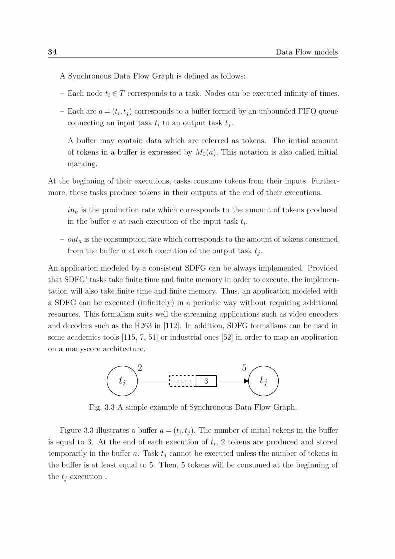
34 Data Flow models
A Synchronous Data Flow Graph is defined as follows:
– Each node ti ∈ T corresponds to a task. Nodes can be executed infinity of times.
– Each arc a = (ti, tj) corresponds to a buffer formed by an unbounded FIFO queueconnecting an input task ti to an output task tj .
– A buffer may contain data which are referred as tokens. The initial amountof tokens in a buffer is expressed by M0(a). This notation is also called initialmarking.
At the beginning of their executions, tasks consume tokens from their inputs. Further-more, these tasks produce tokens in their outputs at the end of their executions.
– ina is the production rate which corresponds to the amount of tokens producedin the buffer a at each execution of the input task ti.
– outa is the consumption rate which corresponds to the amount of tokens consumedfrom the buffer a at each execution of the output task tj .
An application modeled by a consistent SDFG can be always implemented. Providedthat SDFG’ tasks take finite time and finite memory in order to execute, the implemen-tation will also take finite time and finite memory. Thus, an application modeled witha SDFG can be executed (infinitely) in a periodic way without requiring additionalresources. This formalism suits well the streaming applications such as video encodersand decoders such as the H263 in [112]. In addition, SDFG formalisms can be used insome academics tools [115, 7, 51] or industrial ones [52] in order to map an applicationon a many-core architecture.
ti
2tj
5. . . . . . 3
Fig. 3.3 A simple example of Synchronous Data Flow Graph.
Figure 3.3 illustrates a buffer a = (ti, tj). The number of initial tokens in the bufferis equal to 3. At the end of each execution of ti, 2 tokens are produced and storedtemporarily in the buffer a. Task tj cannot be executed unless the number of tokens inthe buffer is at least equal to 5. Then, 5 tokens will be consumed at the beginning ofthe tj execution .
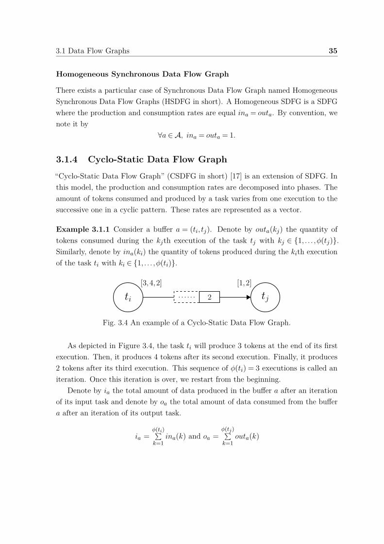
3.1 Data Flow Graphs 35
Homogeneous Synchronous Data Flow Graph
There exists a particular case of Synchronous Data Flow Graph named HomogeneousSynchronous Data Flow Graphs (HSDFG in short). A Homogeneous SDFG is a SDFGwhere the production and consumption rates are equal ina = outa. By convention, wenote it by
∀a ∈ A, ina = outa = 1.
3.1.4 Cyclo-Static Data Flow Graph
“Cyclo-Static Data Flow Graph” (CSDFG in short) [17] is an extension of SDFG. Inthis model, the production and consumption rates are decomposed into phases. Theamount of tokens consumed and produced by a task varies from one execution to thesuccessive one in a cyclic pattern. These rates are represented as a vector.
Example 3.1.1 Consider a buffer a = (ti, tj). Denote by outa(kj) the quantity oftokens consumed during the kjth execution of the task tj with kj ∈ 1, . . . ,ϕ(tj).Similarly, denote by ina(ki) the quantity of tokens produced during the kith executionof the task ti with ki ∈ 1, . . . ,ϕ(ti).
ti
[3,4,2]
tj
[1,2]. . . . . . 2
Fig. 3.4 An example of a Cyclo-Static Data Flow Graph.
As depicted in Figure 3.4, the task ti will produce 3 tokens at the end of its firstexecution. Then, it produces 4 tokens after its second execution. Finally, it produces2 tokens after its third execution. This sequence of ϕ(ti) = 3 executions is called aniteration. Once this iteration is over, we restart from the beginning.
Denote by ia the total amount of data produced in the buffer a after an iterationof its input task and denote by oa the total amount of data consumed from the buffera after an iteration of its output task.
ia =ϕ(ti)∑k=1
ina(k) and oa =ϕ(tj)∑k=1
outa(k)

36 Data Flow models
3.2 Synchronous Data Flow Graph Characteristicsand transformations
Several tests and transformations can be used to study the Synchronous Data Flowmodel. These transformations have different complexities. In the sequel, we presentsome essential transformations to our study such as expansion and repetition vectorcomputation.
3.2.1 Precedence relations
Consider the SDFG G = (T ,A), for each task ti ∈ T , we denote by tνii the νith execution
of ti where νi is a strictly positive integer.In the SDFG formalism, the task execution is conditioned only by the availability
of sufficient amount of tokens on its inputs. For a buffer a = (ti, tj) ∈A with M0(a) asinitial marking, the executions of tj may require the presence of data produced by ti.In this case, the buffer a induces a set of precedence constraints between the executionsof ti and tj . We say that there exists a precedence relation between the νith executionof tj and the νjth execution of ti if and only if:
• Condition 1: tνj
j can be executed after tνii .
• Condition 2: tνj
j can not be executed before tνii .
After the νith execution of ti, νi · ina tokens are added to the buffer a. On the otherhand, at the beginning of the νjth execution of tj , νj ·outa tokens are consumed fromthe buffer. The resulting marking of these executions is equal to:
M(a) = M0(a)+νi · ina−νj ·outa (3.1)
In the general case, Munier [96] defines a strict precedence relationship between theexecutions of adjacent tasks. Consider a SDFG G = (T ,A). Let a = (ti, tj) be a bufferwith M0(a) as initial marking. Let (νi,νj) be a pair of strictly positive integers. We saythat there exists a precedence relation between tνi
i and tνj
j if the following conditionsare met:
• Condition 1: tνj
j can be executed after tνii . This condition is equivalent to:
M0(a)+νi · ina−νj ·outa ≥ 0.

3.2 Synchronous Data Flow Graph Characteristics and transformations 37
• Condition 2: tνj−1j can be executed before tνi
i , while tνj
j cannot be executed beforetνii . This condition is equivalent to:
ina > M0(a)+(νi−1) · ina− (νj−1) ·outa ≥ 0.
By combining these two inequalities, Munier [96] obtained the following theorem:
Theorem 3.2.1 Let a = (ti, tj) be a buffer with M0(a) as initial marking. Let (νi,νj)be a couple of strictly positive integers. There is a precedence constraint between theνith execution of ti and the νjth execution of tj if and only if:
ina > M0(a)+νi · ina−νj ·outa ≥max0, ina−outa. (3.2)
In the remainder of this manuscript, we use the term “precedence constraint” torefer to a strict precedence constraint.
Example 3.2.1 Consider the SDFG of Figure 3.3. There is a precedence constraintbetween the executions t4
i and t2j induced by the buffer a. Indeed, after the execution
of t4i , 3 + 4×2 = 11 tokens are produced in the buffer a. Then, after the execution
of t2j , 2×5 = 10 tokens are consumed from the buffer. Therefore, t2
j can be executedafter t4
i (Condition 1).After the execution of t3
i , 3+3×2 = 8 tokens are produced in the buffer a. However,in order to execute t1
j , 1×5 = 5 tokens are required. Therefore, t1j can be executed
before t4i , while, t2
j cannot be executed before t4i since there are not enough tokens in
the buffer (Condition 2).
Relation between the tasks executions’ indexes
Consider a SDFG G = (T ,A). Let a = (ti, tj) be a buffer with M0(a) as its initialmarking. Let (νi,νj) be a pair of strictly positive integers such that there exists aprecedence constraints between the νith execution of ti and the νjth execution of tj .
Marchetti and Munier [90] establish a relation between the execution indexes of twoadjacent tasks. The following lemma describes this relation in detail.
Lemma 3.2.1 Let a = (ti, tj) be a buffer of a SDFG. Let kmin = max0,ina−outa−M0(a)gcda
and kmax = ina−M0(a)gcda
−1 be two integer values, with gcda = gcd(ina,outa).

38 Data Flow models
1. If buffer (a) induces a precedence constraint between the executions tνii and t
νj
j
then there exists k ∈ kmin, . . . ,kmax such that
ina ·νi−outa ·νj = k ·gcda.
2. Conversely, for any k ∈ kmin, . . . ,kmax, there exists an infinite number ofcouples (νi,νj) ∈ N∗2 such that ina · νi− outa · νj = k · gcda and the buffer (a)induces a precedence relationship between the executions tνi
i and tνj
j
Considering the SDFG example in Figure 3.3, Buffer (a) and its initial markinginduce a precedence relationship between the fourth execution of ti and the secondexecution of tj . According to the lemma 3.2.1, there exists an integer value k ∈kmin . . .kmax where kmin = max0,2−5−2
1 =−2 and kmax = 2−21 −1 =−1 with gcda =
gcd(2,5) = 1. Therefore, the relationship between the execution indexes of t4i and t2
j isestablish as follows:
ina ·νi−outa ·νj = 2 ·4−5 ·2 = k ·1,
with k ∈ −2,−1.
3.2.2 Consistency
The consistency of a SDFG is a necessary condition for the existence of a schedulewith bounded memory [84]. During the system execution, consistency ensures that theamount of tokens consumed is equal to that produced in each buffer of the SDFG.
Definition 3.2.1 Let G = (T ,A) be a SDFG. For each task ti ∈ T , we define the setof input arcs A+(ti) and the set of output arcs A−(ti) as follow:
A+(ti) = a = (tj , ti) ∈ A, tj ∈ T and A−(ti) = a = (ti, tj) ∈ A, tj ∈ T
The topology matrix of a SDFG allows a synthetic description of a system. Thismatrix is analogous to the incidence matrix in graph theory. Let us consider a SDFGG = (T ,A). Its topology matrix ΓG , of size |A|× |T |, is defined in the following way:∀(a,ti) ∈ A×T ,
ΓG(a,ti) =
ina if a ∈ A−(ti)−outa if a ∈ A+(ti)0 Otherwise
.

3.2 Synchronous Data Flow Graph Characteristics and transformations 39
Each column of ΓG corresponds to a node and each row corresponds to an arc. Gis consistent only when the rank of ΓG is equal to |T |−1.
Fig. 3.5 Cyclic Synchronous Data Flow Graph.
Let us consider the SDFG depicted in Figure 3.5, its topological matrix is equal to:
Γ =
3 −4 00 2 −2−3 0 4
The SDFG consistency can be verified by computing the rank of the topology matrixwhich is equal to |T |−1 = 2.
3.2.3 Repetition vector
An other way to check the SDFG consistency is to compute its repetition vector R
[84]. The SDFG’s repetition vector indicates for each task the minimal number ofexecutions, such that the graph returns to its initial state. Hence, a SDFG is said tobe consistent if its repetition vector exists.
We compute the SDFG repetition vector R by finding a vector with the smalleststrictly positive integer entries which satisfies the following equation:
ΓG ·RT = 0.
We note Ri the repetition factor of a task ti ∈ T . In order to compute the SDFG’srepetition vector, each buffer should verify the following equality:
∀a = (ti, tj) ∈ A, outa ·Ri = ina ·Rj .

40 Data Flow models
Let’s consider the previous SDFG represented in Figure 3.5. Its repetition vectorcan be computed using the following system:
4 ·RB = 3 ·RA
3 ·RA = 4 ·RC
2 ·Rc = 2 ·RB
By solving this system, we can deduce that the SDFG is consistent and its minimalrepetition vector is equal to R = [4,3,3]. The graph reaches its initial state (initialmarking), when A is executed 4 times, while B and C are respectively executed 3times.
3.2.4 Normalized Synchronous Data Flow graph
The normalization [91] consists on transforming a SDFG into a normalized equivalentgraph where all the arcs values adjacent to a task are equal. This transformation hasno influence on precedence relationships; however it serves to simplify several stages ofanalysis. Marchetti and Munier [91] prove that any consistent Synchronous Data FlowGraph can be normalized in polynomial time.
Definition 3.2.2 Let G = (T ,A) be a SDFG. A task ti ∈ T is normalized, if there isa strictly positive integer zi ∈ N∗ such that
∀a ∈ A−(ti), ina = zi
∀a ∈ A+(ti), outa = zi.
Definition 3.2.3 A SDFG G = (T ,A) is normalized if each task ti ∈ T is normalized.Normalizing G consists on finding two strictly positive integer vectors z = (z1, . . . , z|T |)and µ = (µ1, . . . ,µ|A|) that verify the following equation system:
∀a ∈ A−(ti), µa · ina = zi
∀a ∈ A+(ti), µa ·outa = zi.
In order to validate this transformation, the initial marking of each SDFG buffer mustbe multiplied by the corresponding factor as follows:
∀a ∈ A, M0(a) ·µa
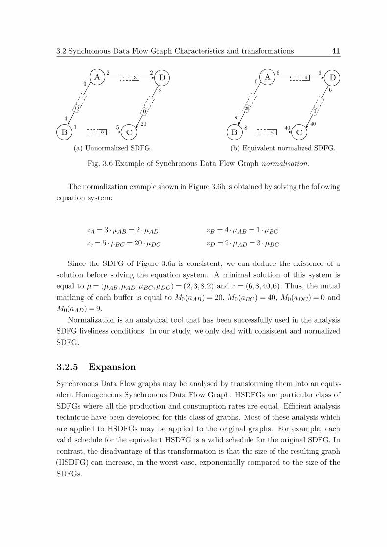
3.2 Synchronous Data Flow Graph Characteristics and transformations 41
(a) Unnormalized SDFG. (b) Equivalent normalized SDFG.
Fig. 3.6 Example of Synchronous Data Flow Graph normalisation.
The normalization example shown in Figure 3.6b is obtained by solving the followingequation system:
zA = 3 ·µAB = 2 ·µAD zB = 4 ·µAB = 1 ·µBC
zc = 5 ·µBC = 20 ·µDC zD = 2 ·µAD = 3 ·µDC
Since the SDFG of Figure 3.6a is consistent, we can deduce the existence of asolution before solving the equation system. A minimal solution of this system isequal to µ = (µAB,µAD,µBC ,µDC) = (2,3,8,2) and z = (6,8,40,6). Thus, the initialmarking of each buffer is equal to M0(aAB) = 20, M0(aBC) = 40, M0(aDC) = 0 andM0(aAD) = 9.
Normalization is an analytical tool that has been successfully used in the analysisSDFG liveliness conditions. In our study, we only deal with consistent and normalizedSDFG.
3.2.5 Expansion
Synchronous Data Flow graphs may be analysed by transforming them into an equiv-alent Homogeneous Synchronous Data Flow Graph. HSDFGs are particular class ofSDFGs where all the production and consumption rates are equal. Efficient analysistechnique have been developed for this class of graphs. Most of these analysis whichare applied to HSDFGs may be applied to the original graphs. For example, eachvalid schedule for the equivalent HSDFG is a valid schedule for the original SDFG. Incontrast, the disadvantage of this transformation is that the size of the resulting graph(HSDFG) can increase, in the worst case, exponentially compared to the size of theSDFGs.
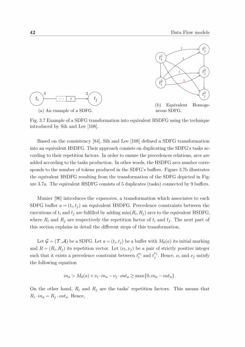
42 Data Flow models
(a) An example of a SDFG.(b) Equivalent Homoge-neous SDFG.
Fig. 3.7 Example of a SDFG transformation into equivalent HSDFG using the techniqueintroduced by Sih and Lee [108].
Based on the consistency [84], Sih and Lee [108] defined a SDFG transformationinto an equivalent HSDFG. Their approach consists on duplicating the SDFG’s tasks ac-cording to their repetition factors. In order to ensure the precedences relations, arcs areadded according to the tasks production. In other words, the HSDFG arcs number corre-sponds to the number of tokens produced in the SDFG’s buffers. Figure 3.7b illustratesthe equivalent HSDFG resulting from the transformation of the SDFG depicted in Fig-ure 3.7a. The equivalent HSDFG consists of 5 duplicates (tasks) connected by 9 buffers.
Munier [96] introduces the expansion, a transformation which associates to eachSDFG buffer a = (ti, tj) an equivalent HSDFG. Precedence constraints between theexecutions of ti and tj are fulfilled by adding min(Ri,Rj) arcs to the equivalent HSDFG,where Ri and Rj are respectively the repetition factor of ti and tj . The next part ofthis section explains in detail the different steps of this transformation.
Let G = (T ,A) be a SDFG. Let a = (ti, tj) be a buffer with M0(a) its initial markingand R = (Ri,Rj) its repetition vector. Let (νi,νj) be a pair of strictly positive integersuch that it exists a precedence constraint between tνi
i and tνj
j . Hence, νi and νj satisfythe following equation
ina > M0(a)+νi · ina−νj ·outa ≥max0, ina−outa.
On the other hand, Ri and Rj are the tasks’ repetition factors. This means thatRi · ina = Rj ·outa. Hence,

3.2 Synchronous Data Flow Graph Characteristics and transformations 43
ina > M0(a)+(νi +Ri) · ina− (νj +Rj) ·outa ≥max0, ina−outa.
This inequalities implies that there is an infinite set of precedence constraints whichare repeated every iteration. An iteration means a phase in which tasks ti and tj areexecuted respectively Ri and Rj times.
The underlying idea of the expansion, is to represent the infinite set of precedenceconstraints induced by the buffer and its initial marking using a finite repetitivestructure, i.e a pattern. This transformation is composed of three steps:
1. Each task ti is replaced by Ri (task repetition factor) tasks denoted by t1i , . . . , tRi
i .
such that for any k ∈ 1, . . . ,Ri and α > 0, the αth execution of tki corresponds
to the ((α−1) ·Ri +k)th execution of ti. Tasks t1i , . . . , tRi
i are called duplicatesof ti.
2. For successive executions of each task, a buffer ak = (tkii , tki+1
i ) is added forki ∈ 1, . . . ,Ri−1 with M0(ak) = 0. In addition, aRi
= (tRii , t1
i ) is added withM0(aRi
) = 1.
3. Arcs are added between tνii and t
νj
j in the following cases:
• If ina > outa, Ri arcs are added between the executions of ti and tj . Theexecutions indexes are computed as follows:
∀νi ∈ 1, . . . ,Ri, νj = ⌊M0(a)+ ina · (νi−1)outa
⌋+1
• If ina ≤ outa, Rj arcs are added between the executions of ti and tj . Theexecutions indexes are computed as follows:
∀νj ∈ 1, . . . ,Rj, νi = ⌈outa ·νj−M0(a)ina
⌉ with νj >M0(a)outa
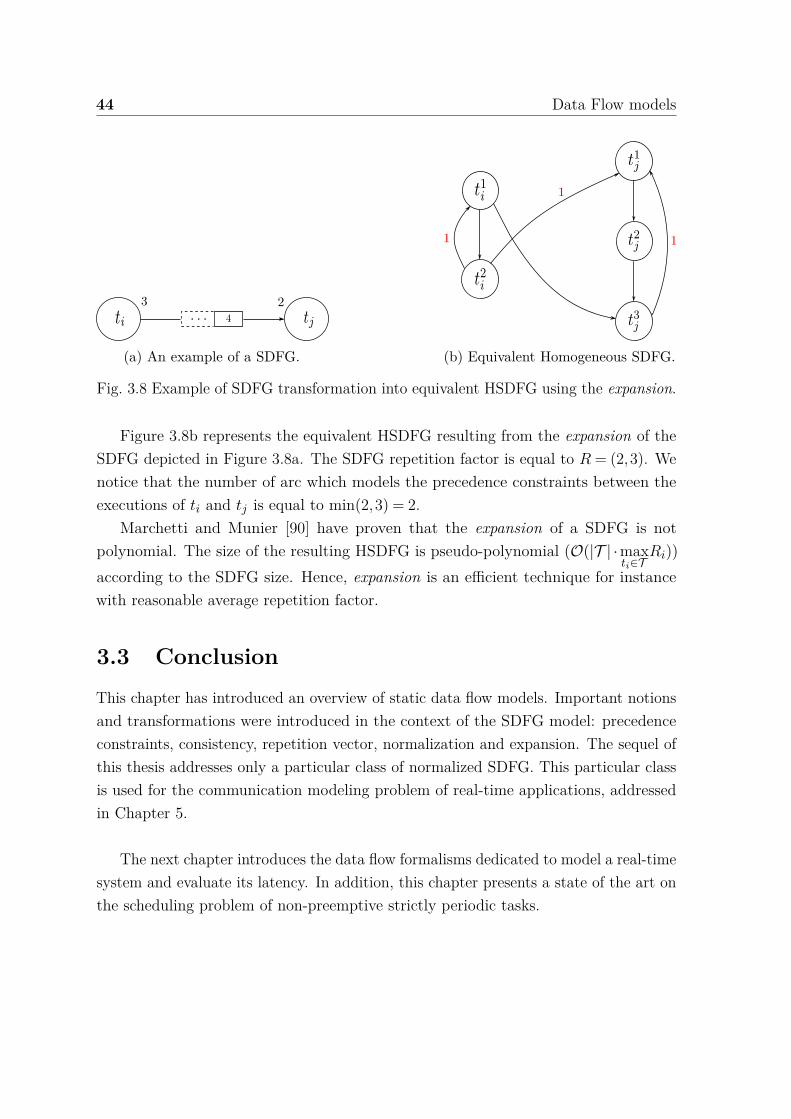
44 Data Flow models
(a) An example of a SDFG. (b) Equivalent Homogeneous SDFG.
Fig. 3.8 Example of SDFG transformation into equivalent HSDFG using the expansion.
Figure 3.8b represents the equivalent HSDFG resulting from the expansion of theSDFG depicted in Figure 3.8a. The SDFG repetition factor is equal to R = (2,3). Wenotice that the number of arc which models the precedence constraints between theexecutions of ti and tj is equal to min(2,3) = 2.
Marchetti and Munier [90] have proven that the expansion of a SDFG is notpolynomial. The size of the resulting HSDFG is pseudo-polynomial (O(|T | ·max
ti∈TRi))
according to the SDFG size. Hence, expansion is an efficient technique for instancewith reasonable average repetition factor.
3.3 ConclusionThis chapter has introduced an overview of static data flow models. Important notionsand transformations were introduced in the context of the SDFG model: precedenceconstraints, consistency, repetition vector, normalization and expansion. The sequel ofthis thesis addresses only a particular class of normalized SDFG. This particular classis used for the communication modeling problem of real-time applications, addressedin Chapter 5.
The next chapter introduces the data flow formalisms dedicated to model a real-timesystem and evaluate its latency. In addition, this chapter presents a state of the art onthe scheduling problem of non-preemptive strictly periodic tasks.
Chapter 4
State of art
Modeling stage is essential for designing real-time systems. This procedure provides anoperational representation of the system. Modeling an application using static dataflow graph provides additional informations related to its execution. Thus, it is possibleto evaluate accurately the system performances. On the other hand, these applicationsmust be (properly) scheduled in order to be executed on a given platform. Schedulersmust take into account several type of constraints such as resource and communicationconstraints.
This chapter gives an overview on the state of the art related to this thesis. Theremainder of this chapter is organized as follows. Section 4.1 positions our study withrespect to the state of the art for modeling real-time systems and evaluating theirlatencies using data flow formalisms. Section 4.2 compares our approach with someexisting non-preemptive strictly periodic scheduling approaches. Conclusion is given inSection 4.3.
4.1 Modeling real time systems using data flow for-malisms
Critical real-time applications are becoming increasingly complex. These applicationsare subject to temporal and data constraints. They require a reliable and predictableimplementation, since a mismatch during the system lifetime can be catastrophic.Therefore, a model is required to represent (in a deterministic way) the communi-cations between the several parts of a real-time application. This section representsseveral studies that have been investigated to study real-time systems using data flowformalisms.
46 State of art
Cyclo-Static Data Flow
In [5, 6, 86], the authors consider acyclic CSDFG applications with a single input.They provide an analytical framework for extracting the timing parameters for theCSDFG actors. They compute the periodic tasks parameters using an estimation ofthe worst-case execution time. They also assume that each read and write has constantexecution time. Each actor of CSDFG were scheduled as an implicit periodic taskwhere its deadline is equal to its period. In our approach, we modelled cyclic andacyclic multi-periodic systems with single/multiple input. Moreover, periodic tasksadmit deadlines which are not necessarily equal to their periods.
Affine Data Flow graph
Bouakaz et al. [20] propose an extension of the CSDFG model called Affine DataFlow graph (ADF in short). This latter is a time-triggered data flow model thatexplicitly represents each task execution during a complete iteration of the graph.Each task is associated with an activation clock and executed at each clock tick. Anycouple clock of ticks in the network can be related by an affine function. Precedenceconstraints between the tasks’ executions are respected since the affine functions ensurethe correct order of clock ticks execution. In this context, the authors proposed ananalysis framework to schedule the actors of the ADF graph as periodic tasks. However,modeling the execution behaviour using the clock ticks and the affine functions delaysthe process of finding a feasible schedule. In fact, representing the execution behaviourwith clock ticks implicitly transforms the ADF into an equivalent HSDFG. In contrast,our approach modeled the communication within a multi-periodic system with a graphwhose size is equal to the number of the system tasks.
Homogeneous Synchronous Data Flow Graph
In [60, 59], Hausmans et al. have presented a temporal analysis for fixed-priorityscheduling. They considered that data flow applications are modelled as cyclic HS-DFG/SDFGs. They compute an upper bound on the worst-case response time ofeach actor. They assume that the data flow graphs have a strictly periodic sourcewhile considering that the other actors have a data-driven operational semantics. Tasktiming properties were extracted based on its interference with the set of higher pri-ority tasks executed on the same platform. This means that the computation of thetiming parameters depends on the set of applications executed on the same platform.Their approaches differ in how to compute that interference. They used a period and

4.1 Modeling real time systems using data flow formalisms 47
jitter characterization [60](difference between best-case and worst-case offsets), anenabling rate characterization [59] (describing for each time interval the minimum andmaximum number of possible task enabling). Unlike their approach, we modeled thecommunications within a multi-rate system independently of the scheduling strategyor the other applications executed on the same platform.
In [2], Ali et al. proposed an algorithm for extracting the real-time propertiesof data flow applications. They extract timing parameters (such as offsets, periodsand deadlines) of data flow applications with timing constraints (such as throughputand latency). Their approach converts each actor into a periodic arbitrary-deadlinetasks. However, their method can only be applied on data flow applications modeledas HSDFGs which are less expressive than SDFGs. In addition, transforming a SDFGinto an equivalent HSDFG requires the use of an unfolding process that duplicateseach actor potentially an exponential number of times.
Synchronous Data Flow Graph
Recently, Singh et al. [109] extended the SDFG model in order to incorporate real-timeproperties. They associate to each actor a worst-case execution time. Moreover, theyspecify to each SDFG a single input and output actors with repetition factors equal to 1.Each SDFG was also characterized by a period and a relative deadline parameters. Inorder to schedule the SDFG upon preemptive uniprocessor, they developed an algorithmconverting any SDFG task into a collection of equivalent 3-parameter sporadic tasksτi = (Ci,Di,Ti) [94, 10]. These latter have the worst-case computational requirementexactly equal to the worst-case computational requirement of the SDFG task. In thisthesis, we limit our study to periodic tasks. However, we consider that the real-timetasks can admit release dates. In addition, we modeled the communications, within amulti-periodic system using a particular class of SDFGs, without increasing the numberof the system tasks.
4.1.1 Latency evaluation using data flow model
Other authors have modeled real-time applications using data flow graphs in order tocompute their latency.
48 State of art
Processing Graphs Methods
Goddard [48] modeled a real-time data flow application using Processing GraphsMethods (PGM in short). In PGM, a system is expressed as directed graph wherenodes correspond to processing functions and edges correspond to FIFO queues. Real-time requirements were verified using the Rate Based Execution (RBE in short) model.A RBE task t is specified by four parameters (x,y,d,e). The couple (x,y) representsthe rate execution where x is the number of executions during the interval y. A task isalso specified by its deadline d and its execution time e. The latency was measuredas function of the source period. It was bounded according to the sum of the tasksexecution times and the sink deadline. In our approach, the tasks periods are directlyextracted from the real-time application. Hence, latency is computed according to theparameters of each couple of periodic communicating tasks which is more expressive interms of the system’s communications.
Homogeneous Synchronous Data Flow Graph
Moreira et al. [95] studied real-time scheduling of data flow programs using Homo-geneous SDFG. In this latter, the consumption and production rates are equal to1. Some tasks were added to the equivalent HSDFG in order to enforce the strictlyperiodic behaviour within a self-timed implementation. They defined latency as thetime interval between two events. Latency between periodic tasks were computed onlyif their repetition factors are equal. However, our communication model allows toevaluate the latency between periodic tasks having different repetition factors. DespiteSDFG is known to be convertible into HSDFG, Marcheti and Munier [90] have proventhat this conversion is not polynomial.
In [36, 35], authors proposed an analytical framework for computing the periodictasks’ parameters for an application modeled as acyclic CSDFG, so that the tasksare scheduled in a strictly periodic manner. Accordingly, they compute the latencybetween the executions of two dependent tasks . Moreover, they defined the systemlatency as an iteration during which each task is executed according to its repetitionfactor.
4.1.2 Main difference
Existing techniques [48, 95, 5, 20, 60, 2, 109], transform each actor in a given data flowinto (independent/dependent) real-time task(s). Tasks’ parameters are specified so thatthe data flow temporal behavior is correctly reflected. Accordingly, scheduling data

4.2 Scheduling strict periodic non-preemptive tasks 49
flow graph is equivalent to schedule the set of real-time tasks. This can be done usingexisting analysis frameworks developed for real-time systems. In contrast, our approachconsists in modeling communications within multi-periodic systems. We assume thatthe periodic tasks parameters and their communication scheme are user-provided.We describe how inter-task dependencies (at the job level) can be modeled using aparticular class of SDFG [73]. Consequently, scheduling a multi-periodic system isequivalent to schedule a SDFG using techniques (methods) that have be developedwithin the SDFG community.
4.2 Scheduling strict periodic non-preemptive tasksA real-time task is considered schedulable if its worst-case response time under a givenscheduling algorithm is less than or equal to its deadline. Consequently, a set of tasksis schedulable under a given scheduling algorithm if all of its tasks are schedulable.Real-time scheduling theory yields several schedulability conditions in order to verifywhether a set of tasks is schedulable under a given scheduling algorithm. Given asystem and scheduling algorithm, a schedulability condition is termed sufficient, ifall of the system tasks that are deemed schedulable according to the condition arein fact schedulable [33]. Similarly, a schedulability test is termed necessary, if all ofthe system tasks that are deemed unschedulable according to the condition are in factunschedulable [33]. Moreover, a schedulability condition that is both sufficient andnecessary is an exact schedulability condition.
In this section, we present some studies from the literature concerned with schedulingof applications modeled as real-time periodic tasks. More precisely, we emphasis onthe scheduling problem for non-preemptive strictly periodic tasks. In this case, thesuccessive executions of each task admit periodic starting dates that are separated bythe task period.
4.2.1 Preemptive uniprocessor schedulability analysis
In this subsection, we present two well-known scheduling algorithms and their schedu-lability test upon preemptive uniprocessor. These algorithms are Rate Monotonic (RMin short) and Early Deadline First (EDF in short).

50 State of art
Rate Monotonic
The RM algorithm [85] is a preemptive scheduling with static priorities that areassigned to a set of independent periodic tasks according to their rates (periods).Higher execution priority is given to the task with the smaller period. The RMalgorithm is considered as a fixed-priority algorithm, since the tasks periods areconstant. The sufficient schedulability condition of an implicit-deadline periodic taskset on uniprocessor using RM algorithm can be verified through the processor utilization,as follows:
Theorem 4.2.1 A set of independent periodic tasks T = t1, . . . , tn with implicit-deadlines is schedulable using RM if
∑ti∈T
ui ≤ n(21n −1).
Given an implicit-deadline periodic task set, RM is optimal among all fixed-priorityalgorithms. In other words, if a fixed-priority algorithm can schedule a set of implicit-deadline tasks, RM does it as well. However, RM is not optimal on uniprocessor fornon-preemptive periodic tasks.
Early Deadline First
EDF algorithm [85] is a scheduling algorithm that schedules the executions of thetasks according to their absolute deadlines. Higher execution priority is given to taskexecution with earlier deadline. EDF algorithm is optimal for independent implicit-deadline periodic task set on preemptive uniprocessor. The schedulability conditioncan be verified through the processor utilization, as follows:
Theorem 4.2.2 A set of independent tasks T = t1, . . . , tn with implicit-deadlines isschedulable using EDF if and only if
∑ti∈T
ui ≤ 1.
Baruah et al. [11] provide a sufficient and necessary condition for scheduling aconstrained-deadline periodic tasks using EDF on uniprocessor. However, this schedu-lability test is very time consuming, since it is know to be co-NP-complete in strongsense.
In this thesis, we focus our study on scheduling applications modeled as non-preemptive strictly periodic tasks.
4.2 Scheduling strict periodic non-preemptive tasks 51
4.2.2 Scheduling non-preemptive strictly periodic systems
In real-time systems, scheduling of preemptive periodic tasks have been extensivelystudied. Many uniprocessor schedulability conditions have been developed for severalpreemptive algorithms such as RM and EDF [85]. Goossens et al. [49] studied theproblem of scheduling offset free systems. They propose a schedulability condition onmulti-core platform using EDF algorithm. Their approach has polynomial time com-plexity. Unfortunately, George et al. [45] proved that the schedulability conditions inpreemptive scheduling become, at best, necessary conditions in the non-preemptive case.
Non-preemptive scheduling problems must be studied since their resolution may offeradvantages in term of schedulability. Several studies considered preemptive schedulingconditions in order to obtain the conditions for the non-preemptive versions. Takinginto consideration the extra interference time caused by non-preemption, Baruah [9]followed the similar method in [49] and provided a sufficient schedulability conditionfor non-preemptive periodic tasks. Based on the problem windows analysis [8], Guanet al. [55] studied the problem of global non-preemptive fixed priority scheduling. Inour approach, we consider a set of non-preemptive tasks.
Furthermore, other studies focused on non-preemptive scheduling. Jeffay et al.[65] showed that non-preemptive scheduling of real-time tasks is an NP-hard problem.They also derived a necessary and sufficient condition for the non-preemptive EarliestDeadline First scheduling algorithm (npEDF in short) when tasks are periodic witharbitrary offsets. Recently, Nasri et al. [97] showed that the latter condition is verypessimistic in the special case of harmonic tasks. They also studied the non-preemptiveRate Monotonic (npRM in short) for the same type of tasks and derived a sufficientcondition of schedulability for both npRM and npEDF. The same authors [98] proposeda scheduling algorithm called “Precausious-RM” or “P-RM”. It is an online algorithmfor scheduling periodic non-preemptive harmonic task set, with linear complexity. Arelaxed algorithm derived from P-RM is also proposed thereafter, called “Lazy P-RM”.This algorithm improves the performance of P-RM when task execution times are short.In these works [65, 97, 98], non-preemptive periodic tasks were studied. However,in this thesis, we consider strictly periodic constraints. In the sequel, we presentsome studies from the literature concerned with scheduling of applications modeled asnon-preemptive strictly periodic tasks.

52 State of art
Scheduling independent non-preemptive strictly periodic tasks
A more particular scheduling problem is the one with non-preemptive strictly periodictasks. The non-preemptive scheduling problem is known to be NP-hard computationalcomplexity [65]. Adding the strict periodicity constraint increases the problem com-plexity. Korst et al. [80] were the first to study the problem of scheduling a set ofnon-preemptive strictly periodic tasks. Their work was motivated by real-time videosignal processing. The authors considered this problem on a minimum number ofprocessors [79]. They showed that the problem is NP-complete in the strong sense, evenin the case of a single processor, but that it is solvable in polynomial time if the periodsand execution times are divisible. Thus, they proposed an approximation algorithmbased on assigning tasks to processors according to some priority rule. Besides, theyproposed a necessary and sufficient condition for the schedulability of two strictlyperiodic tasks. Later, Kermia et al [70] proposed a sufficient schedulability conditionthat generalizes the previous condition for a set of tasks. They imposed that the sumof the tasks execution times is less or equal to the greatest common divisors (GCDs)of task periods. In [92], Marouf and Sorel proved that this sufficient condition is veryrestrictive (pessimistic). They also gave a schedulability condition for implicit-deadlinestrictly periodic tasks and proposed an heuristic based on this condition. In contrast,our approach is not restricted to implicit-deadline tasks.
Eisenbrand et al. [37] considered the problem of scheduling non-preemptive strictlyperiodic tasks in order to minimize the number of processors. They studied taskswith harmonic periods, i.e., every period divides all other periods of greater value.In this case, they showed that there exists a 2-approximation for the minimizationproblem and that this result is tight. The same authors added additional constraints tothe same problem with harmonic tasks and proposed an Integer Linear Programming(ILP) formulation and primal heuristics [38]. Marouf and Sorel [93] proposed a similarwork and gave a scheduling heuristic. This latter is based on the constraint that theperiod of a candidate task has a multiple relationship with the task periods alreadyscheduled. However, this thesis addresses a more challenging problem which is dealingwith harmonic and non-harmonic periods.
Al-Sheikh et al. [1] used the Mixed Integer Linear Program (MILP) formulation inorder to establish an exact framework for non-preemptive strictly periodic schedulingproblem in Integrated Modular Avionics (IMA) platform. Afterwards, they proposeda best-response algorithm based on game theory [44]. This algorithm consists in

4.2 Scheduling strict periodic non-preemptive tasks 53
computing the largest possible change for all task execution times. Accordingly, theydetermined whether all tasks are schedulable upon a limited number of processors.Pira and Artigues [102] improved the best-response algorithm using a propagationmechanism and local optimizations. However, in our study we consider that the userprovides all the tasks parameters.
Chen et al. [26] represented a strictly periodic task by its eigentask, i.e., a task thathas the same period as the original task and an execution time equal to one. Assumingthat a set of tasks is already scheduled on a given processor, they proposed a sufficientcondition to determine whether a new task is schedulable on the same processor. Basedon this condition, they developed a task assignment algorithm to allocate the tasks andcompute an upper bound of the number of required processors . Afterwards, Chen etal. [25] adopted the idea of eigentask. They used a more efficient method to calculatethe valid scheduling slots of an eigentask. In addition, they developed an heuristic thatassigned the tasks to required processors. In their approach, the tasks priorities werenot considered during the assignment step.
As mentioned previously, several studies [92, 37, 38, 93, 1, 102, 26, 25] investigatedthe scheduling problem of independent non-preemptive strictly periodic tasks. Theseapproaches considered uniprocessor/multiprocessor scheduling problem. Tasks wereassigned to the same processor either with harmonic or non-harmonic periods. However,none of these approaches considered the scheduling of dependent tasks set. In otherwords, these approaches do not take into account the communication constraintsbetween the tasks executions. In this thesis, we tackle the mono-processor schedulingproblem of strictly periodic tasks subject to communication constraints.
Scheduling dependent non-preemptive strictly periodic tasks
Other authors considered the scheduling problem of dependent non-preemptive strictlyperiodic tasks, taking into consideration data exchange (at the job level). Dependencybetween the tasks executions were modeled as precedence constraints.
Cucu and Sorel [30] considered the problem of multiprocessor scheduling of strictlyperiodic systems with communication requirements. They used a graph-based modelto specify the precedence between the tasks executions through acyclic graphs [29]. Intheir approach, a precedence constraint between a pair of tasks (ti, tj) imposes thatthe period of ti must be less or equal to that of its successor tj . Communication (data
54 State of art
transfer) between tasks is only restricted to tasks that are executed at the same rate.In order to solve the scheduling problem, they proposed an heuristic and compared itsperformance to an exact “Branch & Bound” algorithm [82].
Based on the previous work, Kermia et al. [70] proposed a greedy heuristic forallocating and scheduling non-preemptive dependent strictly periodic systems ontomulti-core platform. Their approach is composed of several algorithms. Assuminga scheduling frame whose length is equal to the system hyper-period, each task wasduplicated (hp
T ) times, where T is a task period and hp is the hyper-period. Arcs wereadded between duplicates in order to represent precedence constraints between thetasks executions. Duplicates were classified and assigned to processors according totheir periods (in an increasing order). Their assignment favours mapping duplicateswhose periods are equal or multiples on the same processor. Finally, an extension ofthe SynDEx heuristic [54] was applied onto the unrolled graph instead of the originalone. Afterwards, the same authors [71] improved their assignment algorithm using amixed sort which takes into account both the tasks periods (in an increasing order)and a priority level. In addition, data transfer can only be occurred between two taskshaving the same or multiple periods. The heuristic performance was compared to anoptimal “Branch and Cut” algorithm [88].
Contrary to the previous works [30, 70, 71], in this thesis, we limit our studyto uniprocessor scheduling problem of strictly priodic communicating tasks. In ourapproach, tasks admit release dates and relative deadlines (user-provided). Communica-tion scheme between the tasks execution is build according to these parameters (releasedates and relative deadlines). Consequently, our framework allows communicationbetween tasks with arbitrary periods. In order to solve this scheduling, we propose anexact (optimal) algorithm and three heuristics. These methods are able to schedulecyclic and acyclic systems on a single processor. Furthermore, our heuristics do notincrease the number of tasks in order to schedule them on the same processor. In otherwords, we do not convert our original graph into an equivalent graph that models thecommunications between the tasks executions. This transformation is not polynomialand can be very time consuming [90]. Finally, tasks with non-harmonic periods can beassigned to the same processor.

4.3 Conclusion 55
4.3 ConclusionIn recent years, several models have been developed to study data flow graphs froma real-time point of view. This problem has been studied by researchers from both(real time and data flow) communities. Conversely to the approaches proposed in theliterature, our approach consists in studying communications within a multi-periodicsystem from a data flow point of view.
On the other hand, scheduling applications modeled as non-preemtive strictlyperiodic tasks is very challenging, since this problem is known to be NP-complete instrong sense. Several approaches introduced in the literature considered the schedulingproblem of an independent strictly periodic set of tasks. Unfortunately, only fewauthors tackled this scheduling problem with communication (precedence) constraintsbetween the tasks executions. In order to meet this challenge, we propose in chapter 6an optimal algorithm and three heuristics that solve the scheduling problem of strictlyperiodic systems subject to communication constraints.
The following chapter presents the first contribution of this thesis. This contributionconsists in modeling the communications within a multi-periodic systems and evaluatingtheir (worst-case) latencies using data flow formalisms.


Chapter 5
Real Time Synchronous Data FlowGraph (RTSDFG)
Nowadays, real-time applications are invading our daily life. These systems are highlycritical, as a mismatch during the system lifetime can be catastrophic. In this context,one of the major challenges faced by academic and industrial environments is the effi-cient use of powerful and complex material, to provide optimal performance (producingthe right outputs for given inputs) and meet the time constraints (producing outputsat the right time). These systems are usually multi-periodic, since their componentscommunicate with each other at different rates (this is mainly due to their physicalcharacteristic). For this reason, a deep analysis of communications between tasks of amulti-periodic system is required. Moreover, the estimation of parameters in a staticmanner, such as evaluating the latency between the system input and its correspondingoutcome, is an important practical issue.
In this chapter, we seek to model the communications within multi-periodic systemsusing SDGF formalisms. Section 5.1 is dedicated to define the “Real-Time SynchronousData Flow Graph”. This latter describes the communication model within a multi-periodic system. Computing the latency between two periodic communicating tasks isdeveloped in section 5.2. Several methods for evaluating the worst case system latencyare explicitly described in Section 5.3. Experimental results of these methods arerepresented in Chapter 7. Conclusion is stated in Section 5.4.
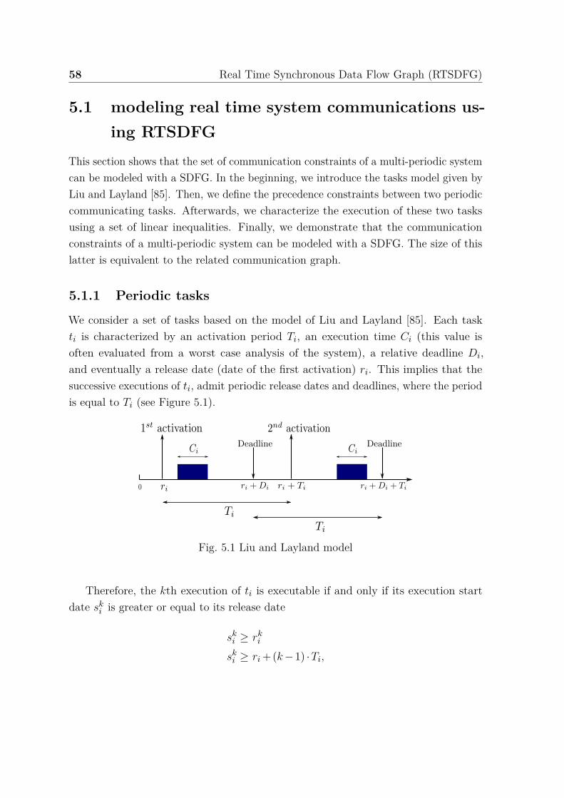
58 Real Time Synchronous Data Flow Graph (RTSDFG)
5.1 modeling real time system communications us-ing RTSDFG
This section shows that the set of communication constraints of a multi-periodic systemcan be modeled with a SDFG. In the beginning, we introduce the tasks model given byLiu and Layland [85]. Then, we define the precedence constraints between two periodiccommunicating tasks. Afterwards, we characterize the execution of these two tasksusing a set of linear inequalities. Finally, we demonstrate that the communicationconstraints of a multi-periodic system can be modeled with a SDFG. The size of thislatter is equivalent to the related communication graph.
5.1.1 Periodic tasks
We consider a set of tasks based on the model of Liu and Layland [85]. Each taskti is characterized by an activation period Ti, an execution time Ci (this value isoften evaluated from a worst case analysis of the system), a relative deadline Di,and eventually a release date (date of the first activation) ri. This implies that thesuccessive executions of ti, admit periodic release dates and deadlines, where the periodis equal to Ti (see Figure 5.1).
Fig. 5.1 Liu and Layland model
Therefore, the kth execution of ti is executable if and only if its execution startdate sk
i is greater or equal to its release date
ski ≥ rk
i
ski ≥ ri +(k−1) ·Ti,
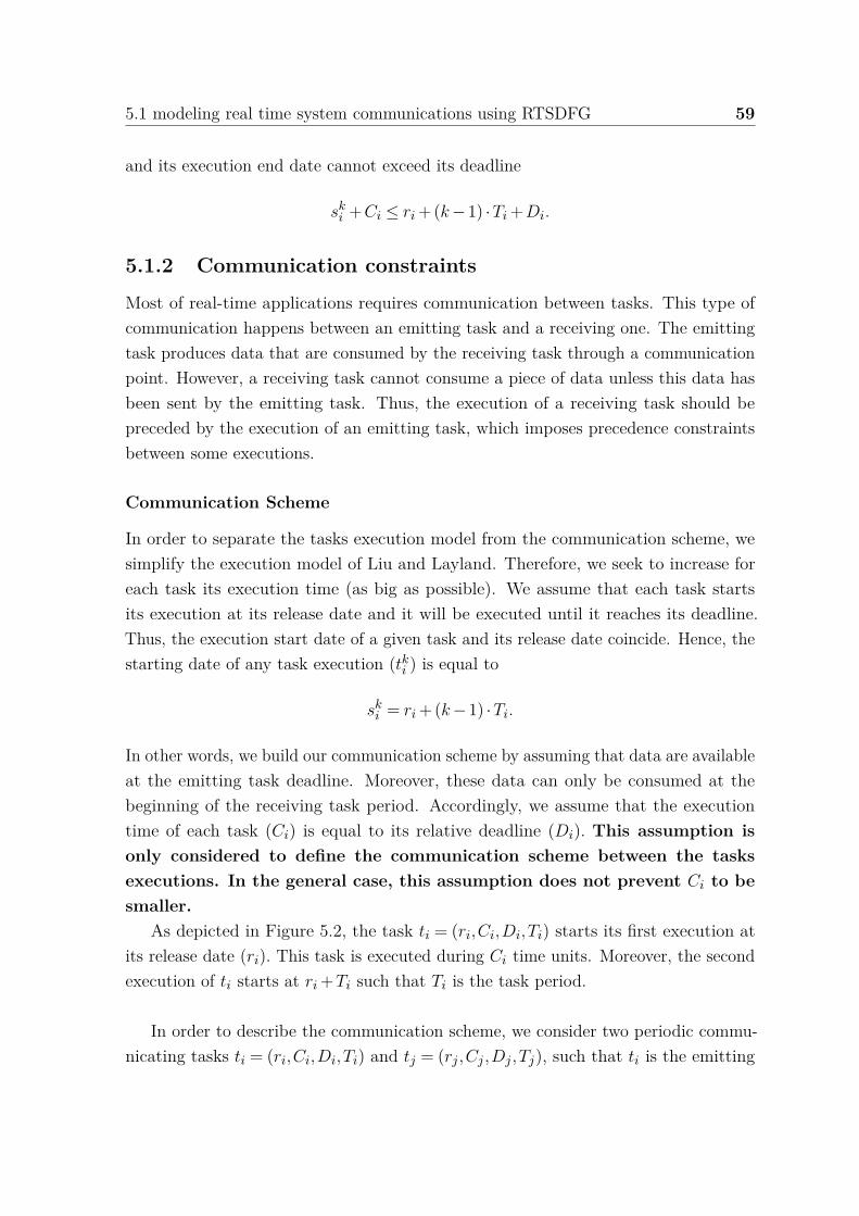
5.1 modeling real time system communications using RTSDFG 59
and its execution end date cannot exceed its deadline
ski +Ci ≤ ri +(k−1) ·Ti +Di.
5.1.2 Communication constraints
Most of real-time applications requires communication between tasks. This type ofcommunication happens between an emitting task and a receiving one. The emittingtask produces data that are consumed by the receiving task through a communicationpoint. However, a receiving task cannot consume a piece of data unless this data hasbeen sent by the emitting task. Thus, the execution of a receiving task should bepreceded by the execution of an emitting task, which imposes precedence constraintsbetween some executions.
Communication Scheme
In order to separate the tasks execution model from the communication scheme, wesimplify the execution model of Liu and Layland. Therefore, we seek to increase foreach task its execution time (as big as possible). We assume that each task startsits execution at its release date and it will be executed until it reaches its deadline.Thus, the execution start date of a given task and its release date coincide. Hence, thestarting date of any task execution (tk
i ) is equal to
ski = ri +(k−1) ·Ti.
In other words, we build our communication scheme by assuming that data are availableat the emitting task deadline. Moreover, these data can only be consumed at thebeginning of the receiving task period. Accordingly, we assume that the executiontime of each task (Ci) is equal to its relative deadline (Di). This assumption isonly considered to define the communication scheme between the tasksexecutions. In the general case, this assumption does not prevent Ci to besmaller.
As depicted in Figure 5.2, the task ti = (ri,Ci,Di,Ti) starts its first execution atits release date (ri). This task is executed during Ci time units. Moreover, the secondexecution of ti starts at ri +Ti such that Ti is the task period.
In order to describe the communication scheme, we consider two periodic commu-nicating tasks ti = (ri,Ci,Di,Ti) and tj = (rj ,Cj ,Dj ,Tj), such that ti is the emitting

60 Real Time Synchronous Data Flow Graph (RTSDFG)
Fig. 5.2 Simplification of Liu and layland’s model
task and tj is the receiving one. Let νi and νj be a pair of strictly positive integers.There exists a precedence constraint between the νith execution of ti and the νjthexecution of tj if and only if the three following conditions are met:
1. The νjth execution of tj cannot begin before the end of the νith execution of ti,
thus
sνii +Ci ≤ s
νj
j
ri +(νi−1) ·Ti +Di ≤ rj +(νj−1) ·Tj (5.1)
2. There is no precedence constraint between the (νi +1)th execution of ti and theνjth execution of tj , since the νjth execution of tj starts before the end of the(νi +1)th execution of ti, hence
sνi+1i +Ci > s
νj
j
ri +νi ·Ti +Di > rj +(νj−1) ·Tj . (5.2)
3. There is no precedence constraint between the νith execution of ti and the(νj−1)th execution of tj , since the (νj−1)th execution of tj begins before theend of νith execution of ti, so
sνii +Ci > s
νj−1j
ri +(νi−1) ·Ti +Di > rj +(νj−2) ·Tj . (5.3)
Example 5.1.1 Let us consider ti = (ri,Ci,Di,Ti), tj = (rj ,Cj ,Dj ,Tj) two periodiccommunicating tasks. We suppose that Ti = 30, Tj = 40 time units, Ci = Di = 20 timeunits, Cj = Dj = 20 time units, and their release dates are null (ri = rj = 0). Figure5.3 illustrates the precedence constraints between the tasks executions. We notice the

5.1 modeling real time system communications using RTSDFG 61
Fig. 5.3 Example of multi-periodic communication model
existence of a precedence constraint between the first execution of ti and the secondexecution of tj . In fact, equation (5.1) is fulfilled since the second execution of tj didnot start before the end of the first execution of ti. Furthermore, we notice the absenceof precedence constraints between t1
i and t1j on one hand, and between t2
i and t2j on
the other hand. In both cases, the corresponding execution of tj begins before the endof ti execution. This means that equation (5.2) and (5.3) are also fulfilled.
The following lemma draws together the three inequalities mentioned before.
Lemma 5.1.1 Let ti = (ri,Ci,Di,Ti) and tj = (rj ,Cj ,Dj ,Tj) be two periodic commu-nicating tasks, with ti the emitting task and tj the receiving one. Let νi and νj be apair of strictly positive integers. There exists a precedence constraint between the νithexecution of ti and the νjth execution of tj if and only if:
Ti ≥ Tj− rj + ri +Di +νi ·Ti−νj ·Tj > max0,Ti−Tj (5.4)
Proof: Let us consider the inequalities (5.1), (5.2) and (5.3) which define the prece-dence constraints between the different executions of two communicating tasks. Bysubstituting Tj− rj + ri +Di with M, we obtain:
1. Condition 1 is equivalent to:
M+νi ·Ti−νj ·Tj ≤ Ti,
2. Condition 2 is equivalent to:
M+νi ·Ti−νj ·Tj > 0,

62 Real Time Synchronous Data Flow Graph (RTSDFG)
3. Condition 3 is equivalent to:
M+νi ·Ti−νj ·Tj > Ti−Tj .
By combining the three inequalities, we obtain
Ti ≥M+νi ·Ti−νj ·Tj > max0,Ti−Tj .
Let us Consider the communication scheme illustrated in Figure 5.3. Equation (5.4)can be written according to the executions indexes (νi and νj):
30≥ 40+20+30 ·νi−40 ·νj > 0
We verify this inequality for the couples (νi,νj) = (1,2) and (3,3) , which correspondsto the established precedence constraints between t1
i and t2j and between t3
i and t3j .
5.1.3 From real time system to RTSDFG model
Based on the communication rules presented in the previous subsection, we provein this subsection that the set of communication constraints between two periodiccommunicating tasks can be modeled using a SDFG buffer. The buffer production andconsumption rates correspond to the tasks periods and its initial marking is computedwith a close formula according to the tasks parameters. Accordingly, we deduce thatcommunication constraints of a multi-periodic system can be modeled with a particularSDFG. The size of the latter is equal to the system communication graph size.
We note gcda the common period of two communicating tasks ti and tj . It is equalto the greatest common divider of tasks periods, gcda = gcd(Ti,Tj). We assume forwhat follows, that all the tasks parameters are integers.
Theorem 5.1.1 Let ti = (ri,Ci,Di,Ti) and tj = (rj ,Cj ,Dj ,Tj) be two periodic taskssuch that ti communicates with tj. The set of communication constraints between theexecutions of ti and tj can be modeled by a buffer a = (ti, tj) with zi = Ti, zj = Tj andM0 (a) = Tj +λ−gcda with λ =
⌈ri−rj+Di
gcda
⌉·gcda.
Proof: Let us consider a couple of periodic communicating tasks ti = (ri,Ci,Di,Ti)and tj = (rj ,Cj ,Dj ,Tj) such that ti is the emitting task and tj the receiving one. Let(νi,νj) be a pair of strictly positive integers. We assume that there is a precedence
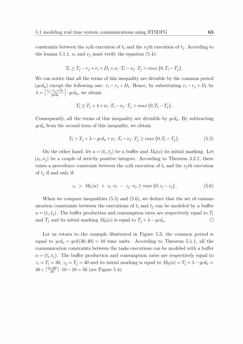
5.1 modeling real time system communications using RTSDFG 63
constraints between the νith execution of ti and the νjth execution of tj . According tothe lemma 5.1.1, νi and νj must verify the equation (5.4):
Ti ≥ Tj− rj + ri +Di +νi ·Ti−νj ·Tj > max0,Ti−Tj .
We can notice that all the terms of this inequality are divisible by the common period(gcda) except the following one: ri− rj + Di. Hence, by substituting ri− rj + Di byλ =
⌈ri−rj+Di
gcda
⌉·gcda, we obtain
Ti ≥ Tj +λ+νi ·Ti−νj ·Tj > max0,Ti−Tj .
Consequently, all the terms of this inequality are divisible by gcda. By subtractinggcda from the second term of this inequality, we obtain
Ti > Tj +λ−gcda +νi ·Ti−νj ·Tj ≥max0,Ti−Tj . (5.5)
On the other hand, let a = (ti, tj) be a buffer and M0(a) its initial marking. Let(νi,νj) be a couple of strictly positive integers. According to Theorem 3.2.1, thereexists a precedence constraint between the νith execution of ti and the νjth executionof tj if and only if:
zi > M0 (a) + zi ·νi − zj ·νj ≥max0, zi− zj . (5.6)
When we compare inequalities (5.5) and (5.6), we deduce that the set of commu-nication constraints between the executions of ti and tj can be modeled by a buffera = (ti, tj) . The buffer production and consumption rates are respectively equal to Ti
and Tj and its initial marking M0(a) is equal to Tj +λ−gcda.
Let us return to the example illustrated in Figure 5.3, the common period isequal to gcda = gcd(30,40) = 10 time units. According to Theorem 5.1.1, all thecommunication constraints between the tasks executions can be modeled with a buffera = (ti, tj). The buffer production and consumption rates are respectively equal tozi = Ti = 30, zj = Tj = 40 and its initial marking is equal to M0(a) = Tj +λ−gcda =40+ ⌈0+20
10 ⌉ ·10−10 = 50 (see Figure 5.4).
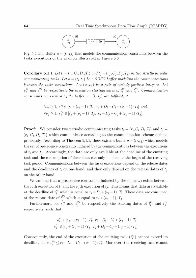
64 Real Time Synchronous Data Flow Graph (RTSDFG)
Fig. 5.4 The Buffer a = (ti, tj) that models the communication constraints between thetasks executions of the example illustrated in Figure 5.3.
Corollary 5.1.1 Let ti = (ri,Ci,Di,Ti) and tj = (rj ,Cj ,Dj ,Tj) be two strictly periodiccommunicating tasks. Let a = (ti, tj) be a SDFG buffer modeling the communicationsbetween the tasks executions. Let (νi,νj) be a pair of strictly positive integers. Letsνi
i and sνj
j be respectively the execution starting dates of tνii and t
νj
j . Communicationconstraints represented by the buffer a = (ti, tj) are fulfilled, if
∀νi ≥ 1, sνii ∈ [ri +(νi−1) ·Ti, ri +Di−Ci +(νi−1) ·Ti] and,
∀νj ≥ 1, sνj
j ∈ [rj +(νj−1) ·Tj , rj +Dj−Cj +(νj−1) ·Tj ].
Proof: We consider two periodic communicating tasks ti = (ri,Ci,Di,Ti) and tj =(rj ,Cj ,Dj ,Tj) which communicate according to the communication scheme definedpreviously. According to Theorem 5.1.1, there exists a buffer a = (ti, tj) which modelsthe set of precedence constraints induced by the communications between the executionsof ti and tj . Accordingly, the data are only available at the deadline of the emittingtask and the consumption of these data can only be done at the begin of the receivingtask period. Communications between the tasks executions depend on the release datesand the deadlines of ti on one hand, and they only depend on the release dates of tj
on the other hand.We assume that a precedence constraint (induced by the buffer a) exists between
the νith execution of ti and the νjth execution of tj . This means that data are availableat the deadline of tνi
i which is equal to ri +Di + (νi−1) ·Ti. These data are consumedat the release date of t
νj
j which is equal to rj +(νj−1) ·Tj .
Furthermore, let sνii and s
νj
j be respectively the starting dates of tνii and t
νj
j
respectively, such that
sνii ∈ [ri +(νi−1) ·Ti, ri +Di−Ci +(νi−1) ·Ti]
sνj
j ∈ [rj +(νj−1) ·Tj , rj +Dj−Cj +(νj−1) ·Tj ]
Consequently, the end of the execution of the emitting task (tνii ) cannot exceed its
deadline, since sνii ≤ ri + Di−Ci + (νi− 1) ·Ti. Moreover, the receiving task cannot
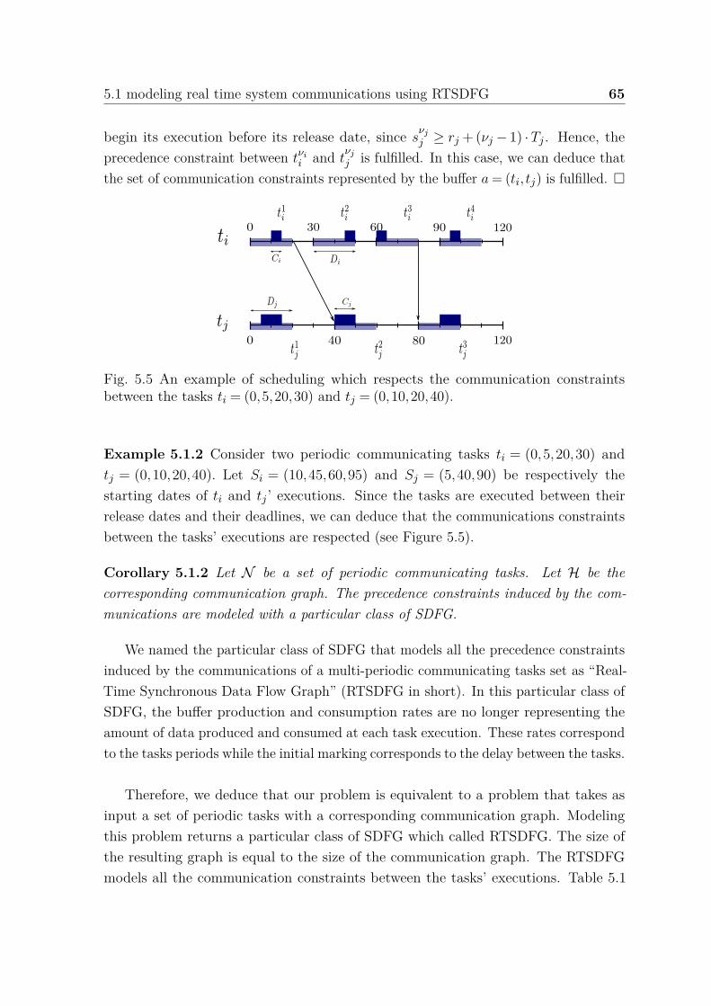
5.1 modeling real time system communications using RTSDFG 65
begin its execution before its release date, since sνj
j ≥ rj + (νj − 1) ·Tj . Hence, theprecedence constraint between tνi
i and tνj
j is fulfilled. In this case, we can deduce thatthe set of communication constraints represented by the buffer a = (ti, tj) is fulfilled.
Fig. 5.5 An example of scheduling which respects the communication constraintsbetween the tasks ti = (0,5,20,30) and tj = (0,10,20,40).
Example 5.1.2 Consider two periodic communicating tasks ti = (0,5,20,30) andtj = (0,10,20,40). Let Si = (10,45,60,95) and Sj = (5,40,90) be respectively thestarting dates of ti and tj ’ executions. Since the tasks are executed between theirrelease dates and their deadlines, we can deduce that the communications constraintsbetween the tasks’ executions are respected (see Figure 5.5).
Corollary 5.1.2 Let N be a set of periodic communicating tasks. Let H be thecorresponding communication graph. The precedence constraints induced by the com-munications are modeled with a particular class of SDFG.
We named the particular class of SDFG that models all the precedence constraintsinduced by the communications of a multi-periodic communicating tasks set as “Real-Time Synchronous Data Flow Graph” (RTSDFG in short). In this particular class ofSDFG, the buffer production and consumption rates are no longer representing theamount of data produced and consumed at each task execution. These rates correspondto the tasks periods while the initial marking corresponds to the delay between the tasks.
Therefore, we deduce that our problem is equivalent to a problem that takes asinput a set of periodic tasks with a corresponding communication graph. Modelingthis problem returns a particular class of SDFG which called RTSDFG. The size ofthe resulting graph is equal to the size of the communication graph. The RTSDFGmodels all the communication constraints between the tasks’ executions. Table 5.1

66 Real Time Synchronous Data Flow Graph (RTSDFG)
presents a set of periodic tasks N = t1, t2, t3. The tasks communication relationshipsE = (t1, t2),(t1, t3),(t2, t1),(t3, t2) are depicted in Figure 5.6. The RTSDFG associatedto this multi-periodic system is depicted in Figure 5.7.
ti ri Ci Di Ti
t1 0 5 20 30t2 20 10 20 40t3 5 5 10 20
Table 5.1 Periodic tasks parameters Fig. 5.6 Communication graph H
Fig. 5.7 The RTSDFG that models the communications between the tasks’ executionsof the multi-periodic system presented in Table 5.1 and Figure 5.6
In the previous parts of this chapter, we proposed a general and intuitive communi-cation model between multi-periodic tasks. Now, the question that needs to be raisedis:
How to compute the latency of a multi-periodic system using a Real-Time Syn-chronous Data Flow Graph?The next part of this chapter answers this question in two steps. First, we computethe latency between two periodic communicating tasks, then we compute the worstcase system latency using several approaches.
5.2 Evaluating latency between two periodic com-municating tasks
In this section, we define the latency between two periodic communicating tasks. Weshow that the latency between the tasks executions is calculated with a closed formula

5.2 Evaluating latency between two periodic communicating tasks 67
according to the tasks parameters. Moreover, we express the maximum and minimumlatency between two communicating tasks with closed formulas. Finally, we prove thatthe minimum and maximum latency can be bounded according to the tasks periods.
In order to evaluate the worst-case system latency, we assume that each task startsits execution at its release date and it will be executed until its deadline. Accordingto this assumption, evaluating the latency between two communicating executions, isequivalent to compute the duration between the data availability and its consumption.
5.2.1 Definitions
Definition 5.2.1 Latency is the time gap between the moment that a stimulationappears and the moment that its reaction begins or ends. Evaluating the latency Lbetween two executions of periodic communicating tasks, is equivalent to compute theduration between the execution end date of the emitting task and the execution startdate of the receiving task (since we assume that each task starts its execution at itsrelease date and ends at its deadline).
Definition 5.2.2 Let ti and tj be a couple of periodic communicating tasks. Weconsider the set E (ti, tj) of couples (νi,νj) ∈ N∗2, such that there exists a precedenceconstraint between tνi
i and tνj
j .
Definition 5.2.3 Let tνii and t
νj
j be a couple of executions with (νi,νj) ∈ E(ti, tj).Hence, t
νj
j cannot start its execution before the end of tνii . We denote by L(tνi
i , tνj
j ) thelatency between the νith execution of ti and the νjth execution of tj. This latency canbe computed as follows:
L(tνii , t
νj
j ) = sνj
j − (sνii +Ci)
= rj +(νj−1) ·Tj− (ri +(νi−1) ·Ti +Di).
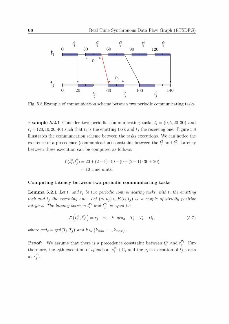
68 Real Time Synchronous Data Flow Graph (RTSDFG)
Fig. 5.8 Example of communication scheme between two periodic communicating tasks.
Example 5.2.1 Consider two periodic communicating tasks ti = (0,5,20,30) andtj = (20,10,20,40) such that ti is the emitting task and tj the receiving one. Figure 5.8illustrates the communication scheme between the tasks executions. We can notice theexistence of a precedence (communication) constraint between the t2
i and t2j . Latency
between these execution can be computed as follows:
L(t2i , t2
j) = 20+(2−1) ·40− (0+(2−1) ·30+20)= 10 time units.
Computing latency between two periodic communicating tasks
Lemma 5.2.1 Let ti and tj be two periodic communicating tasks, with ti the emittingtask and tj the receiving one. Let (νi,νj) ∈ E (ti, tj) be a couple of strictly positiveintegers. The latency between tνi
i and tνj
j is equal to:
L(tνii , t
νj
j
)= rj− ri−k ·gcda−Tj +Ti−Di, (5.7)
where gcda = gcd(Ti,Tj) and k ∈ kmin, . . . ,kmax .
Proof: We assume that there is a precedence constraint between tνii and t
νj
j . Fur-thermore, the νith execution of ti ends at sνi
i +Ci and the νjth execution of tj startsat s
νj
j .

5.2 Evaluating latency between two periodic communicating tasks 69
By assumption, sνii = ri + (νi−1) ·Ti and s
νj
j = rj + (νj−1) ·Tj . Therefore, thelatency between the νith execution of ti and the νjth execution of tj is equal to
L(tνii , t
νj
j
)= s
νj
j − (sνii +Ci)
= rj +(νj−1) ·Tj− ri− (νi−1) ·Ti−Di.
Then, we consider a RTSDFG buffer a = (ti, tj). The buffer production andconsumption rates are respectively equal to Ti and Tj , and its initial marking is equalto M0(a) = Tj + λ− gcda. According to Theorem 5.1.1, the buffer a models all thecommunication constraints between tasks executions. Therefore, Lemma 3.2.1 ofChapter 3 establishes a relation between the indexes of two adjacent tasks connectedby a buffer. According to this lemma, there exists an integer k ∈ kmin, . . . ,kmax suchthat νj = Ti·νi−k·gcda
Tj, with kmin = max0,Ti−Tj−M0(a)
gcdaand kmax = Ti−M0(a)
gcda−1.
Hence, the latency between νith execution of ti and the νjth execution of tj can becomputed as follows:
L(tνii , t
νj
j
)= rj +(νj−1) ·Tj− ri− (νi−1) ·Ti−Di
= rj +(
Ti ·νi−k ·gcda
Tj−1
)·Tj− ri− (νi−1) ·Ti−Di
= rj− ri−k ·gcda−Tj +Ti−Di
Let us consider the communication scheme depicted in Figure 5.8. Let a = (ti, tj)be the RTSDFG buffer that models the communication constraints between the tasksexecutions. The buffer production and consumption rates are respectively equal to 30and 40 and its initial marking is equal to 30. Therefore,
kmin = max0,30−40−3010 =−3,
kmax = 30−3010 −1 =−1.
Hence, we can deduce that the latency between tνii and t
νj
j such that (νi,νj) ∈E(ti, tj),can be computed as follows:

70 Real Time Synchronous Data Flow Graph (RTSDFG)
L(tνii , t
νj
j
)= rj− ri−k ·gcda−Tj +Ti−Di
= 20−0−k ·10−40+30−20=−10 · (k +1),
with k ∈ −3,−2,−1.We apply this result to compute the latency between t2
i and t2j with k =−2,
L(t2i , t2
j) =−10 · (−2+1) = 10 time units.
5.2.2 Maximum latency between two periodic communicat-ing tasks
Definition 5.2.4 We define Lmax(ti, tj) as the maximum latency between the execu-tions of two periodic communicating tasks,
Lmax(ti, tj) = max(νi,νj)∈E(ti,tj)
L(tνii , t
νj
j
).
Theorem 5.2.1 Let ti and tj be two periodic communicating tasks, with ti the emittingtask and tj the receiving one. The maximum latency between executions of these tasksis equal to:
Lmax(ti, tj) = rj− ri−max0,Ti−Tj+λ−gcda +Ti−Di. (5.8)
Proof: We consider two periodic tasks ti and tj . Let (νi,νj) ∈ E (ti, tj) be a coupleof strictly positive integers. According to Lemma 5.2.1, the latency between tνi
i and tνj
j
can be written as follows:
L(νi,νj) (ti, tj) = rj− ri−k ·gcda−Tj +Ti−Di.
In order to evaluate the maximum latency between ti and tj , we substitute k withits minimal value kmin = max0,Ti−Tj−M0(a)
gcda[90]. In this case, we obtain Lmax (ti, tj)
equals to:

5.2 Evaluating latency between two periodic communicating tasks 71
rj− ri−(
max0,Ti−Tj−M0 (a)gcda
)·gcda−Tj +Ti−Di.
Furthermore, M0(a) = Tj +λ−gcda. Hence, Lmax(ti, tj) equals
rj− ri−max0,Ti−Tj+(Tj +λ−gcda)−Tj +Ti−Di.
Finally, we deduce that the maximum latency is equal to
rj− ri−max0,Ti−Tj+λ−gcda +Ti−Di.
In our example, depicted in Figure 5.8, the maximum latency between ti and tj isequal to
Lmax(ti, tj) = rj− ri−max0,Ti−Tj+λ−gcda +Ti−Di
= 20−0−max0,30−40+ ⌈0−20+2010 ⌉ ·10−10+30−20
= 20 time units.
This value corresponds exactly to the duration between the end of t3i and the beginning
of t3j .
Corollary 5.2.1 Let ti and tj be two periodic communicating tasks, with ti the emittingtask and tj the receiving one. the maximum latency value is bounded as follows:
Ti−max0,Ti−Tj−gcda ≤ Lmax(ti, tj) < Ti−max0,Ti−Tj (5.9)
Proof: Let ti and tj two periodic communicating tasks such that ti communicateswith tj . According to Theorem 5.2.1, the maximum latency between the executions ofti and tj can be computed as follows:
Lmax(ti, tj) = rj− ri−max0,Ti−Tj+λ−gcda +Ti−Di,
with λ = ⌈ri−rj+Di
gcda⌉ ·gcda.
On the other hand, λ can be bounded as follows:
ri− rj +Di ≤ λ < ri− rj +Di +gcda

72 Real Time Synchronous Data Flow Graph (RTSDFG)
Furthermore,
0≤ λ− (ri− rj +Di) < gcda,
Ti−max0,Ti−Tj−gcda ≤ λ− (ri− rj +Di)+Ti−max0,Ti−Tj−gcda < Ti−max0,Ti−Tj.
Hence, we can deduce that
Ti−max0,Ti−Tj−gcda ≤ Lmax(ti, tj) < Ti−max0,Ti−Tj
Let us reconsider our example in Figure 5.8. Computing the maximum latencylower and upper bounds between the tasks ti and tj can be done in the following way:
30−max0,30−40−10≤20≤
Lmax(ti, tj)Lmax(ti, tj)
< 30−max0,30−40< 30.
5.2.3 Minimum latency between two periodic communicatingtasks
Definition 5.2.5 We denote by Lmin(ti, tj) the minimum latency between the execu-tions of two communicating tasks,
Lmin(ti, tj) = min(νi,νj)∈E(ti,tj)
L(tνii , t
νj
j ).
Theorem 5.2.2 Let ti and tj be two periodic communicating tasks , with ti the emittingtask and tj the receiving one. The minimum latency between executions of these twotasks is equal to:
Lmin(ti, tj) = rj− ri +λ−Di.
Proof: We consider two periodic tasks ti and tj . Let (νi,νj) ∈ E (ti, tj) a couple ofstrictly positive integers. According to the Lemma 5.2.1, the latency between tνi
i andtνj
j can be written as follows:
L(tνii , t
νj
j
)= rj− ri−k ·gcda−Tj +Ti−Di.

5.2 Evaluating latency between two periodic communicating tasks 73
In order to be able to evaluate the minimum latency between ti and tj , we substitutek with its maximal value kmax = Ti−M0(a)
gcda−1 [90]. In this case, we obtain
Lmin (ti, tj) = rj− ri−kmax ·gcda−Tj +Ti−Di
= rj− ri− (Ti−M0(a)gcda
−1) ·gcda−Tj +Ti−Di
= rj− ri +M0(a)+gcda−Tj−Di.
Furthermore, we have M0 (a) = Tj + λ− gcda. Hence, we deduce that Lmin (ti, tj) isequal to
rj− ri +λ−Di.
Let us consider our communication example depicted in Figure 5.8, the minimumlatency between the tasks executions can be compute as follows:
Lmin(ti, tj) = rj− ri +λ−Di
= 20−0+ ⌈0−20+2010 ⌉ ·10−20
= 0 time units.
This value corresponds exactly to the duration between the end the first execution ofti and the begging of the first execution of tj .
Corollary 5.2.2 Let ti and tj be two periodic communicating tasks, with ti the emittingtask and tj the receiving one. the minimum latency value can be bounded as follows:
0≤ Lmin(ti, tj) < gcda (5.10)
Proof: Let ti and tj two periodic communicating tasks such that ti communicateswith tj . According to the Theorem 5.2.2, the minimum latency between tasks executionscan be computed as follows:
Lmin(ti, tj) = rj− ri +λ−Di,
with λ = ⌈ri−rj+Di
gcda⌉ ·gcda.
On the other hand, λ can be bounded as follows:
ri− rj +Di ≤ λ < ri− rj +Di +gcda.

74 Real Time Synchronous Data Flow Graph (RTSDFG)
Hence, we can deduce that
0≤ Lmin(ti, tj) < gcda.
We apply this result on our example depicted in figure 5.8,
0≤ Lmin(ti, tj) < 10.
5.3 Evaluating the worst-case system latencyThis section presents methods for latency computation of a given system. First, wedefine the worst-case system latency. Then, we present an exact method, that usesall the precedence relationships between tasks’ executions, to compute the latencyvalue. Finally, we propose two algorithms that calculate the system latency upperand lower bounds. These algorithms transform the RTSDFG into an equivalent graphhaving the same size of the RTSDFG. In this graph, the weight of each arc connectingtwo adjacent nodes corresponds to the time required to transfer the data between theperiodic tasks. In order to evaluate the worst-case latency of a multi-periodic system,we limit our study in this thesis to live, consistent and connected acyclic RTSDFGs.Moreover, we compute the system latency using a linear algorithm for computing thelongest path length in a directed acyclic graph.
5.3.1 Definition
Definition 5.3.1 Latency is the delay between the stimulation and response. In otherwords, entire system latency is a time gap between the system input and the connectedoutcome. In our study, we define the worst-case system latency as the longest time gapbetween the system input task executions and the output ones.
As we mentioned before, in order to evaluate the worst-case system latency, weassume that each task of the system starts its execution at its release date and ends atits deadline.

5.3 Evaluating the worst-case system latency 75
Fig. 5.9 Path pth = t1, t2, t3 which corresponds to the communication graph of threeperiodic tasks.
0 30 60 90 120
0 12040 80
0 12040 8020 60 100
150 180 210 240
240160 200
240160 200140 180 220
Fig. 5.10 Communication and execution model of the path pth = t1, t2, t3 depicted inFigure 5.9.
Example 5.3.1 Let t1 = (0,10,20,30), t2 = (0,5,10,20) and t3 = (0,10,20,40) be threeperiodic communicating tasks. Figure 5.9 represents the tasks communication graph.Figure 5.10 illustrates all the communications constraints between the tasks executionsof the path pth = t1, t2, t3. We consider t1 as the system input and t3 the system output.According to our communication model, the data produced by the first execution oft1 is consumed by the second execution of t2, which in turn produces data that isconsumed by the second execution of t3. We summarize all communications constraintsbetween the input and the output tasks’ executions as follows: pth1 = ⟨t1
1→ t22→ t2
3⟩,pth2 = ⟨t2
1→ t42→ t3
3⟩ and pth3 = ⟨t31→ t5
2→ t62→ t4
3⟩. The time required to cover theseexecutions paths is respectively equal to 60,70 and 80 time units. This communicationsand executions pattern is repeated infinitely. Hence, we can deduce that the systemworst-case latency is equal to max60,70,80= 80 time units. This value correspondsto the time gap between the beginning of the third execution of t1 and the end of thethe fourth execution of t3.
Computing the latency of applications that are executing infinitely is a problematic.Actually, the size of the graph, which represents the communication constraints ofthese applications, is bounded. The question that needs to be raised at this stage is:
76 Real Time Synchronous Data Flow Graph (RTSDFG)
how to represent the communications constraints between the tasks executions in afinite way?Next part answers this question by introducing an exact pricing algorithm that repre-sents these constraints in a finite way and evaluates the system worst-case latency.
5.3.2 Exact pricing algorithm
We present in this part an exact pricing algorithm that computes the worst-case latencybetween a system input and its corresponding output. This algorithm computes thesystem latency using all communication constraints between the tasks executions. Itis therefore necessary to explicitly represent these communications. Our approach isinspired from the expansion [96] which is previously detailed in Section 3.2 of Chapter3. This technique consists on transforming a SDFG into an equivalent HSDFG thatexplicitly models all the precedence constraints between the tasks executions.
Dependency between executions of two communicating tasks
Let ti and tj be two periodic communicating tasks. Let a = (ti, tj) be the RTSDFGbuffer that models all the communication constraints between the tasks’ executions. Let(νi,νj) ∈ E(ti, tj) be a pair of strictly positive integers, such that there is a precedenceconstraint between tνi
i and tνj
j . The buffer marking after the νjth execution of tj andthe νith execution of ti is equal to
M0(a)+νi ·Ti−νj ·Tj .
Our purpose is to describe the dependency between tνii and t
νj+dj with d ∈N∗. We seek
to find out how many times tj can be executed using the remaining amount of tokensin the buffer (M0(a) + νi ·Ti− νj ·Tj). In fact, tj cannot be executed unless there isa least Tj tokens in the buffer. This means if the remaining amount of tokens is lessthan Tj , t
νj+dj depends on the tνi+1
i .
We denote by dep the number of executions succeeding (following) the νjth executionof tj and which are totally dependent from the νith execution of ti. This number ofexecution can be computed, according to the buffer consumption rate and the buffermarking after the tνi
i and tνj
j executions, as follows:
dep = ⌊M0(a)+νi ·Ti−νj ·Tj
Tj⌋

5.3 Evaluating the worst-case system latency 77
On the other hand, since there is a precedence constraint between tνii and t
νj
j , νi
and νj verify the following equation
Ti > M0(a)+νi ·Ti−νj ·Tj ≥max0,Ti−Tj
Hence, dep can be bounded as follows:
⌊Ti
Tj⌋ ≥ ⌊M0(a)+νi ·Ti−νj ·Tj
Tj⌋ ≥ ⌊max0,Ti−Tj
Tj⌋ (5.11)
We distinguish two cases:
– If Ti ≤ Tj :
Equation (5.11) can be written in the following form,
⌊Ti
Tj⌋ ≥ dep≥ 0.
Actually, since Ti ≤ Tj , we can deduce that the number of executions that followtνj
j and which totally depend from tνii is null (dep = 0).
– If Ti > Tj :
We can bound dep according to the tasks periods,
⌊Ti
Tj⌋ ≥ ⌊M0(a)+νi ·Ti−νj ·Tj
Tj⌋ ≥ ⌊Ti−Tj
Tj⌋.
Hence, we deduce that dep ∈ ⌊ TiTj⌋−1,⌊ Ti
Tj⌋. We can also deduce that at most
(⌈ TiTj⌉) executions of tj can totally depend on ti execution.
RTSDFG transformation
Consider N = t1, . . . , tn a set of periodic communicating tasks and H the corre-sponding communication graph. Let G = (T ,A) be the RTSDFG that models allcommunications constraints between the tasks executions of this system. The mainidea here is to evaluate the latency using a finite equivalent graph G ′ . This latterdescribes exactly the precedence constraints of the original graph. Transforming aRTSDFG G into G ′ = (T ′
,A′) can be done as follows:
• Each ti ∈T is substituted by Ri (repetition factor of ti) tasks denoted by t1i , . . . , tRi
i
such that for any k ∈ 1, . . . ,Ri and α > 0, the αth execution of tki corresponds

78 Real Time Synchronous Data Flow Graph (RTSDFG)
to the ((α−1) ·Ri +k)th execution of ti. Tasks t1i , . . . , tRi
i are called duplicates ofti. We note that the duplicates have the same parameters than the original task.
• For each pair of strictly positive integers (νi,νj)∈E(ti, tj), we add an arc betweentνii and t
νj
j . Based on the expansion [96] which is previously detailed in Section 3.2of Chapter 3, arcs are added between duplicates only if the following conditionsare met:
νj = ⌊M0(a)+Ti·(νi−1)
Tj⌋+1 if Ti > Tj and νi ≥ −M0(a)
Ti+1
νi = ⌈Tj ·νj−M0(a)Ti
⌉ if Ti ≤ Tj and νj > M0(a)Tj
(5.12)
• If Ti > Tj , dependency between tasks’ executions is described by adding arcsbetween tνi
i and the set of executions tνj+dj ,d ∈ 1, . . . ,dep with
dep = ⌊M0(a)+νi·Ti−νj ·Tj
Tj⌋.
• The weight of each arc in A′ is equal to
ω(tνii , t
νj
j ) = rj +(νj−1) ·Tj− ri− (νi−1) ·Ti. (5.13)
This value corresponds to the duration between the beginning of the νith executionof ti and the beginning of the νjth execution of tj .
Algorithm 1 describes the transformation of a RTSDFG G = (T ,A) into an equiva-lent graph G ′ = (T ′
,A′). The Duplication of each task ti ∈ T , according to its repetitionfactor, is represented in line 5. Once the tasks are duplicated, arcs are added betweenduplicates in two cases:
1. For describing precedence between executions: we connect each couple of dupli-cates (tνi
i , tνj
j ) with an arc if there exists a precedence relationship between thetasks executions. This is given in line 8.
2. For describing dependency between executions: in order to evaluate the systemlatency, some arcs must be added to express dependency between executions.These arcs are added if there is a precedence relationship between two executions(tνi
i and tνj
j ) such that Ti > Tj . Line 12 verifies if there is any other executions of tj
which totally depend on the νith execution of ti. The number of these dependentexecutions dep is computed in line 11 according to the buffer consumption rateand the remaining amount of tokens in the buffer after the νith execution of ti
and the νjth execution of tj .

5.3 Evaluating the worst-case system latency 79
Algorithm 1 Transformation of a RTSDFG into a equivalent graph G ′
1: Input: RTSDFG G = (T ,A)2: Output: G ′ = (T ′
,A′)3: pair of strictly positive integers: (νi,νj)4: arc weight : ω(tνi
i , tνj
j )5: substitute each task ti ∈ T by the set of duplicates t1
i , . . . , tRii
6: for all a = (ti, tj) ∈ A do7: for all (νi,νj) ∈ E (ti, tj) do8: add arc between tνi
i and tνj
j
9: ω(tνii , t
νj
j )← rj +(νj−1) ·Tj− ri− (νi−1) ·Ti
10: if Ti > Tj then11: dep = ⌊M0(a)+Ti·νi−Tj ·νj
Tj⌋
12: if dep > 0 then13: add arcs from tνi
i to tνj+dj ,d ∈ 1, . . . ,dep
14: ω(tνii , t
νj+dj )← rj +(νj−1+d) ·Tj− ri− (νi−1) ·Ti
15: end if16: end if17: end for18: end for
Finally, lines 9 and 14 in Algorithm 1 compute the weight of each arc in the resultinggraph G ′ .
Fig. 5.11 RTSDFG G = (T ,A) modeling the communication constraints between thetasks’ executions of the example represented in Figure 5.10.
Example 5.3.2 Let us consider the RTSDFG depicted in Figure 5.11 which modelsthe communication constraints between the tasks executions presented in Figure 5.10.The RTSDFG repetition vector is equal to R = [4,6,3]. Figure 5.12 illustrates theequivalent graph obtained by applying Algorithm 1 on this RTSDFG. This graphrepresents all the precedence and dependency constraints induced by the buffers of theoriginal graph.

80 Real Time Synchronous Data Flow Graph (RTSDFG)
30
20
30
202020
204040
Fig. 5.12 Graph G ′ = (T ′,A′) that models precedence and dependency constraints
between the tasks executions of the RTSDFG depicted in Figure 5.11.
First, we substitute each task by its duplicates (according to its repetition factor). Inthis example, t1, t2 and t3 are respectively substituted by t1
1, t21, t3
1, t41,t1
2, t22, t3
2, t42, t5
2, t62
and t13, t2
3, t33. Then, precedence and dependency constraints are modeled by adding
arcs between the tasks’ duplicates. In our example, there exists a buffer between t1
and t2 such that T1 > T2. According to equation (5.12), we connect each couple ofduplicates (tν1
1 , tν22 ) if
ν2 = ⌊30+30 · (ν1−1)20 ⌋+1,
such as(t11, t2
2). The arc weight which connects these duplicates is equal to
0+20 · (2−1)−0−30 · (1−1) = 20 (eqution 5.13).
In addition, as T1 > T2, we compute the number of executions which may totallydepend on the first execution of t1. This can be done by computing the value of dep
which is equal to
dep = ⌊30+30 ·1−20 ·220 ⌋= 1 with ν1 = 1 and ν2 = 2.
We describe this dependency by adding an arc from t11 to t2+1
2 whose weight is equal to
0+20 · (3−1)−0−30 · (1−1) = 40.
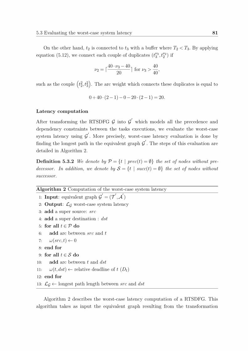
5.3 Evaluating the worst-case system latency 81
On the other hand, t2 is connected to t3 with a buffer where T2 < T3. By applyingequation (5.12), we connect each couple of duplicates (tν3
3 , tν22 ) if
ν2 = ⌈40 ·ν3−4020 ⌉ for ν3 >
4040 ,
such as the couple(t22, t2
3). The arc weight which connects these duplicates is equal to
0+40 · (2−1)−0−20 · (2−1) = 20.
Latency computation
After transforming the RTSDFG G into G ′ which models all the precedence anddependency constraints between the tasks executions, we evaluate the worst-casesystem latency using G ′
. More precisely, worst-case latency evaluation is done byfinding the longest path in the equivalent graph G ′
. The steps of this evaluation aredetailed in Algorithm 2.
Definition 5.3.2 We denote by P = t | prec(t) = ∅ the set of nodes without pre-decessor. In addition, we denote by S = t | succ(t) = ∅ the set of nodes withoutsuccessor.
Algorithm 2 Computation of the worst-case system latency1: Input: equivalent graph G ′ = (T ′
,A′)2: Output: LG worst-case system latency3: add a super source: src
4: add a super destination : dst
5: for all t ∈ P do6: add arc between src and t
7: ω(src, t)← 08: end for9: for all t ∈ S do
10: add arc between t and dst
11: ω(t,dst)← relative deadline of t (Dt)12: end for13: LG ← longest path length between src and dst
Algorithm 2 describes the worst-case latency computation of a RTSDFG. Thisalgorithm takes as input the equivalent graph resulting from the transformation

82 Real Time Synchronous Data Flow Graph (RTSDFG)
presented in Algorithm 1 and returns as output the value of the worst-case systemlatency. First, we add to G ′ two virtual nodes: a super source and a super destination(lines 3 and 4). Then, we connect src to each node t ∈ P with an arc whose weight isnull (from line 5 to 8). We connect each node t ∈ S to dst with an arc whose weight isequal to the relative deadline of t (from line 9 to 12). Adding these virtual nodes doesnot influence the time behavior of the system. Finally, we find the worst-case latencyvalue for the entire system by computing the length of the longest path between thevirtual nodes src and dst (line 13).
30
20
30
202020
20
20 20 20
00 0 0
4040
10
10
10
Fig. 5.13 Computation of the Worst-case latency of the RTSDFG depicted in Figure5.11.
In order to evaluate the worst-case latency of the RTSDG in Figure 5.11, weuse Algorithm 2 which takes as input the equivalent graph G ′ depicted in Figure5.12. We add two virtual nodes (src/dst) to the equivalent graph. Then, we connectsrc to each duplicate without predecessor P = t1
1, t21, t3
1, t11 with arcs whose weights
are null. On the other hand, we add arcs between each duplicate without successorS = t1
2, t32, t5
2, t13, t2
3, t33 and dst. Their weights are equal to the tasks relative deadline
(D2 = 10 and D3 = 20). Figure 5.13 depicts the resulting graph. Finally, in order to
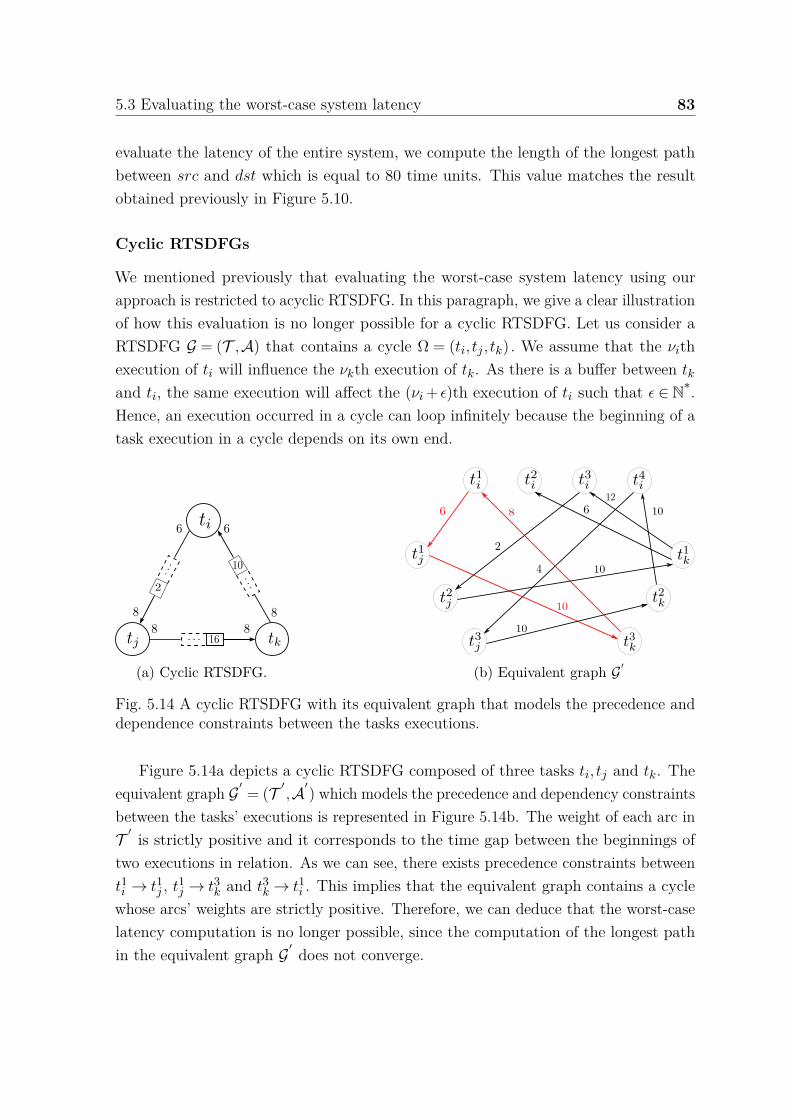
5.3 Evaluating the worst-case system latency 83
evaluate the latency of the entire system, we compute the length of the longest pathbetween src and dst which is equal to 80 time units. This value matches the resultobtained previously in Figure 5.10.
Cyclic RTSDFGs
We mentioned previously that evaluating the worst-case system latency using ourapproach is restricted to acyclic RTSDFG. In this paragraph, we give a clear illustrationof how this evaluation is no longer possible for a cyclic RTSDFG. Let us consider aRTSDFG G = (T ,A) that contains a cycle Ω = (ti, tj , tk) . We assume that the νithexecution of ti will influence the νkth execution of tk. As there is a buffer between tk
and ti, the same execution will affect the (νi + ϵ)th execution of ti such that ϵ ∈ N*.
Hence, an execution occurred in a cycle can loop infinitely because the beginning of atask execution in a cycle depends on its own end.
(a) Cyclic RTSDFG. (b) Equivalent graph G′
Fig. 5.14 A cyclic RTSDFG with its equivalent graph that models the precedence anddependence constraints between the tasks executions.
Figure 5.14a depicts a cyclic RTSDFG composed of three tasks ti, tj and tk. Theequivalent graph G ′ = (T ′
,A′) which models the precedence and dependency constraintsbetween the tasks’ executions is represented in Figure 5.14b. The weight of each arc inT ′ is strictly positive and it corresponds to the time gap between the beginnings oftwo executions in relation. As we can see, there exists precedence constraints betweent1i → t1
j , t1j → t3
k and t3k→ t1
i . This implies that the equivalent graph contains a cyclewhose arcs’ weights are strictly positive. Therefore, we can deduce that the worst-caselatency computation is no longer possible, since the computation of the longest pathin the equivalent graph G ′ does not converge.

84 Real Time Synchronous Data Flow Graph (RTSDFG)
Computation of the longest path
The NP-hardness of the longest path problem for arbitrary graphs can be shown usingthe reduction from Hamiltonian path problem. However, computing the longest pathin directed acyclic graphs (DAG in short) has a linear solution using a topologicalsorting. It can be computed by applying a linear time algorithm for shortest paths ina DAG [21] in which every weight is replaced by its negation. The complexity of thisalgorithm is O(n + m) where n is the number of nodes and m is the number of arcs ofthe graph. However, the complexity of transforming the RTSDFG into an equivalentgraph is not polynomial. The computation of this complexity is detailed in Section 7.2of Chapter 7.
In the next part of this chapter, we present two algorithms that compute respec-tively the upper and lower bounds of the system latency. The computation of thesebounds does not require the use of the equivalent graph which explicitly represents theprecedence and the dependency constraints between the tasks executions.
5.3.3 Upper bound
In order to evaluate the upper and lower bounds of the system latency, our approachconsists on transforming the RTSDFG into a weighted graph. The size of this latteris equal to the size of the original graph. In addition, the weight of each arc in theweighted graph corresponds to the time required to transfer the data between two taskin the worst (or best) case scenario.
Let us consider the RTSDFG buffer a = (ti, tj) with zi = Ti, zj = Tj and M0(a) itsinitial marking. We assume that a models all the communication constraints betweenthe two periodic communicating tasks ti = (ri,Ci,Di,Ti) and tj = (rj ,Cj ,Dj ,Tj). Ac-cording to our communication model presented in section 5.1.2, data are only availableat the deadline of the emitting task ti. Moreover, these data can only be consumedat the release date of the receiving task tj . On the other hand, the latency betweentwo communicating tasks is equal to the time gap between the deadline of ti and therelease date of tj . According to Theorem 5.2.1, the maximum latency between theexecutions of ti and tj can be written in the following format:
Lmax(ti, tj) = rj− ri +λ+Ti−max0,Ti−Tj−gcda−Di,
where λ =⌈
ri−rj+Di
gcda
⌉·gcda.

5.3 Evaluating the worst-case system latency 85
In order to compute the time required to transfer the data between ti and tj in theworst case scenario, two cases should be studied:
1. If Ti ≤ Tj ,
Lmax(ti, tj) = rj− ri +λ+Ti−gcda−Di.
After an execution of ti, tj can be executed at most one time. Hence, thetime required to ensure the data transfer between these tasks, in the worst casescenario, is equal to
Di +Lmax (ti, tj) = Di + rj− ri +λ+Ti−gcda−Di
= rj− ri +λ+Ti−gcda.
In our example in Figure 5.10 on page 75, t2 = (0,5,10,20) communicates witht3 = (0,10,20,40) where T2 < T3 and gcda = gcd(20,40) = 20. Hence, the timeneeded for the data transfer from t2 to t3, in the worst case scenario, is equal to
D2 +Lmax (t2, t3) = r3− r2 +λ+T2−gcda
= 0+ ⌈0+1020 ⌉ ·20+20−20
= 20 time units.
2. If Ti > Tj ,Lmax(ti, tj) = rj− ri +λ+Tj−gcda−Di.
After an execution of ti, tj can be executed at most ⌈ TiTj⌉ times. This means that at
most ⌈ TiTj⌉ executions of tj are totally depend on the execution of ti. Accordingly,
the time separating the beginnings of the first and the last executions of tj thatdepend on ti is equal to (⌈ Ti
Tj⌉−1) ·Tj time units. Hence, in order to ensure the
data transfer from ti to tj , the time required in the worst case scenario is equalto
Di +Lmax(ti, tj)+(⌈Ti
Tj⌉−1) ·Tj = rj− ri +λ−gcda + ⌈Ti
Tj⌉ ·Tj .
In the same example on page 75, t1 = (0,10,20,30) and t2 = (0,5,10,20) arecommunicating with T1 > T2 and gcda = gcd(30,20) = 10. Therefore, an execution

86 Real Time Synchronous Data Flow Graph (RTSDFG)
of t1 will affect at most ⌈T1T2⌉= ⌈30
20⌉= 2 executions of t2. Accordingly, the timeseparating the beginnings of the first and the last executions of t2 that totallydepend on the execution of t1 is equal to (2−1) ·20 time units. In the worst case,the time needed to transfer the data between these tasks is equal to
Di +Lmax(ti, tj)+(⌈Ti
Tj⌉−1) ·Tj = rj− ri +λ−gcda + ⌈Ti
Tj⌉ ·Tj
= 0+ ⌈0+2010 ⌉ ·10−10+2 ·20
= 50 time units.
In the next paragraph, we propose an algorithm covering the two cases below.
Latency upper bound computation
Algorithm 3 From RTSDFG to weighted graph Gmax
1: Input: RTSDFG G = (T ,A)2: Output: Weighted graph Gmax
3: arc weight: ω(e)4: substitute each task ti ∈ T by a node ti
5: substitute each buffer a = (ti, tj) ∈ A by an arc e = (ti, tj)6: for all a = (ti, tj) ∈ A do7: if Ti ≤ Tj then8: ω(e)← rj− ri +λ+Ti−gcda
9: else10: ω(e)← rj− ri +λ+ ⌈ Ti
Tj⌉ ·Tj−gcda
11: end if12: end for
Algorithm 3 converts a RTSDFG G = (T ,A) into a weighted graph Gmax havingthe same size. Each task ti ∈ T is represented by a node (line 4) and each buffera = (ti, tj) is represented by an arc e = (ti, tj) (line 5). The arc weight ω(e) correspondsto the time required for data transfer from ti to tj in the worst case scenario. Thisweight is computed in two different cases according to the values of the buffer produc-tion and consumption rates. The two cases are respectively represented in line 8 and 10.
In order to evaluate the upper bound of the system latency, we add to the resultinggraph Gmax two virtual nodes src and dst. Then, we connect src to each node without

5.3 Evaluating the worst-case system latency 87
predecessor with an arc whose weight is null. We also connect each node withoutsuccessor to dst with an arc whose weight is equal to the relative deadline of the sourcetask. We evaluate the latency upper bound by computing the longest path betweenthe virtual nodes (src and dst).
(a) Acyclic RTSDFG.
0
(b) Weighted graph Gmax
Fig. 5.15 Example of latency upper bound computation using the weighted graph Gmax
Consider the RTSFG in Figure 5.15a that models the communication constraintsbetween the executions of t1 = (0,10,20,30), t2 = (0,10,20,40) and t3 = (0,5,10,20).Figure 5.15b presents the weighted graph Gmax. In this graph, the weight of each arcconnecting two nodes corresponds to the time required to transfer the data betweenthese nodes in the worst case scenario. For example, the time required to ensure thecommunication between (t1, t3) ,(t1, t2) and (t3, t2) is respectively equal to 50,50 and20 time units.
Let P = t1 be the set of nodes that do not have any predecessor. In addition, letS = t2 be the set of nodes that do not have any successor. Two super nodes (src /dst) are added to Gmax. We connect src to t1 with an arc whose weight is null, and t2
to dst with an arc whose weight is equal to D2 = 20 time units. In order to evaluatethe latency upper bound, we compute the length of the longest path between src anddst which is equal to 90 time units.
5.3.4 Lower bound
Let ti = (ri,Ci,Di,Ti) and tj = (rj ,Cj ,Dj ,Tj) be two periodic communicating tasks.Let a = (ti, tj) be RTSDFG buffer that models all the communication constraintsbetween the tasks executions. According to Theorem 5.2.2, the minimum latencybetween the tasks executions is computed as follows:
Lmin(ti, tj) = rj− ri +λ−Di.
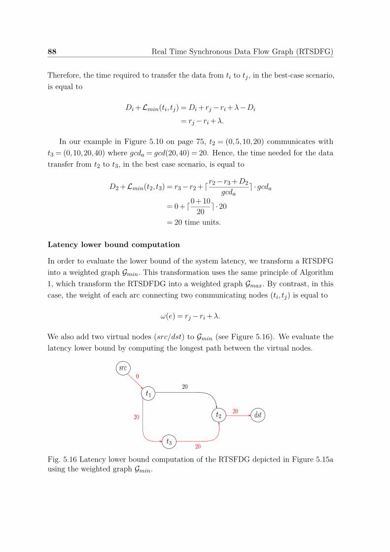
88 Real Time Synchronous Data Flow Graph (RTSDFG)
Therefore, the time required to transfer the data from ti to tj , in the best-case scenario,is equal to
Di +Lmin(ti, tj) = Di + rj− ri +λ−Di
= rj− ri +λ.
In our example in Figure 5.10 on page 75, t2 = (0,5,10,20) communicates witht3 = (0,10,20,40) where gcda = gcd(20,40) = 20. Hence, the time needed for the datatransfer from t2 to t3, in the best case scenario, is equal to
D2 +Lmin(t2, t3) = r3− r2 + ⌈r2− r3 +D2gcda
⌉ ·gcda
= 0+ ⌈0+1020 ⌉ ·20
= 20 time units.
Latency lower bound computation
In order to evaluate the lower bound of the system latency, we transform a RTSDFGinto a weighted graph Gmin. This transformation uses the same principle of Algorithm1, which transform the RTSDFDG into a weighted graph Gmax. By contrast, in thiscase, the weight of each arc connecting two communicating nodes (ti, tj) is equal to
ω(e) = rj− ri +λ.
We also add two virtual nodes (src/dst) to Gmin (see Figure 5.16). We evaluate thelatency lower bound by computing the longest path between the virtual nodes.
0
Fig. 5.16 Latency lower bound computation of the RTSFDG depicted in Figure 5.15ausing the weighted graph Gmin.
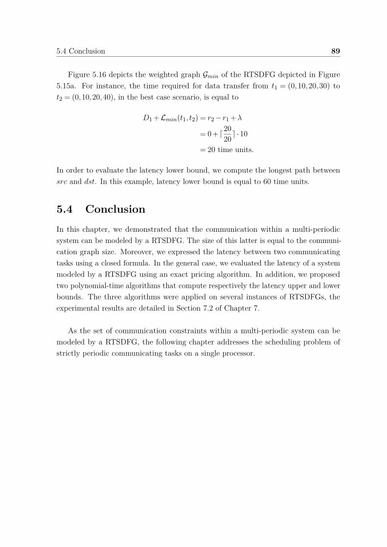
5.4 Conclusion 89
Figure 5.16 depicts the weighted graph Gmin of the RTSDFG depicted in Figure5.15a. For instance, the time required for data transfer from t1 = (0,10,20,30) tot2 = (0,10,20,40), in the best case scenario, is equal to
D1 +Lmin(t1, t2) = r2− r1 +λ
= 0+ ⌈2020⌉ ·10
= 20 time units.
In order to evaluate the latency lower bound, we compute the longest path betweensrc and dst. In this example, latency lower bound is equal to 60 time units.
5.4 ConclusionIn this chapter, we demonstrated that the communication within a multi-periodicsystem can be modeled by a RTSDFG. The size of this latter is equal to the communi-cation graph size. Moreover, we expressed the latency between two communicatingtasks using a closed formula. In the general case, we evaluated the latency of a systemmodeled by a RTSDFG using an exact pricing algorithm. In addition, we proposedtwo polynomial-time algorithms that compute respectively the latency upper and lowerbounds. The three algorithms were applied on several instances of RTSDFGs, theexperimental results are detailed in Section 7.2 of Chapter 7.
As the set of communication constraints within a multi-periodic system can bemodeled by a RTSDFG, the following chapter addresses the scheduling problem ofstrictly periodic communicating tasks on a single processor.


Chapter 6
Scheduling strictly periodic systemswith communication constraints
Preemptive real-time systems have received considerable research efforts in the real-time community, compared to non-preemptive systems. However, these latter areusually adopted in practical hard-real real time systems where missing deadlines maylead to catastrophic situations. Moreover, many industrial applications (e.g. avionicapplications) require strictly periodic tasks. This means that the tasks successiveexecutions admit periodic starting dates separated by the task period. This strictperiodicity is usually required at the system inputs and outputs, such as the sensorsand the actuators of a control/command applications.
In many hard real-time systems, communication is becoming increasingly indispens-able. Due to the tasks strict deadlines that must be met, communications between thetasks executions are implemented in a completely deterministic manner. Our approachmodels the communication requirements as precedence constraints between tasks. Moreprecisely, this approach consists of modeling the communications within multi-periodicsystems using RTSDFG formalisms.
In this chapter, we consider the mono-processor scheduling problem for non-preemptive strictly periodic systems subject to communication constraints. Section6.1 presents the non-preemptive strictly periodic model and its characteristics. Inaddition, it recalls the schedulability condition of two independent tasks on the sameprocessor. Section 6.2 defines the SDFG schedules, especially the periodic ones thatcombine an explicit description of starting dates and an easy implementation. Section6.3 introduces the schedulability condition of two non-preemptive strictly periodictasks with communication constraints. In order to solve the scheduling problem, an
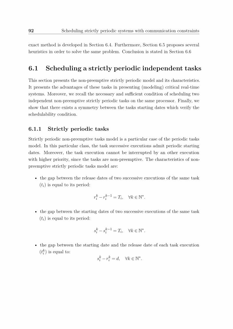
92 Scheduling strictly periodic systems with communication constraints
exact method is developed in Section 6.4. Furthermore, Section 6.5 proposes severalheuristics in order to solve the same problem. Conclusion is stated in Section 6.6
6.1 Scheduling a strictly periodic independent tasksThis section presents the non-preemptive strictly periodic model and its characteristics.It presents the advantages of these tasks in presenting (modeling) critical real-timesystems. Moreover, we recall the necessary and sufficient condition of scheduling twoindependent non-preemptive strictly periodic tasks on the same processor. Finally, weshow that there exists a symmetry between the tasks starting dates which verify theschedulability condition.
6.1.1 Strictly periodic tasks
Strictly periodic non-preemptive tasks model is a particular case of the periodic tasksmodel. In this particular class, the task successive executions admit periodic startingdates. Moreover, the task execution cannot be interrupted by an other executionwith higher priority, since the tasks are non-preemptive. The characteristics of non-preemptive strictly periodic tasks model are:
• the gap between the release dates of two successive executions of the same task(ti) is equal to its period:
rki − rk−1
i = Ti, ∀k ∈ N∗.
• the gap between the starting dates of two successive executions of the same task(ti) is equal to its period:
ski − sk−1
i = Ti, ∀k ∈ N∗.
• the gap between the starting date and the release date of each task execution(tk
i ) is equal to:sk
i − rki = d, ∀k ∈ N∗.
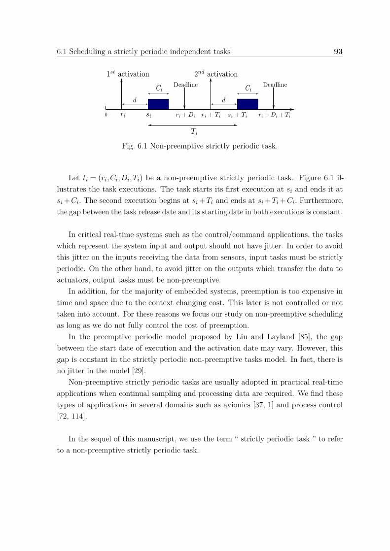
6.1 Scheduling a strictly periodic independent tasks 93
Fig. 6.1 Non-preemptive strictly periodic task.
Let ti = (ri,Ci,Di,Ti) be a non-preemptive strictly periodic task. Figure 6.1 il-lustrates the task executions. The task starts its first execution at si and ends it atsi +Ci. The second execution begins at si +Ti and ends at si +Ti +Ci. Furthermore,the gap between the task release date and its starting date in both executions is constant.
In critical real-time systems such as the control/command applications, the taskswhich represent the system input and output should not have jitter. In order to avoidthis jitter on the inputs receiving the data from sensors, input tasks must be strictlyperiodic. On the other hand, to avoid jitter on the outputs which transfer the data toactuators, output tasks must be non-preemptive.
In addition, for the majority of embedded systems, preemption is too expensive intime and space due to the context changing cost. This later is not controlled or nottaken into account. For these reasons we focus our study on non-preemptive schedulingas long as we do not fully control the cost of preemption.
In the preemptive periodic model proposed by Liu and Layland [85], the gapbetween the start date of execution and the activation date may vary. However, thisgap is constant in the strictly periodic non-preemptive tasks model. In fact, there isno jitter in the model [29].
Non-preemptive strictly periodic tasks are usually adopted in practical real-timeapplications when continual sampling and processing data are required. We find thesetypes of applications in several domains such as avionics [37, 1] and process control[72, 114].
In the sequel of this manuscript, we use the term “ strictly periodic task ” to referto a non-preemptive strictly periodic task.

94 Scheduling strictly periodic systems with communication constraints
6.1.2 Schedulabilty analysis of strictly periodic independenttasks
Considering a set of strictly periodic independent tasks T = t1, . . . , tn. Each taskti ∈ T is characterized by an activation period Ti, an execution time Ci and a startingdate (of the first execution) si. Since there is no precedence constraints between thetasks executions, we assume without loss of generality that si ∈ [0,Ti). We use theinterval Eνi
i (si) to characterize the execution time units occupied by the νith executionof ti having a starting date equals to si. The first execution interval of ti begins at si andends before si +Ci, hence E1
i (si) = [si, si +Ci). According to the task strict periodicity,the νith execution of ti begins at si + (νi−1) ·Ti and ends before si + (νi−1) ·Ti + Ci.
More formally, the execution time units for each task can be written as follows:
∀ti ∈ T ,∀νi ≥ 1, Eνii (si) = [si +(νi−1) ·Ti, si +(νi−1) ·Ti +Ci)
Let ti = (si,Ci,Ti) and tj = (sj ,Cj ,Tj) be two strictly periodic independent tasks.These tasks are schedulable on the same processor if and only if there is no overlappingbetween their executions. This means ∀(νi,νj) ∈ N∗2
,Eνii (si)∩E
νj
j (sj) = ∅. Therefore,a set of strictly periodic independent tasks T = t1, . . . , tn can be scheduled on thesame processor if and only if each tasks couple (ti, tj) can be scheduled on the sameprocessor. This condition can be written as follows:
∀(ti, tj)i =j
∀(νi,νj) ∈ N∗2,Eνi
i (si)∩Eνj
j (sj) = ∅. (6.1)
Although the previous equation (6.1) is a necessary and sufficient condition, itcannot be directly used to solve the scheduling problem of two tasks. Indeed, equation(6.1) requires the computation of the time units intervals occupied by all the tasksexecutions. However, the number of the tasks execution can increase exponentiallyand this is unacceptable in practice. Theorem 6.1.1 provides a schedulability conditionwithout computing the interval execution time units occupied by all the tasks executions.This theorem was first proposed by Korst et al. [80]. More recently, Al Sheikh at al.[1] and Chen et al. [26] proved that this theorem does not require that the start dateof the first task has to be smaller than the start date of the second one. This is donefollowing the fact that (−a) mod (b) = b− (a) mod b.
Theorem 6.1.1 Two strictly periodic independent tasks ti = (si,Ci,Ti) and tj =(sj ,Cj ,Tj) are schedulable on the same processor if and only if

6.1 Scheduling a strictly periodic independent tasks 95
Ci ≤ (sj− si) mod (gij)≤ gij−Cj , (6.2)
where gij = gcd(Ti,Tj).
Corollary 6.1.1 results from theorem 6.1.1. It gives a necessary and sufficientcondition for scheduling the tasks on the same processor when their starting dates canbe freely assigned by the designer.
Corollary 6.1.1 [80] The executions of two periodic independent tasks ti = (Ci,Ti)and tj = (Cj ,Tj) can be scheduled on the same processor if and only if
Ci +Cj ≤ gij , (6.3)
where gij = gcd(Ti,Tj).
Example 6.1.1 Let ti = (si,Ci,Ti) and tj = (sj ,Cj ,Tj) be two independent strictlyperiodic tasks. We suppose that Ti = 30, Tj = 40 time units, Ci = Cj = 5 time units,and their starting dates are respectively equal to si = 0 and sj = 5 time units. Figure6.2a represents the tasks executions during their hyper period. We notice that there isno overlapping between the tasks executions (see Figure 6.2b). Therefore, ti and tj
can be scheduled on the same processor. We can verify this result (without computingthe tasks executions), by applying equation (6.2) as follows:
Ci ≤5≤
(sj− si) mod (gij)(5−0) mod (10)
≤ gij−Cj
≤ 10−5,
where gij = gcd(30,40) = 10 time units.
(a) Tasks executions. (b) Non overlapping between executions.
Fig. 6.2 Scheduling two strictly periodic tasks ti = (0,5,30) and tj = (5,5,40) on thesame processor.

96 Scheduling strictly periodic systems with communication constraints
Symmetry
Let ti = (si,Ci,Ti) and tj = (sj ,Cj ,Tj) be two strictly periodic independent tasks. Thedifference between the tasks starting dates (sj− si) can be written as follows:
sj− si = δij +kij ·gij , (6.4)
where δij = (sj− si) mod gij and kij = ⌊sj−si
gij⌋, with kij ∈ Z.
On the other hand, the difference between the tasks starting dates (si− sj) can bewritten as follows:
si− sj = δji +kji ·gij , (6.5)
where δji = (si− sj) mod gij and kji = ⌊si−sj
gij⌋, with kji ∈ Z. According to the fact
that (−a) mod (b) = b− (a) mod (b) with a,b > 0, we can deduce that
δji = gij− δij .
Therefore, the equation (6.4) and (6.5) can also be written as follows:
sj− si = δij +kij ·gij
si− sj = gij− δij +kji ·gij .
By summing these equalities, we obtain
kij ·gij +(kji +1) ·gij = 0
Hence, we can deduce thatkij +kji =−1.
Finally, we can deduce a symmetry between δij and δji on one hand, and betweenkij and kji on the other hand. This implies that if there exists si and sj which verifythe equality (6.4) then these dates will also verify equality (6.5).
Let us consider the strictly periodic tasks ti = (0,5,30) and tj = (5,5,40) of ourprevious example. We notice that si and sj verify equation (6.4) with δij = 5 andkij = 0. In addition, these dates verify equation (6.5) with δji = gij− δij = 10−5 = 5and kji =−1−kij =−1.
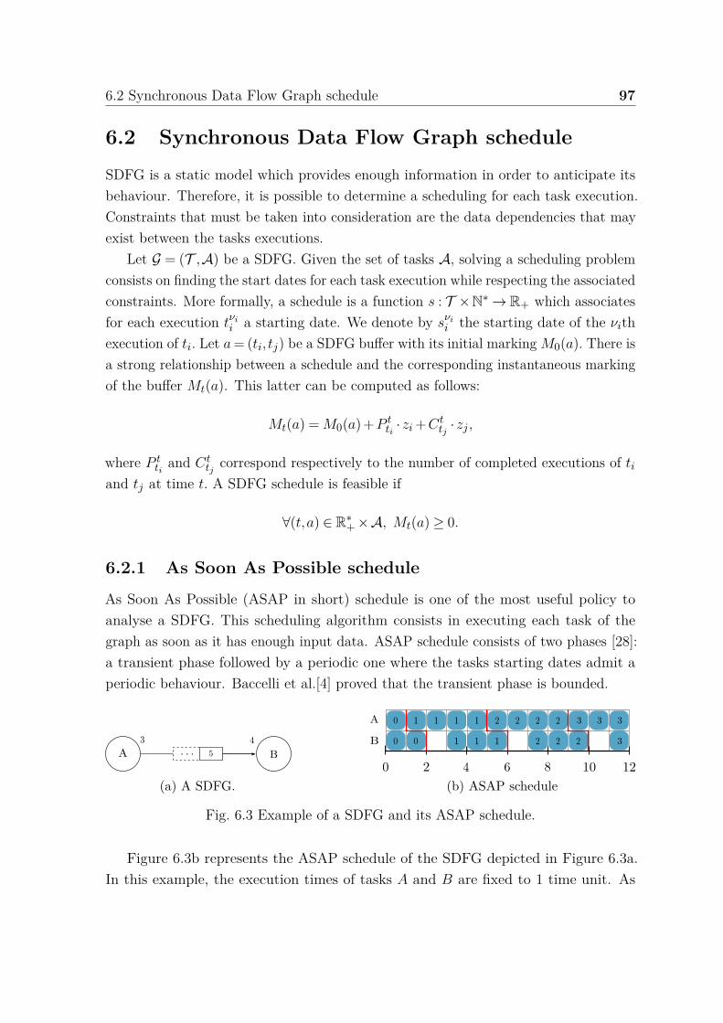
6.2 Synchronous Data Flow Graph schedule 97
6.2 Synchronous Data Flow Graph scheduleSDFG is a static model which provides enough information in order to anticipate itsbehaviour. Therefore, it is possible to determine a scheduling for each task execution.Constraints that must be taken into consideration are the data dependencies that mayexist between the tasks executions.
Let G = (T ,A) be a SDFG. Given the set of tasks A, solving a scheduling problemconsists on finding the start dates for each task execution while respecting the associatedconstraints. More formally, a schedule is a function s : T ×N∗→ R+ which associatesfor each execution tνi
i a starting date. We denote by sνii the starting date of the νith
execution of ti. Let a = (ti, tj) be a SDFG buffer with its initial marking M0(a). There isa strong relationship between a schedule and the corresponding instantaneous markingof the buffer Mt(a). This latter can be computed as follows:
Mt(a) = M0(a)+P tti· zi +Ct
tj· zj ,
where P tti
and Cttj
correspond respectively to the number of completed executions of ti
and tj at time t. A SDFG schedule is feasible if
∀(t,a) ∈ R∗+×A, Mt(a)≥ 0.
6.2.1 As Soon As Possible schedule
As Soon As Possible (ASAP in short) schedule is one of the most useful policy toanalyse a SDFG. This scheduling algorithm consists in executing each task of thegraph as soon as it has enough input data. ASAP schedule consists of two phases [28]:a transient phase followed by a periodic one where the tasks starting dates admit aperiodic behaviour. Baccelli et al.[4] proved that the transient phase is bounded.
(a) A SDFG. (b) ASAP schedule
Fig. 6.3 Example of a SDFG and its ASAP schedule.
Figure 6.3b represents the ASAP schedule of the SDFG depicted in Figure 6.3a.In this example, the execution times of tasks A and B are fixed to 1 time unit. As
98 Scheduling strictly periodic systems with communication constraints
we can see in Figure 6.3b, the transition phase is limited to one execution of A andtwo executions of B (executions are marked by zeros). This phase is followed by aperiodic phase where an execution pattern is repeated for each period (delimited byred lines). This pattern consists on executing task A four times and task B three times.The tasks’ executions are marked according to the period number. For example, theexecutions marked by 1 correspond to the tasks’ executions of the first period.
In general, the ASAP strategy does not guarantee a bounded marking. In fact,ensuring a bounded marking using ASAP strategy is restricted to some classes ofstrongly connected graphs. In addition, the drawback of the ASAP strategy forscheduling a SDFG, is the dependency from the SDFG repetition vector rather thanits size (|T |).
6.2.2 Periodic schedule
SDFGs are usually used to model applications that can be executed infinitely. Hence,the SDFG schedule must fix an infinite number of execution starting dates. In orderto avoid this kind of issues, authors in [90, 12] were interested in the SDFG periodicschedules. They characterize each SDFG task ti by an activation period (ωi ∈R∗
+) anda starting date of the first execution (si).
Definition 6.2.1 Let G = (T ,A) be a SDFG. A SDFG schedule is periodic if eachtask ti ∈ T has a period ωi such that
∀νi ≥ 1, sνii = si +(νi−1) ·ωi.
si is the starting date of the first execution of ti. The successive executions of ti arethen repeated every ωi time units.
Let G = (T ,A) be a normalized SDFG. Considering a task ti ∈A, let a be an outputbuffer of ti. Every ωi time units, zi tokens are produced in the buffer a. Hence, onaverage, a token is produced every ωi
zitime units. This ratio is called average token flow
time. Considering that all the tasks have the same average token flow time, Marchettiand Munier [90] prove that feasible periodic schedules satisfy linear inequalities. Theydefined a condition on the starting dates of the tasks first executions in order to fulfilthe precedence constraints induced by the buffers.
Theorem 6.2.1 [90] Let G = (T ,A) be a normalized SDFG. For any periodic schedule,there exists a strictly positive rational K ∈Q∗
+ such that, for each task ti ∈ T , ωizi
= K.
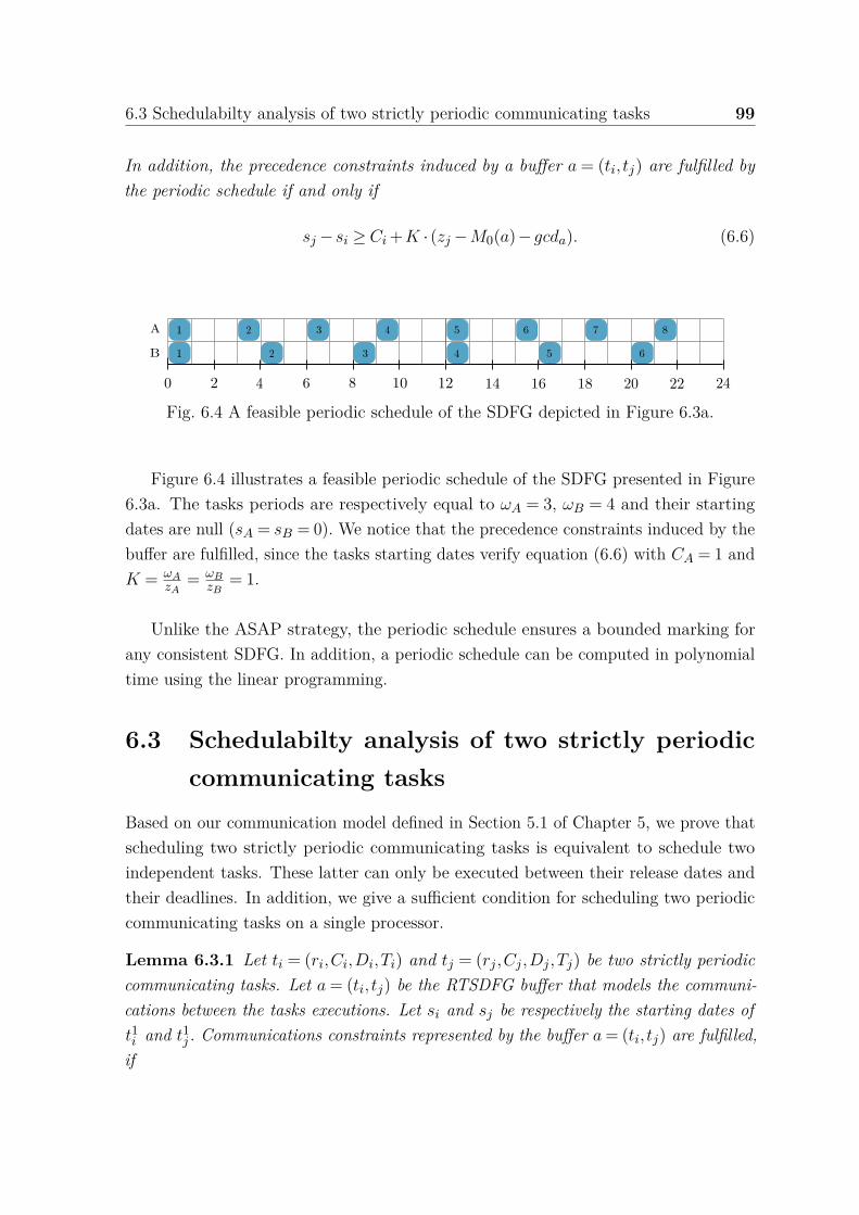
6.3 Schedulabilty analysis of two strictly periodic communicating tasks 99
In addition, the precedence constraints induced by a buffer a = (ti, tj) are fulfilled bythe periodic schedule if and only if
sj− si ≥ Ci +K · (zj−M0(a)−gcda). (6.6)
Fig. 6.4 A feasible periodic schedule of the SDFG depicted in Figure 6.3a.
Figure 6.4 illustrates a feasible periodic schedule of the SDFG presented in Figure6.3a. The tasks periods are respectively equal to ωA = 3, ωB = 4 and their startingdates are null (sA = sB = 0). We notice that the precedence constraints induced by thebuffer are fulfilled, since the tasks starting dates verify equation (6.6) with CA = 1 andK = ωA
zA= ωB
zB= 1.
Unlike the ASAP strategy, the periodic schedule ensures a bounded marking forany consistent SDFG. In addition, a periodic schedule can be computed in polynomialtime using the linear programming.
6.3 Schedulabilty analysis of two strictly periodiccommunicating tasks
Based on our communication model defined in Section 5.1 of Chapter 5, we prove thatscheduling two strictly periodic communicating tasks is equivalent to schedule twoindependent tasks. These latter can only be executed between their release dates andtheir deadlines. In addition, we give a sufficient condition for scheduling two periodiccommunicating tasks on a single processor.
Lemma 6.3.1 Let ti = (ri,Ci,Di,Ti) and tj = (rj ,Cj ,Dj ,Tj) be two strictly periodiccommunicating tasks. Let a = (ti, tj) be the RTSDFG buffer that models the communi-cations between the tasks executions. Let si and sj be respectively the starting dates oft1i and t1
j . Communications constraints represented by the buffer a = (ti, tj) are fulfilled,if

100 Scheduling strictly periodic systems with communication constraints
si ∈ [ri, ri +Di−Ci] and sj ∈ [rj , rj +Dj−Cj ].
Proof: Let a = (ti, tj) be the RTSDFG buffer that models the set of communi-cation constraints between the strictly periodic tasks ti = (ri,Ci,Di,Ti) and tj =(rj ,Cj ,Dj ,Tj). Let sνi
i and sνj
j be respectively the starting dates of tνii and t
νj
j . Accord-ing to corollary 5.1.1, communication constraints induced by the buffer a are fulfilled,if
∀νi ≥ 1, sνii ∈ [ri +(νi−1) ·Ti, ri +Di−Ci +(νi−1) ·Ti] and,
∀νj ≥ 1, sνj
j ∈ [rj +(νj−1) ·Tj , rj +Dj−Cj +(νj−1) ·Tj ].
On the other hand, according to the task strict periodicity, the execution starting datessνi
i and sνj
j can be computed in function of the tasks first executions (si and sj) asfollowing:
sνii = si +(νi−1) ·Ti
sνj
i = sj +(νj−1) ·Tj .
Consequently, it is sufficient that si ∈ [ri, ri +Di−Ci] and sj ∈ [rj , rj +Dj−Cj ] (forνi = νj = 1) to ensure that all communications constraints induced by the buffer a aresatisfied.
Fig. 6.5 Communications constraints between the executions of two strictly periodictasks ti = (10,3,15,30) and tj = (0,4,15,40).
Example 6.3.1 Let ti = (10,3,15,30) and tj = (0,4,15,40) be two strictly periodiccommunicating tasks. Figure 6.5 represents the communications between the tasksexecutions. We suppose that the tasks start their executions respectively at si = 10

6.3 Schedulabilty analysis of two strictly periodic communicating tasks 101
and sj = 5 time units. Communication constraints are fulfilled, since the first executionof each task is accomplished between its release date and its deadline (si ∈ [10,22] andsj ∈ [0,11]).
Theorem 6.3.1 Let ti = (ri,Ci,Di,Ti) and tj = (rj ,Cj ,Dj ,Tj) be two strictly periodiccommunicating tasks. Let si and sj be respectively the starting dates of t1
i and t1j such
that si ∈ [ri, ri + Di−Ci] and sj ∈ [rj , rj + Dj−Cj ]. These tasks can be scheduled onthe same processor if and only if
Ci ≤ (sj− si) mod gij ≤ gij−Cj ,
where gij = gcd(Ti,Tj).
Proof: Considering ti = (ri,Ci,Di,Ti) and tj = (rj ,Cj ,Dj ,Tj) two strictly periodiccommunicating tasks. Let a = (ti, tj) be the RTSDFG buffer that models the commu-nication constraints between the tasks executions. Let si and sj be respectively thestarting dates of t1
i and t1j such that si ∈ [ri, ri + Di−Ci] and sj ∈ [rj , rj + Dj−Cj ].
Consequently, according to lemma 6.3.1, communications constraints induced by theRTSDFG buffer a = (ti, tj) are fulfilled. Hence, we can deduce that tasks ti = (si,Ci,Ti)and tj = (sj ,Cj ,Tj) can be considered as independent tasks, since the starting dates oftheir first executions si and sj satisfy the communications constraints.
On the other hand, two strictly periodic independent tasks are scheduled on thesame processor if and only if there is no overlapping between their executions. Accordingto theorem 6.1.1, these tasks can be executed on the same processor if and only if thestarting dates of their first executions satisfy the following equation:
Ci ≤ (sj− si) mod gij ≤ gij−Cj .
Let us consider the strictly periodic communicating tasks ti = (10,3,15,30) andtj = (0,4,15,40) of the example in Figure 6.5. Tasks are executed between theirrelease dates and their deadlines. Therefore, communication constraints between theirexecutions are fulfilled. Accordingly, these tasks can be considered as independentones. Moreover, we notice that the tasks starting dates si = 10 and sj = 5 verify thecondition of scheduling two independent tasks on the same processor (equation (6.2)):
Ci ≤3≤
(sj− si) mod gij
(5−10) mod 10≤ gij−Cj
≤ 10−4.
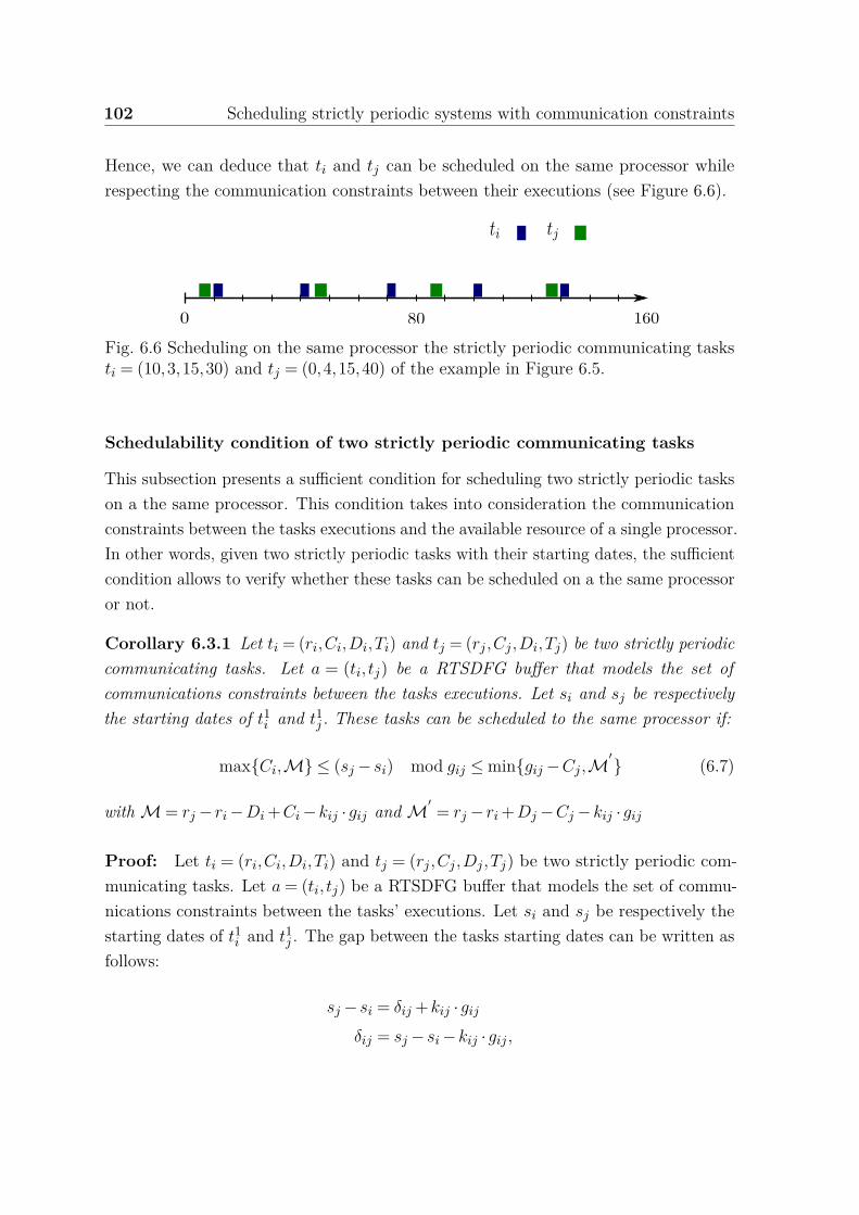
102 Scheduling strictly periodic systems with communication constraints
Hence, we can deduce that ti and tj can be scheduled on the same processor whilerespecting the communication constraints between their executions (see Figure 6.6).
Fig. 6.6 Scheduling on the same processor the strictly periodic communicating tasksti = (10,3,15,30) and tj = (0,4,15,40) of the example in Figure 6.5.
Schedulability condition of two strictly periodic communicating tasks
This subsection presents a sufficient condition for scheduling two strictly periodic taskson a the same processor. This condition takes into consideration the communicationconstraints between the tasks executions and the available resource of a single processor.In other words, given two strictly periodic tasks with their starting dates, the sufficientcondition allows to verify whether these tasks can be scheduled on a the same processoror not.
Corollary 6.3.1 Let ti = (ri,Ci,Di,Ti) and tj = (rj ,Cj ,Di,Tj) be two strictly periodiccommunicating tasks. Let a = (ti, tj) be a RTSDFG buffer that models the set ofcommunications constraints between the tasks executions. Let si and sj be respectivelythe starting dates of t1
i and t1j . These tasks can be scheduled to the same processor if:
maxCi,M≤ (sj− si) mod gij ≤mingij−Cj ,M′ (6.7)
with M= rj− ri−Di +Ci−kij ·gij and M′ = rj− ri +Dj−Cj−kij ·gij
Proof: Let ti = (ri,Ci,Di,Ti) and tj = (rj ,Cj ,Dj ,Tj) be two strictly periodic com-municating tasks. Let a = (ti, tj) be a RTSDFG buffer that models the set of commu-nications constraints between the tasks’ executions. Let si and sj be respectively thestarting dates of t1
i and t1j . The gap between the tasks starting dates can be written as
follows:
sj− si = δij +kij ·gij
δij = sj− si−kij ·gij ,
6.3 Schedulabilty analysis of two strictly periodic communicating tasks 103
where δij = (sj−si) mod gij and kij = ⌊sj−si
gij⌋. According to theorem 6.1.1, two strictly
periodic independent tasks can be scheduled on the same processor if
Ci ≤Ci ≤
δij
(sj− si)−kij ·gij
≤ gij−Cj
≤ gij−Cj .(6.8)
On the other hand, there exists a set of communication constraints between theexecutions of ti and those of tj . According to lemma 6.3.1, communication constraintsbetween the tasks’ executions are fulfilled if the starting dates of their first executionsbelong to the following intervals:
ri ≤ si ≤ ri +Di−Ci
rj ≤ sj ≤ rj +Dj−Cj .
Hence, the gap between si and sj can be written as follows:
rj− ri−Di +Ci ≤ sj− si ≤ rj− ri +Dj−Cj
Therefore, the communication constraints between the tasks’ executions are fulfilled ifδij = (sj− si)−kij ·gij satisfy the following inequality:
rj− ri−Di +Ci−kij ·gij ≤ (sj− si)−kij ·gij ≤ rj− ri +Dj−Cj−kij ·gij (6.9)
By combining equations (6.8) and (6.9), we can deduce that two strictly periodiccommunicating tasks can be scheduled on the same processor if
maxCi, rj− ri−Di +Ci−kij ·gij ≤ δij ≤mingij−Cj , rj− ri +Dj−Cj−kij ·gij
Considering the strictly periodic communicating tasks ti = (10,3,15,30) and tj =(0,4,15,40). We assume that the tasks starting dates are respectively equal to si = 10and sj = 5. Scheduling these tasks on the same processor can be verified by applyingequation (6.7) as follows:
maxCi,M≤max3,−12 ≤
(sj− si) mod gij
(5−10) mod 10≤mingij−Cj ,M
′
≤min10−4,11,
with M= 0−10−15+3− (−1) ·10 =−12 and M′ = 0−10+15−4− (−1) ·10 = 11.
104 Scheduling strictly periodic systems with communication constraints
6.4 Optimal algorithm: Integer linear programmingformulation
A linear programming (LP in short) problem consists on maximizing or minimizinga linear function, subject to a finite number of linear constraints. These latter maybe equalities or inequalities. The problem feasible region is a convex polytope whichis defined by linear inequalities. Its objective function is a real-valued affine functiondefined on this polytope. A linear programming algorithm consists on searchingthrough the polytope vertices in order to find a point (on this polytope) where theobjective function has the smallest or the largest value if such a point exists. The linearprogramming problem was first introduced by Kantorovich [68] who also proposed amethod for solving it. The well know Simplex method, which is an important resolutionmethod dedicated to solve linear programs, was introduced by Dantzig [31]. The LPproblem can be solved using the Simplex method if there are no restrictions on thevariables types.
An integer linear programming (ILP in short) is a linear program with additionalconstraint which requires that all the variables are restricted to integer values. Whenthe integer restriction is applied only to a subset of the variables, the problem is definedas Mixed Integer Linear Programming (MILP in short). Several exact algorithms arededicated to solve these problems such as branch-and-bound [82], branch-and-cut [63],branch-and-price [105] and cutting-plane [88]. Moreover, these linear programmingalgorithms are known to be exact.
In this thesis, we need to answer the following question:For a given set of strictly periodic tasks, these latter can be scheduled on the same
processor, assuming that the tasks communicate with each other and can not be pre-empted?
In this section, an exact algorithm is suggested for the mono-processor schedulingproblem. This latter consists of scheduling a set of strictly periodic communicatingtasks on a single processor. Our approach used the mixed integer linear programmingformulation in order to build an exact framework. Our MILP formulation seeks afeasible solution that satisfies the constraints induced by the communications andavailable resource of a single processor without having any objective function.
Consider N = t1, . . . , tn a set of strictly periodic communicating tasks. LetG = (T ,A) be the RTSDFG which models all the communications constraints between

6.4 Optimal algorithm: Integer linear programming formulation 105
the tasks executions. According to lemma 6.3.1, the set of communication constraintsis fulfilled if the starting date of the first execution (si) of each task belongs to thefollowing interval:
∀ti ∈ T , si ∈ [ri, ri +Di−Ci].
In our study, we distinguish two cases: fixed and flexible intervals.
6.4.1 Fixed intervals
In this subsection, we presents the MILP formulation of the fixed intervals case,where each task ti = (ri,Ci,Di,Ti) can only start its first execution during the interval[ri, ri +Di−Ci]. Solving the MILP seeks to find a feasible solution if such one exists.A feasible solution is composed of a set of starting dates which verify simultaneouslythe communication and the resource constraints. Prior to presentation of the generalmodel, we present a list of constants and variables used in the MILP formulation.
Constants
• ri : Release date of the task first execution (t1i ).
• Ci : Execution time of task ti.
• Di : Relative deadline of task ti.
Variables
• si : Starting date of the task’s first execution (t1i ).
• δi,j : For each pair of tasks (ti, tj), δij corresponds to the time interval which isallowed to occupy without interfering with each other.
• ki,j : For each pair of tasks (ti, tj), ki,j corresponds to the number of intervals oflength gij separating the starting dates of the tasks’ first executions
Constraints
• Communication constraints: According to lemma 6.3.1, communication con-straints between the tasks executions are fulfilled if the first starting date of eachtask execution belongs to the following interval
∀ti ∈ T , ri ≤ si ≤ ri +Di−Ci
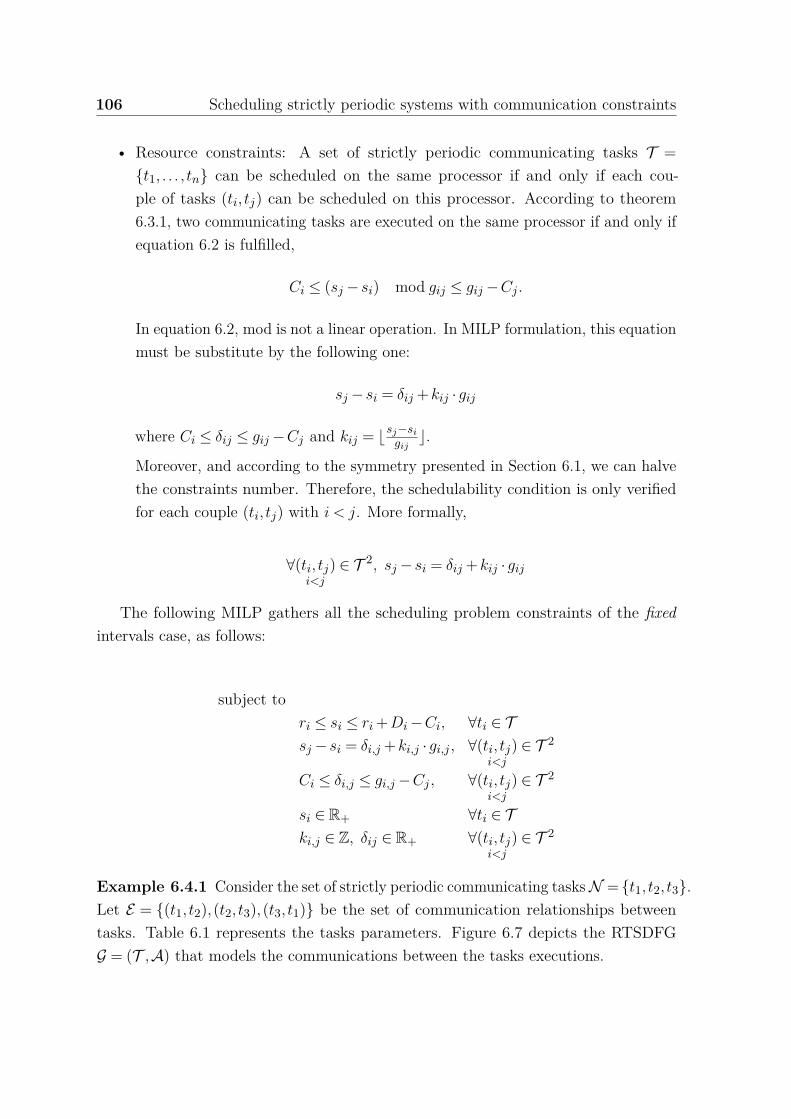
106 Scheduling strictly periodic systems with communication constraints
• Resource constraints: A set of strictly periodic communicating tasks T =t1, . . . , tn can be scheduled on the same processor if and only if each cou-ple of tasks (ti, tj) can be scheduled on this processor. According to theorem6.3.1, two communicating tasks are executed on the same processor if and only ifequation 6.2 is fulfilled,
Ci ≤ (sj− si) mod gij ≤ gij−Cj .
In equation 6.2, mod is not a linear operation. In MILP formulation, this equationmust be substitute by the following one:
sj− si = δij +kij ·gij
where Ci ≤ δij ≤ gij−Cj and kij = ⌊sj−si
gij⌋.
Moreover, and according to the symmetry presented in Section 6.1, we can halvethe constraints number. Therefore, the schedulability condition is only verifiedfor each couple (ti, tj) with i < j. More formally,
∀(ti, tj)i<j
∈ T 2, sj− si = δij +kij ·gij
The following MILP gathers all the scheduling problem constraints of the fixedintervals case, as follows:
subject tori ≤ si ≤ ri +Di−Ci, ∀ti ∈ Tsj− si = δi,j +ki,j ·gi,j , ∀(ti, tj)
i<j∈ T 2
Ci ≤ δi,j ≤ gi,j−Cj , ∀(ti, tj)i<j
∈ T 2
si ∈ R+ ∀ti ∈ Tki,j ∈ Z, δij ∈ R+ ∀(ti, tj)
i<j∈ T 2
Example 6.4.1 Consider the set of strictly periodic communicating tasksN = t1, t2, t3.Let E = (t1, t2),(t2, t3),(t3, t1) be the set of communication relationships betweentasks. Table 6.1 represents the tasks parameters. Figure 6.7 depicts the RTSDFGG = (T ,A) that models the communications between the tasks executions.
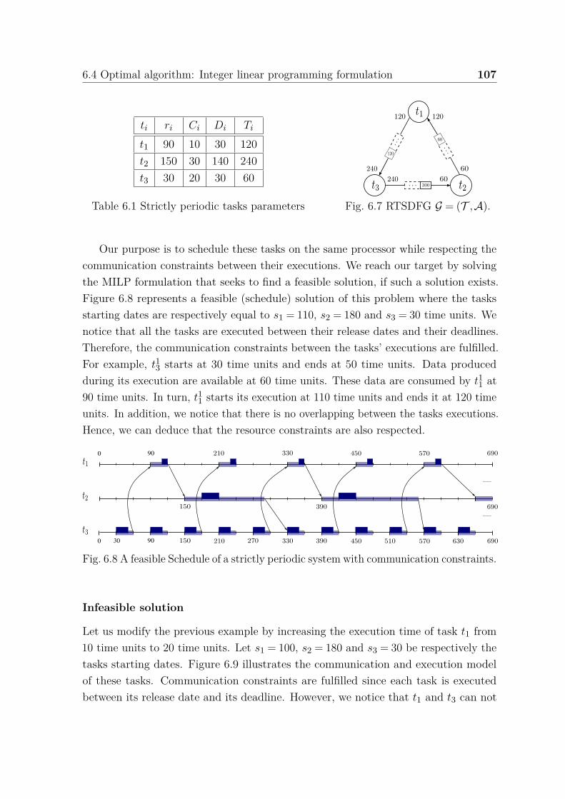
6.4 Optimal algorithm: Integer linear programming formulation 107
ti ri Ci Di Ti
t1 90 10 30 120t2 150 30 140 240t3 30 20 30 60
Table 6.1 Strictly periodic tasks parameters Fig. 6.7 RTSDFG G = (T ,A).
Our purpose is to schedule these tasks on the same processor while respecting thecommunication constraints between their executions. We reach our target by solvingthe MILP formulation that seeks to find a feasible solution, if such a solution exists.Figure 6.8 represents a feasible (schedule) solution of this problem where the tasksstarting dates are respectively equal to s1 = 110, s2 = 180 and s3 = 30 time units. Wenotice that all the tasks are executed between their release dates and their deadlines.Therefore, the communication constraints between the tasks’ executions are fulfilled.For example, t1
3 starts at 30 time units and ends at 50 time units. Data producedduring its execution are available at 60 time units. These data are consumed by t1
1 at90 time units. In turn, t1
1 starts its execution at 110 time units and ends it at 120 timeunits. In addition, we notice that there is no overlapping between the tasks executions.Hence, we can deduce that the resource constraints are also respected.
0 30 90
900
Fig. 6.8 A feasible Schedule of a strictly periodic system with communication constraints.
Infeasible solution
Let us modify the previous example by increasing the execution time of task t1 from10 time units to 20 time units. Let s1 = 100, s2 = 180 and s3 = 30 be respectively thetasks starting dates. Figure 6.9 illustrates the communication and execution modelof these tasks. Communication constraints are fulfilled since each task is executedbetween its release date and its deadline. However, we notice that t1 and t3 can not
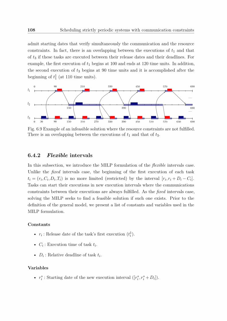
108 Scheduling strictly periodic systems with communication constraints
admit starting dates that verify simultaneously the communication and the resourceconstraints. In fact, there is an overlapping between the executions of t1 and thatof t3 if these tasks are executed between their release dates and their deadlines. Forexample, the first execution of t1 begins at 100 and ends at 120 time units. In addition,the second execution of t3 begins at 90 time units and it is accomplished after thebeginning of t1
1 (at 110 time units).
0 30 90
900
Fig. 6.9 Example of an infeasible solution where the resource constraints are not fulfilled.There is an overlapping between the executions of t1 and that of t3.
6.4.2 Flexible intervals
In this subsection, we introduce the MILP formulation of the flexible intervals case.Unlike the fixed intervals case, the beginning of the first execution of each taskti = (ri,Ci,Di,Ti) is no more limited (restricted) by the interval [ri, ri + Di−Ci].Tasks can start their executions in new execution intervals where the communicationsconstraints between their executions are always fulfilled. As the fixed intervals case,solving the MILP seeks to find a feasible solution if such one exists. Prior to thedefinition of the general model, we present a list of constants and variables used in theMILP formulation.
Constants
• ri : Release date of the task’s first execution (t1i ).
• Ci : Execution time of task ti.
• Di : Relative deadline of task ti.
Variables
• r∗i : Starting date of the new execution interval ([r∗
i , r∗i +Di]).
6.4 Optimal algorithm: Integer linear programming formulation 109
• si : Starting date of the task first execution (t1i ).
• δi,j : For each pair of tasks (ti, tj), δij corresponds to the time interval which isallowed to occupy without interfering with each other.
• ki,j : For each pair of tasks (ti, tj), ki,j corresponds to the number of intervals oflength gij separating the starting dates of the tasks’ first executions
Constraints
• Communication constraints: According to theorem 5.1.1 in section 5.1 of chapter 5,the set of communication constraints between two periodic tasks ti = (ri,Ci,Di,Ti)and tj = (rj ,Cj ,Dj ,Tj) is modeled by a RTSDFG buffer a = (ti, tj). Its productionand consumption rates are respectively equal to zi = Ti and zj = Tj and its initialmarking is equal to M0(a). Moreover, and according to theorem 6.2.1, theprecedence constraints induced by the buffer a = (ti, tj) are fulfilled by a periodicschedule if and only if
sj− si ≥ Ci +K · (zj−M0(a)−gcda),
where K = Tizi
= Tj
zj∈Q∗
+.
In our case, K is equal to Tizi
= Tj
zj= 1. The set of communications modeled by
the RTSDFG buffer is build according to the task’s release dates (ri) and theirrelative deadlines (Di). In fact, a RTSDFG’s task corresponds to the interval([ri, ri + Di]) during which the strictly periodic ti task is executed. Therefore,the starting date of the RTSDFG task can be considered as the starting date ofthe new execution interval (r∗
i ). Accordingly, precedence constraints between thenew execution intervals are fulfilled if and only if
∀a = (ti, tj) ∈ A, r∗j − r∗
i ≥Di +(Tj−M0(a)−gcda).
Then, the new execution interval must begin after the task release date,
∀ti ∈ T , r∗i ≥ ri.
Finally, and according to lemma 6.3.1, communications constraints between thetasks executions are fulfilled if the starting dates of their first execution belongs
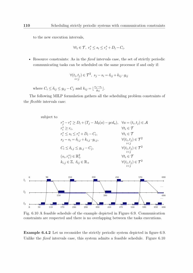
110 Scheduling strictly periodic systems with communication constraints
to the new execution intervals,
∀ti ∈ T , r∗i ≤ si ≤ r∗
i +Di−Ci.
• Resource constraints: As in the fixed intervals case, the set of strictly periodiccommunicating tasks can be scheduled on the same processor if and only if:
∀(ti, tj)i<j
∈ T 2, sj− si = δij +kij ·gij
where Ci ≤ δij ≤ gij−Cj and kij = ⌊sj−si
gij⌋.
The following MILP formulation gathers all the scheduling problem constraints ofthe flexible intervals case:
subject tor∗
j − r∗i ≥Di +(Tj−M0(a)−gcda), ∀a = (ti, tj) ∈ A
r∗i ≥ ri, ∀ti ∈ T
r∗i ≤ si ≤ r∗
i +Di−Ci, ∀ti ∈ Tsj− si = δi,j +ki,j ·gi,j , ∀(ti, tj)
i<j∈ T 2
Ci ≤ δi,j ≤ gi,j−Cj , ∀(ti, tj)i<j
∈ T 2
(si, r∗i ) ∈ R2
+ ∀ti ∈ Tki,j ∈ Z, δij ∈ R+ ∀(ti, tj)
i<j∈ T 2
0
900
Fig. 6.10 A feasible schedule of the example depicted in Figure 6.9. Communicationconstraints are respected and there is no overlapping between the tasks executions.
Example 6.4.2 Let us reconsider the strictly periodic system depicted in figure 6.9.Unlike the fixed intervals case, this system admits a feasible schedule. Figure 6.10
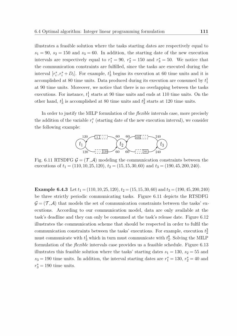
6.4 Optimal algorithm: Integer linear programming formulation 111
illustrates a feasible solution where the tasks starting dates are respectively equal tos1 = 90, s2 = 150 and s3 = 60. In addition, the starting date of the new executionintervals are respectively equal to r∗
1 = 90, r∗2 = 150 and r∗
3 = 50. We notice thatthe communication constraints are fulfilled, since the tasks are executed during theinterval [r∗
i , r∗i + Di]. For example, t1
3 begins its execution at 60 time units and it isaccomplished at 80 time units. Data produced during its execution are consumed by t1
1at 90 time units. Moreover, we notice that there is no overlapping between the tasksexecutions. For instance, t1
1 starts at 90 time units and ends at 110 time units. On theother hand, t1
3 is accomplished at 80 time units and t23 starts at 120 time units.
In order to justify the MILP formulation of the flexible intervals case, more preciselythe addition of the variable r∗
i (starting date of the new execution interval), we considerthe following example:
Fig. 6.11 RTSDFG G = (T ,A) modeling the communication constraints between theexecutions of t1 = (110,10,25,120), t2 = (15,15,30,60) and t3 = (190,45,200,240).
Example 6.4.3 Let t1 = (110,10,25,120), t2 = (15,15,30,60) and t3 = (190,45,200,240)be three strictly periodic communicating tasks. Figure 6.11 depicts the RTSDFGG = (T ,A) that models the set of communication constraints between the tasks’ ex-ecutions. According to our communication model, data are only available at thetask’s deadline and they can only be consumed at the task’s release date. Figure 6.12illustrates the communication scheme that should be respected in order to fulfil thecommunication constraints between the tasks’ executions. For example, execution t3
2must communicate with t1
3 which in turn must communicate with t82. Solving the MILP
formulation of the flexible intervals case provides us a feasible schedule. Figure 6.13illustrates this feasible solution where the tasks’ starting dates s1 = 130, s2 = 55 ands3 = 190 time units. In addition, the interval starting dates are r∗
1 = 130, r∗2 = 40 and
r∗3 = 190 time units.
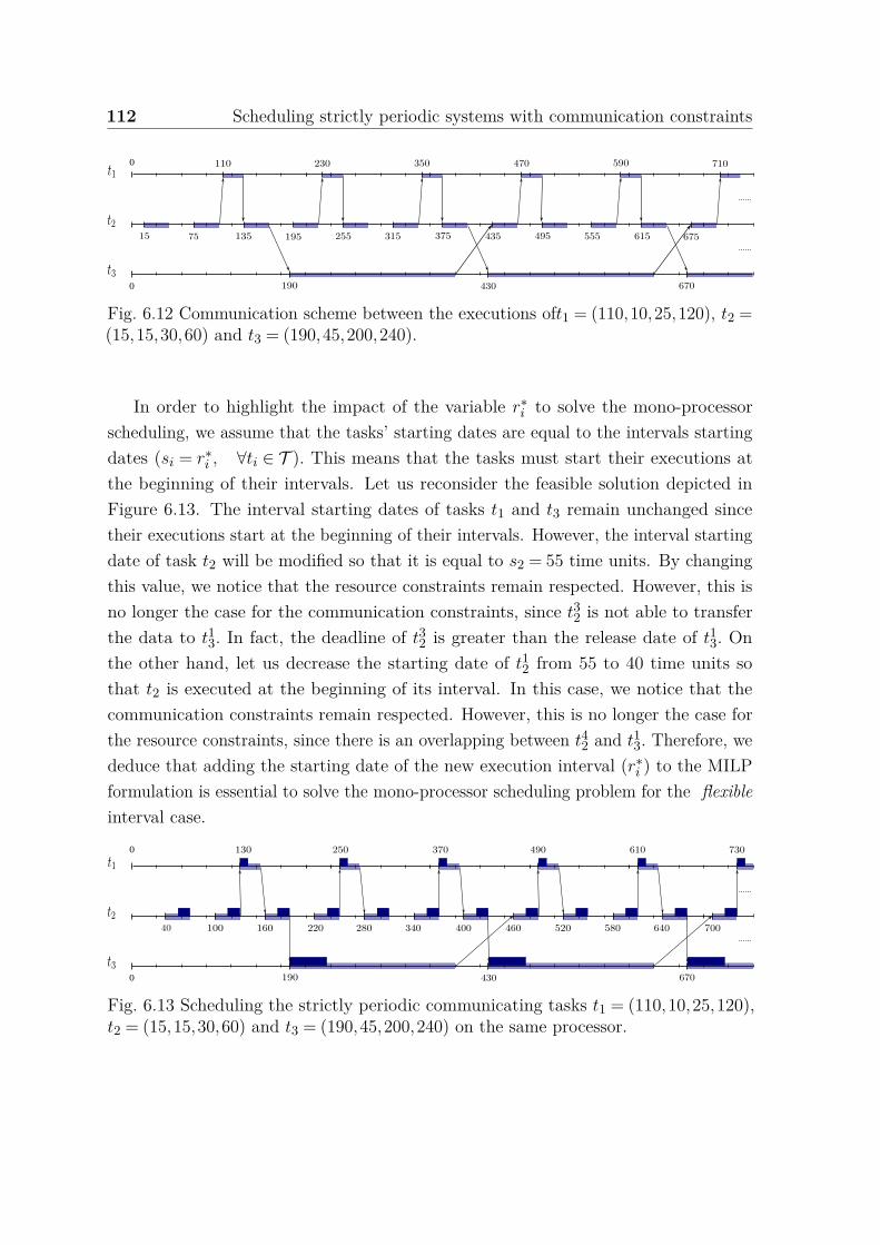
112 Scheduling strictly periodic systems with communication constraints
0
0
Fig. 6.12 Communication scheme between the executions oft1 = (110,10,25,120), t2 =(15,15,30,60) and t3 = (190,45,200,240).
In order to highlight the impact of the variable r∗i to solve the mono-processor
scheduling, we assume that the tasks’ starting dates are equal to the intervals startingdates (si = r∗
i , ∀ti ∈ T ). This means that the tasks must start their executions atthe beginning of their intervals. Let us reconsider the feasible solution depicted inFigure 6.13. The interval starting dates of tasks t1 and t3 remain unchanged sincetheir executions start at the beginning of their intervals. However, the interval startingdate of task t2 will be modified so that it is equal to s2 = 55 time units. By changingthis value, we notice that the resource constraints remain respected. However, this isno longer the case for the communication constraints, since t3
2 is not able to transferthe data to t1
3. In fact, the deadline of t32 is greater than the release date of t1
3. Onthe other hand, let us decrease the starting date of t1
2 from 55 to 40 time units sothat t2 is executed at the beginning of its interval. In this case, we notice that thecommunication constraints remain respected. However, this is no longer the case forthe resource constraints, since there is an overlapping between t4
2 and t13. Therefore, we
deduce that adding the starting date of the new execution interval (r∗i ) to the MILP
formulation is essential to solve the mono-processor scheduling problem for the flexibleinterval case.
0
0
Fig. 6.13 Scheduling the strictly periodic communicating tasks t1 = (110,10,25,120),t2 = (15,15,30,60) and t3 = (190,45,200,240) on the same processor.

6.5 Heuristics 113
6.5 HeuristicsSolving the MILP produces a schedule for a set of strictly periodic communicating taskson a single processor. Numerically solving the MILP within a reasonable amount oftime is only restricted to small instance. Recall that the scheduling problem in questionis known to be NP-complete in the strong sense [79]. Consequently, we present in thissection three heuristics which seek to find a feasible solution for our scheduling problem,such as linear programming relaxation. For the second and the third heuristic if nofeasible solution is found, a partial solution is computed. This solution corresponds toa subset of tasks that can be executed on the same processor.
6.5.1 Linear programming relaxation
Linear programming relaxation is a method which consists on transforming a com-binatorial or discrete problem to a continuous one. This method is used to obtaininformation on the initial discrete problem in order to build a solution. The linear pro-gramming relaxation may be solved using any standard linear programming technique(such as Simplex). Our first approach is based on the linear programming relaxationand it can be defined in the following steps:
• Relaxation of the integrality constrain: this relaxation allows variables to havenon-integral values. The MILP of the Flexible intervals case can be “ relaxed ”as follows :
subject tor∗
j − r∗i ≥Di +(Tj−M0(a)−gcda), ∀a = (ti, tj) ∈ A
r∗i ≥ ri, ∀ti ∈ T
r∗i ≤ si ≤ r∗
i +Di−Ci, ∀ti ∈ Tsj− si = δi,j +ki,j ·gi,j , ∀(ti, tj)
i<j∈ T 2
Ci ≤ δi,j ≤ gi,j−Cj , ∀(ti, tj)i<j
∈ T 2
(si, r∗i ) ∈ R2
+ ∀ti ∈ Tki,j ∈ R, δij ∈ R+ ∀(ti, tj)
i<j∈ T 2
• Solving the resulting linear program in order to obtain a fractional optimalsolution. We can notice that all the linear program constraints are potential
114 Scheduling strictly periodic systems with communication constraints
except the resource ones. For example, the precedence constraints induced bythe RTSDFG buffers are potential constraints, since the gap between the startingdate of the new execution intervals (r∗
j − r∗i ) are greater than or equal to an
integer constant. However, the equality sj− si = δi,j +ki,j ·gi,j is not potential.
• For each couple of tasks (ti, tj)i<j
∈ T 2, we compute the integer value of kij which
is equal to ⌊sj−si
gij⌋.
• We substitute each kij with its value in a new execution LP where kij is no longerconsidered as a variable. In order to verify the existence of a feasible (integer)solution to our scheduling problem, we solve the new LP. Note that finding afeasible solution for the new LP is equivalent to find a feasible solution for theoriginal MILP.
Let us reconsider the example depicted in figure 6.8. Fractional solution obtainedby solving the “ relaxed ” program is equal to:
s1 = 140 r∗1 = 120 k12 = 0.9167 δ12 = 10,
s2 = 260 r∗2 = 150 k13 =−0.8334 δ13 = 10,
s3 = 100 r∗3 = 90 k23 =−3.1667 δ23 = 30.
For each couple of tasks (ti, tj)i<j
∈ T 2, we compute the number of intervals of length gij
separating the starting dates of the tasks’ executions:
k12 = ⌊s2− s1g12
⌋= ⌊260−140120 ⌋= 1,
k13 = ⌊s3− s1g13
⌋= ⌊100−14060 ⌋=−1,
k23 = ⌊s3− s2g23
⌋= ⌊100−26060 ⌋=−3.
By solving the new LP where each kij is substituted by its integer value, we obtainthe following solution:
s1 = 90 r∗1 = 90 δ12 = 10,
s2 = 220 r∗2 = 150 δ13 = 40,
s3 = 70 r∗3 = 60 δ23 = 30.

6.5 Heuristics 115
0
900
Fig. 6.14 A feasible solution for the scheduling problem is obtained by solving the newLP with k12, k13 and k23 respectively equal to 1,−1 and −3.
Figure 6.14 illustrates the feasible solution obtained by solving the new LP. We noticethat there is no overlapping between the tasks executions and the communicationconstraints between them are fulfilled.
6.5.2 Simple heuristic
In this subsection, we describe in detail our simple heuristic for scheduling strictlyperiodic communicating tasks. It is based on the schedulability condition of two strictlyperiodic communicating tasks, which is presented previously in Section 6.3. In ourapproach, we use a greedy algorithm without back-tracking (i.e. if a decision is madeat some stage, it is never questioned during the following stages). The effectivenessof any greedy algorithm is predicated on the decisions choice. In the simple heuristic,decisions are based on two criteria: the interval length where each task can start itsexecution ([ri, ri +Di−Ci]) and the task period (Ti).
Our algorithm takes as input a sorted list of tasks (the sort description is representedsubsequently). In addition, this algorithm returns a feasible solution (if it is able tofind such a solution). Otherwise, it returns a partial solution that corresponds to asubset of tasks with their starting dates which can be executed on the same processor.
We sort the set of tasks in an ascending order according to the gap between thetasks relative deadlines and their execution times (Di−Ci). Moreover, if two taskshave the same gap between their deadlines and their execution times, the task withthe smallest period has a higher priority. In other words, the task with the smallestperiod is placed prior to the other task in the sorted list. More formally, we denote byLT the sorted list of tasks such that

116 Scheduling strictly periodic systems with communication constraints
LT = ti : ∀ti ∈ T , (Di−Ci)≤ (Di+1−Ci+1). If (Di−Ci) = (Di+1−Ci+1) thenthe task with the smallest period has a higher priority.
Algorithm 4 describes the simple heuristic as follows:
• First, we initialize an empty list Solution. We insert in this latter the first task ofLT while setting its starting date to its release date s1 = r1 (line 3). In addition,we remove this task from LT (line 4). Solution corresponds to the set of scheduledtasks in the partial or global scheduling.
• Then, we verify for each candidate task tj in LT if there exists a starting datesj ∈ [rj , rj +Dj−Cj ] which fulfils the schedulability condition with all tasks inthe current solution Solution. We run the test on the starting date values in anincreasing order (line 6). If such a starting date exists (line 7), we add the couple(tj , sj) to the current solution Solution (line 8). Even if this starting date does notexist, we continue to check the remaining tasks in LT in order to find a partialsolution and to compute the tasks percentage which can be executed on the sameprocessor.
• Finally, after checking all the tasks in LT , we return the current solution (line13). If |Solution|= n then Solution is a feasible solution. Otherwise, it is a partialsolution that contains the subset of tasks which can be scheduled on the sameprocessor.
Note that our algorithm always selects the first starting date value that satisfies theschedulability condition with current solution tasks. Changing the order of checkingthe tasks starting date values provides a new heuristic. For example, we can modifythe order in line 6 from an increasing order to a decreasing one.
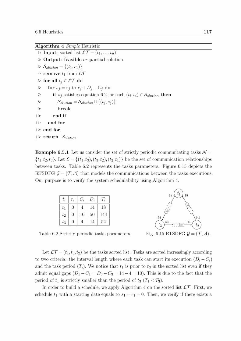
6.5 Heuristics 117
Algorithm 4 Simple Heuristic1: Input: sorted list LT = (t1, . . . , tn)2: Output: feasible or partial solution3: Solution = (t1, r1)4: remove t1 from LT5: for all tj ∈ LT do6: for sj = rj to rj +Dj−Cj do7: if sj satisfies equation 6.2 for each (ti, si) ∈ Solution then8: Solution = Solution∪(tj , sj)9: break
10: end if11: end for12: end for13: return Solution
Example 6.5.1 Let us consider the set of strictly periodic communicating tasks N =t1, t2, t3. Let E = (t1, t3),(t3, t2),(t2, t1) be the set of communication relationshipsbetween tasks. Table 6.2 represents the tasks parameters. Figure 6.15 depicts theRTSDFG G = (T ,A) that models the communications between the tasks executions.Our purpose is to verify the system schedulability using Algorithm 4.
ti ri Ci Di Ti
t1 0 4 14 18t2 0 10 50 144t3 0 4 14 54
Table 6.2 Strictly periodic tasks parameters Fig. 6.15 RTSDFG G = (T ,A).
Let LT = (t1, t3, t2) be the tasks sorted list. Tasks are sorted increasingly accordingto two criteria: the interval length where each task can start its execution (Di−Ci)and the task period (Ti). We notice that t1 is prior to t3 in the sorted list even if theyadmit equal gaps (D1−C1 = D3−C3 = 14−4 = 10). This is due to the fact that theperiod of t1 is strictly smaller than the period of t3 (T1 < T3).
In order to build a schedule, we apply Algorithm 4 on the sorted list LT . First, weschedule t1 with a starting date equals to s1 = r1 = 0. Then, we verify if there exists a

118 Scheduling strictly periodic systems with communication constraints
starting date s3 ∈ [0,10] that allows t3 to be executed on the same processor executingt1 (without overlapping). We run the test on the possible values of s3 in an increasingorder. Moreover, we select the first value that verify the schedulability condition with(t1, s1). In this example, s3 is equal to 4 time units. Using the same principle, we verifyif there is a starting date s2 ∈ [0,40] that allows t2 to be scheduled on the processorexecuting t1 and t3. t2 can be executed on this processor with a starting date equal to8 time units.
Figure 6.16 depicts the resulting scheduling using Algorithm 4. As we can see, thereis no overlapping between the tasks execution (i.e. resource constraints are fulfilled).In addition, we notice that communication constraints between the tasks executionsare satisfied, since each task starts its execution during the interval [ri, ri +Di−Ci].
0
Fig. 6.16 A feasible schedule of the strictly periodic system represented in Table 6.2and Figure 6.15. The tasks starting dates are respectively equal to s1 = 0, s2 = 8 ands3 = 4.
Partial solution
Let us modify the previous example by increasing the tasks release dates as follows:r1 = 10, r2 = 120 and r3 = 40 time units. In order to verify the system schedulabilityon a single processor, we apply Algorithm 4. Let LT = (t1, t3, t2) be the tasks sortedlist. First, we schedule t1 with a starting date equal to s1 = r1 = 10 time units. Then,we verify if there is a starting date value of s3 ∈ [40,50] that satisfies the schedulabilitycondition with the starting date of t1. In this case, s3 is equal to 40 time units. Finally,we check if there is a starting date s2 ∈ [120,160] that simultaneously satisfies theschedulability condition with t1 and t3. We release that such a date does not exist.More precisely, there is no starting date s2 ∈ [120,160] that verifies the schedulabilitycondition with (t3, s3). We can deduce that Algorithm 4 provides only a partial solution(see Figure 6.17) composed by the couples (t1,10) and (t3,40).

6.5 Heuristics 119
0
Fig. 6.17 A Partial solution of the scheduling problem using Algorithm 4. The tasksstarting dates are respectively equal to s1 = 10 and s3 = 40.
6.5.3 ACAP heuristic
In this part, we present the ACAP (As Close As Possible) heuristic which is also agreedy algorithm. As the the simple heuristic, our algorithm takes as input a sortedlist of tasks. These latter are sorted increasingly according to their gaps (Di−Ci)and their periods (Ti). In addition, this algorithm returns a feasible solution (if it isable to find such a solution). Otherwise, it returns a partial solution correspondingto a subset of tasks which can be executed on the same processor. In contrast to thesimple heuristic approach, a new priority is given to every candidate task in order to bescheduled with the current solution tasks. This priority depends on the candidate taskposition compared to the other tasks that are already scheduled. In fact, adding thispriority seeks to maximize the number of tasks that can executed on a single processorby scheduling the tasks as close as possible.
Scheduling two strictly periodic communicating tasks as close as possible
Let ti = (ri,Ci,Di,Ti) and tj = (rj ,Cj ,Dj ,Tj) be two strictly periodic communicatingtasks, such that ti is already scheduled on a processor with a staring date equal to si.
Let sj be the unknown starting date of tj . According to theorem 6.3.1, these taskscan be scheduled on the same processor if and only if equation (6.2) is fulfilled. Thisequation can be written as follows:
sj− si = δij +kij ·gij , (6.10)
where Ci ≤ δij ≤ gij−Cj and kij = ⌊sj−si
gij⌋.
In order to maximize the number of tasks that can be executed on the sameprocessor, we seek to schedule tj as close as possible to ti. Hence, we can distinguishtwo cases:
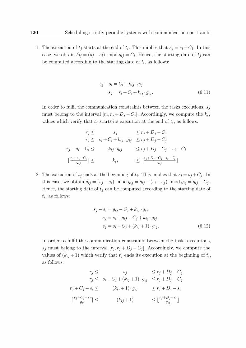
120 Scheduling strictly periodic systems with communication constraints
1. The execution of tj starts at the end of ti. This implies that sj = si +Ci. In thiscase, we obtain δij = (sj− si) mod gij = Ci. Hence, the starting date of tj canbe computed according to the starting date of ti, as follows:
sj− si = Ci +kij ·gij
sj = si +Ci +kij ·gij . (6.11)
In order to fulfil the communication constraints between the tasks executions, sj
must belong to the interval [rj , rj +Dj−Cj ]. Accordingly, we compute the kij
values which verify that tj starts its execution at the end of ti, as follows:
rj ≤ sj ≤ rj +Dj−Cj
rj ≤ si +Ci +kij ·gij ≤ rj +Dj−Cj
rj− si−Ci ≤ kij ·gij ≤ rj +Dj−Cj− si−Ci
⌈rj−si−Ci
gij⌉ ≤ kij ≤ ⌊rj+Dj−Cj−si−Ci
gij⌋
2. The execution of tj ends at the beginning of ti. This implies that si = sj +Cj . Inthis case, we obtain δij = (sj− si) mod gij = gij− (si− sj) mod gij = gij−Cj .
Hence, the starting date of tj can be computed according to the starting date ofti, as follows:
sj− si = gij−Cj +kij ·gij ,
sj = si +gij−Cj +kij ·gij ,
sj = si−Cj +(kij +1) ·gij , (6.12)
In order to fulfil the communication constraints between the tasks executions,sj must belong to the interval [rj , rj + Dj −Cj ]. Accordingly, we compute thevalues of (kij +1) which verify that tj ends its execution at the beginning of ti,as follows:
rj ≤ sj ≤ rj +Dj−Cj
rj ≤ si−Cj +(kij +1) ·gij ≤ rj +Dj−Cj
rj +Cj− si ≤ (kij +1) ·gij ≤ rj +Dj− si
⌈rj+Cj−si
gij⌉ ≤ (kij +1) ≤ ⌊rj+Dj−si
gij⌋

6.5 Heuristics 121
Let t1 = (10,4,14,18) and t2 = (120,10,50,144) be two strictly periodic communi-cating tasks. Let s1 and s2 be the tasks starting dates. we suppose that t1 is alreadyscheduled on a processor with a starting date s1 = 10. Hence, t2 can start its executionat the end of t1 if
s2 = s1 +C1 +kij ·gij
= 10+4+kij ·18,
with 6≤ kij ≤ 8. Figure 6.18 illustrates an example where task t2 begins its executionat the end of t1 with a starting date s2 = 14 + 6 · 18 = 122 time units. In addition,communication constraints are fulfilled since s2 ∈ [120,160].
0
Fig. 6.18 Scheduling task t2 = (120,10,50,144) at the end of the execution of taskt1 = (10,4,10,18) which is already scheduled with a starting date s1 = 10 time units.
On the other hand, t2 can end its execution at the beginning of t1 if
s2 = s1−C2 +(kij +1) ·gij
= 10−10+(kij +1) ·18,
with 7≤ (kij +1)≤ 8. Figure 6.19 illustrates an example where task t2 ends its executionat the beginning of t1 with a starting date s2 = 7 ·18 = 126 time units. In addition,communication constraints are fulfilled since s2 ∈ [120,160].
0
Fig. 6.19 Scheduling task t2 = (120,10,50,144) such that the end of its executioncorresponds to the beginning of task t1 = (10,4,10,18) which is already scheduled witha starting date s1 = 10 time units.

122 Scheduling strictly periodic systems with communication constraints
Our target is to maximize the number of tasks that can be scheduled on the sameprocessor. In order to achieve this goal, we seek to schedule each candidate task asclose as possible to the tasks that are already scheduled. Algorithm 5 describes indetails this approach as follows:
• As in the simple heuristic, we initialize an empty list Solution. We insert in thislatter the first task of LT while setting its starting date to its release date s1 = r1
(line 3). In addition, this task is removed from LT (line 4).
• Then, we initialize an empty list Slist (line 6). For each candidate task tj in LT ,
we verify if there exists a starting date sj ∈ [rj , rj + Dj −Cj ] which fulfils theschedulability condition with all tasks in the current solution Solution. We run thetest on the starting date values in an increasing order (line 8). If a given task tj
does not admit a starting date that satisfies the schedulability condition with allthe current solution tasks, then tj is removed from the list (line 11). In contrastwith the simple heuristic, we group in Slist all the couples (tj , sj) which verifythe schedulability condition with current solution tasks (line 14). Moreover, wegroup in S ′
list the couples from Slist which verify equation (6.11) or (6.12) withat least one couple (ti, si) ∈ Solution (line 20). In other words, we consider that acouple (tj , sj) ∈ S
′list has a higher priority, since its execution starts at the end
of a scheduled task. Moreover, this couple can also have a higher priority if itsexecution ends at the beginning of a scheduled task. Note that (tj , sj) ∈ S
′list
can verify both cases at the same time. This means that a candidate task canbegin at the end of a scheduled task and ends at the beginning of another one.
If several couples in S ′list have the same priority, we choose the couple with the
smallest gap (line 22). In addition, if S ′list is empty, we choose from Slist the
couple whose gap is minimal (line 24). We add the chosen couple (tj , sj) to thecurrent solution Solution and we remove tj from LT (lines 26 and 27). We repeatthe whole procedure as long as the list LT is not empty.
• Finally, once the tasks list LT is empty, we return the current solution (line30). If |Solution|= n then Solution is a feasible solution. Otherwise, it is a partialsolution that corresponds to a tasks subset and their starting dates, that can bescheduled on the same processor.
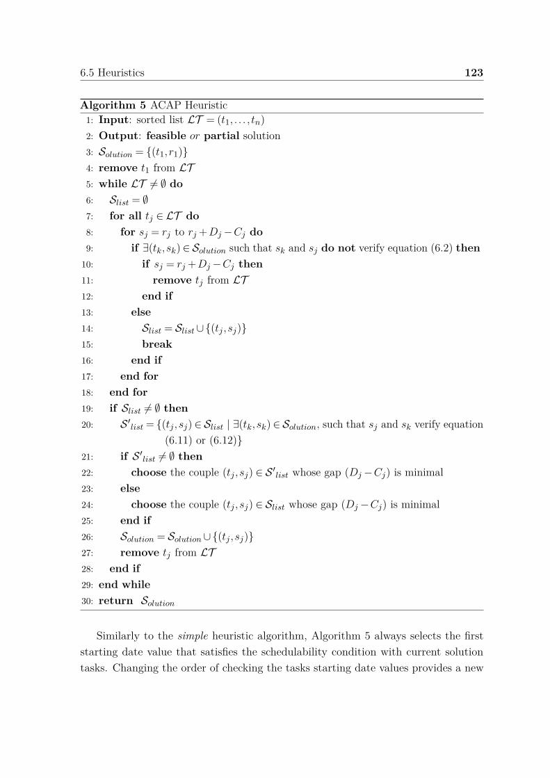
6.5 Heuristics 123
Algorithm 5 ACAP Heuristic1: Input: sorted list LT = (t1, . . . , tn)2: Output: feasible or partial solution3: Solution = (t1, r1)4: remove t1 from LT5: while LT = ∅ do6: Slist = ∅7: for all tj ∈ LT do8: for sj = rj to rj +Dj−Cj do9: if ∃(tk, sk)∈ Solution such that sk and sj do not verify equation (6.2) then
10: if sj = rj +Dj−Cj then11: remove tj from LT12: end if13: else14: Slist = Slist∪(tj , sj)15: break16: end if17: end for18: end for19: if Slist = ∅ then20: S ′
list = (tj , sj)∈ Slist | ∃(tk, sk)∈ Solution, such that sj and sk verify equation(6.11) or (6.12)
21: if S ′list = ∅ then
22: choose the couple (tj , sj) ∈ S ′list whose gap (Dj−Cj) is minimal
23: else24: choose the couple (tj , sj) ∈ Slist whose gap (Dj−Cj) is minimal25: end if26: Solution = Solution∪(tj , sj)27: remove tj from LT28: end if29: end while30: return Solution
Similarly to the simple heuristic algorithm, Algorithm 5 always selects the firststarting date value that satisfies the schedulability condition with current solutiontasks. Changing the order of checking the tasks starting date values provides a new

124 Scheduling strictly periodic systems with communication constraints
heuristic. This can be done by modifying the order in line 8 from an increasing orderto a decreasing one.
Example 6.5.2 Let us reconsider the system composed of three strictly periodiccommunicating tasks t1 = (10,4,14,18), t2 = (120,10,50,144) and t3 = (40,4,14,54).Recall that applying Algorithm 4 on this system provides only a partial solution. Inorder to verify the system schedulability on a single processor, we apply Algorithm5. Let LT = (t1, t3, t2) be the tasks sorted list. We schedule t1 with a starting dateequal to its release date s1 = r1 = 10 time units and we remove it from LT . Then,we compute for each task in LT its first starting date that fulfils the schedulabilitycondition with (t1,10). In this example, the tasks starting dates are respectively equalto s3 = 40 and s2 = 122 time units. We add the couples (t3,40) and (t2,122) to Slist.
Moreover, we check for each couple in Slist if its starting date satisfies equation (6.11)or (6.12) with s1 = 10 time units. We notice that s3 = 40 does not satisfy any equation.However, s2 = 122 verifies equation (6.11) with s1 = 10. This means that t2 starts itsexecution at the end of t1. Accordingly, t2 is given a higher priority and it is scheduledwith a starting date equal to s2 = 122 time units. Therefore, we remove t2 from LT .Finally, We check if there is a starting date s3 ∈ [40,50] that simultaneously verifies theschedulability condition with (t1,10) and (t2,122). We realize that t3 can be executedon the same processor with t1 and t2 with a starting date s3 = 42 time units.
0
Fig. 6.20 A feasible schedule resulting from applying Algorithm 5 on the perioidicsystem composed of t1 = (10,4,14,18), t2 = (120,10,50,144) and t3 = (40,4,14,54).The tasks starting dates are respectively equal to s1 = 10, s2 = 122 and s3 = 42 timeunits.
Figure 6.20 depicts the resulting schedule using Algorithm 5. As we can see, thetasks are scheduled as close as possible. For instance, the first execution of t3 endsat the beginning of the third execution of t1. On the other hand, the first executionof t2 starts at the end of the seventh execution of t1. In addition, we notice thatthe resource constraints are fulfilled, since there is no overlapping between the tasksexecutions. Moreover, communication constraints are fulfilled since each task ti starts

6.5 Heuristics 125
its execution during the interval [ri, ri + Di−Ci], such as s3 = 42 time units whichbelongs to [40,40+14−4].
Flexible interval case
In the flexible intervals case, the starting date of a task ti = (ri,Ci,Di,Ti) is nolonger restricted to the interval [ri, ri + Di−Ci]. Therefore, we need to know howwe might compute the starting date of the new execution interval (r∗
i ) knowingthat communication constraints between executions must always be respected. LetG = (T ,A) be a RTSDFG. For each task ti ∈ T , we denote by αi the length of therelease date interval to which the starting date of the new execution interval (r∗
i )belongs. More formally,
∀ti ∈ T , r∗i ∈ [ri, ri +αi].
Computing αi of a given task ti = (ri,Ci,Di,Ti) must respect the communicationconstraints between the executions of ti and that of its adjacent tasks. Accordingto our communication scheme of Section 5.1 in Chapter 5, the data consumptioncan only be done at the release date of the receiving task. As the starting date ofthe new execution interval (r∗
i ) is greater or equal to the task release date (ri), thecommunications constraints between the task and its predecessors are always fulfilled.Therefore, the αi computation depends only on the task’s release dates and those ofits successors. More precisely, it depends on the minimal latency separating the task’sexecutions and those of its successors. According to Theorem 5.2.2 in Section 5.2 ofChapter 5, the minimum latency between two periodic communicating tasks ti and tj ,such that ti is the emitting task and tj the receiving one, can be computed as follows:
Lmin(ti, tj) = rj− ri +λ−Di,
where λ = ⌈ri−rj+Di
gcda⌉ ·gcda and gcda = gcd(Ti,Tj).
Our approach computes the interval length αi of a task ti while taking into accountthat ti can admit successors that are already scheduled. Therefore, our algorithmtakes as input a candidate task ti = (ri,Ci,Di,Ti) and a current solution Solution =(tj , r
∗j , sj), such that tj is already scheduled. It returns the interval length (αi) to
which r∗i belongs.
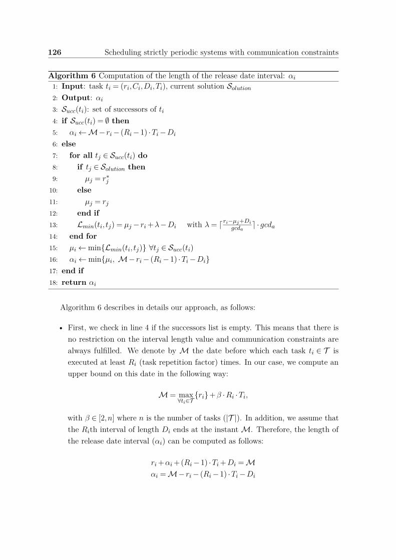
126 Scheduling strictly periodic systems with communication constraints
Algorithm 6 Computation of the length of the release date interval: αi
1: Input: task ti = (ri,Ci,Di,Ti), current solution Solution
2: Output: αi
3: Succ(ti): set of successors of ti
4: if Succ(ti) = ∅ then5: αi←M− ri− (Ri−1) ·Ti−Di
6: else7: for all tj ∈ Succ(ti) do8: if tj ∈ Solution then9: µj = r∗
j
10: else11: µj = rj
12: end if13: Lmin(ti, tj) = µj− ri +λ−Di with λ = ⌈ri−µj+Di
gcda⌉ ·gcda
14: end for15: µi←minLmin(ti, tj) ∀tj ∈ Succ(ti)16: αi←minµi, M− ri− (Ri−1) ·Ti−Di17: end if18: return αi
Algorithm 6 describes in details our approach, as follows:
• First, we check in line 4 if the successors list is empty. This means that there isno restriction on the interval length value and communication constraints arealways fulfilled. We denote by M the date before which each task ti ∈ T isexecuted at least Ri (task repetition factor) times. In our case, we compute anupper bound on this date in the following way:
M= max∀ti∈T
ri+β ·Ri ·Ti,
with β ∈ [2,n] where n is the number of tasks (|T |). In addition, we assume thatthe Rith interval of length Di ends at the instant M. Therefore, the length ofthe release date interval (αi) can be computed as follows:
ri +αi +(Ri−1) ·Ti +Di =Mαi =M− ri− (Ri−1) ·Ti−Di

6.5 Heuristics 127
• In contrast, if the successors list is not empty, lines 7 to 12 classify the successorstasks whether they are already scheduled or not. Accordingly, line 13 representsthe minimum latency computation between the task and its successor. In otherwords, we compute the minimum latency Lmin(ti, tj) according the starting dateof the new execution interval (r∗
i ) if the successor task is already scheduled.Otherwise, we compute this latency according to the successor release date. Inline 15, we compute µi which is equal to the minimum Lmin(ti, tj) between ti
and its successors. In line 16, we calculate the length of the release date interval(αi) by computing the minimum between µi and M− ri− (Ri−1) ·Ti−Di.
After computing the interval length αi, we compute the starting date of the newexecution interval r∗
i . Our approach consists of finding the task starting date si (ifit exists), and according to its value, we compute the interval starting date. Ouralgorithm takes as input a candidate task ti = (ri,Ci,Di,Ti), the length of its intervalrelease date αi and a current solution Solution. It returns the starting date of the newexecution interval (r∗
i ).
Algorithm 7 Computation of the starting date of the new execution interval: r∗i
1: Input: task ti = (ri,Ci,Di,Ti), current solution Solution, interval length αi
2: Output: r∗i
3: Prec(ti) : set of predecessors of ti
4: if ∃si ∈ [ri, ri +Di−Ci +αi] such that ti can be scheduled on the same processorwith the current solution tasks then
5: if ∃tj ∈ Prec(ti) such that tj /∈ Solution then6: r∗
i = min(ri +αi, si)7: else if si +Ci > ri +Di then8: r∗
i = si +Ci−Di
9: else10: r∗
i = ri
11: end if12: end if13: return r∗
i
Algorithm 7 computes the starting date of the new execution interval. First, line 3checks if there is a task starting date (si) which belongs to the interval [ri, ri +Di−Ci +αi], such that ti can be scheduled on the same processor with the current solutiontasks. We distinguish two cases:

128 Scheduling strictly periodic systems with communication constraints
1. Task ti admits a predecessor (tj ∈ Prec(ti)) which is not scheduled yet. If such apredecessor does exist (line 5), we seek to increase the starting date value of thenew execution interval (r∗
i ). This increases the possibility of finding a startingdate (sj) that allows the predecessor task (which is not scheduled yet) to beexecuted on the same processor with the current solution tasks. Therefore, r∗
i
can be computed (line 6) by finding the minimum between ri +αi and the taskstarting date si.
2. Task ti does not admit predecessors or admits predecessors that are alreadyscheduled. In this case, we check whether the task is partially or totally executedoutside the interval [ri, ri + Di]. If this occurs, the starting date of the newexecution interval is equal to si +Ci−Di (line 8). Otherwise, the task is totallyexecuted within the interval [ri, ri +Di] and r∗
i is equal to ri (line 10).
Our purpose is to solve the mono-processor scheduling problem for the flexibleintervals case using the simple or ACAP heuristics. In order to achieve our target, wemodify Algorithm 4 or 5 as follows:
• We verify whether the first task of the sorted list admits predecessors. If thisoccurs, we compute the length of the release date interval (αi) using Algorithm 6.Moreover, we schedule this task with a starting date si equal to ri +αi. Otherwise,we schedule this task with a starting date equals to its release date ri. In bothcases, the starting date of the new execution interval r∗
i is equal to the taskstarting date.
• After scheduling the first task, we seek to schedule the remaining tasks in LT .
Therefore, at the beginning of each iteration of Algorithm 4, we compute forthe candidate task the length of its release date interval (αi) (using Algorithm6). However, at the beginning of each iteration of Algorithm 5, we compute forevery remaining task in LT the length of its release date interval (αi) (usingAlgorithm 6). In both cases, we need to find the first date which allows thetask to be scheduled on the same processor with the current solution tasks.In order to do that, we run the test on the starting date value in the interval[ri, ri +Di−Ci +αi].
• Once the task’s starting date si is fixed, we compute its starting date of the newexecution interval r∗
i according to si using Algorithm 7.
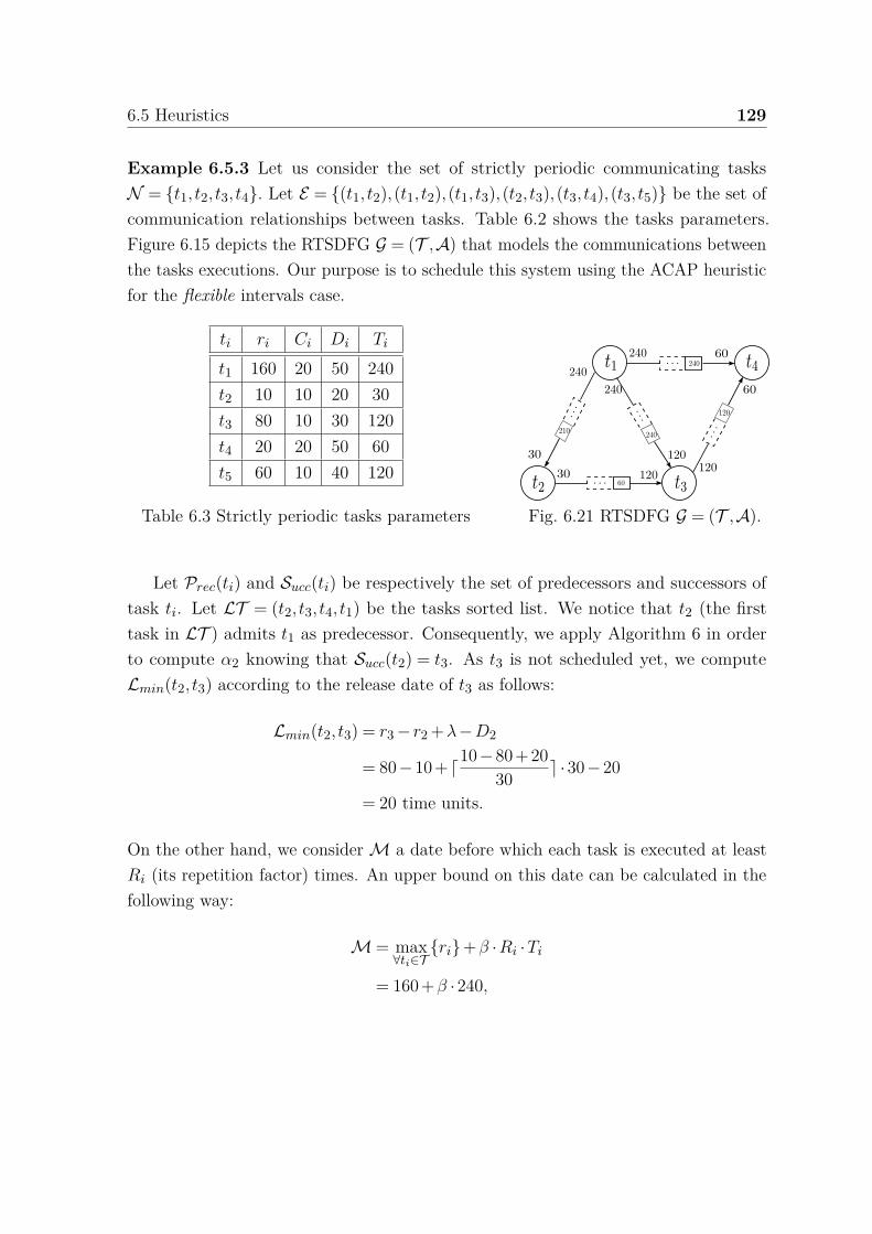
6.5 Heuristics 129
Example 6.5.3 Let us consider the set of strictly periodic communicating tasksN = t1, t2, t3, t4. Let E = (t1, t2),(t1, t2),(t1, t3),(t2, t3),(t3, t4),(t3, t5) be the set ofcommunication relationships between tasks. Table 6.2 shows the tasks parameters.Figure 6.15 depicts the RTSDFG G = (T ,A) that models the communications betweenthe tasks executions. Our purpose is to schedule this system using the ACAP heuristicfor the flexible intervals case.
ti ri Ci Di Ti
t1 160 20 50 240t2 10 10 20 30t3 80 10 30 120t4 20 20 50 60t5 60 10 40 120
Table 6.3 Strictly periodic tasks parameters Fig. 6.21 RTSDFG G = (T ,A).
Let Prec(ti) and Succ(ti) be respectively the set of predecessors and successors oftask ti. Let LT = (t2, t3, t4, t1) be the tasks sorted list. We notice that t2 (the firsttask in LT ) admits t1 as predecessor. Consequently, we apply Algorithm 6 in orderto compute α2 knowing that Succ(t2) = t3. As t3 is not scheduled yet, we computeLmin(t2, t3) according to the release date of t3 as follows:
Lmin(t2, t3) = r3− r2 +λ−D2
= 80−10+ ⌈10−80+2030 ⌉ ·30−20
= 20 time units.
On the other hand, we consider M a date before which each task is executed at leastRi (its repetition factor) times. An upper bound on this date can be calculated in thefollowing way:
M= max∀ti∈T
ri+β ·Ri ·Ti
= 160+β ·240,

130 Scheduling strictly periodic systems with communication constraints
with β ∈ [2,4]. In this example, we consider β = 4. Hence, the length of the releasedate interval is equal to
α2 = minLmin(t2, t3),M− r2− (R2−1) ·T2−D2= min20,1120−10− (8−1) ·30−30= min20,870= 20 time units.
Once α2 computed, we schedule t2 with a starting date of the new execution intervalequals to
s2 = r∗2 = r2 +α2 = 10+20 = 30 time units.
We add (t2,30,30) to the current solution Solution and we remove t2 from LT . At thebeginning of the first iteration, we apply Algorithm 6 on each task in LT = (t3, t4, t1).The computed values of αi are α3 = 30, α4 = 870 and α1 = 0 time units. Hence, s3,s4 and s1 are tested in the intervals [80,130], [20,920] and [160,190], respectively. Wecompute for each task its first starting date that fulfils the schedulability conditionwith (t2,30,30). In this iteration, these dates are respectively equal to s3 = 80, s4 = 40and s1 = 160 time units. Moreover, we verify for every task if its starting date satisfiesequation (6.11) or (6.12) with s2 = 30 time units. We notice that s3 = 80 verifiesequation (6.12). However, s4 = 40 and s1 = 160 fulfil both equations at the sametime. This means that t4 and t1 can be exactly executed between two successiveexecutions of t2. More specifically, their starting dates (s4 and s1) coincide with theend date of an execution of t2 and their end dates (s4 + C4 and s1 + C1) coincide withthe starting date of the next execution of t2. In addition, t4 has a smaller gap than t1
(D4−C4 < D1−C1). Accordingly, t4 is given a higher priority and it is scheduled withs4 = 40 time units. After computing s4, we apply Algorithm 7 in order to calculate thestarting date of the new execution interval r∗
4. As t4 admits t1 and t3 as predecessors(which are not scheduled yet), r∗
4 can be computed as follows:
r∗4 = min(r4 +α4, s4)
= min(20+870,40)= 40 time units.
This procedure is repeated as long as the list LT is not empty. At the second iteration,we schedule t1 with s1 = 190 and r∗
1 = 160 time units (since Prec(t1) = ∅ and the task istotally executed in the interval [160,210]). Finally, we schedule t3 with s3 = 130 time

6.6 Conclusion 131
units. As t3 is executed outside the interval [80,110] and all its predecessor are alreadyscheduled, r∗
3 is equal to s3 +C3−D3 = 130+10−30 = 110 time units.Figure 6.22 illustrates the feasible schedule resulting from applying Algorithm 5
for the flexible case. The tasks’ starting dates are s1 = 190, s2 = 30, s3 = 130 ands4 = 40 time units. The starting dates of the new execution intervals are r∗
1 = 160,r∗
2 = 30, r∗3 = 110 and r∗
4 = 40 time units. We notice that the resource constraintsare fulfilled since there is no overlapping between the tasks executions. Moreover,communication constraints are fulfilled since each task ti starts its execution during theinterval [r∗
i , r∗i +Di−Ci], such as s4 = 40 time units which belongs to [40,40+90−20].
0
Fig. 6.22 A feasible schedule of the strictly periodic system represented in Table 6.3and Figure 6.21. The tasks starting dates are s1 = 190, s2 = 30, s3 = 130 and s4 = 40time units. In addition, the starting dates of the new execution intervals are r∗
1 = 160,r∗
2 = 30, r∗3 = 110 and r∗
4 = 40 time units.
6.6 ConclusionThis chapter has introduced an overview of strictly periodic tasks and their charac-teristics. According to the communication model defined in Chapter 5, we provedthat scheduling two periodic communicating tasks is equivalent to schedule two in-dependent tasks. These latter can only be executed between their release dates andtheir deadlines. In order to solve the mono-processor scheduling problem of a strictlyperiodic communicating system, we propose an optimal (exact) algorithm using MILPformulations. Two cases were treated: the fixed and flexible interval cases. In thefixed case, tasks execution is only restricted to the interval beginning at its releasedate and ending at its deadline. However, in the flexible case, tasks can admit newexecution intervals whose lengths are equal to their relative deadlines. The schedulingproblem is know to be NP-complete in strong sense [79]. This means, obtaining feasibleschedule is practicable only for small instances. In order to solve this issue, we proposedthree heuristics: linear programming relaxation, simple and ACAP heuristics. For
132 Scheduling strictly periodic systems with communication constraints
the second and the third heuristic if no feasible solution is found, a partial solution iscomputed. This solution corresponds to a subset of tasks that can be executed on thesame processor.
The next chapter presents the experimental results of this thesis. It is devotedto evaluating the methods that compute the worst case system latency using theRTSDFG formalism. In addition, it presents several experiments dedicated to evaluatethe performance of our methods that solve the mono-processor scheduling problem.

Chapter 7
Experimental Results
This chapter presents the experimental results of this thesis. Section 7.1 present brieflythe random generator used to generate our RTSDFGs instances. Section 7.2 is devotedto evaluate our methods that compute the worst case latency of a RTSDFG. Section 7.3evaluates the performance of our algorithms that solve the mono-processor schedulingproblem of strictly periodic communicating systems. Section 7.4 concludes the chapter.
7.1 Graph generation: TurbineBodin et al.[19] recently developed a data flow random generator “Turbine”. It generatesrandomly a Phased Computation Graph (PCG in short) [116] which is an extension ofthe SDFG model. Turbine requires several parameters to be fixed in order to generateinstances. Some of these parameters are directly related to the graph structure, suchas the total number of tasks |T | and their degrees. The other parameters, as theaverage value of the repetition vector
(RT =
∑t∈T Rt
|T |
), control the random generation
of production and consumption rates.Turbine is implemented using Python and the graph library NetworkX that manage
the graph data structure. Random generation is composed of three steps. The firststep generates a random graph with nodes and arcs. The second step computes theconsumption and production rates of the graph. The last step computes a live initialmarking using the Linear Programming Solver (GLPK).
In our study, we added to Turbine two parameters: the task release date (ri) andits relative deadline (Di). The initial marking of each buffer a = (ti, tj) is computed asfollows:
M0(a) = Tj +λ−gcda,
134 Experimental Results
where λ = ⌈ri−rj+Di
gcda⌉ ·gcda and gcda = gcd(Ti,Tj). The relative deadline was generated
randomly such that its value do not exceed the production (or consumption) rate. Theduration of each task was generated randomly in such way that it does not exceed thetask relative deadline.
7.2 Latency evaluationThis section is devoted to evaluate our methods that compute the worst case latencyof a RTSDFG. We expose different results for the exact evaluation, upper and lowerbounds. These results are obtained by modifying several parameters such as the averagerepetition factor and the number of tasks. Finally, we verify the quality of our boundsand the complexity of our algorithms.
We generated randomly acyclic RTSDFG instances. The buffer production andconsumption rates were chosen uniformly from the following set
F = Ti :R> 0, R≡ 0 mod Ti,
where R is a fixed strictly positive integer and F the set of its divisors. In addition,the tasks’ release dates were randomly generated from the set 0, . . . , lcm with lcm =lcm
∀ti∈T(Ti).
Complexity
The transformation from a RTSDFG to an equivalent graph G ′ , which presents allthe precedence and dependence constraints between the tasks executions, uses amathematical equation of complexity O(RT ) where RT is the average repetition factorof the tasks. However, transforming a RTSDFG into an weighted graph Gmax (or Gmin),which represents the required time to transfer the data in the worst (or best) casescenario, uses mathematical equation of complexity O(1). Furthermore, the differentevaluation processes of the worst case latency use the same algorithm that computesthe length of the longest path in a DAG. Its complexity is O(|T |+ |A|). Therefore,complexity of the latency exact evaluation is O(RT · (|T |+ |A|)), while the complexityof computing its bounds is O(|T |+ |A|).

7.2 Latency evaluation 135
7.2.1 Computation time
The experiments were performed on a Intel(R) Core2Duo [email protected] using 2 GBof RAM. We set up parallel calculations for some instances on a server with 48 cores.Each algorithm was launched on 100 instances. Each one returned the average valueof the exact latency evaluation, upper and lower bound as well as their computationtimes. Four graphs sizes have been chosen: Small for 100 tasks, Medium for 500 tasks,Large for 1000 tasks and Huge for 10000 tasks. Input and output degrees of a taskbelong to the set 1,2,3,4,5.
RTComputation time (s)
Exact evaluation Upper bound Lower bound5 22.23 5.24 4.9325 107.14 5.20 5.1245 212.71 5.22 5.0575 337.72 5.23 4.98125 557.25 5.32 5.11
Table 7.1 Average computation time of latency evaluation methods for Huge RTSDFGswith respect to their average repetition factors.
In Table 7.1, the size of the RTSDFG is fixed to 10000 tasks. Average repetitionfactors were varied in order to present the latency computation time for the exactevaluation, upper and lower bounds. By increasing the average repetition factor ofthe tasks, the time required to compute the exact value of the worst-case latencyincreases (linearly). Contrariwise, the time needed to compute the bounds remainsapproximately constant (equal to 5 seconds).
|T | Computation time (s)Exact evaluation Upper bound Lower bound
Small 3.40 0.15 0.15Medium 16.76 0.46 0.45Large 34.11 0.93 0.93Huge 337.72 5.23 4.98
Table 7.2 Average computation time of latency evaluation methods for RTSDFGsaccording to their size |T |. The average repetition factor is fixed to 75.
Through varying the sizes of RTSDFGs, table 7.2 and 7.3 present a comparisonbetween the average computation times of an exact value and its bounds. The averagerepetition factors were fixed to 75 and 750 respectively. In both cases, the average time

136 Experimental Results
|T | Computation time (s)Exact evaluation Upper bound Lower bound
Small 37.58 0.23 0.23Medium 196.43 0.62 0.61Large 481.52 0.97 0.97Huge 3898.26 5.04 5.62
Table 7.3 Average computation time of latency evaluation methods for RTSDFGsaccording to their size |T |. The average repetition factor is fixed to 750.
required to compute the latency bounds remains reasonable (in the range of seconds)compared to that of the exact value. For instance, computing the worst case latencyexact value of a Huge graph with a average repetition factor is 750, requires on averagemore than one hour. However, the computing its lower and upper bounds requiresapproximately 5 seconds.
7.2.2 Quality of bounds
0
1000
2000
3000
4000
5000
6000
7000
Small Medium Large Huge
Late
ncy
(Tim
e U
nit
s)
RTSDFG size (|T|)
Upper boundExact evaluation
Lower bound
Fig. 7.1 Average latency value using the evaluation methods with respect to the graphsize |T |.The average repetition was fixed to 125.
The histogram in Figure 7.1 represents the latency evaluations with respect tothe graph size. The average repetition factor was fixed to 125. The analysis of theseresults shows that the gap between the exact evaluation and its upper bound on one

7.2 Latency evaluation 137
hand is smaller than the gap between the same exact value and its lower bound onthe other hand. This is due to the fact that the exact value and the upper bound areboth computed in the worst case scenario, whereas, the lower bound is computed inthe best case scenario.
In this experiment, we evaluated the impact of the average repetition factor (RT )on evaluating the worst case system latency. Therefore, we generated acyclic RTSDFGwithout release dates (∀ti ∈ T , ri = 0).
0
5
10
15
20
25
Small Medium Large Huge
Devia
tion r
ati
o (
%)
RTSDFG size (|T|)
Average repetition factor = 5Average repetition factor = 25Average repetition factor = 45
(a) Upper bound.
0
5
10
15
20
25
30
35
Small Medium Large Huge
Devia
tion r
ati
o (
%)
RTSDFG size (|T|)
Average repetition factor = 5Average repetition factor = 25Average repetition factor = 45
(b) Lower bound.
Fig. 7.2 Deviation ratio between the latency exact value and its bounds. Deviationratio of upper bound is equal to drup = upper−exact
exact ×100%. Deviation ratio of lowerbound is equal to drlw = exact−lower
exact ×100%.
Deviation ratio is the percentage of gaps between the latency exact value andits bounds. We denote by drup as the deviation ratio of the upper bound which is
138 Experimental Results
computed as follows:drup = upper− exact
exact ×100%.
However, we denote by drlw as the deviation ratio of the lower bound which is computedas follows:
drlw = exact− lowerexact ×100%.
Through varying the average repetition factor for different size of RTSDFGs, thehistograms in Figure 7.2a and 7.2b depict the deviation ratios of the latency upper andlower bounds respectively. For different size of RTSDFGs, we notice that deviationratios increase with the average repetition factors. This is due to the time requiredto transfer the data between two communicating tasks in the worst (or best) casescenario. The computation of this duration is strongly dependant from the production(or consumption) rates whose generation is tightly related to the average repetitionfactor. In addition, we can deduce that the deviation ratio between the exact value andthe upper bound ranges between 10 and 15 %. However, the deviation ratio betweenthe exact value and the lower bound varies between 20 and 30 %.
7.3 Mono-processor schedulingAn important challenge is solving scheduling problems of complex real-time systems.These problems can lead to large-scale mathematical formulations which are intractable,even with modern optimization solvers. In other words, there are many schedulingproblems that cannot easily be solved, even with commercial mixed-integer program-ming software packages such as Gurobi Optimizer.
This section presents several experiments dedicated to evaluate the performanceof our methods that solve the mono-processor scheduling problem of strictly periodiccommunicating systems. First, we describe the generation of the task parameters.Then, we expose several results concerning the resolution of the scheduling problemwith an exact algorithm for different types of instances. Finally, we present the resultsobtained by applying our heuristics on the same instances.
7.3.1 Generation of tasks parameters
Using the modified version of Turbine, we generated cyclic and acyclic instances ofRTSDFGs. Parameters of each task have been generated as follows:

7.3 Mono-processor scheduling 139
• Task utilization factors (ui, 1≤ i≤ n) have been generated based using UUnifastalgorithm [18]. The complexity of this algorithm is O(n) and the generatedutilization factors are characterized by a uniform distribution.
• Harmonic tasks periods, i.e. each period is multiple of all other periods with lesservalue, were uniformly chosen form the set Ti : Ti+1 = k ·Ti with the period ratiok ∈ 2,3,4,5. The value of the first period (T1) was equal to 500. However, non-harmonic periods were chosen uniformly from the set 2x ·3y ·50 : x,y ∈ [0,4]2,which is inspired from [38]. In both cases, the size of the set containing theperiods values was fixed to 5.
• Task worst case execution time was computed according to the task period andits utilisation factor, as follows: Ci = ⌈Ti ·ui⌉.
• Task relative deadline was generated randomly such that its value is greater orequal to the task execution time on one hand, and its lesser or equal to the taskperiod on the other hand (Ci ≤Di ≤ Ti).
• Task release date was generated randomly from the set 0, . . . , lcm where lcm =lcm
i∈1,...,n(Ti).
ti 1 2 3 4 5 6 7 8 9 10Ti 7200 2700 2700 600 7200 150 150 900 150 2700Ci 690 198 216 36 210 6 12 54 12 6ri 4367 20989 19680 6240 5696 12841 5347 13844 10472 9059Di 3876 1154 2254 412 5847 33 32 588 115 1345
Table 7.4 Example of 10 non-harmonic tasks. Each task is characterized by a periodTi, worst case execution time Ci, release date ri and relative deadline Di. The lcmbetween the task periods is equal to 21600.
Table 7.4 presents an example of a non-harmonic instance temporal parameters.The graph size was equal to 10 tasks and the system utilization was 0.6.
7.3.2 Optimal algorithm
In this subsection, we present some experimental results to evaluate the performance ofour exact algorithms for both fixed and flexible cases. The MILP formulations for themono-processor scheduling problem are solved using the mixed-integer programmingsolver Gurobi (Academic license - for non-commercial use only).
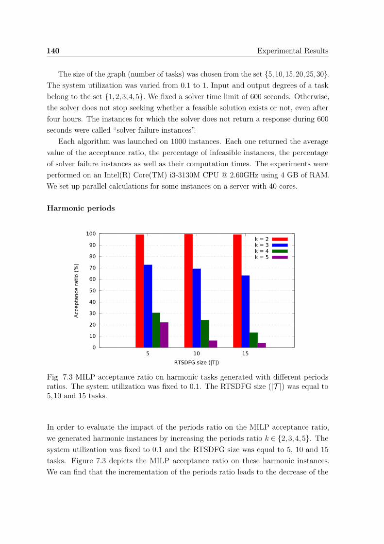
140 Experimental Results
The size of the graph (number of tasks) was chosen from the set 5,10,15,20,25,30.The system utilization was varied from 0.1 to 1. Input and output degrees of a taskbelong to the set 1,2,3,4,5. We fixed a solver time limit of 600 seconds. Otherwise,the solver does not stop seeking whether a feasible solution exists or not, even afterfour hours. The instances for which the solver does not return a response during 600seconds were called “solver failure instances”.
Each algorithm was launched on 1000 instances. Each one returned the averagevalue of the acceptance ratio, the percentage of infeasible instances, the percentageof solver failure instances as well as their computation times. The experiments wereperformed on an Intel(R) Core(TM) i3-3130M CPU @ 2.60GHz using 4 GB of RAM.We set up parallel calculations for some instances on a server with 40 cores.
Harmonic periods
0
10
20
30
40
50
60
70
80
90
100
5 10 15
Acc
epta
nce
rati
o (
%)
RTSDFG size (|T|)
k = 2k = 3k = 4k = 5
Fig. 7.3 MILP acceptance ratio on harmonic tasks generated with different periodsratios. The system utilization was fixed to 0.1. The RTSDFG size (|T |) was equal to5,10 and 15 tasks.
In order to evaluate the impact of the periods ratio on the MILP acceptance ratio,we generated harmonic instances by increasing the periods ratio k ∈ 2,3,4,5. Thesystem utilization was fixed to 0.1 and the RTSDFG size was equal to 5, 10 and 15tasks. Figure 7.3 depicts the MILP acceptance ratio on these harmonic instances.We can find that the incrementation of the periods ratio leads to the decrease of the

7.3 Mono-processor scheduling 141
MILP acceptance ratio. For example, when the RTSDFG size is equal to 10 tasks, theacceptance ratio decreases from 99.6% for k = 2 to 6.1% for k = 5. In fact, the increaseof the period ratio induces an increase in the period values as well as an increase in thegap between the period values. In addition, this increase in the periods values leadsto larger worst execution times (Ci = ⌈Ti ·ui⌉). For these reasons, finding a feasibleschedule is more and more difficult. Therefore, the MILP acceptance ratio decreasesby increasing the periods ratio.
In the sequel, harmonic instances were generated with a period ratio equals to 2.
The histogram in Figure 7.4a represents the MILP acceptance ratio with respectto the RTSDFG size (number of tasks) and the system utilization. For a systemutilization between 0.3 and 0.6, we notice that the MILP acceptance ratio increaseswith increasing size of RTSDFG. In fact, the increase in the number of tasks leads to areduction in the tasks worst case execution times. This allows to find more feasibleschedules. However, this is no longer the case once the system utilization is equal to0.8. For example, the acceptance ratio decreases from 15.3% for |T |= 10 to 8.9% for|T |= 15.This is due to the tasks worst case execution times for |T |= 15 which are notsmall enough to be scheduled on the same processor.
For a fixed size of RTSDFG, we notice that the acceptance ratio decreases with theincrease of the system utilization. For instance, when the RTSDFG size is equal to20 tasks, the acceptance ratio decreases from 88.8% for U = 0.3 to 17.5% for U = 0.8.Indeed, the tasks worst execution times grow with the increase of the system utilization.
Figure 7.4b demonstrates that the average computation time to find a feasible solu-tion increases with the incrementation of the RTSDFG size and the system utilization.For example, when the system utilization is 0.7, the time required to find a feasiblesolution increases from 0.92 seconds for |T |= 10 to 130.68 seconds for |T |= 25. This isdue to the number of the MILP variables that grows with the increase of the RTSDFGsize. Moreover, when the RTSDFG size is equal to 20 tasks, the time required to find afeasible solution increases from 1.08 seconds for U = 0.4 to 40.46 seconds for U = 0.8.
This means that the increase in the worst execution time (due to the system utilizationincrement) requires the solver to use a larger amount of time in order to find a feasiblesolution.

142 Experimental Results
0
10
20
30
40
50
60
70
80
90
100
0.3 0.4 0.5 0.6 0.7 0.8
Acc
ep
tance
rati
o (
%)
System utilization (U)
|T| = 10|T| = 15|T| = 20|T| = 25
(a) MILP acceptance ratio (%).
0.1
1
10
100
1000
0.1 0.2 0.3 0.4 0.5 0.6 0.7 0.8
Com
puta
tion t
ime (
s)
system utilization (U)
|T| = 10|T| = 15|T| = 20|T| = 25
(b) Average computation time to find a feasible schedule.
Fig. 7.4 Experimental results on harmonic instances of RTSDFGs with differentRTSDFG sizes (|T |) and system utilizations (U).
Harmonic versus Non Harmonic periods
In order to evaluate the effects of the tasks periods on our exact method, we generatedharmonic and non-harmonic instances with different system utilizations. The RTSDFGsize was fixed to 20 tasks. Figure 7.5a presents a comparison between the MILPacceptance ratio for harmonic and non-harmonic instances with respect to the systemutilization. We notice that the acceptance ratio on harmonic instances is greater thanthat on non-harmonic ones. For example, when the system utilization is 0.3, the
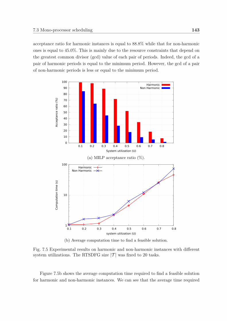
7.3 Mono-processor scheduling 143
acceptance ratio for harmonic instances is equal to 88.8% while that for non-harmonicones is equal to 45.0%. This is mainly due to the resource constraints that depend onthe greatest common divisor (gcd) value of each pair of periods. Indeed, the gcd of apair of harmonic periods is equal to the minimum period. However, the gcd of a pairof non-harmonic periods is less or equal to the minimum period.
0
10
20
30
40
50
60
70
80
90
100
0.1 0.2 0.3 0.4 0.5 0.6 0.7 0.8
Acc
ep
tance
rati
o (
%)
System utilization (U)
HarmonicNon Harmonic
(a) MILP acceptance ratio (%).
1
10
100
0.1 0.2 0.3 0.4 0.5 0.6 0.7 0.8
Com
puta
tion t
ime (
s)
system utilization (U)
HarmonicNon Harmonic
(b) Average computation time to find a feasible solution.
Fig. 7.5 Experimental results on harmonic and non-harmonic instances with differentsystem utilizations. The RTSDFG size |T | was fixed to 20 tasks.
Figure 7.5b shows the average computation time required to find a feasible solutionfor harmonic and non-harmonic instances. We can see that the average time required
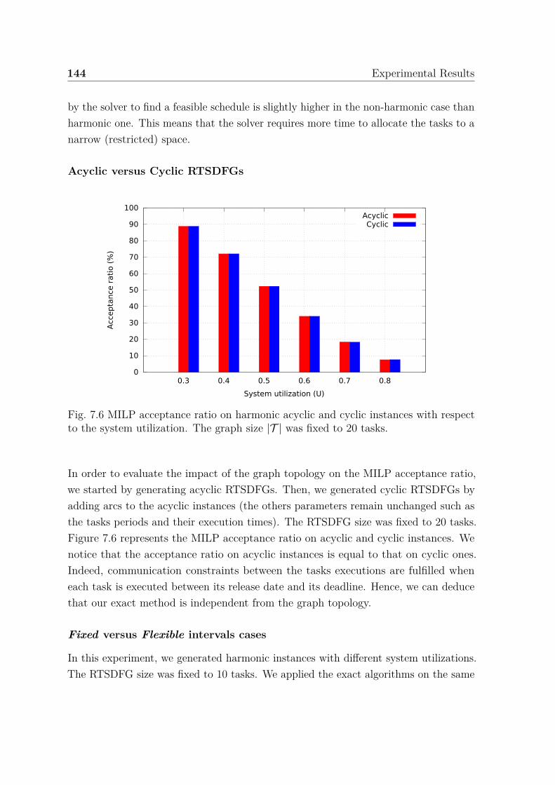
144 Experimental Results
by the solver to find a feasible schedule is slightly higher in the non-harmonic case thanharmonic one. This means that the solver requires more time to allocate the tasks to anarrow (restricted) space.
Acyclic versus Cyclic RTSDFGs
0
10
20
30
40
50
60
70
80
90
100
0.3 0.4 0.5 0.6 0.7 0.8
Acc
epta
nce
rati
o (
%)
System utilization (U)
AcyclicCyclic
Fig. 7.6 MILP acceptance ratio on harmonic acyclic and cyclic instances with respectto the system utilization. The graph size |T | was fixed to 20 tasks.
In order to evaluate the impact of the graph topology on the MILP acceptance ratio,we started by generating acyclic RTSDFGs. Then, we generated cyclic RTSDFGs byadding arcs to the acyclic instances (the others parameters remain unchanged such asthe tasks periods and their execution times). The RTSDFG size was fixed to 20 tasks.Figure 7.6 represents the MILP acceptance ratio on acyclic and cyclic instances. Wenotice that the acceptance ratio on acyclic instances is equal to that on cyclic ones.Indeed, communication constraints between the tasks executions are fulfilled wheneach task is executed between its release date and its deadline. Hence, we can deducethat our exact method is independent from the graph topology.
Fixed versus Flexible intervals cases
In this experiment, we generated harmonic instances with different system utilizations.The RTSDFG size was fixed to 10 tasks. We applied the exact algorithms on the same

7.3 Mono-processor scheduling 145
instances for both fixed and flexible cases. Figure 7.7a presents the MILP acceptanceratio for both cases. We notice that the acceptance ratio for the flexible case is higherthan the fixed one. The gap between these ratios varies between 2% and 7%. In fact,scheduling a task in the flexible case is no longer restricted to the interval between itsrelease date and its deadline as in the fixed case. This allows the solver to find morefeasible solutions in the flexible case than the the fixed one.
0
10
20
30
40
50
60
70
80
90
100
0.1 0.2 0.3 0.4 0.5 0.6 0.7 0.8 0.9
Acc
ep
tance
rati
o (
%)
System utilization (U)
flexiblefixed
(a) MILP acceptance ratio for fixed and flexible cases with respect tothe system utilization.
0.1
1
10
100
0.1 0.2 0.3 0.4 0.5 0.6 0.7 0.8 0.9
Com
puta
tion t
ime (
s)
system utilization (U)
flexiblefixed
(b) Average computation time to find a feasible solution in fixed andflexible cases.
Fig. 7.7 Experimental results on harmonic instances for fixed and flexible cases. TheRTSDFG size |T | was fixed to 10 tasks.

146 Experimental Results
Figure 7.7b shows the average computation time to find a feasible schedule in bothflexible and fixed cases. We notice that the time required by the solver to find a feasiblesolution in the flexible case is higher than in the fixed one. For example, when thesystem utilization is 0.8, the solver requires on average 1.04 seconds to find a feasibleschedule in the fixed case while it requires 44.48 seconds in the flexible case. This isdue to the addition of the interval starting date (r∗
i ) variable in the flexible case.
0
5
10
15
20
25
30
35
0.3 0.4 0.5 0.6 0.7 0.8 0.9 1
Solv
er
failu
re inst
ance
s (%
)
System utilization (U)
flexiblefixed
Fig. 7.8 Percentage of solver failure instances for fixed and flexible cases with respectto the system utilization. The RTSDFG size |T | was fixed to 20 tasks.
As we mentioned before, the solver time limit was fixed 600 seconds. Figure 7.8presents a comparison between the percentage of solver failure instances for the flexibleand fixed cases. The RTSDFG size was fixed to 20 tasks. We can see that the percentageof solver failure instances in the flexible case is considerably higher than in the fixedcase. This is due to the combinatorial explosion generated by the addition of variablesin the flexible case. For a system utilization under 0.7 for the flexible case and 0.8 forthe fixed case, we notice that the percentage of solver failure instances increases withthe increase of the system utilization. For instance, this percentage increases from2.7% for U = 0.3 to 31.1% for U = 0.7 in the flexible case. Moreover, the percentage ofsolver failure instances decreases with a system utilization beyond 0.7 for the flexiblecase and 0.8 for the fixed case. In fact, instances with a system utilization beyondthese values admit less and less feasible schedules. Therefore, we can deduce that in

7.3 Mono-processor scheduling 147
our interest to verify whether a given instance admits a feasible schedule for the fixedcase before applying the MILP for the flexible case.
0
5
10
15
20
25
30
35
5 10 15 20
Solv
er
failu
re inst
ance
s (%
)
System utilization (U)
U = 0.5U = 0.6U = 0.7
Fig. 7.9 Percentage of solver failure instances for flexible case with respect to the graphsize. The system utilizations were equal to 0.5,0.6 and 0.7.
On the other hand, Figure 7.9 shows the percentage of solver failure instances inthe flexible case with respect to the graph size. The system utilizations were fixed to0.5, 0.6 and 0.7. We notice that the percentage of solver failure instances increaseswith the increase of the RTSDFG size. For example, when the system utilization is 0.5,the percentage of solver failure instances increases from 1.3% for |T |= 5 to 23.6% for|T |= 20. This is mainly due to the number of variables that increases by increasingthe RTSDFG size.
Release dates
We now evaluate the impact of the release date parameter on our method. To this end,we started by generating harmonic instances without release dates (∀ti ∈ T , ri = 0).Then, we generated instances with release dates by adding to each RTSDFG task arandom release date as follows:
∀ti ∈ T , ri ∈ 0, . . . , lcm,
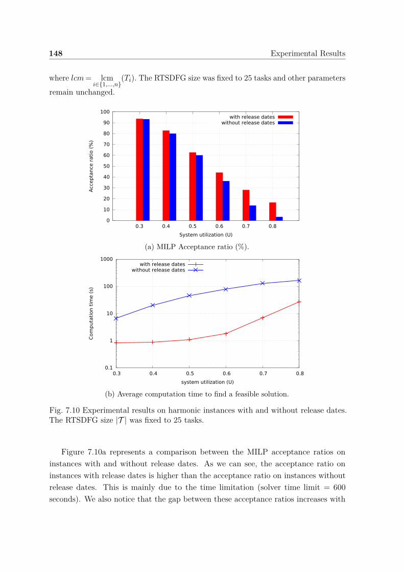
148 Experimental Results
where lcm = lcmi∈1,...,n
(Ti). The RTSDFG size was fixed to 25 tasks and other parametersremain unchanged.
0
10
20
30
40
50
60
70
80
90
100
0.3 0.4 0.5 0.6 0.7 0.8
Acc
ep
tance
rati
o (
%)
System utilization (U)
with release dateswithout release dates
(a) MILP Acceptance ratio (%).
0.1
1
10
100
1000
0.3 0.4 0.5 0.6 0.7 0.8
Com
puta
tion t
ime (
s)
system utilization (U)
with release dateswithout release dates
(b) Average computation time to find a feasible solution.
Fig. 7.10 Experimental results on harmonic instances with and without release dates.The RTSDFG size |T | was fixed to 25 tasks.
Figure 7.10a represents a comparison between the MILP acceptance ratios oninstances with and without release dates. As we can see, the acceptance ratio oninstances with release dates is higher than the acceptance ratio on instances withoutrelease dates. This is mainly due to the time limitation (solver time limit = 600seconds). We also notice that the gap between these acceptance ratios increases with

7.3 Mono-processor scheduling 149
the increase of the system utilization. This is due to the increase of the tasks worstcase execution times.
Figure 7.10b depicts the average computation time to find a feasible schedule forinstances with and without release dates. We notice that the solver requires more timeto find a feasible solution for instances without release dates than instances with releasedates. For example, when the system utilization is fixed to 0.7, the solver requires onaverage 6.9 seconds to find a feasible schedule for instances with release dates while itrequires 130.68 seconds for instances without release dates. This is because the solverrequires more time to allocate the tasks to a restricted space.
7.3.3 Heuristics
In this subsection, we expose the experimental results of our heuristics: LP relaxation,simple and ACAP. Some instances that cannot be solved by one heuristic, can bescheduled by the other heuristics. Consequently, we propose a mega-heuristic “Mega”that combines several heuristics. Given an RTSDFG instance, this mega-heuristicapplies sequentially the simple and ACAP heuristics for the fixed case. In addition,it applies the LP relaxation, simple and ACAP heuristics for the flexible case. Inboth cases, it either returns a feasible solution or a partial solution that contains aset of tasks that can be scheduled on the same processor. In order to evaluate theirperformances compared to the exact methods, heuristics were only tested on feasibleinstances (that admit feasible schedules using the exact methods) and solver failureinstances. Finally, heuristics were applied on all the instances without any exceptionin order to compare their performances for the fixed and flexible cases.
Complexity
In the simple heuristic, the main computation part of the algorithm is composed ofdouble loops. The inner loop iterates on the interval of length (Di−Ci) in order to finda starting date that allows the task to be scheduled on the processor. The outer loopiterates on all the tasks in the system (|T |). Hence, the simple heuristic complexity isO(|T | · lmax) where lmax = max(Di−Ci). However, the ACAP heuristic complexity isO(|T |2 · lmax), since a third loop was added to compute the list of tasks that verify theschedulabily condition with tasks that are already scheduled.

150 Experimental Results
Fixed case
0
10
20
30
40
50
60
70
80
90
100
0.1 0.2 0.3 0.4 0.5 0.6 0.7
Acc
ep
tance
rati
o (
%)
System utilization (U)
MILP
(a) MILP acceptance ratio for the fixed case.
30
40
50
60
70
80
90
100
0.1 0.2 0.3 0.4 0.5 0.6 0.7
Acc
ep
tance
rati
o (
%)
System utilization (U)
MegaACAP
Simple
(b) Heuristics acceptance ratio on feasible instances.
Fig. 7.11 Experimental results on harmonic instances without release dates. TheRTSDFG size |T | was fixed to 30 tasks.
In this experiment, we generated harmonic instances without release dates. The systemutilization was varied between 0.1 and 0.7. The RTSDFG size was fixed to 30 tasks.Using the exact method for the fixed case, instances were sorted into feasible, infeasibleand solver failure. Figure 7.11a presents the MILP acceptance ratio for the fixed case.Figure 7.11b gives the heuristics acceptance ratios on feasible instances. We noticethat the mega-heuristic have a higher acceptance ratio compared to those of the simple

7.3 Mono-processor scheduling 151
and ACAP heuristics. For the three heuristics, we notice that the acceptance ratiosdecrease with the increase of the system utilisation. For example, the Mega acceptanceratio decreases from 99.4% for U = 0.1 to 39.02% for U = 0.7. This is mainly due tothe increase of the tasks worst execution times.
Figure 7.12 depicts the average computation time to find a feasible schedule usingdifferent methods. We notice that our methods have a similar changing tendency, i.e.their average computation times increase with the increase of the system utilization.This is due to the amount of computation that grows with the incrementation ofthe tasks worst execution times. However, our heuristics have computation timesconsiderably lower than the exact method (MILP). For example, when the systemutilization is 0.5, the average computation times of the exact method, Mega, ACAPand simple heuristics are respectively equal to 154.31, 3.02, 15.43 and 2.37 seconds.Therefore, we deduce that the Mega heuristic is 51.09 times faster than the exactmethod (MILP) with an acceptance ratio of 75.25%. On the other hand, we noticethe ACAP heuristic is more time consumption than the simple heuristic. Hence, theexperimental results are compatible with the computational complexity.
0.1
1
10
100
1000
0.1 0.2 0.3 0.4 0.5 0.6 0.7
Com
puta
tion t
ime (
s)
System utilization (U)
MILPMegaACAP
Simple
Fig. 7.12 Average computation time to find a feasible solution. MILP represents ourexact method while Mega, ACAP and simple represent our heuristics.
In the experiment of Figure 7.13b, we apply our heuristics on the solver failureinstances. Figure 7.13a shows the percentage of these instances with respect to thesystem utilization. Similarly to the previous case, the heuristics acceptance ratios
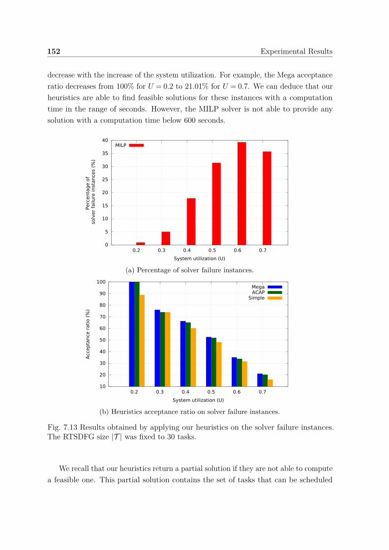
152 Experimental Results
decrease with the increase of the system utilization. For example, the Mega acceptanceratio decreases from 100% for U = 0.2 to 21.01% for U = 0.7. We can deduce that ourheuristics are able to find feasible solutions for these instances with a computationtime in the range of seconds. However, the MILP solver is not able to provide anysolution with a computation time below 600 seconds.
0
5
10
15
20
25
30
35
40
0.2 0.3 0.4 0.5 0.6 0.7
Perc
enta
ge o
f s
olv
er
failu
re inst
ance
s (%
)
System utilization (U)
MILP
(a) Percentage of solver failure instances.
10
20
30
40
50
60
70
80
90
100
0.2 0.3 0.4 0.5 0.6 0.7
Acc
ep
tance
rati
o (
%)
System utilization (U)
MegaACAP
Simple
(b) Heuristics acceptance ratio on solver failure instances.
Fig. 7.13 Results obtained by applying our heuristics on the solver failure instances.The RTSDFG size |T | was fixed to 30 tasks.
We recall that our heuristics return a partial solution if they are not able to computea feasible one. This partial solution contains the set of tasks that can be scheduled
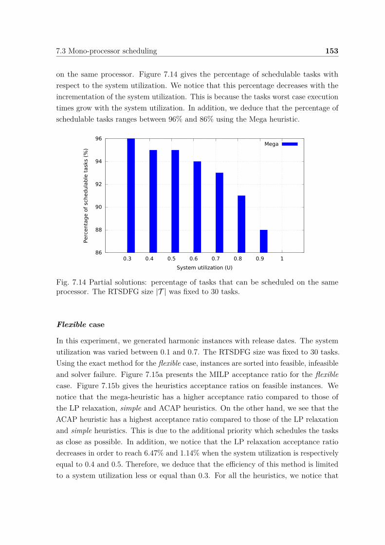
7.3 Mono-processor scheduling 153
on the same processor. Figure 7.14 gives the percentage of schedulable tasks withrespect to the system utilization. We notice that this percentage decreases with theincrementation of the system utilization. This is because the tasks worst case executiontimes grow with the system utilization. In addition, we deduce that the percentage ofschedulable tasks ranges between 96% and 86% using the Mega heuristic.
86
88
90
92
94
96
0.3 0.4 0.5 0.6 0.7 0.8 0.9 1
Perc
enta
ge o
f sc
hedula
ble
task
s (%
)
System utilization (U)
Mega
Fig. 7.14 Partial solutions: percentage of tasks that can be scheduled on the sameprocessor. The RTSDFG size |T | was fixed to 30 tasks.
Flexible case
In this experiment, we generated harmonic instances with release dates. The systemutilization was varied between 0.1 and 0.7. The RTSDFG size was fixed to 30 tasks.Using the exact method for the flexible case, instances are sorted into feasible, infeasibleand solver failure. Figure 7.15a presents the MILP acceptance ratio for the flexiblecase. Figure 7.15b gives the heuristics acceptance ratios on feasible instances. Wenotice that the mega-heuristic has a higher acceptance ratio compared to those ofthe LP relaxation, simple and ACAP heuristics. On the other hand, we see that theACAP heuristic has a highest acceptance ratio compared to those of the LP relaxationand simple heuristics. This is due to the additional priority which schedules the tasksas close as possible. In addition, we notice that the LP relaxation acceptance ratiodecreases in order to reach 6.47% and 1.14% when the system utilization is respectivelyequal to 0.4 and 0.5. Therefore, we deduce that the efficiency of this method is limitedto a system utilization less or equal than 0.3. For all the heuristics, we notice that
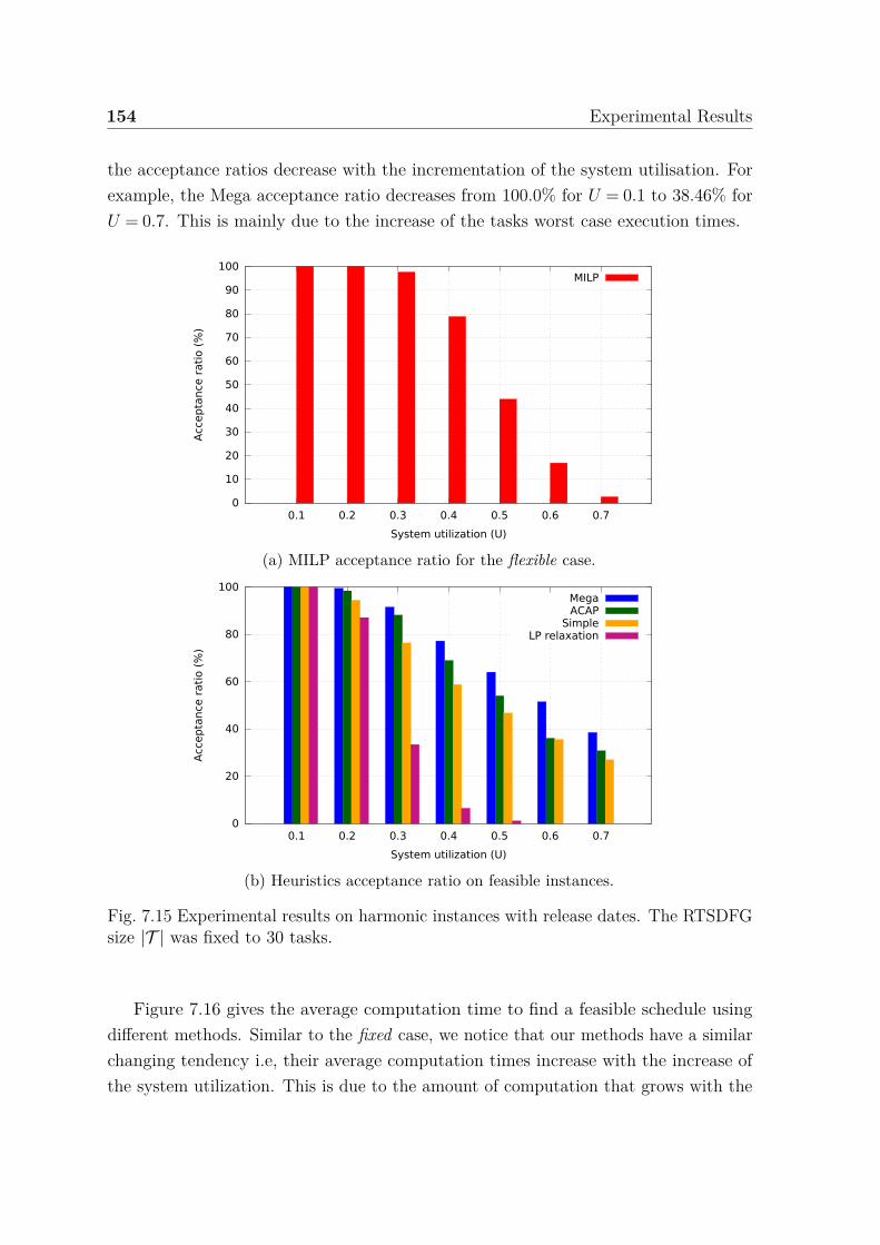
154 Experimental Results
the acceptance ratios decrease with the incrementation of the system utilisation. Forexample, the Mega acceptance ratio decreases from 100.0% for U = 0.1 to 38.46% forU = 0.7. This is mainly due to the increase of the tasks worst case execution times.
0
10
20
30
40
50
60
70
80
90
100
0.1 0.2 0.3 0.4 0.5 0.6 0.7
Acc
ep
tance
rati
o (
%)
System utilization (U)
MILP
(a) MILP acceptance ratio for the flexible case.
0
20
40
60
80
100
0.1 0.2 0.3 0.4 0.5 0.6 0.7
Acc
ep
tance
rati
o (
%)
System utilization (U)
MegaACAP
SimpleLP relaxation
(b) Heuristics acceptance ratio on feasible instances.
Fig. 7.15 Experimental results on harmonic instances with release dates. The RTSDFGsize |T | was fixed to 30 tasks.
Figure 7.16 gives the average computation time to find a feasible schedule usingdifferent methods. Similar to the fixed case, we notice that our methods have a similarchanging tendency i.e, their average computation times increase with the increase ofthe system utilization. This is due to the amount of computation that grows with the
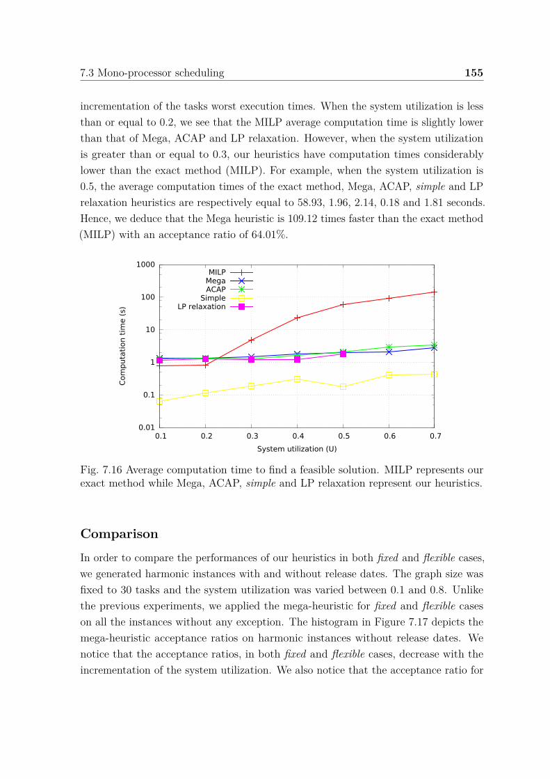
7.3 Mono-processor scheduling 155
incrementation of the tasks worst execution times. When the system utilization is lessthan or equal to 0.2, we see that the MILP average computation time is slightly lowerthan that of Mega, ACAP and LP relaxation. However, when the system utilizationis greater than or equal to 0.3, our heuristics have computation times considerablylower than the exact method (MILP). For example, when the system utilization is0.5, the average computation times of the exact method, Mega, ACAP, simple and LPrelaxation heuristics are respectively equal to 58.93, 1.96, 2.14, 0.18 and 1.81 seconds.Hence, we deduce that the Mega heuristic is 109.12 times faster than the exact method(MILP) with an acceptance ratio of 64.01%.
0.01
0.1
1
10
100
1000
0.1 0.2 0.3 0.4 0.5 0.6 0.7
Com
puta
tion t
ime (
s)
System utilization (U)
MILPMegaACAP
SimpleLP relaxation
Fig. 7.16 Average computation time to find a feasible solution. MILP represents ourexact method while Mega, ACAP, simple and LP relaxation represent our heuristics.
Comparison
In order to compare the performances of our heuristics in both fixed and flexible cases,we generated harmonic instances with and without release dates. The graph size wasfixed to 30 tasks and the system utilization was varied between 0.1 and 0.8. Unlikethe previous experiments, we applied the mega-heuristic for fixed and flexible caseson all the instances without any exception. The histogram in Figure 7.17 depicts themega-heuristic acceptance ratios on harmonic instances without release dates. Wenotice that the acceptance ratios, in both fixed and flexible cases, decrease with theincrementation of the system utilization. We also notice that the acceptance ratio for
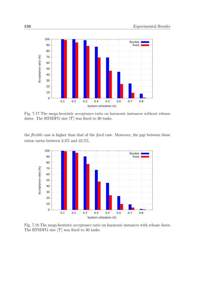
156 Experimental Results
0
10
20
30
40
50
60
70
80
90
100
0.1 0.2 0.3 0.4 0.5 0.6 0.7 0.8
Acc
ep
tance
rati
o (
%)
System utilization (U)
flexiblefixed
Fig. 7.17 The mega-heuristic acceptance ratio on harmonic instances without releasedates. The RTSDFG size |T | was fixed to 30 tasks.
the flexible case is higher than that of the fixed case. Moreover, the gap between theseratios varies between 2.3% and 22.5%.
0
10
20
30
40
50
60
70
80
90
100
0.1 0.2 0.3 0.4 0.5 0.6 0.7 0.8
Acc
epta
nce
rati
o (
%)
System utilization (U)
flexiblefixed
Fig. 7.18 The mega-heuristic acceptance ratio on harmonic instances with release dates.The RTSDFG size |T | was fixed to 30 tasks.
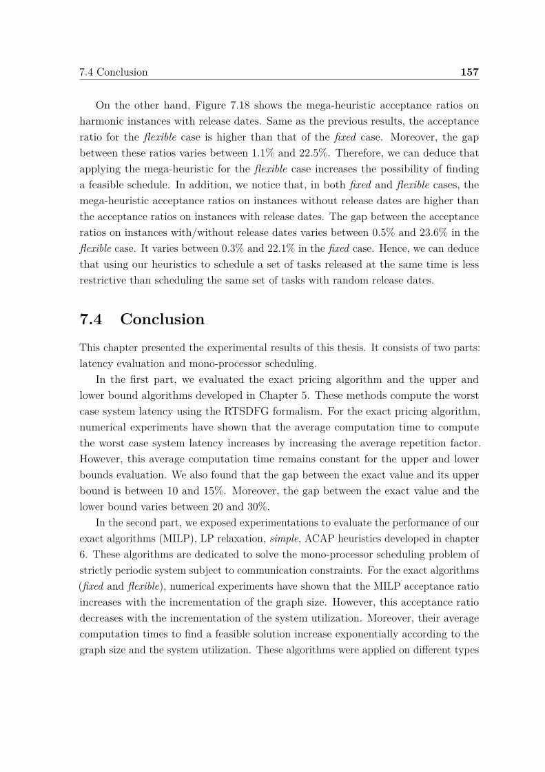
7.4 Conclusion 157
On the other hand, Figure 7.18 shows the mega-heuristic acceptance ratios onharmonic instances with release dates. Same as the previous results, the acceptanceratio for the flexible case is higher than that of the fixed case. Moreover, the gapbetween these ratios varies between 1.1% and 22.5%. Therefore, we can deduce thatapplying the mega-heuristic for the flexible case increases the possibility of findinga feasible schedule. In addition, we notice that, in both fixed and flexible cases, themega-heuristic acceptance ratios on instances without release dates are higher thanthe acceptance ratios on instances with release dates. The gap between the acceptanceratios on instances with/without release dates varies between 0.5% and 23.6% in theflexible case. It varies between 0.3% and 22.1% in the fixed case. Hence, we can deducethat using our heuristics to schedule a set of tasks released at the same time is lessrestrictive than scheduling the same set of tasks with random release dates.
7.4 ConclusionThis chapter presented the experimental results of this thesis. It consists of two parts:latency evaluation and mono-processor scheduling.
In the first part, we evaluated the exact pricing algorithm and the upper andlower bound algorithms developed in Chapter 5. These methods compute the worstcase system latency using the RTSDFG formalism. For the exact pricing algorithm,numerical experiments have shown that the average computation time to computethe worst case system latency increases by increasing the average repetition factor.However, this average computation time remains constant for the upper and lowerbounds evaluation. We also found that the gap between the exact value and its upperbound is between 10 and 15%. Moreover, the gap between the exact value and thelower bound varies between 20 and 30%.
In the second part, we exposed experimentations to evaluate the performance of ourexact algorithms (MILP), LP relaxation, simple, ACAP heuristics developed in chapter6. These algorithms are dedicated to solve the mono-processor scheduling problem ofstrictly periodic system subject to communication constraints. For the exact algorithms(fixed and flexible), numerical experiments have shown that the MILP acceptance ratioincreases with the incrementation of the graph size. However, this acceptance ratiodecreases with the incrementation of the system utilization. Moreover, their averagecomputation times to find a feasible solution increase exponentially according to thegraph size and the system utilization. These algorithms were applied on different types
158 Experimental Results
of instances in order to evaluate the impact of several parameters, such as the periodratio and the graph topology.
On the other hand, we proposed a mega-heuristic that combines several heuristicsfor both fixed and flexible cases. Heuristics were applied on several types of instances.Experimental results showed that the average computation time to find a feasibleschedule using the mega-heuristic is much less compared to the exact method, especiallywhen the system utilization is greater than or equal to 0.5. On the other hand, theseexperiments demonstrate that the mega-heuristic acceptance ratio on solver failureinstances varies between 100% and 21.01% with an average computation time in therange of seconds. In addition, we found that the mega-heuristic is able to allocate onthe same processor 96% to 86% of the tasks when it is not able to provide a feasibleschedule. Finally, we compared the mega-heuristic for both fixed and flexible cases.We found out that the mega-heuristic acceptance ratio for the flexible case is greaterthan the fixed case with a gap which may reach 26.3%.
Chapter 8
Conclusion and Perspectives
ConclusionIn recent decades, electronic embedded systems have revolutionized our societies in dailylives. The increase in the application demands and the fast improvement in platformarchitectures led to more and more complex embedded systems. In order to ensure theoptimal use of resources, several applications from different computing domains aresimultaneously executed on the same platform. Advanced Driver Assistance Systems(ADAS) [117, 66] are typical examples of these applications. Their purpose is to assistdrivers in making safety-related decisions, provide signals in possibly dangerous drivingsituations, and execute counteractive measures. These applications gather best-effortjobs (e.g. image processing for analyzing complex scenes) and critical real-time tasks(e.g. emergency braking). Therefore, this type of applications require a research effortin order to be efficiently modeled and executed. In this thesis, our study was focusedon modeling and scheduling critical real-time systems using data flow formalisms.
In the first part, we defined a general and intuitive communication model withinmulti-periodic systems. We demonstrated that the communications between multi-periodic tasks can be directly expressed as a RTSDFG. This modeling allows precisedefinition of the system latency. Accordingly, we developed an exact evaluation methodto compute the worst case system latency from a given input to a connected outcome.Then, we framed this value using two algorithms that compute its upper and lowerbounds respectively. Finally, our experimental results show that these bounds can becomputed using a polynomial amount of time, while the time required to computethe exact value increases linearly with the average repetition factor. We also foundthat the gap between the exact value and its upper bound varied between 10 and 15%.
160 Conclusion and Perspectives
Moreover, the gap between the exact value and the lower bound varied between 20and 30%.
In the second part, we addressed the mono-processor scheduling problem of non-preemtive strictly periodic systems subject to communication constraints. Based on theRTSDFG model, we proved that scheduling two strictly periodic communicating tasksis equivalent to scheduling two independent tasks. These tasks can only be executedbetween their release dates and their deadlines. Accordingly, we proposed an optimalalgorithm using MILP formulations. Two cases were treated: the fixed and flexibleinterval cases. Since the scheduling problem is know to be NP-complete in the strongsense [79], we proposed three heuristics: linear programming relaxation, simple andACAP heuristics. For the second and the third heuristic if no feasible solution is found,a partial solution is computed. In comparison to the optimal algorithms, heuristics werecharacterized by small average computation times. The heuristics acceptance ratioson feasible instances varied between 100% and 38.46%. Moreover, their acceptanceratios on solver failure instances varied between 100% and 21.01% with an averagecomputation time in the range of seconds. Finally, these heuristics were able to allocateon the same processor 96% to 86% of the tasks when they were not able to provide afeasible schedule.
PerspectivesThis section presents perspectives and potential future work in the continuity of thisthesis.
Multi/Many-processor scheduling
In this thesis, we proposed several heuristics (Mega, ACAP and simple) in order to solvethe mono-processor scheduling problem of non-preemptive strictly periodic systemssubject to communication constraints. These heuristics are much less time-consumingthan the exact methods. In addition, they are able to provide a partial schedule when afeasible schedule is not found. Therefore, one of the perspectives of our work is mappingand scheduling an application modeled by a RTSDFG on a distributed architecturesuch as Kalray-MPPA [3]. This future work can investigate the multi/many-processorscheduling problem while taking into account the inter-processor communications. In

161
fact, our communication model allows us to compute, using a closed formula, the timerequired to transfer data between the tasks’ executions.
Application: WATERS Industrial Challenge
Hamann et al. [57] proposed an automotive embedded application for WATERS Indus-trial Challenge 2017. This application is an engine management system which consistsof several functional components. These latter are tightly related by communicationdependencies and data sharing, while having real-time requirements. This applicationis composed of:
• 1250 runnables which represent pieces of codes that read and write a set of labels.
• 10000 labels that symbolize the communication variables between runnables.Producing (writing) a label is restricted to at most one runnable. However,consuming (reading) a label can be done by several runnables.
• 21 tasks which group several runnables. Periodic tasks gather several runnablesthat have the same period, while sporadic tasks assemble runnables that havethe same minimal and maximal inter arrival times.
Logical Execution Time (LET) has been proposed to ensures temporal determinism bydecoupling computation and communication. In this context, it would be interesting tomodel this application using the RTSDFG formalism, since the communication modelbehind this formalism is similar to the LET concept.
Relax the strict periodicity constraint
In this thesis, we addressed the scheduling problem of non-preemptive strictly periodicsystems subject to communication constraints. The strict periodicity allowed us todefine the resource constraints with a polynomial number of constraints on the startingdates of the tasks’ first executions. Accordingly, we developed an exact method andseveral heuristics that solve the scheduling problem. An interesting perspective isto address the non-preemptive scheduling problem by relaxing the strict periodicityconstraint. This problem can be solved using the list scheduling algorithms [53, 81]. Infact, it would be worth comparing our results, in terms of acceptance ratio and averagecomputation time, to the results obtained by relaxing the strict periodicity constraint.

References
[1] Al Sheikh, A., Brun, O., Hladik, P.-E., and Prabhu, B. J. (2011). A best-responsealgorithm for multiprocessor periodic scheduling. In Real-Time Systems (ECRTS),2011 23rd Euromicro Conference on, pages 228–237. IEEE.
[2] Ali, H. I., Akesson, B., and Pinho, L. M. (2015). Generalized extraction of real-timeparameters for homogeneous synchronous dataflow graphs. In Parallel, Distributedand Network-Based Processing (PDP), 2015 23rd Euromicro International Conferenceon, pages 701–710. IEEE.
[3] Aubry, P., Beaucamps, P.-E., Blanc, F., Bodin, B., Carpov, S., Cudennec, L., David,V., Doré, P., Dubrulle, P., De Dinechin, B. D., et al. (2013). Extended cyclostaticdataflow program compilation and execution for an integrated manycore processor.Procedia Computer Science, 18:1624–1633.
[4] Baccelli, F., Cohen, G., Olsder, G. J., and Quadrat, J.-P. (1992). Synchronizationand linearity: an algebra for discrete event systems.
[5] Bamakhrama, M. and Stefanov, T. (2011). Hard-real-time scheduling of data-dependent tasks in embedded streaming applications. In Proceedings of the ninthACM international conference on Embedded software, pages 195–204. ACM.
[6] Bamakhrama, M. A. and Stefanov, T. (2012). Managing latency in embeddedstreaming applications under hard-real-time scheduling. In Proceedings of the eighthIEEE/ACM/IFIP international conference on Hardware/software codesign and sys-tem synthesis, pages 83–92. ACM.
[7] Bamakhrama, M. A., Zhai, J. T., Nikolov, H., and Stefanov, T. (2012). A method-ology for automated design of hard-real-time embedded streaming systems. InProceedings of the Conference on Design, Automation and Test in Europe, pages941–946. EDA Consortium.
[8] Baruah, S. (2007). Techniques for multiprocessor global schedulability analysis. InReal-Time Systems Symposium, 2007. RTSS 2007. 28th IEEE International, pages119–128. IEEE.
[9] Baruah, S. K. (2006). The non-preemptive scheduling of periodic tasks uponmultiprocessors. Real-Time Systems, 32(1):9–20.
[10] Baruah, S. K., Mok, A. K., and Rosier, L. E. (1990a). Preemptively schedulinghard-real-time sporadic tasks on one processor. In Real-Time Systems Symposium,1990. Proceedings., 11th, pages 182–190. IEEE.
164 References
[11] Baruah, S. K., Rosier, L. E., and Howell, R. R. (1990b). Algorithms and complexityconcerning the preemptive scheduling of periodic, real-time tasks on one processor.Real-time systems, 2(4):301–324.
[12] Benabid-Najjar, A., Hanen, C., Marchetti, O., and Munier-Kordon, A. (2012).Periodic schedules for bounded timed weighted event graphs. IEEE Transactions onAutomatic Control, 57(5):1222–1232.
[13] Benveniste, A., Le Guernic, P., and Jacquemot, C. (1991). Synchronous program-ming with events and relations: the signal language and its semantics. Science ofcomputer programming, 16(2):103–149.
[14] Bernat, G., Burns, A., and Liamosi, A. (2001). Weakly hard real-time systems.IEEE Transactions on Computers, 50(4):308–321.
[15] Berry, G. (1989). Real time programming: Special purpose or general purposelanguages. PhD thesis, INRIA.
[16] Berry, G. and Gonthier, G. (1992). The esterel synchronous programming language:Design, semantics, implementation. Science of computer programming, 19(2):87–152.
[17] Bilsen, G., Engels, M., Lauwereins, R., and Peperstraete, J. (1996). Cycle-staticdataflow. IEEE Transactions on signal processing, 44(2):397–408.
[18] Bini, E. and Buttazzo, G. C. (2005). Measuring the performance of schedulabilitytests. Real-Time Systems, 30(1-2):129–154.
[19] Bodin, B., Lesparre, Y., Delosme, J.-M., and Munier-Kordon, A. (2014). Fastand efficient dataflow graph generation. In Proceedings of the 17th InternationalWorkshop on Software and Compilers for Embedded Systems, pages 40–49. ACM.
[20] Bouakaz, A., Talpin, J.-P., and Vitek, J. (2012). Affine data-flow graphs for thesynthesis of hard real-time applications. In Application of Concurrency to SystemDesign (ACSD), 2012 12th International Conference on, pages 183–192. IEEE.
[21] Brandes, U. (2001). A faster algorithm for betweenness centrality. Journal ofmathematical sociology, 25(2):163–177.
[22] Burns, A. and Wellings, A. J. (2001). Real-time systems and programming lan-guages: Ada 95, real-time Java, and real-time POSIX. Pearson Education.
[23] Caspi, P., Mazuet, C., and Paligot, N. (2001). About the design of distributedcontrol systems: The quasi-synchronous approach. Computer Safety, Reliability andSecurity, pages 215–226.
[24] Chabrol, D., David, V., Aussagues, C., Louise, S., and Daumas, F. (2005). Deter-ministic distributed safety-critical real-time systems within the oasis approach. InIASTED PDCS, pages 260–268.
[25] Chen, J., Du, C., Xie, F., and Lin, B. (2016a). Allocation and scheduling ofstrictly periodic tasks in multi-core real-time systems. In Embedded and Real-TimeComputing Systems and Applications (RTCSA), 2016 IEEE 22nd InternationalConference on, pages 130–138. IEEE.

References 165
[26] Chen, J., Du, C., Xie, F., and Yang, Z. (2016b). Schedulability analysis ofnon-preemptive strictly periodic tasks in multi-core real-time systems. Real-TimeSystems, 52(3):239–271.
[27] Cohen, A., Duranton, M., Eisenbeis, C., Pagetti, C., Plateau, F., and Pouzet, M.(2006). N-synchronous kahn networks: a relaxed model of synchrony for real-timesystems. ACM SIGPLAN Notices, 41(1):180–193.
[28] Cohen, G., Dubois, D., Quadrat, J., and Viot, M. (1985). A linear-system-theoretic view of discrete-event processes and its use for performance evaluation inmanufacturing. IEEE transactions on Automatic Control, 30(3):210–220.
[29] Cucu, L. and Sorel, Y. (2003). Schedulability condition for systems with precedenceand periodicity constraints without preemption. In Proceedings of 11th Real-TimeSystems Conference, RTS’03.
[30] Cucu, L. and Sorel, Y. (2004). Non-preemptive multiprocessor scheduling forstrict periodic systems with precedence constraints.
[31] Dantzig, G. B. and Wolfe, P. (1960). Decomposition principle for linear programs.Operations research, 8(1):101–111.
[32] Davis, A. L. and Keller, R. M. (1982). Data flow program graphs.
[33] Davis, R. I. and Burns, A. (2011). A survey of hard real-time scheduling formultiprocessor systems. ACM computing surveys (CSUR), 43(4):35.
[34] Dennis, J. B. (1974). First version of a data flow procedure language. In Program-ming Symposium, pages 362–376. Springer.
[35] Do, X. K. (2016). Modèle de calcul et d’exécution pour des applications flots dedonnées dynamiques avec contraintes temps réel. PhD thesis, Paris 6.
[36] Do, X. K., Louise, S., and Cohen, A. (2015). Managing the latency of data-dependent tasks in embedded streaming applications. In Embedded Multicore/Many-core Systems-on-Chip (MCSoC), 2015 IEEE 9th International Symposium on, pages9–16. IEEE.
[37] Eisenbrand, F., Hähnle, N., Niemeier, M., Skutella, M., Verschae, J., and Wiese,A. (2010a). Scheduling periodic tasks in a hard real-time environment. Automata,languages and programming, pages 299–311.
[38] Eisenbrand, F., Kesavan, K., Mattikalli, R. S., Niemeier, M., Nordsieck, A. W.,Skutella, M., Verschae, J., and Wiese, A. (2010b). Solving an avionics real-timescheduling problem by advanced ip-methods. In European Symposium on Algorithms,pages 11–22. Springer.
[39] Elloy, J.-P. (1991). Les contraintes du temps réel dans les systèmes industrielsrépartis. Revue générale de l’électricité, (2):26–30.
[40] Feiler, P. H., Gluch, D. P., and Hudak, J. J. (2006). The architecture analysis &design language (aadl): An introduction. Technical report, Carnegie-Mellon UnivPittsburgh PA Software Engineering Inst.

166 References
[41] Forget, J. (2009). A synchronous language for critical embedded systems withmultiple real-time constraints. Ph. D. dissertation.
[42] Forget, J., Boniol, F., Lesens, D., and Pagetti, C. (2008). A multi-periodicsynchronous data-flow language. In High Assurance Systems Engineering Symposium,2008. HASE 2008. 11th IEEE, pages 251–260. IEEE.
[43] Forget, J., Boniol, F., Lesens, D., and Pagetti, C. (2010). A real-time architecturedesign language for multi-rate embedded control systems. In Proceedings of the 2010ACM Symposium on Applied Computing, pages 527–534. ACM.
[44] Fudenberg, D. and Tirole, J. (1991). Game theory. Technical report, The MITpress.
[45] George, L., Rivierre, N., and Spuri, M. (1996). Preemptive and non-preemptivereal-time uniprocessor scheduling. PhD thesis, Inria.
[46] Gilles, K. (1974). The semantics of a simple language for parallel programming.Information processing, 74:471–475.
[47] Girault, A., Kalla, H., and Sorel, Y. (2003). Une heuristique d’ordonnancement etde distribution tolérante aux pannes pour systemes temps-réel embarqués. Modélisa-tion des Systemes Réactifs, MSR’03, pages 145–160.
[48] Goddard, S. (1997). Analyzing the real-time properties of a dataflow executionparadigm using a synthetic aperture radar application. In Real-Time Technologyand Applications Symposium, 1997. Proceedings., Third IEEE, pages 60–71. IEEE.
[49] Goossens, J. (2003). Scheduling of offset free systems. Real-Time Systems,24(2):239–258.
[50] Goossens, J. and Macq, C. (2001). Limitation of the hyper-period in real-timeperiodic task set generation. In In Proceedings of the RTS Embedded System (RTS’01.Citeseer.
[51] Goossens, K., Azevedo, A., Chandrasekar, K., Gomony, M. D., Goossens, S.,Koedam, M., Li, Y., Mirzoyan, D., Molnos, A., Nejad, A. B., et al. (2013). Virtualexecution platforms for mixed-time-criticality systems: the compsoc architectureand design flow. ACM SIGBED Review, 10(3):23–34.
[52] Goubier, T., Sirdey, R., Louise, S., and David, V. (2011). σc: A programmingmodel and language for embedded manycores. In International Conference onAlgorithms and Architectures for Parallel Processing, pages 385–394. Springer.
[53] Graham, R. L. (1966). Bounds for certain multiprocessing anomalies. Bell LabsTechnical Journal, 45(9):1563–1581.
[54] Grandpierre, T., Lavarenne, C., and Sorel, Y. (1999). Optimized rapid prototypingfor real-time embedded heterogeneous multiprocessors. In Proceedings of the seventhinternational workshop on Hardware/software codesign, pages 74–78. ACM.

References 167
[55] Guan, N., Yi, W., Deng, Q., Gu, Z., and Yu, G. (2011). Schedulability analysisfor non-preemptive fixed-priority multiprocessor scheduling. Journal of SystemsArchitecture, 57(5):536–546.
[56] Halbwachs, N., Caspi, P., Raymond, P., and Pilaud, D. (1991). The synchronousdata flow programming language lustre. Proceedings of the IEEE, 79(9):1305–1320.
[57] Hamann, A., Dasari, D., Kramer, S., Pressler, M., Wurst, F., and Ziegenbein, D.(2017). Waters industrial challenge 2017.
[58] Harel, D. and Pnueli, A. (1985). On the development of reactive systems. WeizmannInstitute of Science. Department of Applied Mathematics.
[59] Hausmans, J. P., Geuns, S. J., Wiggers, M. H., and Bekooij, M. J. (2014). Temporalanalysis flow based on an enabling rate characterization for multi-rate applicationsexecuted on mpsocs with non-starvation-free schedulers. In Proceedings of the 17thInternational Workshop on Software and Compilers for Embedded Systems, pages108–117. ACM.
[60] Hausmans, J. P., Wiggers, M. H., Geuns, S. J., and Bekooij, M. J. (2013).Dataflow analysis for multiprocessor systems with non-starvation-free schedulers.In Proceedings of the 16th International Workshop on Software and Compilers forEmbedded Systems, pages 13–22. ACM.
[61] Henzinger, T. A., Horowitz, B., and Kirsch, C. M. (2003a). Giotto: a time-triggeredlanguage for embedded programming. Proceedings of the IEEE, 91(1):84–99.
[62] Henzinger, T. A., Horowitz, B., and Kirsch, C. M. (2003b). Giotto: A time-triggered language for embedded programming. Proceedings of the IEEE, 91(1):84–99.
[63] Hoffman, K. and Padberg, M. (1985). Lp-based combinatorial problem solving.In Computational Mathematical Programming, pages 55–123. Springer.
[64] Hyman, J. M., Lazar, A. A., and Pacifici, G. (1991). Real-time scheduling withquality of service constraints. IEEE Journal on Selected Areas in Communications,9(7):1052–1063.
[65] Jeffay, K., Stanat, D. F., and Martel, C. U. (1991). On non-preemptive schedulingof period and sporadic tasks. In Real-Time Systems Symposium, 1991. Proceedings.,Twelfth, pages 129–139. IEEE.
[66] Jones, W. D. (2002). Building safer cars. IEEE Spectrum, 39(1):82–85.
[67] Jonkman, J. M. and Buhl Jr, M. L. (2005). Fast user’s guide-updated august 2005.Technical report, National Renewable Energy Laboratory (NREL), Golden, CO.
[68] Kantorovich, L. V. (1960). Mathematical methods of organizing and planningproduction. Management Science, 6(4):366–422.
[69] Karp, R. M. and Miller, R. E. (1966). Properties of a model for parallel computa-tions: Determinacy, termination, queueing. SIAM Journal on Applied Mathematics,14(6):1390–1411.
168 References
[70] Kermia, O., Cucu, L., and Sorel, Y. (2006). Non-preemptive multiprocessorstatic scheduling for systems with precedence and strict periodicity constraints.In Proceedings of the 10th International Workshop On Project Management andScheduling, PMS’06.
[71] Kermia, O. and Sorel, Y. (2007). A rapid heuristic for scheduling non-preemptivedependent periodic tasks onto multiprocessor. In Proceedings of ISCA 20th interna-tional conference on Parallel and Distributed Computing Systems, PDCS’07.
[72] Kermia, O. and Sorel, Y. (2008). Schedulability analysis for non-preemptive tasksunder strict periodicity constraints. In Embedded and Real-Time Computing Systemsand Applications, 2008. RTCSA’08. 14th IEEE International Conference on, pages25–32. IEEE.
[73] Khatib, J., Munier-Kordon, A., Klikpo, E. C., and Trabelsi-Colibet, K. (2016).Computing latency of a real-time system modeled by synchronous dataflow graph.In Proceedings of the 24th International Conference on Real-Time Networks andSystems, pages 87–96. ACM.
[74] Kirsch, C. M. (2002). Principles of real-time programming. In EMSOFT, volume 2,pages 61–75. Springer.
[75] Kirsch, C. M., Sanvido, M. A., Henzinger, T. A., and Pree, W. (2002). A giotto-based helicopter control system. In International Workshop on Embedded Software,pages 46–60. Springer.
[76] Klikpo, E. C., Khatib, J., and Munier-Kordon, A. (2016). Modeling multi-periodicsimulink systems by synchronous dataflow graphs. In Real-Time and EmbeddedTechnology and Applications Symposium (RTAS), 2016 IEEE, pages 1–10. IEEE.
[77] Kopetz, H. (2002). Time-triggered real-time computing. IFAC Proceedings Volumes,35(1):59–70.
[78] Kopetz, H. (2011). Real-time systems: design principles for distributed embeddedapplications. Springer Science & Business Media.
[79] Korst, J., Aarts, E., and Lenstra, J. K. (1996). Scheduling periodic tasks. IN-FORMS journal on Computing, 8(4):428–435.
[80] Korst, J., Aarts, E., Lenstra, J. K., and Wessels, J. (1991). Periodic multiprocessorscheduling. In PARLE’91 Parallel Architectures and Languages Europe, pages166–178. Springer.
[81] Kwok, Y.-K. and Ahmad, I. (1999). Benchmarking and comparison of thetask graph scheduling algorithms. Journal of Parallel and Distributed Comput-ing, 59(3):381–422.
[82] Land, A. H. and Doig, A. G. (2010). An automatic method for solving discreteprogramming problems. 50 Years of Integer Programming 1958-2008, pages 105–132.
[83] Lee, E. and Messerschmitt, D. (1987a). Synchronous data flow. Proceedings of theIEEE, 75(9):1235–1245.

References 169
[84] Lee, E. A. and Messerschmitt, D. G. (1987b). Static scheduling of synchronousdata flow programs for digital signal processing. IEEE Transactions on computers,100(1):24–35.
[85] Liu, C. L. and Layland, J. W. (1973). Scheduling algorithms for multiprogrammingin a hard-real-time environment. Journal of the ACM (JACM), 20(1):46–61.
[86] Liu, D., Spasic, J., Zhai, J. T., Stefanov, T., and Chen, G. (2014). Resourceoptimization for csdf-modeled streaming applications with latency constraints. InDesign, Automation and Test in Europe Conference and Exhibition (DATE), 2014,pages 1–6. IEEE.
[87] Louise, S., David, V., Delcoigne, J., and Aussagues, C. (2002). Oasis project:deterministic real-time for safety critical embedded systems. In Proceedings of the10th workshop on ACM SIGOPS European workshop, pages 223–226. ACM.
[88] Magnanti, T. L. and Vachani, R. (1990). A strong cutting plane algorithm forproduction scheduling with changeover costs. Operations Research, 38(3):456–473.
[89] Mandel, L., Plateau, F., and Pouzet, M. (2010). Lucy-n: a n-synchronous extensionof lustre. In MPC, volume 6120, pages 288–309. Springer.
[90] Marchetti, O. and Kordon, A. M. (2009). Cyclic scheduling for the synthesis ofembedded systems. Introduction to scheduling, pages 135–164.
[91] Marchetti, O. and Munier-Kordon, A. (2009). A sufficient condition for the livenessof weighted event graphs. European Journal of Operational Research, 197(2):532–540.
[92] Marouf, M. and Sorel, Y. (2010). Schedulability conditions for non-preemptive hardreal-time tasks with strict period. In 18th International Conference on Real-Timeand Network Systems RTNS’10.
[93] Marouf, M. and Sorel, Y. (2011). Scheduling non-preemptive hard real-time taskswith strict periods. In Emerging Technologies & Factory Automation (ETFA), 2011IEEE 16th Conference on, pages 1–8. IEEE.
[94] Mok, A. K.-L. (1983). Fundamental design problems of distributed systems for thehard-real-time environment. PhD thesis, Massachusetts Institute of Technology.
[95] Moreira, O. M. and Bekooij, M. J. (2007). Self-timed scheduling analysisfor real-time applications. EURASIP Journal on Advances in Signal Processing,2007(1):083710.
[96] Munier, A. (1993). Optimal asymptotic behavior of a generalized timed eventgraph: application to an assembly system. APII, 27:487–487.
[97] Nasri, M., Baruah, S., Fohler, G., and Kargahi, M. (2014). On the optimality ofrm and edf for non-preemptive real-time harmonic tasks. In Proceedings of the 22ndInternational Conference on Real-Time Networks and Systems, page 331. ACM.
[98] Nasri, M. and Kargahi, M. (2014). Precautious-rm: a predictable non-preemptivescheduling algorithm for harmonic tasks. Real-Time Systems, 50(4):548–584.

170 References
[99] Park, C. and Shaw, A. C. (1990). Experiments with a program timing tool basedon source-level timing schema. In Real-Time Systems Symposium, 1990. Proceedings.,11th, pages 72–81. IEEE.
[100] Park, M. (2007). Non-preemptive fixed priority scheduling of hard real-timeperiodic tasks. Computational Science–ICCS 2007, pages 881–888.
[101] Piaggio, M., Sgorbissa, A., and Zaccaria, R. (2000). Pre-emptive versus non-pre-emptive real time scheduling in intelligent mobile robotics. Journal of Experimental& Theoretical Artificial Intelligence, 12(2):235–245.
[102] Pira, C. and Artigues, C. (2013). Propagation mechanism for a non-preemptivestrictly periodic scheduling problem.
[103] Pouzet, M. (2006). Lucid synchrone, version 3. Tutorial and reference manual.Université Paris-Sud, LRI.
[104] Puschner, P. and Koza, C. (1989). Calculating the maximum execution time ofreal-time programs. Real-time systems, 1(2):159–176.
[105] Savelsbergh, M. (1997). A branch-and-price algorithm for the generalized assign-ment problem. Operations research, 45(6):831–841.
[106] Shaw, A. C. (1989). Reasoning about time in higher-level language software.IEEE Transactions on Software Engineering, 15(7):875–889.
[107] Sifakis, J., Tripakis, S., and Yovine, S. (2003). Building models of real-timesystems from application software. Proceedings of the IEEE, 91(1):100–111.
[108] Sih, G. C. and Lee, E. A. (1990). Scheduling to account for interprocessorcommunication within interconnection-constrained processor networks. In ICPP (1),pages 9–16.
[109] Singh, A., Ekberg, P., and Baruah, S. (2017). Applying real-time schedulingtheory to the synchronous data flow model of computation. In LIPIcs-Leibniz Inter-national Proceedings in Informatics, volume 76. Schloss Dagstuhl-Leibniz-Zentrumfuer Informatik.
[110] Sprunt, B., Sha, L., and Lehoczky, J. (1989). Aperiodic task scheduling forhard-real-time systems. Real-Time Systems, 1(1):27–60.
[111] Stankovic, J. A. (1988). Misconceptions about real-time computing: a seriousproblem for next-generation systems. Computer, 21(10):10–19.
[112] Stuijk, S., Geilen, M., and Basten, T. (2006). Exploring trade-offs in bufferrequirements and throughput constraints for synchronous dataflow graphs. In DesignAutomation Conference, 2006 43rd ACM/IEEE, pages 899–904. IEEE.
[113] Tabuada, P. (2007). Event-triggered real-time scheduling of stabilizing controltasks. IEEE Transactions on Automatic Control, 52(9):1680–1685.

References 171
[114] Tendulkar, P., Poplavko, P., and Maler, O. (2014). Strictly periodic scheduling ofacyclic synchronous dataflow graphs using smt solvers. Technical report, Technicalreport TR-2014-5. Verimag research report.
[115] Thies, W., Karczmarek, M., and Amarasinghe, S. (2002a). Streamit: A languagefor streaming applications. In Compiler Construction, pages 49–84. Springer.
[116] Thies, W., Lin, J., and Amarasinghe, S. (2002b). Phased computation graphs inthe polyhedral model.
[117] Vlacic, L., Parent, M., and Harashima, F. (2001). Intelligent vehicle technologies.Butterworth-Heinemann.
[118] Wirth, N. (1977). Toward a discipline of real-time programming. Communicationsof the ACM, 20(8):577–583.