Clemson UniversityTigerPrints

All Theses Theses

5-2016

Modeling and Parameter Estimation of EscherichiaColi BioprocessAjay PadmakumarClemson University, ajaypadmakumar@gmail.com

Follow this and additional works at: https://tigerprints.clemson.edu/all_theses

This Thesis is brought to you for free and open access by the Theses at TigerPrints. It has been accepted for inclusion in All Theses by an authorizedadministrator of TigerPrints. For more information, please contact kokeefe@clemson.edu.

Recommended CitationPadmakumar, Ajay, "Modeling and Parameter Estimation of Escherichia Coli Bioprocess" (2016). All Theses. 2448.https://tigerprints.clemson.edu/all_theses/2448

Abstract

Most biopharmaceuticals today are focused on the production of one of three

major cell types: the bacterium Escherichia coli, yeasts (Saccharomyces cerevisiae,

Pichia pastoris) and mammalian cells (Chinese Hamster Ovary cells). Growth opti-

mization is a major focus as this dictates the pace of advancements in drug manu-

facturing. The process involved in producing these cells itself is very complex and

modeling a system to accurately capture these characteristics can be difficult. The

overall process is expensive to run and repeated testing of various control algorithms

to optimize growth can prove to be very time consuming as well. In order to develop

control strategies and improve the yield of protein, it is beneficial to model a system

that captures the responses of the bioprocess. The model can be coupled with different

controllers to test the yield output and determine the most effective control strategies

without incurring additional costs or time delays. Model parameters are determined

by the process of numerical minimization, making use of experimentally obtained

data to ensure accurate simulation system behavior. Additionally, a separate system

can be developed to switch between the simulation platform and the actual process,

with the same control strategy being implemented to compare against results of the

simulation and the actual process. This allows for further adjustments to be made

to more effectively model the bioprocess. This thesis describes the implementation of

the Xu model, found in literature as the simulation counterpart to an experimental

ii

hardware setup. A hardware-in-the-loop simulation is developed with the ability to

accurately model system parameters against experimentally obtained results in order

to carry out control strategy testing on the simulation side before switching to the

experimental hardware side. Accurate parameter estimation is achieved by fitting

simulation results to experimentally logged data to ensure the simulation replicates

the behavior of the physical system, and is subsequently verified against non-training

data.

iii

Acknowledgments

I would like to sincerely thank my advisor Dr. Richard Groff for his guidance

and feedback. I also thank Dr. Timothy Burg and Dr. Sarah Harcum for their

advice and assistance. I would also like to add a special thanks to Dr. Rod Harrell.

In addition, I would also like to express my gratitude to the other members of this

project, Matthew Pepper and Li Wang for their invaluable support. Finally, I want

thank Harshawardhan Karve for his insight and help.

v

Table of Contents

Title Page . . . . . . . . . . . . . . . . . . . . . . . . . . . . . . . . . . . i

Abstract . . . . . . . . . . . . . . . . . . . . . . . . . . . . . . . . . . . . ii

Dedication . . . . . . . . . . . . . . . . . . . . . . . . . . . . . . . . . . . iv

Acknowledgments . . . . . . . . . . . . . . . . . . . . . . . . . . . . . . . v

List of Tables . . . . . . . . . . . . . . . . . . . . . . . . . . . . . . . . . viii

List of Figures . . . . . . . . . . . . . . . . . . . . . . . . . . . . . . . . . ix

1 Introduction . . . . . . . . . . . . . . . . . . . . . . . . . . . . . . . . 11.1 Background and Motivation . . . . . . . . . . . . . . . . . . . . . . . 11.2 Problem Statement . . . . . . . . . . . . . . . . . . . . . . . . . . . . 21.3 Literature Review . . . . . . . . . . . . . . . . . . . . . . . . . . . . . 21.4 Outline . . . . . . . . . . . . . . . . . . . . . . . . . . . . . . . . . . . 3

2 Design and Methods . . . . . . . . . . . . . . . . . . . . . . . . . . . 52.1 Bioreactor Model . . . . . . . . . . . . . . . . . . . . . . . . . . . . . 5

3 Setup . . . . . . . . . . . . . . . . . . . . . . . . . . . . . . . . . . . . 153.1 Bioreactor Setup . . . . . . . . . . . . . . . . . . . . . . . . . . . . . 153.2 Simulation Model . . . . . . . . . . . . . . . . . . . . . . . . . . . . . 203.3 Configuring Simulation Models . . . . . . . . . . . . . . . . . . . . . 25

4 Experimental Procedure . . . . . . . . . . . . . . . . . . . . . . . . . 28

5 Experimental Results . . . . . . . . . . . . . . . . . . . . . . . . . . . 335.1 Numerical Minimization . . . . . . . . . . . . . . . . . . . . . . . . . 335.2 Fitting Limitations . . . . . . . . . . . . . . . . . . . . . . . . . . . . 405.3 Result Analysis . . . . . . . . . . . . . . . . . . . . . . . . . . . . . . 41

6 Conclusion and Future Work . . . . . . . . . . . . . . . . . . . . . . 46

vi

Appendices . . . . . . . . . . . . . . . . . . . . . . . . . . . . . . . . . . . 49A FermSim Model . . . . . . . . . . . . . . . . . . . . . . . . . . . . . . 50B Experiment Details . . . . . . . . . . . . . . . . . . . . . . . . . . . . 54

Bibliography . . . . . . . . . . . . . . . . . . . . . . . . . . . . . . . . . . 56

vii

List of Tables

2.1 Xu model variables. . . . . . . . . . . . . . . . . . . . . . . . . . . . . 14

3.1 List of sensors and communication protocols used. . . . . . . . . . . . 20

5.1 Estimation parameter description. . . . . . . . . . . . . . . . . . . . . 345.2 Growth block parameter numerical minimization best fit values. . . . 405.3 Error comparison for Fitted vs Xu parameters for the verification ex-

periment. . . . . . . . . . . . . . . . . . . . . . . . . . . . . . . . . . 415.4 Objective function weights for each term. . . . . . . . . . . . . . . . . 44

1 List of sensors and communication protocols used. . . . . . . . . . . . 532 List of all online and offline variables recorded in database. Experiment

number is denoted by i. . . . . . . . . . . . . . . . . . . . . . . . . . 55

viii

List of Figures

2.1 Representation of glucose and oxygen uptake during Oxidative-Overflow,Oxidative-Metabolite Consumption and Oxidative phases of E. colimetabolism. . . . . . . . . . . . . . . . . . . . . . . . . . . . . . . . . 8

2.2 Representation of glucose metabolism during aerobic overflow in E. coli . 112.3 Representation of acetate metabolism during aerobic overflow in E. coli . 12

3.1 Block diagram of overall setup with added sensors. . . . . . . . . . . 163.2 Block properties of the OPC read block from the OPC toolbox in

Matlab/Simulink. . . . . . . . . . . . . . . . . . . . . . . . . . . . . . 183.3 Block properties of the OPC write block from the OPC toolbox in

Matlab/Simulink. . . . . . . . . . . . . . . . . . . . . . . . . . . . . . 193.4 User Interface developed along with FermCtrl for easy read/write ac-

cess of the OPC server variables. . . . . . . . . . . . . . . . . . . . . 263.5 Representation of the Simulink model FermSim along with the input

and output variables. . . . . . . . . . . . . . . . . . . . . . . . . . . . 27

4.1 Experimental setup of the bioreactor and related sensors. 1: Glucosebalance; 2: Glucose bottle; 3: Bioreactor vessel; 4: DO probe; 5: Stirmotor; 6: pH probe; 7: Base balance; 8: Base bottle; 9: Mass flowcontroller; 10: DCU pumps (top to bottom - acid, glucose, antifoam,base); 11: Bluesens off-gas sensor; 12: DCU; 13: xPC target. [3] . . . 29

4.2 A plot of DO (percent), Stir speed (rpm), pH, Temperature (degree C)and Mass flow (L/min) versus Time(h). . . . . . . . . . . . . . . . . . 31

4.3 A plot of O2 (percent), Glucose balance reading (g), Base balance read-ing (g), Acetate concentration offline measurement (g/L) and Glucoseconcentration offline measurement (g/L) versus Time (h). . . . . . . . 32

5.1 Training experiment 1 plots for A, S, X and OUR using fitted param-eters. . . . . . . . . . . . . . . . . . . . . . . . . . . . . . . . . . . . . 37

5.2 Training experiment 2 plots for A, S, X and OUR using fitted param-eters. . . . . . . . . . . . . . . . . . . . . . . . . . . . . . . . . . . . . 38

5.3 Training experiment 3 plots for A, S, X and OUR using fitted param-eters. . . . . . . . . . . . . . . . . . . . . . . . . . . . . . . . . . . . . 39

5.4 Verification experiment plots for A, S, X and OUR using fitted pa-rameters. . . . . . . . . . . . . . . . . . . . . . . . . . . . . . . . . . . 42

ix

5.5 Verification experiment plots for A, S, X and OUR using Xu parameters. 43

1 Simulink model FermSim with input and output variables. . . . . . . 502 FermSim with an example control model. . . . . . . . . . . . . . . . . 513 The S sub-module block. . . . . . . . . . . . . . . . . . . . . . . . . . 52

x

Chapter 1

Introduction

1.1 Background and Motivation

The primary aim of E. coli fermentation processes is to maximize biomass

yield, with the assumption that more biomass equals more product [1]. Many factors

can affect the growth rate of E. coli , including temperature, pH, oxygen uptake rate

(OUR), acetate levels and substrate feed rates. Testing control strategies to deter-

mine maximum yield profiles can be time consuming and costly. Simulated models

offer a means to test such strategies without investing large amounts of time and

capital. Modeling and parameter estimation of the E. coli metabolic process is very

beneficial for implementing and testing control strategies aimed at achieving growth

optimization. Developing a complete simulation model that mimics the real-world

responses of the system, will significantly decrease time and cost involved in conven-

tional testing. Developing this model to run in parallel to the experimental hardware

setup and switching between the hardware and simulation allows easy comparison of

performances as well as improved system dynamics characterization.

1

1.2 Problem Statement

Modeling and parameter estimation of the E. coli metabolic process is very

beneficial for implementing and testing control strategies aimed at achieving growth

optimization. A complete simulation model that mimics the real-world responses of

the system, will significantly decrease time and cost involved in conventional testing,

but can be difficult to implement as there are a lot of factors that need to be included

for the system response to resemble the actual culture response including sensor

measurement delays, strain on culture due to inhibitory elements and measurement

noise. This thesis describes the implementation of the Xu model [2] along with OUR

estimation [3] to model E. coli dynamics. Additionally, estimation of metabolic

parameters by the means of numerical minimization is also performed. The numerical

minimization algorithm makes use of experimentally obtained training data logged

from a hardware setup and makes use of non-training data for model verification. In

addition, the developed system is interfaced to switch between the simulated model

and the hardware platform, achieving a hardware-in-the-loop configuration. The

method to obtain experimental data and additionally control hardware settings via

simulation is also essential to develop a complete testing and verification setup.

1.3 Literature Review

Accurate modeling of bioprocesses can be very challenging. Biological pro-

cesses are many orders of magnitude more complex than their corresponding sim-

ulations [4, 5]. E. coli can be modeled in different ways [6, 7, 8]. Some E. coli

metabolism models account for a single growth rate throughout the culture’s fermen-

tation [7, 9], while others such as [10, 2] treat growth rate as a varying quantity.

2

Many factors influence the growth of E. coli . The complexity of the model

increases when additional behaviors are taken into consideration. The oxygen uptake

rate (OUR) determines the rate at which oxygen is consumed by the cells to process

the glucose that is being fed. If the feed rate is low, it can inhibit growth and cause

the E. coli to go into a dormant state. In contrast, if the feed rate is high, it can

result in the production of acetate as a byproduct. Acetate is detrimental to the

production of biomass. The growth of E. coli is hindered while the system is in this

metabolic phase [11], due to the formation of acetate. Models can also choose to

account for other variables such as pH [12]. An accurate pH model requires modeling

the buffer interaction with the culture in the bioreactor for the simulation model to

resemble the experimental fermentation process. It is important to understand what

variables are relevant while deciding model design as it is not feasible to account for

all biological factors [13, 14, 15, 16].

Parameter estimation is an important aspect in the development of a simula-

tion model of E. coli metabolism [17, 18, 19, 20]. The more closely the simulation

data resembles the verification data, the more reliable the output of the simulation

during testing conditions. The minimization can be performed by making use of

multiple fermentation runs simultaneously to ensure accurate modeling of process

dynamics.

1.4 Outline

This thesis describes the simulation of the Xu model combined with sensor

and actuator models and the fitting strategy used to identify model parameters of

the physical system. This work is divided into the following chapters:

Chapter 2 gives a detailed overview of the model design and model parameters.

3

E. coli metabolism is explained in detail in this section in order to get better insight

into culture behavior. Additionally, the description of the model selected and the

reasoning behind the selection are presented along with the extensions made to the

model to suit this particular application.

Chapter 3 describes the experimental set up of the E. coli fermentation process

with a detailed description of the sensors used. The procedure to perform and log

data for the entire culture cycle is presented as well. Information about the software

used for data logging and subsequent read/write access are also provided here, along

with the relevant toolbox packages involved. This chapter also explains the control

model FermCtrl, which is used for testing control strategies and switching between

the real-world platform and FermSim, which is the model that is used for simulation

of culture behavior.

Chapter 4 presents the numerical minimization method implemented along

with the FermSim model to determine parameters, based off of experimentally ob-

tained data. It also presents the error observed in the fitted parameters when com-

pared to the experimentally recorded data.

Chapter 5 concludes the thesis with a summary of the obtained results and

recommendations for future work.

4

Chapter 2

Design and Methods

2.1 Bioreactor Model

Modeling of bioprocesses has been a very important part of control and pa-

rameterization. For the testing and optimization of control algorithms, it is essential

that the E. coli fermentation model accurately represents the complex processes oc-

curring during the culture cycle. In this section, the various model alternatives are

discussed briefly.

Growth rate is the most important characteristic for a bioprocess model. The

two main types of growth rate models are the yield coefficient model and the uptake

rate model. One of the most common uptake rate models found in literature is the

Monod model [21]. The Monod equation represents a mathematical form of the

growth of microorganisms [22]. A typical Monod equation is of the form:

µ = µmaxS

Ks + S(2.1)

where µ is the specific growth rate of the microorganism, µmax is the maximum

5

specific growth rate, S is the substrate concentration and Ks is the saturation term,

the value of the substrate concentration when µ is half of µmax.

2.1.1 Yield Coefficient Model

In the yield coefficient model, there is a single µ that represents the growth

rate of the culture during the entire course of the bioprocess [9]. This model can only

be used to represent one continuous metabolic behavior and is not valid over a large

range of growth rates [7]. The equations that represent a typical yield coefficient

model are as follows:

dX

dt= µX − F

VX

dS

dt= −µYS/XX −

F

V(S − Sin)

dA

dt= µYA/XX −

F

VA

µ(S,A) =S

Ks + S

Ki

Ki + A

(2.2)

where X is the biomass concentration (g/L), F is the flow rate (L/h) and µ is

the growth rate. S represents the substrate concentration (g/L). YS/X represents the

yield coefficient of substrate in grams per gram of biomass (g/g) and YA/X represents

the yield coefficient of acetate in grams per gram of biomass (g/g). Acetate concen-

tration is represented by A (g/L) while Ki represents the inhibition of growth rate µ

due to acetate concentration A.

6

2.1.2 Uptake Rate Model

The E. coli have three metabolic states based on their uptake of glucose from

the solution, qS. In the first metabolic state, the E. coli are growing at a rate µ1

according to qS. As the glucose concentration in the solution increases, so does qS,

up to some unknown qSO2max, yielding the growth rate µ1max. When the E. coli is in

oxidative metabolism they excrete Carbon-dioxide and some other acidic byproducts,

such as lactate and formate. If qS exceeds qSO2max, the capacity to process the

glucose oxidatively has been exceeded and the excess absorbed glucose is processed

anaerobically, known as overflow metabolism. Biomass is formed during overflow

metabolism, at a rate µ2, albeit much less efficiently. In this case, the culture is

growing at rate of µ1max+µ2. In overflow metabolism, the main byproduct is acetate,

which can inhibit biomass growth and product formation as the concentration rises.

If the feed rate is lowered, qS will drop below qSO2max, and the acetate will start to be

consumed via acetate consumption metabolism. In acetate consumption metabolism,

the acetate is reabsorbed and processed aerobically alongside the glucose; the biomass

growth rate associated with this is µ3 [23]. The overall growth rate of the culture

during the metabolite consumption phase is µ1 + µ3.

Figure 2.1 also shows the growth rates during each phase of the E. coli

metabolism [3]. The concentration of S in the solution and µ can only be obtained

using off-line sensors during fermentation.

The primary difference between the uptake rate model and the yield coefficient

model is in the way the growth rate, µ is handled. In the former, there is a separate

growth rate µ for each metabolic phase in the bioprocess represented by µ1 the growth

rate for the oxidative phase, µ2 the growth rate during overflow metabolism and µ3

the growth rate during metabolite consumption. In the latter, there is only a single

7

Figure 2.1: Representation of glucose and oxygen uptake during Oxidative-Overflow,Oxidative-Metabolite Consumption and Oxidative phases of E. coli metabolism.

growth rate µ throughout the bioprocess.

The acetate has an inhibitory effect on the oxygen uptake rate and results in a

smaller growth rate, overall. Therefore, acetate inhibits growth while glucose favors

it, but too much glucose results in the system going into overflow and producing more

acetate. The advantage of the uptake rate model is that it can take into account,

the different metabolic phases and can even rescale the rates of glucose consumption,

acetate production or acetate consumption as required. It is more computationally

intensive when compared to the yield coefficient model and can only be seen in few of

the literature [10, 24, 25]. A typical uptake rate model is represented by the following

8

set of differential equations:

dX

dt= (µ1 + µ2 + µ3)X −

F

VX

dS

dt= (−k1µ1 − k2µ2)X −

F

V(S − Sin)

dA

dt= (k3µ2 − k4)X −

F

VA

dV

dt= F

(2.3)

where µ1, µ2 and µ3 represent the growth rates and depend on the uptake

which in turn is dependent on the metabolic state of the bioprocess. k1, k2, k3 and

k4 represent the yield coefficients.

2.1.3 The Xu Model

The Xu model is an uptake rate model that represents the glucose overflow

metabolism in batch and fed-batch cultivation of E. coli [2]. The Xu model is selected

for this thesis to describe the fermentation process and certain extensions have been

made to the model for this study. This model was chosen as it’s behavior is closest

to the behavior of the E. coli observed in the experimental cultures available in the

9

lab [26]. The mathematical representation of the Xu model is shown below:

dX

dt= µX − F

VX

dS

dt= −qSX − F

V(S − Sin)

dA

dt= (qAp − qAc)X −

F

VA

OUR = qOX

dV

dt= F − Fsample

µ = (qSox − qm)YX/Sox + qSofYX/Sof+ qAcYX/A

(2.4)

For the Xu model, biomass concentration X (g/L), glucose concentration S

(g/L), acetate concentration A (g/L), volume V (L), oxygen uptake rate OUR (g/L-

h) and growth rate µ (1/h) are the state variables and the rate of change of each of

these represents the mathematical model. The specific rate of oxygen consumption is

represented by qO (mmolg−1h−1) and the oxygen uptake rate is obtained as a product

of qO and biomass concentration, X. Total glucose uptake is represented by qS while

qSox and qSof are oxidative and overflow fluxes respectively.

In the Xu model, acetate production yields 4 ATP molecules per glucose con-

sumed compared with 2 ATP molecules per glucose for metabolism if anabolic use of

glucose is not considered. Taking into consideration the inhibitive effect by acetate

on glucose uptake [27, 2], the total glucose uptake rate is given by:

qS =qSmax

1 + A/Ki,S

S

S +KS

(2.5)

This breaks off into oxidative and overflow fluxes qSox and qSof and is deter-

mined by the boundary condition qOS < qOmax. Until this condition is met, all the

10

glucose is consumed oxidatively and therefore, qSox = qS. Both the oxidative and

overflow fluxes are further divided into flux used for anabolism and the remaining

used for energy metabolism.

Figure 2.2: Representation of glucose metabolism during aerobic overflow in E. coli .

The anabolic flux obtained in oxidative metabolism is a combination of carbon

flux used in anabolism, given by qSox,anCS and the carbon flux converted to biomass,

given by (qSox − qm)YX/SoxCX . Therefore the total glucose flux used in oxidative

anabolism is given by:

qSox,an = (qSox − qm)YX/Sox

CX

CS

(2.6)

The remaining is used for oxidative aerobic energy metabolism and is given

by the expression:

qSox,en = qSox − qSox,an (2.7)

11

When the qOS = qOmax the system can no longer process glucose oxidatively

and enters overflow. In overflow metabolism, acetate is produced as a byproduct. The

rate of glucose used in overflow metabolism is computed from the difference between

total glucose uptake qS and total oxidative flux qSox and is represented as qSof . This

is further divided into flux for anabolism and flux for overflow energy metabolism as

indicated in Figure 2.2.

Figure 2.3: Representation of acetate metabolism during aerobic overflow in E. coli .

The rate of acetate production is obtained as an expression involving glucose

conversion to acetate and the stoichiometric constant YA/S, the yield coefficient of

acetate per gram of glucose (g/g):

qAp = qSof,enYA/S (2.8)

While qOS < qOmax, the glucose uptake is not saturated and any acetate

present in the medium is consumed. The specific rate of acetate consumption is given

by the Monod expression:

qAc = qAc,maxA

A+KA

(2.9)

The consumed acetate is converted to acetyl-CoA, which as discussed earlier,

signals the start of the TCA cycle and electron transport chain. The TCA cycle, also

12

know as the Krebs cycle or the citric acid cycle is a series of enzyme-catalyzed chemical

reactions that are an integral part of aerobic respiration in cells. The produced acetate

can hypothetically be divided into flux used for anabolism and a ”biomass equivalent”

flux. These are given by the expressions:

qAc,an = qAcYX/ACX

CA

qAc,en = qAc − qAc,an(2.10)

The total oxygen consumption rate is a sum of oxygen consumed during the

oxidation of glucose and acetate, respectively and is given by the expression:

qO = qOS + qAc,enYO/A (2.11)

A similar combination of growth rates obtained in each of the three metabolic

phases- oxidative, overflow and metabolite consumption, gives the total specific growth

rate of the system:

µ = (qSox − qm)YX/Sox + qSofYX/Sof+ qAcYX/A (2.12)

These equations are used to model the overall system and the responses can

be improved by fitting the parameters involved against experimentally obtained data.

This is discussed in further detail in the next chapter.

13

Symbol (units) Description TypeA (g/L) Acetate concentration State VariableS (g/L) Glucose concentration State VariableX (g/L) Biomass concentration State VariableOUR (g/Lhr.) Oxygen uptake rate State VariableqS (g/ghr.) Glucose flux Computed ( Equation 2.5)qO (g/ghr.) Oxygen flux Computed ( Equation 2.11)qAp (g/ghr.) Acetate production flux Computed ( Equation 2.8)qAc (g/ghr.) Acetate consumption flux Computed ( Equation 2.9)qSox (g/ghr.) Glucose oxidative flux Computed ( Equation 2.7)qSof (g/ghr.) Glucose overflow flux Computed ( Equation 2.4)KA (g/L) Half rate Acetate Consumption, Monod term Model ParameterKi,O (g/L) OUR inhibition by Acetate Model ParameterKi,S (g/L) GUR inhibition by Acetate Model ParameterKS (g/L) Half rate Glucose Uptake, Monod term Model ParameterqACmax (g/Lhr.) max Acetate Consumption Model Parameterqm (g/Lhr.) maintenance Model ParameterqOmax (g/Lhr.) max OUR Model ParameterqSmax (g/Lhr.) max GUR Model ParameterYA/S (g/g) g A produced per g S, Stoichiometric const. Model ParameterYO/A (g/g) g O consumed per g A, Stoichiometric const. Model ParameterYO/S (g/g) g O consumed per g S, Stoichiometric const. Model ParameterYX/A (g/g) g X produced per g A Model ParameterYX/Sof

(g/g) g X produced per g S, overflow Model ParameterYX/Sox (g/g) g X produced per g S, oxidative Model ParameterF (L/hr.) Substrate feed rate InputV (L) Culture volume State Variable

Table 2.1: Xu model variables.

14

Chapter 3

Setup

This chapter describes the experimental setup of the E. coli fermentation. It

lists the sensors added to the existing bioreactor setup. A description of the sim-

ulation models used to setup hardware-in-the-loop to switch between the simulated

fermentation model and the hardware setup, as well as the simulated fermentation

model is also provided in this chapter.

3.1 Bioreactor Setup

Industrial and research bioreactor systems are very similar in capability and

instrumentation. Bench-top bioreactor systems are used to find appropriate growth

profiles, and those growth profiles are scaled up to production capacity. The setup

used for this project is representative of these systems. The BioStat B bioreactor

system is composed of two hardware components, a double-walled 5 L glass vessel

with attached head-plate and a DCU Serial Device controller. A software component,

called MFCS/win, runs on a computer. The vessel head-plate contains ports for a pH

probe, dissolved oxygen (DO) probe, temperature probe, and motor mount for the

15

stirrer.

The DCU monitors these probes and implements PID controllers to change

water flow for temperature control, add base for pH control and change the stir speed

for DO control. The DCU can also feed the culture according to a user-defined

feed profile. All commands and sensor data is exchanged with the MFCS/win using

the OPC (Object Linking and Embedding (OLE) for Process Control) protocol over

RS-422. OPC is a software interface standard that allows Windows to communi-

cate with industrial hardware devices, in this case the DCU. OPC is implemented

in server/client pairs where the OPC server converts the hardware communication

protocol used by PLCs into OPC protocol. The OPC client uses the OPC server to

obtain data from and send commands to the hardware.

Figure 3.1: Block diagram of overall setup with added sensors.

The MFCS/win logs data from the DCU including motor stir speed, pH levels

in the bioreactor tank and substrate base feed rates, and has the capability to perform

all controls present on the DCU, as well as combine sensor measurements to form

other control variables. Rather than execute just one feed profile, the MFCS/win can

also control the fermentation using a serial stack of commands triggered by certain

conditions or events. While MFCS/win system is a closed system, it can pass all the

16

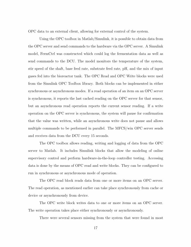
OPC data to an external client, allowing for external control of the system.

Using the OPC toolbox in Matlab/Simulink, it is possible to obtain data from

the OPC server and send commands to the hardware via the OPC server. A Simulink

model, FermCtrl was constructed which could log the fermentation data as well as

send commands to the DCU. The model monitors the temperature of the system,

stir speed of the shaft, base feed rate, substrate feed rate, pH, and the mix of input

gases fed into the bioreactor tank. The OPC Read and OPC Write blocks were used

from the Simulink OPC Toolbox library. Both blocks can be implemented in either

synchronous or asynchronous modes. If a read operation of an item on an OPC server

is synchronous, it reports the last cached reading on the OPC server for that sensor,

but an asynchronous read operation reports the current sensor reading. If a write

operation on the OPC server is synchronous, the system will pause for confirmation

that the value was written, while an asynchronous write does not pause and allows

multiple commands to be performed in parallel. The MFCS/win OPC server sends

and receives data from the DCU every 15 seconds.

The OPC toolbox allows reading, writing and logging of data from the OPC

server to Matlab. It includes Simulink blocks that allow the modeling of online

supervisory control and perform hardware-in-the-loop controller testing. Accessing

data is done by the means of OPC read and write blocks. They can be configured to

run in synchronous or asynchronous mode of operation.

The OPC read block reads data from one or more items on an OPC server.

The read operation, as mentioned earlier can take place synchronously from cache or

device or asynchronously from device.

The OPC write block writes data to one or more items on an OPC server.

The write operation takes place either synchronously or asynchronously.

There were several sensors missing from the system that were found in most

17

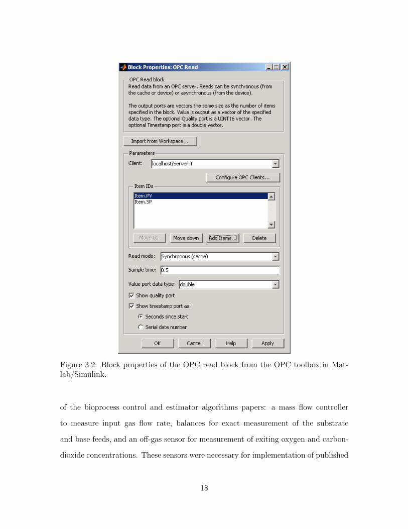
Figure 3.2: Block properties of the OPC read block from the OPC toolbox in Mat-lab/Simulink.

of the bioprocess control and estimator algorithms papers: a mass flow controller

to measure input gas flow rate, balances for exact measurement of the substrate

and base feeds, and an off-gas sensor for measurement of exiting oxygen and carbon-

dioxide concentrations. These sensors were necessary for implementation of published

18

Figure 3.3: Block properties of the OPC write block from the OPC toolbox in Mat-lab/Simulink.

methods and development of new ones, but the Biostat B DCU was unable to integrate

these new signals into the MFCS/win OPC data stream.

The mass flow controller (Omega Engineering Inc., Stamford, CT) was added

to control the flow of gas into the bioreactor. The mass flow controller is controlled

via an analog voltage input directly mapped to flow rate: 0 − 5V → 0 − 10L/min.

An onboard digital display allows confirmation of set mass flow rate. The voltage

is supply via a Quanser Q4 board connected to a computer running xPC Target.

xPC Target is a Mathworks product that loads in place of the operating system and

19

executes a compiled Simulink model. In this case, the Simulink model implemented

monitors the Ethernet port for commands via user datagram protocol (UDP), which

is a networking protocol that doesn’t require a handshake to establish a connection

or any confirmation from the receiver to transmit a package. A UDP block in the

FermCtrl model sets the desired flow rate set-point and receives the flow rate data.

The UDP block is set to send/receive data every 5 seconds.

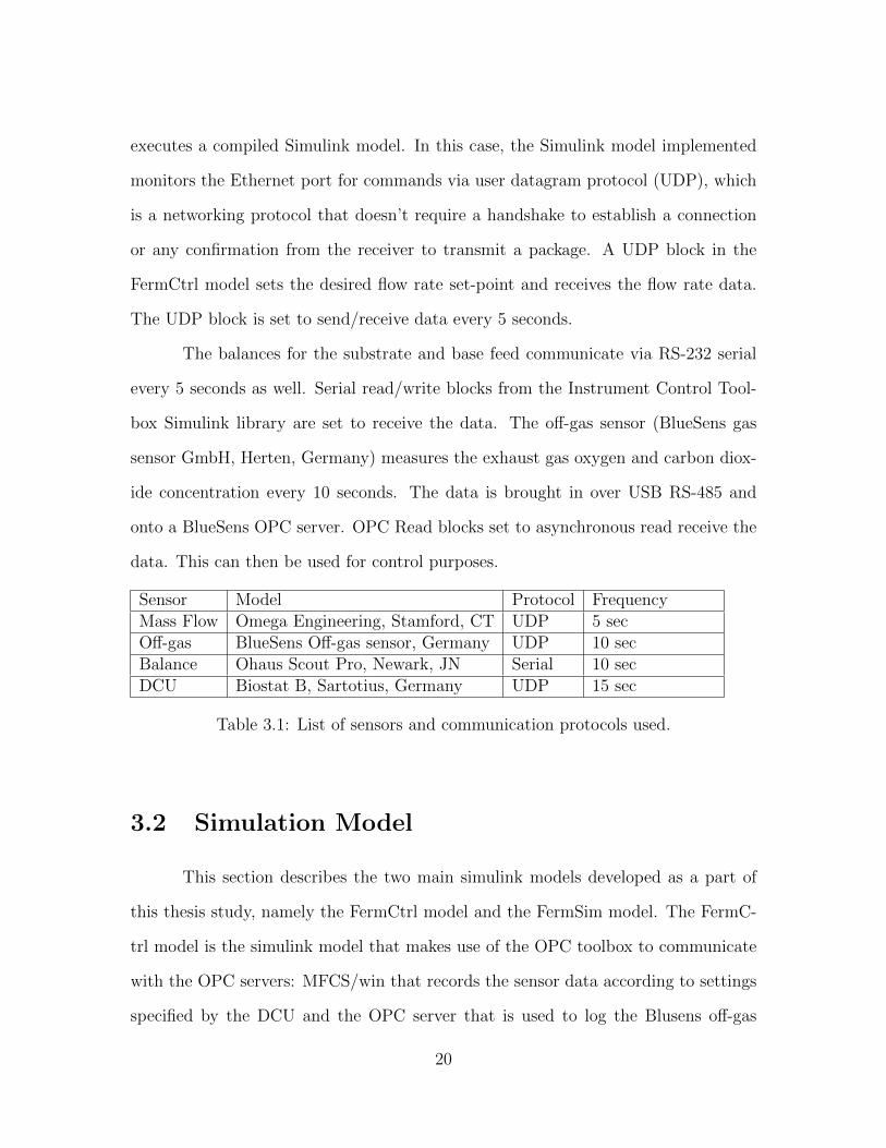
The balances for the substrate and base feed communicate via RS-232 serial

every 5 seconds as well. Serial read/write blocks from the Instrument Control Tool-

box Simulink library are set to receive the data. The off-gas sensor (BlueSens gas

sensor GmbH, Herten, Germany) measures the exhaust gas oxygen and carbon diox-

ide concentration every 10 seconds. The data is brought in over USB RS-485 and

onto a BlueSens OPC server. OPC Read blocks set to asynchronous read receive the

data. This can then be used for control purposes.

Sensor Model Protocol FrequencyMass Flow Omega Engineering, Stamford, CT UDP 5 secOff-gas BlueSens Off-gas sensor, Germany UDP 10 secBalance Ohaus Scout Pro, Newark, JN Serial 10 secDCU Biostat B, Sartotius, Germany UDP 15 sec

Table 3.1: List of sensors and communication protocols used.

3.2 Simulation Model

This section describes the two main simulink models developed as a part of

this thesis study, namely the FermCtrl model and the FermSim model. The FermC-

trl model is the simulink model that makes use of the OPC toolbox to communicate

with the OPC servers: MFCS/win that records the sensor data according to settings

specified by the DCU and the OPC server that is used to log the Blusens off-gas

20

sensor measurement data as shown in Figure 4.1. It is a hardware-in-the-loop im-

plementation with the FermSim simulink model setup in parallel to the OPC read

blocks that provide online sensor information from the physical hardware setup, with

the ability to switch between the two. The FermSim simulink model contains the Xu

uptake rate model described by the ODEs in Equation 2.4. The model also contains

an estimator to calculate oxygen uptake rate [3] from the Bluesens O2 measurements

and simulated feed profiles that can be varied to match the experimental feed profiles

accurately. In addition, certain other features of these models are discusses in this

section in some detail.

3.2.1 FermCtrl Model

The purpose of the FermCtrl model is to implement previously published or

new bioprocess control and estimator algorithms. The development of these algo-

rithms was sped up by creating a simulation environment that could mimic the dy-

namics of the culture, the bioreactor system, and all the sensors. In the first few

experiments, the FermCtrl model was used to record data while the MFCS/win and

DCU controlled the fermentation. The recorded data is used for sensor and E. coli

culture characterization. The fundamental sample time of the FermCtrl model is set

to 5 seconds and all commands and data are recorded in a .mat file. During later

experiments, FermCtrl was used to take control of sensors from the DCU if needed.

The FermCtrl model behaves as a switch between the simulated platform,

where the bioprocess is modeled based on mathematical equations and the physical

hardware system where data is logged to the OPC server from various on-line sensors.

This hardware-in-the-loop approach allows the development and testing of control

strategies of high complexity in a fast and accurate manner, with the added benefit

21

of not straining expensive equipment. Simulation systems offer a way for control to

be implemented and tested with regards to efficiency and safety, before porting it to

the physical system.

Another advantage of developing such a setup is that numerous tests can be run

in a short period of time while conserving material required for actual experimental

runs, which also limits waste production.

3.2.2 FermSim Model

The simulation platform, called FermSim, allows testing of control algorithms

at a much faster pace when compared to testing it on the physical system. The

FermSim parameters are improved by taking experimental results and fitting the

simulation parameters to fit the data recorded. By doing this, it is possible to model a

simulation as closely as possible to the actual system. The FermSim model developed

for this study is an extension of the Xu model, discussed in earlier chapters of this

thesis. This section describes the FermSim model used to model culture behavior on

simulink.

The FermSim model consists of a growth rate block that contains all the ODEs

that make up the Xu model. It has been developed in a way that makes it convenient

to change the culture model as required. Another feature of the FermSim model is

its initialization file, where all the initial values related to a particular experimental

run/strain type can be specified. The model allows custom feed profiles to be input,

and can also accept feed profiles directly in the form of a .mat file for both substrate

and base feed. This allows reusability while running different characterization ex-

periments and allows the same model to be extended for the parameter fitting using

numerical minimization algorithms. In addition, the model has the capacity to accept

22

both discreet and continuous feed profiles, allowing some flexibility with regards to

feed profiles for different control strategies. The stir control block is located outside

the bioreactor block, and can be housed with application specific stir control logic.

A separate block for OUR estimation is also provided to allow different estimator

logics to compute OUR in real time, again based on application needs. The model is

developed to run in both hours and seconds and can be switched between one and the

other. By designing it in this way, it is possible to use different estimators or control

blocks depending on the time step they are configured to. The robustness of this

model makes it ideal for estimation and parameter estimation purposes. In Figure

3.5, the separate modules are represented. Each block contains the ODEs required to

calculate parameters required for the modeling of the E. coli metabolic bioprocess.

3.2.3 OUR Estimator

Sensor dynamics are modeled to obtain a filtered OTR value. This OTR is

then used for the computation of OUR. The OUR estimator [3] makes use of qO,

which is an output of the growth rate block, to determine OUR of the culture at a

given point in time. The volumetric oxygen transfer coefficient kLa can be calculated

by the following equation:

kLa = a0 + a1(N −N0) (3.1)

This equation implies that there is an almost linear relationship between kLa

and stir speed N . The constants a0, a1 and N0 are system/strain specific and are

obtained from the initialization files. Subsequently, the kLa is used to calculate the

23

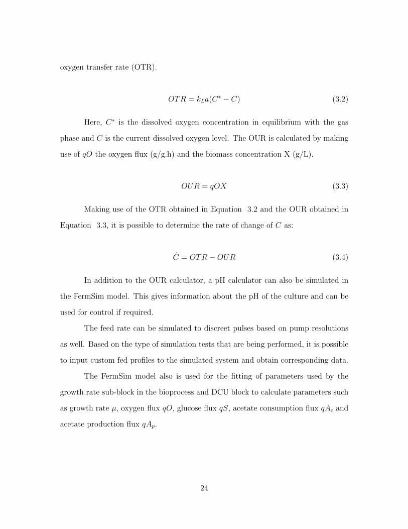
oxygen transfer rate (OTR).

OTR = kLa(C∗ − C) (3.2)

Here, C∗ is the dissolved oxygen concentration in equilibrium with the gas

phase and C is the current dissolved oxygen level. The OUR is calculated by making

use of qO the oxygen flux (g/g.h) and the biomass concentration X (g/L).

OUR = qOX (3.3)

Making use of the OTR obtained in Equation 3.2 and the OUR obtained in

Equation 3.3, it is possible to determine the rate of change of C as:

C = OTR−OUR (3.4)

In addition to the OUR calculator, a pH calculator can also be simulated in

the FermSim model. This gives information about the pH of the culture and can be

used for control if required.

The feed rate can be simulated to discreet pulses based on pump resolutions

as well. Based on the type of simulation tests that are being performed, it is possible

to input custom fed profiles to the simulated system and obtain corresponding data.

The FermSim model also is used for the fitting of parameters used by the

growth rate sub-block in the bioprocess and DCU block to calculate parameters such

as growth rate µ, oxygen flux qO, glucose flux qS, acetate consumption flux qAc and

acetate production flux qAp.

24

3.3 Configuring Simulation Models

3.3.1 Configuring FermCtrl

FermCtrl makes use of OPC read/write blocks to obtain online data logged in

the OPC server and send commands to the DCU during the course of the fermenta-

tion. The OPC blocks require the group ID of the reactor it is communicating with,

as well as the tags for each of the variables it reads from or writes to. The FermCtrl

model can also be used to set the control mode and control status of each of the

online sensors with the OPC write blocks. A user interface was created to allow easy

access to sensor settings and values as shown in Figure 3.4.

The OPC data read from the server is logged to a destination .mat file. Switch-

ing the group ID tags of the OPC read/write blocks to the simulation server allows the

FermSim model to run and log data onto the .mat file instead. In this way, FermCtrl

acts as a switch between the simulation model and the hardware platform.

3.3.2 Configuring FermSim

For FermSim to run, the .mat file containing the initial values needs to be set

up. This initialization file contains all the starting values specific to a fermentation

run, including the initial volume in the bioreactor tank, the initial acetate and glucose

levels obtained as offline samples and the other constants used in the FermSim model.

The full list of initial values is available in the appendix. The type of feed profile being

used also needs to be specified. The FermSim model is capable of accepting a purely

simulated feed profile or an actual experimental feed profile in the form of a .mat

file. The feed can also be discreet pulses or a continuous curve. For the fitting

of parameters which is described in greater detail in the next chapters, the actual

25

Figure 3.4: User Interface developed along with FermCtrl for easy read/write accessof the OPC server variables.

experimental feed profile is used for both glucose and base feeds. There are three

inputs to the FermSim simulation model; the stir speed N , the base feed rate Fb and

the substrate feed rate Fs. The important output variables of FermSim simulation

model are growth rate µ, acetate concentration A, glucose concentration S, biomass

concentration X, oxygen uptake rate OUR and base and substrate balance values.

All output values are logged to a .mat file for the entire duration of the experiment,

along with the simulated culture time.

26

Figure 3.5: Representation of the Simulink model FermSim along with the input andoutput variables.

The initialization file, called FermSim.mat is experiment specific and is loaded

to the simulink workspace before the start of the simulation, for access by FermSim.

This allows the same simulation model to be used for all experimental runs, while

only requiring the appropriate initialization files and feed profile .mat files.

27

Chapter 4

Experimental Procedure

This chapter descries the experimental procedure used to perform the E. coli

fermentation process and log the output data. It also includes information about the

offline sampling protocol.

4.0.3 E. coli Fermentation Procedure

For the purpose of gathering data of typical E. coli fermentation runs, deter-

mining sensor delays and system response times, characterization experiments were

performed on E. coli strain MG1655. This section presents a typical experimental

run along with a description of the procedure. Figure 4.1 shows the overall setup of

the bioreactor and the related sensors.

The experimental hardware setup is shown in Figure 4.1. The experiment

begins with the prepping of the fermenter and positioning of probes and stir blades

in the required manner. The sensors are calibrated if needed and primed in the

case of the pumps. An overnight culture is introduced into the bioreactor tank after

the initial OD measurement is recorded. The feed profile is predetermined and the

control is handed to the DCU. The mass flow level is set to the desired level and other

28

Figure 4.1: Experimental setup of the bioreactor and related sensors. 1: Glucosebalance; 2: Glucose bottle; 3: Bioreactor vessel; 4: DO probe; 5: Stir motor; 6: pHprobe; 7: Base balance; 8: Base bottle; 9: Mass flow controller; 10: DCU pumps (topto bottom - acid, glucose, antifoam, base); 11: Bluesens off-gas sensor; 12: DCU; 13:xPC target. [3]

additives such as IPTG are introduced into the bioreactor tank when required.

The fermentation process itself consists of two phases, the batch phase and the

fed-batch phase. During the batch phase, the cells consume the glucose that is initially

present in the bioreactor and rapidly grow. After all the glucose is depleted, the cells

start to feed on the acetate, usually indicated by a sudden spike in the dissolved

29

oxygen level; this marks the end of the batch phase. In fed-batch phase, glucose is

fed using an open-loop exponential feed profile or a controlled custom profile. During

the fed-batch phase, after the cells reach a predetermined density, chemicals such as

isopropyl-beta-thiogalacosidase (IPTG), are added that induce the cells to make the

product, usually recombinant proteins [28].

Sampling is done every half an hour and provides the off-line measurements of

glucose, OD and acetate levels, which are not obtainable by on-line sensor measure-

ments. During the sampling process, a 1.5 mL sample is taken out of the bioreactor.

This sample is used to measure the OD level and then spun down using a centrifuge

to remove the bio-material and the remaining liquid is frozen. Once the experiment

is complete, the frozen samples are thawed out and used to check for the glucose

and acetate levels respective to their sample times. This gives an estimate of the

acetate concentration and glucose concentration in the culture during the sampled

times. The experiment consists of a batch phase and a fed-batch phase. Typically,

the drop in the dissolved oxygen (DO) levels indicates the end of batch phase and

the start of fed-batch phase. For the E. coli strain used in these experiments, this

typically occurs at 5-6 hours culture time.

The plots for on-line measurements and offline measurements of a typical fer-

mentation run with non-induced E. coli is shown in Figure 4.3 and Figure 4.2.

The glucose concentration and acetate concentration measurements in Figure 4.3 are

offline measurements and the rest of the plots are obtained from on-line sensors.

30

Figure 4.2: A plot of DO (percent), Stir speed (rpm), pH, Temperature (degree C)and Mass flow (L/min) versus Time(h).

31

Figure 4.3: A plot of O2 (percent), Glucose balance reading (g), Base balance read-ing (g), Acetate concentration offline measurement (g/L) and Glucose concentrationoffline measurement (g/L) versus Time (h).

32

Chapter 5

Experimental Results

This chapter presents the results of the parameter estimation algorithm along

with the errors observed while fitting using numerical minimization. This chapter

also presents the methodology incorporated for parameter estimation by the means

of numerical minimization and offers comparison to values used in the original Xu

model [2].

5.1 Numerical Minimization

The obtained results are compared to the performance of the original growth

block parameters obtained from the Xu model [2].

qOs ≤ qOmax/(1 + A/Ki,O) (5.1)

The half rate consumptions for glucose uptake and acetate consumption are

Monod terms described in the Equations 2.5 and 2.9. Ki,S represents the inhibition

term in Equation 2.5 and Ki,O is the boundary condition term in Equation 5.1.

KA and KS are empirical coefficients to the Monod equation, and are E. coli strain

33

Variable (units) DescriptionKA (g/L) Half rate Acetate Consumption, Monod termKi,O (g/L) OUR inhibition by AcetateKi,S (g/L) GUR inhibition by AcetateKS (g/L) Half rate Glucose Uptake, Monod termqACmax (g/Lhr.) max Acetate Consumptionqm (g/Lhr.) maintenanceqOmax (g/Lhr.) max OURqSmax (g/Lhr.) max GURYA/S (g/g) g A produced per g S, Stoichiometric constantYO/A (g/g) g O consumed per g A, Stoichiometric constantYO/S (g/g) g O consumed per g S, Stoichiometric constantYX/A (g/g) g X produced per g AYX/Sof

(g/g) g X produced per g S, during overflow metabolismYX/Sox (g/g) g X produced per g S, during oxidative metabolism

Table 5.1: Estimation parameter description.

specific. The half rate acetate consumption is set to 0.05 and the half rate glucose

consumption is set to 0.05 [2].

YA/S, YO/A and YO/S are stoichiometric constants [2]. Ki,O, Ki,S, qACmax , qm,

qOmax, qSmax, YX/A, YX/Sofand YX/Sox are the fitted to three training experiment

datasets obtained by the procedure described in Chapter 4.0.3, for three seperate

feed profiles and initialization files. They are verified against a fourth experimentally

obtained dataset that is not used for training. The constraints and stopping con-

ditions of the numerical minimization method determines the accuracy of the fitted

parameters.

5.1.1 Minimization Procedure

For the process of parameter estimation of the fermentation model, experi-

mentally obtained datasets from three different experiments are used as training data

sets. The data is fed into a Simulink script that runs the FermSim model iteratively,

34

in an attempt to form a Gaussian and determine the best fit for the selected parame-

ters, based on tolerance conditions and iteration limits. Constrained minimization is

performed and the algorithm makes use of an objective function to determine the er-

ror between the simulated data and the experimentally recorded data. The Simulink

function used for this is fmincon. Constraints are set on the upper and lower bounds

of the parameter values. The bounds ensure that the minimization does not try to

fit to impossible parameter values like values less than zero. The algorithm is not

constrained with regards to number of iterations or maximum function evaluations.

Tolerances are set for the parameter values, represented as unknowns x and the min-

imization or objective function error, fval.

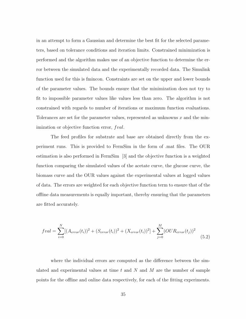
The feed profiles for substrate and base are obtained directly from the ex-

periment runs. This is provided to FermSim in the form of .mat files. The OUR

estimation is also performed in FermSim [3] and the objective function is a weighted

function comparing the simulated values of the acetate curve, the glucose curve, the

biomass curve and the OUR values against the experimental values at logged values

of data. The errors are weighted for each objective function term to ensure that of the

offline data measurements is equally important, thereby ensuring that the parameters

are fitted accurately.

fval =N∑i=0

[(Aerror(ti))2 + (Serror(ti))

2 + (Xerror(ti))2] +

M∑j=0

(OURerror(tj))2

(5.2)

where the individual errors are computed as the difference between the sim-

ulated and experimental values at time t and N and M are the number of sample

points for the offline and online data respectively, for each of the fitting experiments.

35

Each training dataset produces a fval and the sum of these fval forms the overall

objective function’s Fval. This ensures that a best fit across all training experiments

is obtained, as total fval is a sum of individual Fvals. Figure 5.1, Figure 5.2 and

Figure 5.3 are the three training dataset plots and Figure 5.4 is the verification plot.

Each point represents a recorded data point. In the case of acetate concentration

A, substrate concentration S and biomass concentration X, these are offline sampled

data. In the case of OUR, it is the data logged by the BlueSens in its OPC server.

Each experiment has its own initialization file, feed profile and sampling fre-

quency. In the case of the first training experiment, offline samples were recorded

every hour, whereas in the case of the other two training experiments and the verifi-

cation experiment, offline samples were recorded every half an hour. The developed

procedure allows for this sort of staging. The appropriate initial conditions file, feed

profiles and sampling information are used by the respective experiment numbers.

Using the experimental conditions and feed in the simulation ensures near identical

conditions for the simulated environment. Each of the files are read directly from

Matlab’s workspace during the iterative minimization process and need to be loaded

and cleared in succession for each iteration. Any number of training datasets can

be added as the setup is very scalable. The initial guess for this minimization was

varied and the final result obtained is verified to be a true minimum, for the given

constraints. The reason the process is performed multiple times with different initial

guesses is to ensure the minimization is returning a true global minimum, and not a

local minimum.

The error associated with each term in the overall Fval function determines

the degree of fitting to each individual experiment. Further, each of these fval terms

consist of the error values due to A, S, X, and OUR. Each of these error values in the

fval expression are weighed differently, according to the error magnitude observer. To

36

Figure 5.1: Training experiment 1 plots for A, S, X and OUR using fitted parameters.

compare the fitting results with the original Xu parameter values [2], the maximum

error associated for each of the objective function curves (A, S, X and OUR) is

observed. Table 5.2 shows the minimization result value and the Xu value for each

37

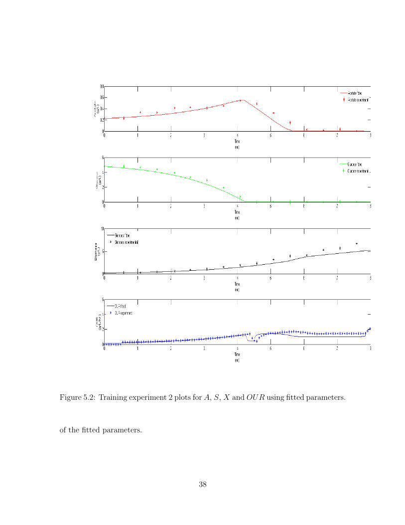
Figure 5.2: Training experiment 2 plots for A, S, X and OUR using fitted parameters.

of the fitted parameters.

38

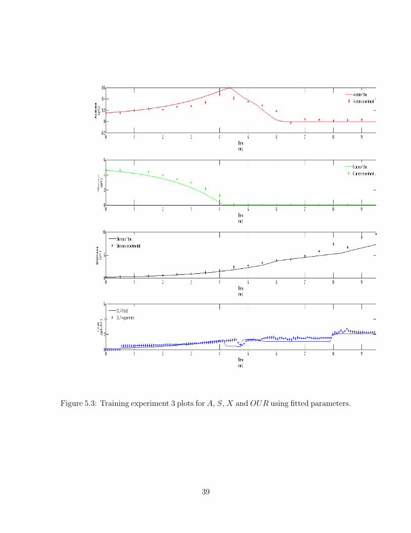
Figure 5.3: Training experiment 3 plots for A, S, X and OUR using fitted parameters.

39

Variable (units) Xu Value Fitted ValueKi,O (g/L) 4.0000 6.999762102368000Ki,S (g/L) 5.0000 8.689703450900000qACmax (g/Lhr.) 0.2000 0.236917644789370qm (g/Lhr.) 0.0400 0.069879903886394qOmax (g/Lhr.) 0.4290 0.750040424418578qSmax (g/Lhr.) 1.2500 1.592771481184673YX/A (g/g) 0.4100 0.090888556829738YX/Sof

(g/g) 0.1510 0.270537251296590YX/Sox (g/g) 0.5110 0.401978605025204

Table 5.2: Growth block parameter numerical minimization best fit values.

5.2 Fitting Limitations

The fitted parameter results depend on many factors. The most important

factor that affects the fitting results is the number of offline sample points available

to fit against. The frequency of sampling for the first training experiment is once

every hour, and the sampling rate for the other two training experiments is every

half an hour. This directly affects the fitting results. The OUR data is available

at 5 second intervals which is the sample time set in the BlueSens OPC server for

logging frequency. This is an online measurement. The individual curves need to be

weighed according to the sample frequency and the magnitude of change observed

between data points. Another limitation is with the measurement of acetate and

glucose concentration levels from the offline samples. As discussed in Section 4.0.3,

the sampled biomaterial is spun down and the solid biomaterial is discarded and the

remaining solution is frozen for analysis. In the case of glucose a YSI 2900 meter

is used to measure concentration. Depending on the type of membrane used in the

YSI, corresponding levels of accuracy can be seen in the offline glucose concentration

measurements. The YSI membrane available in the lab has a precision of 0.02(g/L)

40

with an accuracy of ±2%. In the case of acetate concentration measurements, an

acetate assay kit is used. Kit A0504−85 by BioAssay is the acetate assay kit available

in the lab. The acetate assay kit uses enzyme-coupled reactions to form colored,

fluorescent product. The detection range of this kit is 0.20 − 20mM acetate for

colorimetric assays and 0.13− 2.0mM for fluorimetric assays. The colorimetric assay

measures the change in light absorption while the flourimetric assay uses difference

in fluorescence of substrate. For the simulation to switch from overflow metabolism

to oxidative metabolism at the end of batch phase, it is essential that zero acetate

concentration levels are detected in the fermentation. The accuracy of measurement

can affect this condition and can result in the simulation remaining in overflow longer

than it should be.

5.3 Result Analysis

The verification dataset is fitted with the minimization parameters and the

results can be seen in Figure 5.4. The same experiment is plotted for, using the Xu

parameters for comparison Figure 5.5.

To compare the performance of the simulation while using the fitted param-

eters versus the Xu parameters, the errors associated with each of the four terms of

the objective function can be compared as seen in Table 5.3. The root mean square

errors of each of the curves in the objective expression for the verification experiment

is also shown in Table 5.3.

Parameters Used Acetate Error Glucose Error Biomass Error OUR ErrorXu Parameters 4.87 6.68 20.15 8.74Fitted Parameters 2.35 3.55 12.85 5.88

Table 5.3: Error comparison for Fitted vs Xu parameters for the verification experi-ment.

41

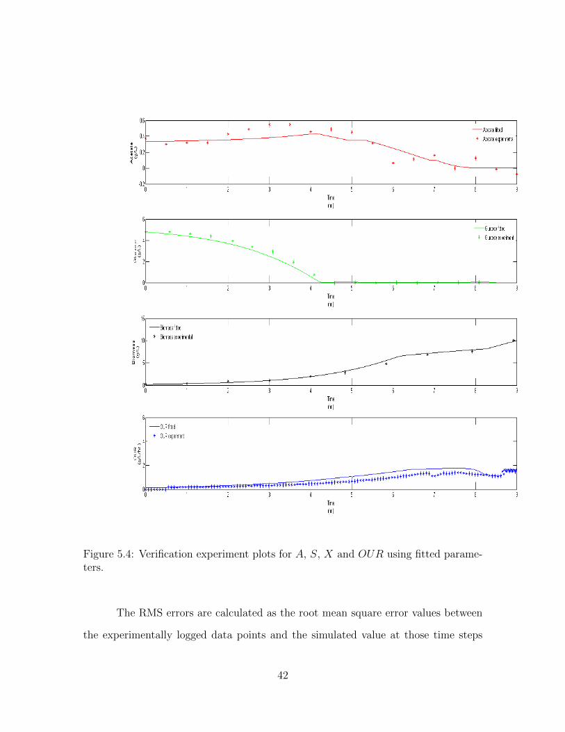
Figure 5.4: Verification experiment plots for A, S, X and OUR using fitted parame-ters.

The RMS errors are calculated as the root mean square error values between

the experimentally logged data points and the simulated value at those time steps

42

Figure 5.5: Verification experiment plots for A, S, X and OUR using Xu parameters.

for each of the curves used in the objective function expression, A, S, X and OUR.

The RMS errors for the fitter parameters are computed for the verification experiment

and compared to the original Xu parameters [2] for the same verification experiment.

43

This gives a clear metric to compare the performance between the fitted parameters

and the original Xu parameters.

The errors in Table 5.3 do not include the weight terms specified in Table

5.4. For this minimization, the weights associated with each term are shown in Table

5.4.

Fitting Term WeightAcetate Concentration 1500Glucose Concentration 20Biomass Concentration 20OUR 1

Table 5.4: Objective function weights for each term.

The reason for large Biomass error is that the value of X is exponentially

increasing with increasing culture time and so, to accurately account for all terms in

Equation 5.2, the terms are given their respective error weights. OUR error values are

also large because of the number of sample points available to fit to. This is because

the off-gas sensor used to record OUR data is an online sensor that records data every

5 seconds, throughout the fermentation process as compared to offline measurements

A, S and X which are recorded only every half an hour in the case of the verification

experiment used in this thesis. The acetate weight is the highest as for most of the

batch phase, there is acetate present in the system but the fed batch typically is

started when most of the acetate is consumed during the metabolite consumption

phase. Therefore, it is of critical importance to accurately fit to this drop in the

acetate level as the simulation will exit overflow only when the acetate level in the

system is zero. There is significant emphasis given to fitting biomass correctly, as

the simulation needs to be able to accurately fit biomass for it to be a viable means

to test control strategies. As discussed in Section 1.1. The original Xu model has

44

trouble fitting acetate concentration A. The fitted parameters in comparison perform

significantly better. This, along with the addition of OUR as a sensor for which data

can be logged online and fitted to, makes the simulation model more precise as there

are more data points to fit to. OUR is also a good indicator of metabolic activity, in

combination with A, S and X.

45

Chapter 6

Conclusion and Future Work

The design and implementation of simulation platforms for modeling and pa-

rameter estimation of E. coli metabolism is presented in this thesis. The process of

numerical minimization is also described. The combination of these two simulation

models allows for a combined setup that can effectively allow for dynamic parameter

estimation and control strategy testing.

6.0.1 Conclusion

The FermCtrl model is used for hardware-in-the-loop implementation of the

physical hardware system that communicates with the simulation using Matlab’s

OPC toolbox. It is possible to log data from the OPC server as well as write values

to the various sensors controlled by the DCU. This is able to run in-tandem with

the FermSim model which is a simulated model that is used to replicate the behavior

of the physical hardware setup. The combination of these systems offers a complete

platform to test and configure fermentation control protocols and verify results in an

accurate and fast manner effectively. The FermCtrl model is able to interact with the

DCU with the use of OPC read/write blocks and the system can be used to effectively

46

take over all control of sensors from the DCU and allows control to be handed over

to a remote system with the help of simulink.

The FermSim model is able to reliably display expected bioprocess behavior

extremely quickly. A typical fermentation run that can take 12-20 hours is simulated

in a matter of seconds and with the implementation of parameter fitting, it is possible

to accurately observe trends and implement control strategies. The combination of

the FermSim model for development and the FermCtrl model for testing makes this

a very useful system. With many different strains of E. coli being developed, it is

important to tune the simulation system to the behavior of that strain. With the Xu

model, data sets from only a few experiments can fit pre- and post-induction behavior

for a strain. This is made possible using the numerical minimization algorithm, in

conjuction with the FermSim model. E. coli strains with the different plasmids and

even the same strains with different amounts of IPTG can have drastically different

behavior [8, 28]. Once the strain has been characterized, work can begin on different

estimator and control designs. The FermSim model is able to compare different test

control strategies as well as equate them to published algorithms. By conventional

means, it is hard to compare algorithms implemented using different strains and with

different experimental conditions. The development of the described model makes

this easy to implement.

6.0.2 Future Work

It is possible to use the same overall structure and add additional estimators

to improve simulation behavior and more effectively capture metabolic activity. This

can lead to additional terms in the objective function which can improve the fitting

of parameters further. Different fermentation experiments can be be simulated by

47

making the necessary changes to the bioreactor block. FermSim has been developed in

a multi-level format that allows simplified swapping in and out of required blocks with

a variable tagging architecture. This means that the required variables or constant

parameters need to be altered in only one location in the model and the updated

version is carried to all levels of the simulated model including all sub-blocks by

the means of reference tags. This makes it very convenient to make changes and

test various fitting strategies and control methods. Additionally, this will also allow

similar parameter estimation and control strategy testing to be run for various other

bioprocesses as only the relevant tags need to be altered accordingly.

48

Appendices

49

Appendix A FermSim Model

Figure 1: Simulink model FermSim with input and output variables.

The simulink model is embedded in an outer model which also includes the

50

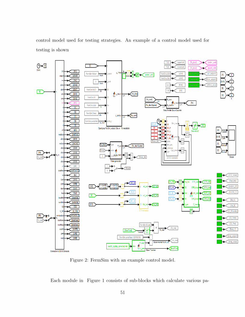
control model used for testing strategies. An example of a control model used for

testing is shown in Figure ??.

Figure 2: FermSim with an example control model.

Each module in Figure 1 consists of sub-blocks which calculate various pa-

51

rameters used to simulate culture metabolism. The matlab workspace contains infor-

mation of all the initial values which are experiment specific. A full list of variables

in the initialization file can be seen in Table 1. A typical sub-module is shown in

Figure 3.

Figure 3: The S sub-module block.

The initial values are stored in a .mat file, FermSim.mat. This file also includes

a list of parameters that is currently being used by the growth rate block in the

52

FermSim model.

Variable Name (units) DescriptionexpDur (hr.) Duration of experimentfbStart (hr.) Fed-batch start timetScale (sec/hr.) Sec-to-hour conversionCstar (%) DO conc. in equilibriumC (%) Current DO levelN0 (rpm) Initial stir speed of motor shaftV0 (L) Initial volumeA0 (g/L) Initial acetate conc.S0 (g/L) Initial glucose conc.X0 (g/L) Initial biomass conc.PHset pH set pointbuffer (mM) Buffer molarityMasssubs(g) Initial glucose balance readingMassbase(g) Initial base balance readingXu Struct of all Xu parameters

Table 1: List of sensors and communication protocols used.

53

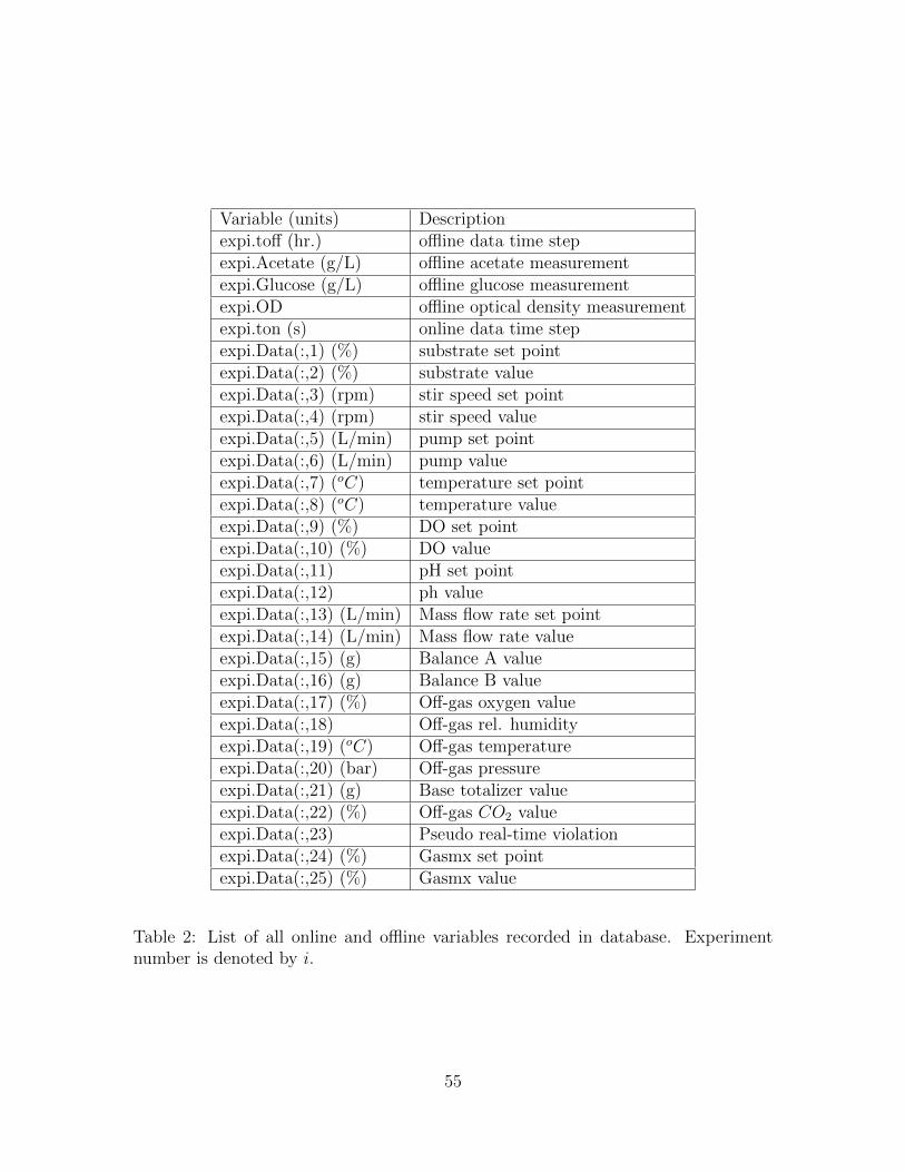
Appendix B Experiment Details

A single database with all offline and online variables was created for ease of

use during simulation and parameter minimization. The complete list of variables

associated are shown in Table 2. A total of ten experiments were performed with E.

coli and data for all ten experiments is available in the experiment database.

54

Variable (units) Descriptionexpi.toff (hr.) offline data time stepexpi.Acetate (g/L) offline acetate measurementexpi.Glucose (g/L) offline glucose measurementexpi.OD offline optical density measurementexpi.ton (s) online data time stepexpi.Data(:,1) (%) substrate set pointexpi.Data(:,2) (%) substrate valueexpi.Data(:,3) (rpm) stir speed set pointexpi.Data(:,4) (rpm) stir speed valueexpi.Data(:,5) (L/min) pump set pointexpi.Data(:,6) (L/min) pump valueexpi.Data(:,7) (oC) temperature set pointexpi.Data(:,8) (oC) temperature valueexpi.Data(:,9) (%) DO set pointexpi.Data(:,10) (%) DO valueexpi.Data(:,11) pH set pointexpi.Data(:,12) ph valueexpi.Data(:,13) (L/min) Mass flow rate set pointexpi.Data(:,14) (L/min) Mass flow rate valueexpi.Data(:,15) (g) Balance A valueexpi.Data(:,16) (g) Balance B valueexpi.Data(:,17) (%) Off-gas oxygen valueexpi.Data(:,18) Off-gas rel. humidityexpi.Data(:,19) (oC) Off-gas temperatureexpi.Data(:,20) (bar) Off-gas pressureexpi.Data(:,21) (g) Base totalizer valueexpi.Data(:,22) (%) Off-gas CO2 valueexpi.Data(:,23) Pseudo real-time violationexpi.Data(:,24) (%) Gasmx set pointexpi.Data(:,25) (%) Gasmx value

Table 2: List of all online and offline variables recorded in database. Experimentnumber is denoted by i.

55

Bibliography

[1] R. Jayaraj and P. Smooker, “So you need a protein - a guide to the productionof recombinant proteins,” Open Veterinary Science Journal, vol. 3, pp. 28–34,2009. [Online]. Available: http://www.bentham-open.org/pages/gen.php?file=28TOVSJ.pdf&PHPSESSID=f5293cfcd476d572c6840b8e34701e4a

[2] B. Xu, M. Jahic, and S. O. Enfors, “Modeling of overflow metabolism in batchand fed-batch cultures of escherichia coli,” Biotechnology progress, vol. 15, no. 1,pp. 81–90, Jan-Feb 1999.

[3] L. Wang, Master’s thesis, Clemson University, 2014.

[4] Y. Pomerleau and M. Perrier, “Estimation of multiple specific growth rates inbioprocesses,” AIChE Journal, vol. 36, no. 2, pp. 207–215, 1990.

[5] A. Rodriguez, G. Quiroz, J. D. Leon, and R. Femat, “State and parameter esti-mation of an anaerobic digester model,” in Automation Science and Engineering(CASE), 2011 IEEE Conference on, 2011, pp. 690–695.

[6] C. Diaz, P. Dieu, C. Feuillerat, P. Lelong, and M. Salome, “Adaptive predic-tive control of dissolved oxygen concentration in a laboratory-scale bioreactor,”Journal of Biotechnology, vol. 43, no. 1, pp. 21–32, Nov 21 1995.

[7] D. Levisauskas, R. Simutis, D. Borvitz, and A. Lbbert, “Automatic control ofthe specific growth rate in fed-batch cultivation processes based on an exhaustgas analysis,” Bioprocess Engineering, vol. 15, no. 3, pp. 145–150, Aug 1 1996.[Online]. Available: http://dx.doi.org/10.1007/BF00369618

[8] M. Akesson, P. Hagander, and J. P. Axelsson, “A probing feeding strategy forescherichia coli cultures,” Biotechnology Techniques, vol. 13, no. 8, pp. 523–528,Aug 1 1999.

[9] L. V., “On-line estimation of biomass concentration and non stationaryparameters for aerobic bioprocesses,” Journal of Biotechnology, vol. 46,no. 3, pp. 197–207, 1996. [Online]. Available: http://www.ingentaconnect.com/content/els/01681656/1996/00000046/00000003/art00197

56

[10] M. Akesson, P. Hagander, and J. P. Axelsson, “A pulse technique for controlof fed-batch fermentations,” in Control Applications, 1997., Proceedings of the1997 IEEE International Conference on, 1997, pp. 139–144.

[11] ——, “Avoiding acetate accumulation in escherichia coli cultures using feedbackcontrol of glucose feeding,” Biotechnology and bioengineering, vol. 73, no. 3, pp.223–230, May 5 2001.

[12] A. Vicente, J. I. Castrillo, J. A. Teixeira, and U. Ugalde, “On-line estimationof biomass through ph control analysis in aerobic yeast fermentation systems,”Biotechnology and bioengineering, vol. 58, no. 4, pp. 445–450, 1998.

[13] H. Valdes-Gonzalez and J. M. Flaus, “State estimation in a bioprocess describedby a hybrid model,” in Intelligent Control, 2001. (ISIC ’01). Proceedings of the2001 IEEE International Symposium on, 2001, pp. 132–137.

[14] H. Sang, F. Wang, D. He, Y. Chang, and D. Zhang, “On-line estimation ofbiomass concentration and specific growth rate in the fermentation process,”in Intelligent Control and Automation, 2006. WCICA 2006. The Sixth WorldCongress on, vol. 1, 2006, pp. 4644–4648.

[15] S. Tatiraju, M. Soroush, and R. Mutharasan, “Multi-rate nonlinear state andparameter estimation in a bioreactor,” in American Control Conference, 1998.Proceedings of the 1998, vol. 4, 1998, pp. 2324–2328 vol.4.

[16] D. Tingey, K. Busawon, and M. Saif, “Biomass concentration estimation usingthe extended jordan observable form,” in Control Applications, 2005. CCA 2005.Proceedings of 2005 IEEE Conference on, 2005, pp. 143–147.

[17] M. Keulers, “Structure and parameter identification of a batch fermentation pro-cess using non-linear modelling,” in American Control Conference, 1993, 1993,pp. 2261–2265.

[18] V. Ljubenova and M. Ignatova, “An approach for parameter estimation ofbiotechnological processes,” Bioprocess Engineering, vol. 11, no. 3, pp. 107–113,Aug 1 1994. [Online]. Available: http://dx.doi.org/10.1007/BF00369606

[19] V. N. Lubenova, “Stable adaptive algorithm for simultaneous estimation oftime-varying parameters and state variables in aerobic bioprocesses,” BioprocessEngineering, vol. 21, no. 3, pp. 219–226, Sep 1 1999. [Online]. Available:http://dx.doi.org/10.1007/s004490050667

[20] M. Perrier, S. F. de Azevedo, E. C. Ferreira, and D. Dochain, “Tuning of observer-based estimators: theory and application to the on-line estimation of kineticparameters,” Control Engineering Practice, vol. 8, no. 4, pp. 377–388, Apr 2000.

57

[21] G. Bastin and D. Dochain, On-line Estimation and Adaptive Control of Biore-actors. Amsterdam, Netherlands: Elsevier Science, 1990.

[22] A. Johnson and S. Goody, “The original michaelis constant: Translation of the1913 michaelismenten paper,” American Chemical Society, vol. 50, no. 39, p.82648269, 09 2011.

[23] A. J. Wolfe, “The acetate switch,” Microbiology and Molecular BiologyReviews, vol. 69, no. 1, pp. 12–50, Mar 2005. [Online]. Available:http://dx.doi.org/10.1128/MMBR.69.1.12-50.2005

[24] V. Lubenova, I. Rocha, and E. C. Ferreira, “Estimation of multiple biomassgrowth rates and biomass concentration in a class of bioprocesses,” Bioprocessand Biosystems Engineering, vol. 25, no. 6, pp. 395–406, July 1 2003. [Online].Available: http://dx.doi.org/10.1007/s00449-003-0325-1

[25] C. Karakuzu, M. Turker, and S. Ozturk, “Modelling, on-line state estimation andfuzzy control of production scale fed-batch baker’s yeast fermentation,” ControlEngineering Practice, vol. 14, no. 8, pp. 959–974, Aug 2006.

[26] M. Pepper, “Designing a minimal-knowledge controller to achieve maximum sta-ble growth for an escherichia coli bioprocess,” Ph.D. dissertation, Clemson Uni-versity, June 2013.

[27] G. L. Kleman, K. M. Horken, F. R. Tabita, and W. R. Strohl, 1996.

[28] R. G. Harrison, P. Todd, S. Rudge, and D. P. Petrides, Bioseparations Scienceand Engineering. New York, New York: Oxford University Press, Inc., 2003.

58