modeling and optimization of tbcc engine performance
TRANSCRIPT

ABSTRACT
Title of Thesis: Modeling and Optimization of Turbine-Based
Combined-Cycle Engine Performance Joshua Clough, Master of Science, 2004 Thesis Directed By: Prof. Mark Lewis
Aerospace Engineering The fundamental performance of several TBCC engines is investigated from Mach 0-
5. The primary objective of this research is the direct comparison of several TBCC
engine concepts, ultimately determining the most suitable option for the first stage of
a two-state-to-orbit launch vehicle. TBCC performance models are developed and
optimized. A hybrid optimizer is developed, combining the global accuracy of
probabilistic optimization with the local efficiency of gradient-based optimization.
Trade studies are performed to determine the sensitivity of TBCC performance to
various design variables and engine parameters. The optimization is quite effective,
producing results with less than 1% error from optimizer repeatability. The turbine-
bypass engine (TBE) provides superior specific impulse performance. The
hydrocarbon-fueled gas-generator air turborocket and hydrogen-fueled expander-
cycle air turborocket are also competitive because they may provide greater thrust-to-
weight than the TBE, but require some engineering problems to be addressed before
being fully developed.
MODELING AND OPTIMIZATION OF TURBINE-BASED COMBINED-CYCLE
ENGINE PERFORMANCE
By
Joshua Clough
Thesis submitted to the Faculty of the Graduate School of the University of Maryland, College Park, in partial fulfillment
of the requirements for the degree of Master of Science
2004 Advisory Committee: Professor Mark Lewis, Chair Professor Christopher Cadou Professor Ken Yu

© Copyright by Joshua Clough
2004

PREFACE
“The existing technological ability and scientific background accumulated in many years of work will be lost if a small but continuing effort in this field is not maintained” -Antonio Ferri, speaking on the future of airbreathing engines at the 4th AGARD Colloquium, in 1960.
In the early 1960’s, NASA was working its way to the Moon, with the Apollo
program utilizing large rockets to accelerate humans to orbit by brute force and raw
power. These efforts, combined with the growing role of ICBMs in the US military,
seemingly spelled the end of advanced airbreathing engine research. Yet at the same
time, AGARD held its 4th colloquium, this time focusing on the science and research
behind high Mach number air breathing engines.
More than 40 years later, we are at a similar cross-roads, where grand
interplanetary programs are reducing (if not removing) funding from airbreathing
engine research. Yet the science behind these engines has not changed, and
airbreathing engines hold as much promise now as they did to Ferri that day in Milan.
ii

DEDICATION
To my grandfather, Poppy, who is part of the reason I am here today.
iii

ACKNOWLEDGEMENTS
This material is based upon work supported by a National Science Foundation
Graduate Research Fellowship. Additional support is provided by the Space Vehicles
Technology Institute, one of the NASA Constellation University Institute Programs,
under grant NCC3-989, with joint sponsorship from the Department of Defense.
Appreciation is expressed to Claudia Meyer of the NASA Glenn Research Center,
program manager of the University Institute activity, and to Drs. John Schmisseur and
Walter Jones of the Air Force Office of Scientific Research. The author would also
like to thank Dr. Ryan Starkey of the University of Maryland for the use of his GA
optimizer, Bonnie McBride of NASA Glenn Research Center for the use of CEA and
Tom Lavelle of NASA Glenn Research Center for his assistance with CEA and
engine modeling.
On a more personal level, many people aided me, both directly and indirectly,
in the completion of this work. I would like to thank my advisor, Mark Lewis, for his
guidance, encouragement, and support over the past two and a half years. I would
also like to thank Ryan Starkey for all of his help with Linux, optimization, locating
sources, and general advice regarding this thesis. I owe a good deal of my sanity over
the past years to my office-mates: Neal, Dan, Jesse, Justin, Andrew, Marc, Kerrie,
Dave, Amardip, Andy, Greg… thanks for everything. Finally, I would like to thank
my wife Ann for her amazing tolerance for “techno-babble”, putting up with my late
nights and early mornings, neck rubs, snacks, and support on every level. Thank you.
iv

TABLE OF CONTENTS Preface........................................................................................................................... ii Dedication .................................................................................................................... iii Acknowledgements...................................................................................................... iv Table of Contents.......................................................................................................... v List of Tables ............................................................................................................. viii List of Figures .............................................................................................................. ix List of Symbols ........................................................................................................... xii List of Acronyms ....................................................................................................... xiii Chapter 1: Introduction ................................................................................................. 1
1.1 Background................................................................................................... 1 1.1.1 RLV Concepts....................................................................................... 1 1.1.2 Airbreathing Engines ............................................................................ 1 1.1.3 Combined Cycle Engines...................................................................... 3
1.2 Project Description........................................................................................ 3 1.2.1 Motivation............................................................................................. 3 1.2.2 Objective ............................................................................................... 4
1.3 Previous Work .............................................................................................. 5 1.3.1 1913-1960: Early Ramjet and TBCC Development ............................. 5 1.3.2 1960-1990: Apollo, Cold War Era........................................................ 6 1.3.3 1990-Present: RLV Concepts for Access-to-Space .............................. 8 1.3.4 1990-Present: TBCC Engine Studies.................................................. 10 1.3.5 1990-Present: TBCC Engine Comparisons ........................................ 11
Chapter 2: Engine Cycles............................................................................................ 14 2.1 Brayton Cycle ............................................................................................. 14 2.2 Ramjet ......................................................................................................... 15
2.2.1 Flowpath ............................................................................................. 16 2.2.2 Operation............................................................................................. 16 2.2.3 Constraints .......................................................................................... 17
2.3 Turbojet....................................................................................................... 18 2.3.1 Flowpath ............................................................................................. 19 2.3.2 Operation............................................................................................. 20 2.3.3 Constraints .......................................................................................... 20
2.4 Turbine-Bypass Engine............................................................................... 21 2.4.1 Flowpath ............................................................................................. 22 2.4.2 Operation............................................................................................. 23 2.4.3 Constraints .......................................................................................... 24
2.5 Air Turborocket .......................................................................................... 25 2.5.1 Gas Generator ATR Flowpath ............................................................ 26 2.5.2 Expander-Cycle ATR Flowpath ......................................................... 27 2.5.3 Operation............................................................................................. 27 2.5.4 Constraints .......................................................................................... 29
Chapter 3: Engine Analysis ........................................................................................ 30
v

3.1 General Analysis......................................................................................... 30 3.2 Component Analysis................................................................................... 32
3.2.1 Inlet ..................................................................................................... 32 3.2.2 Fan/Compressor .................................................................................. 34 3.2.3 Turbine................................................................................................ 34 3.2.4 TBE Bypass Duct................................................................................ 35 3.2.5 Burner/Afterburner/Gas Generator ..................................................... 37 3.2.6 Expander ............................................................................................. 38
3.3 Assumptions................................................................................................ 39 Chapter 4: Engine Optimization ................................................................................. 41
4.1 Program Structure ....................................................................................... 41 4.2 Optimization ............................................................................................... 42
4.2.1 Gradient-Based Optimization ............................................................. 43 4.2.2 Probabilistic Optimization .................................................................. 47 4.2.3 Hybrid Optimization ........................................................................... 50 4.2.4 Objective Function.............................................................................. 51 4.2.5 Rubber Engine .................................................................................... 53
Chapter 5: Optimization Results................................................................................. 55 5.1 Input Conditions.......................................................................................... 55 5.2 TBE Trade Studies...................................................................................... 57
5.2.1 Bypass Ratio ....................................................................................... 57 5.2.2 Compressor Staging Ratio .................................................................. 64 5.2.3 Compressor Efficiency........................................................................ 69 5.2.4 Turbine Efficiency .............................................................................. 72 5.2.5 Fuel Inlet Temperature........................................................................ 74
5.3 GG-ATR Trade Studies .............................................................................. 77 5.3.1 Gas Generator Equivalence Ratio....................................................... 78 5.3.2 Turbine Efficiency .............................................................................. 82 5.3.3 Reactant Inlet Temperature................................................................. 86
5.4 EX-ATR Trade Studies............................................................................... 88 5.4.1 Fuel Inlet Temperature........................................................................ 89 5.4.2 Turbine Efficiency .............................................................................. 92 5.4.3 Chamber pressure................................................................................ 95
5.5 Engine Comparison..................................................................................... 98 5.5.1 Hydrocarbon-Fueled TBCC Comparison ........................................... 99 5.5.2 Hydrogen-Fueled TBCC Comparison .............................................. 102
5.6 Practical Implications of the Air Turborocket .......................................... 105 5.6.1 Turbine Separation / Power Transmission........................................ 106 5.6.2 Turbine-Compressor Balancing ........................................................ 108 5.6.3 EX-ATR Fuel Heating ...................................................................... 109 5.6.4 Engine Cooling ................................................................................. 109
5.7 “Non-rubber” engine performance ........................................................... 110 5.8 Summary ................................................................................................... 111
5.8.1 TBE................................................................................................... 111 5.8.2 GG-ATR ........................................................................................... 112 5.8.3 EX-ATR............................................................................................ 113
vi
5.8.4 Overall............................................................................................... 114 Chapter 6: Conclusions ............................................................................................. 115
6.1 TBCC Optimization and Comparison....................................................... 115 6.1.1 Compressor Exit Temperature Limit ................................................ 115 6.1.2 Ramjet Threshold.............................................................................. 115 6.1.3 TBCC Comparison............................................................................ 116 6.1.4 Assumed Parameter Sensitivity ........................................................ 118 6.1.5 Fuel Selection.................................................................................... 119
6.2 Accomplishments...................................................................................... 119 6.2.1 TBCC Performance Models.............................................................. 119 6.2.2 Hybrid Optimizer .............................................................................. 120 6.2.3 TBCC Performance Comparison ...................................................... 120
6.3 Future Work .............................................................................................. 121 References................................................................................................................. 123
vii

LIST OF TABLES Table 3.1: Assumed stoichiometric fuel ratios ........................................................... 40 Table 4.1: DOT non-default input parameters............................................................ 44 Table 4.2: GA non-default input parameters .............................................................. 49 Table 5.1: TBE bypass ratio trade study input parameters ......................................... 58 Table 5.2: TBE compressor efficiency values ............................................................ 70 Table 5.3: TBE turbine efficiency values ................................................................... 72 Table 5.4: GG-ATR equivalence ratio trade study input parameters ......................... 78 Table 5.5: EX-ATR fuel temperature trade study input parameters........................... 89 Table 5.6: TBCC engine comparison input parameters.............................................. 99
viii

LIST OF FIGURES
Figure 1.1: Specific Impulse as a function of Mach number for various engines1 ....... 2 Figure 1.2: Nord Aviation’s Griffon II TBCC-powered aircraft3 ............................... 6 Figure 1.3: Sketch of P&W J58 “bleed bypass” engine9 .............................................. 8 Figure 1.4: SAIC’s ICM-3 RLV concept12 ................................................................... 9 Figure 1.5: Boeing’s FASST concept13 ........................................................................ 9 Figure 2.1: Pressure-volume and temperature-entropy diagrams for the ideal Brayton
cycle26 ................................................................................................................. 14 Figure 2.2: Ramjet flowpath ...................................................................................... 15 Figure 2.3: Turbojet flowpath .................................................................................... 19 Figure 2.4: TBE flowpath ........................................................................................... 22 Figure 2.5: GG-ATR (bottom) and EX-ATR (top) flowpaths.................................... 26 Figure 3.1: Inlet diagram............................................................................................. 33 Figure 4.1: TBCC program flowchart......................................................................... 42 Figure 4.2: A comic representation of “hill-climbing” optimization33 ....................... 44 Figure 4.3: Graphical representation of constraint tolerance, courtesy of the DOT
User Manual33 ..................................................................................................... 45 Figure 5.1: Specific impulse vs. Mach for TBE with fixed and variable bypass ratios
............................................................................................................................. 58Figure 5.2: Thrust vs. Mach for TBE with fixed and variable bypass ratios............. 59 Figure 5.3: Bypass ratio vs. Mach for TBE with fixed and variable bypass ratios ... 59 Figure 5.4: Compressor ratio vs. Mach for TBE with fixed and variable bypass ratios
............................................................................................................................. 60Figure 5.5: Burner equivalence ratio vs. Mach for TBE with fixed and variable
bypass ratios........................................................................................................ 60 Figure 5.6: Afterburner equivalence ratio vs. Mach for TBE with fixed and variable
bypass ratios........................................................................................................ 61 Figure 5.7: Compressor inlet and exit temperature vs. Mach number for a
compression ratio of 1.1...................................................................................... 63 Figure 5.8: Specific impulse vs. Mach for TBE with fixed compressor staging ratios
............................................................................................................................. 65Figure 5.9: Thrust vs. Mach for TBE with fixed compressor staging ratios ............. 65 Figure 5.10: Bypass ratio vs. Mach for TBE with fixed compressor staging ratios .. 66Figure 5.11: Compressor ratio vs. Mach for TBE with fixed compressor staging
ratios.................................................................................................................... 66 Figure 5.12: Burner equivalence ratio vs. Mach for TBE with fixed compressor
staging ratios ....................................................................................................... 67 Figure 5.13: Afterburner equivalence ratio vs. Mach for TBE with fixed compressor
staging ratios ....................................................................................................... 67 Figure 5.14: Specific impulse vs. Mach for TBE with varying compressor efficiency
............................................................................................................................. 71Figure 5.15: Close-up compressor efficiency sensitivity............................................ 72
ix

Figure 5.16: Specific impulse vs. Mach for TBE with varying turbine efficiency.... 73 Figure 5.17: Close-up of turbine efficiency sensitivity .............................................. 73 Figure 5.18: Specific impulse vs. Mach for TBE with varying hydrocarbon fuel inlet
temperatures........................................................................................................ 75 Figure 5.19: Close-up of specific impulse vs. Mach for TBE with varying
hydrocarbon fuel inlet temperatures ................................................................... 75 Figure 5.20: Specific impulse vs. Mach for TBE with varying hydrogen fuel inlet
temperatures........................................................................................................ 76 Figure 5.21: Close-up of specific impulse vs. Mach for TBE with varying hydrogen
fuel inlet temperatures......................................................................................... 76 Figure 5.22: Specific impulse vs. Mach for GG-ATR with fixed and variable
equivalence ratios................................................................................................ 79 Figure 5.23: Thrust vs. Mach for GG-ATR with fixed and variable equivalence ratios
............................................................................................................................. 80Figure 5.24: Bypass ratio vs. Mach for GG-ATR with fixed and variable equivalence
ratios.................................................................................................................... 80 Figure 5.25: Compressor ratio vs. Mach for GG-ATR with fixed and variable
equivalence ratios................................................................................................ 81 Figure 5.26: Burner equivalence ratio vs. Mach for GG-ATR with fixed and variable
equivalence ratios................................................................................................ 81 Figure 5.27: Specific impulse vs. Mach for GG-ATR with varying turbine efficiency
............................................................................................................................. 83Figure 5.28: Thrust vs. Mach for GG-ATR with varying turbine efficiency ............. 83 Figure 5.29: Bypass ratio vs. Mach for GG-ATR with varying turbine efficiency .... 84 Figure 5.30: Compressor ratio vs. Mach for GG-ATR with varying turbine efficiency
............................................................................................................................. 84Figure 5.31: Burner equivalence ratio vs. Mach for GG-ATR with varying turbine
efficiency............................................................................................................. 85 Figure 5.32: Specific impulse vs. Mach for GG-ATR with varying hydrocarbon fuel
inlet temperature ................................................................................................. 87 Figure 5.33: Specific impulse vs. Mach for GG-ATR with varying hydrogen fuel
inlet temperature ................................................................................................. 88 Figure 5.34: Specific impulse vs. Mach for EX-ATR with varying fuel inlet
temperature ......................................................................................................... 90 Figure 5.35: Thrust vs. Mach for EX-ATR with varying fuel inlet temperature....... 91 Figure 5.36: Bypass ratio vs. Mach for EX-ATR with varying fuel inlet temperature
............................................................................................................................. 91Figure 5.37: Compressor ratio vs. Mach for EX-ATR with varying fuel inlet
temperature ......................................................................................................... 92 Figure 5.38: Specific impulse vs. Mach for EX-ATR with varying turbine efficiency
............................................................................................................................. 93Figure 5.39: Thrust vs. Mach for EX-ATR with varying turbine efficiency............. 94 Figure 5.40: Bypass ratio vs. Mach for EX-ATR with varying turbine efficiency ... 94 Figure 5.41: Compressor ratio vs. Mach for EX-ATR with varying turbine efficiency
............................................................................................................................. 95
x

Figure 5.42: Specific impulse vs. Mach for EX-ATR with varying chamber pressure............................................................................................................................. 96
Figure 5.43: Thrust vs. Mach for EX-ATR with varying chamber pressure ............. 97 Figure 5.44: Bypass ratio vs. Mach for EX-ATR with varying chamber pressure.... 97 Figure 5.45: Compressor ratio vs. Mach for EX-ATR with varying chamber pressure
............................................................................................................................. 98Figure 5.46: Specific impulse comparison for TJ, RJ, and TBCC engines burning
hydrocarbon fuel ............................................................................................... 101 Figure 5.47: Thrust comparison for TJ, RJ, and TBCC engines burning hydrocarbon
fuel .................................................................................................................... 101 Figure 5.48: Compressor ratio comparison for TJ, RJ, and TBCC engines burning
hydrocarbon fuel ............................................................................................... 102 Figure 5.49: Specific impulse comparison for TJ, RJ, and TBCC engines burning
hydrogen fuel .................................................................................................... 104 Figure 5.50: Thrust comparison for TJ, RJ, and TBCC engines burning hydrogen fuel
........................................................................................................................... 104Figure 5.51: Compressor ratio comparison for TJ, RJ, and TBCC engines burning
hydrogen fuel .................................................................................................... 105 Figure 5.52: Marquardt's SERJ concept7. ................................................................. 107 Figure 5.53: "Gas Generator ATR" flowpath24......................................................... 108 Figure 6.1: Possible engines for first-stage propulsion............................................. 121
xi

LIST OF SYMBOLS Ax = cross-sectional area at location “x” ax = speed of sound at location “x” Cpx = constant-pressure specific heat of component “x” fx = fuel ratio of component “x” g = acceleration due to gravity Isp = specific impulse Mx = Mach number at location “x”
xm& = mass flow rate at location “x” Px = pressure at location “x” R = ideal gas constant T = thrust Tx = temperature at location “x” ux = velocity at location “x” α = bypass ratio β = shockwave angle βc = compressor staging ratio γx = specific heat ratio at location “x” δ = inert mass fraction ηx = efficiency of component “x” θ = wedge half-angle λ = payload fraction πc = compressor pressure ratio σ = standard deviation Φx = equivalence ratio of component “x” Subscripts 0 = properties at beginning of inlet 2 = properties at beginning of compressor 3 = properties at end of compressor 4 = properties at beginning of turbine 5 = properties at beginning of afterburner 6 = properties at beginning of nozzle 8 = properties at beginning of bypass duct 9 = properties at end of bypass duct AB = afterburner parameters B = burner parameters a = free stream properties e = engine exit properties gg = gas generator properties n = properties normal to a shockwave t = total properties
xii

LIST OF ACRONYMS
ATR Air turborocket CEA NASA’s Chemical Equilibrium with Applications package DOT VMA Engineering’s Design Optimization Tools package EX-ATR Expander-cycle air turborocket GA Genetic algorithm optimization GG-ATR Gas-generator air turborocket GTOW Gross take-off weight MMFD Modified method of feasible directions optimization RBCC Rocket-based combined-cycle RJ Ramjet engine RLV Reusable launch vehicle SSTO Single-stage-to-orbit TBCC Turbine-based combined-cycle engine TBE Turbine-bypass engine TJ Turbojet engine TSTO Two-stage-to-orbit
xiii

CHAPTER 1: INTRODUCTION
1.1 Background
1.1.1 RLV Concepts
In the early days of the American space program, there were two schools of
thought regarding space launch: a rocket school that believed a vertically launched,
rocket-powered vehicle would be the best way to orbit; and a spaceplane school that
believed the optimal launch vehicle would be powered much like a traditional
passenger aircraft and fly horizontally, accelerating to orbit. Many aspects of
aerospace technology have advanced over the past 50 years yet these two schools of
thought still exist. In recent times, however, new concepts have emerged which
combine aspects of rocket and airplane operation in order to reduce the cost and
increase the safety of space launch.
A particular launch vehicle concept that has received considerable attention
over the past several years is the two-stage-to-orbit (TSTO) recent reusable launch
vehicle (RLV). This system generally takes off horizontally, utilizing airbreathing
rocket or turbine engines in the first stage. The second stage separates somewhere
between Mach 4-10 and is powered by an airbreathing or pure rocket engine.
1.1.2 Airbreathing Engines
Airbreathing engines are used in many RLV concepts because they utilize
atmospheric oxygen in combustion, negating the need for stored oxidizer. The
elimination of stored oxidizer results in a drastic increase in the fuel-efficiency of the
1

cycle, as shown by the large specific impulse of the airbreathing engines in Fig. 1.1.
This benefit brings the promise of lighter, less expensive launch systems with a
shorter turnaround time than traditional rocket-based systems.
Figure 1.1: Specific Impulse as a function of Mach number for various engines1
The main disadvantage of air-breathing engines, however, is that no single
engine can provide consistent performance across as wide a range of Mach numbers
as a rocket. As illustrated in Fig. 1.1, a turbojet is most effective to approximately
Mach 3, ramjet to Mach 6, and scramjet possibly to Mach 15 or beyond1. A rocket is
still required to leave the sensible atmosphere and accelerate to orbital velocity. A
launch vehicle trying to use all of these engines separately would, at best, get thrust
from one quarter of its engine system at any given time. Alternatively, the
combination of multiple engine modes into a single package could produce an engine
with a wider operating range, broader performance, and little additional weight.
Engines of this type are called “combined-cycle engines.”
2

1.1.3 Combined Cycle Engines
A combined-cycle engine is an engine which integrates the components and
operating modes of multiple engines into a single, common flowpath, in order to
provide superior performance to any individual engine across a wider flight range.
Combined-cycle engines come in two main forms: rocket-based combined-cycle
(RBCC) and turbine-based combined-cycle (TBCC). As indicated by their names,
RBCC engines integrate airbreathing components and modes with a pure-rocket core,
while TBCC engines generally build multiple modes around a turbojet core. RBCC
engines begin in ducted rocket (also referred to as “air-augmented” or “ejector”
rocket) mode, burning stored fuel and oxidizer, to lift off and accelerate to a speed
where a ramjet is more effective. In ramjet mode, atmospheric oxygen alone is
combusted with fuel, accelerating to hypersonic speeds, where a conversion to
scramjet operation is more effective. To reach orbit, a final rocket mode is required.
TBCC engines, alternatively, utilize a turbojet mode for low-speed propulsion.
1.2 Project Description
1.2.1 Motivation
Despite 50 years of study and development, many questions about TBCC
engines remain unanswered. The work discussed here all falls under a single, broad
question: are airbreathing engines better suited for launch vehicles than rockets?
Looking specifically at TBCC engines, several more questions may be asked:
• Which form of TBCC engine is best?
3

• What defines the “best” engine?
• How does engine performance vary with Mach number?
• How does engine performance vary with bypass ratio?
• …compression ratio?
• …fuel type?
• …component efficiency?
All of these questions should be addressed before a TBCC-powered RLV can be
developed. Computational cycle models provide an inexpensive, powerful means to
investigate these engines by addressing the questions above before investing
resources into hardware. Although many TBCC engines and vehicles have been
studied, such cycle models, which allow for fundamental trade studies on engine
performance and direct comparison between engines, are still unavailable.
1.2.2 Objective
The objective of this project is to develop a series of fundamental TBCC
performance models, in order to better understand the performance trades
encountered in the design of these engines, with the goal of selecting the optimum
propulsion system for the first stage of a TSTO launch vehicle. The primary
contribution of this project will be a direct, “apples-to-apples” comparison between
the most promising TBCC concepts. The design space will be limited to true
“combined-cycle” engines, which utilize turbomachinery in some form and combine
all operating modes into a common flowpath that will operate from take-off to Mach
5. As such, scramjet operation will not be considered. This is in line with the
4

conclusions of similar engine research, which shows that 1st-stage scramjet
integration is not feasible for at least another 20 years.
1.3 Previous Work
1.3.1 1913-1960: Early Ramjet and TBCC Development
The ramjet was first conceived shortly after the Wright brothers’ first flight.
Lake patented the first ramjet cycle in the United States in 1909, but France’s René
Lorin was the first to publish, in 19132. Both looked only at subsonic flight, and
Lorin concluded that performance would be poor. Extensive ramjet ground-testing
took place throughout the 20’s and 30’s, but the first successful ramjet flight did not
occur until 1940, with the German V-1 “buzz-bomb”. René Leduc developed the first
manned ramjet-powered aircraft in 1935, but due to World War II, didn’t fly the
Leduc 010 until 19493. The Leduc 010 had a top speed of Mach 0.84, so while it
obviously didn’t take advantage of the benefits of shockwaves for compression, it did
demonstrate the feasibility of ramjet propulsion for manned aircraft. It was also
immediately apparent that ramjets require separate low-speed propulsion, as the
Leduc 010 required a carrier craft to bring it up to speed before the ramjet engine was
effective and the aircraft could be released. Addressing this problem, France’s Nord
Aviation built on Leduc’s work through the 1950’s, with the development of the
Griffon II. As shown in Fig 1.2, the Griffon II used a turboramjet engine, integrating
a preexisting turbojet core with an afterburner/ram-burner. Under the power of this
turboramjet engine, the Griffon II flew from the ground up to Mach 2.1,
demonstrating the feasibility of TBCC engines.
5
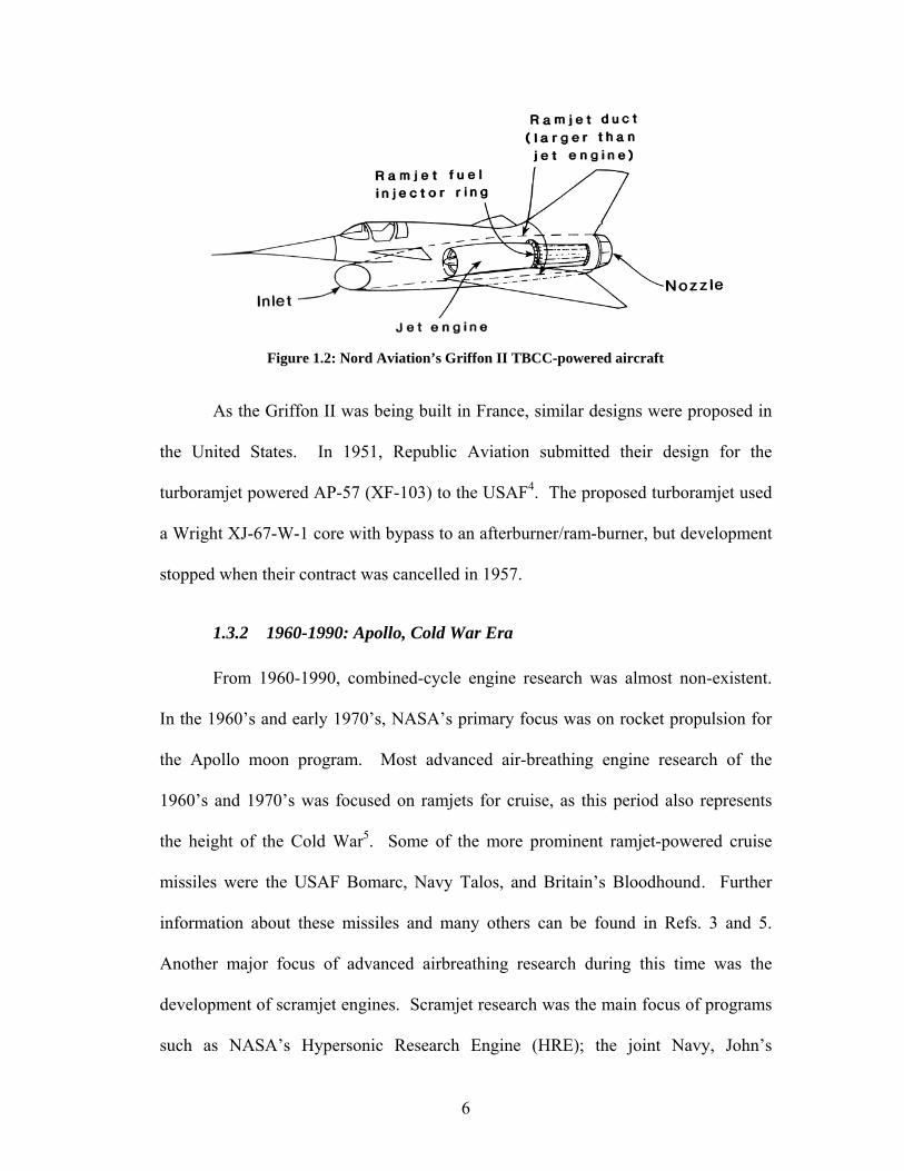
Figure 1.2: Nord Aviation’s Griffon II TBCC-powered aircraft
As the Griffon II was being built in France, similar designs were proposed in
the United States. In 1951, Republic Aviation submitted their design for the
turboramjet powered AP-57 (XF-103) to the USAF4. The proposed turboramjet used
a Wright XJ-67-W-1 core with bypass to an afterburner/ram-burner, but development
stopped when their contract was cancelled in 1957.
1.3.2 1960-1990: Apollo, Cold War Era
From 1960-1990, combined-cycle engine research was almost non-existent.
In the 1960’s and early 1970’s, NASA’s primary focus was on rocket propulsion for
the Apollo moon program. Most advanced air-breathing engine research of the
1960’s and 1970’s was focused on ramjets for cruise, as this period also represents
the height of the Cold War5. Some of the more prominent ramjet-powered cruise
missiles were the USAF Bomarc, Navy Talos, and Britain’s Bloodhound. Further
information about these missiles and many others can be found in Refs. 3 and 5.
Another major focus of advanced airbreathing research during this time was the
development of scramjet engines. Scramjet research was the main focus of programs
such as NASA’s Hypersonic Research Engine (HRE); the joint Navy, John’s
6

Hopkins/APL SCRAM program; and the National Aero-Space Plane program. There
were, however, a few notable programs from 1960-1990 which dealt primarily with
combined-cycle engines.
Zipkin and Nucci presented their analysis of several “Composite Airbreathing
Systems” at the 4th AGARD colloquium on “High Mach Number Airbreathing
Engines” in 1960. They performed a vehicle-level analysis to determine the impact
of air-breathing/rocket multistage vehicles for satellite launch and long-range cruise.
Their analysis was primarily system level, with very little information on the specifics
of the airbreathing engines, but they concluded that a horizontally launched air-
breathing first stage can provide twice the payload fraction of a traditional, vertically
launched rocket6.
From 1965-1967, under the NASA-sponsored Synerjet program, Marquardt,
Rocketdyne, and Lockheed jointly examined several combined-cycle engine and
vehicle concepts. This study was originally limited to integrating only ramjet and
rocket components, but found that the addition of a low-pressure ratio fan greatly
increased the payload capacity of their candidate vehicles. This program also
intended to focus on single-stage-to-orbit (SSTO) concepts, but actually found that
TSTO vehicles were the only technologically feasible option7.
One of the most successful TBCC examples from the United States is
Lockheed’s SR-71 program, which ran from the early 1960’s to 19898. The SR-71
was propelled by two Pratt & Whitney J58 “bleed bypass” engines, illustrated in Fig.
1.39.
7

Figure 1.3: Sketch of P&W J58 “bleed bypass” engine
These engines allowed the inlet air to bypass the combustor and turbine by bleeding
part of the flow off of the compressor and ducting it back into an afterburner/ram-
burner. Powered by the J58 engines, the SR-71 was able to take off and fly up to a
top speed of Mach 3+.
1.3.3 1990-Present: RLV Concepts for Access-to-Space
Over the past decade, combined-cycle engines have been reexamined for
space launch to respond to the demand for cheaper, safer launch vehicles to replace
the Space Shuttle. Bowcutt, Gonda, et al. and Hatakeyama, McIver, et al., compared
many RLV concepts on the basis of cost, performance, and operational parameters,
finding that airbreathing launch systems require almost twice the development costs
but half the operating costs of traditional launch systems10,11. For a launch program
longer than approximately 10 years, the TSTO airbreathing RLV system would be the
least expensive of all options.
8

Figure 1.4: SAIC’s ICM-3 RLV concept12
Figure 1.5: Boeing’s FASST concept
SAIC’s ICM-3 concept, Fig. 1.4, is a TSTO RLV utilizing RBCC 1st-stage propulsion
and pure rocket 2nd-stage. Escher and Christensen concluded that the optimal staging
Mach number for this system is Mach 7.212. As illustrated in Fig 1.5, Boeing’s
“Flexible Aerospace System Solution for Transformation” (FASST) concept is
similar to the ICM-3, except utilizing a turbojet-powered 1st-stage and RBCC-
powered 2nd-stage. The staging Mach number for the FASST vehicle was chosen to
be Mach 4, the limit of NASA’s Revolutionary Turbine Accelerator (RTA) 1st-stage
engine13. A final example of TSTO RLV comes from Mehta and Bowles at NASA
Ames, who found that a TBCC-powered 1st-stage and pure rocket-powered 2nd-stage,
separating at Mach 10, is the best option for reducing the cost and increasing the
safety and reliability of space launch14.
9

1.3.4 1990-Present: TBCC Engine Studies
Bossard and Thomas15,16 and Christensen17,18 have published several studies
specifically focused on the solid-fuel gas generator air turborocket. This engine is
primarily used in missile and rocket applications, but a similar form can be applied to
non-military systems. The details of liquid-fueled air turborocket operation will be
discussed in the following chapter. In 1997, Bossard and Thomas designed
turbomachinery specifically for the solid-fuel air turborocket. They concluded that
the fuel type and chemistry drives the turbomachinery design. The use of this
turbomachinery for missile propulsion provided three times the thrust of a
comparable turbojet and over twice the specific impulse of a comparable pure-rocket
system. In 1999, Christensen compared the solid-fuel air turborocket, turbojet, and
solid rocket motor on the basis of range and flight time for a missile system. He
concluded that, for a given range, the turborocket system reduced the turbojet flight
time by a factor of three. Similarly, for a given volume, the turborocket produced
double the flight time and range of a solid rocket. Bossard and Thomas studied the
influence of turbomachinery characteristics on turborocket performance in 2000.
They found that the turborocket is less sensitive to variations in compressor and
turbine efficiency, but more prone to problems with surge and stall. Finally, in 2001,
Christensen examined the accuracy of different engine chemistry models for the air
turborocket turbine. He found that the turbine flow is non-ideal and reacting. An
assumption otherwise would falsely predict two separate fuel ratios corresponding to
maximum specific impulse, when in reality there is only one.
10

NASA’s now-defunct Revolutionary Turbine Accelerator (RTA) program
represents the most recent work in TBCC development in the United States. The goal
of this program was to develop a turbine-based engine capable of flying at Mach 4+
with a minimum thrust-to-weight of 719. This program also planned to improve the
maintainability and operability of these engines, enabling the “airplane-like”
operation of the RLV concepts mentioned previously. The first stage of the RTA
program was the RTA-1 test bed, which was a “turbofan ramjet” based on an existing
General Electric YF120 core. More advanced engines and flight tests were planned,
but the program was cancelled in mid-2004.
1.3.5 1990-Present: TBCC Engine Comparisons
Several recent studies have compared specific TBCC engines on various
benchmarks. In 1990, Stricker and Essman used computational studies to compare
dry and afterburning turbojet, turboramjet, and air turborocket engines on the basis of
both installed and uninstalled engine performance for both cruise and acceleration.
They concluded that, although the air turborocket was able to produce greater thrust
at the same specific impulse, the afterburning turbojet was superior because it
provided competitive performance with much lower technological risk than the other
engines20. In 1995, under France’s PREPHA program, Lepelletier, Zendron, et al.
compared several RBCC and TBCC engines for SSTO launch systems. They found
that despite producing the highest specific impulse, a turbojet-based system was the
heaviest of all, to the point of infeasibility. The other concepts were to be studied
further; specifically considering an expander-cycle air turborocket in addition to the
gas generator air turborocket originally studied21. In 2001, Dupolev, Lanshin, et al.
11
compared many international RLV engine and vehicle designs from the past 15-20
years. The designs were compared on the basis of payload fraction and categorized
by separation Mach number. For near term technology (2005-2010), it was
concluded that a system with a separation Mach number of approximately 6, like
Russia’s MIGAKS concept, would be best. For more advanced technological
capabilities (2015-2020), the optimal staging Mach number would range between 8
and 10, with a scramjet mode added to the first stage propulsion system22.
Over the past few years, Japan’s ATREX program has also produced several
TBCC analysis projects similar to the one at hand. In 2001, Isomura and Omi,
Kobayashi, Sato, and Tanatsugu, and Kobayashi and Tanatsugu all presented their
findings from the comparison of TBCC engines for the 1st-stage of a TSTO RLV23-25.
Isomura and Omi compared a precooled turbojet and expander-cycle air turborocket
up to Mach 6, looking at trade studies on the variation of thrust and specific impulse
with fan and compressor pressure ratio, compressor efficiency, turbine inlet
temperature, and turbine efficiency. The trade studies showed that improvements in
turbine efficiency will do little to improve turborocket performance and that both
engines share similar technological limitations. Both engines were able to produce
similar thrust at transonic and high-speed conditions, but the turbojet was found to be
more efficient below Mach 3 while the turborocket was more efficient above Mach
323. Kobayashi, Sato, and Tanatsugu used genetic algorithm optimization to
determine the optimal propulsion system for the 1st-stage of a TSTO system, based on
minimum gross take-off weight (GTOW). Their baseline vehicle was a more
traditional cylindrical fuselage, delta-wing configuration with the candidate engines
12

(precooled turbojet, precooled expander-cycle turborocket, precooled gas generator
turborocket, and turboramjet) mounted on pylons beneath the wing. They concluded
that the turborocket cycles were limited by low turbine efficiency and the precooled
turbojet produced the lowest GTOW. The greatest limitation of the Turboramjet was
the requirement of a large ram-duct, which could be alleviated with more extensive
engine-airframe integration24. Kobayashi and Tanatsugu performed a similar
analysis, optimizing for maximum payload fraction in stead of minimum GTOW.
They concluded that the precooled turbojet was superior to the turborocket and
turboramjet cycles, but also examined the limitations of the turborocket cycles more
closely. The stored oxidizer required by the gas generator enhanced its ability to
maintain a high turbine inlet temperature, but incurred a specific impulse penalty that
made it the worst performing option of all. Both the gas generator and expander-cycle
turborockets were also limited by the turbine efficiency, but only the expander-cycle
would benefit from increased turbine inlet temperature25.
13

CHAPTER 2: ENGINE CYCLES
2.1 Brayton Cycle
The open Brayton cycle is the ideal thermodynamic cycle upon which all
modern aircraft engines are based. The term “open” refers to the fact that the engine
exhaust and inlet are not connected, leaving an open-loop with a constant influx of
fresh air. This is in contrast to, for example, the closed-loop refrigeration cycle,
where a fixed mass of refrigerant continually flows through the condenser,
evaporator, etc.
Figure 2.1: Pressure-volume and temperature-entropy
diagrams for the ideal Brayton cycle
The ideal Brayton cycle, as depicted by T-s and P-v diagrams in Fig 2.1,
consists of three basic processes: adiabatic compression (1-2), isobaric heat addition
(2-3), and adiabatic expansion (3-4). The term “open” refers to the fact that the cycle
loop is not actually closed from step (4) to step (1). For actual aircraft engines, these
processes are, of course, non-ideal and occur in separate engine components.
The thermal efficiency of a Brayton cycle engine can be expressed as a
function of the compression ratio from step (1) to (2), and the specific heat ratio of
the working fluid26.
14

γγ
η
1
1
2, 1
−−
⎟⎟⎠
⎞⎜⎜⎝
⎛−=
PP
Braytonth (2.1)
As illustrated by Eq. 2.1, the cycle efficiency of a Brayton engine can be maximized
by increasing the pressure as which heat is added. With this relation in mind, aircraft
engines will generally attempt to produce the highest pressure ratio possible, in order
to attain the highest possible cycle efficiency. As will be seen shortly, however, the
pressure ratio is generally limited by other engine constraints.
2.2 Ramjet
The ramjet is the simplest form of airbreathing engine. It uses the kinetic
energy of the aircraft alone to compress the freestream air, requiring no moving parts.
The compression process is performed using shockwaves and/or a diffuser section,
converting kinetic energy of the freestream air into internal energy in the form of
increased temperature and pressure. As such, ramjets are most effective at high
speeds, and cannot produce static thrust.
Figure 2.2: Ramjet flowpath
15

2.2.1 Flowpath
A typical ramjet flowpath is illustrated in Fig. 2.2. Freestream air (0) passes
through the inlet, from stations (1) to (5). Fuel is then mixed and combusted with the
inlet air from stations (5) to (6), further increasing its internal energy. After
combustion, the hot, high pressure products expand through a nozzle from (6) to (e),
converting the increased internal energy to excess kinetic energy. The increase in
kinetic energy of the air across the engine produces thrust, propelling the vehicle
forward.
2.2.2 Operation
For a given trajectory, ramjet performance is defined primarily by the inlet
geometry and combustor fuel flow-rate. For this project the inlet geometry is fixed,
so the only variable defining ramjet operation is the fuel-air equivalence ratio. The
equivalence ratio is defined as a “ratio of ratios” between the fuel-air ratio seen in the
combustor and the stoichiometric ratio for that fuel type.
.
.
stoich
burn
ff
≡Φ (2.2)
Theoretically, equivalence ratio can range from zero to infinity, where ratios above
1.0 are referred to as “fuel rich” because there will be excess fuel left over after
combustion. The use of equivalence ratio, in lieu of fuel-air ratio, in this project
allows a more direct comparison between operation with both hydrogen and
hydrocarbon fuels, as their stoichiometric fuel-air ratios differ significantly.
16

2.2.3 Constraints
At low speeds, RJ performance is limited by the inlet’s ability to provide
sufficient pressure ratio to the engine. As discussed for the general Brayton cycle, a
lower pressure ratio corresponds to lower cycle efficiency. In general, RJs are best
suited to supersonic flight, where the inlet can take advantage of high pressure ratios
across shockwaves in the inlet. As indicated in the previous work, subsonic RJ
operation is possible, but is more often limited to flight speeds above approximately
Mach 2.
At high speeds, RJ operation is limited by dissocciative and high temperature
effects in the combustor. This constraint is affected by a combination of flight speed
and equivalence ratio, generally limiting ramjet operation to approximately Mach 6.
At this speed, the temperature in the combustor is high enough that the water
produced by the combustion of hydrogen and oxygen will dissociate back into the
reactants. Additionally, the reactant molecules will dissociate into their atomic forms,
and the energy from combustion will remain stored in the exhaust gas, in stead of
being converted to thrust while expanding through the nozzle. Thus, this limit is
primarily chemical, not material, in nature.
RJitTT ,lim6 ≤ (2.3)
The temperature limit can be alleviated by reducing the strength of the
shockwaves in the inlet, thus maintaining supersonic flow throughout the combustor.
This type of engine is generally referred to as a “supersonic combustion ramjet,” or
“scramjet.” Scramjet operation is most effective above Mach 5, so it will not be
considered further for this project.
17

2.3 Turbojet
The turbojet engine can be defined as a ramjet that has been corrected for low-
speed flight. At low speeds, a diffuser alone cannot sufficiently provide the high
compression ratio that is required for efficient Brayton cycle operation. A turbojet
engine utilizes a mechanical compressor to increase the temperature and pressure of
the inlet air, providing a higher pressure ratio than could be delivered by the inlet
alone and increasing the overall cycle efficiency. The compressor is driven by a
turbine, which draws power from the expansion of combustion products. The use of
mechanical compression allows the turbojet to operate at static conditions, as
evidenced by most commercial and military aircraft flying today.
The temperature increase, and thus pressure ratio, cycle efficiency and
operation, of a TJ is primarily limited by the turbine inlet temperature. The heat
addition from the combustor must be limited so that the material limits of the turbine
are not exceeded. The turbine is made up of many fine blades that operate on the hot
gases immediately downstream of the combustor. As such, these blades are more
difficult to cool and are more sensitive to high temperature than the combustion
chamber itself. The turbine inlet temperature limit is defined by the turbine materials
and cooling and is generally lower than the combustion limit seen in a ramjet.
Afterburners are sometimes added to turbojets, injecting and combusting
additional fuel downstream of the turbine. This increases the temperature of the air
further and adds additional fuel mass to the flow, both of which increase the thrust of
an engine. Afterburners are most common in military aircraft, which can sometimes
afford sacrifices in fuel efficiency in exchange for additional thrust.
18

Figure 2.3: Turbojet flowpath
2.3.1 Flowpath
A turbojet flowpath, as shown in Fig. 2.3, begins in the same manner as the
ramjet. The freestream air (0) moves across the inlet, from stations (1) to (2),
undergoing some compression if the aircraft is in flight. The compressor acts in a
similar manner to the inlet, increasing the temperature and pressure of the air from
station (2) to (3). The main difference being that the compressor is mechanically
driven by the turbine, allowing it to increase the internal energy of the flow, even at
zero velocity. The compressed air then enters the combustor, which operates in the
same manner as the ramjet. The combustion products then expand through a turbine
from stations (4) to (5), whose sole purpose is to drive the compressor. The turbine
operates in reverse from the compressor, converting the energy of the combustion
products into shaft work. The afterburner acts in the same manner as a ramjet
combustor, from stations (5) to (6). Finally, as in the ramjet, thrust is provided by the
acceleration of the engine exhaust through a nozzle from stations (6) to (e).
19

2.3.2 Operation
As with the RJ, TJ operation is defined by the inlet geometry and fuel-air
equivalence ratio. However, the turbomachinery also introduces the compressor
pressure ratio as an additional design parameter. The pressure ratio is defined as the
fractional increase in total pressure across the compressor.
2
3
t
tc P
P≡π (2.4)
High compressor pressure ratios provide two benefits for TJ operation. By increasing
the combustor pressure, they help reduce dissocciative effects and allow for more
efficient combustion at higher temperatures. Additionally, high compression ratios
lead to higher engine pressure ratios, and, as shown in the Brayton cycle analysis,
higher cycle efficiency. High pressure ratios are generally desirable, but a single
compressor stage can only provide a finite pressure ratio, so higher pressure ratios
also require multiple compressor stages, and thus greater engine weight and
complexity. This factor is neglected in the current analysis but is nonetheless
important.
2.3.3 Constraints
The primary constraint on TJ operation, as mentioned before, is the maximum
turbine inlet temperature (T4) limit.
turbitTT ,lim4 ≤ (2.5)
For a given inlet and trajectory, T4 can only be decreased by reducing the compressor
pressure ratio or fuel-air equivalence ratio. At very high speeds, the material limit of
the compressor is also a factor. Turbines are generally actively cooled, but that is
20

more difficult for a compressor, so its temperature limit is generally lower than that of
the turbine. As the air temperature increases across the compressor, this limit is first
reached at the compressor exit.
compitTT ,lim3 ≤ (2.6)
As the engine analysis will be performed automatically, a negative turbine exit
temperature could, hypothetically, be calculated. This would be physically
impossible, and in fact, even a very low turbine exit temperature would be unrealistic.
Thus, the turbine exit temperature is constrained so that is must be greater than a
specified minimum.
turbTT min,5 ≥ (2.7)
This constraint is required because otherwise, the computer model could allow a
design that combines a high compressor pressure ratio with a low turbine inlet
temperature, forcing the turbine to expand to a negative temperature in order to
satisfy an energy balance with the compressor. This situation is, of course, physically
impossible and, in a real engine, the compressor pressure ratio would be relaxed in
order to relieve the requirements on the turbine. However, as that feedback is not
present in the engine models here (which will be discussed in detail in the following
chapter), a constraint on minimum temperature is required.
2.4 Turbine-Bypass Engine
The primary objective of any TBCC engine is to increase the upper speed
limit of a traditional turbojet by alleviating or eliminating the turbine inlet
temperature limit. The turbine-bypass engine (TBE) does this by bypassing the
21

combustor and turbine altogether at high speeds. The TBE is a form of afterburning
turbojet that combines the operation of TJ and RJ cycles. At high speeds, the
turbomachinery of the afterburning turbojet becomes less important, as the inlet alone
can provide the necessary compression. At this point, the flow through the
compressor is ducted around the combustor and turbine, directly into the afterburner.
The amount of bypass flow can vary, with increasing amounts causing the afterburner
to operate more like a RJ combustor. This operation could theoretically allow a
single engine to operate from take-off up to Mach 6, the theoretical limit of RJ
performance.
Figure 2.4: TBE flowpath
2.4.1 Flowpath
Figure 2.4 depicts a typical TBE flowpath. The inlet operates in the same
manner as in the ramjet and turbojet, compressing the freestream (0) from station (1)
up to the compressor face (2). The first compressor stage compresses the entire inlet
flow from location (2) to (8). At this point, bypass flow is bled off of the compressor
into the bypass duct. The non-bypass flow will then pass through a second
compressor stage, from location (8) to (3). The non-bypass, or “core,” section of the
22

TBE is simply a TJ engine, and may be treated as such. The non-bypass flow may be
treated as compressing in a single step, from (2) to (3). The combustor and turbine of
the TBE also act in an identical manner to the TJ. The bypass flow will pass through
a duct from (8) to (9), undergoing an area change in order to better condition the flow
for the afterburner. The turbine and bypass exit flows then mix and enter the
afterburner at station (5). The afterburner, from (5) to (6), and nozzle, stations (6) to
(e), act in exactly the same manner as the RJ burner and nozzle.
2.4.2 Operation
In addition to the traditional TJ parameters, TBE operation is also
characterized by the bypass and compressor staging ratios. The bypass ratio for the
TBE is defined as the ratio of bypass mass-flow to inlet mass-flow:
0mm
α bypassTBE &
&≡ (2.8)
At a bypass ratio of 0, all air will pass through the core and the engine will perform
like a pure turbojet engine. At a bypass ratio of 1, all inlet air will move directly to
the afterburner and the engine will behave like a ramjet. Intermediate bypass ratios,
however, provide the most interest as they combine the operation of both engines,
possibly providing performance superior to either engine alone.
The TBE uses a two-stage compressor, where the first stage acts on the entire
inlet flow and the second stage acts only on the core flow. The first stage is often
referred to as a “fan” because it generally operates with a low pressure ratio and high
flow-rate. The distribution between the two compressor stages is characterized by the
23

compressor staging ratio (βc). The compressor staging ratio is defined as the fraction
of compression occurring in the first stage:
totalc
stgcc
,
1.,
ππ
β ≡ (2.9)
Variations in compressor staging affect only the bypass flow. At a staging ratio of 0,
all compression occurs in the second stage and the bypass flow enters the
afterburning without undergoing any mechanical compression. This configuration is
sometimes referred to as “turboramjet”, where a turbojet core is essentially propelling
an attached ramjet. This is also the only form of TBE that allows full ramjet
operation (α=1), as some non-bypass flow would be required to operate the fan stage
for other configurations. At a staging ratio of 1, all compression occurs in the first
stage and the inlet flow is compressed entirely before bypass. Assuming a given
bypass ratio, the flow into the combustor will always undergo the same total
compression for any staging ratio.
2.4.3 Constraints
In addition the constraints of the previous engines, the bypass duct introduces
constraints that are specific to the TBE. For reasonable engine packaging, the area
change in the duct must be lower than a factor of 100 – representing no more than an
order of magnitude change in diameter for an axisymmetric duct. Additionally, to
prevent backflow in the bypass duct, the ratio of turbine exhaust pressure to duct
exhaust pressure is constrained to be less than 10. As this engine employs a ram-
burner (not scram-burner), the bypass velocity is constrained to be subsonic at the
duct exit. Finally, the afterburner fuel is assumed to react with only the fresh bypass
24

air, which translates to the afterburner equivalence ratio being less than or equal to
the bypass ratio.
10001.09
8 ≤≤AA
(2.10)
109
5 ≤PP
(2.11)
0.19 ≤M (2.12)
α≤Φ AB (2.13)
2.5 Air Turborocket
While the TBE alleviates the turbine inlet temperature limit of a traditional
turbojet by utilizing bypass flow at high speeds, the air turborocket (ATR) eliminates
this limit altogether by isolating the turbine from the inlet and compressor flow and
supplying it with stored, hot, high pressure gas. The hot gas alone passes through the
turbine, which still drives the compressor, drawing inlet air into the combustor, where
it reacts with the excess fuel in the hot gas leaving the turbine. The use of this stored
gas also requires operation with much lower turbine and compressor pressure ratios,
reducing the number of turbomachinery stages, and thus engine weight. This leads to
a greater sensitivity to turbine efficiency in the ATR as the turbine working fluid is no
longer air. The ATR also addresses the problem of low thrust of the TBE by
combining elements of turbojet and rocket engines to produce an engine with higher
thrust-to-weight across a wider range of Mach numbers than a traditional turbojet
engine, with higher specific impulse than a traditional rocket.
25

The ATR comes in two main forms, characterized by the source of the hot
gas. In a “gas generator ATR” (GG-ATR), the source of this gas is the combustion of
stored fuel and oxidizer in a gas generator. An “expander-cycle ATR” (EX-ATR), on
the other hand, utilizes pre-heated fuel alone, likely from engine cooling. This system
ultimately serves to decouple the turbine inlet temperature from the flight speed,
allowing the engine to operate across a larger range of Mach numbers than a
traditional turbojet.
Figure 2.5: GG-ATR (bottom) and EX-ATR (top) flowpaths
2.5.1 Gas Generator ATR Flowpath
The GG-ATR, shown in the bottom half of Fig. 2.5, provides hot gas to the
turbine from a gas generator, at station (4). The gas generator is essentially a rocket
chamber immediately upstream of the turbine and is supplied only with stored fuel
and oxidizer, at an extremely fuel-rich mixture. Only the gas generator combustion
products and excess fuel expand through the turbine, from (4) to (5), providing the
necessary shaft work to the compressor. The inlet and compressor operate in the
same manner as the turbojet, with a single compressor stage moving inlet air into the
26
combustor, from stations (2) to (3). For the ATR, however, the inlet air flows directly
to the afterburner, (5) to (6), where it mixes and burns with the excess fuel leaving the
turbine. The afterburner does not have its own fuel injectors. The afterburner and
nozzle are again identical to those of the TBE, TJ, and RJ.
2.5.2 Expander-Cycle ATR Flowpath
The greatest limitation of the GG-ATR is the use of stored oxidizer, which
greatly decreases specific impulse and creates a very high temperature flame in the
gas generator. The EX-ATR eliminates these issues by using the expansion of
pressurized, pre-heated, but un-combusted fuel to drive the turbine. This removes the
need for oxidizer altogether, as combustion only occurs with inlet air in the
afterburner. As illustrated in the top half of Fig. 2.5, the EX-ATR is almost identical
to the GG-ATR, simply lacking the stored oxidizer and combustion chamber
upstream of the turbine. The EX-ATR assumes that the fuel will be used for active
cooling, and then pumped into a chamber upstream of the turbine (4) at a high
temperature and pressure. The turbine is then powered, as in the GG-ATR, by the
expansion of the hot gas. From that point onward, the two ATR cycles are identical
in configuration and operation.
2.5.3 Operation
Regardless of gas source, ATR cycle performance is characterized by its
bypass ratio, which is defined as the ratio of mass-flow through the inlet to mass-flow
through the turbine:
27

turbine
inletATR m
mα&
&≡ (2.14)
Theoretically, the bypass ratio can range anywhere from zero to infinity. At very low
bypass ratio values, the majority of the engine mass flow comes from the stored
gases, and the ATR will behave like a rocket. Similarly, at higher bypass ratio
values, the gas generator or expander will simply act as a fuel injector and the engine
will behave similar to a turbojet. This illustrates another major benefit of the ATR
over other engines: it can provide higher thrust than a tradition turbojet engine when
needed, and then scale back to more efficient operation by simply changing the
propellant flow-rates in the engine. It should be noted that the higher thrust modes of
the GG-ATR will also give lower specific impulse than a traditional turbojet, as
stored oxidizer is being used.
As with any turbine-based engine, a compressor pressure ratio and fuel flow
rate are also required to fully define the cycle performance. For GG-ATR operation,
a fuel-oxidizer equivalence ratio must be specified for the gas generator. This term is
defined in the same manner as Eq. 2.2, but with fuel-oxidizer ratios in place of fuel-
air.
.,2
,2
stoichO
ggO
ff
≡Φ (2.15)
As the only substance passing through the turbine of an EX-ATR is fuel, its fuel-air
ratio is simply the inverse of the bypass ratio. Thus, only the bypass ratio and
compression ratio are required to fully define the EX-ATR.
28
2.5.4 Constraints
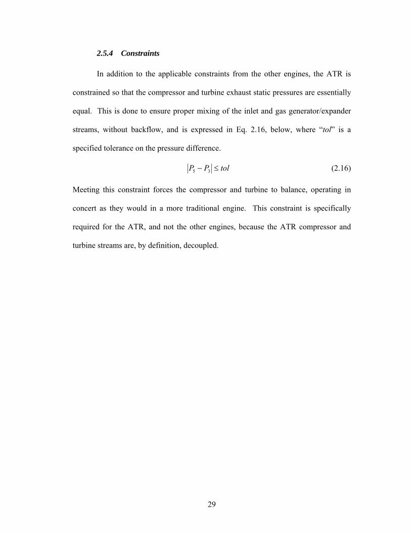
In addition to the applicable constraints from the other engines, the ATR is
constrained so that the compressor and turbine exhaust static pressures are essentially
equal. This is done to ensure proper mixing of the inlet and gas generator/expander
streams, without backflow, and is expressed in Eq. 2.16, below, where “tol” is a
specified tolerance on the pressure difference.
tolPP ≤− 35 (2.16)
Meeting this constraint forces the compressor and turbine to balance, operating in
concert as they would in a more traditional engine. This constraint is specifically
required for the ATR, and not the other engines, because the ATR compressor and
turbine streams are, by definition, decoupled.
29

CHAPTER 3: ENGINE ANALYSIS
3.1 General Analysis
Although they have different names, the aforementioned engines are all just
variations on the basic afterburning turbojet engine. As such, on a system level, the
analysis of each is identical. The thrust analysis presented here will begin at this
level, showing the basic equations of motion that are common to all airbreathing
engines. Subsequent sections will then address a component level analysis, which
will vary from engine to engine.
TBCC engine performance is quantified by the thrust and specific impulse.
This analysis begins with the familiar thrust equation27:
( ) eaeee APPumum=T −−− 00&& (3.1)
Equation 3.1 is simplified by assuming an ideal nozzle, where the exhaust expands
isentropically to atmospheric pressure, and by defining ℜ as the relative amount of
mass added to the inlet flow while passing through the engine. This parameter
accounts for all injected propellants and has distinct, engine-specific forms, as given
by Eq. 3.3.
( ) 000 1 umum=T e && −ℜ+ (3.2)
( )⎪⎩
⎪⎨
⎧
+−≡ℜ− ATR
TBEffTJRJf
abb
b
1
1,
ααα (3.3)
Thrust is then divided by the inlet mass flow-rate and local speed of sound. The
resulting term is referred to as “normalized thrust” and is a dimensionless quantity
30

that is independent of engine size and vehicle trajectory, allowing for direct
comparison between engines in a variety of applications.
( ) 00
1 Mau
+=am
T
a
e
a
−ℜ&
(3.4)
The velocity ratio in Eq. 3.4 can be further dissected using the definition of Mach
number:
aa
eee
a
e
RTγRTγM
=au (3.5)
By canceling the ideal gas constant from the numerator and denominator and
rewriting the exit temperature in terms of total temperature and Mach number, Eq. 3.5
becomes:
⎟⎠⎞
⎜⎝⎛ −
2211
e6
aa
teee
a
e
Mγ+Tγ
TγM=au (3.6)
A final expression for normalized thrust is derived by inserting Eq. 3.6 into Eq. 3.4
and using the assumption of isentropic expansion to replace Tte with Tt6.
( ) 0
2
6
0
211
1 MMγ+Tγ
TγM+=am
T
e6
aa
t6e
a
−⎟⎠⎞
⎜⎝⎛ −
ℜ&
(3.7)
Specific impulse is found by multiplying the normalized thrust by the local
speed of sound and dividing by the weight flow rate of fuel (or fuel plus oxidizer for
rocket systems).
ℜ⎟⎟⎠
⎞⎜⎜⎝
⎛ga
amT=
mgT=I a
aox+fuelsp
0. && (3.8)
31

The exit Mach number, required in order to calculate normalized thrust, is derived
from the traditional isentropic pressure relation at the nozzle exit plane:
126 6
6
21
1−
⎟⎠⎞
⎜⎝⎛ − γ
γ
ee
te Mγ
+=PP (3.9)
An expression for exit Mach number is found by solving Eq. 3.9 for an ideal nozzle,
where Pe=Pa and Pte=Pt6.
⎟⎟⎟
⎠
⎞
⎜⎜⎜
⎝
⎛−⎟⎟
⎠
⎞⎜⎜⎝
⎛−
−
11
2 6
6 1
6
γγ
a
t6e P
Pγ
=M (3.10)
The atmospheric and freestream properties required for Eqs. 3.7-3.10 are
given by the trajectory, which will be discussed shortly. The afterburner exit
properties, denoted by subscript “6,” required in Eqs. 3.7 and 3.10 are found by
calculating the temperature, pressure, and Mach number between engine components,
starting from the inlet and working downstream. With these component properties,
which are the topic of the following section, the values for normalized thrust and
specific impulse can be calculated.
3.2 Component Analysis
3.2.1 Inlet
The inlet, as shown in Fig. 3.1, is chosen to be a three-shock inlet, consisting
of two oblique shocks and a terminating normal shock. When the upstream Mach
number normal to a given shock is subsonic, that portion of the inlet is assumed to
have no effect on the flow.
32

Figure 3.1: Inlet diagram
Each portion of the inlet is treated as a two-dimensional wedge, with a given half-
angle (θ). For the two oblique shocks, the shock angle (β) is found using the tradition
θ-β-M relation:
( ) ( ) ( )( ) ( ) ( )θθMγ
βMγ+=θβcossin1
sin12tan 211
2211
−−
− (3.11)
Once the shock angle has been calculated, the normal component of the Mach number
can be calculated, and the properties behind the oblique shock can be found in the
same manner as a normal shock27,28:
( )βsin11 MM n = (3.12)
11
21
2
21
1
1
1
21
22
−−
−+
=
n
n
n
M
MM
γγ
γ (3.13)
⎟⎟⎠
⎞⎜⎜⎝
⎛++
= 221
211
12 11
n
n
MM
PPγγ (3.14)
2
1
2
2
1
212 ⎟⎟
⎠
⎞⎜⎜⎝
⎛⎟⎟⎠
⎞⎜⎜⎝
⎛=
n
n
MM
PPTT (3.15)
( )θβ −=
sin2
2nM
M (3.16)
Equations 3.12-3.16 are used to find the properties behind the two oblique inlet
shockwaves. By definition, the flow upstream of the normal shock is perpendicular
to the shock, so Eqs. 3.12 and 3.16 are omitted for that shock.
33

3.2.2 Fan/Compressor
For the TBE, the pressure rise across the first compressor stage is given by the
total compression ratio and the compressor staging ratio. The temperature rise across
the compressor is based on an isentropic relation, accounting for compressor
efficiency29.
cct2t8 βπP=P (3.17)
( )⎥⎥
⎦
⎤
⎢⎢
⎣
⎡+
−=
−
112
2 1
28c
cctt TT
ηβπ γ
γ
(3.18)
For existing engines, this efficiency is generally known, or at last calculable, but the
efficiency in the TBCC engines of this study is unknown. Thus, this value will be
treated as an assumed input parameter, and will be the subject of subsequent trade
studies. Properties behind the second TBE compressor stage, or behind the entire
compressor for the other engines, are found in the same manner as above, with a
similarly assumed efficiency.
ctt PP π23 = (3.19)
( )⎥⎥
⎦
⎤
⎢⎢
⎣
⎡+
−=
−
112
2 1
23c
ctt TT
ηπ γ
γ
(3.20)
3.2.3 Turbine
The temperature change across the turbine is specified by an energy balance
between the compressor and turbine.
tcpccttptt TCm=TCm ∆∆ && (3.21)
Assuming a single turbine stage, Eq. 3.21 can be re-written as follows:
34

tct
c
pt
pct4t5 T
mm
CC
T=T ∆−&
& (3.22)
Or, for N compressor stages:
∑ ⎟⎟⎠
⎞⎜⎜⎝
⎛∆−
N
iti
t
i
pt
pct4t5 T
mm
CC
T=T&
& (3.23)
From Eq. 3.23, each engine has a unique expression for turbine exhaust temperature,
as given below:
( ) ( )
( )⎪⎪⎪⎪⎪
⎩
⎪⎪⎪⎪⎪
⎨
⎧
−−
⎟⎠⎞
⎜⎝⎛
−−
+−+
−
⎟⎟⎠
⎞⎜⎜⎝
⎛+−
−
ATRTTC
CT
TBETT
TTfC
CT
TJfTT
CC
T
=T
ttpt
pct4
tttt
bpt
pct4
b
tt
pt
pct4
t5
23
2883
23
11
1
α
α (3.24)
As in the compressor, an expression for turbine pressure change in terms of
temperature change is based on an isentropic relation, accounting for turbine
efficiency.
1
4
545
4
4
111−
⎥⎥⎦
⎤
⎢⎢⎣
⎡⎟⎟⎠
⎞⎜⎜⎝
⎛−−=
γγ
η t
t
ttt T
TPP (3.25)
Once again, the exact value of this efficiency is unknown for the TBCCs of this
study, and will be an assumed parameter and the subject of subsequent trade studies.
3.2.4 TBE Bypass Duct
Assuming uniform density and pressure across the compressor face and unit
inlet cross-sectional area, the area of the bypass and core are directly related to the
bypass ratio:
35

α=8A (3.26)
α−=13A (3.27)
The bypass area change is designed such that the duct exhaust velocity will be equal
to the turbine exhaust velocity, providing optimal engine efficiency. This design is
analogous to the same principle used in the design of a traditional turbofan engine. It
should be noted that although the exit velocity of the turbine and duct will be equal,
the Mach numbers of each will generally be quite different, as the temperatures, and
thus sonic velocities, of the streams will differ.
The optimal duct exit area and exit properties will be found by assuming an
isentropic area change. The first step in this process is to find the critical
(corresponding to M=1) properties, for use as a reference point.
⎟⎠⎞
⎜⎝⎛ −+
+≡ 2
88
8 211
12 MC γ
γ (3.28)
( )121
88* 8
8
−+
−
= γγ
CMAA (3.29)
CTT 8* = (3.30)
18
* 8
8
−= γγ
CPP (3.31)
*8
* RTa γ= (3.32)
The desired condition for the bypass exit is equal velocity to the turbine exit:
5559 RTMu γ= (3.33)
The bypass exit conditions can be found by inserting the desired condition from Eq.
3.33 into the isentropic flow relations, reversing the process of Eqs.3.28-3.32.
36

21
82
*98
9 21
21
−−
⎥⎥⎦
⎤
⎢⎢⎣
⎡ −−⎟
⎠⎞
⎜⎝⎛+
=γγ
auM (3.34)
⎟⎠⎞
⎜⎝⎛ −+
+≡ 2
98
8 211
12 MC γ
γ (3.35)
( )121
19
*9
8
8
−+
−= γγ
CMAA (3.36)
1*9
8
8
−−
= γγ
CPP (3.37)
1*9
−= CTT (3.38)
3.2.5 Burner/Afterburner/Gas Generator
The mixing and combustion for the burner, afterburner, and gas generator is
handled entirely by NASA’s Chemical Equilibrium with Applications (CEA) code30.
This code calculates the equilibrium chemical and thermodynamic properties of a
mixture of gases based on the minimization of Gibb’s free energy. This code is
required to determine the thermodynamic properties at the turbine and nozzle inlet,
where the presence of fuel and high-temperature combustion products precludes the
usual assumption of a specific heat model based on air alone. This is especially
important in the turbine analysis for the ATR cycles, where the turbine working fluid
is comprised entirely of excess fuel and/or combustion products. Specific details
about the analysis behind CEA and its implementation can be found in Ref. 30.
Reference 31 gives full details about the input, output, and usage of CEA, but those
specifically pertaining to this project are given below.
The combustor, gas generator, and afterburner are all modeled as infinite-area-
combustor rockets in CEA. For input, CEA requires the mass-fraction and
37

temperature of each reactant, along with a chamber pressure. CEA returns many
equilibrium chemical and thermodynamic properties, but the ones of interest for the
engine models are: temperature, pressure, constant-pressure specific heat, and specific
heat ratio. These properties are calculated at a theoretical throat, as the turbine will
have choked flow to prevent backflow, and the afterburner exhausts directly to a
supersonic nozzle. CEA also returns a list of all exhaust products and their relative
mass fractions.
The fuel inlet temperature and ATR chamber pressures are assumed values,
while the burner and afterburner pressure and air temperature are based on the
compressor and turbine exit properties. The TBE afterburner reactants account for
the bypass air, afterburner fuel, and the turbine exhaust products. Similarly, the ATR
afterburner models include all turbine exhaust products and the inlet air as reactants.
This allows for an accurate model of the excess-fuel combustion of the GG-ATR.
3.2.6 Expander
The expander section of the EX-ATR consists of non-reacting flow, but CEA
is also employed to calculate the appropriate thermodynamic properties. This process
is required because the turbine working fluid in the EX-ATR is pure fuel, so the
constant-pressure specific heat and specific heat ratio are unknown. These properties
are found by performing an assigned-temperature/pressure problem in CEA. This
calculation requires only the fuel temperature and pressure and returns the same
equilibrium thermodynamic properties as the combustion model above.
38

3.3 Assumptions
Several assumptions have been made to simplify the engine analysis. The
ratio of specific heats is assumed constant for each engine component, but allowed to
vary between components. As mentioned previously, the specific heat and specific
heat ratio of the turbine and nozzle are calculated directly in CEA. For components
acting on air alone, Eq. 3.39 gives the specific heat ratio of air as a function of static
temperature, and is based on a curve-fit of available data.
( )⎪⎩
⎪⎨⎧
∗−
≤=
K>TT
KT
600ln0.08381.936
6001.4γ (3.39)
The trajectory for every engine assumes an approximately constant dynamic
pressure of about 1 atm., with an acceleration/climb phase up to Mach 2. As
mentioned previously, the inlet is chosen to be a three-shock inlet, consisting of an
oblique shock, turning shock, and terminating normal shock. When the Mach number
normal to any one of these shocks is less than 1.0, that portion of the inlet is assumed
to have no effect on the flow. The compressor and turbine are assumed to operate as
disc actuators with user-specified efficiencies. The turbine is always assumed to have
a moderate exit Mach number of about 0.5, to maintain a high engine exit Mach
number. For the TJ and TBE, the compressor exit Mach number should be low for
efficient combustion, and is assumed to be 0.05. For the ATR cycles, however, the
compressor exhausts to the afterburner so a moderate exit Mach number of 0.5 is
assumed, similar to the turbine.
39

Combustion is permitted with either hydrogen or hydrocarbon fuel. For
hydrocarbon combustion, gaseous Jet-A is the assumed fuel. Table 3.1 gives the
stoichiometric fuel-air and fuel-oxygen ratios assumed for each fuel.
Table 3.1: Assumed stoichiometric fuel ratios
Fuel Type Stoich. Fuel-Air Ratio
Stoich. Fuel-O2 Ratio
H2 0.0289 0.125
Jet-A 0.0678 0.293
For the TJ, RJ, and TBE burners, GG-ATR gas generator, and TBE afterburner, a fuel
inlet temperature of 200 K is assumed. The ATR afterburners calculate the fuel
temperature directly from the turbine exhaust. The GG-ATR gas generator pressure
is assumed to be 4000 kPa (about 40 atm.). This is comparable to the gas generator
pressure in the Atlas rocket32. As it has no combustor upstream of the turbine, the
EX-ATR assumes the fuel has been used for active cooling, with an inlet temperature
on the order of 1000 K, and a pressure of 2000 kPa. With the exception of the GG-
ATR chamber pressure, the aforementioned values have been chosen as educated, but
somewhat arbitrary estimations, and will be the subject of trade studies in Chap. 5.
40

CHAPTER 4: ENGINE OPTIMIZATION
4.1 Program Structure
The TBCC engine analysis and optimization is performed using a custom
computer code written in a combination of FORTRAN, C, and C++. All new code
for this project, which includes the driver routine, engine models, and subroutine
interfaces, is written in C++. The code also utilizes CEA and pre-existing
optimization subroutines, which are written in FORTRAN 77 and C. The code
performs a quasi one-dimensional thermodynamic cycle analysis, calculating the
pressure, temperature, and Mach number at each position in the flowpath in order to
calculate normalized thrust and specific impulse, as given by Eqs. 3.7 and 3.8,
respectively. This process is repeated for a user-defined range in Mach number, such
that the output consists of a list of optimum values of normalized thrust, specific
impulse, and the design variables, corresponding to each value of Mach number.
The code is modular, with separate driver, optimization, and analysis routines
linked as shown in Fig. 4.1. The driver routine reads the main input file, in which the
user specifies the engine cycle, fuel type, optimization method, Mach number range
and discretization, and limits on each design variable. The driver repeats the
optimization process across the user-specific range of Mach numbers, calling the
appropriate optimizer, reading the optimization results, and writing them to the output
file. The optimization routines communicate with each engine module separately,
which, in turn, communicates directly with CEA, as needed.
41

TBCC TBCC Driver Input Output Routine
Figure 4.1: TBCC program flowchart
4.2 Optimization
The engine analysis is approached as an optimization problem, where the
bypass ratio, compressor pressure ratio, and fuel flow rates are treated as design
variables, optimized in order to maximize a given objective function at each value of
Mach number, while also satisfying the constraints given in Chap.2. As such, the
model produces the best possible engine performance for the given flight Mach
number and component limits.
The driver program allows the user to specify one of three optimization
schemes: gradient-based, probabilistic, or a hybrid optimizer that combines the two.
The hybrid scheme is used exclusively in this project, as it combines the strengths and
combats the weaknesses of its component methods. The other methods may still be
CEA
Optimizer
DOT GA
Loop for Mmin<M<Mmax
GA Input
RJ TJ TBE GGATR EXATR
42

used separately, however, either for debugging purposes, or when analyzing a simpler
system that can be solved by gradient-based optimization alone.
4.2.1 Gradient-Based Optimization
Gradient-based, or “hill-climbing,” optimizers, as indicted by their name, use
information about the rate-of-change of an objective function in order to follow a path
to the optimum value for that function. In order to follow this path, an initial, feasible
design must be specified as a starting point for the optimization, and the gradient of
the objective function must be calculable. The greatest benefit of gradient-based
methods is computational efficiency. These methods were developed before the time
of computers, and are founded on basic mathematical analysis, making them very
fast. Their greatest limitations, however, are that they require a continuous design
space and cannot guarantee convergence to a global optimum when multiple local
optima are present. Unfortunately, that type of design space is common in engine
analysis, where different combinations of compression and fuel ratio can result in
many local optima.
One example of a very simple gradient-based method is “steepest ascent.” In
this method, the optimizer determines the gradient of the objective function at the
initial design, and then travels in the direction that provides the greatest increase in
that function. The optimizer stops at the maximum point in that direction and
calculates the gradient again. The gradient may be calculated either analytically or
numerically, and the process is repeated until the optimizer reaches a local maximum,
in which case the gradient would be zero. Figure 4.2, from VMA Engineering’s DOT
User Manual33, illustrates the principle behind “hill-climbing” methods pictorially.
43

Figure 4.2: A comic representation of “hill-climbing” optimization
There exist, of course, more sophisticated gradient-based methods which can
handle more complex design spaces and constraints; for more specific information
about those methods, see Ref. 34. The gradient-based method of choice for this
project is the Modified Method of Feasible Directions (MMFD), in VMA
Engineering’s Design and Optimization Tools (DOT) code. DOT is a commercially
available, gradient-based optimization package which provides several unconstrained
and constrained optimization methods. MMFD was chosen for this project as it is
DOT’s default constrained optimizer and is sufficiently reliable, efficient and robust.
A full explanation of MMFD can be found in the DOT Manual.
DOT is linked directly to the engine optimization code as a FORTRAN
subroutine, and allows for the customization of dozens of parameters through input
arrays. With the exception of the values listed in
Table 4.1, below, the default values for these parameters have proven sufficient.
Table 4.1: DOT non-default input parameters Parameter Definition Default
Value Assigned
Value ct Active constraint tolerance -0.03 -0.01 ctmin Violated constraint tolerance 0.003 0.001
dabobj Maximum change in objective to indicate convergence 0.0001*ABS(F0) 0.0001
itrmop Number of consecutive iterations required to meet convergence criteria 2 10
44

The term F0, in the default value for DABOBJ, is the value of the objective function
at the initial design. Specific impulse has been chosen as the objective function, for
reasons to be explained in Section 4.2.4, and will generally be on the order of 1000
sec., so the assigned value for DABOBJ represents finer and more rigorous
convergence. The exact values for the assigned parameters have been determined on a
trial-and-error basis, chosen because they ultimately provide a better solution than the
defaults. The goal behind changing these parameters is to refine the optimization in
DOT, so that it can find the optimum more consistently and accurately, despite the
many constraints and sometimes convoluted design space of the more advanced
engine cycles.
Finer tolerances for both active (CT) and violated (CTMIN) constraints are
chosen in order to converge to an optimum with constraint values as close to critical
as possible. This is best understood by looking at the graphical representation of a
hypothetical constraint in Fig. 4.3.
Figure 4.3: Graphical representation of constraint tolerance,
courtesy of the DOT User Manual
45

The optimizer approaches the constraint from the feasible region, shown to the upper-
right of the constraint. In theory, a constraint becomes active when it is equal to zero.
However, in systems with multiple, intersecting constraints, it can be very
computationally inefficient for the optimizer to wait for the solution to exactly reach a
point where all constraints are critical. To remedy this, a constraint tolerance (CT) is
added, such that the constraint is considered active once its value is greater than that
of the tolerance, which is always a small negative value. Similarly, a constraint is
theoretically considered violated when it is greater than exactly zero. The addition of
a tolerance on violated constraints (CTMIN) performs a similar function by allowing
a constraint to be considered active until its value is greater than the tolerance. The
net result of the tolerances is to create a “cushion” at the constraints that allows the
solution to converge more quickly by counting the constraints as active even if their
values are not exactly equal to zero.
One drawback of using constraint tolerances, however, is that they can result
in less precise values for the optimum, as the solution converges before reaching the
theoretical optimum of the design space. The new values for CT and CTMIN have
been chosen because they still provide the benefits of using constraint tolerance, but
also increase the precision of the solution, in exchange for slightly less efficient
operation.
Non-default values for DABOBJ and ITRMOP are chosen to refine the
convergence as well. By forcing the optimizer to converge on a smaller criterion over
a longer number of iterations, the new input values tend to provide a more accurate
final solution. In general, with the default values for these parameters, DOT returns
46

an optimum very quickly, but even across a small design space, this value is not
always the global optimum. Refining the convergence criteria gives DOT the ability
to get past some of the complexities of the TBCC design space and be more likely to
locate the global optimum within a small region.
4.2.2 Probabilistic Optimization
While gradient-based methods are purely analytical, probabilistic methods are
purely computational in nature. These methods do not require an analytical
expression for the objective function, an initial design, or any gradients at all. All that
is required is a value of the objective function at any given point across the design
space. In probabilistic methods, the constraints are generally lumped into the
objective function, such that a combination of variables producing an infeasible
design returns a poor objective value. Probabilistic methods are generally iterative in
nature, where each subsequent iteration provides a design that is statistically closer to
the global optimum than the previous.
An example of a simple probabilistic method is “random choice.” In this
method, a certain number of random points in the design space are selected and
analyzed. The design point with the highest objective becomes the new optimum.
With an infinite number of points, random choice will actually scan the entire design
space, calculating the objective function for every possible combination of variables,
guaranteeing that the global optimum will be found. This, of course, would also
require infinite computational power.
More sophisticated methods use the same principles as random choice, but
modify the execution in order to locate the optimum in a more efficient manner than
47

just scanning blindly. The probabilistic optimizer chosen for this research is Genetic
algorithm (GA), as written by Ryan Starkey35. This optimizer was chosen for its ease
of integration into the entire engine package, and its validated usage at the University
of Maryland. The greatest benefit of GA is that it requires no knowledge of the
design space itself, and is not sensitive to multiple local optima, discontinuities in the
design space, or irregular objective functions or constraints. As it is based entirely on
the comparison between objective values of several designs, and not on the shape of
the design space itself, it is guaranteed to find the global optimum, assuming
sufficient convergence. The greatest weakness of GA, however, is that it is extremely
expensive and locally inefficient.
GA was originally developed by John Holland, with the goal of integrating the
processes of evolutionary biology into a problem-solving scheme36,37. GA is based
on the concept of survival-of-the-fittest, where the strongest designs (referred to as
“chromosomes”) reproduce most frequently, and their lineage evolves over many
generations into the optimum design. Processes such as reproduction, competition,
and mutation all take place, as in nature, so that, after many generations, the fittest
chromosomes converge to the global optimum. Each chromosome is a binary string
which represents a single design point in the system. Values for every design
variable can be decoded from that string in order to calculate a value for the objective
function. The GA process consists of four primary steps:
1. Initialize population at random
2. Evaluate each chromosome in population
3. Fittest members of population reproduce, with random mutation
48

4. Part of population is replaced by new chromosomes, creating new generation
Steps 2-4 are repeated until either: a) the solution converges such that a single
chromosome is the fittest for many consecutive generations, or b) a maximum
number of generations are reached without convergence. The exact values for these
generations are user-specified. For convergence to even be possible, the generation
number in b) must be greater than that in a); to guarantee convergence, though, the
value in b) should be as large as possible.
The GA optimizer allows many input parameters to specify details of the
optimization process, however, the only parameters varied from their default values
are those defining the population, convergence, and probability of mutation or cross-
over. Table 4.2 defines each of these parameters, and the non-default values selected.
Table 4.2: GA non-default input parameters Parameter Definition Value
ipop_length Population size 50
imax_gen Maximum number of generations 800
iconverge Convergence criteria 1 (objective function)
isteady Generations to converge 200
change Maximum change for convergence 0.1%
prob_ops Probability of cross-over or mutation operators being used 100%
A population size of 50 is selected to provide a good combination of precision and
efficiency for the optimizer. The GA solution converges once the objective function
maintains 200 consecutive generations with values less than 0.1% greater than the
current optimum. If the objective function of a particular chromosome exceeds this
limit, it becomes the new optimum, and the count for convergence restarts. If the
solution has not converged within 800 iterations, however, optimization ends, with
the current optimum value assumed to be the global optimum. A 100% mutation rate
49

enables faster convergence to the global optimum by allowing the optimizer to probe
regions of the design space that may not be found by reproduction alone. As with the
non-default parameters in DOT, the GA input values are determined through trial-
and-error; selected in order to provide a good combination of efficiency, accuracy,
and repeatability in the optimizer.
4.2.3 Hybrid Optimization
The two aforementioned optimizers each have their own benefits and
detriments. DOT is very efficient and guarantees finding the exact value for a local
optimum, but requires an initial feasible design and cannot handle complex design
spaces with discontinuities and multiple local optima. GA, on the other hand, is
extremely efficient globally, and is very robust in its setup, but is extremely
inefficient locally. The current research employs a hybrid optimization method,
combining these methods in order to obtain both global accuracy and local efficiency.
Hybrid optimization uses GA to determine an initial, feasible design in the immediate
vicinity of the global optimum, and then refines this design to the exact optimum in
DOT. This method, inspired by the work of Liu, Shiau, and Kang38, is especially
beneficial for engine optimization, where many local optima and a generally messy
design space prevent gradient-based methods alone from obtaining the global
optimum. The use of DOT alleviates the greatest weakness of GA: inefficient local
convergence, while also ensuring that the optimizer locates the global optimum;
something DOT could not do alone.
To further reduce computational expense, the GA optimizer only initializes
the first value of Mach number for each engine run. Subsequent Mach numbers use
50
the optimum of the previous Mach number as the initial design for DOT. The upper
and lower limits on the design variables remain the same throughout. As long as the
increment in Mach number is sufficiently small, this initial design should be close
enough that DOT alone will be able to determine the global optimum.
4.2.4 Objective Function
The selection of an objective function for TBCC engine optimization is a
complicated problem of its own. Ideally, optimization would take place at the vehicle
level, optimizing the engine and all other systems together for maximum payload
fraction, minimum cost, or similar system-level parameters. This type of analysis,
however, can be difficult, especially for the preliminary design of an engine.
As derived in Chap. 3, the two most obvious figures of merit for an
uninstalled engine are thrust and specific impulse. These parameters must be
considered simultaneously when optimizing, as the optimization for a single
parameter without regard for the other tends to produce trivial results. For example,
the most fuel-efficient air-breathing engine, and thus one with the highest specific
impulse, is one which provides no thrust at all. This conclusion can be verified
analytically by referring back to Eqs. 3.7 and 3.8. As shown in Eq. 3.7, normalized
thrust is strongly dependent on the mass of propellant added to the inlet flow, with
larger values of ℜ leading directly to larger values of normalized thrust. However,
Eq. 3.8 shows that specific impulse is inversely proportional to the fraction of
propellant added. Optimization for thrust alone will approach the largest allowable
value for ℜ, consequently resulting in the smallest possible value of specific impulse.
51
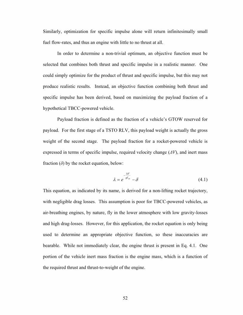
Similarly, optimization for specific impulse alone will return infinitesimally small
fuel flow-rates, and thus an engine with little to no thrust at all.
In order to determine a non-trivial optimum, an objective function must be
selected that combines both thrust and specific impulse in a realistic manner. One
could simply optimize for the product of thrust and specific impulse, but this may not
produce realistic results. Instead, an objective function combining both thrust and
specific impulse has been derived, based on maximizing the payload fraction of a
hypothetical TBCC-powered vehicle.
Payload fraction is defined as the fraction of a vehicle’s GTOW reserved for
payload. For the first stage of a TSTO RLV, this payload weight is actually the gross
weight of the second stage. The payload fraction for a rocket-powered vehicle is
expressed in terms of specific impulse, required velocity change (∆V), and inert mass
fraction (δ) by the rocket equation, below:
δλ −=∆
−spgIV
e (4.1)
This equation, as indicated by its name, is derived for a non-lifting rocket trajectory,
with negligible drag losses. This assumption is poor for TBCC-powered vehicles, as
air-breathing engines, by nature, fly in the lower atmosphere with low gravity-losses
and high drag-losses. However, for this application, the rocket equation is only being
used to determine an appropriate objective function, so these inaccuracies are
bearable. While not immediately clear, the engine thrust is present in Eq. 4.1. One
portion of the vehicle inert mass fraction is the engine mass, which is a function of
the required thrust and thrust-to-weight of the engine.
52

Assuming fixed delta-V, vehicle weight, and engine thrust-to-weight; thrust
will be constant, and the only variable in Eq. 4.1 will be specific impulse. As such,
maximizing specific impulse for a fixed value of thrust is analogous to maximizing
payload fraction. This concept is implemented in the optimizer by selecting specific
impulse alone as the objective function, and adding a constraint that thrust must be
greater than a specified limit. The same result could be found by constraining thrust
to be exactly equal to that limit; however this would retard the optimization greatly,
as the only feasible design would be one which produces that value of thrust exactly.
Optimizers tend to be more efficient when allowed to first find a feasible design, and
then approach the constraints gradually. Based on the trade-off between thrust and
specific impulse discussed above, thrust will almost always approach its lower
constraint as specific impulse approaches its maximum. The exception to this rule
occurs when other engine constraints become active first, preventing a feasible design
at the minimum engine thrust.
4.2.5 Rubber Engine
Ultimately, the results from the computer model represent a “rubber engine”
that is redesigned at every increment in Mach number to meet the input
specifications. The compression ratio, fuel-ratio(s), and bypass ratio are optimized at
each value of Mach number in order to produce the best possible performance, while
satisfying the cycle constraints. The TBE bypass duct area is also recalculated at
each design point. In a real engine, some parameters, such as the fuel flow-rates, will
change throughout the trajectory, but the compression and bypass ratios may remain
fixed, and variable geometry in the TBE bypass duct may be more difficult.
53

The thrust is also normalized by inlet mass flow so that, for a given
configuration, any size engine will produce the same performance. For a real engine,
thrust would, of course, scale with inlet area and mass flow. Specific impulse, as
indicated by Eq. 3.8, is independent of engine size. The component cross-sectional
areas of the TBE are also normalized by the inlet area of the engine. This produces a
dimensionless engine, whose results may be applied to TBCC engines in any
application.
54

CHAPTER 5: OPTIMIZATION RESULTS
The TBCC flowpaths are optimized using the computer model of Chap. 4.
The code is run on a notebook PC with a 1200MHz Pentium III processor, 512MB of
RAM, running SUSE Linux 9.1 Pro. A single engine run, repeated from Mach 0 to
4.25 by increments of 0.05, takes approximately 20-60 minutes to complete,
depending on the cycle and convergence. Many of the engine parameters remain
constant for every engine in question, and will be given in the following section.
Trade studies for the individual engines, however, involve different parameter values
for each engine, which will precede the results in the corresponding section. Finally,
the separate engines are compared directly to determine the most suitable for the first
stage of a TSTO vehicle.
5.1 Input Conditions
The TBCC flowpaths have been originally analyzed for Mach numbers from
0-5, representing the regime of a non-scramjet first stage vehicle. However, for
reasons to be discussed shortly, only the RJ can produce feasible designs above Mach
4.25. As such, results for all other engines are only given from Mach 0-4.25. All
engines are optimized for both hydrocarbon and hydrogen fuel, which, unless
specified otherwise, is assumed to be injected at 200K. This value was chosen
somewhat arbitrarily and will be varied in trade studies for each engine type. The
temperature limits for the compressor, turbine, and afterburner are assumed to be
55

1000K, 2000K, and 2200K, respectively. These values have been given as reasonable
limits of modern technology by contacts at NASA Glenn Research Center. As a
baseline, the compressor and turbine efficiencies are assumed to be 88% and 90%,
respectively. These values have been chosen as reasonable estimates, and will also be
subject to trade studies for each engine, in order to determine the importance of
knowing the exact component efficiency for each engine. The inlet wedge half-angle
is chosen arbitrarily to be 12 degrees. To allow for even comparison, all engines in
this project share the same inlet design. It should also be noted that this angle does
not represent and optimum design; it is simply chosen to allow the TBCC flowpaths
to operate across a wide range of Mach numbers and provide a basis for comparison
between the flowpaths.
The value of the minimum normalized thrust constraint has been chosen to be
3.5. This value is chosen because it is generally achievable by all candidate engines
and corresponds to reasonable specific impulse for almost all candidates. For
reference, the normalized thrust of a Space Shuttle main engine, as calculated from
data in Ref. 32, is approximately 10. It should be noted that almost every engine
cannot satisfy this constraint above approximately Mach 3.5-4.0, but higher or lower
constraint values have proven even more difficult for every engine to meet in
preliminary tests. Results corresponding to Mach numbers where this constraint is
violated will not be optimized fully, and thus cannot be compared directly. These
computationally “infeasible” designs, however, can still physically operate, just at
lower thrust levels. This is different from the other constraints, which define the
physical limits of engine operation.
56

5.2 TBE Trade Studies
Despite being the most traditional and common form of TBCC engine, the
TBE is the most complicated, analytically, of all engines studied. It requires
compressor, bypass, burner fuel, and afterburner fuel ratios to be specified as design
variables. It also requires assumed values for compressor staging ratio, compressor
and turbine efficiency, and fuel inlet temperature. Ultimately, these design variables
and component constants provide a wide and complex design space across which
many trade studies may be performed. The parameters of most interest, however, are
bypass ratio, compressor staging ratio, compressor and turbine efficiencies, and fuel
inlet temperature; as such, they will be the focus of several trade studies on TBE
performance.
5.2.1 Bypass Ratio
Bypass ratio is the most important parameter for defining TBE performance,
and as such, makes for the most interesting trade study. Holding all other conditions
constant, several TBE cases are run with different fixed and variable bypass ratio
values. For the fixed cases, the only design variables are the compression ratio,
burner fuel-air equivalence ratio, and afterburner fuel-air equivalence ratio. For the
variable bypass case, bypass ratio is optimized as a design variable as well. For all
cases, the compressor staging ratio is assumed to be 0.33, so that the bypass flow
undergoes one third of the total engine compression before being diverted around the
engine core. As such, the compressor must be able to operate across the entire flight
range, requiring some amount of core engine flow. To account for this, the maximum
allowable bypass ratio has been set at 0.95, preventing full ramjet operation. The
57

exact input values for each run are given in Table 5.1 and the results for specific
impulse, thrust, bypass ratio, compression ratio, and the burner and afterburner fuel-
air equivalence ratio are given in Figs. 5.1-5.6, respectively.
Table 5.1: TBE bypass ratio trade study input parameters Run min
M max M ∆M min
πc
max πc
min ΦB
max ΦB
min α
max α
min ΦAB
max ΦAB
fuel
TBE1 0 4.26 0.05 1 40 0.001 1 0.001 0.95 0.001 1 HC
TBE2 0 4.26 0.05 1 40 0.001 1 0.001 0.95 0.001 1 H2
TBE3 0 4.26 0.05 1 40 0.001 1 0.250 0.25 0.001 1 HC
TBE4 0 4.26 0.05 1 40 0.001 1 0.250 0.25 0.001 1 H2
TBE5 0 4.26 0.05 1 40 0.001 1 0.500 0.50 0.001 1 HC
TBE6 0 4.26 0.05 1 40 0.001 1 0.500 0.50 0.001 1 H2
TBE7 0 4.26 0.05 1 40 0.001 1 0.750 0.75 0.001 1 HC
TBE8 0 4.26 0.05 1 40 0.001 1 0.750 0.75 0.001 1 H2
ecifi
cIm
puls
e(s
ec)
4000
6000
8000
10000
12000
TBE - H2, T_fTBE - H2, T_fTBE - H2, T_fTBE - H2, T_fTBE - H2, T_f
Spe
cific
Impu
lse
(sec
)
1500
2000
2500
3000
3500
4000
4500
5000
TBE - HC, T_fuel=TBE - HC, T_fuel=TBE - HC, T_fuel=TBE - HC, T_fuel=TBE - HC, T_fuel=TBE - HC, -2sTBE - HC, +2s
10000
12000
4500
50005000
Bur
nerE
quiv
.Rat
io
0.2
0.4
0.6
0.8
1
1.2
1.4TBE - HC, a=opt.TBE - HC, a=0.25TBE - HC, a=0.50TBE - HC, a=0.75TBE - H2, a=opt.TBE - H2, a=0.25TBE - H2, a=0.50TBE - H2, a=075
M h
Byp
ass
Rat
io
0 1 2 3 40
0.2
0.4
0.6
0.8
1
1.2
1.4
TBE - HC, a=opt.TBE - HC, a=0.25TBE - HC, a=0.50TBE - HC, a=0.75TBE - H2, a=opt.TBE - H2, a=0.25TBE - H2, a=0.50TBE - H2, a=0.75
Mach0 1 2 3 4
TBE - HC, B=1.0, a=opt.TBE - H2, B=0.0, a=opt.TBE - H2, B=0.33, a=opt.TBE - H2, B=0.66, a=opt.TBE - H2, B=1.0, a=opt.
Mach
q
0 1 2 3 40
0.2
0.4
0.6
0.8
1 TBE - HC, B=0.66, a=opt.TBE - HC, B=1.0, a=opt.TBE - H2, B=0.0, a=opt.TBE - H2, B=0.33, a=opt.TBE - H2, B=0.66, a=opt.TBE - H2, B=1.0, a=opt.
Mach1 2 3 4
TBE - H2, B=0.66, a=opt.TBE - H2, B=1.0, a=opt.
Mach
Spe
cific
Impu
lse
(sec
)
0 1 2 3 40
2000
4000
6000
8000
10000
12000
TBE - HC, a=opt.TBE - HC, a=0.25TBE - HC, a=0.50TBE - HC, a=0.75TBE - H2, a=opt.TBE - H2, a=0.25TBE - H2, a=0.50TBE - H2, a=0.75
Figure 5.1: Specific impulse vs. Mach for TBE
with fixed and variable bypass ratios
58

Com
pres
orP
ress
ure
Rat
io
0 1 2 3 40
10
20
30
40
TBE - HC, a=opt.TBE - HC, a=0.25TBE - HC, a=0.50TBE - HC, a=0.75TBE - H2, a=opt.TBE - H2, a=0.25TBE - H2, a=0.50TBE - H2, a=0.75
Afte
rbur
nerE
quiv
.Rat
io
0.2
0.4
0.6
0.8
1
1.2
1.4
TBE - HC, a=opt.TBE - HC, a=0.25TBE - HC, a=0.50TBE - HC, a=0.75TBE - H2, a=opt.TBE - H2, a=0.25TBE - H2, a=0.50TBE - H2, a=0.75
Spe
cific
Impu
lse
(sec
)
2800
2900
3000
3100
3200
TBE - HC, T_fuel=2TBE - HC, T_fuel=3TBE - HC, T_fuel=4TBE - HC, T_fuel=5TBE - HC, T_fuel=1TBE - HC, -2sTBE - HC, +2s
ecifi
cIm
puls
e(s
ec)
7000
7500
8000TBE - H2, TTBE - H2, TTBE - H2, TTBE - H2, TTBE - H2, T
TBE - HCTJ - HCRJ - HC
TBE, etaT=0.85TBE, etaT=0.88TBE etaC=0 83
43000
3000
Mach1 2 3 4
TBE - HC, B=0.0, a=opt.TBE - HC, B=0.33, a=opt.TBE - HC, B=0.66, a=opt.TBE - HC, B=1.0, a=opt.TBE - H2, B=0.0, a=opt.TBE - H2, B=0.33, a=opt.TBE - H2, B=0.66, a=opt.TBE - H2, B=1.0, a=opt.
Mach1 2 3 4
TBE HC, B 0.0, a opt.TBE - HC, B=0.33, a=opt.TBE - HC, B=0.66, a=opt.TBE - HC, B=1.0, a=opt.TBE - H2, B=0.0, a=opt.TBE - H2, B=0.33, a=opt.TBE - H2, B=0.66, a=opt.TBE - H2, B=1.0, a=opt.
Mach0 1 2 3 4
0
0.2
0.4
0.6
0.8
1, , p
TBE - HC, B=0.33, a=opt.TBE - HC, B=0.66, a=opt.TBE - HC, B=1.0, a=opt.TBE - H2, B=0.0, a=opt.TBE - H2, B=0.33, a=opt.TBE - H2, B=0.66, a=opt.TBE - H2, B=1.0, a=opt.
Mach
Nor
mal
ized
Thru
st
0 1 2 3 40
1
2
3
4
TBE - HC, a=opt.TBE - HC, a=0.25TBE - HC, a=0.50TBE - HC, a=0.75TBE - H2, a=opt.TBE - H2, a=0.25TBE - H2, a=0.50TBE - H2, a=0.75
Tmin
Figure 5.2: Thrust vs. Mach for TBE with fixed and variable bypass ratios
Spe
cific
Impu
lse
(sec
)
4000
6000
8000
10000
12000
TBE - H2, T_fuel=TBE - H2, T_fuel=TBE - H2, T_fuel=TBE - H2, T_fuel=TBE - H2, T_fuel=
Spe
cific
Impu
lse
(sec
)
1000
1500
2000
2500
3000
3500
4000
4500
5000
TBE - HC, T_fuel=200TBE - HC, T_fuel=300TBE - HC, T_fuel=400TBE - HC, T_fuel=500TBE - HC, T_fuel=100TBE - HC, -2sTBE - HC, +2s
10000
12000
4000
4500
5000
4500
5000
Mach1 2 3 4
Mach1 2 3 4
TBE - H2, B=0.33, a=opt.TBE - H2, B=0.66, a=opt.TBE - H2, B=1.0, a=opt.
Mach0 1 2 3 4
TBE - HC, B=1.0, a=opt.TBE - H2, B=0.0, a=opt.TBE - H2, B=0.33, a=opt.TBE - H2, B=0.66, a=opt.TBE - H2, B=1.0, a=opt.
Nor
mal
ized
Thru
Bur
nerE
quiv
.Rat
io
0 1 2 3 40
0.2
0.4
0.6
0.8
1
1.2
1.4TBE - HC, a=opt.TBE - HC, a=0.25TBE - HC, a=0.50TBE - HC, a=0.75TBE - H2, a=opt.TBE - H2, a=0.25TBE - H2, a=0.50TBE - H2, a=075
Mach0 1 2 3 4
0
2000
4000
6000
8000
10000
12000
TBE - HC, a=opt.TBE - HC, a=0.25TBE - HC, a=0.50TBE - HC, a=0.75TBE - H2, a=opt.TBE - H2, a=0.25TBE - H2, a=0.50TBE - H2, a=0.75
Mach
Byp
ass
Rat
io
0 1 2 3 40
0.2
0.4
0.6
0.8
1
1.2
1.4
TBE - HC, a=opt.TBE - HC, a=0.25TBE - HC, a=0.50TBE - HC, a=0.75TBE - H2, a=opt.TBE - H2, a=0.25TBE - H2, a=0.50TBE - H2, a=0.75
Figure 5.3: Bypass ratio vs. Mach for TBE
with fixed and variable bypass ratios
59

Afte
rbur
nerE
quiv
.Rat
io
0 1 2 3 40
0.2
0.4
0.6
0.8
1
1.2
1.4
TBE - HC, a=opt.TBE - HC, a=0.25TBE - HC, a=0.50TBE - HC, a=0.75TBE - H2, a=opt.TBE - H2, a=0.25TBE - H2, a=0.50TBE - H2, a=0.75
Spe
cific
Impu
lse
(sec
)
2800
2900
3000
3100
3200
TBE - HC, T_fuel=200KTBE - HC, T_fuel=300KTBE - HC, T_fuel=400KTBE - HC, T_fuel=500KTBE - HC, T_fuel=1000KTBE - HC, -2sTBE - HC, +2s
Spe
cific
Impu
lse
(sec
)
7000
7500
8000TBE - H2, T_fueTBE - H2, T_fueTBE - H2, T_fueTBE - H2, T_fueTBE - H2, T_fue
TBE - HCTJ - HCRJ - HCTBE - H2TJ H2
TBE, etaT=0.85TBE, etaT=0.88TBE, etaT=0.89TBE etaT=0 90
TBE, etaC=0.83TBE, etaC=0.86TBE t C 0 87 3
43000
3000
Mach1 2 3 4
TBE - HC, B=0.0, a=opt.TBE - HC, B=0.33, a=opt.TBE - HC, B=0.66, a=opt.TBE - HC, B=1.0, a=opt.TBE - H2, B=0.0, a=opt.TBE - H2, B=0.33, a=opt.TBE - H2, B=0.66, a=opt.TBE - H2, B=1.0, a=opt.
Mach1 2 3 4
TBE - HC, B=0.66, a=opt.TBE - HC, B=1.0, a=opt.TBE - H2, B=0.0, a=opt.TBE - H2, B=0.33, a=opt.TBE - H2, B=0.66, a=opt.TBE - H2, B=1.0, a=opt.
Mach1 2 3 4
TBE - HC, B=0.66, a=opt.TBE - HC, B=1.0, a=opt.TBE - H2, B=0.0, a=opt.TBE - H2, B=0.33, a=opt.TBE - H2, B=0.66, a=opt.TBE - H2, B=1.0, a=opt.
Mach0 1 2 3 4
0
1
2
3
4
TBE - HC, a=opt.TBE - HC, a=0.25TBE - HC, a=0.50TBE - HC, a=0.75TBE - H2, a=opt.TBE - H2, a=0.25TBE - H2, a=0.50TBE - H2, a=0.75
Mach
Com
pres
orP
ress
ure
Rat
io
0 1 2 3 40
10
20
30
40
TBE - HC, a=opt.TBE - HC, a=0.25TBE - HC, a=0.50TBE - HC, a=0.75TBE - H2, a=opt.TBE - H2, a=0.25TBE - H2, a=0.50TBE - H2, a=0.75
Figure 5.4: Compressor ratio vs. Mach for TBE
with fixed and variable bypass ratios
Spe
cific
Impu
lse
(sec
)
4000
6000
8000
10000
12000
TBE - H2, T_fuel=200TBE - H2, T_fuel=300TBE - H2, T_fuel=400TBE - H2, T_fuel=500TBE - H2, T_fuel=100
Spe
cific
Impu
lse
(sec
)
1000
1500
2000
2500
3000
3500
4000
4500
5000
TBE - HC, T_fuel=200KTBE - HC, T_fuel=300KTBE - HC, T_fuel=400KTBE - HC, T_fuel=500KTBE - HC, T_fuel=1000KTBE - HC, -2sTBE - HC, +2s
ec)
8000
10000
12000
4000
4500
5000
4000
4500
5000
Mach1 2 3 4
Mach1 2 3 4
, , pTBE - H2, B=1.0, a=opt.
Mach1 2 3 4
TBE - H2, B=0.33, a=opt.TBE - H2, B=0.66, a=opt.TBE - H2, B=1.0, a=opt.
Nor
mal
ized
T
00
1
2
Com
pres
orP
ress
ure
Mach0 1 2 3 4
0
00
00
00
00
00
TBE - HC, a=opt.TBE - HC, a=0.25TBE - HC, a=0.50TBE - HC, a=0.75TBE - H2, a=opt.TBE - H2, a=0.25TBE - H2, a=0.50TBE - H2, a=0.75
Mach
yp
0 1 2 3 40
0.2
0.4
0.6
0.8
1
1.2
TBE - HC, a=opt.TBE - HC, a=0.25TBE - HC, a=0.50TBE - HC, a=0.75TBE - H2, a=opt.TBE - H2, a=0.25TBE - H2, a=0.50TBE - H2, a=0.75
Mach
Bur
nerE
quiv
.Rat
io
0 1 2 3 40
0.2
0.4
0.6
0.8
1
1.2
1.4TBE - HC, a=opt.TBE - HC, a=0.25TBE - HC, a=0.50TBE - HC, a=0.75TBE - H2, a=opt.TBE - H2, a=0.25TBE - H2, a=0.50TBE - H2, a=075
Figure 5.5: Burner equivalence ratio vs. Mach for TBE
with fixed and variable bypass ratios
60
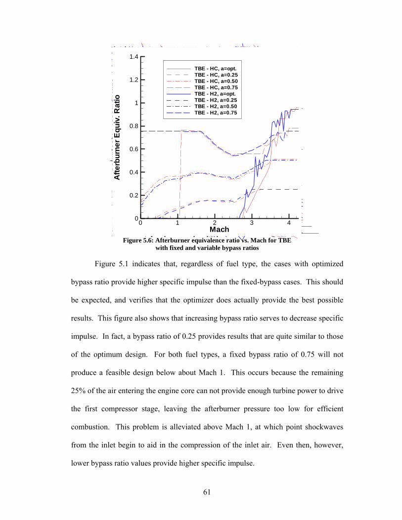
Spe
cific
Impu
lse
(sec
)
2700
2800
2900
3000
3100
3200
TBE - HC, T_fuel=200KTBE - HC, T_fuel=300KTBE - HC, T_fuel=400KTBE - HC, T_fuel=500KTBE - HC, T_fuel=1000KTBE - HC, -2sTBE - HC, +2s
Spe
cific
Impu
lse
(sec
)
7000
7500
8000TBE - H2, T_fuel=20TBE - H2, T_fuel=30TBE - H2, T_fuel=40TBE - H2, T_fuel=50TBE - H2, T_fuel=10
TBE - HCTJ - HCRJ - HCTBE - H2TJ - H2RJ - H2
E, etaT=0.85E, etaT=0.88E, etaT=0.89E, etaT=0.90E, etaT=0.91E etaT=0 92
TBE, etaC=0.83TBE, etaC=0.86TBE, etaC=0.87TBE, etaC=0.88 st
3
4) 2900
30003000
Mach1 2 3 4
, , pTBE - HC, B=0.66, a=opt.TBE - HC, B=1.0, a=opt.TBE - H2, B=0.0, a=opt.TBE - H2, B=0.33, a=opt.TBE - H2, B=0.66, a=opt.TBE - H2, B=1.0, a=opt.
Mach1 2 3 4
TBE - H2, B=0.0, a=opt.TBE - H2, B=0.33, a=opt.TBE - H2, B=0.66, a=opt.TBE - H2, B=1.0, a=opt.
Mach1 2 3 4
TBE - H2, B=0.0, a=opt.TBE - H2, B=0.33, a=opt.TBE - H2, B=0.66, a=opt.TBE - H2, B=1.0, a=opt.
Mach0 1 2 3 4
TBE - HC, a=opt.TBE - HC, a=0.25TBE - HC, a=0.50TBE - HC, a=0.75TBE - H2, a=opt.TBE - H2, a=0.25TBE - H2, a=0.50TBE - H2, a=0.75
Mach
Com
pres
orP
ress
ure
Rat
io
0 1 2 3 40
10
20
30
TBE - HC, a=opt.TBE - HC, a=0.25TBE - HC, a=0.50TBE - HC, a=0.75TBE - H2, a=opt.TBE - H2, a=0.25TBE - H2, a=0.50TBE - H2, a=0.75
Mach
Afte
rbur
nerE
quiv
.Rat
io
0 1 2 3 40
0.2
0.4
0.6
0.8
1
1.2
1.4
TBE - HC, a=opt.TBE - HC, a=0.25TBE - HC, a=0.50TBE - HC, a=0.75TBE - H2, a=opt.TBE - H2, a=0.25TBE - H2, a=0.50TBE - H2, a=0.75
Figure 5.6: Afterburner equivalence ratio vs. Mach for TBE
with fixed and variable bypass ratios
Figure 5.1 indicates that, regardless of fuel type, the cases with optimized
bypass ratio provide higher specific impulse than the fixed-bypass cases. This should
be expected, and verifies that the optimizer does actually provide the best possible
results. This figure also shows that increasing bypass ratio serves to decrease specific
impulse. In fact, a bypass ratio of 0.25 provides results that are quite similar to those
of the optimum design. For both fuel types, a fixed bypass ratio of 0.75 will not
produce a feasible design below about Mach 1. This occurs because the remaining
25% of the air entering the engine core can not provide enough turbine power to drive
the first compressor stage, leaving the afterburner pressure too low for efficient
combustion. This problem is alleviated above Mach 1, at which point shockwaves
from the inlet begin to aid in the compression of the inlet air. Even then, however,
lower bypass ratio values provide higher specific impulse.
61

For the optimized and the 0.25 and 0.50 fixed-bypass cases the specific
impulse curves follow a similar trend. The curves drop relatively sharply up to about
Mach 0.75, where they then decrease more gradually up to Mach 2.5, where every
curve has a slight knee, before decreasing more steeply. Above Mach 3.0, the
optimized curve appears to cross the fixed cases, but, as indicated by Fig. 5.2, the
minimum thrust constraint is violated by the engines at this point, and a comparison
above this point cannot be made. As mentioned previously, each engine may still
perform above Mach 3.0, but with a violated constraint, the design variables cannot
be optimized properly. Also mentioned previously, results are only given up to Mach
4.25, because above this point, no engine is able to operate at all. This occurs
because the inlet air temperature is high enough that, even with a very modest
compression ratio, the assumed 1000K compressor temperature limit is violated for
any design above Mach 4.25. This violation actually occurs at the compressor exit
because, even with a small compression ratio, the compressor exit temperature is
higher than that of the compressor inlet. This is illustrated in Fig. 5.7, below, which
layers the exit temperature for a hypothetical compressor with a pressure ratio of 1.1
on top of the inlet properties from the assumed trajectory, discussed in Section 3.3.
As indicated below, even with a very small pressure ratio, the compressor exit
temperature will exceed its assumed limit at approximately Mach 4.25. As identical
trajectory and inlet models are assumed for every engine, each cycle that includes a
compressor will be limited to operation below Mach 4.25.
62

Mach
Com
pres
sorI
nlet
and
Exi
tTem
pera
ture
(K)
0 1 2 3 40
200
400
600
800
1000
1200
T2 (K)T3 (K)
Figure 5.7: Compressor inlet and exit temperature
vs. Mach number for a compression ratio of 1.1
Figures 5.3-5.6 show the design variable values for each optimization run in
this trade study. Figure 5.3 shows that the optimal bypass ratio is approximately 0.0
below Mach 2.5, which corresponds to the knee in the specific impulse curve. At this
point, in order maintain a feasible design, the bypass ratio must increase. Figure 5.4
shows that, as discussed above, larger bypass ratio values cannot provide higher
compression ratios, because they correspond to lower mass-flow through the turbine.
Thus, as the bypass ratio is increased, the compressor pressure ratio must decrease.
Also note that the compression ratio curves are almost identical for both fuel types,
which makes sense as no fuel is introduced upstream of the of the compressor, and
the turbine is subject to the same temperature limit regardless of fuel. Figure 5.5
indicates that the burner equivalence ratio changes very slightly across the flight
range for each combination of fuel type and bypass ratio. All cases require fuel lean
63

combustion in order to satisfy the turbine inlet temperature constraint. Finally, Fig.
5.6 shows that, as might be expected by the constraint of Eq. 2.13, the afterburner
equivalence ratio for each case generally follows the corresponding curve of bypass
ratio.
The jaggedness in the curves for each design variable is an artifact of the DOT
optimizer. With four design variables, several constraints with small gradients, and a
design space with several local optima, the optimizer can find many combinations of
design variable values that provide very similar results for specific impulse. The
optimization scheme has been designed to provide smooth curves in the objective
function, but a more sophisticated optimizer is required to provide smooth transitions
in the design variable values, while also allowing the optimizer to determine the
global optimum. Additionally, any design variable values above Mach 3.0 are not
fully optimized as the thrust constraint is generally violated above that point.
5.2.2 Compressor Staging Ratio
The results presented above assume a compressor staging ratio of 0.33 for
every optimization run. This particular value is chosen somewhat arbitrarily, so it is
of interest to assess the impact of changing it. To investigate the impact of
compressor staging ratio, several TBE runs are also optimized with fixed compressor
staging ratio values of 0.0, 0.66, and 1.0. The baseline design variable limits, given
as runs “TBE1” and “TBE2” in Table 5.1, are used for every optimization run in this
study. As before, Figs. 5.8-5.13 demonstrate how specific impulse, thrust, and the
four design variables vary with freestream Mach number and the compressor staging
ratio.
64

ec)
10000
12000(s
ec)
3500
4000
4500
5000
TBETBETBETBETBETBETBE
nerE
quiv
.Rat
io
0.6
0.8
1
1.2
1.4TBE - HC,TBE - HC,TBE - HC,TBE - HC,TBE - H2,TBE - H2,TBE - H2,TBE - H2,
Byp
ass
Rat
io
0.6
0.8
1
1.2
1.4
TBE - HC, a=opt.TBE - HC, a=0.25TBE - HC, a=0.50TBE - HC, a=0.75TBE - H2, a=opt.TBE - H2, a=0.25TBE - H2, a=0.50TBE - H2, a=0.75
Spe
cific
Impu
lse
(sec
)
4000
6000
8000
10000
12000
TBE - HC, a=opt.TBE - HC, a=0.25TBE - HC, a=0.50TBE - HC, a=0.75TBE - H2, a=opt.TBE - H2, a=0.25TBE - H2, a=0.50TBE - H2, a=0.75B
ypas
sR
atio
0 1 2 3 40
0.2
0.4
0.6
0.8
1
1.2
TBE - HC, B=0.0, a=opt.TBE - HC, B=0.33, a=opt.TBE - HC, B=0.66, a=opt.TBE - HC, B=1.0, a=opt.TBE - H2, B=0.0, a=opt.TBE - H2, B=0.33, a=opt.TBE - H2, B=0.66, a=opt.TBE - H2, B=1.0, a=opt.
Bur
nerE
quiv
.Rat
io
0.2
0.4
0.6
0.8
1
1.2
TBE - HC, B=0.0, a=opt.TBE - HC, B=0.33, a=opt.TBE - HC, B=0.66, a=opt.TBE - HC, B=1.0, a=opt.TBE - H2, B=0.0, a=opt.TBE - H2, B=0.33, a=opt.TBE - H2, B=0.66, a=opt.TBE - H2, B=1.0, a=opt.
Mach
Spe
cific
Impu
lse
(sec
)
0 1 2 3 40
2000
4000
6000
8000
10000
12000TBE - HC, B=0.0, a=opt.TBE - HC, B=0.33, a=opt.TBE - HC, B=0.66, a=opt.TBE - HC, B=1.0, a=opt.TBE - H2, B=0.0, a=opt.TBE - H2, B=0.33, a=opt.TBE - H2, B=0.66, a=opt.TBE - H2, B=1.0, a=opt.
Figure 5.8: Specific impulse vs. Mach for TBE
with fixed compressor staging ratios
Com
pres
orP
ress
ure
Rat
io
0 1 2 3 40
10
20
30
40
TBE - HC, B=0.0, a=opt.TBE - HC, B=0.33, a=opt.TBE - HC, B=0.66, a=opt.TBE - HC, B=1.0, a=opt.TBE - H2, B=0.0, a=opt.TBE - H2, B=0.33, a=opt.TBE - H2, B=0.66, a=opt.TBE - H2, B=1.0, a=opt.
Afte
rbur
nerE
quiv
.Rat
io
0.2
0.4
0.6
0.8
1
1.2
TBE - HC, B=0.0, a=opt.TBE - HC, B=0.33, a=opt.TBE - HC, B=0.66, a=opt.TBE - HC, B=1.0, a=opt.TBE - H2, B=0.0, a=opt.TBE - H2, B=0.33, a=opt.TBE - H2, B=0.66, a=opt.TBE - H2, B=1.0, a=opt.
Nor
mal
ized
Thru
st
1
2
3
4
TBE - HC, a=opt.TBE - HC, a=0.25TBE - HC, a=0.50TBE - HC, a=0.75TBE - H2, a=opt.TBE - H2, a=0.25TBE - H2, a=0.50TBE - H2, a=0.75
mpr
esor
Pre
ssur
eR
atio
20
30
40
TBE - HC, aTBE - HC, aTBE - HC, aTBE - HC, aTBE - H2, aTBE - H2, aTBE - H2, aTBE - H2, a
urne
rEqu
iv.R
atio
0.6
0.8
1
1.2
1.4
TBE - HC, a=opt.TBE - HC, a=0.25TBE - HC, a=0.50TBE - HC, a=0.75TBE - H2, a=opt.TBE - H2, a=0.25TBE - H2, a=0.50TBE - H2, a=0.75
_fuel=200K_fuel=300K_fuel=400K_fuel=500K_fuel=1000K
(sec
)
3000
3100
3200
TBE -TBE -TBE -TBE -TBE -TBE -TBE -ec
) 7500
8000l=200Kl=300Kl=400Kl=500Kl=1000K
Mach
Nor
mal
ized
Thru
st
0 1 2 3 40
1
2
3
4
TBE - HC, B=0.0, a=opt.TBE - HC, B=0.33, a=opt.TBE - HC, B=0.66, a=opt.TBE - HC, B=1.0, a=opt.TBE - H2, B=0.0, a=opt.TBE - H2, B=0.33, a=opt.TBE - H2, B=0.66, a=opt.TBE - H2, B=1.0, a=opt.
Tmin
Figure 5.9: Thrust vs. Mach for TBE with fixed compressor staging ratios
65
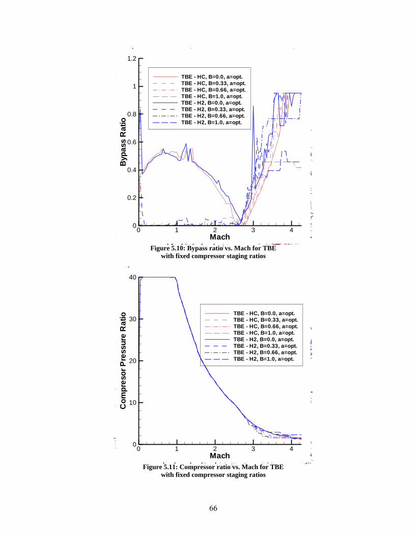
(sec
)
8000
10000
12000
TBETBETBETBETBE
ulse
(sec
)
3000
3500
4000
4500
5000
TBE - HTBE - HTBE - HTBE - HTBE - HTBE - HTBE - H
Bur
nerE
quiv
.Rat
io
0 1 2 3 40
0.2
0.4
0.6
0.8
1
1.2
TBE - HC, B=0.0, a=opt.TBE - HC, B=0.33, a=opt.TBE - HC, B=0.66, a=opt.TBE - HC, B=1.0, a=opt.TBE - H2, B=0.0, a=opt.TBE - H2, B=0.33, a=opt.TBE - H2, B=0.66, a=opt.TBE - H2, B=1.0, a=opt.
Bur
nerE
quiv
.Rat
io
0.6
0.8
1
1.2
1.4TBE - HC, a=opTBE - HC, a=0.TBE - HC, a=0.TBE - HC, a=0.TBE - H2, a=opTBE - H2, a=0.TBE - H2, a=0.TBE - H2, a=07
Byp
ass
Rat
io
0.4
0.6
0.8
1
1.2
1.4
TBE - HC, a=opt.TBE - HC, a=0.25TBE - HC, a=0.50TBE - HC, a=0.75TBE - H2, a=opt.TBE - H2, a=0.25TBE - H2, a=0.50TBE - H2, a=0.75
Spe
cific
Impu
lse
(sec
)
2000
4000
6000
8000
10000
12000
TBE - HC, a=opt.TBE - HC, a=0.25TBE - HC, a=0.50TBE - HC, a=0.75TBE - H2, a=opt.TBE - H2, a=0.25TBE - H2, a=0.50TBE - H2, a=0.75
Mach0 1 2 3 4
0
2000
4000
6000
8000
0000
TBE - HC, B=0.0, a=opt.TBE - HC, B=0.33, a=opt.TBE - HC, B=0.66, a=opt.TBE - HC, B=1.0, a=opt.TBE - H2, B=0.0, a=opt.TBE - H2, B=0.33, a=opt.TBE - H2, B=0.66, a=opt.TBE - H2, B=1.0, a=opt.
Mach
Byp
ass
Rat
io
0 1 2 3 40
0.2
0.4
0.6
0.8
1
1.2
TBE - HC, B=0.0, a=opt.TBE - HC, B=0.33, a=opt.TBE - HC, B=0.66, a=opt.TBE - HC, B=1.0, a=opt.TBE - H2, B=0.0, a=opt.TBE - H2, B=0.33, a=opt.TBE - H2, B=0.66, a=opt.TBE - H2, B=1.0, a=opt.
Figure 5.10: Bypass ratio vs. Mach for TBE
with fixed compressor staging ratios
Nor
mal
ized
Thru
st
1
2
3
4
TBE - HC, a=opt.TBE - HC, a=0.25TBE - HC, a=0.50TBE - HC, a=0.75TBE - H2, a=opt.TBE - H2, a=0.25TBE - H2, a=0.50TBE - H2, a=0.75
Com
pres
orP
ress
ure
Rat
io
10
20
30
40
TBE - HC, a=opTBE - HC, a=0.2TBE - HC, a=0.5TBE - HC, a=0.7TBE - H2, a=opTBE - H2, a=0.2TBE - H2, a=0.5TBE - H2, a=0.7
erbu
rner
Equ
iv.R
atio
0.6
0.8
1
1.2
1.4
TBE - HC, a=opt.TBE - HC, a=0.25TBE - HC, a=0.50TBE - HC, a=0.75TBE - H2, a=opt.TBE - H2, a=0.25TBE - H2, a=0.50TBE - H2, a=0.75
l=200Kl=300Kl=400Kl=500Kl=1000K
ulse
(sec
)
3000
3100
3200
TBE - HCTBE - HCTBE - HCTBE - HCTBE - HCTBE - HCTBE - HC
(sec
) 7500
8000
TTTTT
00K00K00K00K000K
Afte
rbur
nerE
quiv
.Rat
io
0 1 2 3 40
0.2
0.4
0.6
0.8
1
1.2
TBE - HC, B=0.0, a=opt.TBE - HC, B=0.33, a=opt.TBE - HC, B=0.66, a=opt.TBE - HC, B=1.0, a=opt.TBE - H2, B=0.0, a=opt.TBE - H2, B=0.33, a=opt.TBE - H2, B=0.66, a=opt.TBE - H2, B=1.0, a=opt.
Mach
oa
edus
t
0 1 2 3 40
1
2
3
4
TBE - HC, B=0.0, a=opt.TBE - HC, B=0.33, a=opt.TBE - HC, B=0.66, a=opt.TBE - HC, B=1.0, a=opt.TBE - H2, B=0.0, a=opt.TBE - H2, B=0.33, a=opt.TBE - H2, B=0.66, a=opt.TBE - H2, B=1.0, a=opt.
Mach
Com
pres
orP
ress
ure
Rat
io
0 1 2 3 40
10
20
30
40
TBE - HC, B=0.0, a=opt.TBE - HC, B=0.33, a=opt.TBE - HC, B=0.66, a=opt.TBE - HC, B=1.0, a=opt.TBE - H2, B=0.0, a=opt.TBE - H2, B=0.33, a=opt.TBE - H2, B=0.66, a=opt.TBE - H2, B=1.0, a=opt.
Figure 5.11: Compressor ratio vs. Mach for TBE
with fixed compressor staging ratios
66

ulse
(sec
)
8000
10000
12000
TBE - H2TBE - H2TBE - H2TBE - H2TBE - H2
mpu
lse
(sec
)
2500
3000
3500
4000
4500
5000
TBE - HC, T_TBE - HC, T_TBE - HC, T_TBE - HC, T_TBE - HC, T_TBE - HC, -2sTBE - HC, +2
Bur
nerE
quiv
.Rat
io
0.4
0.6
0.8
1
1.2
1.4TBE - HC, a=opt.TBE - HC, a=0.25TBE - HC, a=0.50TBE - HC, a=0.75TBE - H2, a=opt.TBE - H2, a=0.25TBE - H2, a=0.50TBE - H2, a=075
Byp
ass
Rat
io
0.4
0.6
0.8
1
1.2
1.4
TBE - HC, a=opt.TBE - HC, a=0.25TBE - HC, a=0.50TBE - HC, a=0.75TBE - H2, a=opt.TBE - H2, a=0.25TBE - H2, a=0.50TBE - H2, a=0.75
Spe
cific
Impu
lse
(sec
)
2000
4000
6000
8000
10000
12000
TBE - HC, a=opt.TBE - HC, a=0.25TBE - HC, a=0.50TBE - HC, a=0.75TBE - H2, a=opt.TBE - H2, a=0.25TBE - H2, a=0.50TBE - H2, a=0.75
Mach0 1 2 3 4
0
0
0
0
0
0
TBE - HC, B=0.33, a=opt.TBE - HC, B=0.66, a=opt.TBE - HC, B=1.0, a=opt.TBE - H2, B=0.0, a=opt.TBE - H2, B=0.33, a=opt.TBE - H2, B=0.66, a=opt.TBE - H2, B=1.0, a=opt.
Mach0 1 2 3 4
0
0.2
0.4
0.6
0.8
1
1.2
TBE - HC, B=0.0, a=opt.TBE - HC, B=0.33, a=opt.TBE - HC, B=0.66, a=opt.TBE - HC, B=1.0, a=opt.TBE - H2, B=0.0, a=opt.TBE - H2, B=0.33, a=opt.TBE - H2, B=0.66, a=opt.TBE - H2, B=1.0, a=opt.
Mach
Bur
nerE
quiv
.Rat
io
0 1 2 3 40
0.2
0.4
0.6
0.8
1
1.2
TBE - HC, B=0.0, a=opt.TBE - HC, B=0.33, a=opt.TBE - HC, B=0.66, a=opt.TBE - HC, B=1.0, a=opt.TBE - H2, B=0.0, a=opt.TBE - H2, B=0.33, a=opt.TBE - H2, B=0.66, a=opt.TBE - H2, B=1.0, a=opt.
Figure 5.12: Burner equivalence ratio vs. Mach for TBE
with fixed compressor staging ratios
Nor
mal
ized
Thru
st
1
2
3
4
TBE - HC, a=opt.TBE - HC, a=0.25TBE - HC, a=0.50TBE - HC, a=0.75TBE - H2, a=opt.TBE - H2, a=0.25TBE - H2, a=0.50TBE - H2, a=0.75
Com
pres
orP
ress
ure
Rat
io
10
20
30
40
TBE - HC, a=opt.TBE - HC, a=0.25TBE - HC, a=0.50TBE - HC, a=0.75TBE - H2, a=opt.TBE - H2, a=0.25TBE - H2, a=0.50TBE - H2, a=0.75
Afte
rbur
nerE
quiv
.Rat
io
0.4
0.6
0.8
1
1.2
1.4
TBE - HC, a=opt.TBE - HC, a=0.25TBE - HC, a=0.50TBE - HC, a=0.75TBE - H2, a=opt.TBE - H2, a=0.25TBE - H2, a=0.50TBE - H2, a=0.75
0K0K0K0K00K
mpu
lse
(sec
)
2900
3000
3100
3200
TBE - HC, T_fuTBE - HC, T_fuTBE - HC, T_fuTBE - HC, T_fuTBE - HC, T_fuTBE - HC, -2sTBE - HC, +2s
ulse
(sec
) 7500
8000
TBE -TBE -TBE -TBE -TBE -
Mach0 1 2 3 4
TBE - HC, B=0.0, a=opt.TBE - HC, B=0.33, a=opt.TBE - HC, B=0.66, a=opt.TBE - HC, B=1.0, a=opt.TBE - H2, B=0.0, a=opt.TBE - H2, B=0.33, a=opt.TBE - H2, B=0.66, a=opt.TBE - H2, B=1.0, a=opt.
Mach0 1 2 3 4
0
10
20
30
40
TBE - HC, B=0.0, a=opt.TBE - HC, B=0.33, a=opt.TBE - HC, B=0.66, a=opt.TBE - HC, B=1.0, a=opt.TBE - H2, B=0.0, a=opt.TBE - H2, B=0.33, a=opt.TBE - H2, B=0.66, a=opt.TBE - H2, B=1.0, a=opt.
Mach
Afte
rbur
nerE
quiv
.Rat
io
0 1 2 3 40
0.2
0.4
0.6
0.8
1
1.2
TBE - HC, B=0.0, a=opt.TBE - HC, B=0.33, a=opt.TBE - HC, B=0.66, a=opt.TBE - HC, B=1.0, a=opt.TBE - H2, B=0.0, a=opt.TBE - H2, B=0.33, a=opt.TBE - H2, B=0.66, a=opt.TBE - H2, B=1.0, a=opt.
Figure 5.13: Afterburner equivalence ratio vs. Mach for TBE
with fixed compressor staging ratios
67

Figure 5.8 indicates the interesting result that, as long as a fan stage is utilized
to some extent, it does not matter how the compression is divided between the two
stages. The specific impulse curves for all non-zero staging ratios are essentially
identical, and are substantially greater than the βc=0.0 curves. Fuel type does not
appear to play a part in compressor staging, beyond the results shown above that
hydrogen fuel is able to provide much higher specific impulse than hydrocarbon,
across the entire flight range. The specific impulse curves also show the same
general trend seen before, with continually decreasing specific impulse and a knee in
the curve at about Mach 2.5.
A closer look at Figs. 5.8 and 5.9 shows that the βc=0.0 cases cannot provide a
feasible design at Mach 0. This result and the lower performance of these cases in
general can be attributed to the equal-exit velocity design for the bypass duct.
Without a fan stage to accelerate the bypass flow at Mach 0, it is impossible for the
bypass duct exit velocity to equal that of the turbine. Also, as seen in the previous
trade study, above about Mach 3, most optimization runs cannot satisfy the minimum
thrust constraint, so the specific impulse results become less clear.
Figures 5.10-5.13 verify that, for each fuel type, all non-zero compressor
staging cases provide almost identical results. Figure 5.10 shows the same optimized
bypass ratio trend seen in the previous study for the non-zero staging cases, except
that larger bypass ratio values are required below Mach 3.0 for the zero-staging cases.
Figure 5.11 indicates that, regardless of fuel type or compressor staging, identical
overall compressor pressure ratios provide the optimal specific impulse. This curve
corresponds to the maximum allowable pressure ratio at any Mach number. Below
68

Mach 1.0, the pressure ratio is at its specified upper design limit of 40. At Mach 1.0
the first inlet shockwave becomes active, and the compressor exit temperature will
exceed the 1000K limit unless the compression ratio is scaled down, as seen for all
points greater than Mach 1.0. Then, as explained in the previous study, the
compressor exit temperature will exceed 1000K for any design above Mach 4.25.
Figures 5.12 and 5.13 verify the results seen in the previous study: the burner must
operate fuel-lean at all design points to satisfy the turbine inlet temperature constraint,
and the afterburner equivalence ratio will always follow the same trend as the bypass
ratio, satisfying the constraint that only bypass air may react in the afterburner. This
also demonstrates that the afterburner actually burns stoichiometrically with the
bypass air, but the presence of non-bypass flow in the afterburner results in fuel-lean
ratios.
5.2.3 Compressor Efficiency
All TBE runs presented thus far have assumed compressor and turbine
efficiencies of 88% and 90%, respectively. These values have been chosen as
reasonable estimates of component efficiency, but it is possible that the extreme
conditions under which this engine would operate, or advances in turbomachinery
technology, could lead to lower or higher efficiencies than those assumed. Therefore,
several cases are run in order to determine the sensitivity of TBE performance to
varying component efficiency. Compressor efficiency is varied by ±5%, in small
increments, as specified in Table 5.2. For all cases, the baseline “TBE1” case is used,
allowing variable bypass ratio, fixed compressor staging at 0.33, and burning only
hydrocarbon fuel.
69

Table 5.2: TBE compressor efficiency values Run ηc
TBE9 0.93
TBE10 0.90
TBE11 0.89
TBE1 0.88
TBE12 0.87
TBE13 0.86
TBE14 0.83
In order to determine the statistical significance of variations in compressor
efficiency, a baseline control case is optimized multiple times. While not intuitively
obvious, Coleman and Steele prove that only 10 samples are required to approximate
a Gaussian distribution39. The control case assumes the baseline design variable
limits, engine parameters, and compressor and turbine efficiencies of 88% and 90%,
respectively. From these samples, an approximate 2-σ confidence interval is
calculated, accounting for numerical variability and repeatability inherent to the
optimization code. Engine performance that falls outside of this interval, therefore,
must be a result of significant change in efficiency, and not just variability in the
code.
Figures 5.14 and 5.15 show the impact of compressor efficiency on specific
impulse for the hydrocarbon-fueled TBE. Similar results should be expected for
hydrogen fuel, as the compressor operates under the same conditions for each. Figure
5.14 illustrates that, globally, variations in compressor efficiency up to 2% do not
seem to make much of a difference in specific impulse. Efficiency changes up to 5%
are more noticeable, but still follow the exact same trends. When viewing the
segment from Mach 1.5 to 2.5 more closely, though, Fig. 5.15 shows that even a 1%
change in compressor efficiency does result in a statistically significant change in
70

engine performance. As would be expected, larger compressor efficiency values lead
to increased engine performance. The contrary, of course, is also true.
In addition to demonstrating the statistical significance of changes in
compressor efficiency, the confidence interval also demonstrates the great precision
and repeatability of the optimizer. The confidence interval is at its largest at Mach
0.3, and even then, it accounts for only ±1.0% variation in specific impulse. This
interval is based solely on the repeatability of the optimizer, and does not account for
other possible sources of error in the model, such as inaccuracies in other engine
assumptions or component models. Thus, while significant on the basis of
repeatability, considering the fidelity of a quasi-1D model, a variation of 2% in
compressor efficiency should have little overall impact on the results of this study.
0 1
0
Mach2 3 4 0 1
0
00
0.2
Mach2 3 4
Spe
cif
12600
2700
2800
Spe
cific
Im
6500
7000
Mach2 3 4
Mach1 2 3 4
Mach0 1 2 3 4 5
0
00
00
00
00
00TBE - HCTJ - HCRJ - HCTBE - H2TJ - H2RJ - H2
ach3 4
Mach0 1 2 3 4
0
500
1000
1500
2000
2500
3000
3500
4000
4500
5000
TBE, etaT=0.85TBE, etaT=0.88TBE, etaT=0.89TBE, etaT=0.90TBE, etaT=0.91TBE, etaT=0.92TBE, etaT=0.95TBE, -2sTBE, +2s
Mach
Spe
cific
Impu
lse
(sec
)
0 1 2 3 40
500
1000
1500
2000
2500
3000
3500
4000
4500
5000
TBE, etaC=0.83TBE, etaC=0.86TBE, etaC=0.87TBE, etaC=0.88TBE, etaC=0.89TBE, etaC=0.90TBE, etaC=0.93TBE, -2sTBE, +2s
Figure 5.14: Specific impulse vs. Mach for TBE
with varying compressor efficiency
71

ach3 4
Mach2 3 4
Mach2 3 4
Mach1.8 2 2.2 2.4
Mach1.8 2 2.2 2.4
Mach0 1 2 3 4 5
0
1
2
3
TBE - HCTJ - HCRJ - HCTBE - H2TJ - H2RJ - H2
Mach1.6 1.8 2 2.2 2.4
2600
2700
2800
2900
3000
TBE, etaT=0.85TBE, etaT=0.88TBE, etaT=0.89TBE, etaT=0.90TBE, etaT=0.91TBE, etaT=0.92TBE, etaT=0.95TBE, -2sTBE, +2s
Mach
Spe
cific
Impu
lse
(sec
)
1.6 1.8 2 2.2 2.42600
2700
2800
2900
3000
TBE, etaC=0.83TBE, etaC=0.86TBE, etaC=0.87TBE, etaC=0.88TBE, etaC=0.89TBE, etaC=0.90TBE, etaC=0.93TBE, -2sTBE, +2s
Figure 5.15: Close-up compressor efficiency sensitivity
5.2.4 Turbine Efficiency
An identical trade study is also performed on turbine efficiency, with
variations up to ±5% as given below.
Table 5.3: TBE turbine efficiency values Run ηc
TBE15 0.95
TBE16 0.92
TBE17 0.91
TBE1 0.90
TBE18 0.89
TBE19 0.88
TBE20 0.85
As before, Figs. 5.16 and 5.17 show the variation in specific impulse with turbine
efficiency and Mach number, with an approximate 2-σ interval accounting for
repeatability in the code
72

M h
Spe
cific
Impu
lse
(sec
)
0 1 2 3 40
500
1000
1500
2000
2500
3000
3500
4000
4500
5000
TBE, etaC=0.83TBE, etaC=0.86TBE, etaC=0.87TBE, etaC=0.88TBE, etaC=0.89TBE, etaC=0.90TBE, etaC=0.93TBE, -2sTBE, +2s
0 10
Mach2 3 4 0
0
00
0.2
Mach2 3 4
Spe
cific
I
2600
2700
2800
Spe
cific
Imp
65
70
Mach1 2 3 4
Mach1 2 3 4
Mach0 1 2 3 4 5
0
2000
4000
6000
8000
10000
12000
TBE - HCTJ - HCRJ - HCTBE - H2TJ - H2RJ - H2
Mach2 3 4
Mach
Spe
cific
Impu
lse
(sec
)
0 1 2 3 40
500
1000
1500
2000
2500
3000
3500
4000
4500
5000
TBE, etaT=0.85TBE, etaT=0.88TBE, etaT=0.89TBE, etaT=0.90TBE, etaT=0.91TBE, etaT=0.92TBE, etaT=0.95TBE, -2sTBE, +2s
Figure 5.16: Specific impulse vs. Mach for TBE
with varying turbine efficiency
M h
Spe
cific
Impu
lse
(sec
)
1.6 1.8 2 2.2 2.42600
2700
2800
2900
3000
TBE, etaC=0.83TBE, etaC=0.86TBE, etaC=0.87TBE, etaC=0.88TBE, etaC=0.89TBE, etaC=0.90TBE, etaC=0.93TBE, -2sTBE, +2s
Mach2 3 4
Mach2 3 4
Mach2 3 4
Mach1.8 2 2.2 2.4
Mach6 1.8 2 2.2 2.4
Mach
oa
edus
t
0 1 2 3 4 50
1
2
3
4
TBE - HCTJ - HCRJ - HCTBE - H2TJ - H2RJ - H2
Mach
Spe
cific
Impu
lse
(sec
)
1.6 1.8 2 2.2 2.42600
2700
2800
2900
3000
TBE, etaT=0.85TBE, etaT=0.88TBE, etaT=0.89TBE, etaT=0.90TBE, etaT=0.91TBE, etaT=0.92TBE, etaT=0.95TBE, -2sTBE, +2s
Figure 5.17: Close-up of turbine efficiency sensitivity
73
Figures 5.16 and 5.17 show that, as in the compressor, a 1% variation in
efficiency produces a change in performance that is more significant than the
repeatability of the optimizer. An efficiency increase of 5%, however, still only
increases specific impulse by about 1.5%. The sensitivity of engine performance to
turbine efficiency is also less than that to compressor efficiency, which follows the
traditional expectation for a standard turbojet engine. By operating with an adverse
pressure gradient, the compressor is more sensitive to changes in efficiency than the
turbine.
5.2.5 Fuel Inlet Temperature
As mentioned earlier, a fuel inlet temperature of 200K is assumed for most
TBCC engines. This value has been selected somewhat arbitrarily, and may be quite
inaccurate for engines employing active cooling. To investigate the impact of
increases in fuel temperature, several cases are optimized with varying inlet
temperature values. For each case, all other design variables and engine parameters
maintain their baseline values (βc=0.33, ηc=88%, ηt=90%). Results are presented for
both hydrogen and hydrocarbon fuel. In addition to the baseline of 200K, fuel inlet
temperatures of 300K, 400K, 500K, and 1000K are tested, with the results shown
below.
74

Spe
cific
Impu
lse
(sec
)
0 1 2 3 40
2000
4000
6000
8000
10000
12000
TBE - H2, T_fuel=200KTBE - H2, T_fuel=300KTBE - H2, T_fuel=400KTBE - H2, T_fuel=500KTBE - H2, T_fuel=1000K
cIm
puls
e(s
ec)
6000
8000
10000
12000
mpu
lse
(sec
)
2500
3000
3500
4000
4500
5000
lse
(sec
)
3000
3500
4000
4500
5000
Mach2 3 4
Mach1 2 3 4
Mach1 2 3 4
N
00
1
Com
pres
00
10
Afte
rbur
ne
0
0
Mach1 2 3 4
TBE H2, a 0.50TBE - H2, a=0.75
Mach0 1 2 3 4
TBE - H2, a=0.25TBE - H2, a=0.50TBE - H2, a=0.75
Mach0 1 2 3 4
0
0.2
0.4
0.6
0.8
1
TBE HC, a 0.75TBE - H2, a=opt.TBE - H2, a=0.25TBE - H2, a=0.50TBE - H2, a=075
Mach
Spe
cific
Impu
lse
(sec
)
0 1 2 3 40
500
1000
1500
2000
2500
3000
3500
4000
4500
5000
TBE - HC, T_fuel=200KTBE - HC, T_fuel=300KTBE - HC, T_fuel=400KTBE - HC, T_fuel=500KTBE - HC, T_fuel=1000KTBE - HC, -2sTBE - HC, +2s
Figure 5.18: Specific impulse vs. Mach for TBE
with varying hydrocarbon fuel inlet temperatures
Spe
cific
Impu
lse
(sec
)
1.6 1.8 2 2.2 2.4
6500
7000
7500
8000TBE - H2, T_fuel=200KTBE - H2, T_fuel=300KTBE - H2, T_fuel=400KTBE - H2, T_fuel=500KTBE - H2, T_fuel=1000K
- HCHCHC- H2H2H2
T=0.85T=0.88T=0.89T=0.90T=0.91T=0.92T=0.95
ss
etaC=0.83etaC=0.86etaC=0.87etaC=0.88etaC=0.89etaC=0.90etaC=0.93-2s+2s
aliz
edTh
rust
2
3
4
mpu
lse
(sec
)
2800
2900
3000
ulse
(sec
) 2900
3000
Mach2 3 4
Mach1 2 3 4
Mach1 2 3 4
Mach1 2 3 4
TBE - HC, a=opt.TBE - HC, a=0.25TBE - HC, a=0.50TBE - HC, a=0.75TBE - H2, a=opt.TBE - H2, a=0.25TBE - H2, a=0.50TBE - H2, a=0.75
Mach0 1 2 3 4
TBE H2, a opt.TBE - H2, a=0.25TBE - H2, a=0.50TBE - H2, a=0.75
Mach0 1 2 3 4
0
0.2
0.4
0.6
0.8
1
TBE - HC, a=0.75TBE - H2, a=opt.TBE - H2, a=0.25TBE - H2, a=0.50TBE - H2, a=0.75
Mach
Spe
cific
Impu
lse
(sec
)
1.6 1.8 2 2.2 2.42600
2700
2800
2900
3000
3100
3200
TBE - HC, T_fuel=200KTBE - HC, T_fuel=300KTBE - HC, T_fuel=400KTBE - HC, T_fuel=500KTBE - HC, T_fuel=1000KTBE - HC, -2sTBE - HC, +2s
Figure 5.19: Close-up of specific impulse vs. Mach for TBE
with varying hydrocarbon fuel inlet temperatures
75

cific
Impu
lse
(sec
)
6000
8000
10000
12000
cIm
puls
e(s
ec)
2500
3000
3500
4000
4500
5000
mpu
lse
(sec
)
2500
3000
3500
4000
4500
5000
Mach2 3 4
Mach2 3 4
Mach1 2 3 4
00
1
Com
p
00
10
Afte
rbur
00
0.2
0.4
Mach1 2 3 4
Nor
mal
ized
Th
Mach1 2 3 4
TBE - H2, a=0.75
Mach0 1 2 3 4
TBE - H2, a=0.25TBE - H2, a=0.50TBE - H2, a=075
Mach0 1 2 3 4
0
500
1000
1500
2000
2500
3000
3500
4000
4500
5000
TBE - HC, T_fuel=200KTBE - HC, T_fuel=300KTBE - HC, T_fuel=400KTBE - HC, T_fuel=500KTBE - HC, T_fuel=1000KTBE - HC, -2sTBE - HC, +2s
Mach
Spe
cific
Impu
lse
(sec
)
0 1 2 3 40
2000
4000
6000
8000
10000
12000
TBE - H2, T_fuel=200KTBE - H2, T_fuel=300KTBE - H2, T_fuel=400KTBE - H2, T_fuel=500KTBE - H2, T_fuel=1000K
Figure 5.20: Specific impulse vs. Mach for TBE with varying hydrogen fuel inlet temperatures
85888990919295
=0.83=0.86=0.87=0.88=0.89=0.90=0.93
orm
aliz
edTh
rust
2
3
4
TBETJ -RJc
Impu
lse
(sec
)
2800
2900
3000
TBETBETBETBETBETBETBETBETBE
mpu
lse
(sec
)
2800
2900
3000
TTTTTTTTT
Mach2 3 4
Mach2 3 4
Mach1 2 3 4
Mach1 2 3 4
TBE - HC, a=opt.TBE - HC, a=0.25TBE - HC, a=0.50TBE - HC, a=0.75TBE - H2, a=opt.TBE - H2, a=0.25TBE - H2, a=0.50TBE - H2, a=0.75
Mach1 2 3 4
TBE - H2, a=0.50TBE - H2, a=0.75
Mach0 1 2 3 4
0
2
4
6
8
1 TBE - H2, a=0.25TBE - H2, a=0.50TBE - H2, a=0.75
Mach1.6 1.8 2 2.2 2.4
2600
2700
2800
2900
3000
3100
3200
TBE - HC, T_fuel=200KTBE - HC, T_fuel=300KTBE - HC, T_fuel=400KTBE - HC, T_fuel=500KTBE - HC, T_fuel=1000KTBE - HC, -2sTBE - HC, +2s
Mach
Spe
cific
Impu
lse
(sec
)
1.6 1.8 2 2.2 2.4
6500
7000
7500
8000
TBE - H2, T_fuel=200KTBE - H2, T_fuel=300KTBE - H2, T_fuel=400KTBE - H2, T_fuel=500KTBE - H2, T_fuel=1000K
Figure 5.21: Close-up of specific impulse vs. Mach for TBE
with varying hydrogen fuel inlet temperatures
76

Figures 5.18-5.21 demonstrate that increasing the fuel inlet temperature
increases the specific impulse, regardless of fuel type. As seen in the efficiency
studies, any increase in fuel temperature is greater than the variability of the
optimizer. However, for hydrocarbon fuel, an increase in fuel inlet temperature from
200K to 500K only increases specific impulse by approximately 2%. For hydrogen
fuel, the performance increase is about 5%. An inlet fuel temperature increase to
1000K increases the specific impulse results by approximately 6% and 13%, for
hydrocarbon and hydrogen fuels respectively.
5.3 GG-ATR Trade Studies
The GG-ATR provides a simpler analysis than that seen for the TBE by
reducing the number of design variables. The gas generator doubles as an injector for
the afterburner, so only one fuel ratio must be specified. Similarly, a single
compressor stage is employed, so a compressor staging ratio is not required. The
primary cycle constants of interest to the GG-ATR are the compressor and turbine
efficiencies and propellant inlet temperatures. The required design variables are
compressor pressure ratio, gas-generator fuel-oxygen equivalence ratio, and bypass
ratio. The GG-ATR bypass ratio and equivalence ratio, however, are tightly coupled
in such a way that a trade study on one variable provides a good understanding of the
influence of both on engine performance. As the GG-ATR uses stored oxidizer,
decoupled turbine and compressor streams, and a non-standard turbine operating
fluid, trade studies on turbine efficiency and fuel inlet temperature should again be
performed.
77

5.3.1 Gas Generator Equivalence Ratio
In operation, the fuel and oxidizer flow rates are the primary GG-ATR control
variables. A trade study on fixed and optimized values for fuel-oxidizer equivalence
ratio, with variable bypass ratio is performed in order to determine the impact of both
equivalence ratio and bypass ratio on GG-ATR performance. Cases are optimized
with fixed and variable equivalence ratio for both hydrocarbon and hydrogen fuel.
The chosen fixed equivalence ratio values are 10.0 and 6.0; as indicated by Table 5.4,
the bypass ratio for each case is permitted to vary across a wide range. An actual gas
generator would be unlikely to operate if the propellants were injected at a fuel-
oxidizer equivalence ratio as large as 60, so such cases will assume some sort of
staged injection or film cooling, where all of the fuel is not necessarily participating
in combustion at once.
Table 5.4: GG-ATR equivalence ratio trade study input parameters Run min
M max M ∆M min
πc
max πc
min ΦB
max ΦB
min α
max α fuel
GGATR1 0 4.26 0.05 1 10 1 30 1 30 HC
GGATR2 0 4.26 0.05 1 10 1 60 1 60 H2
GGATR3 0 4.26 0.05 1 10 10 10 1 30 HC
GGATR4 0 4.26 0.05 1 10 10 10 1 60 H2
GGATR5 0 4.26 0.05 1 10 6 6 1 30 HC
GGATR6 0 4.26 0.05 1 10 6 6 1 60 H2
The results of the optimization runs listed above are presented in Figs. 5.22-
5.26. Figure 5.22 verifies that GG-ATR optimization does work, as the optimized
equivalence ratio cases provide higher specific impulse than the fixed-value cases.
Similar to the TBE results, the GG-ATR specific impulse curves decrease from Mach
0 to 1, and have a knee in the curve at Mach 2.5, beyond which the curve decreases
more. However, GG-ATR specific impulse actually increases from Mach 1 to 2.5,
78

and the other sections do not decrease as sharply. The fixed cases follow the same
trend, but result in lower specific impulse across the entire flight range. This is
especially apparent for hydrogen fuel, where the specific impulse of the optimized
equivalence ratio case peaks at a value 1000 sec. greater than the next-highest fixed-
value case. As seen previously, hydrogen fuel provides higher specific impulse than
hydrocarbon, regardless of fuel-oxidizer equivalence ratio. Figure 5.23 demonstrates
that, as seen in the TBE studies, the thrust constraint cannot be satisfied above
approimately Mach 3.5 for any run.
Byp
ass
Rat
io
15
20
25
30
35
40
45
50
55
60
GGATR - HC, etaT=0.90GGATR - HC, etaT=0.70GGATR - HC, etaT=0.50GGATR - H2, etaT=0.90GGATR - H2, etaT=0.70GGATR - H2, etaT=0.50
Byp
ass
Rat
io
0 1 2 3 40
5
10
15
20
25
30
35
40
45
50
55
60
GGATR - HC, Phi=opt.GGATR - HC, Phi=10GGATR - HC, Phi=6GGATR - H2, Phi=opt.GGATR - H2, Phi=10GGATR - H2, Phi=6
Spe
cific
Impu
lse
1000
2000
3000
4000
GGATR - HGGATR - HGGATR H
Gas
Gen
.Equ
iv.R
atio
10
20
30
40
50
60
GGATR - HC, Phi=opGGATR - HC, Phi=10GGATR - HC, Phi=6GGATR - H2, Phi=opGGATR - H2, Phi=10GGATR - H2, Phi=6
sG
en.E
quiv
.Rat
io
20
25
30
35
40
45
50
55
60
GGGGGGpu
lse
1200
1400
1600
1800
2000
o
14
16
18
20
o
40
50
Mach
Spe
cific
Impu
lse
0 1 2 3 40
1000
2000
3000
4000
GGATR - HC, Phi=opt.GGATR - HC, Phi=10GGATR - HC, Phi=6GGATR - H2, Phi=opt.GGATR - H2, Phi=10GGATR - H2, Phi=6
Figure 5.22: Specific impulse vs. Mach for GG-ATR
with fixed and variable equivalence ratios
79

Com
pres
sorP
ress
ure
Rat
io
0 1 2 3 40
0.5
1
1.5
2
2.5
3
3.5
4
4.5
5GGATR - HC, Phi=opt.GGATR - HC, Phi=10GGATR - HC, Phi=6GGATR - H2, Phi=opt.GGATR - H2, Phi=10GGATR - H2, Phi=6
000
etaT=0.90etaT=0.70etaT=0.50taT=0.90taT=0.70taT=0 50
Thru
st
1
2
3
4
GGATR - HC, etaT=0.9GGATR - HC, etaT=0.7GGATR - HC, etaT=0.5GGATR - H2, etaT=0.9GGATR - H2, etaT=0.7GGATR - H2, etaT=0.5
ompr
esso
rPre
ssur
eR
atio
1
1.5
2
2.5
3
3.5
4
GGATR - HCGGATR - HCGGATR - HCGGATR - H2,GGATR - H2,GGATR - H2,
t3
4
GGATR -reR
atio
3
4
Mach
Thru
st
0 1 2 3 40
1
2
3
4
GGATR - HC, Phi=opt.GGATR - HC, Phi=10GGATR - HC, Phi=6GGATR - H2, Phi=opt.GGATR - H2, Phi=10GGATR - H2, Phi=6
Tmin
Figure 5.23: Thrust vs. Mach for GG-ATR with fixed and variable equivalence ratios
Byp
ass
Rat
io
10
15
20
25
30
35
40
45
50
55
60
GGATR - HC, etaT=0.90GGATR - HC, etaT=0.70GGATR - HC, etaT=0.50GGATR - H2, etaT=0.90GGATR - H2, etaT=0.70GGATR - H2, etaT=0.50
Spe
cific
Impu
lse
1000
2000
3000
4000
GGATR - HC, eGGATR - HC, eGGATR - HC, eGGATR - H2, eGGATR H2
Gas
Gen
.Equ
iv.R
atio
0 1 2 3 40
10
20
30
40
50
60
GGATR - HC, Phi=opt.GGATR - HC, Phi=10GGATR - HC, Phi=6GGATR - H2, Phi=opt.GGATR - H2, Phi=10GGATR - H2, Phi=6
Gas
Gen
.Equ
iv.R
atio
15
20
25
30
35
40
45
50
55
60
GGATGGATGGATGGATGGATGGAT
cIm
puls
e
1000
1200
1400
1600
1800
2000
atio 12
14
16
18
20
Rat
io
40
50
6000
Mach
pp
0 1 2 3 40
1000
2000
3000
GGATR - HC, Phi=opt.GGATR - HC, Phi=10GGATR - HC, Phi=6GGATR - H2, Phi=opt.GGATR - H2, Phi=10GGATR - H2, Phi=6
Mach
Byp
ass
Rat
io
0 1 2 3 40
5
10
15
20
25
30
35
40
45
50
55
60
GGATR - HC, Phi=opt.GGATR - HC, Phi=10GGATR - HC, Phi=6GGATR - H2, Phi=opt.GGATR - H2, Phi=10GGATR - H2, Phi=6
Figure 5.24: Bypass ratio vs. Mach for GG-ATR
with fixed and variable equivalence ratios
80

0.900.700.500.900.700.50
Thru
st
1
2
3
4
GGATR - HC, etaT=0.90GGATR - HC, etaT=0.70GGATR - HC, etaT=0.50GGATR - H2, etaT=0.90GGATR - H2, etaT=0.70GGATR - H2, etaT=0.50
Com
pres
sorP
ress
ure
Rat
io
1
1.5
2
2.5
3
3.5
4
GGATR - HC, etaTGGATR - HC, etaTGGATR - HC, etaTGGATR - H2, etaTGGATR - H2, etaTGGATR - H2, etaT
rust
2
3
4
GGATR - HC,GGATR - HC,GGATR - HCss
ure
Rat
io3
4
Mach0 1 2 3 4
0
1
2
3
4
GGATR - HC, Phi=opt.GGATR - HC, Phi=10GGATR - HC, Phi=6GGATR - H2, Phi=opt.GGATR - H2, Phi=10GGATR - H2, Phi=6
Mach
Com
pres
sorP
ress
ure
Rat
io
0 1 2 3 40
0.5
1
1.5
2
2.5
3
3.5
4
4.5
5GGATR - HC, Phi=opt.GGATR - HC, Phi=10GGATR - HC, Phi=6GGATR - H2, Phi=opt.GGATR - H2, Phi=10GGATR - H2, Phi=6
Figure 5.25: Compressor ratio vs. Mach for GG-ATR
with fixed and variable equivalence ratios
Byp
ass
Rat
io
10
15
20
25
30
35
40
45
50
55
60
GGATR - HC, etaT=0.90GGATR - HC, etaT=0.70GGATR - HC, etaT=0.50GGATR - H2, etaT=0.90GGATR - H2, etaT=0.70GGATR - H2, etaT=0.50
Spe
cific
Impu
lse
1000
2000
3000
4000
GGATR - HC, etaT=0GGATR - HC, etaT=0GGATR - HC, etaT=0GGATR - H2, etaT=0GGATR - H2, etaT=0GGATR - H2, etaT=0
Gas
Gen
.Equ
iv.R
atio
10
15
20
25
30
35
40
45
50
55
60
GGATR - HCGGATR - HCGGATR - HCGGATR - H2GGATR - H2GGATR - H2
cific
Impu
lse
1000
1200
1400
1600
1800
2000
GGATR - HC T fusR
atio
10
12
14
16
18
20
iv.R
atio
30
40
50
6000
50
Mach0 1 2 3 4
0
0
0
0
GGATR - HC, Phi=opt.GGATR - HC, Phi=10GGATR - HC, Phi=6GGATR - H2, Phi=opt.GGATR - H2, Phi=10GGATR - H2, Phi=6
Mach0 1 2 3 4
0
5
10
15
20
25
30
35
40
45
50
55GGATR - HC, Phi=opt.GGATR - HC, Phi=10GGATR - HC, Phi=6GGATR - H2, Phi=opt.GGATR - H2, Phi=10GGATR - H2, Phi=6
Mach
Gas
Gen
.Equ
iv.R
atio
0 1 2 3 40
10
20
30
40
50
60
GGATR - HC, Phi=opt.GGATR - HC, Phi=10GGATR - HC, Phi=6GGATR - H2, Phi=opt.GGATR - H2, Phi=10GGATR - H2, Phi=6
Figure 5.26: Burner equivalence ratio vs. Mach for GG-ATR
with fixed and variable equivalence ratios
81

Figures 5.24-5.26 give the design variable values for each optimization run.
From Fig. 5.24, it is seen that the bypass ratio and specific impulse curves follow
almost identical trends. Figure 5.25 shows that the lower, fixed-equivalence ratio
cases have higher compression ratios, and that all compression ratios peak at about
Mach 0.5 before dropping off steadily. Finally, Fig. 5.26 shows that the optimized
fuel-oxygen equivalence ratios increase until about Mach 1.8, at which point they
plateau. The hydrocarbon case has not reached it user-specified upper limit at this
point, but plateaus because of engine constraints. The GG-ATR actually maintains a
balance between the pressure-matching, turbine inlet temperature, and afterburner
temperature constraints across its entire operating range.
5.3.2 Turbine Efficiency
As demonstrated in the TBE optimization results, changes in turbine and
compressor efficiency can significantly impact engine performance. The GG-ATR
compressor will operate in the same manner as the TBE. The turbine, however,
operates with a working fluid comprised entirely of excess fuel and combustion
products. As such, the efficiency of a GG-ATR turbine may be significantly lower
than that of a more traditional engine. To determine the effects of large differences in
turbine efficiency on GG-ATR performance, additional runs are optimized assuming
50% and 70% efficiency, in addition to the baseline value of 90%. The compressor
efficiency is held constant at 88% and all other input parameters use the baseline
values of runs “GGATR1” and “GGATR2,” from Table 5.4.
82

Spe
cific
Impu
lse
600
800
1000
1200
1400
1600
1800
2000
GGATR - HC, T_fuel=200GGATR - HC, T_fuel=300GGATR - HC, T_fuel=400GGATR - HC, T_fuel=500GGATR HC T f l 100
Byp
ass
Rat
io
8
10
12
14
16
18
20
GGATR - HC T fuel=20n.E
quiv
.Rat
io
30
40
50
5000
6000
50
60
Mach1 2 3 4
GGATR - HC, Phi=opt.GGATR - HC, Phi=10GGATR - HC, Phi=6GGATR - H2, Phi=opt.GGATR - H2, Phi=10GGATR - H2, Phi=6
Mach1 2 3 4
GGATR - HC, Phi=10GGATR - HC, Phi=6GGATR - H2, Phi=opt.GGATR - H2, Phi=10GGATR - H2, Phi=6
Mach0 1 2 3 4
0
0
0
0
0
0
GGATR - HC, Phi=opt.GGATR - HC, Phi=10GGATR - HC, Phi=6GGATR - H2, Phi=opt.GGATR - H2, Phi=10GGATR - H2, Phi=6
Thru
st
Gas
Gen
.Equ
iv.R
atio
5
10
15
20
25
30
35
40
45
50
55
60
GGATR - HC, etaT=GGATR - HC, etaT=GGATR - HC, etaT=GGATR - H2, etaT=0GGATR - H2, etaT=0GGATR - H2, etaT=0
Byp
ass
Rat
io
0 1 2 3 40
5
10
15
20
25
30
35
40
45
50
55
60
GGATR - HC, etaT=0.90GGATR - HC, etaT=0.70GGATR - HC, etaT=0.50GGATR - H2, etaT=0.90GGATR - H2, etaT=0.70GGATR - H2, etaT=0.50
Mach
Spe
cific
Impu
lse
0 1 2 3 40
1000
2000
3000
4000
GGATR - HC, etaT=0.90GGATR - HC, etaT=0.70GGATR - HC, etaT=0.50GGATR - H2, etaT=0.90GGATR - H2, etaT=0.70GGATR - H2, etaT=0.50
Figure 5.27: Specific impulse vs. Mach for GG-ATR
with varying turbine efficiency
Thru
st
2
3
4
GGATR - HC, T_fuel=200GGATR - HC, T_fuel=300GGATR - HC, T_fuel=400GGATR - HC, T_fuel=500GGATR - HC, T_fuel=100
ress
orP
ress
ure
Rat
io
2
3
4
GGATR - HCGGATR - HCGGATR - HCGGATR - HCGGATR - HC
4
4
Mach1 2 3 4
GGATR - HC, Phi=opt.GGATR - HC, Phi=10GGATR - HC, Phi=6GGATR - H2, Phi=opt.GGATR - H2, Phi=10GGATR - H2, Phi=6
Mach1 2 3 4
GGATR - H2, Phi=opt.GGATR - H2, Phi=10GGATR - H2, Phi=6
Com
pres
sorP
ress
ure
Rat
io
0 1 2 3 40
0.5
1
1.5
2
2.5
3
3.5
4
GGATR - HC, etaT=0.90GGATR - HC, etaT=0.70GGATR - HC, etaT=0.50GGATR - H2, etaT=0.90GGATR - H2, etaT=0.70GGATR - H2, etaT=0.50
Mach
Thru
st
0 1 2 3 40
1
2
3
4
GGATR - HC, etaT=0.90GGATR - HC, etaT=0.70GGATR - HC, etaT=0.50GGATR - H2, etaT=0.90GGATR - H2, etaT=0.70GGATR - H2, etaT=0.50
Tmin
Figure 5.28: Thrust vs. Mach for GG-ATR
with varying turbine efficiency
83

Spe
cific
Impu
lse
400
600
800
1000
1200
1400
1600
1800
2000
GGATR - HC, T_fuel=200KGGATR - HC, T_fuel=300KGGATR - HC, T_fuel=400KGGATR - HC, T_fuel=500KGGATR - HC, T_fuel=1000K
Byp
ass
Rat
io
6
8
10
12
14
16
18
20
GGATR - HC, T_fuel=200KGGATR - HC, T_fuel=300KGGATR HC T f l 400KG
en.E
quiv
.Rat
io
20
30
40
50
5000
6000
40
50
60
Mach1 2 3 4
GGATR - HC, Phi=opt.GGATR - HC, Phi=10GGATR - HC, Phi=6GGATR - H2, Phi=opt.GGATR - H2, Phi=10GGATR - H2, Phi=6
Mach1 2 3 4
GGATR - H2, Phi=opt.GGATR - H2, Phi=10GGATR - H2, Phi=6
Mach1 2 3 4
GGATR - HC, Phi=opt.GGATR - HC, Phi=10GGATR - HC, Phi=6GGATR - H2, Phi=opt.GGATR - H2, Phi=10GGATR - H2, Phi=6
Thru
st
00
1
2
Com
pres
sorP
ress
ure
Rat
i
Mach0 1 2 3 4
0
1000
2000
3000
4000
GGATR - HC, etaT=0.90GGATR - HC, etaT=0.70GGATR - HC, etaT=0.50GGATR - H2, etaT=0.90GGATR - H2, etaT=0.70GGATR - H2, etaT=0.50
Gas
Gen
.Equ
iv.R
atio
0 1 2 3 40
5
10
15
20
25
30
35
40
45
50
55
60
GGATR - HC, etaT=0.90GGATR - HC, etaT=0.70GGATR - HC, etaT=0.50GGATR - H2, etaT=0.90GGATR - H2, etaT=0.70GGATR - H2, etaT=0.50
Mach
Byp
ass
Rat
io
0 1 2 3 40
5
10
15
20
25
30
35
40
45
50
55
60
GGATR - HC, etaT=0.90GGATR - HC, etaT=0.70GGATR - HC, etaT=0.50GGATR - H2, etaT=0.90GGATR - H2, etaT=0.70GGATR - H2, etaT=0.50
Figure 5.29: Bypass ratio vs. Mach for GG-ATR
with varying turbine efficiency
Mach
Thru
st
0 1 2 3 40
1
2
3
4
GGATR - HC, etaT=0.90GGATR - HC, etaT=0.70GGATR - HC, etaT=0.50GGATR - H2, etaT=0.90GGATR - H2, etaT=0.70GGATR - H2, etaT=0.50
Thru
st
1
2
3
4
GGATR - HC, T_fuel=200KGGATR - HC, T_fuel=300KGGATR - HC, T_fuel=400KGGATR - HC, T_fuel=500KGGATR - HC, T_fuel=1000K
mpr
esso
rPre
ssur
eR
atio
2
3
4
GGATR - HC, T_GGATR - HC, T_GGATR - HC, T_GGATR - HC, T_GGATR - HC, T_
3
4
o
4
Mach1 2 3 4
GGATR - HC, Phi=opt.GGATR - HC, Phi=10GGATR - HC, Phi=6GGATR - H2, Phi=opt.GGATR - H2, Phi=10GGATR - H2, Phi=6
Mach1 2 3 4
GGATR - H2, Phi=6
Mach
Com
pres
sorP
ress
ure
Rat
io
0 1 2 3 40
0.5
1
1.5
2
2.5
3
3.5
4
GGATR - HC, etaT=0.90GGATR - HC, etaT=0.70GGATR - HC, etaT=0.50GGATR - H2, etaT=0.90GGATR - H2, etaT=0.70GGATR - H2, etaT=0.50
Figure 5.30: Compressor ratio vs. Mach for GG-ATR
with varying turbine efficiency
84
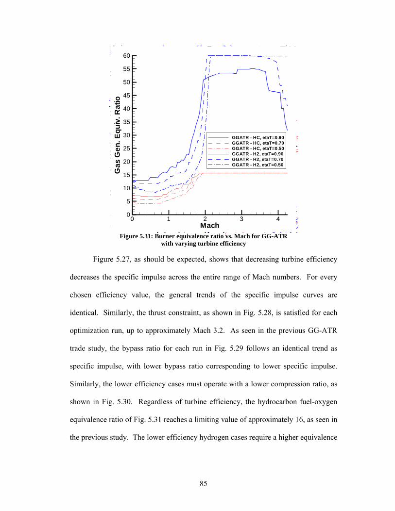
Mach
yp
0 1 2 3 40
5
10
15
20
25
30
35
40
45
50
55
60
GGATR - HC, etaT=0.90GGATR - HC, etaT=0.70GGATR - HC, etaT=0.50GGATR - H2, etaT=0.90GGATR - H2, etaT=0.70GGATR - H2, etaT=0.50
Spe
cific
Impu
lse
400
600
800
1000
1200
1400
1600
1800
2000
GGATR - HC, T_fuel=200KGGATR - HC, T_fuel=300KGGATR - HC, T_fuel=400KGGATR - HC, T_fuel=500KGGATR - HC, T_fuel=1000K
Byp
ass
Rat
io
4
6
8
10
12
14
16
18
20
GGATR - HC, T_fuel=200KGGATR - HC, T_fuel=300KGGATR - HC, T_fuel=400KGGATR - HC, T_fuel=500Kas
Gen
.Equ
iv.R
atio
20
30
40
50
se 4000
5000
6000
40
50
60
Mach1 2 3 4
GGATR - HC, Phi=opt.GGATR - HC, Phi=10GGATR - HC, Phi=6GGATR - H2, Phi=opt.GGATR - H2, Phi=10GGATR - H2, Phi=6
Mach1 2 3 4
GGATR - H2, Phi=6
Mach1 2 3 4
GGATR - HC, Phi=opt.GGATR - HC, Phi=10GGATR - HC, Phi=6GGATR - H2, Phi=opt.GGATR - H2, Phi=10GGATR - H2, Phi=6
Thru
st
00
1
2
Com
pres
sorP
ress
ure
R
00
0.5
1
1.5
2
2.5
3
3.5
Mach0 1 2 3 4
0
0
0
0
GGATR - HC, etaT=0.90GGATR - HC, etaT=0.70GGATR - HC, etaT=0.50GGATR - H2, etaT=0.90GGATR - H2, etaT=0.70GGATR - H2, etaT=0.50
Mach
Gas
Gen
.Equ
iv.R
atio
0 1 2 3 40
5
10
15
20
25
30
35
40
45
50
55
60
GGATR - HC, etaT=0.90GGATR - HC, etaT=0.70GGATR - HC, etaT=0.50GGATR - H2, etaT=0.90GGATR - H2, etaT=0.70GGATR - H2, etaT=0.50
Figure 5.31: Burner equivalence ratio vs. Mach for GG-ATR
with varying turbine efficiency
Figure 5.27, as should be expected, shows that decreasing turbine efficiency
decreases the specific impulse across the entire range of Mach numbers. For every
chosen efficiency value, the general trends of the specific impulse curves are
identical. Similarly, the thrust constraint, as shown in Fig. 5.28, is satisfied for each
optimization run, up to approximately Mach 3.2. As seen in the previous GG-ATR
trade study, the bypass ratio for each run in Fig. 5.29 follows an identical trend as
specific impulse, with lower bypass ratio corresponding to lower specific impulse.
Similarly, the lower efficiency cases must operate with a lower compression ratio, as
shown in Fig. 5.30. Regardless of turbine efficiency, the hydrocarbon fuel-oxygen
equivalence ratio of Fig. 5.31 reaches a limiting value of approximately 16, as seen in
the previous study. The lower efficiency hydrogen cases require a higher equivalence
85

ratio, and actually reach the user-imposed design variable limit of 60 at about Mach
2.0.
Changes in efficiency have a greater impact at lower Mach numbers, where,
as indicated in Fig. 5.30, the compressor operates at a higher pressure ratio. At Mach
1.0, the difference in efficiency of the 90% and 70% hydrogen-fueled runs is about
300 sec., or approximately 10%. The difference between the 90% and 50% hydrogen
runs is approximately 20%. By Mach 2.5, these differences decrease to about 1.5%
and 3% for the 70% and 50% efficiency cases, respectively. Similar results are seen
for the hydrocarbon-fuel cases, as well. Thus, despite a turbine efficiency penalty by
as much 40%, the GG-ATR appears to maintain operability.
5.3.3 Reactant Inlet Temperature
The reactant inlet temperature is very important in the GG-ATR analysis. For
the TBE, a small amount of fuel combines with a large quantity of air before
combustion, so the fuel temperature has relatively little effect on the bulk flow
properties. In the gas generator, however, only stored fuel and oxygen are
combusted, so the assumed inlet temperature should have a greater impact. To
determine the importance of the reactant inlet temperature, the same trade study
performed on the TBE is performed here, optimizing with fuel and oxygen inlet
temperature values of 300K, 400K, 500K, and 1000K, in addition to the baseline of
200K. All other parameters assume the baseline values given as runs “GGATR1” and
“GGATR2,” in Table 5.4.
Figures 5.32 and 5.33 illustrate the variation of specific impulse with
propellant inlet temperature for hydrocarbon and hydrogen fuel, respectively. The
86

normalized thrust and design variable values follow the same trends seen in the
previous two studies and, as such, are not given. Both figures demonstrate that
increased propellant inlet temperatures results in higher specific impulse across the
entire flight range. For hydrocarbon fuel, an increase in fuel inlet temperature
provides the same increase in specific impulse at any Mach number. Each increment
of 100K increases the specific impulse by approximately 1.5%. Increases in
propellant temperature for the hydrogen-fueled GG-ATR, however, provide greater
benefits at lower Mach numbers. As shown in Fig. 5.33, a 1000K inlet temperature
provides 50% greater impulse than a 200K inlet temperature at Mach 1.0. By Mach
3.0, this benefit is only about 25%. Regardless of Mach number, the hydrogen-fueled
GG-ATR benefits more from increases in fuel temperature than the hydrocarbon.
Byp
ass
Rat
io
0 1 2 3 40
2
4
6
8
10
12
14
16
18
20
GGATR - HC, T_fuel=200KGGATR - HC, T_fuel=300KGGATR - HC, T_fuel=400KGGATR - HC, T_fuel=500KGGATR - HC, T_fuel=1000KG
asG
en.E
quiv
.Rat
io
10
20
30
40
50
GGATR - HC, T_fuel=20GGATR - HC, T_fuel=30GGATR - HC, T_fuel=40GGATR - HC, T_fuel=50GGATR - HC, T_fuel=10
ecifi
cIm
puls
e
3000
4000
5000
6000
ssR
atio 30
40
50
uiv.
Rat
io
40
60
Mach2 3 4
GGATR - HC, Phi=opt.GGATR - HC, Phi=10GGATR - HC, Phi=6GGATR - H2, Phi=opt.GGATR - H2, Phi=10GGATR - H2, Phi=6
Mach2 3 4
Mach2 3 4
GGATR - HC, Phi=opt.GGATR - HC, Phi=10GGATR - HC, Phi=6GGATR - H2, Phi=opt.GGATR - H2, Phi=10GGATR - H2, Phi=6
00
1
Com
pres
so
00
0.5
1
1.5
2
CP
RTh
rust
Mach0 1 2 3 4
GGATR - HC, etaT=0.90GGATR - HC, etaT=0.70GGATR - HC, etaT=0.50GGATR - H2, etaT=0.90GGATR - H2, etaT=0.70GGATR - H2, etaT=0.50
Mach1 2 3 4
GGATR - H2, etaT=0.70GGATR - H2, etaT=0.50
Mach1 2 3 4
GGATR - HC, etaT=0.90GGATR - HC, etaT=0.70GGATR - HC, etaT=0.50GGATR - H2, etaT=0.90GGATR - H2, etaT=0.70GGATR - H2, etaT=0.50
Mach
Spe
cific
Impu
lse
0 1 2 3 40
200
400
600
800
1000
1200
1400
1600
1800
2000
GGATR - HC, T_fuel=200KGGATR - HC, T_fuel=300KGGATR - HC, T_fuel=400KGGATR - HC, T_fuel=500KGGATR - HC, T_fuel=1000K
Figure 5.32: Specific impulse vs. Mach for GG-ATR
with varying hydrocarbon fuel inlet temperature
87

h3 4 C
o
00
0.5
1
0 10
Mach2 3 4
,
Mach2 3 4Mach
2 3 4
GGATR HC, etaT 0.50GGATR - H2, etaT=0.90GGATR - H2, etaT=0.70GGATR - H2, etaT=0.50
Mach1 2 3 4
GGATR - HC, T_fuel=200KGGATR - HC, T_fuel=300KGGATR - HC, T_fuel=400KGGATR - HC, T_fuel=500KGGATR - HC, T_fuel=1000K
Thru
s
0
1
2
Com
pres
sorP
ress
u
Mach1 2 3 4
GGATR - HC, T_fuel=200KGGATR - HC, T_fuel=300KGGATR - HC, T_fuel=400KGGATR - HC, T_fuel=500KGGATR - HC, T_fuel=1000K
Mach0 1 2 3 4
GGATR - HC, T_fuel=200KGGATR - HC, T_fuel=300KGGATR - HC, T_fuel=400KGGATR - HC, T_fuel=500KGGATR - HC, T_fuel=1000K
Gas
Gen
.Equ
iv.R
atio
20
40
60
GGATR - H2, T_fuel=200KGGATR - H2, T_fuel=300KGGATR - H2, T_fuel=400KGGATR - H2, T_fuel=500KGGATR - H2, T_fuel=1000K
Byp
ass
Rat
io
0 1 2 3 40
10
20
30
40
50
GGATR - H2, T_fuel=200KGGATR - H2, T_fuel=300KGGATR - H2, T_fuel=400KGGATR - H2, T_fuel=500KGGATR - H2, T_fuel=1000K
Mach
Spe
cific
Impu
lse
0 1 2 3 40
1000
2000
3000
4000
5000
6000
GGATR - H2, T_fuel=200KGGATR - H2, T_fuel=300KGGATR - H2, T_fuel=400KGGATR - H2, T_fuel=500KGGATR - H2, T_fuel=1000K
Figure 5.33: Specific impulse vs. Mach for GG-ATR
with varying hydrogen fuel inlet temperature
5.4 EX-ATR Trade Studies
The EX-ATR is actually the simplest TBCC engine, computationally,
requiring only two design variables to define its performance. As the afterburner
fuel-air ratio (not equivalence ratio) is simply the inverse of bypass ratio, the only
required EX-ATR design variables are the compressor pressure ratio and bypass ratio.
The fuel inlet temperature and turbine performance, however, become exceedingly
important in the EX-ATR, because the turbine inlet flow is heated through active
cooling, alone. The fuel inlet temperature will actually be limited by the heat
exchanger and engine cooling technology, and such, could vary significantly. In
addition to fuel inlet temperature, the fuel inlet pressure (P4) and turbine efficiency
88

are also directly related to the turbine performance, and as such, all three parameters
will be subjects of EX-ATR performance trade studies.
5.4.1 Fuel Inlet Temperature
While relatively low reactant temperatures are assumed in the TBE and GG-
ATR, the EX-ATR requires, by definition, this temperature to be quite high for the
engine to operate. With no core combustor, the engine relies solely on the expansion
of heated, pressurized fuel to drive the turbine. This temperature increase is most
likely to be supplied through active cooling, so it is actually the cooling system’s heat
exchanger technology that limits the fuel inlet temperature. The baseline EX-ATR
case assumes an inlet temperature of 1000K, but cases are also optimized with fuel
inlet temperatures of 900K and 800K. Both hydrogen and hydrocarbon fuels are
used, with the corresponding design variable values given in Table 5.5.
Table 5.5: EX-ATR fuel temperature trade study input parameters Run min
M max M ∆M min
πc
max πc
min α
max α fuel T4
EXATR1 0 4.26 0.05 1 10 1 30 HC 1000K
EXATR2 0 4.26 0.05 1 10 1 60 H2 1000K
EXATR3 0 4.26 0.05 1 10 1 30 HC 900K
EXATR4 0 4.26 0.05 1 10 1 60 H2 900K
EXATR5 0 4.26 0.05 1 10 1 30 HC 800K
EXATR6 0 4.26 0.05 1 10 1 60 H2 800K
Figures 5.34-5.37 demonstrate how specific impulse, thrust, and the design
variables vary with fuel inlet temperature. The hydrogen-fueled cases of Fig. 5.34
show a similar trend in specific impulse to that demonstrated by the GG-ATR. As in
all other engines, specific impulse decreases from Mach 0.0 to Mach 1.0, and then
increases up to a knee in the curve at about Mach 2.5. Comparing the hydrogen and
hydrocarbon cases in Fig. 5.34, it is immediately apparent that decreased fuel
89

temperatures impact the hydrocarbon-fueled EX-ATR more severely. A decrease in
hydrogen fuel temperature of 100K decreases the specific impulse by approximately
200 sec., or about 5%. A 100K decrease in hydrocarbon inlet temperature, however,
reduces specific impulse from 1800 sec. at Mach 2, to 400 sec.; almost an 80% drop
in performance. Additionally, as shown in Fig. 5.35, from Mach 0.4 to 1.0, the no
EX-ATR case is able to maintain the minimum thrust constraint. As seen in the GG-
ATR results, the bypass ratio curves of Fig. 5.36 follow the trends of specific impulse
exactly. Figure 5.37 indicates that the lower bypass ratios of the 800K and 900K
hydrocarbon cases allow the engine to operate at a higher compression ratio, as
relatively less air is passing through the compressor. As demonstrated in the GG-
ATR, the compressor operates with a maximum compression ratio of about 3.5 for
the cases providing reasonable specific impulse.
EXATR - HC, T4=1000KEXATR - HC, T4=900KEXATR - HC, T4=800KEXATR - H2, T4=1000KEXATR - H2, T4=900KEXATR - H2, T4=800K
Spe
cific
Impu
lse
(sec
)
2000
3000
4000
5000
EXATR - HCEXATR - HCEXATR - HCEXATR - H2EXATR - H2EXATR - H2
Byp
ass
Rat
io
20
30
40
50
EXATREXATREXATREXATREXATREXATR
6000Mach
Spe
cific
Impu
lse
(sec
)
0 1 2 3 40
1000
2000
3000
4000
5000
EXATR - HC, T4=1000KEXATR - HC, T4=900KEXATR - HC, T4=800KEXATR - H2, T4=1000KEXATR - H2, T4=900KEXATR - H2, T4=800K
Figure 5.34: Specific impulse vs. Mach for EX-ATR
with varying fuel inlet temperature
90

0.900.700.500.900.700.50
Com
pres
ison
Rat
io
0 1 2 3 41
1.5
2
2.5
3
3.5
4
4.5
5
5.5
EXATR - HC, T4=1000KEXATR - HC, T4=900KEXATR - HC, T4=800KEXATR - H2, T4=1000KEXATR - H2, T4=900KEXATR - H2, T4=800K
Nor
mal
ized
Thru
st
2
3
4
5
EXATR -EXATR -EXATR -EXATR -EXATR4
4
mpr
esis
onR
atio
2
3
4
5
EXEXEXEXEXEX
Mach
Nor
mal
ized
Thru
st
0 1 2 3 40
1
2
3
4
EXATR - HC, T4=1000KEXATR - HC, T4=900KEXATR - HC, T4=800KEXATR - H2, T4=1000KEXATR - H2, T4=900KEXATR - H2, T4=800K
Tmin
Figure 5.35: Thrust vs. Mach for EX-ATR
with varying fuel inlet temperature
Spe
cific
Impu
lse
(sec
)
2000
3000
4000
5000
EXATR - HC, etaEXATR - HC, etaEXATR - HC, etaEXATR - H2, etaEXATR - H2, etaEXATR - H2, eta
Byp
ass
Rat
io
20
30
40
50
EXATR - HCEXATR - HCEXATR - HCEXATR - H2EXATR - H2EXATR - H2
5000
6000Mach
pp
()
0 1 2 3 40
1000
2000
3000
4000
5000
EXATR - HC, T4=1000KEXATR - HC, T4=900KEXATR - HC, T4=800KEXATR - H2, T4=1000KEXATR - H2, T4=900KEXATR - H2, T4=800K
Mach
Byp
ass
Rat
io
0 1 2 3 40
10
20
30
40
50
EXATR - HC, T4=1000KEXATR - HC, T4=900KEXATR - HC, T4=800KEXATR - H2, T4=1000KEXATR - H2, T4=900KEXATR - H2, T4=800K
Figure 5.36: Bypass ratio vs. Mach for EX-ATR
with varying fuel inlet temperature
91

Nor
mal
ized
Thru
st
2
3
4
5
EXATR - HC,EXATR - HC,EXATR - HC,EXATR - H2,EXATR - H2,EXATR - H2,
4
4
Com
pres
ison
Rat
io
2
3
4
5
EXATREXATREXATREXATREXATREXATR
Mach0 1 2 3 4
0
1
2
3
EXATR - HC, T4=1000KEXATR - HC, T4=900KEXATR - HC, T4=800KEXATR - H2, T4=1000KEXATR - H2, T4=900KEXATR - H2, T4=800K
Mach
Com
pres
ison
Rat
io
0 1 2 3 41
1.5
2
2.5
3
3.5
4
4.5
5
5.5
EXATR - HC, T4=1000KEXATR - HC, T4=900KEXATR - HC, T4=800KEXATR - H2, T4=1000KEXATR - H2, T4=900KEXATR - H2, T4=800K
Figure 5.37: Compressor ratio vs. Mach for EX-ATR
with varying fuel inlet temperature
5.4.2 Turbine Efficiency
An identical turbine efficiency trade study to that of the GG-ATR is also
performed for the EX-ATR. The turbines of the two ATR engines should operate
similarly, but the lack of oxygen and lower operating temperature may change the
relative impact of turbine efficiency on EX-ATR performance. All optimization runs
in this study assume the baseline input values from runs “EXATR1” and “EXATR2,”
above, and are optimized for turbine efficiencies of 50% and 70% in addition to the
baseline 90% value.
Figures 5.38-5.41 show the specific impulse, thrust, bypass ratio, and
compressor pressure ratio, respectively, for this trade study. From Fig. 5.38, it is seen
that a 20% decrease in turbine efficiency does impact specific impulse slightly, but a
92

40% decrease, regardless of fuel type, severely degrades EX-ATR performance. At
Mach 2.0, the difference in specific impulse from 90% to 70% efficiency is
approximately 5% of the baseline value; the difference between 90% and 50%
efficiency jumps to almost 50% of the baseline for hydrogen fuel and 80% for
hydrocarbon. Figure 5.39 shows that the 50% efficiency hydrogen case, while
feasible, cannot even follow the minimum thrust constraint in the same manner as all
other cases. Figures 5.40 and 5.41 demonstrate the same trends seen in the EX-ATR
fuel temperature study: bypass ratio follows an identical trend to specific impulse,
and the poor performing hydrocarbon-fueled case operates at a slightly higher
compressor pressure ratio than the other cases. Once again, the maximum pressure
ratio of the non-degraded cases is about 3.5.
puls
e(s
ec)
4000
5000
6000
EXATR - HC, P4=2000 kPaEXATR - HC, P4=3000 kPaEXATR - HC, P4=4000 kPaEXATR - H2, P4=2000 kPatio
40
50
EXATR - HC, P4=2
Mach1 2 3 4
EXATR - HC, T4=1000KEXATR - HC, T4=900KEXATR - HC, T4=800KEXATR - H2, T4=1000KEXATR - H2, T4=900KEXATR - H2, T4=800K
Mach1 2 3 4
EXATR - HC, T4=1000KEXATR - HC, T4=900KEXATR - HC, T4=800KEXATR - H2, T4=1000KEXATR - H2, T4=900KEXATR - H2, T4=800K
Nor
mal
ized
Thru
0
1
2
Com
pres
ison
Rat
io
Byp
ass
Rat
io
0 1 2 3 40
10
20
30
40
50
EXATR - HC, etaT=0.90EXATR - HC, etaT=0.70EXATR - HC, etaT=0.50EXATR - H2, etaT=0.90EXATR - H2, etaT=0.70EXATR - H2, etaT=0.50
Mach
Spe
cific
Impu
lse
(sec
)
0 1 2 3 40
1000
2000
3000
4000
5000
EXATR - HC, etaT=0.90EXATR - HC, etaT=0.70EXATR - HC, etaT=0.50EXATR - H2, etaT=0.90EXATR - H2, etaT=0.70EXATR - H2, etaT=0.50
Figure 5.38: Specific impulse vs. Mach for EX-ATR
with varying turbine efficiency
93

Rat
io
2.5
3
3.5
4
EXATR - HC, P4=2000EXATR - HC, P4=3000EXATR - HC, P4=4000EXATR - H2, P4=2000EXATR - H2, P4=3000EXATR - H2, P4=4000
edTh
rust
3
4
EXATR - HC, P4=2000 kPaEXATR - HC, P4=3000 kPaEXATR - HC, P4=4000 kPaEXATR - H2, P4=2000 kPa
Mach2 3 4
EXATR - HC, T4=1000KEXATR - HC, T4=900KEXATR - HC, T4=800KEXATR - H2, T4=1000KEXATR - H2, T4=900KEXATR - H2, T4=800K
Mach1 2 3 4
EXATR - H2, T4=800K
Com
pres
ison
Rat
io
0 1 2 3 40
1
2
3
4
5
EXATR - HC, etaT=0.90EXATR - HC, etaT=0.70EXATR - HC, etaT=0.50EXATR - H2, etaT=0.90EXATR - H2, etaT=0.70EXATR - H2, etaT=0.50
Mach
Nor
mal
ized
Thru
st
0 1 2 3 40
1
2
3
4
5
EXATR - HC, etaT=0.90EXATR - HC, etaT=0.70EXATR - HC, etaT=0.50EXATR - H2, etaT=0.90EXATR - H2, etaT=0.70EXATR - H2, etaT=0.50
Tmin
Figure 5.39: Thrust vs. Mach for EX-ATR with varying turbine efficiency
Mach0 1 2 3 4
0
1000
2000
3000
EXATR - HC, etaT=0.90EXATR - HC, etaT=0.70EXATR - HC, etaT=0.50EXATR - H2, etaT=0.90EXATR - H2, etaT=0.70EXATR - H2, etaT=0.50
mpu
lse
(sec
)
3000
4000
5000
6000
EXATR - HC, P4=2000 kPaEXATR - HC, P4=3000 kPaEXATR - HC, P4=4000 kPaEXATR - H2, P4=2000 kPaEXATR - H2, P4=3000 kPaEXATR - H2, P4=4000 kPaR
atio
30
40
50
EXATR - HC, P4=2000 kEXATR - HC, P4=3000 kEXATR - HC, P4=4000 k
Mach1 2 3 4
,EXATR - HC, T4=800KEXATR - H2, T4=1000KEXATR - H2, T4=900KEXATR - H2, T4=800K
Mach1 2 3 4
EXATR - HC, T4=1000KEXATR - HC, T4=900KEXATR - HC, T4=800KEXATR - H2, T4=1000KEXATR - H2, T4=900KEXATR - H2, T4=800K
Nor
mal
ized
Th
00
1
2
Com
pres
ison
Rat
1
1.5
2
2.5
3
3.5
4
Mach
Byp
ass
Rat
io
0 1 2 3 40
10
20
30
40
50
EXATR - HC, etaT=0.90EXATR - HC, etaT=0.70EXATR - HC, etaT=0.50EXATR - H2, etaT=0.90EXATR - H2, etaT=0.70EXATR - H2, etaT=0.50
Figure 5.40: Bypass ratio vs. Mach for EX-ATR
with varying turbine efficiency
94

Mach
Nor
mal
ized
Thru
st
0 1 2 3 40
1
2
3
4
EXATR - HC, etaT=0.90EXATR - HC, etaT=0.70EXATR - HC, etaT=0.50EXATR - H2, etaT=0.90EXATR - H2, etaT=0.70EXATR - H2, etaT=0.50
son
Rat
io
2.5
3
3.5
4
EXATR - HC, P4=2000 kPEXATR - HC, P4=3000 kPEXATR - HC, P4=4000 kPEXATR - H2, P4=2000 kPEXATR - H2, P4=3000 kPEXATR - H2, P4=4000 kP
aliz
edTh
rust
2
3
4
EXATR - HC, P4=2000 kPaEXATR - HC, P4=3000 kPaEXATR - HC, P4=4000 kPaEXATR - H2, P4=2000 kPaEXATR - H2, P4=3000 kPaEXATR - H2, P4=4000 kPa
Mach2 3 4
,EXATR - HC, T4=800KEXATR - H2, T4=1000KEXATR - H2, T4=900KEXATR - H2, T4=800K
Mach1 2 3 4
Mach
Com
pres
ison
Rat
io
0 1 2 3 40
1
2
3
4
5
EXATR - HC, etaT=0.90EXATR - HC, etaT=0.70EXATR - HC, etaT=0.50EXATR - H2, etaT=0.90EXATR - H2, etaT=0.70EXATR - H2, etaT=0.50
Figure 5.41: Compressor ratio vs. Mach for EX-ATR
with varying turbine efficiency
5.4.3 Chamber pressure
A final trade study investigates the in the impact of the expander section inlet
pressure (P4) on EX-ATR performance. The baseline case assumes an injection
pressure of 2000 kPa, or approximately 20 atm. This is one-half of the value assumed
for GG-ATR chamber pressure. This value is chosen because the lack of combustion
may make it difficult to maintain a high pressure in the EX-ATR. However, to verify
the effects of increasing this pressure, additional EX-ATR cases with chamber
pressures of 3000 kPa and 4000 kPa are optimized. These cases assume 90% turbine
efficiency and use the baseline input parameters, given as runs “EXATR1” and
“EXATR2,” in Table 5.5.
95

The results of this study are given in Figs. 5.42-5.45. Figure 5.42 shows that
increasing the chamber pressure increases the specific impulse slightly for the
hydrogen-fueled EX-ATR, but has almost no effect whatsoever on hydrocarbon-
fueled performance. Higher chamber pressures have a larger impact on specific
impulse at lower speeds. At Mach 1.5, the hydrogen-fueled specific impulse
increases by 10% and 15% for 3000 kPa and 4000 kPa pressures, respectively. At
Mach 3.0, however, the impact is less than half as severe. Figure 5.44 shows a
similar thrust response to the previous EX-ATR cases: all optimization runs slightly
violate the minimum thrust constraint from about Mach 0.4 to 1.0, and then cannot
satisfy it at all above Mach 3.4. Once again, bypass ratio, as seen in Fig. 5.44,
follows the specific impulse trends exactly, while all runs produce compression ratios
of approximately 3.5 at Mach 0.5, decreasing to almost 1.0 by Mach 4.0.
Byp
ass
Rat
io
0 1 2 3 40
10
20
30
40
50
EXATR - HC, P4=2000 kPaEXATR - HC, P4=3000 kPaEXATR - HC, P4=4000 kPaEXATR - H2, P4=2000 kPaEXATR - H2, P4=3000 kPaEXATR - H2, P4=4000 kPa
Mach2 3 4
Mach2 3 4
00
01
1.5
Mach0 1 2 3 4
0
0
0
Mach1 2 3 4
Mach
Spe
cific
Impu
lse
(sec
)
0 1 2 3 40
1000
2000
3000
4000
5000
6000
EXATR - HC, P4=2000 kPaEXATR - HC, P4=3000 kPaEXATR - HC, P4=4000 kPaEXATR - H2, P4=2000 kPaEXATR - H2, P4=3000 kPaEXATR - H2, P4=4000 kPa
Figure 5.42: Specific impulse vs. Mach for EX-ATR
with varying chamber pressure
96

Com
pres
ison
Rat
io
0 1 2 3 40
0.5
1
1.5
2
2.5
3
3.5
4
EXATR - HC, P4=2000 kPaEXATR - HC, P4=3000 kPaEXATR - HC, P4=4000 kPaEXATR - H2, P4=2000 kPaEXATR - H2, P4=3000 kPaEXATR - H2, P4=4000 kPa
Mach2 3 4
Mach2 3 4
Mach
p
0 1 2 3 40
1
2
Mach0 1 2 3 4
0
1
2,
EXATR - HC, etaT=0.70EXATR - HC, etaT=0.50EXATR - H2, etaT=0.90EXATR - H2, etaT=0.70EXATR - H2, etaT=0.50
Mach
Nor
mal
ized
Thru
st
0 1 2 3 40
1
2
3
4
EXATR - HC, P4=2000 kPaEXATR - HC, P4=3000 kPaEXATR - HC, P4=4000 kPaEXATR - H2, P4=2000 kPaEXATR - H2, P4=3000 kPaEXATR - H2, P4=4000 kPa
Figure 5.43: Thrust vs. Mach for EX-ATR
with varying chamber pressure
MachMach2 3 4 0
1
Mach1 2 3 4Mach
1 2 3 4
Mach0 1 2 3 4
0
1000
2000
3000
4000
5000
EXATR - HC, P4=2000 kPaEXATR - HC, P4=3000 kPaEXATR - HC, P4=4000 kPaEXATR - H2, P4=2000 kPaEXATR - H2, P4=3000 kPaEXATR - H2, P4=4000 kPa
Mach
Byp
ass
Rat
io
0 1 2 3 40
10
20
30
40
50
EXATR - HC, P4=2000 kPaEXATR - HC, P4=3000 kPaEXATR - HC, P4=4000 kPaEXATR - H2, P4=2000 kPaEXATR - H2, P4=3000 kPaEXATR - H2, P4=4000 kPa
Tmin
Figure 5.44: Bypass ratio vs. Mach for EX-ATR with varying chamber pressure
97

MachMach2 3 4
Mach0 1 2 3 4
Mach1 2 3 4
EXATR - H2, etaT=0.90EXATR - H2, etaT=0.70EXATR - H2, etaT=0.50
Mach0 1 2 3 4
0
1
2
3
EXATR - HC, P4=2000 kPaEXATR - HC, P4=3000 kPaEXATR - HC, P4=4000 kPaEXATR - H2, P4=2000 kPaEXATR - H2, P4=3000 kPaEXATR - H2, P4=4000 kPa
Mach
Com
pres
ison
Rat
io
0 1 2 3 40
0.5
1
1.5
2
2.5
3
3.5
4
EXATR - HC, P4=2000 kPaEXATR - HC, P4=3000 kPaEXATR - HC, P4=4000 kPaEXATR - H2, P4=2000 kPaEXATR - H2, P4=3000 kPaEXATR - H2, P4=4000 kPa
Figure 5.45: Compressor ratio vs. Mach for EX-ATR
with varying chamber pressure
5.5 Engine Comparison
Now that each TBCC engine has been analyzed individually, they may all be
compared in order to determine the most suitable propulsion system for the first stage
of a TSTO RLV. Pure turbojet and pure ramjet engine performance is also included
as a reference. For the combined-cycle engines to be effective, they should at least
outperform the reference single-cycle engines. The RJ and TJ optimization is
substantially less complicated than the other engines, as the RJ only requires a fuel-air
equivalence ratio to be specified, and the TJ requires only an equivalence ratio and
compressor pressure ratio. The RJ optimization results are given up to Mach 5.0, as it
is not limited by the compressor temperature constraint of the other engines. The RJ
and TJ optimization runs assume 200K fuel inlet temperature and compressor and
98

turbine efficiencies of 88% and 90%, respectively. The baseline engine parameters
for the TBCC engines are used for this comparison. The exact design variable input
values for each engine optimization run are given in Table 5.6, below. The engines
are optimized and compared for both hydrogen and hydrocarbon fuel, and for the sake
of simplicity, these results will be presented separately.
Table 5.6: TBCC engine comparison input parameters Run min
M max M ∆M min
πc
max πc
min ΦB
max ΦB
min α
max α
min ΦAB
max ΦAB
fuel
RJ1 0 5.0 0.05 - - 0.001 1 - - - - HC
RJ2 0 5.0 0.05 - - 0.001 1 - - - - H2
TJ1 0 4.26 0.05 1 40 0.001 1 - - - - HC
TJ2 0 4.26 0.05 1 40 0.001 1 - - - - H2
TBE1 0 4.26 0.05 1 40 0.001 1 0.001 0.95 0.001 1 HC
TBE2 0 4.26 0.05 1 40 0.001 1 0.001 0.95 0.001 1 H2
GGATR1 0 4.26 0.05 1 10 1 30 1 30 - - HC
GGATR2 0 4.26 0.05 1 10 1 60 1 60 - - H2
EXATR1 0 4.26 0.05 1 10 - - 1 30 - - HC
EXATR2 0 4.26 0.05 1 10 - - 1 60 - - H2
5.5.1 Hydrocarbon-Fueled TBCC Comparison
Figures 5.46-5.48 present specific impulse, normalized thrust, and compressor
pressure ratio curves for all five engines. A ramjet case is obviously not present in
the compression ratio curve, and no other design variables are plotted, as compression
ratio is the only variable that can be compared directly for every TBCC engine.
Figure 5.46 shows that the TBE provides the highest specific impulse of any
hydrocarbon-fueled engine, up to Mach 3.5. Above Mach 3.5, as shown in Fig. 5.47,
the minimum thrust constraint cannot be satisfied for all engines, so a direct
comparison is difficult. The pure TJ and RJ engines are unable to satisfy the
minimum thrust constraint for the majority of the flight range. The RJ cannot provide
sufficient thrust for speeds lower than Mach 2.5, while the TJ cannot produce
99

sufficient thrust for speeds higher than Mach 2.5. As such, this point represents the
speed at which the “low-speed correction” of turbomachinery is no longer required
and the RJ becomes superior to the TJ. This result is not reflected in the specific
impulse curves of Fig. 5.46, however, as all TJ performance above Mach 2.5 is
calculated with a violated thrust constraint. As seen in the previous trade studies, the
hydrocarbon-fueled ATR cannot satisfy the minimum thrust constraint from Mach
0.4-1.0, and its specific impulse performance is also poor across this range.
As intended, the TBE provides specific impulse performance greater than that
of the TJ and RJ engines upon which it is based. It is also able to satisfy the
minimum thrust constraint for all Mach numbers up to approximately Mach 3.5. The
TBE and TJ produce specific impulse on the order of 4000 sec. at takeoff, while the
GG-ATR and EX-ATR produce values of 1300 sec. and 1700 sec., respectively. By
approximately Mach 2.5, at the knee in every specific impulse curve, RJ specific
impulse is actually greater than GG-ATR, but the EX-ATR specific impulse is within
about 3% of the TJ. As Mach number increases, performance of each engine
converges towards that of the RJ. Returning to the definition of a turbojet in Chap. 2,
this makes sense, as the turbomachinery of each TBCC engine essentially acts as a
low-speed correction to a ramjet. Thus, at high speeds, this turbomachinery becomes
less necessary, and all TBCC engines tend to operate in a more ramjet-like mode.
This result is also verified in Fig. 5.48, which shows that, as Mach number increases,
the compression ratio of every engine approaches 1.0. This figure also shows that the
TBE and TJ engines operate at ten times the compression ratio of the ATR engines at
low speed.
100

Nor
mal
ized
Thru
st
0
1
2
3
4
TJ - HCRJ - HCTBE - HCGGATR - HCEXATR - HC
Com
pres
orP
ress
ure
Rat
io
10
20
30
40
TJ - HCTBE - HCGGATR -EXATR -
Mach
Spe
cific
Impu
lse
(sec
)
0 1 2 3 4 50
1000
2000
3000
4000
5000
TJ - HCRJ - HCTBE - HCGGATR - HCEXATR - HC
Figure 5.46: Specific impulse comparison for TJ, RJ,
and TBCC engines burning hydrocarbon fuel
Com
pres
orP
ress
ure
Rat
io
0 1 2 3 40
10
20
30
40
TJ - HCTBE - HCGGATR - HCEXATR - HC
Mach0 1 2 3 4 5
0
1000
2000
3000
4000TJ - HCRJ - HCTBE - HCGGATR - HCEXATR - HC
Mach
Nor
mal
ized
Thru
st
0 1 2 3 4 50
1
2
3
4
TJ - HCRJ - HCTBE - HCGGATR - HCEXATR - HC
Tmin
Figure 5.47: Thrust comparison for TJ, RJ,
and TBCC engines burning hydrocarbon fuel
101

Mach0 1 2 3 4 5
TJ - HCRJ - HCTBE - HCGGATR - HCEXATR - HC
Mach0 1 2 3 4 5
0
1
2
3
TJ - HCRJ - HCTBE - HCGGATR - HCEXATR - HC
Mach
Com
pres
orP
ress
ure
Rat
io
0 1 2 3 4 50
10
20
30
40
TJ - HCTBE - HCGGATR - HCEXATR - HC
Figure 5.48: Compressor ratio comparison for TJ, RJ, and TBCC engines burning hydrocarbon fuel
5.5.2 Hydrogen-Fueled TBCC Comparison
The hydrogen-fueled engines demonstrate similar trends to the hydrocarbon
results. As seen in the previous studies, hydrogen fuel produces significantly higher
specific impulse for every engine across the entire range of Mach numbers. A
comparison between Figs. 5.49 and 5.46 shows that hydrogen-fueled TJ, TBE, GG-
ATR, and EX-ATR produce almost three times the specific impulse of their
hydrocarbon-fueled counterparts at takeoff. Another major difference in Fig. 5.49 is
that EX-ATR performance is substantially greater than that of the GG-ATR. This is
especially apparent below Mach 2.0, where the EX-ATR performance is superior by
approximately 2000 sec.
102

Most of the other trends of Fig. 5.49 are the same as those seen for
hydrocarbon fuel. The TBE provides the best specific impulse performance up to
about Mach 3.0. A comparison is limited above this point because the minimum
thrust constraint is violated by the TJ above about Mach 2.5, and violated by the other
engines past Mach 3.4. This point is illustrated in the thrust curves of Fig. 5.50. TBE
and TJ specific impulse drops off drastically from Mach 0.0 to Mach 2.5, but the
ATR engines maintain relatively even performance at any speed. The GG-ATR
maintains a specific impulse between 3000 and 4000 sec., and the EX-ATR between
4000 and 5000 sec. across the entire flight range. All curves, as seen before, have a
knee in them at approximately Mach 2.5, and this speed also represents the point in
the flight regime where hydrogen-fueled RJ operation is more beneficial than TJ.
Finally, Fig. 5.51 shows almost identical compressor pressure ratios for hydrogen fuel
as seen in hydrocarbon, with the ATR engines operating at an order-of-magnitude
lower compression ratios below Mach 1.0.
103

Com
pres
orP
ress
ure
Rat
io
10
20
30
40
TJ - H2TBE - H2GGATR - H2EXATR - H2
M h
Nor
mal
ized
Thru
st
0 1 2 3 40
1
2
3
4
TJ - H2RJ - H2TBE - H2GGATR - H2EXATR - H2
Mach
Spe
cific
Impu
lse
(sec
)
0 1 2 3 4 50
2000
4000
6000
8000
10000
12000
TJ - H2RJ - H2TBE - H2GGATR - H2EXATR - H2
Figure 5.49: Specific impulse comparison for TJ, RJ,
and TBCC engines burning hydrogen fuel
Mach0 1 2 3 4 5
0
2000
4000
6000
8000
0000
2000
TJ - H2RJ - H2TBE - H2GGATR - H2EXATR - H2
Com
pres
orP
ress
ure
Rat
io
0
10
20
30
40
TJ - H2TBE - H2GGATR - H2EXATR - H2
Mach
Nor
mal
ized
Thru
st
0 1 2 3 4 50
1
2
3
4
TJ - H2RJ - H2TBE - H2GGATR - H2EXATR - H2
Tmin
Figure 5.50: Thrust comparison for TJ, RJ, and TBCC engines burning hydrogen fuel
104

Mach0 1 2 3 4 5
0
1
2
3
TJ - H2RJ - H2TBE - H2GGATR - H2EXATR - H2
Mach0 1 2 3 4 5
RJ - H2TBE - H2GGATR - H2EXATR - H2
Mach
Com
pres
orP
ress
ure
Rat
io
0 1 2 3 4 50
10
20
30
40
TJ - H2TBE - H2GGATR - H2EXATR - H2
Figure 5.51: Compressor ratio comparison for TJ, RJ, and TBCC engines burning hydrogen fuel
5.6 Practical Implications of the Air Turborocket
For hydrogen fuel, the EX-ATR cycle shows great promise, and for
hydrocarbon fuel, the GG-ATR may be competitive with the TBE. These engines
however, by nature, introduce several difficulties into vehicle design that are entirely
unique to the ATR. The difficulties are primarily engineering issues that should be
accounted for in the initial design phase, as they may make or break either ATR as a
viable propulsion system in a TSTO RLV.
The difficulties created by the ATR engines stem primarily from the
separation of the turbine and compressor streams. Despite operating on a different
working fluid, the turbine must still drive the compressor, and these components must
still cooperate in exhausting their separate streams into the afterburner. Thus, three
105

unique problems for both ATR engines are: 1) physically separating the turbine from
the inlet flow; 2) transmitting power from the turbine to the compressor; and 3)
ensuring that the compressor and turbine exhaust streams mix without backflow.
A few additional problems are specific to each form of ATR. The EX-ATR
relies on pre-heated fuel, but, especially, at low speeds, no heat source has been
defined. The gas generator of the GG-ATR also creates several cooling problems
associated with fuel-rich combustion. These problems arise from burning fuel rich
with pure oxygen, which can create a very high temperature flame and partial
combustion, leading to a luminescent flame, and excessive radiative heating.
5.6.1 Turbine Separation / Power Transmission
The separation of the turbine from the inlet flow eliminates the traditional
turbine inlet temperature constraint, but also creates physical complications. One of
the most obvious problems that must be addressed is simply how to remove the
turbine from the main engine flowpath while still allowing the engine to operate
properly. This problem is tightly coupled to the issue of power transmission, as the
location of the turbine will help define how the compressor and turbine may be
connected. There are two primary methods of isolating the turbine: 1) an “external”
configuration where the turbine and combustor are physically removed from the
engine centerline and the turbine exhaust is ducted into the engine, behind the
compressor; and 2) an “inline” design where the turbine remains along the engine
centerline and the compressor exhaust is ducted around it.
Marquardt’s Supercharged Ejector Ramjet (SERJ) engine, Fig. 5.52, proposes
to package the gas generator outside of the core flow, removing the need for internal
106

ducting and gas generator packaging. In an external gas generator layout like the
SERJ, however, it will be more difficult to run a shaft directly between the two
components, complicating the task of power transmission. Traditionally,
transmissions are avoided in gas turbine engines, but may be required for the ATR.
One benefit of using a transmission, as illustrated in Fig. 5.52, is that the cross-
sectional area of the gas generator can be much smaller than that of the compressor,
allowing for a more compact engine design.
Figure 5.52: Marquardt's SERJ concept.
Kobayashi, et al., on the other hand, suggest an inline flowpath where the
turbine remains along the engine centerline, and the compressor exhaust is routed
around the turbine, as shown in Fig. 5.53. The gas generator would then be packaged
between the compressor and turbine, and the overall engine package would still
resemble that of a standard afterburning turbojet engine. Even with an inline engine
layout, however, a transmission may still be required. In the ATR, the mass flow
rates, by design, may differ greatly between the compressor and turbine. In the GG-
ATR trade studies shown previously, the bypass ratio was approximately 35 for
107

hydrogen fuel and 15 for hydrocarbon, meaning the compressor mass flow will be 15-
35 times greater than that of the turbine. Compare this situation to a standard
turbojet, where the compressor and turbine flow-rates are essentially equal. The
implication of this for the ATR is that the turbine may have a different cross-sectional
area, and thus rotational speed, than the compressor. A transmission would then be
needed to connect the compressor and turbine with such a speed difference.
Figure 5.53: "Gas Generator ATR" flowpath
5.6.2 Turbine-Compressor Balancing
Another design problem for the ATR, which has been addressed in the GG-
ATR and EX-ATR constraints, is ensuring that the engine will actually work as
intended. In operation, for the turbine and compressor flows to mix and combust, the
exit pressure for each must be essentially equal. In early versions of the GG-ATR
performance model, the constraint from Eq. 2.16 had not been accounted for and the
pressure difference between the turbine and compressor ranged from 5 to 28 atm.,
depending on Mach number. Thus, this constraint is essential to the operation of the
engines, and should be considered in the design phase.
Bossard and Thomas also noted another difficulty encountered in turbine-
compressor balancing that is directly caused by the decoupled compressor and turbine
108

flows. They concluded that, due to the relative increase in volume from the ATR
turbine to afterburner compared to that of a TJ, the ATR will be more susceptible to
entering unrecoverable surge. They also noted that the ATR does not have the self-
correcting capability of a TJ when entering surge/stall. When a TJ enters surge/stall,
the combustor, and thus turbine, performance degrades as well, reducing the
compressor load, increasing the likelihood of recovery. The ATR compressor,
however, has no feedback to the turbine, so it will continue to be driven at the same
rate despite entering surge or stall, possibly leading to engine damage.
5.6.3 EX-ATR Fuel Heating
The EX-ATR, as defined originally, relies on the expansion of pre-heated fuel
across the turbine to drive the compressor. At high speeds, the fuel can be heated by
coupling it with an active cooling system. At low speeds, however, the vehicle is
cold and an artificial heat source must be provided. One option is to preheat the fuel
by burning some portion of it before entering the expander section. This additional
fuel requirement is not accounted for in the current analysis and would effectively
decrease the low-speed specific impulse of this engine.
5.6.4 Engine Cooling
The final design problem inherent to the GG-ATR comes in the form of
engine cooling. As in any engine, turbine cooling is essential to the GG-ATR.
However, the fuel-rich combustion with oxygen leads to extreme heating problems.
Combustion with pure oxygen creates a much higher flame temperature than with air,
as the 79% nitrogen is not present to aid in cooling. One remedy for this in the GG-
109
ATR is the extremely fuel-rich combustion, with the excess fuel actually acting as a
coolant.
Fuel-rich combustion will also lead to a substantial amount of partial
combustion, creating soot in the gas generator. This soot, combined with a high
chamber pressure, will lead to the presence of a luminescent flame, and thus radiative
heating40. With radiative heating in the gas generator, traditional film cooling
techniques will be insufficient. The occurrence of incomplete combustion cannot be
reduced through staged injection, as the excess fuel is already required for cooling.
The most logical solution to the gas generator cooling problems is to simply eliminate
combustion altogether, in which case the GG-ATR becomes an EX-ATR. By not
relying on fuel-oxygen combustion, the EX-ATR will always be technologically
superior to the GG-ATR.
5.7 “Non-rubber” engine performance
The results given in this chapter represent the performance of a “rubber
engine” that is re-optimized at every value of Mach number in the range from Mach 0
to Mach 5. For some variables, such as fuel ratio or bypass ratio, the rubber engine
and real engine designs will be almost identical, but a real compressor, for example,
will not be able to operate with 90% efficiency and compression ratios ranging from
40 down to 1. Such off-design issues cannot be addressed in the current analysis, as
they require not only the development of off-design performance models, but also the
selection of an optimal design point. This type of analysis is important nonetheless
and should be considered in the development of more detailed component models.
110

Some real-world or “non-rubber” effects can be briefly addressed. The bypass
ratio and fuel ratio of the GG-ATR and EX-ATR cannot be fixed across the flight
range because of the highly constrained nature of ATR performance. Additionally,
the optimal compression ratio for both engines ranges between approximately 3.5 and
1, which may be feasible for a real-world compressor. Thus, the “rubber” GG-ATR
and EX-ATR performance essentially represents that of real engines, neglecting off-
design effects.
A few TBE test cases with fixed bypass geometry have been attempted, and
show that the engine constraints cannot be satisfied without variable geometry. Thus,
the variable bypass duct is actually required for a real TBE. Similarly, tests limiting
the maximum compression ratio of the TBE have found that, at take-off, the TBE
requires a compression ratio of at least 12. Based on the results shown in Fig. 5.4, a
fixed compression ratio at this value would exceed the compressor temperature limit
at approximately Mach 2.3. Thus some variation in the TBE compressor pressure
ratio is also required. All in all, this shows that many of the “rubber” aspects of the
performance models will actually be required in a real engine as well, so the “rubber
engine” analysis may be more similar to that of real engines than originally expected.
5.8 Summary
5.8.1 TBE
By allowing bypass flow to pass partially through the compressor, but omit
the combustor and turbine entirely, the TBE is able to provide superior performance
to both the TJ and RJ cycles at any Mach number. A trade study on varying
111

compressor staging ratio values concludes that any non-zero staging ratio will provide
optimal engine performance. Beyond that, varying the staging ratio seems to have no
effect on engine performance. Changing compressor or turbine efficiency by as little
as 1% will change specific impulse performance by an amount that is greater than the
variability of the optimizer. The impact is more noticeable with compressor
efficiency, as the compressor acts on all air passing through the engine. However,
even a 5% change in compressor efficiency only impacts specific impulse by
approximately 3%. So, while significant, minor variations in component efficiency
should not have a major impact on overall performance. Finally, a trade study on fuel
inlet temperature shows that increasing the assumed value of inlet temperature by as
little as 100K will result in a statistically significant, but relatively small increase in
TBE performance. This impact is more noticeable for increases in hydrogen fuel
temperature than hydrocarbon.
5.8.2 GG-ATR
In general, the GG-ATR provides much lower specific impulse than the TBE,
regardless of Mach number and fuel type. This penalty is caused primarily by the use
of stored oxidizer and the lower operating pressure of the GG-ATR afterburner. The
GG-ATR design is more tightly constrained because of the pressure-matching
constraint on the compressor and turbine, ensuring that the turbomachinery operates
as intended, without backflow. To ensure this balance, increased fuel-oxidizer
equivalence ratios must be accompanied with higher bypass ratios.
A trade study on GG-ATR turbine efficiency shows that a decrease in
efficiency from 90% to 50% only decreases specific impulse by approximately 20%.
112

While this is a significant change, this result verifies the conclusions of previous GG-
ATR studies, which state that turbine efficiency is not as critical as originally
believed.
Fuel inlet temperature is found to have a greater impact on GG-ATR
performance than TBE. This is especially true for hydrogen fuel, where an inlet
temperature increase from 200K to 1000K increases specific impulse by 50%. Thus,
it is important to have an accurate estimation of fuel inlet temperature for this engine.
5.8.3 EX-ATR
For hydrogen fuel operation, the EX-ATR is superior to the GG-ATR. This
occurs because the EX-ATR does not require stored oxidizer to operate. EX-ATR
performance, however, is strongly limited by the compressor-turbine balancing. As
the expansion of preheated fuel is the only driving force for the turbine, both it and
the compressor tend to operate at very low pressure ratios. This also leads to a
greater sensitivity to the turbine inlet conditions and efficiency. The hydrogen-fueled
EX-ATR is able to operate with fuel inlet temperatures as low as 200K below its
baseline value of 1000K. For hydrocarbon fuel, however, the engine performance
drops off drastically for inlet temperatures lower than 1000K. Similarly, neither the
hydrogen nor hydrocarbon-fueled EX-ATR can operate with a turbine efficiency of
50%. The 70% cases are able to produce reasonable performance, but suffer some
losses, as would be expected. Finally, increases in the expander chamber pressure by
as much as 100% seem to have no effect on hydrocarbon EX-ATR performance.
However, this pressure does increase the specific impulse when burning hydrogen.
113

5.8.4 Overall
Based on thrust and specific impulse performance alone, the TBE is, by far,
the superior TBCC engine. From Mach 0.0 to approximately Mach 2.5, it operates
essentially as a pure TJ, with zero bypass flow. For speeds greater than this, the
bypass ratio is increased to maintain operation within the engine constraints. No
engine utilizing turbomachinery can operate above Mach 4.25, as even the smallest
compressor pressure ratio will violate its temperature limit. This problem can be
solved, however, by transitioning to a full-ramjet mode, where no air passes through
the compressor at all. This mode of operation is only possible for the TBE with a
compressor staging ratio of 0.0 (I.E.: one that does not use a fan stage).
For operation with hydrogen fuel, the EX-ATR is far superior to the GG-ATR.
It also operates with a significantly lower compression ratio than the TBE at low
Mach numbers, which could reduce its total engine weight by requiring fewer
compressor stages. A full vehicle analysis, however, would be required to investigate
this phenomenon. For a hydrocarbon-fueled vehicle, the EX-ATR would be a poor
choice of engine because its performance is extremely sensitive to decreases in fuel
inlet temperature and turbine efficiency.
114

CHAPTER 6: CONCLUSIONS
6.1 TBCC Optimization and Comparison
6.1.1 Compressor Exit Temperature Limit
The TBCC performance models have been optimized across a range of Mach
numbers from 0-5, but only the ramjet is able to produce feasible results above Mach
4.25. One of the primary objectives of the different TBCC designs is to relieve the
turbine inlet temperature limit at high Mach numbers. Each engine is successful in
this goal, and as such, the compressor exit temperature is the new limiting factor for
flight speed. Only the ramjet is able to operate above Mach 4.25, as that speed
represents the point at which, even with a very small compression ratio, the
compressor exit temperature exceeds its assumed 1000K limit. For any engine to
operate above this speed, it must either utilize some sort of engine pre-cooling, or
transition to a pure ramjet mode, where no air passes through the compressor. While
not discussed in this study, engine pre-coolers have been the subject of extensive
research23-25, and should be investigated further for compressor operation above Mach
4.25.
6.1.2 Ramjet Threshold
Another point of extreme importance to every engine is Mach 2.5. This is the
exact speed at which the turbojet can no longer satisfy the minimum thrust constraint
and the ramjet is first able to satisfy this constraint. In other words, Mach 2.5 is the
115

threshold beyond which it is more beneficial to operate a ramjet than a turbojet. This
threshold has a profound connection with the performance of the three TBCC engines
as well. The specific impulse curve of each engine has a knee at approximately Mach
2.5, where the specific impulse begins to decrease, following almost an identical
slope to the pure ramjet. The ATR specific impulse actually increases up to this
point, then decreases, while the TBE specific impulse decreases across the entire
flight range, but drops more steeply above Mach 2.5. At Mach 2.5, the GG-ATR and
EX-ATR operate with a compression ratio of essentially 1.0, and the TBE
compression ratio has dropped from 40 to about 6, and continues to approach 1.0.
Thus, the optimal design for all TBCCs studied here is to windmill the compressor
above Mach 2.5, effectively operating in a full ramjet mode.
6.1.3 TBCC Comparison
For hydrocarbon and hydrogen-fueled operation, the TBE provides superior
performance up to Mach 3.5. Above Mach 3.5 a fair comparison is impossible as
most engines can no longer maintain the minimum thrust constraint. This does not
mean that the engines cannot operate; only that full optimization is impossible based
on this objective function. For hydrogen-fueled operation only, the EX-ATR shows a
great amount of promise. Its specific impulse is half that of the TBE at take-off, but it
is able to maintain consistent performance in the range of 4000-5000 sec. from Mach
0.0 to 4.25. The reason for the inferior low-speed performance of the EX-ATR may
also be one of its greatest benefits: it operates at a maximum compressor pressure
ratio of approximately 3.5. This low pressure ratio leads to a lower combustion
pressure, and, as shown in the Brayton cycle analysis, lower thermodynamic
116

efficiency. However, by operating at a compression ratio ten times lower than the
TBE, the EX-ATR compressor would require fewer compressor and turbine stages
than the TBE, and thus weigh substantially less. For hydrocarbon-fueled operation,
the GG-ATR may have a similar weight benefit over the TBE, but the aforementioned
cooling problems must be addressed for that engine to operate. Similarly, the extra
fuel required to pre-heat the EX-ATR fuel at low speeds must also be properly
accounted for in a more detailed design. The impact of the compressor system weight
is not a factor in the current analysis because all engines are assumed to operate with
the same thrust-to-weight. A more fair comparison between these engines must
involve a more detailed analysis, including installed performance and engine weight
modeling.
The large difference between the TBE and ATR compression ratios could also
be reduced through the use of a variable geometry inlet. The large drop in TBE
compression from Mach 0.0 to 2.0 indicates that the inlet is not providing sufficient
low-speed compression. A more advanced inlet design that provides a larger
compression ratio at low speeds could reduce this gap between the compressors.
However, this would also add to the overall vehicle weight, again hurting the TBE on
a thrust-to-weight basis.
This all leads to the primary conclusion that a single engine cannot be selected
as “best” without a fully-integrated vehicle design and optimization. The current,
uninstalled-performance study has, however, been able to conclude that some
engines, such as the hydrogen-fueled GG-ATR and hydrocarbon-fueled EX-ATR do
not merit further consideration.
117

6.1.4 Assumed Parameter Sensitivity
Trade studies on the variation of specific impulse with engine parameters such
as compressor and turbine efficiency and fuel inlet temperature show that small
variations in the parameters lead to changes in performance that are statistically more
significant than the repeatability of the optimizer. These performance changes, are
however, relatively small, with approximately 1% increase in specific impulse for a
1% increase in TBE compressor efficiency or 100 K increase in hydrocarbon-fueled
GG-ATR propellant temperature. The accuracy of the optimization, however, is
likely to be lower than the 1% repeatability, due to the lower fidelity of the disc-
actuator model and assumed equilibrium combustion. Thus, in reality, a change in
component efficiency of about 1-2% should have little impact on the overall
conclusions of this work and the assumed baseline engine parameters are accurate
enough.
Some parameters, however, do have a larger impact on engine performance.
The hydrogen-fueled GG-ATR is particularly sensitive to changes in propellant inlet
temperature. A 100 K increase in inlet temperature lead to almost a 10% increase in
specific impulse. Thus, a more accurate assumption for this value should be
determined. The EX-ATR is similarly sensitive to decreases in fuel temperature and
turbine efficiency. For hydrocarbon fuel, the EX-ATR is so sensitive that an
efficiency value lower than 90% or temperature lower than 1000 K will reduce
specific impulse to the level of a traditional rocket. The EX-ATR is relatively
insensitive, however, to increases in chamber pressure.
118
6.1.5 Fuel Selection
The optimization results also verify that hydrogen fuel produces superior
engine performance for every engine. This comes as no surprise, as the higher
heating value of hydrogen fuel and its ease of combustion always leads to superior
propulsive efficiency. Similarly, hydrogen fuel allows for a greater benefit from
increases in component efficiency and increases in fuel temperature and chamber
pressure. However, the real benefits of hydrocarbon fuel lie in its increased
volumetric efficiency and ease of handling, which are not accounted for in this study.
From the standpoint of uninstalled engine performance, hydrogen fuel is exceptional,
but hydrocarbon-fueled engines should not be discounted entirely until a full vehicle
analysis can be performed. The one exception however, is the EX-ATR which is too
sensitive to decreases in fuel inlet temperature and turbine efficiency for
hydrocarbon-fueled operation only.
6.2 Accomplishments
6.2.1 TBCC Performance Models
A series of fundamental turbine-based combined-cycle engine performance
models have been created. These models are based on simple analytical methods that
treat the flow as quasi-1D and the turbomachinery as disc-actuators. To account for
the complicated chemistry of fuel-rich combustion and gas generator fuel injection,
NASA’s CEA code has been utilized. The engine models are well documented and
119
modular, providing the capability to integrate these models into future vehicle design
codes.
6.2.2 Hybrid Optimizer
A hybrid optimization scheme has been successfully employed that combines
the strengths of probabilistic and gradient-based optimizers in order to efficiently and
precisely determine the optimum engine parameters for maximum engine
performance. Despite a complex design space with many local optima and many
operational constraints, the optimizer is able to consistently determine the optimum
performance, as indicated in the TBE analysis, which has an approximate 2-σ
variability of less than 1%.
An objective function has also been derived that accounts for both thrust and
specific impulse, and whose results correspond to maximum payload fraction of the
first stage of a hypothetical TSTO RLV. By assuming a fixed vehicle weight and
fixed thrust-to-weight, this objective becomes maximum specific impulse for a fixed
value of thrust.
6.2.3 TBCC Performance Comparison
The primary accomplishment of this work has been a fair, direct comparison
between the most promising TBCC designs. The TBE has been found to provide the
best performance of any engine, but the hydrogen-fueled EX-ATR and hydrocarbon-
fueled GG-ATR may provide some benefits from a weight standpoint. The
hydrocarbon-fueled EX-ATR has been eliminated from consideration because of high
sensitivity to turbine efficiency and fuel temperature, while the hydrogen-fueled GG-
120

ATR has been eliminated because it is outperformed by the hydrogen-fueled EX-
ATR and requires nontraditional, undefined cooling techniques. The overall results
of this project are best summarized in Fig. 6.1, which shows the specific impulse of
the possible engines for use from Mach 0-5. The TBCC curves come from the results
presented here, after applying a smoothing function to eliminate optimizer noise. The
rocket curves are identical to the ones given in Fig. 1.1.
Mach2 3 4 5
TJ - HC fullTBE - HCGGATR - HCEXATR - HC
Mach0 1 2 3
0
10
20
30
Mach3 4 5
TJ - HC fullRJ - HC fullTBE - HCGGATR - HCEXATR - HC
ch3 4 5
EXATR HC
Mach0 1 2 3
0
1
2TJ - H2 fulRJ - H2 fuTBE - H2GGATR -EXATR - H
Mach Number
Spe
cific
Impu
lse
(sec
)
0 1 2 3 4 50
2000
4000
6000
8000
10000HydrogenHydrocarbon
Turbojet
TBE
EX-ATR
Ramjet GG-ATR
Ejector Rocket Rocket
Figure 6.1: Possible engines for first-stage propulsion.
6.3 Future Work
The primary objective of future work in this area should be the integration of
the TBCC engine performance models into a full vehicle design. More detailed
121
compressor and turbine models should be used in order to calculate the required
number of compressor and turbine stages. These models should also be able to
account for off-design performance, in order to accurately model real-world engine
performance. Weight models should be added so that the impact of the
turbomachinery stages on vehicle performance can be assessed. A fully integrated
vehicle model could also couple the fuel inlet temperature with the vehicle cooling
system, removing the need to assume a fixed temperature and more accurately model
the link between the two systems. Finally, a full vehicle model could test the impact
of advanced, variable-geometry inlet designs on TBCC performance.
It would also be beneficial to validate the results of the TBCC performance
models with other established codes, such as NASA’s NPSS code. The impact of
substituting other non-equilibrium chemistry models for CEA should also be tested,
as the fuel-rich gas generator and high-speed afterburner combustion may not actually
go to equilibrium.
122

REFERENCES 1 Daines, R. and Segal, C., “Combined Rocket and Airbreathing Propulsion Systems for Space-Launch Applications,” Journal of Propulsion and Power, Vol. 14, No. 5, 1998, pp. 605-612. 2 Avery, W. H., “Twenty-Five Years of Ramjet Development,” Jet Propulsion, Vol. 25, No. 11, 1955, pp. 604-614. 3 Heiser, W. H. and Pratt, D. T., Hypersonic Airbreathing Propulsion, AIAA, Washington, DC, 1994. 4 “Republic XF-103,” USAF Museum Fighter Aircraft Virtual Gallery, URL: http://www.wpafb.af.mil/museum/research/fighter/f103.htm [cited 9 Nov. 2004]. 5 Fry, R. S., “A Century of Ramjet Propulsion Technology Evolution,” Journal of Propulsion and Power, Vol. 20, No. 1, 2004, pp. 27-58. 6 Zipkin, M. A. and Nucci, L. M., “Composite Air-Breathing Systems,” AGARD Combustion and Propulsion Panel, 4th Colloquium: High Mach Number Airbreathing Engines, Pergamon Press, New York, 1961, pp. 16-36. 7 Escher, W. J. D., “Synerjet for Earth/Orbit Propulsion: Revisiting the 1966 NASA/Marquardt Composite (Airbreathing/Rocket) Propulsion System Study” 32nd Joint Propulsion Conference, Buena Vista, FL, AIAA-96-3040, July 1996. 8 “Lockheed SR-71 Blackbird,” SR-71 Online, URL: http://www.sr-71.org/blackbird/sr-71/index.htm [cited 9 Nov. 2004]. 9 “SR-71 Flight Manual,” SR-71 Online, URL: http://www.sr-71.org/blackbird/manual/index.htm [cited 9 Nov. 2004]. 10 Bowcutt, K., Gonda, M., et al., “Performance, Operational and Economic Drivers of Reusable Launch Vehicles,” 38th Joint Propulsion Conference, Indianapolis, AIAA-2002-3901, July 2002. 11 Hatakeyama, S. J., McIver, K. L., et al., “Operability Sensitivities of Airbreathing and Rocket Propulsion for a Two-Stage-to-Orbit Space Operations Vehicle (SOV),” 38th Joint Propulsion Conference, Indianapolis, AIAA-2002-3903, July 2002. 12 Escher, D. and Christensen, E., “Propulsion Technology Impacts on Airbreathing /Rocket Powered TSTO Concepts,” 38th Joint Propulsion Conference, Indianapolis, AIAA-2002-4328, July 2002.
123
13 Bradley, M., Bowcutt, K., et al., “Revolutionary Turbine Accelerator (RTA) Two-Stage- to-Orbit (TSTO) Vehicle Study,” 38th Joint Propulsion Conference, Indianapolis, AIAA-2002-3902, July 2002. 14 Mehta, U.B. and Bowles, J. V. “Two-Stage-to-Orbit Spaceplane Concept with Growth Potential,” Journal of Propulsion and Power, Vol. 17, No. 6, 2001, pp. 1149-1161. 15 Bossard, J. A. and Thomas, M. E., “Customized Turbomachinery for Solid-Propellant Air Turbo Rockets,” 33rd Joint Propulsion Conference, Seattle, AIAA-1997-3257, July 1997. 16 Bossard, J. A. and Thomas, M. E., “The Influence of Turbomachinery Characteristics on Air Turbo Rocket Engine Operation,” 36th Joint Propulsion Conference, Huntsville, AIAA-2000-3308, July 2000. 17 Christensen, K., “Air Turborocket/Vehicle Performance Comparison,” Journal of Propulsion and Power, Vol. 15, No. 5, 1999, pp. 706-712. 18 Christensen, K., “Comparison of Methods for Calculating Turbine Work in the Air Turborocket,” Journal of Propulsion and Power, Vol. 17, No. 2, 2001, pp. 256-261. 19 Bartolotta, P. A., McNelis, N. B., and Shafer, D. G., “High Speed Turbines: Development of a Turbine Accelerator (RTA) for Space Access,” 12th AIAA International Space Planes and Hypersonic Systems and Technologies Conference, Norfolk, AIAA-2003-6943, December 2003. 20 Stricker, J. M. and Essman, D. J., “Hypersonic Combined Cycle Propulsion,” AGARD Propulsion and Energetics Panel, 75th Symposium, Madrid, AGARD-CP-479, May 1990. 21 Lepelletier, M., Zendron, R., et al., “Comparison of Different Propulsive Systems for Air-Breathing Launcher,” 6th AIAA International Space Planes and Hypersonic Systems and Technologies Conference, Chattanooga, AIAA-95-6077, April 1995. 22 Dupolev, N. N., Lanshin, A. I., et al., “Propulsion Systems for TSTO Airplane-Accelerators of Different Types,” 10th AIAA International Space Planes and Hypersonic Systems and Technologies Conference, Kyoto, AIAA-2001-1914, April 2001. 23 Isomura, K. and Omi, J., “A Comparative Study of an ATREX Engine and a Turbo Jet Engine,” 37th Joint Propulsion Conference, Salt Lake City, AIAA-2001-3239, July 2001.
124

24 Kobayashi, H., Sato, T., and Tanatsugu, N., “Optimization of Airbreathing Propulsion System for the TSTO Spaceplane,” 10th International Space Planes and Hypersonic Systems Technologies Conference, Kyoto, AIAA-2001-1912, April 2001. 25 Kobayashi, H. and Tanatsugu, N., “Optimization Method on TSTO Spaceplane System Powered by Airbreather,” 37th Joint Propulsion Conference, Salt Lake City, AIAA-2001-3965, July 2001. 26 Wark, K, Jr. and Richards, D. E., Thermodynamics, 6th ed., McGraw-Hill, Boston, 1999. 27 Hill, P. G. and Peterson, C. R., Mechanics and Thermodynamics of Propulsion, 2nd ed., Addison-Wesley, Reading, MA, 1992. 28 Shapiro, A. H., The Dynamics and Thermodynamics of Compressible Flow, Vol I., The Ronald Press Company, New York, 1953. 29 Kerrebrock, J. L., Aircraft Engines and Gas Turbines, 2nd ed., MIT Press, Cambridge, MA, 1992. 30 Gordon, S. and McBride, B.J., Computer Program for Calculation of Complex Chemical Equilibrium Compositions, and Applications, Vol. I: Analysis, NASA RP-1311, 1994. 31McBride, B.J. and Gordon, S., Computer Program for Calculation of Complex Chemical Equilibrium Compositions, and Applications, Vol. II: Users Manual and Program Description, NASA RP-1311, 1996. 32 Isakowitz, S. J., International Reference Guide to Space Launch Systems, 2nd ed., AIAA, Washington, DC, 1995. 33 DOT Users Manual, Version 4.0, VMA Engineering, 1993. 34 Arora, J. S., Introduction to Optimum Design, McGraw-Hill, Inc., New York, 1989. 35 Starkey, R., Investigation of Air-Breathing Hypersonic Missile Configurations Within External Box Constraints, PhD dissertation, University of Maryland, 2000. 36 Davis, L., ed., Handbook of Genetic Algorithms, Van Nostrand Reinhold, New York, 1991. 37 Michalewicz, Z., Genetic Algorithms + Data Structures = Evolution Programs, 3rd ed., Springer-Verlag, Berlin, 1992.
125

38 Liu, D. S., Shiau, B. T. N., and Kang, C. H., “Optimization Combines the Genetic Algorithms with Augmented Lagrange Multiplier Method for Rotor-Bearing Systems under Dynamic Behaviour Constraints,” ASME Turbo Expo 2004, Vienna, Austria, GT2004-53041, June 2004. 39 Coleman, H. W. and Steele, W. G., Experimentation and Uncertainty Analysis for Engineers, 2nd ed., John Wiley & Sons, New York, 1999. 40 Lefebvre, A. H., Gas Turbine Combustion, 2nd ed., Taylor and Francis, Philadelphia, 1999.
126