Modeling and forecasting

time series sampled

at different frequencies

ISSN 1725-4825

E U R O P E A NC O M M I S S I O NW

OR

KI

NG

P

AP

ER

S

AN

D

ST

UD

IE

S

20

05

ED

ITIO

N

A great deal of additional information on the European Union is available on the Internet.It can be accessed through the Europa server (http://europa.eu.int).

Luxembourg: Office for Official Publications of the European Communities, 2005

© European Communities, 2005

Europe Direct is a service to help you find answers to your questions about the European Union

New freephone number:

00 800 6 7 8 9 10 11

ISSN 1725-4825ISBN 92-79-01327-0

1

Modeling and Forecasting Time Series Sampled at Different Frequencies

José Casals Miguel Jerez† Sonia Sotoca

Universidad Complutense de Madrid † Corresponding author. Departamento de Fundamentos del Análisis Económico II. Facultad de Ciencias Económicas. Campus de Somosaguas. 28223 Madrid (SPAIN). Email: mjerez@ccee.ucm.es, tel: (+34) 91 394 23 61, fax: (+34) 91 394 25 91. We are deeply indebted to Tommaso Di Fonzo, who taught us many things through a stimulating e-mail exchange and also devoted much effort to testing our methods and code. Enrique Quilis made useful suggestions on early drafts of this paper and provided the data employed in the empirical example. Valuable feedback from Toni Espasa and other participants in the research seminars of Universidad Carlos III and Universidad Autónoma de Madrid is gratefully acknowledged.

2

Abstract: This paper discusses how to model and forecast a vector of time series sampled at different frequencies. To this end we first study how aggregation over time affects both, the dynamic components of a time series and their observability, in a multivariate linear framework. We find that the basic dynamic components remain unchanged but some of them, mainly those related to the seasonal structure, become unobservable. Building on these results, we propose a structured method to specify an observable high-frequency model, on the basis of the low-frequency sample properties. It is based on the idea that the models relating the variables in high and low sampling frequencies should be mutually consistent. After determining an observable and consistent initial specification, standard state-space techniques provide an adequate framework for estimation, diagnostic checking, data interpolation and forecasting. Our method has three main uses. First, it is useful to disaggregate a vector of low-frequency time series into high-frequency estimates coherent with both, the sample information and its statistical properties. Second, it improves forecasting of the low-frequency variables, as the forecasts conditional to high-frequency indicators have in general smaller error variances than those conditional to the corresponding low-frequency values. Third, forecasts for the low-frequency variables may be updated as new high-frequency values become available, thus providing an effective tool to assess the effect of new information over medium term expectations. An example using quarterly and annual national accounting data illustrates its application. Keywords: State-space models, Kalman filter, time series disaggregation, seasonality, observability JEL classification: C320; C530

3

1. INTRODUCTION.

In this paper we discuss how to build a model combining time series sampled at different frequencies. To avoid cumbersome wordings, we will refer to the low-frequency variables as ‘annual’ and to the high-frequency variables as ‘quarterly’. The results however are valid for any combination of sampling frequencies.

The need for building such a model arises in two main situations: 1) An organization may be sampling quarterly and annual data for several variables. To make a

clear presentation to statistically unsophisticated users, it wants to obtain estimates for the unobserved quarterly values using all available (aggregated and disaggregated) information.

2) An important time series is measured once per year, but indicators about its performance are

sampled quarterly. To assess the evolution of the target variable, one wants to: (a) compute a quarterly indicator of its fluctuations, and (b) forecast its annual value, exploiting in both cases the information in the quarterly indicators.

These needs arise in different frameworks. For example, a statistical agency may want to

disaggregate, monitor and forecast annual GDP using quarterly indicators. An analogous problem called ‘rainfall disaggregation’ arises in hydraulic resources management, where high-frequency rainfall data should be inferred from low-frequency records, see e.g., Onof et al. (2000).

These problems can be addressed by a variety of methods. We will focus in model-based approaches, which require a statistical model relating the target annual time series with quarterly indicators. In this framework, several relevant questions arise: How could one specify a quarterly model on the basis of a mixture of quarterly and annual data? How could such model be estimated? How to compute within-the-sample estimates of the unobserved quarterly values? How to forecast the annual variables exploiting the quarterly information available? All these issues, except the first, have been effectively addressed by the state-space (SS) literature.

Estimation of linear models in SS form can be done by maximizing the gaussian likelihood in prediction error decomposition form, using the Kalman filter to compute the conditional moments required. The literature provides analytical expressions for the likelihood function, its derivatives and the corresponding information matrix (Terceiro 1990, Chapter 2) thus solving the basic needs of estimation and hypotheses testing. Building on these results, it is easy to modify the observation

4

equation of the SS model to accommodate data observed with aggregation constraints (Ansley and Kohn 1983; Harvey and Pierse 1984; Terceiro 1990, Chapter 5).

After estimating the quarterly model one typically wants to estimate the unobserved quarterly values, efficiently employing all the information in the sample. These estimates will be interpolations or extrapolations depending whether the values to be estimates are within-the-sample or out-of-sample. A SS algorithm known as fixed-interval smoother (Anderson and Moore 1979) addresses both needs.

Therefore, in a SS framework only the specification problem remains to be solved. Most current model-based methods assume an ad-hoc quarterly relationship between the target variable and the indicator(s) that is a particular case of:

1 2

1;(1 )(1 )t t t ty a

B Bε ε

ϕ ϕ= + =

− −Ttx β (1.1)

where ty denotes the target variable, tx is a vector of indicators, 2(0, )t aa iid σ∼ , and B denotes the backshift operator, such that for any sequence tw : , 0, 1, 2,k

t t kB w w k−= = ± ± …

Table 1 summarizes the restrictions assumed by different authors. All these procedures: (a) impose a static linear relationship between the indicator (cause) and the target variable (effect), (b) assume different orders of integration for the variables, in some cases implying cointegration between the indicator and the target variable, and (c) include no seasonal factors so, either seasonality has been removed beforehand, or it is a common feature between ty and tx , such that the linear combination ty − T

tx β has no seasonal structure.

[Insert Table 1]

When looking at these widely different structures it is natural to ask: how would a specification error affect the resulting disaggregates and forecasts? As time series interpolation and forecasting are particular cases of the same basic inference problem, a natural answer to this question arises by analogy: disaggregates computed using model (1.1) instead of the true data generating process (or a good approximation) will have in general the same flaws as the forecasts computed with (1.1) in comparison with optimal forecasts.

In this paper we implement a SS approach to model, interpolate and forecast a vector of time series observed at different frequencies. Specification is based on the idea that quarterly and annual

5

models should be mutually consistent, given the aggregation constraint. Enforcing this consistency and imposing observability on the quarterly data model is enough to determine a useful initial specification, to be estimated and tested using standard statistical techniques.

The structure of the paper is as follows. In Section 2 we analyze the effect of aggregation on the dynamics of a linear system and its forecasting power. We find that: (a) the system dynamics is not altered by aggregation, but (b) components become unobservable and (c) the ability of the model to predict annual values deteriorates. Section 3 characterizes which components become unobservable after aggregation and, combining this result with those in Section 2, defines an algorithm to derive the annual model corresponding to a general quarterly representation. In Section 4 we discuss how to specify an observable model for the quarterly values, building on a previously fitted annual model. This discussion results in a structured model-building procedure which practical application and advantages are illustrated in Section 5, using the annual time series of Value Added by Industry in Spain and a quarterly Production Index. Section 6 provides some concluding remarks and indicates how to obtain, via Internet, a MATLAB toolbox for time series modeling, which implements all the computational procedures required. Finally, Appendices A-D provide mathematical proofs of formal results.

6

2. THE EFFECT OF AGGREGATION ON THE DYNAMICS AND FORECASTING ACCURACY OF A TIME SERIES MODEL

Let tz be an mx1 random vector of quarterly values. Without loss of generality (Casals, Sotoca

and Jerez 1999, Theorem 1) we will assume that these values are the observable output of a steady-state innovations SS model (hereafter, innovations model):

Φ Γ E= + +t+1 t t tx x u a (2.1)

= + +t t t tz Hx Du a (2.2) where:

tx is a nx1 vector of state variables or dynamic components,

tu is a rx1 vector of exogenous indicators,

ta is a mx1 vector of errors, such that ( ) iid , 0∼ta Q .

We will also assume that model (2.1)-(2.2) is minimal. This is a non-restrictive hypothesis meaning that n is the smallest number of states required to describe the system dynamics. 2.1. The quarterly model in stacked form. It is difficult to discuss aggregation using model (2.1)-(2.2). To this end, it is more convenient the following ‘stacked’ representation. Let S be the seasonal frequency, defined as the number of high-frequency sampling periods (quarters) yielding a single low-frequency (annual) observation. Consider the stacked signal, indicator and error vectors:

11

1

⎡ ⎤⎢ ⎥⎢ ⎥⎢ ⎥= ⎢ ⎥⎢ ⎥⎢ ⎥⎢ ⎥⎣ ⎦

t

t+t :t+ S -

t+ S -

zz

z

z

; 11

1

⎡ ⎤⎢ ⎥⎢ ⎥⎢ ⎥= ⎢ ⎥⎢ ⎥⎢ ⎥⎣ ⎦

t

t+t :t+ S -

t+ S -

uuu

u

; = 11

1

⎡ ⎤⎢ ⎥⎢ ⎥⎢ ⎥⎢ ⎥⎢ ⎥⎢ ⎥⎣ ⎦

t

t+t :t+ S -

t+ S -

aaa

a

(2.3) Without loss of generality we will assume that the aggregation period coincides with the seasonal frequency, so the stacked vectors in (2.3) include all the values subject to aggregation. Under these conditions, the following Proposition holds:

7

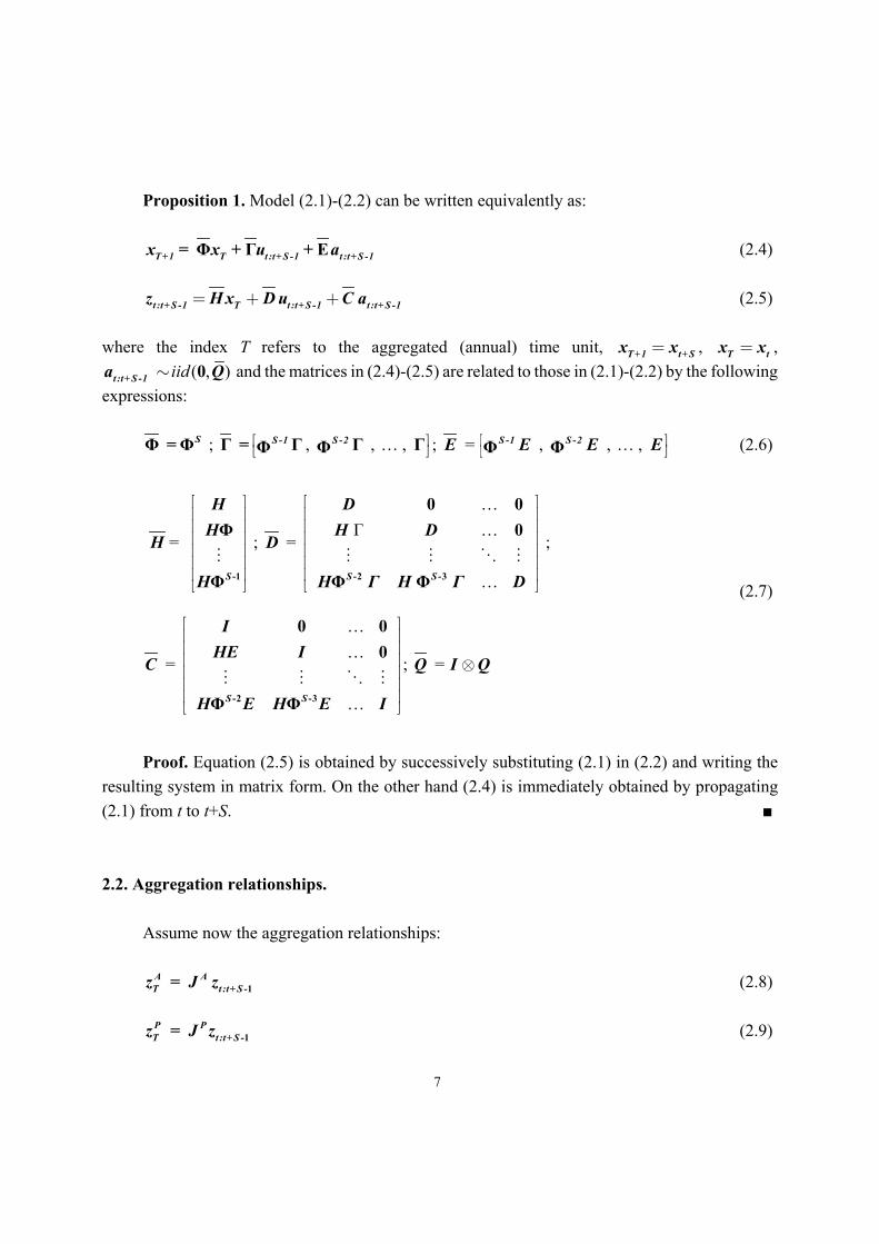
Proposition 1. Model (2.1)-(2.2) can be written equivalently as:

Φ Γ EΤ+1 Τ t :t+ S -1 t :t+ S -1x = x + u + a (2.4)

= + +t :t+ S -1 Τ t :t+ S -1 t :t+ S -1z H x D u C a (2.5)

where the index T refers to the aggregated (annual) time unit, =Τ+1 t+ Sx x , =Τ tx x ,

( , )iid 0∼t :t+ S -1a Q and the matrices in (2.4)-(2.5) are related to those in (2.1)-(2.2) by the following expressions:

Φ ΦS = ; , , … ,Γ Γ Γ ΓΦ Φ⎡ ⎤⎣ ⎦S -1 S -2 = ; = , , … , Φ Φ⎡ ⎤⎣ ⎦

S -1 S -2E E E E (2.6)

=

-1

Φ

Φ

⎡ ⎤⎢ ⎥⎢ ⎥⎢ ⎥⎢ ⎥⎢ ⎥⎢ ⎥⎣ ⎦

S

HH

H

H

;

… Γ …

=

…-2 -3

0 00

Φ Φ

⎡ ⎤⎢ ⎥⎢ ⎥⎢ ⎥⎢ ⎥⎢ ⎥⎢ ⎥⎣ ⎦

S S

DH D

D

H Γ H Γ D

;

(2.7)

……

=

…-2 -3

0 00

Φ Φ

⎡ ⎤⎢ ⎥⎢ ⎥⎢ ⎥⎢ ⎥⎢ ⎥⎢ ⎥⎣ ⎦

S S

IHE I

C

H E H E I

; = ⊗Q I Q

Proof. Equation (2.5) is obtained by successively substituting (2.1) in (2.2) and writing the resulting system in matrix form. On the other hand (2.4) is immediately obtained by propagating (2.1) from t to t+S. 2.2. Aggregation relationships.

Assume now the aggregation relationships:

1A AT t:t+ S -z = J z (2.8)

1P PT t:t+ S -z = J z (2.9)

8

where A

Tz and PTz denote, respectively, the vectors of annual and partially aggregated data observed

at year T, including the quarterly values at t, t+1, …, t+S-1. By ‘partially aggregated data’ we mean a sample combining all the observed annual and quarterly values. Note also that there always exists an aggregation relationship between the annual and partially aggregated series, see Lütkepohl (1987, Chapter 6): =A * P

T Tz J z (2.10) where (2.8)-(2.10) imply: =* P AJ J J . The structure of the aggregation matrices in (2.8), (2.9) and (2.10) obviously depends on the aggregation constraints and the nature of the variables. Following Di Fonzo (1990), there are four basic types of quarterly variables: flows, indices, beginning-of-period stocks or end-of-period stocks. Accordingly, the annual samples will be sums of quarterly values, averages or discrete beginning-of-period/end-of-period values. The following examples illustrate some common aggregation structures: Example 2.1: If all the variables considered are flows then = [ , , … , ]AJ I I I , meaning that each annual figure is the sum of the corresponding quarterly values. On the other hand,

[ ] = , , … ,AJ 0 0 I implies that the variables are end-of-period stocks, such that t+ S -1z is observed while the corresponding values at t, t+1, …, t+S-2 are not. Example 2.2: Assume that the first m1 variables in t :t+ S -1z , see (2.3), are annual flows, while the remaining m2 variables (m1+ m2=m) are quarterly values. In this case the partial aggregation matrix would be:

[ ]1 2 1 2( ) ( )m + S m S m + S m

⎡ ⎤⎢ ⎥⎢ ⎥⎢ ⎥⎢ ⎥= ⎢ ⎥⎢ ⎥⋅ × ⋅ ⋅⎢ ⎥⎢ ⎥⎢ ⎥⎢ ⎥⎣ ⎦

0 0 0

0 0 0 0

0 0 0 0

00 0 0 0

1 1

2

2

2

m m

mP

m

m

I I

IJ

I

I

(2.12) where mI is the m m× identity and the vectors of quarterly and partially observed values have the following structures:

9

[ ]1 2( ) 1S m + S m

11

1

1

1

⎡ ⎤⎢ ⎥⎢ ⎥⎢ ⎥⎢ ⎥⎢ ⎥⎢ ⎥= ⎢ ⎥⋅ ⋅ × ⎢ ⎥⎢ ⎥⎢ ⎥⎢ ⎥⎢ ⎥⎢ ⎥⎣ ⎦

1

2

1

2

1

2

mtmtmt+

t :t+ S - mt+

mt+ S -mt+ S -

zzzzz

zz

; [ ]1 2( ) 1m + S m

1 1

1

1

⎡ ⎤+ + +⎢ ⎥⎢ ⎥⎢ ⎥⎢ ⎥= ⎢ ⎥⋅ × ⎢ ⎥⎢ ⎥⎢ ⎥⎢ ⎥⎣ ⎦

…1 1 1

2

2

2

m m mt t+ t+ S -

mP tT m

t+

mt+ S -

z z zz

zz

z

(2.13) Example 2.3: Assuming again that all the variables are flows, the aggregation matrix *J in (2.10), transforming partially aggregated values into annual values, would be:

[ ]1 2 1 2( ) ( )m + m m + S m

⎡ ⎤⎢ ⎥= ⎢ ⎥× ⋅ ⎢ ⎥⎣ ⎦

0 0 0

01

2 2 2

*m

m m m

IJ

I I I (2.11)

2.3. Relationship between the quarterly, annual and partially aggregated models.

Under the previously stated conditions, the following result formalizes the relationship between the quarterly data model in the form (2.4)-(2.5) and the corresponding models for the annual and partially observed values:

Proposition 2. The models for ATz and P

Tz have the state equation (2.4) with the observation equations:

= + +A A A AT T t:t+ S -1 t :t+ S -1z H x D u C a (2.14)

1 1= + +P P P P

T T t:t+ S - t :t+ S -z H x D u C a (2.15) with:

= = = ; ;A A A A A AH J H D J D C J C (2.16)

; ;= = =P P P P P PH J H D J D C J C (2.17)

Proof. Trivial, as pre-multiplying (2.5) by JA and JP immediately yields (2.14) and (2.15) respectively.

10

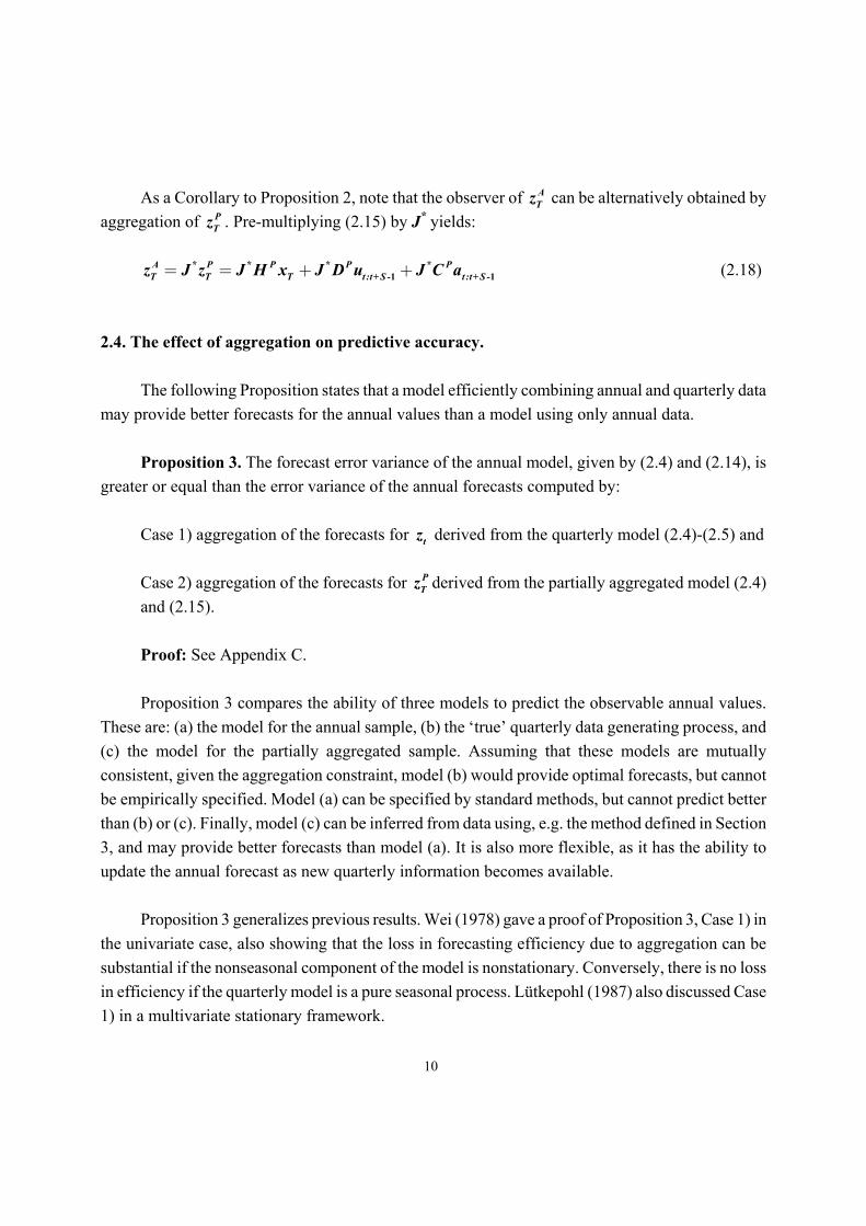
As a Corollary to Proposition 2, note that the observer of A

Tz can be alternatively obtained by aggregation of P

Tz . Pre-multiplying (2.15) by J* yields: 1 1= = + +A * P * P * P * P

T T T t:t+ S - t :t+ S -z J z J H x J D u J C a (2.18) 2.4. The effect of aggregation on predictive accuracy.

The following Proposition states that a model efficiently combining annual and quarterly data may provide better forecasts for the annual values than a model using only annual data.

Proposition 3. The forecast error variance of the annual model, given by (2.4) and (2.14), is greater or equal than the error variance of the annual forecasts computed by:

Case 1) aggregation of the forecasts for tz derived from the quarterly model (2.4)-(2.5) and

Case 2) aggregation of the forecasts for PTz derived from the partially aggregated model (2.4)

and (2.15). Proof: See Appendix C. Proposition 3 compares the ability of three models to predict the observable annual values.

These are: (a) the model for the annual sample, (b) the ‘true’ quarterly data generating process, and (c) the model for the partially aggregated sample. Assuming that these models are mutually consistent, given the aggregation constraint, model (b) would provide optimal forecasts, but cannot be empirically specified. Model (a) can be specified by standard methods, but cannot predict better than (b) or (c). Finally, model (c) can be inferred from data using, e.g. the method defined in Section 3, and may provide better forecasts than model (a). It is also more flexible, as it has the ability to update the annual forecast as new quarterly information becomes available. Proposition 3 generalizes previous results. Wei (1978) gave a proof of Proposition 3, Case 1) in the univariate case, also showing that the loss in forecasting efficiency due to aggregation can be substantial if the nonseasonal component of the model is nonstationary. Conversely, there is no loss in efficiency if the quarterly model is a pure seasonal process. Lütkepohl (1987) also discussed Case 1) in a multivariate stationary framework.

11

3. THE EFFECT OF AGGREGATION ON THE OBSERVABILITY OF A TIME SERIES MODEL

3.1. Characterization of the modes that become unobservable after aggregation. As shown in Section 2, the models for quarterly, annual and partially aggregated data share the state equation (2.4). Therefore, aggregation does not affect the states governing a dynamic system, but may reduce its observability. Comparing the observation equations (2.5) and (2.14)-(2.15) it is immediate to see that observability loss occurs in two ways: (a) the quarterly observer (2.5) has more observable signals than the aggregated observers (2.14)-(2.15), and (b) the matrices in (2.14)-(2.15) are non-linear functions of the matrices in (2.5), potentially decreasing the observability of some states. To further discuss this issue, we will particularize the general concept of observability (Anderson and Moore 1979, Appendix C) to the models and notation defined in Section 2.

Definition 1 (observability in the quarterly model). All the components in the quarterly model (2.1)-(2.2) are said to be observable i.i.f. there is no real vector 0≠w , with λ Φ w = w such that = 0Hw , where λ is the eigenvalue associated to the eigenvector w.

Definition 2 (unobservable modes in the annual model). Assuming that the variables are flows, so = [ , , … , ]AJ I I I , the annual model (2.4) and (2.14) has unobservable modes i.i.f. there exists a vector 0≠w , with λΦS w = w such that 0AH w = or, equivalently,

=0

S-1

i

0Φ∑ iH w = , see (2.6)-(2.7) and (2.16).

Under these conditions, Theorem 1 characterizes what components of the quarterly model become unobservable after annual aggregation.

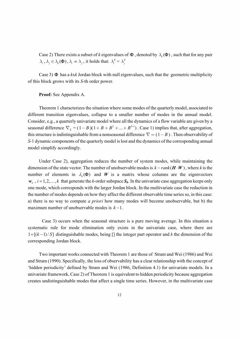
Theorem 1 (loss of observability in the annual model). Assuming that the quarterly model (2.1)-(2.2) is observable, the annual model (2.4) and (2.14) may include unobservable modes in any of the following cases:

Case 1) when the annual variables are flows, such that = [ , , … , ]AJ I I I , if there exists an

eigenvalue of Φ , λ , such that: 2 -11 + λ + λ + … + λ = 0S

12

Case 2) There exists a subset of k eigenvalues of Φ , denoted by ( )kλ Φ , such that for any pair

, ( ) , i j k i j λ λ λ λ λ∈ ≠Φ , it holds that: S Si j=λ λ

Case 3) Φ has a kxk Jordan block with null eigenvalues, such that the geometric multiplicity

of this block grows with its S-th order power.

Proof: See Appendix A. Theorem 1 characterizes the situation where some modes of the quarterly model, associated to

different transition eigenvalues, collapse to a smaller number of modes in the annual model. Consider, e.g., a quarterly univariate model where all the dynamics of a flow variable are given by a seasonal difference 2 -1= ( 1 )( 1 )S

S B B B … B∇ − + + + + . Case 1) implies that, after aggregation, this structure is indistinguishable from a nonseasonal difference ( 1 )B∇= − . Then observability of S-1 dynamic components of the quarterly model is lost and the dynamics of the corresponding annual model simplify accordingly.

Under Case 2), aggregation reduces the number of system modes, while maintaining the

dimension of the state vector. The number of unobservable modes is ( )k rank− ⋅H W , where k is the number of elements in ( )kλ Φ and W is a matrix whose columns are the eigenvectors

, 1, 2, ,i k= …iw that generate the k-order subspace Sk. In the univariate case aggregation keeps only one mode, which corresponds with the larger Jordan block. In the multivariate case the reduction in the number of modes depends on how they affect the different observable time series so, in this case: a) there is no way to compute a priori how many modes will become unobservable, but b) the maximum number of unobservable modes is 1k − .

Case 3) occurs when the seasonal structure is a pure moving average. In this situation a systematic rule for mode elimination only exists in the univariate case, where there are 1 [( 1) / ]k S+ − distinguishable modes, being [] the integer part operator and k the dimension of the corresponding Jordan block.

Two important works connected with Theorem 1 are those of Stram and Wei (1986) and Wei

and Stram (1990). Specifically, the loss of observability has a clear relationship with the concept of ‘hidden periodicity’ defined by Stram and Wei (1986, Definition 4.1) for univariate models. In a univariate framework, Case 2) of Theorem 1 is equivalent to hidden periodicity because aggregation creates undistinguishable modes that affect a single time series. However, in the multivariate case

13

hidden periodicity not always implies loss of observability; consider e.g., the situation where two modes with hidden periodicity affect two different time series. Also, the mode elimination rules discussed for cases 2) and 3) are coherent, in the univariate case, with Stram and Wei (1986, Theorems 4.1 and 3.1). After discussing the effect of aggregation over the quarterly model dynamics and its observability, it is important to characterize the uniqueness of the correspondence between the models for disaggregated and aggregated data. This is done in the following Theorem. Theorem 2 (correspondence between quarterly and annual models). If the quarterly model (2.4)-(2.5) is minimal and all its components are observable from annual data, then the annual model (2.4) and (2.14) is unique, allowing for similar transformations, minimal and observable.

Proof: See Appendix B. Note that in the last part of the proof we have assumed that the annual

variables are flows. Theorem 2 also holds for stock variables, but we do not have a proof for a general aggregation matrix.

The reciprocal proposition is not true in general. There are minimal and observable annual

models that necessary correspond to quarterly models with unobservable components. Assume e.g., that the model for annual data is an AR(1) with a negative parameter and that the seasonal frequency S is even. In this case, there is no high-frequency ARMA(1,1) process that adds to the annual AR(1) model because the S-th power of the transition matrix will always be positive, see (2.6). This result is closely related to Lemma 2 in Wei and Stram (1990).

3.2. Observability and fixed-interval smoothing.

Observability of a state obviously affects our ability to estimate it. In a SS framework, the method of choice for efficient state estimation is the fixed-interval smoother (Anderson and Moore 1979), which is a two-sided symmetric filter providing estimates of the first and second-order moments of the states conditional on all the information in the sample. The uncertainty of smoothed estimates critically depends on a property called “detectability”.

Definition 3 (detectability). A system is said to be detectable if their unobservable modes are

stationary.

14

Under these conditions, the following result characterizes the effect of undetectable modes on smoothed estimates.

Proposition 4. The variance of fixed-interval smoothing estimates of the states in models (2.4) and (2.14) or (2.15) is finite if and only if all the states are detectable.

Proof: See Appendix D. In time series disaggregation smoothing is typically employed to estimate the unobserved

quarterly values. Therefore detectability is a necessary and sufficient condition to estimate these values with bounded uncertainty while observability is a sufficient (not necessary) condition.

In time series disaggregation infinite smoothed variances would arise, for example, when the target variables are flows and their quarterly model includes seasonal roots in the unit circle. In this case the aggregated model has undetectable components and the variances of the estimates of seasonal components would be infinite. In practice this means that the annual series does not contain information about seasonal components and, therefore, if the quarterly indicators have seasonal component, it is advisable to remove them before disaggregation. 3.3. An algorithm to obtain the annual representation corresponding to a quarterly model. Combining Propositions 1 and 2 with Theorem 1 and other results from the SS literature, one can devise an algorithm to obtain the reduced-form model for a vector of annual data corresponding to any linear model for the quarterly values, allowing for a general aggregation constraint. This algorithm proceeds as follows: Step 1) Consider any linear and fixed-coefficients model for the quarterly data. Write the model in the innovations form (2.1)-(2.2). If the model can be written in VARMAX form, this can be done using the expressions given by Terceiro (1990, Section 2.1). In any other case, write the model in a general (non-innovations) state-space form and obtain the equivalent innovations representation (Casals, Sotoca and Jerez 1999, Theorem 1). Step 2) Obtain the equivalent quarterly representation (2.4)-(2.5) and the annual representation (2.4) and (2.14).

15

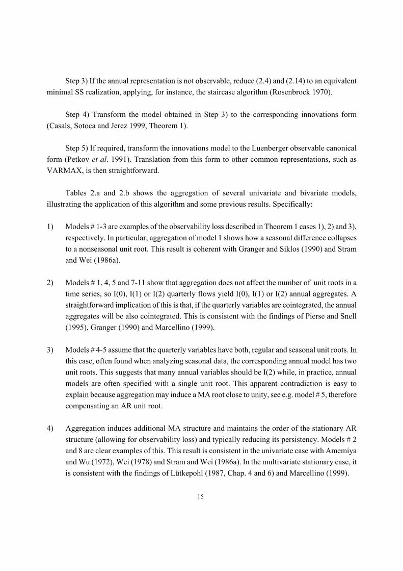
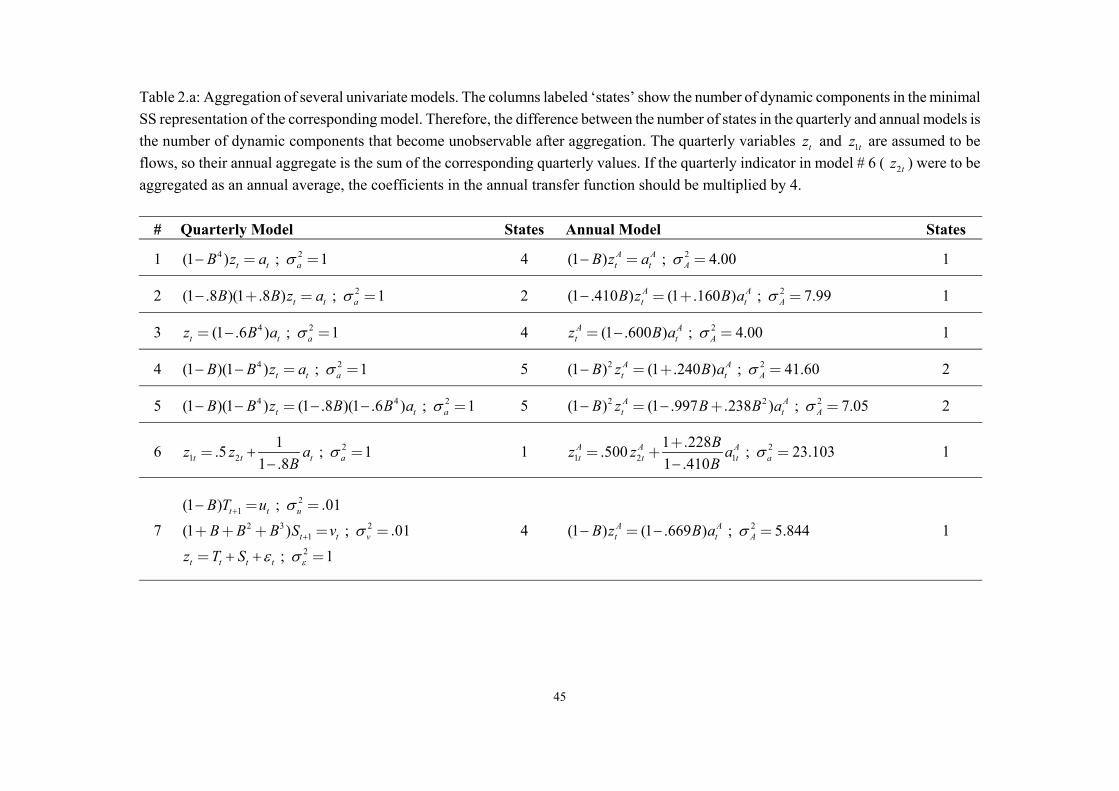
Step 3) If the annual representation is not observable, reduce (2.4) and (2.14) to an equivalent minimal SS realization, applying, for instance, the staircase algorithm (Rosenbrock 1970). Step 4) Transform the model obtained in Step 3) to the corresponding innovations form (Casals, Sotoca and Jerez 1999, Theorem 1). Step 5) If required, transform the innovations model to the Luenberger observable canonical form (Petkov et al. 1991). Translation from this form to other common representations, such as VARMAX, is then straightforward. Tables 2.a and 2.b shows the aggregation of several univariate and bivariate models, illustrating the application of this algorithm and some previous results. Specifically: 1) Models # 1-3 are examples of the observability loss described in Theorem 1 cases 1), 2) and 3),

respectively. In particular, aggregation of model 1 shows how a seasonal difference collapses to a nonseasonal unit root. This result is coherent with Granger and Siklos (1990) and Stram and Wei (1986a).

2) Models # 1, 4, 5 and 7-11 show that aggregation does not affect the number of unit roots in a

time series, so I(0), I(1) or I(2) quarterly flows yield I(0), I(1) or I(2) annual aggregates. A straightforward implication of this is that, if the quarterly variables are cointegrated, the annual aggregates will be also cointegrated. This is consistent with the findings of Pierse and Snell (1995), Granger (1990) and Marcellino (1999).

3) Models # 4-5 assume that the quarterly variables have both, regular and seasonal unit roots. In

this case, often found when analyzing seasonal data, the corresponding annual model has two unit roots. This suggests that many annual variables should be I(2) while, in practice, annual models are often specified with a single unit root. This apparent contradiction is easy to explain because aggregation may induce a MA root close to unity, see e.g. model # 5, therefore compensating an AR unit root.

4) Aggregation induces additional MA structure and maintains the order of the stationary AR

structure (allowing for observability loss) and typically reducing its persistency. Models # 2 and 8 are clear examples of this. This result is consistent in the univariate case with Amemiya and Wu (1972), Wei (1978) and Stram and Wei (1986a). In the multivariate stationary case, it is consistent with the findings of Lütkepohl (1987, Chap. 4 and 6) and Marcellino (1999).

16

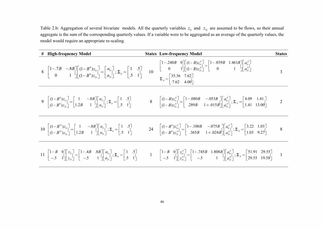
5) Models # 8-11 show that, if there is feedback in the quarterly frequency, there is feedback in

the annual frequency. 6) Model # 6 shows the annual model corresponding to a quarterly Chow-Lin AR(1) regression.

Therefore, this method is empirically justified only if the annual model relating the target variable and the indicator is a static regression with ARMA(1,1) errors.

7) Models # 7 and 11 show that the algorithm is not restricted to VARMAX or transfer functions,

as it can be applied to structural time series models (Harvey, 1989) and VARMAX echelon models. In general, it supports any model with an equivalent SS representation.

8) Finally, model # 10 shows that the algorithm can be applied to a general combination of

sampling and aggregation frequencies, as it shows how a monthly model aggregates to a quarterly VARMA.

[Insert Tables 2.a and 2.b]

17

4. AN EMPIRICAL METHOD TO MODEL TIME SERIES OBSERVED AT DIFFERENT FREQUENCIES.

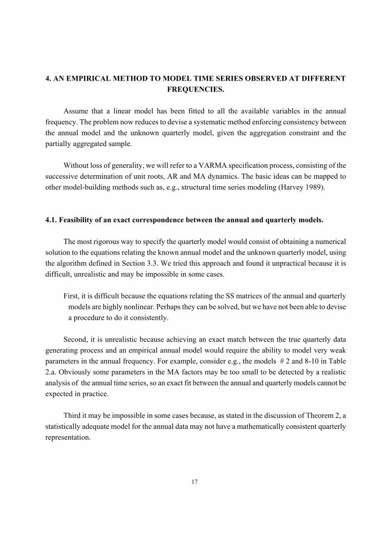
Assume that a linear model has been fitted to all the available variables in the annual frequency. The problem now reduces to devise a systematic method enforcing consistency between the annual model and the unknown quarterly model, given the aggregation constraint and the partially aggregated sample. Without loss of generality, we will refer to a VARMA specification process, consisting of the successive determination of unit roots, AR and MA dynamics. The basic ideas can be mapped to other model-building methods such as, e.g., structural time series modeling (Harvey 1989). 4.1. Feasibility of an exact correspondence between the annual and quarterly models.

The most rigorous way to specify the quarterly model would consist of obtaining a numerical solution to the equations relating the known annual model and the unknown quarterly model, using the algorithm defined in Section 3.3. We tried this approach and found it unpractical because it is difficult, unrealistic and may be impossible in some cases. First, it is difficult because the equations relating the SS matrices of the annual and quarterly

models are highly nonlinear. Perhaps they can be solved, but we have not been able to devise a procedure to do it consistently.

Second, it is unrealistic because achieving an exact match between the true quarterly data generating process and an empirical annual model would require the ability to model very weak parameters in the annual frequency. For example, consider e.g., the models # 2 and 8-10 in Table 2.a. Obviously some parameters in the MA factors may be too small to be detected by a realistic analysis of the annual time series, so an exact fit between the annual and quarterly models cannot be expected in practice. Third it may be impossible in some cases because, as stated in the discussion of Theorem 2, a statistically adequate model for the annual data may not have a mathematically consistent quarterly representation.

18

4.2. A method to enforce approximate consistency. If an exact correspondence between the quarterly and annual models cannot be expected to be found in practice, the only way forward would consist of devising a simple and fault-tolerant process to achieve an approximate fit and a diagnostic method to assess whether the quarterly model obtained is statistically adequate or not. The following procedure can be used to these purposes. Step 1) Annual modeling. Specify and estimate a model relating the target annual variable(s) with the annualized values of the quarterly indicator(s). Any model having an equivalent linear SS representation, such as e.g., a transfer function or VARMAX, is adequate for this purpose. Step 2) Decomposition of the quarterly indicator. Specify and estimate a quarterly model for the indicator(s). Use it to adjust undesired features of the quarterly indicator, such as seasonality and calendar effects. Step 3) Model specification.

Step 3.1) Set the VAR factor order of the quarterly model to be equal to that of the annual model and, particularly, constrain the number of unit roots to be the same. The foundation of this Step results from comparison of the quarterly model (2.4)-(2.5) and the annual model given by (2.4) and (2.14). As both models share the same state equation, they will have the same (stationary and nonstationary) autoregressive components. Step 3.2) Add a VMA(q) structure, with q n≤ , being n the size of the state vector in the annual model. This bound to MA dynamics results from the fact that, in a minimal SS representation, the size of the state vector is the maximum of p and q, being p the order of the VAR factor and q the order of the VMA factor.

Step 4) Estimation. Estimate the model specified in Steps 2) and 3) by maximum likelihood and prune insignificant parameters to obtain a parsimonious parametrization. Step 5) Diagnostics. Check the final quarterly model by obtaining the corresponding annual representation, using the algorithm described in Section 3.3, and then:

Step 5.1) compare this model with the one specified in Step 1) and Step 5.2) check whether it filters the annual data to white noise residuals.

Step 6) Forecasting accuracy check. If the sample is long enough, compare the out-of-the-

19

sample forecasts for the annual values produced by both, the tentative quarterly model and the annual model specified in Step 1). 4.3. Practical suggestions. We have applied the method described above to several real and simulated time series. These exercises provided some useful insights about the practical application of our method: First, a good characterization of unit roots in Step 1) is critical, as misspecification of these components impacts severely over the quality of final results (Tiao 1972). When in doubt over-differencing is safer than under-differencing, according to our experience. Second, the number of MA parameters specified in Step 3.2) may be excessive, depending on the sample size and number of time series. In this case, it is a good idea to constrain the MA matrices to be diagonal and, later, add off-diagonal parameters in a sequence of overfitting experiments. Third, when working with data coming from national accounts, we have often found that the annual variable (typically some component of GDP) has been measured for more years than the quarterly time series. In this situation the ability of SS methods to treat missing observations is an important advantage, as it allows using all the information available in these non-conformable samples. Last, the forecasting accuracy check proposed in Step 6) can be implemented by setting some within-the-sample values to missing and estimating them afterwards. We have found this alternative useful when the sample is too short to reserve some values for out-of-the-sample forecasting. The example in Section 5 illustrates how the last two ideas can be applied in practice.

20

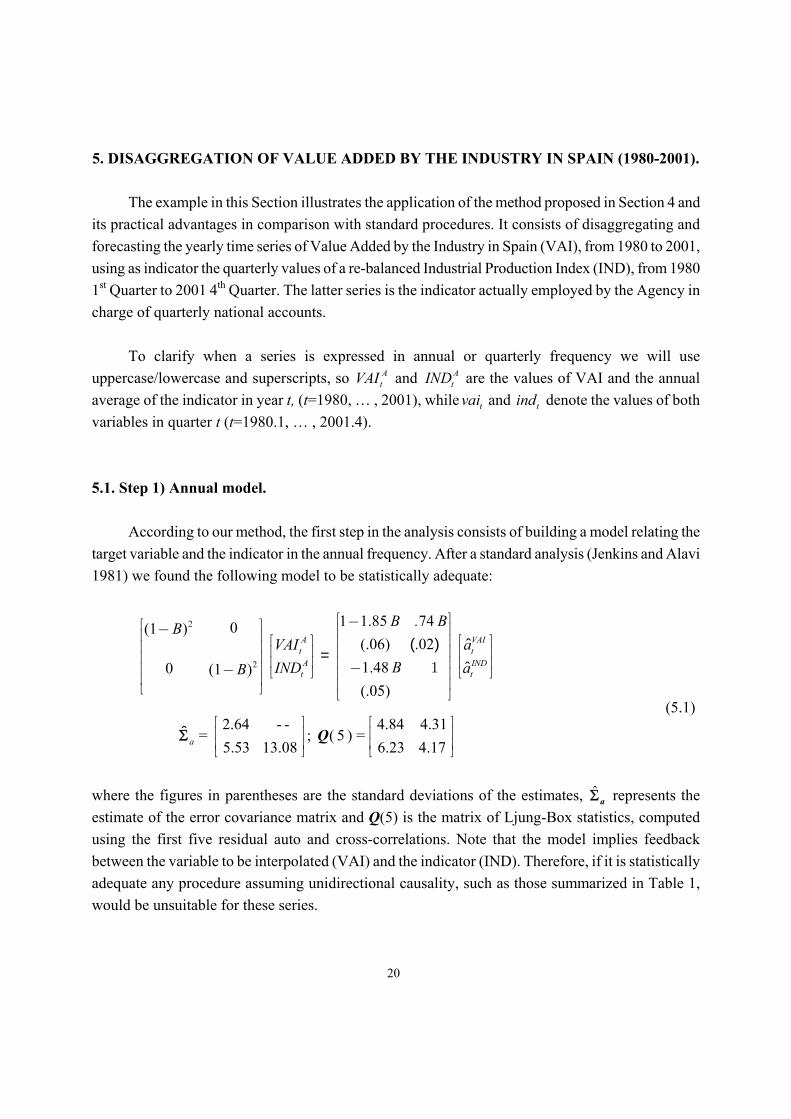
5. DISAGGREGATION OF VALUE ADDED BY THE INDUSTRY IN SPAIN (1980-2001).

The example in this Section illustrates the application of the method proposed in Section 4 and its practical advantages in comparison with standard procedures. It consists of disaggregating and forecasting the yearly time series of Value Added by the Industry in Spain (VAI), from 1980 to 2001, using as indicator the quarterly values of a re-balanced Industrial Production Index (IND), from 1980 1st Quarter to 2001 4th Quarter. The latter series is the indicator actually employed by the Agency in charge of quarterly national accounts.

To clarify when a series is expressed in annual or quarterly frequency we will use uppercase/lowercase and superscripts, so A

tVAI and AtIND are the values of VAI and the annual

average of the indicator in year t, (t=1980, … , 2001), while tvai and tind denote the values of both variables in quarter t (t=1980.1, … , 2001.4). 5.1. Step 1) Annual model.

According to our method, the first step in the analysis consists of building a model relating the target variable and the indicator in the annual frequency. After a standard analysis (Jenkins and Alavi 1981) we found the following model to be statistically adequate:

2

2

1 1.85 740(1 ) (.06) .02

1.48 0 (1 ) (.05)

2.64 - - 4.84 4.31 = ; ( 5 ) =

5.53 13.08 6.2

A VAIt tA IND

t t

a

B . BBVAI a

BIND aB( ) ˆ

ˆ

ˆ

=

⎡ ⎤−⎡ ⎤− ⎢ ⎥⎢ ⎥ ⎡ ⎤ ⎡ ⎤⎢ ⎥⎢ ⎥ ⎢ ⎥ ⎢ ⎥⎢ ⎥⎢ ⎥ ⎢ ⎥ ⎢ ⎥⎢ ⎥−⎢ ⎥− ⎣ ⎦ ⎣ ⎦⎢ ⎥⎢ ⎥ ⎢ ⎥⎣ ⎦ ⎣ ⎦

⎡ ⎤⎢ ⎥⎢ ⎥⎣ ⎦

1

Σ Q3 4.17

⎡ ⎤⎢ ⎥⎢ ⎥⎣ ⎦

(5.1) where the figures in parentheses are the standard deviations of the estimates, ˆ

aΣ represents the estimate of the error covariance matrix and Q(5) is the matrix of Ljung-Box statistics, computed using the first five residual auto and cross-correlations. Note that the model implies feedback between the variable to be interpolated (VAI) and the indicator (IND). Therefore, if it is statistically adequate any procedure assuming unidirectional causality, such as those summarized in Table 1, would be unsuitable for these series.

21

Model (5.1) provides precise clues about dynamics of both variables in the quarterly frequency. According to the method outlined in Section 4.2, the quarterly model would have a non-stationary AR structure with two unit roots for each series and an MA term with a maximum order of 4, because the minimal SS representation of model (5.1) requires four state variables.

5.2. Step 2) Decomposition of the quarterly indicator.

The second step requires modeling the indicator in the quarterly frequency to estimate the components useful for disaggregation. To this end, we will use the following model:

4 4 2

ˆ1.02 1.85 5.94(.03) (.35) (1.72)

ˆ ˆ ˆ(1 )(1 ) (1 .83 ) ; 3.21 ; (15) = 12.80(.06)

92.4t t t t t

t t a

ind L E S N

B B N B a Qσ

= − − +

− − = − = (5.2)

where tL is the number of non-holidays in quarter t, tE is a dummy variable to account for Easter effects and 92.4

tS is an intervention variable modeling a persistent level change from 1992 4th Quarter onwards.

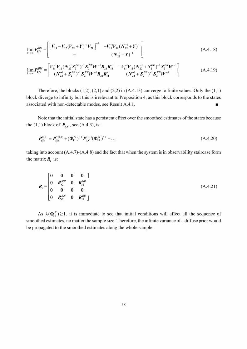
Model (5.2) implies (Casals, Jerez and Sotoca 2002) that the indicator can be split into: (a) trend, (b) seasonal component, (c) irregular component, (d) calendar effects associated to the number of non-holidays and Easter and (e) the step 1992 4th Quarter effect. Figure 1 shows these components. In the light of previous results, components (b) and (d) are useless for disaggregation and will be accordingly deleted. Addition of the remaining components yields a time series that can be interpreted as a seasonally and calendar-adjusted quarterly indicator of VAI. [Insert Figure 1] 5.3. Steps 3) and 4) Specification and estimation of the quarterly model.

Building on previous steps, we now estimate a doubly integrated VMA(4) process for VAI and the adjusted indicator in the quarterly frequency, taking into account that VAI values are annually aggregated. After pruning insignificant parameters we obtained the following model:

22

2

2

(1 ) 1 1.48 .36 .044.06 - - (.06) (.06) (.003)

; =.40 3.64.84 1 .78(1 )

(.06) (.02)

2

vait t

indt t

B B B Bvai a

B Bind aB

ˆ ˆˆ

⎡ ⎤ ⎡ ⎤− − +⎢ ⎥ ⎢ ⎥⎢ ⎥ ⎡ ⎤⎢ ⎥⎡ ⎤ ⎡ ⎤⎢ ⎥ ⎢ ⎥⎢ ⎥⎢ ⎥ ⎢ ⎥=⎢ ⎥ ⎢ ⎥⎢ ⎥⎢ ⎥ ⎢ ⎥− −−⎢ ⎥ ⎣ ⎦⎢ ⎥⎢ ⎥⎣ ⎦ ⎣ ⎦⎢ ⎥ ⎢ ⎥⎢ ⎥ ⎢ ⎥⎣ ⎦⎣ ⎦

0

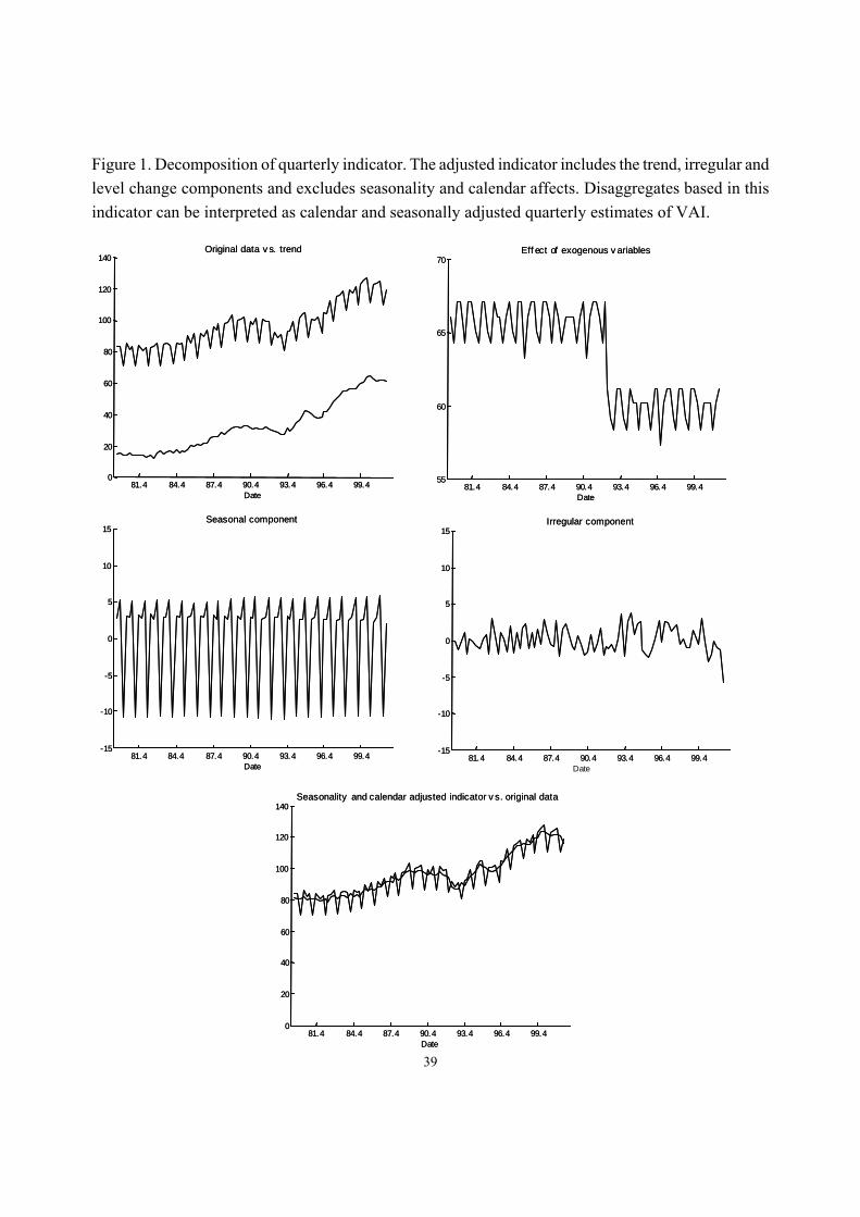
0 aΣ (5.3) where tind denotes the adjusted indicator. Finally, by applying a fixed-interval smoothing to the sample (Casals Jerez and Sotoca 2000), we obtain the disaggregates and forecasts shown in Figure 2. [Insert Figure 2] 5.4. Step 5) Diagnostics. Using the algorithm described in Section 3.3, we now obtain the annual representation corresponding to model (5.3):

(5.4)

2

2

(1 ) 1.52 .23 70 .10(1 ) 1.18 .19 .14 .07

2.54 - - 7.38 7.81 = ; ( 5 ) =

5.53 13.79 9.49 8.48

A VAIt tA INDt t

VAIB B B . B + B aB B B B BIND a

ˆ

ˆ

ˆ

=

⎡ ⎤ ⎡ ⎤⎡ ⎤ ⎡ ⎤− − −⎢ ⎥ ⎢ ⎥⎢ ⎥ ⎢ ⎥⎢ ⎥ ⎢ ⎥⎢ ⎥ ⎢ ⎥− − − + −⎢ ⎥ ⎢ ⎥⎣ ⎦ ⎣ ⎦ ⎣ ⎦⎣ ⎦

⎡ ⎤ ⎡ ⎤⎢ ⎥ ⎢⎢ ⎥ ⎢⎣ ⎦ ⎣ ⎦

2 2

2 2

0 10 1

Σa Q ⎥⎥

where

AtIND denotes the annual average of the adjusted indicator. Models (5.4) and (5.1) differ

mainly in the additional second-order MA parameters in (5.4). We tried to fit an annual model including these parameters and the corresponding estimates resulted insignificant. Then, this additional MA structure may be due to the disaggregated indicator information included in (5.3) and excluded in (5.1). On the other hand, the residuals are stationary, normal and do not show important autocorrelations. Therefore, we accept that model (5.3) is statistically adequate and roughly conformable with (5.1). The results already shown in this example show that our method can be applied to real disaggregation problems. The remaining Subsections highlight its unique advantages when dealing with non-conformable samples and in terms of forecasting power.

23

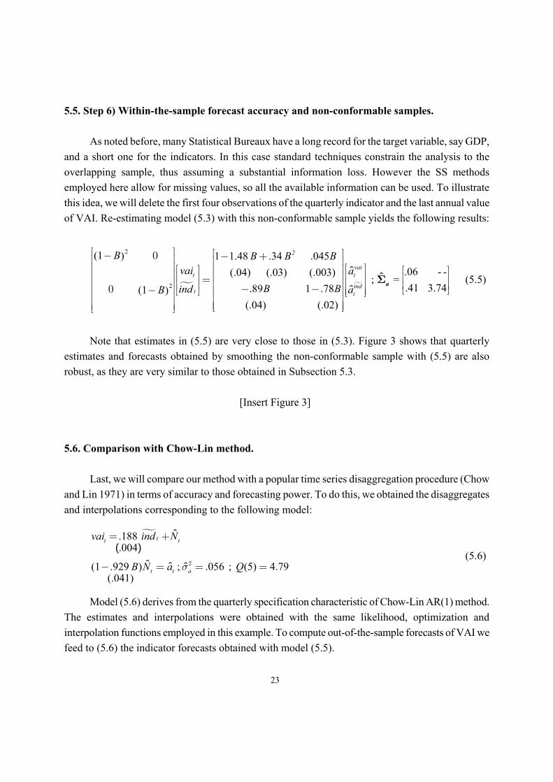
5.5. Step 6) Within-the-sample forecast accuracy and non-conformable samples.

As noted before, many Statistical Bureaux have a long record for the target variable, say GDP, and a short one for the indicators. In this case standard techniques constrain the analysis to the overlapping sample, thus assuming a substantial information loss. However the SS methods employed here allow for missing values, so all the available information can be used. To illustrate this idea, we will delete the first four observations of the quarterly indicator and the last annual value of VAI. Re-estimating model (5.3) with this non-conformable sample yields the following results:

2

2

(1 ) 1 1.48 .34 .045.06 - - (.04) (.03) (.003)

; =.41 3.74.89 1 .78(1 )

(.04) (.02)

2

vait t

indt t

B B B Bvai a

B Bind aB

ˆ ˆˆ

⎡ ⎤ ⎡ ⎤− − +⎢ ⎥ ⎢ ⎥⎢ ⎥ ⎡ ⎤⎢ ⎥⎡ ⎤ ⎡ ⎤⎢ ⎥ ⎢ ⎥⎢ ⎥⎢ ⎥ ⎢ ⎥=⎢ ⎥ ⎢ ⎥⎢ ⎥⎢ ⎥ ⎢ ⎥− −−⎢ ⎥ ⎣ ⎦⎢ ⎥⎢ ⎥⎣ ⎦ ⎣ ⎦⎢ ⎥ ⎢ ⎥⎢ ⎥ ⎢ ⎥⎣ ⎦⎣ ⎦

0

0Σa (5.5)

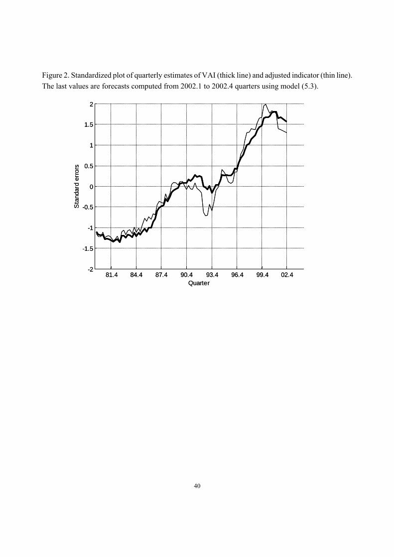
Note that estimates in (5.5) are very close to those in (5.3). Figure 3 shows that quarterly estimates and forecasts obtained by smoothing the non-conformable sample with (5.5) are also robust, as they are very similar to those obtained in Subsection 5.3. [Insert Figure 3] 5.6. Comparison with Chow-Lin method.

Last, we will compare our method with a popular time series disaggregation procedure (Chow and Lin 1971) in terms of accuracy and forecasting power. To do this, we obtained the disaggregates and interpolations corresponding to the following model:

.188 .004

tt tvai ind N( )= +

(5.6) (1 .929 ) ; .056 ; (5) 4.79

(.041)t t aB N a Qˆ ˆ σ− = = =2

Model (5.6) derives from the quarterly specification characteristic of Chow-Lin AR(1) method.

The estimates and interpolations were obtained with the same likelihood, optimization and interpolation functions employed in this example. To compute out-of-the-sample forecasts of VAI we feed to (5.6) the indicator forecasts obtained with model (5.5).

24

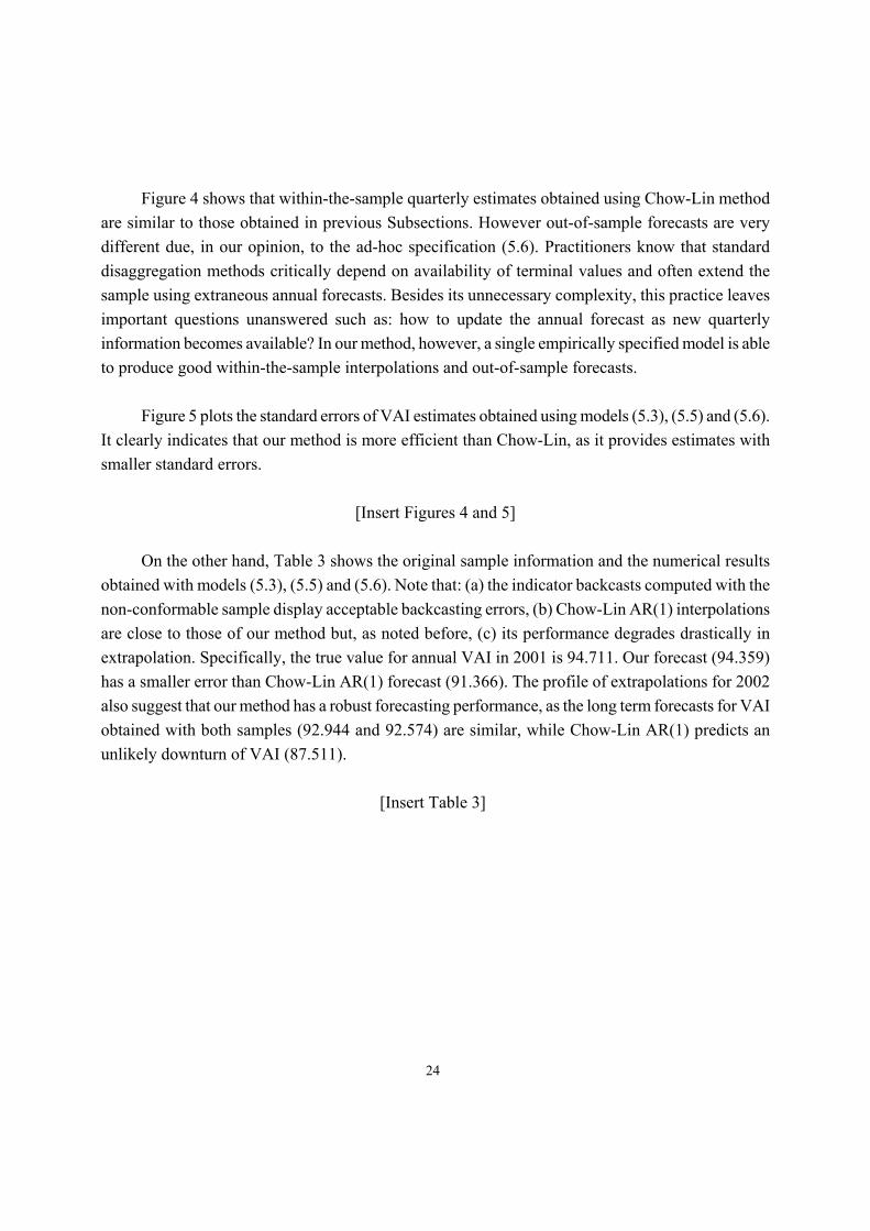
Figure 4 shows that within-the-sample quarterly estimates obtained using Chow-Lin method are similar to those obtained in previous Subsections. However out-of-sample forecasts are very different due, in our opinion, to the ad-hoc specification (5.6). Practitioners know that standard disaggregation methods critically depend on availability of terminal values and often extend the sample using extraneous annual forecasts. Besides its unnecessary complexity, this practice leaves important questions unanswered such as: how to update the annual forecast as new quarterly information becomes available? In our method, however, a single empirically specified model is able to produce good within-the-sample interpolations and out-of-sample forecasts.

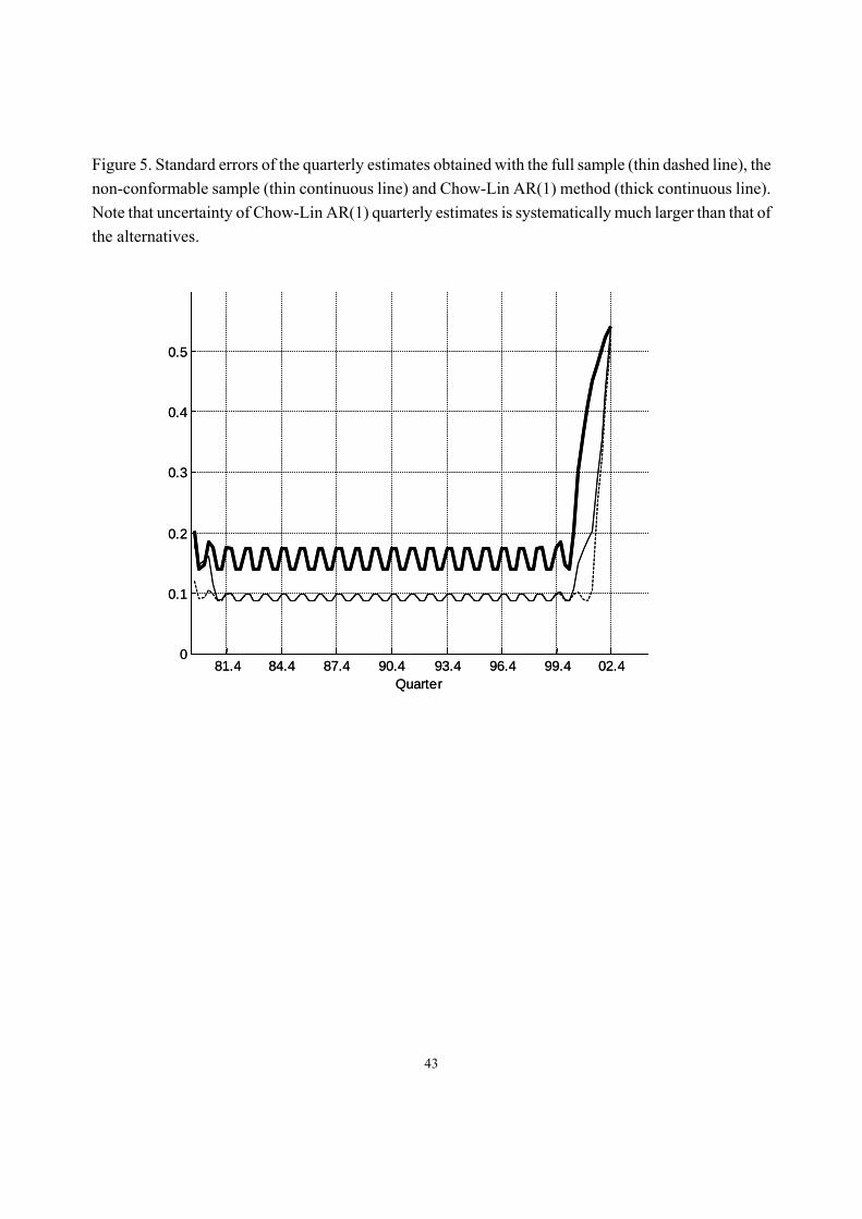
Figure 5 plots the standard errors of VAI estimates obtained using models (5.3), (5.5) and (5.6).

It clearly indicates that our method is more efficient than Chow-Lin, as it provides estimates with smaller standard errors.

[Insert Figures 4 and 5]

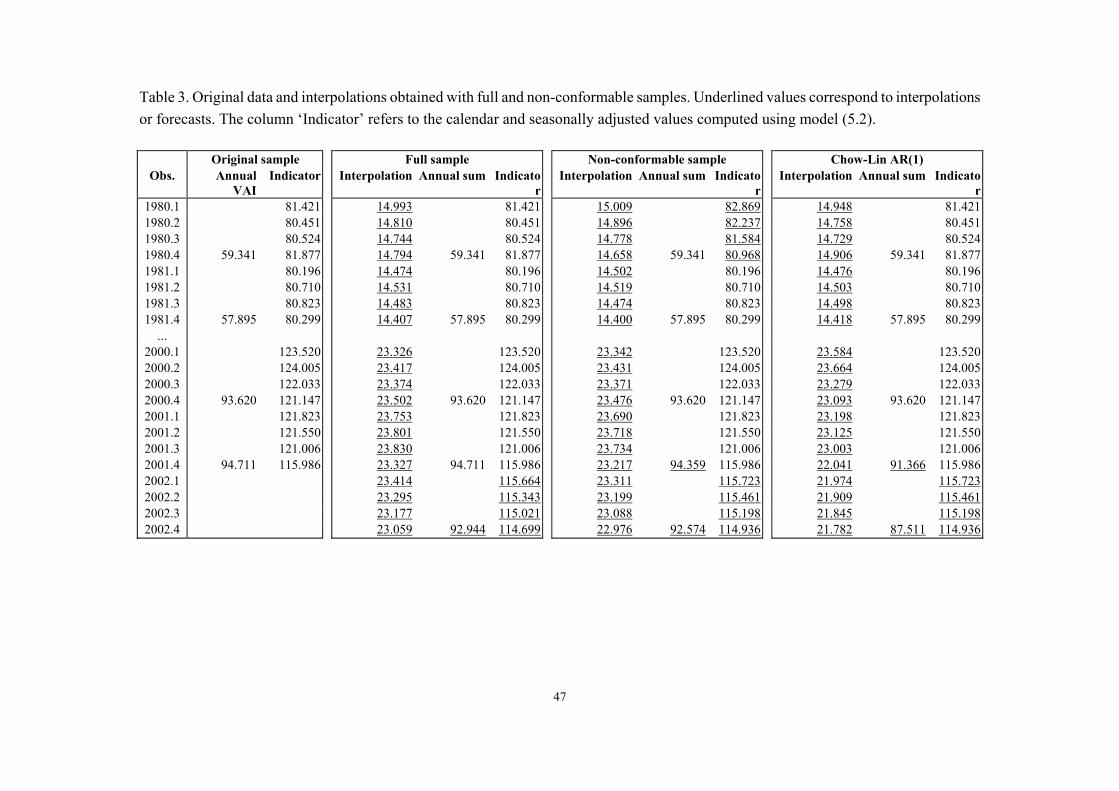
On the other hand, Table 3 shows the original sample information and the numerical results

obtained with models (5.3), (5.5) and (5.6). Note that: (a) the indicator backcasts computed with the non-conformable sample display acceptable backcasting errors, (b) Chow-Lin AR(1) interpolations are close to those of our method but, as noted before, (c) its performance degrades drastically in extrapolation. Specifically, the true value for annual VAI in 2001 is 94.711. Our forecast (94.359) has a smaller error than Chow-Lin AR(1) forecast (91.366). The profile of extrapolations for 2002 also suggest that our method has a robust forecasting performance, as the long term forecasts for VAI obtained with both samples (92.944 and 92.574) are similar, while Chow-Lin AR(1) predicts an unlikely downturn of VAI (87.511). [Insert Table 3]

25

6. CONCLUDING REMARKS. This paper makes a twofold contribution to the literature about aggregation of time series: First, it encompasses many previous results about: (a) the effect of aggregation on the dynamics of ARIMA (Amemiya and Wu, 1972, Brewer, 1973, Stram and Wei, 1986) and VARMA processes (Marcellino, 1999), (b) the observability loss due to aggregation (Wei and Stram, 1990) and (c) the negative effect of aggregation on forecasting accuracy in the univariate (Wei, 1978) and multivariate case (Lütkepohl, 1987). Second, it proposes a method to build a high-frequency model using a partially aggregated sample, allowing for general sampling frequencies and aggregation constraints. This method emphasizes the idea that the quarterly model should be both, consistent with a statistically adequate model fitted to annual data, and compliant with standard diagnostics. These two requirements define the empirical foundations of our method. We heavily used SS techniques to solve the specification, estimation, interpolation and forecasting issues that arise when sampling is done at different frequencies. In comparison with other alternatives, the SS approach has clear advantages as it provides: (a) a high degree of independence from particular model families, as the SS representation encompasses most common time series models, (b) standard and well-tested procedures to solve the estimation, interpolation and forecasting issues arising in this framework, and (c) the ability to treat samples with missing values, which may be important when the samples are not conformable.

The procedures described in this article are implemented in a MATLAB toolbox for time series modeling called E4, which can be downloaded at www.ucm.es/info/icae/e4. The source code for all the functions in the toolbox is freely provided under the terms of the GNU General Public License. This site also includes a complete user manual and other materials.

26

REFERENCES. Amemiya, T. and R.Y. Wu (1972), “The Effect of Aggregation on Prediction in the Autoregressive

Model,” Journal of the American Statistical Association, 339, 628-632. Anderson, B.D.O. and J.B. Moore (1979), Optimal Filtering, Prentice-Hall, Englewood Cliffs, NJ. Ansley, C. F. and R. Kohn (1983), “Exact Likelihood of Vector Autoregressive-Moving Average

Process with Missing or Aggregated Data,” Biometrika, 70, 1, 275–278. Ansley, C. F. and R. Kohn (1989), “Filtering and smoothing in state space models with partially

diffuse initial conditions,” Journal of Time Series Analysis, 11, 275–293. Boot, J.G.C., W. Feibes and J.H.C. Lisman (1967), “Further Methods of Derivation of Quarterly

Figures from Annual Data,” Applied Statistics, 16, 65-75. Bitmead, R.R., M.R. Gevers, I.R. Petersen and R.J. Kaye (1985), “Monotonicity and Stabilizability

Properties of the Solutions of the Riccati Difference Equation: Propositions, Lemmas, Theorems, Fallacious Conjectures and Counterexamples” System Control Letters, 5, 309-315.

Brewer, K.W. (1973), “Some Consequences of Temporal Aggregation and Systematic Sampling for

ARMA and ARMAX Models,” Journal of Econometrics, 1, 133-154. Casals, J., Sotoca, S. and Jerez, M. (1999), “A Fast and Stable Method to Compute the Likelihood of

Time Invariant State-Space Models,” Economics Letters, 65, 329-337. Casals, J., Jerez, M., and Sotoca, S. (2000), “Exact Smoothing for Stationary and Nonstationary

Time Series,” International Journal of Forecasting, 16, 1, 59-69. Casals, J., Jerez, M., and Sotoca, S. (2002), “An Exact Multivariate Model-based Structural

Decomposition,” Journal of the American Statistical Association, 97, 458, 553-564. Chow, G.C. and A.L. Lin (1971), “Best Linear Unbiased Interpolation, Distribution and

Extrapolation of Time Series by Related Series,” The Review of Economics and Statistics, 53, 372-375.

De Jong, P. (1991), “The diffuse Kalman filter,” The Annals of Statistics, 19, 1073–1083.

27

Denton, F.T. (1971), “Adjustment of Monthly or Quarterly Series to Annual Totals: An Approach Based on Quadratic Minimization,” Journal of the American Statistical Association, 66, 333, 99-102.

Di Fonzo, T. (1990), “The Estimation of M Disaggregate Time Series when Contemporaneous and

Temporal Aggregates are Known,” The Review of Economics and Statistics, 72, 1, 178-182. Fernández, R.B. (1981), “A Methodological Note on the Estimation of Time Series,” The Review of

Economics and Statistics, 63, 471-476. Granger, C.W.J. (1990), “Aggregation of Time-Series Variables: A Survey,” in Disaggregation in

Econometric Modelling, eds. T. Barker and M.H. Pesaran, pp. 17-34, Routledge, London. Granger, C.W.J. and P.R. Siklos (1995), “Systematic Sampling, Temporal Aggregation, Seasonal

Adjustment and Cointegration. Theory and Evidence,” Journal of Econometrics, 66, 357-369. Harvey, A.C. and R.G. Pierse (1984), “Estimating Missing Observations in Economic Time Series,”

Journal of the American Statistical Association, 79, 385, 125-131. Harvey, A.C. (1989), Forecasting, Structural Time Series Models and the Kalman Filter, Cambridge

(UK): Cambridge University Press. Jenkins, G.M. and A.S. Alavi (1981), “Some Aspects of Modelling and Forecasting Multivariate

Time Series,” Journal of Time Series Analysis, 2, 1, 1-47. Kalman, R.E. (1963), “Mathematical Description of Linear Systems,” SIAM Journal of Control, 1,

152-192. Litterman, R.B. (1983), “A Random Walk, Markov Model for the Distribution of Time Series,”

Journal of Business and Economic Statistics, 1, 169-173. Lütkepohl, H. (1987), Forecasting Aggregated Vector ARMA Processes, Springer-Verlag, Berlin. Marcellino, M. (1999), “Some Consequences of Temporal Aggregation in Empirical Analysis,”

Journal of Business and Economic Statistics, 1, 129-136. Onof, C., H. Wheater, D. Chandler, V. Isham, D.R. Cox, A. Kakou, P. Northrop, L. Oh and I.

Rodriguez-Iturbe (2000), “Spatial-temporal rainfall fields: modelling and statistical aspects,”

28

Hydrology and Earth System Sciences, 4, 4, 581-601. Petkov, P. Hr., N.D. Christov and M.M. Konstantinov (1991). Computational Methods for Linear

Control Systems, Prentice-Hall, Englewood Cliffs, New Jersey. Pierse, R.G. and A.J. Snell (1995), “Temporal Aggregation and the Power of Tests for a Unit Root,”

Journal of Econometrics, 65, 333-345. Rosenbrock, M.M. (1970), State-Space and Multivariable Theory, John Wiley, New York. Stram, D.O. and W.W.S. Wei (1986), “Temporal Aggregation in the ARIMA process,” Journal of

Time Series Analysis, 7, 4, 279-292. Tiao, G.C. (1972), “Asymptotic Behavior of Time Series Aggregates,” Biometrika, 59, 521-531. Terceiro, J. (1990), Estimation of Dynamic Econometric Models with Errors in Variables, Springer-

Verlag, Berlin. Wei, W.W.S. (1978), “Some Consequences of Temporal Aggregation in Seasonal Time Series

Models” In Zellner, A. (ed.), Seasonal Analysis of Economic Time Series, published by the U.S. Bureau of the Census, Government Printing Office, 433-448.

Wei, W.W.S. and D.O. Stram (1990), “Disaggregation of Time Series Models,” Journal of the Royal

Statistical Society, B Series, 52, 3, 453-467.

29

APPENDIX A: PROOF OF THEOREM 1

According to definitions 1) and 2), the annual model (2.4) and (2.14) has unobservable modes if there exists at least a vector ≠ 0w such that λ=S w wΦ and: 1

=0

=S-

i

0∑ iH w Φ (A.1.1)

A.1.1 Proof of Case 1). Expression (A.1.1) implies:

+ + + = 0… SHw H w H w H w2 −1Φ Φ Φ (A.1.2) If w is an eigenvector of Φ , then it is also an eigenvector of the powers of Φ , so λ ( = 1, 2, )i i i …w = wΦ and, therefore:

2 1 2 -1+ + + = 1+ + + =S- Sλ λ λ λ λ λ 0⎡ ⎤+⎢ ⎥⎣ ⎦… …Hw H w H w H w Hw (A.1.3)

but, as the quarterly model is observable, then 0≠Hw and (A.1.3) holds i.i.f. 2 -11+ + + = 0Sλ λ λ+… A.1.2 Proof of Case 2).

Under the conditions of Case 2), the k eigenvectors associated to ( )λk Φ generate a subspace,

denoted by λ,kS , such that for any λ,k∈w S , it holds that S λw = wΦ , where λ λ λ ( )λSki i,= ∀ ∈ Φ .

Let IS be the intersection between λ,kS and the null space of matrix H, then

I λ,kdim dim null k rank( ) ( ) ( )⎡ ⎤= ∩ = −⎣ ⎦S S H HW , where W is a matrix which columns are the eigenvectors spanning λ,kS . In the univariate case, the number of unobservable modes is exactly

Idim k rank k( ) ( )= − = −1S HW , because H is a row matrix and the quarterly model is observable. In the multivariate case there is no exact rule but, in general, k rank( )− HW modes become unobservable and the maximum number of lost modes is k −1 .

30

A.1.3 Proof of Case 3).

Under the conditions of Case 3), it is easy to see that the S-th power of any k-dimension Jordan block with null eigenvalues breaks into several blocks. The dimension of the larger sub-block will then be [ ]1 1)+ k - /S( , where ‘[]’ denotes the integer part of a real argument.

Fragmentation of the Jordan block implies an increase in the geometric multiplicity associated

to the null eigenvalues, so there are several linearly independent eigenvectors associated to each null eigenvalue. This situation is therefore similar to the one analyzed in Case 2).

31

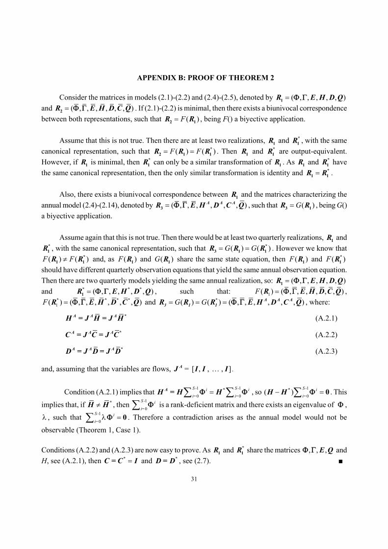
APPENDIX B: PROOF OF THEOREM 2

Consider the matrices in models (2.1)-(2.2) and (2.4)-(2.5), denoted by ( , , , , , )=1R E H D QΦ Γ and ( , , , , , , )=2R E H D C QΦ Γ . If (2.1)-(2.2) is minimal, then there exists a biunivocal correspondence between both representations, such that ( )F=2 1R R , being F() a biyective application.

Assume that this is not true. Then there are at least two realizations, 1R and 1

*R , with the same canonical representation, such that ( ) ( )F F= =2 1 1

*R R R . Then 1R and 1*R are output-equivalent.

However, if 1R is minimal, then 1*R can only be a similar transformation of 1R . As 1R and 1

*R have the same canonical representation, then the only similar transformation is identity and =1 1

*R R . Also, there exists a biunivocal correspondence between 1R and the matrices characterizing the

annual model (2.4)-(2.14), denoted by ( , , , , , , )=3A A AR E H D C QΦ Γ , such that ( )G=3 1R R , being G()

a biyective application. Assume again that this is not true. Then there would be at least two quarterly realizations, 1R and

1*R , with the same canonical representation, such that ( ) ( )G G= =3 1 1

*R R R . However we know that ( ) ( )F F≠1 1

*R R and, as ( )F 1R and ( )G 1R share the same state equation, then ( )F 1R and ( )F 1*R

should have different quarterly observation equations that yield the same annual observation equation. Then there are two quarterly models yielding the same annual realization, so: ( , , , , , )=1R E H D QΦ Γ and ( , , , , , )=1

* * *R E H D QΦ Γ , such that: 1( ) ( , , , , , , )F =R E H D C QΦ Γ ,

1( ) ( , , , , , , )F =* * * *R E H D C QΦ Γ and ( ) ( ) ( , , , , , , )G G= = =* A A A3 1 1R R R E H D C QΦ Γ , where:

A A A *H = J H = J H (A.2.1)

A A A *C = J C = J C (A.2.2)

A A A *D = J D = J D (A.2.3)

and, assuming that the variables are flows, = [ , , … , ]AJ I I I .

Condition (A.2.1) implies that 1 1

0 0

S - S -i ii= i=

=∑ ∑A *H = H HΦ Φ , so 1

0( ) S- i

i=− =∑ 0*H H Φ . This

implies that, if ≠ *H H , then 1

0

S- ii=∑ Φ is a rank-deficient matrix and there exists an eigenvalue of Φ ,

λ , such that 1

0

S- ii=λ =∑ 0Φ . Therefore a contradiction arises as the annual model would not be

observable (Theorem 1, Case 1). Conditions (A.2.2) and (A.2.3) are now easy to prove. As 1R and 1

*R share the matrices , , ,E QΦ Γ and H, see (A.2.1), then =*C = C I and *D = D , see (2.7).

32

APPENDIX C: PROOF OF PROPOSITION 3

A.3.1. Previous results.

Result A.3.1. Consider the algebraic Riccati equation of the Kalman filter: = −T T T

t t tt+1 t t t -1P P + EQE K B KΦ Φ (A.3.1) where: ( )= -1T

t tt t -1K P + EQ BΦ Η (A.3.2) = T

t t t -1B P + QΗ Η (A.3.3)

Under these conditions, if ≥*

t t -1 t t -1P P and ≥*Q Q then ≥*t+1 t t+1 tP P . See the proof in Bitmead

et al. (1985) Result A.3.2. Let be M a ( *m m× ) matrix where ( *rank m) =M with *m m< , and A, a symmetric positive-definite ( m m× ) matrix, with (rank m) =A . Under these conditions: − ( ) ≥ 0-1A Μ ΜA Μ ΜΤ Τ (A.3.4) *[rank m m− ( ) ] = −-1A Μ ΜA Μ ΜΤ Τ (A.3.5) Proof. It is immediate to see that: ( ) ( ) − ( ) = − = − −-1 T TA Μ ΜA Μ Μ A CAC I C A I CΤ Τ (A.3.6) where = ( )-1C Μ ΜA Μ ΜA−1 −1Τ Τ . Therefore, positive-definiteness of A assures that ( ) ( )− − TI C A I C is a positive-definite matrix also. A.3.2. Proof of Proposition 3. Case 1) Consider the high-frequency model in the stacked form (2.4)-(2.5). The k-step ahead forecast error variance is given by: ( )var Ω = 1

T TK T T + K - Te P + CQCΗ Η (A.3.7)

where T is the forecast origin and ΩT denotes the quarterly information available at time T. According to (A.3.7), the variance of the annual forecast obtained by aggregation would be:

33

( )( ) ( )var varΩ = Ω

TA A AK T K Te J e J (A.3.8)

On the other hand, the Kalman filter covariance matrices 1T + K - TP in (A.3.7) results from the recursion: = 1

T TT + K T T + K - TP P + EQEΦ Φ (A.3.9)

and successive substitution in (A.3.9) yields immediately:

2

0

K

i

−

=

= ( ) ( )∑1T i T i T

T + K T T + TP P + EQE−1 −1Φ Φ Φ ΦΚ Κ (A.3.10) see, e.g., Anderson and Moore (1979). On the other hand, in the low-frequency model (2.4)-(2.14), the k-step ahead forecast error variance is: ( ) ( )( )var Ω = 1

T TA A A T A A T AK T T + K - Te J P J + J CQC JΗ Η (A.3.11)

where ΩA

T denotes the annual information available at time T. Expressions (A.3.7) and (A.3.11) have the same mathematical structure. Then, any difference between both variances will be due to the covariances 1T + K - TP . Assuming that the initial condition for the propagation of P in both cases is the same, 1P , we obtain for the quarterly model (2.4)-(2.5): = −1 1 1 12 1

T T TP P + EQE K B KΦ Φ (A.3.12) and for the annual model (2.4) and (2.14): ( ) ( )

-1⎡ ⎤= − ⎢ ⎥⎣ ⎦1 1 1 1 1 12 1

T TA T T A A A A TP P + EQE K B J J B J J B KΦ Φ (A.3.13) where 1K is the Kalman filter gain in t=1. Therefore, from (A.3.12) and (A.3.13): ( ) ( )

-1-1⎧ ⎫⎡ ⎤− = −⎨ ⎬⎢ ⎥⎣ ⎦⎩ ⎭

A1 1 1 1 1 12 1 2 1

T TA A A A TP P K B B J J B J J B K (A.3.14) and, using Result A.3.1, it is immediate to see that 0− ≥A

2 1 2 1P P because ( ) ( )

-1-1 0⎡ ⎤− ≥⎢ ⎥⎣ ⎦1 1

T TA A A AB J J B J J . Therefore, for t=2:

34

( ) ( )

-1⎡ ⎤≥ − ⎢ ⎥⎣ ⎦

A2 2 2 2 23 2 2 1

T TT T A A A A TP P + EQE K B J J B J J B KΦ Φ (A.3.15) and Result A.3.2. assures that: ( ) ( )

-1-1 0⎧ ⎫⎡ ⎤− = − ≥⎨ ⎬⎢ ⎥⎣ ⎦⎩ ⎭

A2 2 2 2 2 23 2 3 2

T TA A A A TP P K B B J J B J J B K Therefore, by induction we obtain: ( ) ( )

-1-1 0⎧ ⎫⎡ ⎤− = − ≥⎨ ⎬⎢ ⎥⎣ ⎦⎩ ⎭

A-1 -1 -1 -1 -1 -1-1 -1

T TA A A A Tt t t t t tt t t tP P K B B J J B J J B K (A.3.16)

and, as the Riccati equation of the Kalman filter converges to its steady-state solution and it holds that: ( ) ( )

-1-1 0⎧ ⎫⎡ ⎤− ≥ − ≥⎨ ⎬⎢ ⎥⎣ ⎦⎩ ⎭

T TA A A A A TE E E E E E E EP P K B B J J B J J B K (A.3.17)

Case 2) Consider the partially aggregated model (2.4)-(2.15). Its k-step ahead forecast error variance is given by: ( ) ( ) ( )var Ω = 1

P P P P T P P TK T T + K - Te Η P Η + C Q C (A.3.18)

where ΩP

T denotes the partially aggregated information available at time T. As (a) the partially aggregated model and the annual model share the same state equation and (b) the underlying quarterly model is the same, Expression (A.3.11) is also valid in this case. Substituting =A * PJ J J in (A.3.11) yields:

( ) ( ) ( )

( ) ( ) ( ) ( )

var Ω =

=

1

1

A P * P T * P T * P T * P TK T T + K - T

* P P T * T * P P T * TT + K - T

e J J P J J + J J CQC J J

J P J + J C Q C J

Η Η

Η Η (A.3.19)

and it follows that: -1-1 ( ) ( ) 0⎡ ⎤− ≥ − ≥⎣ ⎦

A P * T * * T * TE E E E E E E EP P K B B J J B J J B K (A.3.20)

35

APPENDIX D: PROOF OF PROPOSITION 4

A.4.1. Previous results.

Result A.4.1 (observability staircase form). This Result due to Kalman (1963) states that for

any SS model, characterized by the pair ( , )H Φ , there exists a similar transformation T, such that * -1H = HT , * -1= T TΦ Φ , that results in a model ( , )∗*H Φ with the following structure:

⎡ ⎤⎢ ⎥⎢ ⎥⎢ ⎥⎢ ⎥⎢ ⎥⎣ ⎦

* =

11 12

22

11 12

22

Φ Φ 0 00 Φ 0 0

Φ0 0 Φ Φ0 0 0 Φ

Ν Ν

Ν

Ε Ε

Ε

(A.4.1) ⎡ ⎤⎣ ⎦

* = Ν ΕΗ Η Η2 20 0 (A.4.2) where: 1) ⎡ ⎤

⎢ ⎥⎣ ⎦N = 11 12

22

Φ ΦΦ0 Φ

Ν Ν

Ν , ⎡ ⎤⎢ ⎥⎣ ⎦

E = 11 12

22

Φ ΦΦ0 Φ

Ε Ε

Ε characterize, respectively, the nonstationary and

stationary subsystems, so: ) 1λ( ≥NΦ , ) 1λ( <EΦ , where )λ( denotes any eigenvalue of the

corresponding argument matrix. 2)

⎡ ⎤⎢ ⎥⎣ ⎦

22

22

Φ 00 Φ

Ν

Ε and ⎡ ⎤⎣ ⎦

Ν ΕΗ Η2 2 characterize the observable subsystem. 3) 11ΦΝ corresponds to the states associated with non-detectable modes. 4) 11ΦΕ corresponds to the states associated with detectable, but unobservable, modes. Result A.4.2 (variance of smoothed estimates when the system has unit roots). Casals, Jerez and Sotoca (2000) show that for any SS model with unit eigenvalues, corresponding to a time series with unit AR roots, the exact covariance of fixed-interval smoothed estimates of the states is: = + 1

* Tt tt N t N NP P V P V (A.4.3)

where:

36

1( )−= +11 NP P S , cov( )=1 1P x (A.4.4) 1

1

NT T

t

−

=

=∑ t t tS HB HΦ Φ (A.4.5) -1( )= −t t tHΦ Φ ΦΚ , =1 IΦ (A.4.6) -1-1( )= −t t tt tV I P R Φ (A.4.7) -1

-1 ( ) ( )T= + − −Tt t t t tR H B H H R HΦ ΦΚ Κ (A.4.8)

being *

t NP the smoother covariance derived from a Kalman filter with null initial conditions. Application of Result A.4.2 to a non-stationary subsystem requires the initial state covariance given in (A.4.4), 1P , to show unbounded uncertainty. Therefore (De Jong, 1991, Ansley and Kohn, 1989), its expression must be: 1 diag( )k= ,P Π Ν , k 0 , >Π 0 and N the solution of ( )T= +S S SN N QΦ Φ (A.4.9) A.4.2. Proof of Proposition 4. Using Result A.4.1., the aggregated models (2.4) and (2.14), or (2.4) and (2.15), can be written in observability staircase form. If this form has a non-stationary subsystem, the smoother must be initialized according to (A.4.9) and the matrix S, see Exp. (A.4.5) above, has the following structure:

⎡ ⎤⎢ ⎥⎢ ⎥⎢ ⎥⎢ ⎥⎣ ⎦

S SS =

S S

2 2

2 2

0 0 0 00 00 0 0 00 0

ΝΝ ΝΕ

ΕΝ ΕΕ

(A.4.10) where

⎡ ⎤⎢ ⎥⎣ ⎦

S SS S2 2

2 2

ΝΝ ΝΕ

ΕΝ ΕΕ is positive-definite. Denoting −1=R Π , −1=V N and partitioning Π , R, N and V as:

⎡ ⎤= ⎢ ⎥⎣ ⎦

11 12

21 22

Π ΠΠ

Π Π;

⎡ ⎤= ⎢ ⎥⎣ ⎦

R RR

R R11 12

21 22

; ⎡ ⎤

= ⎢ ⎥⎣ ⎦

N NN

N N11 12

21 22

; ⎡ ⎤

= ⎢ ⎥⎣ ⎦

V VV

V V11 12

21 22

(A.4.11) the matrix 1 NP , see (A.4.4), can be written in the following block-form:

37

11 1

1 1

+

k k

k k

−⎡ ⎤⎢ ⎥⎢ ⎥⎢ ⎥+⎢ ⎥⎢ ⎥⎢ ⎥⎢ ⎥⎣ ⎦

11 12

21 221

11 12

21 22

N

R R

R R S SP =

V VS V V S

2 2

2 2

0 0

0

0 00

ΝΝ ΝΕ

ΕΝ ΕΕ

(A.4.12) with k 0 . Applying the partitioned-matrix inversion lemma to (A.4.12) yields:

⎡ ⎤⎢ ⎥⎢ ⎥⎣ ⎦

1 11

1 1

N NN

N N

P PP =

P P

ΝΝ ΝΕ

ΕΝ ΕΕ (A.4.13)

where:

-1 -1-1

2

-1

1 1 + +k k k k

+k

⎡ ⎤⎡ ⎤ ⎛ ⎞⎛ ⎞⎢ ⎥− −⎢ ⎥ ⎜ ⎟⎜ ⎟⎢ ⎥⎝ ⎠⎢ ⎥ ⎝ ⎠⎣ ⎦⎢ ⎥⎢ ⎥⎛ ⎞

=⎢ ⎥⎜ ⎟⎢ ⎥⎝ ⎠⎣ ⎦

-1-122 22

11 12 21 11 12

1-122

NNN

RR R W R R R WP =

W

Π

Π (A.4.14)

( ) ( )

( )

-1 -1-1

-1

+ +

+

⎡ ⎤⎡ ⎤− −⎢ ⎥⎣ ⎦⎢ ⎥

=⎢ ⎥⎣ ⎦

-1 -111 12 22 21 11 12 22

1-122

EEN

V V V Y V V V Ν YP =

Ν Y (A.4.15)

( ) ( )

( ) ( )

-1 -1-1 -1

-1 -1-1 -1

+ + + +k k

+ + + +k k

⎡ ⎤⎛ ⎞ ⎛ ⎞−⎢ ⎥⎜ ⎟ ⎜ ⎟

⎢ ⎥⎝ ⎠ ⎝ ⎠⎢ ⎥

⎛ ⎞ ⎛ ⎞⎢ ⎥⎜ ⎟ ⎜ ⎟⎢ ⎥⎝ ⎠ ⎝ ⎠⎣ ⎦

-1 -1-1 -1 -1 -1 -122 22

11 12 22 2 2 21 11 11 12 22 2 2

1-1 -1

-1 -1 -122 2222 2 2 21 11 22 2 2

EE EN EE EN

ENN

EE EN EE EN

V V N S S W R R V V Ν S S WP =

N S S W R R Ν S S W

Π Π

Π Π

(A.4.16) being 1( )−− +2 2 22 2 2

NN NE SS ENW = S S V S S and 1

k

−⎛ ⎞− +⎜ ⎟⎝ ⎠

222 2 2 2EE EN NN NERY = S S S S

In these conditions the limit values of the blocks in (A.4.13), as k tends to infinity, are: 1 1 1

1limk

k→∞

⎡ ⎤−⎢ ⎥⎣ ⎦

11 11 121 N

R R R WP =

= W

− − −ΝΝ

− (A.4.17)

38

11 1 1 1

1 1

( ) ( )lim

( )k

−− −

→∞ −

⎡ ⎤⎡ ⎤− + − +⎣ ⎦⎢ ⎥⎢ ⎥+⎣ ⎦

11 12 22 21 11 12 221

22

N

V V V Y V V V N YP =

= N Y

− −ΕΕ

− (A.4.18)

1 1 1 1 1 1 1 1 1

1 1 1 1 1 1 1

( ) ( )lim

( ) ( )k

− − − − − − − −

− − − − −→∞

⎡ ⎤− +⎢ ⎥+ +⎣ ⎦

11 12 22 2 2 21 11 11 12 22 2 21

22 2 2 21 11 22 2 2

EE EN EE EN

N EE EN EE EN

V V N S S W R R V V N S S WP =

N S S W R R N S S W

−ΕΝ

− − (A.4.19)

Therefore, the blocks (1,2), (2,1) and (2,2) in (A.4.13) converge to finite values. Only the (1,1) block diverge to infinity but this is irrelevant to Proposition 4, as this block corresponds to the states associated with non-detectable modes, see Result A.4.1. Note that the initial state has a persistent effect over the smoothed estimates of the states because the (1,1) block of t NP , see (A.4.3), is: (1,1) * (1,1) (1,1)t t−1 −1= + ( ) ( ) +11 111 …N N

t N t N NP P PΦ Φ (A.4.20) taking into account (A.4.7)-(A.4.8) and the fact that when the system is in observability staircase form the matrix tR is:

⎡ ⎤⎢ ⎥⎢ ⎥⎢ ⎥⎢ ⎥⎢ ⎥⎣ ⎦

t tt

t t

R RR =

R R

2 2

2 2

0 0 0 00 00 0 0 00 0

ΝΝ ΝΕ

ΕΝ ΕΕ

(A.4.21) As ) 1λ( ≥N

11Φ , it is immediate to see that initial conditions will affect all the sequence of smoothed estimates, no matter the sample size. Therefore, the infinite variance of a diffuse prior would be propagated to the smoothed estimates along the whole sample.

39

Figure 1. Decomposition of quarterly indicator. The adjusted indicator includes the trend, irregular and level change components and excludes seasonality and calendar affects. Disaggregates based in this indicator can be interpreted as calendar and seasonally adjusted quarterly estimates of VAI.

81.4 84.4 87.4 90.4 93.4 96.4 99.40

20

40

60

80

100

120

140Original data v s. trend

Date81.4 84.4 87.4 90.4 93.4 96.4 99.4

0

20

40

60

80

100

120

140Original data v s. trend

Date81.4 84.4 87.4 90.4 93.4 96.4 99.4

55

60

65

70Eff ect of exogenous v ariables

Date81.4 84.4 87.4 90.4 93.4 96.4 99.4

55

60

65

70Eff ect of exogenous v ariables

Date

81.4 84.4 87.4 90.4 93.4 96.4 99.4-15

-10

-5

0

5

10

15Seasonal component

Date81.4 84.4 87.4 90.4 93.4 96.4 99.4

-15

-10

-5

0

5

10

15Seasonal component

Date81.4 84.4 87.4 90.4 93.4 96.4 99.4

-15

-10

-5

0

5

10

15Irregular component

81.4 84.4 87.4 90.4 93.4 96.4 99.4-15

-10

-5

0

5

10

15Irregular component

Date

81.4 84.4 87.4 90.4 93.4 96.4 99.40

20

40

60

80

100

120

140Seasonality and calendar adjusted indicator v s. original data

Date81.4 84.4 87.4 90.4 93.4 96.4 99.4

0

20

40

60

80

100

120

140Seasonality and calendar adjusted indicator v s. original data

Date

40

Figure 2. Standardized plot of quarterly estimates of VAI (thick line) and adjusted indicator (thin line). The last values are forecasts computed from 2002.1 to 2002.4 quarters using model (5.3).

81.4 84.4 87.4 90.4 93.4 96.4 99.4 02.4-2

-1.5

-1

-0.5

0

0.5

1

1.5

2

Sta

ndar

d er

rors

Quarter81.4 84.4 87.4 90.4 93.4 96.4 99.4 02.4

-2

-1.5

-1

-0.5

0

0.5

1

1.5

2

Sta

ndar

d er

rors

Quarter

41

Figure 3. Percent variation between the estimates obtained with models (5.3) and (5.5), corresponding to the full sample and the non-conformable sample. Note that the interpolations and forecasts obtained are remarkably similar.

81.4 84.4 87.4 90.4 93.4 96.4 99.4 02.4 - 8 - 6 - 4 - 2 0 2 4 6 8

Quarter81.4 84.4 87.4 90.4 93.4 96.4 99.4 02.4 - 8

- 6 - 4 - 2 0 2 4 6 8

Quarter

42

Figure 4. Percent variation between the estimates obtained with models (5.5) and (5.6), corresponding to the non-conformable sample and Chow-Lin AR(1) model. Chow-Lin AR(1) disaggregates show a variation of around ±1% for within-the sample estimates and up to +6%, for out-of-sample forecasts.

81.4 84.4 87.4 90.4 93.4 96.4 99.4 02.4 -8

-6

-4

-2

0

2

4

6

8

Quarter81.4 84.4 87.4 90.4 93.4 96.4 99.4 02.4 -8

-6

-4

-2

0

2

4

6

8

Quarter

43

Figure 5. Standard errors of the quarterly estimates obtained with the full sample (thin dashed line), the non-conformable sample (thin continuous line) and Chow-Lin AR(1) method (thick continuous line). Note that uncertainty of Chow-Lin AR(1) quarterly estimates is systematically much larger than that of the alternatives.

81.4 84.4 87.4 90.4 93.4 96.4 99.4 02.40

0.1

0.2

0.3

0.4

0.5

Quarter81.4 84.4 87.4 90.4 93.4 96.4 99.4 02.4

0

0.1

0.2

0.3

0.4

0.5

Quarter

44

Table 1: Restrictions for the quarterly data model (1.1) assumed by different methods. The symbol (*) means that the corresponding parameter is to be estimated.

Method

β

ϕ1

ϕ2

Boot, Feibes and Lisman (1967)

0

1

0

Denton (1971)

1

1

0

Chow-Lin (1971)

(*)

0

0

Chow-Lin (1971) / AR(1)

(*)

(*)

0

Fernández (1981)

(*)

1

0

Litterman (1983)

(*)

1

(*)

45

Table 2.a: Aggregation of several univariate models. The columns labeled ‘states’ show the number of dynamic components in the minimal SS representation of the corresponding model. Therefore, the difference between the number of states in the quarterly and annual models is the number of dynamic components that become unobservable after aggregation. The quarterly variables tz and 1tz are assumed to be flows, so their annual aggregate is the sum of the corresponding quarterly values. If the quarterly indicator in model # 6 ( 2tz ) were to be aggregated as an annual average, the coefficients in the annual transfer function should be multiplied by 4.

# Quarterly Model States Annual Model States

1 4 2(1 ) ; 1t t aB z a σ− = = 4 2(1 ) ; 4.00A At t AB z a σ− = = 1

2 2(1 .8 )(1 .8 ) ; 1t t aB B z a σ− + = = 2 2(1 .410 ) (1 .160 ) ; 7.99A At t AB z B a σ− = + = 1

3 4 2(1 .6 ) ; 1t t az B a σ−= = 4 2(1 .600 ) ; 4.00A At t Az B a σ−= = 1

4 4 2(1 )(1 ) ; 1t t aB B z a σ− − = = 5 2 2(1 ) (1 .240 ) ; 41.60A At t AB z B a σ− = + = 2

5 4 4 2(1 )(1 ) (1 .8 )(1 .6 ) ; 1t t aB B z B B a σ− − − −= = 5 2 2 2(1 ) (1 .997 238 ) ; 7.05A At t AB z B B a σ− −= +. = 2

6 21 2

1.5 ; 11 .8t t t az z a

Bσ+

−= = 1 2

1 2 11 228.500 ; 23.1031 .410

A A At t t a

Bz z aB

σ−+.= + = 1

7

21

2 3 21

2

(1 ) ; 01

(1 ) ; 01

; 1

t t u

t t v

t t t t

B T u

B B B S v

z T S ε

σ

σ

ε σ

+

+

−

+ +

= =.

+ + + = =.

= =

4 2(1 ) (1 .669 ) ; 5.844A At t AB z B a σ− −= = 1

46

Table 2.b: Aggregation of several bivariate models. All the quarterly variables 1tz and 2tz are assumed to be flows, so their annual aggregate is the sum of the corresponding quarterly values. If a variable were to be aggregated as an average of the quarterly values, the model would require an appropriate re-scaling. # High-frequency Model States Low-frequency Model States

8 4

114

22

1 .7 .8 1 .5(1 );

0 1 .5 1(1 )tt

att

aB B B zaB z

− − ⎡ ⎤− ⎡ ⎤⎡ ⎤ ⎡ ⎤⎢ ⎥ ⎢ ⎥⎢ ⎥ ⎢ ⎥−⎣ ⎦ ⎣ ⎦⎣ ⎦⎣ ⎦

= =Σ 10

1 1

2 2

1 .240 0 1 .039 1.461(1 )0 1 0 1(1 )

35.36 7.627.62 4.00

A At t

A At t

A

B B BB z aB z a

⎡ ⎤ ⎡ ⎤− −−⎡ ⎤ ⎡ ⎤⎢ ⎥ ⎢ ⎥⎢ ⎥ ⎢ ⎥−⎣ ⎦ ⎣ ⎦⎣ ⎦ ⎣ ⎦

⎡ ⎤⎢ ⎥⎣ ⎦

Σ

=

=

3

9 4

114

22

1 .8 1 .5(1 );

1.2 1 .5 1(1 )tt

att

aBB zaBB z

⎡ ⎤ −− ⎡ ⎤⎡ ⎤ ⎡ ⎤⎢ ⎥ ⎢ ⎥⎢ ⎥ ⎢ ⎥− ⎣ ⎦ ⎣ ⎦⎣ ⎦⎣ ⎦

= =Σ 8 1 1

2 2

1 .080 .053 4.09 1.41(1 );

.289 1 .015 1.41 13.00(1 )

A At t

AA At t

B BB z aB BB z a

⎡ ⎤ ⎡ ⎤− −− ⎡ ⎤ ⎡ ⎤⎢ ⎥ ⎢ ⎥⎢ ⎥ ⎢ ⎥− ⎣ ⎦ ⎣ ⎦⎣ ⎦ ⎣ ⎦

= =+

Σ 2

10 12

1112

22

1 .8 1 .5(1 );

1.2 1 .5 1(1 )tt

att

aBB zaBB z

⎡ ⎤ −− ⎡ ⎤⎡ ⎤ ⎡ ⎤⎢ ⎥ ⎢ ⎥⎢ ⎥ ⎢ ⎥− ⎣ ⎦ ⎣ ⎦⎣ ⎦⎣ ⎦

= =Σ 24 4

1 14

2 2

1 .100 .075 3.22 1.03(1 );

.365 1 .024 1.03 9.27(1 )

A At t

AA At t

B BB z aB BB z a

⎡ ⎤ ⎡ ⎤− −− ⎡ ⎤ ⎡ ⎤⎢ ⎥ ⎢ ⎥⎢ ⎥ ⎢ ⎥− ⎣ ⎦ ⎣ ⎦⎣ ⎦ ⎣ ⎦

= =+

Σ 8

11 1 1

2 2

1 0 1 .4 .8 1 .5;

.5 1 .5 1 .5 1t t

at t

z aB B Bz a

− −⎡ ⎤ ⎡ ⎤⎡ ⎤ ⎡ ⎤ ⎡ ⎤⎢ ⎥ ⎢ ⎥⎢ ⎥ ⎢ ⎥ ⎢ ⎥− −⎣ ⎦ ⎣ ⎦ ⎣ ⎦⎣ ⎦ ⎣ ⎦

= =Σ 1 1 1

2 2

1 0 1 .745 1.808 51.91 29.55;

.5 1 .5 1 29.55 19.58

A At t

AA At t

B B Bz az a⎡ ⎤ ⎡ ⎤− −⎡ ⎤ ⎡ ⎤ ⎡ ⎤⎢ ⎥ ⎢ ⎥⎢ ⎥ ⎢ ⎥ ⎢ ⎥− −⎣ ⎦ ⎣ ⎦ ⎣ ⎦⎣ ⎦ ⎣ ⎦

= =Σ 1

47

Table 3. Original data and interpolations obtained with full and non-conformable samples. Underlined values correspond to interpolations or forecasts. The column ‘Indicator’ refers to the calendar and seasonally adjusted values computed using model (5.2).

Original sample Full sample Non-conformable sample Chow-Lin AR(1) Obs. Annual

VAI Indicator Interpolation Annual sum Indicato

rInterpolation Annual sum Indicato

rInterpolation Annual sum Indicato

r1980.1 81.421 14.993 81.421 15.009 82.869 14.948 81.4211980.2 80.451 14.810 80.451 14.896 82.237 14.758 80.4511980.3 80.524 14.744 80.524 14.778 81.584 14.729 80.5241980.4 59.341 81.877 14.794 59.341 81.877 14.658 59.341 80.968 14.906 59.341 81.8771981.1 80.196 14.474 80.196 14.502 80.196 14.476 80.1961981.2 80.710 14.531 80.710 14.519 80.710 14.503 80.7101981.3 80.823 14.483 80.823 14.474 80.823 14.498 80.8231981.4 57.895 80.299 14.407 57.895 80.299 14.400 57.895 80.299 14.418 57.895 80.299

... 2000.1 123.520 23.326 123.520 23.342 123.520 23.584 123.5202000.2 124.005 23.417 124.005 23.431 124.005 23.664 124.0052000.3 122.033 23.374 122.033 23.371 122.033 23.279 122.0332000.4 93.620 121.147 23.502 93.620 121.147 23.476 93.620 121.147 23.093 93.620 121.1472001.1 121.823 23.753 121.823 23.690 121.823 23.198 121.8232001.2 121.550 23.801 121.550 23.718 121.550 23.125 121.5502001.3 121.006 23.830 121.006 23.734 121.006 23.003 121.0062001.4 94.711 115.986 23.327 94.711 115.986 23.217 94.359 115.986 22.041 91.366 115.9862002.1 23.414 115.664 23.311 115.723 21.974 115.7232002.2 23.295 115.343 23.199 115.461 21.909 115.4612002.3 23.177 115.021 23.088 115.198 21.845 115.1982002.4 23.059 92.944 114.699 22.976 92.574 114.936 21.782 87.511 114.936