working papers

28 | 2011

October 2011

The analyses, opinions and fi ndings of these papers

represent the views of the authors, they are not necessarily

those of the Banco de Portugal or the Eurosystem

MODELING AND FORECASTING INTERVAL TIME SERIES WITH THRESHOLD MODELS: AN APPLICATION

TO S&P500 INDEX RETURNS

Paulo M. M. Rodrigues

Nazarii Salish

Please address correspondence to

Paulo M.M. Rodrigues

Banco de Portugal, Economics and Research Department

Av. Almirante Reis 71, 1150-012 Lisboa, Portugal;

Tel.: 351 21 313 0831, email: Paulo M.M. Rodrigues@bportugal.pt

BANCO DE PORTUGAL

Av. Almirante Reis, 71

1150-012 Lisboa

www.bportugal.pt

Edition

Economics and Research Department

Pre-press and Distribution

Administrative Services Department

Documentation, Editing and Museum Division

Editing and Publishing Unit

Printing

Administrative Services Department

Logistics Division

Lisbon, October 2011

Number of copies

80

ISBN 978-989-678-111-8

ISSN 0870-0117 (print)

ISSN 2182-0422 (online)

Legal Deposit no. 3664/83

Modeling and Forecasting Interval Time Series withThreshold Models: An Application to S&P500 Index

Returns�

Paulo M. M. Rodriguesa y Nazarii Salishb

a Banco de Portugal, NOVA School of Business and Economics, UNL and CEFAGEb BGSE, Bonn University

Abstract

Over recent years several methods to deal with high-frequency data (economic, �nancial andother) have been proposed in the literature. An interesting example is for instance interval-valued time series described by the temporal evolution of high and low prices of an asset. In thispaper a new class of threshold models capable of capturing asymmetric e¤ects in interval-valueddata is introduced as well as new forecast loss functions and descriptive statistics of the forecastquality proposed. Least squares estimates of the threshold parameter and the regression slopesare obtained; and forecasts based on the proposed threshold model computed. A new forecastprocedure based on the combination of this model with the k nearest neighbors method isintroduced. To illustrate this approach, we report an application to a weekly sample of S&P500index returns. The results obtained are encouraging and compare very favorably to availableprocedures.

Keywords: Interval Time Series, Forecasting, Threshold Model, ForecastAccuracy Measures.

JEL: C12, C22, C52, C53.

�Acknowledgements: We thank participants of the ISF 2010 conference in San Diego for usefulcomments and suggestions.

yCorresponding Author: Paulo M. M. Rodrigues, Banco de Portugal, Economics and Re-search Department, Av. Almirante Reis, 71-6th �oor, 1150-012 Lisbon, Portugal. E-mail: pmro-drigues@bportugal.pt.

1

1 Introduction

Modeling and forecasting interval-valued time series (ITS, hereafter) has received con-

siderable attention in recent literature. ITS analysis has been introduced as a new �eld

related to multivariate analysis and pattern recognition. One of the main advantages of

using this new type of data is that it avoids problems associated with neglecting data

variability in large data sets. In economic and �nancial settings, one may consider data

registered in an almost continuous way, such as, for instance, exchange rate �uctuations,

stock prices and returns, and electricity demand. For instance, the daily or weekly highest

and lowest prices of assets may be regarded as boundary values of an interval and there-

fore ITS modeling and forecasting techniques, such as the ones presented in this paper

may provide useful tools for analysis.

Over recent years di¤erent approaches have been introduced for the analysis of inter-

val valued data. In particular, exponential smoothing methods, pattern recognition and

multivariate models are among the most in�uential methodologies. For instance, Billard

and Diday (2000, 2003) and Lima and Carvalho (2010) consider regression analysis of

interval-valued data as part of symbolic data methods; and Hu and He (2007) and Han

et al. (2008) propose linear interval methods as a counterpart to point based economet-

rics. ITS models are used in these latter papers to analyze stock market indices and the

sterling-dollar exchange rate. Moreover, Garcia-Ascanio and Maté (2010) consider the use

of ITS methods as a risk management tool in power systems planning. Some important

contributions in the area of nonparametric forecast methods include Muñoz et al. (2007),

Arroyo et al. (2010) and Maia and Carvalho (2011). A more detailed review of ITS

forecasting methods will be presented below in Section 3.

The limited economic and �nancial application of linear (interval) models when inter-

est lies in the analysis of regime dependence or asymmetric behavior of the series over

the business cycle has lead to the development of a large number of nonlinear models.

One class of nonlinear models that has proven successful in the literature are threshold

autoregressive (TAR) models. For instance, Tong (1990) developed TAR models and ap-

plied them to predict stock price movements. Henry et al. (2001) present evidence of

threshold nonlinearity in the Australian real exchange rate, and Duaker et al. (2007) de-

velop a contemporaneous TAR model for the bonds market. In the context of ITS several

works have also stressed the importance of nonlinearities (see, e.g., Muñoz et al., 2007

Maia et al., 2008, Maia and Carvalho, 2011). These studies present evidence of the low

accuracy of linear approaches to forecast ITS with nonlinear characteristics and introduce

the application of neural networks and hybrid methods using the multi-layer perceptron

algorithm adapted to interval data. However, these procedures aim to produce forecasts

without explicitly modelling the nonlinear characteristics of the data and to the best of

our knowledge there have been no studies in the ITS context that attempt to model and

2

explain nonlinear features. Furthermore, no empirical results on regime dependent ITS

forecasts are available so far.

In this paper, econometric methods for regime switching threshold models are adapted

to ITS characterized by their center and radius. In our analysis the center-radius represen-

tation of interval-valued data is favoured since it is known from literature that the range

(or radius of an interval) is a suitable measure of the variability of a random variable.

Several empirical applications in the context of �nancial data use the range, in particular,

for the estimation of volatilities (see, e.g., Parkinson, 1980, Beckers, 1983, Chou, 2005

and Brandt and Jones, 2002). Moreover, the choice of this representation is also based

on the available evidence of the good predictive power of the interval range (see, e.g.,

Brandt and Jones, 2002 and Arroyo et al., 2011) and its superiority when compared to

the lower/upper bound representation.

In relation to the forecasts from the threshold model proposed in this paper, it is

well known that despite the natural appeal of nonlinear models and their potentially

useful features for analyzing state-dependent relationships, the development of forecasting

techniques is far from trivial (see, e.g., Clements and Smith, 1999) and several di¢ culties

emerge in empirical applications (see, e.g., De Gooijer and Kumar, 1992, Potter, 1995). In

this paper we focus on one step ahead forecasts based on the proposed interval threshold

model and its combination with the k-nearest neighbors method (k-NN, hereafter) in a

similar manner as the hybrid system proposed by Zhang (2003). The new forecasting

algorithm with the given k-NN correction seems to be more robust to possible changes in

the series and consequently able to improve the forecasting performance of the interval

threshold model.

Accuracy measures also play an important role in the context of ITS analysis since

as indicated by Chat�eld (1996) the error made by an inappropriate interval prediction

method can be more severe than that made by a simple point prediction. Some of the im-

portant contributions in this �eld are Ichino and Yaguchi (1994), Nguyen and Wu (2006)

Arroyo and Maté (2006) and Hsy and Wu (2008). Ichino and Yaguchi (1994) present sim-

ple and convenient generalized Minkowski metrics in the multidimensional feature space

which can be generalized to the ITS context. Nguyen and Wu (2006) introduce the basic

foundational aspects for a theory of statistics with fuzzy data, Arroyo and Maté (2006)

analyse accuracy measures for ITS based on Hausdor¤ and Ichino-Yaguchi distances, and

Hsy and Wu (2008) compare several approaches to evaluate interval forecasts. In line with

these works, in this paper we also introduce interval quality measures, as well as additional

forecast descriptive statistics (such as e¢ ciency and coverage rates) in order to provide

more information for an objective decision regarding the interval forecast performance.

This paper is structured as follows. Section 2 introduces the theoretical framework of

the interval threshold model proposed and discusses accuracy measures and estimation;

3

Section 3 provides a brief overview of available ITS forecasting methods and presents new

forecasting approaches; Section 4 discusses an empirical application to the S&P500 index

returns and section 5 concludes the paper. An appendix collects some important auxiliary

results.

2 Threshold Models and Accuracy Measures

2.1 The Threshold Model

Consider the observed interval time series fYtgTt=1 ; with Yt = 0 for t � 0, such that eachobservation Yt in the sample has an interval structure and can be represented either by its

lower and upper bounds (i.e., Yt = [lt; ut]) or equivalently by its center and radius (i.e.,

Yt = hct; rti).The model considered in this paper is a two regime center-radius self-exiting threshold

model (CR-SETAR hereafter) for ITS. Although the focus is only on a two regime CR-

SETAR model, the results presented can be extended to more general models. However,

for the sake of simplicity and given that in the empirical application, our interest is

mainly in detecting periods of high volatility, it is reasonable to consider only a two

regime speci�cation.

The general two-regime CR-SETAR model that we propose takes the form,

ct = (�1 +pcPi=1

�1ict�i +prPj=1

�1jrt�j)� Ifzt�d� g+

(�2 +pcPi=1

�2ict�i +prPj=1

�2jrt�j)� Ifzt�d> g + "t;(2.1)

rt = (�1 +qcPi=1

'1ict�i +qrPj=1

�1jrt�j)� Ifzt�d� g+

(�2 +qcPi=1

'2ict�i +qrPj=1

�2jrt�j)� Ifzt�d> g + �t;(2.2)

where If�g is an indicator function, zt�d = z(Fpt�d) is a known function of the data avail-

able at time t � d (i.e., Fpt�d = fYt�d; Yt�d�1; :::; Y1g) and p = maxfpc; pr; qc; qrg. Theparameters pc, pr, qc, and qr represent the di¤erent lag orders of the components entering

(2.1) and (2.2), and denotes the threshold parameter which takes values in � = [ ; ];

a bounded subset of R. The parameter vectors �1C = (�1; �11; :::; �1pc ; �11; :::; �1pr)

and �1R = (�1; '11; :::; '1qc ; �11; :::; �1qr) correspond to the slopes when zt�d � and

�2C = (�2; �21; :::; �2pc ; �21; :::; �2pr) and �2R = (�2; '21; :::; '2qc ; �21; :::; �2qr) are the

slopes when zt�d > . The errors "t and �t are assumed to be Martingale di¤erence

sequences with respect to the past history of ct and rt, respectively. In principle, we

would like to allow for di¤erent autoregressive orders for ct and rt in equations (2.1) and

4

(2.2), but for simplicity of exposition and without loss of generality we will assume that

pc = pr = qc = qr = p.

An alternative representation of (2.1)-(2.2) will be considered for the derivation of the

estimators. Thus, de�ning �C = (�01C ;�

02C)

0, �R = (�01R;�

02R)

0, XC;t�1 = (1 ct�1 � � � ct�prt�1 � � � rt�p)0; XR;t�1 = (1 ct�1 � � � ct�p rt�1 � � � rt�q)0,

XC;t�1( ) =�X 0C;t�1 � Ifzt�d� g X 0

C;t�1 � Ifzt�d> g�0

and

XR;t�1( ) =�X 0R;t�1 � Ifzt�d� g X 0

R;t�1 � Ifzt�d> g�0;

it follows that (2.1)-(2.2) can equivalently be written as(ct = XC;t�1( )

0�C + "t

rt = XR;t�1( )0�R + �t

: (2.3)

To proceed with the estimation of this CR-SETAR model we will �rst introduce nec-

essary loss functions and accuracy measures for ITS. These will provide us with useful

tools for the analysis of the CR-SETAR model.

2.2 Accuracy Measures1

Consider the realized interval value Yt and its forecast or �tted value bYt. Classical timeseries approaches, typically used to measure the error between Yt and bYt; based on thedi¤erence, Yt � bYt, are not adequate accuracy measures for ITS (see, for instance, Arroyoet al., 2010). Thus, in what follows, two alternative convenient approaches to construct

loss functions for interval valued data are introduced.

One uses a generalization of the Minkowski-type loss function of order % � 1 (see, e.g.,Arroyo and Mate, 2006), de�ned as,

dL%(Yt; bYt) = %

r���lt � blt���% + jut � butj% = %

qject � ertj% + ject + ertj%; (2.4)

where ect = ct � bct and ert = rt � brt. Some di¢ culties with (2.4) arise when % ! 1. Itappears that, dL1(Yt; bYt) = lim

%!1dL%(Yt; bYt) = maxf���lt � blt��� ; jut � butjg, cannot distinguish

between some sets of intervals, because it does not take into account the nearness of

the inner bound of the pair of intervals considered. Therefore, application of dL%(:; :) is

restricted to �nite %. In the following sections of this paper we use the Euclidean-type

loss function (which corresponds to (2.4) with % = 2 and which we de�ne as dL2) due to

its intuitive and mathematical appeal.

1For a better understanding of some of the properties presented throughout this paper consider De�-

nition A.1 provided in the appendix, which collects relevant interval operations.

5

The other approach that can be used to construct a loss function for ITS is based on

the normalized symmetric di¤erence (NSD hereafter) of intervals, i.e.,

dNSD(Yt; bYt) = w(Yt4 bYt)w(Yt [ bYt) ; (2.5)

where w(�) indicates the width of the argument as given in (A.5), � corresponds to

the symmetric di¤erence operator as discussed in (A.4) and [ denotes the interval hullpresented in (A.3) of De�nition A.1 in the appendix, respectively. Several modi�cations of

(2.5) appear in related literature, each of which with advantages and disadvantages. For

instance, Hsu and Wu (2008) considered the dNSD loss function normalized to the width

of the realized interval Yt�i :e:; d1NSD(Yt;

bYt) = w(Yt4bYt)w(Yt)

�; Ichino-Yaguchi (1994) and De

Carvalho (1996) proposed a loss function for a multidimensional space of mixed variables

given as,

d2NSD(Yt;bYt; �) = dIY (Yt; bYt; �)

w(Yt [ bYt) ; (2.6)

where dIY (Yt; bYt; �) is the Ichino-Yaguchi distance, and � 2 [0; 0:5] is an exogenous pa-rameter that controls the e¤ect of the inner-bound and outer-bound nearness between

Yt and bYt. However, care needs to be taken when using the dNSD, d1NSD or d2NSD loss-functions due to the possible di¢ culties in distinguishing the nearness of intervals with

empty intersection (cases of dNSD and d1NSD) and given the need to select a value for

the exogenous parameter � (case of d2NSD). Hence, given the possible drawbacks of these

NSD loss functions, we suggest a modi�cation which presents interesting features. The

modi�cation consists of correcting the width of the symmetric di¤erence in (2.5) with an

additional term that provides information on the shortest distance between two intervals

with empty intersection, i.e.,

w(Yt4� bYt) = w(Yt [ bYt)� w(Yt \ bYt) + w([Yt [ bYt]=[Yt [ bYt])IYt\bYt=; (2.7)

where 4� denotes the corrected symmetric di¤erence. Thus, using the properties of set

operations the following expression is obtained

d�NSD(Yt; bYt) = w(Yt4� bYt)w(Yt [ bYt) = 2� w(Yt) + w(bYt)

w(Yt [ bYt) : (2.8)

The usefulness of the metric proposed in (2.8) results from its scale-independence and

simplicity of application. From (2.8) we observe that the range of this statistic is [0; 2]:

In particular, note that,

� d�NSD(Yt;bYt) = 2 if and only if the considered intervals are degenerated2 and not

equal;

2An interval is called degenerated when lt = ut:

6

� 1 < d�NSD(Yt;bYt) < 2 if the intersection of the nondegenerated intervals is empty;

� d�NSD(Yt;bYt) = 1 for any pair of tangent intervals or if one of the intervals is degen-

erated and is contained in the second one;

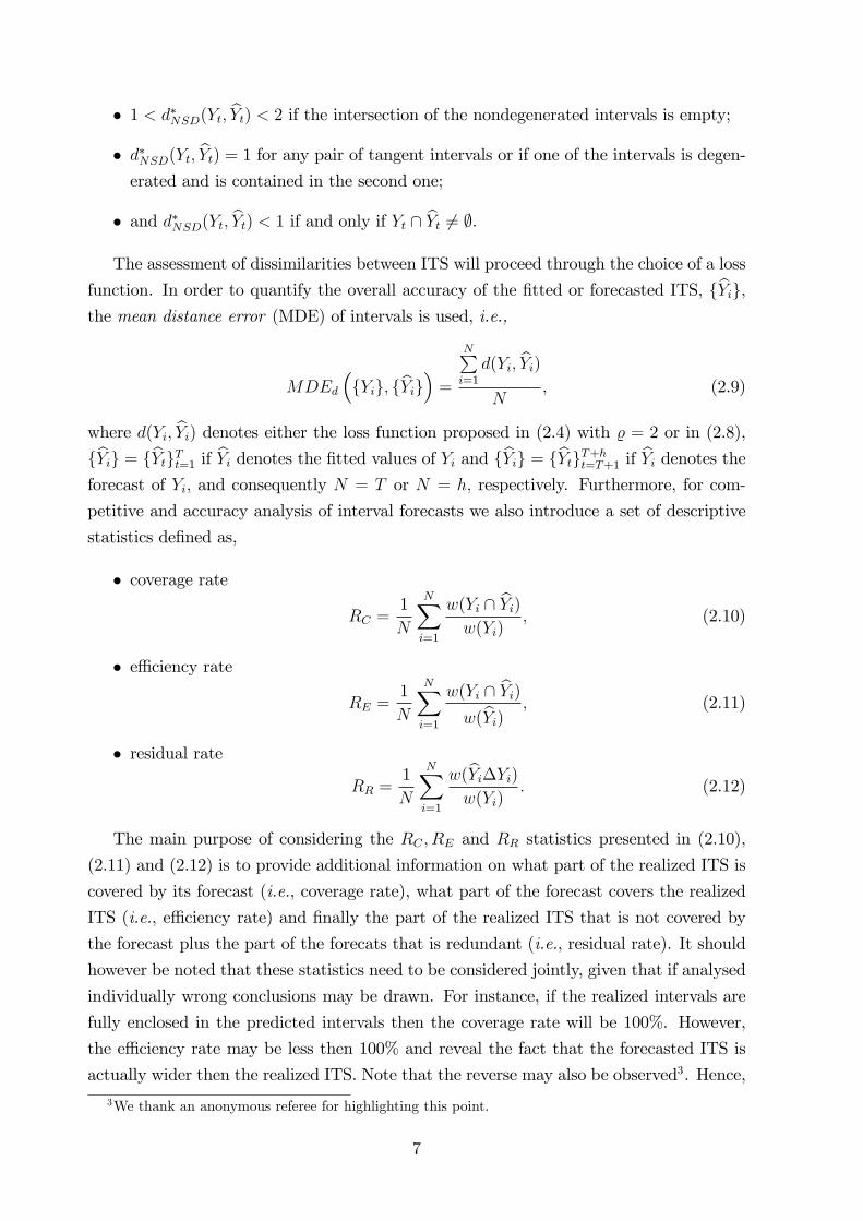
� and d�NSD(Yt; bYt) < 1 if and only if Yt \ bYt 6= ;.The assessment of dissimilarities between ITS will proceed through the choice of a loss

function. In order to quantify the overall accuracy of the �tted or forecasted ITS, fbYig,the mean distance error (MDE) of intervals is used, i.e.,

MDEd

�fYig; fbYig� =

NPi=1

d(Yi; bYi)N

; (2.9)

where d(Yi; bYi) denotes either the loss function proposed in (2.4) with % = 2 or in (2.8),fbYig = fbYtgTt=1 if bYi denotes the �tted values of Yi and fbYig = fbYtgT+ht=T+1 if bYi denotes theforecast of Yi; and consequently N = T or N = h; respectively. Furthermore, for com-

petitive and accuracy analysis of interval forecasts we also introduce a set of descriptive

statistics de�ned as,

� coverage rate

RC =1

N

NXi=1

w(Yi \ bYi)w(Yi)

; (2.10)

� e¢ ciency rate

RE =1

N

NXi=1

w(Yi \ bYi)w(bYi) ; (2.11)

� residual rate

RR =1

N

NXi=1

w(bYi�Yi)w(Yi)

: (2.12)

The main purpose of considering the RC ; RE and RR statistics presented in (2.10),

(2.11) and (2.12) is to provide additional information on what part of the realized ITS is

covered by its forecast (i.e., coverage rate), what part of the forecast covers the realized

ITS (i.e., e¢ ciency rate) and �nally the part of the realized ITS that is not covered by

the forecast plus the part of the forecats that is redundant (i.e., residual rate). It should

however be noted that these statistics need to be considered jointly, given that if analysed

individually wrong conclusions may be drawn. For instance, if the realized intervals are

fully enclosed in the predicted intervals then the coverage rate will be 100%. However,

the e¢ ciency rate may be less then 100% and reveal the fact that the forecasted ITS is

actually wider then the realized ITS. Note that the reverse may also be observed3. Hence,

3We thank an anonymous referee for highlighting this point.

7

only when the coverage and e¢ ciency rates are reasonably high and the di¤erence between

them is small will these provide indication of a good forecast.

Given the results in (2.9), (2.10), (2.11) and (2.12) we are now able to proceed to the

discussion of the estimation of the CR-SETAR model, the ITS forecast methods and their

respective evaluation.

2.3 Estimation of CR-SETAR models

The parameters of interest are �C , �R, and . Since, model (2.3) is nonlinear in parameters

and discontinuous, sequential conditional least squares (see, e.g., Tong, 1990, and Hansen,

1996) is used to obtain the parameter estimates. For any given value of the LS estimates

of �C and �R are respectively,

b�C( ) = TXt=1

XC;t�1( )XC;t�1( )0

!�1 TXt=1

XC;t�1( )ct

!

and b�R( ) = TXt=1

XR;t�1( )XR;t�1( )0

!�1 TXt=1

XR;t�1( )rt

!:

Consequently, the estimated residuals for the center and radius equations, are b"t( ) =ct�XC;t�1( )

0b�C( ) and b�t( ) = rt�XR;t�1( )0b�R( ); respectively, and the corresponding

estimated residual variances b�2C;T ( ) = 1T

PTt=1b"t( )2 and b�2R;T ( ) = 1

T

PTt=1b�t( )2.

Hence, given that typically is unknown, in order to obtain the model parameter

estimates one requires an estimate of this threshold parameter. Considering that is

the value that optimizes the �t of the model, its estimation can be carried out in two

alternative ways:

(i) through the minimization of the sum of squared residuals from both equations in

(2.3), or equivalently, b = argmin 2�

bS2T ( ); (2.13)

where � is the set of all possible thresholds and bS2T ( ) denotes the sum of the

variances b�2C;T ( ) and b�2R;T ( );(ii) through the minimization of the mean distance error introduced in (2.9), i.e.,

b = argmin 2�

MDEd

�fYtgTt=1 ; fbYt( )gTt=1� = argmin

2�MDEd( ) (2.14)

where bYt( ) = hbct( ); brt( )i, bct( ) and brt( ) are the �tted values of (2.3) for a given .

8

Once b is obtained, the slope estimates are b�C = b�C(b ) and b�R = b�R(b ), and the LSresiduals b"t = b"t(b ) and b�t = b�t(b ), with sample variances b�2C;T = b�2C;T (b ) and b�2R;T =b�2R;T (b ).The minimizations in (2.13) and (2.14) can be performed by direct search. Since bS2T ( )

and MDEd( ) depend on through the indicator function Ifzt�d� g, these two functions

are step functions with at most T steps, with steps occurring at distinct values of the

observed threshold variable zt�d. Thus, the minimization problems in (2.13) and (2.14)

can be reduced to searching over values of equalling the distinct values of zt�d in the

sample, i.e., b = argminzt�d2�

bS2T (zt�d); (2.15)

and b = argminzt�d2�

MDEd(zt�d): (2.16)

It is useful to note that estimates of the threshold which allocate a small number

of observations into one regime are undesirable. This possibility can be excluded by

restricting the search in (2.15) and (2.16) to values of such that a minimum number of

observations in each regime is ensured.

3 Interval Time Series Forecasting Methods

Research on ITS forecasting methods has recently received considerable attention in re-

lated literature. This section reviews available procedures and their contributions to ITS

forecasting, and contributes with new methods.

Most of the proposed ITS forecasting methods can be classi�ed into one of three

groups. The �rst group is based on adaptations of smoothing techniques to ITS. For

instance, Arroyo et al. (2011) and Maia and Carvalho (2011) consider adaptations of

exponential smoothing (ES) methods and ES with damped additive trend. The second

group considers nonparametric pattern recognition methods. The most substantial and

in�uential approaches in this group are the k-nearest neighbors (k-NN) and the multi-

layer perceptions (MLP) as representative of arti�cial neural networks (ANN). The former

is introduced by Yakowitch (1987) to classical time series and adapted by Arroyo et al.

(2010) to ITS. For an extensive review of the latter for interval MLP see e.g., Zhang

(1998) and Munoz et al. (2007). The third group focuses on multivariate models for

ITS which are based on classical linear time series approaches such as ARIMA, VAR and

VEC models (see, e.g., Fiess and MacDonald, 2002, Cheung, 2007, Hu and He, 2007, and

Arroyo et al., 2010). Some regression problems are stressed in Billard and Diday (2000,

2003) and Lima and Carvalho (2010).

9

It is however, consensual in the forecasting literature that no single method is superior

in every situation (see, e.g., Chat�eld, 1988, Makridakis, 1989, and Zou and Yang, 2004)

motivating researchers in the ITS context to combine methods from the di¤erent groups

described above (forecast combinations in the conventional time series literature are also

frequently considered, see, for instance, Clemen, 1989 and Diebold and Lopez, 1996, for

overviews). For instance, Zhang (2003) proposes a hybrid approach based on ARIMA

models and MLP, Maia et al. (2008) apply this method to independent series of lower

and upper bounds, and Maia and Carvalho (2011) consider combining Holt�s smoothing

and interval MLP with accuracy measures based on di¤erencing intervals.

The results of these studies reveal several important insights. First, evidence suggests

that approaches that independently forecast the lower and upper bounds of ITS obtained

the lowest rank among the various models analyzed. This conclusion agrees with the

results obtained in He and Hu (2009), Arroyo et al. (2011) and Maia and Carvalho

(2011). Second, multivariate forecasting methods and methods that treat intervals as

a whole using interval arithmetics are reported to have similar properties and perform

globally better than naïve ITS methods. Third, the performance of the models from

the �rst group becomes less e¤ective in terms of interval accuracy if the underlying data

displays nonlinear features. To solve this problem the second group of approaches (ANN

type procedures) was suggested since it has shown interesting potential in classical time

series forecasting applications (see, e.g., Hill et al. 1994, and Bishop, 1995). However, the

reported evidence of ANN adaptations to ITS is still ambiguous. For instance, Maia et al.

(2008) and Maia and Carvalho (2011) present results favoring univariate MLP, ARIMA-

MLP and ES- interval MLP, respectively, whereas Arroyo et al. (2011) reveal that MLP

and ARIMA MLP as well as interval MLP and ES are not superior to other interval

methods. Hence, forecasting nonlinearities in ITS still remains an important issue.

Due to the fact that real world systems are often nonlinear (see, e.g., Granger and

Terasvita, 1993) it is reasonable to develop mechanisms capable of explaining nonlin-

earities and forecast them. In this paper, we focus our attention on forecasting with

the CR-SETAR model introduced in Section 2. It is important to note that for classical

(SE)TAR models, the overall evidence of relative forecasting performance when compared

to traditional linear forecast methods is mixed (see, e.g., Rothman, 1998, Montgomery

et al., 1998, and Clements and Smith, 1997, 2000). Consequently, in order to improve

the properties of the CR-SETAR ITS forecasts we consider combining the CR-SETAR

forecasts with the k-NN method. The combination of these two approaches aims to build

forecasts based on the speci�ed models for ITS and correct these forecasts using the k-NN

mechanism. In what follows we review brie�y the k-NN algorithm, the computation of

one step ahead CR-SETAR forecasts and discuss details of their combination.

10

3.1 k - Nearest Neighbors Method

The k-NN method is used in the literature to forecast ITS. It is a pattern recognition

procedure used to classify objects based on the closest neighbor in the feature space. The

method can be used for conventional time series forecasting (see Yakowitz, 1987) as well

as for ITS forecasting (see Arroyo et al., 2010).

To brie�y review the k-NN method consider the ITS, fYtgTt=1, and the q-dimensionalinterval vector fYtgq = (Yt; Yt�1; :::; Yt�(q�1))

0; where q 2 N is the number of lags and

t = q; :::; T � 1. The k-nearest neighbors of the most recent (feature) interval vectorfYTgq can be found by using the mean distance measure (2.9), i.e.,

MDEd (fYTgq; fYtgq) =

q�1Pi=0

d(YT�i; Yt�i)

q: (3.1)

Once the dissimilarities for each fYtgq, t = q; :::; T � 1, are computed, the k - closestvectors to fYTgq are selected4. Denote these k vectors as fYT1gq; :::; fYTkgq; with Ti < T;

i = 1; :::; k. Hence, to obtain a forecast, a weighted average of the subsequent values,

YT1+1; :::; YTk+1; is considered, i.e.,

bYT+1 = kXi=1

!i � YTi+1; (3.2)

where !i is the weight assigned to neighbor i, with !i � 0 andkPi=1

!i = 1. The weights can

be the same for all neighbors (!i = 1kfor all i) or inversely proportional to the distance

between fYTgq and fYjgq; j = T1; :::; Tk, i.e.,

!i = ikP

m=1

m

;

with i = (MDEd(fYTgq; fYTigq)+ ")�1, where " � 0 is a constant used to avoid divisionby zero when the distance between two sequences is zero.

3.2 The CR-SETAR Forecasts and Forecast Corrections

In this paper, we focus on one step ahead forecasts from the CR-SETAR model. This will

simplify the derivation of the forecasts and the exposition of the correction suggested.

The method provided can however be extended for multi-step ahead forecasting. Exact

analytical solutions to obtain multi-period forecasts using threshold type nonlinear models

4Note that the number, k; of closest vectors to be used can be obtained by minimizing the mean

distance between fYT gq and f �Y kgq, where f �Y kgq =kPi=1

!i � fYTigq:

11

are generally not available (see, e.g., De Gooijer and Kumar, 1992). Often simulation

methods such as Monte Carlo or Bootstrap approaches are employed to construct these

forecasts (see, e.g., Tiao and Tsay, 1994, and Clements and Smith, 1997) and are reported

to perform reasonably well. As an alternative, one may also use the normal forecast error

method proposed by Al-Qassam and Lane (1989) and adapted by De Gooijer and De

Bruin (1997) to forecast SETAR models. Another possibility is an exact method involving

numerical integration based on Chapman-Kolmogorov relations (see, e.g., De Gooijer and

De Bruin, 1997).

The one step ahead forecasts from the CR-SETARmodel, de�ned as bYT+1 � E[YT+1jFT ];where FT = fYtgT1 ; is straightforwardly obtained from (2.3) as,

bYT+1 = < bcT+1; brT+1 >= < E[gC (cT ) + "T+1jFT ]; E[gR (rT ) + uT+1jFT ] > (3.3)

= < gC (cT ) ; gR (rT ) >;

where gC (:) and gR (:) are nonlinear functions that satisfy model (2.3), i.e.,(gC (ct) = XC;t( )

0�C

gR(rt) = XR;t( )0�R

:

As stated above, in empirical applications, SETAR models do frequently not display

suitable forecasting performance, and the same is true for interval valued data. Therefore,

the k-NN corrections of the nonlinear forecasts may prove useful for practical purposes,

due to the fact that di¤erent aspects of the underlying patterns may be additionally

captured and therefore forecasts improved.

Essentially, the idea is to compute the CR-SETAR forecasts as suggested in (3.3) and

to correct them using the k-NN approach. The forecast correction procedure proposed

is similar to the idea of the hybrid system proposed by Zhang (2003). To illustrate the

procedure, let bYT+1 =< bcT+1; brT+1 > and eYT+1 denote the CR-SETAR and corrected

CR-SETAR forecasts, respectively. For the latter, the following principle is used

eYT+1 =< bcT+1 + b"T+1; brT+1 + b�T+1 >; (3.4)

where b"T+1 and b�T+1 are the correction terms. In order to adjust the forecast bYT+1 theterms b"k�NNT+1 and b�k�NNT+1 are computed from the CR-SETAR residuals using k-NN as,8>><>>:

b"k�NNT+1 =kPi=1

!i � b"Ti+1b�k�NNT+1 =

kPi=1

!i � b�Ti+1 :

The time pattern Ti; i = 1; :::; k; necessary to compute these residuals is obtained through

the application of the k-NN method to the �tted valuesnbYtoT

t=1, and the residuals, b"Ti+1

12

and b�Ti+1; computed asb"Ti+1 = cTi+1 � bcTi+1; b�Ti+1 = rTi+1 � brTi+1:In summary, the proposed methodology for CR-SETAR forecast corrections consists of

two steps. First, the CR-SETAR model is estimated to capture the nonlinear behavior of

the underlying ITS, and in the second step, the k-NN method is used to �nd the pattern

of model �t and failure. If the CR-SETAR cannot re�ect some structure of the data,

the residuals will contain information about the model failure and the k-NN method can

be used to exploit this pattern and predict the correction terms necessary to adjust the

CR-SETAR forecasts.

4 An Empirical Example Using The S&P500 index

To illustrate the methods introduced in this paper, in this section we provide an empirical

application to S&P500 index returns. It will be of interest to verify whether the CR-

SETAR model can provide reference values that help detect high-volatility periods (e.g.

this can be important information for investment strategies). Hence, the objective of

this analysis is twofold. One is to illustrate the potential of the CR-SETAR model in

explaining and forecasting ITS and the other to compare the proposed procedures with

other methods available in the literature. This aspect is covered by comparing the one-

step ahead forecasting performance of the k-NN, the CR-SETAR and the corrected CR-

SETAR given in (3.2), (3.3) and (3.4), respectively, with the naive forecast bYT+1 = YT

which is used as a benchmark. Our comparison analysis is based on the accuracy measures

discussed in Section 2.2.

Our sample consists of weekly S&P 500 interval returns observed from January 3,

1997 to November 12, 2010. This sample is divided into two parts: the �rst subsample,

from January 3, 1997 to December 28, 2007 (574 weeks), is used for estimation purposes

and the second subsample, from January 4, 2008 to November 12, 2010 (150 weeks), to

compute the ITS forecasts and analyze their quality. Table 1 presents the chronology of

major events that a¤ected the stock market in the period under analysis. Note that the

forecast period includes the �nancial crises that started in 2008.

[PLEASE INSERT TABLE 1]

Since the objective of this analysis is to analyze the evolution of returns, the starting point

for building our data set is the adequate de�nition of interval returns. In what follows,

two types of interval returns are considered:

(i) The Expanded returns - which consist of intervals that contain all possible di¤er-ences between index price levels that occur in two neighbor trading periods, i.e.

�Y Et = fyt � yt�1 : yt 2 [lt; ut] ^ yt�1 2 [lt�1; ut�1]g; (4.5)

13

where [lt; ut] is an interval of logarithmic prices. Note that, (4.5) satis�es the de�nition

of interval subtraction (see, e.g. Moore, 2009), thus

�Y Et = Yt � Yt�1:

(ii) The Centered returns - which are intervals of returns for the current period basedon the center of the price index levels for the previous period, i.e.

�Y Ct = fyt � yC;t�1 : yt 2 [lt; ut]g; (4.6)

where yC;t�1 is the center of Yt�1. Figure 1 illustrates the di¤erent representations of the

S&P 500 returns in the upper panel and presents the weekly ranges in the lower panel.

Note that the following relation between �Y Et and �Y C

t can be considered. Considering

�Y Et =< cEt ; r

Et > and �Y C

t =< cCt ; rCt >, then intervals of expanded and centered

returns have the same center (i.e., cEt = cCt ) and the radius of the expanded returns is

the aggregation of the contemporaneous and lagged centered returns radius (i.e., rEt =

rCt + rCt�1).

[PLEASE INSERT FIGURE 1]

4.1 The CR-SETAR Model

Due to the relation between the two types of interval returns de�ned in (4.5) and (4.6) in

what follows we will only consider the model for centered returns since for the expanded

returns it will follow along similar lines. Thus,

ct = (�1 +8Pi=1

�1ict�i +8Pj=1

�1jrt�j)� Ifzt�d� g+

(�2 +8Pi=1

�2ict�i +8Pj=1

�2jrt�j)� Ifzt�d> g + "t;(4.7)

rt = (�1 +8Pi=1

'1ict�i +8Pj=1

�1jrt�j)� Ifzt�d� g+

(�2 +8Pi=1

'2ict�i +8Pj=1

�2jrt�j)� Ifzt�d> g + �t;(4.8)

where ct denotes the center of the centered returns interval and rt denotes the radius. For

convenience of notation we drop the index "C" in cCt and rCt ; so that in what follows,

unless otherwise stated, < ct; rt >=< cCt ; rCt >. Note that eight lags of ct and rt where

considered in both equations as this appeared to be the minimum necessary to adequately

describe the short-run dynamics.

In order to analyze the presence of nonlinearities and threshold e¤ects in the S&P500

returns we considered a standard lag of the radius, zt�d = rt�d for 1 � d � 8, as the

14

threshold variable, but we also investigated other potential threshold variable candidates,

such as lags of the centered returns, zt�d = ct�d, and other stationary transformations

of the price levels. In what follows we report only estimation results when zt�d = rt�d

is used as a threshold variable as this provided the best results. The model �t in terms

of the sum of squared residuals, the interval MDE with di¤erent loss functions and the

sum of squared residuals from (4.7) and (4.8) modelled independently are used to select

the adequate estimate of d. Table 2 reports these results. We �nd that the model with

threshold variable zt�1 = rt�1 provides the best adjustment of all models considered.

[PLEASE INSERT TABLE 2]

Hence, setting bd = 1, minimization of (2.13) and (2.14) is used to estimate the thresh-old parameter . The results obtained show that b SSE = 0:0214, b L2 = 0:0207, andb NSD = 0:0210. Asymptotic valid con�dence intervals for b obtained through (2.13) canbe constructed (see, e.g., Hansen, 2000) to verify whether the obtained threshold para-

meter estimates are statistically signi�cant. At the 95% con�dence level the asymptotic

con�dence interval is [0:0204; 0:0215] and contains all threshold estimates, suggesting that

all three methods provide statistically valid results for the S&P500 return�s data used.

Without loss of generality b NSD will be considered for further analysis.The estimate, b NSD = 0:021, indicates that the CR-SETARmodel in (4.7)-(4.8) classi-

�es the sample observations into one of the two regimes depending on wether the S&P500

radius of interval returns has been higher or lower than 0:021 over the previous period

(week). Of the 565 observations in the �tted sample, 137 fall in the high-volatility regime

(rt�1 > 0:021). Heuristically, we can think of this regime as market swings or volatile peri-

ods, since a high range means wider distribution of possible values of returns over trading

periods. Illustration of the regime splitting is presented in the following section jointly

with the forecast splitting. Note that the large historical recession period of the S&P500

("dot com" aftermath) is mostly associated with the high-volatility period observing the

highest peak in March 2000 when the "dot com" bubble burst occurred.

Tables 3 and 4 present the estimation outputs of model (4.7)-(4.8). We report para-

meter estimates, standard errors, absolute parameter changes over regimes, the number

of observations in each regime and the threshold estimates. According to the general-to-

speci�c modelling strategy, insigni�cant regressors were eliminated if the corresponding

heteroskedasticity robust Wald test presented a p-value that exceeded the 10% signi�cance

level in both regimes (see, e.g., Li, 2006). To assess the dynamics of the point estimates

obtained for the autoregressions in both regimes we also employ spectral analysis. Figure

2 plots the spectral density functions corresponding to the autoregressive coe¢ cients from

the two regimes of equation (4.7) in the left panel and equation (4.8) in the right panel.

Regime 1 (rt�1 � b ) of ct has one large peak corresponding to a cycle with a period of 2-315

weeks whereas regime 2 (rt�1 > b ) of ct has two peaks. One corresponding to a cycle witha period of � 1 week and the second corresponding to a business cycle with a 8-9 years

period. The latter result re�ects the recession frequency given in Table 1. For the returns�

radius equation a di¤erent picture is observed. According to this Figure, the radius in

the high volatility regime (rt�1 > b ) picks up the �1-2 weeks cycle and has business cyclefrequency in the low-volatility regime.

[PLEASE INSERT FIGURE 2]

[PLEASE INSERT TABLE 3 AND 4]

4.2 The Relative Performance of CR-SETAR in Forecasting

In this section we analyze the performance of CR-SETAR forecasts and compare results

with those from the naive method (bYT+1 = YT ), the k-NN method and the corrected CR-

SETAR approach. Two ITS forecasts are obtained from each model which correspond to

forecasts of centered and expanded S&P500 returns given in (4.5) and (4.6). The main

quality measure (and the performance ranking) is based on the MDE discussed in Section

2.2. The descriptive statistics given in (2.10), (2.11) and (2.12) are also used to analyze

the relative performance.

[PLEASE INSERT TABLE 5]

Table 5 quanti�es the performance of the forecasts obtained from the di¤erent ap-

proaches. The k-NN method has been implemented with inversely proportional weights,

since this allows us to neglect the e¤ects of insigni�cant neighbors on the forecasts. The

length of the feature interval vector was set equal to eight (i.e., the same length as the

short-run dynamics in the CR-SETAR model). The estimated number of neighbors isbk = 20. To obtain the CR-SETAR forecasts and their corrections we employ the proce-dures discussed in Section 3.2 (in particular (3.3) and (3.4)).

According to both MDE measures (using dL2 and d�NSD), the CR-SETAR model and

the k-NN method show better performance than the naive approach, which is usually hard

to beat in �nancial time series. The results obtained also show that the CR-SETARmodel

and the k-NN approach have nearly identical forecast performance. It is also observed that

the corrected CR-SETAR forecasts are superior to all methods considered in this paper.

This method presents the highest coverage rates, RC ; (62.9% and 81.2% for centered and

expanded returns, respectively) and forecast e¢ ciency rates, RE; (63.46% and 79.57%,

respectively). As previously discussed, the closeness of the results of these two statistics

can be taken as an indicator of the quality of the forecast.

One conclusion that can be drawn from these results is that (as in the conventional

(SE)TAR context) the CR-SETAR model is limited in forecasting. This shortcoming can

16

be caused by the selected forecasting period which contains a lot of uncertainty (e.g., 2008

crisis) and the fact that the underlying nonlinear pattern may not be strong enough in

this period. However, the results in Table 5 indicate that the forecast correction based on

the nonparametric k-NN method can remedy this drawback. Figure 3 shows the regime

splitting for the estimation period (1997-2007) and for the forecast period (2008- 2010).

According to the estimate of most of the high volatility periods (as expected) have been

found during recessions, the "dot-com" aftermath and the 2008 crisis.

[PLEASE INSERT FIGURE 3]

5 Conclusions

This paper develops new methods for the estimation and forecasting of interval-valued

time series. We introduced a threshold-type model for the center-radius representation

of ITS and shown that the model is rather straightforward to estimate using sequen-

tial conditional LS (as in the conventional time series context). We reviewed available

forecasting methods for ITS and introduced new approaches based on the nonparametric

k-NN algorithm and the CR-SETAR model.

The methods are applied to S&P500 index returns for the period from 1997 to 2010.

We �nd that CR-SETAR and k-NN exhibit satisfactory performance in forecasting ITS by

beating the naive method, which is usually hard to outperform in �nancial settings. Thus,

both approaches seem to be useful for forecasting ITS. However, the corrected CR-SETAR

forecasts achieved the best performance based on the proposed accuracy measures. This

is an important result since it shows that CR-SETAR may be limited in the explicit

explanation of the underlying nonlinear pattern but the combination of the two methods

may �nd constructive use in applications. Another important point to highlight from

the results obtained is that the model is potentially useful in the analysis of volatility

dynamics. In particular distinguishing high volatile periods based on the behavior of the

returns�radius.

Several extensions of the methods presented will be pursued in future work. First, it

will be interesting to compare our results with those of other nonlinear models (such as,

e.g., Markov switching models, smooth transition models, and ANN). Second, it will also

be important to investigate how well the radius component of ITS does in forecasting

volatility.

17

References

[1] Al-Qassam, M. S. and J. A. Lane, 1989. Forecasting exponential autoregressive mod-

els of order 1. Journal of Time Series Analysis 10, 95-113.

[2] Alizadeh, S., M.W. Brandt and F.X. Diebold, 2002. Range-based estimation of sto-

chastic volatility models. The Journal of Finance, 53(3), 1047-1091.

[3] Arroyo, J. and C. Mate, 2006. Introducing interval time series: accuracy measures.

In COMPSTAT 2006, Proceeding in Computational statistics, Heidelberg, 1139-1146.

[4] Arroyo, J., R. Espínola and C. Maté, 2011. Di¤erent Approaches to Forecast Interval

Time Series: A Comparison in Finance. Computational Economics. 37: 169-191.

[5] Arroyo, J., G. González-Rivera and C. Maté, 2010. Forecasting with Interval and

Histogram Data. Some Financial Applications. 247-279. Chapter in Handbook of Em-

pirical Economics and Finance. Chapman & Hall/CRC.

[6] Beckers, S., 1983. Variance of Security Price Return Based on High, Low and Closing

Prices. Journal of Business 56, 97-112.

[7] Billard, L. and E. Diday, 2000. Regression analysis for interval-valued data. In Data

Analysis, Classi�cation and Related Methods: Proceedings of the 7th Conference of

the IFCS, IFCS 2002, Berlín, pp. 369�374. Springer.

[8] Billard, L. and E. Diday, 2003. From the Statistics of Data to the Statistics of Knowl-

edge: Symbolic Data Analysis. Journal of the American Statistical Association 98,

470-487.

[9] Bishop, C.M., 1995. Neural networks for pattern recognition. Oxford: Oxford Uni-

versity Press.

[10] Brandt, M. and C. Jones, 2002. Volatility Forecasting with Range-based EGARCH

Models. Manuscript, Wharton School, University of Pennsylvania.

[11] Chat�eld C., 1988. What is the �best�method of forecasting?. Journal of Applied

Statistics 15, 19-39.

[12] Chat�eld C., 1996. Model Uncertainty and Forecast accuracy. Journal of Forecasting

15, 495-508.

[13] Cheung, Y.W., 2007. An Empirical Model of Daily Highs and Lows. International

Journal of Finance and Economics 12, 1-20.

18

[14] Chou, R.Y., 2005. Forecasting Financial Volatilities with Extreme Values: The Con-

ditional Autoregressive Range (CARR) Model. Journal of Money, Credit, and Baking

37(3), 561-582.

[15] Clemen, R.T., (1989) Combining Forecasts: A Review and Annotated Bibliography.

International Journal of Forecasting 5, 559-581.

[16] Clements, M. P. and J. Smith, 1997. The performance of alternative forecasting

methods for SETAR models. International Journal of Forecasting, 13, 463-475.

[17] Clements, M. P. and J. Smith, 1999. A Monte Carlo Study of the Forecasting Perfor-

mance of Empirical SETAR Models, Journal of Applied Econometrics, 14(2), 123-41,

[18] Clements, M. P. and J. Smith, 2000. Evaluating the Forecast densities of linear

and nonlinear models: applications to output growth and unemployment. Journal of

Forecasting 19, 255-276.

[19] De Gooijer, J.G., and K. Kumar, 1992. Some Recent Developments in Non-linear

Time Series Modelling, Testing and Forecasting. International Journal of Forecasting,

8, 135-156.

[20] De Gooijer, J.G., and De Bruin, P.T., 1997. On forecasting SETAR processes. Sta-

tistics and Probability Letters 37, 7�14.

[21] Diebold, F.X. and J.A. Lopez (1996) Forecast Evaluation and Combination, in Mad-

dala and Rao (eds.) Handbook of Statistics, Elsevier, Amsterdam.

[22] Dueker, M., S. Martin and F. Spangnolo, 2007. Contemporaneous Threshold Autore-

gressive Models: Estimation, Testing and Forecasting. Journal of Econometrics 141,

517-547.

[23] Fiessa, N.M. and R. MacDonald, 2002. Towards the fundamentals of technical analy-

sis: analysing the information content of High, Low and Close prices. Economic

Modelling 19, 353-374.

[24] Garcia-Ascanio, C. and C. Mate, 2010. Electric Power Demand Forecasting Using

Interval Time Series: A Comparison between VAR and iMLP. Energy Policy, 38(2),

715-725.

[25] Granger, C.W.J. and T. Terasvirta, 1993. Modelling Nonlinear Economic Relation-

ships. Oxford University Press, Oxford.

[26] Han Ai, Y. Hong, K.K. Lai and S. Wang, 2008. Interval time series analysis with

an application to the sterling-dolar exchange rate. Journal of System Science and

Complexity 21, 558-573.

19

[27] Hansen, B., 1996. Inference when a nuisance parameter is not identi�ed under the

null hypothesis. Econometrica 64, 413-430.

[28] Hansen, B., 2000. Sample splitting and threshold estimation. Econometrica 68, 575-

603.

[29] He, L.T. and C. Hu, 2009. Impacts of Interval Computing on Stock Market Variability

Forecasting. Computational Economics 33, 263-276.

[30] Henry, Ó., N. Olekaln and P.M. Summers, 2001. Exchange Rate Instability: a Thresh-

old Autoregressive Approach. Economic Record 77, 160-166.

[31] Hill, T., Marquez, L., M. O�Connor and W. Remus, 1994. Arti�cial neural network

models for forecasting and decision making. International Journal of Forecasting 10,

5-15.

[32] Hu, C. and L.T. He, 2007. An application of interval methods to stock market fore-

casting. Reliable Computing, 13(5), 423-434.

[33] Hsu, H.L. and B. Wu, 2008. Evaluating Forecasting Performance for Interval Data.

Computers and Mathematics with Application, 56, 2155-2163.

[34] Ichino, M. and H. Yaguchi, 1994. Generalized Minkowski metrics for mixed and

feature-type data analysis. IEEE Trans. on Systems, Man and Cybernetics, 24(1),

698-708.

[35] Li, J. 2006. Testing Granger Causality in the presence of threshold e¤ects. Interna-

tional Journal of Forecasting 22, 771-780.

[36] Lima, N.E.A. and F.d.A.T. de Carvalho, 2010. Constrained linear regression models

for symbolic interval-valued variables. Computational Statistics & Data Analysis 54,

333-347.

[37] Maia, A.L.S. and F.d.A.T. de Carvalho, 2011. Holt�s exponential smoothing and

neural network models for forecasting interval-valued time series. International Jour-

nal of Forecasting 27, 740-759.

[38] Maia, A.L.S. and F.d.A.T. de Carvalho, and T.B. Ludermira, 2008. Forecasting mod-

els for interval-valued time series Neurocomputing 71, 3344-3352.

[39] Makridakis, S., 1989. Why combining works? International Journal of Forecasting

5, 601-603.

20

[40] Montgomery, A.L., V. Zarnowitz, R.S. Tsay and G. C. Tiao, 1998. Forecasting the

U.S. unemployment rate." Journal of the American Statistical Association 93, 478-

493.

[41] Moore, R.E., R.B. Kearfott and M.J. Cloud, 2009. Introduction to interval analysis.

Philadelphia, PA: SIAM Press.

[42] Muñoz S.R., A., C. Maté, J. Arroyo and Á. Sarabia, 2007. iMLP: Applying Multi-

Layer Perceptrons to Interval-Valued Data. Neural Processing Letters 25, 157-169.

[43] Nguyen, H.T. and B. Wu, 2006. Fundamentals of Statistics with Fuzzy Data.

Springer-Verlag, New-York.

[44] Parkinson, M., 1980. The Extreme Value Method for Estimating the Variance of the.

The Journal of Business 53, 61-65.

[45] Potter, S., 1995. A Nonlinear approach to U.S. GNP. Journal of Applied Economet-

rics, 10, 109-125.

[46] Rothman, P., 1998. Forecasting Asymmetric Unemployment Rates. The Review of

Economics and Statistics 80, 164-168.

[47] Tiao, G.C., and Tsay, R.S., 1994. Some Advances in Non-linear and Adaptive Mod-

elling in Time-series. Journal of Forecasting 13, 109-131.

[48] Tong, H., 1990. Non-Linear Time Series: A Dynamic System Approach. New York:

Oxford University Press.

[49] Yakowitz, S., 1987. Nearest-Neighbour Methods for Time Series Analysis. Journal of

Time Series Analysis 8(2), 235-247.

[50] Zellner, A. and J. Tobias, 2000. A Note on Aggregation, Disaggregation and Fore-

casting Performance. Journal of Forecasting 19, 457-469.

[51] Zhang, G., B. E. Patuwo and M. Y. Hu, 1998. Forecasting with arti�cial neural

networks: The state of the art. International Journal of Forecasting 14, 35-62.

[52] Zhang, G., 2003. Time series forecasting using a hybrid ARIMA and neural network

model. Neurocomputing 50, 159-175.

[53] Zou, H. and Y. Yang, 2004. Combining time series models for forecasting. Interna-

tional Journal of Forecasting 20, 69�84.

21

A Appendix

A.1 Interval operations

De�nition A.1 Considering the intervals A = [aL; aU ] and B = [bL; bU ] the following

interval operations can be stated:

1. The intersection of A and B is empty if either aU < bL or bU < aL. Otherwise,

it is de�ne as

A \ B = fz : z 2 A and z 2 Bg = [maxfaL; bLg;minfaU ; bUg]: (A.1)

2. The union of A and B is a set of all ellements that are in A and B, i.e.,

A [ B = fz : z 2 A or z 2 Bg: (A.2)

3. The interval hull of A and B is also an interval since,

A [ B = [minfaL; bLg;maxfaU ; bUg]: (A.3)

4. The symmetric di¤erence of A and B (denoted as A4B) is the set of real valueswhich are in one of the intervals, but not in both. If A\B = 0 then A4B = A [ Belse

A4B = (A [B)=(A \B): (A.4)

5. The width (or diameter) of A is de�ned as

w(A) = aU � aL: (A.5)

Furthermore, the width of the symmetric di¤erence is given as,

w(A4B) =

(w(A [B)� w(A \B)

w(A [ B)

if A \B 6= ;if A \B = ;

: (A.6)

22

TABLES

Table 1: Chronology of Stock Market Events

Date Event

1997-1999 Late 90s. Development of the "dot-com" bubble in the �nancial markets

2000-2002 Bubble burst. �50% loss of its value in a two-year bear market

2003-2007 Sustainable period

2007-2008 Second bear market of the 21st century

2009-2010 Exit from the crisis and return to economic growth

Table 2: Fit of the model (4.7)-(4.8) with zt�d = rt�d

d SSECenter � 103 SSERadius � 103 SSETotal � 103 MDENSD MDEL2

1 0.287797 0.061789 0.349587 0.512242 0.019820

2 0.318009 0.066868 0.384878 0.521692 0.020619

3 0.315095 0.06535 0.380445 0.521945 0.020478

4 0.313835 0.064676 0.378511 0.526834 0.020793

5 0.311634 0.060816 0.372449 0.526995 0.020663

6 0.316956 0.065794 0.38275 0.522063 0.020599

7 0.316377 0.066105 0.382482 0.530048 0.020852

8 0.322871 0.067857 0.390728 0.530630 0.020842

Table 3: Estimation Results for the Center Model in (4.8)Regime 1 Regime 2 Absolute Change

Coe¤. SE � 102 Coe¤. SE � 102 Wald test over regimes

Constant -0.001 0.001 -0.025 0.003 11.631 (0.003) 0.024

rt�1 0.135 5.397 0.710 2.077 7.621 (0.022) 0.575

rt�2 -0.378 1.198 0.802 3.643 20.756 (0.000) 1.180

rt�4 0.274 2.455 -0.387 1.252 14.023 (0.001) 0.661

rt�5 0.285 2.188 0.191 1.920 7.052 (0.029) 0.094

rt�6 -0.201 1.944 -0.320 1.821 6.436 (0.040) 0.119

ct�1 0.149 0.418 0.213 0.395 7.704 (0.021) 0.064

ct�5 0.089 0.321 0.145 0.562 4.816 (0.090) 0.056

0.021

N 428 137Note: Regime 1 is speci�ed as Rt�1 � 0:021 and Regime 2 as Rt�1 > 0:021.

23

Table 4: Estimation Results for the Radius Model in (4.9)

Regime 1 Regime 2 Absolute Change

Coe¤. SE ��103 Coe¤. SE ��103 Wald test over regimes

Constant 0.005 0.001 0.014 0.01 87.813 (0.000) 0.009

rt�2 0.188 3.04 -0.040 9.09 28.159 (0.000) 0.228

rt�3 0.259 5.32 0.290 4.39 35.539 (0.000) 0.031

rt�6 0.068 4.05 0.123 4.24 6.512 (0.039) 0.055

rt�7 0.125 4.16 -0.034 3.27 8.005 (0.018) 0.159

rt�8 0.077 2.28 0.054 7.35 3.500 (0.174) 0.023

ct�1 -0.106 0.85 -0.082 0.72 22.219 (0.000) 0.024

ct�2 -0.075 0.79 -0.021 1.22 12.985 (0.002) 0.054

ct�3 -0.062 0.73 -0.016 0.92 14.091 (0.001) 0.046

ct�4 0.007 0.71 -0.077 0.76 6.352 (0.042) 0.084

ct�5 0.004 0.63 -0.120 1.02 5.224 (0.073) 0.124

ct�8 0.016 0.61 -0.082 1.06 5.290 (0.071) 0.098

0.021

N 428 137Note: Regime 1 is speci�ed as Rt�1 � 0:021 and Regime 2 as Rt�1 > 0:021.

24

Table5:Competitiveanalysisofthemodelforecastperformance(2008-2010)

CR-SETAR

K-NN

CR-SETARcorrected

Naive

MDE/ForecastCentered

Expanded

Centered

Expanded

Centered

Expanded

Centered

Expanded

MDEdL2

0.03330

0.03765

0.03278

0.03924

0.02923

0.03261

0.04067

0.04142

MDEd� NSD

0.55388

0.35952

0.55140

0.37130

0.50572

0.32233

0.62360

0.38772

E¢ciencyrate

58.31%

76.99%

59.93%

78.75%

63.46%

79.57%

52.50%

75.10%

Coveragerate

59.75%

79.51%

59.91%

77.32%

62.91%

81.19%

51.56%

74.85%

Residualrate

55.48%

37.88%

54.64%

37.00%

50.29%

32.23%

61,62%

38.77%

25

FIGURES

Figure 1: Lower-upper limits of expanded and centered returns.

Interval Returns

­0.38

­0.28

­0.18

­0.08

0.02

0.12

0.22

0.32

1997 1998 1999 2000 2001 2002 2003 2004 2005 2006 2007 2008 2009 2010

Expanded Returns Centered Returns

0

0.02

0.04

0.06

0.08

0.1

0.12

0.14

0.16

1997 1998 1999 2000 2001 2002 2003 2004 2005 2006 2007 2008 2009 2010

Radius

Figure 2: Spectral Density by Regime for ct and rt

0

0.0002

0.0004

0.0006

0.0008

0.001

0 50 100 150 200 250 300 350 400 450 500 550

Regime 1

Regime 2

0

0.0002

0.0004

0.0006

0.0008

0.001

0 50 100 150 200 250 300 350 400 450 500 550

Regime 1

Regime 2

26

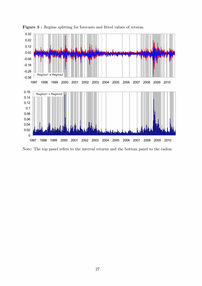
Figure 3 : Regime splitting for forecasts and �tted values of returns.

­0.38

­0.28

­0.18

­0.08

0.02

0.12

0.22

0.32

1997 1998 1999 2000 2001 2002 2003 2004 2005 2006 2007 2008 2009 2010

Regime1 Regime2

00.020.040.060.080.1

0.120.140.16

1997 1998 1999 2000 2001 2002 2003 2004 2005 2006 2007 2008 2009 2010

Regime1 Regime2

Note: The top panel refers to the interval returns and the bottom panel to the radius.

27

Banco de Portugal | Working Papers i

WORKING PAPERS

2010

1/10 MEASURING COMOVEMENT IN THE TIME-FREQUENCY SPACE

— António Rua

2/10 EXPORTS, IMPORTS AND WAGES: EVIDENCE FROM MATCHED FIRM-WORKER-PRODUCT PANELS

— Pedro S. Martins, Luca David Opromolla

3/10 NONSTATIONARY EXTREMES AND THE US BUSINESS CYCLE

— Miguel de Carvalho, K. Feridun Turkman, António Rua

4/10 EXPECTATIONS-DRIVEN CYCLES IN THE HOUSING MARKET

— Luisa Lambertini, Caterina Mendicino, Maria Teresa Punzi

5/10 COUNTERFACTUAL ANALYSIS OF BANK MERGERS

— Pedro P. Barros, Diana Bonfi m, Moshe Kim, Nuno C. Martins

6/10 THE EAGLE. A MODEL FOR POLICY ANALYSIS OF MACROECONOMIC INTERDEPENDENCE IN THE EURO AREA

— S. Gomes, P. Jacquinot, M. Pisani

7/10 A WAVELET APPROACH FOR FACTOR-AUGMENTED FORECASTING

— António Rua

8/10 EXTREMAL DEPENDENCE IN INTERNATIONAL OUTPUT GROWTH: TALES FROM THE TAILS

— Miguel de Carvalho, António Rua

9/10 TRACKING THE US BUSINESS CYCLE WITH A SINGULAR SPECTRUM ANALYSIS

— Miguel de Carvalho, Paulo C. Rodrigues, António Rua

10/10 A MULTIPLE CRITERIA FRAMEWORK TO EVALUATE BANK BRANCH POTENTIAL ATTRACTIVENESS

— Fernando A. F. Ferreira, Ronald W. Spahr, Sérgio P. Santos, Paulo M. M. Rodrigues

11/10 THE EFFECTS OF ADDITIVE OUTLIERS AND MEASUREMENT ERRORS WHEN TESTING FOR STRUCTURAL BREAKS

IN VARIANCE

— Paulo M. M. Rodrigues, Antonio Rubia

12/10 CALENDAR EFFECTS IN DAILY ATM WITHDRAWALS

— Paulo Soares Esteves, Paulo M. M. Rodrigues

13/10 MARGINAL DISTRIBUTIONS OF RANDOM VECTORS GENERATED BY AFFINE TRANSFORMATIONS OF

INDEPENDENT TWO-PIECE NORMAL VARIABLES

— Maximiano Pinheiro

14/10 MONETARY POLICY EFFECTS: EVIDENCE FROM THE PORTUGUESE FLOW OF FUNDS

— Isabel Marques Gameiro, João Sousa

15/10 SHORT AND LONG INTEREST RATE TARGETS

— Bernardino Adão, Isabel Correia, Pedro Teles

16/10 FISCAL STIMULUS IN A SMALL EURO AREA ECONOMY

— Vanda Almeida, Gabriela Castro, Ricardo Mourinho Félix, José Francisco Maria

17/10 FISCAL INSTITUTIONS AND PUBLIC SPENDING VOLATILITY IN EUROPE

— Bruno Albuquerque

Banco de Portugal | Working Papers ii

18/10 GLOBAL POLICY AT THE ZERO LOWER BOUND IN A LARGE-SCALE DSGE MODEL

— S. Gomes, P. Jacquinot, R. Mestre, J. Sousa

19/10 LABOR IMMOBILITY AND THE TRANSMISSION MECHANISM OF MONETARY POLICY IN A MONETARY UNION

— Bernardino Adão, Isabel Correia

20/10 TAXATION AND GLOBALIZATION

— Isabel Correia

21/10 TIME-VARYING FISCAL POLICY IN THE U.S.

— Manuel Coutinho Pereira, Artur Silva Lopes

22/10 DETERMINANTS OF SOVEREIGN BOND YIELD SPREADS IN THE EURO AREA IN THE CONTEXT OF THE ECONOMIC

AND FINANCIAL CRISIS

— Luciana Barbosa, Sónia Costa

23/10 FISCAL STIMULUS AND EXIT STRATEGIES IN A SMALL EURO AREA ECONOMY

— Vanda Almeida, Gabriela Castro, Ricardo Mourinho Félix, José Francisco Maria

24/10 FORECASTING INFLATION (AND THE BUSINESS CYCLE?) WITH MONETARY AGGREGATES

— João Valle e Azevedo, Ana Pereira

25/10 THE SOURCES OF WAGE VARIATION: AN ANALYSIS USING MATCHED EMPLOYER-EMPLOYEE DATA

— Sónia Torres,Pedro Portugal, John T.Addison, Paulo Guimarães

26/10 THE RESERVATION WAGE UNEMPLOYMENT DURATION NEXUS

— John T. Addison, José A. F. Machado, Pedro Portugal

27/10 BORROWING PATTERNS, BANKRUPTCY AND VOLUNTARY LIQUIDATION

— José Mata, António Antunes, Pedro Portugal

28/10 THE INSTABILITY OF JOINT VENTURES: LEARNING FROM OTHERS OR LEARNING TO WORK WITH OTHERS

— José Mata, Pedro Portugal

29/10 THE HIDDEN SIDE OF TEMPORARY EMPLOYMENT: FIXED-TERM CONTRACTS AS A SCREENING DEVICE

— Pedro Portugal, José Varejão

30/10 TESTING FOR PERSISTENCE CHANGE IN FRACTIONALLY INTEGRATED MODELS: AN APPLICATION TO WORLD

INFLATION RATES

— Luis F. Martins, Paulo M. M. Rodrigues

31/10 EMPLOYMENT AND WAGES OF IMMIGRANTS IN PORTUGAL

— Sónia Cabral, Cláudia Duarte

32/10 EVALUATING THE STRENGTH OF IDENTIFICATION IN DSGE MODELS. AN A PRIORI APPROACH

— Nikolay Iskrev

33/10 JOBLESSNESS

— José A. F. Machado, Pedro Portugal, Pedro S. Raposo

2011

1/11 WHAT HAPPENS AFTER DEFAULT? STYLIZED FACTS ON ACCESS TO CREDIT

— Diana Bonfi m, Daniel A. Dias, Christine Richmond

2/11 IS THE WORLD SPINNING FASTER? ASSESSING THE DYNAMICS OF EXPORT SPECIALIZATION

— João Amador

Banco de Portugal | Working Papers iii

3/11 UNCONVENTIONAL FISCAL POLICY AT THE ZERO BOUND

— Isabel Correia, Emmanuel Farhi, Juan Pablo Nicolini, Pedro Teles

4/11 MANAGERS’ MOBILITY, TRADE STATUS, AND WAGES

— Giordano Mion, Luca David Opromolla

5/11 FISCAL CONSOLIDATION IN A SMALL EURO AREA ECONOMY

— Vanda Almeida, Gabriela Castro, Ricardo Mourinho Félix, José Francisco Maria

6/11 CHOOSING BETWEEN TIME AND STATE DEPENDENCE: MICRO EVIDENCE ON FIRMS’ PRICE-REVIEWING

STRATEGIES

— Daniel A. Dias, Carlos Robalo Marques, Fernando Martins

7/11 WHY ARE SOME PRICES STICKIER THAN OTHERS? FIRM-DATA EVIDENCE ON PRICE ADJUSTMENT LAGS

— Daniel A. Dias, Carlos Robalo Marques, Fernando Martins, J. M. C. Santos Silva

8/11 LEANING AGAINST BOOM-BUST CYCLES IN CREDIT AND HOUSING PRICES

— Luisa Lambertini, Caterina Mendicino, Maria Teresa Punzi

9/11 PRICE AND WAGE SETTING IN PORTUGAL LEARNING BY ASKING

— Fernando Martins

10/11 ENERGY CONTENT IN MANUFACTURING EXPORTS: A CROSS-COUNTRY ANALYSIS

— João Amador

11/11 ASSESSING MONETARY POLICY IN THE EURO AREA: A FACTOR-AUGMENTED VAR APPROACH

— Rita Soares

12/11 DETERMINANTS OF THE EONIA SPREAD AND THE FINANCIAL CRISIS

— Carla Soares, Paulo M. M. Rodrigues

13/11 STRUCTURAL REFORMS AND MACROECONOMIC PERFORMANCE IN THE EURO AREA COUNTRIES: A MODEL-

BASED ASSESSMENT

— S. Gomes, P. Jacquinot, M. Mohr, M. Pisani

14/11 RATIONAL VS. PROFESSIONAL FORECASTS

— João Valle e Azevedo, João Tovar Jalles

15/11 ON THE AMPLIFICATION ROLE OF COLLATERAL CONSTRAINTS

— Caterina Mendicino

16/11 MOMENT CONDITIONS MODEL AVERAGING WITH AN APPLICATION TO A FORWARD-LOOKING MONETARY

POLICY REACTION FUNCTION

— Luis F. Martins

17/11 BANKS’ CORPORATE CONTROL AND RELATIONSHIP LENDING: EVIDENCE FROM RETAIL LOANS

— Paula Antão, Miguel A. Ferreira, Ana Lacerda

18/11 MONEY IS AN EXPERIENCE GOOD: COMPETITION AND TRUST IN THE PRIVATE PROVISION OF MONEY

— Ramon Marimon, Juan Pablo Nicolini, Pedro Teles

19/11 ASSET RETURNS UNDER MODEL UNCERTAINTY: EVIDENCE FROM THE EURO AREA, THE U.K. AND THE U.S.

— João Sousa, Ricardo M. Sousa

20/11 INTERNATIONAL ORGANISATIONS’ VS. PRIVATE ANALYSTS’ FORECASTS: AN EVALUATION

— Ildeberta Abreu

21/11 HOUSING MARKET DYNAMICS: ANY NEWS?

— Sandra Gomes, Caterina Mendicino

Banco de Portugal | Working Papers iv

22/11 MONEY GROWTH AND INFLATION IN THE EURO AREA: A TIME-FREQUENCY VIEW

— António Rua

23/11 WHY EX(IM)PORTERS PAY MORE: EVIDENCE FROM MATCHED FIRM-WORKER PANELS

— Pedro S. Martins, Luca David Opromolla

24/11 THE IMPACT OF PERSISTENT CYCLES ON ZERO FREQUENCY UNIT ROOT TESTS

— Tomás del Barrio Castro, Paulo M.M. Rodrigues, A.M. Robert Taylor

25/11 THE TIP OF THE ICEBERG: A QUANTITATIVE FRAMEWORK FOR ESTIMATING TRADE COSTS

— Alfonso Irarrazabal, Andreas Moxnes, Luca David Opromolla

26/11 A CLASS OF ROBUST TESTS IN AUGMENTED PREDICTIVE REGRESSIONS

— Paulo M.M. Rodrigues, Antonio Rubia

27/11 THE PRICE ELASTICITY OF EXTERNAL DEMAND: HOW DOES PORTUGAL COMPARE WITH OTHER EURO AREA

COUNTRIES?

— Sónia Cabral, Cristina Manteu

28/11 MODELING AND FORECASTING INTERVAL TIME SERIES WITH THRESHOLD MODELS: AN APPLICATION TO

S&P500 INDEX RETURNS

— Paulo M. M. Rodrigues, Nazarii Salish