modeling and control of a four-axis control moment gyroscope · may 2013. aknowledgement ... 2.3...
TRANSCRIPT
CZECH TECHNICAL UNIVERSITY IN PRAGUE
Faculty of Electrical Engineering
Department of Control Engineering
Modeling and control
of a four-axis control moment gyroscope
Bachelor Thesis
Author: Evyatar Bukai
Tutor: Ing. Zdenek Hurak, Ph.D.
May 2013


Aknowledgement
Foremost, I would like to thank Ing. Zdenek Hurak, Ph.D. for leading me through-
out this project and being a helpful and knowledgeable tutor without whose guidance I would
not be able to complete this work. I would also like to thank the team AA4CC, part of the Con-
trol Department, for being accessible and contributive for the knowledge acquired throughout
the project.

Abstract
In this thesis we describe the dynamical model and define control algorithms for the four-
axis control moment gyroscope. The educational laboratory experimental platform, product
of Educational Control Products (ECP), is modeled following two approaches: The analytical
approach is led through Lagrangian method, whereas the numerical approach is done with the
use of SimMechanics. After identification of the physical parameters, the resulting analytical
model is compared with the measured responses obtained from experimental measurements. A
short discussion of control design issues is proposed. Finally, the reader will be able to exploit
the system following the hints given throughout the thesis.

Contents
List of Figures xi
List of Tables xiii
1 Motivation and goals 1
2 Mathematical modeling of the four-axis control moment gyroscope 3
2.1 System overview . . . . . . . . . . . . . . . . . . . . . . . . . . . . . . . . . . . 3
2.1.1 Coordinate frame . . . . . . . . . . . . . . . . . . . . . . . . . . . . . . . 4
2.1.2 System inputs . . . . . . . . . . . . . . . . . . . . . . . . . . . . . . . . . 5
2.1.3 Inertias . . . . . . . . . . . . . . . . . . . . . . . . . . . . . . . . . . . . 5
2.1.4 Kinematics . . . . . . . . . . . . . . . . . . . . . . . . . . . . . . . . . . 6
2.2 Nonlinear dynamical model . . . . . . . . . . . . . . . . . . . . . . . . . . . . . 7
2.2.1 Kinetic energy of the system . . . . . . . . . . . . . . . . . . . . . . . . 7
2.2.2 Lagrangian of the dynamical system . . . . . . . . . . . . . . . . . . . . 9
2.3 Linear dynamical model . . . . . . . . . . . . . . . . . . . . . . . . . . . . . . . 9
2.3.1 Linearized model about the selected operating points . . . . . . . . . . . 9
2.3.2 Linearized equations for constrained models . . . . . . . . . . . . . . . . 10
2.4 Computer aided design (CAD) modeling . . . . . . . . . . . . . . . . . . . . . . 12
2.4.1 The mechanical system under SimMechanics . . . . . . . . . . . . . . . 14
3 Laboratory experiments 17
3.1 Software and hardware setup . . . . . . . . . . . . . . . . . . . . . . . . . . . . 17
3.1.1 ECP Executive software overview . . . . . . . . . . . . . . . . . . . . . . 17
3.1.2 Hardware installation and operation . . . . . . . . . . . . . . . . . . . . 20
3.2 Experiments for determining the physical parameters of the system . . . . . . . 23
3.2.1 Measurement of inertias . . . . . . . . . . . . . . . . . . . . . . . . . . . 23
3.2.2 Measurement of the control effort gains . . . . . . . . . . . . . . . . . . 27
3.2.3 Measurement of the encoder gains . . . . . . . . . . . . . . . . . . . . . 30
3.2.4 Measurement of the friction acting on the rotor disk . . . . . . . . . . . 31
3.3 Verification of the mathematical model . . . . . . . . . . . . . . . . . . . . . . . 33
3.3.1 For all gimbals free of motion . . . . . . . . . . . . . . . . . . . . . . . . 33
3.3.2 For all gimbals free of motion except Gimbal #2 . . . . . . . . . . . . . 35
3.3.3 For all gimbals free of motion except Gimbal #3 . . . . . . . . . . . . . 36
4 Feedback control 39
4.1 Setting a feedback control in the ECP environment . . . . . . . . . . . . . . . . 39
ix

x
4.1.1 Structuring the Control Algorithm . . . . . . . . . . . . . . . . . . . . . 40
4.1.2 Control Algorithm under the ECP Executive program . . . . . . . . . . 43
4.2 Controlling the positions of body C and D using Cascade control . . . . . . . . 48
5 Conclusion 53
Bibliography 55
A CD content 57
List of Figures
1.1 ECP Model 750 - The control moment gyroscope . . . . . . . . . . . . . . . . . 2
2.1 System overview : Coordinate frame definition . . . . . . . . . . . . . . . . . . 4
2.2 Autodesk Inventor Professional CAD : Software overview . . . . . . . . . . . . 12
2.3 Autodesk Inventor Professional CAD : modeling the four-axis control momentgyroscope . . . . . . . . . . . . . . . . . . . . . . . . . . . . . . . . . . . . . . . 13
2.4 SimMechanics model of our system . . . . . . . . . . . . . . . . . . . . . . . . . 14
2.5 Angular velocity of body C given sinusoidal input . . . . . . . . . . . . . . . . . 15
2.6 Block diagram of the dynamical system under SimMechanics . . . . . . . . . . 15
3.1 ECP background screen display . . . . . . . . . . . . . . . . . . . . . . . . . . . 18
3.2 Overview of the real-time control system . . . . . . . . . . . . . . . . . . . . . . 21
3.3 Mechanism drive block diagram . . . . . . . . . . . . . . . . . . . . . . . . . . . 22
3.4 Configuration of the system for the selected moments of inertias experiments . 23
3.5 Data for JC measurement . . . . . . . . . . . . . . . . . . . . . . . . . . . . . . 24
3.6 Data for KA measurement . . . . . . . . . . . . . . . . . . . . . . . . . . . . . . 26
3.7 Data for IC measurement . . . . . . . . . . . . . . . . . . . . . . . . . . . . . . 27
3.8 Configuration of the system for the control effort gain tests . . . . . . . . . . . 28
3.9 Data for ku1 measurement . . . . . . . . . . . . . . . . . . . . . . . . . . . . . . 29
3.10 Data for ku2 measurement . . . . . . . . . . . . . . . . . . . . . . . . . . . . . . 30
3.11 Measurement of Encoder 1 Velocity given a maximum control effort step input 32
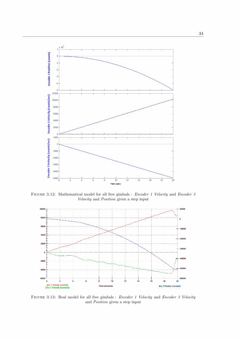
3.12 Mathematical model for all free gimbals : Encoder 1 Velocity and Encoder 3Velocity and Position given a step input . . . . . . . . . . . . . . . . . . . . . . 34
3.13 Real model for all free gimbals : Encoder 1 Velocity and Encoder 3 Velocity andPosition given a step input . . . . . . . . . . . . . . . . . . . . . . . . . . . . . 34
3.14 Comparison of real model and mathematical model of Encoder 3 Position givena step input . . . . . . . . . . . . . . . . . . . . . . . . . . . . . . . . . . . . . . 35
3.15 Mathematical model for Gimbal #3 Locked : Encoder 2 Velocity and Encoder4 Velocity given sinusoidal input . . . . . . . . . . . . . . . . . . . . . . . . . . 36
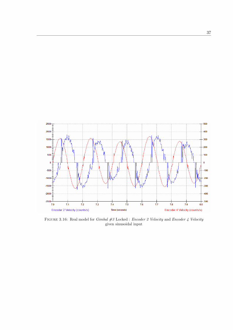
3.16 Real model for Gimbal #3 Locked : Encoder 2 Velocity and Encoder 4 Velocitygiven sinusoidal input . . . . . . . . . . . . . . . . . . . . . . . . . . . . . . . . 37
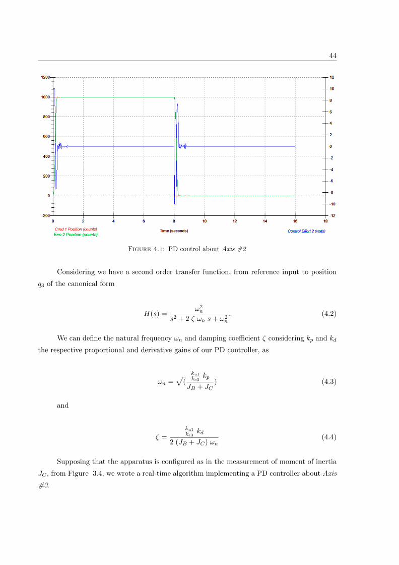
4.1 PD control about Axis #2 . . . . . . . . . . . . . . . . . . . . . . . . . . . . . . 44
4.2 Oscillating system responses for different values of kP . . . . . . . . . . . . . . 45
4.3 PD control about Axis #3 with kP = 8.2 and different values of kD . . . . . . 46
4.4 Control using the proportional and derivative gains as in the critically dampedcase with integral gain ki = 17 . . . . . . . . . . . . . . . . . . . . . . . . . . . 47
4.5 Successive loop closure control diagram . . . . . . . . . . . . . . . . . . . . . . 47
xi
xii
4.6 Gyroscopic torque control using successive loop closure and PD for differentinput step trajectory . . . . . . . . . . . . . . . . . . . . . . . . . . . . . . . . . 49
4.7 Gyroscopic torque control using successive loop closure and PD for input ramptrajectory . . . . . . . . . . . . . . . . . . . . . . . . . . . . . . . . . . . . . . . 50
4.8 Anti-windup effect on the PID controller with respect to the set current satu-ration of Motor #1 . . . . . . . . . . . . . . . . . . . . . . . . . . . . . . . . . . 51
4.9 Position control using cascade control . . . . . . . . . . . . . . . . . . . . . . . 51
4.10 Position control of body D using cascade control . . . . . . . . . . . . . . . . . 52
4.11 Position control of body C using cascade control . . . . . . . . . . . . . . . . . 52

List of Tables
3.1 Encoder gains . . . . . . . . . . . . . . . . . . . . . . . . . . . . . . . . . . . . . 31
3.2 Moments of inertia . . . . . . . . . . . . . . . . . . . . . . . . . . . . . . . . . . 31
3.3 Control effort gains . . . . . . . . . . . . . . . . . . . . . . . . . . . . . . . . . . 31
4.1 Functions available through the ECP Executive editor . . . . . . . . . . . . . . 41
4.2 Comparators available through the ECP Executive editor . . . . . . . . . . . . 42
4.3 Motors specifications . . . . . . . . . . . . . . . . . . . . . . . . . . . . . . . . . 49
xiii

xv
Abbreviations
DSP Digital Signal Processor
PID/PD Generic control loop feedback mechanism used in industrial controlsystems. It involves three separate constant parameters: the propo--rtional (P), integral (I) and derivative (D) values.
DAC Digital-to-Analog converter.
RPM Revolutions per minute.
ECP Educational Control Products company.
CMG The control moment gyroscope.
Symbols
qi Angular position about the axis of rotation of the ith (i=A,B,C,D)body [rad or counts].
ωi Angular velocity about the axis of rotation of the ith (i=A,B,C,D)body [rad/sec or counts/sec].
Ii, Ji,Ki Scalar moments of inertia about the orthogonal unit vectors of theith (i=A,B,C,D) body [kg · m2].
T1, T2 Torque applied to body D by body C and torque applied to body Cby body B respectively [N · m].
Ω Spin speed of the rotor disk (D) [RPM].
kei Encoder gain of the ith (i=1,2,3,4) encoder [counts/rad].
kui Control effort gain of the ith (i=1,2) plant input [N/count].


Chapter 1
Motivation and goals
The control moment gyroscope is nowadays highly used in control of the orientation
of spacecraft devices with respect to an inertial frame, also called attitude control. Indeed,
rotating a spacecraft can be achieved in different ways.
Classical means for its rotation, as the use of thrusters - propulsive devices for sta-
tion keeping and attitude control in the reaction control system, are energy consuming and
expensive to operate.
The resulted gyroscope torque of the control moment gyroscope, obtained via actuation
of its gimbals via electric motors, provides a three-axis rotation of the spacecraft using only
electrical power, such as solar power. This is a low cost and very efficient maneuver, resulting
in an action that can be done on regular basis. In opposite to the reaction wheel, the instan-
taneous torque available through the control moment gyroscope is not limited by the motor
itself, which leads to great effects for international space stations, satellites, as well as Hubble
space telescopes. A few hundred watts and a mass of a hundred of kilograms can produce a
couple of thousands of newton meters of torque.
The main objective of my thesis is to study and enrich the usage of Educational Control
Products’ four axis control moment gyroscope system, for teaching purpose and better under-
standing of modeling, simulation and control of similar highly non-linear multibody systems.
The study of the system will be done in three distinct phases. In the second chapter we will
build the dynamical model of the system using two approaches: An analytical course, using
Lagrangian method, and a numerical way, using object-oriented modeling. In Chapter 3, we
will verify the mathematical model using laboratory experiments, identify the physical param-
eters of the system and acquire software routines for exporting and importing measured data
to and from Matlab. Finally, in Chapter 4, we will demonstrate basic control design techniques
for control assignments with the provided experimental setup.
1

2
Figure 1.1: ECP Model 750 - The control moment gyroscope

Chapter 2
Mathematical modeling of the
four-axis control moment gyroscope
The four-axis control moment gyroscope can be set into a range of dynamical configura-
tions. Its behavior, highly nonlinear in its global workspace, could be simplified and linearized
with the use of constraints available through the appliance of its electromechanical brakes.
This chapter deals with the configuration and equations of motion describing the system, in
its global workspace and for some special cases, suitable for the analysis and control design of
the system.
2.1 System overview
The ECP model 750 Control Moment Gyroscope consists of an electromechanical plant,
in addition to the control software and hardware described and analyzed throughout Chapter 3.
The use of constraints and input torques, applied by direct-acting or reaction, allows the user
to obtain a range of dynamical configurations, resulting in a system ranging from one to four
degrees of freedom and four angular outputs. The dynamical system could develop in a linear
or highly non-linear behavior, in its full capacity to operate. The one or two applied input high
torque density, of rare earth magnet type DC servo motors, can be applied simultaneously if
required and offer a possibility for control effort transmission.
In addition to the input torques, the system offers high resolution encoders for angle
feedback, as well as low friction slip rings for motor power and signal across the gimbals.
The safety shutdown and the electromechanical brakes, as well as the inertial switched for
high gimbals speed detection, ease the change of dynamical configurations of the system while
offering safety shutdown.
3

4
Furthermore to the electromechanical plant, the system consists of a real-time controller
unit and of the software provided by the manufacturer.
Along with the servo amplifiers, the power supplies and the actuator interfaces, the real-
time controller unit includes a Digital Signal Processor (DSP), executing control laws at high
sampling rates. This offers the possibility to the modeled implementation to be discrete or
continuous in time. The controller offers data acquisition and trajectory generation, whereas
two auxiliary digital-to-analog converters provide real-time analog signal measurement.
Finally, the software provided by the manufacturer, the ECP Executive program, offers
the user’s interface to the system. It describes the data acquisition, the plotting, the execution
commands, the trajectory definition and the controller specification provided by the system’s
own language, supporting basic or highly complex algorithms, implemented by the DSP via
an auto-compiler within the software.
2.1.1 Coordinate frame
Figure 2.1: System overview : Coordinate frame definition
From Figure 2.1, the four degrees of freedom plant is formed by the outer gimbal (body
A), the inner gimbal (body B), the rotor drum (body C) and the rotor disk (body D). The
orthogonal unit vectors ri (i=1,2,3) are fixed in the inertial reference frame. Auxiliary, the
orthogonal unit vectors ai, bi, ci and di (i=1,2,3) are fixed in bodies A, B, C and D respectively.

5
2.1.2 System inputs
The two considered inputs of the system are the torques T1 and T2, applied respectively
via Motor #1 and Motor #2. T1 is applied by body C to body D via the rotor spin motor,
resulting in torques acting on the two bodies, which can be described by Equations 2.1 and
2.2. T2 is applied by body B to body C via the gimbal motor, resulting into torques acting on
these two bodies, which can be described by Equations 2.3 and 2.4 .
TD = T1d2 (2.1)
TC = −T1d2 (2.2)
TC = T2c1 (2.3)
TB = −T2c1 (2.4)
2.1.3 Inertias
For analytical purposes, we assumed that the mass center of all the bodies of the system
are at the center of the rotor disk, body D. This attests that we can neglect gravity and take
into consideration only the rotational dynamics. With each matrix given in the coordinate
frame of the respective body, we can define its diagonal inertia matrix. Establishing Ix, Jx
and Kx the scalar moments of inertia of each body (x= A,B,C,D) about the ith (i= 1,2,3)
direction, we can write
IA =
∣∣∣∣∣∣∣∣IA 0 0
0 JA 0
0 0 KA
∣∣∣∣∣∣∣∣ IB =
∣∣∣∣∣∣∣∣IB 0 0
0 JB 0
0 0 KB
∣∣∣∣∣∣∣∣ IC =
∣∣∣∣∣∣∣∣IC 0 0
0 JC 0
0 0 KC
∣∣∣∣∣∣∣∣ ID =
∣∣∣∣∣∣∣∣ID 0 0
0 JD 0
0 0 KD
∣∣∣∣∣∣∣∣ .(2.5)

6
2.1.4 Kinematics
Since we define all the mass centers to be fixed in the reference frame, their rectilinear
velocities are equal to zero, so that only the angular velocities are considered in the system.
With the reference frame defined as RF and ωJI J the angular velocity of body J in body I
with respect to frame J , we have
ωARF A = ω4 a3, (2.6)
ωBA B = ω3 b2, (2.7)
ωCB C = ω2 c1 (2.8)
and ωDC D = ω1 d2. (2.9)
Besides, with q4 = ω4, q3 = ω3 and q2 = ω2 we can define the transformation
matrices transforming every body frame into the inertial frame. With RKL the transformation
matrix transforming body L frame into body K frame, we obtain
RCD :
∣∣∣∣∣∣∣∣c1
c2
c3
∣∣∣∣∣∣∣∣ =
∣∣∣∣∣∣∣∣cos(q1) 0 − sin(q1)
0 1 0
sin(q1) 0 cos(q1)
∣∣∣∣∣∣∣∣ .∣∣∣∣∣∣∣∣d1
d2
d3
∣∣∣∣∣∣∣∣ (2.10)
RBC :
∣∣∣∣∣∣∣∣b1
b2
b3
∣∣∣∣∣∣∣∣ =
∣∣∣∣∣∣∣∣1 0 0
0 cos(q2) − sin(q2)
0 cos(q2) cos(q2)
∣∣∣∣∣∣∣∣ .∣∣∣∣∣∣∣∣c1
c2
c3
∣∣∣∣∣∣∣∣ (2.11)
RAB :
∣∣∣∣∣∣∣∣a1
a2
a3
∣∣∣∣∣∣∣∣ =
∣∣∣∣∣∣∣∣cos(q3) 0 sin(q3)
0 1 0
− sin(q3) 0 cos(q3)
∣∣∣∣∣∣∣∣ .∣∣∣∣∣∣∣∣b1
b2
b3
∣∣∣∣∣∣∣∣ (2.12)
RRFA :
∣∣∣∣∣∣∣∣Rf1
Rf2
Rf3
∣∣∣∣∣∣∣∣ =
∣∣∣∣∣∣∣∣cos(q4) − sin(q4) 0
sin(q4) cos(q4) 0
0 0 1
∣∣∣∣∣∣∣∣ .∣∣∣∣∣∣∣∣a1
a2
a3
∣∣∣∣∣∣∣∣ (2.13)
7
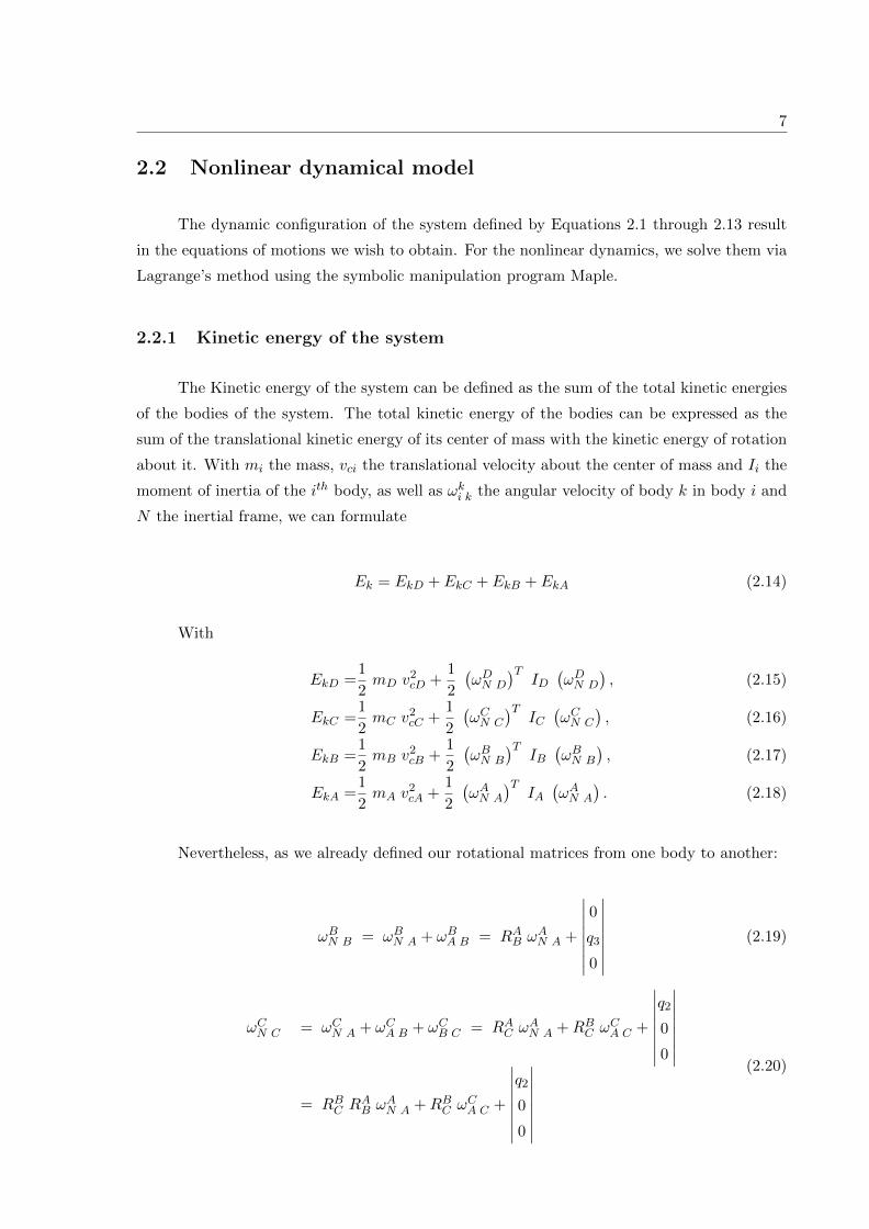
2.2 Nonlinear dynamical model
The dynamic configuration of the system defined by Equations 2.1 through 2.13 result
in the equations of motions we wish to obtain. For the nonlinear dynamics, we solve them via
Lagrange’s method using the symbolic manipulation program Maple.
2.2.1 Kinetic energy of the system
The Kinetic energy of the system can be defined as the sum of the total kinetic energies
of the bodies of the system. The total kinetic energy of the bodies can be expressed as the
sum of the translational kinetic energy of its center of mass with the kinetic energy of rotation
about it. With mi the mass, vci the translational velocity about the center of mass and Ii the
moment of inertia of the ith body, as well as ωki k the angular velocity of body k in body i and
N the inertial frame, we can formulate
Ek = EkD + EkC + EkB + EkA (2.14)
With
EkD =1
2mD v2
cD +1
2
(ωDN D
)TID
(ωDN D
), (2.15)
EkC =1
2mC v
2cC +
1
2
(ωCN C
)TIC(ωCN C
), (2.16)
EkB =1
2mB v2
cB +1
2
(ωBN B
)TIB(ωBN B
), (2.17)
EkA =1
2mA v
2cA +
1
2
(ωAN A
)TIA(ωAN A
). (2.18)
Nevertheless, as we already defined our rotational matrices from one body to another:
ωBN B = ωBN A + ωBA B = RAB ωAN A +
∣∣∣∣∣∣∣∣0
q3
0
∣∣∣∣∣∣∣∣ (2.19)
ωCN C = ωCN A + ωCA B + ωCB C = RAC ωAN A +RBC ωCA C +
∣∣∣∣∣∣∣∣q2
0
0
∣∣∣∣∣∣∣∣= RBC RAB ωAN A +RBC ωCA C +
∣∣∣∣∣∣∣∣q2
0
0
∣∣∣∣∣∣∣∣(2.20)

8
ωDN D = ωDN A + ωDA B + ωDC B + ωDB D
= RAD ωAN A +RBD ωBA B +RCD ωCB C + ωDB D
= RCD RBC RAB ωAN A +RBC RCD ωBA B +RCD ωCB C + ωDB D
(2.21)
Making the assumption that the gimbals are massless, ωDRF D the angular velocity of D
in the reference frame and ID/D the central inertia dyadic of body B, we can formulate the
kinetic energy of the rotor as
Ek =1
2NωD ID/D NωD. (2.22)
As a dyadic is the sum of dyads, vectors placed one to another[7], defining ID/D and
ωDRF D, we can note that
ωDRF D = ω4 a3 + ω3 b+ω2 c1 + ω1 c2; (2.23)
and
ID/D = ID c1 c1 + JD c2 c2 + ID c3 c3 (2.24)
Finally, since the system’s center of mass is fixed in inertial space and as the system is
mechanically conservative, the kinetic energy, EK , of the system under the assumptions is as
well the Lagrangian L, defined as
L = EK = 0.5 ID ω2 (ω2 − sin(q3) ω4) + 0.5 JD ω1 (ω1 + cos(q2) ω3 + sin(q2) cos(q3) ω4) + 0.5 ID
sin(q2) ω3 (sin(q2) ω3 − cos(q2) cos(q3) ω4) + 0.5 JD cos(q2) ω3 (ω1 + cos(q2) ω3 + sin(q2)
cos(q3) ω4) + 0.5 JD sin(q2) cos(q3) ω4 (ω1 + cos(q2) ω3 + sin(q2) cos(q3) ω4) − 0.5 ID
sin(q3) ω4 (ω2 − sin(q3) ω4) − 0.5 ID cos(q2) cos(q3) ω4 (sin(q2) ω3 − cos(q2) cos(q3) ω4)
(2.25)
.

9
2.2.2 Lagrangian of the dynamical system
From Euler-Lagrange equation, with qi and ωi = dqidt the respective position and angular
velocity of body i (i= 1,..,4) along the torques Tk (k = 1, 2) acting on body D and C, we can
define our mechanical system using Equation 2.26.
Note that the nominal mechanism model is found by neglecting torques T3 and T4 acting on
bodies B and A respectively. Nevertheless, they could be defined as additional control inputs
and/or friction.
d
dt
(δ L
δ ωi
)− δ L
δ qi= Tk (2.26)
Finally, substituing the obtained Lagrangian L into the previous equation, we obtain
the equations of motion for our system under the assumptions characterized. The process of
achievement of those equations can be found on the CD attached to the thesis and is done
using the symbolic manipulation program Maple.
2.3 Linear dynamical model
With the resulting nonlinear equations, we can find the linearized ones by the use of
Taylor’s series expansion. We can do this by taking the first terms in the Taylor’s expansion
of the equations describing the model given by the manufacturer obtained by Kane’s method.
Nevertheless, for convenience and readability, the linearized equations describing the whole
system with and without constraints are of the zero order. This was done to be able to
compare the linearized model with the given one. The product of two angles, for the zero
order expansion, was neglected as it tends very fast to zero. The derivation of the linear model
can be found on the CD.
2.3.1 Linearized model about the selected operating points
With the equations obtained for the linear dynamical model, we can acquire the linearized
equations of motion about selected operating points. Those were defined as ω1 = Ω, q3 = q3o
and q2 = q2o, so that
T1 − JD cos(q2o)dω3
dt− JD sin(q2o) cos(q3o)
dω4
dt− JD
dω1
dt= 0 (2.27)

10
T2 + JD Ω cos(q2o) cos(q3) ω4 − JD Ω sin(q2o) ω3 − (IC + ID) dω2dt + sin(q3o) (IC + ID) dω4
dt = 0
(2.28)
−sin(q2o) cos(q3o) cos(q2o) (JC + JD − ID −KC) dω4dt − JD Ω sin(q2o) sin(q3o) ω4 − JD cos(q2o)
dω1dt − (JB + JC + JD − sin(q2o)
2 (JC + JD − ID −KC)) dω3dt + JD Ω sin(q2o) ω2 = 0
(2.29)
JD Ω sin(q2o) sin(q3o) ω3 + sin(q3o) (IC + ID) dω2dt − JD Ω cos(q2o) cos(q3o) ω2 − JD sin(q2o)
cos(q3o)dω1dt − sin(q2o) cos(q2o) cos(q3o) (JC + JD − ID −KC) dω3
dt − (ID +KA +KB +KC
+sin(q2o)2 (JC + JD − ID −KC) + sin(q3o)
2 (IB + IC −KB −KC − sin(q2o)2 (JC + JD − ID
−KC))) dω4dt = 0
(2.30)
2.3.2 Linearized equations for constrained models
All gimbals free of motion
After linearizing our model, we could select our operating points to simplify even further
our model. Recalling ω1 = Ω the spin speed of the rotor disk (body D) and setting q2o = q3o =
0, for all gimbals free of motion we obtain the set of equations defining the dynamical model
as follow
T1 − JDdω3
dt− JD
dω1
dt= 0 (2.31)
T2 − (IC + ID)dω2
dt+ JD Ω ω4 = 0 (2.32)
(JB + JC + JD)dω3
dt+ JD
d2ω1
dt= 0 (2.33)
(ID +KA +KB +KC)dω4
dt+ JD Ωω2 = 0 (2.34)
Under Matlab, the above set of equations were expressed in state space form for purposes
of simulation and control design.

11
All gimbals free of motion except Gimbal #2
While Brake #2 is turned on via the ECP Executive program, bodies B and C become
one. This results in the possible control of their position, q3, by the spin rotor speed or T1.
From Equations 2.31 through 2.34, we could obtain the set of equations defining the system
by setting dω4dt = dω2
dt = 0, resulting in
T1 − JD
(dω1
dt+dω3
dt
)= 0 (2.35)
(JB + JC + JD)dω3
dt+ JD
dω1
dt= 0 (2.36)
This was, once again, rewritten in state space form for convenience under Matlab. More
explicitly
dq3
dt=ω3 (2.37)
dω1
dt=T1
JC + JD + JB(JB + JC) JD
(2.38)
dω3
dt=T1
−1
JC + JB(2.39)
All gimbals free of motion except Gimbal #3
Setting q2o = q3o = 0 and fixing Gimbal #3 so that dω3dt = 0, makes body A and B as
one. Under this configuration, the position and velocity of body A can be controlled by the
rotation of Gimbal #2 with the spin rotor disk. Once again, from Equations 2.31 through
2.34, we could obtain the set of equations defining the system under the set constraints.
T1 − JDdω1
dt= 0 (2.40)
T2 + JD Ω ω4 − (IC + ID)dω2
dt= 0 (2.41)
JD Ω ω2 + (ID +KA +KB +KC)dω4
dt= 0 (2.42)

12
2.4 Computer aided design (CAD) modeling
Autodesk Inventor Professional1 is a 3D mechanical CAD design software for creating 3D
digital prototypes used in the design, visualization and simulation of products. After learning
to work with the software, we succeeded modeling our system and be able to obtain the scalar
moments of inertia Ix, Jx and Kx of each body (x=A,B,C,D) about the ith direction (with
i= 1,2,3) and be able to compare it with the later obtained moments of inertia of each body.
Refer to Figure 2.2 for the software overview.
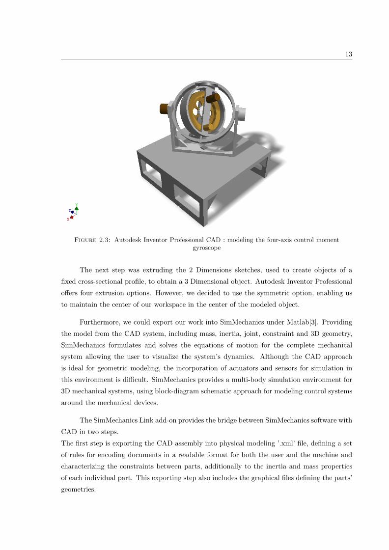
After designing each body and the fasteners that mechanically join between them, we were
able to assemble our system apparent from Figure 2.3
Figure 2.2: Autodesk Inventor Professional CAD : Software overview
From Figure 2.2, we can notice that the scalar moments of inertia of each body can
be obtained separately while accessing their physical properties, after setting up the material
and density of the object. In spite of the difference in shapes and dimensions of every body,
their conception followed a similar itinerary. After selecting the work plane in which we are
sketching, we could draw the geometry in the exact dimensions of our model. These must be
precise, as our final assembly and properties we seek are greatly dependent on it.
1Autodesk Inventor Professional is available to download for students under their website:http://students.autodesk.com/
13
Figure 2.3: Autodesk Inventor Professional CAD : modeling the four-axis control momentgyroscope
The next step was extruding the 2 Dimensions sketches, used to create objects of a
fixed cross-sectional profile, to obtain a 3 Dimensional object. Autodesk Inventor Professional
offers four extrusion options. However, we decided to use the symmetric option, enabling us
to maintain the center of our workspace in the center of the modeled object.
Furthermore, we could export our work into SimMechanics under Matlab[3]. Providing
the model from the CAD system, including mass, inertia, joint, constraint and 3D geometry,
SimMechanics formulates and solves the equations of motion for the complete mechanical
system allowing the user to visualize the system’s dynamics. Although the CAD approach
is ideal for geometric modeling, the incorporation of actuators and sensors for simulation in
this environment is difficult. SimMechanics provides a multi-body simulation environment for
3D mechanical systems, using block-diagram schematic approach for modeling control systems
around the mechanical devices.
The SimMechanics Link add-on provides the bridge between SimMechanics software with
CAD in two steps.
The first step is exporting the CAD assembly into physical modeling ’.xml’ file, defining a set
of rules for encoding documents in a readable format for both the user and the machine and
characterizing the constraints between parts, additionally to the inertia and mass properties
of each individual part. This exporting step also includes the graphical files defining the parts’
geometries.

14
The second step is importing the XML file into Matlab, generating a SimMechanics model,
allowing us to visualize and simulate the system. In the SimMechanic’s model, constraints and
parts of the assembly are defined by joints and bodies.
2.4.1 The mechanical system under SimMechanics
The generated model, including the graphical files defining the geometries of the bodies,
was successfully imported into SimMechanics. Nevertheless, while trying to actuate joints,
their action was not what we expected. SimMechanics defined the rotational axis through the
bolts assembling together the bodies rather than the rotation of the bodies between them-
selves. Although we defined well the constraints between bodies under the CAD platform,
the exportation of the assembly was not usable for a full simulation of the model. The CAD
platform was useful exclusively in terms of visualization of the bodies. The visualization of
our system can be viewed from Figure 2.4.
While inputing some signal on a rotational joint rotating a follower body (F) relative
to a base body (B) about a single rotational axis going through collocated body coordinate
system origins, we were able to collect the angular velocity or acceleration of the follower (F)
via the body sensor blocks. Nevertheless, it is important to consider the units we are working
in to obtain meaningful data. As an example, for body C, we implemented a Sinusoidal input
with amplitude 11 650 counts and frequency 0.4 Hz. The result can be seen from Figure 2.5.
Additionally, the exported block diagram of the system under SimMechanics can be seen from
Figure 2.6 with the individual bodies of our system highlighted.
Figure 2.4: SimMechanics model of our system

15
0 1 2 3 4 5 6 7 8 9 10−4
−3
−2
−1
0
1
2
3
4
Time (sec)
Vel
ocity
(ra
d/s)
Velocity of body C
Figure 2.5: Angular velocity of body C given sinusoidal input
Figure 2.6: Block diagram of the dynamical system under SimMechanics

Chapter 3
Laboratory experiments
To get familiar with a complex system such as the control-moment gyroscope offered
by ECP we had to explore every part of it. From the previous chapter, we derived the
equations of motion of the dynamical model. This chapter deals with the hardware and
software configurations offered by the manufacturer. We will discuss about the experiments
led through the system to obtain its physical parameters and verify the previously obtained
mathematical models.
3.1 Software and hardware setup
3.1.1 ECP Executive software overview
The ECP Executive program is the user’s interface of the system provided by the man-
ufacturer, suitable for Single-Input Multiple-Output (SIMO) and Single-Input Single-Ouput
(SISO) plants control. Its main use is in its communication with the DSP based real-time
controller. Though the non-intuitive application of the system, we succeeded mastering its use
and operation throughout the laboratory experiments we conducted.
The software provides a large range of features. It’s primary use being the specification
and download the low or high order linear control forms of the control algorithms parameters.
Its remaining properties include the input commanded trajectories, input control in continuous
and discrete time forms, collection of data and plotting functions.
17

18
Figure 3.1: ECP background screen display
Top level menu and their description
The top level menu of the ECP Executive software allows us to achieve and implement
several information:
File gives us the possibility to save and open already set parameters so that our work may be
presumed later in time.
Setup provides specification by the user, compilation and implementation of control algo-
rithms, ranging from PID (Proportional-integral-derivative) to high order cascade in contin-
uous time form, via the support of the DSP, or discrete form. It also enables us to set the
sampling rate and specifying direct entry of parameters for the controllers. Finally, it gives
us the option to change working units, such as inches, encoder counts or centimeters (degrees,
encoder counts and radians) for rectilinear (respectively rotational) systems.
Command menu specifies disturbances at the plant output and commanded trajectories in-
puts. The trajectories can take the form of seven sinusoidal or geometric forms, allowing the
characterization of frequency responses of the system. Each trajectory parameters, such as
frequencies, repetition times, dwell times, amplitude, etc., can be specified by the user.

19
Data menu allows the user to select one or more data items to be collected at a chosen multi-
ple of the servo loop closure sampling period after setting commanded trajectories. This data
items range from Control Efforts to Commanded and Encoders Positions. It also allows us to
export data, in our case ideal to have the possibility to work with Matlab.
Finally, the Plot Data menu provides several functions for plotting the data acquired during
the control regulations. It allows up to four acquired data items to be plotted, including ve-
locities and accelerations. Those are generated by numerical differentiation of the data during
the plotting process, which can be a factor to noise amplification as we will see later in this
chapter. Real-time plotting is also available, providing display of acquired data in real-time.
Utility menu, providing configurations of auxiliary DAC’s for outputting analog data in real
time (viewed via spectrum analyzers, oscilloscopes, etc.) was not studied and used in our work.
Background screen display
From Figure 3.1 we can view that the background screen of the software contains the
system status, real-time data and a button allowing us to immediately abort the control effort,
Abort Control. This option enables us to open the control loop and discontinue any action done
by the user, additionally to the red button OFF present on the control box. The Control Loop
Status is describing the status of the control, being Open when the control loop is inactive
and Closed when the user compiles and downloads a control algorithm file into the DSP
board. Moreover, the real-time data permits the user to observe the commanded positions and
encoders positions of the bodies defining the system, additionally to the velocity of the rotor
disk (body D), instantaneously.
The Servo Time Limit defines the status of the implemented algorithm, and will show OK
unless the sampling period does not correspond properly to the compiled algorithm file. While
over-speeding or exceeding the current limits of the motor amplifier, as well as overtaking the
maximum value that Axis #2 position can reach, the Motor Status will display Limit Exceeded.
The Axis 2 V-Brake Off button is the only way to activate the brake about Axis #2.
Exporting data to Matlab
Exporting data from ECP Executive into Matlab is almost immediate. Note that when-
ever we run a new experiment or simply executing a new commanded trajectory, the data of
the previous experiment will be overwritten in the data acquisition memory. We noticed that
saving the plot data from the Plotting menu does not work properly and that whenever we
try to Load the data under the proposed format (*.plt), it often fails to load. Nevertheless,
the Data menu allows us to Export Raw Data under a (*.txt) file format. The saved data is
stored column-wise and can be open with any text editor or system terminal.
20
To modify the text file into a readable format for Matlab, as an .m file, we edit our file as
follow:
• We comment the first row, containing the information about each column such as Time,
Commanded position, etc., with ’%’.
• Before the opening bracket ’[’, we enter a name for our column-wise data, such as data=.
• We put a semicolon ’;’ after the closing bracket ’]’.
• In the last lines of our file, we will define the time t, input u and output y vectors by
selecting the appropriate and chosen columns. With ni (i = 1..10) the selected column
corresponding to the appropriate data we would like to study, the last three lines of our
text file will look as follow:
t=data(:,ni);
u=data(:,ni);
y=data(:,ni);
• Finally, we save the file with the extension .m, resulting in a script Matlab can run and
read the measurements for our three defined vectors. The user should confirm that the
units from the ECP Executive software are corresponding to the desired ones.
3.1.2 Hardware installation and operation
After granting Administrator’s rights under Windows operating system, we installed the
ECP Executive software. We connected the 60-pin flat cable male Header, located at the
edge of the DSP board, and inserted it into an empty slot of the PC’s Peripheral Component
Interconnect (PCI) bus. After locating the new hardware manually, Windows recognizes the
PCI DSP Board. The next step is accessing, detecting and communicating the ECP software
with the board. This is done automatically after first launch of the ECP Executive software.
The other end of the 60-pin flat cable should now be connected to the Amplifier Box itself.
Finally, after connecting the power supply cord of the Amplifier Box, we connected it via
the two supplied cables with the model mechanism.
As our Windows is a non-American English version, we had to change the decimal point from
’,’ to ’.’ in the Control Panel.
One of the most important features for the system to work properly is the Power ON
and OFF procedure. To turn ON the power, we first turn ON the PC and after launching the
ECP executive program we turn ON the Amplifier Box. Vice versa, to turn the power OFF,
we first turn OFF the Amplifier Box and then close the ECP executive program.

21
It is also good to reset the DSP board before each maneuver of the system. This can be
done under the Utility menu, via Reset Controller.
Real time Control implementation - Drive Amplifier
The control system of the model is defined by three distinct subsystems: the ECP
Executive user interface software, the mechanism and the real-time controller.
After implementing the control algorithm specified by the user, it is downloaded from the ECP
Executive interface to the DSP board, executed in the specified sampling rate. This results in
outputting the digital control effort signal to the DAC. The analog voltage, outputted from
the DAC, is converted into current via the servo amplifier and then torque via the motors. The
plant’s dynamics outputs are sensed by encoders, establishing a stream of pulses decoded by
a counter on the DSP board, which are digitalized for the real-time control algorithm. Mind
that any data specified by the user is stored in the memory of the DSP board and uploaded
to the PC memory for plotting after the end of each manipulation. An overview of the control
system can be observed from Figure 3.2.
Figure 3.2: Overview of the real-time control system
Our brushed DC motors are internally commutated electric motors run from direct
current power sources[6]. At the kth sampling period, the input to the 16-bit DAC is the
control effort, providing analog signal for the motor amplifier. The amplifier is working as an
Operational Transconductance Amplifier (OTA) whose differential input voltage produces an
output current for the motor[1]. To introduce the demanded current by the motor, an analog
proportional integral (PI) controller is applied to the amplifier.

22
The gains of the analog PI controller are such that the dynamics of the current are faster
than the dynamics of the mechanical plant. This results in a steady state value of the current
achieved immediately with respect to changes in positions, and thus velocities. The mechanism
drive block diagram can be seen from Figure 3.3
Figure 3.3: Mechanism drive block diagram
Providing analog signal to the servo amplifier from the control effort passing through
the DAC, with kDAC the DAC gain in volts per counts, the signal passes through the amplifier
gain kA resulting in a voltage proportional to the desired current. The proportional gain, kP ,
and integral gain, kI , of the amplifier are chosen to be very high with respect to the inner
back emf loop within the range of the motor operation. The motor admittance, defined by its
inductance and resistance, results in its flowing current. This current is then subtracted, as a
voltage proportional to the motor current, from the voltage proportional to the desired current.
The given torque is then delivered to the sliding rod after passing through the DAC again.
While taking into account the plant dynamics, H(s), the torque results in the shafts angular
velocity, defined by ω, subtracted from the voltage passing through the Servo Amplifier.

23
3.2 Experiments for determining the physical parameters of
the system
In this section we will deal with experiments on the real model to identify the plant’s
parameters and characteristics. This will be in the form of implementation of control schemes.
We will first identify several moments of inertias, the less amenable to mass property calcula-
tions, then calculate the control effort gains and the feedback sensor gains and finally determine
the friction acting on the rotor disk.
3.2.1 Measurement of inertias
We will measure three selected moments of inertia, IC , KA and JC , using the principle
of conservation of angular momentum. The configurations for the moment of inertias tests can
be inspected from Figure 3.4. The calculation of all moments of inertia can be found in the
CD attached to the thesis.
Figure 3.4: Configuration of the system for the selected moments of inertias experiments
Inertia test - JC
For the moment of inertia JC , we set the mechanism as shown in Figure 3.4. Body A was
rotated until we found a location with the least friction acting on it, leading to initialization
of the encoders values at the gimbal positions to zero. Furthermore, after setting the sampling
period, we wrote a simple real-time algorithm to activate Motor #1. In addition, we set an
input impulse trajectory of 16 000 count, with a pulse width of 1000 ms and two repetitions,
meaning a positive-going step of 16 000 count followed by a negative-going step of the same
number of counts. After making sure we set up the data acquisition required, we executed the
trajectory and plotted the Encoder 1 Velocity and Encoder 3 Velocity.
24
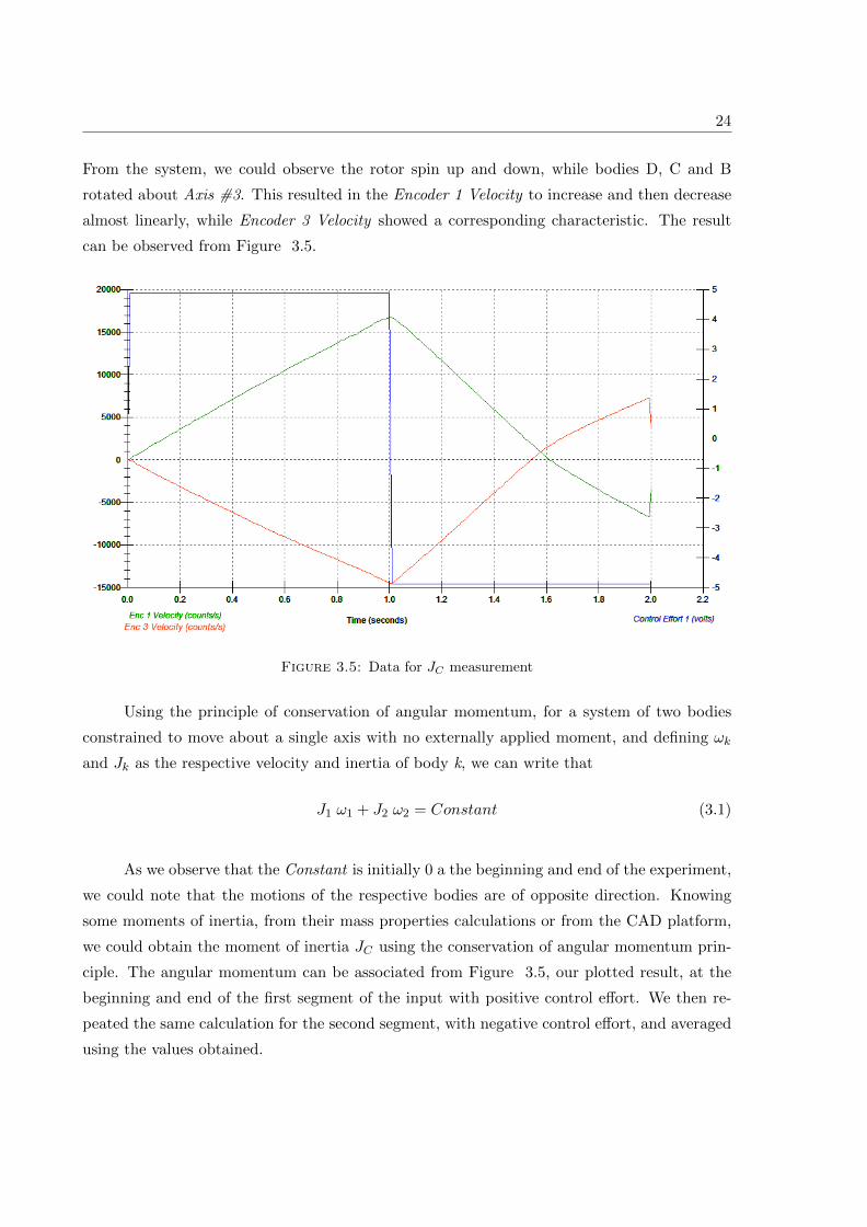
From the system, we could observe the rotor spin up and down, while bodies D, C and B
rotated about Axis #3. This resulted in the Encoder 1 Velocity to increase and then decrease
almost linearly, while Encoder 3 Velocity showed a corresponding characteristic. The result
can be observed from Figure 3.5.
Figure 3.5: Data for JC measurement
Using the principle of conservation of angular momentum, for a system of two bodies
constrained to move about a single axis with no externally applied moment, and defining ωk
and Jk as the respective velocity and inertia of body k, we can write that
J1 ω1 + J2 ω2 = Constant (3.1)
As we observe that the Constant is initially 0 a the beginning and end of the experiment,
we could note that the motions of the respective bodies are of opposite direction. Knowing
some moments of inertia, from their mass properties calculations or from the CAD platform,
we could obtain the moment of inertia JC using the conservation of angular momentum prin-
ciple. The angular momentum can be associated from Figure 3.5, our plotted result, at the
beginning and end of the first segment of the input with positive control effort. We then re-
peated the same calculation for the second segment, with negative control effort, and averaged
using the values obtained.

25
We can solve for the unknown inertia, with ωib and ωif the respective first and final
angular velocities of body i, the following
J1 ω1b + J2 ω2b = J1 ω1f + J2 ω2f (3.2)
Resulting in:
J1 = −J2(ω2f − ω2f )
(ω1b − ω1b)(3.3)
Finally, taking into account the brakes and configuration of the system during the ex-
periment, we can determine:
J1 = JC + JB and J2 = JD (3.4)
JD and JB are assumed to be known, from previous measurements or direct calculations,
enabling us to determine the moment of inertia JC .
Inertia test - KA
For the second inertia test, KA, we set the mechanism as defined in Figure 3.4. With
the real-time algorithm staying the same, activating Motor #1, we changed the pulse width
of the input impulse trajectory to be 2 000 ms while leaving the rest of the parameters as for
the inertia test of the moment of inertia JC .
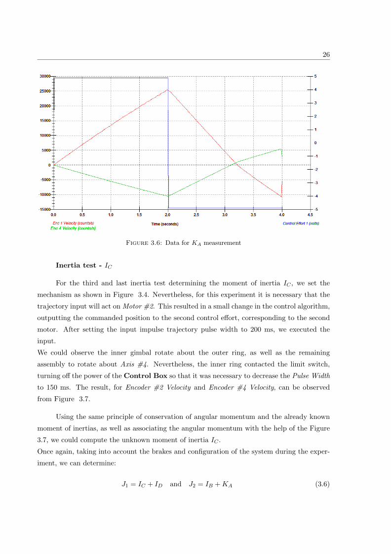
After executing the trajectory, we could observe the whole system rotate about Axis #4. The
result for Encoder #1 Velocity and Encoder #4 Velocity can be observed from Figure 3.6.
Using again the principle of conservation of angular momentum and the already known
moment of inertias, as well as associating the angular momentum with the help of Figure 3.6
resulting from positive and negative control effort respectively, we can compute our unknown
moment of inertia.
Taking into account the brakes and configuration of the system in this experiment, we can
determine:
J1 = KA +KB + JC and J2 = JD (3.5)
As we assume we know JD, KA and KB from previous measurements, adding at this
time JC from the previous experiment, we determined KA.
26
Figure 3.6: Data for KA measurement
Inertia test - IC
For the third and last inertia test determining the moment of inertia IC , we set the
mechanism as shown in Figure 3.4. Nevertheless, for this experiment it is necessary that the
trajectory input will act on Motor #2. This resulted in a small change in the control algorithm,
outputting the commanded position to the second control effort, corresponding to the second
motor. After setting the input impulse trajectory pulse width to 200 ms, we executed the
input.
We could observe the inner gimbal rotate about the outer ring, as well as the remaining
assembly to rotate about Axis #4. Nevertheless, the inner ring contacted the limit switch,
turning off the power of the Control Box so that it was necessary to decrease the Pulse Width
to 150 ms. The result, for Encoder #2 Velocity and Encoder #4 Velocity, can be observed
from Figure 3.7.
Using the same principle of conservation of angular momentum and the already known
moment of inertias, as well as associating the angular momentum with the help of the Figure
3.7, we could compute the unknown moment of inertia IC .
Once again, taking into account the brakes and configuration of the system during the exper-
iment, we can determine:
J1 = IC + ID and J2 = IB +KA (3.6)

27
Figure 3.7: Data for IC measurement
As we assume we know ID, IB and KA from previous measurements, we determined the
moment of inertia IC .
3.2.2 Measurement of the control effort gains
For control design purposes, it is necessary to implement the control effort gain of the
model. Those gains kui (i=1,2) can be defined at time zero, with no initial rotation, as the
ratio between the respective torque Ti and control effort ui associated with the ith plant input.
Additionally, it can be defined as the product of the DAC gain, kDAC , with the Servo Amp
gain, ka, with the motor torque constant, kt, and the drive pulley ratio kp. The configuration
of the system for both our control effort gains, ku1 and ku2, can be observed from Figure 3.8.
For calculations of those gains, please refer to the attached CD.
Ti = ui kui (3.7)
and
kui = kt kp kt kDAC (3.8)

28
Figure 3.8: Configuration of the system for the control effort gain tests
Control effort gain - ku1
The control effort gain for this test is measured using Newton’s second law for a rota-
tional body, with the torque equal to the product of the body’s moment of inertia and of its
acceleration, as in Equation 3.9.
T = Jd ω
dt= J
d2 q
dt2(3.9)
We inputted some known positive and negative control effort signal to the rotor disk,
body D, and observed its accelerations. As we know the rotor inertia value and are able to
observe the accelerations, we will be able to determine the applied torque, hence the control
effort gain.
Before implementing the control algorithm, the same we used for the inertia tests of KA and
JC , activating Motor #1, we configured our system as shown from Figure 3.8 for the control
effort gain experiment of ku1. The input impulse trajectory was specified with an amplitude
of 16 000 count, a pulse width of 4 000 ms and two repetitions.
After executing the input, we could observe the rotor spin up and down. We can perceive the
obtained result on Encoder #1 Velocity and Control Effort #1 from Figure 3.9.
The fact that the acceleration is of lesser magnitude that the deceleration is due to the
friction from the rotor, as it acts at the opposite direction of the motion of the disk. From the
obtained values, the control effort gain is a result of direct application of Equation 3.9.

29
Figure 3.9: Data for ku1 measurement
Control effort gain - ku2
The control effort gain for this test is measured using the gyroscopic cross product, with
the torque equal to the product of the body’s momentum, M, with the angular velocity, ω,
associated with change of direction of the vector M. The momentum will change direction for
the necessary applied torque T.
T = M ω (3.10)
The experiment consist of measuring the required torque necessary to change the direc-
tion of the angular momentum at a rate ω.
We first initialized the rotor speed to 400 RPM. We could note that while applying a light
pressure on the inner ring edge, it effects the torque about Axis #2, causing the momentum
vector to precess at velocity ω in the q4 direction. Nevertheless, if the pressure applied is
constant, the precession rate will be constant. This is due to the gyroscopic precession, or
torque-induced precession. It is a phenomena in which the axis of the spinning object quake
when a torque is applied to it, causing the distribution of force around the acted axis[2]. In
addition, we applied pressure to the edge of body A, rotating the assembly about Axis #4.
The torque is then negative about this axis, causing the momentum to precess at velocity ω
in the q2 direction. Furthermore, we set the control algorithm to regulate the position of Axis
#2 and keep it at its current position. For measuring the control effort required to fulfill this
requirement, we set an input impulse trajectory with amplitude 0 counts to be able to collect
data after executing it. We then slowly rotated the assembly about Axis #4, causing between

30
4 to 6 Volts of control effort, observable on the background screen of the ECP executive pro-
gram as in Figure 3.1. We let the assembly spin freely and reversed the direction to achieve
between -6 to -4 Volts of control effort, releasing the assembly again so it spins freely. We can
perceive the obtained result on Encoder 4 Velocity and Control Effort 2 acquired data from
Figure 3.10.
Figure 3.10: Data for ku2 measurement
Finally, we could obtain the control effort gain from direct application of Equation 3.10.
3.2.3 Measurement of the encoder gains
Our system is partially composed of optical encoders with counts as output. We mea-
sured the change in sensor signal output per unit of physical position change, in other words
the sensor gains.
To identify those gains, we turned off all brakes and selected zero position to zero the
incremental encoders values at their current position. We then marked the initial position of
Body A and B, and rotated them about Axis #4 and Axis #3, respectively, until a complete
revolution is achieved. We then noted the obtained number of counts for the respective bodies,
available from the background screen of the ECP Executive program. For Body C, as the
motion is restricted by the limit stops, we rotated only for half a revolution and noted the
obtained number of counts. The gain for Encoder #1 was given by the manufacturer, as it is
physically inaccessible to reach the spin rotor.

31
The controller firmware multiplies the encoder and commanded position signals by 32,
so that we have to multiply the measured encoder gains by this value for them to be properly
scaled for the system. As we noted the obtained counts we have got per revolution, and
knowing that one revolution is approximately equal to 6.283 radians, Table 3.1 sums up the
obtained encoder gains.
Encoder - Axis Output/Revolution (counts/rev) Gain (counts/rad)
4 16 000 2547.5·32
3 16 000 2547.5·32
2 24 400 3883.4·32
1 6 666 1061·32
Table 3.1: Encoder gains
Furthermore, the obtained measured moments of inertias from the experiments, in bold,
and mass property calculations are summarized in Table 3.2. The control effort gains were
summarized in Table 3.3.
Body Inertia Element Value (kg.m2)
A KA 0.0682
IB 0.0131B JB 0.0189
KB 0.032
IC 0.009C JC 0.0272
KC 0.0162
ID 0.0166D JD 0.0333
KD 0.0166
Table 3.2: Moments of inertia
Control effort gain Value (N/count)
ku1 1.9879 · 10−5
ku2 8.9862 · 10−5
Table 3.3: Control effort gains
Note that the remaining moments of inertias were obtained via the mass property cal-
culations, such as mechanical geometries, material densities, and weights of the components
defining the system. Those can be found on the CD attached to the thesis.
3.2.4 Measurement of the friction acting on the rotor disk
The friction acting on body D is not negligible. To determine it, we tried to achieve
a steady velocity for a given control effort. Nevertheless, the ECP Executive software does
32
not allow us to reach it, as the width for any input trajectory can not exceed 32 seconds. As
we know, the transfer function of the motor’s mechanical part is defined as ktJs+b , with kt the
torque gain of the motor, J the moment of inertia about the body it acts on and b the friction
acting on the body. In addition, we know the moment of inertia of body D around its axis of
rotation, as well as the given torque gains, so that we can determine the friction acting on it.
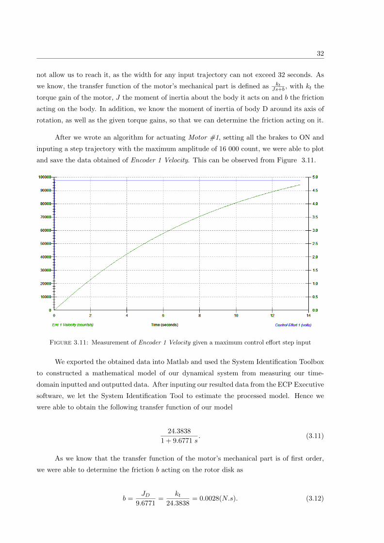
After we wrote an algorithm for actuating Motor #1, setting all the brakes to ON and
inputing a step trajectory with the maximum amplitude of 16 000 count, we were able to plot
and save the data obtained of Encoder 1 Velocity. This can be observed from Figure 3.11.
Figure 3.11: Measurement of Encoder 1 Velocity given a maximum control effort step input
We exported the obtained data into Matlab and used the System Identification Toolbox
to constructed a mathematical model of our dynamical system from measuring our time-
domain inputted and outputted data. After inputing our resulted data from the ECP Executive
software, we let the System Identification Tool to estimate the processed model. Hence we
were able to obtain the following transfer function of our model
24.3838
1 + 9.6771 s. (3.11)
As we know that the transfer function of the motor’s mechanical part is of first order,
we were able to determine the friction b acting on the rotor disk as
b =JD
9.6771=
kt24.3838
= 0.0028(N.s). (3.12)

33
3.3 Verification of the mathematical model
After we determined the linearized equations describing the dynamics of our model, we
were able to compare them, given initial conditions, with real data using the ECP Executive
program maneuver and plotting tool. We observed the encoders positions and velocities for
different initial conditions, setting different constraints for our system corresponding to the
developed constrained mathematical models.
3.3.1 For all gimbals free of motion
From equations 2.31 through 2.34, our linearized model is available for the free rotation
of all gimbals. After setting our system with the same configuration as for the moment of inertia
JC experiment and additionally turning off all brakes, we actuated Motor #1 with an input
step trajectory with amplitude 4 800 count for 15 000 ms. We were able to plot the result,
using the plotting option from the ECP Executive software, and observe Encoder 1 Velocity,
Encoder 3 Position and textitEncoder 3 Velocity for the given input examined from Figure
3.13.
Comparing the obtained result with the mathematical model from the linearized equations and
building a Simulink block diagram from the resulting state space realization with a comparable
input, we obtained what can be seen from Figure 3.12. The state space realization is present
on the CD attached to the thesis.
We can note that the mathematical model is corresponding to the real one given same input.
Nevertheless, we can discern nutation in Encoder 3 Velocity from the real model, function of
the wheel speed. This nutation can be damped throughout rate feedback at Gimbal #2, and
will be studied in the next chapter.
34
Figure 3.12: Mathematical model for all free gimbals : Encoder 1 Velocity and Encoder 3Velocity and Position given a step input
Figure 3.13: Real model for all free gimbals : Encoder 1 Velocity and Encoder 3 Velocityand Position given a step input

35
3.3.2 For all gimbals free of motion except Gimbal #2
After setting our system with the same parameters as for the second moment of inertia
experiment, Jc, which we can observe from Figure 3.4, we actuated Motor #1 with an input
step trajectory with amplitude 4 800 count for 15 000 ms. As the brake of Axis #2 was on,
we wanted to examine the effect the rotor disk as on Encoder 3 Position and Velocity. As
expected,Encoder 3 Position went in the opposite direction of the rotor disk displacement and
we were able to plot the result using the plotting option from the software.
To be able to compare it with our mathematical model, we used our constrained linearized
model, from Equations 2.35 and 2.36, and built a state space realization of the plant linearized
about any gimbals angles q2o, q3o and angular velocity of the rotor disk ω1. In addition, we
made sure to constraint the model as we did for the real model simulation. Finally, we built
a Simulink block diagram, taking into account the A, B and C matrices describing the system
and set a step input of same amplitude as done for the real model experiment, making sure
we use the same units. The state space realization can be viewed from the ’.m’ file present on
the CD.
We can clearly discern that the constrained mathematical model obtained in Chapter 1 is
comparable to the real model.
Figure 3.14: Comparison of real model and mathematical model of Encoder 3 Position givena step input

36
3.3.3 For all gimbals free of motion except Gimbal #3
From equations 2.40 through 2.42, our linearized model is available for the system
with Gimbal #3 locked. After setting our system with the same configuration as previously,
turning on just Axis 3 Brake, we actuated motor #2 with a sinusoidal input trajectory with
the selected amplitude to be equal to 1 500 count and frequency 5 Hz. We also initialized
the rotor speed to 50 RPM. The input was selected to be sinusoidal, as Body C can not
exceed more than a revolution with respect to Axis #2. Furthermore, we were able to plot
the result, using the plotting option from the software, and observe Encoder 2 Velocity. It
was interesting to observe the action of Motor #2 on Encoder 4 Velocity for the given input.
Nevertheless, we can observe from Figure 3.16 certain picks of velocities that are not present
in the mathematical model. This is due to the ECP Executive software and the small noise
that could be identified from Encoder 4 Position, as the velocity is directly obtained from the
derivative of the position.
After obtaining the mathematical model from the linearized equations and building a block
diagram from the resulting state space realization with similar inputted trajectory, we could
confirm our model.
Figure 3.15: Mathematical model for Gimbal #3 Locked : Encoder 2 Velocity and Encoder4 Velocity given sinusoidal input
37
Figure 3.16: Real model for Gimbal #3 Locked : Encoder 2 Velocity and Encoder 4 Velocitygiven sinusoidal input


Chapter 4
Feedback control
In this chapter we will deal with control algorithms under the ECP Executive program.
This will be done after going through the structure of the control algorithms possible to
implement. Finally, we will implement position control using Cascade method for body C and
D.
4.1 Setting a feedback control in the ECP environment
In the Setup top level menu we can find the Setup Control Algorithm option. This
option allows the user to write a control algorithm for compilation and implementation via the
DSP board controller.
The Sampling Period allows the user to change the servo period in multiple of 0.000884,
starting from 1.1 KHz sampling frequency. Nevertheless, while the written control algorithm
is complex or long, the user should increase the sampling time or reduce execution time of the
servo algorithm. In the case the execution time is longer that the sampling period, the Real-
time Controller will be opened automatically while the Servo Time Limit on the background
of the ECP Executive software will display its status as Exceeded.
The user can also observe a User Code view box with the latest loaded or written algorithm.
The Edit Algorithm option will enable the user to open the servo algorithm in the ECP Editor,
as well as saving the changes made. In case the user is not able to access the ECP Executive
software, it is possible to write the servo algorithm in any text editor and save it with the
extension ’.alg’. After writing or loading from the disk, as well as editing the algorithm, the
user will need to download it from the editor to the Real-time Controller by choosing Implement
Algorithm.
Note that the Editor is not case sensitive.
39

40
4.1.1 Structuring the Control Algorithm
The structure of the control algorithm is made of three sections. Definition of variables,
initialization of variables and finally the real-time or servo loop execution. After implement-
ing the algorithm, the internal variables, defined from q1 to q100, are assigned to the defined
variables. Coefficients running the servo loop code, remaining constant or initialized to certain
values, and the assigned values of the servo gains are then initialized. Finally, the condition
statements as well as the assignments that are stated in the servo loop code segment, starting
with ”begin” and ending with ”end”, are executed every Sample Period.
Defining variables
The user is given a possibility to define 100 general variables for gains, controller coeffi-
cients and variables used by the Real-time Controller and stored as floating point numbers. In
addition to these general variables, 8 global variables are available, containing instantaneous
commanded positions, encoder positions, as well as control effort. To assign a name N to the
general variable qi (i = 1, .., 100), the user could use the #define statement as such:
#define N qi
The ECP Executive program offers the user to inspect critical internal variables of their
control algorithms by using the special general variables q10 to q13 found in the Data Acquisi-
tion library as collectible data. The 8 global variables are
control effortK with K = 1, 2
encE pos with E = 1, .., 4
cmdC pos with C = 1, 2
Initializing variables
The controller coefficients running the servo loop code, the assigned values of the servo
gains and the values of the algorithm’s variables, are initialized after defining the variables.
Those values should be assigned before or after the servo loop code segment to be able to
maximize its execution speed. To assign a value V to the given name N of the selected general
variable qi, the user could write as such:
N = V

41
Initializing the rotor speed
In case that the user initialized the rotor speed and wishes to implement a control
algorithm to regulate it, thus having the control effort1 as an output, he should include the
statement m136 = 0 in the initialization segment of its algorithm. This as to effect to suppress
the control done automatically by the board controller to remain the rotor speed to a constant
value.
Servo loop code segment
The condition statements and legitimate assignments that are stated in the servo loop
code segment will be executed every Sample Period. The Servo loop code starts with a ”begin”
and ends with an ”end”, and can contain the four standard arithmetic operators *, /, + and
-, which are applied following the precedences rules. In addition to that, the modulo operator
% lets the user the possibility to produce the resulting remainder in the case the value in front
of this operator is divided by a value after it.
Consider that the functions on a certain expression can be defined as:
function (expression)
Tables 4.1 and 4.2 list, respectively, the functions and comparators determining the truth
of a condition via the if statement offered by the editor.
Function Description
sin standard trigonometric sine function
cos standard trigonometric cosine function
tan standard trigonometric tangent function
asin arc sine function (inverse sine) with range −π2 to
π2
acos arc cosine function (inverse cosine) with range 0 to π
atan arc tangent function (inverse tangent) with range −π2 to
π2
sqrt square root function
abs absolute value function
exp exponential function
ln logarithmic function (log base e)
int truncation function returning the greatest integer equal or less to the argument
Table 4.1: Functions available through the ECP Executive editor

42
Comparator Description
> greater than
< less than
! > not greater than or equal to
! < not less than or equal to
= equal to
! = not equal to
Table 4.2: Comparators available through the ECP Executive editor
The conditional execution of segments of the code are done through the if statement.
If the condition is true, then the Real-time Controller will execute all sequences following
it. The condition is done by the comparators defined in Table 4.2 and can be composed of
several comparators by the use of and and or operators. The conditional segments are of the
form:
if (condition1 and condition2)expression.elseexpression.endif
From the following code we can find an example of a written control algorithm program.
This controller represents a simple control loop about Axis #2 with the rest of the axes
stationary.
; Definition of variables
#define pos2_past q18 ; past encoder 2 position
#define enc2_dif q19
#define kp q20 ; proportional gain
#define kd q21 ; derivative gain
#define Ts q22 ; sampling time
#define kdd q23 ; discrete - saving real -time processing
;Initialization of variables
Ts =.00884 ; Initializing the sampling time
; Note: set it in the Setup Control Algorithm as well , here defined locally
kp=1.8 ; initializing proportional gain
kd=0.2 ; initializing derivative gain
kdd=kd/Ts ; Discrete controller
;Servo loop segment
begin
control_effort2 =(kp*(cmd1_pos -enc2_pos)-kdd*(enc2_pos -pos2_past )) ; control law
past_pos2=enc2_pos
end

43
4.1.2 Control Algorithm under the ECP Executive program
In this subsection, we will go through real-time control algorithms and implement them.
We will then acquire the data and plot it. All control algorithm are available through the CD
attached to the thesis.
Proportional derivative (PD) control loop about Axis #2
From the Laplace transform of Equations 2.32 through 2.34, the transfer function
between Encoder 2 Position and Torque #2 can be described as in 4.1. We wrote the control
algorithm as a simple PD control loop about Axis #2, with the remaining axes stationary.
The apparatus is configured as in the measurement of moment of inertia JC , from Figure 3.4,
with brake 3 and 4 on.
After implementing the algorithm, we could observe that the gimbal about Axis #2 resists
to disturbances. We then set data acquisition for Commanded 1 Position, Encoder 2 Position
and Control Effort 2, and executed a step input trajectory with amplitude 1000 count, dwell
time of 5000 ms and one repetition. The result can be observed from Figure 4.1.
Note that the proportional and derivative gains, respectively kP and kD, were selected using
root locus, a method plotting the poles of the closed loop transfer function as a function of
the gain parameters. Knowing the transfer function describing our system and using rltool,
a root locus design using MATLAB’s Graphical User Interface, we were able to obtain kP and
kD by entering design parameters such as natural frequencies and settling time by inputing
design constraints. This resulted in the design window to display a region reflecting the set of
the determined design specifications, so that we obtained kP = 4 and kD = 0.3.
q2(s)
T2(s)=
ID +KC +KB +KA
J2D Ω2 + (ID +KC +KB +KA)(ID + IC) s2
(4.1)
PD and PID control of the inner assembly about Axis #3
From the transfer functions coming from equations 2.35 and 2.36 of the linearized
model when Gimbal #2 is locked, Motor #1 is acting upon bodies C and B affecting their
displacement q3. This is due to the torque reaction, consequence of the law of conservation of
angular momentum. The selected PD controller includes the hardware gains.
44
Figure 4.1: PD control about Axis #2
Considering we have a second order transfer function, from reference input to position
q3 of the canonical form
H(s) =ω2n
s2 + 2 ζ ωn s+ ω2n
, (4.2)
We can define the natural frequency ωn and damping coefficient ζ considering kp and kd
the respective proportional and derivative gains of our PD controller, as
ωn =√
(ku1ke3
kp
JB + JC) (4.3)
and
ζ =ku1ke3
kd
2 (JB + JC) ωn(4.4)
Supposing that the apparatus is configured as in the measurement of moment of inertia
JC , from Figure 3.4, we wrote a real-time algorithm implementing a PD controller about Axis
#3.

45
Knowing the proportional gain kP with respect to ωn, selecting kP = 2.5 and kP = 5,
the system should behave like a 1.652 Hz and a 2.335 Hz spring-inertia oscillator, respectively.
After setting up a closed loop step input of 0 count amplitude to be able to collect data, we
implemented the algorithm with both values of kP . Finally, after executing the null input,
we applied a small disturbances about Axis #3. The obtained oscillations of the assembly
due to this disturbances can be observed from Figure 4.2. The system behaves like a 1.652
Hz oscillator, observed from the right, and a 2.335 Hz oscillator, observed from the left as
expected.
Figure 4.2: Oscillating system responses for different values of kP
Following the equations for the natural frequency and damping coefficient, we set the
derivative gain kD for two different damping cases - under-damped and critically damped. The
set up trajectory was a step input with amplitude 300 count for a dwell time of 5000 ms and
one repetition. We collected data for the Commanded 1 Position and Encoder 3 Position.
This can be observed from Figure 4.3.
For the PID controller, we computed the integral gain ki such that ki ke3 ku1 = 30
N-m/(rad-sec), and implemented a controller with kD and kP as in the critically damped case
from Figure 4.3(b). We used the integral part of the controller to eliminate the steady-state
error to the step input. The result can be observed from Figure 4.4. We can observe from the
real model the integral action decreasing the steady-state error.

46
(a) Underdamped case with kD = 0.22
(b) Critically damped case with kD = 1.4
Figure 4.3: PD control about Axis #3 with kP = 8.2 and different values of kD
Control of Axis #4 position by torquing Axis #2 motor
The control of Axis #4 position is done by torquing the Axis #2 motor. The actuation
of Axis #4 is done by gyroscopic torque, which we can use to control its position. Taking
into account the hardware gains, and knowing from Equations 2.40 through 2.42 the transfer
functions of q2(s)T2(s) and q4(s)
T2(s) , we can use the successive loop closure (SLC) method to create
our control[5]. This method requires the system to be initially decoupled into more than one
single-rate subsystems, which involves any methodologies for designing the control of each
loop. The successive loop closure diagram can be seen from Figure 4.5.

47
Figure 4.4: Control using the proportional and derivative gains as in the critically dampedcase with integral gain ki = 17
In our case, we will first close a rate feedback loop around the angular velocity ω2 of body C,
damping the nutation mode. We will then deal with the outer loop to be able and control the
position q4 about Axis #4.
With the configuration of the apparatus as in the measurement of moment of inertia JC , from
Figure 3.4, with only Axis #3 Brake on, we know that the nutation of the gyroscope is highly
dependent of the wheel speed[2]. The damping of this nutation can be led through the rate
feedback at Gimbal #2. Assuming the damping control effort to be u2damping = −kv q2 s, the
higher rate feedback gain kv, the higher damping is observed on Encoder 2 Velocity. Leading
experiments with different values for the rate feedback gain, we noted that a value of kv = 0.9
resulted in an almost critical damping with the rotor speed of about 300 RPM.
Figure 4.5: Successive loop closure control diagram

48
After initializing our rotor speed to 300 RPM, and implementing the written control
algorithm inspired by Figure 4.5, we noticed that any disturbance caused about Axis #4 is
regulated by the inner assembly about Axis #2. The proportional and derivative gains of the
PD controller were chosen with the generation of the root locus of the outer ring, using rltool
under Matlab. In addition, we input a step trajectory of 400 count and 200 count amplitude
with 2000 ms dwell time, and observed the Commanded Position 1, the Encoder 4 Position as
well as the Control Effort 2. After adjusting the gains to achieve the overshoot to be less than
10% and rise time less than 500 ms, we obtain the results from Figures 4.6 . We can observe
that the 400 count step input trajectory results in a clear DAC saturation that is, as we know,
10 volts. Nevertheless, we can see that it is not the case while inputting a step trajectory of
200 count.
From Figures 4.7(a) and 4.7(b), we can observe the Control Effort 2 and Encoder 2
Velocity for a ramp input trajectory with distance of 6000 count, dwell time of 1000 ms and
velocity of 3000 counts/sec. We can see the close tracking at each end of constant velocity
section. Those rapid accelerations, impulsive type shapes, are possible due to the gyroscopic
control actuation, as well as the associated rotor’s transfer of momentum, as it is not possible
for the small actuator, Motor #2, to act as such on the whole assembly.
4.2 Controlling the positions of body C and D using Cascade
control
Possessing the dynamics of our system, we consider the analog PI controller gains of the
amplifier such that the dynamics of the current loop are much faster relative to the dynamics
of the mechanical part of the plant. This results in a steady state value of the current to
be achieved almost instantaneously relative to changes in velocities and positions. Using
cascade control, we can decompose our control of angular velocities and position into loops.
Considering the transfer function of the inner current control loop to be equal to one, so that
its output closely tracks its reference input, allows us to greatly simplify the control of the
angular velocity of the respective body considering it as an outer loop. Furthermore, by adding
another loop exterior to the angular velocity control loop, we could control the positions of
the respective bodies[4]. From Figure 4.9, we can note that we saturated the input current.
It is also important to note that a large change in set point could occur and that the integral
terms of our PID controller could accumulate a significant error during the rise period. This
could lead in excess overshooting as the error accumulates. From Figure 4.8, we could see the
effect of a simple anti-windup back-calculation method on the PID controller with respect to
the set current saturation of Motor #1.

49
(a) 200 count step input - no saturation
(b) 400 count step input - DAC saturation
Figure 4.6: Gyroscopic torque control using successive loop closure and PD for differentinput step trajectory
We considered the parameters of both motors to be as in Table 4.3.
Motor Continuous current (amps) Torque constant (mN-m/amp)
1 2.15 52.5
2 0.9440 81.91
Table 4.3: Motors specifications

50
(a) Results with control effort
(b) Results with Encoder 2 Velocity
Figure 4.7: Gyroscopic torque control using successive loop closure and PD for input ramptrajectory
After setting a PID controller, with selected gains using root locus for the inner loop
controlling the angular velocities of body D and C, we were able to control their position using
a PD controller. For both angular velocties, we selected kP to be equal to 6, kI to 6 and
kD to 0.6. To control the position we selected a PD controller. For controlling the position
of body C, we used the PD gains we obtained in the previous PD control about Axis #2
from root locus, respectively kP=4 and kD=0.3. For body D, we selected the PD gains to be,
respectively, kP=5 and kD=0.4. The resulting controls of the respective bodies D and C can
be seen from Figure 4.10 and Figure 4.11. The chosen design requirements, with the percent
overshoot < 15% and settling time < 1.5 seconds, were respected.
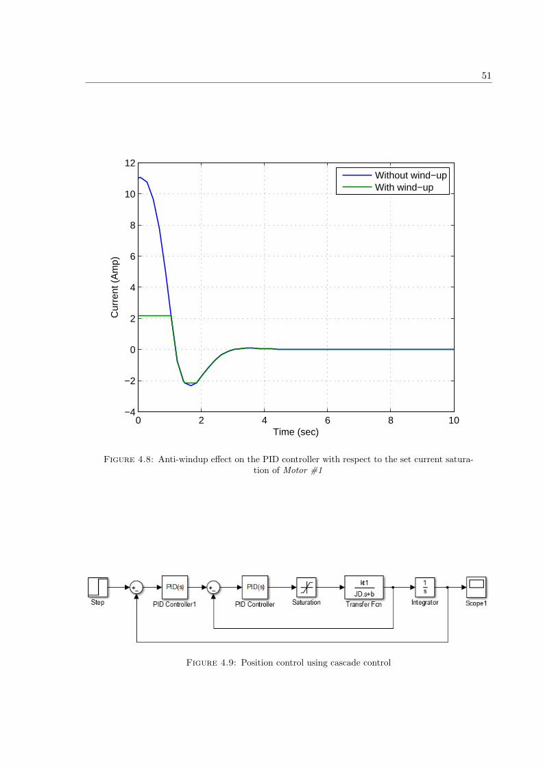
51
0 2 4 6 8 10−4
−2
0
2
4
6
8
10
12
Time (sec)
Cur
rent
(A
mp)
Without wind−upWith wind−up
Figure 4.8: Anti-windup effect on the PID controller with respect to the set current satura-tion of Motor #1
Figure 4.9: Position control using cascade control

52
0 2 4 6 8 100
0.1
0.2
0.3
0.4
0.5
0.6
0.7
0.8
0.9
1
Time (sec)
posi
tion
(rad
)
Step inputPosition of body D
Figure 4.10: Position control of body D using cascade control
0 2 4 6 8 100
0.1
0.2
0.3
0.4
0.5
0.6
0.7
0.8
0.9
1
Time (sec)
Pos
ition
(ra
d)
Step inputPosition of body C
Figure 4.11: Position control of body C using cascade control
Chapter 5
Conclusion
The objective of the thesis was to build a mathematical model of the provided commercial
four-axis control moment gyroscope and verify the validity and accuracy of the model using
laboratory experiments. The broader motivation was to demonstrate mastering of fundamental
modeling skills for electromechanical systems and prepare ground for later advanced control
design for this system, as well as for similar multi-body systems.
After giving a short technical description of the provided laboratory experimental plat-
form, the four-degree-of-freedom control moment gyroscope produced by ECP company, I
derived a set of nonlinear equations using the analytical Lagrangian method for modeling
the dynamics of the system, and provided a linearized version of the model using Taylor’s
Expansion.
As an alternative path for derivation of the model, I explored the use of a CAD platform.
Namely, I used Autodesk Inventor Professional to create a 3D model of the gyroscope and
used it to extract values of some of its physical parameters - in particular moments of inertia.
Originally, I planned to exploit the possibility to export the Simulink/Simmechanics model
directly from the CAD. This, however, turned out not a feasible solution, as the constraints
between bodies were not defined correctly.
The mathematical models were validated against data from experiments led from the
real-model. In order to make the work with the system more convenient for other future users
of the system, some hints and advices were provided for optimized use of the ECP software
environment. Additionally, some experimental maneuver provided us with useful physical
parameters of the system.
Finally, some discussion of basic control algorithms was included in the thesis, namely
PD, PID and Successive Loop Closure controls.
53


Bibliography
[1] LM13700 dual operational transconductance amplifiers with linearizing diodes and buffers,
November 1999.
[2] Eugene Butikov. Precession and nutation of a gyroscope. European Journal of Physics,
July 2006.
[3] Guojin Chen, Youping Gong, and Huipeng Chen. Modeling and simulation of loader work-
ing device based on SimMechanics. In 2011 International Conference on Transportation,
Mechanical, and Electrical Engineering (TMEE), pages 2054–2057, 2011.
[4] P. Chevrel, L. Sicot, and S. Siala. Parallel versus cascade schemes for DC-motor speed and
current control. In , Proceedings of the 36th IEEE Conference on Decision and Control,
1997, volume 1, pages 233–238 vol.1, 1997.
[5] Gene F. Franklin. Digital Control of Dynamic Systems. Ellis-Kagle Press, 3rd edition,
2006.
[6] Irving Gottlieb. Electric Motors and Control Techniques. McGraw-Hill/TAB Electronics,
2 edition, February 1994.
[7] T. R. Kane and D. A. Levinson. Dynamics: Theory and Applications. MacGraw-Hill Book
Company, 1985.
55


Appendix A
CD content
• Thesis work in PDF format
• Equations of motion of the system from Lagrangian method - MAPLE
• Linearized model from Kane’s equations - MAPLE
• CAD assembly of the control moment gyroscope - AUTODESK INVENTOR PROFES-
SIONAL
• Moments of inertia calculations using experimental data and mass properties - MATLAB
• Control effort gains measurement using experimental data - MATLAB
• Encoder gains using experimental data - MATLAB
• PD control algorithm of angular velocity of Axis #2 - ECP EXECUTIVE SOFTWARE
• PID control algorithm of angular velocity of Axis #3 - ECP EXECUTIVE SOFTWARE
• Successive loop closure of angular velocity control of Axis #4 - ECP EXECUTIVE
SOFTWARE
• Cascade control of positions of Axis #2 and Axis #3 - MATLAB
57