Modeling and control of a 4-wheel skid-steeringmobile robot: From theory to practice∗

K. Kozłowski1, D. Pazderski2 I.Rudas3, J.Tar4

Poznan University of Technology Budapest Polytechnicul. Piotrowo 3a Nepszınhaz utca 8.60-395 Poznan, Poland H-1081 Budapest, Hungary1Krzysztof.Kozlowski@put.poznan.pl 3rudas@bmf.hu2Dariusz.Pazderski@put.poznan.pl 4tar.jozsef@nik.bmf.hu

Abstract:In this paper problem of modeling and control of 4-wheel skid-steeringmobile robot is pre-sented. To obtain practical stabilization for both admissible and non-admissible trajectories[13, 7, 8], i.e. trajectories which do not satisfy nonholonomic constraint,control schemewhich is based on kinematic algorithm [4, 5] is proposed. Theoretical considerations areverified by numerical simulation and experiments. In addition some details concerning im-plementation of proposed algorithm is given.

1 Introduction

Skid-steering mobile robots (SSMRs)

Figure 1: Experimental skid-steering mobile robot

are quite different from classical wheeled mo-bile robots for which lack of slippage is usu-ally supposed – see for example [3]. In addi-tion interaction between ground and wheelsmakes their mathematical model to be uncer-tain and caused control problem to be dif-ficult as it generally demands quite detailedconsideration of dynamic properties.

In this paper we propose to use a continuousand time-differentiable control law which isbased on kinematic oscillator [5] to resolveboth regulation and trajectory tracking prob-lem. Here we refer to work done by Caracci-olo et al. [2] and our previous research whichcan be found in [10, 13]. To illustrate performance of the controller numerical simu-

∗This research was supported by the Polish-Hungarian Bilateral Technology Co-operation Project andstatuary grant No. DS 93/121/04 of Poznan University of Technology.

lations are presented. Next, experimental verification using small four-wheel SSMR(see Fig. 1) is described and some results of experiments aregiven.

2 Model of the robot

2.1 Introduction

In this section kinematic and dynamic model of four-wheel skid-steering mobilerobot is presented. We refer to the real experimental construction consists of two-wheel differentially driven mobile robots namely MiniTracker 3 (see Fig.1) [9].

In order to simplify the mathematical model of SSMR we assumethat [2]

• plane motion is considered only,

• achievable linear and angular velocities of the robot are relatively small,

• wheel contacts with surface at geometrical point (tire deformation is neglected),

• vertical forces acting on wheels are statically dependent on weight of the ve-hicle,

• viscous friction phenomenon is assumed to be negligible.

2.2 Kinematics

Firstly, consider a vehicle moving on two dimensional planewith inertial coordi-nate frame(Xg, Yg) as depicted in Fig. 1(a). To describe motion of the robot it isconvenient to define an local frame attached to it with originin its center of mass

(COM). Assume thatq ,[

X Y θ]T

∈ R3 denotes generalized coordinates,

whereX, Y determine COM position andθ is an orientation the local frame withrespect to the inertial frame, respectively.

Let v ,[

vx vy

]T∈ R

2 be a velocity vector of COM expressed in the localframe withvx andvy determining longitudinal and lateral velocity of the vehicle[4].

From Fig. 1(a) it is easy to derive kinematic equation of motion using rotation matrixas follows

q =

X

Y

θ

=

cos θ − sin θ 0sin θ cos θ 0

0 0 1

vx

vy

ω

, (1)

whereq ∈ R3 is the generalized velocity vector andω denotes angular velocity of

the vehicle.

(a) Free-body kinematics (b) Wheel velocitiesrelationships

Figure 2: Kinematics of SSMR

To complete kinematic model of SSMR additional velocity constraints should beconsidered with respect to the inertial frame. According togeometrical situationpresented in Fig. 1(b) one can prove that coordinates of velocities of pointsP1,P2,...,P4 where the wheels of the robot touch the plane must satisfy [13, 12]

vL , v1x = v2x, vR , v3x = v4x,

vF , v2y = v3y, vB , v1y = v4y,(2)

wherevL, vR denote longitudinal coordinates of left and right wheel velocities,vF

andvB , are lateral coordinates of velocities of front and rear wheels, respectively.

Remark 1 From Fig. 1(b) it is clear [13, 12] thatviy is equal to zero for straightmotion only (i.e. ifω = 0), otherwiseviy 6= 0 that implies lateral skid that isnecessary to change orientation of such vehicle.

Notice thatωL andωR which denote angular velocities of left and right wheels,respectively, can be regarded as control inputs at kinematic level and can be used tocontrol longitudinal and angular velocity according to thefollowing relationships

vx = rωL + ωR

2, ω = r

−ωL + ωR

2c, (3)

while r is so called effective radius of wheels [11] and2c is a spacing wheel trackdepicted in Fig. 1(a).

Remark 2 It is very important to note that equations (3) are valid onlyif longitu-dinal slip does not appear, otherwise they should be treatedas just approximationsand to improve accuracy parametersc andr should be identified experimentally.

Next, lateral velocityvy which determines velocity of lateral slip of the vehicle canbe obtained as follows [13]

vy + xICRω = 0, (4)

wherexICR is a coordinate of instantaneous center of rotation (ICR) ofthe robotexpressed alongxl axis. It can be proved that this equation in not integrable, henceit describes nonholonomic constraint and can be written in Pfaffian form as

[

− sin θ cos θ xICR

] [

X Y θ]T

= A (q) q = 0, (5)

where equation (1) has been used. Since the generalized velocity q is always in thenull space ofA one can write that

q = S (q) η, (6)

whereη ∈ R2 is a control input at kinematic level defined as

η ,[

vx ω]T

, (7)

S ∈ R3×2 is the following matrix

S (q) =

cos θ xICR sin θsin θ −xICR cos θ

0 1

(8)

which satisfiesST (q) AT (q) = 0. (9)

Remark 3 Equation (6) describes kinematics of SSMR which will be usedto formu-late control law. Sincedim (η) < dim (q) SSMR can be regarded as an underac-tuated system. Furthermore, because of constraint (5) thissystem is nonholonomic.

2.3 Dynamics

Figure 3: Forces and torques

Because of interaction between wheels andground dynamic properties of SSMR play avery important role. It should be noted thatif the robot is changing its orientation reac-tive friction forces are usually much higherthan forces resulting from inertia. As a con-sequence, even for relatively low velocities,dynamic properties of SSMR influence mo-tion much more than for other vehicles forwhich non-slipping and pure rolling assump-tion may be satisfied.

However in this section only simplified dy-namics of SSMR [2], which will be useful forcontrol purpose, are introduced. In order tosimplify this model we assume that the massdistribution of the vehicle is almost homogeneous, kineticenergy of the wheels and

drives can be neglected and detailed description of tyre which can be found, forexample, in [11] are omitted.

A dynamic equation of SSMR can be obtained using Euler-Lagrange principle withLagrange multipliers to include nonholonomic constraint and it can be written as

M (q) q + R (q) = B (q) τ + AT (q) λ, (10)

whereM ∈ R3×3 denotes the constant, diagonal, positive definite inertia matrix

M =

m 0 00 m 00 0 I

, (11)

m, I represent the mass and inertia, respectively,R (q) ∈ R3 denotes vector of

resultant reactive forcesFl, Fs and torqueMr

R (q) =

Fs (q) cos θ − Fl (q) sin θFs (q) sin θ + Fl (q) cos θ

Mr (q)

, (12)

B ∈ R3×2 denotes input matrix and is explicitly defined as follows

B (q) =1

r

cos θ cos θsin θ sin θ−c c

. (13)

The termτ =[

τL τR

]T∈ R

2 which appears in (10) can be treated as a controlsignal at dynamic level and represents torques generated byactuators on the left andright side of the robot. Notice that these torques produce active forcesFi (see Fig. 3)that are theoretically independent on longitudinal slip.

The reactive forces and torque in (12) are calculated as

Fs (q) =4

∑

i=1

Fsi (q) , Fl (q) =4

∑

i=1

Fli (q) (14)

and

Mr (q) = b [Fl2 (q) + Fl3 (q)] − a [Fl1 (q) + Fl4 (q)]

+c [−Fs1 (q) − Fs2 (q) + Fs3 (q) + Fs4 (q)] (15)

whereFsi (q) , µsiNi sgn (vix) , Fli (q) , µliNi sgn (viy) (16)

whileµsi andµli are dry friction coefficients forith wheel in longitudinal and lateraldirection, respectively,Ni is a reactive vertical force which acts on wheel and issupposed to be statically dependent on weight of the vehicle(see [2]).

For control purpose it would be convenient to express dynamic equation inη andη

terms. According to it one can obtain that

Mη + Cη + R = Bτ , (17)

where relationships (6) and (9) have been used,

M = ST MS, C = ST MS, R = ST R, B = ST B. (18)

3 Controller

3.1 Operational constraint

In previous section the constraint (4) was considered. However it is difficult tomeasure or estimatexICR value in practice. Therefore motivated by work done byCaraccioloet al. [2] we put an artificial constraint based on (4) and assume thatxICR = x0 = const. It can be written as

vy + x0ω = 0, (19)

wherex0 ∈ (−a, b), whilea andb are geometrical parameters depicted in Fig. 1(a).This assumption is consequently used in control development and can be interpretedas an outer-loop term in the controller which limits skid of the vehicle in lateraldirection [13].

3.2 Control objective

For control purposes the following tracking error is defined

q (t) ,[

X (t) Y (t) θ (t)]T

= q (t) − qr (t) , (20)

whereqr (t) =[

Xr (t) Yr (t) θr (t)]T

denotes reference position and orien-tation. We assume that for all times reference vector and itsfirst and second timederivative are bounded, i.e.qr (t) , qr (t) , qr (t) ∈ L∞. Here we do not imposedany additional restriction on reference signalqr (regulation case can be considered,too). Additionally, in opposite to the previous works [5, 4,10, 13] we consider thecase for whichqr is defined in a such way that velocities associated with it do notsatisfy nonholonomic constraints.

In order to facilitate subsequent control we determine kinematic error assuming thatthe constraint (19) is satisfied. Next, taking the time derivative of equation (6) andusing relationship (9) one can conclude that

˙q (t) = S (q) η − qr (t) . (21)

3.3 Position and velocity transformations

Kinematic controller based on Dixon’s scheme uses transformation which trans-forms original system – in this case described by equation (21) – to an auxiliarysystem (22) similar to nonholonomic Brockett’s integrator[1]

w = uT JT z + f, z = u, (22)

where variablesw ∈ R1 andz ∈ R

2 form three-dimensional state vector,u ∈ R2 is

a new velocity control vector andf ∈ R1 is a drift of the system, whileJ represents

a constant, skew symmetric matrix defined as

J =

[

0 −11 0

]

. (23)

It can be proved that following transformation defines global diffeomorphism withrespect to the origin

Z ,[

w zT]T

= P(

θ, θ)

q, (24)

where

P(

θ, θ)

=

−θ cos θ + 2 sin θ p12 = −θ sin θ − 2 cos θ −2x0

0 0 1cos θ sin θ 0

. (25)

Using this transformation and calculating auxiliary errors we can find velocity trans-formation which relates velocity vectorη with control signalu as follows

η = T (q, q) u + Π, (26)

where

T (q, q) =

[

L 11 0

]

(27)

is an invertible velocity transformation matrix,L = X sin θ − Y cos θ and

Π (q, qr, t) =

[

ωrL + Xr cos θ + Yr sin θωr

]

(28)

is a time-varying vector associated with reference trajectory. In the similar way wecan calculate drift termf as follows

f = 2[

ωr

(

x0 + z2 − Xr sin θ + Yr cos θ)]

. (29)

Summarizing, the obtained velocity transformation allowsto use kinematic con-troller to resolve practical stabilization for admissibleand non-admissible trajecto-ries.

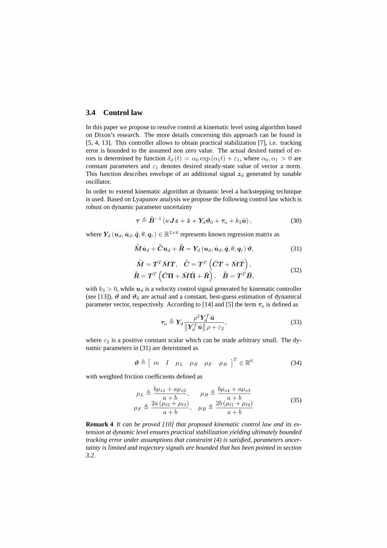
3.4 Control law

In this paper we propose to resolve control at kinematic level using algorithm basedon Dixon’s research. The more details concerning this approach can be found in[5, 4, 13]. This controller allows to obtain practical stabilization [7], i.e. trackingerror is bounded to the assumed non zero value. The actual desired tunnel of er-rors is determined by functionδd (t) = α0 exp (α1t) + ε1, whereα0, α1 > 0 areconstant parameters andε1 denotes desired steady-state value of vectorz norm.This function describes envelope of an additional signalzd generated by tunableoscillator.

In order to extend kinematic algorithm at dynamic level a backstepping techniqueis used. Based on Lyapunov analysis we propose the followingcontrol law which isrobust on dynamic parameter uncertainty

τ , ¯B−1 (wJz + z + Ydϑ0 + τa + k3u) , (30)

whereYd (ud, ud, q, θ, qr) ∈ R2×6 represents known regression matrix as

¯Mud + ¯Cud + ¯R = Yd (ud, ud, q, θ, qr) ϑ, (31)

¯M = T T MT , ¯C = T T(

CT + MT)

,

¯R = T T(

CΠ + MΠ + R)

, ¯B = T T B,(32)

with k3 > 0, whileud is a velocity control signal generated by kinematic controller(see [13]),ϑ andϑ0 are actual and a constant, best-guess estimation of dynamicalparameter vector, respectively. According to [14] and [5] the termτa is defined as

τa , Yd

ρ2Y Td u

∥

∥Y Td u

∥

∥ ρ + ε2

, (33)

whereε2 is a positive constant scalar which can be made arbitrary small. The dy-namic parameters in (31) are determined as

ϑ ,[

m I µL µR µF µB

]T∈ R

6 (34)

with weighted friction coefficients defined as

µL ,bµs1 + aµs2

a + b, µR ,

bµs4 + aµs3

a + b

µF ,2a (µl2 + µl3)

a + b, µB ,

2b (µl1 + µl4)

a + b

(35)

Remark 4 It can be proved [10] that proposed kinematic control law andits ex-tension at dynamic level ensures practical stabilization yielding ultimately boundedtracking error under assumptions that constraint (4) is satisfied, parameters uncer-tainty is limited and trajectory signals are bounded that has been pointed in section3.2.

4 Simulation results

In this section we present simulation results performed in Matlab/Simulink envi-ronment to verify behavior of the controller. The parameters of the SSMR modelwere chosen to correspond as closely as possible to the real experimental robot pre-sented in section 1 in the following manner:a = b = 0.039[m], c = 0.034[m],r = 0.0265[m], m = 1[kg], I = 0.0036[kg · m2].

Permissible torque signal and angular velocities of wheelswere saturated as:τmax = 0.25[Nm], ωmax = 56[rad/s]. Friction parameters of the surfaceµsi

andµliwere modeled using scalar functions depending on actual position of centerof ith wheel expressed in the inertial frame and were supposed to bebounded asfollows: 0.02 ≤ µsi ≤ 0.18, 0.2 ≤ µli ≤ 0.8.

Remark 5 For comparison purpose initial conditions and the parameters assumedin simulations correspond to those used in experiments which are described in sec-tion 5.

Firstly, regulation problem is examined. The initial posture error was selected as

q (0) =[

0 0.5 −π/4]T

. The control gains were given ask1 = 0.5, k2 = 0.5,k3 = 10, while coefficients which determine accuracy in steady-state wereε1 =0.01 andε2 = 0.1. The oscillator signal was initialized as follows

zd (0) = 1.5[

cos (−π/3) sin (−π/3)]T

and the coefficient which determines desired convergence oferrors was selected asα1 = 0.4.

The best-guess estimates of mass and inertia were 20 and 50 percent higher, respec-tively, than parameters assumed for the robot model. Next, estimates of frictioncoefficients were selected asµL0 = µR0 = 0.1 andµF0 = µB0 = 0.5, whilebounding coefficientρ = 1. Furthermore, the constantx0 related to ICR positionwas assumed to be equal to−0.02 [m].

In Fig. 3(a) performed trajectory in Cartesian space is depicted and the position andorientation is marked at every second of simulation. From Fig. 3(b) it is clear thatinitial errors are significant reduced and in steady-state are bounded as follows

∣

∣

∣X

∣

∣

∣< 5[mm],

∣

∣

∣Y

∣

∣

∣< 5[mm],

∣

∣

∣θ∣

∣

∣< 0.01[rad].

It is worth to note that convergence to the set of permissibleerrors is exponential.

In the next simulation trajectory tracking were examined. The sinusoidal admissiblereference trajectory were selected as

Xr = 0.1t [m] , Yr = 0.3 sin (0.6t) [m] ,

while θr was numerically calculated to satisfy the constraint (19).The initial oscil-lator signal was selected as

zd (0) = 0.4[

cos (−π/2) sin (−π/2)]T

−0.6 −0.4 −0.2 0 0.2 0.4−0.1

0

0.1

0.2

0.3

0.4

0.5

0.6

X [m]

Y [m

]

q(t)q

r(t)

q(0)q

r(0)

(a) Performed trajectory

0 5 10 15 20−1.5

−1

−0.5

0

0.5

1

time [s]

X−

Xr [m

], Y

−Y

r [m],

θ−θ r [r

ad] X−X

rY−Y

rθ−θ

r

(b) Regulation errors

Figure 4: Regulation case

and the gain coefficientk2 was increased to 1 in comparison to the previous simu-lation. Other parameters of the controller remained unchanged.

−0.5 0 0.5 1 1.5 2 2.5−0.4

−0.2

0

0.2

0.4

0.6

X [m]

Y [m

]

q(t)q

r(t)

q(0)q

r(0)

(a) Performed and reference trajectory

0 5 10 15 20−0.6

−0.4

−0.2

0

0.2

0.4

time [s]

X−

Xr [m

], Y

−Y

r [m],

θ−θ r [r

ad] X−X

rY−Y

rθ−θ

r

(b) Regulation errors

Figure 5: Admissible trajectory case

The reference and performed trajectory are presented in Fig. 4(a) using stroboscopicview, while position and orientation errors are depicted inFig. 4(b). These steady-state errors are bounded as

∣

∣

∣X

∣

∣

∣< 10[mm],

∣

∣

∣Y

∣

∣

∣< 10[mm],

∣

∣

∣θ∣

∣

∣< 0.01[rad].

It should be noted that further error reduction in steady-state is possible by choosingsmaller valueε1. Next, convergence of errors may be improved by increasing valueα1. However, tuning of the controller parameters should take into considerationlimitation of torque and velocity signals since forcing toosmall desired errors ortoo fast convergence may result in bad performance of the controller and may causechattering phenomenon.

5 Experimental verification

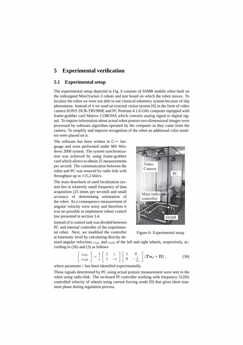
5.1 Experimental setup

The experimental setup depicted in Fig. 6 consists of SSMR mobile robot built onthe redesigned MiniTracker-3 robots and test board on whichthe robot moves. Tolocalize the robot we were not able to use classical odometrysystem because of slipphenomena. Instead of it we used an external vision system [6] in the form of videocamera SONY DCR-TRV900E and PC Pentium 4 1.6 GHz computer equipped withframe-grabber card Matrox CORONA which converts analog signal to digital sig-nal. To inquire information about actual robot posture two-dimensional images wereprocessed by software algorithm operated by the computer asthey came from thecamera. To simplify and improve recognition of the robot an additional color mark-ers were placed on it.

The software has been written in C++ lan-

Figure 6: Experimental setup

guage and were performed under MS Win-dows 2000 system. The system synchroniza-tion was achieved by using frame-grabbercard which allows to obtain 25 measurementsper second. The communication between therobot and PC was ensured by radio link withthroughput up to 115,2 kbit/s.

The main drawback of used localization sys-tem lies in relatively small frequency of dataacquisition (25 times per second) and smallaccuracy of determining orientation ofthe robot. As a consequence measurement ofangular velocity were noisy and therefore itwas no possible to implement robust controllaw presented in section 3.4.

Instead of it control task was divided betweenPC and internal controller of the experimen-tal robot. Next, we modified the controllerat kinematic level by calculating directly de-sired angular velocitiesωdL andωdR of the left and right wheels, respectively, ac-cording to (26) and (3) as follows

[

ωdL

ωdR

]

=1

r

[

1 c1 −c

] [

1 00 − 1

x0

]

(Tud + Π) , (36)

where parameterc has been identified experimentally.

These signals determined by PC using actual posture measurement were sent to therobot using radio-link. The on-board PI controller workingwith frequency 512Hzcontrolled velocity of wheels using current forcing mode [9] that gives short tran-sient phase during regulation process.

To calculate oscillator signalzd trapezoidal integration routine was used. In additionto ensure numerical stability of the algorithm scaling operation was performed tostabilized envelope of‖zd‖ determined by functionδd (t).

Figure 7: Controller diagram

Remark 6 It should be noted that implemented control scheme is based on assump-tion that longitudinal slip is negligible. In theory this assumption would not benecessary for overall controller previously verified in simulation section.

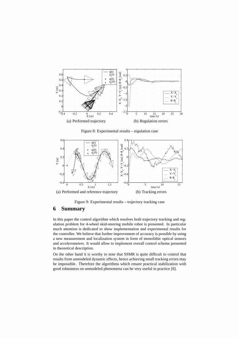
5.2 Results

To validate the proposed simplified algorithm results of experiments are presented.

Firstly, we considered the regulation problem, i.e. parking problem. The parametersof the controller and initial conditions were presented in section 4, howeverε1 wasincreased to0.05 to ensure better robustness and less sensitiveness to measurementnoise.

The results are depicted in Figs. 7(a)–7(b). From Fig. 7(a) one can see that steady-states position and orientation errors were bounded as follows

∣

∣

∣X

∣

∣

∣< 20[mm],

∣

∣

∣Y

∣

∣

∣< 20[mm],

∣

∣

∣θ∣

∣

∣< 0.03[rad].

In the next experiment trajectory tracking was verified. Thereference trajectory wasthe same as it used in simulation and the parameterε1 was selected asε1 = 0.15to improve robustness of the controller. From Fig. 8(a) and 8(b) one can see thataccuracy of tracking is significantly less than accuracy obtained for regulation thatresults mainly from unmodeled dynamic effects (for exampleslip phenomenon) anddelays in the control loop. The tracking errors were boundedas

∣

∣

∣X

∣

∣

∣< 80[mm],

∣

∣

∣Y

∣

∣

∣< 180[mm],

∣

∣

∣θ∣

∣

∣< 0.3[rad].

−0.4 −0.2 0 0.2 0.4−0.1

0

0.1

0.2

0.3

0.4

0.5

0.6

X [m]

Y [m

]

q(t)q

r(t)

q(0)q

r(0)

(a) Performed trajectory

0 5 10 15 20 25 30−2.5

−2

−1.5

−1

−0.5

0

0.5

1

time [s]X

−X

r, Y−

Yr [m

]; θ−

θ r [rad

]

X−Xr

Y−Yr

θ−θr

(b) Regulation errors

Figure 8: Experimental results – regulation case

0 0.5 1 1.5−0.4

−0.2

0

0.2

0.4

0.6

X [m]

Y [m

]

q(t)q

r(t)

q(0)q

r(0)

(a) Performed and reference trajectory

0 5 10 15−0.6

−0.4

−0.2

0

0.2

0.4

time [s]

X−

Xr, Y

−Y

r [m];

θ−θ r [r

ad]

X−Xr

Y−Yr

θ−θr

(b) Tracking errors

Figure 9: Experimental results – trajectory tracking case

6 Summary

In this paper the control algorithm which resolves both trajectory tracking and reg-ulation problem for 4-wheel skid-steering mobile robot is presented. In particularmuch attention is dedicated to show implementation and experimental results forthe controller. We believe that further improvement of accuracy is possible by usinga new measurement and localization system in form of monolithic optical sensorsand accelerometers. It would allow to implement overall control scheme presentedin theoretical description.

On the other hand it is worthy to note that SSMR is quite difficult to control thatresults from unmodeled dynamic effects, hence achieving small tracking errors maybe impossible. Therefore the algorithms which ensure practical stabilization withgood robustness on unmodeled phenomena can be very useful inpractice [8].

References

[1] R. W. Brockett, “Asymptotic stability and feedback stabilization”,Differential Geo-metric Control Theoryedited by R. W. Brockett, R. S. Milman and H. J. Susmann,Birkhauser, Boston, pp. 181-191, 1983.

[2] L. Caracciolo, A. De Luca, S. Iannitti, “Trajectory tracking controlof a four-wheel dif-ferentially driven mobile robot”,IEEE Int. Conf. on Robotics and Automation, Detroit,MI, pp. 2632-2638, May 1999.

[3] G. Campion, G. Bastin, B. DAndrea-Novel, “Structural Propertiesand Classification ofKinematic and Dynamic Models of Wheeled Mobile Robots”,IEEE Transactions onRobotics and Automation, Vol. 12, No.1, pp. 47-62, February 1996.

[4] W.E.Dixon, A.Behal, D.M.Dawson, S.P.Nagarkatti,Nonlinear Control of EngineeringSystems, A Lyapunov-Based Approach, Birkhauser 2003.

[5] W. E. Dixon, D. M. Dawson, E. Zergeroglu and A. Behal,Nonlinear Control ofWheeled Mobile Robots, Springer-Verlag, 2001.

[6] P. Dutkiewicz, M. Kiełczewski, “Vision feedback in control of a group of mobilerobots”. Proc. of theSeventh International Conference on Climbing and WalkingRobots and their Supporting Technologies for Mobile Machines CLAWAR 2004, Madrit2004 (to appear).

[7] P. Morin, C. Samson, “Practical Stabilization of Driftless Systems on Lie Groups: TheTransverse Function Approach”,IEEE Transactions on Automatic Control, Vol. 48,No.9, pp.1496-1508, September 2003.

[8] P. Morin, C. Samson, “Feedback control of nonholonomic wheeled vehicles, A survey”,Archives of Control Sciences, Vol. 12, pp.7-36, 2002.

[9] T. Jedwabny, M. Kowalski, M. Kiełczewski, M. Ławniczak, M. Michalski,M. Michałek, D. Pazderski, K. Kozłowski, Nonholonomic mobile robot MiniTracker 3for research and educational purposes,35

th International Symposium on Robotics,Paris 2004.

[10] K. Kozłowski, D. Pazderski, “Control of a Four-Wheel Vehicle Using Kinematic Os-cillator”. Proc. of theSixth International Conference on Climbing and Walking Robotsand their Supporting Technologies CLAWAR 2003, pp. 135-146, Catania 2003.

[11] H. B. Pacejka,Tyre and Vehicle Dynamics, Butterworth-Heinemann, 2002.

[12] D. Pazderski, K. Kozłowski, M. Ławniczak, “Practical stabilizationof 4WD skid-steering mobile robot”. Proc. of theFourth International Workshop on Robot Motionand Control, Puszczykowo, pp. 175-180, 2004.

[13] D.Pazderski, K.Kozłowski, W.E.Dixon, “Tracking and Regulation Control of a SkidSteering Vehicle”,American Nuclear Society Tenth International Topical Meeting onRobotics and Remote Systems, Gainesville, Florida, pp. 369-376, March 28-April 12004.

[14] M. W. Spong, “On the Robust Control of Robot Manipulators”,IEEE Transactions onAutomatic Control, Volume 37, No. 11, pp. 1782-1786, November 1992.