modeling analysis and simulation(1)

7/28/2019 Modeling Analysis and Simulation(1)

http://slidepdf.com/reader/full/modeling-analysis-and-simulation1 1/19

STIRRED TANK HEATERS MOD UL E

5

Afíer sludying this module, the reader shoukl be able to:

• Develop the nontinear dynamic modcl of a pert'eetly mixed stirred lank healer• Find the slale-space and transter funclion form oí a línearízed stirred Lank heater• Compare the dynamic respoases of the nonlinear and linear models• Use MATLAB for linear and nonlinear simulations• A nalyze phase-planc behavior

The major sections in this module are:

M5..I IntroductionM'5,2 Developing the Dynamic ModclM5.3 Sleady-State ConditionsM5.4 Slate-Space ModclM5.5 Laplace Domain ModelM5.6 Step Responscs: L inear versus Nonlinear íVIodelsM5.7 Unforced Systcm Responses: Perturbalions in Initial Conditions

M5.1 INTRODUCTION

Mixing vessels are used in many chemical processes. Oten íhese mixing vessels areheated, eilher by a coi! or a jackct surrounding the vessei. For cxampíe, a mixing vesselmay serve as a chemical reactor, wherc tvvo or more eomponents are reaeted to produce

471



472 S tirred T ank H eaters M oduí e 5

Tank F¡

inlet T¡

Jacket F¡ouítet T¡

J acket inlet F¡¡ T¡¡

Tank outlel

F r

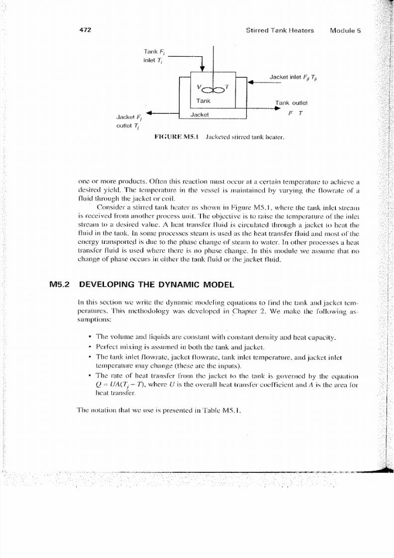
1TGURE IVI5.1 jackeled stirred tnnk heater.

onc or more producís. Oflen thís reaction musí oecur at a ccrtain temperatura to achieve adesired yield, Thc temperature in the vesse] is maintained by varying íhe flowrate of afluid ihrough the jacket or coi!.

Consider a stirred tank heater as shown in Figure M5.1, wItere the tank iníel slreamis received i'roin another process unil. The objective is lo rai.se thc icmpcralure of the ¡nielslream lo a desired valué. A heaí. transfer Huid is cireulaled through a jaekel lo heal thefluid in íhe tank. In some processes steam is used as ihe heat. transfer fluid and most ol'thccnergy transponed is due to thc phase ehange of" steam to walcr. In other processes a heaítransl'er fluid is used where thcre is no phase change. In this module we assume ihat noehange of phase oectirs in cither the tank fluid or the jacket fluid.

M5.2 DEVELOPING THE DY NA MIC MODEL

In thís seetion we wrile íhe dynamic modeling equalíons to 11 nd the tank and jaekel tem~peratures. This methodology was developed in Chapter 2. We makc íhe foliowing as-sumpíions:

• The volunte and liqítids are constant with constant density and heat capacily.• Pcrfeet mixing j.s assumed in both the lank and jacket.• The tank inlet flowrate, jacket flowrate, tank inlet temperature, and jacket inlet

temperattire may change (these are the itiputs).• The rate of heat transl'er from thc jacket to íhe lank is governed by the eqiiation

Q = UA(Tj - 7), where U is the overal! heat transfer coefl'icient and A is the área forheat transfer.

The notalion that wc use is presenled ín Table M5.1.

http://rai.se/

http://rai.se/

http://rai.se/



S ec. M5.2 D eveloping the D ynamic Model 473

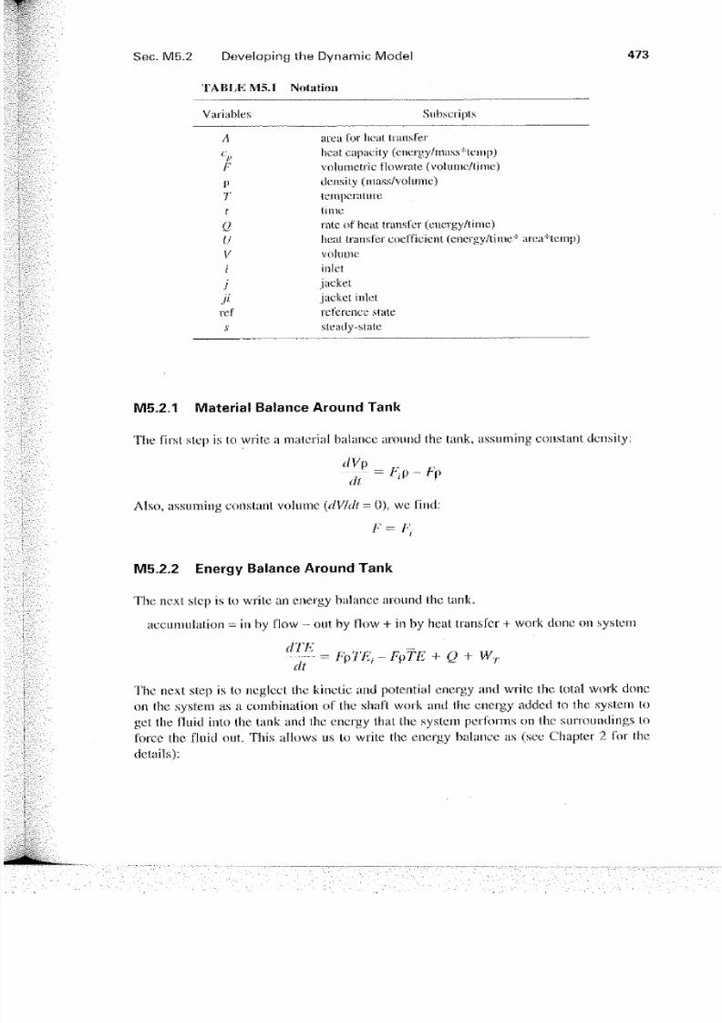
T Mil Ai M5.1 Notation

Variables

Act,Fí>Tt

üI JVi

jjiref

.V

Subscripls

área Cor lieat transferlieat capacity {energy/mass*lemp)

volumetric flowrate (voliime/üme)ilensily (mass/volume)tenipcraturetimeinte of hcat transfer (aievgy/ti mc)lieat transfer coefficíent (energy/tinie* arca*tcmp)vohitneinlet¡aeketjackel inletret'erenee state

steady-slate

IVI5.2.1 M aterial Balance A round T ank

The first step is to write a material balance around the tank, assuming constant dcnsity:

- ¿ T - ^p - í p

AI so, assuming constant volume (dV/dt= 0), wc find:

M5.2.2 E nergy Balance A round T ank

The ncxt slcp is to write an energy balance around the tank.

accumulafion = in by .flow - out by flow + in by heat transfer + work done 011 system

--■-■■= F9W

i-F

i,TE+Q+ W

TdtThe next step is to negicct the kinctic and potential energy and vvritc the total work doneon the .system as a combination oí the shaft vvork and the cnergy added to the system toget the Huid hito the tank and the energy that the system petforms on the surroundings toforcé the fluid out. This allows us lo write the energy balance as (see Chapter 2 íbr thedetails):



474 S tirred T ank H eaters M odule 5

f-rpfa + ^ -^ + ^ + Q + w,

and since H= U +pV, we can. rewríte the energy balance as:

dll dpV

" í ¿ . . - - £ . . = f p / / . _ . / . p / / + Q+W,

Note (has dpVIdt = V dpldt +p dV/dt, and the voiume is constant. Also, the mean pressurechange can be negiccted since the density is constant:

dll- = Fp II, - Fp II + Q + Wr

Neglccting the work done by the mixing impcflcr, and assuming single phase and a constant heat capacily, we find:

We musí also perform a material and energy balance around the jacket and use íhe con-necting relationship for heat transfer between the jacket and the tank.

M5.2.3 M aterial Balance A roun d the J acket

The material balance around the jacket is (assuming constant density):

dVM - F r

assuming constant voiume (dVIdt - 0), we find:

F F̂¡t

M5.2.4 E nergy Balance A round the J acket

Next, we wrile an energy balance around the jacket. M aking the same assumptions asaround the tank:

di) F , O

We also havc the relationship Cor heat transfer frorn the ¡acket to the tank:



S ec. M5.4 S íate-S pace Model 475

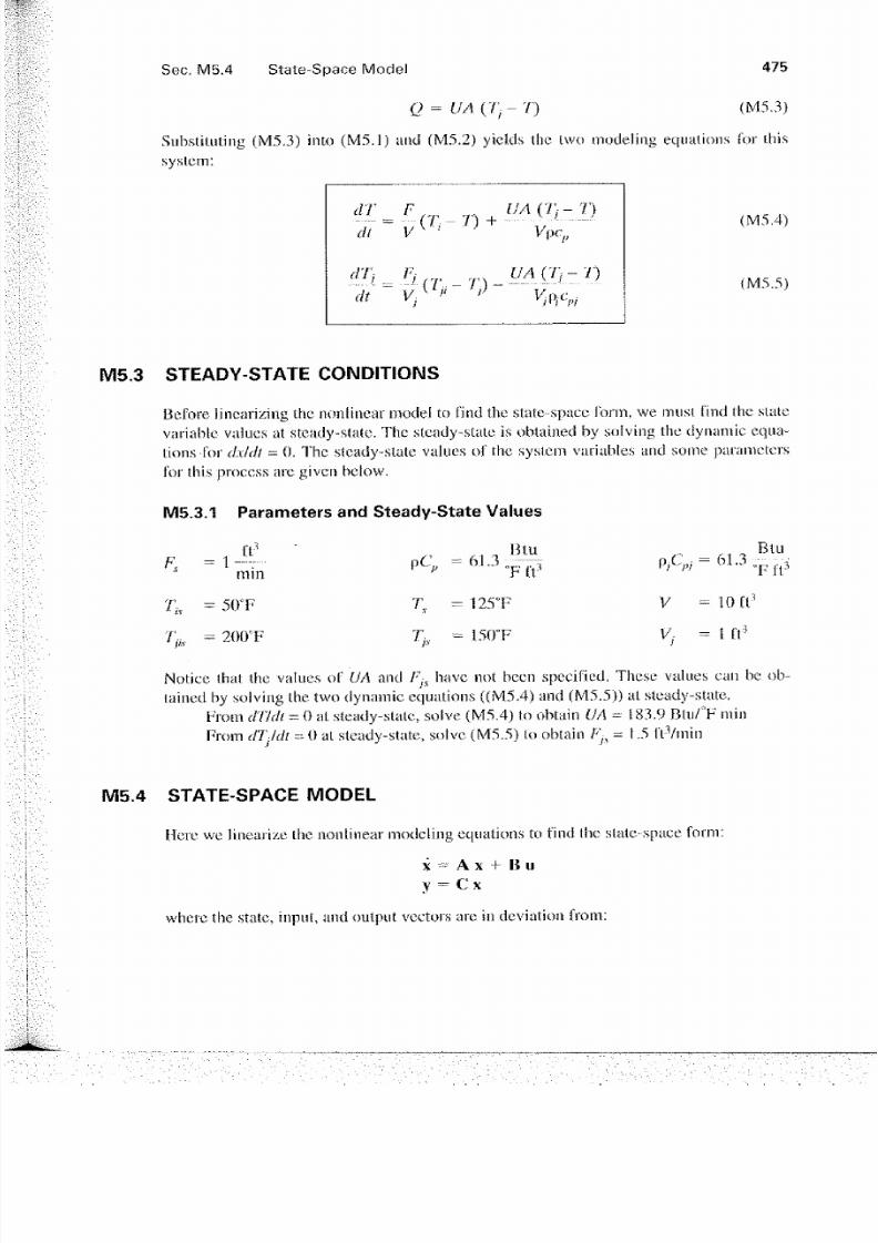
Q = VA (7} - 7) (M5.3)

SubstiU iting (M 5.3) into (M5.1) anci (M5.2) yieids thc lwo modeling equations for thissysiem:

(M5.4)lTdt

dt

" > .

= v^ÍM (7} -7 ' )

<M5.5)

M5.3 S TE ADY -S TAT E CONDIT IONS

Before lincarizing thc nonlinear modei to find the statc-spacc ibnn, we musí find the slatevariable vaiues at steudy-slaíe. Thc steady-state is obtained by sofving the dynaniic equations-for dxldt = 0. The síeady-stale valúes of thc sysiem variables und some panmietersfor this process are given below.

M5.3.1 Parameters and Steady -State Valúes

= 1 irmuí

= 50T

= 200°F

Pc,

T,

T-

= 61.3 T

T rt'

= Í25T= 1.50T

, , o B t L 1

V =10 Et3

V : Í r t5

Notice that the valúes of (J A and F js have not becn speeified. Thcse vaiues can be obtained by solving the two dynamic equations {(M5.4) and (M5.5)) at steady-state.

From dTIdi =0 at steady-state, sol ve (M5.4) to obtain (JA = 183,9 Btu/°F minFrom dT-ldl = 0 at steady-state, solve (M 5.5) to obtain Fyí = 1.5 IVVmin

M5.4 S TATE -SP ACE MODE L

Mere we linearize the nonlinear modeling equations to find the slate-space form:

x ~ A x + B uV = C x

where the state, input, and output vectora are in deviation from:



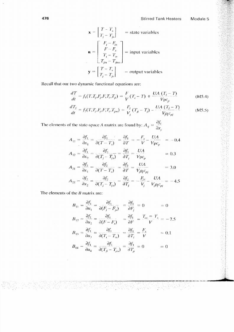
476 S tirred T ank H eaters Modul

x -

y =

F-F s

- fin ¡inx-

T-TA

' ' )~' ti

— statc variables

input variables

outpitt variables

Rccall that ouv two dynamic functioiíai cquations are

dT

di

didt

f V

I') pj,

The elements of the state-space A matrix are í'ound by: A"' dx,

(M 5

(M5

^n =

A

3/i 3/i 3/t /*;. ÜAdxl d(T-'Q d'F V Vpcp

3/i -.. df* - dA _ UA

dx2 d{TrTjs) di) Vpcp

A = df2 <*fi = Ah = OA21 3x, 'd(T-T) ~ dT V¿p~c~

= -0.4

= 0.3

= 3.0

A ? ^ ^ = ^ = . ^ = ^ _ . ^ . = _ 4 ,('!

The elements oí" the B matiix are:

5/,o«t d(Fj~Fj,) dF j

= 0

w ,- "¿i. = " ¿\" n du2 3 ( F - / g r)/-

■7.5

u ~ dih 3(7 ; - 7 ; ) " 37 i V

B, a/i a/, y ,a«< 3('/;,.-7; i t) 37;,

= o.i

= 0



S ec. M5.5 Laplace D omain Model 477

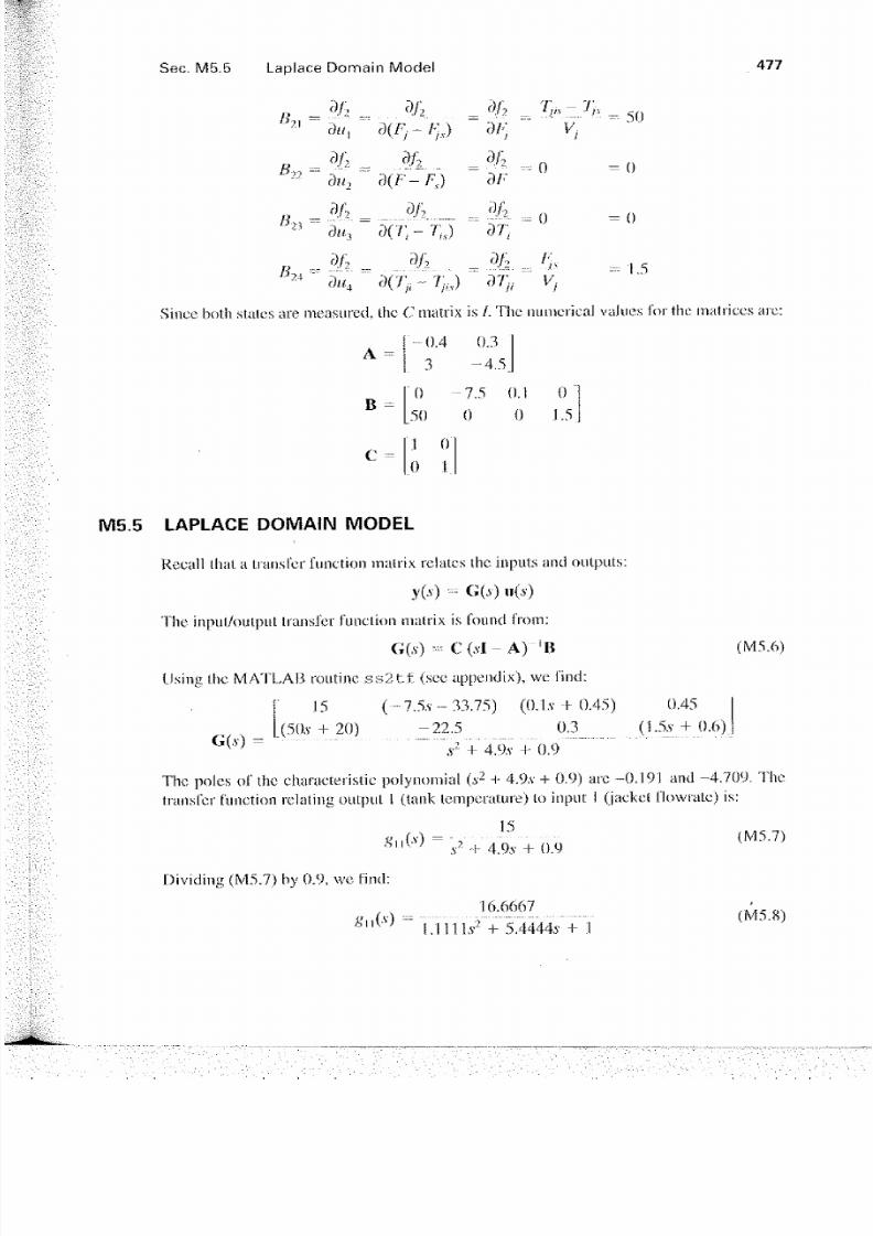
#7.1 =

B,

df2 <V2 ¥2 ... T̂ 'J),

a«, a(í}-/•;.,) a/>;

a«2 a'cF -"/:;) a/-

V:50

/ ia/' _ d/2 <%

2 Í

# 2 4 =

du3 a(?; - T;,) a? ;- o

- o

= o

d/2 aj2 df2 /<;,1.5

a«4 3 ( 7 }, - )̂ <r/;,. v¡

Since both statcs are measured, thc C matrix is /. The numerical valúes i'or the matrices are:

[ -0 .4 0.3

H 3 -4.5.

0 -7.5 0.1 0 ":50 0 0 1.5

C1 00 1

WI5.5 LAPLACE D OMA IN MODE L

Recall that a tranxfcr function matrix relates the ínputs and oulputs:

y(.v) = G(.v) 11(5)

The input/oulput tranxíer function matrix ís found í'rotn:

G(.v) - C (. vl - A ) - 'B (M5.6)

Using the ¡VIATLAR routine ss2tf (scc appendix), we i'ind:

j " 15 ( 7.5.V -33.75) (0.1.v + 0.45) 0,45 |L(50.v + 20)

G(.v)-22.5 0.:

,v2 + 4.9.v + 0.9

(1.5* + 0.6) j

The poles oí the characteristic poíynomial (s2 + 4.9.v + 0.9) are -0.191 and -4.709. The

transfer function relating outpul 1 (tank lemperature) lo itiput I (jactó ílowíate) is:15

S"('v) - ,2 + 4.9.v + 0.9

Dividing (M 5.7) by 0.9, we fincl:

£11 C v)16.6667

¡.lilis2 + 5.4444.V + 1

(M5.7)

(¡VI5.8)



478 S tirred T ank H eaters Module 5

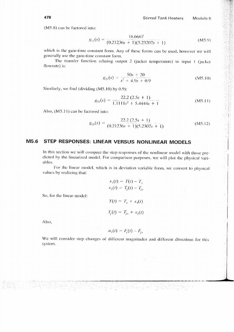
(M 5.8) can be facíored inlo:

16-6667Su(S) (Ü.21236.V +])(5.Z3207Í+Í) {M5'9)

which i.s the gain-lime conslant. form. Any of these forms can be useci, however we willgenerally use fine gain-tíme constan! form.

The transfer function rciating outpul 2 (jackeí tcmperalure) !o input I (jaekelflovvrate) is:

50.v f 20& l ( í ) = r + 4.9.7 0.9 f M 5 ' l 0 )

Similarly, we i'ind (dividíng (M 5.I0) by 0.9):

22.2 (2.5s + 1)

Al so, (M 5.11) can be faciored into:

22.2 (2.5i- + I ),!>'21

-] " (6.21.236s T Í)(5.2307.v + I.) (M 5.12)

M5.6 S T E P RE S PO NS E S : LINE A R VE R S U S NO NL INE A R MO D E LS

ín this scction we will compare the slep responsos of the nonlinear model with thosc pre-clieted by the linearized model For cornparison purpo.ses, we will plot the physical vari

ables.Por thc linear model, which is in deviation variable form, we convert to physical

valúes by realizing thal:

xi(r) = 7X0-7;x2(t) = 7}(f) - l)s

So, for the linear model:

Al so,

?■/) = /; + .v,{/)

Wc will consider slep changes of difieren! magnitudes and tiifferent directions for thi.ssystem.

■Í É



S ec. M5.6 S tep R esponses: Linear Versus N onlinear Models 479

R/15.6,1 S m a l l i n c r ea s e ín J ac k e t T e m p e r a t u r e

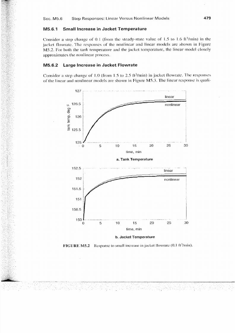
Consider a step change oí" 0.1 (írom the sleady-state valué oí l.5 to l .6 lTVmin) in thejackel flowrate. The responses oí the nonlinear and linear models are shown in FigureM5.2. For bolh ihe tatik temperature and ihc jackel temperature, the linear inociel closely

approximates the nonlinear proeess.

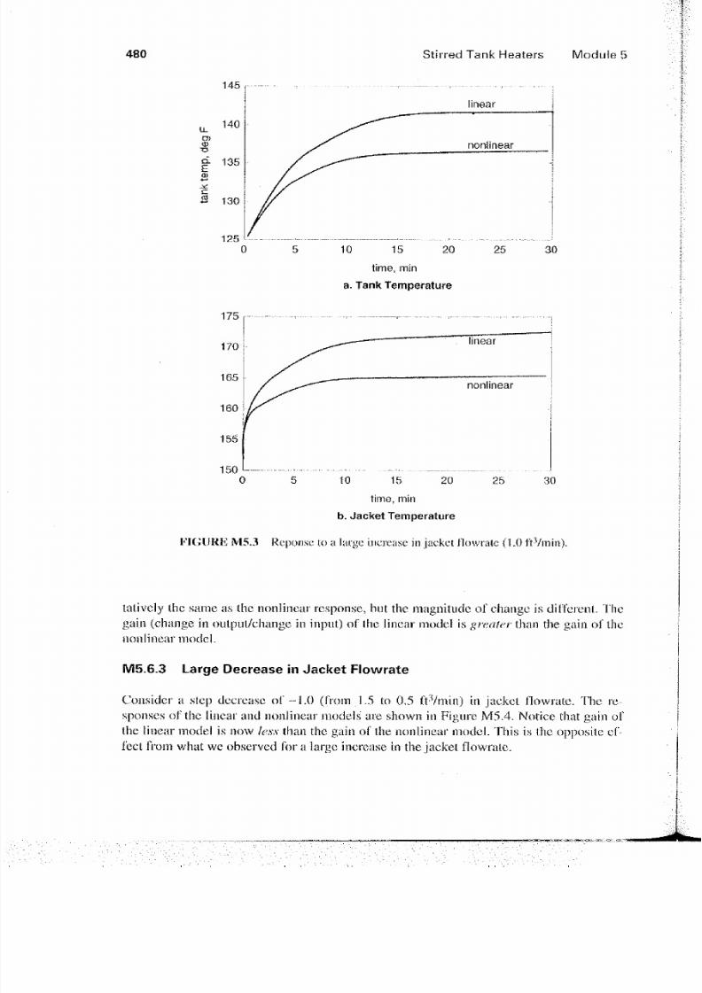
M5.6.2 Large Increase in J acket F iowrate

Consider a step ehange oí LO (írom l .5 to 2.5 ¡VVmin) in jackel Hovvrate. The i'esponsesoí the linear and nonlinear models are shown in Figure M 5.3. The linear response is quali-

12?

u- 126-5

-a§ 1260)

125.5

12510 15

time, mn

a. T ank Tempera tu re

30

150,5

10 15

time, min

30

b. Jacket Temp erature

FIGURE M5.2 ResponsoSo small incitase in jaekeí lowrute (0.1 f't-Vmin).



480 S tirred T ank H eaters M odule 5

145

140

g- 135

130

125

linear

nonanear

205

time, mín

a. Tank Temperatura

25 30

10 15 20 25 30time, min

b. Jacket Temperature

FIGURE M5.3 Rcponsc to a large ulerease in jacket flowrate (1.0ftVmm).

talively thc same as thc nonlinear responso, but the magnitude of change is different. Thegain (change in oulpul/change in inpnt) of (he linear model is greater than the gain of thenonlinear model.

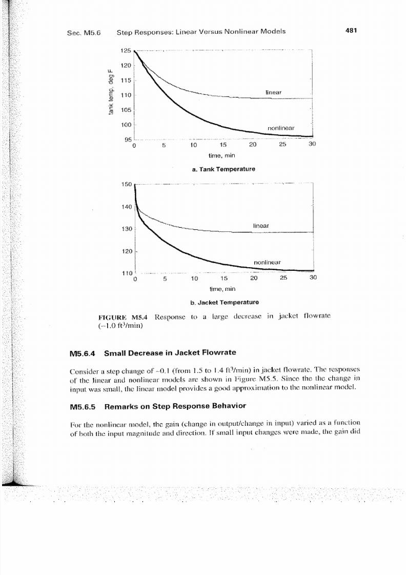
M5.6.3 Large Oecrease in J acket F lowrate

Consider a slep decrease of -1,0 (from.1.5 to 0.5 íTVmin) in jacket nowrate. The responsos of the linear and nonlinear models are shown in Figure M5.4. Notice that gain ofthe linear model is now less than the gain of tlie nonlinear model. This is the opposile ef-fecl from what we observed for a large increase in the jacket flowrate.



S ec. M5.6 S tep R esponses: Linear Versus N onünear M odels 4 8 1

1S0

140

130

120

110 '■

0

10 15

time, min

20 25

a. Tank Tem perature

5 10 15lime, min

b. Jacket Tem perature

FIGURE M5.4 Response to a large dccrease in jacket flowrate(-1.0ft3/min)

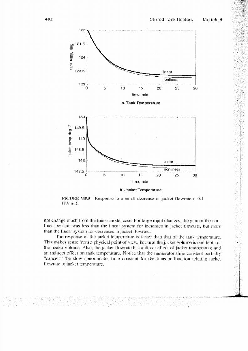
M5.6.4 S mai! D ecrease in J acket F lowrate

Consider a stcp change of -0,1 (from 1.5 to 1,4 ftVmin) in jacket flowrate. The responsesof the linear and nonlincar modeís are shown in Figure M 5.5. Since the the change ininput was small, the linear inodel provides a good approxirnation to the nonlincar model.

M5.6.5 R emarks on S tep R esponse Behavior

For the nonlincar model, the gain (change in output/change in input) vatied as a funclionof both the input raagnitude and direction. [f small input changcs were made, the gain did



4 8 2 S tirred T ank H eaters M odu le 5

125

124.5

Ií124

123.5

12310 15

¡me, min

nonlirtear

20 25 30

a. Tank Tem peratura

150

b. Jacket Temperature

FIGURE ¡V15.5 Response lo a small dccrease in jacket flowratc (-0.ft-Vmin).

not chango much from the linear model case. For large input changos, the gain of the non-

linear system was less than the linear system for increases in jacket t'iowrate, bul inorethan the linear system for decreases in jacket fíowrate.The response of the jacket temperature is iaster than that of the tank temperature.

This makes sense from a physical point of view, because the jacket volume is one-lenth ofShe heater volume. A lso, the jacket flowratc has a direct: cffect of jacket temperature andan indirect effect on tank temperature. Notice that the numerator l ime constan! partially"caneéis" the slow denominaíor time constant for .the transfer function relating jacketflowratc (o jacket temperature.



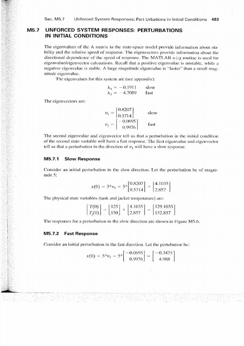
S ec. M5.7 Unforced S ystem R esponses: P ert U rbations in Initial C onditions 483

M5.7 U NFO RCE D S Y S T E M RE S PO NS E S : PE R T U RBA T IO NS!N INIT IAL CONDIT IONS

The eigenvaíues of the A matrix iit the state-space model provide information about. sta-bilily and (he relalive speed of respon.se. The eigenvectors provide information about the

directional dependence of the speed of response, The MATLAB ei g routine is useti forejgenvalue/eigenvector calcuations, Recaí! that a positive eigenvalue is unstabte, while anegativo eigenvalue is stable. A iarge magnitude eigenvalue is "fasler" than a small mag-nítude eigenvalue.

The eigenvalties for ihis system are (see appendix):

The eigenvectors are:

A , = -0.1911k2 = -4.7089

2 ~J"

0.82071

0.5714 I"-0.0695"

0.9976

slowfast

slow

fast

The second eigenvalue and eigenvector tell us that. a perturbation in the initial conditionof the second state variable will have a fast response. The first eigenvalue and eigenvectortell us that a perturbation in the direction of v] will have a slow response.

M5.7.1 S low R esponse

Consider an initial perturbation in the slow direction. L et the perturbation be of magnitude 5:

x(0) = 5*v2 = 5*0.82070.5714

4.10352.857

The physical state variables (tank and jackel temperaturc) are:

7'(0) 1.25

150

4.10352,857

129.1035152.857

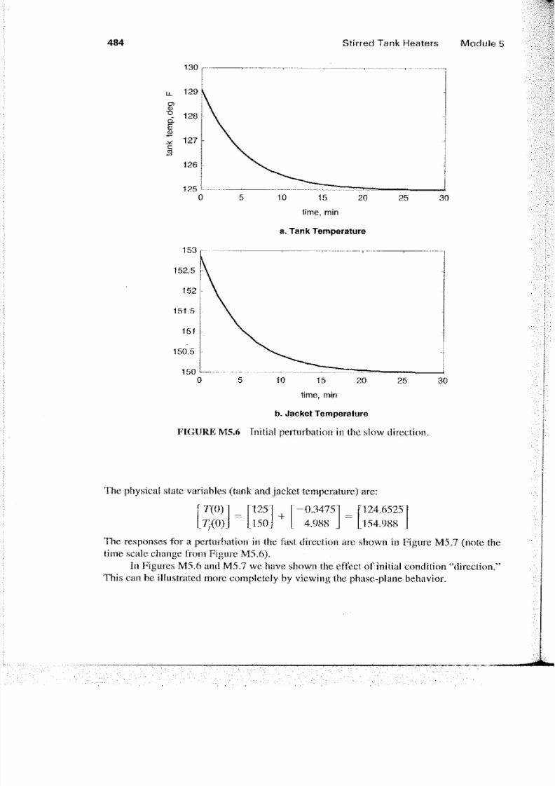
The responses for a perturbation in the slow direction are shovvn in Figure M5.6.

M5.7.2 F ast R esponse

Consider an initial perturbation. in the fast direction. L et the pertubation be:

jt({)) = 5*w2 - 5*-0.0695

0.9976

-0.34754.988

http://respon.se/

http://respon.se/

http://respon.se/



S tirred T ank H eaters Module 5

130

a. Tank Tem peratura

10 15timo, mirt

20 25 30

b. J acket Temperatura

FIGURE M5.6 Initiat perturbation in the slow direction.

The physicai state variables (tank and jacket temperatura) are:

7X0) 125150

-0.34754.988

[124.6525154.988

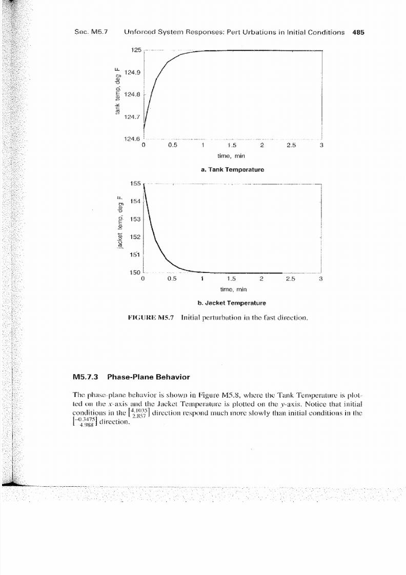
The responses for a perturbation in the fast direction are shown in Figure M5.7 (note thetime scale change from Figure M 5.6).

In Figures M5.6 and M5.7 we have shown the effcct of initial condition "direclion,"This can be iüustrated more completely by viewing the phase-plane behavior.



S ec. M5.7 Unforced S ystem R esponses: P ert Urbations ¡n Initíal C onditions 485

125

124.6

155

a"O

£

2.5

a. Tank Temperatura

1.5 2 2.5time, m¡r¡

ü. J acket Temperature

FIGURE MS.7 Initíal perturbation in the fast direction.

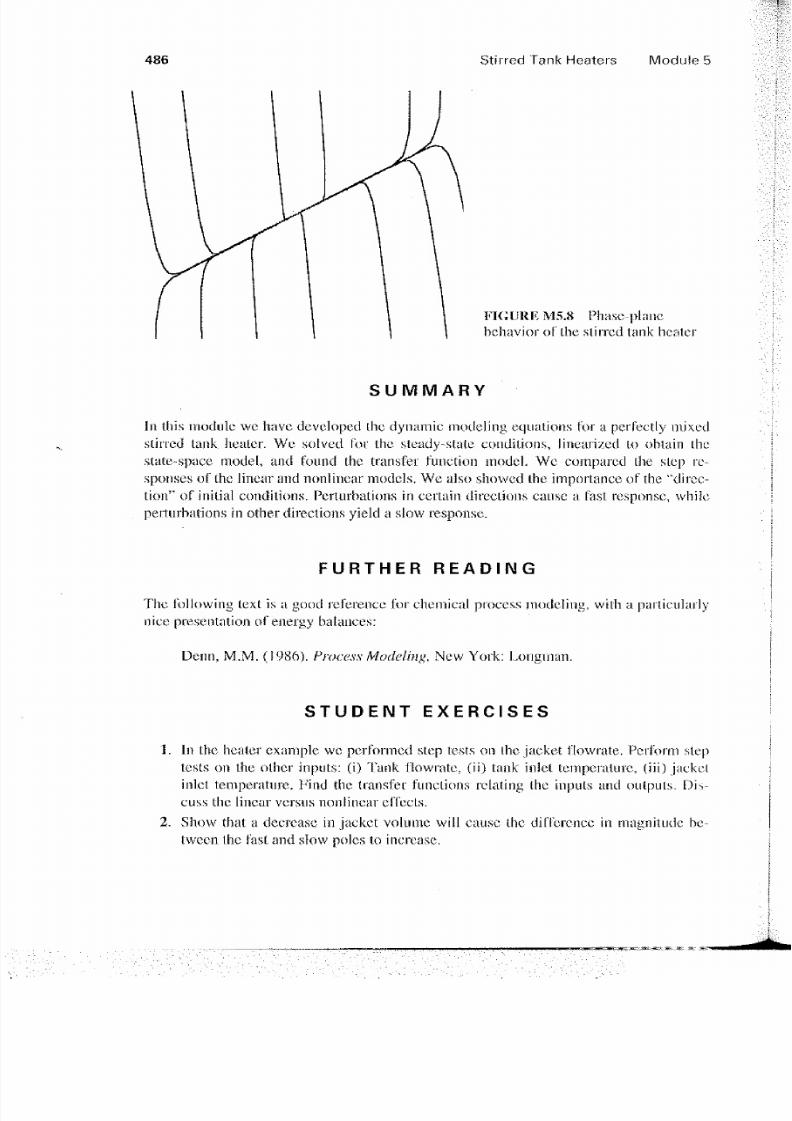
M 5 . 7 . 3 Ph a s e - P f a n e Be h a v io r

Thc phasc-plane heliavior is shown in Figure M5.S, whcre the Tank Temperature is plotted on thc x-axis and the Jacket Temperature is plotted on the v-axis. Noüce that iniliaíconditions in the [V ^i direction rcspond much more slowly íhan initíal conditions in thel " ™ ] direction.



486 S tirred T ank H eaters Moduie 5

FIGURE M5.8 Pha.se-planebehavior of the slirrcd tank healer

SUMMARY

Jn this module vve nave developed the dynamic modeling equations Cor a perfectly mixedstirred tank healer. We solved (br the sleady-stale condilions, linearized lo oblain thestate-space moclel, and found the transfer function inodel. We compared ihe slep re-sponses of the linear and noniinear models. We also showed ihe importance of the "diree-tion" of inilial condilions. PerUubations in cei'tain direclions cause a fast response, whilcperturbations in other direclions yield a slow response.

F U R T H E R R E A D I N G

The following lext is a good reference for chemical process modeling, wilh a particnlarlynice presentation of energy balances:

Denn, M.M. (1986). Process Modeling, New York: Longman.

S T U D E I M T E X E R C I S E S

1. In the healer cxample we perfonned step te.sts on the jacket flowrate. Pcri'orm sleptests on the olher inputs: (i) Tank flowrate, (ii) tank iniet ternperalure, (iii) jacketinlct temperature. Find the transfer funelions relating the inputs and outputs. Dis-cuss thc linear versus nonlinear effeets.

2. Show that a decrcase in jacket volunte will cause ihe differenee in magnitude be-tween the fast and slow poles to ulerease.



Appendix 487

Find the non linear steady-state relationships between jacket flowrate and the twolemperatmes (tank and jacket). Piol the inpul (jacket flowrate) versus the outputslor Che physical parameters given. Discuss how the gaín changes with coolantflowrate.

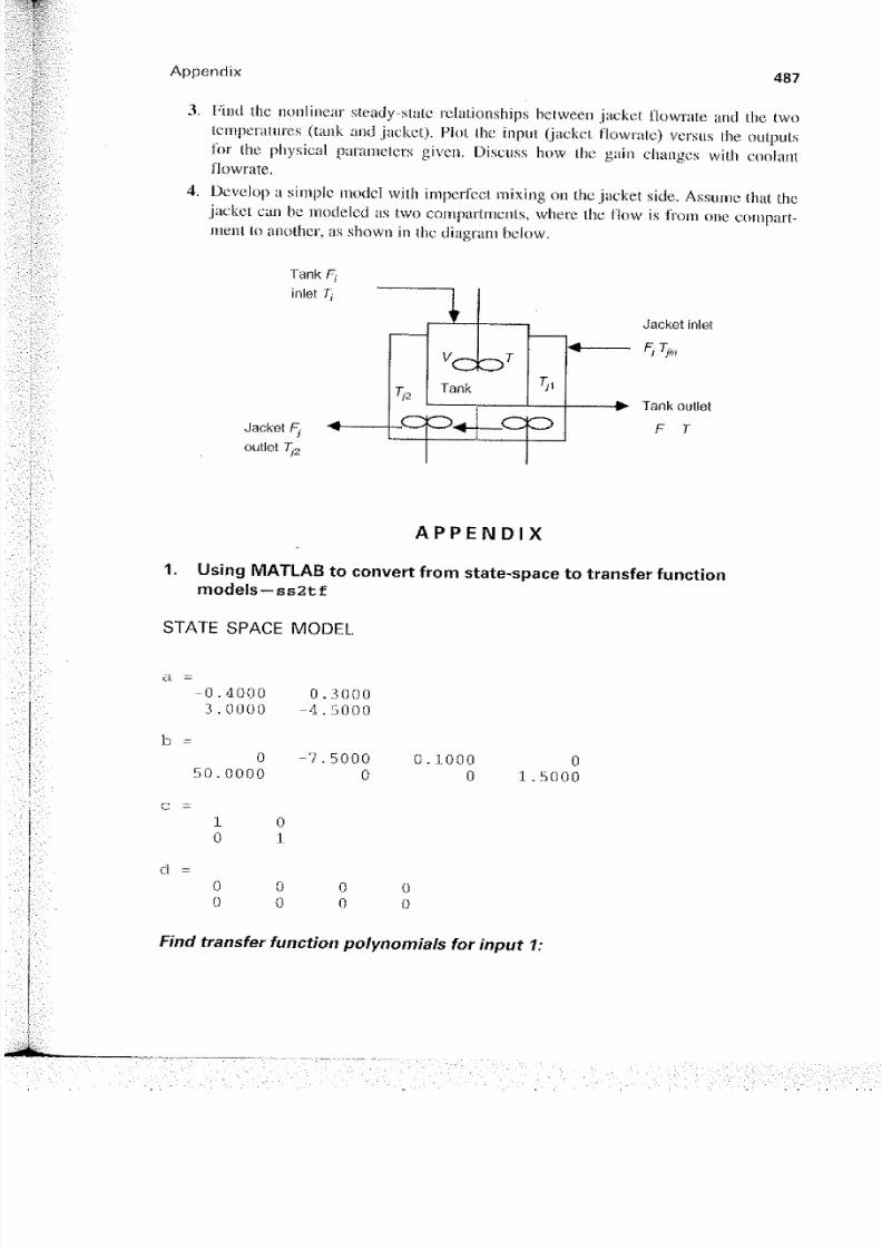
Develop a simple model with imperfeet mixing on the jacket síde. Assiime íhat thejacket can he mocleled as two compartmenis, where the flow i.s í'rom one compart-ment to another, as shown in the diagram below.

Tank F¡

inlet T¡

J acket F¡ "^outlet T¡ 2

TI2

^

K c d o r

Tank

o ^_

Tn

cz*™"»

J acket inlet

" * ' / >}M

F T

A P P E N D I X

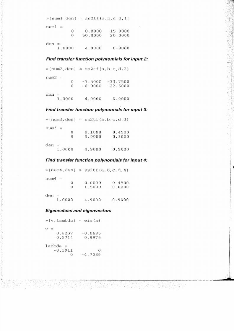
1 . Using MATLAB to convert f r om state-space to transfer functionmodels — s s 2tf

S T A T E S P A C E M O D E L

el =

- 0 . 4 0 0 03.0000

050 .0000

10

00

01

00

0- 4

- 7

300 0

5 00 0

50000

00

0.10000

00

01.5000

Find transfer function polynom ials for input 1:



» [ n um] , d e n] -- s s 2 t £ ( a, b, c , d, 1)

num =

O 0. 0000 15. 0000O 50 . 0000 20 . 0000

den -

1. 0000 4 . 9000 0 . 9000

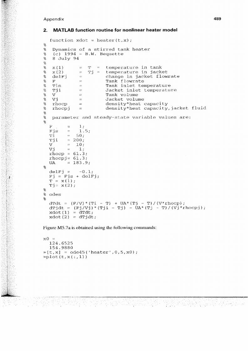
Fínd transfer function polynomials for input 2:

»[num2,den] ^ s s 2 t l ( a , b , e , d , 2 )

num2 =

O -7 .5000 -33 .7500O -0 .0000 -22 ,5000

den =

1.0000 4.9000 0.9000

Find transfer function polynomials for input 3:

»[num3,den] - s s 2 t £ ( a , b , c , d , 3 )

num3 =

O 0.1 000 0. 4500O 0.0 000 0. 3000

den -

1. 0000 4 . 9000 0 . 9000

Find transfer function polynomials for input 4:

»[num4,den] = s s 2 t f ( a , b , c , d , 4 )

num4 =

O 0. 0000 0. 4500O 1. 5000 0. 6000

den =

1.0000 4.9000 0 .9000

Eigenvalues and eigenvectors

» [ v , l a m b d a ] - e i g ( a )

v =

0. 82 07 0. 06950. 5714 0 . 9976

l ambda=-

- 0. 1911 O

O - 4 . 7 08 9



Appendi x 489

x ( l )x ( 2)de l F jFTi nTj iVVjr h o c pr h oc p j

=-===

:-

-

TTj

MA T L A B f unc t i on rout i ne f or noni i near heat er mode l

f unc t i on xdot = heat er ( t , x) ;

Dy na m cs of a s t i r r ed t ank hea te r( c) 1994 - B. W Bequet t e8 J ul y 94

t emper at ur e i n t ankt emperat ur a i n j acketcha nge i n j acket f l owr a t eTank f l owr a t eTank i nl et t emper a t ur eJ ac ket i nl et t emper a t u r eTank vol umeJ acket vol umedens i t y* heat c apac i t ydens i t y* heat c apac i t y, j ac ket f l ui d

%% par amet er and st eady- s t at é var i abl e val úes a r é :%

F = 1;F j s - 1. 5;Ti = 50;T j i = 200 ;V = 1 0 ;V 1;r hocp = 61. 3;r hocpj = 61. 3;UA = 183. 9;

%

del F j = - 0. 1;F j = F j s + del F j ;T = x (1) ;T j = x ( 2 ) ;

%% odes%

dT dt = ( P/ V) * ( T i - T ) + UA* ( T j - T ) / ( V* r ho c p) ;dT j dt ~ ( F j / Vj ) * ( T j i - Tj ) - UA* ( T j - T } / ( Vj * r h o c pj ) ;x dot ( l ) = dT dt ;x do t ( 2) = d Tj d t ;

Figure M5.7a is obtained using the following commands:

xO =124. 6525154. 9880

»[ t , x] = ode45( ' heat er ' , 0, 5, xO) ;»pl ot ( t , x( : , 1) )

modeling analysis and simulation(1)

Documents