Modeling, Analysis, and Control of a Class ofResource Allocation Systems Arising in

Concurrent Software

by

Hongwei Liao

A dissertation submitted in partial fulfillmentof the requirements for the degree of

Doctor of Philosophy(Electrical Engineering: Systems)in The University of Michigan

2012

Doctoral Committee:

Professor Stephane Lafortune, ChairProfessor Mingyan LiuProfessor Scott MahlkeProfessor Dawn TilburyProfessor Spyros Reveliotis, Georgia Institute of TechnologySenior Researcher Terence Kelly, HP LabsResearch Scientist Yin Wang, HP Labs

Liào Hóngwēi

c⃝ Hongwei Liao 2012

All Rights Reserved

ACKNOWLEDGEMENTS

I would like to express my deepest gratitude to my advisor, Professor Stephane

Lafortune, for his guidance. Through his advice and support, I have learned how to

grow as a professional researcher. He is not only my advisor on research, but also my

mentor on my career and many aspects beyond.

My special thanks also go to Professor Spyros Reveliotis, for his invaluable advice

and feedback on my work throughout this rigorous process. I would like to thank

Professor Scott Mahlke and Dr. Terence Kelly for their continuous encouragement,

thank Dr. Yin Wang for his long-term support, as well as give thanks to Professors

Dawn Tilbury and Mingyan Liu for accepting to sit on my dissertation committee.

I would like to sincerely thank Hyoun Kyu Cho for many suggestions on program

analysis; thank Jason Stanley for his continuous support on experimentation and

many inspiring discussions; thank Professors Mark Van Oyen and Ricardo Luders,

as well as my colleague, Hao Zhou, for their support on simulation analysis; and

thank Ahmed Nazeem for his comments on control synthesis. Also, I would like to

sincerely thank Dr. Sahika Genc, Dr. Weiling Wang, Dr. David VanderVeen, and

Guru Umasankar for their invaluable advice on my professional development.

I wish to acknowledge the financial support from NSF, HP Labs, EECS

Department Fellowship, and a Rackham Predoctoral Fellowship Award from the

Rackham Graduate School at the University of Michigan.

Finally, I would like to extend my deepest gratitude to my family for their constant

source of love, support, and encouragement.

ii

TABLE OF CONTENTS

ACKNOWLEDGEMENTS . . . . . . . . . . . . . . . . . . . . . . . . . . ii

LIST OF FIGURES . . . . . . . . . . . . . . . . . . . . . . . . . . . . . . . vi

LIST OF TABLES . . . . . . . . . . . . . . . . . . . . . . . . . . . . . . . . viii

ABSTRACT . . . . . . . . . . . . . . . . . . . . . . . . . . . . . . . . . . . ix

CHAPTER

I. Introduction . . . . . . . . . . . . . . . . . . . . . . . . . . . . . . 1

1.1 Challenges in the multicore era . . . . . . . . . . . . . . . . . 11.2 Overview of the Gadara project . . . . . . . . . . . . . . . . . 41.3 Discrete Event Systems Theory . . . . . . . . . . . . . . . . . 51.4 Main contributions . . . . . . . . . . . . . . . . . . . . . . . . 7

II. Modeling: The Class of Gadara Nets . . . . . . . . . . . . . . . 10

2.1 Introduction . . . . . . . . . . . . . . . . . . . . . . . . . . . 102.2 Modeling of multithreaded software . . . . . . . . . . . . . . 112.3 Petri net preliminaries . . . . . . . . . . . . . . . . . . . . . . 13

2.3.1 Standard definitions . . . . . . . . . . . . . . . . . . 142.3.2 Control synthesis for Petri nets . . . . . . . . . . . . 15

2.4 Gadara nets . . . . . . . . . . . . . . . . . . . . . . . . . . . 162.5 Controlled Gadara nets . . . . . . . . . . . . . . . . . . . . . 202.6 Uncontrollability in modeling . . . . . . . . . . . . . . . . . . 222.7 Discussion of related classes of Petri nets . . . . . . . . . . . 23

III. Analysis: Properties of Gadara Nets . . . . . . . . . . . . . . . 25

3.1 Introduction . . . . . . . . . . . . . . . . . . . . . . . . . . . 253.2 Petri net liveness and reversibility . . . . . . . . . . . . . . . 263.3 Resource-induced deadly marked siphons and modified markings 27

iii

3.4 The multithreaded program and its Gadara net model . . . . 293.5 Liveness of Gadara nets . . . . . . . . . . . . . . . . . . . . . 313.6 Reversibility of Gadara nets . . . . . . . . . . . . . . . . . . . 353.7 Linear separability and optimal control of Gadara nets . . . . 363.8 Verification of liveness using mathematical programming . . . 39

3.8.1 Key properties . . . . . . . . . . . . . . . . . . . . . 423.8.2 Verification of liveness of NG . . . . . . . . . . . . . 423.8.3 Verification of liveness of N c

G1 . . . . . . . . . . . . 453.8.4 Verification of liveness of N c

G . . . . . . . . . . . . . 473.8.5 Experimental results . . . . . . . . . . . . . . . . . 50

3.9 Case study: A deadlock bug in the Linux kernel . . . . . . . . 54

IV. Control I: Optimal Control of Gadara Nets – General Theory 58

4.1 Introduction . . . . . . . . . . . . . . . . . . . . . . . . . . . 584.2 Problem statement and motivation . . . . . . . . . . . . . . . 594.3 Overall strategy: Iterative control of Gadara nets . . . . . . . 624.4 Fundamentals of the UCCOR Algorithm . . . . . . . . . . . . 64

4.4.1 Definitions and partial-marking analysis . . . . . . . 644.4.2 Notion of covering . . . . . . . . . . . . . . . . . . . 674.4.3 Feasibility of maximally permissive control . . . . . 68

4.5 UCCOR Algorithm . . . . . . . . . . . . . . . . . . . . . . . 694.5.1 Unsafe Covering Construction Algorithm . . . . . . 714.5.2 Unsafe Covering Generalization . . . . . . . . . . . 724.5.3 Inter-Iteration Coverability Check . . . . . . . . . . 754.5.4 Monitor Place Synthesis Algorithm . . . . . . . . . 76

4.6 Properties . . . . . . . . . . . . . . . . . . . . . . . . . . . . . 824.6.1 Correctness and maximal permissiveness . . . . . . 824.6.2 Ordinariness of monitor places synthesized by UCCOR 86

4.7 Discussion of related approaches . . . . . . . . . . . . . . . . 88

V. Control II: Optimal Control of Gadara Nets – Customizationfor Ordinary Case . . . . . . . . . . . . . . . . . . . . . . . . . . . 90

5.1 Introduction . . . . . . . . . . . . . . . . . . . . . . . . . . . 905.2 Foundation for control synthesis . . . . . . . . . . . . . . . . 915.3 Overall strategy: Iterative control of ordinary Gadara nets . . 935.4 Optimal control algorithm based on RI empty siphons . . . . 95

5.4.1 UCCOR-O Algorithm: Overview . . . . . . . . . . . 955.4.2 Unsafe Covering Generation . . . . . . . . . . . . . 965.4.3 Unsafe Covering Generalization . . . . . . . . . . . 975.4.4 Monitor Place Synthesis Algorithm . . . . . . . . . 98

5.5 Properties . . . . . . . . . . . . . . . . . . . . . . . . . . . . . 1035.5.1 Properties of the UCCOR-O Algorithm . . . . . . . 1045.5.2 Properties of the ICOG-O Methodology . . . . . . . 106

iv

5.6 Experimental evaluation . . . . . . . . . . . . . . . . . . . . . 1085.6.1 Objective and setup of the experiments . . . . . . . 1095.6.2 Comparative analysis of ICOG-O and ICOG-O-ES . 1105.6.3 Scalability study of ICOG-O . . . . . . . . . . . . . 113

5.7 Discussion of applications . . . . . . . . . . . . . . . . . . . . 113

VI. Evaluation: Analysis of Program Models Using DiscreteEvent Simulation . . . . . . . . . . . . . . . . . . . . . . . . . . . 116

6.1 Introduction . . . . . . . . . . . . . . . . . . . . . . . . . . . 1166.2 Stochastic timed Gadara net model . . . . . . . . . . . . . . . 1176.3 The discrete event simulation model . . . . . . . . . . . . . . 1186.4 Performance metrics . . . . . . . . . . . . . . . . . . . . . . . 120

6.4.1 Measure of safety . . . . . . . . . . . . . . . . . . . 1206.4.2 Measure of efficiency . . . . . . . . . . . . . . . . . 1216.4.3 Measure of activity level . . . . . . . . . . . . . . . 121

6.5 Case studies . . . . . . . . . . . . . . . . . . . . . . . . . . . 1226.5.1 Case study 1: A deadlock scenario in OpenLDAP . 1226.5.2 Case study 2: Two threads sharing three resources . 125

6.6 Discussion of related work and applications . . . . . . . . . . 129

VII. Conclusion . . . . . . . . . . . . . . . . . . . . . . . . . . . . . . . 133

7.1 Summary of main contributions . . . . . . . . . . . . . . . . . 1337.2 Future work . . . . . . . . . . . . . . . . . . . . . . . . . . . 135

BIBLIOGRAPHY . . . . . . . . . . . . . . . . . . . . . . . . . . . . . . . . 137

v

LIST OF FIGURES

Figure

1.1 The Gadara project architecture . . . . . . . . . . . . . . . . . . . . 4

2.1 A deadlock example in BIND: (a) Simplified code; (b) Gadara netmodel . . . . . . . . . . . . . . . . . . . . . . . . . . . . . . . . . . 13

3.1 Example: S = {pc1 , pc2 , p12, p13, p22, p23} is a nonempty RIDM siphonat the marking shown in the figure . . . . . . . . . . . . . . . . . . 28

3.2 A deadlock example in BIND: Controlled Gadara net model . . . . 40

3.3 Sample statistics: (a) MIP-N cG1 vs. MIP-ES; (b) MIP-N c

G vs. MIP-RS 51

3.4 Normalized Cumulative Frequency (NCF): (a) MIP-N cG1 vs. MIP-ES;

(b) MIP-N cG vs. MIP-RS . . . . . . . . . . . . . . . . . . . . . . . . 52

3.5 A deadlock example in the Linux kernel: Simplified code . . . . . . 56

3.6 A deadlock example in the Linux kernel: Gadara net model . . . . . 57

4.1 A running example of control synthesis using ICOG . . . . . . . . . 61

4.2 Iterative control of Gadara nets (ICOG) . . . . . . . . . . . . . . . 63

4.3 UCCOR Algorithm . . . . . . . . . . . . . . . . . . . . . . . . . . . 70

4.4 The constraint transformation technique used in Stage 2 of theMonitor Place Synthesis Algorithm . . . . . . . . . . . . . . . . . . 78

4.5 Gadara net model of a deadlock example in the OpenLDAP software 80

4.6 A simple example of UCCOR . . . . . . . . . . . . . . . . . . . . . 81

vi

4.7 Illustration of the rearranged order of rows in a marking, covering,and incidence matrix . . . . . . . . . . . . . . . . . . . . . . . . . . 87

5.1 Iterative control of Gadara nets: Ordinary case (ICOG-O) . . . . . 93

5.2 Flowchart of the UCCOR-O Algorithm . . . . . . . . . . . . . . . . 96

5.3 A deadlock example in the Linux kernel: Controlled Gadara net model100

5.4 The constraint transformation technique used in Stage 2 of theMonitor Place Synthesis Algorithm . . . . . . . . . . . . . . . . . . 101

5.5 Cases considered in the proof: (a) Case 1; (b) Case 2; (c) Case 3;(d) Case 4 . . . . . . . . . . . . . . . . . . . . . . . . . . . . . . . . 105

5.6 (a) TTC of ICOG-O and ICOG-O-ES: Normalized cumulative fre-quency; (b) TTC of ICOG-O and ICOG-O-ES: Estimated probabilitydensity function; (c) Difference of the number of iterations of ICOG-O-ES and ICOG-O . . . . . . . . . . . . . . . . . . . . . . . . . . . 111

6.1 Enhanced event list . . . . . . . . . . . . . . . . . . . . . . . . . . . 119

6.2 Pd of uncontrolled program model under various values of (π4, π6) . 124

6.3 MTTF under various values of (π4, π6): (a) Before control; (b) Aftercontrol; (c) Overhead . . . . . . . . . . . . . . . . . . . . . . . . . . 124

6.4 β under various values of (π4, π6): (a) Before control; (b) Aftercontrol; (c) Overhead . . . . . . . . . . . . . . . . . . . . . . . . . . 125

6.5 A Gadara net model of two threads sharing three resources . . . . . 127

6.6 Sensitivity analysis results for Strategy 2: (a) Pd; (b) MTTF; (c) β . 128

6.7 Deadlock probability reduction rate of Strategy 2 . . . . . . . . . . 129

6.8 Control Strategy Maps: (a) Tradeoff between Pd and MTTF;(b) Tradeoff between Pd and β . . . . . . . . . . . . . . . . . . . . . 130

vii

LIST OF TABLES

Table

3.1 Experimental results of comparative analysis on liveness verificationalgorithms . . . . . . . . . . . . . . . . . . . . . . . . . . . . . . . . 54

5.1 Experimental results of comparative analysis between ICOG-O andICOG-O-ES . . . . . . . . . . . . . . . . . . . . . . . . . . . . . . . 114

5.2 Experimental results of scalability study of ICOG-O . . . . . . . . . 115

6.1 Definition of control strategies . . . . . . . . . . . . . . . . . . . . . 128

viii

ABSTRACT

Modeling, Analysis, and Control of a Class of Resource Allocation SystemsArising in Concurrent Software

by

Hongwei Liao

Chair: Stephane Lafortune

In the past decade, computer hardware has undergone a true revolution, moving from

uniprocessor architectures to multiprocessor architectures, or multicore. In order to

exploit the full potential of multicore hardware, there is an unprecedented interest in

parallelizing the applications that were previously conducted in sequential order. This

trend forces parallel programming upon the average programmer. However, reasoning

about concurrency is challenging for human programmers. Significant effort has been

spent to eliminate several types of concurrency bugs.

In this dissertation, we study the modeling, analysis, control, and evaluation of a

class of resource allocation systems arising in concurrent software using Petri nets, a

commonly used modeling formalism in Discrete Event Systems. We formally define

a new class of Petri nets, called Gadara nets, to systematically model multithreaded

programs with lock allocation and release operations, a widely used programming

paradigm for concurrent software with shared data. We focus on an important class

of concurrency bugs, known as circular-mutex-wait deadlocks, or simply deadlocks.

Deadlock-freeness of a program corresponds to liveness of its Gadara net model. We

ix

establish necessary and sufficient conditions for liveness and reversibility properties of

Gadara nets, which lay the foundations for their control synthesis. We propose a new

liveness-enforcing control synthesis methodology for general Gadara nets that need

not be ordinary. The method is based on structural analysis and converges in finite

iterations. It is shown to be correct and maximally permissive with respect to the

goal of liveness enforcement. We further customize this control synthesis methodology

for ordinary Gadara nets and establish a set of important properties. Performance

evaluations are conducted for comparing the original and controlled program models,

using Discrete Event Simulation. Our results are applied to the analysis of large-scale

multithreaded program models, showing that our approach is scalable to real-world

software. Finally, we discuss potential directions for future work.

x

CHAPTER I

Introduction

1.1 Challenges in the multicore era

A fundamental revolution has taken place in the computer industry in the past

decade. The mainstream computer CPUs used to have only a single processor core

capable of executing a single task at a time. CPU speeds doubled roughly every 18

months according to Moore’s law. Processor core speed cannot increase indefinitely,

however, because faster cores generate excessive heat. Successive CPU generations

therefore now provide more processor cores rather than a faster single core and can

execute several tasks at once.

The revolution of computer hardware from uniprocessor architectures to multi-

processor architectures also leads to some challenges. One problem is that only

parallel software can exploit the full performance potential of multicore architectures,

and parallel software is far harder to write than conventional serial software.

Choreographing a productive and harmonious interplay among concurrent tasks is

very difficult because reasoning about concurrency is very challenging for human

programmers. Multicore architectures are making parallel programming unavoidable

but concurrency bugs are making it costly and error-prone. Significant effort has been

spent to eliminate several types of concurrency bugs; see, e.g., [84, 77, 78, 79, 72, 82].

In this dissertation, we are interested in shared-memory multithreaded software,

1

a very common computing paradigm in which concurrent tasks share access to a

pool of computer memory. Mutual exclusion locks (or “mutexes”) prevent tasks

from accessing the same memory concurrently, thus allowing tasks to update shared

memory in an orderly way, because a given lock may be held by at most one task

at any moment. However, it is easy for situations to arise in which, e.g., task 1

has acquired lock A and needs lock B, while task 2 holds B but requires A; these

tasks are deadlocked and neither can perform useful work. Such deadlocks are called

circular-mutex-wait (CMW) deadlocks in the literature, where a set of threads is

waiting indefinitely and no thread can proceed. In this dissertation, we focus on

CMW deadlocks, an important class of failures arising in concurrent software.

Development of highly reliable and robust software is a very active research area in

the software and operating systems communities. The “Rx” system proposed in [84]

responds to failures by rolling back execution state to a previous checkpoint and re-

executing after heuristically perturbing the execution environment in an attempt to

prevent recurrence of the failure. For example, replacing default memory allocation

mechanisms with safer and more conservative alternatives may prevent recurrence of

failures attributed to memory corruption. Rx repeats the rollback/perturbation/re-

execution cycle until the software successfully executes beyond the failure or a

timeout occurs; the latter indicates that Rx’s heuristic approach cannot address the

failure. “Bouncer” [13] generates filters to prevent potential exploits of software

vulnerabilities, based on heuristics and learning from practice. “ASSURE” [94]

uses a self-healing method, called rescue points, to recover software from faults in

server applications. In case of a fault, the system restores to the closest rescue

point and attempts to recover by employing the existing error-handling facilities.

“Exterminator” [78, 79] detects, isolates, and corrects certain classes of memory

errors. After pinpointing the cause of an error, Exterminator automatically generates

patches to correct the software that experienced it. These patches may be shared

2

among users of the same software, thus enabling automated collaborative bug

remediation. The works above address various types of failures and reliability issues

in software and operating systems.

When it comes to the specific issue of program deadlock, many approaches

have been proposed for deadlock analysis and resolution. Variants of the Banker’s

Algorithm [15, 16] provide a principled approach to dynamic deadlock avoidance

for concurrent software. The algorithm, however, requires a central controller that

can potentially impose a global serial bottleneck on the software it governs. Deadlock

“Healing” [77] addresses potential deadlocks by adding “gate locks” that prevent out-

of-order lock acquisitions from causing deadlocks. At runtime, actual deadlocks are

detected and remedied by adding further gate locks, gradually eliminating deadlocks

from programs. Healing is more practical than the Banker’s Algorithm because its

runtime checks are efficient and because it does not introduce a global serialization

point into the software that it controls. Another deadlock avoidance approach is

“Dimmunix” [44, 45], which equips the software system with an “immune system”.

The deadlock immunity can resist future occurrences of similar deadlocks, and it is

obtained by learning from the control flows that led to deadlocks. Reference [111]

employs Just-in-time compilation techniques and exploits deadlock patterns at

runtime, so that deadlocks of the same patterns can be avoided in the future.

A randomized dynamic technique is presented in [43] for deadlock detection in

multithreaded programs. This technique uses a random scheduler to create real

deadlocks with high probability in a two-stage process, and it does not report any false

positives. References [24, 25] propose a type and effect system to dynamically avoid

deadlocks, by using the information of lock operations that is computed statically. A

key feature of this system is that it does not assume block-structured locking or a

strict order of lock allocation.

In spite of the above approaches toward software reliability and robustness, there

3

is an emerging need for systematic methodologies that will enable programmers to

characterize, analyze, and resolve software failures, such as deadlocks.

1.2 Overview of the Gadara project

The broad context for the research work reported in this dissertation is the Gadara

project [98, 48, 108]. The objective of the Gadara project is to develop a software tool

that takes as input a deadlock-prone multithreaded C program and outputs a modified

version of the program that is guaranteed to run deadlock-free without affecting any

of the functionalities of the program. The system architecture of the Gadara project

is shown in Figure 1.1, which includes four stages [104].

C program

source code

control

flow graph

Petri net control

logic

1. compilation

2. translation

3. control

logic

synthesis

4.

inst

rum

enta

tio

n

instrumented executable

pro

gra

m

compile

observe

control

observe

control

observe

control

con

tro

l lo

gic

offline online

Figure 1.1: The Gadara project architecture

1. The C program source code is converted into a Control Flow Graph (CFG)

by compiler techniques. A CFG is a high-level graphical representation of all

code execution paths that might be traversed by the program. The CFG is

augmented with additional information about lock variables and lock functions.

The enhanced CFG is a directed graph.

2. The enhanced CFG is translated into a Petri net model of the program, formally

4

defined as a Gadara net, based on which potential deadlocks in the program

can be mapped to structural features in the net.

3. Optimal control logic is synthesized for the Gadara net. The output of this step

is a controlled Gadara net, augmented with monitor (a.k.a. control) places,

which corresponds to a CMW-deadlock-free program.

4. The synthesized control logic captured by the monitor places is incorporated

into the program by instrumenting the original code.

The four steps described above are all conducted off-line. During program

execution, the only on-line overhead is due to the additional lines of code pertaining

to checking and updating the contents of the monitor places. In this dissertation,

we focus on Steps 2 and 3, and we systematically model, analyze, and control

multithreaded software for the purpose of deadlock avoidance. The details on Steps

1 and 4 are reported in [103, 104, 105].

1.3 Discrete Event Systems Theory

In view of the event-driven nature of program dynamics and the logical control

specification of deadlock avoidance, we adopt a model-based approach by employing

the techniques from Discrete Event Systems (DES) Theory [8]. Discrete event systems

are a class of dynamic systems that have discrete state spaces and event-driven

dynamics. While classical control theory, which focuses on time-driven systems,

has been successfully applied to computer systems [34], the application of DES

to computer systems is more recent; see, e.g., [101, 83, 65, 17, 3, 22, 40, 14, 49].

Concurrent software is a typical example of a DES.

Finite state automata and Petri nets are the two most popular modeling

formalisms for DES. We chose Petri nets as our modeling formalism, because there

are at least three advantages of using Petri nets in this application context: (i) Petri

5

nets provide a compact, graphical representation of a concurrent program’s inherent

dynamics, without explicitly enumerating its state space; (ii) the Petri net models

enable formal analysis and verification of important properties of their associated

programs via efficient structural analysis; (iii) the models also make possible the

synthesis of provably correct and optimal control logic that can be instrumented in

the original programs for deadlock avoidance at run-time.

Deadlock analysis based on Petri nets has been widely studied for flexible

manufacturing systems and other technological applications involving a resource

allocation function [56, 88]. Various special classes of Petri nets have been proposed

to analyze manufacturing systems [56]. Recently, there has also been a growing

interest in the application of DES to software systems and embedded systems. A

review of the application of Petri nets to computer programming is presented in [39].

Modeling thread creation/termination and mutex lock/unlock operations is in fact

a classical application of Petri nets [70]; in particular, Petri nets were used in the

static analysis and deadlock analysis of Ada programs [92, 71, 93]. In the case of the

popular Pthread library for C/C++ programs, Petri nets have also been employed to

model multithreaded synchronization primitives [47].

The results presented in this dissertation allow us to specialize the existing

theory of Petri net-based deadlock analysis and avoidance for sequential resource

allocation systems. We can then apply this theory to lock allocations in shared-

memory multithreaded software. At the same time, the results take advantage of

the additional structure that is present in the considered resource allocation function

in order to substantially strengthen and extend the existing theory. A more detailed

discussion of the main contributions of this dissertation is provided in the next section.

Furthermore, additional reviews of related work will be presented throughout the

dissertation.

6

1.4 Main contributions

The main contributions and organization of this dissertation are summarized as

follows.

• Chapter II: Modeling ([64, 107]). We formally define a new class of Petri

nets, called Gadara nets, to systematically model multithreaded programs with

lock allocation and release operations. The class of Gadara nets explicitly

models the locking behavior of multithreaded programs and enables the

efficient characterization of the CMW deadlocks of programs through structural

analysis. Gadara nets also capture some special features of programs, e.g., in

general, these nets are cyclic due to the modeling of loops, and they contain

uncontrollable transitions due to the modeling of branch selections.

• Chapter III: Analysis ([64, 61, 107]). We investigate a set of important

properties of Gadara nets, such as liveness, reversibility, and linear separability.

Based on these properties, deadlock-freeness – a behavioral property – of the

program corresponds to liveness of its Gadara net model, which can in turn

be analyzed via the structural properties of the net in terms of siphons. For

the verification of the liveness property, we propose a set of mathematical

programming formulations, which are customized for Gadara nets.

• Chapter IV: Control – General theory ([60, 59]) and Chapter V: Control –

Customization ([62, 61]). We propose a new liveness-enforcing control synthesis

methodology for general Gadara nets that need not be ordinary. The method

is based on structural analysis and converges in a finite number of iterations.

It is shown to be correct and maximally permissive with respect to the goal of

liveness enforcement. We further customize this control synthesis methodology

for the particular application of concurrent software, where we always have an

ordinary Gadara net as the initial condition. We show that the customized

7

method will never synthesize redundant control logic throughout the control

iterations.

• Chapter VI: Evaluation ([63]). We extend the class of untimed Gadara nets

to the class of stochastic timed Gadara nets and propose a customized discrete

event simulation methodology for the extended class. We conduct simulation

analysis on the Gadara net models of programs before and after control, where

the performance metrics related to safety, efficiency, and activity level are

studied via output data analysis. We further conduct sensitivity analysis on

these Gadara net models and investigate the effect of key parameters on the

programs. We also discuss the implication of the simulation results for deadlock-

avoidance control.

• Chapter VII: Conclusion. We summarize the main contributions of this

dissertation and discuss the potential directions for future work.

The property of the proposed control synthesis methodology discussed above,

namely the maximally-permissive liveness-enforcing (MPLE) property, is also called

“optimal” in this dissertation. In the context of program deadlock avoidance,

optimality refers to the elimination of deadlocks in the program with minimally

restrictive control logic.

As a technical note, the two terminologies, “deadlock” and “deadlock avoidance”,

have different meanings in the software engineering and control engineering commu-

nities. We make the following remarks for the sake of clarity.

Remark I.1. The notion of “deadlock” we discussed above refers to the CMW-

deadlock of a program; in the Petri net literature, “deadlock” usually refers to the

case where all the transitions in the net are disabled. To avoid any confusion, in the

rest of this dissertation, we refer to these two types of deadlocks as CMW-deadlock

(Definition II.1) and total-deadlock (Definition III.4), respectively. When the context

8

provides no confusion, we sometimes refer to “CMW-deadlock” as “deadlock” for

the sake of simplicity. Moreover, as we will show in Chapter III, in order to avoid

the CMW-deadlocks of a program, we require liveness of its corresponding Petri net

model. Therefore, the key Petri net property under study in this dissertation is

liveness, rather than total-deadlock-freeness. �

Remark I.2. Our strategy corresponds to what is termed “deadlock avoidance” in

computer systems [96]; in the Petri net literature, such strategies are usually classified

as “deadlock prevention” [56]. �

9

CHAPTER II

Modeling: The Class of Gadara Nets

2.1 Introduction

As discussed in Chapter I, various special classes of Petri nets have been proposed

to analyze resource allocations of manufacturing systems [56]. We discovered that the

existing special classes of Petri nets in the literature do not exactly match the specific

features of Petri nets that arise when modeling the locking behavior of multithreaded

programs. Therefore, we propose a new class of Petri nets, called Gadara nets,

that systematically models multithreaded programs with lock allocation and release

operations. With the class of Gadara nets formally defined, we can efficiently analyze

program deadlocks via formal models and synthesize deadlock avoidance control

policies, which can in turn be instrumented in the underlying programs.

This chapter is organized as follows. We present some background about the

modeling of multithreaded software in Section 2.2, and we introduce the Petri

net preliminaries in Section 2.3. The class of Gadara nets is formally defined in

Section 2.4, and the class of controlled Gadara nets is further defined in Section 2.5.

We discuss the issue of uncontrollability in modeling in Section 2.6, and we review

the related classes of Petri nets in Section 2.7. Some of the results in this chapter

also appear in [64, 107].

10

2.2 Modeling of multithreaded software

We first introduce the definition of a CMW-deadlock.

Definition II.1. A program is said to be in a CMW-deadlock if there exists a circular

chain of two or more threads in the program, where each thread in the chain waits

for a mutex that is held by the next thread in the chain, and none of the threads can

proceed.

Determining if a program is deadlock-free, for any type of deadlock, is undecidable,

as it is a special instance of the halting problem for Turing machines [35]. We overcome

this obstacle by focusing on CMW-deadlocks and by making modeling assumptions.

A key challenge is scalability. Real-world large-scale software contains thousands

of functions and millions of lines of code. Inlining the whole program, which is

required for CMW-deadlock analysis, is not an option. We first prune functions and

code regions that are irrelevant to deadlock analysis. We apply lock graph analysis

[18, 7] to isolate the code regions that are subject to CMW-deadlock, and inline

only the tail of the whole call stack that fully contains the CMW-deadlock. After

pruning and lock graph analysis, we obtain a manageable model that is tractable for

the analysis of mutex interactions and CMW deadlocks. In addition to scalability,

language features also pose difficulties, e.g., recursion, function pointers, and dynamic

locks. When in doubt about what particular lock a given call refers to, we model the

lock in a conservative way [104]. Finally, there are Operating System, C language,

and Pthread library specific features that we do not currently model, e.g., UNIX

Inter-Process Communication calls that can result in other types of deadlocks, and

setjump, longjump functions in C. Using all of the above techniques and under

the above restrictions, we are able to capture all CMW-deadlocks in multithreaded

programs using Petri nets.

As discussed above, a wide range of sub-classes of Petri nets have been proposed

11

in the literature, most of them motivated by applications in flexible manufacturing

systems. Similarly, the class of Gadara nets formally defined in this chapter is

motivated by the application domain of concurrent software, with a focus on the

analysis of CMW-deadlocks. A Petri net model is obtained in Step 2 of the Gadara

architecture in Figure 1.1 by translating the enhanced CFG of the program. We create

a place to represent each node (i.e., basic block) in the enhanced CFG. Moreover, a

directed arc connecting two nodes in the enhanced CFG is represented by a transition

and associated arcs in the Petri net. For example, if there is an arc−→AB in the enhanced

CFG that connects node A to node B, then in the corresponding Petri net model, the

two nodes A and B are represented by two places pA and pB, respectively; further,

−→AB is represented by three components in the Petri net: a transition t, an arc from

pA to t, and another arc from t to pB. Lock variables are also modeled by places,

whose connectivity to the transitions is determined by the actions of lock acquisitions

or releases of the program. If a transition represents a lock acquisition call, we add

an arc from the place modeling the lock to the transition; if a transition represents a

lock release call, we add an arc from the transition to the place modeling the lock. A

token in a place that represents a basic block models a thread executing in this basic

block; a token in a place that represents a lock models the availability of this lock.

The final Petri net model is called a Gadara net.

To facilitate our discussion, we will use a deadlock bug in the BIND software as

a running example, which is shown in Figure 2.1. The acronym BIND stands for

“Berkeley Internet Name Daemon,” which is a popular Domain Name System (DNS)

on the Internet. Figure 2.1(a) shows the lines of code that are related to the deadlock

under consideration; the corresponding Gadara net model is shown in Figure 2.1(b).

The deadlock occurs if there is one token in p1, which represents one thread holding

lock A while waiting for lock B, and there is one token in p4, which represents another

thread holding lock B while waiting for lock A. This deadlock bug occurred in the

12

(a) (b)

Figure 2.1: A deadlock example in BIND: (a) Simplified code; (b) Gadara net model

final release version 9.2.2, and was fixed in the release candidate version 9.2.3rc1. As

the bug database of BIND is not open to the public, we confirmed the bug by the

change log of 9.2.3rc1, as well as using source code comparison. The bug resided in the

rbtdb.c file, which is a red black tree data structure that stores domain names and

IP addresses. For the sake of discussion, the Gadara net model has been simplified;

in particular, we model the Reader/Writer lock in this example as a mutex.

2.3 Petri net preliminaries

Before introducing the formal definition of Gadara nets, we first briefly review

some Petri net preliminaries; see [70, 8] for a detailed discussion.

13

2.3.1 Standard definitions

Definition II.2. A Petri net dynamic system N = (P, T,A,W,M0) is a bipartite

graph (P, T,A,W ) with an initial number of tokens. Specifically, P = {p1, p2, ..., pn}

is the set of places, T = {t1, t2, ..., tm} is the set of transitions, A ⊆ (P ×T )∪ (T ×P )

is the set of arcs, W : A → {1, 2, ...} is the arc weight function, and for each p ∈ P ,

M0(p) is the initial number of tokens in p.

The marking (a.k.a. state) of a Petri net N is a column vector M of n entries

corresponding to the n places. As defined above, M0 is the initial marking. We use

M(p) to denote the (partial) marking on a place p, which is a scalar; we use M(Q) to

denote the (partial) marking on a set of places Q, which is a |Q| × 1 column vector.

The notation •p denotes the set of input transitions of place p: •p = {t|(t, p) ∈ A}.

Similarly, p• denotes the set of output transitions of p. The sets of input and output

places of transition t are similarly defined by •t and t•. This notation is extended to

sets of places or transitions in a natural way.

A transition t is enabled or fireable at M , if ∀p ∈ •t, M(p) ≥ W (p, t). When an

enabled transition t fires, for each p ∈ •t, it removes W (p, t) tokens from p; and for

each q ∈ t•, it adds W (t, q) tokens to q. The reachable state space R(N ,M0) of N is

the set of all markings reachable by transition firing sequences starting from M0.

A pair (p, t) is called a self-loop if p is both an input and output place of t.

We consider only self-loop-free Petri nets in this dissertation. A Petri net is called

ordinary if all the arcs in the net have unit arc weights, i.e., W (a) = 1, ∀a ∈ A;

otherwise, it is called non-ordinary. Without any confusion, we can drop W in the

definition of any Petri net N that is ordinary.

Definition II.3. The incidence matrix D of a Petri net is an integer matrix D ∈

Zn×m, where Dij = W (tj, pi)−W (pi, tj) represents the net change in the number of

tokens in place pi when transition tj fires.

14

Definition II.4. A state machine is an ordinary Petri net such that each transition t

has exactly one input place and exactly one output place, i.e., ∀t ∈ T, |•t| = |t•| = 1.

Definition II.5. Let D be the incidence matrix of a Petri net N . Any non-zero

integer vector y such that DTy = 0 is called a P-invariant of N . Further, P-invariant

y is called a P-semiflow if all the elements of y are non-negative.

By definition, P-semiflow is a special case of P-invariant. A straightforward

property of P-invariants is given by the following well-known result [70]: If a vector

y is a P-invariant of Petri net N = (P, T,A,M0), then we have MTy = MT0 y for any

reachable marking M ∈ R(N ,M0). The support of P-semiflow y, denoted as ∥y∥, is

defined to be the set of places that correspond to nonzero entries in y. A support

∥y∥ is said to be minimal if there does not exist another nonempty support ∥y′∥, for

some other P-semiflow y′, such that ∥y′∥⊂∥y∥. A P-semiflow y is said to be minimal

if there does not exist another P-semiflow y′ such that y′(p) ≤ y(p), ∀p. For a given

minimal support of a P-semiflow, there exists a unique minimal P-semiflow, which

we call the minimal-support P-semiflow [70].

2.3.2 Control synthesis for Petri nets

Supervision Based on Place Invariants (SBPI) [28, 27, 110, 68, 38] provides an

efficient algebraic technique for control logic synthesis by introducing a monitor place,

which essentially enforces a P-invariant so as to achieve a given linear inequality

constraint of the following form

lTM ≤ b (2.1)

where M is the marking vector of the net under control, l is a weight (column) vector,

and b is a scalar. All entries of l and b are integers. The main result of SBPI is as

follows.

15

Theorem II.1. [38] Consider a Petri net N , with incidence matrix D and initial

marking M0. If b − lTM0 ≥ 0, then a monitor place, pc, with incidence matrix

Dpc = −lTD, and initial marking M0(pc) = b−lTM0, enforces the constraint lTM ≤ b

upon the net marking. This supervision is maximally permissive.

The property of maximal permissiveness stated in the above theorem implies that

a transition in the net is disabled by the monitor place only if its firing leads to a

marking where the linear constraint in (2.1) is violated.

2.4 Gadara nets

Gadara nets, first introduced in [107, 64], are a special class of Petri nets that

models multithreaded C programs with lock allocation and release operations, for the

purpose of CMW-deadlock avoidance. In this section, we formally define the class of

Gadara nets.

As discussed in Section 2.2, Gadara nets are translated from the enhanced CFG

of multithreaded programs. They provide a formal foundation to model the locking

behavior (case of mutexes) of the program. Gadara nets share features with classes

of Petri nets that arise in the modeling of manufacturing systems [88, 56]. More

specifically, they consist of a set of process subnets that correspond to thread entry

points in the program, and resource places that model the locks through which threads

interact.

Definition II.6. Let IN = {1, 2, ...,m} be a finite set of process subnet indices. A

Gadara net is an ordinary, self-loop-free Petri net NG = (P, T,A,M0) where

1. P = P0 ∪ PS ∪ PR is a partition such that: a) PS =∪

i∈IN PSi, PSi

= ∅, and

PSi∩ PSj

= ∅, for all i = j; b) P0 =∪

i∈IN P0i , where P0i = {p0i}; and

c) PR = {r1, r2, ..., rk}, k > 0.

2. T =∪

i∈IN Ti, Ti = ∅, Ti ∩ Tj = ∅, for all i = j.

16

3. For all i ∈ IN , the subnet Ni generated by PSi∪{p0i}∪Ti is a strongly connected

state machine. There are no direct connections between the elements of PSi∪

{p0i} and Tj for any pair (i, j) with i = j.

4. ∀p ∈ PS, if |p • | > 1, then ∀t ∈ p•, •t ∩ PR = ∅.

5. For each r ∈ PR, there exists a unique minimal-support P-semiflow, Yr, such

that {r} = ∥Yr∥ ∩PR, (∀p ∈ ∥Yr∥)(Yr(p) = 1), P0 ∩ ∥Yr∥= ∅, and PS ∩ ∥Yr∥= ∅.

6. ∀r ∈ PR,M0(r) = 1, ∀p ∈ PS,M0(p) = 0, and ∀p0 ∈ P0,M0(p0) ≥ 1.

7. PS =∪

r∈PR(∥Yr∥ \{r}).

A Gadara net NG is defined to be an ordinary Petri net, because it models

programs with mutex locks. Condition 1 classifies the set of places in NG into

three types: (i) The idle place p0i ∈ P0 is an artificial place added to facilitate the

discussion of liveness and other properties. The tokens in an idle place represent the

threads that “wait” for future execution. (ii) PS is the set of operation places. Each

operation place models a basic block of the program. A token in an operation place

represents one instance of thread that is executing in the current basic block. (iii) PR

is the set of resource places that model mutex locks. A token in a resource place

represents the availability of the mutex lock. For example, in the Gadara net shown

in Figure 2.1(b), place p0 is an idle place, places rA and rB are resource places, and

the other places in the net are operation places.

Condition 2 defines the set of transitions in NG. Each subnet of NG has its

own set of transitions, which is not shared by any other subnet. A transition in NG

models the action of lock acquisition or release by the program; a transition can also

model branches in the program, such as if/else. NG consists of a set of subnets

Ni that define work processes, called process subnets in the literature. Based on

process subnet Ni, if we further consider the resource places (and monitor places

17

to be introduced in the next section) associated with it, then the resulting net is

called a resource-augmented process subnet, denoted as N augi . Unlike most prior work

in manufacturing applications, our process subnets need not be acyclic, due to the

modeling of loops in programs. We observe from Figure 2.1(b) that the concurrent

execution of multiple threads can even be modeled by one process subnet with multiple

tokens in different operation places.

In Condition 3, the restriction of the process subnets Ni to the class of state

machines implies that there is no “forking” or “joining” in these subnets. The state

machine structure of a process subnet is a natural result of the translation of the

enhanced CFG as described in Section 2.2. On the other hand, the strong connectivity

of the subnets Ni, which is also stipulated by Condition 3, ensures that in the

dynamics of these subnets, a token starting from the idle place will always be able to

come back to the idle place after processing. In more natural terms, this requirement

for strong connectivity implies that the only reason that might prevent the completion

of the considered processes is their contest for the locks that govern their access to

their critical sections and not any other potential errors in the underlying program

logic. Further, the process subnets are interconnected only by resource places, i.e.,

any operation place or idle place in Ni does not connect to any transition in Nj, for

i = j.

Condition 4 models the requirement that a transition representing a branch

selection should not be engaged in any resource allocation. Conditions 5 and 6

characterize a distinct and crucial property of Gadara nets. First, the semiflow

requirement in Condition 5 guarantees that a resource acquired by a process will

always be returned later. A process subnet cannot “generate” or “destroy” resources.

We further require all coefficients of these semiflows Yr to be equal to one. This

requirement implies that the total number of tokens in ||Yr||, the support places of

any such semiflow Yr, is constant at any reachable marking M . Condition 6 defines

18

the initial token content, and therefore this constant is exactly equal to one. Hence,

we have the following proposition:

Proposition II.1. For any r ∈ PR, at any reachable marking M in NG, there is

exactly one token in the support places of P-semiflow Yr.

We can also express this proposition in terms of the semiflow equation as follows:

Property II.1. For any r ∈ PR, and its associated Yr, we have the following semiflow

equation: ∑p∈∥Yr∥∩PS

M(p) +M(r) = 1 (2.2)

To illustrate the concept of P-semiflow, let us consider the Gadara net shown

in Figure 2.1(b) that has two resource places rA and rB. The minimal-support P-

semiflows associated with rA and rB are ||YrA|| = {rA, p1, p2, p3, p5, p6} and ||YrB || =

{rB, p2, p3, p4, p5}, respectively.

As we discussed above, if the token is in resource place r, the mutex lock

corresponding to r is available. Otherwise, it is in a place p ∈ ||Yr|| ∩ PSiof some

process subnetNi, which means that the thread in p is holding the lock. Condition 6

specifies the initial markings of the three types of places. At the initial state, all the

mutex locks are available; there is no thread executing in the process subnets; and,

the number of threads waiting for future execution can be any positive integer.

Condition 7 states that any operation place models a basic block, which requires

the acquisition of at least one lock for its execution. A multithreaded program

contains sections executed with at least one lock held by the executing thread, called

critical sections in operating systems terms, and sections executed without holding

any lock. Condition 7 implies that the process subnets only model the critical sections

of the programs. Since the sections executed without involving any lock are irrelevant

to CMW-deadlock analysis, in practice, we prune the Petri nets translated from CFGs

19

so that our obtained Gadara nets only model the critical sections. This pruning

process is automated; see [103] for details.

2.5 Controlled Gadara nets

Based on the Gadara net model of the program, we want to synthesize control logic

to be enforced on the net so that the controlled net corresponds to a CMW-deadlock-

free program. As introduced in Section 2.3, SBPI is a common control technique for

Petri nets [28, 27, 110, 68, 38, 37]. Control specifications implemented by SBPI are

represented by a set of linear inequalities on the net markings. Each linear inequality

is enforced via a monitor place with its associated arcs that augment the original

net. The added monitor place establishes a new invariant in the net dynamics and

guarantees that the specified linear inequality is always satisfied in the controlled net.

This invariant has a structure that is similar to that introduced by Condition 5 of

Definition II.6, with the monitor place playing the role of a new (generalized) resource

place. When we use SBPI on the Gadara net, we obtain a controlled Gadara net, as

defined below. Note that one need not associate a controlled Gadara net with any

specific control policy. It is a structural definition that does not refer explicitly to the

content of the linear inequalities that are enforced by SBPI.

Definition II.7. Let NG = (P, T,A,M0) be a Gadara net. A controlled Gadara net

N cG = (P ∪ PC , T, A ∪AC ,W

c,M c0) is a self-loop-free Petri net such that, in addition

to all conditions in Definition II.6 for NG, we have

8. For each pc ∈ PC , there exists a unique minimal-support P-semiflow, Ypc , such

that {pc} =∥Ypc∥ ∩ PC , P0 ∩ ∥Ypc∥= ∅, PR ∩ ∥Ypc∥= ∅, PS ∩ ∥Ypc∥= ∅, and

Ypc(pc) = 1.

9. For each pc ∈ PC , Mc0(pc) ≥ max

p∈PS

Ypc(p).

20

Definition II.7 indicates that the introduction of the monitor places into N cG

preserves the net structure of NG as specified by Definition II.6. Condition 8

states that the monitor places PC share similar structural properties with the resource

places PR in terms of the place invariants imposed on the net, which is inspired by

the SBPI technique. But they have weaker constraints. More specifically, monitor

places may have multiple initial tokens and non-unit arc weights. Thus, N cG does not

necessarily have to be an ordinary net, due to the arcs with non-unit weights that

can be potentially introduced by a monitor place. A monitor place in N cG can be

considered as a generalized resource place, which preserves the conservative nature of

resources in NG and has the following property.

Property II.2. For any pc ∈ PC, and its associated Ypc, we have the following

semiflow equation:

Y TpcM = M0(pc) (2.3)

Due to the similarity between the original resource places and the synthesized

monitor places, we will use the term “generalized resource place” to refer to any place

p ∈ PR ∪ PC .

Condition 9 implies that the initial marking of a monitor place provides a number

of tokens that is able to cover, in isolation, the token request posed by any stage in

the support of the semiflow of that monitor place.

As a special case of N cG, if all the arcs in the net have unit arc weights (or,

more specifically, all the arcs associated with monitor places in the net have unit arc

weights), then N cG1, the class of controlled Gadara nets that remain ordinary, can be

defined as follows.

Definition II.8. Let NG = (P, T,A,M0) be a Gadara net. An ordinary controlled

Gadara net N cG1 = (P ∪ PC , T, A ∪ AC ,M

c0) is an ordinary, self-loop-free Petri net

that satisfies Conditions 1 to 7 in Definition II.6 and Conditions 8 and 9 in Definition

21

II.7.

Remark II.1. From Definitions II.6, II.7, and II.8, we observe that NG is a special

subclass of both N cG1 and N c

G, where PC = ∅ and AC = ∅. Furthermore, N cG1 is a

special subclass of N cG, where W

c(a) = 1, ∀a ∈ A∪AC . Therefore, any property that

we derive for N cG holds for both N c

G1 and NG. Also, any property that we derive for

N cG1 holds for NG. In the following, for the sake of simplicity, we refer to N c

G as a

“Gadara net” (unless special mention is made). �

Conditions 5, 6, and 7 of Definition II.6 together lead to the following important

property of Gadara nets.

Proposition II.2. Given a Gadara net N cG, for any reachable marking M , ∀p ∈ PS,

M(p) is either 0 or 1. In other words, all operation places in N cG are 1-bounded.

Proof. Proposition II.1 states that for any r ∈ PR, there is exactly one token in the

support places, ||Yr||, of its P-semiflow Yr. This result, when considered together with

Condition 7 of Definition II.6, implies that for any operation place in N cG, its marking

is either 0 or 1.

2.6 Uncontrollability in modeling

We see that N cG is obtained by augmenting the original net with monitor places

that will control the firing of transitions. In this regard, we partition the transitions

in the net T into two disjoint subsets: T = Tc ∪ Tuc, where Tc is the set of

controllable transitions (which can be disabled by a monitor place), and Tuc is the set

of uncontrollable transitions (which cannot be disabled by a monitor place). Then,

N cG is said to be admissible if PC • ∩ Tuc = ∅. In the remainder of this dissertation,

we make the following assumption:

Assumption II.1. N cG is admissible.

22

According to the semantics of the program represented by Gadara nets, branching

transitions are uncontrollable; this is why the branching transitions must satisfy

Condition 4 of Definition II.6. On the other hand, lock acquisition transitions are

controllable so that we can avoid CMW-deadlocks. The rest of the transitions can be

classified either way, representing the “upper bound” and the ”lower bound” of Tuc,

respectively.

Assumption II.2. {t ∈ T : (∃p ∈ PS), (|p • | > 1) ∧ (t ∈ p•)} ⊆ Tuc ⊆ T \ (PR•)

The development of results in this dissertation only requires that Tuc contains

all the branch selection transitions (i.e., the lower bound in Assumption II.2); these

results also extend to any other choice of Tuc that satisfies Assumption II.2.

2.7 Discussion of related classes of Petri nets

Petri nets have been extensively applied to the modeling and analysis of flexible

manufacturing systems and other technological applications involving a resource

allocation function [56, 88]. In this application domain, the class of S3PR nets

is one of the most widely studied sub-classes of Petri nets; it consists of process-

oriented nets that possess an acyclicity property [19]. Many sub-classes of Petri nets

have been developed to extend the formulation of S3PR in order to model special

features of specific systems. Recently, a new class of Petri nets, called STPR, has

been proposed for anomaly detection in manufacturing systems [1, 2]. A unique

characteristic of STPR nets is that the system allows resource creation and negated

resources; these features are not suitable for our needs in this dissertation.

Multithreaded software systems share some similarities with manufacturing

systems, e.g., the operation of both systems requires acquisition and release of

resources (i.e., locks). However, loops, such as for and while, are very common

in programs, and they result in internal cycles in the process subnets of their Petri

23

net models. Thus, there is a need to relax the acyclicity constraint of S3PR nets. The

resulting superclass is called S∗PR. Deadlock analysis is known to be difficult when

the process subnets in process-oriented nets contain internal cycles [81, 41]. In [41],

the authors study the class of RCN* merged nets, which arises in semiconductor

manufacturing systems. The potentially degraded behaviors (e.g., reworks and

failures) in this manufacturing setting necessitate the internal cycles in the model.

In [81], liveness-enforcing supervision is investigated for a broad class of resource

allocation systems, in the presence of uncontrollable behavior that can also lead to

cyclic behavior. Reference [80] extends the results on liveness analysis and control of

ordinary nets to the class of non-ordinary process-resource nets. There are few results

on deadlock analysis in S∗PR [20]. Gadara nets NG fall within the S∗PR class, but

they possess features, such as unit arc weight and 1-bounded operation places, which

render deadlock analysis more tractable and enable the synthesis of optimal control

logic through monitor places.

24

CHAPTER III

Analysis: Properties of Gadara Nets

3.1 Introduction

With the class of Gadara nets formally defined, our next task is to establish

the relevant properties of Gadara nets, such that the goal of CMW-deadlock-free

execution of a program can be mapped to an equivalent objective in terms of its

corresponding Gadara net model.

We briefly overview this chapter as follows. We introduce some standard

definitions of Petri net behavioral properties in Section 3.2, and some definitions of

Petri net structural properties in Section 3.3. Then, we carry out our analysis in three

steps. (i) We establish in Section 3.4 that the goal of CMW-deadlock-free execution

of a program is equivalent to the reversibility of its corresponding Gadara net model,

which is a behavioral property. (ii) We prove in Section 3.5 that for a Gadara net,

liveness, which is another behavioral property, is equivalent to the absence of certain

types of siphons in the net, which is a structural feature. (iii) We show in Section 3.6

that for a Gadara net, liveness is equivalent to reversibility. As a result of the above

three steps of analysis, the behavioral property of CMW-deadlock-free execution of a

program is mapped to an equivalent objective in terms of a structural property of the

Gadara net. This mapping has important implications for efficient optimal control

synthesis.

25

In Section 3.7, we discuss an additional property of Gadara nets that is known

as the linear separability of their state space and facilitates the optimal control of

these nets through monitor places. In Section 3.8, we propose a set of mathematical

programming formulations for the verification of liveness of Gadara nets. In

Section 3.9, we present a case study of a deadlock bug in the Linux kernel. Some of

the results in this chapter also appear in [64, 107, 61].

3.2 Petri net liveness and reversibility

First, let us provide a series of definitions that formalize the Petri net concepts of

liveness and reversibility and some additional concepts related to them; see [70, 88]

for a detailed discussion. For the sake of simplicity, in the following discussion we use

R(N ,M) to denote the set of reachable markings of net N starting from marking M .

Definition III.1. A marking M is live if ∀t ∈ T , there exists M ′ ∈ R(N ,M), such

that t is enabled at M ′. A Petri net (N ,M0) is live if ∀M ∈ R(N ,M0),M is live.

Definition III.2. Petri net N is said to be quasi-live if, for all t ∈ T , there exists

M ∈ R(N ,M0), such that t is enabled at M .

Definition III.3. Petri net N is said to be reversible if M0 ∈ R(N ,M), for all

M ∈ R(N ,M0).

Definition III.4. A Petri net is in a total-deadlock if all the transitions in the net

are disabled.

Clearly, the state machine structure of subnets and the initial marking of idle

places (as specified by Conditions 3 and 6 of Definition II.6, respectively) imply

that all subnets Ni in a Gadara net NG are quasi-live. Furthermore, the resource

requirement of operation places and the initial marking of resource places (as specified

by Conditions 5 and 6 of Definition II.6, respectively) imply that quasi-liveness is

26

preserved, when each subnet Ni is augmented with the corresponding resource places

in PR. Similarly, Conditions 8 and 9 of Definition II.7 imply the preservation of quasi-

liveness for the subnets Ni of N cG when augmented with the monitor places pc ∈ PC .

Finally, the combination of Condition 3 of Definition II.6 with the quasi-liveness of the

resource and monitor-place-augmented subnets Ni established above, further implies

the reversibility of the latter, when executing in isolation, i.e., when M0(p0i) = 1.

3.3 Resource-induced deadly marked siphons and modified

markings

We introduce some further definitions to facilitate our structural analysis of

Gadara nets; see [70, 88] for a detailed discussion.

Definition III.5. A nonempty set of places S is said to be a siphon if •S ⊆ S•.

Siphon is a well-defined structural construct in Petri nets. In Figure 2.1(b), the

set of places SAB = {rA, rB, p2, p3, p5, p6} is a siphon.

The following concepts pertain to the process-resource net structure of Gadara

nets, and they play a very important role in the characterization of the liveness and

reversibility of Gadara nets that is provided in the rest of this chapter.

Definition III.6. Place p is said to be a disabling place at marking M if there exists

t ∈ p•, s.t. M(p) < W (p, t).

Definition III.7. A siphon S of a Gadara net N cG is said to be a resource-

induced deadly marked (RIDM) siphon [88] at marking M , if it satisfies the following

conditions:

1. every transition t ∈ •S is disabled by some place p ∈ S at marking M ;

2. S ∩ (PR ∪ PC) = ∅;

27

Figure 3.1: Example: S = {pc1 , pc2 , p12, p13, p22, p23} is a nonempty RIDM siphon atthe marking shown in the figure

3. ∀p ∈ S ∩ (PR ∪ PC), p is a disabling place at marking M .

From Definition III.7, a RIDM siphon is defined by a siphon S, together with a

partial marking on S. Thus, whenever we refer to a RIDM siphon S, it means the

set of places that constitute S as well as the partial marking on S. To illustrate the

notion of RIDM siphon, again, refer to the example in Figure 2.1(b), and consider the

reachable marking M , where there is one token in p0, one in p1, and one in p4, while

all other places are empty. The siphon SAB = {rA, rB, p2, p3, p5, p6} discussed above is

a RIDM siphon at marking M . Further, SAB is an empty siphon at marking M . The

notion of RIDM siphon can also be used in a non-ordinary net. In general, a RIDM

siphon can be nonempty. Figure 3.1 shows an example of a nonempty RIDM siphon

in a non-ordinary net: S = {pc1 , pc2 , p12, p13, p22, p23} with its associated marking.

Definition III.8. Given a Gadara net N cG and a marking M ∈ R(N c

G,Mc0), the

modified marking M is defined by

M(p) =

M(p), if p /∈ P0;

0, if p ∈ P0.(3.1)

28

Modified markings essentially “erase” the tokens in idle places. The set of modified

markings induced by the set of reachable markings is defined by R(N cG,M

c0) =

{M |M ∈ R(N cG,M

c0)}. Note that the number of tokens in idle places P0 can always

be uniquely recovered from the invariant implied by the strongly-connected state-

machine structure of the subnet Ni. Therefore, we have the following property.

Property III.1. There is a one-to-one mapping between the original marking and

the modified marking, i.e., M1 = M2 if and only if M1 = M2, where M1 and M2 are

reachable.

Condition 7 of Definition II.6 indicates that the set of idle places do not directly

interact with any resource place, and therefore they are irrelevant to the analysis

of CMW-deadlocks. The notion of modified markings enables us to associate the

non-liveness of the net to RIDM siphons.

3.4 The multithreaded program and its Gadara net model

The following result provides a bridge between a program and its corresponding

Gadara net model, under the assumptions discussed in Section 2.2, in terms of two

relevant behavioral properties.

Proposition III.1. A multithreaded program that can be modeled as a Gadara net

N cG is CMW-deadlock-free iff N c

G is reversible.

Proof. First we show the “⇒” direction.

If a program is free from any CMW-deadlocks, then for any stage the program

is executing, all instances of threads in the program can always complete the rest of

their executions, and terminate the processes. This corresponds to the case in the

Gadara net model, where starting from any marking of the net, the tokens in the

operation places can eventually return to the idle places, which leads the net back to

the initial marking. Thus, the net is reversible.

29

Next we show the “⇐” direction.

(Proof by contra-positive proposition) Suppose there exist at least two threads

involved in a CMW-deadlock of the program; then these instances of threads are

unable to complete their executions. In the corresponding Gadara net model of the

program, these deadlocked threads are modeled as tokens in operation places. The

fact that these threads are unable to terminate implies that the aforementioned tokens

will never return to the idle places. In other words, starting from this state, the net

will never return to the initial marking. Thus, the net is not reversible.

Remark III.1. When it is not possible to build an exact Gadara net model of a

program due to modeling constraints such as those discussed in Section 2.2, it is

preferable to build a “conservative” model that is certain to include all possible

execution paths of the program (and possibly some infeasible paths as well). In this

case, the reversibility property of the Gadara net model is a sufficient (but possibly

not necessary) condition for CMW-deadlock-freeness of the program; the rest of the

discussion in this dissertation still applies for the conservative model. �

Remark III.2. From Remark I.1 and the above discussion, we know that a Gadara net

model being total-deadlock-free does not guarantee that its corresponding program

is free from any CMW-deadlocks. For example, let us consider a Gadara net model

containing N process subnets. Assume that at some marking of the net: (i) there exist

two process subnets, say N1 and N2, such that all the transitions in these two process

subnets are disabled; and (ii) for the remaining N − 2 process subnets, there exists

at least one enabled transition in each of them. The Gadara net at this marking

is total-deadlock-free by Definition III.4. However, the underlying program has a

CMW-deadlock, which involves the threads modeled by N1 and N2. �

It is well known that if an ordinary Petri net cannot reach an empty siphon, then

the net is total-deadlock-free [87]. But, Remark III.2 implies that for the purpose

of CMW-deadlock avoidance in a multithreaded program, requiring its Gadara net

30

model to be total-deadlock-free is not sufficient. This motivates our investigation of

the liveness property of Gadara nets in the next section, where we establish necessary

and sufficient conditions for liveness (of N cG, NG, and N c

G1) in terms of the absence

of certain types of siphons.

3.5 Liveness of Gadara nets

Liveness and reversibility are closely related properties of Gadara nets. In fact,

they are shown to be equivalent in Section 3.6. In this section, we first establish some

results about the liveness of Gadara nets, which connect this behavioral property to a

certain structural property in terms of siphons. Similar results exist in the literature

(see Theorem 5.3 and Corollary 3 on p. 132 of [88]) for a class of process-resource nets

that are structurally similar but model processes with no internal cycles. Despite the

presence of cycles and other technical differences in our process subnets, the above

results in [88] can be extended to Gadara nets.

Theorem III.1. Gadara net N cG is live iff there does not exist a modified marking

M ∈ R(N cG,M

c0) and a siphon S such that S is a RIDM siphon at M .

Proof. First we show the “⇒” direction.

(Proof by contra-positive proposition) Suppose that there exists a marking M

such that the corresponding modified marking M contains a RIDM siphon S. From

the definition of the RIDM siphon, there exists a place q ∈ S ∩ (PR ∪ PC), and a

transition t ∈ q• that is disabled due to the lack of enough tokens in q. On the other

hand, since q ∈ S, by the definition of RIDM siphons, the transitions in •q are all

disabled. Therefore, place q will never get replenished in R(N cG,M), and the disabled

transition t will remain non-live in R(N cG,M). Furthermore, Condition 5 of Definition

II.6 and Condition 8 of Definition II.7 imply that P0 ∩ ∥Yq∥= ∅, and q /∈ TI•, where

TI = P0•. So, when we move from the modified markings to the original markings

31

in N cG by re-introducing the tokens in P0, place q will not gain new tokens, and the

disabled transition t will remain non-live. Therefore, the liveness of N cG implies that

R(N cG,M0) contains no RIDM siphons.

Next we show the “⇐” direction.

(Proof by contra-positive proposition) Suppose that N cG is not live. We want

to show that R(N cG,M0) contains at least one RIDM siphon. By the non-liveness

assumption, we know that there exists a marking M ′ ∈ R(N cG,M0) such that at least

one transition t′ ∈ T is never enabled in R(N cG,M

′).

In view of the structural assumptions made in defining N cG, there also exists a

marking M ∈ R(N cG,M

′), that satisfies the following two conditions: (i) There exists

at least one process subnet Ni such that M(p0i) < M0(p0i). Namely, an instantiation

of the thread modeled by Ni is “half-way” in execution at marking M . Furthermore,

the dead transition t′ must belong to one of these thread subnets. (ii) Every transition

t /∈ P0• is disabled atM . From the definition of the modified marking, this fact further

implies that all the transitions are disabled at M . That is, M is a total-deadlock.

We claim that (i) must be satisfied, because otherwise M0 is reachable from M ′.

In this case, the quasi-liveness property of Ni, discussed in Section 3.2, implies that t′

is not dead at M ′, which contradicts our assumption. We claim that (ii) must also be

satisfied. Although a process subnet of N cG may contain an internal cycle, Condition

4 of Definition II.6 and Assumption II.1 guarantee that the entering/leaving of any

cycle will not be constrained by any generalized resource, and thus a token will never

be “trapped” in a cycle where it loops indefinitely. Therefore, the remaining process

subnets, which are not involved in the CMW-deadlock, can eventually complete the

execution of all their active thread instances and return all their tokens back to their

idle places. Hence, the only enabled transitions of these subnets at M are the output

transitions of their idle places, which further implies that they are in a total-deadlock

at M . In other words, a marking M = M c0 , whose modified marking M corresponds

32

to a total-deadlock, is always reachable from M ′.

We are left to show that M contains a RIDM siphon. Let S denote the set of

disabling places at M . Since M is a total-deadlock, S• = T , where T is the set

of all transitions in the net. Thus, we have the relationship: •S ⊆ S• = T. By

definition, S is a siphon. Obviously, S also satisfies Conditions 1 and 3 of Definition

III.7. Furthermore, Condition (i) that characterizes marking M , when combined with

the state machine structure of net Ni (cf. Condition 3 of Definition II.6), implies

that there exists at least one transition t ∈ Ti with •t ∩ PS = {p} = ∅ and with

M(p) = M(p) = 1. Therefore, the total-deadlock at M must involve some place

q ∈ PR ∪ PC , and Condition 2 of Definition III.7 is satisfied. Hence, S is a RIDM

siphon in N cG.

When a Gadara net is ordinary (i.e., NG or N cG1), we can characterize liveness in

terms of empty siphons, which is a special case of RIDM siphons.

Theorem III.2. (1) Gadara net NG is live iff there does not exist a marking M ∈

R(NG,M0) and a siphon S such that S is an empty siphon at M .

(2) Gadara net N cG1 is live iff there does not exist a marking M ∈ R(N c

G1,Mc0)

and a siphon S such that S is an empty siphon at M .

The proof of this theorem is similar to the proof of Corollary 3 on p. 132 of [88].

It is presented below for the sake of completeness.

Proof. From Theorem III.1, N cG is not live if and only if there exists a marking

M ∈ R(N cG,M0) and M = M0, such that its modified marking M contains a RIDM

siphon S. From the proof of Theorem III.1, we further know that S is constructed by

the set of disabling places at M . For an ordinary net, a disabling place is essentially a

place with no tokens. Since every place p ∈ S is a disabling place, M(p) = 0, ∀p ∈ S.

Hence, S is an empty siphon at M .

33

Next we show that the presence of the resource-induced empty siphon S at M

implies the presence of an empty siphon S ′ at the original marking M . Let

S ′ = {w : w ∈ S ∩ (PR ∪ PC)} ∪ {p ∈ PS : M(p) =

M(p) = 0 ∧ ∃w s.t. w ∈ S ∩ (PR ∪ PC) ∧ yw(p) > 0}

where, yw(p) > 0 iff the operation place p needs the allocation of tokens from w.

Note that S ′ = ∅, since S is a resource-induced empty siphon. Furthermore, M(p) =

0, ∀p ∈ S. Next we show that S ′ is also a siphon, by considering the following two

main cases:

Case 1: Consider t ∈ •w for some place w ∈ S∩(PR∪PC). Then, by the definition

of siphon, ∃q ∈ S such that t ∈ q•. If q ∈ PR∪PC , then q ∈ {w : w ∈ S∩(PR∪PC)} ⊂

S ′. On the other hand, if q /∈ PR ∪ PC , then q ∈ PS. Furthermore, yw(q) > 0, and

M(q) = 0 (since q ∈ S). Therefore, q ∈ {p ∈ PS : M(p) = M(p) = 0 ∧ ∃w s.t. w ∈

S ∩ (PR ∪ PC) ∧ yw(p) > 0} ⊂ S ′. So, t ∈ S ′•.

Case 2: Consider t ∈ •q for some q ∈ PS with M(p) = M(p) = 0 ∧ ∃w s.t. w ∈

S ∩ (PR ∪ PC) ∧ yw(p) > 0. Let us consider to the following two subcases.

(i) If ∃w s.t. w ∈ S∩(PR∪PC)∧t ∈ w•, then, t ∈ {w : w ∈ S∩(PR∪PC)}• ⊆ S ′•.

(ii) Otherwise, ∃q′ ∈ PS ∩ •t with M(q′) = 0. Furthermore, since yw(q) > 0,

it must be that yw(q′) > 0 (i.e., the operation of place q needs some tokens from

w in order to be executed, but since w /∈ •(•q), by the assumption of this subcase,

there must exist an upstream operation place q′ which will “pass” these tokens to q).

It needs to be pointed out that such an upstream operation place q′ /∈ P0, because

idle places do not hold any tokens from w, by the definition of N cG. Therefore,

t ∈ {p ∈ PS : M(p) = M(p) = 0 ∧ ∃w s.t. w ∈ S ∩ (PR ∪ PC) ∧ yw(p) > 0}• ⊆ S ′•.

In both cases, ∀t ∈ •S ′, t ∈ S ′•. Thus, S ′ is a siphon.

As discussed in Section 3.3, the siphon SAB = {rA, rB, p2, p3, p5, p6} in the Gadara

34

net shown in Figure 2.1(b) becomes an empty siphon at the reachable marking M ,

where there is one token in p0, one in p1, and one in p4, while all other places are

empty. Thus, from Theorem III.2, the Gadara net depicted in Figure 2.1(b) is not

live. Alternatively, we can also verify that SAB is a RIDM siphon at M ; hence, from

Theorem III.1, we arrive at the same conclusion that the Gadara net in Figure 2.1(b)

is not live.

3.6 Reversibility of Gadara nets

In this section, we establish the equivalence between liveness and reversibility in

Gadara nets. This result “links” Proposition III.1 with Theorems III.1 and III.2, such

that the goal of CMW-deadlock-free execution of the program can be mapped to the

absence of certain types of siphons in the Gadara net.

Theorem III.3. Gadara net N cG is live iff it is reversible.

Proof. First we show the “⇒” direction.

Given a marking M ∈ R(N cG,M0) with M = M0, consider a non-empty place

p ∈ PS and its corresponding process subnet Ni. The strong connectivity of Ni

implies that there is a path (i.e., a sequence of feasible transitions) from p to p0i .

Let t′ denote the transition in that path with t′ ∈ •p0i . The assumed liveness of the

net implies that starting from M , we shall eventually be able to fire t′. Furthermore,

the activation of the aforementioned sequence of feasible transitions does not have to

involve any of the tokens inM(p0i). Thus, the token in p at markingM can eventually

be collected into p0i . Since the above argument holds for any non-empty operation

place at any marking M ∈ R(N cG,M0), and the total number of tokens in PS at M is

finite, we shall eventually be able to collect all the tokens in PS at marking M into

P0. Denote this last marking as M ′. Combined with Condition 5 of Definition II.6,

it follows that M ′ = M0.

35

Next we show the “⇐” direction.

We discussed in Section 3.2 that the resource and monitor-place-augmented

subnets in N cG are quasi-live. This property, together with the assumed reversibility

of the net, implies that N cG is live.

3.7 Linear separability and optimal control of Gadara nets

We summarize the properties we have shown so far with the following important

results.

Theorem III.4. (1) If a multithreaded program can be modeled as Gadara net N cG,

then the program is CMW-deadlock-free iff N cG cannot reach a modified marking M

such that there exists at least one RIDM siphon at M .

(2) If a multithreaded program can be modeled as Gadara net NG (or N cG1), then

the program is CMW-deadlock-free iff NG (or N cG1) cannot reach a marking M such

that there exists at least one empty siphon at M .

Theorem III.4 implies that the problem of CMW-deadlock avoidance in a

multithreaded program is equivalent to the problem of preventing any RIDM siphon

(resp., empty siphon) from becoming reachable in the modified reachability space

(resp., original reachability space) of its Gadara net model N cG (resp., NG or N c

G1).

The results established in this section serve as the foundations for the development

of optimal control policies for Gadara nets based on structural analysis [60, 59, 106].

They also provide a formal method for efficiently verifying the liveness of a Gadara

net (and the CMW-deadlock-freeness of its underlying program), as we will see in

Section 3.8.

Optimal control synthesis is an important class of problems in supervisory control

of Petri nets. Next we show that optimal control through monitor places is always

feasible in Gadara nets. Note that such a property does not always hold in general

36

for other classes of nets; see [107] for a counter-example. We first establish a general

property that in Gadara nets, any set of reachable markings can always be separated

from the rest through a set of linear inequalities, so that the SBPI technique can

be used to synthesize monitor places to enforce such a separation. The property is

referred to as the linear separability of the state space of Gadara nets.

For the sake of discussion, let us denote the control specifications in SBPI as a set

of linear constraints {(lk, bk), k = 1, 2, . . .} of the form

lTkM ≤ bk (3.2)

that are enforced on the net markings, where for any k, lk is a weight vector and

bk is a scalar. Similarly to the notion of modified marking, we define the notion of

PS-marking to facilitate the ensuing discussion.

Definition III.9. Given a Gadara net N cG and a marking M ∈ R(N c

G,Mc0), the

PS-marking M is defined by

M(p) =

M(p), if p ∈ PS;

0, if p /∈ PS.(3.3)

PS-markings essentially “erase” the tokens in idle places and generalized resource

places, retaining only tokens in operation places. As in the case of modified markings,

the PS-marking does not introduce any ambiguity. More specifically, given the PS-

marking M corresponding to the original marking M , the number of tokens in places

PR and PC under M can be uniquely recovered by solving the equations given in

Properties II.1 and II.2, respectively. Combining this result with Property III.1 of

the modified markings, we have the following property.

Property III.2. There is a one-to-one mapping between the original marking and

the PS-marking, i.e., M1 = M2 if and only if M1 = M2, where M1 and M2 are

37

reachable.

Therefore, we consider linear constraints for PS-markings only, i.e., the coefficients

corresponding to places in sets P0, PR, and PC are all zero. From Proposition II.2, we

know that M is a binary vector, which is a key result to establish the desired linear

separability property.

Theorem III.5. Given a Gadara net N cG and a set of markings V ⊆ R(N c

G,Mc0),

there exists a finite set of linear constraints LC(V ) = {(l1, b1), (l2, b2), ...} such that

M ∈ V iff ∀(li, bi) ∈ LC(V ), lTi M ≤ bi.

Proof. We prove by construction. According to Definition III.9, any marking is

uniquely characterized by its corresponding PS-marking. Thus, for any marking

M ′ /∈ V , we can focus our attention on the associated PS-marking M ′. We construct

the linear constraint associated with M ′ based on M ′ as follows.

l(p) :=

−1, if M ′(p) = 0

1, if M ′(p) = 1 ;

0, if p /∈ PS

b :=∑p∈PS

M ′(p)− 1 (3.4)

Observe that the coefficient vector l and the scalar b specified in (3.4) satisfy: lTM ′ =

b+1 > b. We know that any PS-marking is a binary vector, i.e., its component is either

0 or 1. Thus, the choice of l and b guarantees that if we change any component in M ′,

then the value of lTM ′ will decrease by 1 after the change. Any reachable marking

M = M ′ can be considered as being obtained by changing a set of components of M ′.

As a result, any reachable marking M = M ′ satisfies the linear inequality lTM ≤ b;

and, M ′ is the only marking that does not satisfy this linear inequality. In other

words, if we enforce the constraint lTM ≤ b on the net, then we only prevent one

single marking M ′ from being reachable and nothing else.

We can construct such a linear constraint for every marking in R(N cG,M

c0)\V .

Since R(N cG,M

c0) is finite, containing no more than 2|PS | states, R(N c

G,Mc0)\V is

38

finite as well, and there is a finite set of linear constraints that separates V from its

complement in R(N cG,M

c0).

Separating the set of desirable markings from the set of undesirable markings,

with respect to the goal of liveness enforcement, is a special case of this general

result. Therefore, we have established the feasibility of optimal control for Gadara

nets through monitor places.

This result provides the foundation for the optimal control synthesis of Gadara

nets, which will be presented in Chapters IV and V, and are reported in [60, 59, 61].

We make the following brief comments. In [60, 59, 61], we presented an efficient

siphon-based optimal control synthesis algorithm for Gadara nets, while in [75, 76],

an alternative approach based on state space expansion and classification theory was

proposed. When applied to the BIND example in Figure 2.1(b), both methodologies

synthesize the same control specification: p1 + p4 ≤ 1. Using SBPI, we obtain the

monitor place pc that enforces this specification, as shown in Figure 3.2.

3.8 Verification of liveness using mathematical programming

According to Theorems III.1 and III.2, liveness in Gadara nets can be verified by

detecting certain types of siphons that may be reachable in the nets. The problem of

siphon detection in Petri nets has been extensively studied in the literature. In [6], a

basis siphon generation algorithm is presented using the sign incidence matrix derived

from the original incidence matrix of the net. In the Gadara project, an efficient

siphon detection algorithm using the so-called lock dependency graph is reported

in [103]. Recently, a similar method of siphon detection using graph theory has

been applied to the class of S4PR nets [7]. In contrast to the above explicit siphon

generation approaches, a generic Mixed Integer Programming (MIP) formulation is

presented in [11] for the detection of maximal empty siphons in ordinary, structurally

39

Figure 3.2: A deadlock example in BIND: Controlled Gadara net model

bounded Petri nets; we refer to this formulation as MIP-ES hereafter. Furthermore,

MIP has also been employed to detect maximal RIDM siphons in general process-

resource nets that are not necessarily ordinary [88]; we refer to this general MIP

formulation stated on pp. 139-140 of [88] as MIP-RS hereafter.

From the development of Theorem III.1, we know that if a Gadara net is not live,

then the net will eventually reach a so-called “total-deadlock modified-marking”,

where all the transitions in the net are disabled. This result is formally stated

as Corollary III.1 in Section 3.8.1 below. This corollary also provides us with an

efficient methodology to verify the liveness of a Gadara net through mathematical

programming formulations by detecting total-deadlock modified-markings. Similar

in spirit to the aforementioned mathematical programming formulations, our formu-

lations search for a total-deadlock modified-marking over the broader set of markings

defined by the state equation of the net. Thus, any total-deadlock modified-marking

40

identified by these formulations might or might not be reachable in the actual net.

More specifically, if the proposed formulations do not have a solution, then the net is

live; otherwise, the net may or may not be live. A “byproduct” of these formulations

is a RIDM siphon (or an empty siphon in the case of ordinary nets) that is constructed

from the identified total-deadlock modified-marking through Corollary III.2 in Section

3.8.1 below. The constructed siphon can then be used for optimal control synthesis,

as we do in [62, 61].1

A more detailed description of the technical developments of this section is as

follows. Exploiting the special properties of Gadara nets, we propose in Section 3.8.2,

an efficient MIP formulation for liveness verification of NG. This MIP formulation

is then generalized for liveness verification of N cG1 in Section 3.8.3. In Section 3.8.4,

we propose another MIP formulation for liveness verification of N cG. In the following

discussion, we denote the above three formulations as MIP-NG, MIP-N cG1, and MIP-

N cG, respectively, which are self-explanatory from their names. The formulations MIP-

NG and MIP-N cG1 customize the generic formulation MIP-ES; the formulation MIP-

N cG customizes the generic formulation MIP-RS. The development of the customized

MIP formulations was motivated by the need of efficient control synthesis for large-

scale concurrent software, and it exploits the special structure of Gadara net models

of multithreaded programs. These customized formulations enhance the efficiency

and scalability of liveness verification of Gadara nets, which is important for CMW-

deadlock analysis of large-scale software. They are also employed in the optimal

control synthesis of Gadara nets [62, 61]. In Section 3.8.5, we report experimental

results that compare the performance of liveness verification of N cG1 using MIP-N c

G1

with that of using MIP-ES; we also compare the performance of liveness verification of

N cG using MIP-N c

G with that of using MIP-RS. Although the formulations considered

1It should also be noticed that, in the particular case that the identified RIDM siphon is actuallyunreachable, the monitor places resulting from the optimal synthesis do not compromise the maximalpermissiveness of the synthesized control logic.

41

in our comparative study use different objective functions and produce, in general,

different siphons, they all have the same implication for the purpose of liveness

verification: a special property of the optimal solution or, in certain cases, the absence

of such a solution itself, is a sufficient condition for the liveness of the Gadara net.

3.8.1 Key properties

We first present some properties of Gadara nets that are relevant to the

development of the formulation of liveness verification. Based on Theorem III.1,

we have the following results. Both Corollaries III.1 and III.2 follow from the “⇐”

direction of the proof of Theorem III.1.

Corollary III.1. If N cG is not live, then N c

G will reach a modified marking M ∈

R(N cG,M

c0) and M = M c

0 , such that N cG is in a total-deadlock at the modified marking

M .

Corollary III.2. In N cG, given a total-deadlock modified-marking M ∈ R(N c

G,Mc0)

and M = M c0 , let S be the set of disabling places at M . Then, S is a RIDM siphon

at M .

Given a total-deadlock modified-marking M = M c0 , we can easily construct a

RIDM siphon at M using Corollary III.2. Note that the modified initial marking

is always a total-deadlock modified-marking. But for liveness verification, we are

interested in detecting a total-deadlock modified-marking that is different from the

modified initial marking. Therefore, instead of repeating the above statement, we

impose this qualification on any sought total-deadlock modified-marking considered

in the rest of this section.

3.8.2 Verification of liveness of NG

Recall that a place p is said to be a disabling place at marking M if p disables

at least one of its output transitions at M . Further, in an ordinary net, if a place

42

p is a disabling place at marking M , then we have M(p) = 0 and p disables all of

its output transitions. By Definition III.8, we know that for any place p ∈ P0, its

modified marking M(p) = 0. Moreover, from Definition II.6 and Proposition II.2, we

know that NG is an ordinary net, and the modified marking of any place p ∈ PS ∪PR

is either 0 or 1. Therefore, in NG, the modified marking of a place p, M(p), can be

used as a binary indicator variable associated with p, as described in the following

remark.

Remark III.3. For any place p ∈ P0 ∪PS ∪PR, we have: (i) M(p) = 0 iff at M , place

p is a disabling place and p disables all of its output transitions; (ii) M(p) = 1 iff at

M , place p is not a disabling place and p enables all of its output transitions. �

According to Corollary III.1, if N cG is not live, then we know a priori that the

net will reach a total-deadlock at some modified marking M . Moreover, once M is

reached, we know a priori from Corollary III.2 that there exists a RIDM siphon S at

M , which contains the set of all disabling places at M . In particular, we know from

Remark III.3 that in the case of NG, this RIDM siphon S is an empty siphon at M .

The above discussion implies that we can verify the liveness of NG very efficiently,

by detecting a total-deadlock modified-marking M , i.e., a modified marking M where

all the net transitions are disabled. Based on the special structure of NG, any

transition t in the net can be categorized into one of the following three types.

(i) Transition t is an output transition of an idle place. We know that under the

notion of modified marking, t is always disabled. (ii) Transition t has only one input

place, and this input place is an operation place. For t to be disabled, its input place

must be a disabling place. (iii) Transition t has more than one input place. For t to

be disabled, at least one of its input places must be a disabling place.

Therefore, in order to detect a total-deadlock modified-marking M , we need to

enforce the above three types of transitions to be disabled at M , which is addressed

by Constraints (3.7)–(3.9) of the MIP formulation presented below. If M is detected,

43

then we can use Corollary III.2 to construct an empty siphon, which will be used in

optimal control synthesis; otherwise, we know that the net is live. In other words,

the problem of liveness verification of NG can be mapped to the problem of finding a

total-deadlock modified-marking in the modified reachability space of NG. The latter

problem can be solved by the following MIP formulation, MIP-NG, which customizes

the generic MIP-ES formulation presented in [11] for maximal empty siphon detection

in structurally bounded ordinary nets.

MIP-NG: min∑p∈PS

M(p) (3.5)

s.t. M = M0 +Dσ (3.6)

M(p) = M(p), ∀p ∈ PS ∪ PR;M(p) = 0,∀p ∈ P0 (3.7)

M(p) = 0, ∀p ∈ Q,where (3.8)

Q = {q ∈ P : (∃t ∈ T ), (•t = {q}) ∧ (q ∈ PS)}∑p∈•t

M(p)− | • t|+ 1 ≤ 0, ∀t s.t. | • t| > 1 (3.9)

∑p∈PS

M(p) ≥ 2 (3.10)

∑p∈PR

M(p) ≤ |PR| − 2 (3.11)

M ≥ 0;σ ∈ Z+0 (3.12)

We explain the MIP-NG formulation presented in (3.5)–(3.12) as follows. In the

objective function (3.5), we want to minimize the number of marked operation places

in the detected total-deadlock modified-marking. The selection of such an objective

function will produce siphons that are efficient for optimal control synthesis [62, 61];

the further details will be presented in Chapter V.

Constraint (3.6) is the state equation of the net, which is a necessary condition for

the set of reachable markings. Constraint (3.7) connects an original marking with its

44

associated modified marking based on Definition III.8. From the above discussion, we

want to verify liveness by finding a total-deadlock modified-marking M . Constraints

(3.7), (3.8), and (3.9) enforce that the three types of transitions, discussed above, are

all disabled at M . Constraint (3.10) follows from the fact that at least two threads

must be involved in a CMW-deadlock. In the context of the Gadara net model, this

implies that at least two operation places are marked in a CMW-deadlock. As a

result, it follows from Constraint (3.10), and Conditions 6 and 7 of Definition II.6,

that at least two resource places must be empty, and hence become disabling places

in a CMW-deadlock; this leads to Constraint (3.11). Constraint (3.12) specifies the

bounds of the variables.

The solution of MIP-NG, if it exists, is a total-deadlock modified-marking M ,

based on which we can construct an empty siphon using Corollary III.2. The

correctness of the MIP formulation follows as a result of Proposition II.2 and Corollary

III.1, together with the preceding discussion. The number of variables and constraints

used by MIP-NG is O(|P | + |T |); in particular, the formulation involves 2|P | non-

negative real variables and |T | non-negative integer variables.

3.8.3 Verification of liveness of N cG1

The class of Gadara nets N cG1 shares all the features of NG. The only difference

between N cG1 and NG is that N c

G1 has a set of monitor places PC , whose initial

markings may be greater than 1. Observing this difference, the MIP-NG formulation

presented in (3.5)–(3.12) in Section 3.8.2 can be immediately extended to liveness

verification of N cG1. Although Remark III.3 remains true in N c

G1 for any p ∈ P0∪PS∪

PR, it generally does not hold for the modified markings of monitor places. Thus, we

need to introduce a new constraint on the binary indicator variables associated with

the monitor places. For the sake of simplicity, with a slight abuse of notation, we also

use the notation M(p) to denote the binary indicator variable for any p ∈ PC in the

45

formulation MIP-N cG1 presented below. That is, M(p) is not necessarily the modified

marking for any p ∈ PC in MIP-N cG1. M(p) is used as an indicator variable such that

if p is not a disabling place at M , then M(p) = 1; otherwise, M(p) = 0.

Define SB(p) to be a structural bound of place p. In Gadara nets, we can set:

SB(p) = M c0(p), ∀p ∈ P0 ∪ PC , and SB(p) = 1, ∀p ∈ PS ∪ PR.

The liveness ofN cG1 can be verified by detecting a total-deadlock modified-marking

in the modified reachability space of N cG1, which can be solved by the following MIP

formulation:

MIP-N cG1: In addition to the MIP-NG formulation (3.5)–(3.12)2, we also need

Constraints (3.13) and (3.14) on M(p) for any p ∈ PC .

M(p) ∈ {0, 1},∀p ∈ PC (3.13)

M(p) ≥ M(p) ≥ M(p)

SB(p),∀p ∈ PC (3.14)

Constraint (3.13) specifies that M(p) is a binary indicator variable associated

with any p ∈ PC . Constraint (3.14) characterizes the enabling/disabling feature of a

monitor place p ∈ PC in terms of the binary indicator variable M(p). The intuition

is explained as follows. Since N cG1 is an ordinary net, if a monitor place p ∈ PC is

a disabling place at marking M , then M(p) = 0, which, together with Constraint

(3.14), forces the corresponding M(p) to be 0. On the other hand, if a monitor place

p ∈ PC in N cG1 is not a disabling place at marking M , then M(p) ≥ 1, which, together

with Constraints (3.13) and (3.14), forces the corresponding M(p) to be 1.

Remark III.4. A controlled Gadara net (N cG1 or N c

G) is obtained by augmenting an

original Gadara net NG. Thus, Constraints (3.10) and (3.11) used in MIP-NG, which

are derived based on the definition of NG, remain true in MIP-N cG1, presented above,

and in MIP-N cG, to be presented in the next section. �

2Technically, the notation M0 in (3.6) should be substituted by M c0 .

46

Similarly to the case of NG, if N cG1 is not live, then the solution of MIP-N c

G1

corresponds to a total-deadlock modified-marking, based on which we can construct

an empty siphon using Corollary III.2. The number of variables and constraints used

by MIP-N cG1 is O(|P |+ |T |); in particular, the formulation involves 2|P | − |PC | non-

negative real variables, |PC | binary variables, and |T | non-negative integer variables.

3.8.4 Verification of liveness of N cG

We know from Definition II.7 that N cG is not necessarily ordinary. The potential

non-ordinariness makes the liveness verification formulation for N cG more complicated

than those for NG and N cG1. In MIP-N c

G, we need to further introduce a new binary

indicator variable, defined as follows.

Let A(p, t) be an indicator variable associated with the directed arc from place p

to transition t at M . The dependency of A(p, t) on M is suppressed in the notation

for the sake of simplicity. The value of A(p, t) is defined as:

A(p, t) =

1, if place p enables transition t at M ;

0, if place p disables transition t at M .(3.15)

If A(p, t) = 1, then the arc (p, t) is said to be an enabled arc; otherwise, it is said to be

a disabled arc. Note that the potential non-ordinariness in N cG, which motivates the

introduction of the indicator variable A(p, t), can only be caused by the associated

arcs of the monitor places. Therefore, we only need to introduce the indicator variable

A(p, t) for place-transition pairs (p, t) such that p ∈ PC and t ∈ p•.

Similar to MIP-N cG1, we use M(p) as a binary indicator variable associated with

p ∈ P in the MIP-N cG formulation. That is, if p is not a disabling place at M , then

M(p) = 1; otherwise, M(p) = 0. In the formulation, for any p ∈ P0 ∪ PS ∪ PR, M(p)

represents both the indicator variable associated with p and the modified marking of

p (according to Remark III.3); for any p ∈ PC , M(p) only represents the indicator

47

variable associated with p (a slight abuse of notation as discussed in Section 3.8.3).

The liveness of N cG can also be verified by detecting a total-deadlock modified-

marking in the modified reachability space of N cG. This can be solved by the following

MIP formulation, MIP-N cG, which customizes the generic MIP-RS formulation

presented in [88] for maximal RIDM siphon detection in general process-resource

nets.

MIP-N cG: min

∑p∈PS

M(p) (3.16)

s.t. M = M c0 +Dσ (3.17)

M(p) = M(p),∀p ∈ PS ∪ PR;M(p) = 0,∀p ∈ P0 (3.18)

M(p) = 0,∀p ∈ Q,where (3.19)

Q = {q ∈ P : (∃t ∈ T ), (•t = {q}) ∧ (q ∈ PS)}∑p∈•t∩PC

A(p, t) +∑

p∈•t∩(P\PC)

M(p)− | • t|+ 1 ≤ 0, (3.20)

∀t s.t. | • t| > 1

A(p, t) ≥ M(p)−W (p, t) + 1

SB(p), (3.21)

∀W (p, t) > 0 s.t. p ∈ PC

A(p, t) ≥ M(p), ∀W (p, t) > 0 s.t. p ∈ PC (3.22)∑t∈p•

A(p, t)− |p•|+ 1 ≤ M(p), ∀p ∈ PC (3.23)

∑p∈PS

M(p) ≥ 2 (3.24)

∑p∈PR

M(p) ≤ |PR| − 2 (3.25)

M ≥ 0;σ ∈ Z+0 ;M(p) ∈ {0, 1},∀p ∈ PC ; (3.26)

A(p, t) ∈ {0, 1},∀p ∈ PC , ∀t ∈ p•

48

We explain the MIP-N cG formulation presented in (3.16)–(3.26) as follows. The

objective function (3.16) and Constraints (3.17)–(3.19), (3.24), and (3.25) are the

same as their counterparts in MIP-NG and MIP-N cG1. Similar to MIP-NG and MIP-

N cG1, the MIP-N c

G formulation aims to verify the liveness of N cG by detecting a total-

deadlock modified-marking M . Constraint (3.19) enforces that the set of transitions,

which have only one input place, must be disabled. Moreover, for the set of transitions

that have more than one input place, Constraint (3.20) enforces that at least one input

place must be a disabling place. On the other hand, Constraint (3.21)3 ensures that

the value of A(p, t), which is associated with an enabled arc (p, t) with p ∈ PC ,

must be 1. Hence, all variables A(p, t) that are forced to zero by Constraint (3.20)

are indeed variables that correspond to disabled arcs. Constraint (3.22) recognizes

any monitor place, which disables at least one of its outgoing arcs and hence is a

disabling place. Constraint (3.23) recognizes any monitor place, which enables all of

its outgoing arcs and hence is not a disabling place. Constraint (3.26) specifies the

bounds of the variables.

If N cG is not live, then the solution of MIP-N c

G corresponds to a total-deadlock

modified-marking, based on which we can construct a RIDM siphon using Corollary

III.2. Compared to MIP-NG and MIP-N cG1, the additional complexity in MIP-N c

G

arises from the variables and constraints associated with the arcs (p, t), where p ∈ PC .

The number of variables and constraints used by MIP-N cG is O(|P | + |T | + |PC ||T |)

in the worst case. In practice, we observe that |PC | ≪ |P | in controlled Gadara net

models of real-world software.

3Constraint (3.21) does not completely characterize the correct pricing of A(p, t) for all arcs.But what we need for liveness verification (and RIDM siphon construction) is the correct pricing ofM(p), which is guaranteed by the nature and role of the objective function (3.16).

49

3.8.5 Experimental results

In this section, we report the experimental results from a comparative analysis

between the performance of the customized algorithms MIP-N cG1 and MIP-N c

G with

that of the generic siphon detection algorithms MIP-ES and MIP-RS, respectively,

for liveness verification of Gadara nets. The experiments were completed on a Mac

OS X laptop with a 2.4 GHz Intel Core2Duo processor and 2 GB of RAM. The

mathematical programming formulations are solved using Gurobi 3.0.1 [30].

We first compare the performance of MIP-N cG1 with that of MIP-ES presented in

[11]. Random Gadara nets for these experiments are generated by a random-walk-

style algorithm. At each step, the program randomly decides either to grab a lock or

to release one already held; the number of steps is specified as an input parameter.

Additional logic is applied to ensure valid behavior. The random Gadara net

generator (available at http://gadara.eecs.umich.edu/software.html) is based

on our experience in modeling real concurrent programs [103]. Furthermore, we apply

the optimal control techniques proposed in [60, 59] to synthesize control logic for these

random Gadara nets. Monitor places are added to the original Gadara nets by running

a random number of control iterations for each net.4 The resulting controlled Gadara

nets, which belong to the class N cG1, are input to MIP-N c

G1 and MIP-ES, for the

purpose of liveness verification. Their execution times on these nets are recorded as

sample data.

Figure 3.3(a) shows the sample statistics of the execution times of the two

algorithms, where the y-axis is on a log scale. We group the samples according

to the pair of parameters (a, s) that is used in generating the random Gadara nets,

where a is the number of resource acquisitions per subnet, and s is the number of

process subnets in the Gadara net. The x-axis of the figure shows the nine different

4For a given Gadara net, if the iterative control technique converges before the pre-selectedrandom number of iterations are completed, we output the converged net and disregard the remainingiterations.

50

(11,11)

(11,12)

(11,13)

(12,11)

(12,12)

(12,13)

(13,11)

(13,12)

(13,13)

10−4

10−3

10−2

10−1

100

101

(Acq./Subnet,Subnets)

time(s)

rr

rr

++

++

rr

rr

++

++

rr

rr

++

++

rr

rr

++

++

rr

rr

++

++

rr

rr

++

++

rr

rr

++

++

rr

rr

++

++

rr

rr

++

++

r MIP-N cG1

+ MIP-ES

(11,11)

(11,12)

(11,13)

(12,11)

(12,12)

(12,13)

(13,11)

(13,12)

(13,13)

10−4

10−3

10−2

10−1

100

101

(Acq./Subnet,Subnets)

time(s)

rr

rr

++

++

rr

rr

++

++

rr

rr

++

++

rr

rr

++

++

rr

rr

++

++

rr

rr

++

++

rr

rr

++

++

rr

rr

++

++

rr

rr

++

++

r MIP-N cG

+ MIP-RS

(a) (b)

Figure 3.3: Sample statistics: (a) MIP-N cG1 vs. MIP-ES; (b) MIP-N c

G vs. MIP-RS

groups we studied. The number of monitor places is suppressed, because it varies

within a group. We report the average number of monitor places for each group in

Table 3.1. In Figure 3.3, the crosses represent the means, the segments represent

the half-standard-deviation confidence intervals, and the solid squares and plus signs

represent the maxima or minima.5

Next, we analyze the performance of the two algorithms using the Normalized

Cumulative Frequency (NCF), which is defined as follows.

NCF (x) =

n∑i=1

Ji(x)

n(3.27)

where n is the sample size of a group, and Ji(x) is an indicator variable associated

with the i-th sample and is a function of x (x ≥ 0), such that

Ji(x) =

1, if the value of the i-th sample ≤ x;

0, otherwise.(3.28)

The NCFs of our experiments on MIP-N cG1 and MIP-ES are shown in Figure 3.4(a),

5Sample statistics are based on log-scale data.

51

10−4 10−3 10−2 10−1 100 1010

0.1

0.2

0.3

0.4

0.5

0.6

0.7

0.8

0.9

1

time (s)

NCF(x)

MIP-N cG1

MIP-ES

10−3 10−2 10−1 100 1010

0.1

0.2

0.3

0.4

0.5

0.6

0.7

0.8

0.9

1

time (s)

NCF(x)

MIP-N cG

MIP-RS

(a) (b)

Figure 3.4: Normalized Cumulative Frequency (NCF): (a) MIP-N cG1 vs. MIP-ES;

(b) MIP-N cG vs. MIP-RS

where the x-axis is on a log scale.

We also compare the performance of MIP-N cG with that of MIP-RS presented in

[88]. In this case, we apply the Empty-Siphon-Based Control Algorithm, described

in Section IV-A.1 of [59], to the Gadara nets, and choose the controlled Gadara nets

that are non-ordinary and belong to the class of N cG. These nets are input to the two

algorithms, for the purpose of liveness verification. Similarly, the sample statistics

are shown in Figure 3.3(b) and the NCFs are shown in Figure 3.4(b).

From the above analysis, we observe in Figure 3.3 that the proposed customized

algorithms are more efficient for liveness verification of Gadara nets than the generic

siphon detection algorithms in all the nine groups in terms of means, standard

deviations, and ranges. From Figure 3.4, we find that for MIP-N cG1, 98% of the

samples are smaller than 0.1 second, while for MIP-ES, only 40% of the samples

are; further, for MIP-N cG, 99% of the samples are smaller than 0.1 second, while for

MIP-RS, only 15% of the samples are.

Table 3.1 presents a summary of the experimental results. For each set of

parameters (each row in the table), over 100 samples of random Gadara nets are

generated. Consider the comparison between the performance of MIP-N cG1 and that

52

of MIP-ES. We set a time-out threshold of 10 seconds. A net times out if its liveness

cannot be determined by either MIP-N cG1 or MIP-ES in less than 10 seconds. The

proportion of sample nets that timed out is reported in the last column (TLE) of the

table. All the other statistical data in this table are calculated over only sample nets

where both MIP-N cG1 and MIP-ES did not time out. The comparison between the

performance of MIP-N cG and that of MIP-RS is carried out in a similar way. The

first column lists the four algorithms under consideration. The second (a) and third

(s) columns are the number of resource acquisitions per subnet and the number of

process subnets, which are input parameters to the random program generator. In

generating the random nets, the number of resources (locks) in the original Gadara

net is set to be 12, and the probability of acquiring a new resource before releasing one

already held is 0.5. The fourth (P), fifth (T), and sixth (C) columns correspond to the

average number of places, transitions, and monitor places in the sample Gadara nets.

The seventh (SS) and eighth (US) columns describe the state space complexity, i.e.,

the average numbers of safe and unsafe states that are reachable in the nets. Note

that the solution of the mathematical programming formulations does not require

the construction of the state space; the numbers of safe and unsafe states were

generated separately for the sake of scalability assessment. The last column (TLE)

is the proportion of sample nets that did time out.

From Table 3.1, we see that the proposed customized algorithms seldom timed

out, while the generic algorithms timed out more often. Moreover, for the nets

where the proposed customized algorithms timed out, the generic algorithms also

timed out. Since MIP-N cG1 and MIP-N c

G were formulated to exploit the structural

properties of Gadara nets, it is not surprising that they outperform MIP-ES and

MIP-RS, respectively. What is encouraging is that the results in Figs. 3.3 and 3.4

and in Table 3.1 demonstrate that MIP-N cG1 and MIP-N c

G are scalable to large nets,

which make them attractive for analyzing CMW-deadlock-freeness in large software

53

programs.

Table 3.1: Experimental results of comparative analysis on liveness verificationalgorithms

Method a s P T C SS US TLE

MIP-N cG1 11 11 87.25 68.65 7.12 230581 91889 0.01

MIP-ES 0.06MIP-N c

G 85.86 66.55 7.88 218741 85157 0.00MIP-RS 0.22MIP-N c

G1 11 12 94.84 76.08 7.15 496055 221560 0.01MIP-ES 0.11MIP-N c

G 93.66 73.64 8.46 444871 202773 0.00MIP-RS 0.19MIP-N c

G1 11 13 101.34 82.02 7.62 614988 235364 0.01MIP-ES 0.10MIP-N c

G 99.61 79.68 8.26 653032 274092 0.00MIP-RS 0.24MIP-N c

G1 12 11 89.63 71.52 6.64 291166 104067 0.01MIP-ES 0.06MIP-N c

G 87.45 68.48 7.51 286145 125343 0.00MIP-RS 0.16MIP-N c

G1 12 12 96.01 77.58 6.87 523258 203359 0.01MIP-ES 0.10MIP-N c

G 95.06 75.64 7.81 535029 241084 0.00MIP-RS 0.18MIP-N c

G1 12 13 103.89 84.79 7.49 862689 324566 0.01MIP-ES 0.06MIP-N c

G 103.14 83.05 8.41 745614 310375 0.00MIP-RS 0.18MIP-N c

G1 13 11 93.09 73.84 7.71 254733 101207 0.01MIP-ES 0.13MIP-N c

G 91.24 71.50 8.26 235609 95000 0.00MIP-RS 0.22MIP-N c

G1 13 12 98.50 79.62 7.28 394573 155436 0.02MIP-ES 0.08MIP-N c

G 97.25 77.62 8.06 398204 160820 0.00MIP-RS 0.18MIP-N c

G1 13 13 105.34 85.62 7.99 716595 314641 0.01MIP-ES 0.04MIP-N c

G 104.28 83.66 8.87 703018 298153 0.00MIP-RS 0.17

3.9 Case study: A deadlock bug in the Linux kernel

In addition to BIND, whose deadlock bug is used as a running example in our

discussion, we have used our model-based approach to perform deadlock analysis of

several open-source programs so far in the Gadara project [108, 104, 105]. These

54

case studies demonstrate the benefits of a formal, model-based approach in providing

an accurate and compact characterization of a deadlock scenario and in enabling

systematic deadlock analysis using the techniques we presented.

In this section, we discuss in detail a deadlock bug in version 2.5.62 of the

Linux kernel that is captured in its Gadara net model. The deadlock example is

inspired by the study conducted in [18]. Figure 3.5 shows this deadlock example.

We annotated the lines of code that are related to lock allocations and releases.

Each annotation explains the specifics of the corresponding line of code using four

components: lock/unlock action, file name, function name, and line number in the

code. The deadlock involves three threads and three locks. Further, Thread 1 involves

a six-level call chain, and Thread 2 calls two functions. We have inlined the chains of

function calls and simplified the control flows, so that only the code that is relevant

to the deadlock is presented in Figure 3.5.

The Gadara net model of the considered lines of code is shown in Figure 3.6.

Analysis of this model using the techniques presented in this chapter reveals two

total-deadlock markings that are reachable from the initial marking as depicted in

the figure: (i) The first total-deadlock marking is M1, where there is one token in p12,

one in p22, and one in p33, while all other places are empty. At marking M1, all three

threads are involved in the deadlock. (ii) The second total-deadlock marking is M2,

where there is one token in p14, one in p22, and one in p03, while all other places are

empty. At marking M2, only Threads 1 and 2 are involved in the deadlock. As we

can see, the original deadlock bug in the program, which involves chains of function

calls and complicated branchings, is clearly captured in this Gadara net model, which

lays the groundwork for formal deadlock analysis.

55

/*** Thread 1 ***/

spin_lock(&im->lock); /* LOCK(A), igmp.c, igmp_timer_expire(), 268 */

...

if (!fl.fl4_src){

...

read_lock(&inetdev_lock); /* LOCK(B), devinet.c, inet_select_addr(), 786 */

for (...){

...

read_lock(&in_dev->lock); /* LOCK(C), devinet.c, inet_select_addr(), 791 */

...

if (...){

read_unlock(&in_dev->lock); /* UNLOCK(C), devinet.c, inet_select_addr(), 795 */

...

break;

}

...

read_unlock(&in_dev->lock); /* UNLOCK(C), devinet.c, inet_select_addr(), 800 */

}

...

read_unlock(&inetdev_lock); /* UNLOCK(B), devinet.c, inet_select_addr(), 803 */

...

}

...

spin_unlock(&im->lock); /* UNLOCK(A), igmp.c, igmp_timer_expire(), 289 */

/*** Thread 2 ***/

read_lock(&in_dev->lock); /* LOCK(C), igmp.c, igmp_heard_query(), 338 */

for (...){

...

spin_lock_bh(&im->lock); /* LOCK(A), igmp.c, igmp_mod_timer(), 165 */

...

spin_unlock_bh(&im->lock); /* UNLOCK(A), igmp.c, igmp_mod_timer(), 171 & 177 */

}

read_unlock(&in_dev->lock); /* UNLOCK(C), igmp.c, igmp_heard_query(), 346 */

/*** Thread 3 ***/

read_lock(&inetdev_lock); /* LOCK(B), devinet.c, inet_select_addr(), 759 */

...

if (!in_dev){

read_unlock(&inetdev_lock); /* UNLOCK(B), devinet.c, inet_select_addr(), 808 */

return addr;

}

read_lock(&in_dev->lock); /* LOCK(C), devinet.c, inet_select_addr(), 764 */

...

read_unlock(&in_dev->lock); /* UNLOCK(C), devinet.c, inet_select_addr(), 775 */

read_unlock(&inetdev_lock); /* UNLOCK(B), devinet.c, inet_select_addr(), 776 */

Figure 3.5: A deadlock example in the Linux kernel: Simplified code

56

Figure 3.6: A deadlock example in the Linux kernel: Gadara net model

57

CHAPTER IV

Control I: Optimal Control of Gadara Nets –

General Theory

4.1 Introduction

In Chapter III, we formally established that a multithreaded program that can be

modeled as a Gadara net is CMW-deadlock-free if and only if its associated Gadara

net is live (cf. Proposition III.1 and Theorem III.3). This correspondence motivates

our study of liveness-enforcing control of Gadara nets. In addition to liveness, another

important property desired in control synthesis is maximal permissiveness, so that the

control logic will provably eliminate deadlocks while otherwise minimally constraining

program behavior. Therefore, the main focus of this chapter is on the synthesis of

maximally-permissive liveness-enforcing (MPLE) control policies for Gadara nets.

By definition, an original Gadara net model of a concurrent program is ordinary

(i.e., all its arc weights are equal to one), while a controlled Gadara net may no

longer be ordinary due to the structure (new monitor places and arcs) added as a

result of a control synthesis step. Such a step can be carried out prior to the type of

control synthesis presented in this chapter. In this step, users may enforce properties

other than liveness on the net, or they may attempt to enforce liveness by using other

methods. In either case, ordinariness of the resulting Gadara net is not guaranteed

58

in general. This motivates our development of an MPLE control synthesis strategy

for the general class of non-ordinary controlled Gadara nets that may arise from

various applications. An MPLE control policy is often called an optimal liveness-

enforcing control policy [54], or simply an optimal control policy. We employ the

same terminology in this dissertation.

This chapter is organized as follows. We first present the problem statement

and motivation in Section 4.2. Then we overview the proposed iterative control

methodology in Section 4.3. The UCCOR Algorithm is an important component of

this methodology. The fundamentals of UCCOR are introduced in Section 4.4, and

the development of UCCOR is presented in Section 4.5. In Section 4.6, we formally

prove a set of important properties of the proposed control synthesis algorithms. We

discuss the related approaches in Section 4.7. Some of the results in this chapter also

appear in [60, 59].

4.2 Problem statement and motivation

Since N cG represents the most general subclass of Gadara nets, we will focus on

optimal control synthesis for N cG in this chapter; the derived results can also be

applied to NG and N cG1. We formally state our problem as follows.

Problem statement: Given a controlled Gadara net, find a monitor-based

control policy such that the resulting controlled Gadara net is admissible, live, and

maximally permissive with respect to the goal of liveness enforcement.

Remark IV.1. We briefly discuss the existence of a solution to the aforementioned

problem. From the viewpoint of an automaton model, if we construct the reachability

graph (i.e., an automaton model) of a Gadara net and only mark its initial state, then

the coaccessible part of this automaton [8] will not be empty. This is because a single

instance from any given process subnet can always execute to completion, in isolation.

On the other hand, according to Theorem III.3, if a Gadara net can always return to

59

its initial marking, then it is live. Therefore, the simple control policy that executes

all threads sequentially is necessarily live, thereby proving that a liveness-enforcing

control policy always exists. This control policy is also admissible because it can be

realized by connecting an outgoing arc of a monitor place, with one initial token, to the

first lock acquisition transition of each process subnet (which is not an uncontrollable

transition by Assumption II.2), and returning this token to the monitor place only at

the last transition of each process subnet. Further, in Section 3.7 we have shown that

a maximally permissive control policy using monitor places always exists in Gadara

nets. �

In this chapter, we present a new MPLE control synthesis methodology, called

the ICOG Methodology, for general controlled Gadara nets that need not be ordinary.

According to Theorem III.1, the proposed methodology exploits the structural

properties of Gadara nets and enforces liveness by preventing RIDM siphons from

being reachable.

We will use a running example, as shown in Figure 4.1, to facilitate our discussion.

The net structure shown in solid lines is the original Gadara net before control; the

net structure shown in dashed lines represents the monitor places that are synthesized

using the algorithms to be presented next. For the sake of discussion, we denote the

original Gadara net in solid lines as NG. We define three controlled Gadara nets of

interest: (i) N c(1)G consists of NG and pc1; (ii) N c(2)

G consists of NG, pc1, and pc2; and

(iii) N c(3)G consists of NG, pc1, pc2, and pc3.

We briefly discuss the motivation of our investigation of the MPLE control of N cG

as follows.

A non-ordinary N cG can arise from various reasons in applications. For example,

a non-ordinary Gadara net may be the result of enforcing other properties on

multithreaded programs, like atomicity [42], prior to the control synthesis presented

in this chapter, where more general types of specifications expressible as linear

60

Figure 4.1: A running example of control synthesis using ICOG

61

inequalities may be enforced upon the net. In general, the enforcement of such linear

inequalities (e.g., by the SBPI technique) may result in monitor places that have

non-unit arc weights.

Example IV.1. Consider the running example as shown in Figure 4.1. The original

Gadara net, denoted as NG, is shown in solid lines. Prior to ICOG, the following

specification1 was enforced upon NG by using SBPI:

rA + rB + rC + p11 + p13 + p14 + p15 + p22 + p23 + p24 + p25 ≥ 1 (4.1)

The synthesized monitor place is denoted as pc1 and shown in dashed lines. The

resulting net, which consists of NG, pc1, and its associated arcs, is a controlled Gadara

net, denoted as N c(1)G . Note that N c(1)

G is non-ordinary, due to the introduction of pc1.

Therefore, to fully resolve liveness enforcement in a maximally permissive manner for

N c(1)G , a general MPLE control synthesis methodology that works for non-ordinary

Gadara nets is required. �

4.3 Overall strategy: Iterative control of Gadara nets

We propose an Iterative Control Of Gadara nets (ICOG) Methodology, with a

net in the class of N cG as the initial condition. The flowchart of ICOG is shown in

Figure 4.2. Given a controlled Gadara net, we first see if there is any new RIDM

siphon under the modified markings of the net. If no RIDM siphon is detected,

then, according to Theorem III.1, the net is live and ICOG terminates. Otherwise,

we synthesize control logic to prevent the detected RIDM siphon from becoming

reachable, by using an algorithm, called UCCOR, to be presented next. The UCCOR

algorithm outputs a set of monitor places, which are added to the net. After UCCOR,

1The set of places involved in the left-hand-side of (4.1) consists of a maximal empty siphon,obtained from the siphon detection algorithm presented in [11]. The rationale of (4.1) was to attemptto address liveness enforcement by preventing this maximal empty siphon from being reachable.

62

Figure 4.2: Iterative control of Gadara nets (ICOG)

we go back to the first step of ICOG and determine if there are any remaining or new

RIDM siphons. One important feature of the proposed ICOG is that we maintain

a “global bookkeeping set”, denoted by Φ, throughout the iterations. The set Φ

records all the control syntheses that have been carried out in terms of prevented

unsafe coverings, which will be introduced shortly.

ICOG is an iterative process in general, because there may be some siphons that

have not been identified in the previous iterations and need further consideration.

Moreover, we explained above that the added monitor place can be considered as a

generalized resource place, and may introduce new potential deadlocks.

Note that the ICOG Methodology is fully modular so that the detection of RIDM

siphons is not associated with any specific algorithm. This can be done, for instance,

by using an MIP based approach that finds a maximal RIDM siphon in the net [88].

In the case of an ordinary net, the MIP technique has also been employed to detect

a maximal empty siphon in the net [11]. We have developed a set of customized and

efficient MIP formulations for RIDM siphon detection in general Gadara nets and

empty siphon detection in ordinary Gadara nets [61, 64]. Moreover, siphons can also

be detected via structural analysis; a recent result on siphon detection in S4PR nets

using graph theory is presented in [7].

63

We emphasize that the RIDM siphon detection is carried out under the modified

markings, due to Theorem III.1. The detected RIDM siphon, say S, will be

characterized by the set of places S, and an associated partial modified marking

on S.

4.4 Fundamentals of the UCCOR Algorithm

We propose a new algorithm, used as a module of ICOG, for preventing RIDM

siphons in N cG. We call it the UCCOR Algorithm, where UCCOR is short for “Unsafe-

Covering-based Control Of RIDM siphons”. (The notion of unsafe covering induced

by a RIDM siphon will be introduced in Section 4.4.2.)

4.4.1 Definitions and partial-marking analysis

As revealed by Properties III.1 and III.2, there is a one-to-one mapping among

the original marking, modified marking, and PS-marking. Thus, in the UCCOR

Algorithm, when synthesizing linear inequality specifications for monitor-based

control, we can focus our attention onM only, and the coefficients in linear inequalities

corresponding to places P0, PR and PC are all zero, i.e., they are “don’t care” terms

in the linear inequalities. We observe that Conditions 5, 6, and 7 of Definition II.6

imply that M is always a binary vector. It is this property that motivates us to focus

on M .

Through the UCCOR Algorithm, essentially we want to synthesize control logic

that can prevent the net from reaching any unsafe marking with respect to RIDM

siphons. The next definition concretizes this concept.

Definition IV.1. A marking M is said to be a RIDM-unsafe marking if there exists

at least one RIDM siphon at the corresponding modified marking M . Given a siphon

S, a marking M is said to be a RIDM-unsafe marking with respect to S, if S is a

RIDM siphon at marking M .

64

From Definition IV.1 and Theorem III.1, we immediately have:

Corollary IV.1. N cG is live iff it cannot reach a marking that is a RIDM-unsafe

marking.

Example IV.2. Let us refer to the controlled Gadara net N c(1)G in Figure 4.1, and

consider the following two markings (for the sake of simplicity, we only specify the

marked places; the unspecified places are empty by default): (i) Mu1, where p01, p02,

p11, and p22 each have one token, and (ii) Mu2, where p01, p02, p11, and p21 each have

one token. In this example, the marking Mu1 is RIDM-unsafe; the marking Mu2 is not

RIDM-unsafe, but starting from Mu2, the net cannot go back to the initial marking

and can only go to a RIDM-unsafe marking. Therefore, both Mu1 and Mu2 should be

prevented by control synthesis.

As we will see in the following discussion, the latter type of markings (such as

Mu2 in this example) will be eventually exposed as RIDM-unsafe markings as the

iterations evolve. Thus, in the rest of this chapter, we can focus our attention on

RIDM-unsafe markings. �

From the above discussion, for any given RIDM-unsafe marking Mu, it is the

partial modified marking Mu(S) on the RIDM siphon S that is critical to the lack of

safety. Here, Mu(S) is a column vector with |S| entries corresponding to the places

in S, and the subscript “u” denotes “RIDM-unsafe”. In other words, if we know that

S is a RIDM siphon, and an associated partial modified marking is Mu(S), then any

(full) marking M , such that M(S) = Mu(S), must also be a RIDM-unsafe marking

with respect to S. This leads to the following result.

Proposition IV.1. Given a RIDM siphon S, and an associated partial modified

marking Mu(S), any marking M such that M(S) = Mu(S), is RIDM-unsafe with

respect to S.

Thus, in the control synthesis, we want to prevent any marking M such that

65

M(S) = Mu(S). This is achieved by considering RIDM-unsafe partial markings

in a way that each synthesized monitor place can prevent more than one RIDM-

unsafe marking. As we mentioned, the control will be implemented on PS-markings.

From Proposition IV.1, we observe that the partial modified marking Mu(S) is

sufficient to characterize the corresponding RIDM-unsafe markings with respect to

S. However, this is not true for partial PS-marking Mu(S). Consider the siphon

S = {pc1 , pc2 , p12, p13, p22, p23} in Figure 3.1 that we discussed earlier. Since S is a

RIDM siphon, in this case we know that the current marking of the net, say M , is

RIDM-unsafe with respect to S. On the other hand, Figure 4.6 (without considering

the dashed lines) shows the same net under its initial marking M0. M0 is not RIDM-

unsafe by assumption.2 But, we observe that M(S) = M0(S). This is because from

the partial PS-marking Mu(S), one cannot tell the “status” of the resources (namely,

tokens) in S∩(PR∪PC). Intuitively, we want to consider more places under the partial

PS-marking. This deficiency can be made up by further considering the partial PS-

marking on the supports of minimal semiflows associated with S ∩ (PR ∪ PC), which

are introduced as follows.

As we introduced in Section 2.3, the minimal-support P-semiflow for any

generalized resource place is a well-defined concept in Petri nets. This concept can

be extended for any resource-induced siphon; for the sake of discussion, we introduce

the notation, ∥YS∥, as follows:

∥YS∥ =∪

p∈S∩(PR∪PC)

∥Yp∥

where, Yp is the minimal-support P-semiflow of p.

Property IV.1. For any resource-induced siphon S, the corresponding ∥YS∥ is

unique.

2More specifically, this statement is true since no place in PR ∪ PC can be a disabling place atM0.

66

Based on Properties II.1 and II.2, starting from a partial PS-marking on ∥YS∥,

one can uniquely recover the tokens in S∩ (PR∪PC). This observation, together with

Proposition IV.1, implies that the partial PS-marking Mu(S∪∥YS∥) (or, equivalently,

Mu

((S∪∥YS∥)∩PS

)since the PS-marking only considers tokens in PS), is sufficient to

characterize the RIDM-unsafe markings with respect to S. For simplicity, we define

ΘS := (S ∪ ∥YS∥) ∩ PS. This leads to our next result.

Proposition IV.2. Given a RIDM siphon S, and an associated partial modified

marking Mu(ΘS), any marking M such that M(ΘS) = Mu(ΘS), is RIDM-unsafe

with respect to S.

Remark IV.2. Proposition IV.2 bridges the notion of partial modified marking on S,

which is obtained in the RIDM siphon detection, and the notion of partial PS-marking

on S, which is used in the control synthesis. It also implies that the PS-marking of any

p /∈ ΘS is a “don’t care” term in the control synthesis, i.e., the coefficient associated

with it in the linear inequality that will prevent siphon S is 0. The partial PS-marking

analysis is further facilitated by the notion of covering, which is introduced next. �

4.4.2 Notion of covering

We introduce the notation “χ” for the value of a PS-marking component, where

“χ” stands for “0 or 1”.

Definition IV.2. In N cG, a covering C is a generalized PS-marking, whose compo-

nents can be 0, 1, or χ.

For any place p ∈ PS, C(p) represents the covering component value on p. This

notation can be extended to a set of places Q ⊆ PS in a natural way. Furthermore,

we extend the notion of covering so that it encompasses any place p ∈ P by setting

C(p) = χ, ∀p ∈ P0 ∪ PR ∪ PC .

67

Given two coverings C1 and C2, we say that C1 covers C2, denoted as C1 ≽ C2,

if ∀p ∈ PS such that C1(p) = C2(p), C1(p) = χ. As a special case, if C1 = C2,

then we have C1 ≽ C2 and C2 ≽ C1. The “cover” relationship between a covering

and a PS-marking, which have the same dimensions, is defined in a similar way.

For example, for a binary marking vector [p1, p2, p3]T , C = [1, χ, 1]T covers the PS-

markings M1 = [1, 0, 1]T and M2 = [1, 1, 1]T .

Definition IV.3. A covering C is said to be a RIDM-unsafe covering if for all PS-

markings M it covers, the corresponding M is RIDM-unsafe.

Remark IV.3. As a result of Proposition IV.2 and the notion of covering, for any

RIDM siphon S to be prevented, the control synthesis only needs to consider the

set of places ΘS, and the associated RIDM-unsafe covering, C(ΘS), and C(p) = χ,

∀p /∈ ΘS. �

Remark IV.4. By Definition IV.2, a covering is a generalized PS-marking. So the

component values in a covering can only be 0, 1, or χ. In the context of control

synthesis, χ is a “don’t care” term, and the coefficient associated with it in the

corresponding linear inequality will always be 0. �

4.4.3 Feasibility of maximally permissive control

In Section 3.7, we have established the linear separability property of the state

space of Gadara nets. This property is based on the binary nature of the PS-markings

and it states that, in Gadara nets, any set of reachable markings can be separated from

the rest through a set of linear inequalities, which are provided in the constructive

proof of Theorem III.5. These linear inequalities can be subsequently enforced upon

the original net through monitor places. Following Remarks IV.3 and IV.4, this

property can be generalized to any set of RIDM-unsafe coverings with respect to

some given RIDM siphon S.

68

Theorem IV.1. In N cG, for any RIDM siphon S, the set of all RIDM-unsafe

coverings with respect to S can be separated by a finite set of linear inequality

constraints Λ = {(l1, b1), (l2, b2), ...} such that a covering C is RIDM-unsafe with

respect to S iff ∃(li, bi) ∈ Λ, lTi C > bi.

Theorem IV.1 implies that it is feasible to implement maximally permissive control

using monitor-based control in terms of RIDM-unsafe coverings. More specifically,

using SBPI, for a given covering C we want to prevent, its associated linear inequality

can be specified as: lC(p) = 1, if C(p) = 1; lC(p) = −1, if C(p) = 0; lC(p) = 0, if

C(p) = χ; and, bC =∑

p:p∈ΘS and C(p)=1C(p)− 1.

4.5 UCCOR Algorithm

We now formally present the UCCOR Algorithm. Our presentation is organized

in a top-down manner. We first give the overall procedure of the UCCOR Algorithm

in Figure 4.3, and then explain the embedded modules in subsequent sections. We

will apply the UCCOR Algorithm to N c(1)G , which is the controlled Gadara net with

the monitor place pc1 shown in Figure 4.1, to illustrate the steps of UCCOR.

The input to the algorithm is N cG, a RIDM siphon S, and an associated partial

modified marking Mu(S). In Step 1, the Unsafe Covering Construction Algorithm is

used to solve for a set of possible RIDM-unsafe coverings with respect to S, denoted

as Cu. As a result of Step 1 and Propositions IV.1 and IV.2, any RIDM-unsafe

marking M with respect to S, such that M(S) = Mu(S), is captured by Cu. In Step

2, Cu is taken as the input to the Unsafe Covering Generalization. This step further

generalizes the RIDM-unsafe coverings obtained from Step 1, by utilizing a certain

type of monotonicity property of Gadara nets. It outputs a modified set of coverings,

C(1)u , which is taken as the input to the Inter-Iteration Coverability Check carried out

in Step 3. In Step 3, the coverings that have already been controlled are removed

69

Algorithm: UCCOR AlgorithmInput: N c

G, RIDM siphon S, and an associated partial modifiedmarking on SOutput: A set of monitor place(s) to prevent SMethod:

1. Take the RIDM siphon S and the provided partialmodified marking on S as the input to the UnsafeCovering Construction Algorithm, and obtain a set ofRIDM-unsafe coverings with respect to S, denoted as Cu.2. Take Cu as the input to the Unsafe Covering

Generalization, and obtain the output, denoted as C(1)u .

3. Take C(1)u as the input to the Inter-Iteration Coverability

Check, and obtain the output, denoted as C(2)u .

4a. If C(2)u = ∅, then output the empty set ∅ and terminate.

4b. If C(2)u = ∅, then take C(2)

u as the input to the MonitorPlace Synthesis Algorithm, which will synthesize a

monitor place for each element in C(2)u .

Figure 4.3: UCCOR Algorithm

from consideration. The output of this step is a further modified set of coverings, C(2)u .

In Step 4, if C(2)u is an empty set, then the algorithm terminates; otherwise, control

synthesis using SBPI is carried out. One monitor place will be synthesized for each

covering in C(2)u .

Define Φ to be the set of coverings that have already been prevented in the previous

iterations. One can think of Φ as a global “bookkeeping set” in the control synthesis

process, which records all the coverings that have been prevented so far. The set

Φ helps us to determine the convergence of ICOG. Since Φ only needs to record

a relatively small number of coverings to keep track of a potentially much larger

number of markings that need to be prevented, the complexity of the bookkeeping

process is greatly reduced – a saving on both time and space. The set Φ is updated

by the UCCOR algorithm during the Inter-Iteration Coverability Check in Step 3

discussed below. In addition, Φ is also updated after the termination of the UCCOR

Algorithm, i.e., Φ = Φ ∪ C(2)u , to include the coverings that are prevented in this

iteration.

70

4.5.1 Unsafe Covering Construction Algorithm

From the input of the UCCOR Algorithm, we know the RIDM siphon S and an

associated partial modified marking Mu(S). As discussed above, we want to find

the RIDM-unsafe coverings that cover any possible RIDM-unsafe marking M , such

that M(S) = Mu(S). The desired RIDM-unsafe coverings are obtained in the Unsafe

Covering Construction Algorithm, which is described as follows.

Firstly, for each generalized resource place in S, there is an associated P-semiflow

equation. Denote the set of all such equations associated with S ∩ (PR ∪ PC) as V .

Secondly, substitute the unknown variables in V corresponding to places S ∩ ∥YS∥

using the values specified by Mu(S). The set of updated equations is denoted as V ′.

Thirdly, solve V ′, together with the constraint that M(p) ∈ {0, 1}, ∀p ∈ ∥YS∥\S. The

set of solutions of V ′ are denoted as Mu(∥YS∥), which is a set of partial markings on

∥YS∥. Finally, construct the RIDM-unsafe coverings based on the obtainedMu(∥YS∥)

and the given Mu(S). For each M ∈ Mu(∥YS∥), define the corresponding covering

C with a dimension of |P | × 1 as follows: (i) C(∥YS∥ ∩ PS) = M(∥YS∥ ∩ PS); (ii)

C((S \ ∥YS∥) ∩ PS

)= Mu

((S \ ∥YS∥) ∩ PS

); and, (iii) C(p) = χ, ∀p /∈ ΘS. The

resulting set of coverings is the output of this algorithm, denoted as Cu.

Remark IV.5. Observe that for any C ∈ Cu, C is a RIDM-unsafe covering with respect

to S. Thus, for any PS-marking M that is covered by C, the corresponding original

marking M is also RIDM-unsafe with respect to S. Moreover, C only specifies binary

values for the places in ΘS, and the other places not in ΘS are irrelevant to the

analysis of the RIDM siphon S under the notion of covering. �

Example IV.3. Consider the net N c(1)G in Figure 4.1. We use N c(1)

G as the initial

condition of ICOG. The first iteration of ICOG detects a RIDM siphon:

S1 = {rA, rB, rC , p12, p13, p14, p15, p21, p23, p24, p25} (4.2)

71

at the marking Mu1, where the places p01, p02, p11, and p22 each have one token,

and all the other places are empty. For this example, Step 1 of UCCOR outputs

the set Cu that contains one RIDM-unsafe covering C, where C(p11) = C(p22) = 1,

C(p1i) = C(p2j) = 0, for i = 2, 3, 4, 5 and j = 1, 3, 4, 5, and C(p01) = C(p02) =

C(rA) = C(rB) = C(rC) = χ. �

4.5.2 Unsafe Covering Generalization

Given the set of possible RIDM-unsafe coverings Cu with respect to S, the Unsafe

Covering Generalization generalizes Cu and outputs a modified set of coverings C(1)u .

Given two markings M1 and M2, we say that “M1 dominates M2”, denoted by

M1 >d M2, if the following two conditions are satisfied: (i) M1(p) ≥ M2(p), for all

p ∈ P , and (ii) M1(q) > M2(q), for at least some q ∈ P . The dominance relationship

between two coverings C1 and C2 can be defined in a similar way by substituting

“M” above by “C”. Note that “χ”, as a covering component, stands for “0 or 1”.

So, we have: 1 ≥ χ ≥ 0. Moreover, if C1 >d C2, then Condition (ii) above can only

be satisfied by the case when C1(q) = 1 and C2(q) = 0.

The following theorem is closely related to the monotonicity property of state

safety in resource allocation systems [89].

Theorem IV.2. Consider a Gadara net N cG, and a marking M of it that satisfies the

net semiflow equations (2.2) and (2.3) but cannot reach M c0 . Then, any marking M ′

that satisfies all the semiflow equations (2.2) and (2.3) and M ′ >d M , cannot reach

M c0 either.

Proof. We prove the contra-positive proposition, i.e., we prove that if M ′ can reach

M c0 and satisfies all the semiflow equations (2.2) and (2.3), then any marking M that

satisfies all the semiflow equations (2.2) and (2.3) and M ′ >d M , can also reach M c0 .

By assumption, starting from M ′, there exists a feasible firing transition sequence

σ′, which will lead the net from M ′ to M c0 . Furthermore, since both markings M and

72

M ′ satisfy all the semiflow equations (2.2) and (2.3) and M ′ >d M , Properties II.1

and II.2 imply that M(r) ≥ M ′(r), ∀r ∈ PR ∪PC . That is, the net under M contains

only a subset of the processes that are active in M ′, and it is “resource richer”. As

a result, starting from M , there also exists a feasible firing transition sequence σ,

which will lead the net from M to M c0 ; such a sequence σ can be obtained from σ′ by

“erasing” the set of transitions that are fired by the extra tokens in PS under M ′ as

compared to M , and the feasibility of σ under M can be formally established by an

induction on the length of the sequence.

An immediate corollary of Theorem IV.2 is as follows:

Corollary IV.2. Consider a Gadara net N cG, and a marking M that is RIDM-unsafe

and satisfies all the semiflow equations (2.2) and (2.3). Then, any marking M ′ that

satisfies all the semiflow equations (2.2) and (2.3) and M ′ >d M , cannot reach M c0 .

Remark IV.6. From Proposition IV.2 and its associated discussion, we know that

only the set of places S∪∥YS∥ is relevant to the analysis of siphon S (or equivalently,

under the notion of PS-marking, only the set of places ΘS is relevant). Note that

(S ∪ ∥YS∥) ∩ (PR ∪ PC) = S ∩ (PR ∪ PC). This implies that Corollary IV.2 still

holds if we replace the condition “satisfies all the semiflow equations (2.2) and (2.3)”

on M and M ′, by the condition “satisfies all the semiflow equations associated with

S ∩ (PR ∪ PC).” �

In Step 1 of UCCOR, we obtain the set of RIDM-unsafe coverings Cu with respect

to S. According to Remark IV.5, for any C1 ∈ Cu, and any M1, such that C1 ≽ M1,

M1 is RIDM-unsafe with respect to S. Due to the construction of Cu in Step 1

of UCCOR, M1 satisfies all the semiflow equations associated with S ∩ (PR ∪ PC).

Consider the partial marking M1(ΘS). If there exists at least one “0” component in

M1(ΘS), we replace any subset of the “0” components in M1(ΘS) by “1”, and leave

the other components in M1 unchanged. The resulting marking is denoted as M2,

73

and it is obvious that M2 >d M1. Therefore, M2 either does not satisfy the semiflow

equations associated with S ∩ (PR ∪PC) (and hence is not reachable), or satisfies the

semiflow equations associated with S ∩ (PR ∪ PC) and cannot reach M c0 (based on

Corollary IV.2 and Remark IV.6).

As a consequence, for a given covering C ∈ Cu that needs to be prevented, any

covering C ′, such that C ′ >d C, satisfies the following: for any PS-marking M covered

by C ′, the corresponding marking M is either reachable and cannot reach M c0 , or not

reachable. Therefore, all the 0 components in C can be replaced by χ, and the

resulting covering is denoted as C ′, where C ′ ≽ C. In the control synthesis, we can

prevent C ′ instead of C.

In the Unsafe Covering Generalization, we “generalize” each C ∈ Cu by replacing

all the 0 components in C by χ, and obtain a corresponding modified covering

C(1). The resulting set of modified coverings is denoted as C(1)′u . Consequently, the

elements in Cu and those in C(1)′u are in one-to-one correspondence. Observe that

any corresponding pair (C,C(1)), where C ∈ Cu and C(1) ∈ C(1)′u , satisfies: C(1) ≽ C.

Therefore, by considering the set of modified coverings C(1)′u afterwards in the UCCOR

Algorithm, we will not “miss” preventing any element in Cu due to this coverability

relationship. Moreover, the property of maximal permissiveness is still preserved, i.e.,

we only prevent reachable markings that cannot reach M c0 , or markings that are not

reachable, due to the above discussion.

Furthermore, we determine if there exists a pair of coverings (C1, C2), such that

C1, C2 ∈ C(1)′u and C1 ≽ C2. (i) If such a pair is detected, then we perform C(1)′

u =

C(1)′u \ {C2}, and repeat the process in the updated C(1)′

u . (ii) If no pair is detected,

then we output the set C(1)u := C(1)′

u . Note that C(1)u and C(1)′

u have the same power of

coverability, because the operations performed above simply remove the “redundant”

coverings in the set C(1)′u .

Example IV.4. Let us continue the example of applying UCCOR to the net N c(1)G

74

as shown in Figure 4.1. In Step 2 of the UCCOR algorithm, for this example, the set

C(1)u contains one covering C1, where C1(p11) = C1(p22) = 1 and C1(p) = χ, for any

p ∈ P \ {p11, p22}. �

Clearly, C(1)u will cover, in general, a larger set of markings than Cu does. Thus,

by considering C(1)u in the UCCOR Algorithm, the synthesized monitor places are

more efficient, in terms of the number of markings that they can prevent. As

we mentioned, some markings covered by C(1)u may not be reachable, however, the

property of maximal permissiveness is not compromised because of this.

4.5.3 Inter-Iteration Coverability Check

In the step of Inter-Iteration Coverability Check, each pair of coverings (C1, C2) ∈

{(C1, C2) : C1 ∈ C(1)u and C2 ∈ Φ} is tested. (i) If C1 ≼ C2, then the existing monitor

place associated with C2 ∈ Φ already prevents C1, and we perform: C(1)u = C(1)

u \ C1.

(ii) If C1 ≽ C2 and C1 = C2, then by synthesizing a new monitor place in the current

iteration that prevents C1, this monitor place will also prevent C2 ∈ Φ. That is, the

existing monitor place associated with C2 will become redundant after the current

iteration. In this case, we perform: Φ = Φ \ C2, and remove the existing monitor

place (and its ingoing and outgoing arcs) associated with C2 from the net. (iii) If C1

and C2 are incomparable, then no action is performed. The algorithm finally outputs

a modified set of coverings corresponding to C(1)u , denoted as C(2)

u , and updates Φ.

Example IV.5. We continue the discussion on the running example. The set Φ

is initialized as an empty set before the first iteration of ICOG. Thus, in the first

iteration of ICOG, no action is needed in Step 3 of UCCOR. Ater this step of UCCOR,

we have: C(2)u = {C1} and Φ = ∅. �

75

4.5.4 Monitor Place Synthesis Algorithm

In Step 4 of UCCOR, if the set C(2)u is empty, then we terminate the algorithm and

start the next iteration of ICOG. If the set C(2)u is not empty, then for each covering

in C(2)u , a monitor place is synthesized. The key of the Monitor Place Synthesis

Algorithm is to find an appropriate linear inequality constraint in the form of (2.1)

for each element Cu ∈ C(2)u , so that we can employ SBPI to synthesize a monitor place

to prevent Cu, and finally obtain an admissible controlled Gadara net. In general,

for any given Cu ∈ C(2)u , we can find an associated linear inequality constraint in two

stages.

In Stage 1, we specify a linear inequality constraint in the form of (2.1) for Cu,

according to the discussion following Theorem IV.1. From the above discussion of

UCCOR, we know that Cu contains only “1” or “χ” components. So the parameters

of the constraint associated with Cu are:

lCu(p) =

1, if Cu(p) = 1;

0, otherwise.(4.3)

bCu =∑

p:p∈ΘS and Cu(p)=1

Cu(p)− 1 (4.4)

Note that this constraint only prevents Cu according to Theorem IV.1. SBPI can

be employed to synthesize a monitor place based on this constraint. If the resulting

N cG is admissible, then Stage 2 is not necessary for this Cu and we can continue with

the next element (if any) in C(2)u ; otherwise, we need to proceed to Stage 2, where

constraint transformation is carried out to deal with the partial controllability and

ensure the admissibility of N cG.

Example IV.6. Before moving on to Stage 2, let us first illustrate Stage 1 by the

running example. Tuc is chosen to be the lower bound specified in Assumption II.2,

which is ∅ in this example. From Step 3 of UCCOR, we know that C(2)u contains one

76

covering C1. According to (4.3) and (4.4), we specify the following linear inequality

constraint in the form of (2.1) to prevent C1:

M(p11) +M(p22) ≤ 1 (4.5)

The monitor place pc2, which enforces (4.5), is synthesized by SBPI and shown in

Figure 4.1. The controlled net obtained in the first iteration of ICOG, which consists

of NG, pc1, pc2, and their associated arcs, is denoted as N c(2)G . At the end of the first

iteration, we update the global bookkeeping set as: Φ = Φ ∪ C(2)u = {C1}. �

The constraint transformation technique in Stage 2 is presented as follows. For

the sake of discussion, the constraint obtained in Stage 1 can be rewritten as:

M(p1) +M(p2) + ...+M(pn) ≤ n− 1 (4.6)

We apply constraint transformation to (4.6) to handle partial controllability, adapted

and much simplified from the corresponding procedure in [68], due to the special

structure of Gadara nets. The core idea is the following. If place pi in (4.6) can gain

tokens through a sequence of uncontrollable transitions, places along the sequence

of uncontrollable transitions must be included to the left-hand-side of (4.6) as we

cannot prevent these transitions from firing and populating tokens into pi. We make

two remarks for the above statement: (i) The set of places corresponding to a given

sequence of uncontrollable transitions is unique due to the state-machine structure of

the process subnet. (ii) The uncontrollable transitions in this sequence are not blocked

by any generalized resource place, otherwise they would be controllable. The pseudo-

code that implements the constraint transformation for (4.6) is given in Figure 4.4.

Based on the set of places C obtained above, the new, transformed constraint is:

77

Algorithm: Constraint TransformationInput: A linear inequality constraint, e.g., (4.6)Output: A set of places CMethod:

1. add p1, ..., pn in (4.6) to stack S, and to set C2. while S is not empty3. p = S.pop()4. for each uncontrollable t in •pi, if •t is not in C, add •t to S and C5. end while

Figure 4.4: The constraint transformation technique used in Stage 2 of the MonitorPlace Synthesis Algorithm

∑p∈C

M(p) ≤ n− 1 (4.7)

Without any confusion, in the following discussion we will refer to (4.6) as the original

constraint, and refer to (4.7) as the new constraint.

Proposition IV.3. Using SBPI, all the outgoing arcs of the monitor place synthe-

sized for the new constraint do not connect to any uncontrollable transition, i.e., the

resulting N cG is admissible.

Proof. Proof by contradiction. It can be shown that by applying SBPI to a constraint

of the form (4.6) or (4.7), the outgoing arcs of the synthesized monitor place connect

to “entry” transitions only, i.e., transitions whose input places (in the process subnet)

are not in the constraint, and whose output places (in the process subnet) are in the

constraint. This follows from the fact that SBPI enforces a P-invariant based on

the constraint via a monitor place. If an “entry” transition is uncontrollable, the

constraint transformation technique must have included its input place into the new

constraint. Therefore, it is not an “entry” transition anymore.

Proposition IV.4. (a) Any marking prevented by the original constraint is also

prevented by the new constraint. (b) Any reachable marking that is prevented by the

new constraint but not by the original constraint, can reach a marking prevented by

the original constraint via a sequence of uncontrollable transitions.

78

Proof. (a) This is a direct result of the construction of the new constraint. Any

marking that violates the original constraint will also violate the new one.

(b) The new constraint simply adds more places to the left-hand-side of the original

constraint. By construction, any token in these new places may reach one of the

places in the original constraint through a sequence of uncontrollable transitions. If a

reachable marking M satisfies the original constraint but not the new one, then at M

there must be extra tokens in the set of places added. These tokens can “leak” into the

set of places in the original constraint through a sequence of uncontrollable transitions.

Thus, in the reachability graph, there must be a sequence of uncontrollable transitions

connecting from M to a marking that violates the original constraint.

Example IV.7. The Gadara net model of a deadlock case in the OpenLDAP software

is shown in Figure 4.5. In this example, Tuc is chosen to be the upper bound as

specified in Assumption II.2; thus, only t1, t2 and t8 are controllable transitions. When

we apply UCCOR to this example, both stages in Step 4b are required. In Stage 1

of Step 4b, the original constraint is M(p1) +M(p5) ≤ 1; in Stage 2 of Step 4b, the

new, transformed constraint is∑6

i=1M(pi) ≤ 1, where the synthesized monitor place

pc is shown in dashed lines in Figure 4.5. The resulting controlled Gadara net is

admissible. �

Example IV.8. Let us return to the running example of Figure 4.1. In the second

iteration of ICOG, we further input N c(2)G to ICOG, and detect a new RIDM siphon:

S2 = {pc1, pc2, p12, p13, p14, p15, p22, p23, p24, p25} (4.8)

at the marking Mu2, where the places p01, p02, p11, and p21 each have one token, and

all the other places are empty. We apply UCCOR to this RIDM siphon in the second

iteration of ICOG. After Step 3 of UCCOR, the set C(2)u contains one covering C2,

where C2(p11) = C2(p21) = 1 and C2(p) = χ, for any p ∈ P \ {p11, p21}. In Stage 1

79

Figure 4.5: Gadara net model of a deadlock example in the OpenLDAP software

of Step 4b, the monitor place pc3 shown in Figure 4.1 is synthesized to prevent C2.

The resulting controlled net is denoted as N c(3)G , and it is admissible. Thus, Stage 2

of Step 4b is not necessary. At the end of the second iteration, we update the global

bookkeeping set as: Φ = Φ ∪ C(2)u = {C1, C2}.

Next, we input N c(3)G to ICOG, and no new RIDM siphon is detected. Therefore,

ICOG converges after the second iteration. �

Two important observations can be made from the above example. (i) In the

second iteration of ICOG, we notice that the new RIDM siphon S2 is induced by

the monitor places pc1 and pc2. This is an example of the scenario we discussed in

Section 4.3, where monitor places can introduce new potential deadlocks and thus

force further iterations. (ii) As discussed in Section 4.4.1, in the initial net N c(1)G , the

marking Mu2 is not RIDM-unsafe but cannot reach the initial marking. However, in

the controlled net N c(3)G , Mu2 is RIDM-unsafe. More specifically, it is RIDM-unsafe

80

Figure 4.6: A simple example of UCCOR

with respect to the RIDM siphon S2. In other words, as the control iterations evolve,

the added control logic exposes the marking Mu2, which was not RIDM-unsafe but

could not reach the initial marking, to a marking that is RIDM-unsafe. Therefore,Mu2

can eventually be captured by its associated RIDM siphon in ICOG and prevented

by UCCOR.

Example IV.9. In Figure 3.1, we gave a controlled Gadara net that contains a

RIDM siphon. The monitor place pc3, which is synthesized by UCCOR and prevents

this RIDM siphon, is shown in Figure 4.6. The controlled net after this iteration is

admissible for any choice of Tuc satisfying Assumption II.2. ICOG converges after

this iteration. �

By the definition of covering, we know that the relation “≽” is a partial order on

the set Φ, and Φ is a partially ordered set. Steps 2 and 3 of the UCCOR Algorithm

imply that after ICOG converges, any two distinct elements of Φ are incomparable.

Thus, the final controlled Gadara net does not contain any redundant monitor place.

81

4.6 Properties

4.6.1 Correctness and maximal permissiveness

In Section 4.3, we presented the global flowchart of the ICOG Methodology. Here,

we present its main properties. In this section, when we say that ICOG is “correct

with respect to the goal of liveness enforcement”, it will mean that the resulting

controlled net is admissible and live. We will carry out the proofs in two steps: we

first prove the properties of UCCOR (employed in each iteration of ICOG), then we

prove the properties maintained by ICOG throughout the entire set of the performed

iterations.

Theorem IV.3. In N cG, the control logic synthesized for any RIDM siphon S based on

the UCCOR Algorithm is correct and maximally permissive with respect to the goal

of preventing S from becoming a RIDM siphon and the given set of uncontrollable

transitions.

Proof. First, we prove the correctness. We are going to show that the UCCOR

Algorithm does not miss preventing any RIDM-unsafe marking with respect to S.

For any RIDM siphon S with its associated Mu(S), which needs to be prevented,

Step 1 of the UCCOR Algorithm finds the set of RIDM-unsafe coverings Cu that covers

all the possible RIDM-unsafe markings M , such that M(S) = Mu(S). This set of

RIDM-unsafe markings is denoted as Mu(S). According to the Unsafe Covering

Generalization algorithm and the property of “covering”, the set C(1)u obtained in

Step 2 covers Cu, which covers Mu(S). Moreover, Step 3 only removes the coverings

that are already prevented in previous control synthesis iterations. Thus, C(2)u ,

together with the prevented coverings Φ, covers Mu(S). From Step 4 as well as

Propositions IV.2 and IV.4(a), we know that any marking in the set Mu(S) will

be prevented in this step, or this marking has already been prevented in previous

iterations.

82

The above discussion applies to any RIDM siphon S in the net. Thus, UCCOR

does not miss preventing any RIDM-unsafe marking with respect to any RIDM siphon

S. This, together with Assumption II.1 and Proposition IV.3, implies that UCCOR

is correct with respect to the goal of preventing S from becoming a RIDM siphon and

the given set of uncontrollable transitions.

Next, we prove the maximal permissiveness. Recall from Theorem III.3 that N cG

is live iff it is reversible. Thus, we are going to show that the UCCOR Algorithm

only prevents markings that cannot reach the initial marking M c0 , or markings that

can reach the aforementioned type of markings via a sequence of uncontrollable

transitions.

According to Proposition IV.2, it follows from the Unsafe Covering Construction

Algorithm that the set Cu obtained in Step 1 of the the UCCOR Algorithm only covers

RIDM-unsafe markings with respect to S. Moreover, Corollary IV.2 and Remark IV.6

imply that any marking, covered by the refined set C(1)u obtained in Step 2, cannot

reach M c0 . In Step 3, the obtained set C(2)

u is a subset of C(1)u . Hence, any marking

covered by C(2)u cannot reach M c

0 either. Moreover, Stage 1 of Step 4 only prevents

the coverings in C(2)u ; Stage 2 of Step 4 only prevents the coverings in C(2)

u , and

the markings that can reach some marking covered by C(2)u , through a sequence of

uncontrollable transitions (see Proposition IV.4(b)). Such coverings and markings

must be removed. Therefore, UCCOR is maximally permissive with respect to the

goal of preventing S from becoming a RIDM siphon and the given set of uncontrollable

transitions.

From Definition III.9, we know that any marking in a Gadara net can be uniquely

characterized by the corresponding PS-marking without any ambiguity. That is,

M1 = M2 if and only if M1 = M2. The set of reachable PS-markings induced by the

set of reachable markings is defined as R(N cG,M

c0) = {M |M ∈ R(N c

G,Mc0)}, which is

denoted as R for simplicity. We immediately have the following result.

83

Lemma IV.1. The reachability graph associated with R(N cG,M

c0) and the reachability

graph associated with R(N cG,M

c0) are isomorphic.

Lemma IV.1 subsequently enables us to prove the following theorem.

Theorem IV.4. ICOG terminates in a finite number of iterations.

Proof. Due to Lemma IV.1, in the following proof, we can restrict our attention to R.

By Definition II.6, the number of operation places in a Gadara net is finite. Further,

for any p ∈ PS, M(p) is always binary. As a result, the set of reachable PS-markings

R has finite cardinality. The set of reachable PS-markings that need to be prevented,

which is a subset of R, also has finite cardinality.

For the sake of discussion, we use N to denote the set of non-reachable PS-

markings, each of which is a binary vector. According to the above discussion, the

cardinality of R ∪ N is at most 2|PS |. Note that the aforementioned R and N are

associated with the input Gadara net before the first iteration of ICOG is applied.

In each iteration of ICOG, we only expand the set PC by adding monitor places

while leaving PS unchanged. So, ICOG does not expand R. In other words, the set of

reachable PS-markings that need to be prevented has a finite upper bound R; another

looser but also finite upper bound for this set is R ∪N , whose cardinality is 2|PS | at

most. In every iteration of ICOG, the synthesized monitor place eliminates at least

one marking from R ∪N , which is not prevented in the previous iterations of ICOG.

Therefore, the proposed ICOG will terminate in a finite number of iterations.

Theorem IV.5. ICOG is correct and maximally permissive with respect to the goal

of liveness enforcement and the given set of uncontrollable transitions.

Proof. First, we prove the correctness of ICOG.

In each iteration of ICOG, a new RIDM siphon in the net is detected. According

to Theorem IV.3, for any detected RIDM siphon S with its associated Mu(S), the

UCCOR Algorithm ensures that any possible RIDM-unsafe marking M , such that

84

M(S) = Mu(S), will be prevented. And the detected RIDM siphon S will not

become reachable under the synthesized control logic. ICOG terminates when no

further new RIDM siphons can be detected. By using the UCCOR Algorithm for all

detected RIDM siphons in all the iterations, any RIDM-unsafe marking associated

with any RIDM siphon will be prevented, and no siphon will become a RIDM siphon.

Furthermore, in each iteration of ICOG, UCCOR always synthesizes an admissible

Gadara net, according to Assumption II.1 and Proposition IV.3. This, together with

Theorems III.1 and IV.4, implies that the proposed ICOG ensures admissibility and

liveness of the final controlled Gadara net, i.e., it is correct with respect to the goal

of liveness-enforcement and the given set of uncontrollable transitions.

Next, we prove the maximal permissiveness of ICOG. This is an immediate

consequence of the maximal permissiveness of UCCOR on a single iteration basis

as established in Theorem IV.3. In each iteration of ICOG, UCCOR is employed

to prevent markings in the net. Since UCCOR only prevents markings that cannot

reach the initial marking, or markings that can reach the aforementioned type of

markings via a sequence of uncontrollable transitions, so does ICOG. Therefore, ICOG

is maximally permissive with respect to the goal of liveness-enforcement and the given

set of uncontrollable transitions.

Remark IV.7. We interpret the effect of ICOG and UCCOR from the viewpoint of

the Supervisory Control Theory. Let N c,finalG be the final controlled Gadara net when

ICOG terminates. Let G and Gfinal be the automata models of the reachability graphs

associated with NG and N c,finalG , respectively. The language generated by G is denoted

as L(G). In G and Gfinal, only the initial states are marked. The languages marked by

G and Gfinal are denoted as Lm(G) and Lm(Gfinal), respectively. The live (equivalently,

reversible) part of NG corresponds to the trim of automaton G and is captured by

the marked language Lm(G). However, this language need not be controllable (as

defined in [86]) with respect to L(G) and Euc, where Euc is the set of uncontrollable

85

events corresponding to the set Tuc in the Gadara net. ICOG and UCCOR control

NG and finally obtain N c,finalG , so that Lm(Gfinal) is equal to the supremal controllable

sublanguage [86] of Lm(G) with respect to L(G) and Euc. Throughout the iterations

of ICOG, the cumulative effect of the constraint transformation in Stage 2 of Step 4b

of UCCOR corresponds to the elimination of the states that violate the controllability

condition in the supremal controllable sublanguage algorithm; the cumulative effect

of the remaining operations in UCCOR corresponds to the removal of the blocking

states in that algorithm. �

4.6.2 Ordinariness of monitor places synthesized by UCCOR

Our last result is the following interesting property of the UCCOR Algorithm.

Theorem IV.6. In N cG, for any monitor place synthesized by the UCCOR Algorithm,

all its incoming and outgoing arcs have unit arc weights.

Proof. From Step 4b of the UCCOR Algorithm, we know that for any synthesized

monitor place pc, the arc weights of its associated incoming and outgoing arcs are

determined by the nonzero components in the row vector Dpc , which is calculated by

the following equation:

Dpc = −lTCuD (4.9)

In (4.9)

lCu(p) =

1, if Cu(p) = 1;

0, otherwise.(4.10)

is a column vector that has the same dimension with Cu, and D is the incidence

matrix of the net.

For the sake of discussion and without loss of generality, we can always rearrange

the order of rows in a marking, covering, and incidence matrix such that row 1 to row

|PS| correspond to the set of all operation places PS, row |PS|+ 1 to row |PS|+ |P0|

86

Figure 4.7: Illustration of the rearranged order of rows in a marking, covering, andincidence matrix

correspond to the set of all idle places P0, row |PS|+ |P0|+1 to row |PS|+ |P0|+ |PR|

correspond to the set of all resource places PR, and row |PS| + |P0| + |PR| + 1 to

|PS|+|P0|+|PR|+|PC | correspond to the set of all monitor places PC . The rearranged

order is shown in Figure 4.7. In this way, any covering can be logically divided into

four blocks corresponding to the four types of places. Then, any covering Cu can be

rewritten as

Cu = (CTu,S, C

Tu,0, C

Tu,R, C

Tu,C)

T (4.11)

where Cu,S, Cu,0, Cu,R and Cu,C are the partial coverings on PS, P0, PR, and

PC , respectively. Similarly, the aforementioned column vector lCu in (4.10) can be

rewritten as

lCu = (lTCu,S, lTCu,0, l

TCu,R, l

TCu,C)

T (4.12)

and the incidence matrix D can be rewritten as

D = (DTS , D

T0 , D

TR, D

TC)

T (4.13)

The blocks are self-explanatory by their subscripts. From Definition IV.2 and its

discussion thereafter, we know that for any covering Cu written as in (4.11), any

component in Cu,0, Cu,R and Cu,C is always χ. As a result of this and (4.10), for

any column vector lCu written as in (4.12), any component in lCu,0, lCu,R, and lCu,C is

87

always 0. Therefore, (4.9) can be simplified as:

Dpc = −

lCu,S

lCu,0

lCu,R

lCu,C

T

DS

D0

DR

DC

= −

lCu,S

0

0

0

T

DS

D0

DR

DC

= −lTCu,SDS (4.14)

Note that DS is the part of the incidence matrix of N cG that corresponds to PS, which

describes the connectivity between operation places and transitions. Since DS is also

a part of the incidence matrix of NG and NG is ordinary, any component in DS can

only be −1, 1, or 0. Moreover, according to Condition 3 of Definition II.6, we know

that each transition in N cG has at most one input operation place and at most one

output operation place. That is, any column in DS contains at most one “−1” and

at most one “1”, with all other components being zeros. On the other hand, we

know from (4.10) that any component in lCu,S is either 0 or 1. Consequently, any

component in the row vector Dpc calculated in (4.14) can only be −1, 1, or 0.

The implication of Theorem IV.6 will be exploited in the next chapter.

4.7 Discussion of related approaches

If the reachability graph of a Petri net is available, the problem of MPLE control

can be solved by the Supervisory Control Theory for discrete event systems initiated

by Ramadge and Wonham [85, 86, 8]. The theory of regions (see, e.g., [99, 26, 55]),

which in some sense combines the modeling strength of Petri nets and the control

strength of automata, synthesizes monitor places back into the Petri net to avoid

unsafe states in the reachability graph. But employing an automaton model (of

the reachability graph) in control synthesis suffers from the state explosion problem

when modeling concurrent software, as it fails to capture the concurrency in the

88

target parallel program. Moreover, the associated control decisions are made based

on a centralized controller, which needs to be updated at every transition execution,

and thus introduces a global bottleneck in the concurrent program. For these two

reasons, we are investigating structural control techniques for Petri net models in this

dissertation.

Liveness-enforcing control is an important class of problems in the supervisory

control of Petri nets. Many approaches have been proposed for the synthesis of

liveness-enforcing control logic for Petri nets. These approaches are typically sub-

optimal, i.e., they sacrifice maximal permissiveness due to the complexity of the

problem and the inherent limitation of monitor-based control. As we discussed above,

in general, our proposed MPLE control synthesis is an iterative process, because the

synthesized control logic may introduce new potential deadlocks. Few works address

such an iterative process and its implications for MPLE control synthesis. A siphon-

based iterative control synthesis method is proposed in [97] for the class of S4PR

nets. But this method is sub-optimal in general, i.e., it does not guarantee maximal

permissiveness. In [38], the role of iterations in liveness-enforcing control synthesis is

discussed and a net transformation technique is employed to transform non-ordinary

nets into PT-ordinary nets during the iterations. This approach, however, may not

guarantee convergence within a finite number of iterations. In fact, as pointed out in

[57], it is not easy to establish a formal and satisfactory proof of finite convergence for

this type of problem; moreover, achieving optimal control logic is very difficult. The

key reason is that the Petri net modeling framework might not be able to express the

MPLE property for general process-resource nets; as a result, the problem of MPLE

control synthesis based on siphon analysis in non-ordinary nets has not been well-

resolved yet [53]. In [5], the “max-controlled-siphon-property” is proposed; however,

siphon-based control synthesis by enforcing this property is not maximally permissive

in general.

89

CHAPTER V

Control II: Optimal Control of Gadara Nets –

Customization for Ordinary Case

5.1 Introduction

In Chapter IV, we developed a general methodology (called ICOG) of optimal

control synthesis for controlled Gadara nets that need not be ordinary. The control

synthesis algorithm (called UCCOR) presented in Chapter IV prevents a special

type of siphons, termed RIDM siphons, from becoming reachable in the net. This

algorithm possesses an interesting property that, for any monitor place synthesized

by the algorithm, its associated arcs always have unit weights (cf. Theorem IV.6).

In other words, the algorithm will never introduce additional non-ordinariness to a

controlled Gadara net.

This property implies that if our control synthesis starts with a Gadara net

model of a concurrent program, then the original net is ordinary, and the subsequent

controlled nets will remain ordinary as well. Therefore, if the objective of our control

synthesis is strictly liveness enforcement and the initial condition is an ordinary

controlled Gadara net (including NG), then the general methodology of ICOG and

UCCOR can be customized for this special case. This motivates us to investigate

in this chapter the customization of the general algorithm in Chapter IV, and to

90

concentrate on the ordinary case of controlled Gadara nets, where only resource-

induced (RI) empty siphons need to be considered. A resource-induced empty siphon

is a special case of a RIDM siphon. Thus, all the properties of the general algorithm

will be preserved in the customized algorithm. In addition, some steps in ICOG and

UCCOR, such as bookkeeping, can also be simplified as a result of the customization.

This chapter is organized as follows. We first present some results in Section 5.2

that will serve as the foundation for the control synthesis. Then, in Section 5.3,

we overview the proposed iterative control methodology, which customizes ICOG.

In Section 5.4, we present an optimal control algorithm based on RI empty siphons,

which customizes UCCOR. We investigate some important properties of the proposed

methodology in Section 5.5, and we report on the results of its experimental evaluation

in Section 5.6. We discuss the application of our results to real-world software in

Section 5.7. Some of the results in this chapter also appear in [62, 61].

5.2 Foundation for control synthesis

As we discussed above, the control synthesis algorithm to be presented next

guarantees that for any monitor place synthesized by this algorithm, its associated

arcs always have unit weights. In the particular application of concurrent software,

we always start with a Gadara net model NG of the software, which is ordinary. Thus,

by applying this control synthesis algorithm, the resulting controlled Gadara nets will

remain within the class of N cG1. Consequently, we can restrict our attention to NG

and N cG1 in the following development of the control synthesis algorithm.

Recall that we presented a deadlock example of the Linux kernel in Section 3.9.

To facilitate our discussion, we will use it as a running example and demonstrate the

relevant control synthesis throughout this chapter.

Example V.1. The Gadara net model NG of a deadlock bug in version 2.5.62 of

91

the Linux kernel is shown in Figure 3.6. This model, together with the source code

involved in the deadlock, is presented in Section 3.9 (without control).

In this Gadara net model, let us consider the reachable marking Mu1, where there

is one token in p14, one in p22, and one in p03, while all other places are empty. At

marking Mu1, all the transitions in the net are disabled, i.e., the net is in a total-

deadlock. Therefore, this Gadara net model is not live, and its underlying program

is deadlock-prone (cf. Proposition III.1 and Theorem III.3). �

Based on the definition of siphon (Definition III.5), we further introduce the notion

of resource-induced siphon as follows.

Definition V.1. In Gadara nets, a siphon S is said to be a resource-induced (RI)

siphon, if S contains at least one generalized resource place, i.e., S ∩ (PR ∪ PC) = ∅.

The following theorem relates the liveness property of a Gadara net to its

structural properties in terms of siphons. This theorem is a direct result of

Theorem III.1.1 According to Remark II.1, this theorem also holds for NG.

Theorem V.1. N cG1 is live iff there does not exist a modified marking M ∈

R(N cG1,M

c0) and a siphon S such that S is an RI empty siphon at M .

Example V.2. We know from Example V.1 that the net NG shown in Figure 3.6

is not live. Let Mu1 be the modified marking that is induced by the marking Mu1

defined in Example V.1. At Mu1, there is one token in p14 and one in p22, while all

other places are empty. Let S1 be the set of all empty places in the net at Mu1. Then,

S1 is an RI empty siphon at Mu1. �

Remark V.1. Proposition III.1, RemarkIII.1, Theorem III.3, and Theorem V.1

together imply that the goal of deadlock-avoidance of a program can be achieved

1Liveness of N cG1 is also equivalent to the absence of any empty siphon in the original reachable

markings of the net. But we have opted to use the result of Theorem V.1 in order to stay close tothe developments of the results in Chapter IV.

92

Figure 5.1: Iterative control of Gadara nets: Ordinary case (ICOG-O)

by preventing RI empty siphons from becoming reachable in its associated Gadara

net model. They serve as a foundation for the control synthesis to be carried out

next. �

5.3 Overall strategy: Iterative control of ordinary Gadara

nets

Our overall strategy for control synthesis is shown in Figure 5.1 and described as

follows. Given a multithreaded program and its associated Gadara net model NG,

we first detect if there is a potential RI empty siphon that can be reached under the

modified markings of NG. For the detected RI empty siphon, we synthesize control

logic to prevent it from becoming reachable, and obtain a controlled Gadara net N cG1.

Then, we detect again, over the modified markings of N cG1, if there is a new RI empty

siphon; and synthesize control logic to prevent it, if any. The above process continues,

until there is no new RI empty siphon being detected. According to Remark V.1,

upon termination, the resulting Gadara net is live, and its corresponding program is

deadlock-free.

Similar to ICOG presented in Chapter IV, we see that the proposed methodology

93

is an iterative process, because (i) there may be some RI empty siphons that have

not been identified in the previous iterations and need further consideration, and

(ii) the synthesized monitor places are generalized resource places, so that they may

introduce new potential RI empty siphons in the controlled net. We refer to the

above process as the ICOG-O Methodology, which stands for “Iterative Control Of

(controlled) Gadara nets: Ordinary case”. While ICOG in Chapter IV is based on

exploiting RIDM siphons [88, 64] (which can be considered as a generalization of the

notion of RI empty siphons for non-ordinary nets), ICOG-O presented in this chapter

customizes ICOG and only considers RI empty siphons, resulting in lower analytical

complexity and some interesting properties. In particular, bookkeeping of prevented

states, which is required in ICOG, is no longer necessary in ICOG-O.

The main features of the proposed ICOG-O Methodology to be presented are

summarized as follows. (i) ICOG-O is based on structural analysis (using RI empty

siphons), and does not require the construction of the reachability space of the net.

(ii) ICOG-O is correct and maximally permissive with respect to the goal of liveness

enforcement. (iii) ICOG-O is guaranteed to terminate in a finite number of iterations.

There are two major tasks in ICOG-O: detecting RI empty siphons and rendering

them unreachable. For the first task, the potential RI empty siphon is detected in

each iteration by the MIP formulation, MIP-N cG1, we presented in Section 3.8. For the

second task, the detected RI empty siphon is prevented by the UCCOR-O Algorithm,

which will be presented in Section 5.4.

We mentioned in Section 3.8 that the objective function of MIP-N cG1 seeks to

minimize the number of marked operation places in the detected total-deadlock

modified-marking. The selection of such an objective function will produce siphons

that are efficient for control synthesis using ICOG-O. Some resulting interesting

properties will be presented in Section 5.5.

94

5.4 Optimal control algorithm based on RI empty siphons

Once an RI empty siphon is detected by MIP-N cG1, we input it to the control

synthesis algorithm, called UCCOR-O, which customizes the general algorithm

UCCOR presented in Chapter IV. The abbreviation UCCOR-O stands for “Unsafe-

Covering-based Control Of RIDM siphons: Ordinary case”. In UCCOR-O, we focus

on a special type of RIDM siphons in ordinary nets, namely RI empty siphons.

UCCOR-O synthesizes control logic based on the notion of unsafe covering induced

by an RI empty siphon, which is introduced next.

Definition V.2. In N cG1, a marking M is said to be an RIE-unsafe marking, if at its

associated modified marking M , there exists at least one RI-empty siphon.

Definition V.3. A covering C is said to be an RIE-unsafe covering, if for all PS-

markings M it covers, the corresponding M is an RIE-unsafe marking.

5.4.1 UCCOR-O Algorithm: Overview

We are now ready to present the UCCOR-O Algorithm. We organize our

presentation in a top-down manner. We first overview the procedure of UCCOR-

O as illustrated in Figure 5.2, and then explain the three steps of UCCOR-O in

subsequent sections. We will apply UCCOR-O to the running example throughout

our discussion.

The input to UCCOR-O is N cG1, an RI empty siphon S, and the associated total-

deadlock modified-marking M obtained from MIP-N cG1. The output of UCCOR-O

is a monitor place that prevents the RI empty siphon S from becoming reachable.

The UCCOR-O Algorithm contains three steps. In Step 1, an RIE-unsafe covering

is generated based on the input to the algorithm. This covering captures the RI

empty siphon we want to prevent. In Step 2, the obtained RIE-unsafe covering is

generalized into a new covering, by exploiting a monotonicity property of Gadara

95

�����

������� ������������

����������������������������������

������� ����������������

��

�������

� �

��!�

��!"#�

��!$

���������������������������������$

��!"#$

Figure 5.2: Flowchart of the UCCOR-O Algorithm

nets. This generalization step enhances the efficiency of the algorithm, in terms of

the number of undesirable markings that can be prevented by the final monitor place.

In Step 3, a monitor place is synthesized to prevent the covering obtained in Step 2.

Step 3 contains two stages in general. Stage 2 is necessary only when the controlled

Gadara net obtained in Stage 1 is not admissible. We discuss these three steps in

further details below.

5.4.2 Unsafe Covering Generation

Step 1 of UCCOR-O generates an RIE-unsafe covering, denoted as Cu1, based on

the input to the algorithm. We consider the following set of places:

ΛS =∪

p∈S∩(PR∪PC)

∥Yp∥ ∪ S (5.1)

96

Intuitively, ΛS contains the set of all places that are relevant to the siphon S.

In particular, ΛS complements S with all those operation places that utilize the

generalized resources appearing in S.

Therefore, we can specify the values for the components of Cu1 that are associated

with ΛS as: Cu1(ΛS) = M(ΛS); and set Cu1(p) = χ, ∀p /∈ ΛS, since these places are

irrelevant to the considered siphon. Moreover, we know from the definition of covering

that we can further set Cu1(p) = χ, ∀p ∈ P0 ∪PR ∪PC . The resulting Cu1 is input to

Step 2 of UCCOR-O.

Example V.3. We continue our discussion on the example in Figure 3.6. Let NG,

Mu1, and S1, described in Example V.2, be the input to UCCOR-O. After Step 1 of

UCCOR-O, the RIE-unsafe covering Cu1 is specified as follows. Cu1(p14) = Cu1(p22) =

1; Cu1(p) = 0, ∀p ∈ PS \ {p14, p22}; and Cu1(p01) = Cu1(p02) = Cu1(p03) = Cu1(rA) =

Cu1(rB) = Cu1(rC) = χ. �

5.4.3 Unsafe Covering Generalization

Step 2 of UCCOR-O generalizes the RIE-unsafe covering obtained from Step 1,

by exploiting a monotonicity property of Gadara nets, which is formally established

in Theorem IV.2. The monotonicity property is explained as follows. Let M and

M ′ be two markings of a Gadara net, which satisfy: M(p) ≥ M ′(p), for all p ∈ PS,

and M(p) > M ′(p), for at least some p ∈ PS. If M ′ is a marking that needs to

be prevented, then M also needs to be prevented. The intuition is that loading a

program, which is already in a deadlock or will unavoidably enter a deadlock, with

even more active threads will only worsen the deadlock situation, but not cure it.

Based on the above property, for the RIE-unsafe covering Cu1 obtained in Step 1,

if we replace any of its 0 components (associated with operation places) by 1, the

resulting covering will only cover reachable PS-markings that need to be prevented,

or non-reachable PS-markings. Therefore, Cu1 can be generalized by replacing all of

97

its 0 components by χ, and the resulting covering is denoted as Cu2, which is input

to Step 3 of UCCOR-O.

By construction, the generalized covering Cu2 will not “miss” covering any PS-

markings that are covered by Cu1. In general, Cu2 will cover a larger set of PS-

markings than Cu1, because the former contains more χ components. So instead of

preventing Cu1, a monitor place that prevents Cu2 is more efficient, in the sense that

it will prevent a larger set of markings in the controlled net. More importantly, the

property of maximal permissiveness is still preserved, i.e., we only prevent reachable

markings that need to be prevented, or markings that are not reachable, due to the

above discussion.

Example V.4. Given the RIE-unsafe covering Cu1 described in Example V.3,

Step 2 of UCCOR-O generalizes Cu1 and obtains Cu2, which is specified as follows.

Cu2(p14) = Cu2(p22) = 1; and Cu2(p) = χ, ∀p ∈ P \ {p14, p22}. �

5.4.4 Monitor Place Synthesis Algorithm

Step 3 of UCCOR-O aims to find an appropriate linear inequality constraint in

the form of (2.1), so that SBPI can be employed to synthesize a monitor place, to

prevent Cu2 that is obtained in Step 2; the constraint should also guarantee that the

resulting controlled Gadara net is admissible. Generally, Step 3 consists of two stages.

Stage 2 is necessary only when the controlled Gadara net obtained in Stage 1 is not

admissible. For the sake of simplicity and without any confusion, we let Cu ≡ Cu2

and will use the notation Cu in the following discussion. (Step 3 of UCCOR-O in

this chapter is similar to the corresponding step of UCCOR that is presented in

Chapter IV, for which no customization is necessary; we include it here for the sake

of completeness. Also note that in the general UCCOR Algorithm, there is a step

called “Inter-Iteration Coverability Check”, which is eliminated in the customized

UCCOR-O Algorithm. The reason of this customization will become clear when we

98

present Theorem V.3 in Section 5.5.)

In Stage 1, we specify a linear inequality constraint in the form of (2.1) for Cu.

From the first two steps of UCCOR-O, we know that Cu contains only “1” or “χ”

components. The parameters of the constraint associated with Cu are:

lCu(p) =

1, if Cu(p) = 1;

0, otherwise.(5.2)

bCu =

( ∑p:p∈ΛS and Cu(p)=1

Cu(p)

)− 1 (5.3)

According to Theorem IV.1, this constraint only prevents Cu (i.e., any PS-marking

or covering that is covered by Cu). Thus, the corresponding control logic synthesized

based on this constraint is maximally permissive. The synthesis of a monitor place

based on this constraint can be achieved by SBPI. If the resulting N cG1 is admissible,

then Stage 2 is not necessary and we can continue with the next iteration of ICOG-O;

otherwise, we need to proceed to Stage 2, where constraint transformation is carried

out to deal with the partial controllability and ensure the admissibility of N cG1.

Example V.5. We illustrate Stage 1 by continuing our discussion on the running

example. Given the covering described in Example V.4, we specify the following linear

inequality constraint according to (5.2) and (5.3):

M(p14) +M(p22) ≤ 1 (5.4)

The monitor place pc, which enforces (5.4), is synthesized by SBPI and shown in

Figure 5.3. We see that pc has two out-going arcs, both of which connect to branching

transitions. In this running example, we define that only the lock acquisition

transitions are controllable; and all the other transitions (i.e., those corresponding

to branching and lock releases) are uncontrollable. Thus, the controlled net that

99

Figure 5.3: A deadlock example in the Linux kernel: Controlled Gadara net model

contains pc is not admissible. We resolve this problem in Stage 2 of Step 3. �

In Stage 2, the original constraint specified by (5.2) and (5.3) is transformed, so

that the new constraint, when applied to SBPI, will render a monitor place that leads

to an admissible controlled net. For the sake of discussion, the constraint obtained

in Stage 1 can be rewritten as:

M(p1) +M(p2) + ...+M(pn) ≤ n− 1 (5.5)

The key idea of the proposed constraint transformation is the following. If place

100

Algorithm: Constraint TransformationInput: A linear inequality constraint, e.g., (5.5)Output: A set of places CMethod:

1. add p1, ..., pn in (5.5) to stack S, and to set C2. while S is not empty3. p = S.pop()4. for each uncontrollable t in •pi, if •t is not in C, add •t to S and C5. end while

Figure 5.4: The constraint transformation technique used in Stage 2 of the MonitorPlace Synthesis Algorithm

pi in (5.5) can gain tokens through a sequence of uncontrollable transitions, places

along the sequence of uncontrollable transitions must be included to the left-hand-side

of (5.5) as we cannot prevent these transitions from firing and populating tokens into

pi. We make two remarks for the above statement: (i) The set of places corresponding

to a given sequence of uncontrollable transitions is unique due to the state-machine

structure of the process subnet. (ii) The uncontrollable transitions in this sequence are

not blocked by any generalized resource place, otherwise they would be controllable.

The pseudo-code that implements the constraint transformation for (5.5) is given

in Figure 5.4. Based on the set of places C obtained above, the new, transformed

constraint is: ∑p∈C

M(p) ≤ n− 1 (5.6)

The important properties of the proposed constraint transformation technique are

summarized as follows; see Chapter IV for a detailed discussion. (i) The constraint

transformation technique guarantees that the resulting controlled Gadara net is

admissible. (ii) Any marking prevented by the original constraint is also prevented

by the new constraint. (iii) Any reachable marking that is prevented by the new

constraint but not by the original constraint, can reach a marking prevented by the

original constraint via a sequence of uncontrollable transitions.

101

Example V.6. We apply the proposed constraint transformation technique to (5.4),

which is obtained from Step 1 in Example V.5. After Stage 2, the new, transformed

constraint is:

[M(p14) +M(p13) +M(p15)] + [M(p22) +M(p21) +M(p23)] ≤ 1 (5.7)

The monitor place pc1, which enforces (5.7), is synthesized by SBPI and shown

in Figure 5.3. We see that pc1 has two out-going arcs, both of which connect to

controllable transitions. Thus, the controlled net that contains pc1 is admissible. We

denote the resulting controlled Gadara net as N c(1)G1 , which consists of NG and pc1. �

Example V.6 completes the first iteration of ICOG-O on the running example.

We continue our discussion on the second iteration in Example V.7.

Example V.7. In the second iteration of ICOG-O, we first input the net N c(1)G1

obtained from Example V.6 into MIP-N cG1 for the detection of RI empty siphons.

MIP-N cG1 finds a total-deadlock modified-marking Mu2, where there is one token in

p12 and one in p22, while all other places are empty. Note that this corresponds to a

circular-wait deadlock induced by rA and pc1. Let S2 be the set of all empty places

in the net at Mu2. Then, S2 is an RI empty siphon at Mu2.

We input N c(1)G1 , S2, and Mu2 to UCCOR-O. Step 1 of UCCOR-O generates the

covering Cu1, which is specified as: Cu1(p12) = Cu1(p22) = 1; Cu1(p) = 0, ∀p ∈ PS \

{p12, p22}; and Cu1(p) = χ, ∀p ∈ P0∪PR∪PC . Step 2 of UCCOR-O further generalizes

Cu1 and obtains the covering Cu2, which is specified as: Cu2(p12) = Cu2(p22) = 1; and

Cu2(p) = χ, ∀p ∈ P \ {p12, p22}.

Based on Cu2, Stage 1 of Step 3 of UCCOR-O constructs the following constraint:

M(p12) +M(p22) ≤ 1 (5.8)

102

Similar to the situation encountered in Example V.5, the monitor place that is

synthesized by SBPI and enforces (5.8), will attempt to disable uncontrollable

transitions. Thus, the resulting controlled net would not be admissible, which

necessitates Stage 2 of Step 3.

In Stage 2, the original constraint in (5.8) is transformed into:

[M(p12) +M(p11)] + [M(p22) +M(p21) +M(p23)] ≤ 1 (5.9)

The monitor place pc2, which enforces (5.9), is synthesized by SBPI and shown in

Figure 5.3. We denote the resulting controlled net as N c(2)G1 , which consists of NG,

pc1, and pc2. The controlled Gadara net N c(2)G1 is admissible.

In the third iteration of ICOG-O, we input N c(2)G1 into MIP-N c

G1, and no solution

is found. Therefore, no new RI empty siphon can be detected in N c(2)G1 , and ICOG-O

terminates. �

5.5 Properties

The general ICOG Methodology and UCCOR Algorithm proposed in Chapter IV

are shown to be both correct and maximally permissive, with respect to the

goal of liveness enforcement of Gadara nets via siphon-based control. Moreover,

ICOG is guaranteed to terminate in a finite number of iterations. The general

ICOG Methodology is developed independent of the method used to detect siphons.

Therefore, ICOG-O and UCCOR-O presented in this chapter, which are customized

versions of ICOG and UCCOR respectively, still preserve the aforementioned

properties. Moreover, the customization possesses some new properties that are

formally established below.

103

5.5.1 Properties of the UCCOR-O Algorithm

Theorem V.2. In N cG1, for any monitor place pc ∈ PC synthesized by UCCOR-

O, any process subnet will never have two consecutive resource acquisitions from pc

without a resource release to pc in between. Also, any process subnet will never

have two consecutive resource releases to pc without a resource acquisition from pc

in between.2

Proof. Since any covering Cu considered in UCCOR-O is a generalized PS-marking,

the linear constraint generated in Step 3 of UCCOR-O will only involve operation

places. That is, for any p such that lCu(p) = 1, p must be an operation place; further,

lCu(p) = 0, ∀p ∈ P0 ∪ PR ∪ PC . Given Cu, let pc be the corresponding monitor

place synthesized by UCCOR-O using SBPI. Also, let Q be the set of places that are

involved in the linear constraint, i.e., Q = {p ∈ PS : lCu(p) = 1}.

Consider an arbitrary transition t ∈ T . We discuss the connectivity of the monitor

place pc to t in four cases, as shown in Figure 5.5, where the places that belong to Q

are highlighted. Due to the aforementioned property of lCu , we can focus on process

subnets (since the generalized resource places will not affect the connectivity of pc to

t in terms of lCu). Recall Condition 3 of Definition 1 that, in the process subnet, t

has only one input place, denoted as p11, and one output place, denoted as p12.

Case 1: p11 ∈ Q and p12 /∈ Q, as shown in Figure 5.5(a). In this case, we have:

lCu(p11) = 1 and lCu(p12) = 0. The state machine structure of the process subnets

leads to the following feature of the incidence matrix D of N cG1: if we only consider

the rows associated with the places in all the process subnets, then in the column

corresponding to t, there are only two nonzero entries, i.e., Dp11,t = −1 and Dp12,t = 1.

Therefore, the algebraic calculation of SBPI will result in one arc connecting t to pc,

whose weight equals to 1.

Case 2: p11 /∈ Q and p12 ∈ Q, as shown in Figure 5.5(b). In this case, we have:

2This theorem also applies to UCCOR developed for the control synthesis for N cG.

104

Figure 5.5: Cases considered in the proof: (a) Case 1; (b) Case 2; (c) Case 3;(d) Case 4

lCu(p11) = 0 and lCu(p12) = 1. Similar to the analysis in Case 1, the calculation

results in one arc connecting pc to t, whose weight equals to 1.

Case 3: p11 ∈ Q and p12 ∈ Q, as shown in Figure 5.5(c). In this case, we

have: lCu(p11) = lCu(p12) = 1. According to the calculation of SBPI, no arc will be

synthesized between pc and t.

Case 4: p11 /∈ Q and p12 /∈ Q, as shown in Figure 5.5(d). In this case, we have:

lCu(p11) = lCu(p12) = 0. Similar to Case 3, no arc will be synthesized between pc and

t.

Note that Cases 1 and 4 also apply to the situation when t is a terminating

transition of the process subnet and p12 is an idle place. Similarly, Cases 2 and 4

also apply to the situation when t is an initiating transition of the process subnet

and p11 is an idle place. Thus, the above four cases cover all the possibilities of the

connectivity of pc to an arbitrary transition t.

As a result, if we traverse from the upstream to the downstream of a process

subnet, it is impossible for the subnet to have two consecutive resource acquisitions

from (or resource releases to) pc.

105

As a consequence of Theorem V.2, we have the following corollary, which can

be considered as a special case of Condition 8 of Definition II.8 when UCCOR-O is

employed to synthesize monitor places.

Corollary V.1. In Gadara nets, for each pc ∈ PC synthesized by UCCOR-O, there

exists a unique minimal-support P-semiflow, Ypc, such that {pc} =∥Ypc∥ ∩ PC, (∀p ∈

∥Ypc∥)(Ypc(p) = 1), P0 ∩ ∥Ypc∥= ∅, PR ∩ ∥Ypc∥= ∅, and PS ∩ ∥Ypc∥= ∅.

5.5.2 Properties of the ICOG-O Methodology

Define C(i)u to be the covering input to Step 3 of UCCOR-O in the i-th iteration

of ICOG-O; and define

K(i) =∑

p:p∈ΛS and C(i)u (p)=1

C(i)u (p) (5.10)

namely, K(i) is the total number of 1’s in C(i)u that is induced by the siphon S under

consideration.

Lemma V.1. In ICOG-O, K(i) is non-decreasing with respect to i. That is, the total

number of 1’s in the covering considered in Step 3 of UCCOR-O is non-decreasing,

throughout the iterations of ICOG-O.

Proof. Consider an arbitrary i ≥ 1, and let pc be the monitor place synthesized in

the i-th iteration of ICOG-O that prevents C(i)u . According to Step 3 of UCCOR-O,

the initial marking of pc is M0(pc) = K(i) − 1.

We mentioned above that a monitor place is essentially a generalized resource place

and may introduce new potential deadlocks in the controlled net. More specifically,

the monitor place pc can directly induce a new circular-wait deadlock, if in the

controlled net, (i) there exists a total-deadlock modified-marking M (M = M c0),

such that pc is empty at M , and (ii) pc blocks at least one thread that is involved in a

106

circular-wait deadlock at M , i.e., the thread is waiting for the resource from pc while

holding some other resources involved in the deadlock.

Let C(i+1)u be the covering that corresponds to the optimal solution of MIP-N c

G1

in the (i+ 1)-st iteration of ICOG-O. We consider the following two cases.

Case 1: pc does not directly induce the deadlock involved in C(i+1)u , i.e., pc is not

part of the deadlock. In this case, the optimal solution of MIP-N cG1 in the (i+ 1)-st

iteration of ICOG-O must also be a feasible solution in the i-th iteration, because, by

the assumption of Case 1, this optimal solution is not a new feasible solution induced

by pc. Therefore, MIP-N cG1 guarantees that the number of 1’s contained in C

(i+1)u will

be greater than or equal to that in C(i)u ; otherwise, C

(i+1)u would have been exploited

in earlier iterations.

Case 2: pc directly induces the deadlock involved in C(i+1)u , i.e., pc is part of the

deadlock. In this case, we show that at least K(i) operation places must be marked

at C(i+1)u . Since pc directly induces the deadlock, pc is empty at C

(i+1)u (Condition (i)

mentioned above). Thus, according to Theorem V.2, there must be M0(pc) = K(i)−1

different operation places in ∥Ypc∥ that are marked at C(i+1)u in order to empty pc.

Moreover, we know that pc blocks at least one thread that is involved in the deadlock

at C(i+1)u (Condition (ii) mentioned above). Then, there exists an output transition

t of pc, such that the (unique) input operation place of t (denoted as q1) is marked

at C(i+1)u , which corresponds to a thread blocked by pc. We argue that q1 /∈∥Ypc∥. If

q1 ∈∥Ypc∥, then the (unique) output operation place of t (denoted as q2), which belongs

to ∥Ypc∥ by definition, must satisfy Ypc(q2) > 1. This contradicts Corollary V.1. Thus,

the marked operation place q1 is different from the aforementioned K(i) − 1 marked

operation places in ∥Ypc∥. As a result, at least K(i) operation places are marked at

C(i+1)u , and the number of 1’s contained in C

(i+1)u , K(i+1), is at least K(i).

We conclude this section with an important property of ICOG-O that need not

be true for ICOG.

107

Theorem V.3. ICOG-O will not synthesize redundant monitor places. That is, there

does not exist a pair of monitor places pci and pcj synthesized by ICOG-O, such that

the covering prevented by pci covers the covering prevented by pcj.

Proof. For the sake of discussion, let pci and pcj be the monitor places synthesized

in the i-th and j-th iterations of ICOG-O, respectively. Correspondingly, let C(i)u

and C(j)u be the coverings considered in Step 3 of UCCOR-O in the i-th and j-th

iterations of ICOG-O, respectively. That is, pci is synthesized to prevent C(i)u and pcj

is synthesized to prevent C(j)u .

If i > j, then according to Lemma V.1 and the fact that C(i)u = C

(j)u , we know

that C(i)u cannot cover C

(j)u .

If i < j, we want to show that C(i)u cannot cover C

(j)u either. In the i-th iteration

of ICOG-O, pci is synthesized to prevent C(i)u ; hence, any marking covered by C

(i)u will

not be reachable in the net considered in the j-th iteration of ICOG-O. As a result,

in the j-th iteration, any marking covered by C(i)u will not be a feasible solution to

the state equation of the net, and hence will not be a feasible solution to MIP-N cG1.

In other words, in the j-th iteration, the solution of MIP-N cG1 and the corresponding

C(j)u cannot be covered by C

(i)u .

Theorem V.3 implies that the step “Inter-Iteration Coverability Check” in

UCCOR is not necessary in the customized UCCOR-O Algorithm, and the “global

bookkeeping set” in ICOG is not necessary in the customized ICOG-O Methodology.

5.6 Experimental evaluation

We discussed above that the development of the control synthesis methodology

and the validity of the associated properties are independent of the method used to

detect RI empty siphons. However, we observe that the RI empty siphon detection

algorithm does play an important role in the efficiency of control synthesis; it is

108

in fact the computational bottleneck of ICOG-O. This motivated us to develop the

customized formulation, MIP-N cG1, for efficient siphon detection in Gadara nets, which

we presented in Section 3.8.

While MIP-N cG1 is specifically designed for Gadara nets, siphon detection

algorithms for more general classes of Petri nets have been extensively studied in

the literature. As discussed in Section 3.8, a generic MIP formulation, MIP-ES, is

presented in [11] for the detection of maximal empty siphons in ordinary, structurally

bounded Petri nets, and it is one of the most widely used empty siphon detection

algorithms in the literature. Our customized algorithm, MIP-N cG1, is inspired by

MIP-ES, and it further incorporates the special properties of Gadara nets.

5.6.1 Objective and setup of the experiments

In this section, we investigate the performance of two versions of ICOG-O: (i) the

original ICOG-O that uses MIP-N cG1 for siphon detection, and (ii) a modified version

of ICOG-O, denoted as ICOG-O-ES, that uses MIP-ES for siphon detection. Since

MIP-N cG1 is customized for Gadara nets, while MIP-ES is formulated for general,

ordinary bounded Petri nets, we of course expect ICOG-O to be more efficient than

ICOG-O-ES in the context of the Gadara nets. Thus, in the following experiments, we

use ICOG-O-ES as the baseline for assessing and concretizing this attained efficiency

by ICOG-O. We also report a sample of experimental results that demonstrate the

scalability of ICOG-O.

Our experiments were completed on a Mac OS X laptop with a 2.4 GHz

Intel Core2Duo processor and 2 GB of RAM. Both ICOG-O and ICOG-O-ES

are implemented in C++ and compiled under the GNU gcc compiler. The MIP

formulations are solved using Gurobi 3.0.1 [30]. Random Gadara nets for these

experiments are generated by the random Gadara net generator, as we discussed

in Section 3.8. The input parameters of the generator are further explained in

109

Section 5.6.2 and Table 5.1.

In our experiments, for each set of parameters (each row in Table 5.1), 150 samples

of random Gadara nets are generated. The generated nets with no unsafe states3 are

removed from the samples. We set a time-out threshold of 10 seconds for the stage of

RI empty siphon detection in ICOG-O and ICOG-O-ES. A net times out if it cannot

be solved by either MIP-N cG1 or MIP-ES in less than 10 seconds. Unless otherwise

specified, all statistical results reported below are calculated over the sample nets

where both ICOG-O and ICOG-O-ES did not time out.

5.6.2 Comparative analysis of ICOG-O and ICOG-O-ES

Figure 5.6 shows the time to converge (TTC) of ICOG-O and ICOG-O-ES.

Figure 5.6(a) shows the Normalized Cumulative Frequency (NCF, a.k.a. the empirical

cumulative distribution function), as defined in (3.27). The x-axis is the TTC (in

seconds), and the y-axis is the NCF, which is the cumulative number of samples

normalized by the sample size. A point (x, y) on the graph means that a fraction of y

samples have a TTC that is less than x seconds. From Figure 5.6(a), we observe that

using ICOG-O, 64% of the samples can be completed within 0.1 second, while using

ICOG-O-ES, 18% of the samples can be completed within 0.1 second. Moreover,

using ICOG-O, 89% of the samples can be completed within 1 second, while using

ICOG-O-ES, 43% of the samples can be completed within 1 second. Figure 5.6(b) is

the empirical probability distribution function obtained by kernel density estimation.

The x-axis is the TTC, and the y-axis is the probability. We see that using ICOG-O,

the majority of the samples can be completed between 0.01 second and 0.1 second,

while using ICOG-O-ES, the majority of the sample completion times span a wider

range from 0.1 second to 100 seconds.

3A state is said to be unsafe if (i) at this state, there exists a deadlock in the correspondingprogram, or (ii) starting from this state the net will unavoidably or uncontrollably reach a state,where there exists a deadlock in the corresponding program; otherwise it is said to be safe.

110

10−2 10−1 100 101 102 1030

0.1

0.2

0.3

0.4

0.5

0.6

0.7

0.8

0.9

1

time to converge (s)

NCF(x

)

ICOG-O

ICOG-O-ES

10−3 10−2 10−1 100 101 102 1030

0.1

0.2

0.3

0.4

0.5

0.6

0.7

0.8

time to converge (s)

PDF(x

)

ICOG-O

ICOG-O-ES

0 5 10 15 20 25 30 35 40 45 500

0.1

0.2

0.3

0.4

0.5

0.6

0.7

0.8

0.9

1

iters(ICOG-O-ES) − iters(ICOG-O)

NCF(x

)

(a) (b) (c)

Figure 5.6: (a) TTC of ICOG-O and ICOG-O-ES: Normalized cumulative frequency;(b) TTC of ICOG-O and ICOG-O-ES: Estimated probability densityfunction; (c) Difference of the number of iterations of ICOG-O-ES andICOG-O

Figure 5.6(c) is the NCF graph for the difference of the number of iterations of

ICOG-O-ES and ICOG-O. The x-axis is the extra number of iterations required by

ICOG-O-ES as compared to ICOG-O. The y-axis is the NCF. Note that for all the

samples we tested, ICOG-O always requires fewer or equal number of iterations than

ICOG-O-ES; and correspondingly, ICOG-O always synthesizes fewer or equal number

of monitor places than ICOG-O-ES. From Figure 5.6(c), we see that ICOG-O requires

fewer iterations (and synthesizes fewer monitor places) than ICOG-O-ES for 43% of

the samples.

Table 5.1 presents a summary of the experimental results of the comparative

analysis between the performance of ICOG-O and that of ICOG-O-ES. For each row

of the table, the sub-row with italics corresponds to the performance of ICOG-O-ES,

and the counterpart without italics corresponds to the performance of ICOG-O.

The first two columns correspond to the parameters used to generate the random

sample Gadara nets. The first (s) and second (a) columns are the number of process

subnets and the number of resource acquisitions per subnet. In generating the random

nets, the number of resources (locks) in the original Gadara net is set to be 11, the

probability of acquiring a new resource before releasing one already held is 0.2, and

the branching probability is 0.1.

111

The third column (TLE) shows the ratio of sample nets that timed out in any

iteration of ICOG-O and ICOG-O-ES. The fourth (SS1) and fifth (US1) columns

describe the state space complexity. The sub-row without italics (resp., with italics)

shows the average number of safe and unsafe states that are reachable by the original

nets, where ICOG-O (resp., ICOG-O-ES) did not ever time out. Note that ICOG-

O and ICOG-O-ES do not construct the state space, since they exploit structural

properties of Gadara nets; these numbers were generated separately for the sake of

scalability assessment.

The sixth column (n) is the number of generated Gadara nets, where both ICOG-

O and ICOG-O-ES did not ever time out throughout the iterations. The seventh (P)

and eighth (T) columns correspond to the average number of places and transitions in

the original Gadara nets. The ninth (SS2) and tenth (US2) columns shows the average

number of safe and unsafe states that are reachable by the original nets, where both

ICOG-O and ICOG-O-ES did not ever time out.

The eleventh column (time (s)) shows the average and standard deviation of

the time (in seconds) the entire ICOG-O and ICOG-O-ES processes took until they

converged. The twelfth column (iterations) shows the average and standard deviation

of the number of iterations for ICOG-O and ICOG-O-ES to converge. Since for any

sample net, the number of synthesized monitor places is always 1 less than the number

of total iterations, we have not included the number of monitor places in the table.

The last column (time/iterations) is the average time per iteration of ICOG-O and

ICOG-O-ES.

In the experiments, we observed that the majority of time spent by ICOG-O or

ICOG-O-ES is on the stage of RI empty siphon detection. This is precisely why we

developed a customized MIP formulation for RI empty siphon detection in Gadara

nets. Compared to the baseline performance of ICOG-O-ES, the data above show the

efficiency attained by ICOG-O – the improvement in average time ranges from 17 to

112

404 times faster. In addition, the average number of iterations of ICOG-O is smaller

than that of ICOG-O-ES for all the cases. From the second to fourth columns, we

see that ICOG-O timed out on much fewer nets; and, on average, ICOG-O is able to

handle much larger nets than ICOG-O-ES.

5.6.3 Scalability study of ICOG-O

Table 5.2 presents a sample of experimental results that highlight the scalability of

ICOG-O. The first (SS) and second (US) columns are the number of safe and unsafe

states. (Again, ICOG-O does not expand these states; these numbers were generated

separately.) The third column (time (s)) is the total time (in seconds) for ICOG-O

to converge. The fourth column (iters) is the number of iterations until convergence.

We set a time-out threshold of 6000 seconds for these experiments. Table 5.2 shows

that ICOG-O is very scalable even on a modest computer set up.

5.7 Discussion of applications

In the analysis of multithreaded programs, our approach fully exploits the

structural properties of the proposed Petri net models, without explicitly constructing

the reachability space of the programs [64]. Our choice of Petri nets is also supported

by the implementation of control logic. The overhead of controlling software can

be generally attributed to two aspects: (i) control logic runtime decisions, and

(ii) transitions blocked as a result of the control decisions. With an automaton

model, the control decision is based on the global state of the program. In contrast,

the control logic in a Petri net model is expressed as a set of decentralized monitor

places, which only locally intervene the critical regions that are involved in the

113

Table

5.1:Experim

entalresultsof

comparativean

alysisbetweenIC

OG-O

andIC

OG-O

-ES

sa

TLE

SS1

US1

nP

TSS2

US2

tim

e(s)

iterations

tim

e

iteration

µσ

µσ

µ

66

0.00

4,202

969

16

35.62

29.00

1,441

200

0.10

0.21

5.25

7.22

0.02

0.11

1,441

200

19.89

52.63

6.38

7.10

3.12

67

0.05

3,341

1,017

27

41.46

34.69

1,612

251

0.19

0.40

8.00

8.98

0.02

0.31

1,553

242

41.50

78.72

11.31

11.96

3.67

68

0.14

4,244

958

30

42.93

35.48

2,293

276

0.23

0.50

8.07

10.18

0.03

0.32

2,216

267

30.70

51.92

10.17

12.01

3.02

76

0.05

3,146

449

19

38.95

31.89

2,077

230

0.08

0.16

4.84

6.67

0.02

0.10

2,077

230

17.48

49.09

5.79

6.64

3.02

77

0.07

7,831

3,030

29

46.79

39.69

3,818

697

0.17

0.33

7.83

8.30

0.02

0.34

3,818

697

70.04

160.09

13.35

15.65

5.25

78

0.13

8,969

2,833

36

46.89

39.22

3,746

481

1.89

10.00

8.50

10.08

0.22

0.35

3,746

481

32.75

51.58

11.22

11.67

2.92

86

0.00

8,750

1,280

21

43.19

35.76

5,716

483

0.08

0.16

5.14

6.51

0.02

0.16

5,716

483

19.21

54.44

5.95

6.22

3.23

87

0.06

12,375

4,484

35

48.14

40.54

5,340

855

0.22

0.40

8.66

9.40

0.03

0.31

5,340

855

46.19

69.40

12.86

12.46

3.59

88

0.24

10,413

1,384

37

49.23

41.57

5,731

612

1.95

10.15

8.49

9.71

0.23

0.40

5,421

579

38.13

59.51

11.86

11.60

3.22

89

0.17

17,558

4,755

27

48.96

41.00

5,101

789

2.62

12.30

9.35

10.57

0.28

0.59

4,912

760

58.55

108.88

13.96

14.91

4.19

810

0.18

12,261

4,155

30

55.90

47.66

8,890

1,895

0.66

1.33

14.52

15.48

0.05

0.58

8,594

1,832

79.34

126.98

19.62

21.32

4.04

98

0.14

20,871

5,841

41

54.02

46.05

11,062

1,472

1.85

9.36

11.61

12.87

0.16

0.41

11,062

1,472

70.60

141.38

16.07

16.25

4.39

99

0.22

21,314

4,481

30

52.83

44.45

8,791

1,049

1.60

7.66

8.76

9.28

0.18

0.61

8,498

1,014

35.63

79.70

12.07

12.41

2.95

910

0.23

19,039

5,091

33

58.67

50.24

10,597

1,763

1.06

2.03

17.70

19.74

0.06

0.58

10,597

1,763

104.72

143.20

22.64

23.43

4.63

10

80.15

31,562

6,733

47

55.63

47.28

17,848

1,970

1.51

8.85

8.50

9.03

0.18

0.40

17,469

1,929

42.80

60.19

14.33

12.36

2.99

10

90.22

39,690

9,206

37

56.27

47.95

14,721

1,761

0.28

0.45

9.59

9.63

0.03

0.56

14,721

1,761

46.00

71.70

14.19

12.72

3.24

10

10

0.21

34,488

9,676

31

60.03

51.57

14,439

1,319

0.82

1.92

14.27

18.96

0.06

0.64

13,973

1,277

80.94

134.43

18.37

22.05

4.41

114

Table 5.2: Experimental results of scalability study of ICOG-OSS US time (s) iters

786,430 487,990 46.05 102727,240 295,290 2.17 48532,630 233,800 46.05 61373,700 136,260 18.45 91354,270 64,488 25.92 29336,250 200,370 8.35 83320,180 118,470 18.35 91290,970 50,002 3.54 51285,700 64,386 0.34 13271,780 64,488 46.21 29247,920 84,502 26.41 57226,330 28,242 0.50 20176,960 26,788 0.42 13176,920 22,392 0.44 20

potential deadlocks, thus avoiding a global bottleneck for control decisions. A

synthesized monitor place is essentially a generalized resource place, whose outgoing

arc effectively delays the target lock acquisition action that will otherwise lead to a

CMW-deadlock [105]. The similarity between the monitor places and resource places

(that model locks) implies that the synthesized control logic can be implemented

with primitives supplied by standard multithreading libraries, e.g., libpthread. The

framework of Gadara nets enables the synthesis of correct and maximally permissive

control logic that provably prevents all the potential CMW-deadlocks in the program

and will delay a lock acquisition only when necessary [60]. The customized

methodology developed in this chapter further guarantees that no redundant control

logic is synthesized throughout the iteration process (Theorem V.3).

115

CHAPTER VI

Evaluation: Analysis of Program Models Using

Discrete Event Simulation

6.1 Introduction

Our discussions so far have focused on the class of untimed Petri nets and mainly

addressed logical level properties, e.g., deadlock-freeness. In this chapter, we extend

our models to the class of stochastic timed Petri nets and use them to investigate

the quantitative performance of programs, before and after control, via discrete event

simulation.

Our simulation analysis principally investigates three aspects: the impact of the

synthesized control logic on the program’s performance; the effect of key parameters

on the program before and after control; and the tradeoff between aggressive and

conservative deadlock-avoidance control strategies. More importantly, our study

provides a general simulation-based methodology to evaluate the performance of

multithreaded program models when deadlock-avoidance control logic is applied.

Therefore, our contributions are both in terms of modeling methodology and analysis

methodology for the problem under consideration.

This chapter is organized as follows. We introduce relevant background in

Section 6.2. The proposed discrete event simulation model is described in Section 6.3,

116

and the performance metrics are introduced in Section 6.4. We present the simulation

results and analysis of two cases of deadlock-prone programs in Section 6.5. Finally,

we discuss related work and applications in Section 6.6. Some of the results in this

chapter also appear in [63].

6.2 Stochastic timed Gadara net model

Based on Definition II.2, we can further define a stochastic timed-place Petri net

as follows [8, 102].

Definition VI.1. A stochastic timed-place Petri net is a six-tuple N = (P, T,A,W,

M0,V), where N = (P, T,A,W,M0) is a Petri net, and, V : P → R+ is a timing

structure that associates places with stochastic time delays.

From Chapter II, we know that the tokens in P0 ∪ PS represent the threads and

drive the dynamics of the net, while the tokens in PR ∪ PC represent the availability

of (generalized) resources. This implies that for the purpose of simulation of Gadara

nets, we only need to consider delay times associated with idle or operation places,

which represent thread waiting or execution times. More specifically, based on

Definition VI.1, in a stochastic timed-place Gadara net, the timing structure is as

follows.

V : P0 ∪ PS → R+ (6.1)

In general, timed Petri nets can have delays associated with transitions or

places, which results in timed-transition Petri nets or timed-place Petri nets,

respectively. From a theoretical viewpoint, these two subclasses of nets are

expressively equivalent [95]. In timed-transition Petri net models of physical systems,

transitions usually represent actions in the system that take time to complete, while

places and tokens usually represent the pre-conditions of the execution of the actions,

which are not directly related to time. In contrast, in the proposed timed-place

117

Gadara net models of multithreaded programs, we only need to assign time delays

to idle and operation places, because these places and tokens therein are used to

model thread executions, which take time to complete; transitions are used to model

branches or lock allocations and releases, which can be completed in the program

instantaneously (when enabled). In this chapter, we assume that all the delay times

follow exponential distribution. However, our proposed simulation model can be

applied to any general distribution.

6.3 The discrete event simulation model

We follow the simulation framework proposed in Section 1.3.2 of [52], with

necessary extensions to incorporate the special features in Petri nets. The basic

components of our simulation model are defined as follows.

The system being simulated is the Gadara net NG, which is obtained from a

multithreaded program. The system state is the marking (or state) of NG. An event

is the firing of a transition in NG. An event is denoted as a two-tuple (τ, t), where τ

is the scheduled event time, and t is the transition scheduled to fire at time τ .

We maintain an enhanced event list in our simulation. This is due to a special

dynamic feature in Petri nets: a transition, which is scheduled to fire at some time,

say τ , can be disabled in the net at τ due to lack of tokens in its input place. Moreover,

since it corresponds to a pending action of the multithreaded program we study, this

scheduled event cannot be discarded, but rather, it should be “backlogged” and fired

whenever it becomes enabled after τ . Any element in the enhanced event list is an

event and is denoted as a two-tuple (τ, t) as defined above. As shown in Figure 6.1,

the proposed enhanced event list is divided into two parts: (i) Future Event List

(FEL), that records the scheduled events for future execution; (ii) Backlogged Event

List (BEL), that records the backlogged events to be executed once they become

enabled under a “First-Come First-Served” discipline. Other relevant approaches

118

Figure 6.1: Enhanced event list

dealing with this situation include rescheduling a new time for the disabled transition

once it becomes enabled [31], and maintaining different event chains as in General

Purpose Simulation System (GPSS).

The main function invokes several routines throughout the simulation, including

initialization routine, timing routine, event routine, and report generator. They follow

the standard simulation framework as described in [52]. Here, we further describe the

event-scheduling scheme that is customized for the special features of NG. At the

beginning of the simulation, for each token in any idle place p ∈ P0, the simulation

program schedules a (future) time to fire the output transition of p. During the

simulation, when a token enters an operation place p ∈ PS, the simulation program

immediately schedules a (future) time to fire the output transition of p. In both

cases, the time is scheduled according to the delay time distribution associated with

p. When p has more than one output transition (e.g., when the output transitions of

p model if/else), the simulation program first selects one of the output transitions

of p, according to some pre-specified probability distribution. Then, the simulation

program schedules a time to fire the selected transition according to the delay time

distribution associated with p.

Due to the nature of the problem, our simulation falls into the class of terminating

119

simulations. There are two alternative terminating events : (i) E1 ={a transition is

fired so that the system goes back to the initial state}; (ii) E2 ={a transition is fired

so that the system goes into a deadlock state}. The simulation terminates if either

E1 or E2 occurs.

6.4 Performance metrics

We are interested in the following three performance metrics. These metrics are

measured for program models before and after deadlock-avoidance control is applied.

A comparison analysis between the original uncontrolled program model and the

controlled program model is conducted based on these metrics.

6.4.1 Measure of safety

A program is safe if no deadlock ever occurs; otherwise, it is unsafe. Given a

Gadara net model of a deadlock-prone program, we want to measure the deadlock

probability, Pd, of this program. Assume we make n independent replications of the

simulation. Let Xi be the random variable associated with the i-th replication, which

is defined as follows.

Xi =

0, if the i-th replication terminates with event E1;

1, if the i-th replication terminates with event E2.(6.2)

According to Section 9.4.2 of [52], we know that

Pd =

n∑i=1

Xi

n(6.3)

is an unbiased point estimator for Pd.

120

6.4.2 Measure of efficiency

We use the average total time the threads take to complete their tasks to

characterize the efficiency of the program. Thus, we measure the Mean Time To

Finish (MTTF), given that no deadlock occurs in the program. MTTF is estimated

by mean termination times of the replications that terminate with event E1.

6.4.3 Measure of activity level

We use the average number of threads, which are simultaneously executing in the

critical region, to characterize the activity level of the program, which also reflects the

program’s concurrency level. According to the definition of Gadara nets, the critical

region is captured by the set of operation places. Therefore, the activity level, β, can

be estimated as follows.

β =∑p∈P0

M0(p)−∑p∈P0

U(p) (6.4)

where M0(p) is the initial number of tokens in place p, and where U(p) is the expected

time-average number of tokens in place p given that no deadlock occurs in the

program. In (6.4), the first term represents, at the initial state, the total number

of threads waiting in the idle places; the second term represents, throughout the

simulation, the average number of threads waiting in the idle places. The difference

of these two terms, β, represents the average number of threads executing in the

operation places throughout the simulation.

The measure U(p), also known as the utilization of place p, can be estimated as:

U(p) = E[∫ T

0Mτ (p)dτ

T

](6.5)

whereMτ (p) is the number of tokens in place p at time τ and T is the termination time

of a replication that terminates with event E1. Note that T is a random variable, and

121

the expectation is with respect to T . U(p) can be measured by standard techniques

employed in the simulation analysis of queueing systems for estimating average queue

length or average server utilization.

6.5 Case studies

We present our simulation study for two deadlock-prone Gadara nets, both before

and after control. The sensitivity analysis reports the performance metrics introduced

in Section 6.4 for a range of values of key parameters. For each case, we carried out

20,000 replications. When comparing the before-control and after-control nets in each

example, we employ the Common Random Number (CRN) technique to facilitate the

comparison analysis.

6.5.1 Case study 1: A deadlock scenario in OpenLDAP

OpenLDAP is a popular open-source implementation of the Lightweight Directory

Access Protocol (LDAP). In Example IV.7, we discussed the Gadara net model of a

deadlock case in the OpenLDAP software, as shown in Figure 4.5. The Gadara net,

shown in solid lines, is the program model before control. A deadlock will occur if one

token (representing thread 1) is in place p5 and another token (representing thread

2) is in place p1. In this scenario, thread 1 is holding lock B and waiting for lock A,

while thread 2 is holding A and waiting for B. The program model after control is

the entire net shown in Figure 4.5, where the synthesized monitor place is shown in

dashed lines. In presence of the monitor place, the aforementioned deadlock will not

be reachable in the controlled model.

Recall that each operation place models a code segment where a thread can

execute. So the random delay time associated with each operation place should

reflect the execution time of the involved thread. Methodologies for determining the

accurate execution time of code segments have been developed by researchers in the

122

area of real-time embedded systems [32]. One conventional approach is to assume

that the execution time of each instruction is a constant. However, factors such as

machine status can also add randomness to the execution time. For the purpose of our

present study, we will assume that the delay associated with each operation place is

exponentially distributed with mean equal to 1. At the beginning of each replication,

we schedule each token in p0 to fire t1 after a random delay time that is exponentially

distributed with mean µ, which is chosen to be 0.5 in this study. Simulations for

other values of µ can be carried out in a similar manner.

We employ sensitivity analysis to study the effect of the program parameter,

namely branch selection probability distribution, on the program’s performance.

There are two branch selections in this example: t4/t5 and t6/t7. If there is a thread

in p3, we assume this thread will choose branch t4 with probability π4 and choose

branch t5 with probability 1− π4. Similarly, if there is a thread in p4, we assume this

thread will choose branch t6 with probability π6 and choose branch t7 with probability

1− π6.

The deadlock probability Pd of the uncontrolled model under various values of

(π4, π6) is shown in Figure 6.2. We observe that the smaller the values of π4 and π6

are, the larger the value of Pd is. This observation agrees with our intuition: when

π4 and π6 decrease, the thread holding lock B is more likely to enter the loop (p4,

p5, and p6) to acquire lock A, and thus more likely to enter a CMW deadlock. The

deadlock probability of the controlled model is always 0, which is also demonstrated

by simulation.

The MTTF of the uncontrolled and controlled models, under various values of

(π4, π6), are shown in Figures 6.3(a) and (b), respectively, where the z-axis is on

a log-scale. We observe that MTTF increases in controlled models. One reason

leading to the increase is the imposition of the synthesized monitor place. Another

important reason is that the calculation of the statistics of MTTF before control only

123

0

0.5

1

0

0.5

1

0

0.5

1

π4π

6

Pd

Figure 6.2: Pd of uncontrolled program model under various values of (π4, π6)

0

0.5

1

0

0.5

1

2

4

6

8

π4π

6

ln(M

TT

F)

0

0.5

1

0

0.5

1

2

4

6

8

π4π

6

ln(M

TT

Fc)

0

0.5

1

0

0.5

1

0

0.5

1

1.5

2

π4π

6

Ove

rhea

d in

MT

TF

(a) (b) (c)

Figure 6.3: MTTF under various values of (π4, π6): (a) Before control; (b) Aftercontrol; (c) Overhead

takes into account those replications that did not deadlock, and ignores the ones that

deadlocked. In other words, MTTF before control is “biased downwards” because

it only considers deadlock-free replications. To quantify this comparison, we further

compute the overhead in MTTF, which is defined as the ratio of the increase in MTTF

after control and the original MTTF before control. The overhead in MTTF is shown

in Figure 6.3(c). We see that π6, which directly affects the probability of entering

the loop (p4, p5, and p6), is the key factor in the MTTF performance of program

models. There exists a threshold value for π6, denoted as THπ6 . When π6 is smaller

than THπ6 , MTTF in uncontrolled and controlled models as well as the overhead in

MTTF dramatically increase.

The β of the uncontrolled and controlled models, under various values of (π4,

124

0

0.5

1

0

0.5

11

1.1

1.2

1.3

1.4

π4

π6

β

0

0.5

1

0

0.5

11

1.1

1.2

1.3

1.4

π4

π6

β c

0

0.5

1

0

0.5

10.05

0.1

0.15

0.2

0.25

π4

π6

Ove

rhea

d in

β

(a) (b) (c)

Figure 6.4: β under various values of (π4, π6): (a) Before control; (b) After control;(c) Overhead

π6), are shown in Figures 6.4(a) and (b), respectively. We see that β decreases in

controlled models. Similarly, we compute the overhead in β, which is defined as

the ratio of the decrease in β after control and the original β before control. The

overhead in β is shown in Figure 6.4(c). We also see that β decreases when π4

and π6 decrease. This observation agrees with our analysis above. When π4 and π6

decrease, the uncontrolled model has a higher deadlock probability, and the effect of

the monitor place in the controlled model is more prominent, thus the overall thread

activity decreases. Note that in this situation, the overhead in β also decreases.

Remark VI.1. In practice, if the consequence of the potential deadlock is manageable,

then we can operate the monitor place to balance Pd against MTTF and β. When π4

and π6 are large, we know from Figure 6.2 that Pd is small in the uncontrolled model,

thus we can turn off the monitor place, and avoid the overhead in MTTF and β. As

shown in Figure 6.4(c), the saved overhead in β in this case is relatively large. �

6.5.2 Case study 2: Two threads sharing three resources

The second case we will study is the Gadara net model of a multithreaded

simulator for a hypothetical concurrent healthcare system. As shown in Figure 6.5,

the original Gadara net before control is shown in solid lines. The subnet N1 models

the first patient flow, and the subnet N2 models the second patient flow. The resource

125

places rA, rB, and rC model the nurse, physician, and medical equipment, respectively.

The two patient flows represent two prototype procedures of medical treatment. Each

flow consists of five treatment stages, as modeled by the operation places. The

requirement of resources in each treatment stage is self-explanatory from the Gadara

net.

The multithreaded simulator can use mutexes to prevent the above three resources

from being accessed concurrently. Thus, the potential deadlocks of the system can

manifest themselves in the multithreaded simulator at run time. There are two

potential deadlock scenarios in this example: one deadlock occurs when M(p11) =

M(p23) = 1; another deadlock occurs when M(p13) = M(p21) = 1. (The unspecified

operation places are empty by default; the marking of resource and idle places can be

uniquely determined based on the marking of operation places.) There are also three

deadlock-free unsafe states : (i) M(p11) = M(p21) = 1, (ii) M(p11) = M(p22) = 1,

and (iii) M(p12) = M(p21) = 1. When the net is in any of these states, even if it is

not in a deadlock, it will unavoidably enter a deadlock in the future. Thus, we need

to synthesize control logic to prevent all of the aforementioned states. The control

synthesis constructs three monitor places, as shown in dashed lines in Figure 6.5.1

The various combinations of ON/OFF of these monitor places lead to eight different

control strategies, as defined in Table 6.1.

In the simulation, the delays associated with operation places are exponentially

distributed. For the five operation places p11 to p15 in N1, the mean parameters are

1, 2, 1, 5, and 12, respectively; for the five operation places p21 to p25 in N2, the mean

parameters are 3, 5, 1, 2, and 1, respectively. In addition, the delays associated with

p01 and p02 are exponentially distributed with means µ1 and µ2, respectively.

For the eight control strategies shown in Table 6.1, one can think of Strategy 1

1The original Gadara net before control in Figure 6.5 is the same as that in Figure 4.1, while wehave used different control synthesis algorithms in these two cases. More specifically, the monitorplaces in Figure 6.5 are synthesized by the algorithm presented in Section IV.A.1 of [59].

126

Figure 6.5: A Gadara net model of two threads sharing three resources

as the most “aggressive” control, since it turns off all three monitor places for

better performance in terms of MTTF and β; on the other hand, Strategy 8 can

be considered as the most “conservative” control, since it turns on all three monitor

places, which guarantees deadlock-freeness in the controlled model at the price of

degraded performance for MTTF and β. We have conducted sensitivity analysis to

study the effect of µ1 and µ2 on the program’s performance under these eight control

strategies. Our goal is: given a tradeoff criterion between Pd and MTTF (or β), find

the best control strategy for any pair of (µ1, µ2).

To illustrate, let us consider the sensitivity analysis results for Strategy 2 (i.e.,

pc3 only), which are shown in Figure 6.6. To measure the effectiveness of deadlock

reduction of a certain control strategy, we introduce the deadlock probability reduction

rate, ρ, which is defined as the ratio between the decrease in deadlock probability due

to this strategy in the controlled model and Pd of the uncontrolled model. The metric

127

Table 6.1: Definition of control strategiesStrategy Monitor pc1 Monitor pc2 Monitor pc3

1 OFF OFF OFF2 OFF OFF ON3 OFF ON OFF4 ON OFF OFF5 OFF ON ON6 ON OFF ON7 ON ON OFF8 ON ON ON

020

4060

0

20

40

600

0.1

0.2

0.3

0.4

µ1

µ2

Pd1

020

4060

0

20

40

6025

30

35

µ1

µ2

MT

TF

1

020

4060

0

20

40

600.7

0.8

0.9

1

1.1

µ1

µ2

β 1

(a) (b) (c)

Figure 6.6: Sensitivity analysis results for Strategy 2: (a) Pd; (b) MTTF; (c) β

ρ of Strategy 2, derived from the results in Figure 6.6(a) and the counterpart of the

uncontrolled model, is shown in Figure 6.7. It is interesting to see that when µ1 and

µ2 are small, by using Strategy 2, the monitor place pc3 alone can prevent most of the

potential deadlocks. Therefore, similar in spirit to the discussion in Remark VI.1, if

the consequence of the potential deadlock is manageable (e.g., one of the patients in

deadlock can be rescheduled without jeopardizing his/her health), then we can employ

Strategy 2 (instead of the most conservative Strategy 8) to gain better MTTF and

β performance when µ1 and µ2 are small. Similar analysis can be carried out for all

the other strategies.

If one can specify a minimum allowed value for ρ, say ρ0, based on the empirical

analysis of system tolerance, then a possible tradeoff criterion (between Pd and

MTTF) for selecting a control strategy is: given ρ0 and (µ1, µ2), find the best strategy

128

020

4060

020

4060

0

0.5

1

µ1µ

2

ρ

Figure 6.7: Deadlock probability reduction rate of Strategy 2

such that (i) its ρ is greater than ρ0, and (ii) its MTTF is as small as possible. Based

on our sensitivity analysis results obtained above, the best strategy at (µ1, µ2) can

be found by first searching for the set of strategies whose ρ is greater than ρ0, then

selecting the one whose MTTF is the smallest in this set. After conducting this

search process for all pairs of (µ1, µ2) of interest, we can construct a Control Strategy

Map, under the tradeoff between Pd and MTTF, on the µ1-µ2 plane as shown in

Figure 6.8(a). Using the above sensitivity analysis results, we can construct various

forms of Control Strategy Maps according to specific needs. For instance, if we

substitute Condition (ii) above by “(ii’) its β is as large as possible”, then we can

obtain a Control Strategy Map under the tradeoff between Pd and β, as shown in

Figure 6.8(b). For both maps in Figure 6.8, we chose ρ0 = 0.75. Further extensions

are possible by using a requirement in terms of a maximum allowed value for Pd,

instead of Condition (i) above.

6.6 Discussion of related work and applications

With the increasing complexity of simulation models driven by the demand

for higher accuracy, and the prevalence of multicore architectures in computer

hardware, parallel programming techniques are being delopyed in the field of

simulation to enhance computational capacity and efficiency [67, 33, 23, 73, 112, 51].

Similar to general purpose concurrent software, circular-wait deadlock is also an

129

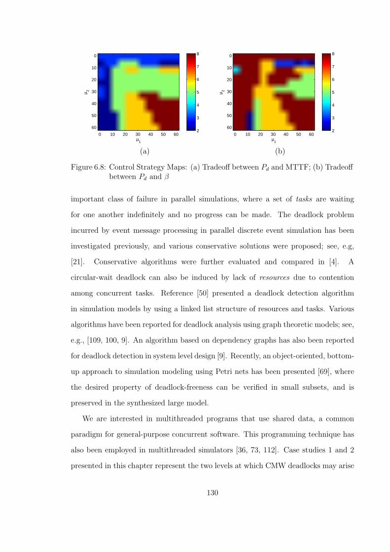
µ1

µ 2

0 10 20 30 40 50 60

0

10

20

30

40

50

602

3

4

5

6

7

8

µ1

µ 2

0 10 20 30 40 50 60

0

10

20

30

40

50

602

3

4

5

6

7

8

(a) (b)

Figure 6.8: Control Strategy Maps: (a) Tradeoff between Pd and MTTF; (b) Tradeoffbetween Pd and β

important class of failure in parallel simulations, where a set of tasks are waiting

for one another indefinitely and no progress can be made. The deadlock problem

incurred by event message processing in parallel discrete event simulation has been

investigated previously, and various conservative solutions were proposed; see, e.g,

[21]. Conservative algorithms were further evaluated and compared in [4]. A

circular-wait deadlock can also be induced by lack of resources due to contention

among concurrent tasks. Reference [50] presented a deadlock detection algorithm

in simulation models by using a linked list structure of resources and tasks. Various

algorithms have been reported for deadlock analysis using graph theoretic models; see,

e.g., [109, 100, 9]. An algorithm based on dependency graphs has also been reported

for deadlock detection in system level design [9]. Recently, an object-oriented, bottom-

up approach to simulation modeling using Petri nets has been presented [69], where

the desired property of deadlock-freeness can be verified in small subsets, and is

preserved in the synthesized large model.

We are interested in multithreaded programs that use shared data, a common

paradigm for general-purpose concurrent software. This programming technique has

also been employed in multithreaded simulators [36, 73, 112]. Case studies 1 and 2

presented in this chapter represent the two levels at which CMW deadlocks may arise

130

in applications: the program source code itself, and the system being simulated in the

case of simulation analysis. Our investigations pertain to deadlocks that may arise

at either of these two levels.

At the program level, the aforementioned tasks are the concurrent threads that

are executing, and the resources are sections of shared data in memory. In this case,

mutexes prevent threads from accessing the same data concurrently, thus allowing

threads to update the shared data in an orderly manner. Misuse of mutexes by

programmers can lead to CMW deadlocks. Case Study 1, presented in Section 6.5.1,

addresses this type of program-level deadlock.

At the system simulation level, the aforementioned tasks and resources can model

various entities in different contexts. For example, in flexible manufacturing system

simulation, the tasks can be parallel assembly lines, and the resources can be machines

processing the parts of a product; in healthcare system simulation, the tasks can be

concurrent patient flows, and the resources can be physicians, nurses, or medical

equipment. In multithreaded simulations, these shared resources are protected via

mutexes by the tasks that first acquire them. If the system design is such that

deadlocks due to shared resources can arise, and no proper efforts are made to avoid

them, then these deadlocks can potentially manifest themselves as CMW deadlocks

when the system is being simulated. Case Study 2, presented in Section 6.5.2,

addresses the deadlock problem at this level.

A similar analytical approach has also been employed to study software contention

in computer systems [91]. Our proposed methodology works for general-purpose

multithreaded software; in particular, it can be applied to multithreaded simulators.

In this latter context, the deadlock-avoidance control logic synthesized by our method

applies to CMW deadlocks at both the aforementioned program and system levels.

In the context of discrete event simulation, in contrast to [69] where Petri nets

have been used in the simulation modeling phase to prevent deadlocks, we focus on

131

existing simulation models and their associated multithreaded programs, which may

be deadlock-prone. Also, in contrast to [109, 100], where graph theoretic models are

used for deadlock detection and resolution, we not only detect deadlocks via formal

methods in Petri nets, but also synthesize optimal control logic to provably prevent

potential CMW deadlocks.

132

CHAPTER VII

Conclusion

7.1 Summary of main contributions

We have adopted a model-based approach and proposed a new class of Petri

nets, called Gadara nets, to systematically model, analyze, and control concurrent

software for the purpose of deadlock avoidance. We have established a set of important

properties of Gadara nets. The liveness and reversibility properties provide a means

to map the behavioral objective of the CMW-deadlock-freeness of a program to the

structural requirement on its corresponding Gadara net model, which in turn lays the

foundations for the structure-based optimal control synthesis of Gadara nets. The

linear separability property further shows the feasibility of optimal control synthesis

through monitor places.

In order to avoid CMW-deadlocks of a program, we require the liveness of its

corresponding Petri net model. Thus, liveness is the key Petri net property under

study in this dissertation. We have proposed a set of customized mathematical

programming algorithms for the verification of liveness of Gadara nets and compared

their performance with generic algorithms that are well-known in the literature. The

proposed algorithms also yield some certain types of siphons that can be used in the

control synthesis.

Based on the established properties of Gadara nets, we have proposed an optimal

133

control synthesis methodology for general Gadara nets that need not be ordinary.

The method is an iterative process and converges in a finite number of iterations.

It exploits the structural properties of Gadara nets via siphon analysis, without the

need to construct the reachability space of the nets. The resulting control logic is

optimal, i.e., it enforces liveness of Gadara nets in a maximally permissive manner.

Our proposed method also takes into account the net uncontrollability and guarantees

that the resulting controlled net is always admissible.

The above general control synthesis methodology possesses an interesting property

that, for any monitor place synthesized by this method, all its incoming and outgoing

arcs have unit arc weights. In the particular application of concurrent software, a

Gadara net model of a program before control is always ordinary, and hence we

always have an ordinary Gadara net as the initial condition in the control synthesis.

This motivates us to investigate the customization of the general control synthesis

methodology for ordinary Gadara nets. The customized methodology preserves all

the properties of the general one, and it has the further property that it will never

synthesize redundant control logic throughout the control iterations.

We have extended the class of untimed Gadara nets to the class of stochastic timed

Gadara nets and proposed a customized discrete event simulation methodology for

the extended class. We have conducted simulation analysis on the Gadara net models

of programs to study a set of performance metrics, including safety, efficiency, and

activity level. We have further conducted sensitivity analysis to investigate the effect

of key parameters on the programs and the implication for deadlock-avoidance control.

The class of Gadara nets together with its associated analysis and control synthesis

techniques provide a novel technology for the systematic, rigorous, principled control

of multithreaded programs. The results developed in this dissertation make it possible

to formalize and automate the procedure of modeling, analyzing, and controlling

multithreaded programs. They also contribute new theoretical developments to the

134

control of Petri nets, which have a significant potential to be extended to a broader

class of resource allocation systems and other application domains [58].

7.2 Future work

For large-scale resource allocation systems, such as concurrent software, scalability

is a key property that must be possessed by the control synthesis algorithms. Our

experiments on large-scale, randomly generated programs demonstrate the attained

efficiency of our methods as compared to some existing approaches. However, our

method did time out on some large, complex sample nets. We observe that the

sole computational bottleneck in the proposed methodology is the MIP algorithms.

Therefore, we are interested in developing even more efficient algorithms for the

detection of unsafe states that correspond to program deadlocks. One potential

direction is to formulate the above detection task as a Boolean satisfiability problem

and leverage the existing SAT solvers to find feasible solutions [12, 29, 46, 66].

We have shown that our proposed methodology will not synthesize redundant

control logic. Yet the number of monitor places synthesized is not minimal in general.

Nazeem et al. [76] exploit the reachability space of the nets and use classification

theory to find a minimum-size control solution in terms of the number of monitor

places. We can further reduce the number of obtained monitor places by using some

of the techniques in this paper.

In practice, a multithreaded program may not satisfy the semiflow condition

(Condition 5 of Definition II.6) for every resource due to programming language

complications and missing information in the CFG representation. For example, a

thread may acquire a lock without releasing it. In this case, users may restore the

semiflow manually, such as adding annotations to the program source code [104]. In

future work, we are interested in automating this process by conducting systematic

lock/unlock pairing analysis [10].

135

An important condition of Gadara nets is that every resource place contains only

one initial token (Condition 6 of Definition II.6), which models the availability of a

mutual exclusion lock. On the one hand, this condition is critical to our development

of the optimal control synthesis algorithms. On the other hand, this condition also

implies that Gadara nets may not be able to model other types of synchronization

primitives, such as semaphore, which is essentially a resource with an arbitrary

capacity. Another example is the reader-writer lock, which allows concurrent readers

and hence requires a resource with a capacity larger than one. Both semaphores and

reader-writer locks can be modeled by resource places with possibly more than one

initial token. Therefore, the modeling of these synchronization primitives calls for an

extension of the existing Gadara net models.

A consequence of relaxing the above condition is that the safe region in the

hyperspace defined by reachable markings may no longer be linearly separable (i.e.,

Theorem III.5 no longer holds for the extended models). As a result, optimal control

logic cannot in general be synthesized through monitor places by SBPI for these

models. Optimal control in this case could be achieved using non-linear policy

structures and representations, such as the generalized algebraic deadlock avoidance

policies proposed previously [90] and the control policies based on classification theory

[74]. We can customize these approaches for the extended Gadara net models.

The Gadara project has opened many new research directions for discrete event

control, where we approach offline synthesis and online implementation in a formal

and integrated framework. From a more general perspective, the results in this

dissertation demonstrate that software failure avoidance is a fertile application area

for discrete event control. Moreover, special features from this application area are

motivating further theoretical developments on the control of discrete event systems.

136

BIBLIOGRAPHY

[1] Allen, L. V. (2010), Verification and anomaly detection for event-based controlof manufacturing systems, Ph.D. thesis, University of Michigan.

[2] Allen, L. V., and D. M. Tilbury (2012), Anomaly detection using modelgeneration for event-based systems without a preexisting formal model, IEEETransactions on Systems, Man and Cybernetics, Part A: Systems and Humans,42 (3), 654–668.

[3] Auer, A., J. Dingel, and K. Rudie (2009), Concurrency control generation fordynamic threads using discrete-event systems, in Proc. Allerton Conference onCommunication, Control and Computing.

[4] Bagrodia, R. L., and M. Takai (2000), Performance evaluation of conservativealgorithms in parallel simulation languages, IEEE Transactions on Parallel andDistributed Systems, 11 (4), 395–411.

[5] Barkaoui, K., and J.-F. Pradat-Peyre (1996), On liveness and controlled siphonsin Petri nets, in Proc. the 17th International Conference on Applications andTheory of Petri Nets, pp. 57–72.

[6] Boer, E. R., and T. Murata (1994), Generating basis siphons and traps ofPetri nets using the sign incidence matrix, IEEE Transactions on Circuits andSystems—I, 41 (4), 266–271.

[7] Cano, E. E., C. A. Rovetto, and J.-M. Colom (2010), An algorithm to computethe minimal siphons in S4PR nets, in Proc. International Workshop on DiscreteEvent Systems, pp. 18–23.

[8] Cassandras, C. G., and S. Lafortune (2008), Introduction to Discrete EventSystems, 2nd ed., Springer, Boston, MA.

[9] Cheung, E., X. Chen, H. Hsieh, A. Davare, A. Sangiovanni-Vincentelli, andY. Watanabe (2009), Runtime deadlock analysis for system level design, DesignAutomation for Embedded Systems, 13 (4), 287–310.

[10] Cho, H. K., Y. Wang, H. Liao, T. Kelly, S. Lafortune, and S. Mahlke (2012),Practical lock/unlock pairing for concurrent programs, Tech. rep., University ofMichigan.

137

[11] Chu, F., and X.-L. Xie (1997), Deadlock analysis of Petri nets using siphons andmathematical programming, IEEE Transactions on Robotics and Automation,13 (6), 793–804.

[12] Claessen, K., N. Een, M. Sheeran, N. Sorensson, A. Voronov, and K. Akesson(2009), SAT-solving in practice, with a tutorial example from supervisorycontrol, Discrete Event Dynamic Systems: Theory and Applications, 19 (4),495–524.

[13] Costa, M., M. Castro, L. Zhou, L. Zhang, and M. Peinado (2007), Bouncer:Securing software by blocking bad input, in Proc. ACM SIGOPS symposiumon Operating systems principles, pp. 117–130.

[14] Delaval, G., H. Marchand, and E. Rutten (2010), Contracts for modular discretecontroller synthesis, in Proc. ACM Conference on Languages, Compilers andTools for Embedded Systems.

[15] Dijkstra, E. W. (1965), Solution of a problem in concurrent programmingcontrol, Communications of the ACM, 8 (9).

[16] Dijkstra, E. W. (1982), Selected Writings on Computing: A PersonalPerspective, chap. The Mathematics Behind the Banker’s Algorithm, pp. 308–312, Springer-Verlag.

[17] Dragert, C., J. Dingel, and K. Rudie (2008), Generation of concurrencycontrol code using discrete-event systems theory, in Proc. ACM InternationalSymposium on Foundations of Software Engineering.

[18] Engler, D., and K. Ashcraft (2003), RacerX: Effective, static detection of raceconditions and deadlocks, in Proc. the 19th ACM Symposium on OperatingSystems Principles.

[19] Ezpeleta, J., J. M. Colom, and J. Martınez (1995), A Petri net based deadlockprevention policy for flexible manufacturing systems, IEEE Transactions onRobotics and Automation, 11 (2), 173–184.

[20] Ezpeleta, J., F. Garcıa-Valles, and J. M. Colom (2002), A banker’s solutionfor deadlock avoidance in FMS with flexible routing and multiresource states,IEEE Transactions on Robotics and Automation, 18 (4), 621–625.

[21] Fujimoto, R. M. (1990), Parallel discrete event simulation, Communications ofthe ACM, 33 (10), 30–53.

[22] Gamatie, A., H. Yu, G. Delaval, and E. Rutten (2009), A case study oncontroller synthesis for data-intensive embedded system, in Proc. InternationalConference on Embedded Software and Systems.

138

[23] Geist, R., J. Hicks, M. Smotherman, and J. Westall (2005), Parallel simulationof Petri nets on desktop PC hardware, in Proc. the 2005 Winter SimulationConference, pp. 374–383.

[24] Gerakios, P., N. Papaspyrou, and K. Sagonas (2011), A type and effect systemfor deadlock avoidance in low-level languages, in Proc. the 7th ACM SIGPLANworkshop on Types in language design and implementation, pp. 15–28.

[25] Gerakios, P., N. Papaspyrou, K. Sagonas, and P. Vekris (2011), Dynamicdeadlock avoidance in systems code using statically inferred effects, in Proc.the 6th Workshop on Programming Languages and Operating Systems.

[26] Ghaffari, A., N. Rezg, and X. Xie (2003), Design of a live and maximallypermissive Petri net controller using the theory of regions, IEEE Transactionson Robotics and Automation, 19 (1), 137–142.

[27] Giua, A. (1992), Petri nets as discrete event models for supervisory control,Ph.D. thesis, Rensselaer Polytechnic Institute.

[28] Giua, A., F. DiCesare, and M. Silva (1992), Generalized mutual exclusionconstraints on nets with uncontrollable transitions, in Proc. 1992 IEEEInternational Conference on Systems, Man, and Cybernetics, pp. 974–979.

[29] Gomes, C. P., H. Kautz, A. Sabharwal, and B. Selman (2008), Handbook ofKnowledge Representation, chap. 2: Satisfiability Solvers, pp. 89–134, Elsevier.

[30] Gurobi (2010), Gurobi Optimizer, http://www.gurobi.com/.

[31] Haas, P. J. (2004), Stochastic Petri nets for modelling and simulation, in Proc.the 2004 Winter Simulation Conference.

[32] Harmon, M. G., T. P. Baker, and D. B. Whalley (1994), A retargetabletechnique for predicting execution time of code segments, Real-Time Systems,7 (2), 159–182.

[33] Heidelberger, P., and D. Nicol (1996), Building parallel simulations from serialsimulators, in Proc. the 4th Annual IEEE/ACM International Symposiumon Modeling, Analysis and Simulation of Computer and TelecommunicationSystems (MASCOTS), pp. 2–4.

[34] Hellerstein, J. L., Y. Diao, S. Parekh, and D. M. Tilbury (2004), FeedbackControl of Computing Systems, Wiley.

[35] Hopcroft, J. E., R. Motwani, and J. D. Ullman (2006), Introduction to AutomataTheory, Languages, and Computation, 3rd ed., Addison Wesley.

[36] Hsu, C.-J., J. L. Pino, and S. S. Bhattacharyya (2008), Multithreadedsimulation for synchronous dataflow graphs, in Proc. the 45th Annual DesignAutomation Conference, pp. 331–336.

139

[37] Iordache, M., and P. Antsaklis (2005), A survey on the supervision of Petrinets, in DES Workshop, Petri Nets 2005.

[38] Iordache, M. V., and P. J. Antsaklis (2006), Supervisory Control of ConcurrentSystems: A Petri Net Structural Approach, Birkhauser, Boston, MA.

[39] Iordache, M. V., and P. J. Antsaklis (2009), Petri nets and programming: Asurvey, in Proc. 2009 American Control Conference, pp. 4994–4999.

[40] Iordache, M. V., and P. J. Antsaklis (2010), Concurrent program synthesisbased on supervisory control, in Proc. 2010 American Control Conference, pp.3378–3383.

[41] Jeng, M., and X. Xie (2001), Modeling and analysis of semiconductormanufacturing systems with degraded behaviors using Petri nets and siphons,IEEE Transactions on Robotics and Automation, 17 (5), 576–588.

[42] Jin, G., L. Song, W. Zhang, S. Lu, and B. Liblit (2011), Automated atomicity-violation fixing, in Proc. the ACM SIGPLAN 2011 Conference on ProgrammingLanguage Design and Implementation.

[43] Joshi, P., C.-S. Park, K. Sen, and M. Naik (2009), A randomized dynamicprogram analysis technique for detecting real deadlocks, in Proc. ACMSIGPLAN conference on Programming language design and implementation,pp. 110–120.

[44] Jula, H., D. Tralamazza, C. Zamfir, and G. Candea (2008), Deadlock immunity:enabling systems to defend against deadlocks, in Proc. the 8th USENIXSymposium on Operating Systems Design and Implementation, pp. 295–308.

[45] Jula, H., S. Andrica, and G. Candea (2012), Efficiency optimizations forimplementations of deadlock immunity, in Runtime Verification, pp. 78–93.

[46] Kautz, H., and B. Selman (2007), The state of SAT, Discrete AppliedMathematics, 155 (12), 1514–1524.

[47] Kavi, K. M., A. Moshtaghi, and D. Chen (2002), Modeling multithreadedapplications using Petri nets, International Journal of Parallel Programming,35 (5), 353–371.

[48] Kelly, T., Y. Wang, S. Lafortune, and S. Mahlke (2009), Eliminatingconcurrency bugs with control engineering, IEEE Computer, 42 (12), 52–60.

[49] Kleijn, J., and M. Koutny (2011), The mutex paradigm of concurrency, in PetriNets 2011, Lecture Notes in Computer Science, pp. 228–247.

[50] Krishnamurthi, M., A. Basavatia, and S. Thallikar (1994), Deadlock detectionand resolution in simulation models, in Proc. the 1994 Winter SimulationConference, pp. 708–715.

140

[51] Kunz, G., O. Landsiedel, S. Gotz, K. Wehrle, J. Gross, and F. Naghibi (2010),Expanding the event horizon in parallelized network simulations, in Proc. the18th Annual IEEE/ACM International Symposium on Modeling, Analysis andSimulation of Computer and Telecommunication Systems (MASCOTS), pp.172–181.

[52] Law, A. M. (2007), Simulation Modeling and Analysis, 4th ed., McGraw-HillCompanies, Inc.

[53] Li, Z., and M. Zhou (2009), Modeling, Analysis, and Deadlock Control ofAutomated Manufacturing Systems, Science Press, Beijing.

[54] Li, Z., and M. Zhou (2009), Deadlock Resolution in Automated ManufacturingSystems: A Novel Petri Net Approach, Springer-Verlag, London.

[55] Li, Z., M. Zhou, and M. Jeng (2008), A maximally permissive deadlockprevention policy for fms based on Petri net siphon control and the theoryof regions, IEEE Transactions on Automation Science and Engineering, 5 (1),182–188.

[56] Li, Z., M. Zhou, and N. Wu (2008), A survey and comparison of Petri net-based deadlock prevention policies for flexible manufacturing systems, IEEETransactions on Systems, Man, and Cybernetics—Part C, 38 (2), 173–188.

[57] Li, Z., N. Wu, and M. Zhou (2010), Deadlock control of automatedmanufacturing systems based on Petri nets - A literature review, Tech. rep.,Xidian University, China.

[58] Liao, H., and M. Lu (2011), A Petri net approach to resource allocation in brandmanagement systems, in Proc. IEEE International Conference on IndustrialEngineering and Engineering Management.

[59] Liao, H., S. Lafortune, S. Reveliotis, Y. Wang, and S. Mahlke (2010), Synthesisof maximally-permissive liveness-enforcing control policies for Gadara Petrinets, in Proc. the 49th IEEE Conference on Decision and Control.

[60] Liao, H., S. Lafortune, S. Reveliotis, Y. Wang, and S. Mahlke (2011), Optimalliveness-enforcing control of a class of Petri nets arising in multithreadedsoftware, conditionally accepted for publication in IEEE Transactions onAutomatic Control.

[61] Liao, H., J. Stanley, Y. Wang, S. Lafortune, S. Reveliotis, and S. Mahlke (2011),Deadlock-avoidance control of multithreaded software: An efficient siphon-based algorithm for Gadara Petri nets, in Proc. the 50th IEEE Conferenceon Decision and Control.

[62] Liao, H., Y. Wang, J. Stanley, S. Lafortune, S. Reveliotis, T. Kelly, andS. Mahlke (2011), Eliminating concurrency bugs in multithreaded software: A

141

new approach based-on discrete-event control, submitted for journal publication,under review.

[63] Liao, H., H. Zhou, and S. Lafortune (2011), Simulation analysis ofmultithreaded programs under deadlock-avoidance control, in Proc. 2011Winter Simulation Conference.

[64] Liao, H., Y. Wang, H. K. Cho, J. Stanley, T. Kelly, S. Lafortune, S. Mahlke, andS. Reveliotis (2012), Concurrency bugs in multithreaded software: Modelingand analysis using Petri nets, Journal of Discrete Event Dynamic Systems.

[65] Liu, C., A. Kondratyev, Y. Watanabe, J. Desel, and A. Sangiovanni-Vincentelli(2006), Schedulability analysis of Petri nets based on structural properties,in Proc. International Conference on Application of Concurrency to SystemDesign.

[66] Marques-Silva, J. P., and K. A. Sakallah (1999), Grasp: a search algorithm forpropositional satisfiability, IEEE Transactions on Computers, 48 (5), 506–521.

[67] Mascarenhas, E., F. Knop, and V. Rego (1995), ParaSol: a multithreadedsystem for parallel simulation based on mobile threads, in Proc. the 1995 WinterSimulation Conference, pp. 690–697.

[68] Moody, J. O., and P. J. Antsaklis (1998), Supervisory Control of Discrete EventSystems Using Petri Nets, Kluwer Academic Publishers, Boston, MA.

[69] Mueller, R., C. Alexopoulos, and L. F. McGinnis (2007), Automatic generationof simulation models for semiconductor manufacturing, in Proc. the 2007 WinterSimulation Conference, pp. 648–657.

[70] Murata, T. (1989), Petri nets: Properties, analysis and applications, Proceedingsof the IEEE, 77 (4), 541–580.

[71] Murata, T., B. Shenker, and S. M. Shatz (1989), Detection of Adastatic deadlocks using Petri net invariants, IEEE Transactions on SoftwareEngineering, 15 (3), 314–326.

[72] Musuvathi, M., S. Qadeer, T. Ball, G. Basler, P. A. Nainar, and I. Neamtiu(2008), Finding and reproducing Heisenbugs in concurrent programs, in Proc.the 8th USENIX Symposium on Operating Systems Design and Implementation.

[73] Mutschler, D. W. (2006), Enhancement of memory pools toward a multi-threaded implementation of the Joint Integrated Mission Model (JIMM), inProc. the 2006 Winter Simulation Conference, pp. 856–862.

[74] Nazeem, A., and S. Reveliotis (to appear), Designing compact and maximallypermissive deadlock avoidance policies for complex resource allocation systemsthrough classification theory: the non-linear case, IEEE Transactions onAutomatic Control.

142

[75] Nazeem, A., S. Reveliotis, Y. Wang, and S. Lafortune (2010), Optimal deadlockavoidance for complex resource allocation systems through classification theory,in Proc. the 10th International Workshop on Discrete Event Systems.

[76] Nazeem, A., S. Reveliotis, Y. Wang, and S. Lafortune (2011), Designingcompact and maximally permissive deadlock avoidance policies for complexresource allocation systems through classification theory: the linear case, IEEETransactions on Automatic Control, 56 (8), 1818–1833.

[77] Nir-Buchbinder, Y., R. Tzoref, and S. Ur (2008), Deadlocks: From exhibitingto healing, in Proc. Workshop on Runtime Verification.

[78] Novark, G., E. D. Berger, and B. G. Zorn (2007), Exterminator: Automaticallycorrecting memory errors with high probability, in Proc. Programming LanguageDesign and Implementation.

[79] Novark, G., E. D. Berger, and B. G. Zorn (2008), Exterminator: Automaticallycorrecting memory errors with high probability, Communications of the ACM,51 (12), 87–95.

[80] Park, J., and S. A. Reveliotis (2001), Deadlock avoidance in sequential resourceallocation systems with multiple resource acquisitions and flexible routings,IEEE Transactions on Automatic Control, 46 (10), 1572–1583.

[81] Park, J., and S. A. Reveliotis (2002), Liveness-enforcing supervision for resourceallocation systems with uncontrollable behavior and forbidden states, IEEETransactions on Robotics and Automation, 18 (2), 234–240.

[82] Park, S., S. Lu, and Y. Zhou (2009), Ctrigger: Exposing atomicity violationbugs from their hiding places, in Proc. 14th International Conference onArchitecture Support for Programming Languages and Operating Systems.

[83] Phoha, V. V., A. U. Nadgar, A. Ray, and S. Phoha (2004), Supervisory controlof software systems, IEEE Transactions on Computers, 53 (9), 1187–1199.

[84] Qin, F., J. Tucek, J. Sundaresan, and Y. Zhou (2005), Rx: Treating bugs asallergies—a safe method to survive software failures, in Proc. the 20th ACMSymposium on Operating Systems Principles, pp. 235–248.

[85] Ramadge, P., and W. M. Wonham (1987), Supervisory control of a class ofdiscrete event processes, SIAM Journal on Control and Optimization, 25 (1),206–230.

[86] Ramadge, P., and W. M. Wonham (1989), The control of discrete event systems,Proceedings of the IEEE, 77 (1), 81–98.

[87] Reisig, W. (1985), Petri Nets: An Introduction, Springer-Verlag.

143

[88] Reveliotis, S. A. (2005), Real-Time Management of Resource AllocationSystems: A Discrete-Event Systems Approach, Springer, New York, NY.

[89] Reveliotis, S. A., and P. M. Ferreira (1996), Deadlock avoidance policiesfor automated manufacturing cells, IEEE Transactions on Robotics andAutomation, 12, 845–857.

[90] Reveliotis, S. A., E. Roszkowska, and J. Y. Choi (2007), Generalized algebraicdeadlock avoidance policies for sequential resource allocation systems, IEEETransactions on Automatic Control, 52 (12), 2345–2350.

[91] Roy, N., A. Dabholkar, N. Hamm, L. Dowdy, and D. Schmidt (2008),Modeling software contention using colored Petri nets, in Proc. the 16th AnnualIEEE/ACM International Symposium on Modeling, Analysis and Simulation ofComputer and Telecommunication Systems (MASCOTS), pp. 1–8.

[92] Shatz, S. M., and W. K. Cheng (1988), A Petri net framework for automatedstatic analysis of Ada tasking behavior, The Journal of Systems and Software,8, 343–359.

[93] Shatz, S. M., S. Tu, T. Murata, and S. Duri (1996), An application of Petrinet reduction for Ada tasking deadlock analysis, IEEE Transactions on Paralleland Distributed Systems, 7 (12), 1307–1322.

[94] Sidiroglou, S., O. Laadan, C. R. Perez, N. Viennot, J. Nieh, and A. D. Keromytis(2009), ASSURE: Automatic software self-healing using rescue points, in Proc.International conference on architectural support for programming languagesand operating systems, pp. 37–48.

[95] Sifakis, J. (1980), Performance evaluation of systems using nets, Net Theoryand Applications, Lecture Notes in Computer Science, 84, 307–319.

[96] Silberschatz, A., P. B. Galvin, and G. Gagne (2008), Operating SystemConcepts, 8th ed., Wiley.

[97] Tricas, F., F. Garcia-Valles, J. Colom, and J. Ezpeleta (2005), A Petri netstructure-based deadlock prevention solution for sequential resource allocationsystems, in Proc. IEEE International Conference on Robotics and Automation,pp. 271 – 277.

[98] URL (Access on April 11, 2012), The Gadara Project, University of Michigan,http://gadara.eecs.umich.edu/.

[99] Uzam, M. (2002), An optimal deadlock prevention policy for flexiblemanufacturing systems using Petri net models with resources and the theory ofregions, International Journal of Advanced Manufacturing Technology, 19 (3),192–208.

144

[100] Venkatesh, S., J. Smith, B. Deuermeyer, and G. Curry (1998), Deadlockdetection and resolution for discrete-event simulation: multiple-unit seizes, IIETransactions, 30 (3), 201–216.

[101] Wallace, C., P. Jensen, and N. Soparkar (1996), Supervisory control of workflowscheduling, in Proc. International Workshop on Advanced Transaction Modelsand Architectures.

[102] Wang, J. (1998), Timed Petri Nets: Theory and Application, Kluwer AcademicPublishers.

[103] Wang, Y. (2009), Software failure avoidance using discrete control theory, Ph.D.thesis, University of Michigan.

[104] Wang, Y., T. Kelly, M. Kudlur, S. Lafortune, and S. A. Mahlke (2008), Gadara:Dynamic deadlock avoidance for multithreaded programs, in Proc. the 8thUSENIX Symposium on Operating Systems Design and Implementation, pp.281–294.

[105] Wang, Y., S. Lafortune, T. Kelly, M. Kudlur, and S. Mahlke (2009), Thetheory of deadlock avoidance via discrete control, in Proc. the 36th Annual ACMSIGPLAN-SIGACT Symposium on Principles of Programming Languages, pp.252–263.

[106] Wang, Y., H. Liao, A. Nazeem, S. Reveliotis, T. Kelly, S. Mahlke,and S. Lafortune (2009), Maximally permissive deadlock avoidance formultithreaded computer programs (extended abstract), in Proc. the 5th AnnualIEEE Conference on Automation Science and Engineering, pp. 37–41.

[107] Wang, Y., H. Liao, S. Reveliotis, T. Kelly, S. Mahlke, and S. Lafortune (2009),Gadara nets: Modeling and analyzing lock allocation for deadlock avoidancein multithreaded software, in Proc. the 48th IEEE Conference on Decision andControl, pp. 4971–4976.

[108] Wang, Y., H. K. Cho, H. Liao, A. Nazeem, T. P. Kelly, S. Lafortune, S. Mahlke,and S. Reveliotis (2010), Supervisory control of software execution for failureavoidance: Experience from the Gadara project, in Proc. InternationalWorkshop on Discrete Event Systems.

[109] Woodward, E. E., and G. T. Mackulak (1997), Detecting logic errors in discrete-event simulation: reverse engineering through event graphs, Simulation Practiceand Theory, 5 (4), 357–376.

[110] Yamalidou, K., J. Moody, M. Lemmon, and P. Antsaklis (1996), Feedbackcontrol of Petri nets based on place invariants, Automatica, 32 (1), 15–28.

[111] Zeng, F. (2009), Pattern-driven deadlock avoidance, in Proc. the 7th Workshopon Parallel and Distributed Systems: Testing, Analysis, and Debugging.

145

[112] Zuberek, W. M. (2009), Performance limitations of block-multithreadeddistributed-memory systems, in Proc. the 2009 Winter Simulation Conference,pp. 899–907.

146